Development and Demonstration of a TDOA-BasedGNSS Interference Signal Localization System

Jahshan A. Bhatti, Todd E. Humphreys, The University of Texas at Austin, Austin, TXBrent M. Ledvina, Coherent Navigation, San Mateo, CA

Abstract—Background theory, a reference design, and demon-stration results are given for a Global Navigation SatelliteSystem (GNSS) interference localization system comprising adistributed radio-frequency sensor network that simultaneouslylocates multiple interference sources by measuring their signals’time difference of arrival (TDOA) between pairs of nodes inthe network. The end-to-end solution offered here draws fromprevious work in single-emitter group delay estimation, very longbaseline interferometry, subspace-based estimation, radar, andpassive geolocation. Synchronization and automatic localizationof sensor nodes is achieved through a tightly-coupled receiverarchitecture that enables phase-coherent and synchronous sam-pling of the interference signals and so-called reference signalswhich carry timing and positioning information. Signal and cross-correlation models are developed and implemented in a simulator.Multiple-emitter subspace-based TDOA estimation techniquesare developed as well as emitter identification and localizationalgorithms. Simulator performance is compared to the Cramér-Rao lower bound for single-emitter TDOA precision. Results aregiven for a test exercise in which the system accurately locatesemitters broadcasting in the amateur radio band in Austin, TX.

I. INTRODUCTION

Despite its marvelous success over the last three decades,the Global Positioning System (GPS) has an Achilles’ heel:its weak signals are an easy target for jamming. The NationalSpace-Based Positioning, Navigation, and Timing AdvisoryBoard in a recent white paper has concluded that the “UnitedStates is now critically dependent on GPS” [1]. The papernotes an alarming increase in the incidence rate of deliberateand unintentional GPS interference, which in some casesrenders GPS inoperable for critical infrastructure operations.The white paper also notes the increasing availability of smalland cheap GPS jammers known as personal privacy devices(PPDs). Although the advertised jamming coverage radius forthese devices is small, typically 10 to 20 meters, their actualrange may extend to tens of kilometers [2].

In one recent case of interest, a test version of the GPSground-based augmentation system (GBAS) at Newark Inter-national Airport suffered from periodic interference due toa PPD aboard a truck traveling on a nearby highway [3].The authorities took four months to track down the jammer.Continued monitoring in the Newark airport area after thisincident indicates that during rush hours, there occur 4 to5 interference events per hour, presumably due to PPDs [4].GPS-synchronized cellular communications networks also re-port an increasing rate of periodic GPS outages, most likelydue to passing PPDs. Although these networks are designedto fall back to a hold-over mode that is capable of maintaining

adequate synchronization for several days, such interference isnonetheless an annoyance for network operators.

Despite a recent effort by the Federal CommunicationsCommission to discourage sale, purchase, and use of PPDs [5],there is reason to believe that they will only become morewidespread in the future. The miniaturization and proliferationof GPS trackers will likely lead to an increased use of PPDs,despite their being illegal, as people seek to protect theirprivacy from invasive tracking [6]. To aid in enforcing lawsagainst PPDs and jamming devices, there is a need for apersistent system capable of detecting and locating sourcesof jamming.

There is extensive literature on passive geolocation andtime difference of arrival (TDOA) estimation. This paperdevelops an interference localization solution that is basedon maximum likelihood TDOA estimation techniques whichcan be traced back to the 1970s [7–9]. These techniquesare based on analysis of the cross-power spectral density(CPSD) of an emitter signal received at two sensors withsome differential delay. The very long baseline interferometry(VLBI) community uses similar techniques to estimate thegroup delay between the received signals at separate referencestations [10].

For single-emitter TDOA estimation, it is often sufficientto choose the delay that maximizes the time-domain cross-correlation function [11–14]. However, for multiple emitters,analysis of the CPSD offers better resolution because pow-erful subspace methods such as multiple signal classification(MUSIC) can be applied to distinguish the frequency-domaincomponents due to the various emitters [15].

In so-called passive geolocation, where the structure ofthe interference signals is not known a priori, the estimatedTDOAs must be associated with emitters. In other words, onemust decide from which emitter, if any, a TDOA measure-ment originated. Previous solutions to the data associationproblem, which require solving a computationally-demandinghigh-dimensional assignment problem, are reviewed in [16],and a computationally-efficient “tracking” extension of theproblem is introduced. The effect of non-line-of-sight TDOAmeasurements due to multipath reflections and ways to detectthose measurements through consistency checks are consid-ered in [14].

More particularly related to the problem of locating GPSinterference sources, the work by Scott (J911) [17], Brown(JLOC) [18], and Chronos Technology (GAARDIAN) [19]focus on building cheap, low-network-throughput jamming-to-

Copyright c© 2012 by Jahshan A. Bhatti,Todd E. Humphreys, Brent M. Ledvina

1 Preprint of the 2012 IEEE/ION PLANS ConferenceMyrtle Beach, SC, April 21–23, 2012

noise ratio sensors based on monitoring GPS carrier-to-noiseratio and automatic gain control (AGC) values, making themsuited only for triggering and coarse localization. The workby Akos considers a network of sensor nodes using a low-cost Global Navigation Satellite System (GNSS) front endwith AGC monitoring capability. Single-emitter interferencelocalization is implemented using AGC values coupled withpower-law path loss models for strong sources and cross-correlation-based TDOA estimation coupled with hyperbolicpositioning for weak sources [11, 12].

The current paper offers a thorough overview of the emitterlocalization problem and describes the design and implementa-tion of an operational prototype system targeted to GNSS inter-ference source detection and localization. Theoretical modelsfor received signals from multiple emitters are developedwith appropriate assumptions for typical terrestrial emitterlocalization applications. For improved location precision, theprototype system is implemented with a spatially-distributedarray of sensor nodes. The technique of synchronizing sensornodes by clock-sharing via coaxial cable, as in [13], cannotbe applied to this system because the sensors are separated bykm-length baselines. Instead, the sensors make use of ambientradio frequency (RF) timing signals such as GPS or cellularcode division multiple access (CDMA) to provide timingsynchronization [11, 20]. For sensors on moving platforms, aposition, velocity, and time solution (commonly obtained fromGNSS signals) is required to synchronize the correlator’s timeand frequency offset.

The current work extends the previous work on TDOA-based GNSS interference source localization in [11, 13] byemphasizing simultaneous localization of multiple emitters.The multiple-emitter problem is addressed under reasonableassumptions about the emitter signal spectral shape, allowingthe TDOAs to be detected and estimated in a straightforwardsubspace and least-squares fitting framework. The problemof TDOA data association is addressed through a simple buteffective phase closure consistency check which assumes thatthe TDOA measurements are not significantly affected bymultipath. A simulator developed to provide a testbed forvalidating theory and refining algorithms is described and bothsimulated and field-test results for the localization algorithmsare provided.

II. SIGNAL MODELS

The models developed in this section form the basis of theTDOA estimation algorithms. The development is guided byderivations given in the radar literature [21], but adapted forpassive geolocation.

A. Received Signal Model

Consider the following model for the signal transmitted byan interference source (hereafter emitter):

s (t) = As (t) cos (2πfct+ φs (t)) . (1)

Here, As (t) is the instantaneous amplitude, fc is the cen-ter frequency, and φs (t) is the transmitted beat carrier

phase. For convenience, consider the complex envelopes (t) = As (t) exp (jφs (t)) and analytic representation s (t) =s (t) exp (2πfct) of the transmitted signal s (t). Note thatanalytic signals are a valid approximation when the complexenvelope is slowly varying with respect to the center frequency(i.e. bandpass signals) [21]. Assume that the radio propagationchannel induces a non-dispersive delay τρ (t), an attenuationA (ρ) that is a function of the average range ρ over the time-of-flight interval, and additive white Gaussian noise n′ (t). Thenthe received signal r′ (t) at the sensor can be modeled as

r′ (t) = A (ρ) s (t− τρ (t)) + n′ (t) , (2)

or with an analytic representation as

r′ (t) = A (ρ) s (t− τρ (t)) + n′ (t) , (3)

where n′ (t), the analytic representation of n′ (t), is a complexwhite Gaussian noise process with single-sided power spectraldensity N0 in W/Hz. Other propagation effects like multipathand shadowing are not considered in this model.

For electromagnetic waves traveling in a vacuum, the prop-agation delay τρ (t) satisfies the implicit relationship

cτρ (t) =

√(re (t− τρ)− rs (t))

T(re (t− τρ)− rs (t)),

(4)where c is the speed of light, rs (t) is the sensor positionvector, and re (t) is the emitter position vector [22]. For shortpropagation distances and electromagnetic wave velocities, (4)can be approximated as

cτρ (t) = ρ (t) =

√r (t)

Tr (t), (5)

where r (t) = re (t) − rs (t) is the relative position vectorand ρ (t) is the instantaneous range. The range rate is givenby ρ (t) = r (t)

Tr (t) /ρ (t). In a further approximation

that applies to emitters and sensors with moderate standoffdistances and terrestrial velocities, the delay can be modeledlinearly as

cτρ (t) = ρ (0) + ρ (0) t (6)

over a small interval of time about t = 0.Let the relationship between the time tr at the sensor and

true time t be given by

t = tr − τr (tr) , (7)

where τr (tr) is the sensor’s clock offset from true time. Theclock is parametrized by a sensor clock offset bias af0 andclock offset drift or fractional frequency error af1 so that thesensor’s clock offset time history τr (tr) is given by

τr (tr) = af0 + af1tr. (8)

The linear model is valid for the clocks used in this applicationover a small interval of time about tr = 0 where small isdefined as less than 100 ms for a temperature-compensatedcrystal oscillator or 10 s for an oven-controlled crystal oscil-lator.

2

Suppose that a mixing signal with nominal center frequencyfc is generated with the sensor’s clock. The mixing signal’sphase φr (tr) is related to tr by

φr (tr) = 2πfctr + φr,0, (9)

where φr,0 is the initial phase of the oscillator. Let the mixingoperation be modeled such that the resulting baseband signalr′ (t) is given by

r′ (t) = r′ (t) exp (−jφr (tr))

= A (ρ) s (t− τρ (t)) exp (−jφ′ (t, tr)) + n′ (t) , (10)

where

φ′ (t, tr) = 2π (tr − t+ τρ (t)) fc + φr,0 (11)

and n′ (t) = n′ (t) exp (−jφr (tr)) is a zero-mean basebandcomplex Gaussian process. The sensor clock model in (7) isused in (10) to express r′ (t) in the sensor’s time base, denotedr (tr). The noise-free baseband received signal sr (tr) is givenby

sr (tr) = A (ρ) s (tr − τm (tr)) exp (−jφm (tr)) , (12)

with the apparent delay τm (tr) defined as

τm (tr) = τr (tr) + τρ (tr − τr (tr)) (13)

and the received beat carrier phase φm (tr) given by

φm (tr) = 2πfcτm (tr) + φr,0. (14)

The full expression for the baseband received signal r (tr) isgiven by

r (tr) = sr (tr) + n (tr) , (15)

where n (tr) = n′ (tr − τr (tr)) is still a zero-mean basebandcomplex Gaussian process. Given the aforementioned linearapproximations for the clock and range delays, the apparentdelay can be approximated by linear parameters τm,0 and τmas

τm (tr) ≈ τm,0 + τmtr. (16)

Assuming a nominal sampling rate Ts, the digital represen-tation of the signal r (tr) is given by r[k] = r (kTs). The noisen (tr) is generated at each sensor based on the noise powerdensity N0 in W/Hz over the single-sided noise-equivalentbandwidth Bn in Hz. Therefore, the noise power σ2

n in Wattsis given by

σ2n = N0Bn. (17)

The complex noise time series n[k] is a scaled and filteredversion of a sequence of random samples whose real and imag-inary components are independent and normally distributed.The noise samples are scaled so that

E [n[k]n?[k]] = 2σ2n. (18)

The emitter has an average transmitted power density Ps inW/Hz over the single-sided noise-equivalent bandwidth. Thespreading loss L (ρ) is given by

L (ρ) =λ2c

4π2ρ2, (19)

where λc = c/fc is the nominal wavelength of the signal.Isotropic transmit and receive antennas and no cable loss areassumed. The received signal power σ2

s in Watts is given by

σ2s = L (ρ)PsBn. (20)

The signal component of the received signal sr[k] = sr (kTs)is scaled so that

E [sr[k]s?r [k]] = 2σ2s , (21)

which constrains A (ρ) in (2) appropriately.Finally, the received signal ri (tr) at sensor i from M

emitters can be modeled as a sum of components of the formin (15):

ri (tr) =

M∑l=1

A(ρli)sl(tr − τ lmi

(tr))

(22)

× exp(−j[2πfcτ

lmi

(tr) + φri,0])

+ ni (tr) ,

where the apparent delay for emitter l and sensor i is definedas a specialization of (13):

τ lmi(tr) = τri (tr) + τ lρi (tr − τri (tr)) . (23)

B. The Cross-Ambiguity Function

Consider the following narrowband cross-ambiguity func-tion Szizk (τ, fD), which has been adapted from the radarliterature [21], for a pair of complex baseband signals zi (t)and zk (t):

Szizk (τ, fD) ,1

T

ˆ T/2

−T/2zi (t) z?k (t+ τ) e−j2πfDtdt, (24)

where T is the length of the integration interval, τ is thedelay, and fD is the Doppler frequency. The forthcomingequations will be simplified by using the difference operator∆ik (·) = (·)k − (·)i, that is, the placement of a ∆ik in frontof a quantity indicates a difference of that quantity betweensensors i and k. The cross-ambiguity function Srirk (τ, fD)for a pair of signals ri (t) and rk (t) from receivers i andk, respectively, using the single-emitter propagation modelin (15) and linearized apparent delay is approximately givenby

Srirk (τ, fD) ≈ αikSss (τ −∆ikτm,0, fD −∆ik τmfc)

+Nik (τ, fD) , (25)

where the complex attenuation factor αik is defined as

αik = A (ρi)A (ρk) ej[2π∆ikτm,0fc+∆ikφr,0] (26)

and Nik (τ, fD) is the noise function, which includes allcorrelation terms involving the noise signal n (t). In (25),it is assumed that the apparent range rate τm, which is

3

related to the velocity of the emitter and oscillator clock driftrate, is small and has negligible impact on the correlationover the integration interval. The impact is negligible if thebandwidth of the baseband signal s (t) is small with respectto the carrier frequency fc. This is known as the narrowbandapproximation [21]. The delay and Doppler that maximizethe magnitude of the ambiguity function, denoted respectivelyas τik and fD,ik, are the corresponding time and frequencydifference of arrival (T/FDOA) measurements between sensorsi and k for a single emitter [21].

Again, invoking the narrowband approximation, the cross-ambiguity function Srirk (τ, fD) can be written for M emittersin terms of the auto-ambiguity terms Aik (τ, fD), the cross-ambiguity terms Cik (τ, fD), and the noise terms Nik (τ, fD),as

Srirk (τ, fD) ≈ Aik (τ, fD)+Cik (τ, fD)+Nik (τ, fD) . (27)

The auto-ambiguity terms are of most interest and can bewritten as

Aik (τ, fD) =

M∑l=1

αlikSslsl(τ −∆ikτ

lm,0, fD −∆ik τ

lmfc

),

(28)where the complex attenuation factor αlik is defined as

αlik = A(ρli)A(ρlk)ej[2π∆ikτ

lm,0fc+∆ikφr,0]. (29)

The cross-ambiguity terms are generally small in the delay-Doppler range of interest provided that there is no strictcoordination between emitters.

III. SYNCHRONIZATION AND SIGNAL EXCISION

A. Tightly-Coupled Sensor Architecture

“Tightly-coupled” refers to an RF receiver architecturein which emitter signals and reference signals are down-converted with the same oscillator and sampled in such away that a nanosecond-accurate correspondence can be madebetween the two sampled signal streams (coherent signalconditioning and sampling). Fig. 1 shows one straightforwardtightly-coupled sensor architecture. Tight coupling betweenthe emitter and reference data enables the data streams fromtwo separate sensors to be synchronized to within nanosecondsand for clock variations over the cross-correlation interval tobe estimated and compensated at the carrier-phase level. Thetightly-coupled sensor architecture draws from the success ofongoing work in opportunistic navigation at the University ofTexas at Austin [20, 23, 24]. Experience with GNSS signals,terrestrial signals of opportunity such as cellular CDMA, andIridium signals suggests that an emitter localization systemcould exploit any instance of these three signal types as areference.

The simplest approach to a tightly-coupled sensor archi-tecture is to use GNSS signals as the reference signals. Thisapproach allows one to exploit the well-known, clean, andstable signal characteristics of GNSS signals. GNSS signalprocessing can be done within the sensor to minimize networkthroughput requirements. For example, consider using GNSS

Signals

Signals Reference

Single Driving Clock

Signal

Conditioning

Reference Signals

Joint Processing

of Emitter and

Emitter

A/D

Figure 1: Basic tightly-coupled sensor architecture.

timing to synchronize stationary sensors in known locations.A typical GNSS navigation solution will provide estimatesof the receiver clock offset τr,0 and offset rate τr. For somesufficiently small time window, a linear model can be appliedto the clock offset τr (tr) = τr,0 + τrtr. Then, (7) can besolved for receiver time in terms of true time as

tr (t) =t+ τr,01− τr

= α+ (1 + β) t, (30)

where α =τr,0

1−τr and β = τr1−τr . Invoking the narrowband

signal assumption, the baseband synchronized signal rs (t) isgiven by

rs (t) ≈ r (t+ α) exp (j2πβfct) . (31)

Therefore, for small clock offset rates, the operations requiredfor synchronization are simply a delay and complex mixingoperation.

One might naturally question the wisdom of using GNSSsignals as reference signals by pointing out that the emitterto be located may be broadcasting a strong interfering signalwithin GNSS frequency bands. In this case, the received GNSScarrier-to-noise ratios might be too low to support makingreliable timing estimates. This paper addresses this concernin several ways.

First, significant frequency diversity is offered by the com-bined spectrum assets of modern GNSS systems like GPS,Galileo, GLONASS, and Compass. If any one of the manysignal bands within these separate systems is free of interfer-ence, then signals from this band can be taken as referencesignals. An in-house software-defined radionavigation process-ing engine, named “GRID,” can be embedded for execution onthe sensors themselves and is currently capable of acquiringand tracking GPS L1 C/A and GPS L2C signals [20, 25–28].With some fairly straightforward extensions, the GRID engineis capable of acquiring and tracking all CDMA-based GNSSsignals, including GPS L5, GPS L1C, Galileo, Compass, andfuture CDMA versions of GLONASS signals.

Another approach to mitigating the effects of interferenceon reference signals drawn from GNSS bands is to draw thereference signals in via a directional antenna. For stationarysensors, a single GNSS signal is all that is required to providethe benefits of a tightly-coupled sensor architecture. Hence,if each sensor is equipped with a directional antenna that

4

can recover sufficient signal power from just one GNSSsatellite (not necessarily the same satellite at each sensor),then the requisite synchronization between the two sensors’data streams can be established. For example, an inexpensivehelical antenna pointed toward zenith would have a goodchance of capturing the requisite GNSS signal and suppressinga surface-based interference signal.

A third option for dealing with the in-GNSS-bands inter-ference scenario is to capture non-GNSS signals that could beexploited in the same way as GNSS signals to synchronize andstabilize the recorded emitter data. Research at the Universityof Texas at Austin has shown that forward-link CDMA cellularpilot signals are an excellent reference for tightly-coupledreceivers [20, 23, 24]. Typical CDMA cellular base stationstransmit signals that arrive with 40 dB greater power thanGPS signals, are synchronized to GPS time to within a fewmicroseconds, and offer coherence times at L-band in excessof 100 s [20]. Periodic calibration of forward-link signalsduring times of GNSS availability can reduce CDMA signals’timing uncertainty to nanoseconds. Thus, for applicationswhere CDMA cellular signals are available—for example,within the US—they represent an excellent backup to GNSSsignals for tightly-coupled emitter localization. The GRIDsoftware-defined radionavigation processing engine is capableof acquiring and tracking forward-link CDMA cellular pilotsignals (see Fig. 2). As with GNSS signals, this processingcan be executed onboard the sensors.

============ GRID: General Radionavigation Interfusion Device =============Receiver time: 0 weeks 160.0 seconds Build ID: 1379GPS time: 1614 weeks 420784.0 seconds

---------------------------------------------------------------------------CH TXID Doppler BCP PR C/N0 Az El Status

(Hz) (cycles) (meters) (dB-Hz) (deg) (deg)-------------------------GPS_L1_CA Channels--------------------------------1 1u 430.75 -76149.17 20972555.14 46.3 301.7 12.9 62 2 -2337.63 372213.50 20793027.57 44.1 93.0 10.8 63 5 -2814.11 449035.30 19188750.37 52.3 42.0 32.0 64 15 2229.20 -362763.30 17919804.83 53.6 149.9 48.9 65 18 2228.97 -360186.88 19526452.99 48.6 243.3 29.8 66 21 2027.74 -324302.89 19403848.18 51.0 306.8 34.8 67 25 -2734.77 436530.00 20267387.49 47.7 218.6 19.7 68 26 410.60 -75412.16 17644648.06 54.0 88.4 47.0 69 29 398.14 -71226.59 16810240.92 52.1 287.2 79.5 6

10 30 -731.36 110014.30 20121635.88 46.5 282.3 18.5 611 -- --------- ------------ ----------- ---- ------ ----- -12 -- --------- ------------ ----------- ---- ------ ----- --------------------------CDMA_UHF_PILOT Channels---------------------------1 1 -0.59 91.58 7622658.88 62.0 0.0 0.0 5

------------------------------Navigation Data------------------------------X: -745467.86 Y: -5462657.31 Z: 3196401.16 deltRx: -3464962.30Xvel: 0.03 Yvel: -0.04 Zvel: 0.01 deltRxDot: 0.12

===========================================================================

Figure 2: Screen output of the GRID software-defined radion-avigation engine showing simultaneous tracking of 10 GPS L1C/A signals and 1 CDMA cellular forward-link pilot signal.

B. Reference Signal Excision

If the emitter and reference signal band are the same,then the ambient reference signals will cross-correlate inthe same way as the emitter signals. Therefore, to improvesensitivity to the emitters of interest, it is advantageous totrack and remove the ambient reference signals if they havehigh enough carrier-to-noise ratios before cross-correlation. InCDMA systems, the loss of sensitivity to weak emitters in thepresence of strong emitters is known as the near-far effect,and interference cancellation is a commonly-used technique

to solve this problem [29, 30]. In addition, the technique wasused in [31] to crack the Galileo test codes using the L1-band signals received from a patch antenna, where a softwareGPS receiver was used to acquire, track, and remove thenuisance GPS/SBAS signals. Ref. [12] considers the sameissue when trying to locate weak emitters in the GPS bandand solves the problem by using a notch filter to removethe ambient GPS signals before cross-correlation. However,the notch filtering technique is suboptimal and reduces theavailable emitter signal power that could be used in cross-correlation.

IV. TDOA ESTIMATION

Many parallels can be drawn between VLBI, active radar,and passive geolocation. In the 1970s, high resolution timedelay estimation techniques were developed [7, 8] using delay-parameterized models of the phase of the cross-power spec-trum (e.g. a linear model for non-dispersive delays). Similarly,in the VLBI community, the group delay estimate is typicallycouched in terms of a least-squares fit to the slope of the phaseof the cross-power spectrum (see Appendix 12.1 of [10]). Ithas been shown in [32] that this least-squares approach isequivalent to the maximum likelihood estimator developedin [7, 8].

Traditional radar techniques use matched filtering (MF) todetermine the delay and Doppler of targets, which is analogousto examining the cross-ambiguity function in passive geoloca-tion as in [12–14]. However, MF is limited by the support ofthe ambiguity function of the transmitted waveform. As a re-sult, its delay resolution tends to be on the order of the inverseof the bandwidth of the transmitted waveform, and its Dopplerresolution tends to be on the order of the temporal supportof the transmitted waveform [21, 33]. Therefore, the abilityof MF-based methods to distinguish between two closely-spaced targets is severely limited in the delay-Doppler space.In addition, the output of the matched filter leads to peaksthat are not centered at the true targets for a majority of thetargets due to the superposition of interfering ambiguity func-tions. Ref. [33] provides a framework for “super-resolution”radar that bypasses the aforementioned limitations for MF byparametrization of the response with a finite set of delaysand Doppler-shifts and application of parametric estimationtechniques like subspace methods. Non-parametric estimationtechniques discretize the delay and Doppler space into agrid and determine if a target is present at each grid point.Given the limitations of non-parametric estimation especiallyunder multiple targets, a parametric approach to estimating theTDOA of emitters is developed in the subsequent subsection.

A. A Parametric Approach to TDOA Estimation

Consider the following model for the CPSD between a pairof sensors,

Yrirk (f) =

M∑l=1

αlikYslsl (f) e−j2πfτlik +Nrirk(f), (32)

5

where αlik and τ lik are respectively the complex scale factorand the TDOA between sensors i and k of emitter l, Yslsl (f)is the normalized power spectral density of emitter l, andNrirk(f) contains terms due to noise and cross-correlationbetween the emitter waveforms. Note that the CPSD couldbe estimated by the discrete Fourier transform of a Dopplercut at some fD of an estimate of the ambiguity functionRrirk (τ) = Srirk (τ, fD). Note that in the case of synchro-nized sensors and stationary emitters and sensors, fD = 0.The ambiguity function should be windowed appropriately sothat only delays of interest, which are driven by the sensorpair’s baseline or known emitter waveform repetition rate,are considered. Assuming that the emitter waveforms havenormalized, wide, flat frequency spectra (Yslsl (f) = 1) andare uncorrelated (E [Nrirk(f)] = 0), then the measurementmodel for the power spectral density is given by

Yrirk (f) =

M∑l=1

αlik exp(−j2πfτ lik

)+Nrirk (f) . (33)

The problem is now in terms of parametric estimation of com-plex exponentials in noise, a well-studied problem [15, 34].First, guesses for the TDOAs and the number of emitters areinitialized using subspace methods like MUSIC [15]. Then,estimates of the power and TDOAs are iterated in a least-squares fitting algorithm until a convergence condition is met.The complex scale factors are estimated using linear leastsquares fitting (note that αlik appears linearly in Yrirk (f))and the TDOAs are updated using an iteration of nonlinearleast squares fitting.

B. Subspace Methods for TDOA Estimation

A brief description of subspace methods is provided. Con-sider a tapped delay line of length K > M that uniformlysamples Yrirk (f) with sampling interval ∆f . The data modelfor the tapped delay line is given in (34) on the next page,where fk = f0 + k∆f , or, in vector form,

Y = EA + N, (35)

where A ∈ CM×1 is a vector of complex scale factors,E ∈ CK×M is a matrix composed of mode vectors e (τ) ∈CK×1, and N ∈ CK×1 is a complex noise vector, withreal and imaginary parts distributed normally N

(0, σ2

nI)

anduncorrelated with the parameters. The mode vector e (τ) isgiven by

e (τ) =

exp (−j2πf1τ)exp (−j2πf2τ)

...exp (−j2πfKτ)

. (36)

Let the K ×K covariance matrix S be defined as

S = E[YYH

]= EE

[AAH

]EH + σ2

nE[NNH

]= EPEH + σ2

nI, (37)

where P is the covariance of the complex scale factors. Givena single, uniformly sampled observation of Yrirk (f) of lengthP with sampling interval ∆f , x[k], the covariance matrixcan be estimated using the “forward-backward” averagingmethod [35] as

S = XHX, (38)

where

X =

x[K + 1] · · · x[1]...

. . ....

x[P −K] · · · x[K + 1]...

. . ....

x[P ] · · · x[P −K]x?[1] · · · x?[K + 1]... . .

. ...x?[K + 1] · · · x?[P −K]

... . .. ...

x?[P −K] · · · x?[P ]

. (39)

The K eigenvectors vi and eigenvalues λi of S must satisfySvi = λivi, for i = 1, 2, . . . ,K. Assuming that all the modevectors are linearly independent (i.e. E has full rank), then forM < K, the matrix EPEH is singular and it can be shownthat S has K−M eigenvalues equal to σ2

n. In fact, an estimateof M can be computed by subtracting the multiplicity of σ2

n inthe eigenvalues of S from K. Since S = EPEH + σ2

nI, thenEPEHvi =

(λi − σ2

n

)vi is true. Note that for each eigenvalue

λi = σ2n, EHvi = 0, i.e. the “signal” subspace E (spanned by

the mode vectors) is orthogonal to the “noise” subspace EN(spanned by the eigenvectors associated with λi = σ2

n) [15].Note that in practice, only estimates of S are available,

and the aforementioned conditions are only approximatelysatisfied. Therefore, the eigenvalues associated with the noisesubspace are not exactly σ2

n, and instead are clustered aboutσ2n (and the spread of the cluster decreases with more averag-

ing) [15]. Estimating M can be particularly difficult when thegap between the eigenvalues associated with the signal andnoise subspace is not clear. Hypothesis tests for estimatingM were developed using matrix perturbation theory in [35].However, for ease of implementation and prototyping, thepresent algorithms require a priori knowledge of M and/orsubjective analysis of the eigenvalues of S (or equivalentlythe singular values of X). The MUSIC cost function is givenby

JMU (τ) = eH (τ)ENEHNe (τ) , (40)

which for uniformly sampled signals, can be minimized usingRoot-Music [36, 37].

The above algorithms are limited in that the data modelassumes flat emitter frequency spectra. The performance ofthe algorithms degrade with model mismatch, and in par-ticular, simulation results indicate MUSIC makes biased orspurious TDOA estimates when the flat spectra assumption isrelaxed. Also, the resolvability of two closely-spaced TDOAsdecreases as their separation decreases in the presence of noise.

6

Yrirk (f1)Yrirk (f2)

...Yrirk (fK)

=[e(τ1ik

)e(τ2ik

)· · · e

(τMik)]α1ik

α2ik...αMik

+

Nrirk (f1)Nrirk (f2)

...Nrirk (fK)

(34)

The mode vectors associated with closely-spaced TDOAs arenearly linearly dependent, which causes the one of the eigen-vectors in the signal subspace to have a small eigenvalue. Inthe presence of noise, the eigenvector can not be distinguishedfrom the noise subspace if the associated eigenvalue is toosmall, hence the loss of resolution.

V. EMITTER IDENTIFICATION AND LOCALIZATION

In passive geolocation, the estimated TDOAs between allpossible pairs of sensors must be associated with possibleemitters. Sathyan and others have proposed algorithms to solvethis data association problem inherent in passive geoloca-tion [16]. However, the currently implemented algorithm usesthe principle of phase closure to verify that a triad of TDOAmeasurements can be associated with the same emitter. Theclosure-based algorithm is a simple and effective prototype butmore sophisticated methods may be implemented if they proveto be more effective. Consider three true (noise-free) times ofarrival (TOAs) of an emitter signal τi, τj , and τk to sensorsi, j, and k, respectively. The sensors can be paired in threeways, forming three true TDOAs: τij = τj−τi, τik = τk−τi,and τjk = τk − τj . The TDOA measurements

τij = τij + nij (41)

are assumed to be corrupted by zero-mean noise nij withcovariance given in [13, p. 64]. The TDOA closure metricis defined as

τc = τij − τik + τjk. (42)

Under the hypothesis that the TDOA measurements are as-sociated with an emitter, then E [τc] = 0 and E

[τ2c

]=

E[(nij − nik + njk)

2]. A test can be constructed in which

a threshold τc,th is chosen such that τ2c < τ2

c,th indicatesthat the TDOA measurements under test can be associatedwith the same emitter for a certain probability of false alarm,although this paper does not carry out the entire analysis ofthe detection statistic. If a triplet of TDOA measurements“close,” then, geometrically, the three hyperbolas intersect ata single point on a plane. However, ambiguities arise whendifferent combinations of TDOA measurements could resultin the same TDOA measurement between a pair of sensors.Geometrically, the ambiguity can be interpreted as a singlehyperbola being intersected by other pairs of hyperbolas atmore than one point as shown in Fig. 3. Information fromother sensor triads, if available, must be used to resolve theambiguity. Also note that additional TDOA measurementscaused by multipath reflections will possibly close, yieldingextraneous position solutions.

−500 0 500 1000

−600

−400

−200

0

200

400

600

800

1000

1200

X (m)

Y (m)

Sensors

Emitters

Hyperbolas

Figure 3: TDOA hyperbola map for a three-emitter scenario inwhich there are ambiguous phase closures. Note that there arefive 3-way intersections of hyperbolas, but only three emitters.

Typically a nonlinear least-squares algorithm is used tolocate an emitter given a set of TDOA measurements. Notethat a TDOA measurement constrains the emitter positionto a hyperbola of revolution. Chan and Ho describe acomputationally-efficient estimator for hyperbolic location byusing an intermediate variable to reduce the nonlinearities inthe problem [38]. However, for simplicity, a standard approachto the problem is implemented. The TDOA measurements thathave been associated with a particular emitter are reducedto an independent set of TDOA measurements τ ′ik, one foreach of the sensors involved except for a reference sensork, using a linear least squares approach [13, p. 63]. Thisapproach exploits the following linear relationship betweenTDOA measurements,

τij = τik − τjk + nij , (43)

where τkk = 0. Given N TDOA measurements involving Msensors, N equations of the form in (43) can be stacked sothat

z = Hz′, (44)

where z ∈ RN×1 is the vector of TDOA measurements withnoise covariance matrix R ∈ RN×N , z′ ∈ R(M−1)×1 is thevector of M − 1 independent TDOA measurements, and H ∈RN×(M−1) is the sensitivity matrix governed by the model

7

−500 0 500 1000

−600

−400

−200

0

200

400

600

800

1000

1200

X (m)

Y (m)

Sensors

Hyperbolas

(a) “Closed” TDOA hyperbolas.

−500 0 500 1000

−600

−400

−200

0

200

400

600

800

1000

1200

X (m)

Y (m)

Sensors

Hyperbolas

(b) “Unclosed” TDOA hyperbolas.

Figure 2: Geometric interpretation of TDOA closure metric.

in (43). A least squares solution for z′ is given by

z′ = R′HTR−1z (45)

whereR′ =

(HTR−1H

)−1. (46)

Each of the independent M − 1 TDOA measurements τ ′ik inz′ can be modeled as a nonlinear function of the unknownemitter location and the known sensor locations by

cτ ′ik = ρk − ρi + n′ik, (47)

where ρi is the true range between sensor i and the emit-ter and n′ik is zero-mean noise. The stacked noise vector[· · · , n′ik, · · · ]

T, arranged in the order of z′, has covariance

R′. A nonlinear least squares search algorithm can be used toestimate the unknown emitter location.

VI. IMPLEMENTATION AND RESULTS

A. Theoretical TDOA Estimation Error Bounds

Many derivations of the Cramér-Rao lower bound (CRLB)for single-emitter TDOA precision exist in the literature [9,10, 13]. One form of the CRLB is given by

σ2w,τij ≥ σ

2w,τij =

N0,iN0,j

8π2Tα2iα

2j

´∆f/2

−∆f/2S2s (f) f2df

, (48)

where σ2w,τij is the error variance of the TDOA estimate under

a weak received power assumption, σ2w,τij is the minimum

value this variance can attain (the CRLB), T is the integrationtime, Ss (f) is the emitter signal power spectral density, ∆fis the captured bandwidth, αi and αj are the amplitude atten-uation of the emitter signal, and N0,i and N0,j are the noisepower density, all for the i, jth sensor pair. If, in addition to thereceived power being weak, the transmitter signal is spectrally

flat within the captured band (i.e., Si = α2iSs � N0,i,

Sj = α2jSs � N0,j), then (48) reduces to

σ2w,τij ≥

3N0,iN0,j

2π2TSiSj∆f3=

3

π2SNRp∆f2, (49)

where SNRp = 2T∆f(

Si

N0,i

)(Sj

N0,j

)is the “passive” cross-

correlation signal-to-noise ratio [10]. Relaxing the weak emit-ter power assumption yields a slightly modified CRLB [9],

σ2τij ≥ σ

2w,τij

(1 +

SiN0,i

+SjN0,j

). (50)

Also, [13, p.64] gives expressions for the noise covariance ofthe TDOA measurement model in (43) as

E[n2ij

]= σ2

τij , (51)

E [nijnjk] =3N0,j

2π2TSj∆f3= −E [nijnkj ] , (52)

E [nijnkl] = 0. (53)

Note that for a fixed number of data samples, or equivalently,constant time-bandwidth product T∆f , TDOA precision im-proves only by increasing the captured bandwidth or increasingthe emitter power density. In the subsequent subsection, thesimulator performance will be compared to the theoreticalperformance according to the CRLB.

B. Simulated TDOA Estimation Performance

A simulator has been developed to provide guidance andevaluate the performance of the estimation algorithms. Thesimulator generates the complex baseband samples that wouldbe received at the sensors from any number of emitters usingthe models and approximations developed in Sec. II. In thesimulator, the emitter waveform is oversampled by someinteger factor of the receiver sampling rate in order to modelthe delay with sub-sample resolution using linear interpolation.Currently, the simulator supports generating three types ofemitter waveforms: white noise, GPS signals, and continuous

8

wave signals with linear chirp modulation. The simulated noisetime series and emitter waveforms are filtered by a 10th-order Butterworth filter with cutoff frequency Bn to modelthe sensor front-end filter. The emitter is assumed to be trans-mitting throughout the duration of the simulation, which lastsfrom 1–100 milliseconds so that the linear approximations aresatisfied.

The TDOA estimation algorithms developed in Sec. IV areverified in a simulation study. The raw samples generated bythe simulator are cross-correlated for each sensor pair and theresulting CPSDs are used as inputs to the TDOA estimator.Monte Carlo runs of this configuration yield TDOA estimateswhose error variance approaches the theoretical CRLB in(50) for a representative single-emitter scenario. The baselineconfiguration of the simulator includes one 1 mW white noiseemitter that is equidistant from two perfectly synchronizedsensors with a 20 km baseline, an integration time of 10 ms,and a captured bandwidth of 500 kHz. The CRLB of thebaseline configuration is 10 m. Figs. 4, 5, and 6 show thiscomparison while varying the parameters T (integration time),∆f (captured bandwidth), and Ss (emitter power density)around the baseline configuration. The red vertical line in thefigures indicates when the parameters are equivalent to thebaseline scenario. Clearly, the implemented TDOA estimatorunder single-emitter conditions approaches the CRLB; how-ever, the estimator becomes unreliable for small integrationtimes and weak emitters since SNRp is below the estimator’sdetection threshold.

10−3

10−2

10−1

100

101

102

103

104

Integration Time (s)

TDOA error std−dev (m)

Simulation

Theory

Baseline

Figure 4: TDOA precision comparison while varying integra-tion time T , holding all other parameters constant.

Now consider an extension of the baseline scenario inwhich the single emitter is replaced by two emitters withsome separation distance having geometry as shown in Fig. 7.Figs. 8 and 9 highlight the predicted breakdown of the esti-mator when TDOA separation decreases for several differentvalues of emitter power. The two emitters were assumed totransmit at equal power. Note that to improve the estimatorperformance slightly, only 80% of the captured bandwidth was

105

106

107

10−1

100

101

102

Captured Bandwidth (Hz)

TDOA error std−dev (m)

Simulation

Theory

Baseline

Figure 5: TDOA precision comparison while varying thecaptured bandwidth ∆f , holding the time-bandwidth productand other parameters constant. The time-bandwidth productis held constant to reduce execution times of the simulatorand estimation algorithms. Note that it is acceptable to holdthe transmitted emitter power density constant because it isassumed that transmitted emitter bandwidth is larger thanthe captured bandwidth, which is usually the case for GPSjammers [2].

10−4

10−3

10−2

10−1

100

101

10−2

10−1

100

101

102

103

104

Emitter Power (W)

TDOA error std−dev (m)

Simulation

Theory

Baseline

Figure 6: TDOA precision comparison while varying the emit-ter power density Ss, holding all other parameters constant.

considered so that the spectrum contributing to the CPSD didnot contain the edges of the simulated front-end filter. Forthis simulation, the emitters are considered resolved when theestimated TDOAs are within 50% TDOA separation of the trueTDOAs. The gradual increase in error as the TDOA separationdecreases is due to the mode vectors becoming correlated(i.e. E in (37) is nearly singular). The spikes in error atcertain TDOA separations are due to the complex attenuationfactors of the two signals being almost 180 degrees apart in

9

phase, causing destructive interference. Note that constructiveinterference occurs when the TDOA separation is an integermultiple of the transmitted wavelength, which, for GPS L1,is approximately 19 cm. The TDOA resolution offered by theproposed multiple-emitter algorithm is better than matched-filtering (MF) techniques, whose resolution is typically limitedby ∆f−1 [21, 33]. For the baseline scenario, MF resolutionis 600 m, which is when the main lobes of the ambiguityfunctions associated with each emitter begin interfering.

S E SE

Figure 7: Sensor geometry for multiple-emitter baseline sce-nario. The sensors and emitters are collinear and symmetricabout the dashed line.

102

103

104

0

20

40

60

80

100

120

TDOA Separation (m)

TDOA error std−dev (m)

0.001 W

0.01 W

0.1 W

1 W

10 W

Figure 8: TDOA precision while varying the TDOA separationand emitter power, holding all other parameters constant.The emitters were placed in such a way to keep SNRpapproximately constant for all TDOA separations.

C. Prototype System Performance

1) Prototype Sensor: To support live testing, a small emitterlocalization network has been implemented in Austin, TX.The network comprises one mobile sensor and two fixed RFsensors. The fixed sensors, located at the University of TexasCenter for Space Research and Applied Research Laboratory,straddle a major highway. The fixed sensors are denoted CSRand ARL and the mobile sensor is denoted MBL. A pictorialoverview of the network is given in Fig. 10.

Each of the sensors in the network is composed of• Two Ettus Research Universal Software Radio Peripheral

(USRP) N200s.• One Dell Precision T3500 workstation (fixed sensors) or

one Panasonic Toughbook laptop (mobile sensor).

102

103

104

0

10

20

30

40

50

60

70

80

90

100

TDOA Separation (m)

Number of runs with

resolved emitters (max 100)

0.001 W

0.01 W

0.1 W

1 W

10 W

Figure 9: TDOA resolution performance under the sameconditions as Fig. 8

Figure 10: The University of Texas at Austin Prototype EmitterLocalization Network.

• One oven-controlled crystal oscillator (OCXO) serving asa local frequency reference.

• Required antennas, amplifiers, and cabling.The USRP N200 with the DBSRX2 daughterboard, shownin Fig. 10, down-converts and digitizes RF signals between800 MHz and 2.4 GHz. The USRP N200s are connectedtogether with a MIMO cable so that their clocks are syn-chronized to within 1 ns. In the fixed stations, the rawcomplex samples generated by the pair of N200s are sent tothe Dell workstation via Gigabit Ethernet. The USRP N200supports complex sampling rates up to 25 MHz for 16-bitsamples and up to 50 MHz for 8-bit samples with experimentalfirmware. The antenna used for receiving emitter signals isbroadband (750–3000 MHz) and directional, with a peak gainof 7 dBi. One USRP is dedicated to sensing the emitter tobe tracked and the other is used for receiving timing signals

10

from GPS or CDMA to synchronize the sensor network.Fig. 10 shows the antenna configuration on the rooftop ofthe CSR station. GPS signals are received from a separatehemispherical GPS antennas, rather than from the broadbandemitter antenna, because the hemispherical antenna has bettermultipath mitigation properties and more signals in view. TheARL station has a similar configuration.

The MBL station, shown in Fig. 11, is identical to the CSRand ARL stations except that (1) data are collected on a laptop,(2) a narrowband 2300 MHz antenna is used for receiving theemitter signal, and (3) the narrowband antenna gain patternis azimuthally homogeneous whereas the broadband antennaused at CSR and ARL has a 3-dB beamwidth of approximately70 degrees.

The network includes a non-real-time MATLAB-based pro-cessing center. A web interface has been developed to auto-mate data capture from each of the stationary sensors (CSRand ARL) as shown in Fig. 12. High-resolution data (16-bit quantization) are streamed over the campus network toa central processing computer for after-the-fact processing.Data from the mobile sensor are recorded locally to hard diskand brought back to campus for processing. When all datafor a particular capture window have been loaded onto thecentral processor, an automated sequence of processing stepsis executed, with some manual supervision.

Figure 12: Web recording interface for stationary sensorsshown on cell phone browser with laptop controlling USRPE100 emitter in background.

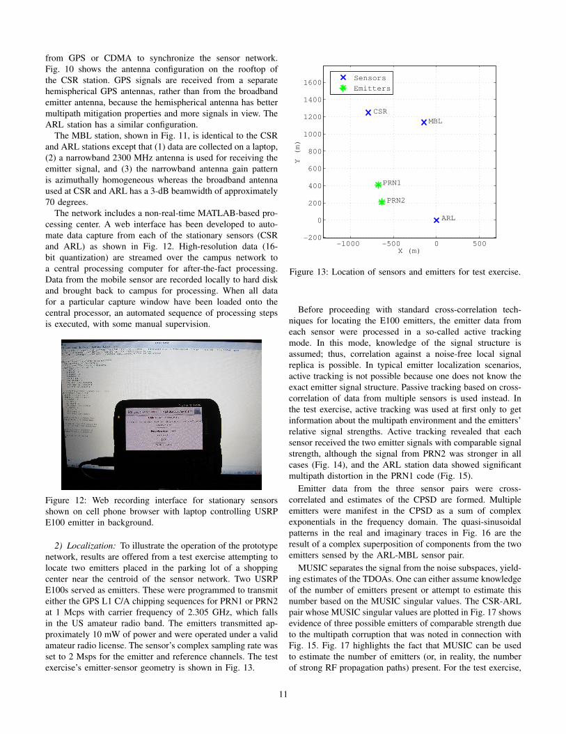
2) Localization: To illustrate the operation of the prototypenetwork, results are offered from a test exercise attempting tolocate two emitters placed in the parking lot of a shoppingcenter near the centroid of the sensor network. Two USRPE100s served as emitters. These were programmed to transmiteither the GPS L1 C/A chipping sequences for PRN1 or PRN2at 1 Mcps with carrier frequency of 2.305 GHz, which fallsin the US amateur radio band. The emitters transmitted ap-proximately 10 mW of power and were operated under a validamateur radio license. The sensor’s complex sampling rate wasset to 2 Msps for the emitter and reference channels. The testexercise’s emitter-sensor geometry is shown in Fig. 13.

−1000 −500 0 500−200

0

200

400

600

800

1000

1200

1400

1600

X (m)

Y (m)

Sensors

Emitters

MBL

CSR

PRN1

PRN2

ARL

Figure 13: Location of sensors and emitters for test exercise.

Before proceeding with standard cross-correlation tech-niques for locating the E100 emitters, the emitter data fromeach sensor were processed in a so-called active trackingmode. In this mode, knowledge of the signal structure isassumed; thus, correlation against a noise-free local signalreplica is possible. In typical emitter localization scenarios,active tracking is not possible because one does not know theexact emitter signal structure. Passive tracking based on cross-correlation of data from multiple sensors is used instead. Inthe test exercise, active tracking was used at first only to getinformation about the multipath environment and the emitters’relative signal strengths. Active tracking revealed that eachsensor received the two emitter signals with comparable signalstrength, although the signal from PRN2 was stronger in allcases (Fig. 14), and the ARL station data showed significantmultipath distortion in the PRN1 code (Fig. 15).

Emitter data from the three sensor pairs were cross-correlated and estimates of the CPSD are formed. Multipleemitters were manifest in the CPSD as a sum of complexexponentials in the frequency domain. The quasi-sinusoidalpatterns in the real and imaginary traces in Fig. 16 are theresult of a complex superposition of components from the twoemitters sensed by the ARL-MBL sensor pair.

MUSIC separates the signal from the noise subspaces, yield-ing estimates of the TDOAs. One can either assume knowledgeof the number of emitters present or attempt to estimate thisnumber based on the MUSIC singular values. The CSR-ARLpair whose MUSIC singular values are plotted in Fig. 17 showsevidence of three possible emitters of comparable strength dueto the multipath corruption that was noted in connection withFig. 15. Fig. 17 highlights the fact that MUSIC can be usedto estimate the number of emitters (or, in reality, the numberof strong RF propagation paths) present. For the test exercise,

11

(a) The GPS and 2300 MHz antenna are placed on top of the vehicle. (b) The USRP N200 RF recording equipment, power supply, andOCXO are placed inside the vehicle.

Figure 11: The MBL station is parked on top of a tall, nearby parking garage to ensure line-of-sight view of the emitters.

2.6 2.8 3 3.2 3.4 3.6 3.8 4

x 105

0

1

2

3

4

5

6x 10

9

Code Phase (m)

Correlation Power (front−end units)

PRN1

PRN2

Figure 14: Active tracking of GPS L1 C/A PRN codes in CSRdata reveals the presence of the two emitter signals.

it was assumed that the CSR-ARL and ARL-MBL sensor pairdetected three emitters and the CSR-MBL pair detected onlyone emitter, which seemed to best fit the data. Note that in theCSR-MBL pair, the TDOAs associated with the two emitterswere too closely spaced to be resolved given the SNRp in thistest exercise.

The estimated TDOAs must each be associated with a par-ticular emitter. This is done by examining the TDOA closuremetric which should be small when emitters are correctlyassociated. For the exercise, the closure threshold was sub-jectively chosen to be 100 m. Once a TDOA 3-tuple has beenassociated, emitters can then be precisely located at 3-wayhyperbolic intersection points. Hyperbolic trace estimates fromfive independent data segments are overlaid in Fig. 18 with1 s integration time. Fig. 19 shows the corresponding emitterlocation estimates, but because of the multipath corruption,three possible emitter locations are shown. Note that the

2.28 2.29 2.3 2.31 2.32 2.33

x 105

0

1

2

3

4

5

x 109

Code Phase (m)

Correlation Power (front−end units)

PRN1

PRN2

Figure 15: Active tracking of GPS L1 C/A codes in ARL datashows significant multipath distortion of the PRN1 code. Thepeak of the PRN2 code is outside the code phase window.

TDOA measurement resulting from the CSR-MBL sensor paircloses more than one 3-tuple of TDOAs, so it was assumedthat there could be an emitter at each of those intersections.

The location precision is about 20 m and the mean of onecluster of position estimates is within 10 m of a true emitter(PRN2). It is not known whether the other position clustersare associated with the other emitter (PRN1) or multipath.The absolute location accuracy is limited by not accountingfor the antenna heights of the sensors and emitters and thedifferential delay between the reference and emitter channeldue to 100s of feet of coaxial cable at the fixed sensors andfrequency-dependent biases in the USRP front end.

Note that if only one emitter is assumed to be present inthe received data, then the TDOA estimates become biasedand jump between different emitters as their strength variesas shown in Figs. 20 and 21. Clearly, multiple-emitter TDOA

12

−1 −0.5 0 0.5 1

x 106

−4

−2

0

2

4

6

8

10

12

14

16x 10

5

Frequency (Hz)

Power Density (frontend units)

real

imag

abs

weight

Figure 16: Cross power spectral density estimate for ARL-MBL pair based on 1 s of coherent averaging. Multipleemitters are manifest as a sum of complex exponentials inthe frequency domain. The light blue line indicates the boxcarfrequency weighting applied when estimating TDOAs for eachemitter.

0 5 10 15

103

104

105

106

107

singular value index

singular value

Figure 17: Singular values produced by the MUSIC algorithmfor the CSR-ARL pair. Assuming three emitters, the greenlines indicate the boundary of the signal subspace and the redlines indicate the boundary of the noise subspace. Note thatthere is a clear separation between the strongest noise singularvalue and the weakest signal singular value.

−1000 −500 0 500−200

0

200

400

600

800

1000

1200

1400

1600

X (m)

Y (m)

Sensors

Emitters

Hyperbolas

Figure 18: TDOA hyperbola map for the amateur band testexercise with an effective captured bandwidth of 1.5 MHz andintegration time of 1 s.

−1000 −500 0 500−200

0

200

400

600

800

1000

1200

1400

1600

X (m)

Y (m)

Sensors

True Emitters

Est. Emitters

Figure 19: Estimated emitter locations for five independentruns with 1 s coherent integration.

estimation techniques are required for accurate emitter local-ization.

VII. CONCLUSIONS

A full picture, from theory to hardware implementation withfield experiments, of a multiple-emitter localization systemis offered. A novel multi-reference synchronization strategybased on a tightly-coupled sensor architecture is adopted. Afocus on multiple emitters (as opposed to the single-emitterfocus of prior work on interference localization) leads to aTDOA estimation strategy based on parametric estimation

13

−1000 −500 0 500−200

0

200

400

600

800

1000

1200

1400

1600

X (m)

Y (m)

Sensors

Emitters

Hyperbolas

Figure 20: Hyperbolas generated by estimated TDOAs withthe single-emitter assumption and an integration time of 1 s.

−1000 −500 0 500−200

0

200

400

600

800

1000

1200

1400

1600

X (m)

Y (m)

Sensors

True Emitters

Est. Emitters

Figure 21: Estimated emitter locations with the single-emitterassumption and 1 s coherent integration.

techniques. The precision of the proposed TDOA estimatorapproaches the CRLB in a simulated representative scenario.Although the estimator becomes unreliable at low SNRp orfor closely-spaced emitters, it outperforms non-parametricmatched-filtering-based techniques. Field tests show 20 mlocalization precision for five independent runs. Multipath is asignificant challenge because it introduces false TDOA mea-surements that are consistent, leading to false emitter locationestimates. Future work will configure the prototype system todetect and localize emitters in the GNSS bands, explore UAV-based platforms to mitigate multipath and allow feedback-based, adaptive sensor network geometries, and modify the

processing algorithms to jointly estimate TDOA and FDOAin order to localize moving emitters.

ACKNOWLEDGMENT

This work was generously supported by Coherent Naviga-tion through a sponsored research agreement. The authors alsothank the members of the UT Radionavigation Laboratory.

REFERENCES

[1] National PNT Advisory Board, “Jamming the GlobalPositioning System - A national security threat: Recentevents and potential cures,” Nov. 2010.

[2] R. Mitch, R. Dougherty, M. Psiaki, S. Powell,B. O’Hanlon, J. Bhatti, and T. Humphrys, “Signal char-acteristics of civil GPS jammers,” in Proceedings ofthe ION GNSS Meeting, (Portland, Oregon), Institute ofNavigation, 2011.

[3] S. Pullen and G. Gao, “GNSS jamming in the name ofprivacy,” Inside GNSS, vol. 7, Mar./Apr. 2012.

[4] Department of Homeland Security official. private com-munication, Sept. 2011.

[5] Federal Communications Commission, “Public NoticeDA-05-1776,” June 2005.

[6] T. E. Humphreys, “The GPS dot and its discontents: Pri-vacy vs. GNSS integrity,” Inside GNSS, vol. 7, Mar./Apr.2012.

[7] B. Hamon and E. Hannan, “Spectral estimation of timedelay for dispersive and non-dispersive systems,” AppliedStatistics, pp. 134–142, 1974.

[8] E. Hannan and P. Thomson, “Estimating group delay,”Biometrika, vol. 60, no. 2, p. 241, 1973.

[9] C. Knapp and G. Carter, “The generalized correlationmethod for estimation of time delay,” Acoustics, Speechand Signal Processing, IEEE Transactions on, vol. 24,no. 4, pp. 320–327, 1976.

[10] A. Thompson, J. Moran, and G. Swenson, Interferometryand Synthesis in Radio Astronomy. Wiley, 2001.

[11] O. Isoz, A. T. Balaei, and D. Akos, “Interference detec-tion and localization in the GPS L1 band,” in Proceedingsof the ION ITM, (San Diego, CA), pp. 925–929, Instituteof Navigation, Jan. 2010.

[12] J. Lindstrom, D. M. Akos, O. Isoz, and M. Junered,“GNSS interference detection and localization using anetwork of low-cost front-end modules,” in Proceedingsof the ION GNSS Meeting, Institute of Navigation, 2007.

[13] K. G. Gromov, GIDL: Generalized Interference Detec-tion and Localization System. PhD thesis, StanfordUniversity, March 2002.

[14] M. B. Montminy, “Passive geolocation of low-poweremitters in urban environments using TDOA,” Master’sthesis, Air Force Institute of Technology, Mar. 2007.

[15] R. Schmidt, “Multiple emitter location and signal pa-rameter estimation,” Antennas and Propagation, IEEETransactions on, vol. 34, pp. 276 – 280, Mar. 1986.

[16] T. Sathyan, A. Sinha, and T. Kirubarajan, “Passive geolo-cation and tracking of an unknown number of emitters,”

14

Aerospace and Electronic Systems, IEEE Transactionson, vol. 42, pp. 740–750, April 2006.

[17] L. Scott, “J911: Fast Jammer Detection,” GPS World,vol. 21, no. 11, pp. 32–37, 2010.

[18] A. Brown, D. Reynolds, D. Roberts, and S. Serie, “Jam-mer and interference location system,” in Proceedingsof the ION GPS Meeting, (Nashville, TN), pp. 137–142,Institute of Navigation, Sept. 1999.

[19] A. Proctor, C. Curry, J. Tong, R. Watson, M. Greaves, andP. Cruddace, “Protecting the UK infrastructure,” InsideGNSS, vol. 6, Sep./Oct. 2011.

[20] K. Pesyna, Z. Kassas, J. Bhatti, and T. E. Humphreys,“Tightly-coupled opportunistic navigation for deep urbanand indoor positioning,” in Proceedings of the ION GNSSMeeting, (Portland, Oregon), Institute of Navigation,2011.

[21] A. Rihaczek, Principles of high-resolution radar.McGraw-Hill, 1969.

[22] M. Psiaki and S. Mohiuddin, “Modeling, analysis, andsimulation of GPS carrier phase for spacecraft relativenavigation,” Journal of Guidance Control and Dynamics,vol. 30, no. 6, p. 1628, 2007.

[23] K. M. Pesyna, Jr., K. Wesson, R. W. Heath, Jr., and T. E.Humphreys, “Extending the reach of GPS-assisted fem-tocell synchronization and localization through tightly-coupled opportunistic navigation,” in GLOBECOMWorkshops (GC Wkshps), 2011 IEEE, 2011.

[24] K. Wesson, K. Pesyna, J. Bhatti, and T. E. Humphreys,“Opportunistic frequency stability transfer for extendingthe coherence time of GNSS receiver clocks,” in Pro-ceedings of the ION GNSS Meeting, (Portland, Oregon),Institute of Navigation, 2010.

[25] T. E. Humphreys, B. M. Ledvina, M. L. Psiaki, andP. M. Kintner, Jr., “GNSS receiver implementation on aDSP: Status, challenges, and prospects,” in Proceedingsof the ION GNSS Meeting, (Fort Worth, TX), Institute ofNavigation, 2006.

[26] B. W. O’Hanlon, M. L. Psiaki, P. M. Kintner, Jr., andT. E. Humphreys, “Development and field testing of aDSP-based dual-frequency software GPS receiver,” inProceedings of the ION GNSS Meeting, (Savannah, GA),Institute of Navigation, 2009.

[27] T. E. Humphreys, J. Bhatti, T. Pany, B. Ledvina,and B. O’Hanlon, “Exploiting multicore technology insoftware-defined GNSS receivers,” in Proceedings ofthe ION GNSS Meeting, (Savannah, GA), Institute ofNavigation, 2009.

[28] B. O’Hanlon, M. Psiaki, S. Powell, J. Bhatti, T. E.Humphreys, G. Crowley, and G. Bust, “CASES: Asmart, compact GPS software receiver for space weathermonitoring,” in Proceedings of the ION GNSS Meeting,(Portland, Oregon), Institute of Navigation, 2011.

[29] A. Duel-Hallen, J. Holtzman, and Z. Zvonar, “Multiuserdetection for CDMA systems,” Personal Communica-tions, IEEE, vol. 2, pp. 46–58, April 1995.

[30] P. Madhani, P. Axelrad, K. Krumvieda, and J. Thomas,

“Application of successive interference cancellation tothe GPS pseudolite near-far problem,” Aerospace andElectronic Systems, IEEE Transactions on, vol. 39,pp. 481–488, April 2003.

[31] M. L. Psiaki, T. E. Humphreys, S. Mohiuddin, S. P.Powell, A. P. Cerruti, and J. Paul M. Kintner, “Searchingfor Galileo: Reception and analysis of signals fromGIOVE-A,” GPS World, vol. 17, pp. 66–72, June 2006.

[32] Y. Chan, R. Hattin, and J. Plant, “The least squaresestimation of time delay and its use in signal detection,”Acoustics, Speech and Signal Processing, IEEE Transac-tions on, vol. 26, pp. 217–222, June 1978.

[33] W. Bajwa, K. Gedalyahu, and Y. Eldar, “Identificationof parametric underspread linear systems and super-resolution radar,” Signal Processing, IEEE Transactionson, vol. 59, pp. 2548 –2561, June 2011.

[34] R. Roy and T. Kailath, “ESPRIT-estimation of signal pa-rameters via rotational invariance techniques,” Acoustics,Speech and Signal Processing, IEEE Transactions on,vol. 37, pp. 984–995, July 1989.

[35] J.-J. Fuchs, “Estimating the number of sinusoids inadditive white noise,” Acoustics, Speech and Signal Pro-cessing, IEEE Transactions on, vol. 36, pp. 1846–1853,Dec. 1988.

[36] A. Barabell, “Improving the resolution performanceof eigenstructure-based direction-finding algorithms,” inAcoustics, Speech, and Signal Processing, IEEE Interna-tional Conference on ICASSP ’83., vol. 8, pp. 336–339,April 1983.

[37] B. Rao and K. Hari, “Performance analysis of root-music,” Acoustics, Speech and Signal Processing, IEEETransactions on, vol. 37, pp. 1939–1949, Dec. 1989.

[38] Y. Chan and K. Ho, “A simple and efficient estimator forhyperbolic location,” Signal Processing, IEEE Transac-tions on, vol. 42, pp. 1905–1915, Aug. 1994.

15