development and use of operational modal analysis … · 27 may 2008 – development and use of...
TRANSCRIPT

DEVELOPMENT AND USE OF
OPERATIONAL MODAL ANALYSISExamples of Civil, Aeronautical and Acoustical Applications
Francesco Marulo – Tiziano [email protected]
27 27 MayMay 20082008StructuralStructural and and GeotechnicalGeotechnicalDynamicDynamic LaboratoryLaboratory STREGASTREGA
EngineeringEngineering FacultyFaculty -- University of MoliseUniversity of MoliseCampobasso Campobasso -- ItalyItaly
UniversitUniversitàà deglidegli StudiStudididi NapoliNapoli Federico IIFederico II

227 May 2008 – Development and Use of Operational Modal Analysis – F. Marulo and T. Polito
OverviewOverview
IntroductionIntroduction
TheoreticalTheoretical BackgroundBackground
NumericalNumerical assessmentassessment
Case Case StudiesStudies
DiscussionDiscussion of of ResultsResults
ConcludingConcluding RemarksRemarks
TypicalTypical ApplicationsApplications

327 May 2008 – Development and Use of Operational Modal Analysis – F. Marulo and T. Polito
IntroductionIntroduction
•• The operational modal analysis (OMA) is an added tool for the The operational modal analysis (OMA) is an added tool for the continuing improvement of the mancontinuing improvement of the man’’s productss products
•• Real time measurements and analysis represents an invaluable Real time measurements and analysis represents an invaluable process for gaining true experiences on structural dynamic process for gaining true experiences on structural dynamic behaviourbehaviour
OMA OMA advantagesadvantages:: OMA OMA drawbacksdrawbacks::
RealReal structuresstructures exhibitsexhibits truetruedynamicdynamic responseresponse
HypothesisHypothesis on the forcing on the forcing functionsfunctions
No No prepre--studiesstudies –– OnlyOnly retrofitretrofit
ExpertExpert useruser –– heavyheavy mathmath
427 May 2008 – Development and Use of Operational Modal Analysis – F. Marulo and T. Polito
Theoretical BackgroundTheoretical Background
[ ] ( ){ } [ ] ( ){ } [ ] ( ){ } ( ){ } [ ] ( ){ }tuDtFtxKtxCtxM ==++ &&&
maymay bebe writtenwritten asas::
kkkk
kkkk
vDuCxywBuAxx
++=++=+1
[ ] [ ] [ ][ ] [ ] [ ] [ ]⎟⎟⎠
⎞⎜⎜⎝
⎛−−
= −− CMKMI
Ac 11
0[ ] [ ] [ ]( )[ ] [ ]cc BAIAB 1−−=
[ ] [ ][ ] [ ]⎟⎟⎠
⎞⎜⎜⎝
⎛= − BM
Bc 1
0
( )tkxxk Δ=
( )tAA cΔ= exp
wherewhere
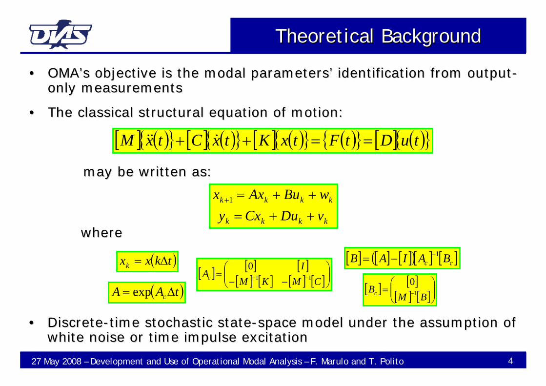
•• OMAOMA’’ss objective is the modal parametersobjective is the modal parameters’’ identification from outputidentification from output--only measurementsonly measurements
•• The classical structural equation of motion:The classical structural equation of motion:
•• DiscreteDiscrete--time stochastic statetime stochastic state--space model under the assumption of space model under the assumption of white noise or time impulse excitationwhite noise or time impulse excitation

527 May 2008 – Development and Use of Operational Modal Analysis – F. Marulo and T. Polito
HankelHankel matrixmatrix
⎡ ⎤⎢ ⎥⎢ ⎥⎢ ⎥⎢ ⎥⎢ ⎥⎢ ⎥⎣ ⎦
a b c d eb c d e fc d e f gd e f g he f g h i
•• A A HankelHankel matrix is a square matrix that is symmetric and constant matrix is a square matrix that is symmetric and constant across the antiacross the anti--diagonalsdiagonals
•• HankelHankel matrices are formed when given a sequence of output data matrices are formed when given a sequence of output data and a realization of an underlying stateand a realization of an underlying state--space or hidden Markov space or hidden Markov model is desired. model is desired.
•• The Singular Value Decomposition (SVD) of the The Singular Value Decomposition (SVD) of the HankelHankel matrix matrix provides a means of computing the A,B, and C matrices which defiprovides a means of computing the A,B, and C matrices which define ne the statethe state--space realization space realization

627 May 2008 – Development and Use of Operational Modal Analysis – F. Marulo and T. Polito
•• Data Driven (DD)Data Driven (DD)
This algorithm is based on the following definition of the This algorithm is based on the following definition of the HankelHankelmatrixmatrix
Methods for OMAMethods for OMA
⎟⎟⎠
⎞⎜⎜⎝
⎛=⎟
⎟⎠
⎞⎜⎜⎝
⎛=
⎟⎟⎟⎟⎟⎟⎟⎟⎟⎟⎟
⎠
⎞
⎜⎜⎜⎜⎜⎜⎜⎜⎜⎜⎜
⎝
⎛
=−
−
−+−
+++
−++
−+−
−
f
refp
ii
refi
Niii
Niii
Niii
refNi
refi
refi
refN
refref
refN
refref
ref
YY
YY
yyy
yyyyyyyyy
yyyyyy
NH
12|
1|0
22212
21
11
21
21
110
...............
...
...
...............
...
...
1
which projects future outputs into the space of the past outpuwhich projects future outputs into the space of the past outputsts
•• Again the singular value decomposition provides, through the Again the singular value decomposition provides, through the observabilityobservability and controllability matrices, the structural modal and controllability matrices, the structural modal parametersparameters

727 May 2008 – Development and Use of Operational Modal Analysis – F. Marulo and T. Polito
Methods for OMA Methods for OMA (cont(cont’’dd))
[ ][ ] [ ] [ ][ ] [ ] [ ]
[ ] [ ] [ ]⎥⎥⎥⎥⎥
⎦
⎤
⎢⎢⎢⎢⎢
⎣
⎡
=
−++
+
11
132
21
,
qppp
q
q
qp
RRR
RRRRRR
H
L
LLLL
L
L
whichwhich, , eventuallyeventually through a through a weightingweighting processprocess, can , can bebe realizedrealizedin the in the observabilityobservability and and controllabilitycontrollability matricesmatrices
ChoiceChoice of the of the weightingweighting matricesmatrices maymay help help forfor ananimprovedimproved system system identificationidentification
[ ] { }{ }∑−−
=+−
=1
0
1 kS
s
Trefsskk yy
kSR
[ ][ ][ ] [ ] [ ][ ] [ ] [ ][ ] [ ]
[ ][ ]
[ ][ ][ ]TT
T
qp VSUVVS
UUWHW 1112
11212,1 00
0=⎥
⎦
⎤⎢⎣
⎡⎥⎦
⎤⎢⎣
⎡=
•• Covariance Data Driven (CDD)Covariance Data Driven (CDD)
Based on the Based on the HankelHankel matrix built asmatrix built as

827 May 2008 – Development and Use of Operational Modal Analysis – F. Marulo and T. Polito
InIn--house Software house Software AMOpAMOp
•• DevelopedDeveloped in the in the MatlabMatlab©© environmentenvironment•• Text format for the input data files (different sources)Text format for the input data files (different sources)•• Useful for both novice and expert userUseful for both novice and expert user
Sta
rtin
gSta
rtin
gsc
reen
scre
en
Sta
biliz
atio
nSta
biliz
atio
ndi
agra
mdi
agra
mGeometryGeometrymodulemodule

927 May 2008 – Development and Use of Operational Modal Analysis – F. Marulo and T. Polito
Numerical SimulationNumerical Simulation
6 6 dofdof’’s s systemsystem
ResponseResponse toto ImpulseImpulse ExcitationExcitation
ResultsResults
ReferenceValues
17.7227 0.0101
33.2686 0.1191
36.0597 0.1242
46.6333 0.0538
64.5757 0.0001
78.2414 0.3103
nf nξ
ResponseResponse toto RandomRandom ExcitationExcitation
•• The numerical simulation appears to be a viable tool for checkinThe numerical simulation appears to be a viable tool for checking g the algorithms and the developed softwarethe algorithms and the developed software

1027 May 2008 – Development and Use of Operational Modal Analysis – F. Marulo and T. Polito
Numerical ResultsNumerical Results
RobustRobust methodologymethodology
ReferenceValues
17.7227 33.2686 36.0597 46.6333 64.5757 78.2414
0.0101 0.1191 0.1242 0.0538 0.0001 0.3103
Impulse Exc. Random Exc.
AMOpCDD
17.7208 0.0790 16.8556 0.0259
33.2341 0.1161 34.9262 0.1580
36.0521 0.1215 35.6151 0.1212
46.6298 0.0520 48.1198 0.0529
64.5776 0.0001 64.5817 0.0001
78.2288 0.3091 89.0154 0.3489
Impulse Exc. Random Exc.
AMOpDD
17.7227 0.0101 16.8801 0.0266
33.2686 0.1191 35.0807 0.1209
36.0597 0.1242 37.0801 0.0330
46.6333 0.0538 46.8852 0.0541
64.5757 0.0001 66.2111 0.0000
78.2414 0.3103 80.2832 0.3503
nξ
nf
nf nξ nf nξnf nf nξnξ

1127 May 2008 – Development and Use of Operational Modal Analysis – F. Marulo and T. Polito
Simulation of a Real StructureSimulation of a Real Structure
0 0.5 1 1.5 2 2.5 3 3.5 4 4.5 5-8
-6
-4
-2
0
2
4
6x 10⁻⁸
Am
plitu
de
time [sec]
Grid Point #3 - Acceleration Time History
0 0.5 1 1.5 2 2.5 3 3.5 4 4.5 5-2.5
-2
-1.5
-1
-0.5
0
0.5
1
1.5
2
2.5x 10
-7
Am
plitu
de
time [sec]
Grid Point #10 - Acceleration Time History
CloseClose toto excitationexcitation Far Far fromfrom excitationexcitation
•• Finite element analysis of a bridgeFinite element analysis of a bridge
•• Modal parameters easily computed numericallyModal parameters easily computed numerically
•• Simulation with impulse forcing functionSimulation with impulse forcing function

1227 May 2008 – Development and Use of Operational Modal Analysis – F. Marulo and T. Polito
Flight TestingFlight Testing
To establish variation of the modal parameters with speed
ObjectiveObjective::
•• In Flight measurement of the vertical fin & rudder vibration behIn Flight measurement of the vertical fin & rudder vibration behaviouraviour
Pilot induced excitation through pedals mixed with air turbulence
Input Force:Input Force:

1327 May 2008 – Development and Use of Operational Modal Analysis – F. Marulo and T. Polito
Flight Test ResultsFlight Test Results
180 km/h
DD 4.25 0.641 11.75 0.028 24.24 0.039 33.20 0.018
CDD 4.74 0.731 11.80 0.043 NI NI 32.81 0.030
200 km/h
DD 3.96 0.280 11.65 0.038 28.96 0.020 NI NI
CDD 3.91 0.440 11.75 0.058 28.51 0.052 NI NI
220 km/h
DD 3.73 0.600 11.81 0.023 25.05 0.163 NI NI
CDD 4.45 0.630 11.83 0.032 25.85 0.320 NI NI
f [Hz] ξ f [Hz] ξ f [Hz] ξ f [Hz] ξ
mode 1 mode 2 mode 3
mode 4
mode 4
Rudder & Fin - Test Case A
mode 1 mode 2 mode 3
mode 1 mode 2 mode 3 mode 4
ResultsResults
V=180 Km/hV=180 Km/h
V=220 Km/hV=220 Km/h
FinFin RudderRudder
InputInput
•• Example of measured acceleration timeExample of measured acceleration time--historieshistories

1427 May 2008 – Development and Use of Operational Modal Analysis – F. Marulo and T. Polito
Testing on Civil StructuresTesting on Civil Structures
Traffic excitationTraffic excitation Step bumper truckStep bumper truck
Freq. [Hz] Damp. [%]
DD CDD DD CDD
0,89 0,91 0,04 0,04
1,15 1,20 0,03 0,04
2,44 2,03 0,05 0,06
3,01 2,95 0,04 0,04
3,75 3,65 0,06 0,06
11stst
33rdrd
•• Bridge deck motorwayBridge deck motorwayIdentification of the first structural modeIdentification of the first structural mode--shapes shapes
(model correlation, structural monitoring, (model correlation, structural monitoring, ……))

1527 May 2008 – Development and Use of Operational Modal Analysis – F. Marulo and T. Polito
Acoustic ApplicationAcoustic Application
FacilityFacility forfor the the measurementmeasurement of the of the
TransmissionTransmission LossLoss (TL) of (TL) of StructuralStructural
PanelsPanels
•• SMallSMall Acoustic Research Facility (SMARF)Acoustic Research Facility (SMARF)

1627 May 2008 – Development and Use of Operational Modal Analysis – F. Marulo and T. Polito
Receiving RoomReceiving Room
RunRun 4 4 –– ModalModal HammerHammerRunRun 5 5 –– ModalModal HammerHammerRunRun 6 6 –– SpeakerSpeaker
RunRun 1 1 –– SpeakerSpeakerRunRun 2 2 –– ModalModal HammerHammerRunRun 3 3 –– ModalModal HammerHammer
MicrophoneMicrophone SetupSetup #1#1 MicrophoneMicrophone SetupSetup #2#2

1727 May 2008 – Development and Use of Operational Modal Analysis – F. Marulo and T. Polito
AMOpAMOp ApplicationApplication
•• Examples of Stabilization DiagramsExamples of Stabilization Diagrams

1827 May 2008 – Development and Use of Operational Modal Analysis – F. Marulo and T. Polito
Num Num –– Exp CorrelationExp Correlation
OMA vs. FEM Comparison OMA vs. FEM Comparison –– Receiving RoomReceiving Room

1927 May 2008 – Development and Use of Operational Modal Analysis – F. Marulo and T. Polito
Soundproofing EffectSoundproofing Effect
RunRun 7 7 –– Speaker (Speaker (withoutwithout soundproofingsoundproofing))RunRun 8 8 –– Speaker (Speaker (withwith soundproofingsoundproofing))
MicrophoneMicrophone SetupSetup #3#3Time history comparison with and without soundproofing treatmentTime history comparison with and without soundproofing treatment

2027 May 2008 – Development and Use of Operational Modal Analysis – F. Marulo and T. Polito
Damping BehaviorDamping Behavior
•• OMA computed damping tendency with and without soundproofing walOMA computed damping tendency with and without soundproofing wall l treatmenttreatment

2127 May 2008 – Development and Use of Operational Modal Analysis – F. Marulo and T. Polito
ConclusionsConclusions
•• Operational Modal Analysis is an important tool, eventually the Operational Modal Analysis is an important tool, eventually the only only one, for the structural identification of real structureone, for the structural identification of real structure
•• Two correlationTwo correlation--driven stochastic subspace techniques have been used driven stochastic subspace techniques have been used on both simulated and real measurementson both simulated and real measurements
•• Efficiency of the methodology even in high modal density environEfficiency of the methodology even in high modal density environmentment
•• Good ability and coherence in identifying the damping behaviourGood ability and coherence in identifying the damping behaviour
•• It may need an expert user, for a correct interpretation of the It may need an expert user, for a correct interpretation of the input input data and identified resultsdata and identified results
•• More reliable results are generally obtained combining all the aMore reliable results are generally obtained combining all the available vailable information on the tested structure, properly information on the tested structure, properly weightedweighted