development, evaluation, and application of a food web
TRANSCRIPT

DEVELOPMENT, EVALUATION, AND APPLICATION OF A FOOD WEB BIOACCUMULATION MODEL FOR PCBs
IN THE STRAIT OF GEORGIA, BRITISH COLUMBIA
Colm David Condon B.Sc., University of British Columbia, 1997
A PROJECT SUBMITTED IN PARTIAL FULFILLMENT OF THE REQUIREMENTS FOR THE DEGREE OF
MASTER OF RESOURCE MANAGEMENT
In the School
of Resource and Environmental Management
O Colm David Condon 2007
SIMON FRASER UNIVERSITY
Spring 2007
All rights reserved. This work may not be reproduced in whole or in part, by photocopy
or other means, without permission of the author.
APPROVAL
Name:
Degree:
Title of Research Project:
Report No.:
Examining Committee:
Date Approved:
Colm David Conclon
Master of Resource Management
Development, Evaluation, and Application of a Food Web Bioaccumulation Model for PCBs in the Strait of Georgia, British Columbia
Dr. Frank A.P.C. Gobas Senior Supervisor Professor
School of Resource and Environmental Management S~mon Fraser University
Dr. Peter S. Ross Adjunct Professor
Simon Fraser University

SIMON FRASER :b~ d UN~VERS~TY l i bra r y
DECLARATION OF PARTIAL COPYRIGHT LICENCE
The author, whose copyright is declared on the title page of this work, has granted to Simon Fraser University the right to lend this thesis, project or extended essay to users of the Simon Fraser University Library, and to make partial or single copies only for such users or in response to a request from the library of any other university, or other educational institution, on its own behalf or for one of its users.
The author has further granted permission to Simon Fraser University to keep or make a digital copy for use in its circulating collection (currently available to the public at the "Institutional Repository" link of the SFU Library website <www.lib.sfu.ca> at: ~http:llir.lib.sfu.calhandlell8921112~) and, without changing the content, to translate the thesislproject or extended essays, if technically possible, to any medium or format for the purpose of preservation of the digital work.
The author has further agreed that permission for multiple copying of this work for scholarly purposes may be granted by either the author or the Dean of Graduate Studies.
It is understood that copying or publication of this work for financial gain shall not be allowed without the author's written permission.
Permission for public performance, or limited permission for private scholarly use, of any multimedia materials forming part of this work, may have been granted by the author. This information may be found on the separately catalogued multimedia material and in the signed Partial Copyright Licence.
The original Partial Copyright Licence attesting to these terms, and signed by this author, may be found in the original bound copy of this work, retained in the Simon Fraser University Archive.
Simon Fraser University Library Burnaby, BC, Canada
Revised: Spring 2007
ABSTRACT
In an effort to enhance the understanding of persistent organic pollutant (POP)
bioaccumulation in the Strait of Georgia, I developed, parameterized, and tested a
mechanistic bioaccumulation model for polychlorinated biphenyls (PCBs) in the Strait of
Georgia. Review of the literature required to support the model uncovered significant
gaps in the empirical dataset. These gaps limit the usefulness of the model as a
management tool; however, enough data were available to support analysis of the current
sediment quality guideline for PCBs in British Columbia. This analysis suggests that the
guideline is inadequate to protect top predators in the Strait of Georgia and may not meet
the Ministry of Environment's protection objectives. I recommend that research be
directed at improving the empirical database required for bioaccumulation modelling in
the Strait of Georgia and that bioaccumulation models similar to that developed here be
used when deriving sediment quality guidelines for other POPS.
Keywords: bioaccumulation; biomagnification; PCBs; Strait of Georgia; food web;
sediment quality guidelines
. . . I l l

ACKNOWLEDGEMENTS
I sincerely thank Frank Gobas, my senior supervisor, for sharing with me (through his
course and this project) some of his deep and broad knowledge of contaminant science
and policy with a style that made it surprisingly comprehensible. I sincerely thank Peter
Ross for his speedy review of this document and for sharing his food web knowledge and
seal data. I sincerely thank the following researchers for also sharing their data and
knowledge without which this project would not have been possible: John Elliott, Jim
West & Sandra O'Neil, Robie Macdonald, David Carpenter, Richard Beamish, Ryan
Stevenson, and Jon Arnot. I sincerely thank the Natural Sciences and Engineering
Research Council of Canada (NSERC), Environment Canada, and Vancity Credit Union
(through its environmental scholarship) for providing research funds throughout my
studies. I sincerely thank all the teachers, staff, and students at REM (especially
members of the Gobas research group), who leave me with many fond memories and a
deeper understanding of the world around me. I sincerely thank the Ministry of
Environment for allowing me to take occasional leaves from work to finish this paper.
Finally, I sincerely thank my family, friends, and Barri for their support throughout the
demanding journey that has led to completion of my MRM degree.

TABLE OF CONTENTS
. . Approval ............................................................................................................................. 11
... ............................................................................................................................. Abstract 111
........................................................................................................... Acknowledgements iv
.............................................................................................................. Table of Contents v . . .................................................................................................................. List of Figures VII
List of Tables ...................................................................................................................... x . . Glossary ............................................................................................................................ xu
............................................................................................................ List of Acronyms xiv
1 Introduction ................................................................................................................ 1 ........................................................................................................... 1.1 Background 1
1.2 Risk Management ................................................................................................. 2 1.2.1 Georgia Basin Action Plan ........................................................................... 3
............................................................................... 1.2.2 Ministry of Environment 3 1.3 Project Objectives ................................................................................................. 4
............................................................................................................... 1.4 Overview 5
2 Bioaccumulation Theory ....................................................................................... 8 2.1 Overview ............................................................................................................... 8 2.2 Bioaccumulation Description - Water Breathers & Plants .................................. 9
................................................. 2.3 Bioaccumulation Description - Birds and Seals 17 ................................................................. 2.4 Seal Pup & Bird Egg Concentrations 23
............................................................................ 2.5 Water and Air Concentrations 24
3 Methods ..................................................................................................................... 27 ............................................................................................. 3.1 BSAF Calculations 27
3.1.1 Calculation Tools ......................................................................................... 27 3.1.2 SoG Food Web Structure ............................................................................. 27 3.1.3 Model Parameterization ............................................................................... 32
.................................................................... 3.1.4 Selection of PCB Congeners 33 ..................................... 3.1.5 Input and Performance Analysis Data ... ................. 35
3.1.6 Data Gaps and BSAF Prediction Implications ........................................... 39 ........................................................................... 3.2 Model Performance Analysis 43
3.2.1 Comparison of Predicted and Observed BSAFs ................................... 4 3 3.2.2 MB Calculations and Analysis .................................................................... 43 3.2.3 Data Gaps and Model Performance Analysis Implications ......................... 44
3.3 Model Application .............................................................................................. 47 3.3.1 Overview ..................................................................................................... 47
3.3.2 Ecological Risk Assessment for Top Predators ........................................... 47 .................. 3.3.3 Sediment Quality Guideline Evaluation and Recommendation 51
3.3.4 Sediment Quality Target Proposals ............................................................. 53 ......................................... 3.3.5 Data Gaps and Model Application Implications 53
4 Results & Discussion ............................................................................................. 56 .............................................................................. 4.1 Accuracy of the Diet Matrix 56
4.2 BSAF Predictions for CPCBs ........................................................................... 58 .............................................................................. 4.3 Model Performance Analysis 59
...................................... 4.3.1 Model Performance Analysis for PCB Congeners 60 ................................................... 4.3.2 Model Performance Analysis for CPCBs 77
.............................................................. 4.3.3 Performance Analysis Uncertainty 78 ............................................................................................. 4.4 Model Application 78
4.4.1 Ecological Risk Assessment ........................................................................ 79 .................. 4.4.2 Sediment Quality Guideline Evaluation and Recommendation 83
............................................................. 4.4.3 Sediment Quality Target Proposals 89
5 Conclusions & Recommendations ......................................................................... 91 ................................................................................................. 5.1 Project Summary 91
........................................................................... 5.2 Key Findings and Implications 93 ............................................................................................... 5.3 Recommendations 94
6 Appendices ............................................................................................................... 99 6.1 Diet Matrix Verification Data ............................................................................. 99
.................................................................................. 6.2 Seal and Bird kM Values 102 ............................................................................. 6.3 Empirical Model Input Data 103
6.4 Model Parameter Values ................................................................................ 106 ............................................................................... 6.5 Model Sensitivity Analysis 120
................................................................... 6.6 Model Perfolmance Analysis Data 125 ...................................................................................... 6.7 CD Copy of the Model 126
References ...................................................................................................................... 127
LIST OF FIGURES
Figure 1-1 Figure 1-2
Figure 2- 1 Figure 2-2 Figure 2-3
Figure 3 - 1
Figure 3-2
Figure 4- 1
Figure 4-2 Figure 4-3
Figure 4-4
Figure 4-5
Figure 4-6
Figure 4-7
....................................... Map of the Strait of Georgia and surrounding area 1
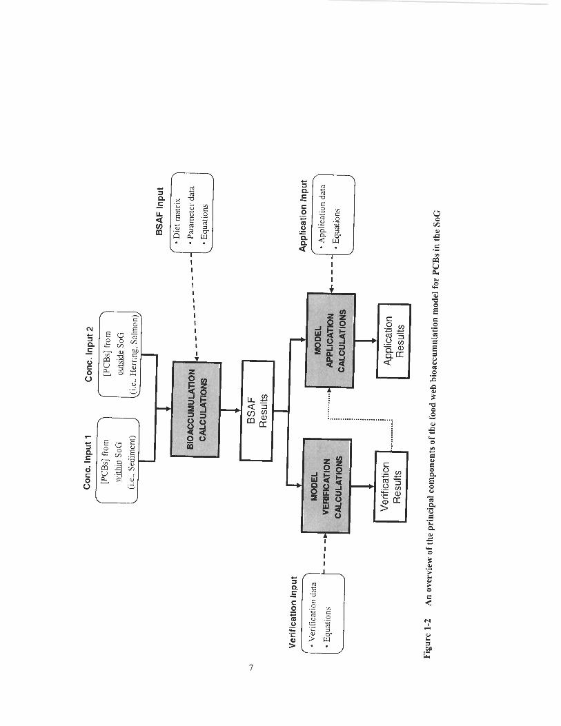
An overview of the principal components of the food web ................................................ bioaccumulation model for PCBs in the SoG 7
............ PCB uptake and elimination pathways for phytoplankton and algae 9 ............... PCB uptake and elimination pathways for invertebrates and fish 10
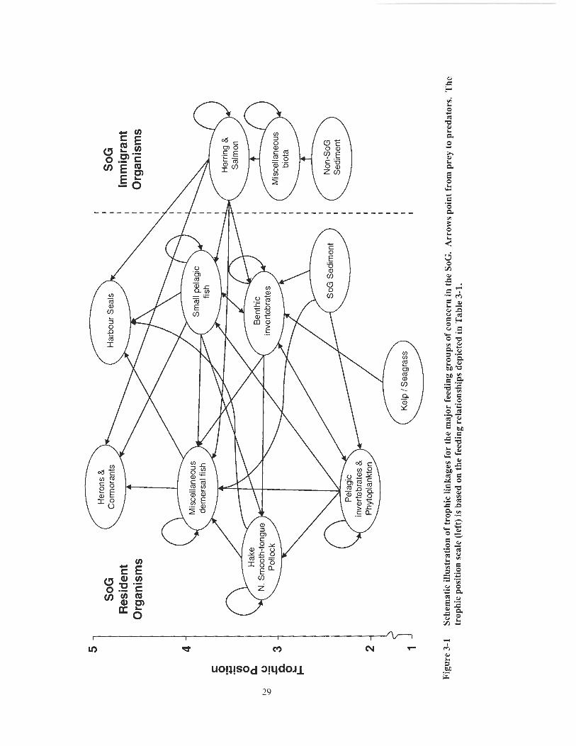
.......................... PCB uptake and elimination pathways for birds and seals 18 Schematic illustration of trophic linkages for the major feeding groups of concern in the SoG. Arrows point from prey to predators. The trophic position scale (left) is based on the feeding relationships depicted in Table 3-1. .............................................................................. 29 Sampling locations in the SoG for model input and model performance analysis data. .......................................................................... 36
Correlation between tropic position and 6I5N isotope ratios for select organisms. 6 " ~ values and references are presented in Table 6-3 (see Appendices). ....................................................................................... 57 Predicted BSAFs for CPCB in all modelled organisms of the SoG ............ 59
Predicted and observed BSAFs (g-wet-organism 1 g-dry-sediment) of various PCB congeners in adult female seals from the SoG. Error bars represent two standard deviations of the observed geometric mean (n = 4) ............................................................................................... 61 Predicted and observed BSAFs (g-wet-organism / g-dry-sediment) of various PCB congeners in seal pups from the SoG. Error bars represent two standard deviations of the observed geometric mean (n - - 10). ...................................................................................................... 6 2
Predicted and observed BSAFs (g-wet-organism 1 g-dry-sediment) of various PCB congeners in cormorant eggs from the SoG. Error bars represent two standard deviations of the observed geometric mean (n= 19). ............................................................................................... 63 Predicted and observed BSAFs (g-wet-organism / g-dry-sediment) of vaiious PCB congeners in heron eggs from the SoG. Error bars represent two standard deviations of the observed geometric mean (n - - ................................ ........................................................................ 12). .... 64 Predicted and observed BSAFs (g-wet-organism / g-dry-sediment) of various PCB congeners in dogfish from the SoG. Error bars
vii

represent two standard deviations of the observed geometric mean (n - - 9) .............................................................................................................. 65
Figure 4-8 Predicted and observed BSAFs (g-wet-organism 1 g-dry-sediment) of various PCB congeners in English sole from the SoG. Error bars represent two standard deviations of the observed geometric mean (n - - 9) ............................................................................................................... 66
Figure 4-9 Predicted and observed BSAFs (g-wet-organism 1 g-dry-sediment) of various PCB congeners in miscellaneous demersal fish (seal prey) from the SoG. Error bars represent two standard deviations of the observed geometric mean (n = 5). ............................................................... 67
Figure 4- 10 Predicted and observed BSAFs (g-wet-organism / g-dry-sediment) of various PCB congeners in miscellaneous de~nersal fish (bird prey) from the SoG. Error bars represent two standard deviations of the observed geometric mean (n = 5). ............................................................. 68
Figure 4- 1 1 Predicted and observed BSAFs (g-wet-organism / g-dry-sediment) of various PCB congeners in shellfish from the SoG. Error bars represent two standard deviations of the observed geometric mean (n - - 4). .............................................................................................................. 69
Figure 4- 12 Predicted and observed BSAFs (g-wet-organism 1 g-dry-sediment) of various PCB congeners in crabs fi-om the SoG. Error bars represent two standard deviations of the observed geometric mean (n - - 9) ............................................................................................................... 70
Figure 4- 13 Comparison of the ratio of predicted (P) and observed (0) BSAF values to log-Kow values, on a congener-specific basis, for modelled top predators of the SoG. SF = adult female seals, SP = seal pups, CE = cormorant eggs, and HE = heron eggs. .............................................. 76
Fibwre 4-14 Predicted and observed BSAFs (glg) of CPCBs for seal pups, adult female seals, cormorant eggs, and heron eggs from the SoG, Error bars represent two standard deviations of the observed geometric mean (n = 10 for seal pups, 4 for adult female seals, 19 for cormorant eggs, and 12 for heron eggs) ..................................................... 77
Figure 4-1 5 The predicted and observed distribution (n = 4) of CPCB concentrations (nglg lipid) in adult female seats in relation to the effects threshold. The solid and dashed curves depict the predicted and observed CPCB distributions, respectively. The horizontal dotted line marks the effects threshold. The circled value indicates the proportion of adult female seals in the SoG predicted to have CPCB concentrations above the threshold. ................................................. 79
Figure 4- 16 The predicted and observed distribution (n = 10) of CPCB concentrations (nglg lipid) in seal pups in relation to the effects threshold. The solid and dashed curves depict the predicted and observed CPCB distributions, respectively. The horizontal dotted line marks the effects threshold. The circled value indicates the

proportion of seal pups in the SoG predicted to have CPCB concentrations above the threshold ........................... ... ................................ 8 1
Figure 4- 17 The predicted and observed distribution of CPCB concentrations (ng/g lipid) in cormorant eggs in relation to the LOAEL. The solid and dashed curves depict the predicted and observed CPCB distributions, respectively. The horizontal dotted line marks the LOAEL. ....................................................................................................... 82
Figure 4- 18 The CPCB concentration predicted from the current SQG (as indicated by the blue arrow on each graph) for adult female seals [A], seal pups [B], and cormorant eggs [C], relative to their TRVs and predicted (solid lines) and observed (dashed lines) CPCB distributions. ............................................................................................ 85
Figure 4- 19 The CPCB concentration distribution predicted by multiplying the current SQG by the observed (dashed line) and predicted (solid line) BSAFs for adult female seals [A] and coimorant eggs [B] relative to their TRVs. .................................................................................................. 87
............................................. Figure 6- 1 Results of sensitivity analysis for seal pups 122 Figure 6-2 Results of sensitivity analysis for adult male seals .................................... 122 Figure 6-3 Results of sensitivity analysis for cormorant eggs .................................... 123 Figure 6-4 Results of sensitivity analysis for heron eggs ............................................ 123
LIST OF TABLES
Table 3- 1
Table 3-2
Table 3-3 Table 3-4 Table 3-5
Table 3-6
Table 3-7 Table 4- 1
Table 4-2 Table 4-3
Table 4-4
Table 4-5
Table 6- 1
Table 6-2
Table 6-3
Table 6-4 Table 6-5
Table 6-6
A matrix of diet compositions (% wet weight) for select organisms of the SoG. Values represent annual averages ......................................... 30 PCB Congeners Reported in the Model Input and Top Predator Verification Datasets. ........................................................................ 34 Summary of model input and performance analysis data ............................ 35
A summary of data gaps and BSAF prediction implications ...................... 40 A summary of data gaps and model performance analysis implications ...................................... .. ................................................... 45
PCB congeners used to calculate the seal TRVs and the CPCB concentration distributions for model-predicted seals, observed adult female seals, and observed seal pups used in the ERA ............................... 50 A summary of data gaps and model application implications ..................... 54 Individual and combined MB results (i.e., mean, lower 95%, and upper 95%) for select organisms of the SoG (i.e., those with a performance analysis dataset) on a congener-specific basis ....................... 7 1
Correlation data for Figure 4- 13 ............................................................ 76 MB results for adult female seals, cormorant eggs, and heron eggs on a CPCBs basis ........................................................................................ 78
Comparison of current and recommended SQGs for CPCBs (pglg- OC). ...... .. . . . . . .. . . . . . .. . . . . . . . . . . . . . . . ... , . . . , . . . . . . . , , . . . , . . , , . . . , . . , , . . . , . . . , . . . . . . . . . . . . . . . . , . . . . . . . . . . . . . 88
Proposed sediment quality targets for CPCBs (yglg-OC) for the protection of seals and marine birds in the SoG. ......................................... 90 The estimated annual average diet of harbour seals in the SoG [from Olesiuk, 19931 ................. .... .. .. .... .. .... . .. . . . . . . . . . . . . . . . . . . . . . . . 99 SoG diet matrix reported in Pauly & Christensen, 1995 ........................... 100
Calculated TPs and literature derived 6'" ratios for organisms of the SoG feeding matrix ................................................................. ... ... .. ... 10 1
Estimated seal and bird kM values ........................................................ 102 Empirical sediment data used as model input (n = 3). Congener numbers in bold were included in the dataset provided by R. Macdonald; congener numbers in brackets are the co-eluting congeners assumed to be represented by the numbers in bold. ................. 103 Empirical herring data used as model input (n = 2) .................................. 104
Table 6-7
Table 6-8 Table 6-9 Table 6- 10 Table 6-1 1 Table 6- 12 Table 6- 13 Table 6- 14
Table 6- 1 5 Table 6- 16 Table 6- 17 Table 6- 1 8 Table 6- 19
Empirical salmon data used as model input (n = 3 for all salmon species) ..................................................................................................... 105 Values for PCB congener properties used in the model ............................ 106 Environmental parameter definitions. values. and references ................... 107 General biological parameter definitions. values. and references ............. 108 Plant parameter definitions. values. and references .................................. 109 Invertebrate parameter definitions. values. and references ....................... 110 Fish parameter definitions. values. and references .................................... 113 Double-crested Cormorant parameter definitions. values. and references ................................................................................................... 117 Great Blue Heron parameter definitions. values. and references .............. 118 Harbour seal parameter definitions. values. and references ...................... 119 Organism legend for sensitivity analysis figures ...................................... 121 Empirical bird data used to verify model predictions ............................. 125
Empirical seal data used to verify model predictions ................................ 126

GLOSSARY
TERM DEFINITION REFERENCE
Bioaccumulation
Bioaccumulation factor
Biomagnification
Biota-sediment accumulation factor
Ecological risk assessment
Equilibrium
Fugacity capacity
The process by which the chemical concentration within an organism achieves a level that exceeds that in its environment as a result of chemical uptake through all possible routes of exposure (e.g., dietary, dermal, respiratory).
The ratio of the chemical concentration in the organism to the chemical concentration in the water. The concentration can be expressed on a wet weight, dry weight, or lipid weight basis.
The process in which the chemical concentration in an organism achieves a level that exceeds that in the organism's diet, due to dietary absorption.
The ratio of the chemical concentration in an organism to the chemical concentration in the sediment in which the organism resides.
Ecological risk assessment is a process that evaluates the likelihood that adverse ecological effects are occurring or may occur as a result of exposure to one or more stressors
A condition where the chemical's potentials (also chemical activities and fugacities) are equal in the environmental media. At equilibrium, chemical concentrations in static environmental media remain constant over time.
The proportionality constant that indicates the abilitv of a media to absorb a solute and varies
Gobas & Morrison, 2000
Gobas & Morrison, 2000
Gobas & Morrison, 2000
Gobas & Morrison, 2000
US EPA, 1992
Gobas & Morrison, 2000
Mackay, 1991
with ihe nature of the chemical and the
xii

Lowest observed adverse effect limit
No observed adverse effect limit
Octanol-air partition coefficient
Octanol-water partition coefficient
Persistent organic pollutant
Trophic position
medium, the temperature, pressure, and concentration.
The lowest concentration or dose in a test which produced an observable adverse effect.
The maximum concentration or dose in a test which produces no observed adverse effects.
The ratio of a chemical's solubility in octanol vs. air.
The ratio of a chemical's solubility in octanol vs. water.
A chemical possessing three primary attributes: persistence, tendency to bioaccumulate, and toxicity
A condition where the total flux of chemical into an organism equals the total flux out with no net change in mass or concentration of the chemical.
A measure of an organism's trophic status in a food web which, by providing non-integer quantities, considers the effects of omnivory, cannibalism, feeding loops, and scavenging on
US EPA, 2006
US EPA, 2006
Derived from Mackay, 1991
Mackay, 1991
Wania & Mackay 1999
Gobas & Morrison, 2000
Vander Zanden & Rasmussen, 1996
food web structure.

LIST OF ACRONYMS
BAF
BC
BSAF
COSEWlC
DSL
dw
ERA
GB
GBAP
KO A
Kow
LOAEL
MB
MOE
NLOM
NOAEL
OC
PBDEs
PCBs
EPCBs
POPS
SoG
Bioaccumulation factor
British Columbia
Biota-sediment accumulation factor
Committee on the Status of Endangered Wildlife in Canada
Domestic Substances List
Dry weight
Ecological risk assessment
Georgia Basin
Georgia Basin Action Plan
Octanol-air partition coefficient
Octanol-water partition coefficient
Lowest observed adverse effects level
Model bias
BC Ministry of Environment
Non-lipid organic matter
No observed adverse effects level
Organic carbon
Polybrominated diphenyl ethers
Polychlorinated biphenyls
Total polychlorinated biphenyls
Persistent organic pollutants
Strait of Georgia
xiv

SQG
SQT
TP
TRV
WW
Sediment Quality Guideline
Sediment Quality Target
Trophic position
Toxicity reference value
Wet weight

1 INTRODUCTION
1.1 Background
The Strait of Georgia (SoG), which lies in south-westem British Columbia (BC) within
the Georgia Basin (GB) (Figure 1-l), is home to a rich and complex food web and one of
the largest estuaries in North America.
Adapttd fiom Copyright 0 Province of British Columbia. All lights rcse~vcd. Reprinl with pcnnission of the Province of B~itisli Columbia. www.ipp.gov.bc.ca
Figure 1-1 Map of the Strait of Georgia and sorrosuding area

The SoG is also home to approximately eight million surrounding residents who, through
their various cominercial and recreational activities, exert considerable stress on the SoG
ecosystem. One of the contributing stressors is the presence of persistent organic
pollutants (POPs) that originate locally, regionally, and globally. POPs of particular
concern include polychlorinated biphenyls (PCBs), polybrominated diphenyl ethers
(PBDEs), polychlorinated dibenzo-p-dioxins (PCDDs), and others. Many of the 209
highly stable, persistent PCB congeners, for instance, are known to bioaccumulate up
aquatic food webs and are believed to disrupt endocrine function, suppress the immune
system, and impair reproduction in a wide range of biota including fish, marine
mammals, birds, and humans [Van den Berg et al., 1998; Newsted et al., 1995; Ross et
crl . , 20001.
Recent SoG monitoring studies have detected high levels of PCBs in wild and farmed
salmon [Hites et al., 20041, double-crested and pelagic cormorant eggs [Harris et al.,
20051, great blue heron eggs [Harris et al., 20031, harbour seals [Ross ct al., 20041, and
orcas [Ross et a/., 20001. In fact, PCB levels are so high in southern resident and
transient orcas (an average of 150 and 250 mglkg lipid, respectively) that these organisms
are considered among the most PCB-contaminated cetaceans in the world [Ross et al.,
20001. Studies have also detected high concentrations of PBDEs, polybrominated
biphenyls (PBBs), and polychlorinated naphthalenes (PCNs) in transient and resident
orcas [Rayne et al., 20041.
1.2 Risk Management
The investigation and management of potential risks to SoG wildlife associated with
exposure to POPs is a key concern for two institutions: the Georgia Basin Action Plan
(GBAP) and the BC Ministry of Environment (MOE). The roles of each are discussed
below.

1.2.1 Georgia Basin Action Plan
The Georgia Basin Action Plan (GBAP) is a multi-partnered initiative (i.e., including
various federal, provincial, and municipal government agencies, non-governmental
organizations, private corporations, etc.) that is working to improve sustainability in the
Georgia Basin [Environment Canada, 20051. Among the GBAP's many goals is the aim
of improving the capacity of environmental managers to make decisions by advancing
scientific understanding [Environment Canada, 20051. For example, to help
environmental managers manage POP-exposure risks to GB wildlife, Environment
Canada (EC) is funding the development of mass balance models aimed at improving
scientific understanding of POP-pollution dynamics in the SoG. These models will
simulate the flux of POPs into and out of the environmental media of the SoG over time
and relate POP concentrations in environmental media to POP concentrations in, and
associated risks to, resident wildlife of the SoG.
The POP mass balance models are expected assist environmental risk managers in a
number of ways. For example, they will help them to (i) set POP emissions targets that
meet desired ecological risk endpoints (e.g., no more than 10% of the harbour seal
population with PCB body burdens that exceed their effects threshold for PCBs); (ii)
predict the response time of the SoG to POP reduction strategies; (iii) identify which
POPs on the Domestic Substances List (DSL) should be targeted for management or
virtual elimination (as per Environment Canada, 2004); (iv) prioritize research aimed to
better achieve GBAP objectives; etc.
1.2.2 Ministry of Environment
The BC Ministry of Environment (MOE) manages the exposure of wildlife to chemicals
primarily by setting environmental quality guidelines. BC's ambient sediment quality
guidelines (SQGs), for instance, "apply province-wide and are safe levels of substances
for the protection of a given water use, including drinking water, aquatic life, recreation
and agricultural uses" [MOE, 20061.

Currently, SQGs exist for only two POPs: PCBs and PAHs. SQGs for dioxins and furans
are under development, and SQGs for other POPs are expected in the coming years. The
SQG for CPCBs is based on a combination of (i) PCB exposure and effects data from
laboratory studies conducted primarily on freshwater fish and invertebrates, (ii) the
application of simple equilibrium partitioning equations, and (iii) the application of
uncertainty factors [Nagpal, 19921. Given that little, if any, SoG-specific data was used
to derive the SQG for CPCBs, and given the high potential for PCB biomagnification in
the SoG food web (note its complexity in Table 3-1) and the high concentrations of PCBs
in SoG wildlife (particularly orcas), it is unclear whether the current SQG for CPCBs is
sufficient to meet the MOE's protection objectives.
1.3 Project Objectives
To help improve POP-associated risk management in BC, I have conducted a research
project with the following objectives:
1. Develop, parameterize, and test a food web bioaccumulation model for PCBs that
estimates biota sediment accumulation factors (BSAFs) for a set of resident
organisms of the SoG. This model is intended to form all or part of the biological
component of a broader fate model for PCBs in the SoG. It is also intended to
serve as a foundation for the biological component of mass balance models
developed in the future for other POPs (including PBDEs). I elected to use PCBs
in this initial food web model because empirical datasets for PCBs (e.g., congener
properties, environmental and biological concentrations, etc.), which are
necessary for performance analysis and application, are much more
comprehensive for PCBs than for other POPs. In addition, PCBs are easier to
model than some other POPs because they are poorly (or not) metabolized by fish,
invertebrates, algae, and other lower-trophic organisms. not metabolized by
lower-trophic organisms.
2. Use this model to

characterize the risks to top predators of the SoG associated with current
levels of PCB exposure,
characterize the level of protection offered to top predators of the SoG by the
current SQG for ZPCBs,
propose a new SQG for ZPCBs which meets the MOE's protection goals, and
propose sediment quality targets (SQTs) for CPCBs which protect top
predators of the SoG to various risk-related endpoints (e.g., not more than 5%
of cormorant eggs above the no observed adverse effects level (NOAEL), 5%
of seal pups above the effects threshold, etc.).
3. Use the literature review required for the model to identify PCB bioaccumulation
data gaps and make research recommendations aimed at narrowing these gaps.
1.4 Overview
A conceptual overview of the tood web bioaccumulation model is presented below
(Figure 1-2). Rounded-corner white boxes indicate major inputs; grey boxes indicate
calculation routines; and sharp-corner white boxes indicate major outputs. The model
can be viewed as having three basic components. The first is the bioaccumulation
calculation component, where I coi~vert measured, congener-specific concentrations of
PCBs in SoG sediments, herring, and salmon to predicted, congener-specific PCB-
BSAFs for 3 1 organisms/organism groups in the SoG. The second is the model
performance analysis component, where I compare model predicted BSAFs to
empirically derived BSAFs. The third is the model application component, where, upon
satisfactory completion of the model performance analysis, I use the model to address
various issues of environmental management interest.
The following paper details each of the components introduced above. The
bioaccumulation routines used to predict organism BSAFs are described in the
bioaccumulation theory section. The methods used to derive the BSAF, performance

analysis, and application results are described, in turn, in the methods section. And the
results of the BSAF, performance analysis, and application phases are described and
discussed, in turn, in results and discussion section.
2 BIOACCUMULATION THEORY
2.1 Overview
The ultimate aim of the model's bioaccumulation equations is to generate congener-
specific BSAFs (dg) for resident organisms and organism groups in the SoG. BSAFs
relate sediment and organism concentrations as per the following equation:
C B = BSAF * Cs PI
where CB (ng/g-ww) is the PCB congener concentration in the biological organism, and
Cs (ng/g-dw) is the PCB congener concentration in sediment.
To derive BSAFs, the model converts, through the application of literature derived mass-
balance equations, empirical PCB congener concentrations in SoG sediment to predicted
PCB congener concentrations in SoG organisms. This approach has been applied
successfully in a number of other systems including San Francisco Bay, Lake Ontario,
and Kitimat Arm [Gobas & Amot, 2005; Gobas et nl., 1998; Morrison et al., 1997;
Stevenson, 2003; etc.]. Sections 3.2 to 3.5 (below) describe the bioaccumulation
equations. I divide the description into (i) a general bioaccumulation equation for marine
phytoplankton, algae, invertebrates, and fish and (ii) a general bioaccumulation equation
for birds and seals. The derivation of equations is not included (refer to Amot & Gobas,
2004 and Gobas & Amot, 2005 for these details) except where 1 have developed
equations specific to this system.
2.2 Bioaccumulation Description - Water Breathers & Plants
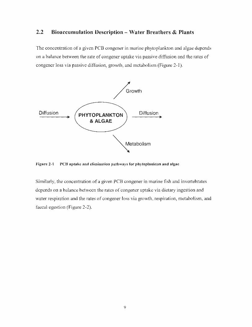
The concentration of a given PCB congener in marine phytoplankton and algae depends
on a balance between the rate of congener uptake via passive diffusion and the rates of
congener loss via passive diffusion, growth, and metabolism (Figure 2-1).
Growth / Diffusion Diffusion ,
& ALGAE
Metabolism \ Figure 2-1 PCB uptake and eliminatiou pathways for phytoplankton and algae
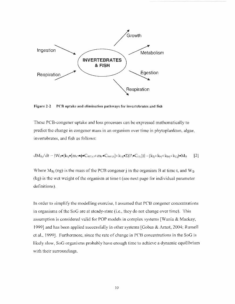
Similarly, the concentration of a given PCB congener in marine fish and invertebrates
depends on a balance between the rates of congener uptake via dietary ingestion and
water respiration and the rates of congener loss via growth, respiration, metabolism, and
faecal egestion (Figure 2-2).
Growth / / INVERTEBRATES \
Figure 2-2 PCB uptake and elimination pathways for invertebrates and fish
These PCB-congener uptake and loss processes can be expressed mathematically to
predict the change in congener mass in an organism over time in phytoplankton, algae,
invertebrates, and fish as follows:
Where Mgi (ng) is the mass of the PCB congener j in the organism B at time t, and WB
(kg) is the wet weight of the organism at time t (see next page for individual parameter
definitions).
In order to simplify the modelling exercise, I assumed that PCB congener concentrations
in organisms of the SoG are at steady-state (i.e., they do not change over time). This
assumption is considered valid for POP models in complex systems [Wania & Mackay,
19993 and has been applied successfully in other systems [Gobas & Arnot, 2004; Russell
et al., 19991. Furthermore, since the rate of change in PCB concentrations in the SoG is
likely slow, SoG organisms probably have enough time to achieve a dynamic equilibrium
with their surroundings.

Assuming steady-state (i.e., dMB/dt = 0), equation 2 rearranges to predict the PCB
congener concentration in an organism as follows:
Where
= concentration of congener j in the organism (ng/g wet weight)
= rate of congener j uptake via respiration (d-1)
= fraction of the respiratory ventilation that involves overlying water (unitless)
= fraction of the respiratory ventilation that involves pore water (unitless)
= fraction of congener j in overlying water that can be absorbed (unitless)
= total concentration of congener j in overlying water (ng/mL)
= freely dissolved concentration of congener j in pore water (ng/mL)
= rate of congener j uptake via dietary ingestion (d-1)
= fraction of the diet consisting of prey item i (unitless)
= concentration of congener j in prey item i (g/kg)
= rate of congener j elimination via respiration (d-1)
= rate of congener j elimination via egestion (d-1)
= rate of congener j elimination via metabolic transformation (d-1)
= rate of congener j elimination via growth (d-1)
For phytoplankton and algae, kD, kE, and kM are assumed to equal zero and equation 3
simplifies to the following:
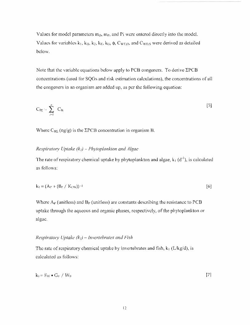
Values for model parameters mo, mp, and Pi were entered directly into the model.
Values for variables k l , kD, kZ, kE, kG, @, C W T , ~ , and CwDs were derived as detailed
below.
Note that the variable equations below apply to PCB congeners. To derive CPCB
concentrations (used for SQGs and risk estimation calculations), the concentrations of all
the congeners in an organism are added up, as per the following equation:
Where CBZ (ndg) is the CPCB concentration in organism B.
Respiratory Uptake (k,) - Phytoplankton and Algae
The rate of respiratory chemical uptake by phytoplankton and algae, k l (d-'), is calculated
as follows:
Where Ap (unitless) and Bp (unitless) are constants describing the resistance to PCB
uptake through the aqueous and organic phases, respectively, of the phytoplankton or
algae.
Respiratory Uptake (k,j - Invertebrates and Fish
The rate of respiratory chemical uptake by invertebrates and fish, kl (Llkdd), is
calculated as follows:
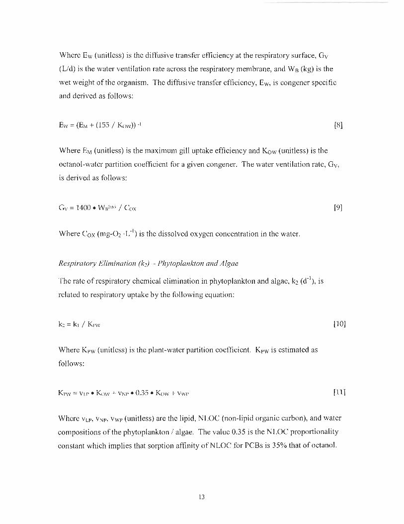
Where EW (unitless) is the diffusive transfer efficiency at the respiratory surface, Gv
(Lld) is the water ventilation rate across the respiratory membrane, and WB (kg) is the
wet weight of the organism. The diffusive transfer efficiency, Ew, is congener specific
and derived as follows:
Ew = (EM + (155 / Kow)) -' PI
Where EM (unitless) is the maximum gill uptake efficiency and Kow (unitless) is the
octanol-water partition coefficient for a given congener. The water ventilation rate, Gv,
is derived as follows:
Where Cox (mg-O2 +L- ' ) is the dissolved oxygen concentration in the water.
Respiratoiy Elimiization (k?) - Phytoplankton and Algae
The rate of respiratory chemical elimination in phytoplankton and algae, k2 (d-I), is
related to respiratory uptake by the following equation:
Where KpW (unitless) is the plant-water partition coefficient. KpW is estimated as
follows:
Where vl,p, VNP, VWP (unitless) are the lipid, NLOC (non-lipid organic carbon), and water
compositions of the phytoplankton / algae. The value 0.35 is the NLOC proportionality
constant which implies that sorption aftinity of NLOC for PCBs is 35% that of octanol.

Respimtoi-y Elimination (kz) -Invcrtcbi.atcs a id Fish
The rate of chemical elimination via respiration in invertebrates and fish, k;? (d"), is
related to respiratory uptake as follows:
Where KBW (unitless) is the biota-water partition coefficient. Partitioning between biota
and water of the SoG is a hnction of the fiaction of lipid, non-lipid organic matter
(NLOM), and water in the organism as described by the following equation:
KUIY = VI.B Knw + VNR P KOW + VWB
Where VLB, VNB, and VWB (unitless) are the lipid, NLOM, and water fraction of the
organism, respectively, and P (unitless) is the NLOM proportionality constant which
relates the PCB sorption capacity of NLOM to lipids. A P value of 0.035 was used (see
parameterization section below) implying that sorption affinity of NLOM for PCBs is
3.5% that of octanol.
Dietary Uptake (IrDj - Inver.tebmtes arid Fish
The rate at which PCBs are absorbed from the diet, kD (d-') is estimated as follows:
Where ED (unitless) is the dietary chemical transfer efficiency, GD (kg/d) is the feeding
rate, and WB (kg) is the wet weight of the organism. ED was estimated using the
following two-phase resistance model:

Where EDA and EDB are species-specific constants (see parameterization section for
values). The feeding rates, GD, for filter feeders and detritovores are estimated
respectively as
Where Gv (Lld) is the water ventilation rate (described above), Vss (kdL) is the
concentration of suspended solids in the water, o (unitless) is the particle scavenging
efficiency, and TW (K) is the water temperature.
Faecal Elimination (kE) - Invertebrates and Fish
The rate of chemical elimination by egestion, kE (dm'), is derived as follows:
Where GF (kg-faeceslkg-organismld) is the faecal egestion rate, ED (unitless) is the
dietary chemical transfer efficiency (described above), KCiB (unitless) is the gut-biota
partition coefficient, and WB (kg) is the wet weight of the organism. GF is estimated as
follows:
Where EL, EN, and EW (unitless) are the dietary absorption efficiencies of lipid, NLOM,
and water, respectively; VLD, VND, and VWD (unitless) are lipid, NLOM, and water
composition of the diet, respectively; and GD (kg/d) is the feeding rate (described above).
The gut-biota partition coefficient, KGB (unitless), is estimated as follows:

Where ZGUr (mol/m3-pa) is the fugacity capacity (or chemical sorptive capacity) of the
organism's gut contents, and ZoRG (mol/m3-pa) is the fugacity capacity of the organism.
ZGUr is estimated from the following equation:
Where VLG, VNG, and VWG (unitless) are the lipid, NLOM, and water contents,
respectively, of the organism's gut contents; ZL and Zw (mol/m3-pa) are the fugacity
capacities of lipid and water, respectively; and P (unitless) is the NLOM proportionality
constant. The sum of the VLG, VNG, and VWG approach 1 and are estimated as follows:
ZL and Z\V are estimated by the following equations:
Where KO* (unitless) is the octanol-air partition coefficient, R (pa-m3/mol K) is the ideal
gas constant, and T (K) is the water temperature (lower trophic organisms) organism
temperature (seals and birds).
The fugacity capacity of the organism, ZORG, is estimated as follows:

Where VLB, VNB, and v w ~ (unitless) are the lipid, NLOM, and water composition of the
organism, respectively, and ZL and ZW (mol/m3-pa) are the fugacity capacities of lipid
and water, respectively (described above).
Growth Dilution (kc) - All Lower. Tt-ophic Organisms
The rate of chemical dilution by growth, kG (d-'), for phytoplankton and algae is input
directly (see parameter section) and for invertebrates and fish is derived from the
following equation:
Where GRF (unitless) is the species-specific growth rate factor.
Metabolic Elimincrtion (kIk,j - All Lower Trophic Organisms
The rate of chemical elimination via metabolism, kM (d"), is assumed to be zero for lower
trophic organisms.
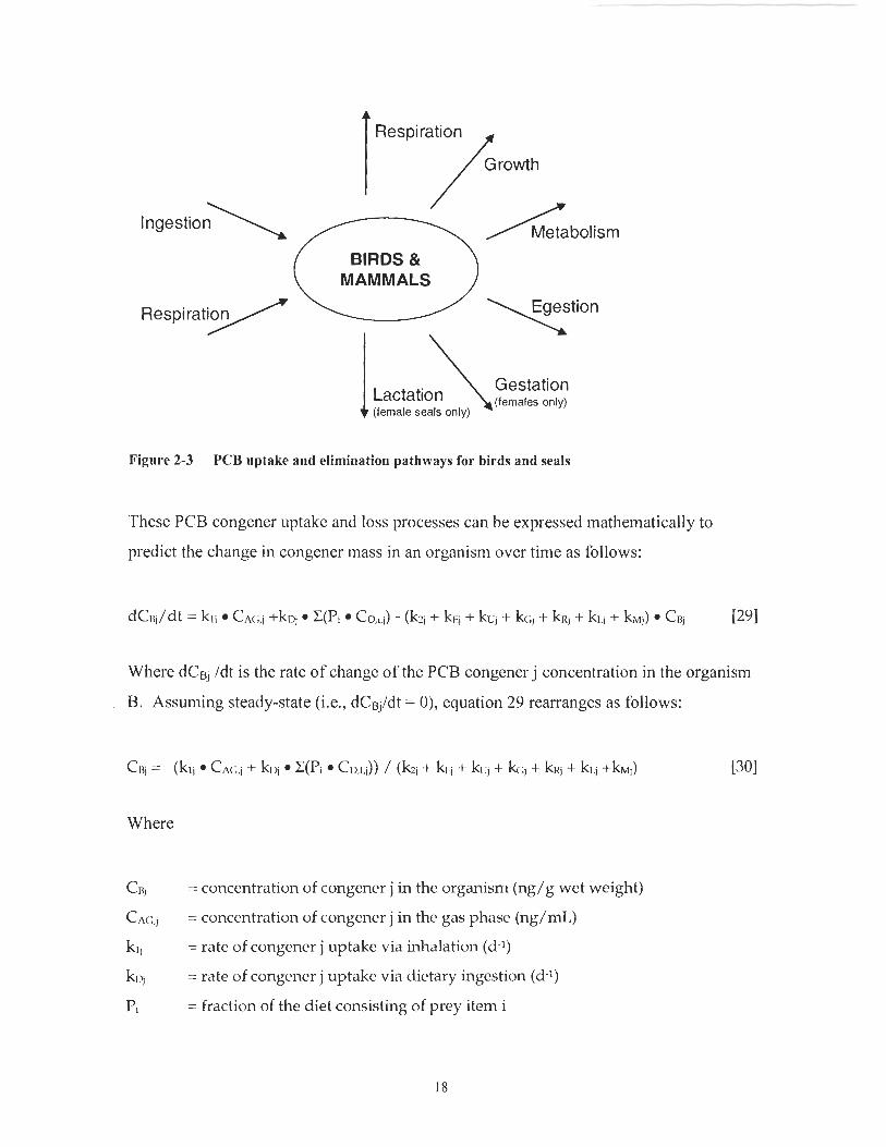
2.3 Bioaccumulation Description - Birds and Seals
The concentration of a given PCB congener in marine birds and seals depends on the
balance between the rates of chemical uptake via dietary ingestion and air respiration and
the rates of chemical loss via respiration, growth, metabolism, faecal egestion, gestation
(females only) and lactation (female seals only) (Figure 2-3).
Respiration
Growth / Ingestion\
BIRDS & MAMMALS
~ e s ~ i r a t i y
Lactation (females only) (female seals only)
Figure 2-3 PCB uptake and eliminatiou pathways for birds and seals
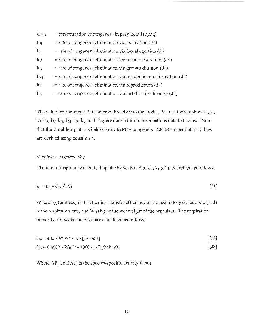
These PCB congener uptake and loss processes can be expressed mathematically to
predict the change in congener mass in an organism over time as follows:
Where dCBj /dt is the rate of change of the PCB congener j concentration in the organism
B. Assuming steady-state (i.e., dCBj/dt = O), equation 29 rearranges as follows:
Where
C I ~ = concentration of congener j in the organism (ng/g wet weight)
C A ~ = concentration of congener j in the gas phase (ng/mL)
kl, = rate of congener j uptake via inhalation (d-1)
k~ ? = rate of congener j uptake via dietary ingestion (d-1)
Pi = fraction of the diet consisting of prey item i
= concentration of congener j in prey item i (ng/g)
= rate of congener j elimination via exhalation (d-1)
= rate of congener j elimination via faecal egestion (d-1)
= rate of congener j elimination via urinary excretion (d-1)
= rate of congener j elimination via growth dilution (d-1)
= rate of congener j elimination via metabolic transformation (d-1)
= rate of congener j elimination via reproduction (d-1)
= rate of congener j elimination via lactation (seals only) (d-1)
The value for parameter Pi is entered directly into the model. Values for variables kl, kD,
k2, kE, ku, kG, kM, kR, kL, and CaqG are derived from the equations detailed below. Note
that the variable equations below apply to PCB congeners. CPCB concentration values
are derived using equation 5.
Respiratory Uptakc (1cJ
The rate of respiratory chemical uptake by seals and birds, k l (d-I), is derived as follows:
Where EA (unitless) is the chemical transfer efficiency at the respiratory surface, GA (Lld)
is the respiration rate, and WB (kg) is the wet weight of the organism. The respiration
rates, GA, for seals and birds are calculated as follows:
GI-\ = 480 W#75 AF @r seals]
GA = 0.4089 WHO," 1000 AF Vor birds]
Where AF (unitless) is the species-specific activity factor.
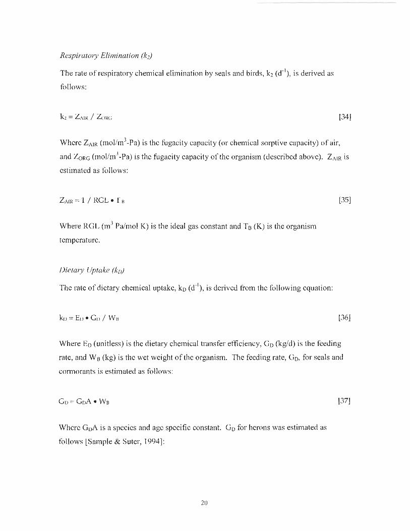
Respiratory Elimination (1c2)
The rate of respiratory chemical elimination by seals and birds, k2 (d-I), is derived as
follows:
Where Z A l ~ (mol/m3-pa) is the fugacity capacity (or chemical sorptive capacity) of air,
and Z O R ~ (mol/m3-pa) is the fugacity capacity of the organism (described above). ZAIR is
estimated as follows:
Where RGL (m3 Palm01 K) is the ideal gas constant and TB (K) is the organism
temperature.
Dietary Uptake (kl$
The rate of dietary chemical uptake, kD (d-I), is derived from the following equation:
Where ED (unitless) is the dietary chemical transfer efficiency, GD (kdd) is the feeding
rate, and We (kg) is the wet weight of the organism. The feeding rate, GD, for seals and
cormorants is estimated as follows:
Where GDA is a species and age specific constant. GD for herons was estimated as
follows [Sample & Suter, 19941:

Faecal Elimination (kE)
The rate of chemical elimination by egestion, kE (d-I), for seals and birds is derived in the
same way as that for invertebrates and fish (see above).
Urinary Elirnirzation (krJ
The rate of chemical elimination by urination, kU (d-I), is derived as follows:
ku = (Gu / WI~) En (Zw / ZORG)
Where Gu (L / d) is the urination rate, WB (kg) is the wet weight of the organism, ED
(unitless) is the chemical transfer eftjciency (described above), and Zw and ZoRG
(mol/m3-pa) are the fugacity capacities of water and the organism, respectively
(described above). The urination rates, Gu, for seals and birds are calculated as follows:
GU = 0.33 GF (seals)
GU = 0.2 GF (birds)
Where GF (kg-faeceslkg-organismld) is the faecal egestion rate (described above).
Growth Dilutiorz @(;)
The rate of chemical elimination by growth dilution for seals and birds is based on
empirical data (see parameterization section).
Rcpt.oductive Elimination (kn) - Seals
The rate of PCB elimination via reproduction, kR (d-'), is derived for adult female seals
from the following equation:

Where ZF and ZM (mol/m3-pa) are the fugacity capacities of the foetus and mother,
respectively; WF and WM (kg) are the wet weights of the foetus and mother, respectively;
and PR (unitless) is the proportion of the seal population reproducing. ZF and ZM are
estimated with the ZoRG equation (see above).
Reproductive Elimination (lid - Birds
The rate of PCB elimination via reproduction, kR (d-I), is derived for female birds from
the following equation:
Where ZE and ZM (mol/m3-pa) are the fugacity capacities of the egg and mother,
respectively; WE and WM (kg) are the wet weights of the egg and mother, respectively;
and NEC and NCY are the number of eggs per clutch and number of clutches per year,
respectively. ZE and ZM are estimated with the ZoRG equation (see above)
Lactntional Elimination (Ii[)
The rate of PCB elimination via lactation, kL (d-I), is only applicable to adult female seals
and is derived from the following equation:
Where ZMILK and ZM (mol/m3-pa) are the fugacity capacities of the milk and mother,
respectively; GD (Lld) is the feeding rate of the pup (described above); and WM (kg) is
the wet weight of the mother. ZMILK and ZM are derived using the Z o k ~ equation (see
above).

Metabolic Elimination (k,+b
Though PCB metabolism has been observed for some congeners in harbour seals [Boon
et al., 1987, 1994, 19971 and birds [Drouillard ct a/., 20011, I found no equations in the
literature describing the rate of PCB elimination via metabolism, kM (d-'), for these
organisms. To derive congener-specific kM values for cormorants, herons, and harbour
seals, I calibrated the model to fit empirical PCB concentration data as per Boon et al.,
1994, 1997; Gobas and Arnot, 2005. Specifically, I (a) calculated the concentration ratio
of PCB-X : PCB- 153 (where PCB-X is one of the 209 PCB congeners and PCB-1 53 is a
non-metabolized congener) in the empirical datasets for cormorant eggs, heron eggs, and
adult female seals, and (b) adjusted the value of kM in the model until the predicted PCB-
X : PCB- 153 ratio matched that of the observed. The kM values derived for female seals
were used for all seals, while kM values derived for bird eggs were used for adult birds.
The results are included in the appendices (Table 6-4). Note that the estimated kM values
are similar to those calculated for the San Francisco Bay [Gobas & Arnot, 20051 and
derived from laboratory studies [Drouillard et a]., 20011. For instance, the kM values for
PCB-37 and PCB-99 are relatively high and relatively low, respectively, my model and
the literature.
2.4 Seal Pup & Bird Egg Concentrations
Seal pups take up and eliminate PCBs via the same routes as seal adults (i.e., oral
ingestion, inhalation, exhalation, egestion, etc.), except that their only source of dietary
intake is mother's milk. I used the following equation to estimate the concentration of
PCB congeners in seal pups (ngg):
Where the subscript j denotes the congener of interest, k l (d-') is the respiratory uptake
rate constant (described above); CAG (ndmL) is the PCB concentration in the gas phase;
kD (d-') is the dietary uptake rate constant (described above); ZMILK (mol/m3-Pa) is the
fugacity capacity of milk (described above); ZM (mol/m3-pa) is the fugacity capacity of

the mother seal (described above); CM (nglg) is the wet weight PCB concentration in the
mother; and kEL.IM (d-I) is the sum of the pup's elimination rate constants.
Heron and connorant eggs get their PCB load solely from their mother as well. I used the
following equation to estimate the concentration of PCBs in bird eggs:
Where the subscript j denotes the congener of interest, ZEGG (mol/m3-pa) is the fugacity
capacity of the egg, ZM (mol/m3-pa) is the fugacity capacity of the mother (described
above), and CM is the PCB concentration in the mother. ZEGG was calculated using the
ZoRG equation (described above).
2.5 Water and Air Concentrations
To predict PCB concentrations in biota of the SoG, I required PCB concentrations in
sediments, water, and air of the SoG (see equations 3 and 30). Empirical data was
available for sediment only, so I estimated the PCB concentrations in water and air from
the sediment concentration data as detailed below.
Concentration of Dissolved PCBs in Water (Cry,))
I used the following equation to estimate the dissolved water concentrations of PCB
congeners, CwD, (ng/mL), in the SoG:
Where the subscript j denotes the congener of interest, Cs (ng/g) is the concentration of
the PCB congener in sediment, $oc (unitless) is the organic carbon content of sediment,
6ocs (kdL) is the density of organic carbon in sediment, Kow (unitless) is the saltwater
adjusted octanol-water partition coefficient, and FIoc (unitless) is the organic carbon
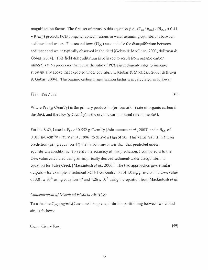
magnification factor. The first set of terms in this equation (i.e., (Csj 1 Qoc) 1 ( 6 0 ~ s 0.41
Kowi)) predicts PCB congener concentrations in water assuming equilibrium between
sediment and water. The second term (lloc) accounts for the disequilibrium between
sediment and water typically observed in the field [Gobas & MacLean, 2003; deBruyn &
Gobas, 20041. This field disequilibrium is believed to result froin organic carbon
mineralization processes that cause the ratio of PCBs in sediment-water to increase
substantially above that expected under equilibrium [Gobas & MacLean, 2003; deBruyn
& Gobas, 20041. The organic carbon magnification factor was calculated as follows:
Where PpR ( g - ~ i c m ~ l y ) is the primary production (or formation) rate of organic carbon in
the SoG, and the Boc (g-~/cm2/y) is the organic carbon burial rate in the SoG.
For the SoG, I used a P ~ R of 0.552 g -~ /cm2/y [Johannessen et al., 20031 and a Boc of
0.01 1 g - ~ / c r n ~ / y [Pauly et al., 19961 to derive a not of 50. This value results in a Cwo
prediction (using equation 47) that is 50 times lower than that predicted under
equilibrium conditions. To verify the accuracy of this prediction, I compared it to the
CwD value calculated using an empirically derived sediment-water disequilibrium
equation for False Creek [Mackintosh et al., 20061. The two approaches give similar
outputs - for example, a sediment PCB-1 concentration of 1.0 nglg results in a CwD value
of 3.8 1 x 10" using equation 47 and 4.26 x lo-' using the equation from Mackintosh et al.
Concentration of Dissolved PCBs in Air (CAc)
To calculate CAG (ng/mL) I assumed simple equilibrium partitioning between water and
air, as follows:

Where KAwj is the PCB air-water partition coefficient for congener j. KAw was estimated
as follows:
Where Kow (unitless) is the octanol-water partition coefficient at Tw (the average SoG
water temperature), and KO* is the octanol-air partition coefficient at Ta (the average
SoG air temperature) - see appendices for Tw and Ta values. Note that the contribution
of gas-phase PCBs to total PCB load in mammals and birds in the field is typically
insignificant [Kelly & Gobas, 2001; Gobas & Arnot, 20051 and so the assumption of
simple equilibrium partitioning between water and air is considered sufficient for this
model.
3 METHODS
3.1 BSAF Calculations
3.1.1 Calculation Tools
I used Visual Basic software to run the PCB bioaccumulation component of the model
and a combination of Visual Basic and Excel spreadsheets to run the model performance
analysis and model application components. A combination of linear algebra and matrix
algebra (as described in Campfens & Mackay, 1997; Sharpe & Mackay, 2000; and
Stevenson, 2004) was used in the bioaccumulation module. To test for mathematical
errors in my Visual Basic code, I ran the model with input data fi-om San Francisco Bay
[Gobas & Amot, 20051 and compared the model's congener concentration predictions to
the congener concentration predictions of the San Francisco Bay model [Gobas & Amot,
20051. The predictions of my model matched those of the San Francisco Bay model
perfectly.
3.1.2 SoG Food Web Structure
The degree of bioaccumulation in a given organism and/or system is strongly dependent
on the structure of the system's food web [Hebert & Weseloh, 20061; thus, accurate
BSAF estimates for the SoG require an accurate depiction of the feeding relationships in
the SoG. In this section, I detail (i) how organisms were selected for the food web used
in the model, (ii) how these organisms interconnect in the food web, (iii) the methods
used to verify the accuracy of the food web's structure, and (iv) how PCB transport to
and from herring and salmon, which feed outside of the SoG, was addressed.

3.1.2.1 Organism Selection
The food web includes the top predators harbour seals (seals), double-crested cormorants
(cormorants), and great blue herons (herons), and all the organisms that fall within their
diet pyramids. I focused the model on these three top predators for three reasons. First,
all three are subject to potentially high PCB doses as a result of their high trophic position
(TP). Second, all three organisms are resident to the SoG and the majority of their caloric
intake can be traced back to organisms and sediment of the SoG; it is thus possible to
estimate SoG-specific BSAFs. And third, a reasonable set of empirical physiological and
PCB concentration data (essential for model parameterization and performance analysis)
exists for these organisms.
3.1.2.2 Feeding rela tionships
The feeding relationships linking the top predators in the model to their prey and
ultimately to SoG sediments are depicted generally (Figure 3-1) and in detail (Table 3-1)
below. I based the adult seal diet on a matrix assembled by Beamish et al., 2001; the
cormorant diet on work by Robertson, 1974 and Sullivan, 1998; and the heron diet on
work by Verbeek and Butler, 1989, Butler, 1995, and Harfenist et ul., 1995. Note the
following diet matrix assumptions:
juvenile seals eat the same prey as adults;
seal pups (not shown in the matrix but included in the model) consume mother's
milk only;
diet con~position values are annual averages [Dr. R. Beamish, personal
comrnzmicalion] ;
seals eat primarily mature fish [Dr. R. Beamish, pei-sonul communication]; and
salmon and herring are migratory and feed primarily outside the SoG [Dr. R.
Beamish, personal commui~icatiori]
SoG
R
esid
ent
Org
anis
ms
Non
-SoG
I
Sed
imen
t I
I
Kel
p l S
eagr
ass
u
Fig
ure
3-1
Sche
mat
ic il
lust
rati
on o
f tr
ophi
c lin
kage
s fo
r th
e m
ajor
feed
ing
grou
ps o
f co
ncer
n in
the
SoG
. A
rrow
s poi
nt f
rom
pre
y to
pre
dato
rs.
The
tr
ophi
c po
siti
on s
cale
(lef
t) is
bas
ed o
n th
e fe
edin
g re
lati
onsh
ips d
epic
ted
in T
able
3-1
.

9 9 m v o m w g b w

3.1.2.3 Diet Matrix Accuracy
I used two methods to test the accuracy of the diet matrix in Table 3-1 : (1) comparison
with other diet composition reports for the SoG, and (2) con~parison of the matrix-
implied TP with empirically derived stable nitrogen isotope ( 6 " ~ ) ratios for matrix
organisms. Each approach is described below; the results are presented in Section 4.1.
Comparison with other studies
I compared the harbour seal diet in the matrix with that published by Olesiuk, 1993; the
fish diets in the matrix with those published in Froese & Pauly, 2001; and the matrix as a
whole with an SoG matrix published in Pauly & Christensen, 1995. I did not perform
this analysis for coimorant and heron diets because I could not find any diet studies in the
literature for these organisms other than those I used to create the diet matrix (see Section
3.1.2.2 for details).
Comparison of TP and 6I5N Ratios
I graphed matrix-implied TPs against empirically derived 6 " ~ ratios for a select set of
organisms (i.e., those for which literature 6I5N values existed). TP values quantify the
relative trophic status implied by the feeding relationships of a diet matrix. For the SoG
matrix (Table 3-l), I assigned TP values of 2.5 to detritus and 1.0 to kelplseagrass and
phytoplankton (as per Mackintosh ct nl., 2004) and estimated the TP of the remaining
organisms using the following equation [Vander Zanden & Rasmussen, 1996;
Mackintosh et ul., 20041:
where TP (unitless) is the matrix implied trophic position and p (unitless) is the
proportion of prey item i in the diet of the predator.

F"N ratios are often used as an empirical measure of trophic status since their values
have been shown to increase with successive trophic steps in food webs [Mackintosh et
al., 2004; Minagawa & Wade, 1984; Fry, 1988; Hobson & Welch, 19921. I obtained
8 " ~ ratio values from the literature for somc matrix organisms (see appendices Table
6-3; the calculated TPs for these organisms are also included).
3.1.2.4 Herring and Salmon
Most herring stocks of the SoG are migratory - they begin life in the marine waters of the
SoG, spend the majority of their adult life feeding and growing outside the SoG, and
return to the SoG to spawn [Lassuy, 19891. Similarly, salmon feed primarily outside the
SoG and are only present within the SoG while passing through to spawn in local rivers.
Because they feed outside the SoG, herring and salmon likely obtain some, if not most, of
their PCB load fiom non-SoG sources; thus, estimating their concentrations using SoG
sediments alone could result in BSAF prediction errors for them and their predators. To
avoid this error, I used empirically measured PCB concentrations, instead of predicted
concentrations, when estimating PCB exposure from these fish to their predators. The
herring and salmon (i.e., chum, coho, and Chinook) concentration data used in the model
are included in the appendices (Table 6-6 and Table 6-7).
3.1.3 Model Parameterization
As indicated in the Bioaccumulation Theory section (i.e., Section 3, above), the model
requires a set of SoG specific chemical, environmental, and biological parameter data in
order to convert measured sediment, herring, and salmon PCB concentrations into
predicted concentrations for the set of modelled organisms. I collected these parameter
values fi-om the literature and, where literature values were unavailable, fiom discussions
with experts. The parameter values used in the model, their references, and their standard
deviations (not used in the model but included for reference) are included in the
appendices (Section 7.4). Also included in the appendices is a model sensitivity analysis

(Section 6.5) which I performed to assess the sensitivity of the model to changes in the
model parameter values.
3.1.4 Selection of PCB Congeners
For all organisms except cormorants and herons, the model makes BSAF predictions for
the following 57 PCB congeners (forward slashes separate co-eluting congeners): 8, 15,
18130, 20/28/3 I, 37,44/47/65,49/69, 52,66, 61 170174176, 83/99, 9011 0111 13, 105,
110/115, 118, 1281166, 129/138/160/163, 146, 1471149, 135/151/154, 1531168, 170, 177,
l8O/ 103, 1 831 185, 1 87, 194, 1 981 109,203,206, and 209. These congeners include the 34
congeners reported in the sediment dataset (see the "Sediment" column, Table 3-2), and
an additional 23 congeners that co-elute with these 34 congeners in the herring and
salmon input datasets (see the "Herring" and "Salmon" columns, Table 3-2). I assume
that the co-eluting congeners reported in the herring and salmon datasets were present in
the sediment samples but were not reported because, for technological reasons, they were
not detected, or because the author thought i t unnecessary to mention them.
For cormorants and herons, the model makes BSAF predictions for only a subset of the
57 congeners listed above - i.e., for those with reported values in the empirical cormorant
and heron datasets (Table 3-2). BSAF predictions are limited to these congeners because
kM estimations for marine birds depend on congener ratios in the empirical dataset (see
Section 2.3, above).
Despite the fact that only 57 (or fewer, for birds) of the 209 possible congeners are
included in the model, these congeners make up the majority of the CPCB mass in the
performance analysis datasets for the adult female seal (86%), seal pup (8 1 %), cormorant
(90%), and heron (96%); they are thus considered reasonably representative of the
behaviour of the entire family of PCB congeners.

Tab
le 3
-2
PC
B C
onge
ners
Rep
orte
d in
the
mod
el I
nput
and
Top
Pre
dato
r V
erif
icat
ion
Dat
aset
s.
Yea
r C
olle
cted
-
Sou
rce
-
MO
DE
L I
NP
UT
DA
TA
Sedi
men
t I
Her
ring
I
Sal
mon
20
9
I 2
09
I
20
9
Mac
dona
ld. R
1
Wes
t. J
I C
arpe
nter
. D
O
-" =
val
ues
wer
e no
t rep
orte
d fo
r th
ese
cong
ener
s
MO
DE
L V
ER
IFIC
AT
ION
DA
TA
Adu
lt S
eals
(
Seal
pup
s
20
9
I 2
09
Ros
s. P
S R
oss.
PS
Cor
mor
ant E
ggs
Her
on E
ggs

3.1.5 Input and Performance Analysis Data
One of the more challenging aspects of the project was finding the congener-specific
concentration data necessary for model input and model performance analysis.
Monitoring for PCBs in the SoG (an ongoing exercise), or publication of monitoring data,
appears to have been a rare occurrence in the past. Nonetheless, I obtained a limited PCB
concentration dataset comprised of a combination of published and unpublished work.
The results are summarized (Table 3-3 and Figure 3-2) and discussed below. I report the
performance analysis data here instead of the in the performance analysis section that
follows so this data can be presented on the same map as the model input data (Figure
Table 3-3 Surnrnary of rnodel input and performance analysis data
Model Input Data
Medium
Sediment
Herring
Coho
Chum
Chinook
Central SoG (2); Howe Sound (1)
Southeast SoG (Semiahmoo)
SoG supermarkets
SoG supermarkets
SoG supermarkets
Model Performance Analysis Data
Year Collected No. Samples
- - -
Seals (adult female)
Seals (pup)
Cormorant eggs
Heron eggs
Various fish & invertebrates
Sample Locations
East SoG (Vancouver Airport)
Northwest SoG (Hornby Island)
Whole SoG
Whole SoG
East SoG (False Creek) -- - - - - - -
For each organism, three samples were laken from three different locations

Inp
ut D
ata
Sed
imen
t (n
= 1
) 0
Her
ring
(n =
2)
Per
form
ance
A
naly
sis
Dat
a
a Fi
sh &
inve
rteb
rate
s (n
= 3
to 9
)
Her
on e
ggs
(n =
2 to
10)
@ C
orm
oran
t egg
s (n
= 5
to 1
0)
Adu
lt fe
mal
e se
als
(n =
4)
A
Pup
sea
ls (n
= 1
0)
n =
num
ber o
f sam
ples
take
n at
eac
h lo
catio
n
Ada
pted
fro
m C
opyr
ight
O P
rovi
nce
of B
ritis
h C
olum
bia.
All
righ
ts r
eser
ved.
Rep
rint
with
per
mis
sion
of t
he P
rovi
nce
of B
ritis
h C
olum
bia.
ww
w.ip
p.go
v.bc
.ca
Fig
ure
3-2
Sam
plin
g lo
cati
ons
in t
he S
oG fo
r m
odel
inpu
t and
mod
el p
erfo
rman
ce a
naly
sis
data
.
3.1.5.1 Input Data
Sediment
The sediment data (provided by Dr. R. Macdonald) was collected in 1997 from the
central SoG (2 samples) and Howe Sound (1 sample). The concentrations for 34 PCB
congeners were reported (see appendices Table 6-5). I have assumed that these 34
congeners include 23 co-eluting congeners (see numbers in parentheses in Table 6-5).
Standard deviations included in Table 6-5 are for reference only (i.e., they were not
utilized in the model). The PCB concentrations at the three SoG sampling locations are
similar and about five times lower, on average, than congener concentrations in one
sample provided for Burrai-d Inlet (Dr. R. Macdonald, data not shown). Clearly, this
dataset is limited in sample number and spatial diversity and cannot be considered
representative of the SoG as a whole. However, for the sake of this project I have
assumed that these data represent average PCB concentrations in sediment for the SoG.
Note that I had sediment data from False Creek and Burrard Inlet which could also have
been used to derive congener-specific BSAFs. I chose to use the SoG data instead for
two main reasons. First, the congener patterns in the three remote location samples from
the SoG are probably more representative of congener patterns throughout the SoG than
those of the relatively industrialized False Creek and Burrard Inlet water bodies. Second,
if I used the False Creek and/or Burrard Inlet data as input for the model, the relative
contribution of immigrant fish (i.e., herring & salmon) vs. sediments to PCB loads in
organisms predicted by the model would be skewed toward greater contribution from
sediments and would not reflect the relative contributions expected for organisms
throughout the entire SoG.
Herring & Salmon
The herring dataset (provided by Dr. J. West) was collected in 2004 from Semiahmoo (2
samples); the majority of the 209 congeners were detected. I used 57 of these congeners
in the model (see appendices Table 6-6). The salmon dataset (provided by Dr. D.

Carpenter) includes wild salmon purchased in 2003 from Lower Mainland supermarkets
(3 samples each for chinook, churn, and coho); the majority of the 209 congeners were
detected. I used 57 of these congeners in the model (see appendices Table 6-7). It is not
known where these salmonids were caught, and whether or not they represent SoG
migrating species. Nonetheless, because salmon contribute only a small proportion
(either directly or indirectly) to the diets of SoG top predators (Table 3- l), I considered
this data adequate for model input.
3.1.5.2 Performance Analysis Data
Seals
The datasets for adult female seals and seal pups (provided by Dr. P. Ross) were
collected in 200 1 from Vancouver Airport (4 adult samples) and Hornby Island (1 0 pup
samples); the majority of the 209 congeners were detected. I used 57 of these congeners
in adult females and 56 in pups (see appendices Table 6- 19) to verify the model's
congener-specific predictions (recall that the model makes predictions for only 57
congeners). Adult seals have a foraging range of about 20 km2 [Cottrell, 19961,
suggesting that these empirical datasets may represent the PCB loads expected in adult
female seals residing between Vancouver and the central SoG, and seal pups residing in
and around the northern SoG.
Cormorant and Heron E m s
The datasets for cormorant and heron eggs (congener-specific data provided by Dr. J.
Elliott; study details provided in Harris et a/., 2003 and Harris et a/., 2005) were collected
from a variety of remote and urban locations throughout the SoG (- 50 samples for each
species). Approximately 40 of the 209 congeners were detected in samples collected
since 1994. I used 25 (cormorant eggs) and 24 (heron eggs) of these congeners (i.e.,
those that matched the congeners used for model input) to assess the model's congener-
specific predictions (see appendices Table 6- 18). These datasets are, geographically
speaking, the best there are for organisms in the SoG. Note that unlike cormorants,

herons are known to feed to some extent on terrestrial organisms. This may be a source
of disagreement between the model (which assumes a marine-only diet for herons) and
these performance analysis data.
Fish & Invertebrates
The dataset for fish and invertebrates was collected from False Creek, a heavily
urbanized water body in Vancouver [Mackintosh et ul., 20041. Only concentrations for
PCB congeners 18,99, 1 18, 180, 194, and 209 were reported [Mackintosh et al., 20041. I
have used this data to assess the model's BSAF predictions for fish & invertebrates
because they are the only congener-specific PCB concentration data I could find for the
SoG. However, 1 do not consider these data representative of fish & invertebrates PCB
body burdens throughout the SoG for the following reasons. First, the food web structure
of False Creek is, due to its small size and extensive human use, potentially quite
different from that used to run the model. Second, the organisms reported in Mackintosh
el al., 2004 do not reflect the diversity of those used to derive predicted PCB
concentrations in the model. For example, while concentrations for only 5 demersal fish
were reported in Mackintosh el al., 2004, the miscellaneous demersal fish category in the
diet matrix (Table 3-1) represents at least 15 different species. Third, False Creek is one
of the most heavily polluted water bodies in BC, and PCB concentrations in its wildlife
are likely much higher than in wildlife from the rest of the SoG. This data can therefore
be used to test if my model over-predicts PCB concentrations in fish & invertebrates for
the SoG (i.e., if predicted concentrations derived from SoG sediments closely match or
exceed observed concentrations in False Creek), but will not indicate whether the model
closely matches or under-predicts PCB concentrations in fish & invertebrates in the SoG.
3.1.6 Data Gaps and BSAF Prediction Implications
The major gaps in the data described above, and their implications for the model's BSAF
predictions, are summarized below in Table 3-4.
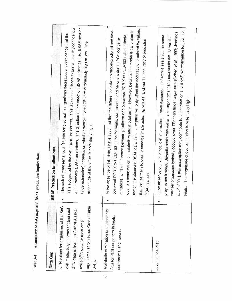
Tab
le 3
-4
A s
umm
ary
of d
ata
gaps
and
BSA
F p
redi
ctio
n im
plic
atio
ns
615N
valu
es fo
r or
gani
sms
of t
he S
oG
diet
mat
rix (e
.g.,
corm
oran
t and
sea
l
61
5~
da
ta is
from
the
Gul
f of
Ala
ska,
whi
le 6
I5N
data
for
mos
t oth
er
orga
nism
s is
from
Fal
se C
reek
(T
able
6-4
)).
Met
abol
ic e
limin
atio
n ra
te c
onst
ants
(kM) fo
r P
CB
con
gene
rs in
sea
ls,
corm
oran
ts, a
nd h
eron
s.
Juve
nile
sea
l die
t
BS
AF
Pre
dict
ion
Impl
icat
ions
-
The
lack
of
repr
esen
tativ
e 61
5N d
ata
for
diet
mat
rix o
rgan
ism
s de
crea
ses
my
conf
iden
ce th
at th
e
TP
s su
gges
ted
by th
e di
et m
atrix
are
cor
rect
. T
his
lack
of c
onfid
ence
in tu
rn a
ffect
s m
y co
nfid
ence
in th
e m
odel
's B
SA
F p
redi
ctio
ns.
The
dire
ctio
n of
the
effe
ct o
n B
SA
F e
stim
ates
(i.e
., B
SA
F o
ver
or
unde
rest
imat
ion)
dep
ends
on
whe
ther
mat
rix-im
plie
d T
Ps
are
erro
neou
sly
high
or
low
. T
he
mag
nitu
de o
f the
effe
ct is
pot
entia
lly h
igh.
In th
e ab
senc
e of
thi
s da
ta, I h
ave
assu
med
that
the
diffe
renc
e be
twee
n m
odel
-pre
dict
ed an
d fie
ld-
obse
rved
PC
B-X
to P
CB
-1 53
rat
ios
for
seal
s, c
orm
oran
ts, a
nd h
eron
s is
due
to P
CB
con
gene
r
met
abol
ism
. T
he d
iffer
ence
bet
wee
n pr
edic
ted
and
obse
rved
PC
B-X
to P
CB
-153
ratio
s is
like
ly
due
to a
com
bina
tion
of m
etab
olis
m a
nd m
odel
err
or.
How
ever
, bec
ause
the
mod
el is
cal
ibra
ted
to
mat
ch th
e ob
serv
ed B
SA
F d
ata,
this
ass
umpt
ion
will
onl
y af
fect
the
accu
racy
of p
redi
cted
kM
valu
es
(i.e.
, cau
se th
em to
ove
r or
und
eres
timat
e ac
tual
kM
valu
es)
and
not t
he a
ccur
acy
of p
redi
cted
BS
AF
val
ues.
In th
e ab
senc
e of
juve
nile
sea
l die
t inf
orm
atio
n, I h
ave
assu
med
that
juve
nile
sea
ls e
at th
e sa
me
prey
as
adul
t sea
ls.
Juve
nile
sea
ls m
ay e
at s
mal
ler o
rgan
ism
s th
an th
ose
adul
ts e
at.
Giv
en th
at
smal
ler o
rgan
ism
s ty
pica
lly o
ccup
y lo
wer
TP
s th
an la
rger
org
anis
ms
[Coh
en e
t a/.
, 199
3; J
enni
ngs
eta
!., 2
0011
, thi
s as
sum
ptio
n m
ay c
ontr
ibut
e to
con
cent
ratio
n an
d B
SA
F o
vere
stim
atio
n fo
r juv
enile
seal
s. T
he m
agni
tude
of o
vere
stim
atio
n is
pot
entia
lly h
igh.
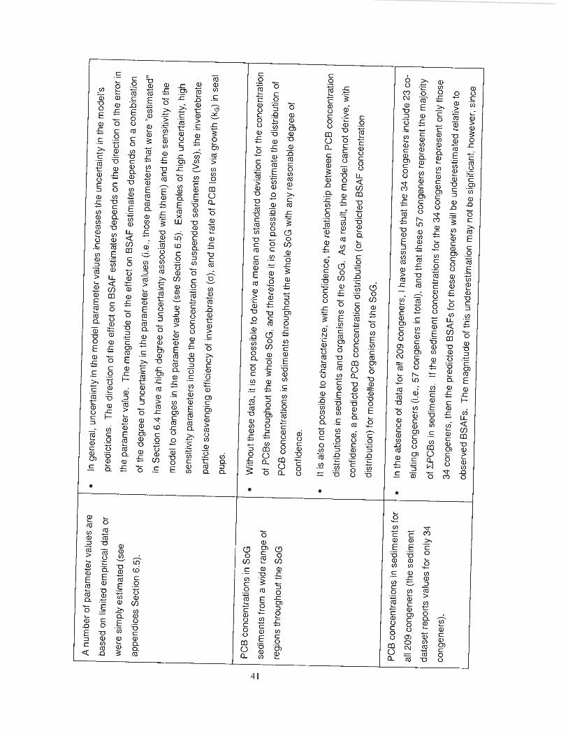
4 nu
mbe
r of
para
met
er v
alue
s ar
e
oase
d on
lim
ited
empi
rical
dat
a or
wer
e si
mpl
y es
timat
ed (s
ee
appe
ndic
es S
ectio
n 6.
5).
PC
B c
once
ntra
tions
in S
oG
sedi
men
ts fr
om a
wid
e ra
nge
of
regi
ons
thro
ugho
ut th
e S
oG
PC
B c
once
ntra
tions
in s
edim
ents
for
all 2
09 c
onge
ners
(the
sed
imen
t
data
set r
epor
ts v
alue
s fo
r on
ly 3
4
cong
ener
s).
In g
ener
al, u
ncer
tain
ty in
the
mod
el p
aram
eter
val
ues
incr
ease
s th
e un
cert
aint
y in
the
mod
el's
pred
ictio
ns.
The
dire
ctio
n of
the
effe
ct o
n B
SA
F e
stim
ates
dep
ends
on
the
dire
ctio
n of
the
err
or in
the
para
met
er v
alue
. T
he m
agni
tude
of
the
effe
ct o
n B
SA
F e
stim
ates
dep
ends
on
a co
mbi
natio
n
of t
he d
egre
e of
unc
erta
inty
in th
e pa
ram
eter
val
ues
(i.e.
, tho
se p
aram
eter
s th
at w
ere
"est
imat
ed"
in S
ectio
n 6.
4 ha
ve a
hig
h de
gree
of
unce
rtai
nty
asso
ciat
ed w
ith th
em)
and
the
sens
itivi
ty o
f the
mod
el to
cha
nges
in th
e pa
ram
eter
val
ue (
see
Sec
tion
6.5)
. E
xam
ples
of
high
unc
erta
inty
, hig
h
sens
itivi
ty p
aram
eter
s in
clud
e th
e co
ncen
trat
ion
of s
uspe
nded
sed
imen
ts (V
ss),
the
inve
rteb
rate
part
icle
sca
veng
ing
effic
ienc
y of
inv
erte
brat
es (o
), a
nd th
e ra
te o
f P
CB
loss
via
gro
wth
(kG
) in
seal
PUPS
.
With
out t
hese
dat
a, it
is n
ot p
ossi
ble
to d
eriv
e a
mea
n an
d st
anda
rd d
evia
tion
for
the
conc
entr
atio
n
of P
CB
s th
roug
hout
the
who
le S
oG, a
nd th
eref
ore
it is
not
pos
sibl
e to
est
imat
e th
e di
strib
utio
n of
PC
B c
once
ntra
tions
in s
edim
ents
thro
ugho
ut th
e w
hole
SoG
with
any
rea
sona
ble
degr
ee o
f
conf
iden
ce.
It is
als
o no
t pos
sibl
e to
cha
ract
eriz
e, w
ith c
onfid
ence
, the
rel
atio
nshi
p be
twee
n P
CB
con
cent
ratio
n
dist
ribut
ions
in s
edim
ents
and
org
anis
ms
of t
he S
oG.
As
a re
sult,
the
mod
el c
anno
t der
ive,
with
conf
iden
ce,
a pr
edic
ted
PC
B c
once
ntra
tion
dist
ribut
ion
(or
pred
icte
d B
SA
F c
once
ntra
tion
dist
ribut
ion)
for
mod
elle
d or
gani
sms
of t
he S
oG.
In th
e ab
senc
e of
dat
a fo
r al
l 209
con
gene
rs, I
hav
e as
sum
ed th
at th
e 34
con
gene
rs in
clud
e 23
co-
elut
ing
cong
ener
s (i.
e., 5
7 co
ngen
ers
in to
tal),
and
that
thes
e 57
con
gene
rs r
epre
sent
the
maj
ority
of C
PC
Bs
in s
edim
ents
. If
the
sedi
men
t con
cent
ratio
ns fo
r th
e 34
con
gene
rs re
pres
ent o
nly
thos
e
34 c
onge
ners
, the
n th
e pr
edic
ted
BS
AF
s fo
r th
ese
cong
ener
s w
ill b
e un
dere
stim
ated
rela
tive
to
obse
rved
BS
AF
s. T
he m
agni
tude
of t
his
unde
rest
imat
ion
may
not
be
sig
nific
ant,
how
ever
, sin
ce

PC
B c
once
ntra
tions
in S
oG h
errin
g
from
reg
ions
oth
er th
an S
emia
hmoo
.
I
PC
B c
once
ntra
tions
in S
oG s
alm
on
(dat
a us
ed in
the
mod
el is
from
salm
on b
ough
t fro
m V
anco
uver
supe
rmar
kets
).
the
34 li
sted
con
gene
rs a
re th
e do
min
ant c
onge
ners
in th
e co
-elu
ting
grou
ps.
PC
B c
once
ntra
tions
sed
imen
t,
herr
ing,
and
sal
mon
from
logi
cally
sequ
entia
l dat
es
It is
not
cle
ar to
wha
t ext
ent P
CB
con
cent
ratio
ns in
her
ring
from
Sem
iahm
oo re
pres
ent P
CB
conc
entra
tions
in h
errin
g th
roug
hout
the
SoG
. O
ne re
cent
repo
rt [W
est e
t al.,
200
61 in
dica
tes
that
herr
ing
from
Sem
iahm
oo h
ave
EP
CB
bod
y bu
rden
s th
at a
re tw
ice
as h
igh
as h
errin
g fro
m th
e
mor
e re
mot
e D
enm
an Is
land
in th
e no
rthe
rn S
oG (
i.e.,
34 v
s. 1
8 ng
/g-w
w,
resp
ectiv
ely)
. T
his
sugg
ests
that
the
herr
ing
conc
entr
atio
ns u
sed
in th
e m
odel
may
repr
esen
t the
upp
er e
nd o
f the
herr
ing'
s P
CB
con
cent
ratio
n ra
nge
thro
ugho
ut th
e S
oG.
If so
, I w
ould
exp
ect t
his
data
gap
to
cont
ribut
e to
the
over
estim
atio
n of
BS
AF
s fo
r al
l her
ring
pred
ator
s. T
he d
egre
e of
this
over
estim
atio
n m
ay b
e hi
gh fo
r or
gani
sms
that
eat
sig
nific
ant q
uant
ities
of
herr
ing
(e.g
., 25
% o
f the
seal
die
t is
her
ring)
.
Sto
re b
ough
t sal
mon
may
or
may
not
hav
e P
CB
con
cent
ratio
ns e
quiv
alen
t to
PC
B c
once
ntra
tions
in s
alm
on m
igra
ting
thro
ugh
the
SoG
's.
Usi
ng P
CB
con
cent
ratio
ns fr
om s
tore
bou
ght s
alm
on a
s
mod
el in
put m
ay c
ontr
ibut
e to
the
over
or
unde
rest
imat
ion
of B
SA
Fs fo
r al
l sal
mon
pre
dato
rs.
How
ever
, sin
ce s
alm
on c
ompr
ise
only
a s
mal
l por
tion
of t
he d
iets
of S
oG to
p pr
edat
ors
of in
tere
st
(Tab
le 3
-I),
the
degr
ee o
f B
SA
F un
der
or o
vere
stim
atio
n is
not
exp
ecte
d to
be
sign
ifica
nt.
Pre
dato
rs in
the
mod
el c
onsu
me
herr
ing
from
200
3, s
alm
on fr
om 2
004,
and
hak
e an
d ot
her
prey
item
s fro
m s
ome
earli
er d
ate
(i.e.
, 19
97 -t
he
sed
imen
t sam
plin
g ye
ar - p
lus
the
time
it ta
ke fo
r
PC
Bs
to m
ove
from
sed
imen
ts u
p th
roug
h th
e fo
od w
eb).
If P
CB
con
cent
ratio
ns fr
om t
he th
ree
inpu
t med
ia re
mai
ned
rela
tivel
y co
nsta
nt fr
om 1
997
to 2
004,
then
the
tem
pora
l diff
eren
ce b
etw
een
sam
plin
g da
tes
of e
ach
does
not
mat
ter.
If t
he r
atio
of
PC
B c
once
ntra
tions
in h
errin
g an
dlor
salm
on to
sed
imen
t inc
reas
ed o
ver t
his
time
perio
d, th
en th
is d
ata
gap
will
con
trib
ute
to
over
estim
atio
n of
the
pre
dict
ed B
SA
F, a
nd v
ice
vers
a.
3.2 Model Performance Analysis
I assessed the model's performance by (i) comparing, graphically, the model predicted
BSAFs to empirically derived BSAFs on a congener-specific basis, (ii) calculating the
model bias (MB) for these observed vs. predicted BSAF graphs, and (iii) comparing these
MB values graphically to congener log-Kow values. The methods for each of these are
described below.
3.2.1 Comparison of Predicted and Observed BSAFs
I derived predicted congener-specific BSAFs by dividing predicted organism
concentrations by observed sediment concentrations (i.e. those used to run the model). I
derived observed congener-specific BSAFs by dividing observed organism
concentrations by observed sediment concentrations (i.e., the same sediment
concentrations used to derive predicted BSAFs). I then plotted the predicted and
observed BSAFs on the same graph for visual comparison on both a congener-specific
and CPCB basis. The CPCB-BSAF values were calculated as follows:
BSAFxpcn= (C Ca) / (C C S ~ )
Where CB (ndg-ww) is the concentration of congener i in the organism, and Cs (nglg-
dw) is the concentration of congener i in the sediment. Note that the CPCB analysis was
performed only for top predators because these organisms have the most reliable
performance analysis datasets and because these organisms are of most concern from a
risk management standpoint.
3.2.2 MB Calculations and Analysis
I estimated the MB using the following equation:

Where BSAFp (unitless) is the predicted BSAF for congener i, BSAFo (unitless) is the
observed BSAF for congener i, and n is the number of congeners. The MB is an
indication of the under- or over-prediction by the model. For instance, if the model-
predicted BSAF for congener 153 in seal pups is 200, and the observed BSAF for
congener 153 in seal pups is 100, then the MB for congener 153 in seal pups is 2.0.
In addition, I plotted the ratio of BSAFp to BSAFo vs. log-Kow for each congener in seal
mothers, seal pups, cormorant eggs, and heron eggs. The BSAFp/BSAFo should be
independent of log-Kow; a correlation between BSAFp/BSAFo and log-Kow is indicative
of systematic bias in the model.
3.2.3 Data Gaps and Model Performance Analysis Implications
The key data gaps of concern for model perfomlance analysis are presented below (Table
3-5).
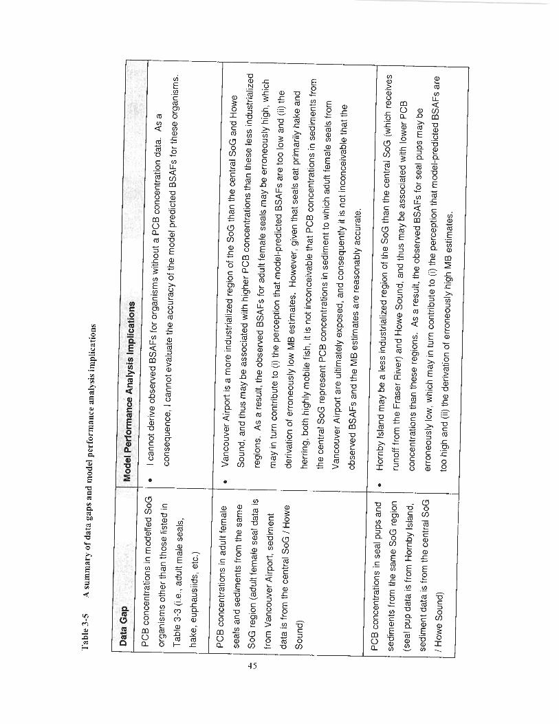
Tab
le 3
-5
A s
umm
ary
of d
ata
gaps
and
mod
el p
erfo
rman
ce a
naly
sis i
mpl
icat
ions
Dat
a G
ap
PC
B c
once
ntra
tions
in m
odel
led
SoG
orga
nism
s ot
her t
han
thos
e lis
ted
in
Tab
le 3
-3 (i
.e.,
adul
t mal
e se
als,
hake
, eup
haus
iids,
etc
.)
PC
B c
once
ntra
tions
in a
dult
fem
ale
seal
s an
d se
dim
ents
from
the
sam
e
SoG
reg
ion
(adu
lt fe
mal
e se
al d
ata
is
from
Van
couv
er A
irpor
t, se
dim
ent
data
is fr
om th
e ce
ntra
l SoG
/ H
owe
Sou
nd)
PC
B c
once
ntra
tions
in s
eal p
ups
and
sedi
men
ts fr
om th
e sa
me
SoG
reg
ion
(sea
l pup
dat
a is
from
Hor
nby
Isla
nd,
sedi
men
t dat
a is
from
the
cent
ral S
oG
/ H
owe
Sou
nd)
Mod
el ~
erfo
rrn
anc6
An
alys
is Im
plic
atio
ns
I can
not d
eriv
e ob
serv
ed B
SA
Fs
for
orga
nism
s w
ithou
t a P
CB
con
cent
ratio
n da
ta.
As
a
cons
eque
nce,
I ca
nnot
eva
luat
e th
e ac
cura
cy o
f the
mod
el p
redi
cted
BS
AF
s fo
r the
se o
rgan
ism
s.
Van
couv
er A
irpor
t is
a m
ore
indu
stria
lized
regi
on o
f the
SoG
than
the
cent
ral S
oG a
nd H
owe
Sou
nd, a
nd th
us m
ay b
e as
soci
ated
with
hig
her P
CB
con
cent
ratio
ns th
an th
ese
less
indu
stria
lized
regi
ons.
As
a re
sult,
the
obse
rved
BS
AF
s fo
r ad
ult f
emal
e se
als
may
be
erro
neou
sly
high
, whi
ch
may
in tu
rn c
ontri
bute
to (
i) th
e pe
rcep
tion
that
mod
el-p
redi
cted
BS
AFs
are
too
low
and
(ii)
the
deriv
atio
n of
err
oneo
usly
low
MB
est
imat
es.
How
ever
, giv
en th
at s
eals
eat
prim
arily
hak
e an
d
herr
ing,
bot
h hi
ghly
mob
ile fi
sh, i
t is
not i
ncon
ceiv
able
that
PC
B c
once
ntra
tions
in s
edim
ents
from
the
cent
ral S
oG r
epre
sent
PC
B c
once
ntra
tions
in s
edim
ent t
o w
hich
adu
lt fe
mal
e se
als
from
Van
couv
er A
irpor
t are
ulti
mat
ely
expo
sed,
and
con
sequ
ently
it is
not
inco
ncei
vabl
e th
at th
e
obse
rved
BS
AFs
and
the
MB
est
imat
es a
re r
easo
nabl
y ac
cura
te.
Hor
nby
Isla
nd m
ay b
e a
less
indu
stria
lized
regi
on o
f the
SoG
than
the
cent
ral S
oG (
whi
ch re
ceiv
es
runo
ff fro
m th
e F
rase
r Riv
er) a
nd H
owe
Sou
nd, a
nd th
us m
ay b
e as
soci
ated
with
low
er P
CB
conc
entra
tions
than
thes
e re
gion
s. A
s a
resu
lt, th
e ob
serv
ed B
SA
Fs
for
seal
pup
s m
ay b
e
erro
neou
sly
low
, whi
ch m
ay in
turn
con
trib
ute
to (
i) th
e pe
rcep
tion
that
mod
el-p
redi
cted
BS
AF
s ar
e
too
high
and
(ii)
the
deriv
atio
n of
err
oneo
usly
hig
h M
B e
stim
ates
.
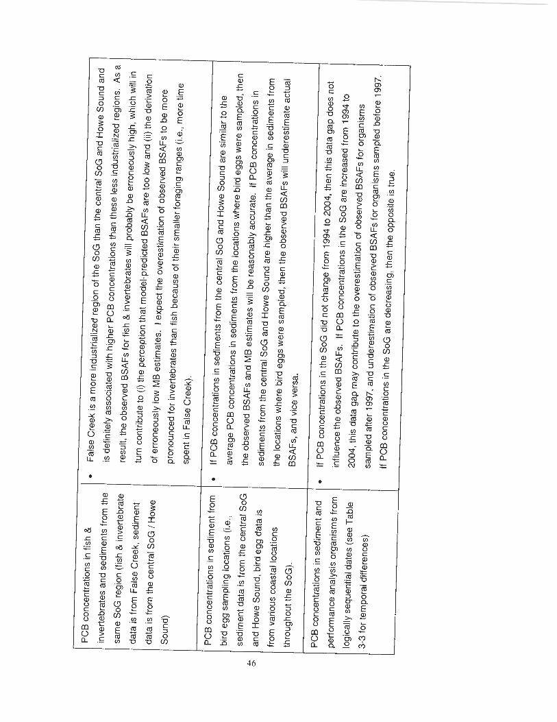
PC
B c
once
ntra
tions
in fi
sh &
inve
rteb
rate
s an
d se
dim
ents
from
the
sam
e S
oG re
gion
(fis
h &
inve
rteb
rate
data
is fr
om F
alse
Cre
ek, s
edim
ent
data
is fr
om th
e ce
ntra
l SoG
/ H
owe
Sou
nd)
PC
B c
once
ntra
tions
in s
edim
ent f
rom
bird
egg
sam
plin
g lo
catio
ns (i
.e.,
sedi
men
t dat
a is
from
the
cent
ral S
oG
and
How
e S
ound
, bird
egg
dat
a is
from
var
ious
coa
stal
loca
tions
thro
ugho
ut th
e S
oG).
PC
B c
once
ntra
tions
in s
edim
ent a
nd
perf
orm
ance
ana
lysi
s or
gani
sms
from
logi
cally
seq
uent
ial d
ates
(see
Tab
le
3-3
for
tem
pora
l diff
eren
ces)
Fal
se C
reek
is a
mor
e in
dust
rializ
ed re
gion
of t
he S
oG th
an th
e ce
ntra
l SoG
and
How
e S
ound
and
is d
efin
itely
ass
ocia
ted
with
hig
her
PC
B c
once
ntra
tions
than
thes
e le
ss in
dust
rializ
ed re
gion
s. A
s a
resu
lt, th
e ob
serv
ed B
SA
Fs fo
r fis
h &
inve
rteb
rate
s w
ill p
roba
bly
be e
rron
eous
ly h
igh,
whi
ch w
ill in
turn
con
trib
ute
to (
i) th
e pe
rcep
tion
that
mod
el-p
redi
cted
BS
AF
s ar
e to
o lo
w a
nd (
ii) th
e de
rivat
ion
of e
rron
eous
ly lo
w M
B e
stim
ates
. I e
xpec
t the
ove
rest
imat
ion
of o
bser
ved
BS
AF
s to
be
mor
e
pron
ounc
ed fo
r in
vert
ebra
tes
than
fish
bec
ause
of t
heir
smal
ler f
orag
ing
rang
es (i
.e.,
mor
e tim
e
spen
t in
Fal
se C
reek
).
- -
--
If P
CB
con
cent
ratio
ns in
sed
imen
ts fr
om th
e ce
ntra
l SoG
and
How
e S
ound
are
sim
ilar t
o th
e
aver
age
PC
B c
once
ntra
tions
in s
edim
ents
from
the
loca
tions
whe
re b
ird e
ggs
wer
e sa
mpl
ed, t
hen
the
obse
rved
BS
AFs
and
MB
est
imat
es w
ill b
e re
ason
ably
acc
urat
e.
If P
CB
con
cent
ratio
ns in
sedi
men
ts fr
om th
e ce
ntra
l SoG
and
How
e S
ound
are
hig
her t
han
the
aver
age
in s
edim
ents
from
the
loca
tions
whe
re b
ird e
ggs
wer
e sa
mpl
ed, t
hen
the
obse
rved
BS
AFs
will
und
eres
timat
e ac
tual
BS
AF
s, a
nd v
ice
vers
a. -
If P
CB
con
cent
ratio
ns in
the
SoG
did
not
cha
nge
from
199
4 to
200
4, th
en th
is d
ata
gap
does
not
influ
ence
the
obse
rved
BS
AF
s. I
f PC
B c
once
ntra
tions
in th
e S
oG a
re in
crea
sed
from
199
4 to
2004
, thi
s da
ta g
ap m
ay c
ontr
ibut
e to
the
over
estim
atio
n of
obs
erve
d B
SA
Fs fo
r or
gani
sms
sam
pled
afte
r 19
97, a
nd u
nder
estim
atio
n of
obs
erve
d B
SA
Fs fo
r or
gani
sms
sam
pled
bef
ore
1997
.
If P
CB
con
cent
ratio
ns in
the
SoG
are
dec
reas
ing,
then
the
oppo
site
is tr
ue.

3.3 Model Application
3.3.1 Overvicw
Once the model performance analysis was satisfactorily completed, I used the model-
predicted and empirical BSAFs to facilitate an ecological risk assessment (ERA) for seals
and cormorants of the SoG, evaluation of the current SQG for CPCBs, recommendation
of a new SQG for CPCBs, and proposal of SoG-specific SQTs for CPCBs. The methods
for each of these applications are described below.
3.3.2 Ecological Risk Assessment for Top Predators
3.3.2.1 Overview
ERA is a process for evaluating the likelihood that adverse ecological effects are
occurring or may occur as a result of exposure to one or more stressors [US EPA, 19921.
I conducted an ERA to evaluate the potential risks posed by PCB exposure to adult
female seal, seal pup, and cormorant egg populations in the SoG. The ERA for each
receptor group is based on a single line of evidence: comparison of predicted and
observed CPCB body burdens with CPCB concentrations suspected to cause adverse
effects. The incorporation of additional lines of evidence (e.g., field observations,
laboratory tests, etc.) is beyond the scope of this project. I derived the CPCB body
burdens and CPCB effects concentrations for the exposure and effects comparison as
described below. Note that the ERA was limited to seal and cormorant receptors because
these were the only top predators for which I could obtain effects data.
3.3.2.2 ERA for Seals
CPCB Effects Estimation
I obtained CPCB effects data for seals from the literature. Kannan et a/., 2000 reviewed a
study reported in Boon et al., 1987 and Brouwer et al., 1989 where one group of captive
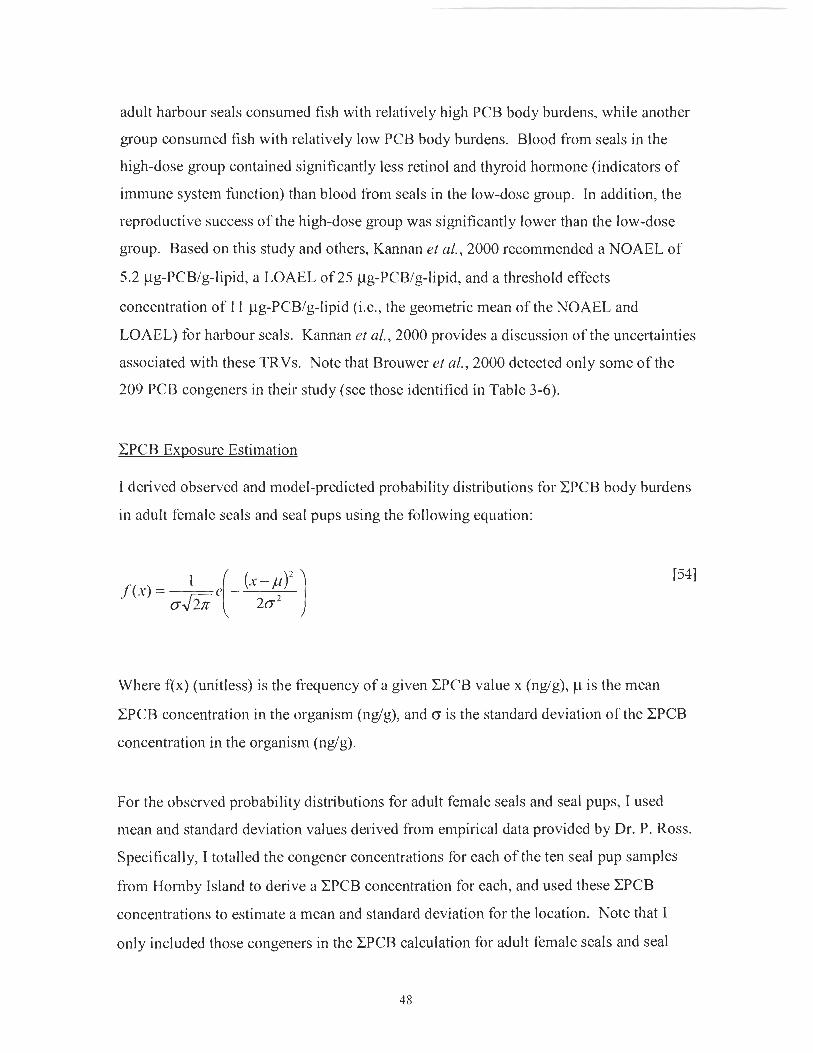
adult harbour seals consumed fish with relatively high PCB body burdens, while another
group consumed fish with relatively low PCB body burdens. Blood from seals in the
high-dose group contained significantly less retinol and thyroid hormone (indicators of
immune system .hnction) than blood from seals in the low-dose group. In addition, the
reproductive success of the high-dose group was significantly lower than the low-dose
group. Based on this study and others, Kannan et nl., 2000 recommended a NOAEL of
5.2 yg-PCBIg-lipid, a LOAEL of 25 yg-PCBIg-lipid, and a threshold effects
concentration of 11 pg-PCBIg-lipid (i.e., the geometric mean of the NOAEL and
LOAEL) for harbour seals. Kannan et al., 2000 provides a discussion of the uncertainties
associated with these TRVs. Note that Brouwer et al., 2000 detected only some of the
209 PCB congeners in their study (see those identified in Table 3-6).
CPCB Exposure Estimation
1 derived observed and model-predicted probability distributions for CPCB body burdens
in adult female seals and seal pups using the following equation:
Where f(x) (unitless) is the frequency of a given CPCB value x (nglg), p is the mean
CPCB concentration in the organism (nglg), and o is the standard deviation of the CPCB
concentration in the organism (nglg).
For the observed probability distributions for adult female seals and seal pups, I used
mean and standard deviation values derived from empirical data provided by Dr. P. Ross.
Specifically, I totalled the congener concentrations for each of the ten seal pup samples
from Hornby Island to derive a CPCB concentration for each, and used these CPCB
concentrations to estimate a mean and standard deviation for the location. Note that I
only included those congeners in the CPCB calculation for adult female seals and seal

pups that matched, as much as possible, the congeners used to derive the TRV (see Table
3-6 for details).
For the model-predicted probability distributions for adult female seals and seal pups, I
used as the mean the CPCB concentrations predicted by the model (i.e., those estimated
from PCB concentrations in central-SoG sediments, Semiahmoo herring, and
supennarket salmon). I used as a standard deviation the observed standard deviation for
CPCB concentrations in cormorant eggs (data provided by Dr. J. Elliott). I used the
observed cormorant egg standard deviation to represent the variability in seals because,
unlike the observed seal standard deviations, the observed cormorant variability
represents a relatively wide spatial range in the SoG (Figure 3-2). Furthermore,
coimorants occupy a similar TP as seals, like seals they eat only marine fishes, and the
observed SD for CPCB concentrations in cormorants is not unrealistic (for instance, the
SDs of the log-CPCB values for adult female seals from Vancouver Airport and the
connorant eggs from throughout the SoG are 0.18 and 0.26 ng/g-lipid, respectively).
Note that I only included those congeners in the CPCB calculation for adult female seals
and seal pups that matched, as closely as possible, the congeners used to derive the TRV
(see Table 3-6 for details).

Table 3-6 PCB congeners used to calculate the seal TRVs and the CPCB concentration distributions for model-predicted seals, observed adult female seals, and observed seal pups used in the ERA
Source --
Seal TRVs CPCB
Model-Predicted
3.3.2.3 ERA for Cormorants
CPCB Effects Estimation
oncentration Di Observed Adul
Seal 18/30 20128 26129
37 40/41/71 44/47/65
49/69 52
59/62/75 60
61 /70/74/76 66 78
83199 84
87/97/108/119112! 90/101/113
92 939519811001102
105 llOlIl5
118 1 2811 66
12911 3811 6011 63 135/151/154
I36 137
1391140 141
153168 156/157
170 172 177
180/193 183/185
I87 194 1 95
197/200 201 209
Dr. P. Ross
ibution Observed Seal Pup
18 38 26
37/59/42
209 Dr. P. Ross
I obtained CPCB effects data for cormorant eggs from the literature. In their ERA for
cormorant eggs in the San Francisco Bay, Gobas & Arnot, 2005 used a LOAEL of 5.0

pg/g-ww and cited Hoffman ct nl., 1996 as the source of this TRV. Gobas & Amot noted
that cormorant exposure to CPCB concentrations in this range is associated with
embryonic mortality, beak deformities, and club foot in the field [Gobas & Amot, 20051.
I was unable to obtain a copy of the Hoffman et nl., 1996 publication to confirm this
LOAEL. I was also unable to locate a published effects threshold or NOAEL for
cormorant egg exposure to CPCBs. I instead estimated a NOAEL by multiplying the
LOAEL by 0.1 ; apparently this approach was used by Hoffman et al., 1996 as well [Dr.
F. Gobas, personal cornnzunicntion]. I was also unable to determine which PCB
congeners were used to derive the CPCB concentration for the cormorant egg LOAEL.
CPCB Exposure Estimation
I derived observed and model-predicted probability distributions for CPCB body burdens
in cormorant eggs using equation 54. For the observed distribution, I used a mean and
standard deviation derived from empirical data piovided by Dr. J. Elliott. For the
predicted distribution, I used the mean value predicted by the model and the standard
deviation value derived from empirical data provided by Dr. J. Elliott. All congeners
were included in the CPCB estimation for the predicted and observed distributions.
3.3.3 Sediment Quality Guideline Evaluation and Recommendation
3.3.3.1 SQG Evaluation
I used two approaches to evaluate the level of protection offered by the current SQG for
CPCBs. First, I "forward calculated" the CPCB concentration in adult female seals, seal
pups, and cormorant eggs fkom the current SQG for CPCBs using the following equation:
Where CB-sQG (ng/g-ww) is the point estimate (i.e., not a distribution) CPCB
concentration associated with the current SQG (ng/g-dw) and BSAF (glg) is the predicted
BSAF for the organism. I then compared, graphically, the C B - S ~ G for each organism to
their respective TRVs and to their respective observed and predicted CPCB concentration
distributions (derived as described in Section 3.3.2).
Second, 1 again "forward calculated" the CPCB concentration in adult female seals and
cormorant eggs (but not seal pups) using Equation 55. This time, however, I multiplied
the SQG by both the observed and predicted BSAF for each organism, and, using the
resulting C B q G as a geometric mean for the organisms, the observed cormorant egg SD
as the SD for the organisms, and Equation 54, I estimated a CPCB concentration
distribution for each. I then compared these CPCB distributions to the TRVs for these
organisms. In effect, this approach estimates the CPCB concentration distributions and
levels of protection expected in adult female seals and cormorant eggs if the geometric
mean CPCB concentration in sediments of the SoG were at the SQG.
3.3.3.2 SQG Recommendation
The SQG for CPCBs is intended to ensure that all organisms in BC are exposed to "safe
levels" of PCBs [MOE, 20061. The results of the SQG evaluation (Section 4.4.2.2,
below) indicate that this protection goal is not being met for top predators of the SoG. To
derive a SQG for CPCBs that results in safe levels of CPCBs in adult female seals, seal
pups, and cormorant eggs, I "backward calculated" a CPCB concentration in sediment
fkom a CPCB concentration in these organisms using the following equation:
SQGli = NOAEL / BSAFp [W
Where SQGR (ng/g-dw) is the recommended SQG associated with protection to the
NOAEL, NOAEL (nglg-ww) is the NOAEL for the organism, and BSAFp (dg) is the
model-predicted BSAF for the organism.
3.3.4 Sediment Quality Target Proposals
To derive proposed SQTs for CPCBs that meet various protection goals (e.g., 5% of seal
pups above the NOAEL, 5% of cormorant eggs above the LOAEL, etc.), I "backward
calculated" CPCB concentrations in sediment from various target concentration in
organisms using the following equation:
SQT = CKI. / BSAFP ~571
Where SQT (ndg-dw) is the SQT, CST (ndg-ww) is the concentration target for the
organism, and BSAFp (dg ) if the model-predicted BSAF for the organism.
3.3.5 Data Gaps and model Application Implications
The key data gaps of concern for model application phase of the project are presented
below (Table 3-7).
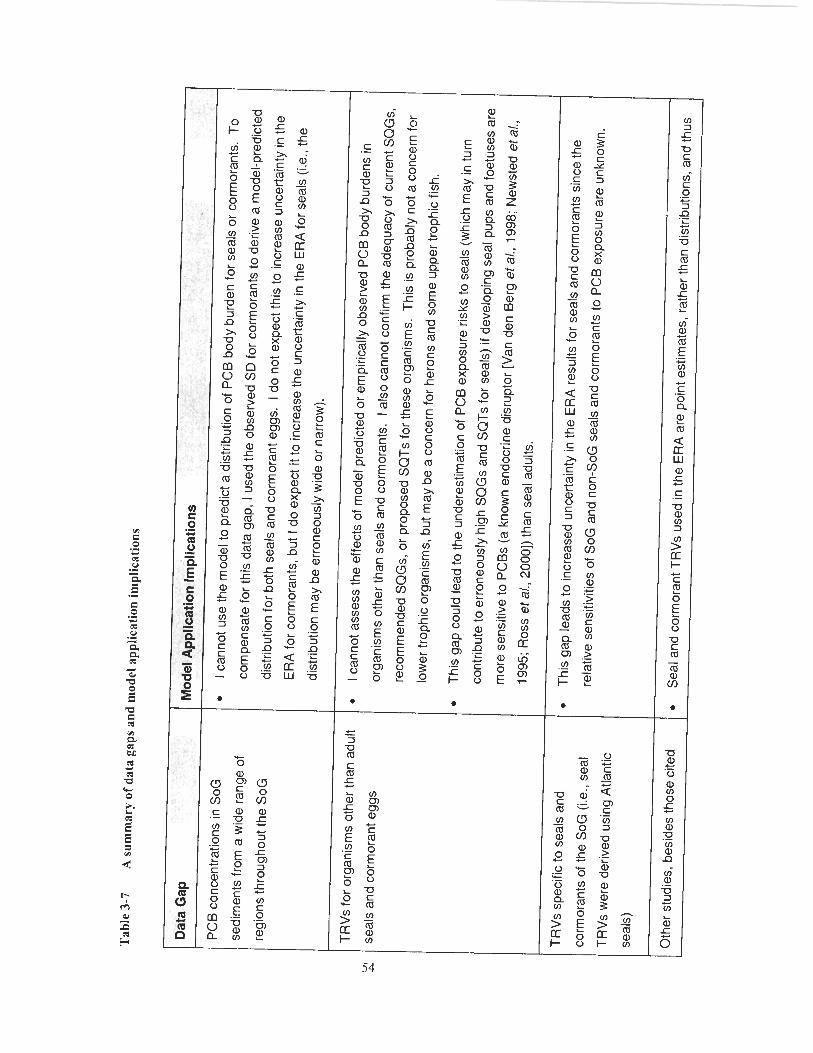
Tab
le 3
-7
A s
umm
ary
of d
ata
gaps
and
mod
el a
pplic
atio
n im
plic
atio
ns
Dat
a G
ap
PC
B c
once
ntra
tions
in S
oG
sedi
men
ts fr
on
a w
ide
rang
e of
regi
ons
thro
ugho
ut th
e S
oG
------ppppp
TR
Vs
for
orga
nism
s ot
her t
han
adul
t
seal
s an
d co
rmor
ant e
ggs
TR
Vs
spec
ific
to s
eals
and
corm
oran
ts o
f the
SoG
(i.e
., se
al
TR
Vs
wer
e de
rived
usi
ng A
tlant
ic
seal
s)
Oth
er s
tudi
es, b
esid
es th
ose
cite
d
Model
App
licat
ion
impl
icat
ions
I can
not u
se th
e m
odel
to p
redi
ct a
dis
trib
utio
n of
PC
B b
ody
burd
en fo
r sea
ls o
r co
rmor
ants
. T
o
com
pens
ate
for
this
dat
a ga
p, I u
sed
the
obse
rved
SD
for
corm
oran
ts to
der
ive
a m
odel
-pre
dict
ed
dist
ribut
ion
for
both
sea
ls a
nd c
orm
oran
t egg
s. I d
o no
t exp
ect t
his
to in
crea
se u
ncer
tain
ty in
the
ER
A fo
r co
rmor
ants
, but
I d
o ex
pect
it to
incr
ease
the
unce
rtai
nty
in th
e E
RA
for
seal
s (i.
e.,
the
dist
ribut
ion
may
be
erro
neou
sly
wid
e or
nar
row
).
I can
not a
sses
s th
e ef
fect
s of
mod
el p
redi
cted
or
empi
rical
ly o
bser
ved
PC
B b
ody
burd
ens
in
orga
nism
s ot
her t
han
seal
s an
d co
rmor
ants
. I a
lso
cann
ot c
onfir
m th
e ad
equa
cy o
f cu
rren
t SQ
Gs,
reco
mm
ende
d S
QG
s, o
r pr
opos
ed S
QTs
for
thes
e or
gani
sms.
Thi
s is
pro
babl
y no
t a c
once
rn fo
r
low
er tr
ophi
c or
gani
sms,
but
may
be
a co
ncer
n fo
r he
rons
and
som
e up
per t
roph
ic fi
sh.
Thi
s ga
p co
uld
lead
to th
e un
dere
stim
atio
n of
PC
B e
xpos
ure
risks
to s
eals
(w
hich
may
in tu
rn
cont
ribut
e to
err
oneo
usly
hig
h S
QG
s an
d S
QT
s fo
r se
als)
if d
evel
opin
g se
al p
ups
and
foet
uses
are
mor
e se
nsiti
ve to
PC
Bs
(a k
now
n en
docr
ine
disr
upto
r [V
an d
en B
erg
et a
/., 1
998;
New
sted
eta
/.,
1995
; Ros
s et
a/,
, 200
01) t
han
seal
adu
lts.
Thi
s ga
p le
ads
to in
crea
sed
unce
rtai
nty
in th
e E
RA
res
ults
for
seal
s an
d co
rmor
ants
sin
ce th
e
rela
tive
sens
itivi
ties
of S
oG a
nd n
on-S
oG s
eals
and
cor
mor
ants
to P
CB
exp
osur
e ar
e un
know
n.
Sea
l and
cor
mor
ant T
RV
s us
ed in
the
ER
A a
re p
oint
est
imat
es, r
athe
r tha
n di
strib
utio
ns, a
nd th
us
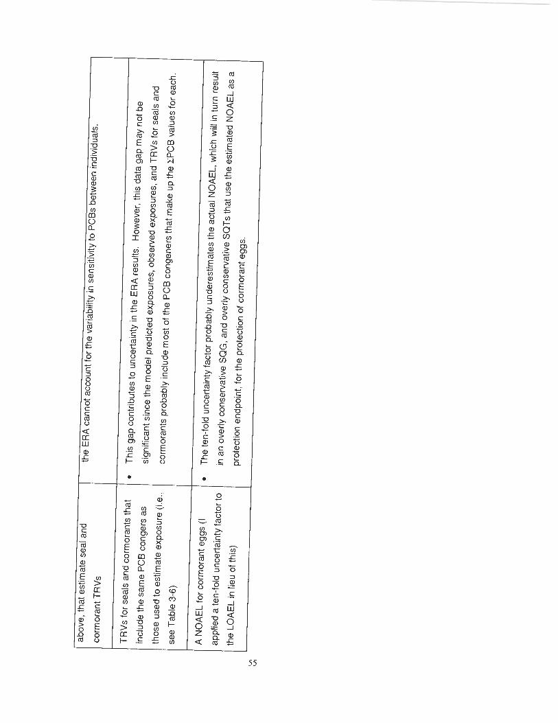
corm
oran
t TR
Vs
TR
Vs
for
seal
s an
d co
rmor
ants
that
incl
ude
the
sam
e P
CB
con
gers
as
thos
e us
ed to
est
imat
e ex
posu
re (i
.e.>
A N
OA
EL
for
corm
oran
t egg
s (I
appl
ied
a te
n-fo
ld u
ncer
tain
ty fa
ctor
to
the
LOA
EL
in li
eu o
f thi
s)
the
ER
A c
anno
t acc
ount
for t
he v
aria
bilit
y in
sen
sitiv
ity to
PC
Bs
betw
een
indi
vidu
als.
1
Thi
s ga
p co
ntrib
utes
to u
ncer
tain
ty in
the
ER
A re
sults
. H
owev
er, t
his
data
gap
may
not
be
sign
ifica
nt s
ince
the
mod
el p
redi
cted
exp
osur
es, o
bser
ved
expo
sure
s, a
nd T
RV
s fo
r se
als
and
corm
oran
is p
roba
bly
incl
ude
mos
t of
the
PC
B c
onge
ners
that
mak
e up
the
XPC
B v
alue
s fo
r ea
ch.
The
ten-
fold
unc
erta
inty
fact
or p
roba
bly
unde
rest
imat
es th
e ac
tual
NO
AE
L, w
hich
will
in tu
rn r
esul
t
in a
n ov
erly
con
serv
ativ
e S
QG
, and
ove
rly c
onse
rvat
ive
SQ
Ts
that
use
the
estim
ated
NO
AE
L as
a
prot
ectio
n en
dpoi
nt, f
or th
e pr
otec
tion
of c
orm
oran
t egg
s.

4 RESULTS & DISCUSSION
4.1 Accuracy of the Diet Matrix
Comparison with other studies
The model's diet matrix (Table 3- 1) as a whole did not conflict with the matrix by Pauly
& Christensen, 1995 (appendix Table 6-2) and in general had higher resolution. Fish
diets in the model did not differ from those in Froese & Pauly, 200 1. And there was good
agreement between the seal diet in the model and that reported in Olesiuk, 1993. For
instance, the proportion of hake, herring, salmonids, walleye pollock, and miscellaneous
demersals consumed by seals in the model fall within the range estimated by Olesiuk
(appendices Table 6-1). The only discrepancies between the seal diet in the model and
that in Olesiuk, 1993 are that small pelagic fish comprise a marginally larger proportion
of the seal's diet in the model, and dogfish are included as prey species in the model (0.1
% of the seal's diet) but were not reported as such in the Olesiuk paper. These minor
differences may simply be due to Olesiuk's inclusion of dogfish and some unidentified
pelagic fish in his unidentified/other category.
Trophic Position vs. F"N Ratios
Calculated TPs and literature derived 6I5N ratios and their references are presented in the
appendices (Table 6-3), while a plot of the relationship between TP and 615N is presented
below (Figure 4-1). It should be noted that 6ISN values for cormorants and adult seals
were taken from Gulf of Alaska organisms and are thus less than ideal for testing the
accuracy of the diet matrix. Also, FI5N values were not available for all species
represented by organism groups in the model (i.e., miscellaneous demersal fish, small
pelagic fish, predatory invertebrates, shellfish, and crabs); thus the range of 6 " ~ values
for these groups in Figure 4-1 may underestimate their true 6 " ~ variability.
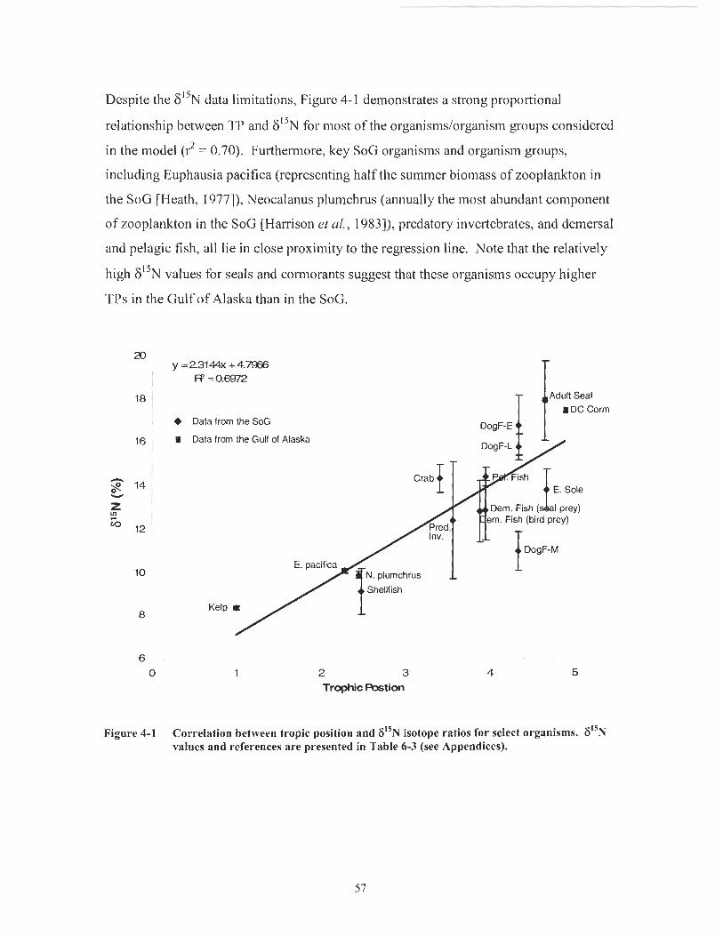
Despite the F"N data limitations, Figure 4-1 demonstrates a strong proportional
relationship between TP and F"N for most of the organisms/organism groups considered
in the model (r' = 0.70). Furthermore, key SoG organisms and organism groups,
including Euphausia pacifica (representing half the summer biomass of zooplankton in
the SoG [Heath, 1977]), Neocalanus plumchrus (annually the most abundant component
of zooplankton in the SoG [Harrison et a!., l983]), predatory invertebrates, and demersal
and pelagic fish, all lie in close proximity to the regression line. Note that the relatively
high F"N values for seals and cormorants suggest that these organisms occupy higher
TPs in the Gulf of Alaska than in the SoG.
+ Data from the SoG
Data from the Gulf of Alaska
Crab
Dem. Fish ( ( $ 1 prey) em. Fish (bird prey)
Adult Seal i DC Corm
Kelp
E. pacifica A N . plumchruo 1 / t Shellfish
2 3 Trophic Rostion
Figure 4-1 Correlation between tropic positiou and 6% isotope ratios for select organisms. 6% values and references are presented in Table 6-3 (see Appendices).

4.2 BSAF Predictions for CPCBs
Model-predicted BSAFs for CPCBs in modelled SoG organisms are presented in Figure
4-2. Log-BSAF values range from a low of -2.70 (or a BSAF of 0.002) g/g for
phytoplankton to a high of 2.7 1 (or a BSAF of 5 13) d g for seal pups. This represents an
increase in the BSAF of roughly 250,000 times (on a wet weight basis) from
phytoplankton to seal pups, and an increase in concentration of roughly 500 times from
sediment (dry weight) to seal pups (wet weight).
Note that BSAF values for organisms with similar diets fall within distinct ranges.
Specifically, herbivorous organisms, including Euphausia pacifica and grazing
invertebrates, occupy the log-BSAF range from -0.29 to 0.42 g/g (or BSAFs ranging
between 0.5 and 2.6 g/g). Invertebrate consumers, including pelagic fish (bird prey) and
demersal fish (seal prey), occupy the log-BSAF range from 0.69 to 1.1 3 g/g (or BSAFs
ranging between 4.9 and 13 dg). Piscivorous organisms, including dogfish and seal
pups, occupy the log-BSAF range from 1.55 to 2.71 g/g (or BSAFs ranging between 35
and 5 13). This result is consistent with previous food web studies [Gobas & Arnot, 2005;
Gobas et al., 1998; Morrison et al., 1997; Stevenson, 2003; Mackintosh et al., 20041 and
suggests that the model's mathematical structure is generally sound.

bg%SAF (g wet organisn / g dry sediment)
Figure 4-2 Predicted BSAFs for CPCB in all modelled organisms of the SoG
4.3 Model Performance Analysis
Evaluation of the model's performance allows one to gain a better understanding of the
model's strengths and weaknesses. This understanding is important because it allows
model users to maximize the model's potential as a decision-making tool and avoid
making poor decisions (or no decisions at all). To assess the model's performance, I (i)
compared, graphically, model-predicted BSAFs to observed BSAFs on a congener-
specific and CPCB basis, (ii) estimated the MB on a congener-specific and CPCB basis,
and (iii) compared the MB of individual congeners to their log-Kow values. The results
of these analyses are presented below.
4.3.1 Model Performance Analysis for PCB Congeners
Model-predicted and observed BSAFs are compared together, on a congener-specific
basis, in Figure 4-3 through to Figure 4- 12 (below). The corresponding MB results are
shown in Table 4- 1. Note that only organisms with a reasonable empirical dataset were
included in this analysis, and only the dominant of co-eluting congeners are listed on the
x-axis of the graphs.

Log-BSAF (g-wet-org / g-dry-sed)


d d o o L o O l o O s
(pas-hp-6 1 ~JO- I~M-~ ) j~sg-601

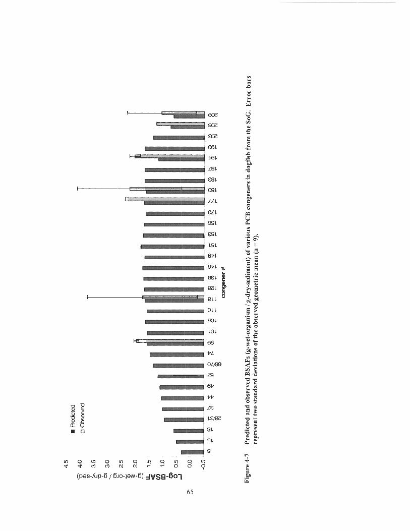
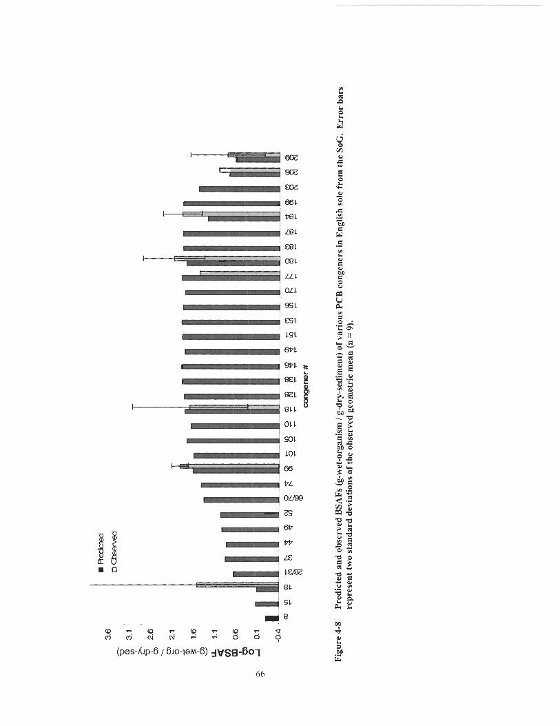


Log-BSAF (g-wet-.erg 1 g-dry-sed) f b g !=' A a 0 ul cn 0 h

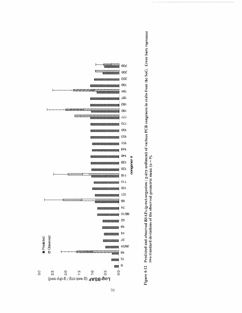
V1
081 L al
LLC 8 am a
OLC 0 0

Table 4-1 Individual and combined MB results (i.e., mean, lower 95%, and upper 95%) for select organisms of the SoG (i.e., those with a performance analysis dataset) on a congener- specific basis
Shellfish Crabs Predatory invertebrates Demersal fish (seal prey) bmersal fish (bird prey) Dogfish English sole Seal (adult female)
Seal (PUP) Cormorant egg Heron egg
All organisms
n = number of congeners on
Organism Lower 95% CI I Upper 95% CI
0.90 0.06 I 14.35
vhich the MB values are based. Co-eluting groups
I Model Bias
count as one congener.
n
Adult Female Seals
Mean
Comparison of observed and predicted BSAFs for adult female seals (Figure 4-3) and the
mean MB result for adult female seals (Table 4-1) reveal three key points about the
model's predictions. First, predicted BSAFs for adult female seals are in reasonable
agreement with the observed BSAFs - the majority of congener predicted BSAFs fall
within two standard deviations of observed geometric mean BSAFs. Only the BSAFs of
congener groups 8, 15,28/3 1,37,49,66/70, 1 10, and 149 (i.e., 8 of the 32 congener
groups) fall outside the observed range, all marginally above. Second, Figure 4-3 and the
corresponding mean MB of 1.47 (Table 4- 1) indicate that the model systematically over-
predicts, to a small extent, the BSAFs for adult female seals. Third, Figure 4-3 indicates
that the BSAFs of some of the most heavily chlorinated congeners (i.e., 194, 203, 206,
and 209) are under-predicted. This BSAF under-prediction could be the result of site

specific differences in the PCB congener pattern of sediments used as model input (i.e.,
those from central SoG) and sediments to which observed female seals (i.e., those used in
the model performance analysis) are exposed (i.e., sediments near Vancouver Airport).
Ross et al., 2004 found that more heavily chlorinated PCB congeners comprised a greater
proportion of CPCB concentrations in harbour seals from industrialized areas of the
Northeast Pacific Ocean than in harbour seals from remote areas of the Northeast Pacific
Ocean. The BSAF under-prediction for the most heavily chlorinated congeners could
also be due to model error. For instance, higher chlorinated PCBs may be selectively
retained by reproducing and nursing females to a greater extent than estimated by the
inodel.
Seal Pups
Figure 4-4, which compares observed and predicted BSAFs for seal pups, indicates that
agreement between inodel BSAF predictions and empirical data for seal pups is limited.
Only the BSAFs of congener groups 2813 1, 52,99, 105, 1 18, 138, 149, and 153 (i.e., 8 of
the 32 modelled congener groups) fall within two standard deviations of the observed
geometric means - the majority of congener predictions (i.e., 75%) fall outside the
observed range. Figure 4-4, and the corresponding mean MB of 2.10 for seal pups (Table
4- I), also indicate that the model systematically over-predicts the BSAFs for seal pups,
and does so to a greater degree than it does for adult female seals.
The systematic over-prediction of seal pup BSAFs could be due, in part, to a difference in
PCB concentrations in sediments from the central SoG (i.e., those used as input for the
model) and the northern SoG (i.e., those to which the empirical seal pups used to test the
model are probably exposed). For instance, if PCB concentrations in central SoG
sediments are higher than those in the northern SoG (I do not have the data to confirm
one way or the other), then model over-prediction for seal pups is not surprising. The
systematic over-prediction of seal pup BSAFs could also be due to model inaccuracies
(i.e., an inaccurate diet matrix, inaccurate kG and k~ values for seal pups, etc.).

Figure 4-4 also demonstrates, in contrast to the results for adult female seals (Figure 4-3),
a general trend of congener under-prediction to over-prediction fiom light to heavily
chlorinated congeners in seal pups. This trend could be the result of site specific
differences in the PCB congener pattern of sediments used as model input (i.e., those
from central SoG) and sediments to which observed seal pups (i.e., those used in the
model performance analysis) are exposed (i.e., sediments near Hornby Island). Ross et
al., 2004 found that more heavily chlorinated PCB congeners comprised a greater
proportion of CPCB concentrations in harbour seals from industrialized areas of the
Northeast Pacific Ocean than in harbour seals from remote areas of the Northeast Pacific
Ocean. The trend of BSAF under- to over-predictions of light to heavy chlorinated
congeners in seal pups could also be due to model error. For instance, higher chlorinated
PCBs may be selectively retained by reproducing and nursing females to a greater extent
than estimated by the model.
Bird E m s
Figure 4-5 and Figure 4-6 illustrate that predicted BSAFs for cormorant eggs and heron
eggs fall within two standard deviations of the observed geometric mean for all congener
groups except PCB- 15 1 in herons. Table 4- 1 shows a small systematic under-prediction
of the BSAF for cormorant eggs (mean MB = 0.63) and heron eggs (mean MB = 0.73).
Fish -
Figure 4-7 and Figure 4-8 indicate that, for English sole and dogfish, predicted BSAFs
for congeners 1 18, 180, and 209 fall within the two standard deviations of the observed
geometric means, while predicted BSAFs for congeners 99 and 194 fall outside the
observed range. BSAF predictions for PCB 18 also fall within two standard deviations of
the observed range for English sole, however the observed variability for this congener
was extremely large. Figure 4-9, which shows the BSAF comparison results for demersal
fish (seal prey), illustrates that predicted BSAFs for congeners 99, 1 18, 180, 194, and 209
fall within two standard deviations of the observed BSAF ranges, while the BSAF
prediction for congener 18 falls outside this range. Figure 4-10, which shows the BSAF
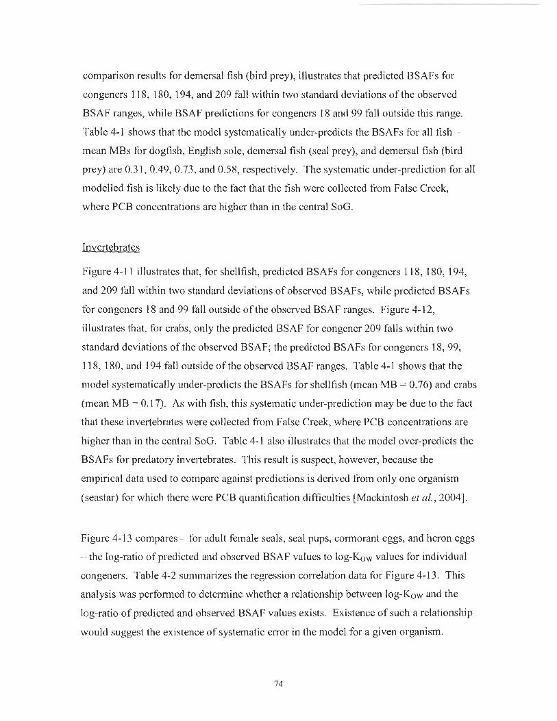
comparison results for demersal fish (bird prey), illustrates that predicted BSAFs for
congeners 1 18, 180, 194, and 209 fall within two standard deviations of the observed
BSAF ranges, while BSAF predictions for congeners 18 and 99 fall outside this range.
Table 4- 1 shows that the model systematically under-predicts the BSAFs for all fish -
mean MBs for dogfish, English sole, demersal fish (seal prey), and demersal fish (bird
prey) are 0.3 1, 0.49, 0.73, and 0.58, respectively. The systematic under-prediction for all
modelled fish is likely due to the fact that the fish were collected from False Creek,
where PCB concentrations are higher than in the central SoG.
Invertebrates
Figure 4- 1 1 illustrates that, for shellfish, predicted BSAFs for congeners 1 18, 180, 194,
and 209 fall within two standard deviations of observed BSAFs, while predicted BSAFs
for congeners 1 8 and 99 fall outside of the observed BSAF ranges. Figure 4- 12,
illustrates that, for crabs, only the predicted BSAF for congener 209 falls within two
standard deviations of the observed BSAF; the predicted BSAFs for congeners 18,99,
11 8, 180, and 194 fall outside of the observed BSAF ranges. Table 4-1 shows that the
model systematically under-predicts the BSAFs for shellfish (mean MB = 0.76) and crabs
(mean MB = 0.17). As with fish, this systematic under-prediction may be due to the fact
that these invertebrates were collected from False Creek, where PCB concentrations are
higher than in the central SoG. Table 4-1 also illustrates that the model over-predicts the
BSAFs for predatory invertebrates. This result is suspect, however, because the
empirical data used to compare against predictions is derived from only one organism
(seastar) for which there were PCB quantification difficulties [Mackintosh et al., 20041.
Figure 4-1 3 compares - for adult female seals, seal pups, cormorant eggs, and heron eggs
- the log-ratio of predicted and observed BSAF values to log-Kow values for individual
congeners. Table 4-2 summarizes the regression correlation data for Figure 4-1 3. This
analysis was performed to determine whether a relationship between log-Kow and the
log-ratio of predicted and observed BSAF values exists. Existence of such a relationship
would suggest the existence of systematic error in the model for a given organism.

Table 4-2 indicates that the slope of the regression lines are slightly negative for adult
female seals, cormorant eggs, and heron eggs (a = -0.16, -0.2 1, and -0.05, respectively).
The slope of the line for seal pups, on the other hand, is positive (a = 0.82). For adult
female seals, seal pups, and cormorant eggs, R2 values for the regression equations are
0.40, 0.37, and 0.35, respectively. This suggests that only 35-40% of the variation in the
log-ratio of predicted and observed BSAF for these organisms is explained by the log-
Kow. The p-values for these equations are well below 0.05 (Table 4-2), suggesting that
the results are statistically significant.
Together, the R2 and p-values for the regression equations for adult female seals, seal
pups, and cormorant eggs indicate a weak to moderate relationship between the log-ratio
of predicted and observed BSAF values and log-Kow for each congener assessed. This
result provides weak to moderate support for the existence of systematic error in the
model for these three top predators. For heron eggs, the R~ and p-values of 0.01 and 0.5,
respectively, suggest that no relationship exists between the log-ratio of predicted and
observed BSAF values and log-Kow for the congeners assessed, and thus no evidence
exists for the existence of systematic error in the model for this top predator.
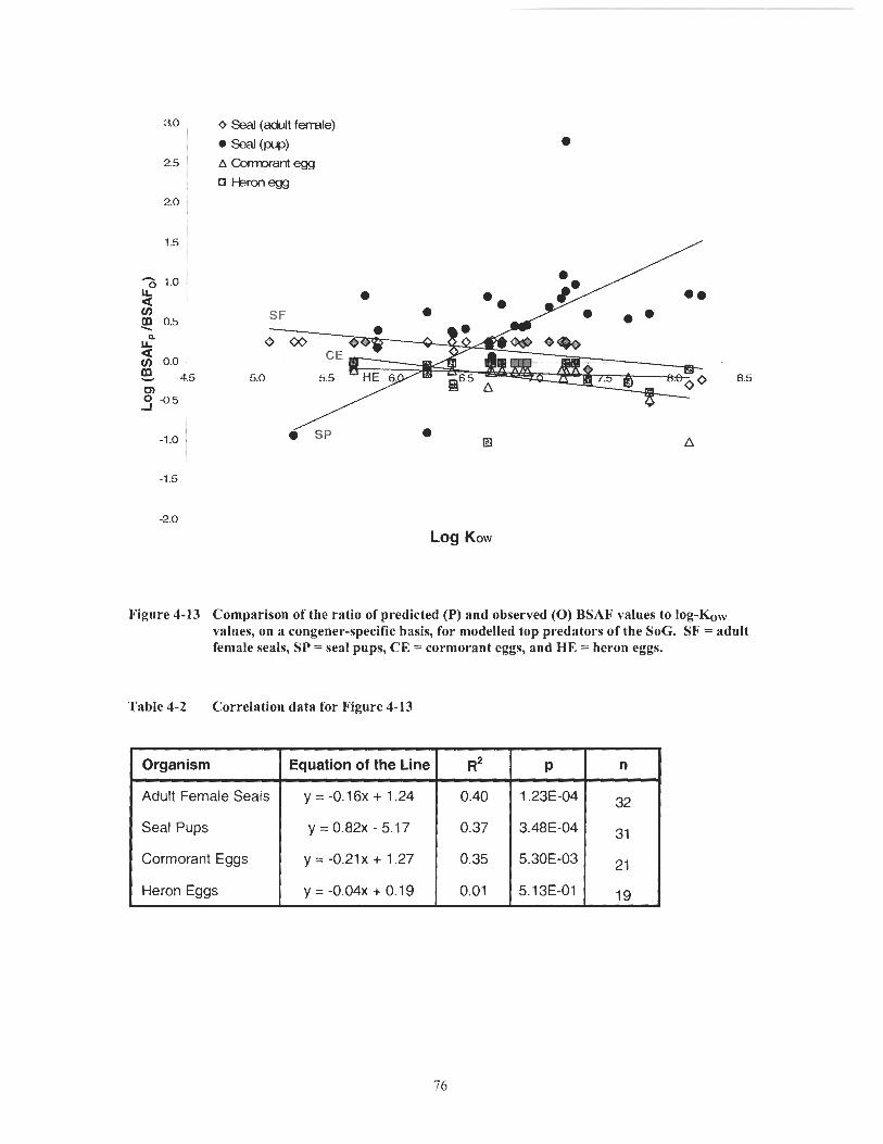
3.0 ,
25 '
2.0
1.5 1
I
h 1.0
2 V) m 0.5 \
P
2 V) 0.0
4.5 m g -0.5
1
-1 .o
-1.5
-2 0
Figure 4-13
Table 4-2
0 Soal (adult fenale)
s@A (pup) A Cornwant egg
0 Mron egg
. El A
Log Kow
Comparison of the ratio of predicted (P) and observed (0) BSAF values to log-Kow values, on a congener-specific basis, for modelled top predators of the SoC. SF = adult female seals, SP = seal pups, CE = cormorant eggs, and HE = heron eggs.
Correlation data for Figure 4-13
Organism I Equation of the Line I R~
Adult Female Seals
Seal Pups
Cormorant Eggs
Heron Eggs
y = -0.16~ + 1.24
y = 0 .82~ - 5.1 7
y = -0.21~ + 1.27
y = -0.04~ + 0.19
0.40
0.37
0.35
0.01

4.3.2 Model Performance Analysis for ZPCBs
Fibwre 4- 14, which coinpares predicted and observed BSAFs on a CPCB basis, indicates
that predicted BSAFs for adult female seals, cormorant eggs, and heron eggs all fall
within two standard deviations of the observed geometric mean, while predicted BSAFs
for seal pups fall slightly above the observed range. Table 4-3, which shows the CPCB
MB results for seals and birds, illustrates that the model over-predicts the BSAF on a
ZPCB basis for adult female seals and seal pups (MB = 1 .GO and 3.18, respectively) and
slightly under-predicts the BSAF on a ZPCB basis for cormorant and heron eggs (MB =
0.73 and 0.8 1, respectively). These results generally agree with the results of the
performance analysis done on a congener specific basis. above.
0 Redictd
na-served
Cormrant eggs EPCBs
Figure 4-14 Predicted and observed BSAFs (glg) of CPCBs for seal pups, adult female seals, cormorant eggs, and heron eggs from the SoC. Error bars represent two standard deviations of the observed geometric mean (n = 10 for seal pups, 4 for adult female seals, 19 for cormorant eggs, and 12 for heron eggs)
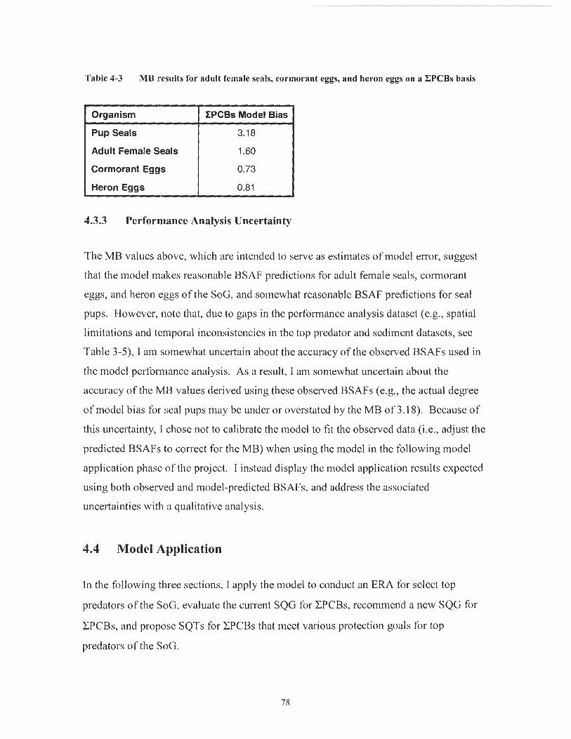
Table 4-3 MB results for adult female seals, cormorant eggs, and heron eggs on a ZPCBs basis
4.3.3 Performance Analysis Uncertainty
Organism
Pup Seals
Adult Female Seals
Cormorant Eggs
Heron Eggs
The MB values above, which are intended to serve as estimates of model error, suggest
that the model makes reasonable BSAF predictions for adult female seals, cormorant
eggs, and heron eggs of the SoG, and somewhat reasonable BSAF predictions for seal
pups. However, note that, due to gaps in the performance analysis dataset (e.g., spatial
limitations and temporal inconsistencies in the top predator and sediment datasets, see
Table 3-9 , I am somewhat uncertain about the accuracy of the observed BSAFs used in
the model performance analysis. As a result, I am somewhat uncertain about the
accuracy of the MB values derived using these observed BSAFs (e.g., the actual degree
of model bias for seal pups may be under or overstated by the MB of 3.18). Because of
this uncertainty, I chose not to calibrate the model to f i t the observed data (i.e., adjust the
predicted BSAFs to correct for the MB) when using the model in the following model
application phase of the project. I instead display the model application results expected
using both observed and model-predicted BSAFs, and address the associated
uncertainties with a qualitative analysis.
ZPCBs Model Bias
3.18
1.60
0.73
0.81
4.4 Model Application
In the following three sections, I apply the model to conduct an ERA for select top
predators of the SoG, evaluate the current SQG for CPCBs, recommend a new SQG for
CPCBs, and propose SQTs for CPCBs that meet various protection goals for top
predators of the SoG.

4.4.1 Ecological Risk Assessment
4.4.1.1 ERA for Adult Female Seals
Figure 4-15 shows the observed and model predicted distributions of CPCB
concentrations (ndg-lipid) in adult female seals of the SoG in relation to the effects
threshold. The observed distribution ranges from a log-CPCB concentration of
approximately 2.7 to 3.8 nglg-lipid, while the model predicted distribution ranges fkom a
log-CPCB concentration of approximately 2.7 to 4.3 ng/g-lipid. Figure 4- 15 illustrates
that approximately one percent of the model-predicted adult female seal population, and
no members of the observed adult female seal population, are anticipated to have PCB
body burdens that exceed the log-CPCB effects threshold of 4-06 ng/g-lipid.
25 3.0 3.5 Log tPCBs (nglg lipid) in Female Seals
Figure 4-15 The predicted and observed distribution (n = 4) of CPCB concentrations (nglg lipid) in adult female seals in relation to the effects threshold. The solid and dashed curves depict the predicted and observed CPCB distributions, respectively. The horizoiltal dotted line marks the effects threshold. The circled value indicates the proportion of adult female seals in the SoG predicted to have CPCB concentrations above the threshold.
Given that nearly the entire CPCB concentration distribution for observed and predicted
adult female seals lies below the effects threshold (Figure 4-15), it appears that the risk of
adverse effects associated with PCB exposure to adult female seals in the SoG is low.
However, note the following uncertainties associated with this risk characterization.
First, it is not clear to what extent the observed CPCB distribution for adult female seals,
which is based on four seals from Vancouver Airport, represents the actual CPCB
distribution for adult female seals throughout the entire SoG. Second, given the lack of
model input and performance analysis data (Table 3-4 and Table 3-5), the MB of 1.60 for
adult female seals, and the use of the cormorant egg SD to derive the variability for the
predicted distribution. it is not clear to what extent the predicted distribution represents
the actual CPCB distribution for adult female seals throughout the entire SoG. Finally,
given the TRV data gaps (Table 3-7) and the uncertainties associated with the effects
threshold [Kannan et al., 20001, it is not clear to what extent the effects threshold in
Figure 4- 15 represents the actual CPCB effects threshold for adult female seals
throughout the SoG. Therefore, though the risk of adverse effects associated with PCB
exposure to adult female seals in the SoG appears to be low, the possibility of adverse
effects to a significant proportion of the adult female seal population cannot be ruled out.
4.4.1.2 ERA for Seal Pups
Figure 4-1 6 shows the observed and model predicted distributions of CPCB
concentrations (nglg-lipid) in seal pups of the SoG in relation to the effects threshold.
The observed distribution ranges from a log-CPCB concentration of approximately 2.75
to 4.0 ndg-lipid, while the model predicted distribution ranges from a log-CPCB
concentration of approximately 3.1 to 4.6 ndg-lipid. Figure 4- 16 illustrates that
approximately thirty-one percent of the model-predicted seal pup population, and no
members of the observed seal pup population, are anticipated to have PCB body burdens
that exceed the log-CPCB effects threshold of 4.06 ng/g-lipid.

Effects threshold
Log XPCB; (nglg lipid) in Pup Seals
Figure 4-16 The predicted and observed distribution (n = LO) of CPCB concentrations (nglg lipid) in seal pups in relation to the effects threshold. The solid and dashed curves depict the predicted and observed ZPCB distributions, respectively. The horizontal dotted line marks the effects threshold. The circled value indicates the proportion of seal pups in the SoC predicted to have ZPCB coi~ceritrations above the threshold.
The ERA result for seal pups (Figure 4-16) suggests that the risk of adverse effects
associated with PCB exposure to seal pups in the SoG is low to moderate. However, note
the following uncertainties associated with this risk characterization. First, it is not clear
to what extent the observed CPCB distribution for seal pups, which is based on ten seals
from Hornby Island, represents the actual CPCB distribution for seal pups throughout the
entire SoG. Second, given the lack of model input and perfotmance analysis data (Table
3-4 and Table 3-5), the MB of 3.18 for seal pups, and the use of the cormorant egg SD to
derive the variability for the predicted distribution, it is not clear to what extent the
predicted distribution represents the actual CPCB distribution for seal pups throughout
the entire SoG. Finally, given the fact that effects threshold used was derived for adult
seals and is associated significant uncertainty itself [Kannan et al., 20001, it is not clear to
what extent the effects threshold in Figure 4-1 6 represents the actual CPCB effects
threshold for seal pups throughout the SoG. Therefore, though the risk of adverse effects
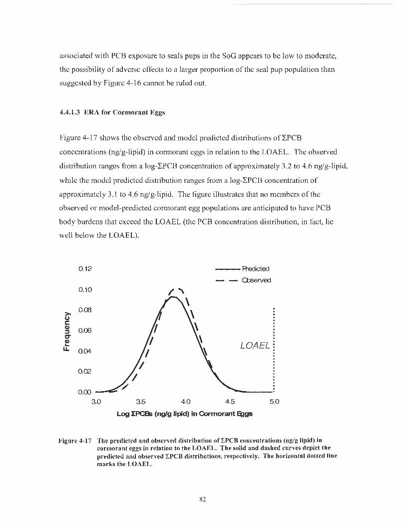
associated with PCB exposure to seals pups in the SoG appears to be low to moderate,
the possibility of adverse effects to a larger proportion of the seal pup population than
suggested by Figure 4- 16 cannot be ruled out.
4.4.1.3 ERA for Cormorant Eggs
Figure 4- 17 shows the observed and model predicted distributions of CPCB
concentrations (ng/g-lipid) in cormorant eggs in relation to the LOAEL. The observed
distribution ranges from a log-CPCB concentration of approximately 3.2 to 4.6 ng/g-lipid,
while the model predicted distribution ranges from a log-CPCB concentration of
approximately 3.1 to 4.6 ng/g-lipid. The figure illustrates that no members of the
observed or model-predicted cormorant egg populations are anticipated to have PCB
body burdens that exceed the LOAEL (the PCB concentration distribution, in fact, lie
well below the LOAEL).
3.0 3.5 4.0 4.5 5.0
Log W C B B (nglg lipid) in Cormorant ags
Figure 4-17 The predicted and observed distribution of CPCB co~~ce~~tri i t ions (nglg lipid) in cormorant eggs in relation to the LOAEL. The solid and dashed curves depict the predicted and observed CPCB distributions, respectively. The liorizontal dotted line marks the LOAEL.

The ERA result for cormorant eggs (Figure 4- 17) suggests that the risk of adverse effects
associated with PCB exposure to cormorant eggs in the SoG is low. My confidence in
this risk characterization is somewhat high mainly because my confidence in the
observed distribution (which is based on a strong dataset) and predicted distribution
(which closely matches the observed distribution) is high. However, because the TRV
used in the assessment is a LOAEL rather than an effects threshold, is a point estimate,
and is based on studies with non-SoG organisms [Hoffman et a!., 19961, the possibility of
adverse effects associated with PCB exposure to at least some members of the cormorant
egg population in the SoG cannot be ruled out.
4.4.2 Sediment Quality Guideline Evaluation and Recommendation
4.4.2.1 SQC Definition
SQGs "apply province-wide and are safe levels of substances for the protection of a given
water use, including drinking water, aquatic life, recreation and agricultural uses" [MOE,
20061. It is unclear what the MOE considers to be a "safe level" of exposure; however,
Dr. Glyn Fox of the MOE indicated that water quality guidelines are typically set to
protect aquatic organisms to the NOAEL [Dr. Glyn Fox, MOE, personal
communication].
4.4.2.2 SQG Evaluation
The SQG for CPCRs is set to a maximum value of 2.0 pg/g organic carbon (OC) [MOE,
20061. This guideline is based on a combination of (i) PCB exposure and effects data
from laboratory studies conducted primarily on freshwater fish and invertebrates, (ii) the
application of simple equilibrium partitioning equations, and (iii) the application of
uncertainty factors [Nagpal, 19921. Given that little, if any, SoG-specific exposure and
effects data was used to derive the SQG, and given the large BSAFs predicted for the
system (Figure 4-2), it is unclear whether the current SQG for CPCBs does indeed result
in safe levels of PCBs in aquatic organisms of the SoG.

Figure 4-1 8 shows a comparison of the CPCB concentration associated with the SQG
(i.e., the CB-SOG, which was derived by multiplying the SQG by the model-predicted
BSAF) to the predicted CPCB concentration distribution, observed CPCB concentration
distribution, and TRVs for cormorant eggs, adult female seals, and seal pups of the SoG.
This figure illustrates that the SQG for CPCBs is expected to result in a CPCB
concentration (the blue arrows with the CB.sQG identifier) that is 6.3 times above the
NOAEL for adult female seals, 12.6 times above the NOAEL for seal pups, and at the
LOAEL and above the NOAEL for cormorant eggs. The CB-SQG is also well above the
effects threshold for adult female seals and seal pups. Note that multiplication of the
SQG by the observed BSAF for each organism also results in exceedances of the NOAEL
and effects threshold for adult female seals and seal pups, and a match of the LOAEL for
cormorant eggs (results not shown). These results suggest that the SQG for CPCBs does
not result in safe levels of PCBs in seals or cormorant eggs of the SoG, and thus the
current SQG may not be adequate to meet the MOE's protcction goals.
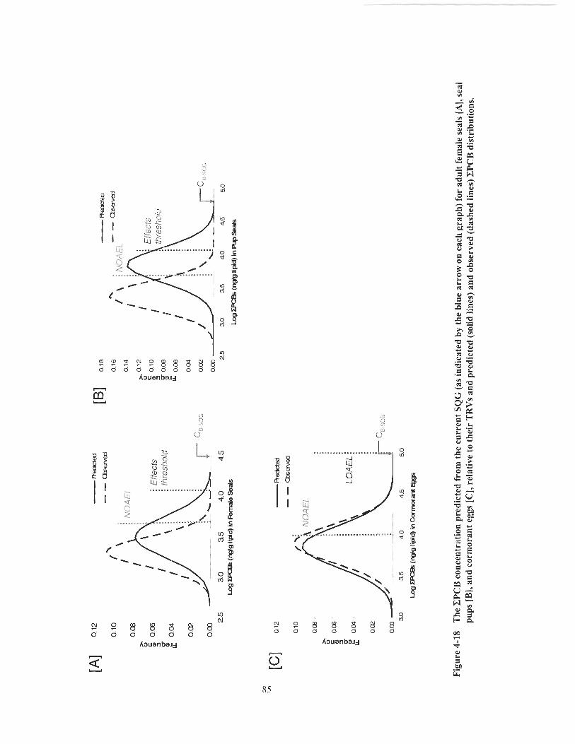
[A]
0.12
30 " [C]
0.12 25
3.
0 3.5
4.
0 4.5
Log
(ng'
g lip
ld) i
n k
md
e Seds
Log
(ng
lg li
pid
) in C
orm
ora
nt
[B]
a18
-Ftedcted
25
3.0
3.5
4.0
4.5
5.0
Log
(ng'
g lip
id) I
n h
p Seals
Fig
ure
4-18
T
he C
PC
B c
once
ntra
tion
pre
dict
ed fr
om th
e cu
rren
t SQ
G (a
s in
dica
ted
by t
he b
lue
arro
w o
n e
ach
grap
h) fo
r ad
ult f
emal
e se
als
[A],
seal
pu
ps [
B],
and
cor
mor
ant
eggs
[C
], r
elat
ive
to th
eir
TR
Vs
and
pred
icte
d (s
olid
line
s) a
nd o
bser
ved
(das
hed
lines
) CP
CB
dis
trib
utio
ns.

Figure 4-1 9 shows the distribution of CPCB concentrations (ng/g-lipid) in adult female
seals (A) and cormorant eggs (B) that would be expected if the geometric mean CPCB
concentration in sediments of the SoG were at the SQG. The dashed and solid
distribution in each graph were derived by multiplying the SQG for CPCBs by the
observed and model-predicted BSAF, respectively. For adult female seals, the majority
of both CPCB concentration distributions exceed threshold effects level, while for
cormorant eggs, about half of both CPCB concentration distributions exceed the LOAEL.
These results further suggest that the SQG for CPCBs does not result in safe levels of
PCBs in adult female seals or cormorant eggs of the SoG, and thus the current SQG may
not be adequate to meet the MOE's protection goals.

3.5 4.0 4.5 5.0 5.5
Log P C 5 (nglg lipld) In Female Seals
. - - Observed
3.5 4.0 4.5 5.0 5.5 6.0
Log I P C 5 (nglg lipid) in Cormorant Eggs
Figure 4-19 The ZPCB co~rceirtration distribution predicted by multiplying the current SQG by the observed (dashed line) and predicted (solid line) BSAFs for adult female seals [A] and cormorant eggs [B] relative to their TRVs.
4.4.2.3 SQG Evaluation Uncertainty
There exists some uncertainty about the accuracy of the observed and predicted BSAFs
used to estimate the CPCB concentrations in Figure 4-1 8 and Figure 4-1 9 (see Section
4.3.3). As a result, there exists some uncertainty about the extent to which the CPCB
concentrations in top predators of the SoG associated with the SQG would, in the field,
actually exceed the TRVs for these organisms. However, given the degree of the TRV
exceedances estimated with both the observed and model-predicted BSAFs (Figure 4-1 8
and Figure 4-19), the uncertainties about the accuracy of the TRVs (Section 3.3.2 and
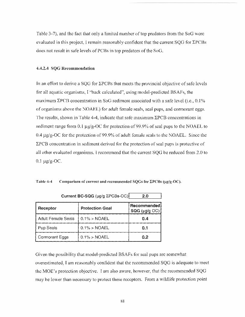
Table 3-7), and the fact that only a limited number of top predators from the SoG were
evaluated in this project, I remain reasonably confident that the current SQG for CPCBs
does not result in safe levels of PCBs in top predators of the SoG.
4.4.2.4 SQG Recommendation
In an effort to derive a SQG for CPCBs that meets the provincial objective of safe levels
for all aquatic organisms, I "back calculated", using model-predicted BSAFs, the
maximum CPCB concentration in SoG sediment associated with a safe level (i.e., 0.1%
of organisms above the NOAEL) for adult female seals, seal pups, and cormorant eggs.
The results, shown in Table 4-4, indicate that safe maximum CPCB concentrations in
sediment range from 0.1 yg/g-OC for protection of 90.0% of seal pups to the NOAEL to
0.4 pg/g-OC for the protection of 99.9% of adult female seals to the NOAEL. Since the
CPCB concentration in sediment derived for the protection of seal pups is protective of
all other evaluated organisms, I recommend that the current SQG be reduced from 2.0 to
0.1 yglg-OC.
Table 4-4 Comparison of current and reconinie~ided SQGs for CPCBs (pglg-OC).
Current BC-SQG (pglg ZPCBS-OC)I 2.0
1 Adult Female Seals 1 0.1 % > NOAEL I 0.4 1 Receptor Protection Goal
Pup Seals
Given the possibility that model-predicted BSAFs for seal pups are somewhat
overestimated, I am reasonably confident that the recommended SQG is adequate to meet
the MOE's protection objective. I am also aware, however, that the recommended SQG
may be lower than necessary to protect these receptors. From a wildlife protection point
Recommended SQG (clsfs oc)
Cormorant Eggs
0.1 % > NOAEL 0.1
0.1 % > NOAEL 0.2
of view, a SQG for CPCBs that is unnecessarily low may be defensible. PCBs are only
one of the contributing stressors to ecological receptors in the SoG (others include POPS
and other chemicals, habitat destruction, reduced prey availability, etc.), and the SoG
food web potentially extends to higher trophic levels (e.g., to the endangered and
declining population of orcas) which could be subject to higher PCB doses than seals and
cormorants are. Furthermore, a conservatively low SQG for the protection of seal pups
may be warranted, in this case, given the uncertainty associated with the PCB body
burdens in, and related health effects to, seal pups and seal foetuses.
4.4.3 Sediment Quality Target Proposals
4.4.3.1 SQT Definition
A SQT (also known as a sediment quality objective) is a level of a given substance in
sediment that one aims to achieve. This level can be a single value (e.g., a maximum
value like the SQG) or a distribution of values. SQTs are typically site-specific (i.e., they
do not necessarily apply province wide) and can be set to achieve whatever protection
endpoint is desired (e.g., no more than 10% of the seal pup population in the SoG shall be
exposed to CPCBs in concentrations that exceed their effects threshold). I am not aware
of any provincial or federal SQT for CPCBs in the SoG.
4.4.3.2 SQT Proposals
In an effort to guide provincial and federal environment managers to SQTs that meet
protection goals for top predators of the SoG, I "back calculated", using model-predicted
BSAFs, maximum allowable CPCB concentrations in sediment associated with a variety
of protection outcomes for seals and cormorant eggs. Note that it would be more useful
to express the proposed SQTs as distributions rather than maximum values. However,
my uncertainty about the relationship between the distribution of PCB concentrations in
sediments and top predators of the SoG is too high to derive SQT distributions with any
reasonable degree of confidence. The results of my SQT derivation, shown in Table 4-5,

indicate that proposed SQTs range from a CPCB concentration of 0.4 pg/g-OC (5% of
seal pups above the NOAEL) to 6.0 pg/g-OC (5% of cormorant eggs above the LOAEL).
Table 4-5 Proposed sediment quality targets for ZPCBs (&g-OC) for the protection of seals and marine birds in the SoC.
I 5% > NOAEL I 1.0
Receptor
Adult Female Seals 1 5% > Effects Threshold 1 1.9
Protection Goal
Pup Seals 1 5% > Effects Threshold I 1.0
Recommended SQT (IJgIg OC)
5% > LOAEL
5% > NOAEL
5% > LOAEL
0.1 % > LOAEL Cormorant Eggs
5% > LOAEL
4.8
0.4
Given that model-predicted BSAFs for seal pups and adult female seals may be
somewhat overestimated (i.e., they have MB values of 3.18 and 1.60, respectively), I am
reasonably confident that the proposed SQTs for these organisms are adequate to meet
the desired protection goal. Given that the model-predicted BSAF for cormorant eggs is
associated with an MB of 0.73, the SQT for this organism may be slightly high.
CONCLUSIONS & RECOMlMENDATIONS
5.1 Project Summary
In an effort to enhance the understanding of POP-bioaccumulation dynamics in the SoG
and improve the decision-making capacity of environmental managers, I (i) developed,
parameterized, and tested a mechanistic bioaccumulation model for PCBs in the SoG; (ii)
used this model to help conduct an ERA for the SoGYs top predators, assess the adequacy
of the current SQG for CPCBs, propose a new SQG, and propose a range of SQTs; and
(iii) identified gaps in the data required to support the development, testing, and
application of the bioaccumulation model. The results of these project phases are
summarized below.
Model performance analysis indicates that model-predicted BSAFs for CPCBs in
cormorant eggs, heron eggs, and adult female seals are in reasonable agreement
with observed BSAFs (MB values are 0.73, 0.8 I , and 1.60, respectively), while
model-predicted BSAFs for seal pups are potentially overestimated (MB = 3.18).
The performance analysis dataset for these organisms was limited spatially,
temporally, chemically, and statistically (Table 3-5), however, and thus the model
was not calibrated to fit the observed data before the model application phase of
the project.
The ERA estimated that virtually no members of the cormorant egg or adult
female seal population in the SoG have CPCB body burdens in excess of their
LOAEL (Figure 4- 17) and effects threshold (Figure 4- 1 9 , respectively. The ERA
also estimated that virtually no members of the observed seal pup population (i.e.,
that from Hoi-nby Island) and 3 1 % of the model-predicted seal pup population
have CPCB body burdens in excess of their effects threshold (Figure 4-16).
Based on these results, the ERA concluded that risks associated with current

levels of PCB exposure to cormorant eggs and adult female seals are probably
low, while risks to seal pups are probably low to moderate. It was acknowledged,
however, that given the gaps in the empirical dataset (e.g., empirical seal
concentrations for the entire SoG, appropriate TRVs, etc. - see Table 3-4, Table
3-5, and Table 3-7), the possibility of adverse effects to a larger proportion of
these top predator populations than indicated by the ERA cannot be definitively
ruled out.
Evaluation of the SQG for CPCBs suggests that if CPCB concentrations in SoG
sediments were equivalent to the SQG, CPCB body burdens in a large portionof
the population of adult female seals, seal pups, and cormorant eggs would exceed
their NOAELs for CPCBs and, possibly, their threshold effects levels as well. As
a consequence, the MOE's goal of protecting all aquatic organisms in BC to the
NOAEL would not be achieved with the current SQG for CPCBs.
The proposed SQG that is expected to protect all organisms investigated to the
NOAEL is approximately 0.1 pg/g-OC, a value that is 20 times lower than the
current SQG of 2.0 pg/g-OC.
The proposed SQTs for the protection of top predators in the SoG to various
ecological endpoints range from a CPCB concentration of 0.4 pdg-OC (5% of
seal pups above the NOAEL) to a CPCB concentration of 6.0 pglg-OC (5% of
cormorant eggs above the LOAEL).
The main gaps in the project's data include the following: 6 1 5 ~ values for
organisms of the SoG diet matrix, kM values for birds and seals, PCB
concentrations in sediments and biota of the SoG, TRVs for most organisms of
the food web, and a various model parameter values.
5.2 Key Findings and Implications
The first key finding is that the current SQG for CPCBs does not appear to protect top
predators in the SoG to the NOAEL or, potentially, to the threshold effects level (Section
4.4.2.2). This finding suggests that the current approach used by the MOE to derive
SQGs for PCBs does not adequately account for the degree of PCB biomagnification in
the resident food web of the SoG (i.e., potentially a 500-fold increase in CPCB
concentrations from sediment (dw) to seal pups (ww) (Section 4.2)). It is unclear
whether this is of concern for the management of wildlife exposure to PCBs in the SoG.
Current PCB levels in the SoG, which are not expected to increase, appear to pose low
risks to the SoG's resident top predators (Section 4.4.1); however, they may not pose low
risks to BC orcas which occupy a higher trophic position than seals, have high PCB body
burdens, and are experiencing population declines [Ross et al., 20001. Regardless, the
lack of accounting for PCB biomagnification in the SoG is a concern for the management
of the thousands of currently unregulated POPs. Derivation of inappropriate SQGs for
POPs could lead to POP body burdens in BC's top predators that exceed effects
thresholds for individual POPs, which is inconsistent with the environmental protection
goals of the province. For POPs with similar modes of toxicity (i.e., PCBs, PBDEs,
PC.DDs, furans, etc), the degree of threshold effects exceedance, and the associated risks
to the health of wildlife and humans in BC, could be substantial.
The second key finding is that there are significant gaps in the set of empirical data
required for model development, model performance analysis, and model application
(Table 3-4, Table 3-5, and Table 3-7). These data gaps affect the confidence in the
model-predicted BSAFs - e.g., confidence in the accuracy of the model-predicted BSAF
for hake is low because the observed PCB concentration data for hake, required for
model performance analysis, were not available. The data gaps also limit the extent to
which I could apply the model-predicted BSAFs to address management issues - e.g., I
could not assess the risks of PCB exposure to herons or assess the adequacy of the current
SQG for their protection because I lacked heron TRVs. In addition, the data gaps
affected my confidence in the model application results - e.g., I could not state with

confidence whether any seal pups in the SoG are expected to have CPCB body burdens
that exceed their CPCB effects threshold because I lacked appropriate empirical PCB
concentration data for pups from throughout the SoG and because I lacked pup-specific
TRVs.
The impact of data gaps on the level of confidence in the model is important because the
level of confidence in the model ultimately affects the ability of risk managers to make
model-informed decisions. For example, the lack of data on the distribution of PCB
concentrations in hening, salmon, and hake limits the ability of the model to estimate,
with confidence, the relative contribution of immigrant and resident organisms to PCB
body burdens in seals. This, in turn, could hamper a manager's ability to control seal
exposure to PCBs by leading to the misallocation of funds between programs aimed at
reducing PCB body burdens in immigrant organisms (e.g., via the pursuit of international
pollution abatement agreements) and programs aimed at reducing PCB body burdens in
resident organisms (e.g., by the remediation of local sediments). While the influence of
data gaps on model confidence and ultimately management decisions may not be of
concern for the management of seal exposure to PCBs (note that risks to resident
organisms appear to below (Section 4.4.1)), it may certainly be of concern for the
management of sea1 and other top predator exposure to the broad class of emerging
POPS, particularly those with synergistic modes of toxicity.
5.3 Recommendations
The MOE should revise its methodologv for deriving SOGs for POPs
The results of this project suggest that the methodology used by the MOE to derive SQGs
for CPCBs does not adequately account for the degree of PCB bionlagnification in the
SoG food web. As a result, the SQG goal of ensuring safe levels of PCBs for the
protection of aquatic life [MOE, 20061 is likely not being met by the current SQG for
PCBs. To avoid the derivation of inappropriate SQGs for other POPs, I recommend that
the MOE revise its SQG derivation methodology for POPs. Specifically, I recommend

that the MOE continue to support the development of, and use, POP bioaccumulation
models such as the one developed here for PCBs. Note that this model can potentially be
adapted to derive SQGs for other POPS (e.g., PBDEs).
GBAP should reduce gaps in the PCB bioaccumulation datasets
The GBAP aims to improve the capacity of environmental managers to make decisions
by advancing scientific understanding [Environment Canada, 20051. The scientific
understanding of PCB bioaccumulation dynamics in the SoG is, as this project
determined, limited due to the lack of data required for model parameterization, testing,
and application. As a result, the capacity of environmental managers to make cost-
effective decisions aimed at reducing potential PCB exposure risks to wildlife is currently
limited. To reduce uncertainty in the model and improve its utility for making
management decisions, I recommend that the GBAP direct more efforts towards
narrowing the gaps in the empirical datasets. Included below are the key data gaps, listed
in order of highest to lowest research priority, that should be addressed.
1 . PCB Concentrations in Sediment. The current dataset of PCB concentrations in
sediment is deficient spatially (data is from the central SoG and Howe Sound
only), temporally (data are from 1997), chemically (concentrations for only 34
congeners were reported), and statistically (n = 3). These deficiencies affect all
phases of the project and are ultimately the greatest source of doubt about model
accuracy. Resources should be directed at improving the sediment PCB
concentration database through increased sampling, improved chemical analysis,
andlor increased publication of existing data.
2. PCB Concentrations in Organisms. The current dataset of PCB concentrations in
herring and salmon is deficient spatially (i.e., f?om limited and unknown regions
of the SoG, respectively) and statistically (n = 2 and 3, respectively). The current
datasets of PCB concentrations in organisms used for model performance analysis
are deficient temporally (bird data is from the 1990s), spatially (seal and fish data
are from geographically small areas of the SoG), chemically (congener data is
limited for all organisms except seals), and statistically (sample sizes are small for
adult female seals, fish, and invertebrates). In addition, performance analysis data
is missing for a number of organisms (i.e., plants, invertebrates, most fish, adult
male seals, juvenile seals, seal foetuses, etc.) and for related seal pups and
mothers. All these data gaps reduce confidence in the results of the development,
performance analysis, and application phases of the project. As a second priority,
resources should be directed at improving the empirical performance analysis
dataset. Particular attention should be paid to improving the datasets of hake,
herring, and seals since thesc are especially important for characterizing PCB
bioaccumulation to seals. As above, this can be accomplished through increased
sampling or increased publication of existing data.
3. 615N Data. The current diet matrix (Table 3- I), based on observational studies
and scat collection, appears to reasonably represent feeding relationships
throughout the SoG. However, the lack of spatially diverse 61 5N data for most
organisms of the matrix makes verification of the matrix's accuracy difficult.
Given the strong link between TP and POP concentration [Mackintosh et a].,
2004; Fisk et al., 2001; Burreau et al., 20041, resources should be directed to
improving the picture of feeding relationships in the SoG through collection and
analysis of more 61 5N data (note that 61 5N analysis is relatively inexpensive).
Improvements in understanding SoG feeding relationships may be particularly
important as the SoG ecosystem changes with increased anthropogenic
interference (i.e., fishing, tourism, trade, etc.) and climate change.
4. Toxicity Data. The toxicity dataset is limited to a point value NOAEL and
LOAEL for adult seals and cormorant eggs. Moreover, there is considerable
uncertainty associated with these point value TRVs, particularly when
extrapolated from non-SoG organisms in captivity to SoG organisms in the wild.
These data gaps limit the accuracy of and confidence in the results of the model
application phase of the project. For instance, because toxicity data for seal pups

and foetuses is missing, the potential health risks to these organisms associated
with PCB exposure are not clear. Improving the toxicity database is ranked fourth
in research priority because it affects only the model application phase of the
project and because conservative assun~ptions can be used to fill these data gaps
for the moment.
5. Model Parameter Data. A number of parameter values are based on limited
empirical data (e.g., OC content of sediment, body temperatures of birds and
seals, growth rate constant for phytoplankton, etc.) or were simply estimated (seal
kM values, water fraction in crabs, etc.) - see appendices Section 7.4. Errors in
parameter values primarily affect the model development (i-e., BSAF predictions)
phase of the project. As a group, these data are ranked fifth in research priority
because the benefit/cost ratio associated with improving them is lower than that
associated with improving the datasets above.
Note that, regardless of whether wildlife exposure to PCBs is still of management
concern, it remains important to address the PCB-relevant data gaps above (i.e., #1,2,
and 5) because all future POP modelling will depend on, and be affected by, the quality
of the bioaccumulation model for PCBs.
GBAP should improve the data collection and management framework
As discussed above, there are considerable gaps in the PCB bioaccumulation datasets.
As a result, significant funds will likely be required to obtain the amount of PCB and
other POP bioaccumulation data necessary for well-informed decision making by risk
managers. In order to get the most out of limited data collection funds, I recommend that
GBAP promote data collection efficiencies by encouraging, and earmarking funds for,
data collectors to obtain additional data during their research that is not of direct interest
to them but is of interest to the broader scientific and management objectives of GBAP.
For instance, a researcher collecting heron eggs for PBB analysis could be given
additional funds to collect proximate sediment, soil, and heron prey samples, and analyze

these for lipid content, 61 5N values, various POPS of concern, etc. This use of funds will
be cheaper in the long run than making numerous different excursions for each of these
types of data. It also addresses some of the temporal and spatial limitations of current
bioaccumulation datasets.
Further to making the above efficiency improvements, the GBAP should establish a data
inventory where data collection priorities can be made explicit, and where data collection
results can be organized and posted. This will help data collectors to identify data
requirements, modellers to improve the accuracy of their models, and the GBAP to avoid
funding work that has already been done.

6 APPENDICES
6.1 Diet Matrix Verification Data
Table 6-1 The estimated annual average diet of harbour seals in the SoC [from Olesiuk, 19931
Pacific hake Pacific herring Salmonids Plainfin midshipman Lingcod Surf perches Cephalopods (i.e., squid) Flatfish species Sculpins Rockfish Pacific tomcod JValleye pollock Pacific sand lance Pacific cod Smelts (mainly eulachon) Unidentified / other fishes 3ther invertebrates
Total
Lower - upper limit (% mass)
na na na
misc. demersal mi%. demersal misc. demersal small pelagic
misc. demersal misc. demersal misc. demersal mi%, demersal
na small pelagic
rnisc. demersal small pelagic
na na

Table 6-2 SoG diet matrix reported in Pauly Rr Christensen, 1995
Predator Mammals (res.) Large Pelagics Small Pelagics Hake Visc. Demersals Jellies Lg. Macrobenthos Sm. Macrobenthos Sarn. Zooplankton 'lerb. Zooplankton Primary Producers 3irds rransient Orcas Salmon 3etritus
Prev

Table 6-3 Calcr~lated TPs and literature derived 6% ratios for organisms of the SoC feeding
Organism Phytoplankton KelpISea grass H. zooplankton N. plumchrus P. minutus Shellfish Crab Grazing invertebrates C. zooplankton Euphausiids Predatory invertebrates Small pelagic fish (seal prey) Small pelagic fish (bird prey) Lampetra ayresi Misc. demersal fish (seal prey) Misc. demersal fish (bird prey) Hake Dogfish muscle Dogfish liver Dogfish embryo Pollock Leuroglossus English sole DC cormorant (adult) Great blue heron (adult! Seals (adult)
J ~ e a ~ s (juvenile) - 1 = Mackintosh et a/. . 2004
Calculated TP 1 .oo 1 .oo 2.45 2.45 2.45 2.48 3.40 2.78 3.51 2.28 3.56 3.95 3.92 4.60 3.95 3.89 3.57 4.34
3.60 3.49 4.87 4.89 4.89 4.65 4.65
615~%
Mean SD Date
Sampled
Jun-Sep 99
1993
1993; 1999 1993; 1999
1993 1993; 1999 1990; 1993
1999 1999
1999 1999 1999
1 993; 1999 1990
1995; 1996
Sample location
False Creek
SoG
SoG; False Creek SoG; False Creek
SoG SoG; False Creek West Vancouver Island; SoG
False Creek False Creek
False Creek False Creek False Creek
3oG; False Creek 3ulf of Alaska
3ulf of Alaska
2 = Parsons & Lee Chen. 1995 3 = Hobson el al., 1994 4 = Hirons et al. . 2001

6.2 Seal and Bird k*, Values
Table 6-4
PCB Congene:
I 1 v
Estimated seal and bird khl values
Units --:
8
15
1 8130 20128131
37 44/47/65
49169 52
66
61 I?OI?4R6
83/99
9011 01 I1 1 3 105
1101115
118 1281166
12911 3811 60/163
146 14711 49
13511 51 I1 54 1531168 15611 57
170
1 77 18011 93
183/185 187 1 94
19811 99 203 206 209 --
lote: "-" indicates d
Cormorant k, d' '
3.50E-02
3.12E-02
1.00E-03
0.00E+00
1.15E-01
1.20E-02
6.80E-03
1.15E-02
5.20E-03
3.39E-03
1.84E-01
0.00E+00
0.00E+00
0.00E+00
3.00E-03
0.00E+00
8.00E-03 4.4OE-02 0.00E+00
0.00E+00 0.00E+00
I was unavailab
Heron k,, d"
8.00E-03
1.00E-02
0.00E+00
0.00E+00
9.43E-02
4.90E-03
8.50E-04
2.68E-03
1.89E-03
3.70E-03
9.70E-01
0.00E+00
0.00E+00
3.50E-04
0.00E+00
2.79E-03
0.00E+00
0.00E+00 0.00E+00
o estimate this
Seal k,\l d'
2.25E-02
2.95E-01
1.47E-02
2.29E-02
7.80E-01
3.65E-03
7.35E-03
0.00E+00
2.00E-01
8.05E-03
0.00E+00
2.66E-03
2.66E-02
4.43E-02
3.03E-02
7.80E-03
2.25E-03
0.00E+00
2.23E-02
3.46E-03
0.00E+00
6.38E-04
0.00E+00
9.59E-03
0.00E+00
0.00E+00
6.61 E-04 0.00E+00 1.65E-04 0.00E+00 0.00E+00 0.00E+00

6.3 Empirical Model Input Data
Table 6-5 Empirical sediment data used as niodel input (n = 3). Congener numbers in bold were included in the dataset provided by R. Macdonald; congener numbers in brackets are the co-eluting congeners assumed to be represented by the numbers in bold.
PCB Conge~~e,
I I v
Units -- -- 8
15
18 (30)
28/31 (20)
37
44 (47165)
49 (69)
52
66/70
74 (6 1/70/76)
99 (83) 1 01 (9011 13)
105
llO(115)
118
128 (1 66)
38 (12911 601163)
146'
149 (147)
151 (1351154)
153 (1 68)
156 (157)
170 177
180 (1 93)
183 (185)
187
194
199 (1 98)
203
206 209 --
SEDIMENT (11 = 3)
Geometric mean
ng/g tlw
0.04
0.13
0.04
0.36
0.12
0.22
0.19
0.20
0.52
0.13
0.17
0.28
0.17
0.32
0.44
0.11
0.54
0.07
0.36
0.04
0.49
0.02
0.09
0.09
0.14
0.08
0.25
0.03
0.08
0.03
0.05 0.02
na = not applicable Reference: data supplied by Dr. Robie Macdonald
Year collected: 1997
Geometric SD
ng/g dw 0.20
0.21
0.07
0.05
0.09
0.10
0.12
0.1 6
0.05
0.04
0.11
0.1 1
0.1 1
0.1 1
0.14
0.1 1
0.12
na 0.15
0.28
0.11
0.05
0.25
0.16
0.09
na 0.08
na na
na na
PCB 146 valve estimated using Burrard Inlet data (MOE) supplied by the BC M~n~slry of Environment
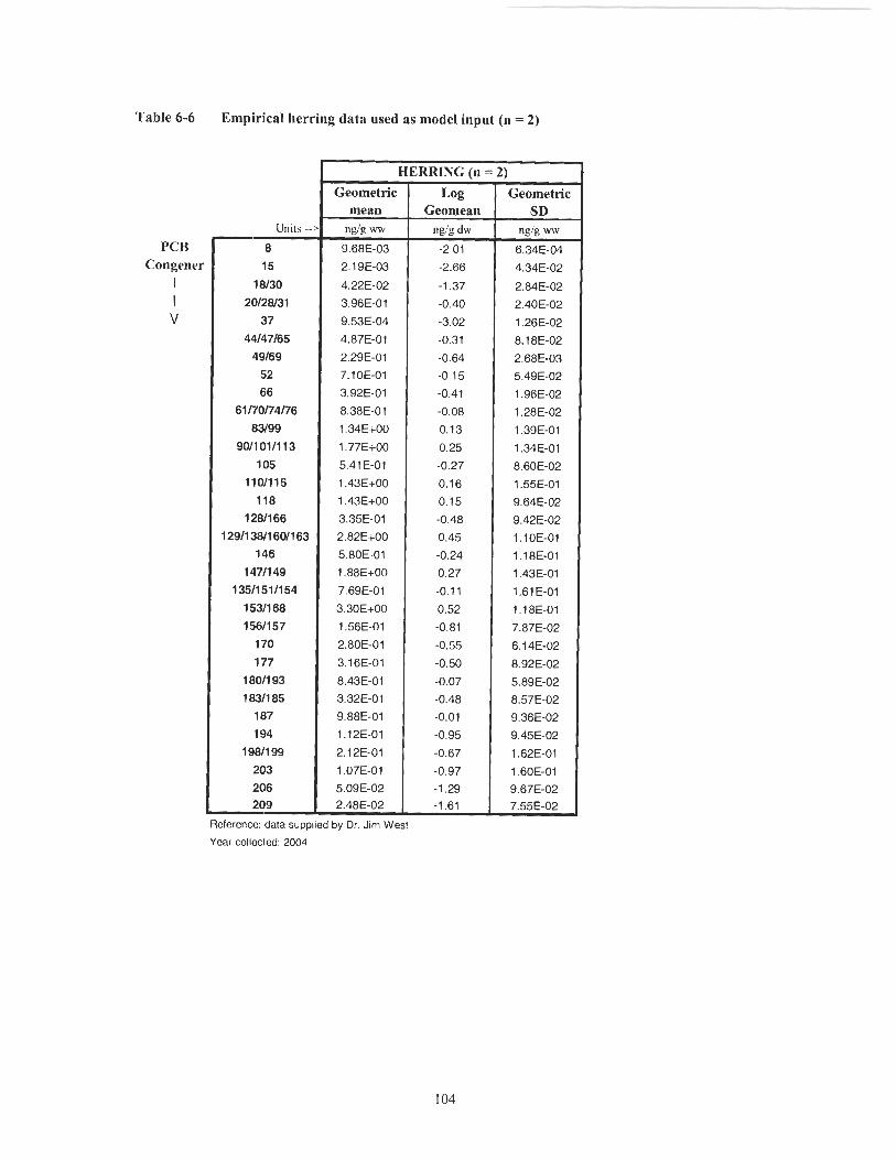
Table 6-6
PCB Con, "ener
I I v
Empirical herring data used as model input (a = 2)
Units - 8
15
18/30
20128131
37
44/47/65
49169
52
66
61ffOI74ff6
83/99
9011 0111 13
105
1101115
118
12811 66
129R 38/1601163
146
14711 49
13511 511154
15311 68
l56/157
170
177
18011 93
18311 85
187
194
19811 99
203
206 209
HERRING (11 = 2) Geometric
mean ng/g ww
9.68E-03
2.19E-03
4.22E-02
3.96E-01
9.53E-04
4.87E-01
2.29E-01
7.10E-01
3.92E-01
8.38E-01
1.34E+00
1.77E+00
5.41E-01
1.43E+00
1.43E+00
3.35E-01
2.82E+00
5.80E-01
1.88E.tO0
7.69E-01
3.30E+00
1.56E-01
2.80E-01
3.16E-01
8.43E-01
3.32E-01
9.88E-01
1.12E-01
2.12E-01
1.07E-01
5.09E-02 2.48E-02
Geomean nglg dw
-2.01
-2.66
-1.37
-0.40
-3.02
-0.31
-0.64
-0.15
-0.41
-0.08
0.13
0.25
-0.27
0.16
0.15
-0.48
0.45
-0.24
0.27
-0.1 1
0.52
-0.81
-0.55
-0.50
-0.07
-0.48
-0.01
-0.95
-0.67
-0.97
-1.29 -1.61
Geometric SD
nglg ww
6.34E-04
4.34E-02
2.84E-02
2.40E-02
1.26E-02
8.1 8E-02
2.68E-03
5.49E-02
1.96E-02
1.28E-02
1.39E-01
1.34E-01
8.60E-02
1.55E-01
9.64E-02
9.42E-02
1.10E-01
1.18E-01
1.43E-01
1.61 E-01
1.18E-01
7.87E-02
6.14E-02
8.92E-02
5.89E-02
8.57E-02
9.36E-02
9.45E-02
1.62E-01
1.60E-01
9.67E-02 7.55E-02
Reference: data supplied by Dr. Jim Wesl
Year collected 2004

Tab
le 6
-7
Em
piri
cal s
alm
on d
ata
used
as
mod
el in
put
(n =
3 f
or a
ll sa
lmon
spe
cies
)
PC
B
Cu
ng
rne~
I I v
CH
UM
(n =
?
Geo
met
ric
SD
nd
g w
5.39
E-0
2
1.11
E-0
1
5.85
E-0
2
7.65
E-0
2
8.60
E-0
2
5.12
E-0
2
3.1
1 E-0
2
3.82
E-0
2
3.77
E-0
2
3.77
E-0
2
1.68
E-0
2
1.30
E-0
2
2.11
E-0
2
5.88
E-0
2
2.16
E-0
2
1.38
E-0
2
1.03
E-0
2
3.34
E-0
2
3.66
E-0
2
6.37
E-0
2
3.15
E-0
2
4.09
E-0
3
3.49
E-0
2
2.58
E-0
2
2.35
E-0
2
3.52
E-0
2
2.42
E-0
2
3.58
E-0
2
2.67
E-0
2
4.71
E-0
2
6.01
E-0
2 8.
08E
-02
Ccw
met
ric
mea
n ng
lg w
8 87
E-0
3
1.50
E-0
3
3.74
E-0
2
7.65
E-0
2
1 .W
E-0
3
5.12
E-0
2
3.1
1 E-0
2
2.34
E-0
1
3.77
E-0
2
3.77
E-0
2
2.18
E-0
1
3.27
E-0
1
6.51
E-0
2
5.88
E-0
2
1.94
E-0
1
1.38
E-0
2
3.14
E-0
1
7.48
E-0
2
2.65
E-0
1
6.37
E-0
2
4.11
E-0
1
4.09
E-0
3
1.46
E-0
2
2.23
E-0
2
5.47
E-0
2
2.63
E-0
2
8.00
E-0
2
5.13
E-0
3
9.94
E-0
3
4.45
E-0
3
2.34
E-0
3 2.
28E
-03
:OH
0 (n
= 3
Log
C
eom
ean
n&'g
dw
-2.0
5
-2.8
2
-1.4
3
-1.1
2
-2.7
2
-1.2
9
-1.5
1
-0.6
3
-1.4
2
-1.4
2
-0.6
6
-0.4
9
-1.1
9
-1.2
3
-0.7
1
-1.8
6
-0.5
0
-1.1
3
-0.5
8
-1.2
0
-0.3
9
-2.3
9
-1.8
4
-1.6
5
-1.2
6
-1.5
8
-1.1
0
-2.2
9
-2.0
0
-2.3
5
-2.6
3 -2
.64
Geo
met
ric
SD
nd
g w
9.07
E-0
2
9.78
E-0
2
1.17
E-0
1
7.65
E-0
2
1.36
E-0
1
5.12
E-0
2
3.1
1 E-0
2
6.61
E-0
2
3.77
E-0
2
3.77
E-0
2
7.74
E-0
2
6.92
E-0
2
1.04
E-0
1
5.88
E-0
2
8.01
E-0
2
1.38
E-0
2
8.64
E-0
2
8.74
E-0
2
7.80
E-0
2
6.37
E-0
2
9.12
E-0
2
4.09
E-0
3
1.09
E-0
1
8.73
E-0
2
9.70
E-0
2
9.38
E-0
2
1.11
E-0
1
1.37
E-0
1
1.35
E-0
1
1.45
E-0
1
1.54
E-0
1 1.
34E
-01
CH
INO
OK
(n
= 3
)
Geo
met
ric
I L
og
I Geo
met
ric
mea
n I
Geo
mea
n I
SD
Ref
eren
ce: d
ata
supp
lled
by D
r. D
avld
0. Car
penl
e~
Year
col
lect
ed: 2
003
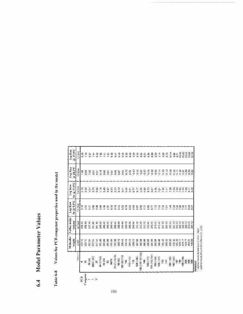

Tab
le 6
-9
E~l
viro
nmen
tal pa
ram
eter
def
init
ions
, val
ues,
and
ref
eren
ces
EN
VIR
ON
ME
NT
AL
PA
RA
ME
TE
RS
-
- - - - - - - - - - - -
- - - - - - - - - - - - - pp pp
Par
amet
er
Sym
bol
Uni
ts
Mea
n SD
n
Ref
eren
ce
Con
cent
ratio
n of
par
ticul
ate
OC
* in
wat
er
Xpo
c kg
/ L
5.65
E-0
7 4.
71 E
-08
6
Est
imat
ed fr
om J
ohan
ness
en e
t (11
. , 20
03
Con
cent
ratio
n of
dis
solv
ed O
C in
wat
er
Xdo
c k@
L
1.32
E-0
6 1.
10E
-07
6
Joha
nnes
sen
et a
l. .2
003
Con
cent
ratio
n of
sus
pend
ed s
olid
s V
ss
kg/L
1.
55E
-05
1.57
E-0
6 -
Est
imat
ed fr
om G
obas
and
Am
ot, 2
005
Wat
er te
mpe
ratu
re
Tw
*C
9.
50E
+00
1.
50E
+00
-
Est
imat
ed f
rom
Dav
enne
and
Mas
son,
200
1 A
ir te
mpe
ratu
re
Ta
OC
1.03
E+
01
5.70
E+
00
12
Est
imat
ed fr
om E
nvir
onm
ent C
anad
a, 2
005
Salin
ity
PSU
gR
f2
3.00
E+
01
2.00
E+
00
- E
stim
ated
from
Fis
heri
es a
nd O
cean
s C
anad
a, 2
003
Den
sity
of O
C i
n se
dim
ent
Foes
kd
L
9.00
E-0
1 -
- G
obas
and
Arn
ot, 2
005
OC
con
tent
of
sedi
men
t O
CS
2.69
E-0
2 1.
38E
-02
6
Joha
nnes
sen
et 1
11. . 20
03
+
Dis
solv
ed o
xyge
n co
ncen
trat
ion
(90%
sat
urat
ion)
C
OX
m
g O
ziL
7.
50E
+00
1.
00E
+00
-
Est
imat
ed F
rom
Paw
low
icz
et (1
1. , 2
003
Sets
chen
ow p
ropo
rtio
nalit
y co
nsta
nt
S-PC
~
icr
n~
1.
80E
-03
- -
Xie
et
(11. , 1
997
Idea
l gas
law
con
stan
t (R
gasl
aw)
RG
L K
8.
31 E
+OO
-
- U
nive
rsal
con
stan
t
Abs
olut
e te
mpe
ratu
re
Tab
s K
2.
73E
+02
-
- U
nive
rsal
con
stan
t
Mol
ar c
once
ntra
tion
of s
eaw
ater
@ 3
5 pp
t M
CS
rnol
/L
5.00
E-0
1 -
- X
ie e
t N
I., 1
997
OC
bur
ial
rate
O
CB
R
gc/c
m2/
yr
1 .l
OE
-02
8.80
E-0
3 6
Joha
nnes
sen
eta
/. , 2
003
Prim
ary
prod
uctio
n ra
te o
f O
C
PP
R
gc/c
m2/
yr
5.5
2~
-01
-
- Pa
uly
et a/. , 1
996
* OC -
orga
nic
carb
on
"-" -
nor
ava
ilabl
e

Tab
le 6
-10
Gen
eral
bio
logi
cal
para
met
er d
efin
itio
ns, v
alue
s, a
nd r
efer
ence
s
GE
NE
RA
L O
RG
AN
ISM
PA
RA
ME
TE
RS
Par
amet
er
Apo
lica
ble
Org
anis
n\s
Svm
bol
Uni
ts
Mea
n S
D
n
Ref
cren
ce
NLOM
- oc
tano
l pr
opor
tton
alit
y co
nsta
nt
,111
G
row
th r
atc
fact
or
Fish
Gro
wth
nte
hct
or
Inve
rteb
rate
s
Pan
icle
sca
veng
ing
cfti
cien
cy
~Mct
abol
ic tran
sfor
mat
ion
rate
Mea
n ho
rneo
ther
mic
teln
pera
ture
Den
sity
of
lipid
s E
w c
onst
ant A
-
P 3
.50
~-0
2
.
- G
obas
n n
1 . 1
999
GR
F.
7.M
E-0
$ j'.a
CjE
-05
- T
hom
ann
el a1 .. I
993
GR
F,
3.50
E-0
4 3.
50E
-05
- T
hom
ann
et a
l..
1992
Filtm
fee
ding
invc
nebr
atcs
IS
- 1.
00E
+00
Plan
ts,
inve
rteb
rate
s, 9
: fi
sh
h,
d-'
0.00
E+
00
Bir
ds &
sea
ls
Bir
ds &
sea
ls
Plan
ts, i
nucn
ebra
tcs,
& k
h
Dcf
aull
valu
e
Arn
ot a
nd G
obas
. 200
4
'r I+
"C
3.
75E
+01
1.
00E
+00
-
Gob
as an
d A
rnot
. 200
5
6 k&
L
9.00
E-0
1 -
- G
obas
and
Arn
ot. 2
005
Ew
A
- 1.
85E
+00
1.
30E
-01
- A
rnot
and
Gob
as. 2
004
Die
tary
abs
orpt
ion
effi
cien
cy o
f lip
id
Zoo
plan
kton
E
l.
7.20
E-0
1 -
- A
rnot
and
Gob
as. Z
OO4
Dic
taly
abs
orpt
ion
effi
cien
cy o
f NL
OM
Z
oopl
ankt
on
7.20
E-0
1 -
- .4
rnot
and
Goh
s. 2
004
Die
tary
abs
orpt
ion
efti
cien
cy o
f lip
id
Inve
rteb
rate
s (e
xc. z
oopl
anh~
on)
CI.
7.50
E-0
1 -
- A
m01
and
Gob
as. 2
004
- D
itar
y a
bsor
ptio
n af
icie
ncy
of N
LO
M
Inve
rteb
rate
s (c
xc. z
oopl
ankT
on)
Eh
7.50
E-0
1 -
- A
rnor
and
Gob
as. 2
004
30
Die
tary
abs
orpt
ion
effi
cien
cy o
f lip
id
Fish
E
I 9.
00E
-01
- -
Arn
or a
nd G
obas
. 200
4: K
elly
el a
/. .2
004
Die
tary
abs
orpt
ion
effi
cien
cy o
f N
LO
M
Fis
h Ex
5.
00E
-01
- -
Arn
or a
nd G
obas
. ZOO
4
Die
tary
abs
orpt
ion
cffi
citn
cy o
f w
ater
ln
vrrt
cbra
tes &
fis
h
Die
tary
abs
orpt
ion
cfic
ienc
y of
lipr
d B
irds
Die
tary
abs
orpt
ion
etti
cien
cy o
f lip
id
Seal
s
E w
5.50
E-0
1 -
.
Ani
ot a
nd G
obas
. ZOO
1
El.
9.50
E-0
1 -
- D
eriv
ed k
om D
roui
llard
and
Nor
stro
m. 2
000
El.
9.30
E-0
1 -
- K
elly
cr a
/. 20
04 T
rum
ble
etn
l.. 2
003:
Mur
lbrr
t et
d..
2003
Die
tary
abs
orpt
ion
effi
cien
cy o
f NL
Ohl
B
irds
& s
eals
EN
7.50
E-0
1 -
- G
obas
and
Am
ot. 2
005
Die
tary
abs
orpt
ion
effi
cien
cy o
f wat
er
Bir
ds 9
: sea
ls
ED c
onst
ant A
In
vert
ebra
tes &
fis
h E
D c
onst
ant
B
Inve
rteb
rate
s &
fis
h E
D c
onst
ant A
B
irds
ED
con
stan
t B
ED
con
stan
t A
ED
con
stan
t B
Bir
ds
Seal
s
Sea
ls
Eu
8.50
E-0
1 -
- G
obas
and
Arn
o~. 20
05
ED
A
8.50
E-0
8 1.
40E
-08
- G
obas
and
Arn
ot. 2
005
ED
B
- 2.
00E
+00
6.
00E
-01
- G
obas
and
Arn
o~. 20
05
Ed
3.
00E
-09
4.90
E-1
0 -
Gob
as a
nd A
rnot
. 200
5
E5
-
1.04
E+
00
2.00
E-0
3 -
Gob
as an
d A
rno
~ 2005
Ed
1 .W
E-0
9 1.
70E
-10
- G
obas
and
Arn
ot. 2
005
ED
B
- 1.
03E
+00
1.
25E
-03
- G
obas
and
Arn
ot.
2005
L
ung
upta
ke e
ffic
ienc
y B
irds
9: s
eals
E A
7.
00E
-01
- -
Gob
as a
nd A
rnot
. 200
5 .,
,, - no
1 av
aila
ble

Table 6-1 1 Plant parameter definitions, valrres, and references
PHYTOPLANKTON
Parameter Syn~bol Units mean SD n Reference
L~pid fi-action 111 organism "I B 9.00E-04 2.00E-04 9 Mackintosh cJr (11 . . 2004
Non-lipid OC fiaction in organism v w 6.00E-04 2.00E-04 9 Mackintosh u/ 01. . 2004
Wata. fiact~on in organism V v D 9.99E-01 - - Dcducal Gmwth rale constant kc, d l 1.25E-01 4.50E-02 - Gohs & Arnot, 2005 Aqueous phasc reslslancc constant AP d l 6.00E-05 2.00E-05 - Arnot & Gobas, 2004 Organic phase resistance constant BP d-' 5.50E+00 3.70E+00 - Arnot & Gobas, 2004
KELP I SEAGRASS
Parameter Symbol Units Mean SD n Reference L.ipid t?action in organism '!I B 8.00E-04 2.00E-04 9 Mackintosh el 01. ,2004
Non-lipid OC fraction in organism V ~ t l 6.20E-02 5.30E-02 9 Mackintosh er u l . , 2004
Water fiaclio~i in organism VWO 9.37E-01 - - Dcduced Growth raw constant k d-' 1.25E-01 4.50E-02 - Gobas & Arnot, 2005 Aqulnus phasc resistnricc constant AP d 6.00E-05 2.00E-05 - Arnot & Gobos. 2004 Organic phasc resistaricc constant % rl" 5.50E+00 3.70E+00 - Amot & Gobas, 2004 8. .. - no1 ;lm~lnble

Tab
le 6
-12
Inve
rteb
rate
par
amet
er d
efin
itio
ns, v
alue
s, a
nd r
efer
ence
s
HE
RB
IVO
RO
US
ZO
OPL
AN
KT
ON
Para
met
er
Sym
bol
Uni
ts
Mea
n SD
n
Ref
eren
ce
Wet
wei
ght o
f org
anis
m
WB
kg
7.1
0E-0
8 -
Gub
as a
nd A
rnor
, 200
3
iip
ia fr
actio
n in
bio
ta
\'LB
3.
96E
-02
2.23
E-0
1 '
12
Der
ived
fro
m L
ce.
1974
N
LO
M f
ract
ion
in b
iota
~
'NB
1.
46E
-01
- D
du
cd
Wat
er f
ract
ion
in b
iota
\'W
B
8.14
E-0
1 9.
00E
-03
- M
auch
line,
199
8 Fr
actio
n of
res
pira
tion
invo
lvin
g po
re w
ater
m
P 0.
00E
+00
- E
stim
ated
* G
eom
etri
c m
ean
and
SD
NE
OC
AL
AN
US
PLU
MC
HR
US
- -
--
-- -
-
Para
met
er
Sym
bol
Uni
ts
Mea
n SD
n
Ref
eren
ce
C
Wet
wei
ght o
f or
gani
sm
WB
kt
3 4.
54E
-06
7.55
E-0
2 '
10
Der
~vcd
from
Eva
nson
el
a/.
,200
0 0
Lip
id f
ract
ion
in b
iota
N
LO
M f
ract
ion
in b
iota
V
LB
1.
22E
-01
2.33
E-0
2 '
10
Dcr
ivd
from
Eva
nson
el
ul.
, 20
00
"S B
6.
36E
-02
- D
du
d
Wat
er f
ract
ion
in b
iota
L'
H B
8.
14E
-01
9.00
E-0
3 -
Mau
chlin
e, I
998
Frac
tion
of r
espi
ratio
n in
volv
ing
pore
wat
er
nl P
0.00
E+0
0 -
Est
imat
ed
* Geo
met
ric
mea
n an
d S
D
PSE
UD
OC
AL
AN
US
MIN
UT
US
Para
met
er
Sym
bol
Uni
ts
Mea
n SD
n
Ref
eren
ce
Wet
wei
ght o
f or
gani
sm
WB
kg
8.
84E
-08
2.13
E-0
1 *
2
Der
ived
fro
m H
untle
y* 20
04
Lip
id fr
actio
n in
bio
ta
VL
B
3.96
E-0
2 2.
23E
-01
* 1
2
Der
ived
fro
m L
ee, I
974
NL
OM
fra
ctio
n in
bio
ta
VN
B
1.46
E-0
1 -
Dcd
uced
Wat
er f
ract
ion
in b
iota
V
~~
8.14
E-0
1 9.
00E
-03
- M
auch
linc,
199
8 Fr
actio
n of
res
pira
tion
invo
lvin
g po
re w
ater
m
p
0.00
€+00
-
Est
imat
ed
* Geo
met
ric
mea
n an
d S
D

SHE
LL
FIS
H
Para
met
er
Sym
bol
Uni
ts
Mea
n SD
n
Ref
eren
ce
Wet
wei
ght
of o
rgan
ism
W
B
kg
8.06E-03 3.31 E-01 '
10
Der
ivd
from
Sto
ut a
nd B
eezh
old,
198
1
Lip
id f
ract
ion
in b
iota
V
LB
1.20E-02 1.53E-01 '
11
Dcr
ivcd
tiom
Sto
ut a
nd B
eezh
old,
198
1 an
d M
acki
ntos
h et
al.
2004
NL
OM
fra
ctio
n in
bio
ta
VN
B
1.88E-01
- D
educ
ed
Wat
er f
ract
ion
in b
iota
V
WE
8.00E-01
- Es
timat
ed
Frac
tion
of
resp
irat
ion
invo
ivin
g po
re w
ater
mp
2.00E-01
- E
stim
atd
* Geo
met
ric
rnea
n an
d SD
CR
AB
S
Para
met
er
Sym
bol
Uni
ts
Mea
n SD
n
Ref
eren
ce
Wet
wei
ght
of o
rgan
ism
w u
kg
5.37E-01 1.20E-01 '
7
Der
ived
fro
m l
kono
mou
er d.,
2004
; Sw
ain
& W
alto
n, 1
994
Lip
id f
ract
ion
in b
iota
V
LB
3.00E-02
- St
even
son,
200
3
NL
OM
fra
ctio
n in
bio
ta
\'NB
1.70E-01
- D
educ
ed
t
Wat
er f
ract
ion
in b
iota
vu
rB
8.00E-01
- Es
timat
ed
- Fr
acti
on o
f res
pira
tion
invo
lvin
g po
re w
ater
m
P 2.00E-01
- Es
timat
ed
* Geo
met
ric
rnea
n an
d SD
GR
AZ
ING
IN
VE
RT
EB
RA
TE
S
Para
met
er
Sym
bol
Uni
ts
Mea
n SD
n
Ref
eren
ce
Wet
wei
ght
of o
rgan
ism
W
B
kg
5.00E-02
- Es
timat
ed
Lip
id f
ract
ion
in b
iota
V
~B
1.50E-02
- Es
timat
ed
NLOM f
ract
ion
in b
iota
X'
NB
1.85E-01
- D
educ
ed
Wat
er f
ract
ion
in b
iota
v~
~ 8.00E-01
- Es
timat
ed
Frac
tion
of r
espi
ratio
n in
volv
ing
pore
wat
er
mp
2.00E-01
- Es
timat
ed
+ G
eom
etri
c mea
n an
d SD

CA
RN
IVO
RO
US
ZO
OPL
AN
KT
ON
(AM
PHIP
OD
S)
Para
met
er
Sym
bol
Uni
ts
Mea
n SD
n
Ref
eren
ce
Wet
wei
ght
of o
rgan
ism
W
B
kg
3.23
E-0
7 6.
50E
-02
* 8
Der
ived
fio
m E
PA,
1999
Lip
id f
ract
ion
in b
iota
"LB
3.68
E-0
2 1.
92E
-01 '
7
Der
~ved
from
Lce
, 19
73; S
agen
t & L
ee, 1
975
NL
OM
fra
ctio
n in
bio
ta
VY
B
1.33
E-0
1 -
Ded
uced
Wat
er f
ract
ion
in b
iota
VU
'B 8.
30E
-01
1.41
E-0
2 2
Dci
i~ec
! kom
Lee
, i9
74;
Sag
ent &
Lee
, 19
75
Frac
iion
of r
espi
ratio
n in
voiv
ing
pore
wat
er
m P
5.00
E-0
2 -
Est
imat
sd
* Geo
met
ric In
earl
and
SD
EU
PHA
USI
A P
AC
IFIC
A (
KR
ILL
)
Para
met
er
Sym
bol
Uni
ts
Mea
n SD
n
Ref
eren
ce
Wet
wei
ght o
f or
gani
sm
WB
kg
4.
03E
-05
1.83
E-0
1 '
3
Dcr
ived
fro
m H
untle
y &
Zho
u, 2
004;
NM
FS, 2
005
Lip
id f
ract
ion
in b
iota
VL
B 1.
59E
-02
1.00
E-0
2 *
3 D
criv
ed f
rom
Mau
chlin
e R:
Fis
cher
, 196
9
NL
OM
fra
ctio
n in
bio
ta
VNB
1.56
E-0
1 -
Ded
uced
= W
ater
fra
ctio
n in
bio
ta
VW
B
8.28
E-0
1 3.
80E
-02
3 D
eriv
ed f
rom
Mau
chlin
e R:
Fis
cher
, 196
9 h,
Frac
tion
of r
espi
ratio
n in
volv
ing
pore
wat
er
mp
5.00
E-0
2 -
Est
imat
ed
* G
eom
etric
mca
n an
d S
D
PRE
DA
TO
RY
IN
VE
RT
EB
RA
TE
S
Para
met
er
Sym
bol
Uni
ts
Mea
n SD
n
Ref
eren
ce
Wet
wei
ght o
f or
gani
sm
W,
kg
1 .O
OE+
OO
-
Est
imat
ed
Lip
id f
ract
ion
in b
iota
~
'LB
2.
00E
-02
- E
stim
ated
NL
OM
fra
ctio
n in
bio
ta
VN
B
1.80
E-0
1 -
Ded
uced
Wat
er f
ract
ion
in bi
ota
V~~
8.
00E
-01
- E
stim
ated
Frac
tion
of r
espi
ratio
n in
volv
ing
pore
wat
er
In P
2.00
E-0
1 -
Est
imat
ed
* G
eom
etric
mea
n an
d SD

Tab
le 6
-13
Fis
h pa
ram
eter
def
init
ions
, val
ues,
and
ref
eren
ces
SMA
LL
PE
LA
GIC
FIS
H (
SEA
L P
RE
Y)
Para
met
er
Sym
bol
Uni
ts
Mea
n SD
n
Ref
eren
ce
Wet
wei
ght
of o
rgan
ism
W
B kg
4.
49E
-02
6.42
E-0
1 '
4 D
eriv
ed f
rom
Ive
rson
er d.,
2302
Lip
id f
ract
ion
in b
iota
V
~-
~
- 3.
86E
-02
5.44
E-0
1 '
4 D
eriv
ed f
rom
Ivc
rson
et
al.
, 200
2
NL
OM
fra
ctio
n in
bio
ta
Wat
er f
ract
ion
in b
iota
vs
n -
2.00
E-0
1 -
Est
imat
ed
"WE
-
7.61
E-0
1 -
Ded
uced
F
ract
ion
of r
espi
ratio
n in
volv
ing
pore
wat
er
mp
- 0.
00E
+00
- E
stiin
atcd
from
Fro
ese &
Pau
ly, 2
002
* G
coln
etric
mea
n an
d S
D
SMA
LL
PE
LA
GIC
FIS
H (
BIR
D P
RE
Y)
-
-
-
-
-
Para
met
er
Sym
bol
Uni
ts
Mea
n SD
n
Ref
eren
ce
L
Wet
wei
ght o
f or
gani
sm
WB
kg
4.
92E
-03
3.63
E-0
1 '
2
Der
ived
from
But
ler,
1995
; Ive
rson
et
a1 ..
2002
W
L
ipid
fra
ctio
n in
bio
ta
VL
B
- 1.
53E
-02
4.85
E-0
1 '
4 D
eri~
ed from
Har
feni
st er
a1 .,
1995
; Ive
rson
et
nl.
, 200
2 N
LO
M f
ract
ion
in b
iota
"s
B
- 2.
00E
-01
- E
stim
ated
W
ater
fra
ctio
n in
bio
ta
%B
-
7.85
E-0
1 -
Ded
uced
F
ract
ion
of r
espi
ratio
n in
volv
ing
pore
wat
er
In P
- 0.
00E
+00
-
Est
imat
ed fr
om F
roes
e gi P
auly
, 200
2 * G
eoin
etric
mea
n an
d S
D
RIV
ER
LA
MPR
EY
Para
met
er
Sym
bol
Uni
ts
lMea
n SD
n
Ref
eren
ce
Wet
wei
ght o
f org
anis
m
WB
kg
1.
43E
-02
5.00
E-0
3 -
Der
ived
from
Bea
mis
h, 1
980
Lip
id f
ract
ion
in b
iota
VLB
- 1.
25E
-01
3.00
E-0
2 -
Der
ived
fro
m L
arse
n, 1
980
NL
OM
fra
ctio
n in
bio
ta
L'N B
- 2.
00E
-01
- E
stim
ated
W
ater
fra
ctio
n in
bio
ta
V\v
~
- 6.
75E
-01
- D
educ
ed
Fra
ctio
n of
res
pira
tion
invo
lvin
g po
re w
ater
In
P -
0.00
E+
00
- E
stim
ated
from
Fro
ese &
Pau
ly, 2
002
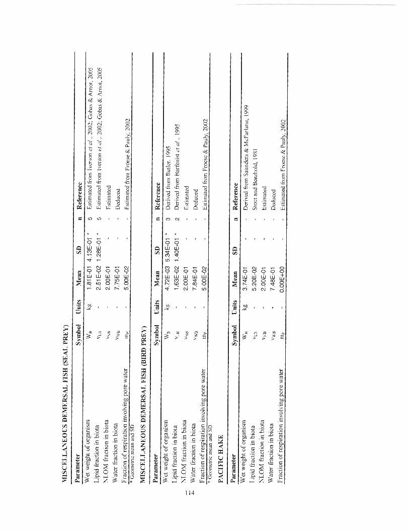
MIS
CE
LL
AN
EO
US
DE
ME
RSA
L F
ISH
(SE
AL
PR
EY
)
Para
met
er
Sym
bol
Uni
ts
Mea
n SD
n
Ref
eren
ce
Wet
wei
ght o
f org
anis
m
*B
kg
1.81
E-0
1 4.
13E
-01
* 5
Est
imat
ed f
rom
lve
rson
e! a
1 .,
2002
; Gob
as &
Arn
ot, 2
005
Lip
id f
ract
ion
in b
iota
V
LB
-
2.51
E-0
2 1.
28E
-01 '
5 E
stim
ated
fro
m I
vers
on e
l 01
.. 20
02;
Gob
as &
Arn
ot, 2
005
NL
OM
fra
ctio
n in
bio
ta
Wat
er f
ract
ion
in b
iota
\'*
B -
2.00
E-0
1 -
Est
imat
ed
v WB
-
7.75
E-0
1 -
Ded
uced
Frac
tion
of re
spir
atio
n in
volv
ing
pore
wat
er
m P
- 5.
00E
-02
- E
stim
ated
fro
m F
roes
e &
Pau
ly, 2
002
* Geo
met
ric m
an
and
SD
MIS
CE
LL
AN
EO
US
DE
lME
RSA
L F
ISH
(B
IRD
PR
EY
)
Para
met
er
Sym
bol
Uni
ts
Mea
n SD
n
Ref
eren
ce
Wet
wei
ght o
f org
anis
m
WB
kg
4.
72E
-03
5.34
E-0
1 '
3 D
eriv
ed f
rom
But
lcr,
1995
Lip
id f
ract
ion
in b
iota
~
LB
-
1.63
E-0
2 1.
40E
-01
" 2
Der
ived
from
Har
feni
st e
r a1 .,
1995
NL
OM
fra
ctio
n in
bio
ta
% B
- 2.
00E
-01
- E
stim
ated
u
P
Wat
er f
ract
ion
in b
iota
','WE
- 7.
84E
-01
- D
educ
ed
Frac
tion
of re
spir
atio
n in
volv
ing
pore
wat
er
m P
- 5.
00E
-02
- E
stim
ated
from
Fro
esc &
Pau
ly, 2
002
* Geo
met
ric m
ean
and
SD
PAC
IFIC
HA
KE
Para
met
er
Sym
bol
Uni
ts
Mea
n SD
n
Ref
eren
ce
Wet
wei
ght o
f or
gani
sm
w B
kg
3.74
E-0
1 -
Der
ived
from
Sau
nder
s &
McF
arla
n e,
1999
Lip
id f
ract
ion
in b
iota
V
LB
-
5.20
E-0
2 -
Stou
t and
Bee
zhol
d, 1
951
NL
OM
fra
ctio
n in
bio
ta
VNB
- 2.
00E
-01
- E
stim
ated
Wat
er f
ract
ion
in b
iota
\'W
B
- 7.
48E
-01
- D
educ
ed
Frac
tion
of r
espi
ratio
n in
volv
ing
pore
wat
er
m P
-
0.00
E+0
0 -
Est
imat
ed f
rom
Fro
esc
& P
auly
, 200
2

SPIN
Y D
OG
FIS
H
Para
met
er
Sym
bol
Uni
ts
Mea
n SD
n
Ref
eren
ce
Wet
wei
ght o
f org
anis
m
WB
kg
2.
00E
+00
2.
00E
-01
9 M
acki
ntos
h et a
/. , 2
004
Lip
id f
ract
ion
in b
iota
"I
LB
- 1.
00E
-01
5.00
E-0
2 9
Mac
kint
osh ei u
l.,
2004
NL
OM
fra
ctio
n in
biot
a V
YB
-
2.00
E-0
1 -
Est
imat
ed
Wat
er f
ract
ion
in b
iota
~
\V
R
- 7.0
0E
-01
- D
educ
ed
Frac
tion
of r
espi
ratio
n in
volv
ing
pore
wat
er
mp
- 0.
00E
+00
-
Est
imat
ed f
rom
Fro
ese
B P
auly
, 300
2
PO
LL
OC
K
Para
met
er
Sym
bol
Uni
ts
Mea
n SD
n
Ref
eren
ce
Wet
wei
ght o
f or
gani
sm
W B
kg
7.97
E-0
2 1 .I 9E
-02
7
Der
ived
from
Iver
son
et a
l., 2
002
Lip
id f
ract
ion
in b
iota
V
LB
- 2.
16E
-02
1.75
E-0
1 '
36
Dcr
ived
fro
m I
vers
on c
t a].,
200
2
- N
LO
M f
ract
ion
in b
iota
V
~B
-
2.00
E-0
1 -
Est
imat
ed
- rn
Wat
er f
ract
ion
in b
iota
V
ii,
- 7.7
8E
-01
- D
educ
ed
Frac
tion
of r
espi
ratio
n in
volv
ing
pore
wat
er
mp
- 0.
00E
+00
- E
stim
ated
fro
m F
roes
e &
Pau
ly, 2
002
" Geo
met
ric
mea
n an
d SD
NO
RT
HE
RN
SM
OO
TH
-TO
NG
UE
Para
met
er
Sym
bol
Uni
ts
Mea
n SD
n
Ref
eren
ce
Wet
wei
ght o
f org
anis
m
W B
kg
7.50
E-0
4 -
Est
imat
ed f
rom
Fro
ese &
Pau
ly, 2
002
Lip
id f
ract
ion
in b
iota
V
LB
-
4.99
E-0
2 -
Est
imat
ed
NL
OM
fra
ctio
n in
bio
ta
%B
-
2.00
E-0
1 -
Est
imat
ed
Wat
er f
ract
ion
in b
iota
~
'\w
-
7.50
E-0
1 -
Ded
uced
Frac
tion
of r
espi
ratio
n in
volv
ing
pore
wat
er
mp
- 0.
00E
+00
-
Est
imat
ed f
rom
Fro
ese 8: P
auly
, 200
2

EN
GL
ISH
SO
LE
Para
met
er
Sym
bol
Uni
ts
Mea
n SD
n
Ref
eren
ce
Wet
wei
ght o
f or
gani
sm
Ws
kg
7.40E-02
- m
acki
ntos
h el
al.,
200
4
Lip
id f
ract
ion
in b
iota
V
LB
-
4.00E-02
- St
out a
nd B
cezh
old,
198
I
NL
OM
fra
ctio
n in
bio
ta
VX
B
- 2.00E-01
- Es
timal
ed
Wat
er f
ract
ion
in b
iota
v
w
- 7.50E-C:
- D
educ
ed
Frac
tion
of r
espi
ratio
n in
volv
ing
pore
wat
er
I~
P
- 5.00E-02
- E
sri~
nate
d from
Fro
ese
& P
auly
, 200
2

Table 6-14 Double-crested Cormorant paranleter definitions, values, aud references
DOUBLE-CRESTED CORMORANT (ADULT MALE)
Parameter Symbol Units ~Mcan SD n Reference Wet weight o f organism Wa kg 2.50E+00 3.50E-01 - G o h s & Arnot, 2005 Lipid fraction in biota VI B 7.50E-02 1.50E-02 - Gobas & Amot, 2005
NLOM fraction in biota VN R 2.00E-01 - Gobas & Arnol, 2005 Water fraction in biota VWD 7.25E-01 - Deduced
Rate of PCB loss via growth kc d-' 0.00E+00 - Estimated Activity Factor AF 3.00E+00 - Gobas & Amot, 2005
GD constant A GDA 3.00E-01 - Gobas & Amot, 2005
DOUBLE-CRESTED CORMORANT (ADULT FEIMALE)
Parameter Symbol Units Mean SD n Reference Wct weight of organism WD kg 2.40E+00 3.50E-01 - Gobas & Arnot, 2005 Lipid fraction in biota VLB 7.50E-02 1.50E-02 - Gobas & Arnot. 2005 NLOM fraction in biota VN B 2.00E-01 - G o b s & Arnot. 2005 Water fraction in biota V\\ R 7.25E-01 - Deduced Rate of PCB loss via growth kc; d.' 0.00E+00 - Esti~nated Activity Factor AF 3.00E+00 - G o h s & Arnot, 2005 G, constant A GDA 3.00E-01 - Gobas & Arnot, 2005
DOUBLE-CRESTED CORMORANT (EGG)
Parameter Symbol Units Mean SD s Reference No. clutches pcr year NCY cluUy~ 1.00E+00 - G o h s & Arnot, 2005 No. eggs pcr clutch NEC cggs 4.00E+00 - G o h s & Arnot, 2005
Wet wcight of egg WE k_9 4.49E-02 - Gobas 8: Arnot, 2005
Lipid content of cgg VLC 4.62E-02 7.00E-02 * 7 Derived fiom Ellio~t er (11. .2005
NLOM contcnt o f c g g V~~ 1.15E-01 - Deduced
Watcr contmt of egg V\VE 8.39E-01 1.08E-03 ' 3 Derivcd tiom Elliott er a/. ,2005

Table 6-15 Great Blue Heron parameter definitions, values, and references
GREAT BLUE HERON (ADULT MALE) ~ - - - - - - - ~ - - - - - - p - p p p - - p p - p p p p - p p - - -
Parameter Symbol Units mean SD n Reference Wct weight o f organis~n WB kg 2.58E+00 2.99E-01 17 Dunning, 1993 Lipid fraction in biota VI 11 7.50E-02 - Eslimatcd
NLOM fraction in biota VN 11 2.00E-01 - Estimated Watcr fraction in biota \ IN u 7.25E-01 - D d u c t d
Ratc o f PCB loss via growth kc d-' 0.00E+00 - Estimated
Activity Factor AF 3.00E+00 - Estitnated GD constant A %A 3.00E-01 - G o h s & Arnot, 2005
GREAT BLUE HERON (ADULT FEMALE)
Parameter Syn~bol Units Mean SD n Reference Wet weight of organism w n kg 2.20E+00 3.37E-01 15 Dunning. 1993 Lipid tkiction in biota V ~ . ~ 7.50E-02 - Estimated
NLOiM fraclion in biota "NU 2.00E-01 - Eslimnted
Water fraction in biota V\\,B 7.25E-01 - Deduccd
Rate o f PCB loss via g o w t h krj d ' 0.00E+00 - Estimated Activity Factor AF 3.00E+00 - Esti~natcd
GD constant A GDA 3.00E-01 - Gobas & Arnot, 2005
GREAT BLUE HERON (EGG)
Parameter Symbol Units Meau SD n Reference No. clutches pcr year NCY clut/yl' 1.00E+00 - Butler, 1995
No. cggs per clutch N EC eggs 4.00E+00 - Butler. 1995 Wct wcight o f egg W ,, kg 7.1 0E-02 - Hcron Working Group, 200 1
Lipid content o f cgg VI.E 6.28E-02 3.01 E-02 ' 12 Derived fi.o~n Ellio~t ef a/. , 2005 NLOIM content of egg V N E 1.20E-01 - Deduccd Watcr content o f cgg "\\I 8.17E-01 3.56E-03 ' 11 Dcrired limn Elliott rt id , 2005
* Cieornctnc mean and S1)

Table 6-16 Harbour seal parameter defieitions, values, and references
HARBOUR SEAL (ADULT MALE)
Parameter Symbol Units Mean S D n Reference Wet weight of organisn~ \Vn kg 8.70E+01 6.60E+00 - Bigg.1969
Lipid fraction in biota Vi.0 4.30E-01 - - Gobas & Amot, 2005
NLOM fraction in biota v ~ n 2.00E-01 - - Gobas & Arnot, 2005
Water fraction in biota V\w 3.70E-01 - - Ikdxluc~rl
Ratc of PCB loss via gowth kc d" 7.50E-05 - - G o b s & Arnot, 2005 Activity Factor AF 2.50E+00 - - Gobas & Amot, 2005 CD constant A GDA 7.00E-02 - - G o b s & h n o t , 2005
HARBOUR SEAL (ADULT FEMALE)
Parameter Symbol Units Mean S D n Reference Wet weight of orginism WB kg 6.48E+01 4.40E+00 - Lipid fraction in biota NLOM liactioli in biota Water rraction in biota Rate of PCB loss via gwvth Activity Factor C, constant A Proporrion of population reproducing Wcight of fetus Lipid contcm of fctus NLOM contcnt of fetus Water content ol' fetus Lipid contcnt of milk NLOM contcnt of milk
Bigg. 1969 P. Ross, personal commrrtricnrion
G o b s & Anlo\ 2005 Deduced Gobas & Arnot. 2005 Gobas 8 Arnot, 2005 G o b s Rr Arnot, 2005 P. Ross, prrso~inl cornst:r~~iculio~~
Dcr~vcd tiom C'ottrrll el a/. , 2002
G o b s & Arnot. 2005 Gobas Rr Arnot, 2005 Dcduccd Esti~natcd lion) Lung et a/. , 2005
Deduced Water contcnt of milk vw\l 3.90E-01 4.29E-02 5 Estimated from L.nng et 01. ,2005
HARBOUR SEAL (1-YEAR OLD)
Parameter Symbol Units Mean S D n Reference Wet weight of organism \vn kg 3.33E+01 2.86E+00 5 Muelkrt era / . , 2003
Lipid fraction in biota v~t3 1.16E-01 - - Muelbert et 01. , 2003
NLOM fraction in biota VNB 2.46E-01 - - Deducod
Watcr fraction in biota V\\B 6.38E-01 - - Muelbert rt nl. , 2003
Ratc of PCB loss via gowtli k~ d-' 1.00E-03 - - Gobas R: Arnot, 2005
Activity Factor AF 2.50E+00 - - G o b s & Arnot, 2005 G, constant A GDA 8.00E-02 - - G o b s & Arnot, 2005
HARBOUR SEAL (PUP)
Parameter Symbol Units Mean SD n Reference
Wct wcight of organism W A kg 2.39E+Ol 5.66E+00 10 Data provldcd by 1% Ross. Lipid liaction in biota \'I 13 4.13E-01 - - Derivcd from bluelbert el u1. ,2003
NLOM tiaction in biota VNO 1.51 E-01 - - D c d u d
Water fraction in biota V\\ 8 4.36E-01 - - Derived kom Muelbert et 01. , 2003
Rate of PCB loss via gowlh kc d-' 2.50E-02 - - Gobas& Arnot.20O.i
Activity Factor t\r: 1.50E+00 - - Gobas (lr Arnot. 2005 GD constant A (LA 6.00E-02 - - Gobas & A~mot, 2005

6.5 Model Sensitivity Analysis
Model sensitivity analysis measures the sensitivity of model predictions to small changes
in individual model parameter values. To test the sensitivity of the SoG bioaccumulation
model to changes in the values of its parameters, I increased individual parameter values,
one at a time, by 1 %, ran the model, and compared the resulting BSAF for a given
organism to that obtained using baseline parameters with the following equation:
S = (BSAFo' - BSAFo) / BSAFo [58I
Where S (unitless) is the model sensitivity; BSAFo7 (nghg) is the BSAF for an organism
calculated after one parameter value is increased by 1 %; and BSAFo (ng/ng) is the BSAF
for an organism calculated using baseline parameter values.
The results of the sensitivity analyses are presented in Figure 6-1 to Figure 6-4. Refer to
the legend in Table 6-1 7 for figure definitions. Note that all parameters were included in
the sensitivity analysis, but, for the sake of brevity, only those with sensitivity values
greater than 0.002 or less than -0.002 are included in the figures below.

Table 6-17
Symbol
12
17
F2
F3 F5
F6
F10 62 84
S1
S2 S4
Organism legend for sensitivity analysis fig~ires
Organism Neocalanus plumchrus
Carnivorous zooplankton
Small pelagic fish (seal prey)
Small pelagic fish (bird prey) Miscellaneous demersal fish (seal prey) Miscellaneous demersal fish (bird prey) Pacific hake
Cormorant (adult female) Heron (adult female)
Seal (adult male) Seal (adult female)
Seal (PUP) -

Figure 6-1 Results of sensitivity analysis for seal pups
F i g ~ ~ r e 6-2 Results of sensitivity analysis for adult male seals
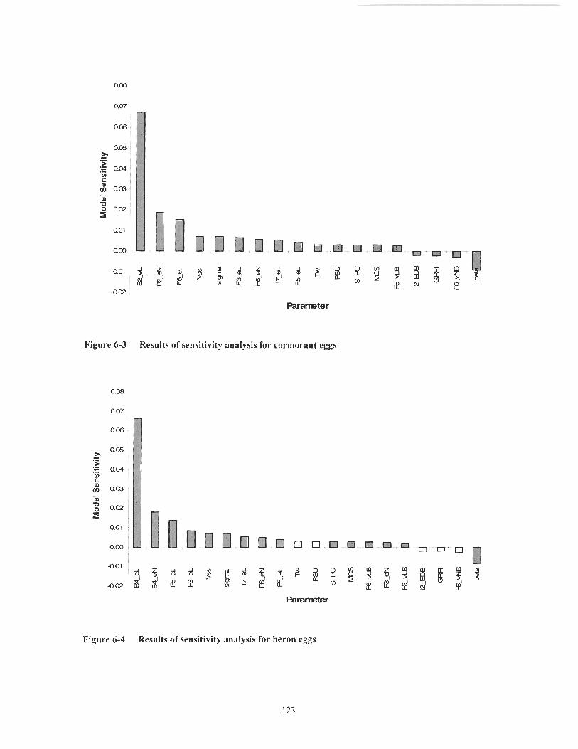
Figure 6-3 Results of sensitivity arlalysis for cormorant eggs
Figure 6-4 Results of sensitivity analysis for heron eggs
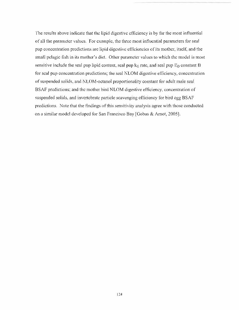
The results above indicate that the lipid digestive efficiency is by far the most influential
of all the parameter values. For example, the three most influential parameters for seal
pup concentration predictions are lipid digestive efficiencies of its mother, itself, and the
small pelagic fish in its mother's diet. Other parameter values to which the model is most
sensitive include the seal pup lipid content, seal pup kc rate, and seal pup ED constant B
for seal pup concentration predictions; the seal NLOM digestive efficiency, concentration
of suspended solids, and NLOM-octanol proportionality constant for adult male seal
BSAF predictions; and the mother bird NLOM digestive efficiency, concentration of
suspended solids, and invertebrate particle scavenging efficiency for bird egg BSAF
predictions. Note that the findings of this sensitivity analysis agree with those conducted
on a similar model developed for San Francisco Bay [Gobas & Amot, 20051.

6.6 Model Performance Analysis Data
Table 6-18 Empirical bird data used to verify model predictions
PCB Congener
I 1 v
Units -- -- 8
15
18/30
28
37
44
49
52
66
74
99 9011 01
105
110
118
128
12911 30
146
149
151
153
156
170
177
180
183J185
187
194
1W199
2031 96
206 209 -
" = not available
CORN Geometric
mean ng/g lipid
2.96E+01
1.71 E+02
1.77E+02
6.42E+02
4.75€+01
2.77E+02
1.05€+03
2.06E+02
1.67€+03
2.81 E+02
6.95E+01
2.65E+02
2.55E+03
1.62€+02
3.80E+02
9,15E+02
2.40E+02
2.37€+02
1.66E+02
1.22E+02
4.31 E+02
Reference: data suppl~ed by Dr. John Ellion
RANT EGG
Log Geomean
1.47
2.23
2.25
2.81
1.68
2.44
3.02
2.31
3.22
2.45
1.84
2.42
3.4 1
2.21
2.58
2.96
2.38
2.37
2.22
2.09
2.63
n = 19)
Geometric SD
ndg lipid
3.12E-01
2.63E-01
2.91 E-01
2.43E-01
2.77E-01
2.54E-01
2.76E-01
1.78E-01
2.66E-01
2.16E-01
2.72E-01
2.68E-01
2.32E-01
2.24E-01
3.08E-01
2.97E-01
2.81E-01
2.21 E-01
3.26E-01
2.58E-01
7.54E-01
HERON EGG (n = 12)
I-- Geometric mean ndg lipid
4.25E+01
2.21 E+02
1.94Ec02
5.74Et02
2.69E+Ol
2.57E+02
1.22E+03
2.42E+02
1.49E+03
1.73E+02
6.1 7E+OO
1.27E+03
1.95E+03
3.72E+02
8.53E+02
2.33E+02
1.29E+02
1.39E+02
4.99E+Ol
LOR Geomean ng/g lipid
1.63
2.34
2.29
2.76
1.43
2.41
3.09
2.38
3.17
2.24
0.79
3.10
3.29
2.57
2.93
2.37
2.11
2.14
1.70
Geometric SD
ndg lipid
8.69E-01
8.88E-01
8.45E-01
4.90E-01
7.09E-01
5.31 E-01
4.68E-01
4.25E-01
4.01E-01
5.76E-01
9.61 E-01
4.63E-01
3.59E-01
3.89E-01
3.46E-01
3.70E-01
4.12E-01
3.75E-01
4.71E-01
Years collected: Cormorant eggs = 1994 & 1995: Heron eggs = 1994 to 2000

Table 6-19 Empirical seal data used to verify model predictions
PCB Congene,
I 1 v
Geometric mean
ndg lipid
1.90E-01
8.29E-02
5.28E-01
6.91 E+00
9.31E-02
1.62E+01
1.12E+01
3.67E+01
4.24E+00
2.02E+01
1.12E+02
9.05E+01
2.06E+01
2.1 1 E+01
5.09E+01
3.35E+01
3.04E+02
6.34E+01
5.35E+01
2.40E+01
3.96E+02
1.76E+01
7.26E+01
3.09E+01
2.1 1 E+02
6.64E+01
1.78E+02
5.05E+01
5.68E+Ol
4.13E+01
1.80E+01 5.48E+00
"-" = not available
-
Reference: data supplied by Dr. Peter Ross
Year collected: 2001
6.7 CD Copy of the Model
ADULT - - -
4
Log Geomean nglg lipid
-0.72
-1.08
-0.28
0.84
-1.03
1.21
1.05
1.56
0.63
1.30
2.05
1.96
1.31
1.32
1.71
1.52
2.48
1.80
1.73
1.38
2.60
1 .25
1.86
1.49
2.32
1.82
2.25
1.70
1.75
1.62
1.26 0.74
SD ndg lipid
1.03E-01
4.55E-02
1.67E-01
9.56E-02
1.07E-01
1.53E-01
1.08E-01
1.65E-01
4.24E-02
1.31 E-01
1.97E-01
1.68E-01
1.40E-01
5.94E-02
1.44E-01
2.09E-01
2.04E-01
2.09E-01
1.38E-01
1.58E-01
2.16E-01
2.03E-01
2.30E-01
1.47E-01
2.43E-01
2.30E-01
2.16E-01
2.76E-01
2.43E-01
2.71 E-01
3.1 3E-01 3.6OE-01
FEMALE SEAL SEAL PUP (n = 10) (n = 4)
Geometric
-- --
Geomean ngg lipid ndg lipid
Please find attached a CD containing an electronic copy of the food web bioaccumulation
model for PCBs described in this document. Microsoft Excel software with enabled
Visual Basic will be required to run the model. The file size is approximately 5 MB.
Instructions for use of the model are located in the model's first worksheet.

REFERENCES
Arnot JA, Gobas FAPC. 2004. A food web bioaccumulation model for organic chemicals in aquatic ecosystems. Environmental Toxicology and Chemistry 23(10): 2343-2355
Arnot JA, Gobas FAPC. 2003. A generic QSAR for assessing the bioaccumulation potential of organic chemicals in aquatic food webs. QSAR and Combinatorial Science 22(3): 337-345.
BC Ministry of Environment. 2006. British Columbia approved water quality guidelines. http://www.env.gov.bc.ca/wat/wq/BCguidelines/ approv~wq_guide/approved.html. Accessed October 21, 2006.
BC Ministry of Environment. 2001. Conservation data centre. http://www.env.gov.bc.ca/cdc/access.html. Accessed October 25, 2006.
Beamish RJ, McFarlane GA, Neville CM, Pearsall I. 2001 a. Changes in the Strait of Georgia ECOPATH model needed to balance the abrupt increases in productivity that occurred in 2000, Bass workshop on the development of a conceptual model of the Subarctic Pacific basin ecosystems. PICES Scientific Report 17, 5-9
Beamish RJ. 1980. Adult biology of the River Lamprey (Lampetra ayresi) and the Pacific Lamprey (Lampetra tridentata) from the Pacific Coast of Canada. Canadian Journal of Fisheries and Aquatic Sciences 37(11): 1906- 1923
Bigg MA. 1969b. The harbour seal in British Columbia. Fisheries research board of Canada 172: 1-33
Boon JP, Oostingh I, Vandermeer J, Hillebrand IMTJ. 1994. A model for the bioaccumulation of chlorobiphenyl congeners in marine mammals. European Journal of Pharmacology - Environmental Toxicology and Pharmacology Section 270(2-3): 237-25 1
Boon JP, Reijnders PJH, Dols J, Wensvooi-t P, Hillebrand MTJ. 1987. The kinetics of individual polychlorinated biphenyl congeners in female harbour seals (Phoca vitulina), with evidence for structure-related metabolism. Aquatic Toxicology 1 O(5-6): 307-324
Boon JP, Vandermeer J, Allchin CR, Law RJ, Klunsoyr J, Leonards PEG, Spliid H, StorrHansen E, Mckenzie C, Wells DE. 1997. Concentration-dependent changes of PCB patterns in fish-eating mammals: Structural evidence for induction of cytochrome P450. Archives of Environmental Contamination and Toxicology 33(3): 298-3 1 1
Burreau S, Zebuhr Y, Broman D, Ishaq R. 2004. Biomagnification of polychlorinated biphenyls (PCBs) and polybrominated diphenyl ethers (PBDEs) studied in pike (Esox lucius), perch (Perca fluviatilis) and roach (Rutilus rutilus) from the Baltic Sea. Chemosphere 55(7): 1043- 1052
Butler RW. 1995. The patient predator: foraging and population ecology of the Great Blue Heron in British Columbia. Canadian Wildlife Service Occasional Paper Number 86, Ottawa, ON, Canada, 44 pp.
Campfens J, Mackay D. 1997. Fugacity-based model of PCB bioaccumulation in complex aquatic food webs. Environmental Science and Technology 3 1: 577-583
Chen JW, Harner T, Schramm KW, Quan X, Xue XY, Kettrup A. 2003. Quantitative relationships between molecular structures, environmental temperatures and octanol-air partition coefticients of polychlorinated biphenyls. Computational Biology and Chemistry 27: 405-42 1
Cohen JE, Pimm SL, Yodzis P, Saldana J. 1993. Body sizes of animal predators and animal prey in food webs. Journal of Animal Ecology 62(1): 67-78
Cottrell PE. 1996. Diet, activity budgets, and movement patterns of harbour seals (Phoca vitulina) in Cowichan Bay and adjacent areas. M.Sc. thesis, University of Victoria, Victoria, BC. 1 18 pp.
Cullon DL, Jeffries SJ, Ross PS. 2005. Persistent organic pollutants in the diet of harbour seals (Phoca vitulina) inhabiting Puget Sound, Washington (USA), and the Striat of Georgia, British Columbia (Canada): a food basket approach. Environmental Toxicology and Chemistry 24( 10): 2562-2572
Davenne E, Masson D. 2001. Water properties in the Straits of Georgia and Juan de Fuca. Fisheries and Oceans Canada report (Institute of Ocean Sciences, Sidney, BC)
deBruyn AMH, Gobas FAPC. Modelling the diagenic fate of persistent organic pollutants in organically enriched sediments. Ecological Modelling 179(3): 405- 416
Deswart RL, Harder TC, Ross PS, Vos HW, Osterhaus ADME. 1995. Morbilliviruses and morbillivirus diseases of marine mammals. Infectious Agents and Disease - Reviews Issue and Commentary 4(3): 125- 130
Drouillard KG, Fernie KJ, Smits JE, Bortolotti GR, Bird DM, Norstrom RJ. 2001. Bioaccumulation and toxicokinetics of 42 polychlorinated biphenyl congeners in American kestrels (Falco spnn~erius). Environmental Toxicology and Chemistry 20(11): 25 14-2522
Drouillard KG, Norstrom RJ. 2000. Dietary absorption efficiencies and toxicokinetics of polychlorinated biphenyls in ring doves following exposure to Aroclor mixtures. Environmental Toxicology and Chemistry 19(11): 2707-27 14
Dunning BD. 1993. CRC handbook of avian body masses. CRC Press Inc. Ann Arbor. ISBN: 0-84'23-4258-9. 71 p.
Elliott JE, Wilson LK, Wakeford B. 2005. Polybrominated Diphenyl Ether Trends in Eggs of Marine and Freshwater Birds from British Columbia, Canada, 1979-2002. Environmental Science and Technology 39: 5584-559 1
Environment Canada. 2004. The toxic substances management policy. http:// www.ec.gc.ca/toxics/en/index.cfin. Accessed December 9, 2004

Environment Canada. 2005. http://www.climate.weatheroffice.ec.gc.cdclimateDatd canada-ehtml. Accessed May 22,2006
Environment Canada. 2005. http://www.pyr.ec.gc.cdgeorgiabasin~basinFacts/ basinFacts-e.htm. Accessed February 1 1,2007
Evanson M, Bornhold EA, Goldblatt RH, Hai-rison PJ, Lewis AG. 2000. Temporal variation in body composition and lipid storage of the overwintering, subarctic copepod Neocalanus plumchrus in the Strait of Georgia, British Columbia (Canada). Marine Ecology Progress Series 192: 239-247
Fisheries and Oceans Canada. 2003. Data from BC Lighthouses. http://www- sci.pac.dfo-mpo.gc.cdosap/datdSearchTools/Searchlighthousee.htm. Accessed 22 May, 2006.
Fisk AT, Hobson KA, Norstrom RJ. 2001. Influence of chemical and biological factors on trophic transfer of persistent organic pollutants in the Northwater Polynya marine food web. Environmental Science and Technology 35(4): 732-738
Froese R, Pauly D. Editors. 2002. FishBase online publication. www.fishbase.org. Accessed March 22, 2006.
Fry B. 1988. Food web structure on Georges Bank from stable C, N, and S isotopic compositions. Limnology and Oceanography 33(5): 1 182- 1 190
Gobas FAPC, Arnot JA. 2005. San Francisco Bay PCB food web model. Prepared for the Clean Estuary Partnership, Oakland, CA.
Gobas FAPC, MacLean LG. 2003. Sediment-water distribution of organic contaminants in aquatic ecosystems: The role of organic carbon mineralization. Environmental Science and Technology 37: 735-74 1
Gobas, FAPC, Morrison HA. 2000. Bioconcentration and biomagnification in the aquatic environment. Handbook of Property Estimation Methods for Chemicals: Environmental and Health Sciences. Eds. R.S. Boethling and D. MacKay. Boca Raton, Lewis Publishers.
Gobas FAPC, Pasternak JP, Lien K, Duncan RK. 1998. Development and field validation of a multimedia exposure assessment model for waste load allocation in aquatic ecosystems: Application to 2,3,7,8-tetrachlorordibenzo-p-dioxin and 2,3,7,8-tetrachlorordibenzofuran in the Fraser River Watershed. Environmental Science and Technology 32: 2442-2449
Gobas FAPC, Wilcockson JB, Russel RW, Haffner GD. 1999. Mechanisms of biomagnification in fish under laboratory and field conditions. Environmental Science and Technology 33: 133-14 1
Hamilton CM, Hites RA, Schwager SJ, Foran JA, Knuth BA, Carpenter DO. 2005. Lipid composition and contaminants in farmed and wild salmon. Environmental Science and Technology 39: 8622-8629
Harfenist A, Whitehead PE, Cretney WJ, Elliot JE. 1995. Food chain sources of polychlorinated dioxins and furans to Great Blue Herons (Ardea herodias)

foraging in the Fraser River Estuary, British Columbia. Canadian Wildlife Service. Technical report series no. 169, 1-26
Harris ML, Elliott JE, Butler RW, Wilson LK. 2003. Reproductive success and chlorinated hydrocarbon contamination of resident great blue herons (Ardea herodias) from coastal British Columbia, Canada, 1977 to 2000. Environmental Pollution 12 1 : 207-227
Harris ML, Wilson LK, Elliott JE. 2005. An assessment of PCBs and OC pesticides in eggs of double-crested (Phalacrocorax auritus) and Pelagic (P. pelagicus) connorants from the west coast of Canada, 1970 to 2002. Ecotoxicology 14: 607- 62 5
Harrison PJ, Fulton JD, Taylor FJR, Parsons TR. 1983. Review of the biological oceanography of the Strait of Georgia pelagic environment. Canadian Journal of Fisheries and Aquatic Sciences 40(7): 1064- 1094
Heath WA. 1977. The ecology and harvesting of euphausiids in the Strait of Georgia. Ph.D. Thesis, University of British Columbia, 187p.
Hebert CE, Weseloh DVC. 2006. Adjusting for temporal change in trophic position results in reduced rates of contaminant decline. Environmental Science and Technology 40: 5624-5628
Heron Working Group (SFU). 2001. http:l/www.sfu.ca~biology/wildber~wg! aboutherons.htm1. Accessed 22 March, 2006.
Hirons AC, Schell DM, Finney BP. 2001. Temporal records of 6-13C and delta 6-15N in North Pacific pinnipeds: inference regarding environmental change and diet. Oecologia 129(4): 59 1-60 1
Hites RA, Foran JA, Carpenter DO, Hamilton MC, Knuth BA, Schwager SJ. 2004. Global assessment of organic contaminants in farmed salmon. Science 303(5655): 226-229
Hobson KA, Piatt JF, Pitocchelli J. 1994. Using stable isotopes to determine seabird trophic relationships. Journal of Animal Ecology 63(4): 786-798
Hoffman DJ, Rice CP, Kubiak TJ. 1996. PCBs and dioxins in birds. In "Environmental Contaminants in Wildlife: Interpreting Tissue Concentrations" Eds. Beyer WN, Heinz GH, and Redmon-Nonvood AW. 165-207
Huntley ME, Zhou M. 2004. Influence of animals on turbulence in the sea. Marine Ecology-Progress Series 273: 65-79
Ikonomou MG, Fernandez MP, Knapp W, Sather P. 2002. PCBs in Dungeness Crab Reflect Distinct Source Fingerprints among Harbor/Industrial Sites in British Columbia. Environmental Science and Techology 36 (1 2): 2545-2 55 1
Iverson SJ, Frost KJ, Lang SLC. 2002. Fat content and fatty acid composition of forage fish and invertebrates in Prince William Sound, Alaska: factors contributing to among and within species variability. Marine Ecology Progress Series 24 1 : 16 1 - 181
Jeffries S, Huber H, Calambokidis J, Laake J. 2003. Trends and status of harbor seals in Washington State: 1978 - 1999. Journal of Wildlife Management 67(1): 208-2 19
Jennings S, Pinnegar JK, Polunin NVC, Boon TW. 2001. Weak cross-species relationships between body size and trophic level belie powerful size-based trophic structuring in fish communities. Journal of Animal Ecology 70(6): 934- 944
Johannessen SC, Macdonald RW, Paton DW. 2003. A sediment and organic carbon budget for the greater Strait of Georgia. Estuarine, Coastal and Shelf Science 56: 845-860
Kannan K, Blankenship AL, Jones PD, Giesy JP. 2000. Toxicity reference values for the toxic effects of polychlorinated biphenyls to aquatic mammals. Human and Ecological Risk Assessment 6(1): 18 1-20 1
Kelly BC, Gobas FAPC. 2001. Bioaccumulation of persistent organic pollutants in lichen-caribou-wolf food chains of Canada's Central and Western Arctic. Environmental Science and Technology 35(2): 325-334
Kelly BC, Gobas FAPC, McLachlan MS. 2004. Intestinal absorption and biomagnification of organic contaminants in fish, wildlife, and humans. Environmental Toxicology and Chemistry 23 (1 0): 2324-233 6
Lang SLC, Iverson SJ, Bowen WD. 2005. Individual variation in milk composition over lactation in harbour seals (Phoca vitulina) and the potential consequences of intermittent attendance. Canadian Journal of Zoology 83: 1525-1 53 1
Larsen LO. 1980. Physiology of adult lampreys, with special regard to natural starvation, reproduction, and death after spawning. Canadian Journal of Fisheries and Aquatic Sciences 37(11): 1762- 1779
Lassuy DR. 1989. Species profiles: life history and environmental requirements of coastal fishes and invertebrates (Pacific Northwest) - Pacific Herring. US Fish and Wildlife Service Biological Report 82(11.126). US Army Corps of Engineers, TR-EL-82-4. 18pp.
Lee RF. 1974. Lipids of zooplankton from Bute Inlet, BC. Journal of the Fisheries research board of Canada 3 1 : 1577- 1582
Li N, Wania F, Lei YD, Daly GL. 2003. A comprehensive and critical compilation, evaluation, and selection of physical-chemical property data for selected polychlorinated biphenyls. Journal of Physical and Chemical Reference Data 32(4): 1545- 1590
Mackay D. 1991. Multimedia Environmental Models: The Fugacity Approach. Boca Raton, CRC PressILewis Publishers.
Mackintosh CE, Maldonado J, Hongwu J, Hoover N, Chong A, Ikonomou MG, Gobas FAPC. 2004. Distribution of phthalate esters in a marine aquatic food web: comparison to polychlorinated biphenyls. Environmental Science and Technology 38: 201 1-2020
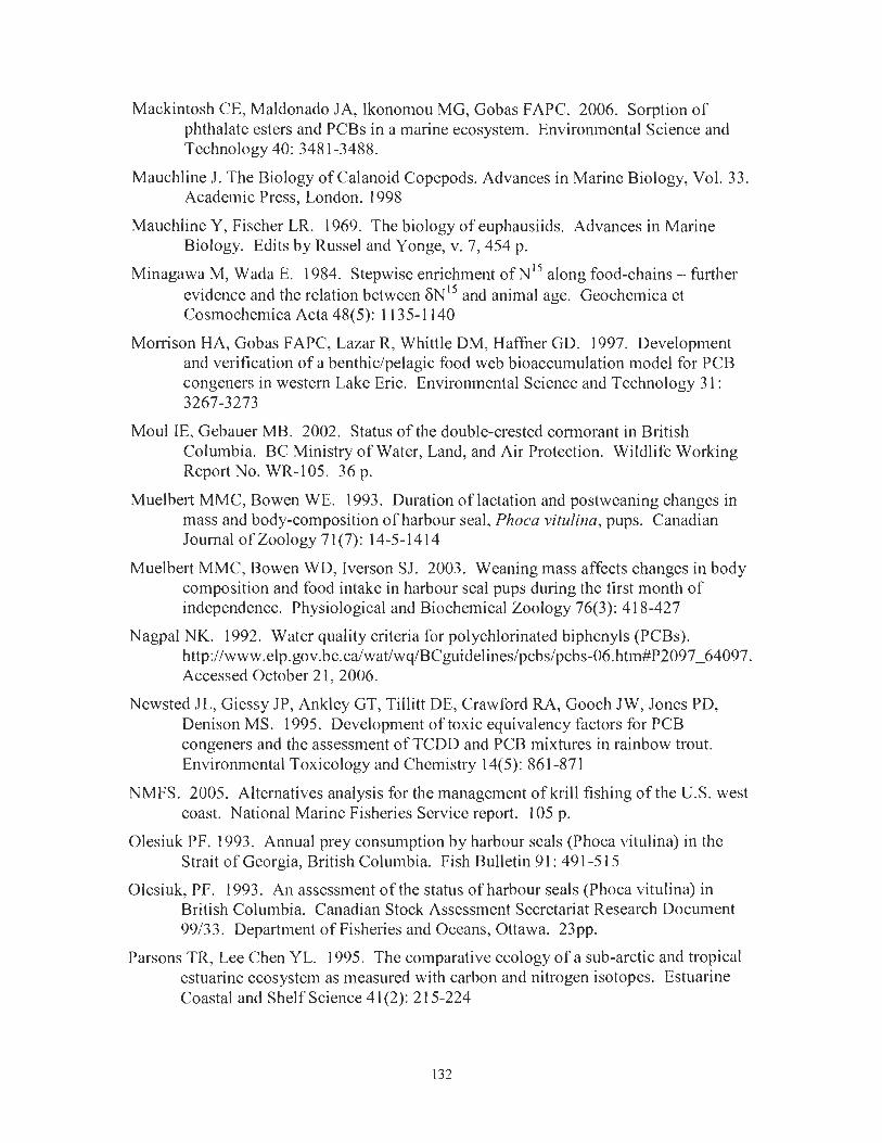
Mackintosh CE, Maldonado JA, Ikonomou MG, Gobas FAPC. 2006. Sorption of phthalate esters and PCBs in a marine ecosystem. Environmental Science and Technology 40: 348 1-3488.
Mauchline J. The Biology of Calanoid Copepods. Advances in Marine Biology, Vol. 33. Academic Press, London. 1998
Mauchline Y, Fischer LR. 1969. The biology of euphausiids. Advances in Marine Biology. Edits by Russel and Yonge, v. 7,454 p.
Minagawa M, Wada E. 1984. Stepwise enrichment of N" along food-chains - further evidence and the relation between 6 ~ ' ~ and animal age. Geochemica et Cosmocheinica Acta 48(5): 1 135- 1 140
Morrison HA, Gobas FAPC, Lazar R, Whittle DM, Haffner GD. 1997. Development and verification of a benthiclpelagic food web bioaccumulation model for PCB congeners in western Lake Erie. Environmental Science and Technology 3 1 : 3267-3273
Moul IE, Gebauer MB. 2002. Status of the double-crested cormorant in British Columbia. BC Ministry of Water, Land, and Air Protection. Wildlife Working Report No. WR-105. 36 p.
Muelbert MMC, Bowen WE. 1993. Duration of lactation and postweaning changes in mass and body-composition of harbour seal, Phoca vitulina, pups. Canadian Journal of Zoology 7 l(7): 14-5- 14 14
Muelbert MMC, Bowcn WD, Iverson SJ. 2003. Weaning mass affects changes in body composition and food intake in harbour seal pups during the first month of independence. Physiological and Biochemical Zoology 76(3): 4 18-427
Nagpal NK. 1992. Water quality criteria for polychlorinated biphenyls (PCBs). http://www.elp.gov.bc.calwat/wq/BC~idelines/pcbs/pcbs-06. htm#P2097-64097. Accessed October 2 1, 2006.
Newsted JL, Giessy JP, Ankley GT, Tillitt DE, Crawford RA, Gooch JW, Jones PD, Denison MS. 1995. Development of toxic equivalency factors for PCB congeners and the assessment of TCDD and PCB mixtures in rainbow trout. Environmental Toxicology and Chemistry 14(5): 861 -87 1
NMFS. 2005. Alternatives analysis for the management of krill fishing of the U.S. west coast. National Marine Fisheries Service report. 105 p.
Olesiuk PF. 1993. Annual prey consumption by harbour seals (Phoca vitulina) in the Strait of Georgia, British Columbia. Fish Bulletin 91 : 491 -5 15
Olesiuk, PF. 1993. An assessment of the status of harbour seals (Phoca vitulina) in British Columbia. Canadian Stock Assessment Secretariat Research Document 99/33. Department of Fisheries and Oceans, Ottawa. 23pp.
Parsons TR, Lee Chen YL. 1995. The comparative ecology of a sub-arctic and tropical estuarine ecosystem as measured with carbon and nitrogen isotopes. Estuarine Coastal and Shelf Science 4 l(2): 2 15-224

Pauly D, Christensen V, Editors. 1995. Mass-Balance Models of Northeastern Pacific Ecosystems. Proceedings of a Workshop held at the Fisheries Centre, University of British Columbia, Vancouver, Canada, B. C., November 6- 10, 1995; UBC Fisheries Centre Research Reports 4(1): Vancouver, BC, Canada, p 13 1 .
Pawlowicz R, Allen S, Dower J, Lee R, Harris S, Halverson M, Riche 0, Bird T. 2003. Stratagem - The Strait of Georgia Ecosystem Project. Presented at the 2003 Georgia Basin / Puget Sound Research Conference.
Robertson, I. 1974. The food of nesting Double-crested and Pelagic Cormorants at Mandarte Island, British Columbia, with notes on feeding ecology. Condor 76: 346-348.
Ross PS, Ellis GM, Ikonomou MG, Bai~ett-Lennard LG, Addison RF. 2000. High PCB concentrations in free-ranging Pacific killer whales, Orcinus orca: Effects of age, sex and dietary preference. Marine Pollution Bulletin 40(6): 504-5 15
Ross PS, Jeffries SJ, Yunker MB, Addison RF, Ikonomou MG, Calambokidis JC. 2004. Harbor seals (Phoca vitulina) in British Columbia, Canada, and Washington State, USA, reveal a combination of local and global polychlorinated biphenyl, dioxin, and h r a n signals. Environmental Toxicology and Chemistry 23(1): 157- 165
Sample BE, Suter I1 GW. 1994. Estimating exposure of terrestrial wildlife to contaminants. Oak Ridge National Laboratory Report ESIERITM- 125. 49 p.
Sargent JR, Lee RF. 1975. Biosynthesis of Lipids in zooplankton from Saanich Inlet, BC, Canada. Marine Biology 3 1 : 15-23
Saunders MW, McFarlane GA. 1999. Pacific Hake - Strait of Georgia stock assessment for 1999 and recommended yield options for 2000. Canadian Stock Assessment Secretariat Research Document 99/200, ISSN 1480-4883, Ottawa, 1999, 1 1 p.
Sharpe S, Mackay D. 2000. A framework for evaluating bioaccumulation in food webs. Environmental Science and Technology 34( 12): 2373-2379
Stevenson RW. 2003. Development and application of a model describing the bioaccumulation and metabolism of polycyclic aromatic hydrocarbons in a marine benthic food web. MRM Project. SFU, Burnaby, BC.
Stout VF, Beezhold FL. I98 1 . Chlorinated-hydrocarbon levels in fishes and shellfishes of the northeastern pacific-ocean, including the Hawaiian-Islands. Marine Fisheries Review 43(1): 1 - 12
Sullivan TM. 1998. The timing of breeding in Double-crested Cormorants (Phalacrocorax auritus albociliatus): its effects on clutch size, nestling growth, diet and survival. MSc. Thesis. UBC, Vancouver, BC.
Swain LO, Walton DG. 1994. 1993 Survey of Sediments and Tissues from Boundary Bay and Roberts Bank. British Columbia Ministry of Environment, Land and Parks report WQWM 93- 1 2
Thomann RV, Connolly JP, Parkerton TF. 1992. An equilibrium-model of organic- chemical accumulation in aquatic food webs with sediment interaction. Environmental Toxicology and Chemistry 1 l(5): 61 5-629

Trumble SJ, Barboza PS, Castellini MA. 2003. Digestive constraints on an aquatic carnivore: effect of feeding frequency and prey composition on harbor seals. Journal of Comparative Physiology B 173: 501-509
US Environmental Protection Agency. 1992a. Framework for ecological risk assessment. Risk Assessment Forum, Washington, DC. EPAI63OlR-02/011
US Environmental Protection Agency. 1999. Evaluation of toxicity and bioaccumulation of contaminants in sediments samples from Waukegan Harbor, Illinois. EPA-905/R-99/009. US Environmental Protection Agency, Chicago, IL, USA. 28p.
US Environmental Protection Agency. 200 1. The role of screening-level risk assessments and refining contaminants of concern in baseline ecological risk assessments. USEPA Publication 9345.0- 14. 8p.
US Environnlental Protection Agency. 2006. USEPA online terminology reference center. http://www.epa.gov/trs/. Accessed October 29, 2006
Van den Berg M, Birnbaum L, Bosveld AT, Brunstrom B, Cook P, Feeley M, Giesy JP, Hanberg A, Hasegawa R, Kennedy SW, Kubiak T, Larsen JC, van Leeuwen FX, Liem AK, Nolt C, Peterson RE, Poellinger L, Safe S, Schrenk D, Tillitt D, Tysklind M, Younes M, Waern F, Zacharewski T. 1998. Toxic equivalency factors (TEFs) for PCBs, PCDDs, PCDFs for humans and wildlife. Environinental Health Perspectives 106: 775-792.
Vander Zanden MJ, Rasmussen JB. 1996. A trophic position model of pelagic food webs: impact on contaminant bioaccumulation in lake trout. Ecological Monographs 66(4): 45 1-477
Verbeek NAM, Butler RW. 1989. Feeding ecology of shoreline birds in the Strait of Georgia. In: Vermeer, K.; Butler, R.W. (Eds.), The Ecology and Status of Marine and Shoreline Birds in the Strait of Georgia, British Columbia. Canadian Wildlife Service Special Publication, Ottawa, ON, Canada, p. 74
Wania F, Mackay D. 1999. The evolution of mass balance models of persistent organic pollutant fate in the environment. Environmental Pollution 100: 223-240
West J, O'Neill S, Lippert G, Quinnell S. 2001. Toxic contaminants in marine and anadromous fishes from Puget Sound, Washington. Washington Department of Fish and Wildlife, 3 1 1 p.
West JE, O'Neill SM, Ylitalo GM. 2006. Spatial extent, magnitude, and patterns of persistent organic pollutants in Pacific herring (Clupeapallasi) populations; implications for the Puget Sound and Strait of Georgia pelagic food web. http://www.pugetsoundpartnership.org/news/letters/septO6/WestetalHengPOP subn~ittaltoCJFAS.pdf Accessed on October 22,2006.