development of a 3-dof motion simulation platform

Development of a 3-DOF Motion Simulation Platform

by

Philip Ethelbert Smit

Thesis presented in partial fulfilment of the requirements for the degree of

Master of Science in Engineering

at Stellenbosch University

Supervisor: Dr I.K. Peddle

Co-Supervisor: Prof T. Jones

Department of Electrical and Electronic Engineering

March 2010

ii

Declaration

By submitting this thesis electronically, I declare that the entirety of the work contained therein is my own, original work, that I am the owner of the copyright thereof (unless to the extent explicitly otherwise stated) and that I have not previously in its entirety or in part submitted it for obtaining any qualification.

March 2010

Copyright ©2010 Stellenbosch University All rights reserved

iii

Abstract The successful development of a three degree of freedom motion simulation platform, capable of simulating a vessel’s flight deck at sea, is presented. The motion simulation platform was developed to practically simulate and test an unmanned aerial vehicle’s capability of landing on a moving vessel, before practically being demonstrated on an actual vessel. All aspects of the motion simulation platform’s development are considered, from the conceptual design to its practical implementation. The mechanical design and construction of a pneumatic motion simulation platform, as well as the electronics and software to enable the operation of this motion simulation platform, are presented. Mathematical models of the pneumatic process and platform orientation are developed. A controller architecture capable of regulating the pneumatic process, resulted in the successful control of the motion simulation platform. Practical motion simulation results of one of the South African Navy Patrol Corvettes, demonstrate the motion simulation platform’s success. The successful development of the motion simulation platform can largely be attributed to extensive research, planning and evaluation of the different development phases.

iv

Opsomming In hierdie studie word die suksesvolle ontwikkeling van ’n drie-grade-van-vryheid bewegingsimulasieplatform, wat in staat is daartoe om ’n skip se vliegdek ter see te simuleer, aangebied. Die bewegingsimulasieplatform is ontwikkel om ’n onbemande lugvaartuig se vermoë om op ’n bewegende skip te land, te simuleer en te toets, voor dit op ’n werklike skip gedemonstreer word. Alle aspekte van die ontwikkeling van die bewegingsimulasieplatform word in ag geneem – van die konsepontwerp tot die praktiese implementering daarvan. Die meganiese ontwerp en konstruksie van ’n pneumatiese bewegingsimulasieplatform word bespreek, sowel as die elektronika en programmatuur wat die werking van hierdie bewegingsimulasieplatform bemoontlik. Wiskundige modelle van die pneumatiese proses en platformoriëntering word ontwikkel. ’n Beheerderargitektuur wat in staat is daartoe om die pneumatiese proses te reguleer, lei tot die suksesvolle beheer van die bewegingsimulasieplatform. Praktiese resultate van die bewegingsimulering van een van die Suid-Afrikaanse Vloot se patrolliekorvette wys daarop dat die bewegingsimulasieplatform wel suksesvol is. Die geslaagde ontwikkeling van die bewegingsimulasieplatform kan grootliks toegeskryf word aan omvangryke navorsing, beplanning en evaluering van die onderskeie ontwikkelingsfases.

v

Acknowledgements

I would like to express my sincere gratitude to all the people who have contributed to making a project of this magnitude and complexity possible. In particular, I would like to extend my gratitude to.

• Dr I.K. Peddle for your guidance, friendship, advice and willingness to always provide insight and support on many aspects of this project.

• Prof T. Jones for your guidance, support and advice.

• IMT Radar for providing ship motion data of the South African Navy Patrol Corvettes.

• Rudi Gaum for helping me get to terms with numerous theoretical problems and for always being there whenever I required advice.

• Deon Blaauw for your assistance with the electronics developed in this project and for the company on all the late nights spent in the lab.

• Wessel Croukamp and Lincoln Saunders, for their advice, support and immense effort and time in assisting with the mechanical construction of this project.

• All my friends in the ESL for their welcoming advice and assistance during this project.

• My parents and brother for their continued love and support.

vi

Contents

Declaration ii

Abstract iii

Opsomming iv

Acknowledgements v

Contents vi

List of Figures xi

List of Tables xvi

Nomenclature xvii

Chapter 1 – Introduction and Overview 1

1.1 Background 1

1.2 Project Description and Objectives 2

1.3 Thesis Outline 4

Chapter 2 – Conceptual Design 6

2.1 User Requirements and Engineering Specifications 6

2.2 Types of Linear Actuation 8

2.2.1 Electrical System 8

2.2.2 Hydraulic System 9

2.2.3 Pneumatic System 11

vii

2.2.4 Actuator Overview 12

2.3 Concept Generation and Investigation 13

2.3.1 Concept 1 13

2.3.2 Concept 2 15

2.3.3 Concept 3 16

2.3.4 Concept 4 18

2.4 Summary 19

Chapter 3 – Mechanical Design 20

3.1 Functional Analysis Decomposition 20

3.2 Linear Pneumatic Actuator 22

3.2.1 Displacement Sensor 24

3.2.2 Cylinder Support 25

3.3 Simulation Platform 26

3.3.1 Upper Joint (2 DOF) 26

3.4 Base Structure 27

3.4.1 Valve Unit 29

3.5 Main Mechanical System 30

3.6 Mechanical Construction 31

3.7 Summary 32

Chapter 4 – Electronic and Software Design 33

4.1 Electronics 34

4.1.1 Pneumatic Control Electronics Module 34

4.1.2 Bluetooth Module 37

4.2 Computer Software 38

4.2.1 Simulink Interface 39

viii

4.2.2 Motion Simulation Platform GUI 40

4.3 Summary 41

Chapter 5 – Pneumatic Model 42

5.1 Nonlinear Pneumatic Model 42

5.1.1 Valve Model 43

5.1.2 Cylinder Chambers Model 44

5.1.3 Piston-Load Dynamics 47

5.1.4 Model Validation 48

5.2 Simplified Linear Pneumatic Model 49

5.2.1 Model Derivation and Parameter Identification 50

5.2.2 Friction Function 53

5.2.3 Model Validation 56

5.3 Summary 57

Chapter 6 – Pneumatic Control 58

6.1 Description of Experimental Setup 58

6.2 Sliding Mode Control Design 59

6.2.1 Feedback Measurement Filtering 62

6.2.2 Simulation and Practical Results 64

6.3 Friction Function 66

6.4 Reference Monitoring 69

6.5 Evaluation of Practical Results 70

6.5.1 Sinusoidal Tracking 70

6.5.2 Sinusoidal Tracking with Mass 72

6.5.3 Ship Heave Motion Tracking 73

6.6 Summary 73

ix

Chapter 7 – Platform Model and Control 74

7.1 Platform Orientation Model 74

7.1.1 Platform Parameter Definition and Constraint Equations 75

7.1.2 Ship Orientation to Piston Stroke 79

7.1.3 Piston Stroke to Ship Orientation 81

7.1.4 Model Overview 84

7.2 Platform Control 85

7.2.1 Reference Step Response 87

7.2.2 Sinusoidal Tracking 88

7.3 Summary 89

Chapter 8 – Ship Motion Simulation 90

8.1 Record Point Transformation 90

8.2 Ship Motion Processing 92

8.3 Motion Simulation Results 95

8.4 Summary 99

Chapter 9 – Summary and Recommendations 100

9.1 Summary 100

9.2 Recommendations 101

Appendix A – Mechanical Details 104

A.1 Component Cost and Mass Summary 104

A.2 Dimensional Overview 105

A.3 Deflection Calculation 1 106

A.4 Deflection Calculation 2 108

Appendix B – Modelling Parameters 110

x

B.1 Nonlinear Pneumatic Model Parameters 110

B.2 Simplified Linear Pneumatic Model Parameters 111

B.3 Platform Orientation Model Parameters 112

Appendix C – Ship Motion Data 113

C.1 Ship Axis System 113

C.2 Ship Motion Data 114

Bibliography 118

xi

List of Figures

1.1 South African Navy Valour Class Patrol Corvette [24] 2

1.2 Rotary and Fixed-wing Landing Configurations 3

1.3 3-DOF and 6-DOF Motion Simulation Platform [25] 3

1.4 Thesis Outline 4

2.1 Electrical System Overview 9

2.2 Hydraulic System Overview 10

2.3 Pneumatic System Overview 11

2.4 Concept 1 Overview 14




3.1 Functional Analysis Decomposition 21

3.2 Linear Pneumatic Actuator Overview 22

3.3 Linear Pneumatic Actuator 22

3.4 Pneumatic Cylinder 23

3.5 Displacement Sensor 24

3.6 Cylinder Support 25

3.7 Simulation Platform 26

3.8 Upper Joint (2 DOF) 27

3.9 Base Structure 28

xii

3.10 Lower Joint (1 DOF) 28

3.11 Valve Unit 29

3.12 Main Mechanical System (CAD) 30

3.13 Construction of Main Mechanical System 31

4.1 Electronic and Software Overview 33

4.2 Pneumatic Control Electronics Module (left) and Battery Pack (right) 34

4.3 Block Diagram of Pneumatic Controller Board 35

4.4 Top and Bottom Layers of Pneumatic Controller Board 36

4.5 Parani-ESD1000 (left) and Bluetooth Module (right) 38

4.6 Simulink Direct Interface 39

4.7 Simulink Control Interface 39

4.8 Control Page 40

4.9 Platform Monitor Page 41

5.1 Pneumatic Cylinder and Valve Overview 43

5.2 Proportional Directional Control Valve [2] 44

5.3 System Dynamics of the Nonlinear Pneumatic Model 48

5.4 Validation of the Nonlinear Pneumatic Model 49

5.5 Simplified Pneumatic System Overview 50

5.6 Open loop Step Response 52

5.7 Open loop Poles of the Simplified Pneumatic Model 53

5.8 Friction Function Block Diagram 54

5.9 Static Friction Effect 54

5.10 Friction Function Control Input Relation 55

5.11 Validation of the Simplified Linear Pneumatic Model 56

5.12 Nonlinear inaccuracies of the Simplified Linear Pneumatic Model 57

6.1 Experimental Setup 59

xiii

6.2 Saturation Function and Boundary layer 61

6.3 Block Diagram of the Pneumatic Position Control 62

6.4 Closed Loop Poles at ϕ=250 64

6.5 Simulation results of Piston Position Control 65

6.6 Practical Sinusoidal Reference Tracking at 1.2 rad/s 66

6.7 Effective Saturation Function change with Friction Function 67

6.8 Friction Function effects on Sinusoidal Tracking at 1.2 rad/s 67

6.9 Sinusoidal Tracking at 1.2 rad/s with Reference Delay 68

6.10 Reference Monitoring Results 69

6.11 Sinusoidal Tracking with Increasing Amplitude at 0.5 rad/s 71

6.12 Sinusoidal Tracking with Increasing Amplitude at 1.2 rad/s 71

6.13 Sinusoidal Tracking with Increasing Amplitude at 2 rad/s 72

6.14 Sinusoidal Tracking with Increasing in Mass at 1.2 rad/s 72

6.15 Ship Heave Motion Tracking 73

7.1 Ship Orientation 74

7.2 Platform Orientation Model Block Diagram 75

7.3 Platform Orientation 76

7.4 Motion Simulation Platform Constraint Planes 76

7.5 Definition of the Platform Pitch Angle 77

7.6 Piston Stroke versus Ship Orientation 84

7.7 Coupling into Undesired Degrees of Freedom 85

7.8 Platform Control Block Diagram 85

7.9 Heave Reference Step Response 87

7.10 Pitch Reference Step Response 87

7.11 Roll Reference Step Response 87

7.12 Sinusoidal Heave Tracking at 1.2 rad/s 88

xiv

7.13 Sinusoidal Pitch Tracking at 1.2 rad/s 88

7.14 Sinusoidal Roll Tracking at 1.2 rad/s 89

8.1 Record Point Transformation 91

8.2 Frequency Content of the Ship’s Flight Deck Heave Motion 93

8.3 Ship Motion Processing and Heave Filtering 93

8.4 LPF Magnitude and Phase Response 95

8.5 HPF Magnitude and Phase Response 95

8.6 Graphical Simulator 96


8.8 Ship Pitch Motion Tracking 97

8.9 Ship Roll Motion Tracking 97

8.10 Saturation Function 98


A.1 Dimensional Overview 105

A.2 Deflection Calculation 1 Overview 106

A.3 Piston tip deflection 1 108

A.4 Deflection Calculation 2 Overview 108

A.5 Piston tip deflection 2 109

C.1 Ship Axis System 113

C.2 Recording Point Heading 114

C.3 Recording Point Heading Rate 115

C.4 Recording Point Heave 115

C.5 Recording Point Heave Rate 115

C.6 Recording Point Pitch 115

C.7 Recording Point Pitch Rate 116

C.8 Recording Point Roll 116

xv

C.9 Recording Point Roll Rate 116

C.10 Transformed Flight Deck Heave 116

C.11 Transformed Flight Deck Heave Rate 117

xvi

List of Tables

2.1 User Requirements and Engineering Specifications 8

2.2 Actuator Overview 13

3.1 Displacement Sensor Specifications 24

7.1 Control Parameters 86

A.1 Mechanical Component Cost 104

A.2 Mechanical Mass Summary 105

B.1 Nonlinear Pneumatic Model Parameters 111

B.2 Simplified Linear Pneumatic Model Parameters 111

B.3 Platform Orientation Model Parameters 112

C.1 Details of the Ship’s Axis System 114

C.2 Position Offsets 114

xvii

Nomenclature Greek Letters:

β Viscous friction coefficient

ς Damping ratio

θ Platform roll angle

κ Specific heat ratio of air

HPSτ High-pass FIR filter group delay

LPFτ Low-pass FIR filter group delay

Tτ Total group delay

φ Platform pitch angle

ψ Platform yaw angle, Discharge coefficient

nω Natural frequency

Θ Ship pitch angle

RΘ Ship pitch angle reference

RPΘ Recording point pitch angle

Φ Ship roll angle

RΦ Ship roll angle reference

RPΦ Recording point roll angle

Ψ Ship yaw angle Small Letters:

c Damping coefficient

h Platform centre point height

xviii

0h Platform center point offset height

k Spring stiffness

m Mass

m Mass flow rate

Am Mass flow rate to chamber A

Bm Mass flow rate to chamber B

p Platform piston stroke

0p Linear pneumatic actuator offset length

Rp Platform piston stroke reference

r Iteration number

crr Critical pressure ratio

u Control input

valveu Valve input

v Specific volume

vy Control spool movement

x Piston position

x Piston velocity

x Piston acceleration

Rx Piston position reference Capital Letters:

A Piston effective area

AA Piston effective area of chamber A

BA Piston effective area of chamber B

rA Piston rod cross section area

vA Effective area of the valve’s orifice

vC Valve constant

dfF Coulomb friction force

fF Static and Coulomb friction forces

xix

LF External force

sfF Static friction force

H Ship heave

FDH Flight deck heave

FDH Mean flight deck heave

0FDH Flight deck heave about a zero mean

RH Ship heave reference

RPH Recording point heave

iK Valve current gain

vK Velocity gain

M Total system mass

pM Piston rod assembly mass

LM External load mass

P Linear pneumatic actuator total length

aP Atmospheric pressure

AP Pressure in cylinder chamber A

BP Pressure in cylinder chamber B

dP Downstream air pressure

sP Supply pressure

uP Upstream air pressure

R Ideal gas constant

nR Valve solenoid resistance

T Temperature

V Maximum control valve voltage

0V Chamber starting volume

AV Volume of chamber A

BV Volume of chamber B

hiV Upper valve offset

lowV Lower valve offset

TV Total cylinder volume

xx

Acronyms:

2D Two Dimensional

AC Alternating Current

CAD Computer Aided Design

CAN Controller Area Network

DAC Digital to Analogue Converter

DC Direct Current

DFT Discrete Fourier Transform

DOF Degrees of Freedom

FIR Finite Impulse Response

GUI Graphical User Interface

HPF High-Pass Filter

IIR Infinite Impulse Response

IMT Institute for Maritime Technology

IMU Inertial Measurement Unit

INS Inertial Navigation System

LED Light Emitting Diode

LPF Low-Pass Filter

OEM Original Equipment Manufacturer

PC Personal Computer

PWM Pulse Width Modulation

RMS Root Mean Square

SLMC Sliding Mode Control

SPI Serial Peripheral Interface

UART Universal Asynchronous Receiver and Transmitter

UAV Unmanned Aerial Vehicle

USB Universal Serial Bus

1

Chapter 1

Introduction and Overview

1.1 Background

An Unmanned Aerial Vehicle (UAV) can be defined as a powered aerial vehicle that does not carry a human operator and can fly autonomously, using aerodynamic forces to provide vehicle lift [18]. According to a recent market study done by the Teal Group, an aerospace and defence industry market analysis firm based in the United States, UAVs continue to be the most dynamic growth sector of the world aerospace industry [19]. Teal Group's 2009 market study estimates that UAV spending will almost double over the next decade from current worldwide UAV expenditures of $4.4 billion annually to $8.7 billion, totalling just over $62 billion in the next ten years. According to [20], South Africa plays an important role in the development of UAV capabilities, as South Africa can utilise the mostly unoccupied airspace between South Africa and Antarctica for extensive UAV testing. There are many civil as well military applications for UAVs including surveillance, reconnaissance, search and rescue, radio and data relay, law enforcement and fire suppression. The Centre of Expertise (CoX) in Autonomous Systems Group, a subdivision of the Electrical and Electronic Engineering Department at the Stellenbosch University, conducts active research in the field of UAVs. This group has experienced rapid growth in UAV research and has practically demonstrated complete autonomous waypoint navigation of fixed-wing as well as rotary-wing aircraft in multiple projects. Autonomous take-off and landing of a fixed-wing aircraft has also practically been demonstrated. The development of an autonomous take-off and landing autopilot for a rotary-wing aircraft has almost been completed and is expected to be demonstrated in 2010 [21]. In an endeavour to further this research, two projects, [22] and [23], are currently underway to develop and practically test a fixed- and rotary-wing autopilot which is capable of performing an autonomous landing on a moving platform relating to the motion of a ship’s flight deck at sea.

CHAPTER 1 – INTRODUCTION AND OVERVIEW

2

1.2 Project Description and Objectives

In this project, it is required that a motion simulation platform is developed which is capable of simulating the motion of a ship at sea. The primary objective of the motion simulation platform is to test a UAV’s capability to land on a moving vessel. This has been put into place in order that newly developed landing autopilots can be thoroughly tested to ensure that the system operates correctly before practically being demonstrated on an actual vessel. The practical demonstration of a UAV landing on a large vessel requires large financial investments and has huge practical implications where high levels of risk are involved. The development of such a motion simulation platform reduces costs and risk, creating the ability to test developed autopilots in a safe environment, until they have proven to operate successfully and reliably. The vessel that is required to be simulated in this project is one of the South African Navy Valour Class Patrol Corvettes shown in Figure 1.1. The desired location of the vessel to be simulated is the flight deck centre located at the stern of the vessel. The South African Navy currently has four of these vessels in operation and has confirmed the intention to procure a fifth vessel.

Figure 1.1 – South African Navy Valour Class Patrol Corvette [24] The two primary types of landing configurations that can be tested using the motion simulation platform are that of a rotary- and a fixed-wing aircraft. A rotary-wing aircraft should be able to perform an on-board landing without any major modifications to the vessel. The fixed-wing aircraft, however, will require an arrestor net or arrestor cable, to


3

perform a successful on-board landing. Possible landing configurations for a rotary- and a fixed-wing aircraft are shown in Figure 1.2.

Figure 1.2 – Rotary and Fixed-wing Landing Configurations Various types of motion simulation platforms exist, spanning over a broad spectrum of scale and cost, which are able to simulate different Degrees of Freedom (DOF). The most typical high-end motion simulation platform able to provide six DOF is the Stewart platform, which can simulate three translational DOF and three rotational DOF. Motion simulation platforms in general are very expensive, even for two or three DOF motion simulation platforms. This project, however, will focus on developing a low-cost three DOF motion simulation platform able to simulate heave, pitch and roll motions. An example of a three DOF and a six DOF motion simulation platform is shown in Figure 1.3.

Figure 1.3 – 3-DOF and 6-DOF Motion Simulation Platform [25]


4

A project of this magnitude requires investigating and understanding a wide scope of engineering topics, including mechanical design, electrical design, software programming, signal processing, modelling and control. The project’s primary objectives can be listed as follows:

1. To investigate, design and construct a three DOF motion simulation platform.

2. To develop electronic hardware that can be used to interface from a computer to the motion simulation platform mechanics.

3. To develop all software requirements to create a user-friendly interface to manage simulation operations.

4. To investigate and develop any modelling and control requirements to properly operate the motion simulation platform.

5. To successfully demonstrate the motion simulation platform’s ability to simulate the motion of one of the South African Navy Patrol Corvettes.

6. To create equipment and technology that can be used to further UAV research.

This research project will play a significant role in the future development of UAV capabilities, creating the ability to test aircraft flight control systems in a safe environment, until proven to operate successfully and reliably.

1.3 Thesis Outline

This thesis covers all aspects of the development of a motion simulation platform required to simulate a vessel’s flight deck at sea. The thesis outline is illustrated by the flow diagram shown in Figure 1.4.

Figure 1.4 – Thesis Outline

Conceptual Design

Chapter 2

Mechanical Design

Chapter 3

Electronics and Software Design

Chapter 4

Modelling and Control

Chapters 5, 6, 7

Ship Motion Simulation

Chapter 8


5

In Chapter 2, four conceptual designs for a motion simulation platform are presented, developed from a detailed investigation into the motion simulation platform’s objectives and actuator technologies. In Chapter 3, the detailed mechanical design and construction of the most viable conceptual design are presented. The electronic hardware and software design required to create an interface to the motion simulation platform, are considered in Chapter 4. In Chapter 5, a nonlinear and simplified linear model of a pneumatic cylinder are presented and evaluated. In Chapter 6, a controller architecture to enable position control of a pneumatic cylinder is investigated, presented and evaluated. The modelling and control of the completed motion simulation platform is then presented and evaluated in Chapter 7. Finally, in Chapter 8 all aspects of practically simulating the motion of one of the South African Navy Patrol Corvettes by the motion simulation platform are considered and the results are evaluated.

6

Chapter 2

Conceptual Design In this chapter, the conceptual design for the development of a three degrees of freedom motion simulation platform will be investigated. Firstly, a table of user requirements and engineering specifications will be compiled to create an outline of what exactly needs to be designed. Thereafter, sub-conceptual types of linear actuators will be investigated for use in generating a variety of concepts. Finally, concepts will be generated and discussed, with the best concept being selected for final development.

2.1 User Requirements and Engineering Specifications

The first task that needs be completed is to generate user requirements for the design. Engineering specifications will then be generated from the user requirements, specifying physical information required for the design of the system. This will include cost, operating speeds, device size, accuracies, etc. The user requirements and engineering specifications are outlined in Table 2.1 below.

Criteria User Requirements Engineering Specifications

Cost The system should cost as little as possible – low-cost solution

Design for overall component costs of less than R50 000

Degrees of freedom

The system must be able to simulate heave, roll and pitch

Design for three degrees of freedom – Heave, Roll and Pitch

Size The system should not be too large and it must be possible to mount a 3×3 (m) landing pad on the platform

Design for a maximum required floor area of less than 2×2.5 (m), and a top mounting surface of more than 1×1 (m)

CHAPTER 2 – CONCEPTUAL DESIGN

7

Weight The system should be a light weight solution

Design for overall system weight of less than 150 kg, use light weight materials where possible

Portable The system should be able to be transported with ease

Design system to be assembled/disassembled in no more than 15 easy portable parts, weighing less than 40 kg per part

Tools required: no more than two

Assembly time: < 20 min Man power required: 2–3 people

Load The system should be able to accommodate for small to medium sized UAVs

Design for a maximum load of 80 kg

Actuation The system must be able to be proportionally actuated, electronically

Design using proportional control valves or proportion motor control circuitry

Position Measurement

The system should be able to measure position accurately

Design for a position measurement system with a measurement accuracy of less than 1 mm

Accuracy The system must be as accurate as possible

Design for: Heave err < 5 mm and a roll and pitch err < 0.5 deg. This will however be highly dependent on the actuator technology used

Displacement Minimum: Heave: 1 m Roll: ±8 deg Pitch: ±4 deg

Design for: Heave: >1 m Roll: >±10 deg Pitch: >±10 deg

Speed Minimum: Heave: ±0.9 m/s Roll: ±5 deg/s Pitch: ±3 deg/s

Design for: Heave: >±1.2 m/s Roll: >±10 deg/s Pitch: >±10 deg/s

Acceleration

The system should be able to simulate the pitch, roll and at least one meter of the high frequency heave motion of the South African Navy Patrol Corvettes, in relatively rough sea conditions.

(The minimum requirements for the platform were obtained by analysing the ship’s motion data, discussed in detail in Chapter 8)

Minimum: Heave: ±1.1 m/s² Roll: ±5 deg/s² Pitch: ±4 deg/s²

Design for: Heave: >±1.2 m/s² Roll: >±10 deg/s² Pitch: >±10 deg/s²


8

Safety The system must be safe to use

Design for a safe system, also all electrical wires and components should be enclosed

Maintenance The system must need as little maintenance as possible

Design for maintenance required no more than twice a year

Operational Life The system should have a relatively long operational life

Design for an operation lifetime of more than five years

Reliability The system must be reliable Design for high durability and reliability

Table 2.1 – User Requirements and Engineering Specifications

It is now possible to try develop a viable mechanical solution that satisfies the generated engineering specifications.

2.2 Types of Linear Actuation

This section will describe the types of linear actuators that can be used as sub-conceptual components in the development of the three degree of freedom motion simulation platform. The three types of linear actuators that were investigated are electric, hydraulic and pneumatic actuators.

2.2.1 Electrical System

The first linear actuator that was investigated is an electric actuator. An electric actuator makes use of an electric motor which is geared to a screw drive system to obtain linear motion. The screw drive consists of a threaded inner shaft, which is only allowed to rotate. When the threaded inner shaft is rotated, it forces a main outer shaft, which is unable to rotate, to extend and retract, according to the direction of rotation of the threaded inner shaft. An overview of the electrical system is shown in Figure 2.1. Two variations exist for this type of electrical system. The first makes use of a servo motor which has an integrated measurement system to obtain position. It also typically has integrated control circuitry which ensures that the motor constantly tracks the desired reference position. The second variation makes use of a simple AC or DC motor to achieve the desired linear motion, where an external measurement system needs to be added to obtain position measurements.


9

Figure 2.1 – Electrical System Overview The key advantages and disadvantages of such an electrical system are outlined below: Advantages of Electrical Systems

• System is clean, no leaks can occur • Virtually maintenance free • High degree of accuracy can be obtained • Identical behaviour extending or retracting • Acceleration and velocity are equal, or better compared to hydraulic actuators • Does not require an extensive and dedicated infrastructure and is therefore

relatively mobile Disadvantages of Electrical Systems

• High costs involved, more than twice that of pneumatic systems • More complex actuators, with many moving parts • High actuator price rise with an increase in size and maximum obtainable velocity • High power required for heavy loads • More complex electronics required (high power motor driver circuitry)

2.2.2 Hydraulic System

The second linear actuator that was investigated is a hydraulic actuator. Hydraulic actuators make use of a hydraulic power supply, which supplies oil at high pressures. This oil can then be used to drive a mechanical cylinder. A proportional directional control valve in

OR

Servo Motor

DC/AC Motor

Position Measurement System

High Power Motor Driver Circuitry

Interface Electronics

High Power Motor Driver Circuitry

Control and Interface Electronics

Gear/Pulley System

Screw Drive

Gear/Pulley System

Screw Drive

Servo Control Circuitry Main Shaft Main

Shaft

Threaded Shaft

Threaded Shaft


10

combination with control electronics is used to proportionally actuate the cylinder as desired. An overview of the hydraulic system is shown in Figure 2.2.

Figure 2.2 – Hydraulic System Overview The key advantages and disadvantages of such a hydraulic system are outlined below: Advantages of Hydraulic Systems

• Capable of moving higher loads and providing higher forces as compared to electrical and pneumatic actuators

• Hydraulic fluid/oil is basically incompressible and does not absorb any of the supplied energy

• Tend to have long operating lives, due to less moving parts • Large range of available actuators • Power line averaging due to the Accumulator

Disadvantages of Hydraulic Systems

• High costs involved, more than twice that of pneumatic systems • Maintenance required at relatively high costs • Prone to leaks, which can be hazardous • Need of means to avoid leaks is necessary • Sensitive to proportional directional control valves

Pressure Relief Valve

Oil

Pum

p

Non- Return Valve

Accumulator

Return

Mot

or/E

ngin

e

Supply

Hydraulic Power Supply

Control Electronics Return Return

Supply

Proportional Directional Control Valve

Hydraulic Cylinder


Hydraulic Actuation


11

• Handling is more difficult compared to pneumatic systems, return piping is necessary

• External hydraulics power supply is required

2.2.3 Pneumatic System

The third linear actuator that was investigated is a pneumatic actuator. Pneumatic actuators make use of a pneumatic power supply which supplies air at high pressures that can be used to drive a mechanical cylinder. A proportional directional control valve in combination with control electronics is used to proportionally actuate the cylinder. The pneumatic system can be considered to be very similar to that of the hydraulic system, where air is used instead of oil. However, unlike hydraulic systems, air can be vented directly into the atmosphere and no return piping is required. An overview of the pneumatic system is shown in Figure 2.3.

Figure 2.3 – Pneumatic System Overview The key advantages and disadvantages of such a pneumatic system are outlined below: Advantages of Pneumatic Systems

• Far more cost-effective as compared to electrical and hydraulic systems • Compressors are commonly used, and can be obtained at low cost • Can be considered to be reasonably safe

Pressure Relief Valve

Com

pres

sor

Silencer

Air Receiver

Mot

or/E

ngin

e

Supply

Pneumatic Power Supply

Control Electronics Vent Vent

Supply


Pneumatic Cylinder


Pneumatic Actuation

Filter

Filter and Water Trap

Cooler


12

• Equipment is less likely to be damaged by shock, because air is compressible • Air leaks are far less problematic than oil leaks in hydraulics • Air used is exhausted to the atmosphere, no return line necessary • No mechanical or thermal overload dysfunction • Light weight, yet sturdy in design • Relative ease of execution of rapid movements and forces • Tend to have long operating lives, due to less moving parts, and require very little

maintenance • Large range of available actuators • Power line averaging due to the Air Receiver

Disadvantages of Pneumatic Systems

• Difficulty in achieving accurate displacements, due to the compressibility of air • Complex control required • May drift after continuous operation • High noise levels occur due to venting of air • External pneumatic power supply is required

2.2.4 Actuator Overview

The investigation of the linear actuators will assist in the selection of the correct type of actuator when developing concepts to satisfy the engineering specification. An overview of the types of linear actuation systems are outlined in Table 2.2.

Criteria Electric Hydraulic Pneumatic

Cost High costs involved (more than twice that of pneumatic)

High costs involved (more than twice that of pneumatic)

Low cost

Safety Danger of exposed cables

Leaks can be hazardous

Reasonably safe

Leakage No leaks Contamination due to leaks

Minimal disadvantage

Maintenance Virtually maintenance free

Average maintenance Very little maintenance

Loads Medium loads High loads Medium loads

Accuracy High Average–High Low–Average


13

Linear Movements

Associated with high expenditure, gear units

Simple with cylinder, good adjustability

Simple with high adjustability of speed

Operating life Low–Average High High

Availability Selected range of available actuators

Large range of available actuators

Large range of available actuators

External Requirements

High power motor control circuitry

Hydraulic power supply – with return piping

Pneumatic power supply

Table 2.2 – Actuator Overview

When all the actuator types are considered, the pneumatic system is considered to be the best actuator to be used in this design, primarily due to is low cost and added advantages. The electric system is also considered to be a good choice for this design, due to its relatively portable nature and high obtainable accuracies. Additionally no type of mechanical power supply is required. The electric system would be considered to be the best solution if it were not for the high cost involved and limited availability. The hydraulic system can be considered to be not well suited for this particular design, due to the high costs involved and problematic portability caused by hydraulic fluid and return piping. The hydraulic system also offers few advantages over that of pneumatic and electric systems that will aid in this particular design.

2.3 Concept Generation and Investigation

With the engineering specifications and types of linear actuators now defined, concepts can be generated to try develop a possible mechanical solution for the design of such a motion simulation platform. Throughout the generation process many different concepts were investigated and reviewed, although only four of the main functional concepts will be discussed in this section.

2.3.1 Concept 1

The first concept that was considered is shown in Figure 2.4. This design consists of a pneumatic cylinder mounted vertically on the base unit to create a heaving component. Two linear support beams are situated on either side of the pneumatic cylinder, for stability


14

and to reduce possible high lateral forces from occurring on the pneumatic cylinder. Additionally, the linear support beams are used to prevent rotational motion of the pneumatic cylinder. At the top of the pneumatic cylinder a top platform is mounted on a two degree of freedom support joint. Two smaller electric actuators are then used to roll and pitch the top platform around the support joint. On either side of the electric actuators an upper and lower two degree of freedom joint is required.

Figure 2.4 – Concept 1 Overview The main advantages and disadvantages of concept 1 are outlined below: Advantages:

• Direct actuation of desired degrees of freedom • High roll and pitch accuracies can be obtained • Small floor surface area is required

Disadvantages:

• Relatively complex design structure

Top Platform

2-DOF Upper Joint (x2)

Electric Actuator (x2)

Base Unit

2-DOF Lower Joint (x2)

Pneumatic Cylinder

Linear Support Beams

2-DOF Support Joint


15

• High design costs involved • Possibility for ‘play’ on the top platform due to many joints existing • Pneumatic power supply as well as motor driver circuitry is required • Top platform operational heights are high relative to the ground • Hard to disassemble into portable parts • The support joint needs to be well designed to withstand most of the forces

generated on the top platform • The pneumatic actuator has to lift the additional weight of the two electric actuators

After this concept was carefully evaluated, it was decided to eliminate it due to its high design costs and many disadvantages. Furthermore, this concept’s high operational height, relative to the ground, makes it difficult to practically utilise the system.

2.3.2 Concept 2

The second concept that was considered is shown in Figure 2.5. This design makes use of a mechanical technique to acquire larger displacement motions using smaller electric actuators. Each of the three electric actuators as well as the base of each extension arm is connected to the base unit by means of a single degree of freedom lower joint. The top of each extension arm connects to the top platform by means of a two degree of freedom upper joint.

Figure 2.5 – Concept 2 Overview

Top Platform


Electric Actuator (x3)

Base Unit 1-DOF Lower Joint (x3)


16

One of the disadvantages of this design is that a small amount of coupling occurs into undesired degrees of freedom due to the fact that no horizontally constrained centre point exists about where the top platform can simultaneously roll and pitch. This is due to the constraints created by using single degree of freedom lower joints. The main advantages and disadvantages of concept 2 are outlined below: Advantages:

• Allows for operational heights lower to the ground • High accuracies can be obtained on desired degrees of freedom • Can be easily disassembled into mobile parts

Disadvantages:

• Complex design structure • High design costs involved • Small amount of coupling into undesired degrees of freedom due to system design • Possibility for ‘play’ on the top platform due to many joints which exist • Lower joints need to be well designed to withstand high forces

After this concept was carefully evaluated, it was decided to eliminate it due to its high design costs and complex design structure. Additionally, it has a negative effect of coupling into undesired degrees of freedom.

2.3.3 Concept 3

The third concept that was considered is shown in Figure 2.6. This design consists of three pneumatic cylinders which are each connected to the base unit by means of a two degree of freedom lower joint. The top of each pneumatic cylinder is connected to the top platform by means of a two degree of freedom upper joint. A linear support cylinder, which is rotationally restricted, is required to keep the top platform stable. The support cylinder is connected to the top platform by means of a two degree of freedom support joint. This support joint creates a horizontally constrained centre point about which the top platform can simultaneously roll and pitch. It can also be noted that the linear support cylinder must be designed in such a way that undesired static friction is not created.


17


• No coupling into undesired degrees of freedom occurs • High pitch and roll angles can be actuated • Design costs less than that of concept 1 and concept 2

Disadvantages:

• Relatively complex design structure • Moderate to high design costs involved • Possibility for ‘play’ on the top platform due to many joints existing • The support joint and linear support cylinder needs to be well designed to withstand

most of the forces generated on the top platform • Pneumatic actuators have to lift additional weight due to the support cylinder • All three pneumatic actuators need to have stroke lengths of more than a meter

After this concept was carefully evaluated, it was decided to eliminate it due to its relatively high design costs and many disadvantages. The stability of this concept is also questionable due to high forces existing on the support joint.

Top Platform


Base Unit2-DOF Lower Joint (x3)

Pneumatic Cylinder

Linear Support Cylinder

2-DOF Support Joint


18

2.3.4 Concept 4

The fourth concept that was considered is shown in Figure 2.7. This concept can be considered to be relatively simpler in design as compared to previous concepts. This design consists of three pneumatic cylinders each connected to the base unit by means of a single degree of freedom lower joint. The top platform is connected to each pneumatic cylinder by means of a two degree of freedom upper joint. Similarly to that of concept 2, this design has a small amount of coupling into undesired degrees of freedom due to the fact that no horizontally constrained centre point exists about which the top platform can simultaneously roll and pitch. This is due to the constraints created by using single degree of freedom lower joints.


• Relatively simple design as compared to previous concepts • Low to moderate design costs involved • Less joints, as compared to previous concepts, result in a lower possibility for

‘play’ on the top platform

Top Platform


Base Unit 1-DOF Lower Joint (x3)

Pneumatic Cylinder


19

• Light weight and relatively easily to disassemble into mobile parts

Disadvantages: • Small amount of coupling into undesired degrees of freedom, due to system design • Lower joints need to be well designed to withstand high forces • All three pneumatic actuators need to have stroke lengths of more than a meter

After the concept was carefully evaluated, it was decided to accept it for the final detailed mechanical design, primarily due to its relatively simple design and lower design costs as compared to previous concepts. It was concluded that this design would be the best option with the available funding. The advantages of the design are considered to outweigh the disadvantages, including the small amount of coupling into undesired degrees of freedom. It is considered that the amount of coupling will be very small and will minimally affect the design goal of the system. An investigation into the amount of coupling that occurs will be discussed in detail in Chapter 7. It can be noted that if the undesired coupling is found to be a large problem, the concept can always be upgraded to that of concept 3, adding an extra degree of freedom to the lower joints and including a linear support cylinder to the design. This would, however, increase design complexity and costs, and could affect the stability of the design.

2.4 Summary

In this chapter, the conceptual design for the development of a three degree of freedom motion simulation platform was investigated and presented. User requirements were generated and used to create engineering specifications, which specify the system’s physical design requirements. A detailed investigation into linear actuator technologies was then presented, where it was concluded that pneumatic actuators would be best suited for this project. Four conceptual designs of a motion simulation platform were then discussed and carefully evaluated. Finally, concept 4 was chosen as the best option for the final detailed mechanical design.

20

Chapter 3

Mechanical Design In this chapter, the successful detailed mechanical design of Concept 4, discussed in Section 2.3.4, will be presented. A functional analysis decomposition which consists of a functional overview of all components and sub-assemblies required in completing the final mechanical design will be presented in Section 3.1. The main mechanical system is comprised primarily of three assemblies, namely, linear pneumatic actuator, simulation platform and base structure. The various sub-assemblies and components required in completing these three primary assemblies will be discussed in Sections 3.2 to 3.4. Finally, the main mechanical system and mechanical construction will be presented and discussed in Sections 3.5 and 3.6. Before construction can begin, a computer based scale model or CAD (Computer Aided Design) model must be created to assist in the design and development of the system. The CAD modelling program used for this design was Autodesk Inventor. It should be noted that multiple force, strength, deflection and mass calculations, from [31] and [32], were required throughout the detailed mechanical design to identify, evaluate and correct possible design flaws.

3.1 Functional Analysis Decomposition

The functional analysis decomposition begins with the main mechanical system which is then broken up until the individual components required in the design are listed. All parts used in the design are categorised as either purchased components, designed components or main assemblies. The functional analysis decomposition is shown in Figure 3.1. A component cost and mass summary of the mechanical design is presented are Appendix A.

CHAPTER 3 – MECHANICAL DESIGN

21

Main Mechanical

System

Linear Pneumatic

Actuator (x3)

Base Structure (x1)

Simulation Platform (x1)

Welded Base Platform (x1)

Control Valve, Silencers, Fittings and Fasteners

Welded Top Platform (x1)

Pneumatic Tubing and Ratchet Support Cables

Valve Unit (x3)

Cylinder Support (x1)

Fasteners

Pneumatic Cylinder and Fittings

Aluminum Base Unit

Gear Rack, Gear, Encoder and Fasteners

Linear Shafting, Linear Bushings and Fasteners

Upper Joint (2 DOF) (x3)

Aluminum Tubing

Alluminium Upper Socket

Aluminum Lower Socket and Vesconite Bush

Universal Joint and Fasteners

Lower Joints (1 DOF)

Steel Tubing

Valve Electronics and Aluminum Support Plate

Support Beams

Displacement Sensor (x1)

Purchased Components

Designed Components

Main Assemblies

Aluminum Extension Plate and Brace

Aluminum Extension Unit

Figure 3.1 – Functional Analysis Decomposition


22

3.2 Linear Pneumatic Actuator

An overview of the developed linear pneumatic actuator is shown in Figure 3.2. Three of these linear actuators are required to complete the final mechanical design.

Figure 3.2 – Linear Pneumatic Actuator Overview The linear pneumatic actuator is comprised of three main components, namely, the pneumatic cylinder, cylinder support and displacement sensor. These components are shown in Figure 3.3.

Figure 3.3 – Linear Pneumatic Actuator The standard pneumatic cylinder used in this design, FESTO DNC-63-1200-PPV, is shown in Figure 3.4. This pneumatic cylinder has a piston diameter of 63 mm and consists of a 1.321 m cylinder barrel and piston rod with a stroke length of 1.2 m. Push-in fittings have been used at both ends of the pneumatic cylinder to facilitate the use of flexible compressed air tubing in the design. These push-in fittings essentially allow for fast and easy assembly/disassembly of compressed air tubing, requiring no tools.

Cylinder Support

Displacement Sensor

Pneumatic Cylinder


23

At both ends of the cylinder barrel, there is adjustable cushioning which can be adjusted by means of a small screw situated next to the push-in fittings. The cushioning essentially limits the maximum allowed speed of the piston rod over the last 22 mm at either end of the pneumatic cylinder to limit the possible occurrence of undesired impact forces.

Figure 3.4 – Pneumatic Cylinder The pneumatic cylinder can generate theoretical advancing and retracting forces of 1870 N and 1682 N at 6 bar air pressure. At a maximum allowed 10 bar air pressure, theoretical advancing and retracting forces are 3117 N and 2803 N. The pneumatic cylinder is expected to be able to operate at maximum velocities of approximately 1.5 m/s with a 50 kg vertical load, although it is difficult to determine the exact speeds that are expected due to speeds being dependant on many variables such as mounting position, moving mass, operational pressure, controlling valve, tube length, etc. Due to the extended stroke length of the pneumatic cylinder, a larger piston diameter and piston rod diameter would in fact be desired to combat lateral forces expected at the end of the piston rod, although increasing the piston diameter creates unnecessary high advancing and retracting forces. Furthermore, the pneumatic cylinder chosen has the largest piston diameter where the velocity and acceleration of the piston rod are expected to be high enough to accomplish the outcome of the design, using the largest available proportional directional control valve from FESTO. Therefore the development of a cylinder support system, discussed in Section 3.2.2, was required to assist in combating lateral forces on the piston rod. A variation of this particular pneumatic cylinder exists with an integrated encoder displacement sensor, with a resolution of 0.02 mm and a measurement accuracy of ±0.11 mm per meter. Unfortunately, the cost of this pneumatic cylinder is five times that of the standard pneumatic cylinder. This is found to be unacceptable due to the fact that three such pneumatic cylinders are necessary in completing the design, and this would have a large impact on the total cost of the project. Many other types of displacement sensors were investigated for the pneumatic actuator, although cost involved in accurately measuring distance over a meter are found to be high. Therefore, in an endeavour to reduce project costs, a displacement sensor was developed specifically for this pneumatic cylinder.

Push-in Fitting Push-in Fitting Piston Rod Cylinder Barrel Piston Diameter


24

3.2.1 Displacement Sensor

After various conceptual designs for a type of displacement sensor were investigated, the following design, shown in Figure 3.5, was developed. This design consists of two main components, namely, the base unit and the extension unit.

Figure 3.5 – Displacement Sensor The extension unit consists of an extruded aluminium U-channel with grooves cut into it in order to mount a derlin gear rack inside the U-channel. The base unit consists of an aluminium base plate, with two aluminium guide units on either side, which are used to linearly feed the extension unit past the derlin pinion gear. On the inside of each guide unit, Teflon plating is secured to create a low friction smooth sliding surface. Teflon has a very low coefficient of friction and has a ‘soapy’ like feel to it. The pinion gear is mounted on an optical encoder which in turn is mounted on an aluminium bracket which has adjustable height in order to obtain proper meshing of the gears. A reasonably low cost 128 cycle per revolution encoder is used in this design.

Displacement Distance

Measuring Accuracy

Resolution Maximum Speed of Travel

1200 mm

(up to 5m possible)

0.15≈ ± mm 15 0.368128π≈ mm

1.4 m/s

Table 3.1 – Displacement Sensor Specifications

An overview of the displacement sensor’s specifications is presented in Table 3.1. It can be noted that resolution of the displacement sensor is limited by the maximum desired linear

Aluminium Base Unit

Aluminium Extension Unit

Optical Encoder

Teflon

Pinion Gear

Gear Rack


25

measurement speed of the system which is determined from the maximum allowed speed of the encoder. The system’s resolution can be improved in two ways. The first is to use an encoder with a higher number of cycles per revolution, and the second is to use an encoder with a higher maximum allowed speed and reducing the size of the pinion gear. For both these options, a more expensive encoder will be required. A small measuring error is possible due to a small amount of ‘play’ that exists on the gears and due to imperfect tolerances on the guide units. This was found to be acceptable, due to the measurement accuracy being much less than the resolution of the system. Measuring accuracies can be improved by tightening tolerances on the guide units and by using gears with a finer tooth cut.

3.2.2 Cylinder Support

After various conceptual designs for a type of linear cylinder support system were investigated, the following design was developed as shown in Figure 3.6. The cylinder support was developed to protect the piston rod from lateral force expected on the end of the piston rod, which would cause bending of the piston rod to occur. This will result in the occurrence of roll, pitch and heave errors when operating the motion simulation platform. The cylinder support also protects the pneumatic cylinder from torsion when a torque is applied at the end of the piston rod. Deflection calculations are presented in Appendix A.

Figure 3.6 – Cylinder Support The cylinder support consists of an aluminium brace which is mounted at the top of the pneumatic cylinder. On each side of the aluminium brace two linear bushings are mounted,

Aluminium Extension Plate

Aluminium Brace

Linear Shafting (x2)

Linear Bushing (x4)


26

which are used in guiding linear shafting on either side parallel to that of the piston rod. Each linear bushing unit has five tracks containing steel balls which are accurately guided by a retainer to provide low frictional and stable linear motion. The linear shafting and piston rod are attached to an aluminium extension plate which extends with stroke length.

3.3 Simulation Platform

The design of the simulation platform is shown in Figure 3.7. The simulation platform consists of two main designed components.

Figure 3.7 – Simulation Platform The first is a welded top platform assembled from rectangular aluminium tubing. This platform creates a mounting base for the desired landing configuration. Aluminium is used to keep the top platform light weight in order that higher loads can be mounted on it. The second component is the upper two degree of freedom joints.

3.3.1 Upper Joint (2 DOF)

After various types of two degree of freedom joints were investigated, the following joint was designed as shown in Figure 3.8. It can be noted that an ideal joint would consist of a bending component and rotational component around the top platform’s centre line. When considering the designed joint, the rotational motion is slightly offset (30 mm) to that of the top platform’s centreline. This creates a small amount of lateral error when rolling or pitching the top platform, although this is considered to be negligibly small. It is possible to develop an ideal joint although the

Welded Top Platform (Aluminium) Upper Joint

(2 DOF) (x3)


27

low cost and practical advantages of the designed joint outweigh that of the small amount of error created.

Figure 3.8 – Upper Joint (2 DOF) The designed joint consists of two main sockets which are use to house a standard universal joint. The lower socket is mounted on top of the linear pneumatic actuator and the upper socket slots into the aluminium tubing of the top platform and is then bolted into position. Due to the designed joint being non-ideal, the universal joint needs to be allowed to rotate by a few degrees within the sockets. The lower joint enables this motion by making use of a low friction Vesconite bush. Vesconite has friction properties slightly higher than that of Teflon and has basic strength properties similar to aluminium, which can withstand high forces and reduce possible wear on the bush. A release bolt exists in the upper socket which, when removed, allows for the disassembly and removal of the top platform.

3.4 Base Structure

The design of the base structure is shown in Figure 3.9. The base structure consists of a welded steel platform, assembled from rectangular steel tubing, which was galvanized to prevent the onset of rust. Steel tubing is used to create a weighted down base platform with high strength properties. Two galvanised square steel tubing sections are then assembled on either side of the base platform to create ratchet support anchor points, which are used to secure the linear pneumatic cylinders in their desired planes of operation. Two ratchet support anchor points are also mounted on the base platform. The steel tubing sections are secured using bolts with wing nuts, which allow for easy assembly and disassembly without the need for tools.

Designed Joint Ideal Joint

Aluminium Lower Socket

Aluminium Upper Socket

Vesconite Bush

Universal Joint Release Bolt

Bending Motion

Rotational Motion

Top Platform Centre Line

Top Platform Centre Line


28

Figure 3.9 – Base Structure Three standard one degree of freedom lower joints obtained from FESTO, designed specifically for the pneumatic cylinder used, are mounted on the base platform. These joints are reinforced by 6 mm steel plating on either side of the rectangular tubing shown in Figure 3.10. The swivel flange is secured to the base of the pneumatic cylinder. The release pin provides easy assembly and disassembly of the linear pneumatic actuator from the base structure, without the need for tools. Two clips secure the release pin in place when assembled.

Figure 3.10 – Lower Joint (1 DOF) Three valve units are located on the base platform, which are used to actuate the linear pneumatic actuators as desired.

Welded Base Platform (Galvanised Steel)

Ratchet Support Anchor Points

Valve Unit (x3)

Lower Joints (1 DOF) (x3)

Ratchet Support Anchor Points

Support Beams

Release Pin

Swivel Flange (Wrought Aluminium Alloy)

Clevis Foot (Nodular graphite cast iron)


29

3.4.1 Valve Unit

Three valve units are required in this design to accomplish control of the three linear pneumatic actuators developed, shown in Figure 3.11.

Figure 3.11 – Valve Unit The valve unit consists of a proportional 5/3 directional control valve, FESTO MPYE-5-3/8-0-010-B, which is electronically controlled by a pneumatic control electronics module, discussed in Section 4.1.1. Silencers are connected to the valve to reduce noise levels of vented air to less than that of 82 dB(A). Similarly to the pneumatic cylinder, push-in fittings are also connected to the valve to allow for fast and easy assembly/disassembly of compressed air tubing from the supply pressure point to the pneumatic cylinder. The valve and control electronics are mounted on an aluminium support plate. The support plate is mounted onto the base platform by means of bolts and wing nuts, which allow for easy assembly and disassembly without the need for tools. It can be noted that the proportional direction control valves are high-cost components in this design, where the three valves comprise approximately 40% of the entire component cost of the design. Therefore it is recommended that valve units are removed from the base platform and transported separately with care, prior to the transportation of the base structure. The proportional directional control valve has a position-controlled spool, which transforms an analogue voltage input signal into a corresponding opening cross-section at the valve outputs. The valve used can produce flow rates up to 2000 ℓ/min at a maximum allowed air pressure supply of 10 bar (filtered to 5 μm, unlubricated). In the event of a reference signal cable break or if power to the system is lost, the valve is reset to its mid-position, preventing possible damage to the controlled system.

Aluminium Support Plate Push-in

Fitting

Silencers

Control Electronics


Wing Nuts


30

3.5 Main Mechanical System

The final CAD model of the main mechanical system is shown in Figure 3.12. The main mechanical system consists of the three primary developed assemblies, which are the simulation platform, base structure and three linear pneumatic actuators. Additionally, six ratchet support cables and compressed air tubing are required. A dimensional overview of the system is presented in Appendix A.

Figure 3.12 – Main Mechanical System (CAD) Due to a small amount of ‘play’ that exists on the lower joints, which result in undesired ‘play’ being created on the simulation platform, ratchet support cables are required to constrain the linear pneumatic actuators in their desired planes of operation. Ratchet support cables also aid in reducing large moments, created from possible high forces generated on the simulation platform, from occurring on the lower joints. It can be noted that an alternative to ratchet support cables is the use of a rigid support structure mounted on a single degree of freedom joint, which is required on one side of the linear pneumatic actuator, unlike the ratchet support cables, which are required on both.

Linear Pneumatic Actuator (x3)

Simulation Platform

Base Structure

Flexible Compressed Air Tubing

Ratchet Support Cables (x6)


31

3.6 Mechanical Construction

Once the CAD model for the mechanical design had been completed, it was used to create the needed detailed layout drawings of all the designed parts. The detailed layout drawings contain all the necessary information for an independent person to construct/machine these designed parts as required. Finally, the assembly of the entire system was completed. The extremely successful design and construction of this motion simulation platform can be attributed to extensive evaluation and refinement of the detailed developed CAD model, through multiple force, strength, deflection and mass calculations. The assembly of the completed design is shown Figure 3.13.

Figure 3.13 – Construction of Main Mechanical System


32

3.7 Summary

In this chapter, the detailed mechanical design of a three degree of freedom motion simulation platform was presented and discussed. A functional analysis decomposition which provides an overview of all the components and sub-assemblies required to complete the final mechanical design, was presented. The detailed CAD design of all the sub-assemblies and main mechanical system was illustrated and discussed in detail. Finally, the constructed motion simulation platform was presented and discussed. The developed motion simulation platform is able to simulate pitch and roll motions of well over the minimum design goal of ±10 degrees. It is, however, recommended that these motions be limited electronically to a maximum of ±30 degrees. This should be done to prevent possible damage to the system and to limit high lateral forces from occurring at the end of the piston rod. The motion simulation platform is also able to simulate heave motions of slightly over a meter, depending on the simulated roll and pitch angles.

33

Chapter 4

Electronic and Software Design In this chapter, the electronics and software required to control and actuate the motion simulation platform are discussed. A block diagram overview of the system is shown in Figure 4.1. The electronics developed in this project are presented and discussed in Section 4.1. The computer software, which includes a Simulink interface as well as a motion simulation platform Graphical User Interface (GUI), is discussed in Section 4.2. The developed electronics and software were found to work well and provide a versatile means to interface from a PC to the mechanical system.

Mechanical Motion Simulation Platform

Valve

Pneumatic Actuator 1

Encoder Valve Encoder Valve Encoder



Running CAN Slave Node PIC

Software

Running CAN Slave Node PIC

Software

Pneumatic Control

Electronics Module

Running CAN Master Node PIC

Software

BluetoothModule

Laptop

Running Simulink or GUI Software

or

CAN Bus (800 kbps)

RS-232

115.2kbps

2.4 GHz

2.4 GHz

Ana

logu

e

Dig

ital

Ana

logu

e

Dig

ital

Ana

logu

e

Dig

ital

Battery Pack24V, 7000mAh

Pneumatic Control

Electronics Module

Pneumatic Control

Electronics Module

Figure 4.1 – Electronic and Software Overview

CHAPTER 4 – ELECTRONIC AND SOFTWARE DESIGN

34

4.1 Electronics

The electronics required for the system consists of two main developed components. The first is a generic pneumatic control electronics module which provides the ability to actuate and control a single pneumatic actuator. Three of these electronic modules are required to actuate the entire motion simulation platform. Secondly, a mobile 24 V, 7000 mAh lead acid battery pack was developed to power all the electrical requirements of the motion simulation platform for approximately eight hours on a single charge, supporting up to three pneumatic control electronic modules. The pneumatic control electronics module and battery pack are shown in Figure 4.2.

Figure 4.2 – Pneumatic Control Electronics Module (left) and Battery Pack (right) An additional Bluetooth module was developed to provide optional wireless connectivity to the motion simulation platform, for in the field testing.

4.1.1 Pneumatic Control Electronics Module

A block diagram overview of the developed pneumatic controller board is shown in Figure 4.3. The microcontroller that was chosen for the logic interfacing of the system is the dsPIC30F4011 from Microchip. This microcontroller was chosen because it supports all the communication interfaces and processing requirements of the board. The controller board provides two primary methods of interfacing to the pneumatic actuator. The first is an RS-232 interface which allows the pneumatic actuator to be controlled via a Personal Computer (PC). The second is a CAN bus interface which allows the pneumatic actuator to be controlled via another controller board on the CAN bus. The CAN bus also provides the availability for the pneumatic actuator to be controlled by or to interface with any of the standard avionics systems used by the UAV research group, at the University of Stellenbosch.


35

dsPI

C30

F401

1 16-b

it D

ACRS-232

Transceiver

CAN Transceiver

Quadrature Encoder

Connector

Manual Interface and LED Connector

Control V

alve C

onnectorAnalogue

UART

19.2 Mbps

0 to 10V

SPI

QEA,QEB,INDX

115.2 kbps

CAN Bus

800 kbps

Pneumatic A

ctuator InterfacePC

Inte

rfac

eEl

ectro

nics

Inte

rfac

e

CAN Connector

RS-232 Connector

Figure 4.3 – Block Diagram of Pneumatic Controller Board

A two-button manual interface also exists which can be used to directly extend or retract the pneumatic actuator at a low speed. Three tri-colour LEDs are located on the pneumatic control electronics module to indicate various operational statuses of the controller board. The microcontroller used has an integrated quadrature encoder interface module which is used to obtain mechanical position data from the optical encoder, situated on the pneumatic actuator. Two digital channels, Phase A (QEA) and Phase B (QEB), are used to determine position. A third channel (index) is used as a reference to establish an absolute position measurement. The proportional directional control valve is actuated by means of a 0 to 10 V analogue signal, where 5 V represents the valve’s closed position. The valve opens proportionately in either direction, allowing the pneumatic actuator to extend and retract as the analogue voltage signal increases or decreases from 5 V. A single channel Digital to Analogue Converter (DAC) is used to generate a high-resolution reference voltage signal, with a 16-bit resolution mapped over the 10 V span. The DAC is configured such that its latch is set to mid-scale after power-on, which places the reference voltage signal at 5 V, to ensure that the valve stays closed on startup. The reference voltage signal of the DAC can then be updated as required by means of a high speed serial peripheral interface (SPI) located between the microcontroller and the DAC. A picture of the top and bottom layers of the pneumatic controller board is shown in Figure 4.4.


36

Figure 4.4 – Top and Bottom Layers of Pneumatic Controller Board The microcontroller used on the pneumatic controller board can be programmed with one of two developed PIC software programs, CAN Slave Node or CAN Master Node PIC software. The operational responsibilities of these programs are as follows: CAN Slave Node PIC Software The CAN slave node updates the CAN bus with the encoder position measurement of the pneumatic actuator every 10 ms. The pneumatic actuator’s valve can be directly actuated by receiving a valve voltage update from the CAN bus. Alternatively, a reference pneumatic actuator position update can be received from the CAN bus, which will result in the necessary control algorithms being implemented, which calculates the required valve voltage and actuates the valve with this calculated value. For safety reasons the valve will only maintain its actuated position for 20 ms after an update. Thereafter the valve will immediately be set to its closed position. This protects the mechanical system from damage if the CAN bus link is lost. Furthermore, control variables used in the control algorithm can be updated from the CAN bus. CAN Master Node PIC Software On startup, the CAN master node will probe the CAN bus for available slave nodes and connect to detected nodes. Alternatively, the two manual control buttons located on the pneumatic control electronics module can be pressed simultaneously at any time to locate and connect to available slave nodes. If no CAN slave nodes are found, the CAN master node can be used as a single pneumatic actuator control module.


37

The CAN master node collects encoder position measurements of slave nodes on the CAN bus and transmits these measurements, as well as the encoder position measurement of the pneumatic actuator connected to this node, via the UART connection, to a PC every 10 ms. The CAN master node receives valve voltage updates or reference pneumatic actuator position updates for all three pneumatic actuators from a PC via the UART connection. Updates that are not related to this CAN node are relayed to CAN slave nodes as required. If a reference pneumatic actuator position update is received relating to this node, the necessary control algorithms will be implemented, which calculates the required valve voltage and actuates this node’s valve with this calculated value. Alternatively, the valve can be directly actuated with a voltage update. Furthermore, control variables used in the control algorithms can be updated from a PC via the UART connection. Updates that are not related to this CAN node are relayed to necessary CAN slave nodes. For safety reasons, similar to that of the CAN slave node, the CAN master node’s valve will also only maintain its actuated position for 20 ms after an update from a PC. Thereafter the valve will immediately be set to its closed position. This protects the mechanical system in case the UART connection is disconnected. It should be noted that the control system algorithms require updates from the PC at 10 ms intervals, directly after position measurements have been transmitted. The master node is also responsible for monitoring the real time operations of the system. A LED located on the pneumatic control electronics module is used to indicate whether a timing violation has occurred. A timing violation occurs when a second position update is transmitted without receiving a prior update from the PC. The CAN master node is additionally responsible for monitoring all platform operations when both slave nodes are connected. To eliminate possible damage to mechanical joints the roll or pitch angles are monitored and if either exceed 30 degrees, the platform will go into lock-down mode. Once in lock-down mode, all valves will be zeroed and valve updates from the PC will no longer be processed, until roll and pitch angles are less than 30 degrees. In lock-down mode, the pneumatic actuators can only be actuated by means of the two-button manual interface.

4.1.2 Bluetooth Module

A Bluetooth module was developed to accommodate for a wireless communication option required when the motion simulation platform is practically used for aircraft landings. The Bluetooth module allows the motion simulation platform to be operated from a safe working distance from an aircraft, which could be potentially dangerous when performing untested landings. The motion simulation platform can be operated from a laptop with an


38

integrated Bluetooth module or from any PC in combination with a low-cost USB Bluetooth dongle. At the heart of the Bluetooth module is the Parani-ESD1000 OEM Bluetooth-Serial module. The Parani-ESD1000 was chosen because of its low cost, high working distances and high serial UART speeds of up to 921.6 kbps. The Bluetooth module makes use of a +1dBi stud antenna which can be used for working distances of up to approximately 50 m. A variety of other antennas can be used if higher working distances are desired. This module is directly powered over the RS-232 connection from the pneumatic control electronics module and requires no external power supply. The Parani-ESD1000 and Bluetooth module are shown in Figure 4.5.

Figure 4.5 – Parani-ESD1000 (left) and Bluetooth Module (right)

When using this Bluetooth module, it is required that a reference input buffer of at least 500 ms is implemented on the CAN master node software due to a small amount of erratic wireless transmission delay which exists. Using the Bluetooth module without implementation of the reference input buffer will result in the continuous occurrence of timing violations. Other than this, the module is found to work very well as a RS-232 cable replacement.

4.2 Computer Software

This section will describe the two types of software interface programs developed for a PC. The first is a Simulink interface which was developed for testing initial control algorithms and provides a versatile environment for basic interfacing to the motion simulation platform. Secondly a GUI was developed which can be used for quick and easy in the field simulation of desired sea data, without requiring any supporting software.


39

4.2.1 Simulink Interface

A Simulink interface was developed to create a direct interface to the three pneumatic actuators in a versatile graphical environment. Two Simulink blocks were developed. Note that the Simulink interface can be used to actuate up to three pneumatic actuators, where channel one relates to the master node and other channels relate to slave nodes. The first block that was developed provides a direct link to the control valves, shown in Figure 4.6. Entering the block are three valve voltage channels, and leaving the block are three measurement displacement channels of the three pneumatic actuators. Note that due to reasons relating to the control system, the input voltage is referred to as ±5 V. Where a positive voltage refers to a positive valve opening and a negative voltage refers to a negative valve opening. This block is primarily used for pneumatic model verification and for the initial development of untested control techniques.

PlatformS-Function

Clip at ±5 Volt

Convert Voltage values to DAC Valve values

Convert Encoder values

to Linear Displacment

values

Add 5 Volt

Offset

Control Enable = 0

0 to 10V

3 Measurment Displacement

Channels

0 to 1.2 (meters)

±5 (Volt)

3 Valve Voltage Channels

Figure 4.6 – Simulink Direct Interface

The second block that was developed, shown in Figure 4.7, provides the ability to simply specify a desired displacement of a pneumatic actuator, where developed control algorithms, discussed in Chapter 6, are implemented onboard the microcontroller. Entering the block are three reference displacement channels and leaving the block are three measurement displacement channels of the three pneumatic actuators.

PlatformS-Function

Convert Displacement

values to Control Reference values

Convert Encoder values

to Linear Displacment

values Control Enable = 1

3 Measurment Displacement

Channels

0 to 1.2 (meters)

0 to 1.2 (meters)

3 Reference Displacement

Channels

Figure 4.7 – Simulink Control Interface At the heart of these blocks is the Platform S-function which performs the low-level communication with the serial port and ensures that timing operations in Simulink are performed correctly.


40

4.2.2 Motion Simulation Platform GUI

The GUI was developed using Borland C++ builder to provide a user-friendly interface to the motion simulation platform. This interface can be used to simulate roll, pitch and heave motions. The reference motions are stored in a supporting platform data file, prior to simulation. Measured roll, heave and pitch motions are saved to a platform log file. The GUI also provides a means of updating control variables of any node, without the need to reprogram the microprocessor. The GUI consists of two main pages, the control page and the platform monitor page. The control page lists all major platform control options, shown in Figure 4.8. Here the controller can be disarmed or armed. When armed, the pneumatic actuators will extend to an initial specified reference condition. The desired reference to be tracked can be selected from two options. The first option is of that of the roll, pitch and heave motions located in the platform data file. The second option is a self-generated sinusoidal heave reference, where roll and pitch angles are kept at zero. The second option can be used for initial platform testing to ensure that all the pneumatic actuators are working correctly.

Figure 4.8 – Control Page The platform monitor page provides an overview of all motion simulation platform operations, shown in Figure 4.9. This page displays reference and measured platform orientation, as well as reference and measured pneumatic actuator displacements, which can be viewed graphically. An accumulative Root Mean Square (RMS) error calculator can


41

also be activated to identify the reference displacement tracking ability of each pneumatic actuator. For safety reasons, an emergency stop button is located on this page to immediately end platform operations, should any problem be identified.

Figure 4.9 – Platform Monitor Page

4.3 Summary

In this chapter, the electronics and software developed to actuate and control the motion simulation platform were presented. Complete details on the electronics developed, which enables an interface to a single or multiple pneumatic actuators, were discussed. The computer software, which includes a Simulink interface as well as a motion simulation platform GUI, was presented. The developed electronics and software were found to work well, providing a versatile and user-friendly means to interface from a PC to the mechanical motion simulation platform.

42

Chapter 5

Pneumatic Model In this chapter, two mathematical models of the linear pneumatic actuator, controlled with a proportional directional control valve, are presented. A detailed nonlinear model of the pneumatic actuator will be presented in Section 5.1. Thereafter, a simplified linear control-orientated model of the pneumatic actuator will be presented in Section 5.2. The two pneumatic models were evaluated by comparing the practical results with the results obtained by simulation. It is a challenging task to obtain an accurate mathematical model of a pneumatically actuated system due to the significant system nonlinearities, caused by air compressibility, time-variant actuator dynamics, static and Coulomb friction, as well as payload and pressure supply variations.

5.1 Nonlinear Pneumatic Model

The pneumatic system, shown in Figure 5.1, consists primarily of a pneumatic cylinder, control valve, position sensor and connecting tubes between the pneumatic cylinder and the control valve. This model assumes that the connecting tubes used, between the pneumatic cylinder and control valve are short and that the airflow time delay can be neglected. The system dynamics can be split into three main sections, namely, the valve model, the cylinder chambers model and the piston-load dynamics. Parameters used in these sections are listed in Appendix B.

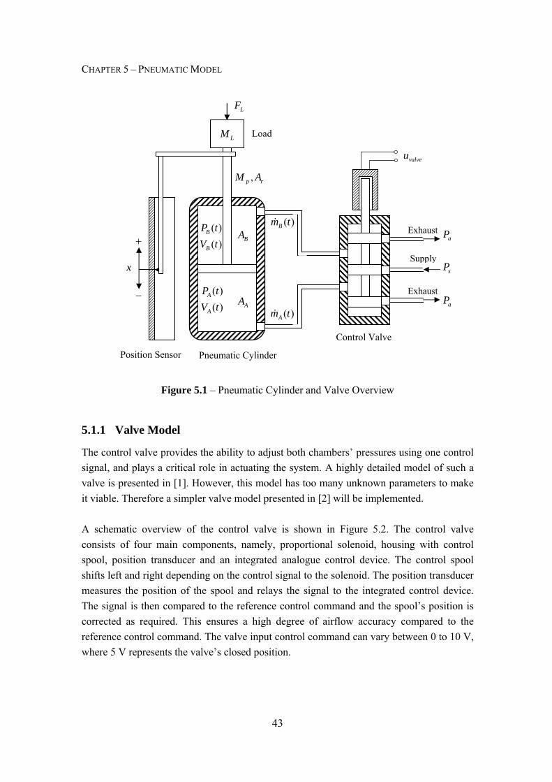
CHAPTER 5 – PNEUMATIC MODEL

43

Figure 5.1 – Pneumatic Cylinder and Valve Overview

5.1.1 Valve Model

The control valve provides the ability to adjust both chambers’ pressures using one control signal, and plays a critical role in actuating the system. A highly detailed model of such a valve is presented in [1]. However, this model has too many unknown parameters to make it viable. Therefore a simpler valve model presented in [2] will be implemented. A schematic overview of the control valve is shown in Figure 5.2. The control valve consists of four main components, namely, proportional solenoid, housing with control spool, position transducer and an integrated analogue control device. The control spool shifts left and right depending on the control signal to the solenoid. The position transducer measures the position of the spool and relays the signal to the integrated control device. The signal is then compared to the reference control command and the spool’s position is corrected as required. This ensures a high degree of airflow accuracy compared to the reference control command. The valve input control command can vary between 0 to 10 V, where 5 V represents the valve’s closed position.

Supply

Exhaust

Exhaust

Pneumatic Cylinder

Control Valve

Position Sensor

Load LM

x

+

−

,p rM A

LF

( )( )

B

B

P tV t

( )( )

A

A

P tV t

BA

AA

( )Bm t

( )Am t

aP

sP

aP

valveu


44

valveumu i

mech.

electr.

Proportionalsolenoid

Controldevice

,A AP m ,B BP mHousing

with spool

aP aPsP

vy

u

Positiontransducer

Figure 5.2 – Proportional Directional Control Valve [2]

Neglecting the solenoid inductance, the proportional relation between the control spool movement vy and valve input valveu is as follows, ( 5)v v valvey C u= − (5.1)

where vC is the valve constant which is defined as /v i nC K R= , where iK is the current gain and nR is the solenoid resistance. The effective area of the valve’s orifice vA is,

2

4v vA y π≈ (5.2)

which is related to the control spool movement and is required to calculate the mass flow rates to and from the pneumatic cylinders, as described in the following section.

5.1.2 Cylinder Chambers Model

The mathematical model for the cylinder chambers was derived using theory presented in [1], [2] and [5]. The equation of the state of ideal gases is, PV mRT= (5.3) assuming that the gas is perfect, where P is a pressure, V is a volume, m is a mass, T is a temperature and R is the ideal gas constant. The mass flow rate, m , of a compressible gas through an orifice can be expressed as,


45

2v um A P

RTψ= (5.4)

where uP is the air pressure at the upstream side of the orifice, T is the air temperature at the inlet, and ψ is the discharge coefficient. The discharge coefficient can be expressed as,

2 1

max

1

0.484

d d

u u

P PP P

κκ κκ

κψ

ψ

+⎧ ⎛ ⎞⎛ ⎞ ⎛ ⎞⎪ ⎜ ⎟−⎜ ⎟ ⎜ ⎟⎪ ⎜ ⎟−⎪ ⎝ ⎠ ⎝ ⎠⎜ ⎟= ⎨ ⎝ ⎠

⎪⎪⎪ =⎩

for

for

dcr

u

dcr

u

P rP

P rP

>

≤

(5.5)

where κ is the specific heat ratio of air, dP is the pressure at the downstream side of the orifice, maxψ is the maximum discharge coefficient of the valve and crr is a critical pressure ratio. Combining equations (5.4) and (5.5), equations can be derived for mass flow rate of air for the cylinder chambers. In the case of subsonic air flow where /d u crP P r> the equation can be expressed as,

2 1

21

d dv u

u u

P Pm A PP P RT

κκ κκ

κ

+⎛ ⎞⎛ ⎞ ⎛ ⎞⎜ ⎟= −⎜ ⎟ ⎜ ⎟⎜ ⎟− ⎝ ⎠ ⎝ ⎠⎜ ⎟⎝ ⎠

(5.6)

The equation for the conservation of mass (continuity) can be written as,

dm d Vdt dt v

⎛ ⎞= ⎜ ⎟⎝ ⎠

2

vV vVmv−

= (5.7)

where v is specific volume. Assuming that the air flow is isentropic, it can be written that,

.Pv constκ = (5.8) Manipulation of equation (5.8) results in the following two equations,

v PvPκ

= − (5.9)


46

1

1c

cPv vP

κ

κ

= (5.10)

where subscript c defines either the atmospheric or supply air pressure states, which are considered as constants. Inserting equations (5.9) and (5.10) into (5.7), the expression for mass flow rate becomes,

11/

1/ 1/c c c c

P PPm V VP v P v

κκ κ

κ κκ

−−

± = ± (5.11)

where mass flow rate can be either positive or negative depending on the direction of the air flow. Selecting the origin of the piston displacement at the middle of the cylinder, the volumes of each of the chambers can be expressed as, 0i i iV V A x= ± (5.12)

i iV A x= ± (5.13)

where i = A, B is the cylinder chambers index, 0iV is the chambers starting volume (including the inactive volume at the end of strokes), iA is the piston effective area and x is the piston position. The difference in cylinder chamber areas is due to the piston rod. Inserting equations (5.12) and (5.13) into (5.11), the expression for mass flow rate becomes,

( )1

1/0

1/ 1/i i i ii i

ic c c c

PP V A xP A xmP v P v

κκ κ

κ κκ

−−

±± = ± (5.14)

The time derivative for the pressures in the cylinder chambers can be obtained from equation (5.14) as,

1/ 1/

0 0

i c c ii i

i i i i

P P v A xP m PV A x V A x

κ κκ κ= ± ±

± ± (5.15)

The first term in the pressure differential equation represents the effects on pressure difference due to the mass flow rate, in or out of the chamber, and the second term represents the pressure difference due to the motion of the piston rod.


47

5.1.3 Piston-Load Dynamics

Considering the equilibrium of forces acting on the piston, the equations of motion can be expressed as,

( )L p f L A A B B a rM M x x F F P A P A P Aβ+ + + + = − − (5.16)

where LM is the external load mass, pM is the piston rod assembly mass, x is the piston position, β is the viscous friction coefficient, fF is the static and Coulomb friction forces,

LF is the external force created due to gravitational acceleration, AP and BP are the pressures in the cylinder chambers, aP is the atmospheric pressure, AA and BA are the piston effective areas and rA is the piston rod cross section area. The friction force has a significant influence on the operation of the pneumatic cylinder, and is dependent on a variety of parameters. Therefore the friction forces were thoroughly researched to obtain an accurate model of their effects on the system. The friction force model was developed from a combination of theory presented in [1] and [4]. It can be noted that the actual friction force differs slightly for extension and retraction of the piston rod. The actual friction also differs slightly depending on the position of the piston rod. These differences are small and for the purpose of this model will be neglected, where the friction force will be considered the same for extension, retraction and at different piston rod positions. The friction force not related to viscous friction, can be expressed as,

( )sgn

sf

f sf

df

FF F

F x

⎧ +⎪= −⎨⎪⎩

ififif

000

xxx

==≠

andand

00

A A B B a r L

A A B B a r

P A P A P A FP A P A P A F

− − − >− − − < (5.17)

where sfF represents the static friction force and dfF represents the Coulomb friction force, and

( )1

sgn 01

x−⎧⎪= ⎨⎪⎩

ififif

000

xxx

<=>

(5.18)

The parameters relating to static and Coulomb friction can be experimentally determined from a simple procedure in [1].


48

5.1.4 Model Validation

The equations developed in Sections 5.1.1 to 5.1.3 can now be combined to complete the nonlinear mathematical model of the system dynamics. The simulation model developed is shown in Figure 5.3.

Figure 5.3 – System Dynamics of the Nonlinear Pneumatic Model It is customary that the accuracy of a model is determined by examining a comparison of the model versus the measured output for a unit input step response. Due to the nonlinearity of the system and due to the system having different characteristics for extension and retraction of the piston rod, a slightly different approach was implemented. A random valve input was commanded in the region of ±1 V from the valve’s normally closed 5 V position. The open loop comparison of the simulated nonlinear pneumatic model and experimental results are shown in Figure 5.4. The model output obtained can be seen to give a reasonable indication of the measured output, although it is found to be slightly inaccurate. There are many parameters that can result in an inaccurate model, such as variations of process parameters during operation. However, it is found that the primary inaccuracies of the model can be attributed to two main reasons: The first reason is that the valve model is inaccurate and does not represent the true dynamics of the valve. To overcome this problem, accurate pressure and flow rate sensors will be required to investigate the actual characteristics of the valve, in order for a detailed valve model to be obtained.


49

0 2 4 6 8 10 12 14 16 18 200.2

0.4

0.6

0.8

1

1.2

x [m

]

Measured outputModel output

0 2 4 6 8 10 12 14 16 18 203.5

4

4.5

5

5.5

6

6.5

u valv

e [V]

Time [s]

Figure 5.4 – Validation of the Nonlinear Pneumatic Model

The second reason is that initial pressures in the cylinder chambers are unknown prior to simulation, and have to be intuitively estimated at a certain steady-state condition. Obtaining accurate pressure sensors will provide the necessary initial cylinder chamber pressures prior to simulation and will also provide a means of validating the accuracy of the pressures obtained in the cylinder chambers model. This was, however, not done in this project due to the costs involved, since high-precision pressure sensors can cost more than the pneumatic actuator itself.

5.2 Simplified Linear Pneumatic Model

The nonlinear model developed in Section 5.1 can be used to gain insight into and understanding of the dynamic pneumatic process. However, for the purpose of classical feedback control, a simpler linear mathematical model is required. The classical approach to obtaining such a linear model is by linearizing the nonlinear system dynamics about a set point, where the model is only valid for small deviations around the operating point. Due to the complexity and inaccuracies of the nonlinear model, a different approach was taken. It can be reasoned that the application of such a model should be considered prior to the development of the model. Essentially, a linear model is required to provide a representation of the behaviour of the plant for classical feedback control synthesis. The control system for this project will primarily be required to track a low frequency (roughly


50

0.2 Hz) sinusoidal reference input signal, discussed in detail in Chapter 8, relating to the motion of a ship at sea. The reference signal changes slowly and it can be considered that mostly small valve openings will be required for regulating the pneumatic cylinder around this reference signal. Therefore this section will focus on obtaining a simplified linear model of the pneumatic process which encapsulates the core dynamics of the system, with focus on obtaining a high degree of accuracy for small valve openings.

5.2.1 Model Derivation and Parameter Identification

The simplified pneumatic system, shown in Figure 5.5, attempts to approximate the pneumatic cylinder as a mechanical mass-spring-damper system. Parameters used in this section are listed in Appendix B.

Figure 5.5 – Simplified Pneumatic System Overview To implement such a mass-spring-damper system, extension and retraction symmetry of the piston rod is required. To obtain this symmetry, two assumptions need to be made:

Position Sensor

Load LM

x

+

−

, 0p rM A =

0LF =

( )( )

B

B

P tV t

( )( )

A

A

P tV t

BA

AA

M

1k

2k

Pneumatic Cylinder Mass-Spring-Damper System

Pressure Plate

2c

1c


51

1. The effects of the piston rod can be neglected and the cylinder can be approximated as a rodless cylinder where rA is equal to zero, which results in BA being equal to AA . This is found to be an acceptable assumption as the piston rod only makes up for approximately 10% of the area of pressure plate and 10% of the volume in chamber A.

2. The external force due to gravitational acceleration can be neglected where LF is equal to zero. This assumption should have a greater effect on the model’s accuracy, where these effects should be noticed with an increase in load mass in a vertical configuration.

It is interesting to note that the two assumptions made partially cancel each other out, where assumption 1 results in an increased downward force and assumption 2 results in a reduced downward force of the model, compared to the actual system. However, the force in assumption 1 is related to pressure BP which is time variant, and the force in assumption 2 is static with a fixed system mass. The approximated mass-spring-damper system is derived from [2] and [3]. The natural frequency of the mass-spring-damper system is expressed as,

nkM

ω = (5.19)

where M is the total system mass in motion ( )L PM M+ , and k is the spring stiffness

1 2( )k k+ expressed as [26],

24 s

T

P AkVκ

= (5.20)

where TV is the total volume of the chambers A and B, sP is the supply pressure and A is the piston effective area ( )A BA A A= = . Inserting (5.20) into (5.19), the natural frequency becomes,

24 s

nT

P AMVκω = (5.21)


52

The damping ratio ς of the cylinder can be expressed as,

22 42T

s

VcP MAMk

βςκ

= = (5.22)

where c is the damping coefficient 1 2( )c c+ , which is equal to viscous friction coefficient β of the pneumatic actuator. The linear differential equation of the cylinder’s motion then becomes, 2 22 n n v n ix x x K uςω ω ω+ + = (5.23)

where u is the control input signal or valve voltage and vK is the velocity gain. The transfer function of the expression in (5.23) can now be expressed as,

( ) ( )( ) ( )

2

2 22v n

pn n

x s KG su s s s s

ωςω ω

= =+ +

(5.24)

The transfer function of the pneumatic cylinder’s dynamics can be considered as a standard second-order mass-spring-damper system, where the added integrator relates to the integral relationship between piston position and control input or valve opening.

The velocity gain, vK , can be determined by an open loop step response, shown in Figure 5.6, where the output is the velocity of the cylinder’s piston and the input is a unit step of the control input signal. Note that the control input u is not the same as the valve input

valveu . The relation between these two input parameters will be discussed in Section 5.2.2.

0 0.5 1 1.5 2 2.5 3 3.5 40

0.05

0.1

0.15

0.2

0.25

0.3

0.35

0.4

0.45

0.5

Time [s]

Vel

ocity

[m/s

]

Measured outputu = 0.5 V Step

0.325 m/s

Figure 5.6 – Open loop Step Response


53

The velocity gain, vK , can be approximated by,

( ) 0.325 / 0.65( ) 0.5v

x t m s mKu t V Vs

= ≈ = (5.25)

Note that the velocity gain term actually varies depending on the control input, due to the nonlinear relation which exists between velocity and the control input. In an endeavour to maintain a simple linear model, this gain is not scheduled and is chosen as a constant. A relatively small control input was commanded as the input step, which effectively linearizes the model about a small valve opening. The open loop poles of the simplified pneumatic model are shown in Figure 5.7. It can be noticed that the core dynamics of the pneumatic system relate to that of the integrator pole, where the effects of the high-frequency dynamics should play a minimal role at low frequencies.

-9 -8 -7 -6 -5 -4 -3 -2 -1 0 1

-20

-10

0

10

20System: GPole : -8.75 + 20.8iDamping: 0.387Overshoot (%): 26.8Frequency (rad/sec): 22.6

System: GPole : 0

Damping: -1Overshoot (%): 0

Frequency (rad/sec): 0

Pole-Zero Map

Real Axis

Imag

inar

y Ax

is

Figure 5.7 – Open loop Poles of the Simplified Pneumatic Model

5.2.2 Friction Function

The friction force has a significant influence on the operation of the pneumatic cylinder and the unmodelled static and Coulomb friction forces will have to be considered prior to model validation of the simplified model.

The proposed solution is to create a friction function which essentially offsets the valve’s input voltage, valveu , at a plant level in order that the valve will always open in either direction, with an offset to compensate for the effects of static friction. This essentially removes the effects of static and Coulomb friction on the piston rod, in an open loop fashion. The friction function also provides a means to compensate for unmodelled valve


54

dynamics as well as variations in static friction for extension and retraction of the piston rod. A block diagram which depicts the implementation of the friction function is shown in Figure 5.8.

Figure 5.8 – Friction Function Block Diagram To determine the required offsets of the valve the effects of the static friction will first have to be investigated. This is done by slowly opening the valve at a linear rate, in either direction, from the valve’s normally closed position, where the initial piston rod starting position is located in the middle of the available stroke length. The position and velocity results obtained are shown in Figure 5.9. Note the nonlinear relation between valve opening and velocity.

4 6 8 10 12 140.6

0.65

0.7

x [m

]

4 6 8 10 12 145.2

5.4

5.6

u valv

e [V]

Time [s]

X: 11.61Y: 5.58

4 6 8 10 12 140

0.05

0.1

x_do

t [m

/s]

6 8 10 12 14 16 180.5

0.55

0.6

0.65

6 8 10 12 14 16 18

4.2

4.4

4.6

4.8

Time [s]

X: 15.99Y: 4.2

6 8 10 12 14 16 18

-0.1

-0.05

0

0.05

Figure 5.9 – Static Friction Effect

It can clearly be seen how the piston rod has to numerously overcome the effects of static friction due to the dynamics of the system. This is due to the pressure difference in the two

Friction Function Plant

valveu

modelx u

measuredx

Model


55

chambers, which slowly increases until a force high enough to overcome the static friction is obtained. Once this occurs the piston rod moves, which results in a reduced pressure difference and the piston rod becomes stationary again. It is proposed that the initial valve offsets is chosen at a voltage where the mean velocity is approximately 2.5 cm/s, to ensure that the effects of static friction will be avoided under most operating conditions. It can be noted that the valve voltage offsets essentially limits the system’s minimum obtainable velocity in either direction.

The friction function relation between control input u and the valve input valveu is shown in Figure 5.10. At a control input of zero, the valve remains closed and as the control input increases or decreases, the valve will start opening linearly from its offset value. When the valve reaches the maximum open position, it will saturate and remain at this value for the upper and lower limits of the control input values. This saturation region relates to the amount of offset that is present on the valve.

-5 -4 -3 -2 -1 0 1 2 3 4 50

1

2

3

4

5

6

7

8

9

10

u valv

e [V]

u [V]

uvalve = 5.58 V

uvalve = 4.2 V

Figure 5.10 – Friction Function Control Input Relation The friction function could create possible control problems when a constant reference position is required, where the control input will operate around a zero volt range. This will create possible vibration and wear on the valve, as the valve jumps between the upper and lower offset values. This problem will be addressed in Chapter 6. The implementation of the friction function plays a critical role in the ability to accurately track a sinusoidal reference input signal, which is the primary reference input for simulating the motion of a ship at sea. The influence and benefits of the friction function will be discussed in Chapter 6 as well.


56

5.2.3 Model Validation

The simplified linear pneumatic model developed in Section 5.2.1, with implementation of the friction function before the plant, can now be used to validate the performance of the model. Similarly to that of the nonlinear model, a random valve input will be commanded in the region of ±1 V from the valve’s normally closed 5 V position. This provides a better comparison than a unit input step response, due to the nonlinearity of the system and due to the system having different characteristics for extension and retraction of the piston rod. The friction function valve offsets and the model’s viscous friction coefficient were carefully fine-tuned to obtain the best possible comparison between the model and the plant. It was found that the results obtained were extremely sensitive to small changes made to the valve offsets. The open loop comparison of the simulated simplified linear pneumatic model and experimental results are shown in Figure 5.11. Note that the input signal is the control input and not the valve input.

0 2 4 6 8 10 12 14 16 18 200.2

0.4

0.6

0.8

1

1.2

x [m

]

Measured outputModel output

0 2 4 6 8 10 12 14 16 18 20-0.5

0

0.5

u [V

]

Time [s]

Figure 5.11 – Validation of the Simplified Linear Pneumatic Model

The modelled output obtained can be seen to give an excellent representation of the measured output, which is more accurate than that of the nonlinear model. The drawback of this model is that it only represents the measured output accurately for small valve openings, where the total system mass and supply pressure remain constant under operation. The effects of operating at larger valve openings are shown in Figure 5.12.


57

0 0.5 1 1.5 2 2.5 30

0.2

0.4

0.6

0.8

x [m

]

0 0.5 1 1.5 2 2.5 30

0.2

0.4

0.6

0.8

1

u [V

]

Time [s]

0 0.5 1 1.5 2 2.5 30.2

0.4

0.6

0.8

1

1.2

0 0.5 1 1.5 2 2.5 3-1

-0.8

-0.6

-0.4

-0.2

0

Time [s]

Measured output Model output

Figure 5.12 – Nonlinear inaccuracies of the Simplified Linear Pneumatic Model

The inaccuracies of the simplified linear model at larger valve openings can be attributed to many reasons such as the unmodelled nonlinear dynamics associated with air compressibility as well as the two symmetry assumptions made in Section 5.2.1, which result in varying steady state conditions for extension and retraction of the piston rod. It is considered that the primary and more dominant reason for inaccuracies at large valve openings is due to the velocity gain, vK , being chosen as a constant value, where this gain is actually a variable parameter relating primarily to valve opening. This results in increasing inaccuracies at larger valve openings. The velocity gain, vK , could be updated with parameters such as control input and taken into account in the controller design, although model differences did not warrant the extra complexity.

5.3 Summary

In this chapter, two mathematical models of the linear pneumatic actuator were presented. A complex nonlinear model of the pneumatic actuator was developed, which was found to give a reasonable indication of the plant’s output, although slightly inaccurate. A simplified control-orientated linear model of the pneumatic actuator was also developed, which was found to give an excellent indication of the plant’s output. This model is, however, only accurate for small control inputs or valve openings. The design of a pneumatic positioning control system will be considered in Chapter 6.

58

Chapter 6

Pneumatic Control In this chapter, the control system required to enable the pneumatic cylinder to track a desired position reference, will be considered. A description of the experimental setup used to test the controller will be presented in Section 6.1. Initial attempts at the implementation of various linear control architectures, were found to deliver poor results, primarily due to the significant system nonlinearities present in the pneumatic system. Considering this, a sliding mode controller design was used which will be discussed in Section 6.2. Furthermore, two logic control functions developed to increase overall controller performance will be described in Section 6.3 and Section 6.4. The controller’s overall performance, applied to multiple scenarios, will be evaluated in Section 6.5.

6.1 Description of Experimental Setup

A photo of the experimental setup of a single linear pneumatic actuator is shown in Figure 6.1. The experimental setup can be seen to consist of components discussed in Chapter 3 and Chapter 4. A test rig, consisting of the linear pneumatic actuator in a vertical setup, proportional directional control valve as well as the pneumatic control electronics module, was created. The test rig can be seen on the left of the photo. On the right of the photo, the battery pack used to power the system, as well as a computer required to interface to the test rig, can be seen. A departmental 7 bar air pressure point was used to power the pneumatic cylinder.

CHAPTER 6 – PNEUMATIC CONTROL

59

Figure 6.1 – Experimental Setup The test rig was created to evaluate the performance and accuracies that can be achieved by the pneumatic actuator prior to the purchase and build-up of the complete motion simulation platform, as discussed in Chapter 3. This also creates the ability to test the majority of the system including mechanical hardware, electrical hardware and software. The creation of this fully operational single actuator will minimise risk and assist in the final build-up of the motion simulation platform, as opposed to building the motion simulation platform without prior testing.

6.2 Sliding Mode Control Design

Sliding mode control (SLMC) has been promoted as a robust control technique which is able to overcome significant system nonlinearities associated with pneumatic positioning systems [6]. According to [8], a SLM controller can make a nonlinear system behave as a linear system once the states of the system reach and track the so-called sliding surface. SLMC reportedly has several benefits such as a fast response, low sensitivity to disturbances and

Computer

Battery Pack

Proportional Directional

Control Valve Pneumatic

Control Electronics

Module

Linear Pneumatic Actuator


60

system parameter variations. According to [9], SLMC theory was adopted for a pneumatic force actuator system because of its robustness and good performance even for highly nonlinear systems. According to [6], SLMC practically does not need an explicit model of the system and has a low sensitivity to disturbances. As a result of these advantages, it could be implemented successfully in less demanding industrial applications. Considering the above mentioned results, a sliding mode controller developed in [8] and [6] for a pneumatic actuator was adopted as the initial control system to be implemented on the linear pneumatic actuator. In [8] it was found that SLMC was able to maintain performance when the load mass was varied upwards by a factor of 10. This is highly desirable for an application such as a motion simulation platform. The control law for SLMC can be given as, sgn( )eu V σ= − −K x (6.1)

with eK as gain, x as state vectors, V as the maximum supply voltage to the control valve (5V in this case) and σ as the switching function. According to [8], in applications where stability in not an issue, omission of the first term often has a minimal effect on the system response, and is often ignored by authors.

For a third-order pneumatic positioning system, the switching function σ can be given as, 1 2( )Rc x x c x xσ = = − − + +Gx (6.2)

where x is the piston position and G is the vector that defines the sliding surface as dictated by coefficients 1c and 2c . It can be noted that both the velocity and acceleration must be available for this implementation.

The SLMC design in equations (6.1) and (6.2) could prove to be inadequate due to undesired excessive chattering in the control signal u once the sliding surface is reached, when 0σ ≈ . This may excite unmodelled high-frequency dynamics. Chattering is generally undesired due to negative effects on switching control components and may cause premature wearing and damage to system components. However, in many applications chattering is not a problem as in PWM systems, where chattering is inherent to the control action. In some applications, chattering acts as a dither signal to overcome or reduce effects such as static friction.


61

A common technique used to eliminate chattering is achieved by smoothing out the control discontinuity, where the basic control law in equation (6.1) is modified to include a boundary layer [7] neighbouring the switching surface so that, sat( )u V σ= − (6.3)

where the saturation function is defined as,

( )sgn /sat( )

/σ φ

σσ φ

⎧= ⎨⎩

ifif

σ φσ φ

>≤

(6.4)

where φ is the boundary layer ‘thickness’. The saturation function and boundary layer are graphically illustrated in Figure 6.2.

Figure 6.2 – Saturation Function and Boundary layer Note that the eK x term has been ignored. The boundary layer of φ can be used to find the proper balance between minimal chattering and acceptable accuracy. It can be noted that when the system enters the boundary layer, the SLMC action becomes equivalent to that of a state feedback controller of the form,

[ ]1 2 1Rx x

Vu c c xx

φ

−⎡ ⎤⎛ ⎞ ⎢ ⎥= − = − − ×⎜ ⎟ ⎢ ⎥⎝ ⎠ ⎢ ⎥⎣ ⎦

Kx (6.5)

where K and x are the gain and state vector, respectively.

σ

/u V−

σ φ=

1

1−

σ φ= −

Boundary layer


62

A block diagram of the final pneumatic position controller using SLMC is shown in Figure 6.3. The initial values for coefficients 1c and 2c are chosen as 2

1 nc ω= and 2 2 nc ςω= as in [6]. The sampling frequency of the controller was chosen at 100 Hz, which is approximately 28 times faster than that of the fastest dynamics of the simplified linear pneumatic model, presented in Chapter 5. The effects of the friction function and reference monitoring blocks have not yet been considered and will be discussed in detail in Section 6.3 and Section 6.4 respectively. The two low-pass filters located on the feedback measurement signals will be discussed next in Section 6.2.1. It can be noted that the final controller as described in Figure 6.3 was programmed onto the microcontroller of the pneumatic control electronics module, where the low-pass filters and differentiation blocks were discretized and the rest of the controller was implemented using emulation, due to the high sampling frequency.

Figure 6.3 – Block Diagram of the Pneumatic Position Control

6.2.1 Feedback Measurement Filtering

In practical realization of pneumatic systems it is generally acknowledged that both velocity and acceleration feedback are essential to ensure adequate positioning performance [8]. At this point in the design, the only measurement available for feedback is

x

V−

s

1c

( )2

2 22v n

n n

Ks s s

ωςω ω+ +

2 nςω

( )sat σ

x

Rx

s

2nω−

1

1sωω+

2

2sωω+

Plant Friction Function

Reference Monitoring

x

2c

u

valveu

σ Experimental

or Simulation

Indicates changes made to existing Sliding Mode Control Design

_ +


63

that of the displacement sensor discussed in Chapter 3. Acceleration, which can easily be integrated to velocity, can be obtained from three possible methods:

1. The first method is to directly measure acceleration of the piston rod with a precision accelerometer. This can, however, be costly and complications could arise from the coupling of gravitational acceleration when the pneumatic cylinder is not constrained in a vertical or horizontal configuration, where the exact orientation of the pneumatic cylinder might be unknown.

2. The second method is to measure the pressure difference between cylinder chambers, where the acceleration can be obtained from the equilibrium of forces acting on the piston, as in (5.16). However, this will require the external forces as well as the friction forces acting on the piston to be known. Alternatively, these forces can be neglected, which will result in the diminished accuracy of the acceleration measurement. The accurate measurement of pressure can also be costly depending on the pressure sensor.

3. The third method is to double differentiate the piston position measurement to obtain acceleration. This, however, generally produces an acceleration signal with large noise levels.

Method three was selected as an initial means to obtain acceleration, due to the fact that no costs are involved and a position measurement with high resolution and accuracy is available. Method one or two can always be added in future research, if desired. As stated in method three, large noise levels were found when differentiating from position to velocity and from velocity to acceleration. The displacement sensor developed was found to produce an excellent position measurement, free from any drift. The measurement signal, however, still contains a small amount of quantization noise due to the signal originating from a digital optical encoder, which can only output at finite position increments. The differentiation noise is created due to this quantization noise where there is a constant gradient change of the position measurement between time steps. It was therefore required to low-pass filter the position measurement to create a smooth gradient change, thereby dramatically lessening the effects of the signal noise, due to differentiation. The velocity signal was also low-pass filtered to reduce any further unwanted noise when differentiating to acceleration. It can be noted that the higher the position measurement resolution, the less the noise created by differentiation will be.


64

The cut-off frequency of the first-order low-pass filters were chosen as 1 50ω = rad/s and

2 100ω = rad/s from practical findings, where changing the cut-off frequency of these filters essentially creates a trade-off between feedback measurement phase lag and differentiated signal noise levels. To investigate how these filters affect the developed controller, the closed loop poles of the system can be investigated with and without the feedback measurement filtering, as shown in Figure 6.4. It is important to note that these poles only give an indication of the true system dynamics and are only valid for small valve openings or control inputs. It can be seen that the filters do not have a considerable effect on the system’s closed loop poles. The most noticeable effect is that of the system’s most dominant pole shifting from 6.7 rad/s to 8 rad/s when the filters are added. It should be noted that the filters will definitely have a negative effect on the controller’s performance. However, they play an essential role in reducing feedback acceleration and velocity noise levels.

-9 -8 -7 -6 -5 -4 -3 -2 -1 0-25

-20

-15

-10

-5

0

5

10

15

20

25

System: G_clPole : -8.75 + 20.8iDamping: 0.387Overshoot (%): 26.8Frequency (rad/sec): 22.6

System: G_clPole : -6.65Damping: 1Overshoot (%): 0Frequency (rad/sec): 6.65

Closed Loop Poles - Without Feedback Measurement Filtering

Real Axis

Imag

inar

y Ax

is

-120 -100 -80 -60 -40 -20 0

-25

-20

-15

-10

-5

0

5

10

15

20

25

System: G_cl_fPole : -8.01Damping: 1

Overshoot (%): 0Frequency (rad/sec): 8.01

System: G_cl_fPole : -9.11 + 22.1i

Damping: 0.381Overshoot (%): 27.4

Frequency (rad/sec): 23.9

Closed Loop Poles - With Feedback Measurement Filtering

Real Axis

Imag

inar

y Ax

is

Figure 6.4 – Closed Loop Poles at ϕ=250

6.2.2 Simulation and Practical Results

Simulated step responses of the piston position control, as well as the control input are shown in Figure 6.5. Note that the effects of the friction function and reference monitoring blocks have not yet been considered in the results presented in this section.


65

0 1 2 3 4 5 6 70.2

0.4

0.6

0.8

1

x [m

]

xR

(t) x(t) φ=100 x(t) φ=250 x(t) φ=400

0 1 2 3 4 5 6 7-5

0

5

u [V

]

Time [s]

φ=100φ=250φ=400

Figure 6.5 – Simulation results of Piston Position Control

The effects of varying φ can be seen, where a reduction in φ results in a reduced boundary layer, which essentially increases the total feedback gain. It can be observed that the SLMC operates primarily within the boundary layer, where attempts to reduce the boundary layer result in increased oscillations on position. This could be as a result of the dynamics of the controller where unwanted phase lag is introduced to the feedback measurements. The controller’s performance can now be carefully tested and evaluated in simulation. However, due to the vast differences found between the simulation and practical results, which are primarily due to the significant system nonlinearities, a more practical approach is used to evaluate and test the controller’s performance, where tests are mostly performed on the actual plant with minimal simulation. It should be noted that the simplified linear pneumatic model is only valid for small valve openings, when used in conjunction with the friction function, as developed in Chapter 5. The controller’s performance will be evaluated and configured primarily on a sinusoidal reference input with a frequency of 1.2 rad/s, which relates to the motion of a ship at sea, as discussed in Chapter 8. It can be noted that the controller can be configured to perform well for reference step responses, although when this same controller configuration is used to track a sinusoidal reference signal, results may differ to a great extent.

The practical sinusoidal reference tracking ability of the controller at 1.2 rad/s with variation in φ , is shown in Figure 6.6.


66

0 1 2 3 4 5 6 7 80.2

0.4

0.6

0.8

1

x [m

]xR(t)

x(t) φ=90x(t) φ=150x(t) φ=350

0 1 2 3 4 5 6 7 8-2

-1

0

1

2

u valv

e [V]

Time [s]

φ=90φ=150φ=350

Figure 6.6 – Practical Sinusoidal Reference Tracking at 1.2 rad/s

It can be seen that the controller struggles to track the maximum and minimum points of the sinusoidal reference signal, where the piston is required to stop and change direction. This can be attributed to the existence of static and Coulomb friction on the piston rod. It can be noted that, as in simulation, reducing the boundary layer only creates an oscillation on position and does not solve the effects of friction. A solution to the undesired effects of friction will be discussed in Section 6.3.

6.3 Friction Function

The friction function, developed in Chapter 5, was required to essentially remove the effects of static and Coulomb friction on the piston rod, by creating an offset on valve input voltage or control command. This effectively limits the minimum allowable velocity of the piston in either direction. It can be noted that slight changes to these valve offset values have a considerable effect on the controller’s sinusoidal tracking ability. The implementation of the friction function can be seen to effectively change the saturation function of equation (6.4), as shown in Figure 6.7. The left graph relates to the saturation function in simulation, while the right graph illustrates the effective change to the saturation function due to the friction function. The offsets around the σ axis relate to the voltage offsets chosen in the friction function, by factor five which is equal to that of the maximum supply voltage of the control valve.


67

Figure 6.7 – Effective Saturation Function change with Friction Function

The friction function was found to play a vital role in the controller’s ability to accurately track a sinusoidal reference input by effectively reducing some of the system nonlinearities present in the plant. The practical sinusoidal tracking results of the controller, with and without the implementation of the friction function, are shown in Figure 6.8. The position measurement with 250φ = corresponds with when the friction function was implemented. It can be observed that the tracking ability of the controller is significantly improved with the aid of the friction function and will therefore be integrated into the control architecture.

0 1 2 3 4 5 6 7 80.2

0.4

0.6

0.8

1

x [m

]

xR(t)

x(t) φ=150x(t) φ=250

0 1 2 3 4 5 6 7 8-2

-1

0

1

2

u valv

e [V]

Time [s]

φ=150

φ=250

Figure 6.8 – Friction Function effects on Sinusoidal Tracking at 1.2 rad/s

σ

/u V−

σ φ=

1

1−

σ

/u V−

σ φ=

1

1−


68

A reasonable amount of phase lag, in the order of 140 ms, can be observed between the reference signal and the output measurement. However, phase lag can be considered not to be problematic when simulating the motion of a ship, as it simply results in the desired motion of the ship being simulated to be slightly delayed, although correct. It should be noted that a smooth output signal, which more accurately represents that of the reference, is favoured above the occurrence of phase lag. Phase distortion, however, is undesirable as this will warp the measured output in comparison with the reference, although when simulating the frequencies relating to the motion of a ship at sea, as discussed in Chapter 8, this error is found to be insignificant.

In Figure 6.9, the sinusoidal reference tracking ability of the controller with 250φ = is shown, where the reference signal has been shifted over the measured position signal by adding a constant delay to the reference signal, in order to obtain an indication of the position error between the reference and output signal. This has been done to create a means to quantify how well the reference is actually being tracked. The controller’s performance can be considered to be more than adequate with a measured position error within a 5 mm bound, with an RMS value of about 1.6 mm. It can be noted that the error is only an indication of the controller’s performance, where a slight change in reference delay will change the error signal considerably.

0 1 2 3 4 5 6 7 80.2

0.4

0.6

0.8

1

x [m

]

xR(t)

x(t)

0 1 2 3 4 5 6 7 8-6

-4

-2

0

2

4

x err [m

m]

Time [s]

xerr(RMS)=1.606mm

Figure 6.9 – Sinusoidal Tracking at 1.2 rad/s with Reference Delay


69

6.4 Reference Monitoring

Reference monitoring was introduced to minimise high frequency vibration and wear on the control valve caused by chattering in the control signal, valveu . This occurs when the controller is tracking a constant reference which results in a constantly changing control signal and piston position. This unwanted chatter originates from the valve voltage offsets as developed in the friction function, where the valve is constantly commanded between its upper and lower offset values. The ability to accurately track a constant reference position is not of vital importance when simulating the motion of a ship, as the reference will almost always be constantly changing. However, the controller must still have the ability to track a constant reference. The reference monitoring essentially monitors the reference position signal and when the signal is determined to be the same for more than 10 time steps, it enables a function that sets the valve to its zero point when the error between the reference and actual position output is less than 2 mm. As soon as the reference changes, this function will again be disabled. The effects of reference monitoring are shown in Figure 6.10.

0 1 2 3 4 5 6 70

0.2

0.4

0.6

0.8

1

x [m

]

Time [s]

xR(t) x(t) x(t) With References Monitoring

0 2 4 6-5

0

5

u valv

e [V]

Time [s]0 2 4 6

-4

-2

0

2

4

x err [m

m]

Time [s]

Figure 6.10 – Reference Monitoring Results It can be argued that this constant control activity could in some cases be necessary to achieve a high level of controller performance. However, in this case this is not required nor does it deliver any additional positioning accuracy.


70

6.5 Evaluation of Practical Results

In this section the controller’s performance will be evaluated in three scenarios. The first scenario will evaluate the controller’s ability to track a position reference at various frequencies with increasing amplitude. The second scenario will evaluate the effect of additional mass on the system, while the third scenario will evaluate the controller’s tracking ability on a snippet of ship heave data created in Chapter 8. It can be noted that in all these results 250φ = and the reference signal has been shifted over the measured position signal to obtain an indication of the error that occurs. The controller was tested with a sinusoidal reference of up to 6 rad/s, although at this frequency, it was found that the tracking ability of the controller diminishes dramatically where a reduced output amplitude was recorded. In general, it was found that larger position errors occur with a position reference of higher amplitude and frequency, where larger control inputs or valve openings are commanded. This is to be expected when the dynamics of the system are considered, where a larger and faster position change will require the creation of a larger error. It should also be noted that the model created is only accurate for small valve openings and becomes increasingly inaccurate with larger valve opening. To reduce these errors at larger valve openings, without inducing oscillation into the system, it could be proposed to increase the valve opening or control input nonlinearly according to the amount of total feedback or position error measured, where changes could be made to the friction function or saturation function. However, the controller is generally found to perform adequately and will only be tested further once all the pneumatic cylinders have been integrated into the motion simulation platform, where all the cylinders will have to share the same pressure supply.

6.5.1 Sinusoidal Tracking

The controller’s tracking ability of a sinusoidal reference with increasing amplitude at 0.5, 1.2 and 2 rad/s, is shown in Figure 6.11, Figure 6.12 and Figure 6.13 respectively.

The effects of chattering in the control signal valveu can also be noticed at low position amplitudes, due to the valve offsets imposed by the friction function, where position is found to change minimally over time. This is generally undesired, although necessary to obtain acceptable position accuracies.


71

0 5 10 15 20 25 30 35 40 450

0.5

1

x [m

]

xR

(t) x(t)

0 5 10 15 20 25 30 35 40 45

-1

0

1

u valv

e [V]

0 5 10 15 20 25 30 35 40 45-5

0

5

x err [m

m]

Time [s]

xerr

(RMS)=1.37mm

Figure 6.11 – Sinusoidal Tracking with Increasing Amplitude at 0.5 rad/s

0 5 10 15 20 25 30 35 400

0.5

1

x [m

]

xR

(t) x(t)

0 5 10 15 20 25 30 35 40-2

0

2

u valv

e [V]

0 5 10 15 20 25 30 35 40-10

0

10

x err [m

m]

Time [s]

xerr

(RMS)=1.91mm

Figure 6.12 – Sinusoidal Tracking with Increasing Amplitude at 1.2 rad/s


72

0 5 10 15 20 25 300

0.5

1

x [m

]

xR

(t) x(t)

0 5 10 15 20 25 30

-2

0

2

u valv

e [V]

0 5 10 15 20 25 30-20

0

20

x err [m

m]

Time [s]

xerr

(RMS)=3.87mm

Figure 6.13 – Sinusoidal Tracking with Increasing Amplitude at 2 rad/s

6.5.2 Sinusoidal Tracking with Mass

The controller’s tracking ability of a sinusoidal reference, with and without an added 10 kg mass, at 1.2 rad/s, is shown in Figure 6.14. It can be seen that almost no change is found when the mass is added to the system, where the 10 kg mass relates to a 50% total mass increase. The fact that the two outputs were found to be so similar, proves that the motion simulation platform should be able to operate successfully with a variation in mass.

0 1 2 3 4 5 6 7 80.2

0.4

0.6

0.8

1

x [m

]

xR

(t) x(t) x(t) With added 10kg mass

0 1 2 3 4 5 6 7 8

-4

-2

0

2

4

6

8

u valv

e [V]

Time [s]

xerr

(RMS)=1.98mm xerr

(RMS)=1.91mm

Figure 6.14 – Sinusoidal Tracking with an Increase in Mass at 1.2 rad/s


73

6.5.3 Ship Heave Motion Tracking

The controller’s tracking ability of a snippet of ship heave data is shown in Figure 6.15.

0 5 10 15 20 25 30 35 40 450

0.2

0.4

0.6

0.8

1

x [m

]

0 5 10 15 20 25 30 35 40 45

-10

-5

0

5

10

x err [m

m]

Time [s]

xR

(t) x(t)

xerr

(RMS)=3.71mm

Figure 6.15 – Ship Heave Motion Tracking

Heave data is used to test the controller as this will be the primary reference signal that the controller will be required to track on all three of the pneumatic cylinders of the motion simulation platform, where roll and pitch only create small variations in this signal. The exact origin of this heave data will be discussed in detail in Chapter 8.

6.6 Summary

In this chapter, the design of a pneumatic position control system was presented and discussed. A sliding mode controller modified with a boundary layer, with added friction compensation and feedback filtering, was implemented on the pneumatic cylinder. The final controller which only obtained feedback from a position measurement was evaluated via practical results, where these results were found to be acceptable for use in the initial implementation of the motion simulation platform. Further improvements and expansion of the controller, through more accurate feedback measurements or by increasing the valve opening or control input nonlinearly, according to the amount of total feedback or position error measured, will result in increased position accuracy.

74

Chapter 7

Platform Model and Control In this chapter, the modelling and control of the developed motion simulation platform will be considered. In Section 7.1, a platform orientation model, developed to convert a desired ship orientation to the piston stroke of the three linear pneumatic actuators, and vice versa, will be discussed. In Section 7.2, the full control of the motion simulation platform will be discussed and results will be evaluated. The pneumatic position controller design, discussed in Chapter 6, will be used to control each of the three linear pneumatic actuators.

7.1 Platform Orientation Model

The platform orientation model is required to create the ability to convert a certain ship orientation to the piston stroke of the three pneumatic cylinders of which the motion simulation platform is comprised. This model is also required to convert the three piston strokes back to a ship orientation. These conversions are required to enable the full control of the motion simulation platform. The desired orientation or degrees of freedom of the ship to be simulated by the motion simulation platform are shown in Figure 7.1. A detailed description of the ship’s full axis system, which relates to the ship motion data obtained, is presented in Appendix C.

Figure 7.1 – Ship Orientation

Heave Pitch Roll

Φ Θ

H

CHAPTER 7 – PLATFORM MODEL AND CONTROL

75

The ship’s attitude is represented by the most commonly used Euler 3-2-1 angle sequence of yaw, pitch and then roll, where yaw is ignored for this application. This implies that the third rotation angle is defined as a roll and is about a vector created by the yaw and pitch angles. A detailed description of Euler angles and rotation sequences can be found in [10], [11] and [12]. A block diagram of the platform orientation model is shown in Figure 7.2, which describes the inputs and outputs of two mathematical function blocks created.

Figure 7.2 – Platform Orientation Model Block Diagram

In the block diagram 1p , 2p and 3p relate to the piston stroke of the relevant pneumatic cylinder and H , Θ and Φ relate to the ship’s heave, pitch and roll respectively.

7.1.1 Platform Parameter Definition and Constraint Equations

The platform parameters will now be defined and constraint equations will be derived to create a mathematical means of describing the motion simulation platform’s operation. An overview of the platform’s orientation is shown in Figure 7.3, where H , φ and θ represent the platform’s heave, pitch and roll respectively. Note that the platform’s pitch and roll angles are defined in the opposite direction to that of the ship’s orientation.

To define the platform parameters, the platform is considered in two 2D planes, namely, the front view plane and side view plane, as indicated in

Figure 7.3. A detailed description of these two planes, which indicate the variables required to define the platform’s operation, is shown in Figure 7.4.

The front view plane is chosen as a 2D plane in which pneumatic cylinders one and two are constrained, and the side view plane is chosen as a 2D plane in which pneumatic cylinder three is constrained. In each plane the x and y axes are defined as, x in the horizontal direction and y in the vertical direction.

Ship Orientation

to Piston Stroke

Piston Stroke

to Ship

Orientation

H

Φ

Θ

H

Φ

Θ

1p

2p

3p

1p

2p

3p


76

1P 2P

1 1( , )x y 2 2( , )x y ( , )b h

12L

2( ,0)L

(0,0)

22L 2( ,0)L−

3P h

(0, )h 3 3( , )x y

3L

4( ,0)L 4L

(0,0)

1P 2P

1 1( , )x y

2 2( , )x y ( , )b h

θ

(0,0)

2( ,0)L

3P h

(0, )h

3 3( , )x y

(0,0)

4( ,0)L

a

2( ,0)L−

Figure 7.3 – Platform Orientation

Figure 7.4 – Motion Simulation Platform Constraint Planes

90° Front View

Side View

Front View Plane Side View Plane

90° 90°

Heave Pitch

Roll

Ship Forward Direction

φ

θ

H

1P

2P

3P


77

θ3 3( , )x y

The pitch of the platform can, however, not be defined in the front view or side view planes, due to the design of the platform, and is defined as an angle relative to the platform’s roll angle as shown in Figure 7.5. Defining the pitch in this way results in the platform’s attitude being represented by an Euler 3-1-2 angle sequence of yaw, roll and then pitch, where yaw is again ignored for this application. This implies that the third rotation angle is defined as a pitch and is about a vector created by the yaw and roll angles.

Figure 7.5 – Definition of the Platform Pitch Angle The centre point of the platform is defined as a point in the front view plane which is located exactly between the upper ends of pneumatic cylinders one and two. It can be noted that a small amount of undesired sway, defined as b, exists at this chosen centre point. This sway term only becomes a non-zero term when a non-zero platform roll and pitch occur simultaneously. The undesired sway term which occurs at the chosen centre point is due to the constraints imposed on the pneumatic cylinders by the mechanical design of the motion simulation platform. The mechanical design of the motion simulation platform does not accommodate for a possible centre point, on the top platform, which is constrained in a horizontal plane. It can be noted that as the chosen centre point is moved from its current position towards the upper end of pneumatic cylinder three, the effects of sway become less and the effects of surge become more. When the centre point is located on the upper end of pneumatic cylinder three, the effects of sway become zero and only the effects of surge are present. To create a perfect centre point free from any sway and surge, the design of the motion simulation platform would have to be altered to enforce a certain fixed centre point. However, as discussed in Chapter 2, this was not done to retain a relatively simple mechanical design and to reduce design costs, where the effects of coupling into undesired

φ

3L

a

b

Front View

Side View

Front View Plane

Side View Plane


78

degrees of freedom were assumed to be small and expected to have a minimal effect on the application of the motion simulation platform. The effects of the undesired coupling will be further discussed in Section 7.1.4.

The variables defined in Figure 7.4 and Figure 7.5 can be used to derive multiple constraint equations which define the motion simulation platform’s operation. The variables ix and

iy , where 1,2,3i = is the pneumatic cylinder number, are derived as, 1 1 cosx b L θ= − (7.1)

1 1 siny h L θ= − (7.2)

2 1 cosx b L θ= + (7.3) 2 1 siny h L θ= + (7.4)

3 3 cosx L φ= (7.5)

3y a h= + (7.6)

where the variables a and b are derived as, 3 sin cosa L φ θ= (7.7)

3 sin sinb L φ θ= (7.8)

The variable iP is the total length of the relevant linear pneumatic actuator, defined as, 0i iP p p= + (7.9)

where ip is the piston stroke and 0p is the offset length of the linear pneumatic actuator at a zero piston stroke. The height h of the platform’s centre point is defined as, 0h h H= + (7.10)


79

where H is the simulated heave of the platform and 0h is the offset height from the ground zero reference point to the platform’s centre point. Note that 0h h= when all three of the pneumatic cylinders are at zero stroke length. A table of constant parameters relating to the design of the motion simulation platform discussed in Chapter 3 are presented in Appendix B.

7.1.2 Ship Orientation to Piston Stroke

In this section, a mathematical means will be derived to calculate the three piston strokes from a certain known ship orientation. Firstly, it is required to convert the attitude of the ship, which is defined in an Euler 3-2-1 angle sequence, to the attitude of the platform, which is defined in an Euler 3-1-2 angle sequence. To enable this conversion, it is necessary to describe the attitude of the ship’s axis system by means of a 3×3 rotation matrix. The rotation matrix for an Euler 3-2-1 angle sequence, which relates to the attitude of the ship, can be written [10] as,

321

321

cos 0 sin( 0, , ) sin sin cos cos sin

sin cos sin cos cosR

Θ Θ⎡ ⎤⎢ ⎥Ψ = −Θ −Φ = Θ Φ Φ − Θ Φ⎢ ⎥⎢ ⎥− Θ Φ Φ Θ Φ⎣ ⎦

(7.11)

where a −Θ and −Φ are inserted into the Euler 3-2-1 rotation matrix to rotate the ship's axis system with the x-axis facing forward. This is done in order for the resulting axis system to coincide with the definition of that of the platform’s axis system. The attitude of the platform in an Euler 3-1-2 angle sequence can now be obtained from the ship’s Euler 3-2-1 rotation matrix and can be written [10] as,

( )( )

( )

13 33

23

21 22312

arctan 2 ,arcsin

arctan 2 ,

r rrr r

φθψ

⎡ ⎤−⎡ ⎤⎢ ⎥⎢ ⎥ = ⎢ ⎥⎢ ⎥⎢ ⎥⎢ ⎥ −⎣ ⎦ ⎣ ⎦

(7.12)

where xyr represents components of the ship’s Euler 3-2-1 rotation matrix, where x indicates the row and y indicates the column of the rotation matrix. Note that when converting from the ship’s Euler 3-2-1 angle sequence to the platform’s Euler 3-1-2 angle sequence, a non-zero yaw term, ψ , can be created in the platform’s Euler 3-1-2 angle sequence, where the platform is required to compensate for this yaw to perfectly simulate the attitude of the ship’s Euler 3-2-1 angle sequence. However, due to


80

the mechanical design of the motion simulation platform, it is impossible to compensate for this yaw. It is found that when a certain Euler 3-2-1 roll and pitch are simulated, a small amount of undesired Euler 3-2-1 yaw will be created. This Euler 3-2-1 yaw only becomes a non-zero term when a non-zero roll and pitch occur simultaneously. This coupling into undesired degrees of freedom can again be contributed to the mechanical design of the motion simulation platform, and is linked to the centre point sway term discussed in Section 7.1.1. As discussed in Section 7.1.1, the coupling is assumed to be small and expected to have a minimal effect on the application of the motion simulation platform. The effects of the undesired coupling will be further discussed in Section 7.1.4.

The total length of the relevant linear pneumatic actuator, iP, where 1,2,3i = is the pneumatic cylinder number, can be obtained by considering the front view and side view plains of the motion simulation platform and can be defined in a general form as,

( ) ( )2 2iP x y= Δ + Δ (7.13)

where xΔ and yΔ are the x and y components of length iP. Substituting the relevant equations (7.1) to (7.8) into equation (7.13) gives the solution to the total length of the linear pneumatic actuators as,

2 2 2

3 1 3 2 31 2 2 2

1 2 1 2 1

sin sin 2 cos sin sin 2 sin sin

2 cos 2 sin

L L L L LP

L L h L L hL

φ θ θ φ θ φ θ

θ θ

− +=

+ + + − − (7.14)

2 2 2

3 1 3 2 32 2 2 2

1 2 2 1 1

sin sin 2 cos sin sin 2 sin sin

2 cos 2 sin

L L L L LP

L L h L L hL

φ θ θ φ θ φ θ

θ θ

+ −=

+ + + − + (7.15)

2 2 2 2 2 2

3 3 4 4 33 2

3

cos 2 cos sin cos

2 sin cos

L L L L LP

hL h

φ φ φ θ

φ θ

− + +=

+ + (7.16)

where 0h h H= + , as defined in equation (7.10). The relevant piston stroke can now be

obtained from equation (7.9) as, 0i ip P p= − (7.17)


81

7.1.3 Piston Stroke to Ship Orientation

In this section, a mathematical means will be derived to calculate the ship orientation from three known piston strokes. In Section 7.1.2, the mathematics required to obtain piston strokes from a ship orientation, was developed. This process will now be reversed to obtain ship orientation from piston strokes. However, this process is considerably more complicated as it involves solving a system of nonlinear equations, where it is required to solve for h , θ and φ through equations (7.14) to (7.16). In a previous derivation of the platform orientation model (not presented in this thesis), smaller terms presented in equations (7.14) to (7.16) were assumed as zero to simplify the mathematics in order that an exact solution be obtained for the system of nonlinear equations. This deviation was not used in this project due to the undesired inaccuracies introduced by the above mentioned assumptions. It is interesting to note that in this derivation it was found that, in order to obtain an exact solution for h , θ and φ , it was necessary to solve a third order polynomial. An exact solution can be obtained for such an equation, although it was found to be simpler and more computationally efficient to solve this equation using a numerical method. Considering the complexity of solving for h , θ and φ through equations (7.14) to (7.16), a numerical method is used to solve for these unknown variables. The system of nonlinear equations from equations (7.14) to (7.16) can be written in the form,

( ) 2 2 2

1 3 1 3

2 2 2 22 3 1 2 1 2 1 1

, , 0 sin sin 2 cos sin sin

2 sin sin 2 cos 2 sin

f h L L L

L L L L h L L hL P

θ φ φ θ θ φ θ

φ θ θ θ

= = −

+ + + + − − − (7.18)

( ) 2 2 2

2 3 1 3

2 2 2 22 3 1 2 2 1 1 2

, , 0 sin sin 2 cos sin sin

2 sin sin 2 cos 2 sin

f h L L L

L L L L h L L hL P

θ φ φ θ θ φ θ

φ θ θ θ

= = +

− + + + − + − (7.19)

( ) 2 2 2

3 3 3 4 4

2 2 2 2 23 3 3

, , 0 cos 2 cos

sin cos 2 sin cos

f h L L L L

L hL H P

θ φ φ α

φ θ φ θ

= = − +

+ + + − (7.20)

where 0i iP p p= + , as defined in equation (7.9). In [13], two numerical methods are presented which can be used to solve such a system of nonlinear equations, namely, Newton’s method and Broyden’s method. Newton’s method was chosen to solve the system of nonlinear equations (7.18) to (7.20) due to the greatly reduced computational requirements of this method compared to Broyden’s method. However, Newton’s method


82

requires the user to provide the derivatives of each function with respect to each variable, as well as a good initial approximation of the variables to be solved. This was found not to be a problem for this application, where the requirements of Newton’s method can easily be met. The iterative solution, using Newton’s method [13], for variables h , θ and φ is given as,

( )( )( )

11

12

3

, ,

, ,

, ,

r r rr r

r r rr

r r r

f hh hf h

f h

θ φ

θ θ θ φφ φ θ φ

+

−

⎡ ⎤⎡ ⎤ ⎡ ⎤ ⎢ ⎥⎢ ⎥ ⎢ ⎥ ⎢ ⎥= −⎢ ⎥ ⎢ ⎥ ⎢ ⎥⎢ ⎥ ⎢ ⎥ ⎢ ⎥⎣ ⎦ ⎣ ⎦

⎣ ⎦

J (7.21)

where r denotes the iteration number and rJ is called the Jacobian matrix and is given as,

( ) ( ) ( )

( ) ( ) ( )

( ) ( ) ( )

1 1 1

2 2 2

3 3 3

, , , , , ,

, , , , , ,

, , , , , ,

r r r r r r r r r

r r r r r r r r r

r

r r r r r r r r r

f h f h f hh

f h f h f hh

f h f h f hh

θ φ θ φ θ φ

θ φ

θ φ θ φ θ φ

θ φ

θ φ θ φ θ φ

θ φ

⎡ ⎤∂ ∂ ∂⎢ ⎥

∂ ∂ ∂⎢ ⎥⎢ ⎥∂ ∂ ∂⎢ ⎥= ⎢ ⎥∂ ∂ ∂⎢ ⎥⎢ ⎥∂ ∂ ∂⎢ ⎥

∂ ∂ ∂⎢ ⎥⎣ ⎦

J (7.22)

The initial approximation for variables h , θ and φ for 0r = , can be defined as,

( )( ) ( )( )( ) ( )( )

01 2

2 1 1

03 3

/ 2arcsin / 2

arcsin /

r

r

h P PP P L

P h L

θφ

=

=

⎡ ⎤+⎡ ⎤ ⎢ ⎥

⎢ ⎥ ⎢ ⎥= −⎢ ⎥ ⎢ ⎥⎢ ⎥ ⎢ ⎥⎣ ⎦ −⎣ ⎦

(7.23)

On solving equation (7.21), a new improved approximation is obtained for every additional iteration, where this process can be repeated until a desired accuracy is obtained. A common convergence criteria is to continue iterations until,

( )( ) ( )( ) ( )( )2 2 2

1 2 3, , , , , ,r r r r r r r r rf h f h f hθ φ θ φ θ φ ε+ + < (7.24)

where ε is a small positive quantity preset by the user.


83

The variables h , θ and φ , obtained from the numerical solution, can now be used to solve for the ship’s orientation. The simulated ship heave, H , can be expressed from equation (7.10) as, 0H h h= − (7.25)

To solve for the attitude of the ship, it is required to convert the attitude of the platform, which is defined in an Euler 3-1-2 angle sequence, to the attitude of the ship which is defined in an Euler 3-2-1 angle sequence. To enable this conversion, it is necessary to describe the attitude of the platform’s axis system by means of a 3×3 rotation matrix. The rotation matrix for an Euler 3-1-2 angle sequence, which relates to the attitude of the platform, can be written [10] as,

312

312

cos sin sin cos sin( 0, , ) 0 cos sin

sin sin cos cos cosR

φ θ φ θ φψ θ φ θ θ

φ θ φ θ φ

⎡ ⎤⎢ ⎥= − − = −⎢ ⎥⎢ ⎥−⎣ ⎦

(7.26)

where a θ− and φ− are inserted into the Euler 3-1-2 rotation matrix to rotate the platform’s axis system with the x-axis facing backwards. This is done in order for the resulting axis system to coincide with the definition of that of the ship’s axis system. The attitude of the ship in an Euler 3-2-1 angle sequence can now be obtained from the platform’s Euler 3-1-2 rotation matrix and can be written [10] as,

( )( )

( )

23 33

13

12 11321

arctan 2 ,arcsin

arctan 2 ,

r rr

r r

⎡ ⎤Φ⎡ ⎤⎢ ⎥⎢ ⎥Θ = −⎢ ⎥⎢ ⎥⎢ ⎥⎢ ⎥Ψ⎣ ⎦ ⎣ ⎦

(7.27)

where xyr represents components of the platform’s Euler 3-1-2 rotation matrix, where x indicates the row and y indicates the column of the rotation matrix. As discussed in Section 7.1.2, the undesired yaw Ψ in the ship’s Euler 3-2-1 angle sequence is found to occur when a non-zero roll and pitch simultaneously occur. This yaw can be quantified by equation (7.27) and is contributed to the mechanical design of the motion simulation platform. The effects of this undesired yaw will be further discussed in Section 7.1.4.


84

7.1.4 Model Overview

The platform orientation model developed was tested extensively to ensure that accurate results were obtained when converting between piston strokes and ship orientation. These tests were performed using the CAD model of the motion simulation platform discussed in Chapter 3, where the platform’s orientation and piston strokes can easily be measured and compared to the results of the platform orientation model. The platform orientation model was found to produce accurate conversion results, where tests were done at multiple orientations over the full range of the motion simulation platform. An indication of how a variation in piston stroke of each pneumatic cylinder affects the simulated ship orientation, is shown in Figure 7.6. These variations are presented about a 0.6 m simulated heave with a zero roll and pitch angle. The results can be used to gain insight into the operation of the motion simulation platform and can also be used to obtain an indication of how a control reference tracking error of a certain piston stroke will affect the simulated orientation.

-10 0 100.59

0.6

0.61

Hea

ve H

[m]

-10 0 10-0.5

0

0.5

Pitc

h Θ

[deg

]

-10 0 10-1

0

1

Rol

l Φ [d

eg]

Δ p1 [mm]

-10 0 100.59

0.6

0.61

-10 0 10-0.5

0

0.5

-10 0 10-1

0

1

Δ p2 [mm]

-10 0 100.59

0.6

0.61

-10 0 10-1

0

1

-10 0 10-0.5

0

0.5

Δ p3 [mm]

Figure 7.6 – Piston Stroke versus Ship Orientation

On further investigation into the undesired sway and yaw terms which occur due to the mechanical design of the motion simulation platform, it was found that these terms are relatively small at reduced simulated roll and pitch angles. However, it was found that the most noticeable effect of these terms occur when a larger simulated roll and pitch angle simultaneously occur. The magnitude of the undesired sway and yaw terms are quantified in Figure 7.7, with relation to a simulated roll and pitch angle, at a 0.6 m simulated heave.


85

05

1015

0

5

10

150

20

40

60

80

Pitch Θ [deg]Roll Φ [deg]

Sw

ay b

[mm

]

05

1015

0

5

10

150

1

2

3

4

Pitch Θ [deg]Roll Φ [deg]

Yaw

Ψ [d

eg]

Figure 7.7 – Coupling into Undesired Degrees of Freedom As discussed in Section 7.1.1, to overcome these undesired coupling terms, the design of the motion simulation platform would have to be altered to enforce a certain fixed centre point. However, as discussed in Chapter 2, this was not done to retain a relatively simple mechanical design and to reduce design costs. The effects of these undesired coupling terms are expected to have a minimal effect on the application of the motion simulation platform, where a ship’s motion is required to be simulated. It can be noted that the sway and yaw terms relating to an actual ship’s motion are in fact constantly changing, where an aircraft performing a landing would be required to compensate for these motions, which are much larger than the small sway and yaw terms of the motion simulation platform.

7.2 Platform Control

The platform orientation model developed in Section 7.1 can be used to realise the full control of the motion simulation platform, as shown in Figure 7.8. Each linear pneumatic actuator has its own controller, as discussed in Chapter 6, which is required to ensure that each pneumatic actuator can track a desired position reference signal.

Figure 7.8 – Platform Control Block Diagram

Ship Orientation

to Piston Stroke

Piston Stroke

to Ship

Orientation

Reference Orientation

RΦ

RΘ

H

Φ

Θ

Cylinder 1

Cylinder 2

Cylinder 3

1Rp

2Rp

3Rp

Measured Orientation

Reference Piston Stroke

Measured Piston Stroke

1p

2p

3p

RH


86

The implementation of the full platform control is a considerably more complicated control process than that of controlling a single linear pneumatic actuator, where it is now required that three pneumatic actuators operate collectively to obtain a certain platform orientation. If one pneumatic actuator is found to have undesirable tracking results, it could affect all the platform orientation variables. It was also found that each pneumatic actuator has slightly different characteristics, such as different friction properties, etc. An additional undesired effect was noticed when sharing the departmental air pressure supply between the three pneumatic actuators, where it was found that different controller tracking characteristics were obtained when operating a single pneumatic actuator, compared to operating all three pneumatic actuators simultaneously. Consider a single control valve connected to an air pressure supply tube, where a certain valve opening will normally relate to a certain air flow rate. When two additional control valves are now connected to the same air pressure supply tube, the first valve’s flow rate will vary to a degree, depending on the valve opening of the other two control valves. This is found to introduce yet another nonlinear parameter to the system. This undesired effect can be reduced considerably by adding an additional air reservoir locally to the motion simulation platform, where each control valve has direct access to the air reservoir. However, this was not done for the initial testing of the motion simulation platform, as the air pressure supply to be used for field tests, was not yet finalised. The control parameters that were found to have the most significant effect on the controller’s tracking results are listed in Table 7.1 for pneumatic cylinders one, two and three. These parameters were obtained as discussed in Chapter 5 and Chapter 6, and were then fine-tuned through practical results to obtain accurate orientation tracking capabilities. It can be noted that abnormally high levels of friction were found relating to cylinder one, compared to cylinders two and three. This is considered to be due to a possible misalignment of the linear shafting of the cylinder support.

Control Parameter Cylinder 1 Cylinder 2 Cylinder 3

Boundary layer, φ 250 320 200

Upper Valve Offset, hiV 0.74 V 0.5 V 0.55 V

Lower Valve Offset, lowV 0.58 V 0.55 V 0.78 V

Table 7.1 – Control Parameters


87

The motion simulation platform’s heave, pitch and roll tracking abilities will now be evaluated with a reference step input as well as a sinusoidal reference input.

7.2.1 Reference Step Response

The platform’s reference step tracking abilities for heave, pitch and roll are shown in Figure 7.9, Figure 7.10 and Figure 7.11 respectively. The reference step tracking abilities for all three cases were found to be adequate with minimal overshoot and a settling time of less than a second.

0 1 2 3 4 5 60.2

0.3

0.4

0.5

0.6

0.7

0.8

0.9

1

Hea

ve H

[m]

Time [s]

HR(t)

H(t)

Figure 7.9 – Heave Reference Step Response

0 1 2 3 4 5 6 7 8 9 10-15

-10

-5

0

5

10

15

Pitc

h Θ

[deg

]

Time [s]

ΘR(t)

Θ(t)

Figure 7.10 – Pitch Reference Step Response

0 1 2 3 4 5 6 7 8 9 10-15

-10

-5

0

5

10

15

Rol

l Φ [d

eg]

Time [s]

ΦR(t)

Φ(t)

Figure 7.11 – Roll Reference Step Response


88

7.2.2 Sinusoidal Tracking

The platform’s sinusoidal tracking abilities for heave, pitch and roll at 1.2 rad/s are shown in Figure 7.12, Figure 7.13 and Figure 7.14 respectively. Note that in all three cases the reference signal has been shifted over the measured signal to obtain an indication of the tracking errors that occur, as done in Chapter 6.

0 1 2 3 4 5 6 7 80

0.2

0.4

0.6

0.8

1

Hea

ve H

[m]

HR(t)

H(t)

0 1 2 3 4 5 6 7 8-10

-5

0

5

10

Her

r [mm

]

Time [s]

Herr(RMS)=4.31mm

Figure 7.12 – Sinusoidal Heave Tracking at 1.2 rad/s

0 1 2 3 4 5 6 7 8-15

-10

-5

0

5

10

15

Pitc

h Θ

[deg

]

ΘR(t)

Θ(t)

0 1 2 3 4 5 6 7 8-0.4

-0.2

0

0.2

0.4

Θer

r [deg

]

Time [s]

Θerr(RMS)=0.12deg

Figure 7.13 – Sinusoidal Pitch Tracking at 1.2 rad/s


89

0 1 2 3 4 5 6 7 8-15

-10

-5

0

5

10

15

Rol

l Φ [d

eg]

0 1 2 3 4 5 6 7 8-0.6

-0.4

-0.2

0

0.2

0.4

Φer

r [deg

]

Time [s]

ΦR(t)

Φ(t)

Φerr(RMS)=0.14deg

Figure 7.14 – Sinusoidal Roll Tracking at 1.2 rad/s

The platform was found to adequately track a heave, pitch and roll sinusoidal reference signal at 1.2 rad/s. It can be observed that error spikes are found to occur in the pitch and roll error signal, due to effects of static and Coulomb friction, where relevant pistons have to come to rest and change direction. This type of error is generally reduced by fine tuning the control valve’s upper and lower offset voltages. However, these offset voltages have already been fine-tuned to obtain the best possible heave tracking results, whereby changing these offset voltages to improve the pitch and roll tracking results will result in a decreased heave tracking ability.

7.3 Summary

In this chapter, the modelling and control of the motion simulation platform was presented. A platform orientation model was presented which was found to produce accurate results when converting between ship orientation and piston strokes. The platform orientation model was created in order that the full control of the motion simulation platform could be realised, where a reference orientation can be commanded and the actual orientation can be measured. The pneumatic positioning control system from Chapter 6 was used to control the linear pneumatic actuators of the motion simulation platform. The motion simulation platform was finally found to be successfully capable of accurately simulating a desired heave, pitch and roll orientation.

90

Chapter 8

Ship Motion Simulation In this chapter the practical motion simulation of one of the South African Navy Valour Class Patrol Corvettes will be considered. The Corvette’s motion will be simulated by the motion simulation platform developed in this project. Motion data of the Corvette’s movement, relating to moderate to rough sea conditions, was provided by IMT Radar, to be used as a reference input to the motion simulation platform. In Section 8.1 a record point transformation, is presented which is required to convert the ship’s heave motion from the relevant recording point to the ship’s flight deck, which is the desired location of the ship to be simulated. The ship’s motion processing and heave filtering, to ensure that the ship’s motion to be simulated is within the operational bounds of the motion simulation platform, will be discussed in Section 8.2. Lastly, the motion simulation platform’s simulation ability will be evaluated in Section 8.3.

8.1 Record Point Transformation

A motion data sample for one of the South African Navy Patrol Corvettes was provided by IMT Radar to be used to test the developed motion simulation platform. The ship’s motion data sample consists of 10 minutes of accurate heave, pitch, roll and heading data at a 100 Hz sampling frequency, and was recorded in relatively rough sea conditions. The motion data was presented about the ship’s INS recording point with a zero mean heave motion. The ship’s INS recording point is located near the centre of the ship, which is at a different position than that of the ship’s flight deck. The flight deck is located closer the stern of the ship, and is the desired ship location to be simulated by the motion simulation platform. Considering this, it is necessary to convert the heave of the ship’s INS recording point to the equivalent heave at the flight deck centre. The pitch and roll motions remain the same for both locations. The ship’s axis system with relative position offsets between the recording point and flight deck centre are shown Figure 8.1.

CHAPTER 8 – SHIP MOTION SIMULATION

91

Ship Centreline

RPΘ

RPΦ

Recording Point

Flight Deck Centre

Figure 8.1 – Record Point Transformation The ship’s heave, pitch, roll and heading data at the INS recording point, as well as a detailed description of the ship’s axis system with position offsets between the recording point and flight deck centre, are presented in Appendix C. The equivalent heave at the flight deck centre can be expressed for each sample as, cos cos sin sinFD RP o RP RP o RP o RPH H z x y= + Θ Φ − Θ − Φ (8.1)

where RPH , RPΘ and RPΦ are the recording point heave, pitch and roll respectively and ox

oy and oz are the position offsets between the recording point and flight deck centre in the respective axes. The mean of the calculated flight deck heave for the length of the data set, can be expressed as,

( )1

1 n

FD FD ii

H Hn =

= ∑ (8.2)

The flight deck heave about a zero mean can finally be expressed as, 0 ( ) ( )FD FD FDH t H t H= − (8.3)

x-axis z-axis

y-axis

ox

oy

oz

RPH

FDH


92

8.2 Ship Motion Processing

In Section 8.1, the heave, pitch and roll motions of the ship’s flight deck were considered. However, before these motions can practically be simulated, it is necessary to ensure that all the motions are within the operational range of the motion simulation platform. The ship’s flight deck heave motion was found to have a peak-to-peak amplitude of slightly less than nine meters, with pitch and roll angles of less than eight degrees in either direction. The pitch and roll motions are well within the operational range of the motion simulation platform. The heave motion, on the other hand, is not within the operational range of the motion simulation platform. The designed platform can simulate heave motions of slightly greater than one meter, as specified by the engineering specifications in Chapter 2. Designing a motion simulation platform that has a heave motion greater that about 1.5 m, was found not to be financially and practically feasible for this project. Considering the operational range of the motion simulation platform, the flight deck heave motion signal has to be processed or filtered to condition the signal’s amplitude to within the platform’s operational range. There are many ways in which the heave signal can be filtered to the desired amplitude. The most basic filter that can be used is one that simply divides the entire heave signal by a constant in order that the maximum amplitude present is equal to, or less than one meter. However, this filter will reduce all amplitudes according to the largest amplitude present in the heave signal, which is undesired. Alternatively, a low-pass, high-pass, band-pass or band-stop filter can be designed to condition the heave signal as desired. To best utilise the full heave range of the motion simulation platform, it is often better to filter the ship’s heave motion in such way that 95% of the heave signal (±2σ standard deviation) falls within the platform’s heave range, where the other 5% can be limited, rather than filtering the data in order that the whole heave signal falls within the platform’s heave range. This is done so the entire heave signal’s amplitude does not have to be reduced with respect to occasional peak amplitude. In this project, a high-pass filter was designed to condition the heave signal to within the one meter operational platform range. The high-pass filter designed is used to remove the high amplitude low frequency motions and preserve the high frequency low amplitude motions present in the heave signal. It is desired to simulate the low amplitude high frequency heave motion as most high frequency amplitudes already fall within the platform’s operational range before filtering. The high frequency heave motions also present the most challenging frequencies which a UAV would be required to accommodate for while performing a landing manoeuvre, where these high frequencies are considered to be best suited to test an autopilot’s landing capabilities.


93

The Discrete Fourier Transform (DFT) which presents the frequency content of the ship’s flight deck heave motion is shown in Figure 8.2. The left of the figure shows the overall frequency content and the right of the figure shows the high frequency components, which are of interest to be simulated by the motion simulation platform.

0 0.05 0.1 0.15 0.2 0.250

500

1000

1500

2000

2500

Am

plitu

de

Frequency [Hz]0.18 0.2 0.22 0.24

0

100

200

300

400

Frequency [Hz]

Figure 8.2 – Frequency Content of the Ship’s Flight Deck Heave Motion A block diagram of the ship motion processing and heave filtering is shown in Figure 8.3. The heave motion signal is firstly low-pass filtered to remove any quantization noise from the ship’s recorded heave signal, which was found to have a resolution of 31.25 mm. This low-pass filter also removes any high frequency noise originating from the ship’s heave conversion from the recording point to the flight deck, as discussed in Section 8.1. The signal is then high-pass filtered to remove the low frequency high amplitude components in order that the signal falls within the one meter operational platform range. An offset is then added to the signal in order that a zero ship heave roughly correlates with the platform’s heave mid-point, where the platform can simulate about a half a meter in either direction about this point. The pitch and roll motion signals are not filtered and are only delayed so each heave sample correlates with the correct pitch and roll sample.

Figure 8.3 – Ship Motion Processing and Heave Filtering

Ship Orientation

to Piston Stroke

( )R tΦ

( )R tΘ

1 ( )Rp t

2 ( )Rp t

3 ( )Rp t

( )RH t

Ref

eren

ce S

cope

Low-Pass FIR Filter

High-Pass FIR Filter

Delay = Tτ

Delay = Tτ Roll, ( )RP tΦ

Pitch, ( )RP tΘ

Heave, 0( )FDH t

Recorded Simulation Reference Orientation

Reference Piston Stroke 0m ( ) 1.2miRp t< <

+ +

Offset = 0.6 mFlight Deck Ship Motion


94

The ship’s orientation is converted to the piston strokes of the three pneumatic cylinders to ensure that the desired reference strokes are within the pneumatic cylinders’ operational range. The heave high-pass filter and offset can finally be carefully adjusted in such a way as to best utilise the full range of the motion simulation platform. The ship’s orientation can then be recorded and used as a reference input to the motion simulation platform. It is important that only FIR (Finite Impulse Response) filter designs with a linear phase response are considered to filter the heave motion signal. An FIR filter has a number of useful properties which sometimes make it preferable to IIR (Infinite Impulse Response). These properties include inherent stability, they require no feedback and they can easily be designed to have a linear phase response. The main disadvantage of FIR filters is that they have considerably more computational requirements. However, in this project the ship heave motion filtering is performed off-line, prior to the practical simulation of the ship’s motion, where the computational requirements of the filter are of minimal importance. A FIR filter is primarily required for its linear phase response properties, where the effects of phase distortion are eliminated in order that a constant group delay can be achieved over all frequencies. The group delay is the length of time between the filter’s initial response and its peak response. The pitch and roll motion signal delays are defined as the sum of the heave low-pass and high-pass FIR filters’ group delays and can be expressed as, T LPF HPSτ τ τ= + (8.4)

This is done so each heave sample will correlate with the correct pitch and roll sample. Note that once the ship motion data has been processed, as described in Figure 8.3, the first and last samples of the data set equal to that of the sum of the filters’ order should be ignored, as this relates to the time that the filters require to stabilize and operate correctly. The low-pass and high-pass FIR filters (equiripple design, [17]) with a linear phase response were designed using MATLAB. The magnitude and phase response of designed low-pass and high-pass filters are shown in Figure 8.4 and Figure 8.5 respectively. The heave offset was chosen and the high-pass filter was designed to best utilise the full operational abilities of the motion simulation platform. The high-pass filter was also designed in such a way so as to best maintain the low amplitude high frequency components present in the heave motion signal, so the high frequency components of the ship’s heave can be simulated as accurately as possible.


95

0 0.5 1 1.5 2 2.5-100

-80

-60

-40

-20

0

20

Frequency (Hz)

Mag

nitu

de (d

B)

Magnitude Response (dB)

0 0.5 1 1.5 2 2.5

-700

-600

-500

-400

-300

-200

-100

0

Frequency (Hz)

Phas

e (d

egre

es)

Phase Response

Figure 8.4 – LPF Magnitude and Phase Response

0 0.05 0.1 0.15 0.2 0.25-70

-60

-50

-40

-30

-20

-10

0

10

Frequency (Hz)

Mag

nitu

de (d

B)

Magnitude Response (dB)

0 0.05 0.1 0.15 0.2 0.25-600

-500

-400

-300

-200

-100

0

100

Frequency (Hz)

Phas

e (d

egre

es)

Phase Response

Figure 8.5 – HPF Magnitude and Phase Response

8.3 Motion Simulation Results

The recorded ship reference orientation can now be used as a reference input to the motion simulation platform in order for the motion of the ship to be simulated. A graphical simulator was constructed from [14], [15] and [16], which was used to simulate the ship’s actual flight deck motion in a virtual environment. The graphical simulator is primarily used to compare the ship’s actual motion (before the heave motion is filtered) to that of the motion being simulated by the motion simulation platform. This creates the unique ability to concurrently view the actual ship motions and the motions simulated by the motion simulation platform. A screenshot of the graphical simulator is shown in Figure 8.6.


96

Figure 8.6 – Graphical Simulator The motion simulation platform’s ability to simulate the ship’s reference orientation will now be evaluated. The platform’s simulation ability will be evaluated by a snippet of the recorded ship reference orientation, where a close to constant ship heading was maintained. The heave, pitch and roll simulation abilities for this reference snippet are shown in Figure 8.7, Figure 8.8 and Figure 8.9 respectively. Note that the reference signal has been shifted over the measured signal to obtain an indication of the tracking errors that occur, as done in Chapter 6 and Chapter 7.

0 5 10 15 20 25 30 35 40 45 50 550

0.2

0.4

0.6

0.8

1

Hea

ve H

[m]

HR(t)

H(t)

0 5 10 15 20 25 30 35 40 45 50 55-30

-20

-10

0

10

20

30

Her

r [mm

]

Time [s]

Herr(RMS)=5.88mm



97

0 5 10 15 20 25 30 35 40 45 50 55-4

-2

0

2

4

Pitc

h Θ

[deg

]

0 5 10 15 20 25 30 35 40 45 50 55-1

-0.5

0

0.5

1

Θer

r [deg

]

Time [s]

ΘR(t)

Θ(t)

Θerr(RMS)=0.13deg

Figure 8.8 – Ship Pitch Motion Tracking

0 5 10 15 20 25 30 35 40 45 50 55-6

-4

-2

0

2

4

6

Rol

l Φ [d

eg]

ΦR(t)

Φ(t)

0 5 10 15 20 25 30 35 40 45 50 55-1

-0.5

0

0.5

1

Φer

r [deg

]

Time [s]

Φerr(RMS)=0.12deg

Figure 8.9 – Ship Roll Motion Tracking

The motion simulation platform’s ability to simulate the ship’s reference orientation was generally found to be acceptable, with a heave RMS error of 5.88 mm, a pitch RMS error of 0.13 degrees and a roll RMS error of 0.12 degrees. However, it was found that significant heave errors occur with a heave reference of higher amplitude. This correlates with the pneumatic control results found in Chapter 6, where larger control inputs or valve openings were commanded.


98

In an endeavour to reduce the peak-to-peak heave errors at larger valve openings, a test was performed where the valve opening or control input was increased nonlinearly with respect to the total control feedback. This was done by modifying the saturation function, from Chapter 6, of all three the pneumatic cylinders to the form shown in Figure 8.10. The left of the figure shows the original saturation function and the right of the figure shows the modified saturation function.

Figure 8.10 – Saturation Function The heave simulation abilities using the modified saturation function is shown in Figure 8.11. The experimental change to the friction function was found to partially reduce the heave errors, with a peak-to-peak error reduction of 3.7 mm and an RMS error reduction of 1.14 mm.

0 5 10 15 20 25 30 35 40 45 50 550

0.2

0.4

0.6

0.8

1

Hea

ve H

[m]

HR(t)

H(t)

0 5 10 15 20 25 30 35 40 45 50 55-30

-20

-10

0

10

20

30

Her

r [mm

]

Time [s]

Herr(RMS)=4.74mm


σ

/u V−

σ φ=

1

1−

σ

/u V−

σ φ=

1

1−


99

Considering the experimental results obtained, it is believed that the platform’s simulation performance can greatly be improved by further investigating the effects of the modified saturation function’s nonlinear curve. However, this aspect has not been investigated in this project due to time constraints and will be left to future research. It will always be possible to improve the simulation abilities of the motion simulation platform through mechanical or control alterations. However, this project’s end goal to practically simulate the motion of the South African Navy Patrol Corvettes, as discussed in Chapter 1, was successfully achieved.

8.4 Summary

The practical motion simulation of one of the South African Navy Valour Class Patrol Corvettes was presented in this chapter. The ship’s motion data received from IMT Radar had to firstly be transformed from the recorded point to that of the ship’s flight deck, which is the desired location of the ship to be simulated. It was then found that it was necessary to filter the ship’s heave motion to reduce the heave amplitude to within the operational bounds of the motion simulation platform. Results were finally evaluated where it was found that the developed motion simulation platform was successfully capable of simulating the ship’s motion.

100

Chapter 9

Summary and Recommendations

9.1 Summary

This thesis has reported all aspects of the successful development of a three DOF motion simulation platform capable of simulating a vessel’s flight deck at sea. The motion simulation platform was developed to practically simulate and test an unmanned aerial vehicle’s capability of landing on a moving vessel. The conceptual design of a motion simulation platform was carefully investigated, which led to the development of a detailed CAD model of the system. The CAD model was carefully evaluated and potential problems were identified and corrected or redesigned. The final completed CAD model then led to the extremely successful construction of the physical motion simulation platform. The successful construction can be attributed to extensive evaluation and refinement of the detailed CAD model. The versatile electronics and software developed, required to control and actuate the motion simulation platform, were found to work well and provide a user-friendly means to interface a PC with the mechanical system. The necessary mathematical models of the pneumatic cylinders and platform’s orientation were developed. All models were extensively tested and evaluated to ensure that a high level of accuracy was obtained. The positioning control of the pneumatic cylinders was then accomplished, which resulted in the implementation of the full control of the motion simulation platform. Finally, all aspects relating to the practical motion simulation of a vessel at sea were considered and the motion simulation platform’s ability to simulate the motion of one of the South African Navy Patrol Corvettes was successfully demonstrated. Throughout the different design phases of this project, care was taken to ensure that each aspect of the design was completed correctly through extensive planning and research. Considerable investigation and attention were given to problematic design areas to prevent

CHAPTER 9 – SUMMARY AND RECOMMENDATIONS

101

possible future problems from presenting in the system’s design. Throughout the design, measures were taken to guarantee that all functional aspects were working well and according to the systems’ specifications, before progressing to the next development stage. This research project will play a significant role in the future development of UAV capabilities, creating the ability to test aircraft landing flight control systems in a safe environment, until proven to operate successfully and reliably. This will result in reduced risk and financial requirements.

9.2 Recommendations

Recommendations as to how the developed motion simulation platform can be improved and extended are discussed in point form below. The recommendations are separated into four categories, namely, mechanical design, electronic and software design, modelling and control and, lastly, ship motion simulation. Mechanical Design:

• To practically simulate an aircraft landing on a moving vessel, two landing deck configurations which are capable of mounting on top of the motion simulation platform will have to be developed. The two landing deck configurations that can be developed are that of a 3×3 m landing pad for a rotary-wing aircraft and a landing strip with an arrestor cable or an arrestor net for a fixed-wing aircraft.

• To enable the portability of the motion simulation platform, a mobile compressor which is required to power the motion simulation platform will have to be investigated and acquired. An electric compressor with a generator or a petrol/diesel compressor can be used. An air reservoir, which can form part of the motion simulation platform’s base structure, can also possibly be used. The air reservoir can be used to obtain a more stable air pressure supply and flow rates, where the air reservoir could possibly provide independent access to each of the control valves. This should improve modelling and control results. It is important to note that the control valves used in this design are rated up to a maximum air pressure of 10 bar, where the compressed air should be filtered (to 5 μm) to prevent possible damage to the control valves.

• The optical encoder of the developed displacement sensor was found to work extremely well. However, replacing this optical encoder with an encoder that has a higher resolution or higher rated maximum speed, where the gearing ratio is reduced, will result in better position measurement resolution and accuracy. This


102

will enable better position control results, which will improve the simulation results of the motion simulation platform.

Electronic and Software Design:

• The integration of a precision IMU (Inertial Measurement Unit) onto the top platform of the motion simulation platform will have many benefits. The UAV research group at the University of Stellenbosch currently makes use of such a precision IMU on their UAVs, which can easily be integrated with the motion simulation platform’s electronics. Integration of this IMU will have two major benefits. The first is that it can be used to measure the platform acceleration and angular rates, which can be transformed to obtain additional acceleration and velocity measurements for each of the three pneumatic cylinders. This should enable better positioning control results, where the current control system only obtains acceleration from the double differentiation of the piston’s position. The second benefit is that the motions measured by the IMU can be relayed over a telemetry link to an aircraft performing a landing manoeuvre, which the autopilot can use to monitor the motions of the simulated flight deck to perform a precision landing. This can also be done when practically testing a landing autopilot on a vessel at sea.

Modelling and Control:

• The simplified linear pneumatic model developed is only accurate for small valve openings or control inputs. This model could be further investigated to develop a simplified nonlinear pneumatic model, where relevant terms can be scheduled according to valve opening or control input. This will result in obtaining an accurate, yet simple, nonlinear model of the pneumatic actuator, which will be of benefit when implementing and evaluating control system architectures over the full range of the control input.

• The pneumatic cylinder model parameters and friction function valve offsets were found to be constantly changing due to variations in friction, supply pressure, load and actuator dynamics. Each of the cylinders of which the motion simulation platform is comprised, also has different properties. A system identification algorithm could possibly be developed which could automatically identify model parameters and friction function valve offsets on startup. The control could then be altered accordingly.


103

• The existing control system can be improved by further investigating the effect of nonlinearly increasing control input with respect to total feedback or position error measured, where means of obtaining such a nonlinear curve to provide optimal control performance can be investigated. Different control architectures can also be investigated and evaluated.

Ship Motion Simulation:

• The developed motion simulation platform has only been tested using 10 minutes of ship motion data relating to moderate to rough sea conditions. It is recommended that extensive ship motion data should be obtained for a variety of sea conditions, where wave heights can range from 0 m to over 14 m. This will create the ability to test a variety of aircraft landing situations for different sea conditions. The motion simulation platform’s ability to simulate the ship’s motion over this wave height range can also be investigated and evaluated.

104

Appendix A

Mechanical Details In this appendix, additional details relating to the motion simulation platform discussed in Chapter 3 are presented. These details include component cost, mass summary, a dimensional overview and displacement calculations.

A.1 Component Cost and Mass Summary

A list of purchased components, with relevant prices and quantities, which were required to construct the motion simulation platform are shown in Table A.1.

Component(s) Cost (R) Quantity Pneumatic Cylinder 2572 3 Push-in Fittings 41 20 Optical Encoder 592 3 Gear Rack and Pinion Gear 743 3 Linear Bushing 120 12 Linear Shafting 688 6 Universal Joint 309 3 Lower Joints 677 3 Proportional Directional Control Valve 6447 3 Electrical Connector for Control Valve 153 3 Silencer 148 6 Flexible Compressed Air Tubing (1 m) 29 14 Ratchet Support Cables 39 6

TOTAL COST R 42 395

Table A.1 – Mechanical Component Cost

APPENDIX A – MECHANICAL DETAILS

105

A mass summary of the motion simulation platform’s three primary assemblies is shown in Table A.2.

Assembly Mass (kg) Quantity Linear Pneumatic Actuator 22 3 Simulation Platform 8 1 Base Structure 42 1

TOTAL MASS 116 kg

Table A.2 – Mechanical Mass Summary

A.2 Dimensional Overview

A dimensional overview of the motion simulation platform is shown in Figure A.1. Note that all dimensions are in millimetres.

Figure A.1 – Dimensional Overview


106

A.3 Deflection Calculation 1

In this section, the cylinder support deflection is investigated, with variations in a transverse load and piston stroke, for the configuration shown in Figure A.2.

Figure A.2 – Deflection Calculation 1 Overview Considering the sum of the moments around point A, ( )M x can be expressed as,

( ) 0

AM =∑ : ( ) ( ) 0B BM x P L x M− − − = (A.1)

where L is the piston stroke, BM is a moment and BP is a transverse load. The Moment-Curvature equation [31] can be expressed as, 1 ( ) ( )z B BEI v M x M P L x′′ = = + − (A.2) where E is the Modulus of Elasticity (207 GPa in this case) and 1zI is the moment of inertia with respect to the z-axis. The double integration of the differential equation (A.2) gives,

2

1 12z B B BxEI v M x P Lx P C

⎛ ⎞′ = + − +⎜ ⎟

⎝ ⎠ (A.3)

2 2 3

1 1 22 2 6z B B Bx x xEI v M P L P C x C

⎛ ⎞ ⎛ ⎞ ⎛ ⎞= + − + +⎜ ⎟ ⎜ ⎟ ⎜ ⎟

⎝ ⎠ ⎝ ⎠ ⎝ ⎠ (A.4)

x

y

A

B

L

BM

BP

x( )v x

x L

( )B v Lδ =

y

z 20d = mm


107

Identifying the boundary conditions, where A is chosen as a fixed point gives, (0) (0) 0v v′ = = (A.5)

The constants of integration can now be expressed as, 1 0 1| 0z xEI v C=′ = = and 1 0 2| 0z xEI v C= = = (A.6) The deflection in the y-axis, along a certain piston stroke , L , can be expressed as,

2 2 3

1

1( )2 2 6B B B

z

x x xv x M P L PEI

⎡ ⎤⎛ ⎞ ⎛ ⎞ ⎛ ⎞= + −⎢ ⎥⎜ ⎟ ⎜ ⎟ ⎜ ⎟

⎝ ⎠ ⎝ ⎠ ⎝ ⎠⎣ ⎦ (A.7)

The tip deflection of the piston, where x L= can be expressed as,

2 3

1

1( )2 3B B B

z

L Lv L M PEI

δ⎡ ⎤⎛ ⎞ ⎛ ⎞

= = +⎢ ⎥⎜ ⎟ ⎜ ⎟⎝ ⎠ ⎝ ⎠⎣ ⎦

(A.8)

The moment of inertia with respect to the z-axis can be expressed as,

4

1 364zdI π⎛ ⎞

= ⎜ ⎟⎝ ⎠

(A.9)

Considering the case where only BP acts on the piston rod, the piston tip deflection for a certain piston stroke, L , can be expressed as,

3

13B

Bz

P LEI

δ = (A.10)

The piston tip deflection, with a variation in transverse load, BP , and piston stroke, L , is shown in Figure A.3. It can be seen that high levels of deflection occur at an extended piston stroke. Considering this, care should be taken when operating the motion simulation platform under heavy loads at extended piston strokes in order prevent damage to the system.


108

00.2

0.40.6

0.81

1.2

020

4060

80100

0

2

4

6

8

10

12

Stroke Length L [m]Load PB [N]

Def

lect

ion δ B

[mm

]

Figure A.3 – Piston tip deflection 1

A.4 Deflection Calculation 2

In this section, the cylinder support deflection is investigated, with variations in a transverse load and piston stroke, for the configuration shown in Figure A.4.

Figure A.4 – Deflection Calculation 2 Overview

x

y

A

B

L

BM

BP

x ( )v x

x L

( )B v Lδ =

y

z

20d = mm

0 75.5y = mm

0 75.5y = mm


109

As in Section A.3, the tip deflection of the piston, where x L= , can be expressed as,

2 3

2

1( )2 3B B B

z

L Lv L M PEI

δ⎡ ⎤⎛ ⎞ ⎛ ⎞

= = +⎢ ⎥⎜ ⎟ ⎜ ⎟⎝ ⎠ ⎝ ⎠⎣ ⎦

(A.11)

The moment of inertia with respect to the z-axis is now expressed as,

4 4 2

22 02

64 64 4zd d dI yπ π π⎡ ⎤

= + +⎢ ⎥⎣ ⎦

(A.12)

Considering the case where only BP acts on the piston rod, the piston tip deflection for a certain piston stroke, L , can be expressed as,

3

23B

Bz

P LEI

δ = (A.13)

The piston tip deflection, with a variation in transverse load, BP , and piston stroke, L , is shown in Figure A.5. It can be seen that minimal deflection is found to occur, compared to the results presented in Section A.3. This is due to the increased moment of inertia for the configuration shown in Figure A.4.

00.2

0.40.6

0.81

1.2

020

4060

80100

0

0.02

0.04

0.06

0.08

Stroke Length L [m]Load PB [N]

Def

lect

ion δ B

[mm

]

Figure A.5 – Piston tip deflection 2

110

Appendix B

Modelling Parameters In this appendix, all modelling parameters used in this project, are presented. Modelling parameters are provided for the nonlinear pneumatic model, simplified linear pneumatic model and the platform orientation model.

B.1 Nonlinear Pneumatic Model Parameters

Parameters used in the development of the nonlinear pneumatic model are presented in Table B.1.

Cylinder stroke length 1.2L = m

Cylinder diameter 63d = mm

Piston effective area of chamber A 33.1172 10AA −= × 2m

Piston effective area of chamber B 32.8031 10BA −= × 2m

Piston rod cross section area 30.3142 10rA −= × 2m

Chamber A starting volume 30 1.902 10AV −= × 3m

Chamber B starting volume 30 1.713 10BV −= × 3m

Atmospheric pressure 101300aP = Pa

Supply pressure 700000sP = Pa

Piston rod assembly mass 20pM = kg

External load mass 0lM = kg

External force 200lF = N

Static friction force 19sfF = N

APPENDIX B – MODELLING PARAMETERS

111

Coulomb friction force 2.4dfF = N

Viscous friction coefficient 350β = Ns/m

Ideal gas constant 287R = J/kgK

Temperature 293T = K

Specific heat ratio of air 1.4κ =

Critical pressure ratio 0.528crr =

Table B.1 – Nonlinear Pneumatic Model Parameters

B.2 Simplified Linear Pneumatic Model Parameters

Parameters used in the development of the simplified linear pneumatic model are presented in Table B.2.

Cylinder stroke length 1.2L = m

Cylinder diameter 63d = mm

Piston effective area 33.1172 10A −= × 2m

Total cylinder volume 33.7251 10TV −= × 3m

Supply pressure 700000sP = Pa

Total system mass 20M = kg

Spring stiffness 10181k = N/m

Natural frequency 22.61nω = rad/s

Viscous friction coefficient 350β = Ns/m

Damping ratio 0.387ς =

Specific heat ratio of air 1.4κ =

Velocity gain 0.65vK = m/Vs

Upper valve offset 0.59hiV = V

Lower valve offset 0.78lowV = V

Table B.2 – Simplified Linear Pneumatic Model Parameters

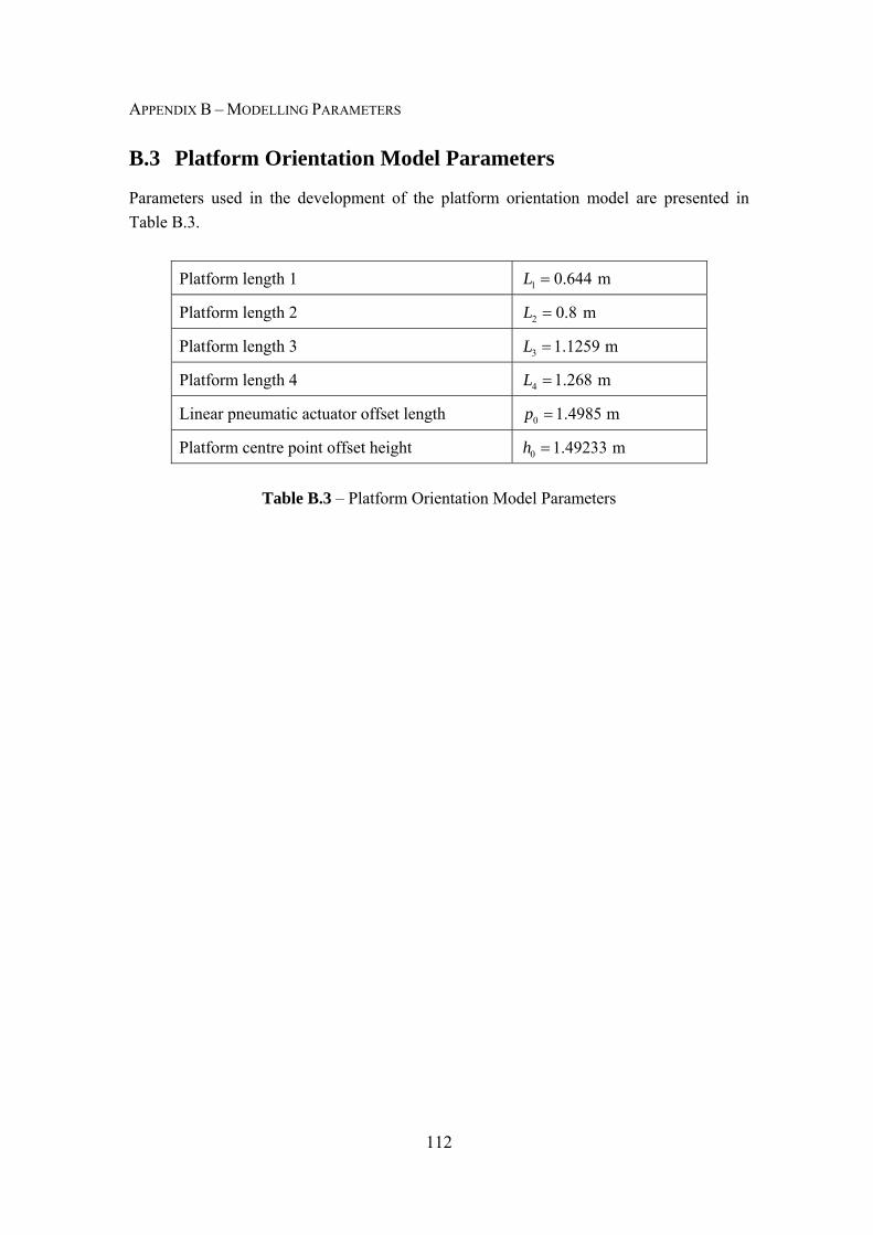
APPENDIX B – MODELLING PARAMETERS

112

B.3 Platform Orientation Model Parameters

Parameters used in the development of the platform orientation model are presented in Table B.3.

Platform length 1 1 0.644L = m




Linear pneumatic actuator offset length 0 1.4985p = m

Platform centre point offset height 0 1.49233h = m

Table B.3 – Platform Orientation Model Parameters

113

Ship Centreline

RPΘ

RPΦ

Recording Point

Flight Deck Centre

Appendix C

Ship Motion Data In this appendix, details of the ship motion data obtained are presented. These details include information on the ship’s axis system as well as an overview of the actual ship motions.

C.1 Ship Axis System

An overview of the ship’s axis system, including details of the recording point and flight deck centre, is shown in Figure C.1.

Figure C.1 – Ship Axis System

x-axis z-axis

y-axis

ox

oy

oz

RPH

FDH

APPENDIX C – SHIP MOTION DATA

114

Details of the ship’s axis system and position offsets are listed in Table C.1 and Table C.2 respectively.

Axis

Name Measured from Orientation (Right Hand Rule)

Flight Deck Centre

INS1 (IMT Recording Point)

x Bow Pointing to the stern 102.6 m 44.25 m

y Centreline Pointing starboard 0 m 0.525 m

z Design Waterline Pointing up 9.7 m 1.925 m

Table C.1 – Details of the Ship’s Axis System

Axis Position offset

x-axis, ox 58.35 m

y-axis, oy 0.525 m

z-axis, oz 7.775 m

Table C.2 – Position Offsets

C.2 Ship Motion Data

The heading, heave, pitch and roll motions for the 10 minutes of motion data obtained, relating to one of the South African Navy Patrol Corvettes, are shown in Figure C.2 to Figure C.9. The transformed flight deck heave and heave rate are also shown in Figure C.10 and Figure C.11 respectively.

0 100 200 300 400 500 6000

50

100

150

200

250

300

350

Hea

ding

[deg

]

Time [s] Figure C.2 – Recording Point Heading


115

0 100 200 300 400 500 600-2

-1.5

-1

-0.5

0

0.5

1

Hea

ding

Rat

e [d

eg/s

]

Time [s] Figure C.3 – Recording Point Heading Rate

0 100 200 300 400 500 600-2.5

-2

-1.5

-1

-0.5

0

0.5

1

1.5

2

2.5

Hea

ve [m

]

Time [s] Figure C.4 – Recording Point Heave

0 100 200 300 400 500 600-1.5

-1

-0.5

0

0.5

1

1.5

2

Hea

ve R

ate

[m/s

]

Time [s] Figure C.5 – Recording Point Heave Rate

0 100 200 300 400 500 600-3

-2

-1

0

1

2

3

Pitc

h [d

eg]

Time [s] Figure C.6 – Recording Point Pitch


116

0 100 200 300 400 500 600-2.5

-2

-1.5

-1

-0.5

0

0.5

1

1.5

2

2.5

Pitc

h R

ate

[deg

/s]

Time [s] Figure C.7 – Recording Point Pitch Rate

0 100 200 300 400 500 600-6

-4

-2

0

2

4

6

8

Rol

l [de

g]

Time [s] Figure C.8 – Recording Point Roll

0 100 200 300 400 500 600-5

-4

-3

-2

-1

0

1

2

3

4

5

Rol

l Rat

e [d

eg/s

]

Time [s] Figure C.9 – Recording Point Roll Rate

0 100 200 300 400 500 600-5

-4

-3

-2

-1

0

1

2

3

4

5

Flig

ht D

eck

Hea

ve [m

]

Time [s] Figure C.10 – Transformed Flight Deck Heave


117

0 100 200 300 400 500 600-4

-3

-2

-1

0

1

2

3

4

Flig

ht D

eck

Hea

ve R

ate

[m/s

]

Time [s] Figure C.11 – Transformed Flight Deck Heave Rate

118

Bibliography

[1] E. Richer, Y. Hurmuzlu. A High Performance Pneumatic Force Actuator System,

Part 1 – Nonlinear Mathematical Model. ASME Journal of Dynamic Systems, Measurement and Control, Vol. 122, No.3, pp. 416-425, 2000.

[2] Ž. Šitum, J. Petrić. Modeling and Control of Servopneumatic Drive. Strojarstvo 43

(1-3), pp. 29-39, 2001. [3] Ž. Šitum, B. Novaković, J. Petrić. Identification and Control of Pneumatic

Servodrives. The 9th Mediterranean Conference on Control and Automation, 2001. [4] H. Olsson, K.J. Åström, C. Canudas de Wit, M. Gäfvert, P. Lischinsky. Friction

Models and Friction Compensation. European J. of Control, 4(3), pp. 176-195, 1998.

[5] C.T. Crowe, D.F. Elger, J.A. Roberson. Engineering Fluid Mechanics, Seventh

Edition. McGraw – Hill, 2001. [6] Ž. Šitum, J. Petrić, M. Crneković. Sliding Mode Control Applied to Pneumatic

Servo Drive. Proceedings of 11th Mediterranean Conference on Control and Automation, 2003.

[7] J.J. Slotine, W. Li. Applied Nonlinear Control. Prentice-Hall, 1991. [8] B.W. Surgenor, N.D. Vaughan. Continuous Sliding Mode Control of a Pneumatic

Actuator. ASME Journal of Dynamic Systems, Measurement and Control, Vol. 119, pp. 578-581, 1997.

BIBLIOGRAPHY

119

[9] E. Richer, Y. Hurmuzlu. A High Performance Pneumatic Force Actuator System, Part 2 – Nonlinear Controller Design. ASME Journal of Dynamic Systems, Measurement and Control, Vol. 122, No. 3, pp. 426-434, 2000.

[10] J. Diebel. Representing Attitude: Euler Angles, Unit Quaternions and Rotation

Vector. Stanford University, 2006. [11] I.K. Peddle. Autonomous Flight of a Model Aircraft. Masters thesis, Stellenbosch

University, April 2005. [12] D.R. Gaum. Aggressive Flight Control Techniques for a Fixed Wing Unmanned

Aerial Vehicle. Masters thesis, Stellenbosch University, March 2009. [13] J. Penny, G. Lindfield. Numerical Methods using Matlab, Second Edition. Prentice-

Hall, 2000. [14] R. Busch. Modelling and simulation of an autonomous underwater vehicle. Masters

thesis, Stellenbosch University, March 2009. [15] D.R. Gaum. Revised OpenGL Graphical Simulator. Stellenbosch University, 2009. [16] J.D. Loy. Corvette 3D Model. Stellenbosch University, 2009. [17] J.G. Proakis, D.G. Manolakis. Digital Signal Processing, Third Edition. Prentice-

Hall, 1996. [18] DOD Dictionary web page. http://www.dtic.mil/doctrine/jel/doddict. 2009. [19] Teal Group Corporation web page. http://www.tealgroup.com. 2009. [20] L.A. Ingham. Considerations for a roadmap for the operation of unmanned aerial

vehicles (UAV) in South African airspace. PhD dissertation, Stellenbosch University, 2008.

[21] A.M. De Jager. Redundant Inertial Navigation and High Accuracy Visual-based

State Estimation for Autonomous Rotary Wing Landing. Masters Thesis, Stellenbosch University, To be Submitted.

BIBLIOGRAPHY

120

[22] J.D. Loy. Aggressive helicopter flight and autonomous landing of an unmanned helicopter on a moving platform. Masters Thesis, Stellenbosch University, To be Submitted.

[23] F.N. Alberts. Autonomous Landing of a Fixed-wing Unmanned Aerial Vehicle on a

Moving Platform. Masters Thesis, Stellenbosch University, To be Submitted. [24] The South African Navy & Marine and Coastal Management web page.

http://navy.org.za/pages/valour. 2009. [25] InMotion Simulation web page. http://www.inmotionsimulation.com. 2009. [26] R. Eschmann. Modellbildung und Simulation pneumatischer Zylinderantriebe.

PHD thesis, RWTH Aachen, 1994. [27] A.H. Basson, T.W. von Backström. Guide for Writing Technical Reports, Second

Edition. Stellenbosch University, 2003. [28] J. Iovine. PIC Microcontroller Project Book. McGraw-Hill, 2000. [29] D.A. Neamen. Electronic Circuit Analysis and Design, Second Edition. McGraw- Hill, 2001. [30] D.G. Ullman. The Mechanical Design Process, Third Edition. McGraw – Hill,

2003. [31] R. Craig. Mechanics of Materials, Second Edition. John Wiley & Sons, 2000. [32] E. Shingly. Mechanical Engineering Design, Seventh Edition. McGraw – Hill,

2003. [33] S. Chapman. MATLAB Programming for Engineers, Second Edition. Brooks/Colel,

2003. [34] G.F. Franklin, J.D. Powell, A. Emami-Naeini. Feedback Control of Dynamic

Systems, Fourth Edition. Prentice-Hall, 2002. [35] C.M. Close, D.K. Frederick, J.C. Newell. Modeling and Analysis of Dynamic

Systems, Third Edition. John Wiley & Sons, 2002.

BIBLIOGRAPHY

121

[36] G.F. Franklin, J.D. Powell, M.L. Workman. Digital Control of Dynamic Systems, Third Edition. Addison Wesley Longman, 1998.

[37] W. Bolton. Mechatronics, Third Edition. Prentice-Hall, 2003. [38] M. Guillon. Hydraulic Servo Systems. Butterworth & Co, 1969. [39] C.R. Burrows. Fluid Power Servomechanisms. Butler & Tanner, 1972. [40] C.A. Belsterling. Fluidic Systems Design. John Wiley & Sons, 1971. [41] D. Bouteille. Fluid Logic Controls and Industrial Automation. John Wiley & Sons,

1973. [42] W. Bolton. Control Engineering, Third Edition. Addison Wesley Longman, 1998. [43] C. Edwards, S.K. Spureon. Sliding Mode Control: Theory and Applications. Taylor

& Francis, 1998. [44] S.R. Pandian, F. Takemura, Y. Hayakawa, S. Kawamura. Pressure Observer-

Controller Design for Pneumatic Cylinder Actuators. IEEE/ASME Transactions on Mechatronics, Vol. 7, No. 4, pp. 490-499, 2002.

[45] J. Wang, J. Pu, P. Moore. A practical control strategy for servo-pneumatic actuator

systems. Control Engineering Practice, Vol. 7, pp. 1483-1488, 1999. [46] F. Xiang, J. Wikander. Block-oriented approximate feedback linearization for

control of pneumatic actuator system. Control Engineering Practice, Vol. 12, pp. 387-399, 2004.

[47] T. Kimura, S. Hara, T. Fujita, T. Kagawa. Feedback linearization for pneumatic

actuator systems with static friction. Control Engineering Practice, Vol. 5, No. 10, pp. 1385-1394, 2000.

[48] Y.S. Jeon, C.O. Lee, Y.S. Hong. Optimization of the control parameters of a

pneumatic servo cylinder drive using genetic algorithms. Control Engineering Practice, Vol. 6, pp. 847-853, 1998.

BIBLIOGRAPHY

122

[49] F. Xiang, J. Wikander. QFT control design for an approximately linearized pneumatic positioning system. International Journal of Robust and Nonlinear Control, Vol. 13, pp. 675-688, 2003.

[50] A.R.W. Huang, C. Chen. A Low-Cost Driving Simulator for Full Vehicle Dynamics Simulation. IEEE Transactions on Vehicular Technology, Vol. 52, No. 1,

pp. 162-172, 2003. [51] IMT web page. http://www.armscorbusiness.com/SubSites/IMT/IMT03_landing.

2009. [52] Armscor web page. http://www.armscorbusiness.com/. 2009. [53] The South African Navy web page. http://www.navy.mil.za. 2009. [54] Motion Platforms web page. http://www.mfs.com.au/MFS_Motion_Platforms.

2009. [55] J.C. Roos. Autonomous Take-Off and Landing of a Fixed Wing Unmanned Aerial

Vehicle. Masters thesis, Stellenbosch University, March 2007. [56] W.J. Hough. Autonomous Aerobatic Flight of a Fixed Wing Unmanned Aerial

Vehicle. Masters thesis, Stellenbosch University, March 2007. [57] D. Blaauw. Control of a Variable Stability Aircraft. Masters Thesis, Stellenbosch

University, March 2009. [58] L.E. Rossouw. Autonomous Flight of an Unmanned Helicopter. Masters thesis, Stellenbosch University, March 2008. [59] C. Van Schalkwyk. Full State Control of a Fury X-Cell Unmanned Helicopter.

Masters Thesis, Stellenbosch University, March 2009. [60] B.J. Visser. The precision landing of an UAV. Masters Thesis, Stellenbosch

University, March 2009. [61] R.D. De Hart. Advanced Take-off and Flight Control Algorithms for Fixed Wind

Unmanned Aerial Vehicles. Masters Thesis, Stellenbosch University, To be Submitted.

development of a 3-dof motion simulation platform

Documents