EPRI Project Manager

Jeff Phillips

Advisors

David Thimsen

Adam Berger

Dale Grace

ELECTRIC POWER RESEARCH INSTITUTE 3420 Hillview Avenue, Palo Alto, California 94304-1338 PO Box 10412, Palo Alto, California 94303-0813 USA

800.313.3774 650.855.2121 askepri@epri.com www.epri.com

Development of a Brayton Bottoming Cycle using

Supercritical Carbon Dioxide as the Working Fluid

by

Grant Kimzey

A report submitted in partial fulfillment of the requirements for:

Gas Turbine Industrial Fellowship

University Turbine Systems Research Program

2

Table of Contents

Introduction……………………………………………………………………………………..2

Project Scope……………………………………………………………………………………4

Benchmarking…………………………………………………………………………………..4

Design Parameters, Constraints, and Assumptions……………………………………………..5

Initial Modeling and Analysis…………………………………………………………………..9

Sensible Heat vs. Heat Flux Sources…………………………………………………………...11

Proposed Cycles

Cycle 1…………………………………………………………………………………14

Cycle 2…………………………………………………………………………………17

Cycle 3…………………………………………………………………………………22

Effect of Intercooling on Cycle Performance………………………………………………….19

Summary of Results……………………………………………………………………………28

Conclusions and Recommendations…………………………………………………………...29

References………………………………………………………………………………………30

Acknowledgements…………………………………………………………………………….31

3

Introduction

Inherent in any power cycle is the ultimate rejection of a significant amount of thermal

energy, which exits the system either by heat transfer in a closed cycle, or via thermal transport

by exhaust gases in an open cycle. All heat that is rejected to the environment is heat that is not

being used to generate power, so needless to say, a significant amount of effort is made to make

as much use of this waste heat as possible. One method of recovering this waste heat is to

integrate a secondary, or bottoming cycle into the system that essentially uses the waste heat of

the primary, or topping cycle, as its heat source. The use of a bottoming cycle boosts the overall

plant efficiency, meaning that more usable power is generated using the same amount of fuel.

By far the most commonly encountered bottoming cycle today is the Rankine cycle,

using steam as the working fluid. The Rankine cycle is very well researched, and is used

worldwide, both in topping and bottoming cycle applications. Recently, however, a number of

research teams have begun to look for an alternative to the classic steam cycle, with a growing

focus on Brayton cycles using supercritical carbon dioxide (sCO2) as the working fluid.

Researchers claim that an sCO2 power cycle could potentially exhibit a higher thermal

efficiency than steam cycles when operating between the same maximum and minimum cycle

temperatures. In addition, the high energy density of sCO2 suggests that the size requirements

for the turbomachinery used in an sCO2 power cycle could potentially be much lower than those

used in steam cycle generation, which may result in lower capital costs.

As a result, a Brayton power cycle using sCO2 as the working fluid has the potential to

replace the Rankine cycle in both topping cycle and bottoming cycle applications. To date, most

research in the field has been dedicated to the use of sCO2 as the primary power cycle in nuclear

applications. Additional research is being conducted regarding the use of an sCO2 cycle in other

4

primary cycle applications, but relatively little research has been aimed toward developing an

sCO2 cycle that is well-suited to bottoming cycle applications.

Project Scope

The primary focus of this project at the start was to verify claims that an sCO2 Brayton

cycle would yield a marginally higher thermal efficiency than a Rankine steam cycle while

operating between the same minimum and maximum temperatures. Three commonly proposed

Brayton cycles were to be modeled and optimized, and their thermal efficiencies were to then be

compared to a Rankine steam cycle operating under the same conditions. As will be discussed,

the three proposed cycles turned out to be unsuitable for a bottoming cycle application, and were

scrapped. At this point, the project scope evolved to include designing and modeling new

potential cycle configurations, with the goal of creating a new cycle configuration that

maximizes both efficiency and waste heat recovery. In all, nearly thirty different cycle

configurations were conceived of, modeled, and evaluated. While most of these cycles turned out

to be unsuitable for further development, three of the modeled cycles showed enough potential to

be included in this report.

Benchmarking

In order to gauge the performance of each cycle configuration, two modern combined

cycles were selected as benchmarks. The two cycles chosen represent two opposite ends of a

broad spectrum of combined cycles, ranging from low power, low temperature applications to

high power, high temperature applications.

The first benchmark cycle is the Siemens H Class gas turbine. This cycle employs an

internal combustion turbine fueled by natural gas as the topping cycle, with a 3 pressure level,

5

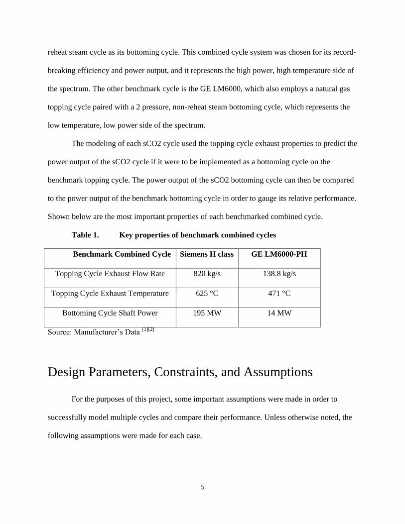
reheat steam cycle as its bottoming cycle. This combined cycle system was chosen for its record-

breaking efficiency and power output, and it represents the high power, high temperature side of

the spectrum. The other benchmark cycle is the GE LM6000, which also employs a natural gas

topping cycle paired with a 2 pressure, non-reheat steam bottoming cycle, which represents the

low temperature, low power side of the spectrum.

The modeling of each sCO2 cycle used the topping cycle exhaust properties to predict the

power output of the sCO2 cycle if it were to be implemented as a bottoming cycle on the

benchmark topping cycle. The power output of the sCO2 bottoming cycle can then be compared

to the power output of the benchmark bottoming cycle in order to gauge its relative performance.

Shown below are the most important properties of each benchmarked combined cycle.

Table 1. Key properties of benchmark combined cycles

Benchmark Combined Cycle Siemens H class GE LM6000-PH

Topping Cycle Exhaust Flow Rate 820 kg/s 138.8 kg/s

Topping Cycle Exhaust Temperature 625 °C 471 °C

Bottoming Cycle Shaft Power 195 MW 14 MW

Source: Manufacturer’s Data [1][2]

Design Parameters, Constraints, and Assumptions

For the purposes of this project, some important assumptions were made in order to

successfully model multiple cycles and compare their performance. Unless otherwise noted, the

following assumptions were made for each case.

6

Thermodynamic Fluid Properties

There are assumptions made in “textbook” calculations which cannot be justified while

analyzing sCO2 Brayton Cycles.

1. Ideal gas behavior

A real gas may be approximated as an ideal gas only at relatively low pressures and high

temperatures. Generally, it is an accurate assumption if

Where is the pressure at the critical point and is the temperature at the critical point

The cycles discussed in this report operate within the range of

36.9°C (310 K) <T< 604.9°C (878 K)

5000 kPa<P<27600 kPa

The critical point of CO2 is

304.19 K

7380 kPa

So the range of relative temperature and pressure is

which does not justify the use of the ideal gas assumption.

2. Constant specific heat capacity

Specific heat capacity is a very important property of gas, particularly when analyzing heat

transfer and power cycles. A common assumption is that the specific heat of a gas remains

constant through small changes in pressure and temperature. This assumption is not valid for a

supercritical fluid, which is shown graphically in Figure 1.

7

Figure 1. Specific heat capacity of sCO2 vs Temperature, calculated using NIST

REFPROP thermodynamic properties database

The heat capacity varies substantially with temperature and with pressure, meaning the

constant specific heat capacity assumption is invalid. Instead, fluid properties such as

temperature and enthalpy are calculated directly using the NIST Reference Fluid

Thermodynamic and Transport Properties Database (REFPROP) version 9.0.

Operating Constraints

For the purposes of this project, some operating conditions were imposed in order to keep

costs low and to create a realistic model. The maximum operating pressure is limited to 276 bar

0 100 200 300 400 500 600 7001000

1200

1400

1600

1800

2000

2200

Temperature(C)

Specific

Heat

Capacity (

J/k

g*K

)

P = 5000 kPa

P = 27600 kPa

8

(4000 PSI) in order to avoid using excessively thick piping and flanges. The maximum operating

temperature is limited by the exhaust temperature of the topping cycle. The maximum

temperature must be lower than the exhaust temperature by some temperature difference, which

was chosen as 20° C for this project. Finally, the minimum temperature (compressor inlet

temperature) is limited to 36.85° C.

Pressure Losses

In the idealized Brayton cycle, all heating and cooling occurs isobarically, meaning that

the pressure remains constant. Supercritical CO2 has a low viscosity, but nevertheless, pressure

losses in the flow still occur within the heat exchangers and recuperators, and need to be

accounted for while modeling evaluating the performance of a power cycle. In all of the

following analyses, a 0.5% loss in pressure was assumed through each heat exchanger and

through each recuperator.

Isentropic Efficiencies of Turbines and Compressors

For the idealized Brayton cycle, the working fluid is compressed and expanded

isentropically, meaning that the entropy of the working fluid remains constant throughout the

process. This will only occur if no heat is transferred to or from the working fluid during the

process, and if the process is completely reversible. Because of inherent irreversibilities in actual

processes, no real expansion or compression process is truly isentropic, so an assumed isentropic

efficiency is used to describe the relative performance of the compressors and turbines. This

analysis uses an assumed 85% isentropic compressor efficiency and an assumed 90% isentropic

turbine efficiency.

9

Recuperator and Heat Exchanger Constraints

A recuperator/heat exchanger can be constrained in one of two ways. The effectiveness

may be defined, which describes the quantity of heat transferred in relation to the maximum

possible quantity of heat transferred. The other way to constrain the system is by defining the

minimum terminal temperature difference, or TTD. In the interest of maintaining control over

the turbine inlet temperature(s), the TTD method was chosen. A low TTD corresponds to a high

recuperator effectiveness, and a high recuperator effectiveness generally corresponds to a more

efficient power-cycle. A conflict arises, however, because the cost of a highly effective

recuperator is a much greater than the cost of a less effective recuperator. To keep costs within

reason, all TTDs were chosen to be 20° C in this report.

Additional Assumptions

The system is assumed to be in steady-state operation. The following analysis does not

include information regarding performance while the cycle is ramping up or ramping down. The

system is assumed to be adiabatic, with no heat being lost to the surroundings, other than from

the precooler or intercooler if applicable.

Initial Modeling and Analysis

At the start of this project, three proposed bottoming cycles were modeled, using the

maximum exhaust temperature of the Siemens H class minus the appropriate TTD (20°C) as the

maximum cycle temperature. All modeling efforts utilized MATLAB software, which accessed

the NIST Reference Fluid Thermodynamic and Transport Properties Database (REFPROP) for

10

all thermodynamic properties, and made the necessary calculations in order to predict the

operating conditions and performance of each sCO2 cycle. Shown below are the three cycles

modeled initially, along with their optimized thermal efficiency.

Figure 2. Simple Recuperated Cycle Flowsheet

Figure 3. Recuperated Recompression Cycle Flowsheet

Recuperators

Qin

Cooler

Main compressor Turbine

Qout

1

2

4

5

6

8

Heater

Recompressor

3

7

Recuperator

Qin

Cooler

Compressor Turbine

Qout

1

2

4

5

6

8

Heater

Simple Recuperated Cycle

Thermal Efficiency = 40.3%

Recuperated Cycle with Recompression

Thermal Efficiency = 45.4%

11

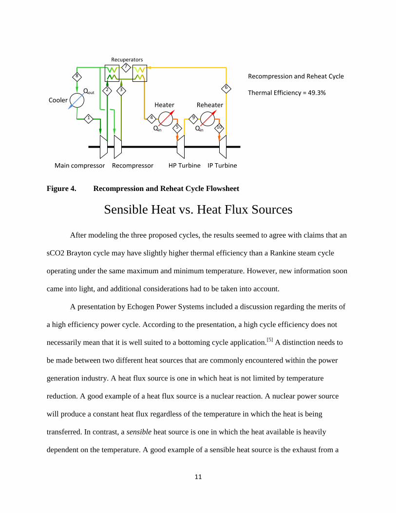
Figure 4. Recompression and Reheat Cycle Flowsheet

Sensible Heat vs. Heat Flux Sources

After modeling the three proposed cycles, the results seemed to agree with claims that an

sCO2 Brayton cycle may have slightly higher thermal efficiency than a Rankine steam cycle

operating under the same maximum and minimum temperature. However, new information soon

came into light, and additional considerations had to be taken into account.

A presentation by Echogen Power Systems included a discussion regarding the merits of

a high efficiency power cycle. According to the presentation, a high cycle efficiency does not

necessarily mean that it is well suited to a bottoming cycle application.[5]

A distinction needs to

be made between two different heat sources that are commonly encountered within the power

generation industry. A heat flux source is one in which heat is not limited by temperature

reduction. A good example of a heat flux source is a nuclear reaction. A nuclear power source

will produce a constant heat flux regardless of the temperature in which the heat is being

transferred. In contrast, a sensible heat source is one in which the heat available is heavily

dependent on the temperature. A good example of a sensible heat source is the exhaust from a

Qin

Recuperators

Qin

Cooler

Main compressor HP Turbine

Qout

1

2

4 9

8

Heater

Recompressor

3

7

IP Turbine

Reheater

6

10 5

Recompression and Reheat Cycle

Thermal Efficiency = 49.3%

12

combustion cycle. The heat available from a sensible heat source is roughly proportional to its

temperature change, that is . A consequence of this property is

that only a small portion of the available waste heat is recoverable at high temperatures. The

commonly proposed cycles shown above are well suited to operating with a heat flux producing

power source, but are not well suited to a sensible heat source, such as topping cycle exhaust.

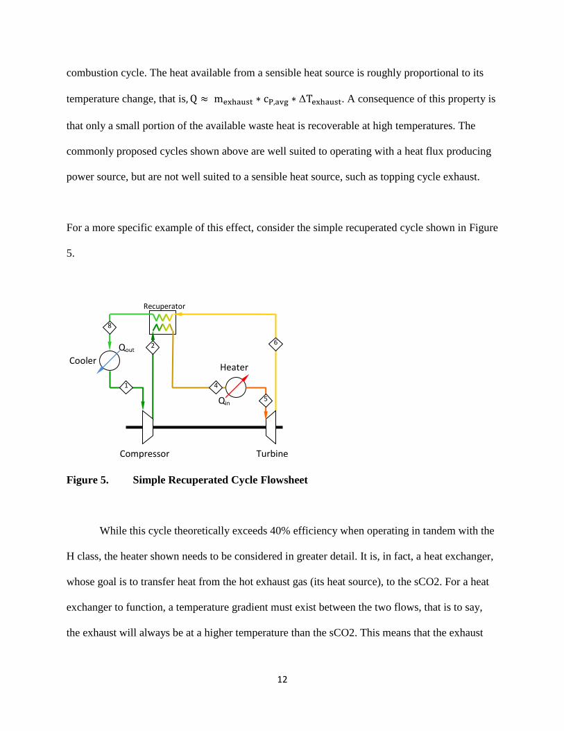
For a more specific example of this effect, consider the simple recuperated cycle shown in Figure

5.

Figure 5. Simple Recuperated Cycle Flowsheet

While this cycle theoretically exceeds 40% efficiency when operating in tandem with the

H class, the heater shown needs to be considered in greater detail. It is, in fact, a heat exchanger,

whose goal is to transfer heat from the hot exhaust gas (its heat source), to the sCO2. For a heat

exchanger to function, a temperature gradient must exist between the two flows, that is to say,

the exhaust will always be at a higher temperature than the sCO2. This means that the exhaust

Recuperator

Qin

Cooler

Compressor Turbine

Qout

1

2

4

5

6

8

Heater

13

gases will only supply heat until it reaches a temperature marginally greater than . Due to the

recuperator, is considerably higher than the ambient temperature, in the vicinity of 400° C,

which means that the exhaust gases, which are this cycle’s heat source, will only be cooled to

perhaps 420° C. This 420 degree exhaust can no longer supply any heat to the system, so it exits,

carrying with it a significant portion of its initial thermal energy. From its initial temperature of

625° C, the exhaust has only been cooled by 205°C. If instead this exhaust were cooled to say,

215° C, the temperature change has doubled, which means that the heat input to the system has

roughly doubled.

To put it another way, a bottoming cycle may have a thermal efficiency of 50%, but if

only 100 MW of heat is supplied to the system, the cycle will only produce 50 MW of usable

power. On the other hand, another power cycle might have a thermal efficiency of only 30%, but

if it can recover 300 MW of heat from the exhaust, it will produce 90 MW of usable power,

nearly double the power of the first cycle. So, while thermal efficiency is certainly an important

quality of any power cycle, a high cycle efficiency does not necessarily correlate with a high

power output when used with a sensible heat source. A truly effective bottoming cycle would be

one in which thermal efficiency is balanced with the ability to recover waste heat. For this

reason, in the remainder of this report, the power output of each cycle will be used as the primary

measure of each cycle’s performance.

14

Baseline Cascade Cycle (Cycle 1) Modeling

Included in the Echogen presentation was a simple, baseline idea for an sCO2 bottoming cycle.

Figure 6. Cycle 1 Flowsheet

The cycle consists of one compressor that supplies all of the high pressure, low

temperature CO2. The compressor outlet stream is split into two separate flows. The first stream

travels through the heat exchanger, recovering heat from the topping cycle exhaust. This first

stream is expanded in turbine 1, and is then used to heat the other stream, which is expanded in

turbine 2. The advantage of this configuration is that it recovers a large portion of the waste heat

from the topping cycle. Due to the absence of a recuperator on the first stream, the exhaust

reaches a temperature marginally above , which is far lower than from the previous case. A

m1

m2

Low T

recuperator

High T

recuperator

15

much larger portion of the topping cycle waste heat is recovered, at the cost of thermal

efficiency. Shown below are the optimized cycle conditions for the H Class and LM6000 cases.

Also shown is the shaft power and efficiency of each cycle.

Table 2. Cycle 1 on H Class, state properties

State 1 2 3 4 5 6 7 8

Pressure(Bar) 85.00 276.00 274.62 85.86 85.43 85.43 274.62 273.25

Temperature (°C) 36.85 86.37 604.85 461.25 313.72 173.67 292.73 441.25

Enthalpy(kJ/kg) 332.12 367.96 1099.63 938.23 767.19 607.23 704.70 893.76

Entropy(kJ/kg*K) 1.4258 1.4408 2.7543 2.7790 2.5201 2.2085 2.1980 2.4958

m1 = 52.5% m2 = 47.5%

Power Output=133 MW

Efficiency = 28.38%

Table 3. Cycle 1 on LM6000, state properties

State 1 2 3 4 5 6 7 8

Pressure(Bar) 85.00 276.00 274.62 85.86 85.43 85.43 274.62 273.25

Temperature (°C) 36.85 86.37 450.85 322.38 187.64 129.01 167.51 302.38

Enthalpy(kJ/kg) 332.12 367.96 905.68 776.99 623.45 553.61 525.26 717.53

Entropy(kJ/kg*K) 1.4258 1.4408 2.5115 2.5357 2.2443 2.0820 1.8378 2.2214

m1 = 55.6% m2 = 44.4%

16

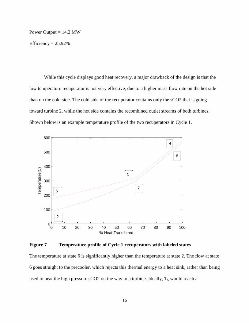
Power Output = 14.2 MW

Efficiency = 25.92%

While this cycle displays good heat recovery, a major drawback of the design is that the

low temperature recuperator is not very effective, due to a higher mass flow rate on the hot side

than on the cold side. The cold side of the recuperator contains only the sCO2 that is going

toward turbine 2, while the hot side contains the recombined outlet streams of both turbines.

Shown below is an example temperature profile of the two recuperators in Cycle 1.

Figure 7 Temperature profile of Cycle 1 recuperators with labeled states

The temperature at state 6 is significantly higher than the temperature at state 2. The flow at state

6 goes straight to the precooler, which rejects this thermal energy to a heat sink, rather than being

used to heat the high pressure sCO2 on the way to a turbine. Ideally, would reach a

0 10 20 30 40 50 60 70 80 90 1000

100

200

300

400

500

600

% Heat Transferred

Tem

pera

ture

(C)

8

4

5

7

2

6

17

temperature only marginally above , which would signify that a larger quantity of heat was

recuperated.

Cycle 2

In an effort to reduce the heat rejection in the precooler, I devised another cycle

configuration that allows for a slightly higher flow rate through the cool side of the low

temperature recuperator. The higher flow rate causes a slightly larger amount of heat to be

recuperated from the turbine outlet streams.

Figure 8 Cycle 2 Flowsheet

The main difference from Cycle 1 is that the hot exhaust gas is used to heat the high

pressure sCO2 on the way to both turbines. The hot exhaust gas is first used to heat stream 2

from to , then to heat stream 1 from to . This configuration allows for the mass

flowrate through the cold side of the low temperature recuperator to be slightly higher, causing

the temperature profile to track a little bit more closely.

m2 m1

18

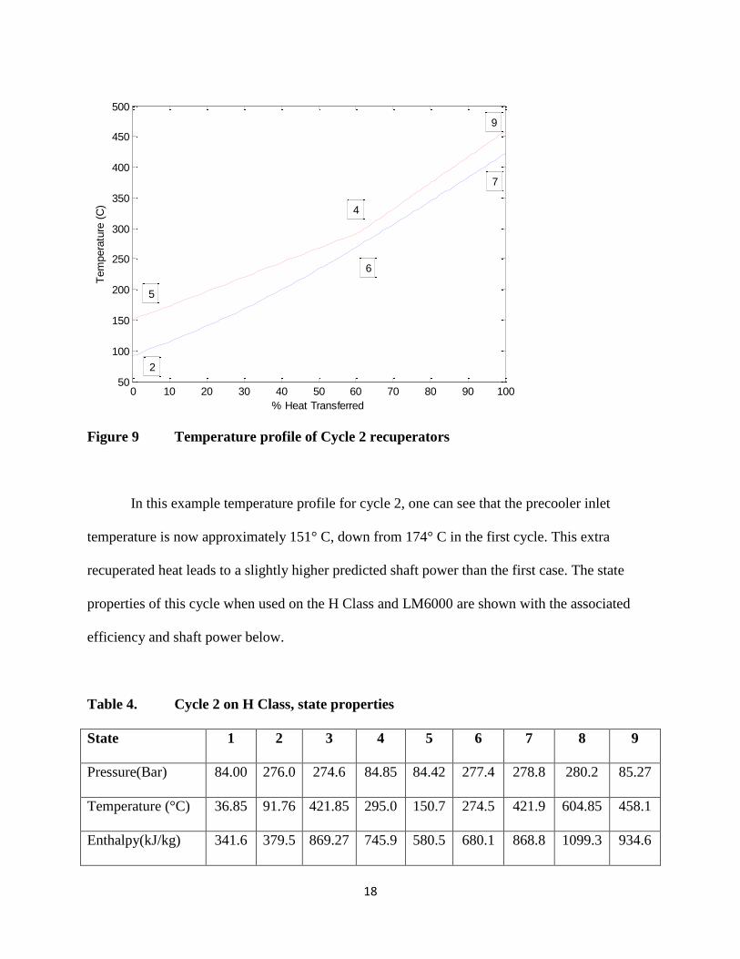
Figure 9 Temperature profile of Cycle 2 recuperators

In this example temperature profile for cycle 2, one can see that the precooler inlet

temperature is now approximately 151° C, down from 174° C in the first cycle. This extra

recuperated heat leads to a slightly higher predicted shaft power than the first case. The state

properties of this cycle when used on the H Class and LM6000 are shown with the associated

efficiency and shaft power below.

Table 4. Cycle 2 on H Class, state properties

State 1 2 3 4 5 6 7 8 9

Pressure(Bar) 84.00 276.0 274.6 84.85 84.42 277.4 278.8 280.2 85.27

Temperature (°C) 36.85 91.76 421.85 295.0 150.7 274.5 421.9 604.85 458.1

Enthalpy(kJ/kg) 341.6 379.5 869.27 745.9 580.5 680.1 868.8 1099.3 934.6

0 10 20 30 40 50 60 70 80 90 10050

100

150

200

250

300

350

400

450

500

% Heat Transferred

Tem

pera

ture

(C

)

5

4

9

2

6

7

19

Entropy(kJ/kg*K) 1.457 1.472 2.4601 2.489 2.149 2.152 2.457 2.750 2.775

m1=45% m2=55%

Power = 145 MW

Efficiency = 31.18%

Table 5. Cycle 2 on LM6000, state properties

State 1 2 3 4 5 6 7 8 9

Pressure(Bar) 84.00 276.0 274.6 84.85 84.42 277.4 278.8 280.2 85.27

Temperature (°C) 36.85 91.76 246.9 136.5 117.6 116.8 246.9 451.2 319.8

Enthalpy(J/kg) 341.6 379.5 643.3 563.2 539.8 431.5 642.5 905.6 774.2

Entropy(J/kg*K) 1.457 1.473 2.085 2.107 2.049 1.610 2.081 2.507 2.532

m1=55% m2=45%

Efficiency = 24.78%

Power = 13.4 MW

Effect of Intercooling on Cycle Performance

Adding an intercooler to the compression process was found to increase the net power

output of the previous two cycles. The intercooler decreases the total compression work, and it

also decreases the minimum temperature of the high pressure sCO2. The lower temperature at

the compressor outlet increases the heat transfer in the low temperature recuperator, and also

cools the topping cycle exhaust gases to a lower temperature, improving the ability of the cycle

to recover heat from the topping cycle exhaust gases.

20

Figure 10. Cycle 1 with intercooler flowsheet

Table 6. Intercooled Cycle 1 on H Class, state properties

State 1 2 3 4 5 6 7 8 9 10 11

Pressure(Bar) 60.00 89.00 88.56 276.0 274.6 60.60 60.30 274.6 273.3 271.9 60.91

Temperature (°C) 36.85 69.72 36.85 76.62 370.9 218.1 102.9 197.7 370.8 604.8 424.7

Enthalpy(kJ/kg) 445.7 464.6 314.9 347.1 805.0 666.6 537.9 572.9 805.2 1099. 898.8

Entropy(kJ/kg*K) 1.8270 1.8353 1.3681 1.3820 2.3641 2.3958 2.0976 1.9425 2.3653 2.7564 2.789

m1 = 43% m2 = 57%

Power = 161 MW

Efficiency = 33.71 %

21

Table 7. Intercooled Cycle 1 on LM6000, state properties

State 1 2 3 4 5 6 7 8 9 10

Pressure(Bar) 50.00 89.00 88.56 276.0 274.6 50.76 50.50 50.25 274.6 273.3

Temperature (°C) 36.85 86.90 36.85 76.62 450.9 272.0 99.17 98.12 77.75 252.0

Enthalpy(J/kg) 462.4 493.6 314.8 347.1 905.7 728.6 540.3 539.3 349.7 650.7

Entropy(J/kg*K) 1.905 1.918 1.368 1.3820 2.5115 2.5481 2.1331 2.1312 1.390 2.099

m1 = 61.5% m2 = 38.5%

Power = 14.4 MW

Efficiency = 25.60%

Figure 11. Cycle 2 with intercooler flowsheet

Table 8. Intercooled Cycle 2 on H class, state properties

State 1 2 3 4 5 6 7 8 9 10 11

Pressure(Bar) 60.00 89.00 88.56 276.0 274.6 60.60 60.30 274.6 273.3 271.9 60.91

22

Temperature

(°C)

36.85 69.72 36.85 76.62 370.8 218.1 102.9 197.7 370.9 604.9 424.7

Enthalpy(kJ/kg) 445.7 464.6 314.9 347.1 805.0 666.6 537.9 572.9 805.1 1100. 898.8

Entropy

(kJ/kg*K)

1.827 1.835 1.368 1.382 2.364 2.396 2.098 1.943 2.365 2.756 2.789

m1 = 43% m2 = 57%

Power = 161 MW

Efficiency = 33.71 %

The addition of an intercooler into these cycles increases the net power significantly. The

power output of Cycle 1 increased by 12% on the H Class and 1.4% on the LM-6000. The power

output of Cycle 2 increased by 11% and 10% on the H Class and LM-6000 respectively. This

data suggests that the use of an intercooler should be considered for any sCO2 cycle.

Cycle 3

On Cycle 1 and Cycle 2, the recuperator temperature profiles still did not track very well,

so I decided to use a different approach for the last cycle. By studying a graph of the specific

heat capacity of high pressure sCO2, low pressure sCO2, and exhaust gas, I noticed that high

pressure sCO2 has a very large heat capacity at lower temperatures, which drops off as the

temperature rises. The low pressure sCO2 also has a higher heat capacity at low temperatures,

but it does not change as drastically.

23

Figure 12. Specific Heat Capacity vs Temperature

Using this graph, I designed a new cycle that takes advantage of this varying heat capacity by

controlling the sCO2 flow rates through the heat exchangers to maximize heat transfer.

24

Figure 13. Cycle 3 flowsheet

To understand this cycle, consider the hot exhaust gases from the topping cycle and the

turbine outlet streams to be two separate sources of heat for the high pressure sCO2 as it travels

toward the turbines. In the transition from state 4 to state 5, the high pressure sCO2 is heated

concurrently by either the external heat source (exhaust gases), or by recuperation. The flows are

recombined at state 5, and then split again, this time with different mass flow rates. The flow into

turbine 1 is heated by the exhaust gas, and the turbine 1 outlet stream is used to heat the turbine 2

inlet stream, just like in Cycle 1. The advantage of this configuration is the ability to “tune” the

temperature profiles of the recuperators by altering the mass flow rates through each recuperator

and heat exchanger. In this configuration, m2 should be larger than m1. A large m2, combined

1

4 5

6 7

8

9

10

3 2 m1

m2

m3

m4

T1

T2

m3 m3+m4

Hot Exhaust Gases

from Topping Cycle

25

with the high heat capacity of the high pressure, low temperature stream allows the temperature

profile of the low T recuperator profile to track very closely.

The flows are recombined at state 5, then split again, this time sending a higher ratio of

the sCO2 to be heated by the exhaust gases. By finding the optimal mass flow rates, the

temperature profiles of both recuperators can be more precisely controlled, ultimately leading to

a larger quantity of recuperated heat, without compromising the cycle’s ability to recover waste

heat from the topping cycle.

Shown is an example temperature profile of Cycle 3

Figure 14. Temperature profile for Cycle 3 recuperators

As can be seen, the temperature profile of both recuperators track much more closely

than in Cycles 1 or 2, and the precooler inlet temperature approaches the minimum temperature

0 20 40 60 80 10050

100

150

200

250

300

350

400

450

% Heat Transferred

Tem

pera

ture

(C

)

8

9

7

4

5

10

26

difference from the compressor outlet temperature, signifying that the quantity of recuperated

heat cannot be increased much further.

Table 9. Cycle 3 on H Class, state properties

m1 = 37% m2 = 63%

m3 = 55% m4= 45%

Power = 169 MW

Efficiency = 35.20%

State 1 2 3 4 5 6 7 8 9 10

Temp(°C) 36.85 70.69 36.85 75.08 232.28 604.85 424.14 247.92 90.98 404.10

Pressure(bar) 50.00 89.00 88.56 276.00 274.62 273.25 50.76 50.50 50.25 27324.69

Enthalpy(kJ/kg) 462.41 492.22 314.87 345.64 565.03 1099.69 877.53 666.54 528.32 822.91

Entropy(kJ/kg*K) 1.9049 1.9141 1.3681 1.3778 1.9257 2.7554 2.7924 2.4287 2.1014 2.3925

27

Table 10. Cycle 3 on LM6000, state properties

State 1 2 3 4 5 6 7 8 9 10

Pressure(Bar) 60.00 89.00 88.56 276.0 274.6 273.3 60.91 60.60 60.30 273.3

Temperature (°C) 36.85 69.72 36.85 76.62 105.0 451.1 289.7 129.1 98.55 269.7

Enthalpy(kJ/kg) 445.7 464.6 314.9 347.1 407.9 906.1 745.7 567.9 532.7 674.5

Entropy(kJ/kg*K) 1.827 1.835 1.368 1.382 1.550 2.513 2.545 2.174 2.084 2.144

m1 = 42% m2 = 58%

m3 = 60% m4 = 40%

Power = 15.2 MW

Efficiency = 27%

28

Summary of Results

The resultant power outputs of each sCO2 cycle when used with either the Siemens H

Class topping cycle or LM6000 topping cycle are tabulated in Table 11, along with the

benchmark steam bottoming cycle, found in bold at the bottom of the table.

Table 11. Summary of Power Output for all Cycles

H Class LM6000

Cycle 1 Power 133 MW 14.2 MW

Intercooled Cycle 1 Power 149 MW 14.4 MW

Cycle 2 Power 145 MW 13.4 MW

Intercooled Cycle 2 Power 161 MW 14.8 MW

Intercooled Cycle 3 Power 169 MW 15.2 MW

Current Steam Bottoming Cycle Power 195 MW 14.0 MW

For the H Class application, none of the proposed cycles meet the power output of the

steam cycle currently in use. In contrast, all of the sCO2 cycles have a higher output than the

steam cycle when used on the LM6000, save for the non-intercooled Cycle 2. The use of an

intercooler in each cycle increases the power output of the cycle for both the H Class and

LM6000 application. In both the LM6000 and H Class cases, Cycle 3 produces the highest

power output.

29

Conclusions and Recommendations

On the LM6000, the top performing cycle, Cycle 3, yields a theoretical power output that

is 8.6% higher than the benchmarked steam bottoming cycle. On the other hand, none of the

cycles modeled for the high temperature, high power H Class application exceeded the power

output of its current steam cycle. Taking only power output into consideration, these findings

suggest that an sCO2 bottoming cycle may be better suited to low temperature applications.

A more thorough analysis of these configurations, however, should also include a cost-

benefit analysis, in order to better gauge the advantages and disadvantages of an sCO2 cycle in

comparison to the standard Rankine steam cycle. While the highest performing sCO2 cycle

prediction yields only 86.7% of the power output of the current bottoming cycle in place on the

H Class, it may still be an attractive alternative, depending on the capital and maintenance costs

associated with its implementation. Cycle 3 is recommended for further research, as well as a

cost-benefit analysis regarding its potential use as a bottoming cycle for high power, high

exhaust temperature gas turbines.

The choice of recommended cycle configuration is not as straightforward for a low

power, low temperature application. In the high power case, the associated complexity and cost

of Cycle 3 in comparison to Cycles 1 and 2 is probably justified for the increased power output.

The comparison is not so simple in the other application. The difference in power between Cycle

1 and Cycle 3 is on the order of 1 MW, which may not be enough to justify the added complexity

of Cycle 3 in comparison to Cycle 1. All 3 cycles are recommended for further research and a

cost-benefit analysis with regard to its potential use as a bottoming cycle in low power, low

temperature applications.

30

Anyone involved in researching or developing an sCO2 bottoming cycle should be wary

of using cycle efficiency to describe the performance of a cycle configuration. Bottoming cycle

performance should be compared in the context of power output, rather than efficiency, because

bottoming cycles operate using a sensible heat source. The ideal sCO2 bottoming cycle will

correctly balance the importance of a high thermal efficiency with the ability of the cycle to

recover the maximum amount of heat from its source.

References

1. Siemens H Class Technical Data, http://www.energy.siemens.com/hq/en/power-

generation/gas-turbines/sgt5-8000h.htm#content=Technical%20Data

2. General Electric GE LM6000 Technical Data, http://www.ge-

energy.com/products_and_services/products/gas_turbines_aeroderivative/lm6000_ph.jsp

3. Modified Brayton Power Cycle Using Supercritical CO2 as the working fluid, EPRI

Internal Report

4. Thimsen, David. Coal Fleet Advisor Meeting, Scottsdale, AZ. “Closed Brayton Power

Cycle with Supercritical CO2 (SCO2) as Working Fluid”

5. Echogen Power Systems. EPS IGTI Gas Turbo Expo. “CO2 Power Cycle Developments

and Commercialization”. June 12, 2012.

31

Acknowledgements

I would like to thank Jeff Phillips for his unwavering support throughout this project, and for

encouraging me to go above and beyond the original project scope.

I would also like to thank David Thimsen for always being readily available with advice and

recommendations which led me to success in this project.

Last, I would like to thank Adam Berger for his help in getting me acquainted with EPRI and for

his support of this project.