development of a design guideline for bridge pile
TRANSCRIPT

Portland State University Portland State University
PDXScholar PDXScholar
Dissertations and Theses Dissertations and Theses
Fall 1-11-2018
Development of a Design Guideline for Bridge Pile Development of a Design Guideline for Bridge Pile
Foundations Subjected to Liquefaction Induced Foundations Subjected to Liquefaction Induced
Lateral Spreading Lateral Spreading
Jonathan A. Nasr Portland State University
Follow this and additional works at: https://pdxscholar.library.pdx.edu/open_access_etds
Part of the Civil and Environmental Engineering Commons
Let us know how access to this document benefits you.
Recommended Citation Recommended Citation Nasr, Jonathan A., "Development of a Design Guideline for Bridge Pile Foundations Subjected to Liquefaction Induced Lateral Spreading" (2018). Dissertations and Theses. Paper 4160. https://doi.org/10.15760/etd.6048
This Thesis is brought to you for free and open access. It has been accepted for inclusion in Dissertations and Theses by an authorized administrator of PDXScholar. Please contact us if we can make this document more accessible: [email protected].

Development of a Design Guideline for Bridge Pile Foundations Subjected to
Liquefaction Induced Lateral Spreading
by
Jonathan A. Nasr
A thesis submitted in partial fulfillment of the requirements for the degree of
Master of Science in
Civil and Environmental Engineering
Thesis Committee: Arash Khosravifar, Chair
Franz Rad Thomas Schumacher
Portland State University 2017

© 2017 Jonathan A. Nasr

i
ABSTRACT
Effective-stress nonlinear dynamic analyses (NDA) were performed for piles in
liquefiable sloped ground to assess how inertia and liquefaction-induced lateral
spreading combine in long-duration vs. short-duration earthquakes. A parametric
study was performed using input motions from subduction and crustal
earthquakes covering a wide range of earthquake durations. The NDA results
were used to evaluate the accuracy of the equivalent static analysis (ESA)
recommended by Caltrans/ODOT for estimating pile demands. Finally, the NDA
results were used to develop new ESA methods to combine inertial and lateral
spreading loads for estimating elastic and inelastic pile demands.
The NDA results showed that pile demands increase in liquefied conditions
compared to nonliquefied conditions due to the interaction of inertia (from
superstructure) and kinematics (from liquefaction-induced lateral spreading).
Comparing pile demands estimated from ESA recommended by Caltrans/ODOT
with those computed from NDA showed that the guidelines by Caltrans/ODOT
(100% kinematic combined with 50% inertia) slightly underestimates demands for
subduction earthquakes with long durations. A revised ESA method was
developed to extend the application of the Caltrans/ODOT method to subduction
earthquakes. The inertia multiplier was back-calculated from the NDA results and
new multipliers were proposed: 100% Kinematic + 60% Inertia for crustal
earthquakes and 100% Kinematic + 75% Inertia for subduction earthquakes. The

ii
proposed ESA compared reasonably well against the NDA results for elastic
piles. The revised method also made it possible to estimate demands in piles that
performed well in the dynamic analyses but could not be analyzed using
Caltrans/ODOT method (i.e. inelastic piles that remained below Fult on the liq
pushover curve). However, it was observed that the pile demands became
unpredictable for cases where the pile head displacement exceeded the
displacement corresponding to the ultimate pushover force in liquefied
conditions. Nonlinear dynamic analysis is required for these cases to adequately
estimate pile demands.

iii
DEDICATION
To my loving family, whose support and encouragement made this possible

iv
ACKNOWLEDGEMENTS
First and foremost, I would like to express my deepest gratitude to Dr. Arash
Khosravifar for serving as my advisor during the course of this project. Of course,
his technical knowledge was invaluable for navigating the many obstacles I
encountered throughout the research process. His impact, though, extended far
beyond this research endeavor. I consider myself lucky for having been able to
witness the level of passion and preparedness with which Arash approaches his
work, and I’m grateful for all of the kind words and encouragement he provided
throughout my time as a graduate student.
My interest in geotechnical engineering began with the undergraduate courses I
took from Professor Emeritus, Dr. Trevor Smith. His unique teaching style and
practice oriented approach sparked my interest in the subject. For that, I would
like to thank him.
I would also like to thank my other thesis committee members, Dr. Franz Rad
and Dr. Thomas Schumacher of Portland State University, as well as Jason
Bock, of Geotechnical Resources Inc., for reviewing the manuscript and
providing valuable feedback.
Lastly, I’d like to thank the Deep Foundations Institute (DFI) and their Seismic
and Lateral Loads Committee for providing the funding that enabled me to
undertake this research project. Their generosity is greatly appreciated.

v
TABLE OF CONTENTS
ABSTRACT ......................................................................................................... I
DEDICATION .................................................................................................... III
ACKNOWLEDGEMENTS ................................................................................. IV
TABLE OF CONTENTS ..................................................................................... V
LIST OF TABLES ............................................................................................. IX
LIST OF FIGURES ............................................................................................ XI
LIST OF ABBREVIATIONS AND ACRONYMS ............................................. XIX
1 INTRODUCTION ............................................................................................. 1
1.1 BACKGROUND ............................................................................................. 1
1.2 LITERATURE REVIEW .................................................................................... 3
1.3 RESEARCH OBJECTIVE ................................................................................. 5
1.4 STRUCTURE OF THESIS ................................................................................ 5
1.5 TABLES AND FIGURES .................................................................................. 7
2 SITE-SPECIFIC SEISMIC HAZARD ANALYSIS ............................................ 8
2.1 BACKGROUND ............................................................................................. 8

vi
2.2 SITE SELECTION ........................................................................................ 10
2.3 SEISMICITY ............................................................................................... 11
2.3.1 Cascadia Subduction Zone ........................................................... 11
2.3.2 Shallow crustal .............................................................................. 12
2.4 PSHA AND DSHA ..................................................................................... 13
2.4.1 PSHA............................................................................................. 14
2.4.2 DSHA ............................................................................................ 15
2.5 TARGET SPECTRA DEVELOPMENT ................................................................ 17
2.5.1 Final target spectra ........................................................................ 19
2.6 TABLES AND FIGURES ................................................................................. 20
3 GROUND MOTION SELECTION AND MODIFICATION .............................. 39
3.1 GROUND MOTION SELECTION ...................................................................... 39
3.1.1 Portland ......................................................................................... 40
3.1.2 Astoria ........................................................................................... 41
3.2 GROUND MOTION SCALING.......................................................................... 42
3.3 GROUND MOTION MATCHING ....................................................................... 43
3.4 TABLES AND FIGURES ................................................................................ 45
4 NONLINEAR DYNAMIC ANALYSIS (NDA) ................................................. 67

vii
4.1 BACKGROUND ........................................................................................... 67
4.2 FINITE ELEMENT MODEL ............................................................................ 67
4.2.1 Soil elements ................................................................................. 69
4.2.2 Structural elements........................................................................ 70
4.2.3 Interface elements ......................................................................... 70
4.2.4 Ground motion ............................................................................... 71
4.2.5 Solution Scheme ........................................................................... 72
4.2.6 Representative Dynamic Response .............................................. 72
4.3 RESULTS .................................................................................................. 73
4.3.1 Site response analysis................................................................... 73
4.3.2 Structural response ....................................................................... 75
4.4 TABLES AND FIGURES ................................................................................ 77
5 EQUIVALENT STATIC ANALYSIS (ESA) .................................................... 96
5.1 BACKGROUND ........................................................................................... 96
5.2 ESA MODEL .............................................................................................. 96
5.2.1 Input Parameters ........................................................................... 97
5.2.2 Pushover comparison .................................................................... 97
5.3 ESA PROCEDURE ..................................................................................... 98

viii
5.3.1 Nonliquefied conditions ................................................................. 98
5.3.2 Liquefied conditions ....................................................................... 98
5.4 COMPARISON OF ESA AND NDA RESULTS ................................................. 100
5.4.1 Proposed ESA method ................................................................ 101
5.5 TABLES AND FIGURES .............................................................................. 105
6 CONCLUSIONS AND RECOMMENDATIONS FOR FUTURE WORK ....... 111
6.1 DISCUSSION ............................................................................................ 111
6.2 CONCLUSION ........................................................................................... 112
6.3 FUTURE RESEARCH ................................................................................. 114
6.4 FIGURES AND TABLES .............................................................................. 115
7 REFERENCES ............................................................................................ 116

ix
LIST OF TABLES
TABLE 2-1: COORDINATES OF THE SITES SELECTED FOR THIS STUDY ............................ 20
TABLE 2-2: PARAMETERS FOR THE THREE FAULTS WITHIN 10 MILES OF THE PORTLAND
SITE (USGS 2014) ........................................................................... 20
TABLE 2-3: GROUND MOTION MODELS (GMM) AND WEIGHTINGS USED FOR THE SHALLOW
CRUSTAL SOURCES IN THE PROBABILISTIC SEISMIC HAZARD ANALYSIS ............ 20
TABLE 2-4: GROUND MOTION MODELS (GMM) AND WEIGHTINGS USED TO MODEL THE
CASCADIA SUBDUCTION ZONE IN THE PROBABILISTIC SEISMIC HAZARD ANALYSIS21
TABLE 2-5: SUMMARY OF HAZARD DEAGGREGATION RESULTS ..................................... 21
TABLE 2-6: MAGNITUDE AND DISTANCE PAIRS USED FOR DETERMINISTIC SEISMIC HAZARD
ANALYSES ................................................................................................ 22
TABLE 2-7: GMM'S AND WEIGHTING USED TO MODEL THE CASCADIA SUBDUCTION ZONE IN
THE DETERMINISTIC SEISMIC HAZARD ANALYSIS ........................................... 22
TABLE 2-8: RISK AND MAXIMUM ROTATION COEFFICIENTS, PER ASCE 7-10, FOR THE TWO
SITES ....................................................................................................... 23
TABLE 2-9: TARGET SPECTRA PER ASCE 7-10 AND AASHTO LRFD (2014) .............. 24
TABLE 3-1: GROUND MOTIONS SELECTED FOR THE PORTLAND SITE AND THEIR KEY
CHARACTERISTICS .................................................................................... 45

x
TABLE 3-2: GROUND MOTIONS SELECTED FOR THE ASTORIA SITE AND THEIR KEY
CHARACTERISTICS .................................................................................... 46
TABLE 3-3: SCALE FACTORS FOR THE PORTLAND GROUND MOTIONS ............................ 47
TABLE 3-4: SCALE FACTORS FOR THE ASTORIA GROUND MOTIONS ............................... 47
TABLE 4-1: SOIL PARAMETERS USED IN THE FE MODEL (KHOSRAVIFAR ET AL. 2014) ..... 77

xi
LIST OF FIGURES
FIGURE 2-1: ESTIMATED IMPACT ZONES WITHIN OREGON FOR A CHARACTERISTIC CSZ EVENT
-DAMAGE WILL BE EXTREME IN THE TSUNAMI ZONE, HEAVY IN THE COASTAL ZONE,
MODERATE IN THE VALLEY ZONE, AND LIGHT IN THE EASTERN ZONE (OSSPAC
2013) ...................................................................................................... 24
FIGURE 2-2: CROSS SECTION AND PLAN VIEW OF THE CASCADIA SUBDUCTION ZONE (CREW
2013) ...................................................................................................... 25
FIGURE 2-3: LOGIC TREE FOR THE CHARACTERISTIC CSZ EARTHQUAKE (USGS 2008) . 25
FIGURE 2-4: PORTLAND SEISMIC HAZARD DEAGGREGATION FOR THE 2475-YEAR RETURN
PERIOD AT PGA (TOP) AND T=1.0 SECOND (BOTTOM) (USGS 2008) ............ 26
FIGURE 2-5: PORTLAND SEISMIC HAZARD DEAGGREGATION FOR THE 975-YEAR RETURN
PERIOD AT PGA (TOP) AND T=1.0 SECOND (BOTTOM) (USGS 2008 ............. 27
FIGURE 2-6: ASTORIA SEISMIC HAZARD DEAGGREGATION FOR THE 2475-YEAR RETURN
PERIOD AT PGA (TOP) AND T=1.0 SECOND (BOTTOM) (USGS 2008) ............ 28
FIGURE 2-7: ASTORIA SEISMIC HAZARD DEAGGREGATION FOR THE 975-YEAR RETURN PERIOD
AT PGA (TOP) AND T=1.0 SECOND (BOTTOM) (USGS 2008) ....................... 29
FIGURE 2-8: MEDIAN + 1 SIGMA DETERMINISTIC SPECTRA FOR THE CASCADIA SUBDUCTION
ZONE AT THE PORTLAND SITE .................................................................... 30
FIGURE 2-10: MEDIAN + 1 SIGMA DETERMINISTIC SPECTRA FOR THE CASCADIA SUBDUCTION
ZONE AT THE ASTORIA SITE ....................................................................... 32
xii
FIGURE 2-11: COMPARISON OF THE DETERMINISTIC SPECTRA FOR THE TWO SOURCES AT THE
PORTLAND SITE ........................................................................................ 33
FIGURE 2-12: DEVELOPMENT OF THE TARGET MCER SPECTRUM, PER ASCE 7-10, FOR THE
PORTLAND SITE ........................................................................................ 34
FIGURE 2-13: DEVELOPMENT OF THE TARGET MCER SPECTRUM, PER ASCE 7-10, FOR THE
ASTORIA SITE ........................................................................................... 35
FIGURE 2-14: DEVELOPMENT OF THE AASHTO LRFD (2014) TARGET SPECTRUM FOR THE
PORTLAND SITE ........................................................................................ 36
FIGURE 2-15: DEVELOPMENT OF THE AASHTO LRFD (2014) TARGET SPECTRUM FOR THE
ASTORIA SITE ........................................................................................... 37
FIGURE 2-16: COMPARISON OF THE TARGET SPECTRA FOR PORTLAND AND ASTORIA SITES38
FIGURE 3-1: UNSCALED ACCELERATION TIME HISTORIES OF THE 7 GROUND MOTIONS
SELECTED FOR PORTLAND ......................................................................... 48
FIGURE 3-2: UNSCALED ACCELERATION TIME HISTORIES OF THE 7 GROUND MOTIONS
SELECTED FOR ASTORIA ............................................................................ 49
FIGURE 3-3: UNSCALED VELOCITY TIME HISTORIES OF THE 7 GROUND MOTIONS SELECTED
FOR PORTLAND ......................................................................................... 50
FIGURE 3-4: UNSCALED VELOCITY TIME HISTORIES OF THE 7 GROUND MOTIONS SELECTED
FOR ASTORIA............................................................................................ 51

xiii
FIGURE 3-5: UNSCALED DISPLACEMENT TIME HISTORIES OF THE 7 GROUND MOTIONS
SELECTED FOR PORTLAND ......................................................................... 52
FIGURE 3-6: UNSCALED DISPLACEMENT TIME HISTORIES OF THE 7 GROUND MOTIONS
SELECTED FOR ASTORIA ............................................................................ 53
FIGURE 3-7: INDIVIDUAL GROUND MOTION SPECTRA SCALED TO THE MCER TARGET
SPECTRUM AT THE PORTLAND SITE ............................................................. 54
FIGURE 3-8: INDIVIDUAL GROUND MOTION SPECTRA SCALED TO THE MCER TARGET
SPECTRUM AT THE ASTORIA SITE ................................................................ 55
FIGURE 3-9: INDIVIDUAL GROUND MOTION SPECTRA SCALED TO THE AASHTO TARGET
SPECTRUM AT THE PORTLAND SITE ............................................................. 56
FIGURE 3-10: INDIVIDUAL GROUND MOTION SPECTRA SCALED TO THE AASHTO TARGET
SPECTRUM AT THE ASTORIA SITE ................................................................ 57
FIGURE 3-11: COMPARISON OF ORIGINAL AND MATCHED MOTIONS FOR THE 1978 TABAS
EARTHQUAKE AT THE TABAS STATION (COMPONENT T1) AT THE PORTLAND-
AASHTO LEVEL ....................................................................................... 58
FIGURE 3-12: COMPARISON OF ORIGINAL AND MATCHED MOTIONS FOR THE 2010 MAULE
EARTHQUAKE AT THE CERRO SANTA LUCIA STATION (COMPONENT 360) AT THE
PORTLAND AASHTO LEVEL ...................................................................... 59

xiv
FIGURE 3-13: COMPARISON OF ORIGINAL AND MATCHED MOTIONS FOR THE 1985 NAHANNI
EARTHQUAKE AT THE SITE 1 STATION (COMPONENT 280) AT THE PORTLAND
AASHTO LEVEL ....................................................................................... 60
FIGURE 3-14: COMPARISON OF ORIGINAL AND MATCHED MOTIONS FOR THE 2011 TOHOKU
EARTHQUAKE AT THE TAJIRI STATION (COMPONENT NS) AT THE PORTLAND
AASHTO LEVEL ....................................................................................... 61
FIGURE 3-15: COMPARISON OF ORIGINAL AND MATCHED MOTIONS FOR THE 1989LOMA
PRIETA EARTHQUAKE AT THE LEXINGTON DAM STATION (COMP 90) AT THE
PORTLAND AASHTO LEVEL ...................................................................... 62
FIGURE 3-16: COMPARISON OF ORIGINAL AND MATCHED MOTIONS FOR THE 1992 CAPE
MENDOCINO EARTHQUAKE AT THE CAPE MENDOCINO STATION (COMPONENT 00) AT
THE PORTLAND AASHTO LEVEL ................................................................ 63
FIGURE 3-17: COMPARISON OF ORIGINAL AND MATCHED MOTIONS FOR THE 2001 EL
SALVADOR EARTHQUAKE AT THE ACAJUTLA CEPA STATION (COMPONENT 90) AT
THE PORTLAND AASHTO LEVEL ................................................................ 64
FIGURE 3-18: INDIVIDUAL GROUND MOTION SPECTRA MATCHED TO THE AASHTO TARGET
SPECTRUM FOR THE PORTLAND SITE .......................................................... 65
FIGURE 3-19: INDIVIDUAL GROUND MOTION SPECTRA, ORIGINALLY MATCHED TO THE
AASHTO TARGET AT THE PORTLAND SITE, SCALED BY A FACTOR OF 1.7 TO THE
MCER LEVEL ............................................................................................ 66
FIGURE 4-1: DEPICTION OF THE FE MODEL ................................................................ 78

xv
FIGURE 4-2: PRESSURE DEPENDENT MULTI YIELD SURFACE MODEL (ELGAMAL ET AL. 2001)
............................................................................................................... 78
FIGURE 4-3: G/GMAX AND EQUIVALENT DAMPING RATIOS FOR UNDRAINED LOADING OF SAND
WITH (N1)60=5 ........................................................................................... 79
FIGURE 4-4: UNDRAINED CYCLIC DIRECT SIMPLE SHEAR (DSS) SIMULATION FOR SAND WITH
(N1)60=5 ................................................................................................... 79
FIGURE 4-5: CROSS SECTION OF THE FIBER SECTION USED TO MODEL THE PILE SHAFT .. 80
FIGURE 4-6: MOMENT-CURVATURE BEHAVIOR OF THE PILE SHAFT ................................ 80
FIGURE 4-7: EXAMPLE OF PYSIMPLE1 MATERIAL BEHAVIOR (OPENSEES WIKI 2009) .... 81
FIGURE 4-8: EXAMPLE OF PYLIQ1 AND TZLIQ1 MATERIAL BEHAVIOR DURING (A)
NONLIQUEFIED CONDITIONS (B) LIQUEFIED CONDITIONS ................................ 81
FIGURE 4-9: REPRESENTATIVE NONLINEAR DYNAMIC ANALYSIS (NDA) RESULTS FOR THE
2010 MAULE EQ (STATION STL) SCALED BY A FACTOR OF 1.16 FOR THE AASHTO
DESIGN SPECTRUM DEVELOPED FOR THE PORTLAND SITE ............................. 82
FIGURE 4-10: SPECTRAL AMPLIFICATION RATIOS (SAR) FOR THE (A) NONLIQUEFIED, LEVEL
GROUND CASE AND (B) LIQUEFIED CASE WITH Α=0.1 AT THE PORTLAND SITE
(GROUND MOTIONS SCALED TO THE MCER TARGET SPECTRUM) ................... 83
FIGURE 4-11: SPECTRAL AMPLIFICATION RATIOS (SAR) FOR THE (A) NONLIQUEFIED LEVEL
GROUND CASE AND (B) LIQUEFIED CASE WITH Α=0.1 AT THE PORTLAND SITE
(GROUND MOTIONS SCALED TO THE AASHTO TARGET SPECTRUM) ............... 84

xvi
FIGURE 4-12: SPECTRAL AMPLIFICATION RATIOS (SAR) FOR THE (A) NONLIQUEFIED, LEVEL
GROUND CASE AND (B) LIQUEFIED CASE WITH Α=0.1 AT THE PORTLAND SITE
(GROUND MOTIONS MATCHED TO THE MCER TARGET SPECTRUM) ................. 85
FIGURE 4-13:SPECTRAL AMPLIFICATION RATIOS (SAR) FOR THE (A) NONLIQUEFIED, LEVEL
GROUND CASE AND (B) LIQUEFIED CASE WITH Α=0.1 AT THE PORTLAND SITE
(GROUND MOTIONS MATCHED TO THE AASHTO TARGET SPECTRUM) ............ 86
FIGURE 4-14: SPECTRAL AMPLIFICATION RATIOS (SAR) FOR THE (A) NONLIQUEFIED, LEVEL
GROUND CASE AND (B) LIQUEFIED CASE WITH Α=0.1 AT THE ASTORIA SITE (GROUND
MOTIONS SCALED TO THE MCER TARGET SPECTRUM) .................................. 87
FIGURE 4-15: SPECTRAL AMPLIFICATION RATIOS (SAR) FOR THE (A) NONLIQUEFIED, LEVEL
GROUND CASE AND (B) LIQUEFIED CASE WITH Α=0.1 AT THE ASTORIA SITE (GROUND
MOTIONS SCALED TO THE AASHTO TARGET SPECTRUM) ............................. 88
FIGURE 4-16: RELATIVE SOIL DISPLACEMENT PROFILES FROM NDA FOR THE PORTLAND SITE
WITH THE SEVEN GROUND MOTIONS MATCHED TO THE AASHTO TARGET
SPECTRUM IN (A) NONLIQUEFIED CASE ON LEVEL GROUND (B) LIQUEFIED CASE WITH
Α=0.1 ...................................................................................................... 89
FIGURE 4-17: RELATIVE GROUND SURFACE SOIL DISPLACEMENTS AT THE END OF GROUND
MOTION FROM NDA FOR THE ASTORIA SITE IN (A) THE LIQUEFIED CASE AND (B) THE
NONLIQUEFIED CASE.................................................................................. 90

xvii
FIGURE 4-18: RELATIVE GROUND SURFACE SOIL DISPLACEMENTS AT THE END OF GROUND
MOTION FROM NDA FOR THE PORTLAND SITE IN (A) THE LIQUEFIED CASE AND (B)
THE NONLIQUEFIED CASE ........................................................................... 91
FIGURE 4-19: MAXIMUM RELATIVE SUPERSTRUCTURE DISPLACEMENT FROM NDA FOR THE
ASTORIA SITE IN (A) THE LIQUEFIED CASE AND (B) THE NONLIQUEFIED CASE ... 92
FIGURE 4-20: MAXIMUM RELATIVE SUPERSTRUCTURE DISPLACEMENT FROM NDA FOR THE
PORTLAND SITE IN (A) THE LIQUEFIED CASE AND (B) THE NONLIQUEFIED CASE 93
FIGURE 4-21: COMPARISON OF MAXIMUM PILE HEAD DISPLACEMENTS IN LIQUEFIED SLOPED-
GROUND CONDITIONS VERSUS NONLIQUEFIED LEVEL-GROUND CONDITIONS FROM
NONLINEAR DYNAMIC ANALYSES (NDA) ...................................................... 94
FIGURE 4-22: SPECTRAL AMPLIFICATION RATIOS (SAR) FOR THE PILE HEAD (I.E.
SUPERSTRUCTURE) IN THE NONLIQUEFIED LEVEL-GROUND CASE FOR (A) THE
ASTORIA SITE WITH THE GROUND MOTIONS SCALED TO THE AASHTO TARGET
SPECTRUM AND (B) FOR THE ASTORIA SITE WITH GROUND MOTIONS SCALED TO THE
MCER TARGET SPECTRUM ........................................................................ 95
FIGURE 5-1: SOIL PROFILE AND PARAMETERS USED FOR THE LPILE ANALYSIS ............ 105
FIGURE 5-2: COMPARISON OF PUSHOVER CURVES OBTAINED FROM THE LPILE ANALYSIS AND
THE OPENSEES FE MODEL ...................................................................... 106
FIGURE 5-3: COMPARISON OF MAXIMUM PILE HEAD DISPLACEMENTS IN NONLIQUEFIED
CONDITIONS ESTIMATED FROM EQUIVALENT STATIC ANALYSIS (ESA) AND THOSE
COMPUTED FROM NONLINEAR DYNAMIC ANALYSIS (NDA) ........................... 107

xviii
FIGURE 5-4: PUSHOVER CURVE IN LIQUEFIED AND NONLIQUEFIED CONDITIONS ............ 107
FIGURE 5-5:COMPARISON OF THE MAXIMUM PILE HEAD DISPLACEMENT IN LIQUEFIED
CONDITION ESTIMATED FROM THE CALTRANS/ODOT EQUIVALENT STATIC ANALYSIS
(ESA) METHOD (100% KINEMATIC + 50% INERTIA) WITH THE RESULTS OF
NONLINEAR DYNAMIC ANALYSIS (NDA) ...................................................... 108
FIGURE 5-6: ESTIMATING INELASTIC DEMANDS FROM LIQUEFIED PUSHOVER CURVE USING THE
EQUAL-DISPLACEMENT ASSUMPTION FOR LONG-PERIOD STRUCTURES ......... 108
FIGURE 5-7: DEPENDENCE OF THE INERTIA MULTIPLIER (BACK-CALCULATED FROM DYNAMIC
ANALYSES) TO GROUND MOTION DURATION (D5-95) FOR SUBDUCTION AND SHALLOW
CRUSTAL EARTHQUAKES .......................................................................... 109
FIGURE 5-8: COMPARISON OF THE MAXIMUM PILE HEAD DISPLACEMENTS ESTIMATED USING
THE PROPOSED EQUIVALENT STATIC ANALYSIS (ESA) METHOD WITH THE
NONLINEAR DYNAMIC ANALYSIS (NDA) RESULTS. ....................................... 110
FIGURE 6-1: COMPARISON OF MOMENT-CURVATURE BEHAVIOR IN THE PLASTIC HINGE FOR A
LONG AND SHORT DURATION MOTIONS BOTH SPECTRALLY MATCHED TO THE MCER
DESIGN SPECTRUM DEVELOPED FOR THE PORTLAND SITE ........................... 115

xix
LIST OF ABBREVIATIONS AND ACRONYMS
Ag Gross cross-sectional area
API American Petroleum Institute
ARS Acceleration response spectrum(a)
CSZ Cascadia Subduction Zone
DSHSA Deterministic seismic hazard analysis
ESA Equivalent static analysis
Fult Ultimate pushover force
FE Finite element
GMM Ground motion model
Mmax Maximum bending moment
NDA Nonlinear dynamic analysis
PBEE Performance based earthquake engineering
PHF Portland Hills Fault
PNW Pacific Northwest
PSHA Probabilistic seismic hazard analysis
RC Reinforced Concrete
SAR Spectral acceleration ratio

xx
SFSI Soil Foundation Structure Interaction
SSP Site Specific Procedure
UHRS Uniform Hazard Response Spectrum

1
1 INTRODUCTION
1.1 Background
Experience has shown that the effects of liquefaction-induced lateral spreading
can be disastrous for bridge foundations (e.g. JGS 1996, Boulanger at al. 2007,
Franke and Rollins 2017). At the conceptual level, our understanding of the
mechanics underlying liquefaction and lateral spreading have been sufficient for
quite some time; however, a similar degree of understanding regarding the
interaction between laterally spreading soil and structure has been more evasive.
Within the last few decades, researchers have made use of numerical models,
physical tests and case histories to better understand the mechanisms involved
in the soil-structure interaction problem posed by lateral spreading (e.g.
Tokimatsu and Boulanger, 2006).
In areas with potentially liquefiable soils and either sloping ground or free-face
conditions, the lateral load imposed by the horizontal displacement of soil can be

2
significant and must be explicitly accounted for in the design of the foundation
systems. Large diameter reinforced concrete (RC) extended pile shafts (or cast-
in-place drilled holes, CIDH) can be an effective foundation choice in these areas
because of the large stiffness they offer relative to the magnitude of kinematic
forces that can develop against them. Unfortunately, the guidance on how to
combine inertial and kinematic loads for piles foundations subjected to lateral
spreading is still quite varied. Complicating the issue further is the fact that much
of the work that serves as a basis for current design recommendations focused
on elastic pile behavior and short duration motions (i.e. non-subduction ground
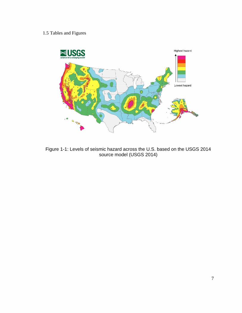
motions). A majority of the Pacific Northwest (PNW) is faced with a moderate to
high seismic hazard levels (Figure 1-1), with a sizeable portion of the hazard
stemming from the Cascadia Subduction Zone (CSZ). This means that for
practitioners in the PNW, the effects of inelasticity and long duration ground
motions are of particular concern. With the emergence of performance-based
earthquake engineering, the shortcomings in the current recommendations are
emphasized because of the increased emphasis that performance based
earthquake engineering places on estimates of deformation (Bozorgnia and
Bertero 2004). It is essential that the displacement demands computed from
simplified procedures, such as equivalent static analysis (ESA), are consistent
with the demands obtained from more refined analysis methods, such as
nonlinear dynamic analysis (NDA).

3
1.2 Literature review
Since the early 1990’s research regarding lateral spreading and soil foundation
structure interaction (SFSI) has seen a sharp uptick. As the field continues to
evolve, new papers and recommendations will accompany our increasing
knowledge of the subject. The discussion in this section only serves to introduce
some of the most relevant or seminal papers on the topic covered in this
research.
Early recommendations regarding the combination of inertial and kinematic loads
in piles were provided by Martin et al. (2002), who recommended that the two
load cases be considered independently. This recommendation was based on
the idea that the two loads are unlikely to peak simultaneously. Therefore, it was
believed that designers could simply analyze the two cases separately and
envelope the pile response; however, the authors of the study recognized the
fact that our understanding of the mechanisms involved in this particular SFSI
problem was limited. Furthermore, they acknowledged the notion that long
duration motions may increase the probability that these two forces could interact
constructively.
Chang et al. (2006), Tokimatsu et al. (2005) and Brandenberg et al. (2005)
showed that the interaction between inertial and kinematic loads could act in or
out of phase. Boulanger et al. (2007) showed that inertial demands from the
superstructure on elastic piles in the liquefied case (i.e. with lateral spreading)

4
ranged from about 30% to 50% of the inertial demands in nonliquefied
conditions, depending on the frequency content of the input motion. Ashford et al.
(2011) synthesized a decade’s worth of research on the topic and presented a
design recommendation for bridge pile foundations in the same combination of
inertial and kinematic loading recommended by Boulanger (2007) was adopted.
This design recommendation eventually served as the primary basis for the
development of the Caltrans (2012) 50% inertia recommendation. Khosravifar
(2011) explored the interaction between kinematic and inertial loads for inelastic
piles using nonlinear dynamic analysis (NDA) methods, including a rather
expansive parametric study. He found that the equivalent static analysis (ESA)
procedure resulted in more accurate estimates of pile head displacements
(relative to NDA analysis) when 100% of the inertial displacement demands are
combined with the kinematic loading.
The Oregon Department of Transportation Geotechnical Design Manual (2014)
currently defers to the Ashford et al. (2012) guideline of combining 50% of the
nonliquefied inertial load with 100% of the liquefied kinematic load. The
Washington State Department of Transportation (WSDOT 2015) differs from its
two neighboring west coast states regarding the combination of inertial and
kinematic loading. WSDOT currently recommends 25% of the nonliquefied
inertial force in combination with 100% of the liquefied kinematic force.
The discrepancy between current design guidelines is a proverbial “red flag” for
practitioners involved in the design of inelastic piles. The issue is exacerbated by

5
the fact that Oregon practitioners are faced with a seismogenic source capable of
generating long duration ground motions, a factor that was not considered in the
codified kinematic and inertial loading combination factors. There is a need to
investigate the effects of long-duration ground motions and pile inelasticity on the
adequacy of Caltrans’ simplified ESA procedure.
1.3 Research objective
The primary objective of this research is to develop a design guideline for the
inelastic behavior of piles due to liquefaction-induced lateral spreading and
superstructure inertia. The revised guideline will include the effects of pile
inelasticity and long duration ground motions by utilizing a site-specific ground
motion analysis framework that is in general accordance with the current state of
practice in Oregon.
1.4 Structure of thesis
One of the aims of this paper is to present the research findings in a manner that
is most useful to geotechnical practitioners in the region. As such, the structure of
this thesis attempts to mirror the workflow involved in a typical site specific
seismic hazard analysis. The organization of the thesis is as follows:
• Chapter 2 discusses the site-specific hazard analysis for two sites
selected in Oregon. This includes a discussion of the relevant
seismogenic sources, probabilistic seismic hazard analysis (PSHA),

6
deterministic seismic hazard analysis (DSHA), and target spectra
development.
• Chapter 3 includes discussion of the ground motion selection process for
each site, along with the ground motion scaling and matching processes
that were used to modify the original ground motion response spectra.
• Chapter 4 presents an overview of the finite element (FE) model used in
the study. The discussion includes various components of the NDA model
such as the soil elements, structural elements, and p-y springs.
Furthermore, an example dynamic response of the NDA model and the
relevant results is provided in this chapter.
• Chapter 5 presents an overview of the ESA model and the results of ESA
in accordance with Caltrans and ODOT. The results from the ESA are
compared to the those of the NDA The comparison between the methods
serves as the basis for the proposed revision to Caltrans’ guidance, which
is also presented in this chapter.
• Chapter 6 presents a discussion regarding the results of the study and
provides a summary of the key findings. In addition, limitations in the work
are identified and recommendations for future research are provided.
7
1.5 Tables and Figures
Figure 1-1: Levels of seismic hazard across the U.S. based on the USGS 2014 source model (USGS 2014)

8
2 SITE-SPECIFIC SEISMIC HAZARD ANALYSIS
2.1 Background
Oregon’s seismicity presents interesting challenges for local practitioners. Much
of Oregon’s more heavily populated western half faces some level of threat from
either shallow crustal Quaternary faults or the Cascadia Subduction Zone (CSZ).
Wong (1995) presented a strong case for Oregonians to increase their
awareness of the seismic hazard in this region, while alluding to the fact that
Oregon is sometimes overlooked in terms of its seismic hazard. The state
contains crustal faults capable of generating Mw=7.0 or greater earthquakes in
Portland and other areas in eastern Oregon, as well as the offshore CSZ that can
generate earthquakes up to Mw=9.2 (USGS 2008).
While a characteristic earthquake on the PFH would likely cause more severe
damage around the Portland-Metro region (Wong 1995), the mega earthquake
potential of the CSZ has managed to capture the attention of the public and state
officials alike. In 2013 the Oregon Seismic Safety Policy Advisory Committee
(OSSPAC) presented the Oregon Resilience Plan to the state legislature. The
OSSPAC is made up of 18 individuals from across the state that represent a
wide variety of interests regarding public policy related to earthquakes. Their
plan, the Oregon Resilience Plan, was the culmination of a two-year-long effort to

9
present recommendations regarding the state-wide impact of a large earthquake
and how best to mitigate and prepare for the dire consequences that would likely
follow. Their study estimated tens of billions of dollars in damage to property and
infrastructure alone (i.e. economic impacts were not included in the estimate) for
a potential CSZ earthquake. Figure 2-1 shows a map of damage potential that
was generated for a moment-magnitude 9.0 CSZ earthquake (OSSPAC 2013).
Nearly a quarter of the state, stretching from the Oregon coast as far east as
Portland, is expected to be moderately to heavily damaged. It is clear that the
seismic hazard in Oregon presents some unique considerations due to its
seismogenic setting and the tremendous social and economic costs associated
with a characteristic event for either of these two sources.
Under severe levels of ground shaking that have the potential to occur across the
state, liquefaction and lateral spreading will undoubtedly affect some portion of
our existing infrastructure. For these cases, AASHTO (2014) and ASCE 7-10
require site specific site response analysis, which will be referred to from here on
out as site-specific procedure (SSP). The goal of any SSP is to more accurately
estimate the propagation of ground motions up a soil column to some point of
interest, usually taken as the ground surface. An SSP with thoughtful input
parameters can provide the engineer with more confidence in the soil response
and subsequently, the demands on the structure.
This chapter begins by discussing the site selection process for the study and the
seismogenic setting of the chosen sites. The remainder of the chapter is devoted

10
to discussion of the PSHA (probabilistic seismic hazard analysis), DSHA
(deterministic seismic hazard analysis), development of the requisite target
spectra, and finally the governing spectra for design.
2.2 Site selection
While geotechnical practitioners are often constrained to analyzing sites that are
presented to them by clients or contractors, this study provided an opportunity
select the hypothetical project sites. Recognizing that the effect of strong motion
duration on the interaction of kinematic and inertial loading was of primary
importance, it was essential that the chosen sites provide response data across a
spectrum of potential earthquake durations.
The first site that was chosen was is in Oregon’s most heavily populated city,
Portland (U.S. Census 2010). Portland is also Oregon’s most seismically active
region (Wong 1995). Table 2-1 provides the latitude and longitude of the
hypothetical project site. The site is located just west of the Willamette River,
which is a north/south trending river and is the major tributary of the Columbia
River. Very generally speaking, the geologic conditions in this area can be
described as recent Quaternary sand, silt, and gravel deposits overlying older
Quaternary sedimentary and volcanic rock deposits, in turn overlying Tertiary
volcanic rock (Trimble 1963). The fact that the city is split by the Willamette River
and has numerous bridges linking its eastern and western halves, in combination

11
with the moderately-high seismicity in the area, means the findings of this study
may be directly applicable to existing, or future, structures located in Portland.
The second hypothetical site was chosen in Astoria, Oregon. Astoria is one of
Oregon’s most populous coastal cities, with nearly 10,000 inhabitants (U.S.
Census 2010). The city is located near the mouth of the Columbia River and is
home to two bridges that allow US Highway 101 to pass over Young’s Bay and
the Columbia River. The near-surface geologic deposits in the area are mostly
unconsolidated alluvial deposits or lower to middle-aged Miocene mudstone
deposits from the Astoria formation (Niem and Niem 1985). The site coordinates
are provided in Table 2-1.
2.3 Seismicity
2.3.1 Cascadia Subduction Zone
At approximately 700 miles long, the CSZ zone stretches along the Pacific Coast
from British Columbia to northern California. It occurs at a convergent boundary
between the North American plate and several smaller plates. More specifically,
off the coast of Oregon and Washington it is the Juan DeFuca plate that is
subducting beneath the North American plate at an average rate of 1.6-inches
per year (CREW 2013). This build-up and eventual release of strain energy will
cause the next great Cascadia earthquake.
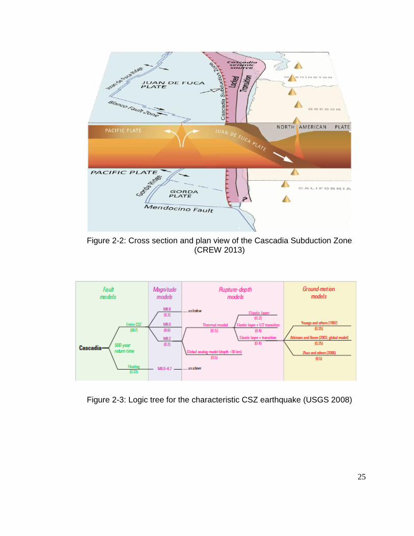
Figure 2-2 shows a combined plan and cross-sectional view of the boundary
between the plates in the CSZ. It is clear that a portion of the Juan De Fuca plate

12
has already descended beneath the overriding North American plate and
subsequently, the state of Oregon. Off the coast of the Pacific Ocean, though,
where the North American Plate and the Juan De Fuca come together, exists a
“locked zone.” The “locked zone” can be thought of as the region where the
colliding plates are stuck together, constantly accumulating strain (CREW 2013).
The distinction between the locked zone and the portion of the Juan De Fuca that
has already subducted beneath the North American plate is an important one
because it gives rise to very different potentials for ground motion intensity.
Investigators have categorized potential CSZ earthquakes by the depth at which
they are likely to occur. Shallow, or “interface,” earthquakes occur at a depth up
of 20 to 40 miles (depending on site location) below the surface of the earth,
which corresponds to a rupture within the locked portion of the CSZ. The
magnitude 9 scenario is usually attributed to this type of shallow rupture. On the
other hand, deeper and less intense earthquakes can occur in the portion of the
CSZ where the Juan De Fuca slab has already subducted; these types of
earthquakes are known as “intraslab” earthquakes, and they occur at depths
below the interface zone. Figure 2-3 provides the logic tree used to model a CSZ
rupture for the 2008 USGS source model.
2.3.2 Shallow crustal
Since ground motion intensity dissipates with increased distance between the
source and the receiver, smaller magnitude crustal earthquakes at shorter

13
source-to-site distances are capable of producing intense shaking in areas near
the rupture. The downtown Portland area is thought to contain three active faults:
the Oatfield Fault, the Eastbank Fault, and the Portland Hills Fault (PHF). Wong
et al. (2001) provide a thorough discussion regarding the characterization of the
PHF and to some extent, the Eastbank and Oatfield Faults. However, the East
Bank and Oatfield faults were not explicitly included in the 2008 or 2014 USGS
probabilistic seismic hazard studies; instead, these faults are considered as part
of the Portland Hills Fault zone.
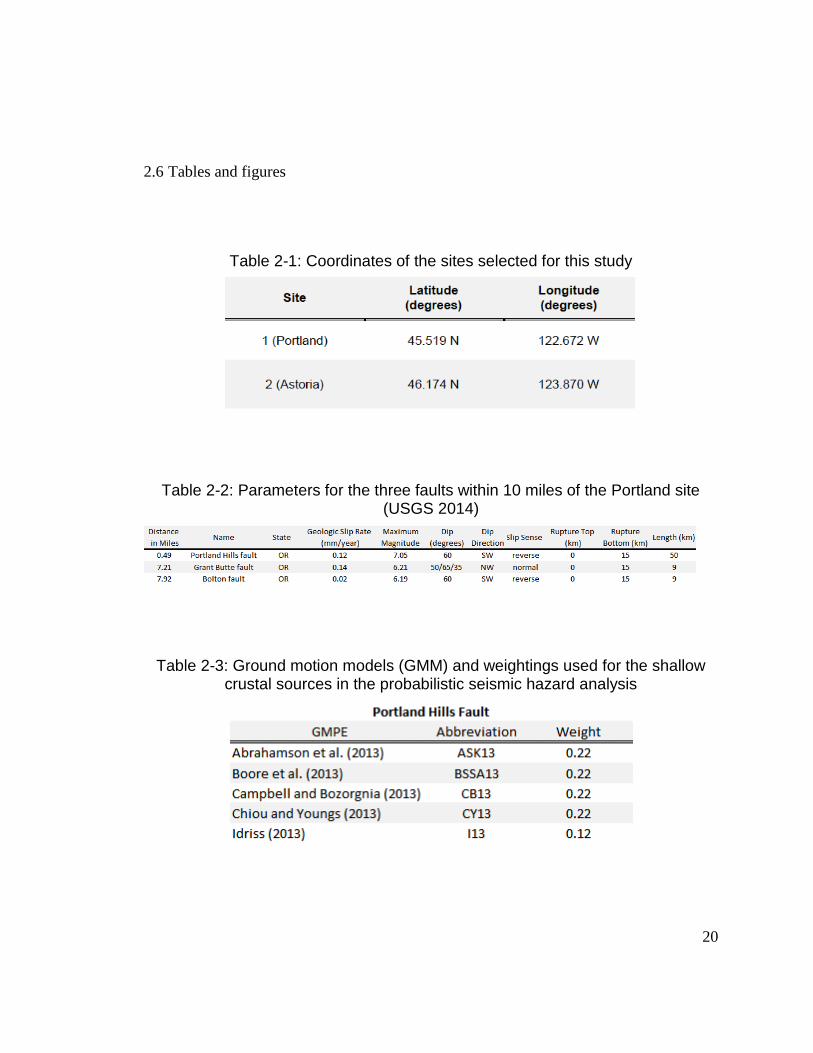
Based on the USGS Seismic Hazard Map Documentation (2008), there are three
active faults located within 10 miles of Portland. The three faults and their
respective parameters are shown in Table 2-2. Only the PHF was considered for
further analysis because it can produce the largest earthquake at the shortest
distance from the site.
2.4 PSHA and DSHA
The target design spectra were developed based on site-specific procedures
outlined in ASCE 7-10 (MCER) and AASHTO (975-year return period). These
procedures require performing probabilistic seismic hazard analysis (PSHA) and
deterministic seismic hazard analysis (DSHA) as described in the next sections.
The target spectra were developed for Site Class B/C (Vs = 760 m/s) and were
later used in site-response analysis described in Chapter 4.
14
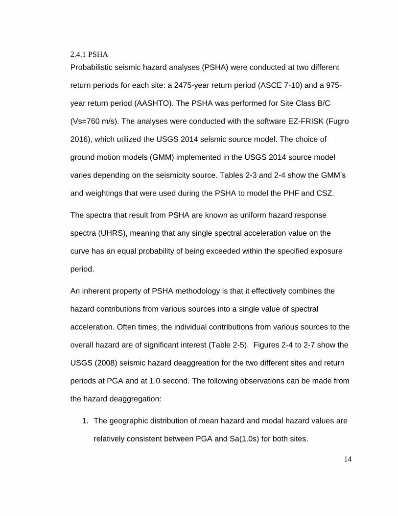
2.4.1 PSHA
Probabilistic seismic hazard analyses (PSHA) were conducted at two different
return periods for each site: a 2475-year return period (ASCE 7-10) and a 975-
year return period (AASHTO). The PSHA was performed for Site Class B/C
(Vs=760 m/s). The analyses were conducted with the software EZ-FRISK (Fugro
2016), which utilized the USGS 2014 seismic source model. The choice of
ground motion models (GMM) implemented in the USGS 2014 source model
varies depending on the seismicity source. Tables 2-3 and 2-4 show the GMM’s
and weightings that were used during the PSHA to model the PHF and CSZ.
The spectra that result from PSHA are known as uniform hazard response
spectra (UHRS), meaning that any single spectral acceleration value on the
curve has an equal probability of being exceeded within the specified exposure
period.
An inherent property of PSHA methodology is that it effectively combines the
hazard contributions from various sources into a single value of spectral
acceleration. Often times, the individual contributions from various sources to the
overall hazard are of significant interest (Table 2-5). Figures 2-4 to 2-7 show the
USGS (2008) seismic hazard deaggreation for the two different sites and return
periods at PGA and at 1.0 second. The following observations can be made from
the hazard deaggregation:
1. The geographic distribution of mean hazard and modal hazard values are
relatively consistent between PGA and Sa(1.0s) for both sites.

15
2. The hazard to the Portland site is predominantly coming from two distinct
regions.
3. A substantial portion of the hazard to the Astoria site can be attributed to
a single region.
In Astoria, the seismic hazard is dominated by the CSZ (corresponding to
earthquake magnitude Mw = ~9 at source-to-site distance of ~19 km), which is
represented by the large cluster of bars at short distance in the geographic
deaggregation. In this case, the mean hazard and the modal hazard are nearly
identical because they are essentially coming from a single source, with the only
differences stemming from the different fault rupture schemes that the USGS
considered for the CSZ.
For the Portland site, the hazard has a bi-modal distribution as shown by the two
large clusters of bars on the deaggregation figures (corresponding to Mw= 9 and
source-to-site distance~90 km for the CSZ and Mw=7 and source-to-site distance
of ~1 km).
2.4.2 DSHA
A deterministic seismic hazard analysis (DSHA) is an alternate method of
quantifying the seismic hazard at a site, wherein specific earthquake scenarios
are explicitly considered. The resulting envelope of spectral acceleration
ordinates, for the different scenarios, is usually adopted as the target response
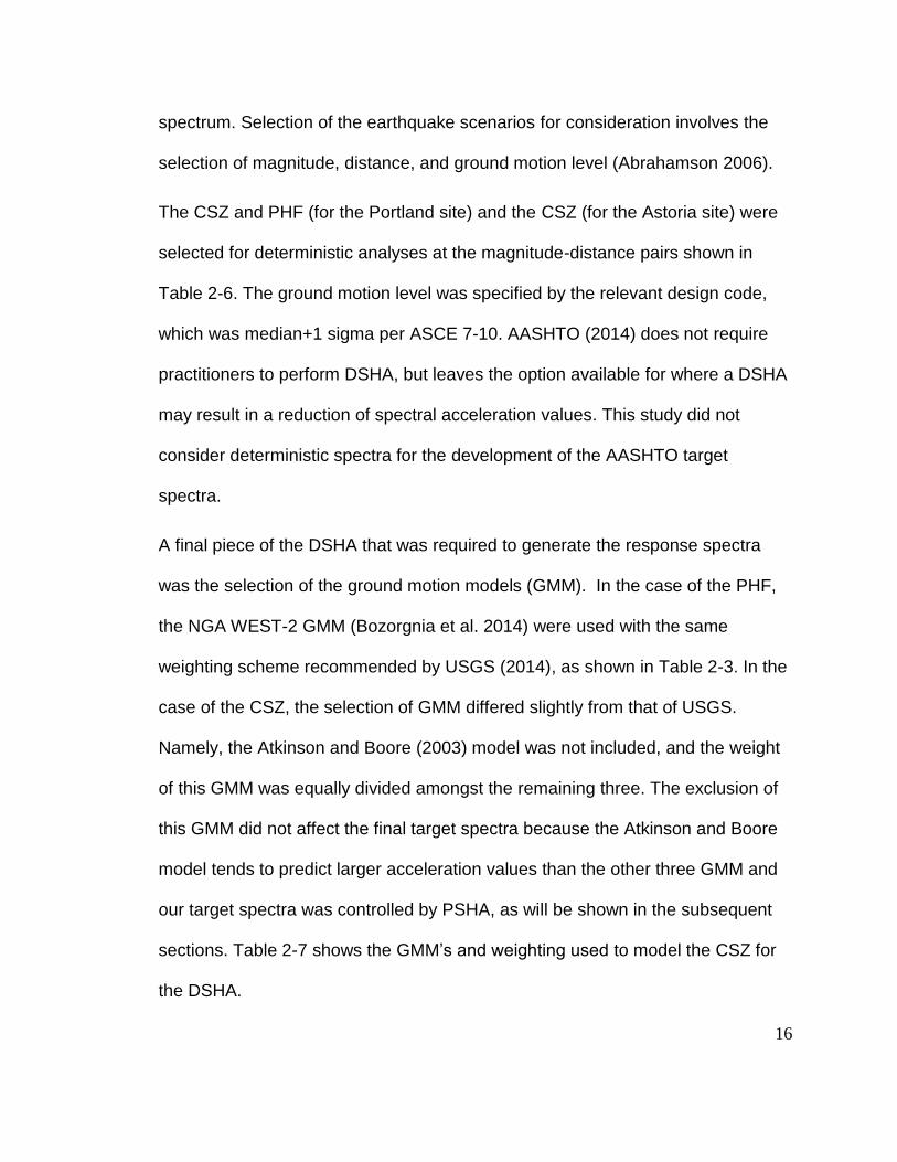
16
spectrum. Selection of the earthquake scenarios for consideration involves the
selection of magnitude, distance, and ground motion level (Abrahamson 2006).
The CSZ and PHF (for the Portland site) and the CSZ (for the Astoria site) were
selected for deterministic analyses at the magnitude-distance pairs shown in
Table 2-6. The ground motion level was specified by the relevant design code,
which was median+1 sigma per ASCE 7-10. AASHTO (2014) does not require
practitioners to perform DSHA, but leaves the option available for where a DSHA
may result in a reduction of spectral acceleration values. This study did not
consider deterministic spectra for the development of the AASHTO target
spectra.
A final piece of the DSHA that was required to generate the response spectra
was the selection of the ground motion models (GMM). In the case of the PHF,
the NGA WEST-2 GMM (Bozorgnia et al. 2014) were used with the same
weighting scheme recommended by USGS (2014), as shown in Table 2-3. In the
case of the CSZ, the selection of GMM differed slightly from that of USGS.
Namely, the Atkinson and Boore (2003) model was not included, and the weight
of this GMM was equally divided amongst the remaining three. The exclusion of
this GMM did not affect the final target spectra because the Atkinson and Boore
model tends to predict larger acceleration values than the other three GMM and
our target spectra was controlled by PSHA, as will be shown in the subsequent
sections. Table 2-7 shows the GMM’s and weighting used to model the CSZ for
the DSHA.

17
The resulting spectra and their weighted geometric means are shown in Figures
2-8 to 2-10. Figure 2-11 shows the weighted geometric mean spectra for the two
sources in Portland. For a 2475-year return period and the chosen weighting
scheme, the PHF controls the spectral response up to a period of approximately
3 seconds, at which point the CSZ controls.
2.5 Target spectra development
The spectra that were obtained from the PSHA and DSHA were adjusted in
accordance with ASCE 7-10 and AASHTO (2014) in order to generate the final
target spectra for each scenario. This means that the 2475-year return period
UHRS and the median+1 sigma DSHA spectra were adjusted and checked
against minimum values in accordance with ASCE 7-10 guidelines, while the
975-year return period UHRS were modified and compared against AASHTO
(2014) minimum values.
The Risk-Targeted Maximum Considered (MCER) response spectra were
developed based on ASCE 7-10 in the general sequence described below:
1. The UHRS spectral acceleration values were scaled by the USGS risk
coefficients to yield the risk targeted response spectra for a 1% probability
of collapse within a 50-year period. Table 2-8 shows the risk coefficients
that were extracted from the USGS seismic design application
(https://earthquake.usgs.gov/designmaps/us/application.php) and used in
the analysis.

18
a. The risk-targeted acceleration values were scaled by the maximum
rotated component factors presented in ASCE 7-10 Supplement 1
(2013) to account for the fact that the GMM’s report the geometric
mean of the horizontal response. Table 2-8 shows the maximum
rotation factors that were used.
2. The DSHA spectral values were scaled by the same maximum rotation
factors
a. The maximum rotated deterministic spectra were checked against
the deterministic limit per ASCE 7-10 and the larger of the spectral
acceleration values at any given period was used
3. The resulting maximum rotated deterministic spectrum was compared
against the maximum rotated risk targeted probabilistic spectrum and the
lesser of the spectral acceleration values at any given period was selected
(Figures 2-12 and 2-13).
The development of the AASHTO target spectra was less complex, as the code
does not require any a risk or directionality adjustments. In this case, each of the
975-year UHRS was simply checked against its respective code-based minimum
spectrum. The code-based minimum spectrum was taken as 2/3 of the spectrum
generated by the USGS Seismic Design Tool (2008) (without risk or rotation
factors), adjusted for site effects. The relevant spectra from this process are
shown in Figures 2-14 and 2-15.

19
2.5.1 Final target spectra
The final result was four target spectra, an MCER and an AASHTO spectrum for
each site. Figure 2-16 shows all four spectra on a single plot and Table 2-9
provides the spectral ordinates in tabulated form. The MCER spectra for Portland
and Astoria were governed by PSHA across all periods. In fact, the deterministic
spectral acceleration values were substantially larger across the entire period
range of interest. In the case of the AASHTO target spectra, the probabilistic
spectra controlled across all but very long periods (T <6 seconds), beyond which
the 2/3 code based spectra controlled.
20
2.6 Tables and figures
Table 2-1: Coordinates of the sites selected for this study
Table 2-2: Parameters for the three faults within 10 miles of the Portland site (USGS 2014)
Table 2-3: Ground motion models (GMM) and weightings used for the shallow crustal sources in the probabilistic seismic hazard analysis

21
Table 2-4: Ground Motion Models (GMM) and weightings used to model the Cascadia Subduction Zone in the probabilistic seismic hazard analysis
Table 2-5: Summary of hazard deaggregation results
Hazard Contribution (rounded to nearest percent) *
PSHA
Scenario
Structural
Period
CSZ
(interface)**
CSZ
(intraslab)** PHF
All Other
Sources
Portland
2475-
year
PGA 32% 19% 21% 28%
T=1 sec 61% 13% 16% 10%
Portland
975-year
PGA 33% 22% 11% 34%
T=1 sec 57% 18% 9% 16%
Astoria
2475-
year
PGA 98% 2% 0% 0%
T=1 sec 98% 0% 0% 2%
PGA 91% 9% 0% 0%

22
Astoria
975-year T=1 sec 95% 5% 0% 0%
*based on USGS 2008 deaggregation (v3.3.1), rounded to nearest whole percent
**summation of contribution from different rupture/faulting scenarios
Table 2-6: Magnitude and distance pairs used for deterministic seismic hazard analyses
Table 2-7: GMM's and weighting used to model the Cascadia Subduction Zone in the deterministic seismic hazard analysis

23
Table 2-8: Risk and maximum rotation coefficients, per ASCE 7-10, for the two sites
Max. Rot. Factor

24
Table 2-9: Target spectra per ASCE 7-10 and AASHTO LRFD (2014)
Figure 2-1: Estimated impact zones within Oregon for a characteristic CSZ event -damage will be extreme in the Tsunami zone, heavy in the Coastal zone,
moderate in the Valley zone, and light in the Eastern zone (OSSPAC 2013)
25
Figure 2-2: Cross section and plan view of the Cascadia Subduction Zone (CREW 2013)
Figure 2-3: Logic tree for the characteristic CSZ earthquake (USGS 2008)

26
Figure 2-4: Portland seismic hazard deaggregation for the 2475-year return period at PGA (top) and T=1.0 second (bottom) (USGS 2008)

27
Figure 2-5: Portland seismic hazard deaggregation for the 975-year return period at PGA (top) and T=1.0 second (bottom) (USGS 2008

28
Figure 2-6: Astoria seismic hazard deaggregation for the 2475-year return period at PGA (top) and T=1.0 second (bottom) (USGS 2008)

29
Figure 2-7: Astoria seismic hazard deaggregation for the 975-year return period at PGA (top) and T=1.0 second (bottom) (USGS 2008)

30
Figure 2-8: Median + 1 sigma deterministic spectra for the Cascadia Subduction Zone at the Portland site

31
Figure 2-9: Median + 1 sigma deterministic spectra for the Portland Hills Fault at the Portland site

32
Figure 2-10: Median + 1 sigma deterministic spectra for the Cascadia Subduction Zone at the Astoria site

33
Figure 2-11: Comparison of the deterministic spectra for the two sources at the Portland site

34
Figure 2-12: Development of the target MCER spectrum, per ASCE 7-10, for the Portland site

35
Figure 2-13: Development of the target MCER spectrum, per ASCE 7-10, for the Astoria site

36
Figure 2-14: Development of the AASHTO LRFD (2014) target spectrum for the Portland site
0.0
0.1
0.2
0.3
0.4
0.5
0.6
0.7
0.01 0.1 1 10
Sa (
g)
Period (s)
AASHTO
2/3 AASHTO
PSHA 975-yr

37
Figure 2-15: Development of the AASHTO LRFD (2014) target spectrum for the Astoria site
0.0
0.2
0.4
0.6
0.8
1.0
1.2
0.01 0.1 1 10
Sa (
g)
Period (s)
AASHTO
2/3 AASHTO
PSHA 975-yr

38
Figure 2-16: Comparison of the target spectra for Portland and Astoria sites

39
3 GROUND MOTION SELECTION AND MODIFICATION
3.1 Ground motion selection
Seven ground motion records were selected for each site as eventual input to the
nonlinear dynamic analyses (NDA). The selection of the ground motion records
was based on a multitude of factors, including:
• earthquake magnitude,
• source to site distance,
• site conditions (namely the shear wave velocity in the upper 30-meters -
Vs30),
• and rupture mechanism (e.g. subduction, reverse, normal, etc.).
The relative proportion of ground motion records chosen to represent each
seismic source was based on the USGS deaggregation results discussed in
Chapter 2.
As previously mentioned, both sites experience significant hazard contribution
from the Cascadia Subduction Zone (CSZ). The characteristic earthquake
associated with the CSZ (magnitude 9) would be a historically intense ground
motion, meaning that the database of available recordings from similar events is

40
few and far between. This presents a challenge for practitioners in need of
multiple large magnitude ground motion records. The relatively recent Tohoku
(magnitude 9) and Maule (magnitude 8.8) earthquakes have alleviated the issue
to some extent, but the result is that many ground motion suites contain multiple
records from these two events and this study is no exception. The use of multiple
recordings from the same event is quite common in the Pacific Northwest, and is
essentially unavoidable due to the lack of large magnitude events with recorded
time histories.
Figures 3-1 to 3-6 show the acceleration, velocity, and displacement time
histories of the ground motions that were selected for Portland and Astoria,
respectively. The fourteen selected ground motions were eventually modified for
compatibility with their respective target spectra. This was accomplished for both
sites using the common linear scaling method. In the case of the Portland site, an
additional spectral matching routine was performed in addition to the scaling.
The following sections provide information regarding the seed ground motions
and the modification processes used to generate the target spectrum compatible
time histories for NDA input.
3.1.1 Portland
The seven motions that were selected for Portland are shown in Table 3-1, along
with their key characteristics. The ground motion records were selected based on
the deaggregated hazard data (Table 2-5) and the aforementioned factors, such

41
as site conditions, rupture mechanics, etc. They include four shallow crustal
records, two interface subduction records, and one intraplate subduction record.
The hazard contribution for the 975-year return period followed a similar
breakdown, which allowed for the same ground motion suite to be used for both
return periods.
The selection of ground motion records used to represent local crustal events
was performed using the PEER NGA-West2 online tool
(http://ngawest2.berkeley.edu/). The selection of earthquake records was further
refined to account for the probability of pulse motions due to the proximity of the
PHF. The method of Hayden et al. (2014) was used to estimate the probability of
pulse motions based on the spectral acceleration at a period of 1-second and the
epsilon value of the ground motion. The result was that two of the four crustal
motions include a velocity pulse, as classified by PEER (2013). The 1989 Loma
Prieta earthquake record, taken from the Lexington Dam station, was recorded
on the dam abutment. The record was assumed to be representative of a free
field recording based on the work of Makdisi et al. (1994).
3.1.2 Astoria
In the case of the Astoria site, the seismic hazard was unsurprisingly dominated
by the CSZ megaquake. A summation of various CSZ rupture scenarios
accounts for approximately 98% of the hazard for a 2475-year return period at
PGA (Table 2-5). The difference in magnitude and distance for the two scenarios

42
is due to the uncertainty involved in modelling the fault rupture mechanisms.
Table 3-2 shows the seven selected ground motions that were chosen based on
the deaggregation. Two ground motion records from each, Tohoku and Maule,
were used due to the previously discussed lack of similar strong motion
recordings.
3.2 Ground motion scaling
Linear ground motion scaling is a common method of ground modification in
which an acceleration time history is multiplied by a constant factor in order to
improve the spectral fit across the structure’s period range of interest. The period
range of interest is usually taken as 0.2*T to 1.5*T, where T is the fundamental
period of the structure, to account for both higher mode response and period
lengthening due to inelasticity (NIST 2011). For the single soil-pile system
considered in this analysis the fundamental period of the structure can be
approximated as 1.4 seconds, as will be shown in the subsequent chapters.
Typically, peaks and valleys in the response spectrum of an individual ground
motion make it difficult to adequately scale the record using a constant factor. Bi-
modal hazard distributions stemming from different fault mechanisms can further
complicate the scaling process because of the different characteristics of the
expected motions. For instance, the target spectrum that was derived from the
probabilistic hazard analysis at the Portland site is dominated by the PHF at short
to intermediate periods and the CSZ at long periods. This means that a single

43
ground motion event is unlikely to produce a response spectrum with the same
shape as the target. For this reason, linear scaling of either a subduction or
crustal event to match the entire target spectrum can be challenging. It is
important to remember that the goal of the scaling process is to obtain an
average response across the entire suite of motions that is in line with the target
spectrum.
The scale factors used for the ground motions in Portland and Astoria are shown
in Tables 3-3 and 3-4, respectively. These scale factors were chosen based on
the resulting fit to the target spectrum across the period range of interest and at
PGA. While most of the scale factors fall within reasonable limits, it should be
noted that the Talagante recording from the 2015 Illapel, Chile earthquake
required scale factors greater than 6 to achieve a reasonable fit with the target
spectra. Although there is no strict limit regarding the maximum magnitude of
scale factors, it is worth recognizing that in this case the scale factors were
outside of the preferred range. The resulting scaled spectra are shown, plotted
against their respective target spectra in Figures 3-7 to 3-10.
3.3 Ground motion matching
Spectral matching is a ground motion modification procedure in which the
frequency content of a seed ground motion is adjusted in order to improve the
agreement between the spectral response and target spectrum. While the
matching procedure often results in a higher degree of compatibility across the

44
entire target spectrum (relative to linear scaling), it also reduces the variability of
the structural response. For the purpose of this study, the reduction of variability
was an advantageous consequence because it isolated the differences in
structural response solely due to the effects of strong motion duration.
Spectral matching was performed using RspMatch (Al Atik and Abrahamson
2010). Initially, the Portland set of ground motions were matched to the AASHTO
target spectrum. The matched set of motions was then linearly scaled to the
MCER level using a constant factor of 1.7, which corresponds to the ratio of PGA
between the MCER and AASHTO spectra. A reasonably good fit to the MCER
target was obtained due to the similarity in shape between the two target spectra.
Figures 3-11 to 3-17 show comparisons between the 7 original time histories and
their spectrally matched counterparts. Figures 18 and 19 show the resulting
matched spectra and their respective targets. Generally, the matched spectra are
in good agreement with target spectra and the velocity time histories generally
retained their key characteristics

45
3.4 Tables and Figures
Table 3-1: Ground motions selected for the Portland site and their key characteristics
Event
Tohoku, Japan
March 3, 2011
Maule, Chile
February 27, 2010
Offshore, El Salv.
January 13, 2001
Tabas, Iran September
16, 1978
Nahanni, Canada
December 23, 1985
Cape Mendocino, CA April 25,
1992
Loma Prieta,
CA October 17, 1989
Station Tajiri
(MYGH06)
Cerro Santa Lucia (STL)
Acajutla Cepa (CA)
Tabas (TAB)
Site 1 Cape
Mendocino (CPM)
Los Gatos-
Lex. Dam (LEX)
Component NS 360 90 T1 280 00 90
Magnitude 9.0 8.8 7.7 7.35 6.76 7.01 6.93
Rupture Distance
(km) 63.8 64.9 151.8* 2.05 9.6 6.96 5.02
Vs30 (m/s)
593 1411 Intermediate
Intrusive Rock
767 605 568 1070
Rupture Mechanism
Subduction (Interface)
Subduction (Interface)
Subduction (Intraslab)
Crustal (Reverse)
Crustal (Reverse)
Crustal (Reverse)
Crustal (Reverse Oblique)
D5-95 (sec) 85.5 40.7 27.2 16.5 7.5 9.7 4.3
PGA(g) 0.27 0.24 0.10 0.87 1.25 1.51 0.41
Pulse No No No Yes No No Yes

46
Table 3-2: Ground motions selected for the Astoria site and their key characteristics
Event
Tohoku, Japan
March 3, 2011
Tohoku, Japan
March 3, 2011
Maule, Chile February 27,
2010
Maule, Chile
February 27, 2010
Mexico City, Mexico
September 19,1985
Illapel, Chile
September 16, 2015
Arequipa, Peru
June 23, 2001
Station Tajiri
(MYGH06) Matsudo
(CHB002)
Cien Agronomicas
(ANTU)
Cerro Santa Lucia (STL)
La Union (UNIO)
Talagante (TAL)
Moquegua (MOQ)
Component NS NS NS 360 N00W 90 NS
Magnitude 9.0 9.0 8.8 8.8 8.0 8.3 8.4
Rupture Distance
(km) 63.8 356.0* 64.6 64.9 83.9* 140.9 76.7
Vs30 (m/s)
593 325** 621 1411 Meta-
Andesite Breccia
1127 573
Rupture Mechanism
Subduction (Interface)
Subduction (Interface)
Subduction (Interface)
Subduction (Interface)
Subduction (Interface)
Subduction (Interface)
Subduction (Interface)
D5-95 (sec) 85.5 47.1 38.5 40.7 24.2 76.4 36.0
PGA(g) 0.27 0.29 0.23 0.24 0.17 0.065 0.22

47
Table 3-3: Scale factors for the Portland ground motions
Table 3-4: Scale factors for the Astoria ground motions
Event
Tohoku, Japan
March 3, 2011
Maule, Chile
February 27, 2010
Offshore, El Salv.
January 13, 2001
Tabas, Iran September
16, 1978
Nahanni, Canada
December 23, 1985
Cape Mendocino, CA April 25,
1992
Loma Prieta,
CA October 17, 1989
MCEr Scale Factor
1.38 1.85 3.61 0.51 0.42 0.32 1.11
AASHTO Scale Factor
0.86 1.16 2.26 0.32 0.26 0.2 0.69
Event
Tohoku, Japan
March 3, 2011
Tohoku, Japan
March 3, 2011
Maule, Chile
February 27, 2010
Maule, Chile
February 27, 2010
Mexico City, Mexico
September 19,1985
Illapel, Chile
September 16, 2015
Arequipa, Peru
June 23, 2001
MCEr Scale Factor
2.35 3.00 2.75 3.00 4.50 10.20 3.10
AASHTO Scale Factor
1.40 1.60 1.80 1.80 2.75 6.50 1.90

48
Figure 3-1: Unscaled acceleration time histories of the 7 ground motions selected for Portland

49
Figure 3-2: Unscaled acceleration time histories of the 7 ground motions selected for Astoria

50
Figure 3-3: Unscaled velocity time histories of the 7 ground motions selected for Portland

51
Figure 3-4: Unscaled velocity time histories of the 7 ground motions selected for Astoria

52
Figure 3-5: Unscaled displacement time histories of the 7 ground motions selected for Portland

53
Figure 3-6: Unscaled displacement time histories of the 7 ground motions selected for Astoria

54
Figure 3-7: Individual ground motion spectra scaled to the MCER target spectrum at the Portland site

55
Figure 3-8: Individual ground motion spectra scaled to the MCER target spectrum at the Astoria site

56
Figure 3-9: Individual ground motion spectra scaled to the AASHTO target spectrum at the Portland site

57
Figure 3-10: Individual ground motion spectra scaled to the AASHTO target spectrum at the Astoria site

58
Figure 3-11: Comparison of original and matched motions for the 1978 Tabas earthquake at the Tabas station (component T1) at the Portland-AASHTO level

59
Figure 3-12: Comparison of original and matched motions for the 2010 Maule earthquake at the Cerro Santa Lucia station (component 360) at the Portland
AASHTO level

60
Figure 3-13: Comparison of original and matched motions for the 1985 Nahanni earthquake at the Site 1 station (component 280) at the Portland AASHTO level

61
Figure 3-14: Comparison of original and matched motions for the 2011 Tohoku earthquake at the Tajiri station (component NS) at the Portland AASHTO level

62
Figure 3-15: Comparison of original and matched motions for the 1989Loma Prieta earthquake at the Lexington Dam station (comp 90) at the Portland
AASHTO level

63
Figure 3-16: Comparison of original and matched motions for the 1992 Cape Mendocino earthquake at the Cape Mendocino station (component 00) at the
Portland AASHTO level

64
Figure 3-17: Comparison of original and matched motions for the 2001 El Salvador earthquake at the Acajutla Cepa station (component 90) at the Portland
AASHTO level

65
Figure 3-18: Individual ground motion spectra matched to the AASHTO target spectrum for the Portland site

66
Figure 3-19: Individual ground motion spectra, originally matched to the AASHTO target at the Portland site, scaled by a factor of 1.7 to the MCEr level

67
4 NONLINEAR DYNAMIC ANALYSIS (NDA)
4.1 Background
This chapter focuses on providing a broad overview of the finite element (FE)
model used to perform the nonlinear dynamic analyses (NDA), the cases that
were considered in our analyses, and a summary of the NDA output. The
numerical model employed in this study was largely based on the model
developed by Khosravifar et al. (2014), with a few minor modifications. While
some discussion of the model details and calibration is presented herein, a more
detailed explanation regarding the technical merits of the model is provided by
Khosravifar et al. (2014).
4.2 Finite Element Model
A two-dimensional (2-D) finite element (FE) model was created in the OpenSees
framework. (Mazzoni et al. 2009).
The model consists of three main parts (Figure 4-1):
i. a 2-D soil column representing the far-field soil behavior,
ii. a reinforced concrete (RC) pile shaft, and

68
iii. interface elements (i.e. soil springs) that connect the RC pile and soil
column.
The advantages of modelling in 2-D versus 3-D include faster computational
times and simplified pre-and post-processing of results. The 3-D effect of soil
flowing around the pile is approximated in the 2-D model through the use of the
soil springs (p-y curves). These springs allow for large relative displacements
between the soil and the pile. For this reason, the 2-D model is expected to
provide a reasonable approximation of the 3-D behavior of laterally spreading soil
around the pile. Finally, the numerical modelling approach used in this study has
been shown to capture pore-water pressure build up, liquefaction triggering, post-
liquefaction accumulation of shear strains in the liquefied soil, first order
interaction between piles and liquefied soil, and timing/phasing of critical load
combinations reasonably well (Khosravifar et al. 2014).
The dynamic analyses (NDA) were performed for two conditions: (1) liquefied
sloped-ground condition, and (2) nonliquefied level-ground condition where pore-
water pressure generation was precluded. In the liquefied sloped-ground
condition, a static shear stress was applied to the soil model to simulate 10%
ground slope (α = 0.1). The following sections provide additional discussion
regarding individual components of the model, as well as a representative
dynamic response from FE model, and a summary of the NDA results.

69
4.2.1 Soil elements
The soil profile consists of a 5-meter thick clay crust (Su=40 kPa), over a 3-meter
thick loose sand layer ((N1)60=5), over a 12-meter thick dense sand layer
((N1)60=35). The soil was modeled using the Pressure-Dependent-Multi-Yield
(PDMY02) constitutive model for sand and the Pressure-Independent-Multi-Yield
(PIMY) for clay, in conjunction with the 9-4-Quad-UP elements (Yang et al.
2003). Figure 4-2 presents a generic depiction of the PDMY02 model behavior.
The 9-4-Quad-UP elements have 9 nodes with translational degrees-of-freedom
(DOF) and 4 pore-water pressure DOF. The soil elements were discretized into
heights of 0.5m. The soil column was assigned a large thickness (500-meters) to
preclude the effects of soil-pile reactions on the site response, thus capturing the
free-field soil behavior (Khosravifar et al. 2014).
The primary focus of the calibration process was to capture liquefaction triggering
and post-liquefaction accumulation of shear strains based on empirical or
mechanics-based correlations by Idriss and Boulanger (2008). Figures 4-3 and 4-
4 show the shear modulus, damping ratio reduction curves, and a simulated
cyclic direct simple shear test on the loose ((N1)60=5) sand. The PIMY model,
used for the clay layer, was calibrated based on the shear modulus and damping
ratio curves of Vucetic and Dobry (1991) for a clay with a plasticity index of 35.
Table 4-1 shows the parameters that were used to model each soil layer. In the
nonliquefaction cases, pore-water pressure generation in the PDMY02 model
was suppressed by adjusting contraction and dilation parameters so that shear

70
modulus and equivalent damping ratio behavior was unaffected (Khosravifar et
al. 2014).
4.2.2 Structural elements
The RC pile was 2-meters in diameter with 20-meter embedment and 5-meter
height above the ground. Pile element lengths were set at 0.5-meters. The pile
head to superstructure connection was free to rotate. The RC shaft was modeled
using fiber sections and nonlinear-beam-column elements with nonlinear stress-
strain behavior for reinforcing steel, confined concrete, and unconfined concrete
(Figure 4-5). This model is capable of capturing the nonlinear behavior of RC
piles and the formation of a plastic hinge at any depth. Figure 4-6 shows the
moment-curvature response of the RC shaft.
The concrete compressive strength (f’c) was equal to 44.8-MPa. The
superstructure dead load was modeled as a 7-MN lumped mass, corresponding
to an axial load ratio (f’c*Ag) of approximately 5%. The longitudinal steel ratio of
the RC column was 2%. The steel bars were modeled with a yield strength of
475-MPa, an elastic modulus of 200-GPa, and a strain hardening ratio of 3%.
4.2.3 Interface elements
The soil-pile interface was simulated using p-y, t-z, and q-z soil springs to model
lateral, side-friction, and end-bearing interface behavior, respectively. The spring
spacing was set at 0.5-meters. This value was refined enough so that pile
response was unaffected (Khosravifar et al. 2014). The soil-springs used to

71
model the clay were based on the Matlock (1970) p-y curves (Figure 4-7), while
the soil-spring parameters for the sand layers were selected based on guidance
from API (2000).
A special type of py and tz springs were used in the liquefied layer (implemented
as PyLiq and TzLiq in OpenSees) where the strength and stiffness of the springs
change in proportion to the excess-pore-water pressure ratio in the adjacent soil
element (Figure 4-8). These models have proven to be effective in capturing the
first-order effects of liquefaction during dynamic analyses (Brandenberg et al.
2013). A transition zone of 1 pile diameter in length was implemented for the soil-
springs above the dense sand layer and below the clay layer, to model the
weakening effect that the liquefied layer exerts on the overlying and underlying
nonliquefied layers (Yang and Yeremic 2002)
4.2.4 Ground motion
The input ground motions consisted of the 14 records that were selected and
modified as described in Chapter 3 (total of 42 individual cases). The ground
motions were applied as a shear stress at the base of the soil column, following
the compliant base procedure described by Mejia and Dawson (2006). The
dashpot coefficient was based on the mass density and shear wave velocity (760
m/s) of the bed rock half-space.

72
4.2.5 Solution Scheme
The FE solution scheme used the KrylovNewton solution algorithm and the β-
Newmark transient integrator with the constant acceleration scheme. Rayleigh.
damping of 0.5% at frequencies of 0.3 to 5 Hz was used for the soil column and
2% at the same frequencies for the RC shaft. The Rayleigh damping in soil was
used to account for small-strain damping and to reduce numerical “noise.”
Viscous radiation dashpots of p-y springs were assigned damping coefficients of
4ρDVs. The Vs value used to calculate the damping coefficient was computed as
10% of the pre-earthquake value to account for strain softening of the soil column
under earthquake loading.
4.2.6 Representative Dynamic Response
An example set of representative NDA results for one ground motion are
provided in Figure 4-9. The input motion used in the example is the 2010 Maule
earthquake (STL station) scaled to the AASHTO design spectrum developed for
the Portland site (PGA = 0.27 g). This is a subduction earthquake with a
significant duration, D5-95, of 40.7 seconds. The time of maximum pile head
displacement (0.17-meter downslope) is marked by a vertical dashed line in
Figure 4-9. At the time of maximum pile head displacement, the superstructure
inertia is 75% of its maximum and the lateral spreading force (crust load) is 70%
of its maximum. Note that at this time, liquefaction has already triggered
(ru=100%) and the lateral spreading load has almost fully mobilized. The relative

73
displacement between soil and pile is 0.35 meters; 0.4 meters of relative
displacement is required to fully mobilize the passive force in the clay crust.
4.3 Results
The relevant NDA results are presented in the following sections as it pertains to
either the site response portion of the analysis or the structural response of the
pile. It is important to remember that FE model was capable of modelling both
aspects of interest (the geotechnical and structural response) simultaneously and
the results are merely presented in this manner for clarity.
4.3.1 Site response analysis
The site response results for nonliquefied level ground and liquefied sloped
ground (α=0.1) for each site, and for both ground motion levels, is presented in
Figures 4-10 to 4-15 by plotting the spectral amplification ratios (SAR). The SAR
in this case is computed as the spectral acceleration recorded at the ground
surface of the soil column relative to the spectral acceleration of the bedrock
input motion (outcrop). In general, the site response results showed:
• deamplification at short structural periods in the nonliquefied case due to
the large ground motion intensity and nonlinear soil behavior,
• pronounced deamplification at short and intermediate structural periods in
the liquefied case due to liquefaction induced soil softening, and

74
• for any given site and hazard level, the maximum SAR was controlled by
the nonliquefied case up to a structural epriod of about 2 seconds, at
which point the liquefied case usually began to control the SAR envelope.
Lateral soil displacements were also of particular interest because of their effect
on the magnitude of passive pressure exerted on the RC shaft. The ground
surface displacement values were computed relative to the displacements at the
base of the soil column and were residual values (i.e. end of ground motion). The
displacement profiles in all of the liquefied cases followed the same general
pattern. The displacement was negligible through the dense sand layer and then
linearly increased through the liquefied layer to its maximum value where it
remained at a maximum through the clay crust. In the nonliquefied case,
maximum recorded soil displacements were negligible and the displacement
profiles varied in an unpredictable manner. As an example, Figure 4-16 shows a
representative set of soil displacement profiles fort the Portland set of ground
motions matched to the AASHTO target spectrum.
Note that approximately 0.4-meters of relative soil-pile displacement was
required to mobilize full passive pressure of the clay crust. Of the 42 different
cases that were analyzed under liquefied conditions, only 5 cases did not result
in enough relative ground surface displacement to mobilize the full passive
pressure; all 5 cases involved crustal motions at the Portland site. Figures 4-17
and 4-18 provide a comparison of the relative ground surface displacements for
all of the ground motion scenarios.

75
4.3.2 Structural response
Figures 4-19 and 4-20 show the maximum relative superstructure displacements
that occurred during each ground motion scenario. The displacements were
computed as the maximum pile head displacement at any time during the ground
motion relative to the base of soil column. As expected, the superstructure
displacements increase, for any given ground motion, when (1) the ground
motion intensity is greater (i.e. MCER level versus AASHTO) and (2) the effects
of liquefaction are included.
Figure 4-21 shows aggregated NDA results from all 42 input motions. The figure
compares the maximum pile head displacements between liquefied sloped-
ground conditions (combined inertial and kinematic demands) and nonliquefied
level-ground conditions (inertia only). The fact that all pile demands are larger in
the liquefied condition compared to the nonliquefied condition indicates that
demands cannot be enveloped by merely accounting for the effects of inertia only
or lateral spreading only (i.e. treating them separately). This finding is contrary to
the recommendations of MCEER/ATC (2003) that suggests designing piles for
the envelope of inertia and kinematics separately. Furthermore, these findings
are aligned with the results of other recent studies such as Tokimatsu et al.
(2005), Boulanger et al. (2007), Caltrans (2012), and Khosravifar et al. (2014).
The spectral response of the superstructure was also recorded during the NDA.
Figure 4-22 shows the nonliquefied SAR curves for the Portland site at the MCER
and AASHTO levels. The structural period of the system can be approximated

76
from these curves as 1.4-seconds in the nonliquefied condition. This value
compared favorably with the structural period obtained from the pushover curve,
as described in the subsequent chapter.

77
4.4 Tables and Figures
Table 4-1: Soil parameters used in the FE model (Khosravifar et al. 2014)

78
Figure 4-1: Depiction of the FE model
Figure 4-2: Pressure dependent multi yield surface model (Elgamal et al. 2001)

79
Figure 4-3: G/Gmax and equivalent damping ratios for undrained loading of sand with (N1)60=5
Figure 4-4: Undrained cyclic direct simple shear (DSS) simulation for sand with (N1)60=5

80
Figure 4-5: Cross section of the fiber section used to model the pile shaft
Figure 4-6: Moment-curvature behavior of the pile shaft
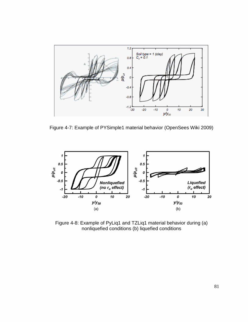
81
Figure 4-7: Example of PYSimple1 material behavior (OpenSees Wiki 2009)
Figure 4-8: Example of PyLiq1 and TZLiq1 material behavior during (a) nonliquefied conditions (b) liquefied conditions

82
Figure 4-9: Representative nonlinear dynamic analysis (NDA) results for the 2010 Maule EQ (Station STL) scaled by a factor of 1.16 for the AASHTO design
spectrum developed for the Portland site

83
Figure 4-10: Spectral amplification ratios (SAR) for the nonliquefied, level ground case (top) and liquefied case with α=0.1 (bottom) at the Portland site (ground
motions scaled to the MCEr target spectrum)

84
Figure 4-11: Spectral amplification ratios (SAR) for the nonliquefied level ground case (top) and liquefied case with α=0.1 (bottom) at the Portland site (ground
motions scaled to the AASHTO target spectrum)

85
Figure 4-12: Spectral amplification ratios (SAR) for the nonliquefied, level ground case (top) and liquefied case with α=0.1 (bottom) at the Portland site (ground
motions matched to the MCEr target spectrum)

86
Figure 4-13:Spectral amplification ratios (SAR) for the nonliquefied, level ground case (top) and liquefied case with α=0.1 (bottom) at the Portland site (ground
motions matched to the AASHTO target spectrum)

87
Figure 4-14: Spectral amplification ratios (SAR) for the nonliquefied, level ground case (top) and liquefied case with α=0.1 (bottom) at the Astoria site (ground
motions scaled to the MCEr target spectrum)

88
Figure 4-15: Spectral amplification ratios (SAR) for the nonliquefied, level ground case (top) and liquefied case with α=0.1 (bottom) at the Astoria site (ground
motions scaled to the AASHTO target spectrum)

89
Figure 4-16: Relative soil displacement profiles from NDA for the Portland site with the seven ground motions matched to the AASHTO target spectrum in
nonliquefied case on level ground (top) and liquefied case with α=0.1(bottom)

90
Figure 4-17: Relative ground surface soil displacements at the end of ground motion from NDA for the Astoria site in liquefied case with α=0.1(top) and
nonliquefied case on level ground (bottom)

91
Figure 4-18: Relative ground surface soil displacements at the end of ground motion from NDA for the Portland in liquefied case with α=0.1(top) and
nonliquefied case on level ground (bottom)

92
Figure 4-19: Maximum relative superstructure displacement from NDA for the Astoria site in liquefied case with α=0.1(top) and nonliquefied case on level
ground (bottom)

93
Figure 4-20: Maximum relative superstructure displacement from NDA for the Portland site in liquefied case with α=0.1(top) and nonliquefied case on level
ground (bottom)

94
Figure 4-21: Comparison of maximum pile head displacements in liquefied sloped-ground conditions versus nonliquefied level-ground conditions from
nonlinear dynamic analyses (NDA)

95
Figure 4-22: Spectral amplification ratios (SAR) for the pile head (i.e. superstructure) in the nonliquefied level-ground case for the Astoria site with the ground motions scaled to the AASHTO target spectrum (top) and for the Astoria
site with ground motions scaled to the MCEr target spectrum (bottom)

96
5 EQUIVALENT STATIC ANALYSIS (ESA)
5.1 Background
The Caltrans/ODOT equivalent static analysis (ESA) method consists of, first,
performing a pushover analysis for nonliquefied conditions to get the inertial
demands, and then performing pushover analysis for liquefied conditions,
combining inertial and kinematic demands. This chapter covers the steps
involved in performing the Caltrans/ODOT ESA and discusses the accuracy of
the method. Once the relative accuracy of the Caltrans/ODOT ESA method was
evaluated, the NDA results were used to propose an improved ESA method.
5.2 ESA model
The ESA was conducted using the program LPILE (2016). LPILE allows for the
analysis of laterally loaded piles by using p-y curves to account for nonlinear load
transfer between the pile and soil. It is expected that the recommendations
contained herein would be equally applicable to other programs that utilize the p-
y method of laterally-loaded pile analysis. It should be noted, though, that a few
features of LPILE proved to be especially useful for this analysis, namely the
ability to impose soil displacements on the end-nodes of the p-y springs and to
define the moment-curvature response of the pile under consideration.

97
5.2.1 Input Parameters
Figure 5-1 shows the soil profile used in the ESA. It consisted of the same strata
that were present in the NDA: a 5-meter thick clay crust, overlying a 3-meter thick
loose sand, overlying a 12-meter thick dense sand layer. The pile head extended
5-meters above the ground surface, just as it did in the FE model. The soft clay
p-y curves were used for the clay layer, while the API p-y curves were used for
the loose and dense sand layers (LPILE 2016). The various soil and p-y curve
parameters are shown in Figure 5-1.
The 2-meter diameter RC pile was modelled in LPILE by defining its moment-
curvature behavior. The behavior was computed from a section analysis of the
RC pile used in the FE model and is shown in Figure 4-6.
5.2.2 Pushover comparison
Since the NDA results serve as a point of comparison for the ESA results, the
pushover response of the system should exhibit similitude regardless of the
analysis method. Using the previously discussed p-y curves and soil parameters,
along with the user defined moment-curvature behavior, a pushover curve for the
RC pile was developed in LPILE. This curve was compared against the pushover
curve of the same RC pile used in the OpenSees FE model. A comparison of the
two pushover curves for the nonliquefied condition is shown in Figure 5-2; the
two curves showed good agreement.

98
5.3 ESA Procedure
5.3.1 Nonliquefied conditions
Performing the ESA for nonliquefied condition consists of the following steps: (1)
Perform pushover analysis with nonliquefied (regular) p-y springs. (2) Estimate
the equivalent lateral stiffness and the natural period of the soil-pile system.
Caltrans recommends using the first-rebar-yield point to calculate the equivalent
stiffness. However, Khosravifar and Boulanger (2012) found that 75% of the
ultimate pushover force (Fult) better represents the equivalent stiffness; therefore,
this method was used in this study. (3) Find the elastic inertia using the elastic
design spectrum (5% damping) developed for the ground-surface in the
nonliquefied condition. (4) Use the R-μ-T relationships to convert elastic inertial
demands to inelastic demands. Equal-displacement assumption can be applied
for long-period structure (ATC-32 1996). Figure 5-3 shows the comparison of the
maximum pile head displacements obtained from NDA and those estimated from
ESA, both in the nonliquefied condition. This figure shows that the ESA
adequately estimates the pile demands in nonliquefied conditions. The residuals
between the ESA and NDA results have a standard deviation of 0.15, assuming
a log-normal distribution.
5.3.2 Liquefied conditions
The Caltrans/ODOT method (Caltrans 2012 and Ashford et al. 2012) outlines
ESA procedures to estimate pile demands due to liquefaction-induced lateral

99
spreading. The method consists of three primary steps: (1) Estimate kinematic
demands by calculating liquefaction-induced lateral spreading displacements. (2)
Estimate the inertial load in liquefied conditions that coincides with the kinematic
demands by taking 50% of the maximum inertial load in nonliquefied conditions.
(3) Combine 100% of kinematic demands and 50% of inertia in ESA.
5.3.2.1 Estimate Liquefaction Induced Lateral Spreading
The soil displacements were estimated using the simplified procedures by Idriss
and Boulanger (2008). The factor of safety (FOS) against liquefaction in the
loose sand layer was found to be 0.1 and 0.15 for the AASHTO and MCER
seismic demands at both sites, respectively, indicating that liquefaction will
trigger under design level shaking. The free-field lateral spreading displacements
were estimated as 1.5 meters for both levels of seismic demands using the
simplified LDI method. While the Caltrans/ODOT method allows designers to
take advantage of pile-pinning effects to reduce the soil displacements within
embankments, the slope in this study was assumed to be infinite and pile-pinning
effects were not considered. The soil displacement profile was assumed constant
through the clay crust and linearly reduced to zero through the liquefied layer.
The calculated pile head displacement due to the lateral spreading only (i.e.
kinematic demand) was 0.04 meters. The ratio of the lateral spreading induced
bending moment to the plastic moment of the RC section was MLS/Mp = 30%
(Mp = 30 MN.m).

100
5.3.2.2 Estimate Inertial Load in Liquefied Conditions
The elastic inertial loads in nonliquefied conditions were multiplied by 50% per
the Caltrans/ODOT guideline to account for two main effects: 1) the change in
site response due to liquefaction, and 2) the portion of inertia that is likely to
coincide with the kinematic loads during the critical cycle. The critical cycle is
defined here as the loading cycle during which the pile head displacement is
maximum.
5.3.2.3 Combine Kinematic and Inertial Demands in a Pushover Analysis for Liquefied
Conditions
The pushover analysis was performed by, first, modifying the p-y curves in the
liquefied layer. The p-multiplier in the loose liquefiable layer in this study was
calculated as 0.05 per Caltrans (2012). The p-multipliers were linearly increased
to 1.0 at a distance equal to one pile diameter (2 m) above and below the
liquefying layer to account for the weakening effects of the liquefying layer on the
overlying and underlying nonliquefied layers (McGann et al. 2011). Second, the
lateral spreading displacements were applied to the end-nodes of p-y springs
(kinematic demand). Finally, 50% of the inertial load was applied at pile head.
The pushover curve in the liquefied conditions is shown on Figure 5-4. The
pushover curve in the nonliquefied condition is shown for comparison.
5.4 Comparison of ESA and NDA results
Figure 5-5 shows the accuracy of the Caltrans/ODOT method in estimating pile
demands by comparing pile head displacements estimated from ESA with those

101
computed from NDA. For cases where the inertial load in liquefied conditions
(50% of inertia in nonliquefied conditions) was smaller than the ultimate pushover
load (i.e. 1290 kN), the Caltrans/ODOT method slightly underestimated pile
demands. This is evident from the data points plotted below the 1:1 line on
Figure 5-5. However, those cases where the inertial load exceeded the ultimate
pushover load (inelastic piles) could not be analysed. This is because the
application of inertia in the Caltrans/ODOT method is load-based. These cases
are all plotted at 1 meter on Figure 5-5 for plotting purposes. While most design
codes prohibit inelastic deformations in piles under the ground (e.g. ODOT GDM
2014), this performance criterion is costly and sometimes impossible to achieve.
This is especially true in cases where a thick non-liquefiable crust overlies a
liquefiable layer. In the next section, a new ESA method is proposed to estimate
inelastic demands in piles, specifically for long-duration earthquakes.
5.4.1 Proposed ESA method
5.4.1.1 Extension of the ESA to Inelastic Demands
As described in the previous section, the application of the Caltrans/ODOT
method is limited to elastic piles, i.e. cases where 50% of inertia is smaller than
the ultimate pushover force in liquefied conditions. To extend the ESA to inelastic
piles, a similar approach to the one used in the nonliquefied conditions was
adopted in this study and its effectiveness was evaluated against NDA results.
The initial stiffness of the liquefied pushover curve was linearized using the point
corresponding to 75% of the ultimate pushover force, from which an elastic

102
displacement demands are calculated. The elastic displacement demands were
then converted to inelastic displacement demands following the equal-
displacement assumption for long-period structures (ATC-32 1996). This process
is shown in Figure 5-6 and formulated in Equation 1:
∆𝑙𝑖𝑞= ∆𝐿𝑆 +(multiplier) × (elastic inertia in nonliq. case)
(initial linear stiffness of pushover curve) (1)
where ΔLiq is the pile head displacement in the liquefied condition due to the
combination of lateral spreading and inertial demands, and ΔLS is the pile head
displacement due to kinematic demands only. The multiplier in the equation
above denotes the fraction of inertia that should be combined with kinematic
demands. This multiplier is equal to 50% in the Caltrans/ODOT method and
60%/75% in the proposed ESA method as described in the next section.
5.4.1.2 The Choice of Inertia Multiplier
As described earlier, the Caltrans/ODOT method combines 100% of kinematics
with 50% of inertia. The inertia multipliers were back-calculated from the NDA
results using Equation 1 and are plotted on Figure 5-7. The figure shows the
dependence of inertia multiplier to the ground motion duration (D5-95). The
geometric mean of the back-calculated multipliers was approximately 60% for the
crustal motions (with D5-95 < 20 sec) and 75% for the subduction motions (with
D5-95 > 20 sec).
5.4.1.3 Proposed ESA
The proposed ESA method consists of the following steps: (1) Apply kinematic
demands by imposing soil displacements to the end-nodes of p-y springs to get
103
ΔLS. Soil displacements can be estimated from simplified procedures, e.g. Idriss
and Boulanger (2008). Modify the p-y springs in the liquefied layer, and adjacent
layers, using p-multipliers obtained from Caltrans (2012). (2) Estimate the target
displacement in the liquefied condition (ΔLiq) from Equation 1. (3) Perform ESA
by combining inertia and kinematics as following:
• •100% Kinematic + 60% Inertial (for crustal earthquakes with short
duration)
• •100% Kinematic + 75% Inertial (for subduction earthquakes with medium
to long duration)
5.4.1.4 Comparison of Pile Demands Estimated using the Proposed ESA Method and the
NDA Results
Figure 5-8 shows the comparison of estimated pile demands using the proposed
ESA approach with those computed from the dynamic analyses (NDA). This
comparison provides a measure of accuracy for the proposed ESA method. The
primary improvement of the proposed ESA method over the Caltrans/ODOT
method is the adoption of the equal-displacement approach to convert elastic
demands to inelastic demands. While the ESA results compare reasonably well
with the NDA results for displacements smaller than 0.4 meter, the ESA
estimates are unconservative for displacements larger than 0.4 meter. The
threshold of 0.4-meters corresponds to the ultimate pushover force in the
liquefied condition, beyond which the pile behavior is inelastic (Figure 5-6). When
the displacements are pushed beyond the peak (yield) point on the pushover

104
curve, the pile response becomes very unstable. It is believed that the monotonic
nature of the lateral spreading force (crust load) combined with large cyclic
inertial loads could excessively, and irrecoverably, deform the pile beyond the
yield displacement. Therefore, it is recommended to use the proposed ESA
method only for cases where the estimated pile head displacement is smaller
than the displacement corresponding to the ultimate pushover force in liquefied
conditions (e.g. 0.4-meter in this study).
While the proposed ESA method becomes unconservative for displacements
beyond the yield point, the method estimates pile demands reasonably well for
elastic piles, including a number of cases that performed well in the NDA but
could not be analyzed using the Caltrans/ODOT method (i.e. data points on
Figure 5-5 plotted between 0.2 to 0.4 meter on the horizontal axis and at 1 meter
on the vertical axis). Additionally, the proposed ESA method provides a means to
identify deformations beyond which the pile response becomes unstable and
potentially unconservative. For these cases, an equivalent static analysis (ESA)
does not accurately predict the pile demands and nonlinear dynamic analysis
(NDA) is required.

105
5.5 Tables and Figures
Figure 5-1: Soil profile and parameters used for the LPILE analysis

106
Figure 5-2: Comparison of pushover curves obtained from the LPILE analysis and the OpenSees FE model

107
Figure 5-3: Comparison of maximum pile head displacements in nonliquefied conditions estimated from equivalent static analysis (ESA) and those computed
from nonlinear dynamic analysis (NDA)
Figure 5-4: Pushover curve in liquefied and nonliquefied conditions

108
Figure 5-5:Comparison of the maximum pile head displacement in liquefied condition estimated from the Caltrans/ODOT equivalent static analysis (ESA) method (100% kinematic + 50% inertia) with the results of nonlinear dynamic
analysis (NDA)
Figure 5-6: Estimating inelastic demands from liquefied pushover curve using the equal-displacement assumption for long-period structures

109
Figure 5-7: Dependence of the inertia multiplier (back-calculated from dynamic analyses) to ground motion duration (D5-95) for subduction and shallow crustal
earthquakes

110
Figure 5-8: Comparison of the maximum pile head displacements estimated using the proposed equivalent static analysis (ESA) method with the nonlinear
dynamic analysis (NDA) results.

111
6 CONCLUSIONS AND RECOMMENDATIONS FOR FUTURE WORK
6.1 Discussion
The back-calculated inertia multipliers that are shown in Figure 5-7 provide a
quantifiable measure of how inelastic pile demands increase due to the
combination of inertia and kinematics in long-duration earthquakes. Two cases
are selected to illustrate the effects of motion duration on the inertia multiplier.
Case A corresponds to 1992 Cape Mendocino EQ (CPM station) which is a
crustal short-duration motion (D5-95 = 5 sec). Case B corresponds to 2011
Tohoku EQ (MYGH06 station) which is a subduction long-duration motion (D5-95
= 77 sec). Both motions were spectrally matched to MCER design spectra for the
Portland site. Therefore, both motions have similar PGA (0.5 g) and similar
spectral ordinates at the natural period of the structure (Sa(T =1.36 sec) = 0.28
g). As a result, both motions result in similar maximum inertial load (2260 kN in
MYGH06 and 2350 kN in CPM) and similar maximum pile head displacements in
the nonliquefied NDA (0.15 m in MYGH06 and 0.19 m in CPM). However, the
maximum pile head displacement in liquefied conditions is larger in the case of
MYGH06 (0.27 m) compared to CPM (0.22 m). This larger pile head
displacement results in a larger inertia multiplier for MYGH06 compared to CPM

112
(80% vs. 60%, back-calculated from Equation 1 using ΔLS = 0.04 m). The larger
inertia multiplier implies that some constructive interaction between inertial and
kinematic loads increases pile demands, specifically in long-duration motions.
This effect is shown in Figure 6-1 by comparing the moment-curvature response
in the plastic hinge for CPM motion (short duration) and MYGH06 (long duration).
This figure shows how the incremental yielding in pile amplifies inelastic
demands during long-duration motions. The increased inelastic demand is
accounted for in the proposed ESA method by increasing the inertia multiplier to
75%.
6.2 Conclusion
Effective-stress, nonlinear dynamic analyses (NDA) were performed for a large-
diameter (2 meters) RC shaft in sloped liquefying ground. The NDA were
performed for a suite of subduction and crustal earthquake motions covering a
wide range of durations to evaluate how inertia and lateral-spreading loads
combine in short vs. long duration earthquakes. The dynamic analyses included
both nonliquefied conditions (without pore-water-pressure generation) and
liquefied conditions (with pore-water-pressure generation and liquefaction-
induced lateral spreading). The NDA results were used to evaluate current
equivalent static analysis (ESA) method of Caltrans/ODOT and develop a new
ESA method.

113
The NDA results showed that pile demands increase in liquefied conditions
compared to nonliquefied conditions due to the interaction of inertia (from
superstructure) and kinematics (from liquefaction-induced lateral spreading).
Comparing pile demands estimated from ESA recommended by Caltrans/ODOT
with those computed from NDA showed that the guidelines by Caltrans/ODOT
(100% kinematic combined with 50% inertia) slightly underestimates demands for
piles that remain elastic (where 50% of inertia is less than the ultimate pushover
force in liquefied conditions). A new ESA method was developed to extend the
application of the Caltrans/ODOT method to inelastic piles. The inertia multiplier
was back-calculated from the NDA results and new multipliers were proposed:
100% Kinematic + 60% Inertia for crustal earthquakes and 100% Kinematic +
75% Inertia for subduction earthquakes. The proposed ESA compared
reasonably well against the NDA results for elastic piles. It also made possible to
estimate demands in piles that performed well in the dynamic analyses but could
not be analyzed using Caltrans/ODOT method (i.e. inelastic piles that remained
below Fult on the liquefied pushover curve). However, it was observed that the
pile demands became unpredictable for cases where the pile head displacement
exceeded the displacement corresponding to the ultimate pushover force in
liquefied conditions. Nonlinear dynamic analysis is required for these cases to
adequately estimate pile demands.

114
6.3 Future Research
The relatively small sample of ground motions used in this study make it difficult
to provide a statistically meaningful assessment regarding the performance of the
revised ESA method. For this reason, a more robust set of ground motions, both
short duration and long duration, should be gathered and analyzed to validate the
trends observed in this study. Furthermore, the use of spectrally matched or
spectrally-compatible ground motions may be preferred to better isolate the
effects of strong-motion duration.
The design method proposed in this paper is based on a single soil/pile model
and does not address the sensitivity of the results to the assumed pile type and
soil stratigraphy. The applicability of the method could be widened based on the
results of parametric analyses that consider various cases of pile geometry,
superstructure mass, and soil stratigraphy covering a range of possible scenarios
encountered in practice. The pile head fixity can also be varied as part of the
parametric study to determine whether the pile demands can be enveloped by
considering both, freed and fixed-head conditions.

115
6.4 Figures and Tables
Figure 6-1: Comparison of moment-curvature behavior in the plastic hinge for a long and short duration motions both spectrally matched to the MCER design
spectrum developed for the Portland site

7 REFERENCES
AASHTO (2014). “Guide Specifications for LRFD Seismic Bridge Design.” Second Edition with 2014 Interim, AASHTO, Washington, D.C.Al Atik L.., Abrahamson N.A. (2010) An Improved Method for Nonstationary Spectral Matching. Earthquake Spectra: August 2010, Vol. 26, No. 3, pp. 601-617.
American Petroleum Institute (2000). “Recommended Practice for Planning, Designing, and Constructing Fixed Offshore Platforms.” API recommended practice 2A-WSD (RP 2AWSD), 21st Edition, API.
ASCE/COPRI 61-14 (2014). “Seismic Design of Piers and Wharves, prepared by the ASCE Standards Comm. on Seismic Design of Piers and Wharves.” ASCE, Reston, VA.
Ashford, S.A., Scott, M.H., and Rayamajhi, D., (2012). “Reducing Seismic Risk to Highway Mobility: Assessment and Design Examples for Pile Foundations Affected by Lateral Spreading”, ODOT Report.
Boulanger, R.W., Chang, D., Brandenberg, S.J., Armstrong, R.J., and Kutter, B.L. (2007). “Seismic design of pile foundations for liquefaction effects.” 4th International Conference on Earthquake Geotechnical Engineering, The Netherlands, 277-302.
Bozorgnia, Y., Abrahamson, N. A., Atik, L. A., Ancheta, T. D., Atkinson, G. M., Baker, J. W., ... & Darragh, R. (2014). NGA-West2 research project. Earthquake Spectra, 30(3), 973-987.
Brandenberg, S.J., Zhao, M., Boulanger, R.W., and Wilson, D.W. (2013). “p-y Plasticity Model for Nonlinear Dynamic Analysis of Piles in Liquefiable Soil.” ASCE JGGE, 139(8), 1262-1274.
117
California Department of Transportation (Caltrans) (2012). “Guidelines for Foundation Loading and Deformation Due to Liquefaction Induced Lateral Spreading.” Sacramento, CA.
Cascadia Region Earthquake Workgroup (CREW) (2013). “Cascadia Subduction Zone Earthquakes: A Magnitude 9.0 Earthquake.” <http://www.crew.org/sites/default/files/cascadia_subduction_scenario_2013.pdf> (July 2,2017)
Franke, K. W., & Rollins, K. M. (2017).”Lateral Spread Displacement and Bridge Foundation Case Histories from the 1991 Magnitude 7.6 Earthquake near Limón, Costa Rica”. Journal of Geotechnical and Geoenvironmental Engineering, 143(6), 05017002
Fugro Consultants Inc., (2016), EZ-FRISK, “Software for Earthquake Ground Motion Estimation., User’s Manual
Idriss, I. M., and Boulanger, R. W., (2008). Soil liquefaction during earthquakes, Monograph MNO-12. Earthquake Engineering Research Institute, Oakland, CA, 261 pp.
Japanese Geotechnical Society (JGS), 1996. Special Issue on Geotechnical Aspects of the January 17, 1995, Hyogoken-Nambu Earthquake, Soils and Foundations, Tokyo.
Khosravifar, A., and Boulanger, R. W., (2010). Inelastic Response of Extended Pile Shafts in Laterally Spreading Ground during Earthquakes. Deep Foundation Institute J. 4, 2, 41-53.
Khosravifar, A., Boulanger, R.W., and Kunnath, S.K. (2014). “Effects of Liquefaction on Inelastic Demands of Bridge Pile Shafts.” Earthquake Spectra, 30 (4), pp, 1749-1773.
Makdisi, F., C.Y. Chang, Z. Wang and C. Mok (1991). Analysis of the Recorded Response of Lexington Dam During Various Levels of Ground Shaking. SMIP91 Seminar on Seismological and Engineering Implications of Recent Strong-Motion Data, p. 10-1 - 10-10.
Mazzoni, S., McKenna, F., Scott, M. H., and Fenves, G. L., (2009). Open system for earthquake engineering simulation user manual. University of California, Berkeley.
MCEER/ATC (2003) “Recommended LRFD Guidelines for the Seismic Design of Highway Bridges.” MCEER/ACT 49, Multidisciplinary Center for Earthquake Engineering/Applied Technology Council Joint Venture, University at Buffalo, Buffalo, NY.
McGann, C. R., Arduino, P., and Mackenzie-Helnwein, P., (2011). “Applicability of conventional p-y relations to the analysis of piles in laterally spreading soil.” J. Geotech. Geoenv. Eng. 137, 6, 557-567.

118
Mejia, L.H., and Dawson, E.M. (2006). “Earthquake Deconvolution for FLAC.” Proceedings of Fourth International FLAC Symposium on Numerical Modeling in Geomechanics, Madrid, Spain.
Niem, A.R., Niem, W.A. (2013). “Correlation of Exploration Wells Astoria Basin N.W. Oregon.” Oregon Department of Geology and Mineral Industries Oil and Gas Investigation (14).
Oregon Dept. of Transportation (2014). Geotechnical Design Manual. Tech. Services Branch, Salem, OR
Oregon Seismic Safety Policy Advisory Committee (OSSPAC) (2013) “The Oregon Resilience Plan Reducing Risk and Improving Recovery for the Next Cascadia Earthquake and Tsunami.” <http://www.oregon.gov/oem/Documents/Oregon_Resilience_Plan_Final.pdf> (July 1, 2017)
Petersen, M. D., Frankel, A.D., Harmsen, S.C., Mueller, C. S., Haller, K. M., Wheeler, R.L., Wesson, R.L., Zeng, Y., Boyd, O.S., Perkins, D.M., Luco, N., Field, E.H., Wills, C.J., and Rukstales, K.S.(2008) “Documentation for the 2008 Update of the United States National Seismic Hazard Maps: U.S. Geological Survey Open-File Report 2008–1128”, 61 p
Petersen, M.D., Moschetti, M.P., Powers, P.M., Mueller, C.S., Haller, K.M., Frankel, A.D., Zeng, Yuehua, Rezaeian, Sanaz, Harmsen, S.C., Boyd, O.S., Field, Ned, Chen, Rui, Rukstales, K.S., Luco, Nico, Wheeler, R.L., Williams, R.A., and Olsen, A.H., (2014) “Documentation for the 2014 update of the United States national seismic hazard maps: U.S. Geological Survey Open-File Report 2014–1091”, 243 p.,
Tokimatsu, K., Suzuki, H., Sato, M. (2005). “Effects of inertial and kinematic interaction on seismic behavior of pile with embedded foundation.” Soil Dyn. Earthquake Eng. 25, 753-762.
United States Census Bureau (2010) “Oregon:2010 Population and Housing Unit Counts.”<https://www.census.gov/prod/cen2010/cph-2-39.pdf> (July 2, 2017)
Washington Dept. of Transportation (WSDOT) (2015). “Geotech Design Manual.” M 46-03.11, May 2015
Wong, I. G., & Bott, J. D. (1995). A look back at Oregon’s earthquake history, 1841–1994. Oregon Geology, 57(6), 125-139.
Wong, I. G., Hemphill-Haley, M. A., Liberty, L. M., & Madin, I. P. (2001). The Portland Hills fault: an earthquake generator or just another old fault. Oregon Geology, 63(2), 39-50.
Yang, Z., Elgamal, A., and Parra, E., (2003). “Computational model for cyclic mobility and associated shear deformation.” J. Geotech. Geoenviron. Eng, 129, 12, 1119-1127.

119
Yang, Z., and Jeremic, B., 2002. Numerical analysis of pile behavior under lateral loads in layered elastic-plastic soils, Int. J. of Analytical Methods in Geomechanics 26, 1385–1406.