development of a microcomputer based design system for air...
TRANSCRIPT

DEVELOPMENT OF A MICROCOMPUTER BASED
DESIGN SYSTEM FOR
AIR MANAGEMENT OF BUILDINGS
KASSEM AHMAD ALWAHBAN, B.Eng.
The thesis submitted to Dublin City University in
Fulfilment of the requirement for the award degree of
Master of Engineering
Supervisor: Professor M .S.J. Hashmi
School of Mechanical and Manufacturing Engineering
Dublin City University
JANUARY, 1993

♦
DEDICATION
I would like to dedicate this work to many people I love.
In particular
My
Father, Mother
Brothers, Sisters
Wife, Son
And friends:
K H A L E D , F A T E H I

DECLARATION
I hereby certify that this material, which I now submit for assessment on
the programme of study leading to the award of Master of Engineering is
entirely my own work and has not been taken from the work of others save and
the extent that such work has been cited and acknowledged within the text of
my work.
Signed: I.D .N 0.: 89700210KASSEM AHMAD ALWAHBAN
Date: 5th of January 1993

ACKNOWLEDGMENT
I wish to express my gratitude to all those who helped me to produce this
work. Especial gratitude is due to my supervisor Professor M. S. J. Hashmi,
Head of the school of mechanical & manufacturing engineering (DCU), who
originally conceived the project and who guided me in a very professional
manner throughout the duration of the project. I would also like to express my
sincere appreciation to M r. Done Byren, for his guidance and assistance during
the course of this research. I thank Dr.M.El-Baradie for his valuable advice and
encouragement. Finally, I am indebted to the Scientific Studies & Research
Center (SSRC) for providing the financial support towards this research.
I

ABSTRACT
DEVELOPMENT OF A MICROCOMPUTER BASED DESIGN SYSTEM FOR
AIR MANAGEMENT OF BUILDINGS
KASSEM AHMAD AL-WAHBAN, (B.Eng.)
Expert systems are computer programs that seek to mimic human reasoning. Currently, expert systems are being used for the design of heating, ventilation, and air conditioning (HVAC) systems. The present work involves developing of several smaller expert systems known as knowledge bases, and integrating them in one simple package.
The aim of the research is to develop a such computer code for HVAC system designers which will considerably reduce man-hours during the whole design process, improve the productivity, increase the design quality, and give the customers more options to choose the best and optimum design. This thesis describes the development of a computer code, which has the ability to give all the design requirements for HVAC systems. This work which can be considered as a step towards HVAC Expert Systems, which outlines step by step calculation procedure to determine essential elements of heating and cooling loads such as U-value, air infiltration, solar heat gain, heat storage, psychrometric charts and the sunlit area of the exterior surfaces. The code (HVACSYS) consists of a main menu program and several auxiliary programs for gathering data, completing calculations, and printing project reports. The developed code is also connected with the AutoCAD package to give the final design of the HVAC systems. In the AutoCAD package, a special menu for HVAC systems design has been added (HVACCAD). This menu is developed for customizing the AutoCAD package in order to make the code interactive.
Finally, a case study has been considered in which solutions were obtained using an existing package and also the developed package. Comparison of the solutions illustrates the usefulness of the new package adequately.
II

CONTENTS
A B S T R A C T .................................................................................................................................................. II
C O N T E N T S ................................................................................................................................................. in
CHAPTER ONE : A BASIS FOR HVAC EXPERT SYSTEMS ............................................. 1
1.1 INTRODUCTION......................................................................................................................1
1.2 BACKGROUND (LITERATURE SURVEY) ...................................................................2
1.2.1 Expert sy stem ............................................................................................................ 2
1.2.2 HVAC Expert System C o n c e p t............................................................................3
1.2.3 Computer Aided Engineering (CAE) for HVAC systems design ............ 7
1.2.4 HVAC Program s.....................................................................................................11
1.3 THE NECESSITY OF A HVAC EXPERT SYSTEMS ............................................... 15
1.4 OUTLINE OF THE T H E S IS ...............................................................................................16
CHAPTER TWO : DESCRIPTION OF HVAC SYSTEM DESIGN SO FTW A R E 17
2.1 INTRODUCTION....................................................................................................................17
2.2 SYSTEM CONFIGURATION ............................................................................................19
2.2.1 Hardware Configuration ......................................................................................21
2.2.2 Software Configuration........................................................................................ 22
2.3 HVACPRO PACKAGE DESCRIPTIO N..........................................................................22
2.3.1 HVAC Main Menu .............................................................................................. 24
2.3.2 File Command Menu ........................................................................................... 24
2.3.3 Programs Command M en u ...................................................................................25
2.3.4 System Command Menu ......................................................................................30
ACKNOWLEDGMENT ..................................................................................................................I
III
2.3.5 Setup Command menu ....................................................................................... 31
2 .3 .6 Database Command Menu ...................................................................................33
2.3.7 Help Command M en u ............................................................................................34
2.4 HVACCAD PACKAGE DESCRIPTION..........................................................................34
2.4.1 Customizing AutoCAD M e n u .............................................................................34
2.4.2 User Interface.......................................................................................................... 35
2.4.3 PIPEWORK P rogram m e......................................................................................35
2.4.4 DUCTWORK Program m e...................................................................................36
2.4.5 PSYCHART Program m e......................................................................................37
CHAPTER THREE : THEORETICAL BASIS OF HVAC LOADS CALCULATION . . 38
3.1 INTRODUCTION................................................................................................................... 38
3.2 HEATING LOAD PR O G RA M ........................................................................................... 39
3.2.1 Theoretical analysis o f heat losses ....................................................................41
3.2.2 Heating load program execution procedures.....................................................54
3.3 VENTILATION PROGRAM M E.........................................................................................61
3.3.1 Ventilation programme formulation....................................................................61
3.3.2 Ventilation programme execution procedures.................................................. 62
3.4 COOLING LOAD PROGRAMME ...................................................................................64
3.4.1 Cooling programme theoretical analyses...........................................................66
3.4.2 Cooling programme execution procedures.......................... 73
3.5 PSYCHROMETRIC CHART PROGRAMME.................................................................77
3.5.1 Themodynamic properties o f moist a i r ..............................................................78
3.5.2 Formulation of psychrometric properties ........................................................89
3.5.3 Principal air conditioning processes....................................................................93
3.5.4 Psychrometric chart program execution procedures.................................... 100
3.6 U-VALUE PROGRAMME ................................................................................................113
3.6.1 U-Value programme execution procedures ................................................. 113
CHAPTER FOUR: CUSTOMIZING A CAD SYSTEM FOR HVAC SYSTEMS DESIGN
4.1 INTRODUCTION..................................................................................................................123
4.2 HVACCAD USER INTERFACE ....................................................................................124
IV

4.2.1 Bar (Pull-Down) M e n u .......................................................................................126
4.2.2 Screen Menu .........................................................................................................134
4.3 PIPE SIZE CALCULATION PROGRAM M E............................................................... 135
4.3.1 Pipe sizing theoretical analysis...........................................................................137
4.3.2 Piping Layout Consideration..............................................................................141
4.3.3 PIPEWORK program execution steps ............................................................ 142
4.4 DUCT SIZE CALCULATION PROGRAM M E............................................................ 143
4.4.1 Duct sizing theoretical analysis ........................................................................145
4.4.2 DUCTWORK program execution steps ......................................................... 149
4.5 PSYCHROMETRIC CHART PROGRAMME............................................................... 150
4.5.1 Psychart programme execution s t e p s ............................................................... 150
4.6 COMPONENTS ALGORITHMS.......................................................................................151
CHAPTER FIVE : CASE STUDY AND V A L ID A T IO N S......................................................... 153
5.1 INTRODUCTION..................................................................................................................153
5.2 CASE S T U D Y ........................................................................................................................153
5.2.1 Gneral project data in p u t ....................................................................................155
5.2.2 Calculation U-Values ..........................................................................................156
5.2.3 Heating lead programme resu lts ........................................................................161
5.2.4 Cooling load programme results........................................................................ 170
5.2.5 Psychrometric chart programme results ......................................................... 174
5.3 DISCUSSION ........................................................................................................................179
5.3.1 Heating L o a d ....................................................................................................... 179
5.3.2 Cooling load ....................................................................................................... 179
5.3.3 Psychrometric c h a r t .............................................................................................180
CHAPTER SIX : CONCLUSIONS AND FURTHER W O R K ................................................... 181
6.1 CONCLUSIONS.....................................................................................................................181
6.2 FURTHER W O R K ...............................................................................................................182
R E F E R E N C E S ..........................................................................................................................................183
APPENDIX: U-VALUE MATERIALS
V

CHAPTER ONE
A BASIS FOR HVAC EXPERT SYSTEMS
1.1 INTRODUCTION:
The basic purpose of air conditioning is to control air flow, temperature and
contaminant concentration in a room. To achieve these goals it is important to use
advanced design methods which usually include numerical calculation of heating,
ventilation, air conditioning ( HVAC ) loads, establishing air properties, room-air
flows, pipe network, duct network, and selection and modelling o f HVAC &
Refrigeration systems.
The design process of HVAC systems involves adopting expert calculation
procedures to give the optimum commercial design for all HVAC and refrigeration
systems applications. Interest in computer aided analysis of the thermal performance of
Buildings and HVAC systems has grown out o f the need and desire to improve the
effectiveness of the design process. This is influenced by technological changes in
materials and equipment and by economic changes, such as the relative cost o f different
energy sources.
Methods of analysis for buildings have been developed to predict the energy
demand o f each zone of interest which enable the effects of architectural decisions on
this demand to be studied. Peak loads may be identified from an analysis of the thermal
performance of the building fabric together with any process loads for use in initial
plant selection and thermal systems design. Most building energy analysis procedures
which have been developed include implicit assumptions about idealised plant
characteristics which maintain constant environmental conditions in the space.
1

1.2 BACKGROUND LITERATURE SURVEY:
1.2.1 E xpert system:
Expert systems are computer programs that are substantially different from the
more conventional calculation programs commonly used in engineering. The most
common form of the expert system is the knowledge-based system, knowledge-based
systems have been applied to various fields such as medicine, genetics, chemistry,
geology, economics and engineering. Some literature concerning expert systems provide
a thorough description of knowledge domains to which expert systems have been
applied. These include discussions on the practical success of some of the systems
developed. Brothers, et al. [1], Hamilton and Harrison [2], Katajamaki [3], Van Horn
[4] put forward a number o f criteria to describe the expert system as follows:
I) In an expert system, all the decision rules in the program and all the data used
to solve the problem need not to be reduced to numbers and algebraic
equations.
II) In an expert system , for any set of data there may be more than one solution
computed.
III) In an expert system, the program is capable of providing default data or
otherwise continuing until a solution is reached even if the user does not have
all the needed data. Missing data do not halt program execution.
IV) In an expert system, the program assigns a certainty number to the solution
or solutions it computes. For example, if much input data are missing, the
expert system will provide a solution with low certainty.
An expert system can perhaps best be defined as a computer program that
mimics a human expert in a given knowledge domain. The expert system asks questions
to obtain pertinent data, uses conventional software to calculate other data, and mimics
reason to reach its best solutions to a problem. A most important characteristic is that
an expert system can explain its conclusions, its line o f reasoning, and why it needs the
inputs requested.
2

1.2.2 HVAC EXPERT SYSTEM CONCEPT:
Van Horn [4] lists several benefits o f expert systems, of these the following
three have been strongly considered in contemplating the practicality o f expert systems
in HVAC design:
1) The best expertise in the field is made available to as many people as
possible. If the expert system is used as a learning tool, many more can learn
what the teachers know.
2) Expert systems allow experts to handle even more complex problems rapidly
an reliably.
Camejo and Hittle [5] put a new structure of HVAC expert system, in which the
rules editor can be used to develop knowledge rules in many different domains without
any programming changes to the user interface. The four main parts of the expert
system shell are explained below;
1. The rules editor is used to develop the rules that make up the knowledge base.
The rules are written in a structured syntax that is then converted into a form
usable by the interface facility. In that sense the rules editor can be compared to
a FORTRAN compiler, which takes fortran code and converts it into machine
language code. One desired characteristic for the editor is that the rules’ syntax
should be easily understandable in natural language, for example English.
2. The user interface is the part of the expert system shell that allows the user
to interact with the expert system . The key is that the interface must be user-
friendly. It must be capable o f communicating with both the user and other
programs. The ideal interface would thus be one that uses natural language for
input and output, but a menu-type interface can be acceptable . An early lesson
in this research was that the user interface must be as flexible as possible.
3. The interface menu is the part of the shell that executes the reasoning
algorithms of the expert system . The rules contain the knowledge and the
inference facility applies the knowledge by asking for input through the user
3

interface and by making conclusions based on the rules.
4. The knowledge base is analogous to a data base except that the information in
the knowledge base can be acted upon by a set of if-then-else rules. These rules
contain the knowledge of the expert system. One or more knowledge bases can
be developed using the rules editor, and all of the knowledge base can be
interpreted by the interface facility.
Camejo and Hittle [5] divided the expert system to two important parts as shown
in Fig. (1.1):
Fig. (1.1) Structure o f expert system shells
HVAC User Interface:
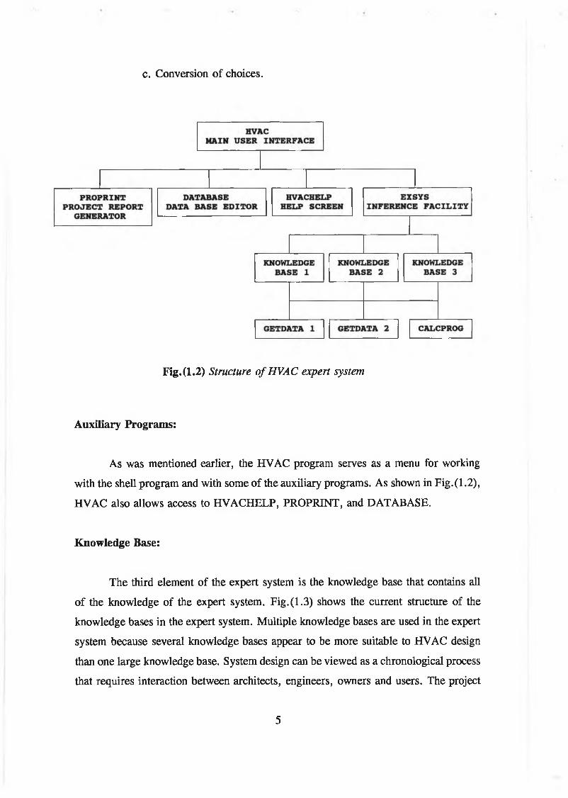
Fig.(1.2) shows the first part which is the structure of the HVAC design expert system
[5]. At the top level is the HVAC main user interface. This program was written
specifically to interact with the selected shell and to serve several functions.
First, HVAC is an interactive menu that allows the user to work with the shell
program and with some auxiliary programs by selecting options from the menu screen.
HVAC’s second and most important function is its project file manipulation. The
objective is to have a data file for each active design project. Project file manipulation
consists of three separate functions:
a. Configuration of active project file.
b. Removal of outdated data.
4
c. Conversion of choices.
Fig.(1.2) Structure o f HVAC expert system
Auxiliary Programs:
As was mentioned earlier, the HVAC program serves as a menu for working
with the shell program and with some of the auxiliary programs. As shown in Fig.(1.2),
HVAC also allows access to HVACHELP, PROPRINT, and DATABASE.
Knowledge Base:
The third element of the expert system is the knowledge base that contains all
of the knowledge of the expert system. Fig.(1.3) shows the current structure of the
knowledge bases in the expert system. Multiple knowledge bases are used in the expert
system because several knowledge bases appear to be more suitable to HVAC design
than one large knowledge base. System design can be viewed as a chronological process
that requires interaction between architects, engineers, owners and users. The project
5

goes from pre-feasibility to pre-design to facility analysis, system selection, and so on.
Invariably the results of one phase are inputs to the next phase. A further problem with
a single knowledge base is that even minor changes in input data would require running
the entire knowledge base, thus reconsidering every possible outcome and taking up
valuable time.
The knowledge bases shown in Fig.(1.3) are arranged in the normal
chronological order in which they would be used. The main menu of the HVAC user
interface contains the pre-feasibility study knowledge base and the facility analysis
knowledge base. The third knowledge selection option in the main menu is the system
design menu. This second menu has the system selection knowledge base, the
equipment selection knowledge base, and the controls selection knowledge base . The
current chronological flow is, therefore, pre-feasibility study, facility analysis, system
selection, equipment selection, and finally controls selection. The complete expert
system will require several other knowledge bases, many of which will have to interface
with design graphics. The purpose of the knowledge bases listed in Fig.(1.3) is to
demonstrate the feasibility of the expert system.
Fig. (1.3) Knowledge base structure
6
1.2.3 C o m p u t e r A i d e d E n g i n e e r i n g ( C A E ) f o r HVAC s y s t e m d e s i g n:
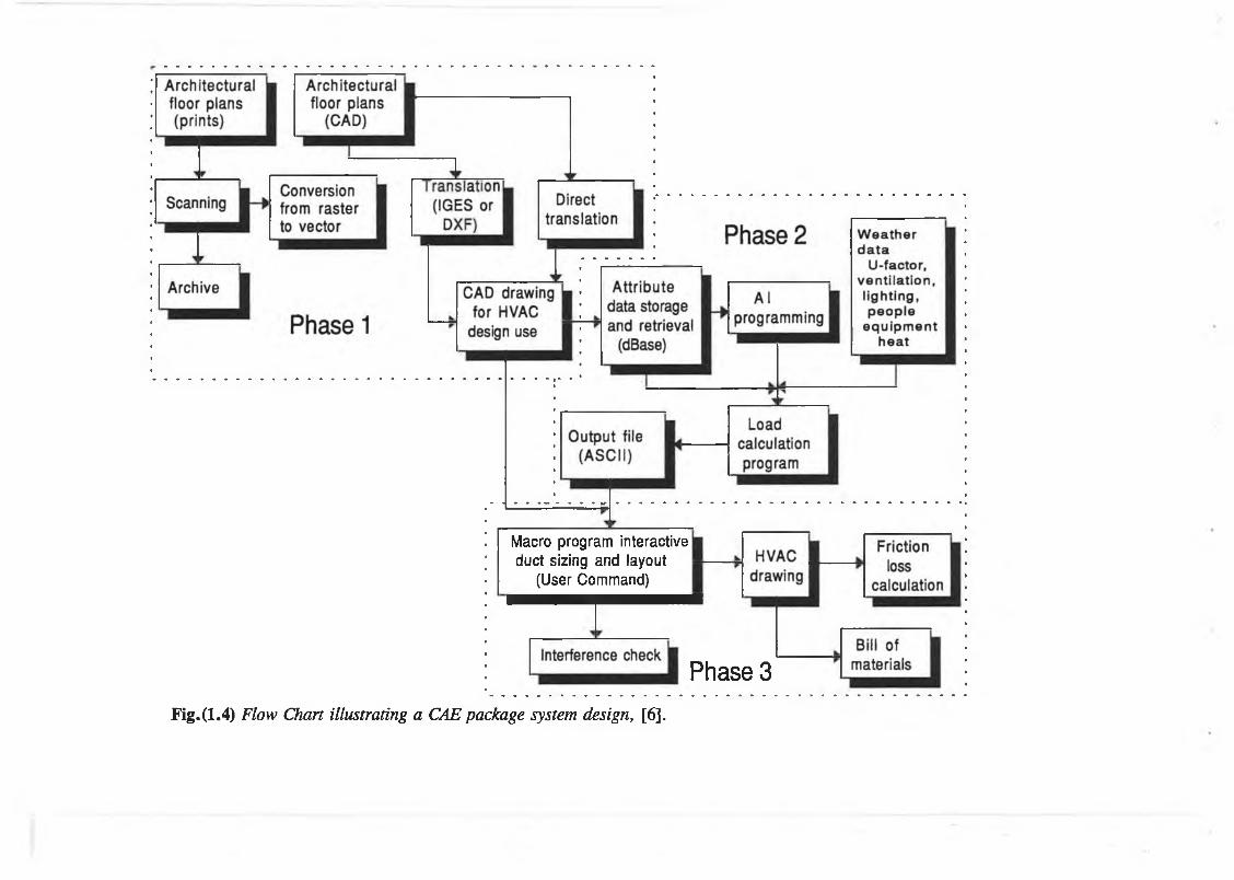
Many of the design tasks now done manually can be incorporated into an
integrated and automated CAE program package. Lam [6] developed another HVAC
expert system shell using Computer Aided Design (CAD) systems. The objectives of
his work ware to explore the possibility of a CAE package that would integrate and
automate engineering and drafting for the HVAC industry and to develop a program
flow chart for a generic process.
If the building process is examined, we find that from conceptual design to final
building turnover to the clients a lot of tasks are done manually by the HVAC engineer.
If the amount of time for these manual tasks is minimized during the design stages, the
client can save money and the HVAC consulting engineer can make more profit. With
this in mind, we can identify the tasks normally done manually or done independently
on a PC by the HVAC design engineer. If we can provide a parallel CAE facility to
replace these tasks, we can establish the criteria for a CAE program. The flow chart,
in Fig.(1.4) shows the suggested flow chart for the entire CAE process by Lam [6].
The flow chart depicts an integrated and automated process, from scanning to final
product (HVAC drawing), that is parallel to how a typical HVAC engineer would work
normally. Development of the CAE package can be divided into three phases. Each
phase should be able to function individually and should have hooks or interface left
open for the next phase:
Translating CAD Graphics:
The translation of graphics using Initial Graphics Exchange Standard (IGES) or
Drawing interchange format (DXF) between different CAD systems is limited to
graphic data only. Any associated data or attributes may be lost during the translation
process. It would probably take another research just to discuss the different types of
CAD translation software and their pros and cons. However, we can summarize the
current status of this topic as that there are a number of translation methods (IGES,
DXF, etc.) [7], which are a standard for graphic data exchange which is imminent.
7
Macro program interactive duct sizing and layout
(User Command)
Phase 3
Fig. (1.4) Flow Chart illustrating a CAE package system design, [6].
The best way to accomplish this is to write short micro programs. Micro
program languages, such as User Commands in Intergraph, Autolisp in AutoCAD [8]
can be used. Using micro programs will automate some of the cleanup and editing
required after an IGES transfer, such as graphic group regrouping or block "exploding"
or reblocking. External FORTRAN programs are also supported by some CAD
software, such as Intergraph and Autotrol.
Calculation of HVAC loads:
Assuming most of the graphics and associated data are intact after the
translation, external or micro programs can be written to read, retrieve and store the
necessary attributes (thickness of wall, window sizes, area, hight of building and
building partitions, etc.) in a database. One can also use DATABase in AutoCAD [7]
to accomplish data retrieval.
This database is then interpreted so that it can be understood and utilized by a
third-party HVAC load calculation program from companies such as APEC, Elite,
Carrier, Trane, or by a program that can be developed in-house.
The interpretation of the attribute database will require some programming in
artificial intelligence (AI) language. Assumptions and Knowledge-bases should be
developed and inputted automatically during this stage so that all the attributes of the
building model can be understood and utilized in the load or energy calculation.
With a minimum of the input from HVAC engineer, the load calculation will be
carried out automatically using the database and local weather data files. The program
output will be stored in an output file, preferably an American Standard Code for
Information Interchange (ASCII) file to facilitate the next automated task.
The duct program :
This program should also be written in the micro language that is provided with
9

the CAD software( e.g., User commands with Intergraph). An interactive approach is
proposed in lieu of the batch-processing approach because it is more logical to set up
the program so that it works the same way the HVAC engineer normally works. It
Should be appropriately divided into the following sections:
* Interactivity asking where the user identifies the starting and ending
points of the sections of the duct system layout.
* By using the Darcy-Weisbach and Colibrook [7,8,9,10,11] equations and
the ASCII files from the load calculation, the duct work will be sized
automatically.
* Friction loss in each section of the ductwork will be checked against the
user input limiting velocity and allowable ceiling clearance.
* Dimensions of each section of the ductwork will be stored in the
database for material take-off purposes.
Here is how the program would work. The program would initially load the
scanned and translated image of the architectural floor plan on the personal computer
(PC) screen. It would prompt the user to input the friction loss factor per 100 ft of the
duct, the limiting velocity, the roughness of the sheet metal used, and the allowable
ceiling clearance dimension.
The program would then prompt the user for the start point of the duct system
layout. As soon as this was entered, the output file from the load calculation would be
read, and the air flow rate (cfm, m3/hr) would be used to calculate the duct size. It
would then prompt the user for the end point to this section of the ductwork, and the
ductwork would be drawn on the screen accordingly. Fittings such as elbows,
transitions, dampers, and the turning vanes would be added automatically, based on the
coordinates of the last option, the previous duct size, the direction of the next point, and
the flow rate.
The initial inputs, such as the limiting velocity and the ceiling clearance, would
act as check figures to round off the duct height/diameter to fit in the ceiling void. This
10

interaction would be carried out until the user entered quit or reset. All the necessary
data for friction loss calculation and material takeoff would be saved in a database while
the interaction was being carried out.
1.2.4 HVAC Programs:
There are mainly two sectors of development for HVAC systems design. The
academic (research) sector, including ASHRAE, DOE, NBS, CIBSE companies [6,12], and numerous universities in the world who are actively involved in the development
of HVAC load calculation and energy simulation programs. Established programs, such
as BLAST, DOE2.1, TRAP, ESP, etc., have been available for many years. The
commercial sector also has many engineering calculation programs available; Trane
[13], Elite Software [14,15,16], Carrier [13], Hevacomp [17], and APEC have been in
the market for years.
On the other hand, the CAD software industry, AutoCAD, has AEC
(Architectural, Engineering and Construction) mechanical and architectural packages;
however, they are basically drafting packages that use menus and symbol libraries.
Intergraph has the PDS package that contains a HVAC module. PDS is an integrated
plant design program that includes practically all engineering disciplines; however, it
is a VAX-based system, and thus its cost is high. Computer vision has its Personal
Architect and Personal Designer packages; again, they are basically drafting packages.
Other CAD software vendors, such as Autotrol, CADAM, CADkey, CADvance,
Drawbase, FastCAD, and VersaCAD, are most likely involved in the development of
specialized packages for the AEC industry.
All of the programs mentioned above are excellent products of many years of
development. However, they all work independently of each other. Integration of these
programs into CAE is still in its infancy. Details of some of these packages are as
follows;
Elite Software programs:
11
Elite Software developed various programs [14,15,16] for HVAC design, some
of these programs are listed below:
QHVAC - Simple Commercial HVAC Loads: This program [14] calculates the maximum
heating and cooling loads for commercial buildings. QHVAC allows 50 zones which
can be grouped into 10 air handlers. The program automatically looks up all cooling
loads and correction factors necessary for computing loads.
DUCT SIZING: This program calculates duct sizes using either the static regain, equal
friction, or constant velocity methods.
U-FACTOR: This program calculates the conductivity factor (U-factor) of walls and
roofs.
PSYCHART: The PSYCHART [16] program displays the psychrometric chart on the
computer screen. It displays numerical values of all properties of the moisture air for
any selected point, and all the processes such as heating, cooling, humidification,
dehumidification, and mixing are displayed on the screen.
SPIPE - Service Supply Pipe Sizing: calculates the pipe size for hot and cold water
domestic water supply systems in both residential and commercial buildings using
ASHRAE and ASPE procedures. It uses the Hazen-Williams equation to determine the
pressure drop due to friction for a particular pipe size. Water velocity is calculated by
first determining the expected gpm flow rate and then dividing by the pipe cross
sectional area.
There are also other programs developed by Elite Software such as SHADOW,
CHVAC, HTOOLS [15] , ENERGY, etc.).
TRANE Programs [13] :
The following summary describes the programs developed by TRANE using
12

Trane’s TRACE and other CDS computer programs to calculate HVAC loads. They use
network and personal computers, some of these programs are explained below:
Load Design: This program can be loaded on a microcomputer and is based entirely on
ASHRAE algorithm and actual hour by hour weather tape data. All ASHRAE
wall,floor, roof, and slab data are preloaded into the program. They put both of the
ASHRAE [7] methods, total equivalent temperature difference (TETD), and the cooling
load temperature difference (CLTD) for the calculation of the cooling load.
Energy Analysis program: This building energy analysis program is designed to
calculate hourly loads throughout the year. It calculates the yearly energy consumption,
operation costs, and equipment payback.
CAD Interface with Ultra Edition Design and Duct Design: This system integrates the
entire computer-aided drafting and computer-aided design (CAD) processes. With the
Trane CDS software and Sigma Design or AutoCAD system, the user can start with
initial calculations and finish with final schedules. The user can begin with an
architectural outline of the building, and the system measures lengths and areas of
zones, generates reports, and provides input for the Ultra Edition Load Design
program. This information is then fed into the Duct Design program, completing the
duct design process.
Veratrine (Static Regain) Duct Design: With this duct-sizing program, the user inputs
the duct layout in simple line-segment form with the cubic feet per minute for the zone,
the supply fan value of cubic feet per minute, and the desired noise criteria (NC) level.
The program sizes all the ductwork based on an iterative static regain procedure
and selects all variable air volume (VAV) boxes when desired. It identifies the critical
path and downsizes the entire ductwork system to match the critical-path pressure drop
without permitting zone NC levels to exceed design limits.
The output of this program is an efficient, self-balancing duct design. It gives
13
I

the designer a printout of the static pressure at every duct node, making trouble
shooting on the job site earier. The program will estimate the duct system and print a
complete bill of materials, including schedules.
Equal-Friction Duct Design: This program produces the total pressure as well as the
pressure drop for each trunk section. The output also includes duct sizes, air velocity,
and friction losses. The program can be used for fiberglass selection as well.
The program will calculate the metal gauges, sheet-metal requirement and total
poundage and provide a complete bill of materials.
DOE-2 PROGRAMS [18]:
This program developed by the U.S. Department of Energy, is based upon the
ASHRAE proposals and consists of four main programs:
LOADS, SYSTEMS, PLANT, and ECONOMIC [19]. The LOADS program computes
the transient response of the building fabric to produce hourly thermal loads in each
space. These thermal loads are then used by the SYSTEMS program, together with the
characteristics of secondary systems to calculate the loads on the central plant. The
secondary system which may be specified are drawn from a menu of approximately
twenty-five options together with several control schemes and operating schedules. The
energy load data is then used by the PLANT program to simulate the performance of
the central plant, which may be selected from a menu of available options which
includes conventional heating and cooling equipment together with the cogeneration and
solar system. The ECONOMICS program provides a life cycle cost analysis to estimate
the relative costs of the various options.
1.3 THE NECESSITY OF A HVAC EXPERT SYSTEMS:
The idea of the HVAC expert system is to help the designers in their work and
help them in making decisions beginning from the preliminary phases to detailed design.
14
I

This work provides the procedure and the drawings for the design, it will
considerably reduce man-hours during the whole design process. HVAC-design with
this research will provide:
a. improved productivity.
b. increased design quality.
c. design standard and regulations that are dynamically useable.
d. design changes that can be controlled and managed.
e. several quality/cost alternatives for customers to choose from.
f. a system that accumulates design knowledge.
1.4 OUTLINE OF THE THESIS:
The objective of the current research is to develop a number of comprehensive
packages which can be used to produce the HVAC systems design for scientific and
commercial building. These packages are HVACSYS which are designed as a pull-down
menu for calculating the HVAC loads, and to display the results and print them out.
HVACCAD is designed by customizing AutoCAD Software to be used to give HVAC
systems drawings. These packages should give the results for the building of HVAC
systems.
The developed knowledge based system should be capable of achieving the
optimum system design for all applications, and of being used efficiently by HVAC
designers. It must therefore be relatively simple and straight forward to use and capable
of running on a personal computer.
The research work carried out in accomplishing the above tasks has been laid
out as follows;
• A review of various procedures for HVACSYS and HVACCAD package
commands is given in chapter two. These procedures give an illustration of the
two packages and their subroutines.
15

• Theoretical analysis and description of HVAC load calculation steps are
presented in chapter three. Chapter three also includes a psychrometric chart
subroutine to present the processes of air conditioning and get the properties of
the moist air at any assumed case. The U-Value subroutine calculation steps are
also presented in this chapter.
• Customizing AutoCAD menu for HVAC systems programs as "Pipework" to
calculate the pipes sizing, "Ductwork" for calculating the duct size, and
"Psychart" programme are described in chapter four.
• Case study of the developed package and discussion for comparing the results
of the example with another commerical package are presented in chapter five.
• Finally the conclusion of the research and recommendations for further work
are given in chapter six. The list of references and appendix of U-value materials
data are presented at the end of this thesis.
16
CHAPTER TWO
DESCRIPTION OF HVAC SYSTEM DESIGN SOFTWARE
2.1 INTRODUCTION;
For a typical design process, the HVAC consulting engineer normally gets a set
of prints from the architect. He then gets either a draftsman to trace the architectural
floor plans on vellum or mylar or a CAD operator to copy the floor plans into a
diskette with the help of CAD software such as AutoCAD or Computervision. If the
architect happens to use CAD and his software is different from that of the HVAC
engineer, the engineer must try to translate the architectural CAD drawings so that his
CAD system can understand them. If the translation is not successful then the HVAC
engineer pulls out his scale and starts calculating floor areas, window sizes, wall
thicknesses, etc., from the architectural floor plans. He then refers to a handbook or
the manufacturer’s data and gets the weather data, U-values, ventilation rates, exhaust
rates, equipment, appliance heat losses, lighting wattages, and so on. With these data
on hand, he starts to do the load calculations, either manually or on a PC.
After completing the calculations, the HVAC engineer starts the duct sizing,
pipe sizing, air, water friction loss calculation and equipment selections. If the
examining of duct sizing process is limited, the HVAC engineer usually does it
manually by sketching a one-line duct layout and using a ductulater or friction chart to
size the ductwork. There are duct sizing computer programs on the market, but the
data-input process is laborious. Most HVAC engineers prefer to use the old faithful
Ductulator.
The HVAC engineer then passes the duct layout sketch to a draftsman and the
draftsman tries to produce a proper, scaled, double-line drawing on a drawing board
or a CAD workstation. Ordinarily, the draftsman does not or can not check whether the
duct layout is correctly designed or check the interferences with other building services
17
facilities. An interference check is usually done manually by a facility peer-check or
office-check within the consulting firm.
If the project requires it, the HVAC engineer may have to determine the
material requirement for HVAC system. Again, this is normally done manually by
using a scale to get the length and the size of the ductwork, and by counting the number
of fittings, deffusers, dampers to come up with a tabulated bill of materials.
This chapter gives a general review of the development in the field of HVAC
knowledge based (KB) system. This research attempts to introduce developing the
computer package HVACSYS based on such developments. This generalized package
will evaluate the performance of heating, ventilation and air conditioning design. The
package is composed of a number of computer codes which are based on minimum
input data by the user such as the information on buildings ( uses, constructions,
dimensions, occupants, etc.) and the weather.
HVACCAD is designed by customizing AutoCAD software, this gives the user the
opportunity to work on AutoCAD as a HVAC drawing package. It is used to give all
HVAC systems drawings (pipework, ductwork), and to workout all air conditioning
processes on a psychrometric chart.
The output of the developed packages produce the final HVAC system design
of the building which include:
1 - HVAC system engineering drawings.
2 - List of materials and their quantities.
3 - Individual and total component costs.
4 - Reports of the HVAC loads can be either viewed on the screen or
printed together with the inputs entered by the user.
2.2 SYSTEM CONFIGURATION:
The function of this system, as mentioned above, is to design the HVAC system
18

starting from getting the architect’s plans of the building until producing the final
HVAC system drawings. The steps of using this system are shown in Fig.(2.1) and
explained as follows;
1. Building drawings are recieved from the architectural engineer by elctronic mail
through computer network or on storage disk. These drawings contain the following
information:
a. Architect’s plans of the building.
b. The type and quantities of the material used in the building construction.
c. The building furniture and the number of the people who are going to occupy
the building.
HVACSYS User Interface
Fig. (2.1) The structure o f the developed knowledge based system
2. Enquiries from the system user whether special conditions are required inside the
building such as temperature, humidity or air purity.
19

3. Getting the weather data from DATABase files (outside temperature, outside
humidity, wind direction and magnitude, CLTD, Solar Heat Gain Factor (SH G F), )
for the calculation using HVACSYS package.
4. HVAC loads and system calculations are carried out by the routines developed
within HVACSYS package to produce ASCII files and DXF files for HVACCAD
package.
5. HVACCAD package access the material, standard components and equipment
records in the DATABase and retrieve information such as power, prices, volume, etc..
6. The data in the ASCII files produced by HVACSYS for calculation and drawing
HVAC system, are accesed by routines in HVACCAD for further analysis and also for
reading DXF files to display the drawings through HVACCAD routines.
7. Technical reports which may include input data for the HVAC loads can be displayed
on the screen or printed out.
8. HVACCAD produces HVAC systems drawings which includes all the design
information in detail such as piping, and ducting systems.
2.2.1 Hardware configuration:
The research described in this thesis has been carried out using a microcomputer
connected with complete hardware as follows;
1. A 286 personal computer with Math Coprocessor, 1.028MB of RAM, and
storage consisting of a single 40MB hard disc, and floppy drives (5 V2", 3 V2").
A microcomputer was selected for this research because the intent is to develop
a PC based system which will also permit the use of AutoCAD software for
drawing. The selection of the hardware is very important for the ease of work,
and the user can run more than one software at the same time. For example, in
20
this research the user working in AutoCAD package can run other software like
the developed package (HVACSYS) and return to AutoCAD at any time.
2. A colour monitor with EGA graphic display.
3. A mouse (GM-F303) used as a digitizer for AutoCAD.
4. A printer (Star LC-10) for report printout.
5. A plotter (Hewlett Packard DraphPro DXL) for the drawing output.
2.2.2 Software configuration:
The software used in this development are divided into two categories;
1 . The commercial Package:
a. AutoCAD, 2D and 3D package release 10.
b. Quick Basic Programming Software.
2. Inhouse developed packages:
a. HVACSYS package.
b. HVACCAD package by customizing AutoCAD.
2.3 HVACSYS PACKAGE DESCRIPTION
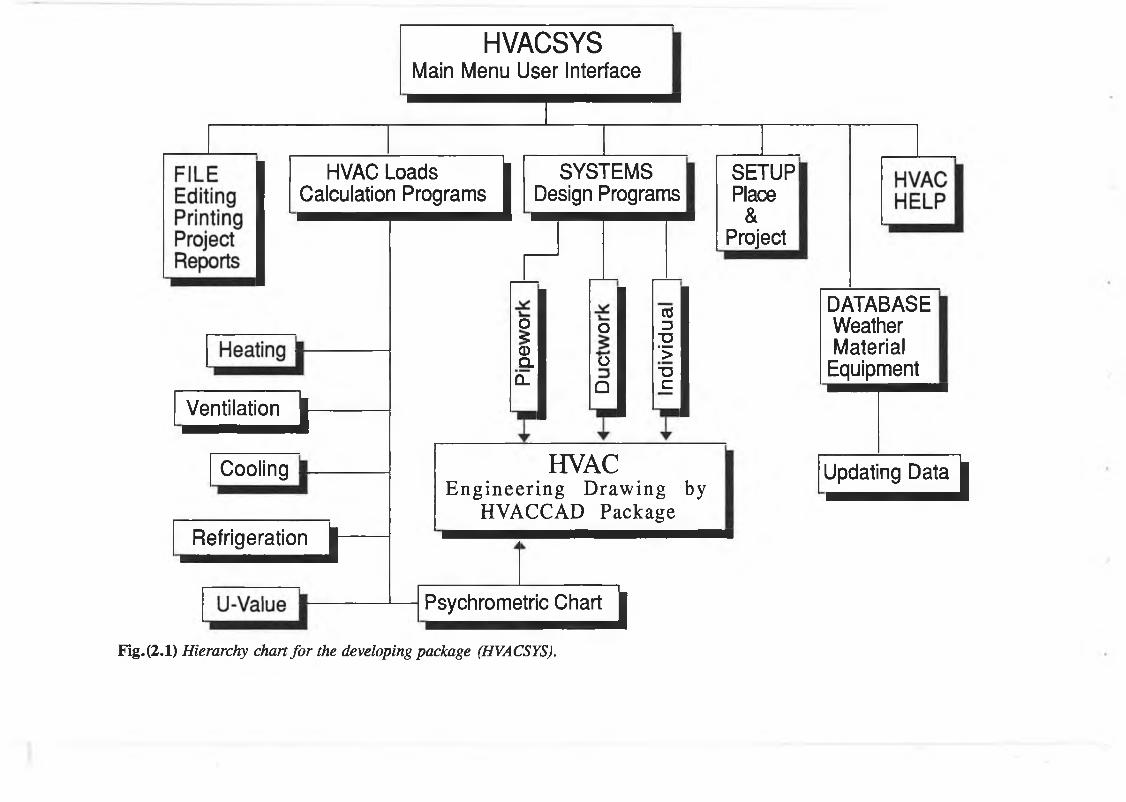
Fig.(2.2) shows the flow chart of the developed package (HVACSYS), which
is totally pull-down menu driven, the master menu being the first and central menu that
will branch to all other menus. These menus will make the program extremely user
friendly even to the first time user. The input data is requested via a menu screen that
is accessed through the master menu. The descriptive titles for input fields will appear
on the monitor. The output from the programs are connected to the AutoCad Package
by customizing its menu to HVAC system menu ( HVACCAD ) to perform the final
engineering drawing.
The developed package ( HVACSYS ) is used to perform all the design of the
HVAC system of Buildings. It contains a number of programs which the user can deal
with easily to get the characteristics used by the HVAC designer.
21
HVACSYSMain Menu User Interface
HVAC Loads Calculation Programs
Ventilation }Cooling
^e frig e ra tio r^J -
]
SYSTEMS Design Programs
SETUP! Place &
Project
o<:0)CLO.
O
OQ
COD■g'>T3c
HVACEngineering Drawing by
HVACCAD Package
Psychrometric Charti
DATABASEWeatherMaterial
Equipment
U pdatinç^at^
Fig. (2.1) Hierarchy chart fo r the developing package (HVACSYS).

2.3.1 HVACSYS M ain M e n u :
HVACSYS is an user interface which consists of six pull-down menus for easy
use by any customer of the software. The interactive computer programs have been
written in basic language using Quick Basic Compiler. It is displayed like any other
software but with different command facility as follow;
F i l e S y s t e m s D a t a b a s e S e t u p H e l p
To activate the menu bar, one can use the keyboard to select the desired option.
2 . 3 . 2 F I L E COMMAND:
This option has a menu bar of five commands as follows:
SaveP r i n tD i r e c t o r yD o s S h e l lQ u i t
Open c o m m a n d : This retrieves a document from the disk which represents a file of any
HVAC project, and copies it on the screen for editing. The user can open several types
of files by using the Open command on the File menu, Only ASCII files can be edited
on the screen.
To open a file:
1. From the File menu, the user has to choose Open. Then the Open dialogue
box appears.
2. The user then has to type the filename required and press the Enter key. If
23

the file he wants is not on the current drive or directory, he has to type the path
as part of the filename.
Save c o m m a n d : This saves the current document on the screen to a hard disc or a
floppy disc. The dos filenames can have up to eight characters plus an optional three-
letter extension.
To save a file:
1. From the File menu, the user has to choose save command, then the Save
dialogue box appears.
2. In the File name box, the user has to type a name for the file. If the user
wants to save the file on a different drive or directory, he has to type the path
as part of the filename.
Print C o m m a n d : To print the current document on the printer, and put the printed
document in paginated papers, the user must have a printer connected to or redirected
through the LPT1 printer port
To print a file:
- From the File menu, the user has to choose the Print command, the print
dialogue box appears, to allow the user to adjust the paper and to ensure the
printer is on.
Directory c o m m a n d : This command displays a list of files, by selecting this option the
screen will display a list of all the files that match the given filename template.
DosShell C o m m a n d : This command allows the user to exit temporarily from the code
and return back.
Quit C o m m a n d : This command exits the package to dos prompt after giving the user
a chance to save the current document. The ESC key can cancel the exit.
2 . 3 . 3 P R O G R A M command:
This command takes the user through a submenu which contains many important
programs to be used by any HVAC systems designer, this submenu has six options, as
follows;
24
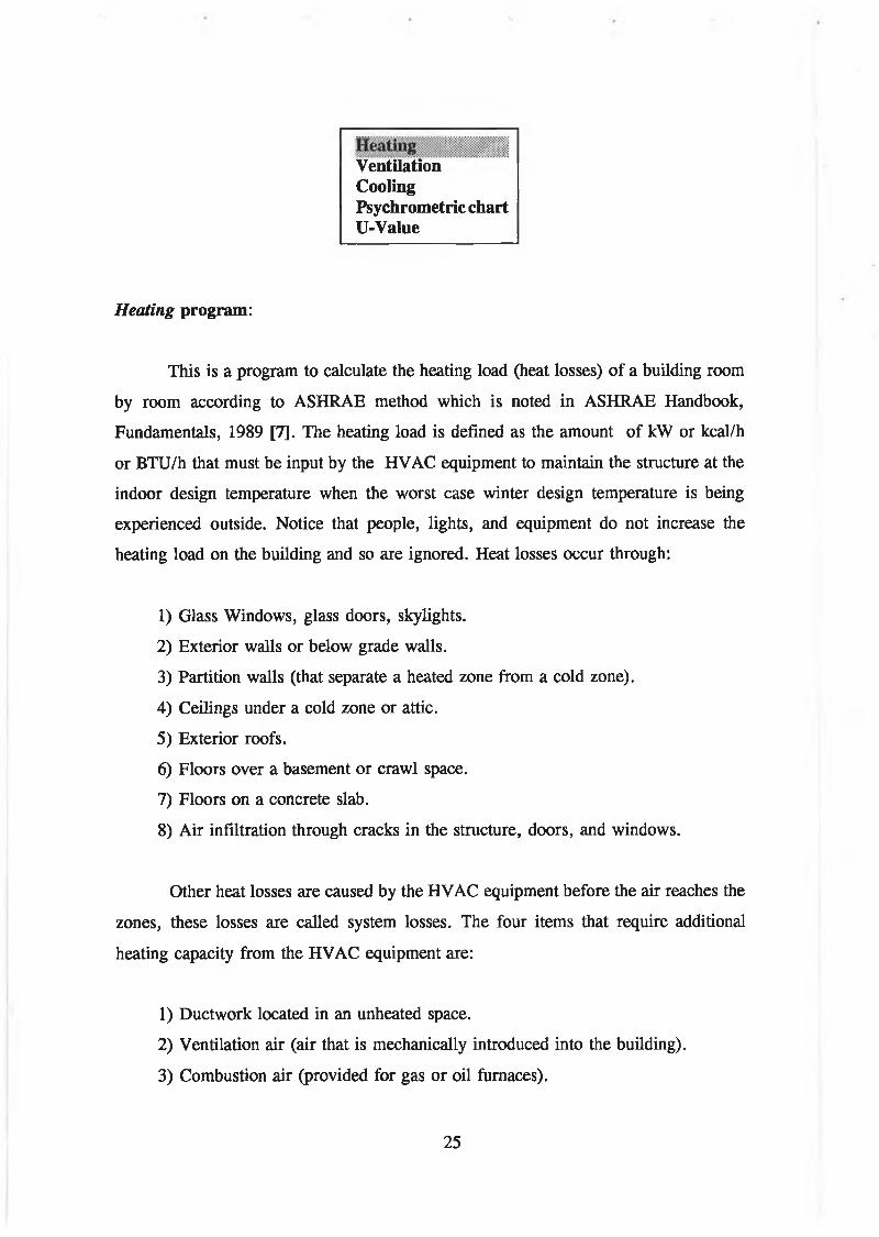
V e n t i l a t i o nC o o l i n gP s y c h r o m e t r i c c h a r t U - V a l u e
Heating p r o g r a m :
This is a program to calculate the heating load (heat losses) of a building room
by room according to ASHRAE method which is noted in ASHRAE Handbook,
Fundamentals, 1989 [7]. The heating load is defined as the amount of kW or kcal/h
or BTU/h that must be input by the HVAC equipment to maintain the structure at the
indoor design temperature when the worst case winter design temperature is being
experienced outside. Notice that people, lights, and equipment do not increase the
heating load on the building and so are ignored. Heat losses occur through:
1) Glass Windows, glass doors, skylights.
2) Exterior walls or below grade walls.
3) Partition walls (that separate a heated zone from a cold zone).
4) Ceilings under a cold zone or attic.
5) Exterior roofs.
6) Floors over a basement or crawl space.
7) Floors on a concrete slab.
8) Air infiltration through cracks in the structure, doors, and windows.
Other heat losses are caused by the HVAC equipment before the air reaches the
zones, these losses are called system losses. The four items that require additional
heating capacity from the HVAC equipment are:
1) Ductwork located in an unheated space.
2) Ventilation air (air that is mechanically introduced into the building).
3) Combustion air (provided for gas or oil furnaces).
25
4) Return-air Plenum.
The results can be displayed on the screen or printed. In addition, the results are
saved in files, these files are then recalled by HVACCAD interface to give the system
plans.
Ventilation p r o g r a m :
The quality of the air inside a building, i.e, its temperature, moisture level,
purity, movement and oxygen content, affects the well-being of those who work, live
or visit the building. Air becomes stale or contaminated by the use made of the space.
People at work decrease the relative proportion of oxygen in the air and will give rise
to body odours, moisture and heat. Tobacco smoke, at best an irritant to non-smokers,
may increase the risk of their developing lung cancer. Chipboard furniture and carpet
may give off formaldehyde, and other furnishings produce dust and fibres. In addition
to calculating the heating loads of some places like workshops, basements, labs, etc.,
using the last program, we need to ventilate these places by fresh air. Ventilation is a
return-side load and is time dependent. It is caused by outside air that is deliberately
introduced into the HVAC unit. The cold (or hot) air that enters the HVAC unit is
heated (or cooled) before it reaches the room. Therefore, it is a system load, and is not
calculated for individual zones. This program calculates the heating loads which cover
the ventilation loads. However, the ventilation system has been designed in such a way
that it is separated from the heating system.
Cooling p r o g r a m :
This is the main program for calculating the cooling loads of the building, it
calculates the loads room by room.
The cooling load (or heat gain) is defined as the amount of kW or kcal/h or BTU/h
that must be input by the HVAC equipment to maintain the structure at the indoor
design temperature when the worst case summer design temperature is being
26

experienced outside. There are two types of cooling loads; sensible and latent. Sensible
cooling refers to the dry bulb temperature of the structure. Latent cooling refers to the
wet bulb temperature of the structure. In the summer, humidity is a factor in the
selection of the HVAC equipment and the equipment must be sized to handle the latent
load.
The sensible cooling load occurs through:
1) Glass Windows, glass doors, skylights.
2) Sunlight striking windows, skylights, or glass door and heating the zone.
3) Exterior walls.
4) Partition walls (that separate a heated zone from hot zone).
5) Ceilings under an attic.
6) Roofs.
7) Floors over an open crawl space.
8) Air infiltration through cracks in the building, doors, and windows.
9) Fluorescent lights.
10) People in the building.
11) Equipment operated in the summer.
12) Draw-through fan located in the air stream.
Notice that below grade wall, below grade floors, and floors on concrete slabs
do not increase the cooling load on the structure and are therefore ignored.
Other sensible heat gains result from the HVAC equipment before the air
reaches the zones, these gains are called system gains. The four items that require
additional sensible cooling capacity from the HVAC equipment are:
1) Ductwork located in an unheated space.
2) Ventilation air (air that is mechanically introduced into the building).
3) Blow-thru fan located in air stream.
4) Retum-air Plenum.
27
The latent cooling load occurs through:
1) People.
2) Equipment, pools, indoor fountains, etc.
3) Air Infiltration through cracks in the building, doors, and windows.
Other latent heat gains are from the HVAC equipment before the air reaches the
zones, these gains are called system gains. The item that requires additional latent
cooling capacity from the HVAC equipment is:
- Ventilation air (air that is mechanically introduced into the building).
The output will be sensible load, latent load and the flow rate of supply air and
its temperature, or the capacity of the fan coils depending on the chosen system.
Refrigeration p r o g r a m :
This program calculates the refrigeration loads for any sized cooler, freezer,
warehouse, walk-in unit, etc. Freezer temperatures can be as low as -50 °C. The
refrigeration loads include transmission loads, internal loads, product loads, and
infiltration loads. Allowance is made for compressor run-time, fan heat, a safety factor,
product pull-down time, and loads occurring in the box such as forklifts. The program
uses dynamic, on-screen calculations so that the user can instantly see the effect of each
item on the loads. The program comes with built-in libraries for products, container,
coils, compressors and weather data. These libraries can be modified by the user to
update the information and are stored permanently by the program. The program
produces an extensive set of reports, including a summary listing of each load and its
percentage of the total.
Psychrometric chart p r o g r a m :
The means for simulating the principles of air-conditioning processes are done
28

in this program. It is composed of:
i) estimating the relevant properties of atmospheric air (Psychrometric properties),
ii) predicting the behaviour of air when undergoing constant-pressure mixing, heating,
cooling, humidification and dehumidification processes.
U-value p r o g r a m :
The calculation of HVAC loads begins with the determination of U-values,
which are overall heat transfer coefficients. U-values are calculated by taking the
reciprocal of R-values and the conductivities of the materials. It is a complete menu bar
program which the user can execute separately or as a subroutine in the last program.
2.3.4 SYSTEMS command:
This command gets the user through a menu bar which is the second important
menu bar, it contains three system option:
Pipewor*kD u c t w o r kI n d i v i d u a l
Pipework o p t i o n :
This option gets the user through a program which has four subroutines for the
pipe size calculations.
1) Hot and cold water pipe sizing subroutine: This is the main subroutine to calculate
the optimum pipe size for hot and cold domestic water supply systems in scientific,
residential, and commercial buildings using ASHRAE procedures. Depending on the
computer’s memory, the system can contain details of a number of pipe sections. This
29

program also performs a system analysis that produces reports that list, pressure drops,
required pressure flow rate, and water velocity at any design system.
2) Refrigerants pipe sizing program.
3) Gas pipe network program; this is not included in this thesis.
4) Steam pipe network program; this is not included in this thesis.
Ductwork o p t i o n :
This option gets the user through a duct size program which comes in two
versions:
1) The static regain, equal friction, and constant velocity method.
2) The only equal friction, and constant velocity method.
The calculation of duct sizes are printed on the basis of both round and
rectangular cross-section. The program can handle all-air systems which are:
a) Single-zone constant-volume system.
b) Single-zone constant-volume system with reheat.
c) Multizone system.
d) Induction unit system.
e) Variable-air-volume system.
f) Dual-duct system.
Individual system o p t i o n :
This program deals with Direct Expansion (DX) systems, and is divided into
three options in a pull-down menu;
i) Window type air-conditioning units.
ii) Split system units.
iii) Central DX coils system.
30
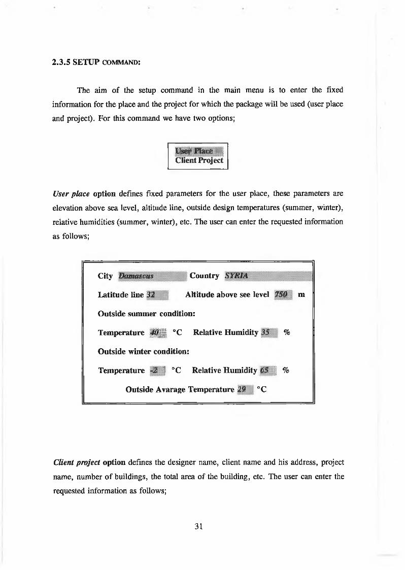
2.3.5 SETUP c o m m a n d :
The aim of the setup command in the main menu is to enter the fixed
information for the place and the project for which the package will be used (user place
and project). For this command we have two options;
U s ts j* P ia c fe C l i e n t P r o j e c t
User place o p t i o n defines fixed parameters for the user place, these parameters are
elevation above sea level, altitude line, outside design temperatures (summer, winter),
relative humidities (summer, winter), etc. The user can enter the requested information
as follows;
C i t y Damascus C o u n t r y SYRIA
L a t i t u d e l i n e 32 A l t i t u d e a b o v e se e l e v e l 750 m
O u t s i d e s u m m e r c o n d i t i o n :
T e m p e r a t u r e § ¡ ¡ ¡ ¡ ¡ 1 ° C R e l a t i v e H u m i d i t y %
O u t s i d e w i n t e r c o n d i t i o n :
T e m p e r a t u r e »2 | °C R e l a t i v e H u m i d i t y 6$ %
O u t s i d e A v a r a g e T e m p e r a t u r e 29 ° C
Client project o p t i o n defines the designer name, client name and his address, project
name, number of buildings, the total area of the building, etc. The user can enter the
requested information as follows;
31

C l i e n t A M 'S , Ilamouda A d d r e s s 1 Shantalla Park , ;
C i t y Dublin 9 ■ | C o u n t r y Rep. o f IRELAND 1 1 1 1 1 1
P r o j e c t N a m e H w s# Heating T o t a l A r e a | | | | j m 2
N u m b e r o f B u i l d i n g s t ' H e a t i n g S a f e t y F a c t o r ¡ ¡ | %
B u i l d i n g O p e n i n g H o u r § | S e n s i b l e S a f e t y F a c t o r | | f %
B u i l d i n g C l o s i n g H o u r M L a t e n t S a f e t y F a c t o r ¡ ¡ i f %
Designer ¡p t . A ltihban | f | | | Address School o f Mech. & Manu. Eng.
2 . 3 . 6 D A T A B A S E c o m m a n d :
Each program for the design of any HVAC system needs to build up a database
of;
1) building materials to use for calculating the U-value,
2) weather conditions for calculating the heating and cooling loads,
3) equipments with their capacities, types and prices.
The purpose of database is also to let the user enter his own data and update the
old data. Any selection of this command goes to menu bar of three options which is
displayed as follows:
M a t e r i a !W e a t h e rE q u i p m e n t
Material o p t i o n gets the user through a list of materials which includes building
structure materials especially those used for U-value calculation, and HVAC
components like pipes, duct, and their fittings ( elbows, tees, flanges, etc.)
32

Weather o p t i o n contains all the weather data schedules list used for calculating the
cooling loads that are mentioned in the ASHRAE Handbooks [7,20-23] and ASHRAE
Standard [23].
Equipment o p t i o n gets the user through a list of equipment which can be used in
HVAC systems. This is like a catalogue of equipment with their capacities and their
prices. The user can update the prices and increase the number of equipment.
2.3.7 H E L P COMMAND:
The function of the help command is to guide the user at any time to teach him
how to enter the inputs, to define the procedure sequences, and to use the keys of the
keyboard. Help command menu contains three options as follows:
I n d e xT o p i c
Keys o p t i o n : Gives the user a list of the keys functions in the main menu. By pressing
any of these keys, the user gets to a certain procedure or function command.
Index o p t i o n : This is an alphabetical list of help topics, including the HVACPRO
Keywords. Each term in the index is linked to additional information.
The user can get help by:
1) Choosing the index command from the help menu bar.
2) Pressing the key corresponding to the items first letter.
3 ) Moving the cursor to the item the user wants help on, then pressing F I from
the functions Keys.
33

Topic o p t i o n : Choosing this command displays information on the topic determined by
the current cursor location.
2.4 HVACCAD PACKAGE DESCRIPTION
Common to most engineering tasks is the need to effectively retrieve data,
perform analysis and synthesis based on the data, and store the results for later use. The
results of these operations are eventually documented as drawings, bills of materials,
manufacturing instructions, technical documents and many kinds of reports.
The engineering analysis and synthesis process incorporates a great deal of
know-how which is called expertise. The key to successful engineering drafting
automation is the incorporation of this expertise in a computer.
Traditional CAD systems provide some means to express engineering
knowledge, such as:
* parametric programs.
* graphical Symbols, and
* existing drawings and geometric models.
In addition, some knowledge domain has been implemented by CAD software vendors
in application packages.
Although computer-aided tools provide great potential for automating
engineering design, traditional CAD systems have brought major productivity
improvements mainly to drafting work in the detail design phase.
The HVACCAD package describes customizing the AutoCAD menu to make it
suitable for HVAC system design by adding the commands which the user can use to
collect several HVAC components into a group, forming a composite software system.
The user can then complete the mechanical drawing of the HVAC system, as often as
wanted. The HVACCAD program can also make use of a database information of
34
l
standard components which can be found individually or as an assembly of a group of
components.
The program considers each component of the HVAC system as an entity or a
block. In addition to the mechanical HVAC system drawing, the new package can also
provide drawing database, quantities and bill of materials and equipment.
2 . 4 . 1 H V A C C A D U s e r I n t e r f a c e :
The user interface of H V A C C A D is accomplished by integrating AutoCAD tools
and relational database. H V A C S Y S is closely integrated with the AutoCAD via the
database program and random access files. This means that the user can communicate
with the system via H V A C S Y S and AutoCAD via H V A C C A D . In the H V A C S Y S the
structure of rooms, the system design outputs, spaces and components of HVAC system
are defined as database information. The user can add knowledge and data or update
them in the system whenever required.
The user interface of H V A C C A D consists of three main programs, which are
written in Autolisp programming language. These programs are explained as follows.
2 . 4 . 2 P I P E W O R K PROGRAMME:
This pipe sizing program is for closed and open systems, and for any fluid by
inputting the viscosity and specfic gravity. PIPEWORK is an AutoCAD-based piping
design, layout and drafting program, it is developed to calculate pipe sizing for both
cold and hot water central systems (single pipe, two pipe, four pipe ) and refrigerant
pipe systems. The user inputs the piping layout in simple line-segment form (the start
and end point of each section of pipe) with flow rate for every section of pipe.
PIPEWORK is a 2 D and isometric program which uses the AutoCAD pull-down, ICON
menus fully, and also the screen menu. It adds a new dimension of productivity for
piping and plant design, within the AutoCAD.
35

PIPEWORK is an inegrated program with the HVACSYS package, so that it
gets the data produced by HVACSYS as ASCII files such as flow rates and loads. With
this program the user can draw the piping network with its components (valves, fittings,
hangers, ...), and equipments (boilers, burners, pumps, radiators, unit heaters,
expansion tanks, storage calorifiers, ... ).
After completing the design, the user gets the output which includes:
* line lists, plot plans, orthographies.
* complete bill of materials (including pipe sizing and linear length required,
fitting, equipments).
* Estimated piping system costs of the whole system.
2.4.3 D U C T W O R K Programme:
DUCTWORK is an AutoCAD-based ducting design, layout and drafting
program. It is developed to calculate the size of all ductwork based on an iterative static
regain procedure for all air systems. It identifies the critical path and downsizes the
entire ductwork system to match the critical path pressure drop without permitting zone
noise criteria (NC) levels to exceed the design limits. This is also a 2D program which
uses AutoCAD pull-down, ICON menus fully and also the screen menu. It adds a new
dimension of productivity for ducting and plant design, within AutoCAD.
DUCTWORK is an inegrated program with the HVACSYS package, so that it
gets the data produced by HVACSYS as ASCII files such as flow rates and loads. With
this program the user can draw the ducting network with its components (dampers,
fittings, hangers, ...), and equipments (AHU, fancoils, fans, grills, coils, humidifiers,
condensing units, DX units, filters, diffusers, ... ).
The outputs of this program is an efficient, self-balancing duct design. It gives
the user the following:
* A printout of the static pressure at every duct node, duct sizes, air velocity,
36

frictions losses.
* Plot plans, orthographies
* bill of materials (types, quintities, prices), and estimated costs of the whole
system.
2 . 4 . 4 P S Y C H A R T P r o g r a m m e :
PSYCHART is a display of the psychrometric chart. It allows the user to obtain
the properties of a defined point, and carry out all air conditioning processes (cooling,
heating, mixing, humidification, dehumidification, and general process) which can be
applied on the psychrometric chart.
PSYCHART gives reports of all properties of any point on the psychrometric
chart, and any process defined by the user, and psychrometric chart drawing of the
defined points and processes.
37
CHAPTER THREE
THEORETICAL BASIS OF HVAC LOAD CALCULATIONS
3 . 1 I N T R O D U C T I O N :
HVAC systems are designed to provide control of space temperature, humidity,
air contaminants, differential pressurization and air motion. Usually an upper limit is
placed on the noise level that is acceptable within the occupied spaces. To be successful,
the system must satisfactorily perform the intended tasks. Most HVAC systems are
designed for human comfort as discussed at length in ref. [7,8]. These references discuss
the objective of the HVAC design. Industrial applications may have objectives other
than human comfort. If human comfort can be achieved while the demands of industry
are satisfied, the design will be that much better. However HVACSYS is designed to
cover designs both for commercial buildings (mainly human comfort) and for scientific
buildings including industrials buildings.
One of the cardinal rules for a good, economical energy efficient design is not
to design the total system to meet the most critical requirements of just a small portion
of the total area served. That critical area should be isolated and treated separately, then
if necessary to control the heat transfer to the building (U-Value). HVAC systems
require the solution of energy mass balance equations to define the parameters for the
selection of appropriate equipment. The solution of these equations requires the
understanding of that branch of thermodynamics called "psychrometrics". The modem
designer prefers to use a computer method to calculate HVAC loads, select equipment,
and size piping and ductwork. Especially for large or complex projects, computer
programs are generally the most cost effective and the most recommended. Where one
or more of the following items will probably be modified during the design phase of a
project, computer programs should be used:
38
* Building orientation
* Walls, roof, and floor Construction (overall U-Value)
* Percentage of glazing or glazing area
* Building or rooms sizes
The use of computers in the thermal analysis of buildings and of HVAC systems
has grown from a need to improve the efficiency of the design process. This itself being
influenced by changes in technology and by growing economic pressure. Initially
computer software ware developed for the thermal analysis of buildings, these programs
being used to predict the energy demand within each zone, thus allowing rapid appraisal
of architectural changes and the selection of equipment based on the resulting peak
loads. Programs of this type assume idealised control of the installed plant, the system
maintaining constant conditions in the occupied zone.
However for any project, there are mainly eight programs which should be used
for the complete design. This chapter covers the developed (HVACSYS) package. This
package (HVACSYS) is a set of individual program modules that will interact to enable
the user to enter data, process it and inspect the results in a very organized manner. The
system is entirely menu driven, the master menu being the first and central menu that
will branch to all other menus. The master menu contains the general tasks performed
by the developed package as heating, ventilation, cooling, U-Value, psychrometric chart,
duct size, and pipe size programs which are treated in this chapter. This chapter briefly
explains the different selection of the main programs in the master menu and relevant
theoretical equations and programme execution steps.
3 . 2 H E A T I N G L O A D P R O G R A M M E ;
As a general principle when approaching the question of space heating, it is
desirable that the building and the heating system should be considered as a single
entity. The form and construction of the building will have an important effect not only
upon the method to be adopted to provide heating service, but also upon subsequent re
current energy cost. The amount of heat required to maintain a given internal
39

temperature may be greatly reduced by thermal insulation and by any steps taken to
reduce an unwanted intake of outside air. Large areas of glass impose very considerable
loads upon any heating system and run counter both to the provision of comfort
condition and to any prospect of energy efficient operation.
This program computes heat losses through the building using the ASHRAE
method [7]. The first step in calculating the heating load is to establish the project’s
heating design criteria:
1) Ambient design Weather conditions: temperature, wind direction and wind
speed.
2) Space (indoor) air temperature to be maintained in each space during design
weather condition.
3) Estimate temperature in adjacent unheated spaces.
4) Select or compute heat transfer coefficients (U-Values) for outside wall, glass,
inside walls, non-basement floors, ceilings...etc.
5) Determine the net area of the outside wall, outside roof, glass, roof next to
heated spaces, floors, or next to an unheated area. These determinations can be
made from building plans.
6) Compute heat transmission losses for each kind of wall, glass, floor, ceiling,
and roof in the building by multiplying the heat transfer coefficient (U-Value) in
each case by the area of the surface and the temperature difference between indoor
and outdoor air.
7) Compute heat losses from basement or solid ground floor using the method
mentioned in ASHRAE 1989 Handbook o f Fundamental [7].
8) Compute heat loss from infiltration and ventilation depending on air changes.
9) The sum of the coincidental transmission losses or heat transmitted through the
confining walls, floor, ceiling, glass, and other surfaces, plus the energy
associated with cold air entering by infiltration or the ventilation air required to
replace mechanical exhaust, represents the total heating load.
10) In buildings with a sizeable and reasonably steady internal heat release from
sources other than the heating system, compute and deduct this heat release under
40

design conditions from the total heat losses computed above.
11) The pick-up loads that may be required in intermittently heated buildings or
in buildings using night thermostat setback must be included. Pick-up loads
frequently require an increase in heating equipment capacity to bring the
temperature of structure, air, and material contents to the specified temperature.
12) Material and equipment that may be brought into the building at a temperature
below inside design temperature must be considered.
The heating load is calculated according to all points mentioned in chapter 2,
these procedures are based on ASHRAE Fundamentals [7] which are mentioned above
and also ASHRAE/IES Standard [23].
The winter outdoor design temperature should be based preferably on minimum
temperatures that will not be exceeded for 99 percent of the total hours in the months
of December, January, February (a total 2160 hrs in the northern hemisphere) and the
months of June,July, and August (in the southern hemisphere a total o f2208 hrs) [13].
For energy conservation considerations, the outdoor winter design temperature to be
based on a temperature which will not exceed 79,5 percent of the same total heating
hours. Anyway, the user of this package has the option to choose the outdoor winter
design temperature if there is a special case. Also, there is a recommendation table of
the inside temperatures according to the defined space, and the user has an option to
enter his own temperatures.
3.2.1 Theoretical analysis of heat losses:
Each room in a building is taken in turn and an estimate is made of the amount
of heat necessary to maintain a given steady temperature within the space, assuming a
steady lower air temperature outside. The calculation falls into two parts;
* one relating to conduction through the various surrounding structural surfaces,
walls, floor and ceiling;
* and the other to the heat necessary to warm up to room temperature any
outside air which, by accident of design, has infiltrated into the space.
41
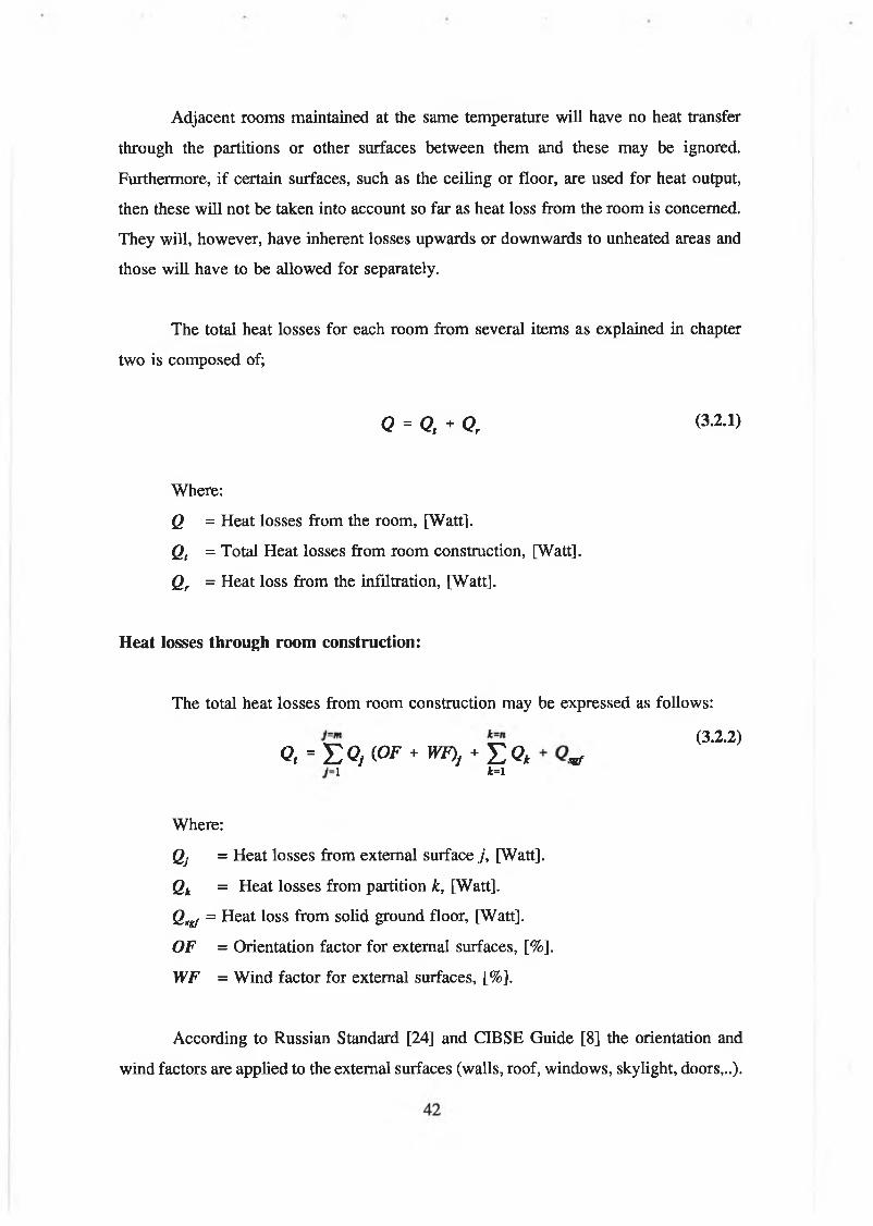
Adjacent rooms maintained at the same temperature will have no heat transfer
through the partitions or other surfaces between them and these may be ignored.
Furthermore, if certain surfaces, such as the ceiling or floor, are used for heat output,
then these will not be taken into account so far as heat loss from the room is concerned.
They will, however, have inherent losses upwards or downwards to unheated areas and
those will have to be allowed for separately.
The total heat losses for each room from several items as explained in chapter
two is composed of;
Q = Qt + Qr (3.2.1)
Where:
Q = Heat losses from the room, [Watt].
Qt = Total Heat losses from room construction, [Watt].
Qr = Heat loss from the infiltration, [Watt].
H e a t lo s s e s t h r o u g h r o o m c o n s t r u c t i o n :
The total heat losses from room construction may
<?, = E < ? y (OF *■ WF), * E < ? t 1 *=1
Where:
Qj = Heat losses from external surface j, [Watt].
Qk = Heat losses from partition k, [Watt].
Qsgf = Heat loss from solid ground floor, [Watt].
OF = Orientation factor for external surfaces, [%].
WF = Wind factor for external surfaces, [%].
According to Russian Standard [24] and CIBSE Guide [8] the orientation and
wind factors are applied to the external surfaces (walls, roof, windows, skylight, doors,..).
be expressed as follows:
(3.2.2)sgf

O r i e n t a t i o n F a c t o r : This factor may be taken from the following figure
(Fig.(3.1)) f o r all directions.
6«o
F i g . ( 3 . 1 ) Orientation Factors Diagram
W i n d F a c t o r : This factor is applied to external surfaces in the windward side
only for each place that has the orientation of the wind and the velocity. It is
selected according to these parameters. Table (3.1) shows the wind factor as
follows;
T a b l e 3 . 1 Wind Factors
Wind Factor [%]
Nature of
surface
wind Velocity [m/s]
V < 5 5 < V < 10 V > 10
Hidden 5 10 15
Exposed 10 20 30
Fig.(3.2) explains the hidden and the exposed surfaces of the buildings:
- Building No. 1 is considered as hidden if L < 5h.
- Building No. 2 is considered as a exposed.
43

Wind
F i g . ( 3 .2 ) Hidden and exposed surfaces
E x t e r n a l s u r f a c e s :
External surfaces include glass windows, glass doors, skylights, exterior walls,
exterior roof, and basement wall with U-Value calculated according to the ASHRAE
method, the heat losses from these surfaces can be calculated by the following equation:
Qj = Uj Aj ( ( , - Q ( 3 .2 .3 )
where:
Qj = Heat loss from surface j, [Watt].
Uj = Heat transfer coefficient (U-Value) of the surface j, [W/m2°C],
Aj = Area of surface j, [m2].
tj = Inside temperature in winter, [°C].
t 0 = Outside temperature in winter [°C].
I n t e r n a l s u r f a c e s ( P a r t i t i o n s ) :
These surfaces include internal walls, ceilings, floors above and below the ground, walls
below the ground and basement. The heat losses from these surfaces can be calculated
by the equation (3.2.4) as follows;
Qj - Ut A, ( r , - O ( 3 .2 .4 )
where:
tn = Next side temperature (unheated place, ground temperature, place with
44

lower temperature,....), [°C].
S o l i d g r o u n d f l o o r :
The heat loss through this surface may be calculated using the Wang and Blight
[7] equation and equation (3.2.1) where the U-Value has to be calculated by the
Billington Eq. (3.6.4) given by [8,17] and the bigger value is taken. Wang and Blight
relationship is written as follows;
( 3 .2 .5 )Q«f = Fi P ft - o
Where:
Q sgf = Heat loss from solid ground floor, [Watt],
F2 = Heat loss coefficient, per metre of perimeter, Table 5 chapter 26 in the
ASHRAE Fundamentals [7], [W/°C.m].
P = Perimeter or exposed edges of floor, [m].
I n f i l t r a t i o n h e a t l o s s :
Infiltration of outside air causes both sensible and latent heat loss. The energy
required to raise the temperature of outdoor infiltration air to indoor air temperature is
the sensible component. The heat loss associated with the net loss of moisture from the
space is classified as the latent component.
S e n s i b l e H e a t l o s s :
The energy required to warm outdoor air entering by infiltration to the
temperature of the room is given by:
^ v p ft - 0 (3.2.6)
45

Where:
qa = Sensible heat loss, [W].
Cp = Specific heat of air, [J/kg°C].
v = Flow rate of outdoor air entering building, [L/s].
p = Density of air at temperature t0, [kg/m3].
using standard air where p = 1.2 Kg/m3, and Cp = 1.0 Kj/Kg°C, Equation (3.2.7)
reduces to:
qs = 1.2 v ( f 4 - t^ ( 3 . 2 . 7 )
The flow rate of outdoor air entering depends on wind speed, direction, width
of cracks, size of openings, type of openings and other factors. There are two
methods used to obtain the quantity of infiltration air rate which is explained as
follows:
© C r a c k l e n g t h m e t h o d :
For the designer who prefers the crack method, the basis of calculation is the
amount of crack used for computing the infiltration heat loss which should not
be less then half the total length of the crack in the outside walls of the room.
In buildings without partitions, air entering through cracks on the windward side
must leave through cracks on the leeward side. Therefore, one-half of the total
crack for each side and end of the building is used for calculation. In a room
with one exposed wall, all the crack is used. With two, three, or four exposed
walls, the wall with the crack that will result in the greatest or least air leakage,
half the total crack is used, whichever is greater.
In a residence, total infiltration loss of the house is generally considered equal
to the sum of infiltration losses of the various rooms. But, at any given time,
infiltration takes place only on the windward side or sides and not on the
leeward. Therefore, for determining total heat requirements of larger buildings,
46

it is more accurate to base total infiltration loss on the wall with the most total
crack or at least half the total crack in the building, whichever is greater.
When the crack method is used for estimating leakage, the air flow rate may
be calculated from equation (3.2.8) [16] as follows:
l> - C , ¿ ( A p ) " / , / 2 ( 3 -2 -8 )
where:
Ci = Window infiltration coefficient for pressure difference of 1 Pa, [L/s m].
L = Length of window or door crack to be considered, [m].
Ap = Applied pressure difference, [Pa].
n = Exponent relating volume flow rate to applied pressure difference
generally lies in the range 0.6 to 0.7, for Ireland is taken 0.63 [20],
f l = Correction factor for geographical location, Table (3.2).
f 2 = Correction factor for internal resistance, Table (3.3).
T a b l e ( 3 .2 ) Correction factor for geographical location
W i n d s p e e d e x c e e d e d f o r 5 0 %
o f t i m e , [ m / s ]
C o r r e c t i o n f a c t o r , f x
s h e l t e r e dl o c a t i o n( i n l a n d )
E x p o s e dl o c a t i o n( c o a s t a l )
3.5 0.85 0.79
4.0 1.0 0.94
4.5 1.16 1.09
5.0 1.32 1.25
5.5 1.49 1.40
6.0 1.67 1.57
6.5 1.84 1.73
47

Table (3.3) Correction factor for internal resistance.
W i n d o w t y p e I n t e r n a l s t r u c t u r eC o r r e c t i o n
f a c t o r , f 2
All Types Single plan (no full partitioning 1.0
Short length of well fitting window opening joint (say, 20% of facade openable)
single corridor with many side doors: liberal internal partitioning with few interconnecting doors
1.0
long length of well fitting window or short length of poor fitting window joint (say, 20% to 40% of facade openable)
Single corridor 1.0
Liberal partitioning 0.8
Long length of poor fitting window joint (say, 40% to 50% of facade openable)
Single corridor 0.8
Liberal partitioning 0.65
Very long length of poor fitting window joint (say, >50% of facade openable)
Single corridor 0.65
Liberal partitioning 0.4
The infiltration coefficient C, is defined as the volume flow rate of air per unit
length of the opening at an applied pressure difference of 1 Pa, the values of the
infiltration coefficient C, being shown in Table (3.2) . The applied pressure
difference may be defined as follows:
A p = i Cp p u* ( 3 .2 .9 )2
where:
Cp = Pressure coefficient
u = Mean wind speed at height equal to building height, [m/s]
48

Table (3.4) Air infiltration through windows, [8].
W i n d o w t y p e
w i n d o w i n f i l t r a t i o nc o e f f i c i e n t f o r p r e s s u r e
d i f f e r e n c e o f 1 P a C i [ I i t t e r / s m ]
Horizontally or vertically pivoted weather stripped 0.05
Horizontally or vertically pivoted non-weather stripped 0.25
Horizontally or vertically sliding weather stripped 0.125
Horizontally or vertically sliding non-weather stripped 0.25
Wind speed varies with height and location. Equation (3.2.10) gives an
expression which relates this variation to the nature of the terrain across which
the wind is passing:
u — u K Z° (3.2.10)m S
where:
u m = Mean wind speed at 10 m height in open country (design wind speed of
each place) , [m/s]
Z = Height above ground, [m]
Parameter relating wind speed to nature of terrain
a = Exponent relating wind speed to height above ground
Table (3.5) gives the values of the coefficients Ks according to four types of
terrain as follows:
Table (3.5) Values o f parameters Ks and a.
T e r r a i n K , a
Open flat country 0 .6 8 0 . 1 7
Country with scattered windbreaks 0 .5 2 0 .2 0
Urban 0 .3 5 0 .2 5
City 0 . 2 1 0 .3 3
4 9
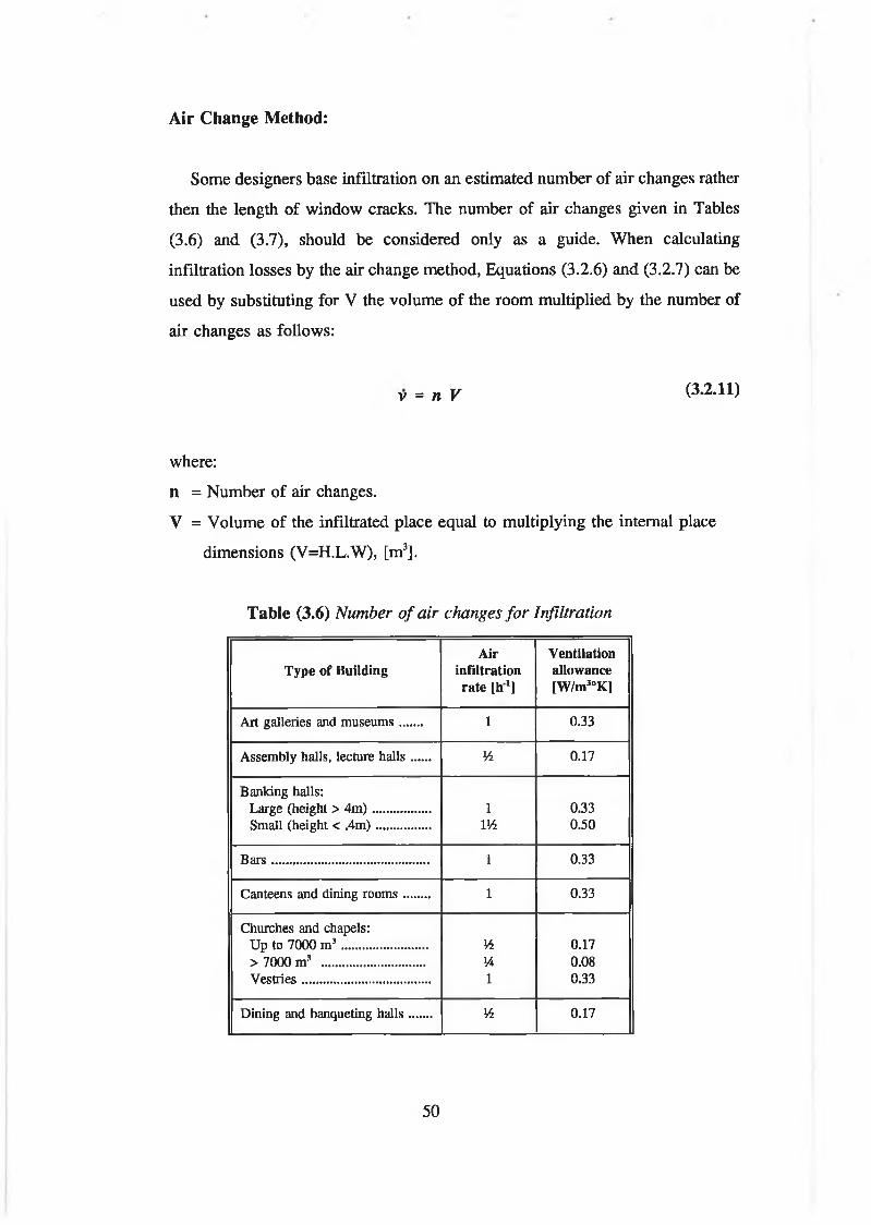
Air Change Method:
Some designers base infiltration on an estimated number of air changes rather
then the length of window cracks. The number of air changes given in Tables
(3.6) and (3.7), should be considered only as a guide. When calculating
infiltration losses by the air change method, Equations (3.2.6) and (3.2.7) can be
used by substituting for V the volume of the room multiplied by the number of
air changes as follows:
v = n V (3.2.11)
where:
n = Number of air changes.
V = Volume of the infiltrated place equal to multiplying the internal place
dimensions (V=H.L.W), [m3].
Table (3.6) Number o f air changes fo r Infiltration
Type of BuildingAir
infiltration rate [h 1]
Ventilationallowance[W/m3oK]
Art galleries and museums.. 1 0.33
Assembly halls, lecture halls.. Vi 0.17
Banking halls:Large (height > 4m)....... 1 0.33Small (height < .4m)....... VA 0.50
Bars.................... 1 0.33
Canteens and dining rooms... 1 0.33
Churches and chapels:Up to 7000 m 3 ........... V* 0.17> 7000 m 3 ............. V4 0.08Vestries................ 1 0.33
Dining and banqueting halls.. Vi 0.17
50
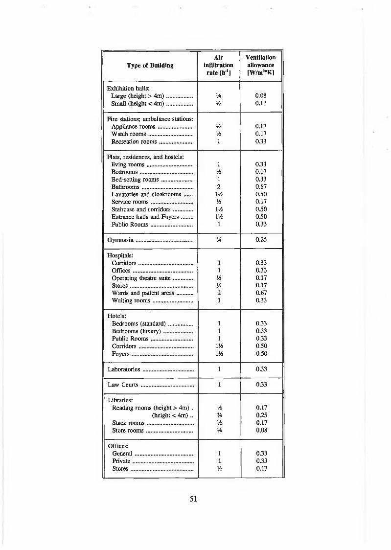
Air VentilationType of Building infiltration allowance
rate [h'1] [W/m3oK]
Exhibition halls:Large (height > 4m)....... ]/4 0.08Small (height < 4m)....... Vi 0.17
Fire stations: ambulance stations:Appliance rooms......... Vi 0.17Watch T o o m s ............... Vi 0.17Recreation rooms......... 1 0.33
Flats, residences, and hostels:living rooms............ 1 0.33Bedrooms............... Vi 0.17Bed-setting rooms........ 1 0.33Bathrooms.............. 2 0.67Lavatories and cloakrooms.. ivi 0.50Service rooms........... Vi 0.17Staircase and corridors..... lVi 0.50Entrance halls and Foyers... lVi 0.50Public Rooms........... 1 0.33
Gymnasia............... % 0.25
Hospitals:Corridors............... 1 0.33Offices................ 1 0.33Operating theatre suite..... Vi 0.17Stores ................. Vi 0.17Wards and patient areas.... 2 0.67Waiting rooms........... 1 0.33
Hotels:Bedrooms (standard)...... 1 0.33Bedrooms (luxury)........ 1 0.33Public Rooms........... 1 0.33Corridors............... lVi 0.50Foyers................. lVi 0.50
Laboratories.............. 1 0.33
Law Courts............... 1 0.33
Libraries:Reading rooms (height > 4m) . Vi 0.17
(height < 4m) .. 3/4 0.25Stack rooms............. Vi 0.17Store rooms............. V4 0.08
Offices:General................ 1 0.33Private................ 1 0.33Stores ................. Vi 0.17
51

Air VentilationType of Building infiltration allowance
rate [h 1] [W/m3oK]
Police Stations:Cells.................. 5 1.65
Restaurants and tea shops.... 1 0.33
Schools and colleges:Classrooms............. 2 0.67Lecture rooms........... 1 0.33Studios................ 1 0.33
Shops and showrooms:Small.. ............... 1 0.33Large.................. Vi 0.17Department store......... V* 0.08fitting rooms............ m 0.50Store rooms............. Vi 0.17
Sports pavilions:Dressing rooms........... i 0.33
Swimming baths;Changing rooms.......... a 0.17Bath hall............... Vi 0.17
Warehouses:Working and packing spaces ... Vi 0.17Storage spaces ........... V* 0.08
Table (3.7) Number o f air changes fo r Infiltration
ConstructionAir
infiltration rate [h'1]
Ventilationallowance[W/m3oK]
Multi-storey, brick or concrete construction: Lower and intermediate floors...... 1 0.33Top floor with flat roof...... 1 0.33Top floor with sheeted roof, lined VA 0.42Top floor with sheeted roof, lined lVi 0.50
Single-storey unpartitioned spaces: Brick or concrete construction Up to 300 m 3 .......... lVi 0.50300 to 3000 m 3 ............. 3/4 0.25300 to 10000 m 3 ............. Vi 0.17Over 10000 m 3 ............. V4 0.08
52
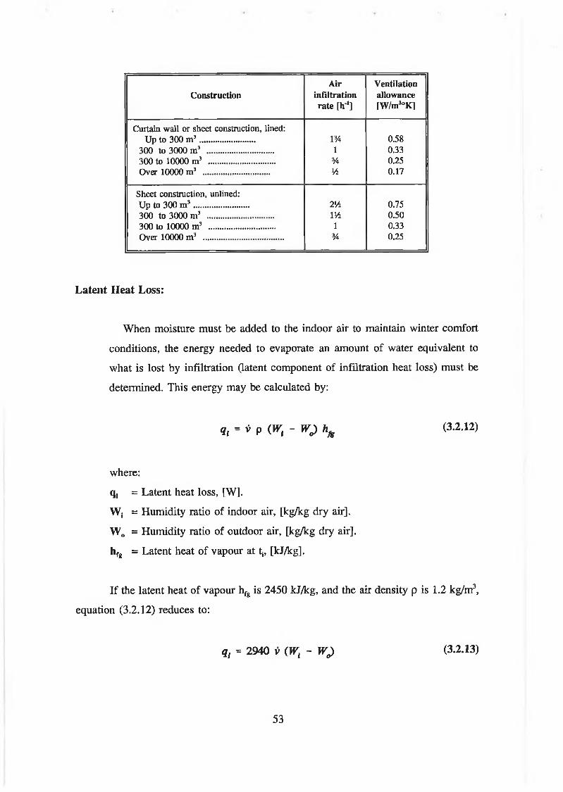
Air VentilationConstruction infiltration allowance
rate [h l] [W/m3oK]
Curtain wall or sheet construction, lined:Up to 300 m 3 .......... 1% 0.58
300 to 3000 m 3 ............. 1 0.33300 to 10000 m 3 ............. % 0.25Over 10000 m 3 ............. Vi 0.17
Sheet construction, unlined:Up to 300 m 3 ........... 2Vi 0.75300 to 3000 m 3 ............. lVi 0.50300 to 10000 m 3 ............. 1 0.33Over 10000 m 3 ............... % 0.25
L a t e n t H e a t L o s s :
When moisture must be added to the indoor air to maintain winter comfort
conditions, the energy needed to evaporate an amount of water equivalent to
what is lost by infiltration (latent component of infiltration heat loss) must be
determined. This energy may be calculated by:
q, = * p (W, - w y hk ( 3 . 2 . 1 2 )
where:
q , = Latent heat loss, [W].
Wj = Humidity ratio of indoor air, [kg/kg dry air].
W 0 = Humidity ratio of outdoor air, [kg/kg dry air].
h fg = Latent heat of vapour at tj, [kJ/kg].
If the latent heat of vapour hfg is 2450 kJ/kg, and the air density p is 1.2 kg/m3,
equation (3.2.12) reduces to:
q, = 2940 v (Wt - W J (3.2.13)
53

3.2.2 H e a t i n g p r o g r a m e x e c u t i o n p r o c e d u r e s :
Fig.(3.3) and Fig.(3.4) show the procedures of the heating load calculation. The
execution of the heating program through selecting " H e a t i n g " command from the
" P r o g r a m s " pull-down menu takes the user through a menu for selecting the heating
load calculation method, which are " R o o m B y R o o m " and " W h o l e B u i l d i n g " . When
the user selects " R o o m B y R o o m " option the program will go through a procedure that
enters the information for each space then calculate the heating load for the room space
and so on for all rooms in the building. If the user selects the " W h o l e B u i l d i n g " option
the program will go through the procedure that enter the input data information for all
spaces then the calculation for the heating loads for the whole building takes place. For
that a menu is displayed on the screen for the selection as following:
This program calculates the Heating Load for
Commercial and Scientific Buildings Would you like to calculate:
1 -
2 - Whole Building
After that an entry input data for the building are displayed to input the building
information which contains building description, dimensions, total area, number of
storeys, three storeys that may be multiple in the building and the infiltration input data
which may be computed by crack method (glazing sides, windows types, building
exposure and building internal layout). The entry input data menu, which is displayed
automatically by pressing the " E n t e r " key on the keyboard after selecting the type of
procedures. The input data is requested via a menu screen that is accessed through the
last menu. The entry data menu screens contain descriptive titles before each input field
or data area. The descriptive titles for input fields will appear in reverse video on the
monitor. To enter data, the user has to position the cursor to an input field and type in
the desired value. Any input data field can always be edited for modification or
correction. This entry data menu for the building can be displayed on the screen as
54

55

ST A R T
Fig. (3.4) Flow Diagram o f The Heating Load Calculation Steps
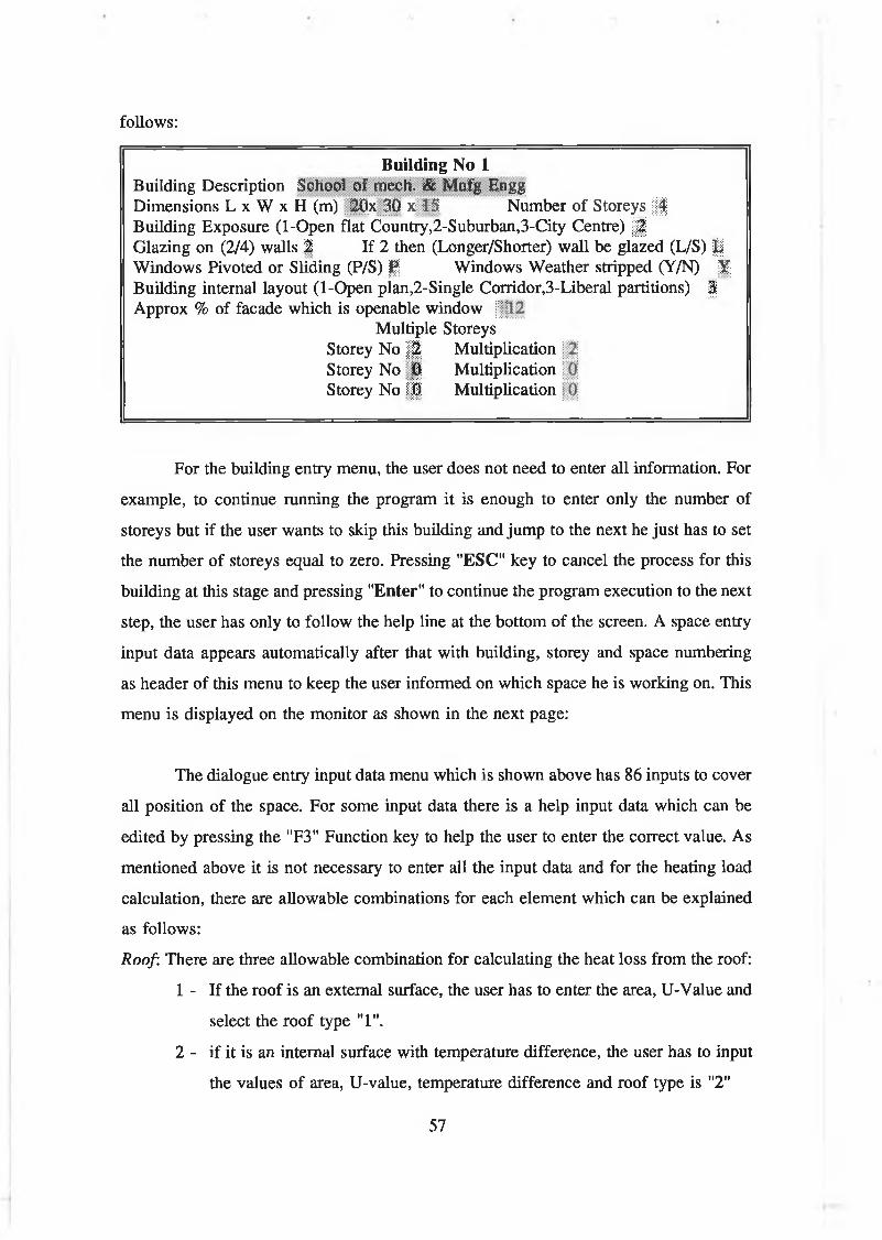
follows:
B u i l d i n g N o 1Building Description School of tnech. & Mnfg EnggDimensions L x W x H (m) 20x 30 x 15 Number of Storeys §§Building Exposure (1-Open flat Country,2-Suburban,3-City Centre) ¡1 Glazing on (2/4) walls I If 2 then (Longer/Shorter) wall be glazed (L/S) §| Windows Pivoted or Sliding (P/S) ff Windows Weather stripped (Y/N) X Building internal layout (1-Open plan,2-Single Corridor,3-Liberal partitions) § Approx % of facade which is openable window
Multiple StoreysStorey No j | | Storey No 0 Storey No i f f
MultiplicationMultiplicationMultiplication
For the building entry menu, the user does not need to enter all information. For
example, to continue running the program it is enough to enter only the number of
storeys but if the user wants to skip this building and jump to the next he just has to set
the number of storeys equal to zero. Pressing " E S C " key to cancel the process for this
building at this stage and pressing " E n t e r " to continue the program execution to the next
step, the user has only to follow the help line at the bottom of the screen. A space entry
input data appears automatically after that with building, storey and space numbering
as header of this menu to keep the user informed on which space he is working on. This
menu is displayed on the monitor as shown in the next page:
The dialogue entry input data menu which is shown above has 86 inputs to cover
all position of the space. For some input data there is a help input data which can be
edited by pressing the "F3" Function key to help the user to enter the correct value. As
mentioned above it is not necessary to enter all the input data and for the heating load
calculation, there are allowable combinations for each element which can be explained
as follows:
Roof. There are three allowable combination for calculating the heat loss from the roof:
1 - If the roof is an external surface, the user has to enter the area, U-Value and
select the roof type "1".
2 - if it is an internal surface with temperature difference, the user has to input
the values of area, U-value, temperature difference and roof type is "2"
57

B u i l d i n g N o . 1 S t o r e y N o . 1 S p a c e N o . 2Dimension LxWxH 5.6x6.3x2 7 Description N30 ; Printer Room Dry Bulb Temperature tdb 21,0 °C Relative Humidity 50 %
Roof InformationRoof Area (m2) :) .0,00 U-Value (W/m2oC) 0.000 Suspended (Y/N) I SkyLight Area 0.00 SkyLight U-Value 0.000 Temp. Diff Ipp
Walls InformationWall No. 1 2 3 4 5 6 7 8W1 Orientations SW SW NEW1 Area (m2) É I® 3.47 15.12 0.00 0.00 0.00 0.00 0.00W1 U-Value 0:481 0.973 1.295 0 0 0.0 0.0 0.000 0 000W1 (1-Ex,2-In,3-Bs) 1 § 1 i ....1 1 1Gl Area 6.94 0.00 0.00 000 0.00 0.00 0.00 Ü ÉGl U-Value 3,200. 0.000 0.000 0.000 0.000 0.000 0.000 0.000Wind & Orien. Factor | | 0 10 o 0 ' i l l 0 10 :QPartition Temp. Diff 0.0 0.0 3.0 0.0 fp .o 0.0 0.0 0.0
Floor InformationArea (m2) i | | l | | U-Value(W/m2oC) 0 330 Temp. Diff i l l
Type (1 -Inter,2-Solid Gmd.,3-Bs) §Infiltration (1-Air Changes,2-Crack) | Air Changes No. 1.5 Crack Lngth 0.0 Ventilation (1-Air Chngs,2-CFM/Person) | Air Chngs No 0,0 CFM/Person 0.0
3 - if it is an internal surface without temperature difference, the user has to set
the values equal to zero.
Wall: There are four allowable combinations for calculating the heat loss from the wall:
1 - If the wall is an external surface, the user has to enter the area, U-Value,
glass area, glass U-value, wind and orientation factor and select the wall
type "1".
2 - if it is a partition with temperature difference, the user has to input the
values of area, U-value, temperature difference and wall type is "2"
3 - if it is a partition without temperature difference, the user has to set the
values equal to zero.
4 - if it is a basement , the user has to enter the values of U-value, depth of
basement in glass area input, length of basement in glass U-value input and
wall type is "3"
Floor. For this item also, there are three allowable combinations:
1 - If the floor is an internal surface, the user has to enter the area, U-Value,
temperature difference, and select the floor type "1".
58

2 - if it is a solid ground surface, the user has to enter the values of area, U-
value, space-ground temperature difference and floor type is "2"
3 - if it is an internal surface without temperature difference, the user has to set
the values equal to zero.
4 - if it is a basement, the user has to enter the values of U-value, depth of
basement in glass area input and wall type is "3"
Infiltration: The heat loss from infiltration can be calculated using two methods (for the
calculation the flow rate of the air) as mentioned before, then the user has to select the
type of infiltration, "1" for air change method and if it is selected the user also has to
enter number of air changes, or "2" for crack method and if selected the user has to
enter the crack length. Fig.(3.5) shows the procedure for calculating the heat loss
through infiltration.
Ventilation: If the ventilation load is needed and if there is no need to design a separate
system for ventilation, then the heating load is included as the heat loss from ventilation.
The user has to enter the ventilation information if ventilation is needed, e.g. type of
ventilation, "1" for air change method and if it is selected the user also has to enter
number of air changes, or "2" for CFM per person method and if it is selected the user
has to enter the CFM per person. Fig.(3.6) shows the procedure of calculating the heat
loss through ventilation.
Some of the input data are "help" input data, which are asked for by pressing
"F3" function key after moving the cursor to that input. Some of these input data are:
* U-Values for all structures (roofs, walls, floors, glass, sky lights).
* Wind and orientation factors.
* Air changes for infiltration.
* Air changes for ventilation.
* CFM per person for ventilation.
59

On window type select Ci from Table(3.4)
On wind speed select fl from Table(3.2)
Crack — Infiltrationcalculation method
Air Changes
On window facade openable select f2 from Table(3.3)
Calculate the flow rate using Eq.(3.2.11)
on Terrain select Ks & a from Table(3.5)
Calculate the mean wind speed using Eq.(3.2.10)
Calculate the pressure difference using Eq.(3.2.9)
Calculate the flow rate using Eq.(3.2.8)
Calculate sensible & latent heat gain from infiltration using Eq.(3.2.7)&Eq.(3.2.13)
respectively
C e n d s u b )
Fig. (3.5) Flow diagram o f the infiltration load calculation steps
Fig. (3.6) Flow diagram o f the ventilation load calculation steps
60

3.3 VENTILATION PROGRAM:
When positive ventilation using outdoor air is provided by an air heating or air
conditioning unit, the energy required to warm the outdoor air to the space temperature
must be provided by the unit. The principle for calculation of this load components is
identical to that for infiltration. If mechanical exhaust from the space is provided in an
amount equal to the outdoor air drawn in by the unit, the unit must also provide for
natural infiltration losses.
The amount of ventilation required in any situation depends on the type of
building, the number of people and the use being made of the space. Ventilation must
comply with local regulations and the provisions of the health and safety at work act,but
the ASHRAE [7], CIBSE [8], for example sets out model recommendations which can
be used in the absence of more specific requirements. Ventilation rates can be expressed
in two ways:
* As a number of complete air changes (the most commonly used method).
* or by a given amount of fresh air per person occupying the space.
Air changes must be of outside or fresh air, changing air by recirculation only will not
remove or dilute contaminants.
The recommended rates [7,8] take into account of the occupancy levels and
activity for specific locations. In some situations such as animal and chemical
laboratories, workshops, kitchens, ...etc, where the activity itself is the greatest
contributor to the need for ventilation, the rate is usually expressed as a number of air
changes, not as fresh air per person. To improve the air quality and further dilute the
concentration of contaminants, these ventilation rates can be increased. However, the
ventilation rate, the air direction and movement must be controlled. Unless some form
of heat recovery is used, the need for heating or cooling due to the increase in the
ventilation rate will increase the building’s energy consumption.
3.3.1 V e n t i l a t i o n p r o g r a m f o r m u l a t i o n :
61

The same formulas (Eq.(3.2.7) and Eq.(3.2.13)) for the infiltration used in the
heating program can be used here but only the quantity of the flow rate is different. As
explained above there are two methods to determine the quantity of ventilation:
* By knowing the number of persons and the usage of the place, the flow rate
can be defined by multiplying the number of persons by the CFM (Cubic Feet
per Minute) per person as follows:
v = 1700 n CFM i3 -3 -1)
where:
v = Flow rate of outdoor air entering building, [L/s].
n = Number of persons.
CFM = Cubic feet per minute per person, [ftVmin].
* Or by knowing the number of air changes per cubic meter of the place
according to its applications, then Eq.(3.2.11) can be used for this option.
3 .3 .2 V e n t il a t io n p r o g r a m e x e c u t io n p r o c e d u r e s :
Combination of Fig.(3.3) and Fig.(3.6) shows the execution steps for the
ventilation load calculation. The execution of the ventilation programme through
selecting " V e n t i l a t i o n " commands from the " P r o g r a m s " pull-down menu takes the user
through a menu to give the user a choice to calculate the ventilation loads of the
building room by room or for the whole building as explained in the heating
programme. A menu is displayed on the screen for the selection as following:
This program calculates the Ventilation Load for
Commercial and Scientific Buildings Would you like to calculate:
1 - Room By Room2 - Whole Building
After selecting the calculation method, an entry input data menu for the building
is displayed as following:
62
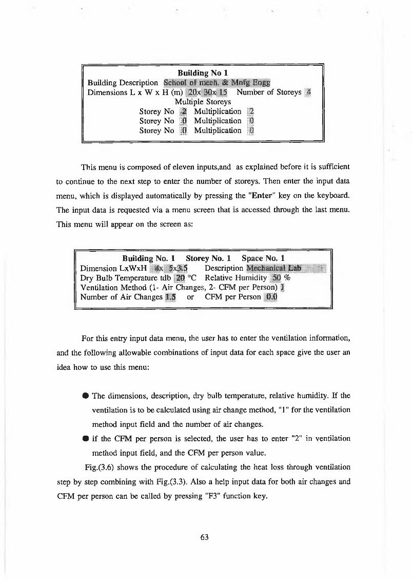
B u i l d i n g N o 1Building Description School of mech. & Mnfg Engg Dimensions L x W x H (m) 2Qx 30x15 Number of Storeys 4
Multiple Storeys Storey No g|| Multiplication ¡§j Storey No §j§ Multiplication ¡¡§Storey No p Multiplication |§
This menu is composed of eleven inputs,and as explained before it is sufficient
to continue to the next step to enter the number of storeys. Then enter the input data
menu, which is displayed automatically by pressing the " E n t e r " key on the keyboard.
The input data is requested via a menu screen that is accessed through the last menu.
This menu will appear on the screen as:
B u i l d i n g N o . 1 S t o r e y N o . 1 S p a c e N o . 1Dimension LxWxH 4x 5x3.5 Description Mechanical Lab Dry Bulb Temperature tdb 20 °C Relative Humidity 100 % Ventilation Method (1- Air Changes, 2- CFM per Person) § Number of Air Changes 1.5 or CFM per Person 0,0
For this entry input data menu, the user has to enter the ventilation information,
and the following allowable combinations of input data for each space give the user an
idea how to use this menu:
• The dimensions, description, dry bulb temperature, relative humidity. If the
ventilation is to be calculated using air change method, "1" for the ventilation
method input field and the number of air changes.
• if the CFM per person is selected, the user has to enter "2" in ventilation
method input field, and the CFM per person value.
Fig.(3.6) shows the procedure of calculating the heat loss through ventilation
step by step combining with Fig.(3.3). Also a help input data for both air changes and
CFM per person can be called by pressing "F3" function key.
63
3 .4 C O O L I N G L O A D P R O G R A M :
The variables affecting cooling load calculations are numerous, often difficult to
define precisely, and always intricately inter-related. Many cooling load components
vary widely in magnitude during a 24 hour period. Since these cyclic changes are often
out of phase with each other, they must be analyzed to establish the maximum cooling
load for a building or zone. A zoned system need recognize no greater total cooling load
capacity than the largest hourly summary of simultaneous zone loads throughout a
design day; but it must handle the peak cooling load for each zone at its peak hour. At
certain times of the day during the heating or intermediate seasons, some zones may
require heating while others require cooling.
A proper cooling load calculation gives values adequate for proper performance.
Variation in the heat transmission coefficients of typical building materials and
composite assemblies, the differing motivations and skills of those who construct the
building, and the manner in which the building is operated are some of the variables that
make a numerically precise calculation impossible. While the designer uses reasonable
measures to include these factors, the calculation is still only a good estimate of the
actual cooling load. The calculation of space sensible and cooling loads is a key step in
any building energy estimations. There are two widely used methods for doing these
calculations:
1) The heat balance method.
2) The weighting factor method.
The heat balance method for calculating net space sensible loads is the more
fundamental of the two methods. Its development relies on the first law of
thermodynamics (conservation of energy) and the principles of matrix algebra. Since
there are fewer assumptions required than for the weighting factor method, it is also the
more flexible of the two. However, the heat balance method requires more calculations
at each point in the estimation process, and therefore is more costly in terms of
computer resources.
64
I

The purpose of the heat balance method is to allow calculation of the net sensible
heating and cooling load on the space air mass. The approach is to write a heat balance
equation for each enclosing surface, and for the room air. This set of equations take
account of the conduction, convection and radiation heat exchange between the room air,
surrounding surfaces, infiltration and internal energy sources. They are then solved for
the unknown surface and air temperatures. Once these temperatures are known, they can
be used to calculate the convective heat flow to or from the space air mass. The latter
constitutes the heating or cooling load which must be met by the space conditioning
equipment, CLTD/CLF method in ASHRAE 1989 Fundamentals Handbook simulates
this method which has been taken for the calculation of cooling loads.
The weighting factor method of calculating spaces sensible load, first introduced
by Mitalas and Stephenson [25-27], is a simple but flexible technique that accounts for
the important parameters affecting building energy flow. It represents a compromise
between simpler method, such as steady-state calculation that ignores the ability of the
building mass to store energy, and more complex methods, such as complete energy
balance calculations. With this method, space heat gains at constant space temperature
are determined from the building architectural data, the ambient weather conditions and
internal load profiles. These space heat gain are used, along with the characteristics and
availability of heating and cooling systems for the building, to calculate air temperatures
and heat extraction rates.
The weighting factor method is based on the assumption that the heat transfer
processes occurring in a room can be described by linear equations; and thus the
superposition principle can be used for calculation of cooling load and space
temperature. Two sets of weighting factors are used: heat gain and air temperature. Heat
gain weighting factors represent transfer functions which relate space cooling load to
instantaneous heat gain. Air temperature weighting factors represent transfer functions
that relates room air temperature to the net energy load of the room.
In the weighting factor method, a two-step process is used to determine the air
temperature and heat extraction rate of a room or building zone for a given set of
65
I

conditions:
* In the first step, the room’s air temperature is assumed to be fixed at some
reference value. This reference temperature is usually chosen to be the average
air temperature expected for the room over the day period. Instantaneous heat
gain is calculated on the basis of this constant air temperature. A space sensible
cooling load for the room, defined as the rate at which energy must be removed
from the room to maintain the air temperature fixed at its reference value, is
calculated on the basis of this constant air temperature. A space sensible cooling
load for the room, defined as the rate at which energy must be removed from the
room to maintain the air temperature fixed at its reference value, is calculated
for each type of instantaneous heat gain. The cooling load generally differs from
the instantaneous heat gain because some of the energy from heat gain can be
absorbed by walls or furniture and stored for later release to the air. At the end
of the first step, the cooling load from the various heat gains are summed to give
a total cooling load for the room.
* In the second step, the total cooling load is used (along with information on
the HVAC system relevant to the room and a set of air temperature weighting
factors) to calculate the actual heat extraction rate and air temperature. The
actual heat extraction rate differs from the cooling load because, in practice, the
air temperature can vary from the reference value used to calculate the cooling
load or because of the HVAC system characteristics.
3.4.1 C ooling p r o g r a m theoretical analyses:
To calculate a space cooling load using the CLTD/CLF convention, one has to
follow the procedure for the basic heat gain calculations of solar radiation, total heat
gain through exterior wall and roof, heat gain through the interior surfaces, and heat gain
through infiltration and ventilation. Then the total heat gain or the cooling load for each
room from several items as explained above is composed of;
Q t o * , = <?,+<?, (3A1)
66

Where:
(¿Total = Total heat gain from the room, [Watt].
Qs = Total sensible heat gain from the room, [Watt].
Q, = Total latent Heat gain from the room, [Watt].
Total sensible heat gain:
The total sensible heat gain from the room may be expressed as follows:
/=7 ft=8 l = n
Q = Q sroof + Q swall(2j + l) + ] C (Q sg laa + Q cglas^Ç lk + l) + E Q pa j= \ *=1 /=1
+ Q speoplt + Q lig h t + Q Power + Qsappüanc* + QSii\flltrotion + Q s
?Partition +
Sventilation
(3.3.2)
Where:
Qsroor
Qswall
QsglassQcglass
Qpartilion
Qspeople
QLightQpower
Qsappliance
Qsinfiltration
Qsventilation
= Solar heat gain from the roof, [Watt]
= Solar heat gain from the wall, [Watt]
= Solar heat gain from the glass, [Watt]
= Conduction heat gain from the glass, [Watt]
= Heat gain from partition, [Watt].
= Sensible heat gain from people, [Watt].
= Heat gain from Lights, [Watt].
= Heat Gain form motors, [Watt].
: Sensible heat gain from appliances, [Watt].
= Sensible heat gain from infiltration, [Watt].
= Sensible heat gain from ventilation, [Watt].
Total latent heat gain:
The total latent heat gain from the room may be expressed as follows:
— Q.Lptoplt + Q¿appliance + QuqfiltnUlon + Q * ¿ventilation(3 .3 .3)
67

Where:
Qi peopie = Latent heat gain from people, [Watt].
QLappiiance = Latent heat gain from appliances, [Watt].
Qurifiitration = Latent heat gain from infiltration, [Watt].
QLventiiation = Latent heat gain from ventilation, [Watt].
Solar Heat Gains:
The heat gain from solar radiation through the external surfaces can be
determined as following:
Roof:
< ?W = CLTDccrr (3.3.4)
where:
Ur0of = U-Value for the roof, [Watt/m2oC]
Aroof = Roof area, [m2]
CLTDcorr = the correction of Cooling Load Temperature Difference, [°C]
The CLTDcori for roof can be expressed as follow;
CLIDcorr = \.(CLTD + LM) K + (25.5-r*) + (to - 29.4)] / (3.3.5)
where:
CLTD = Cooling Load Temperature Difference for roof Table 29 chapter 26
at ASHRAE Fundamental 1989, [°C]
LM = CLTDcoit for Latitude and Month applied to Walls and Roofs.
K = Color adjustment factor and is applied after first making month-
latitude adjustment:
K = 1.0 if dark coloured or light in an industrial area.
K = 0.5 if permanently light-coloured (rural area).
68

Wall:
25.5,29.4 = Constants
tR = Room temperature, [°C].
ta = The average outside temperature, [°C].
f = Factor for attic fan or ducts above ceiling applied after all other
adjustments have been made:
/ = 1.0 no attic or ducts.
/ = 0.75 positive ventilation
where:
Uwaji = U-Value for the wall, [Watt/m2oC]
Awa,| = wall area, [m2]
CLTDcon. = the correction of Cooling Load Temperature Difference, [°C]
The CLTDcon. for walls can be expressed as follow;
c LTDcorr = (CLTD + LM) K + (25.5-i*) + (ta - 29.4) (3.3.7)
where:
CLTD = Cooling Load Temperature Difference for wall Table 31 chapter 26
at ASHRAE Fundamental 1989, [°C].
K = Color adjustment factor and is applied after first making month-latitude
adjustment:
K = 1.0 if dark coloured or light in an industrial area.
K = 0.83 if permanently medium-coloured (rural area).
K = 0.65 if permanently light-coloured (rural area).
Glass and Sky light:
The basic equation for evaluating heat gain from transmitted and absorbed solar
69
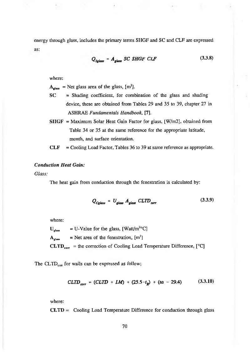
energy through glass, includes the primary terms SHGF and SC and CLF are expressed
- AlUa SC SHGF CLF (3-3-8)
where:
Agi^ = Net glass area of the glass, [m2].
SC = Shading coefficient, for combination of the glass and shading
device, these are obtained from Tables 29 and 35 to 39, chapter 27 in
ASHRAE Fundamentals Handbook, [7].
SHGF = Maximum Solar Heat Gain Factor for glass, [W/m2], obtained from
Table 34 or 35 at the same reference for the appropriate latitude,
month, and surface orientation.
CLF = Cooling Load Factor, Tables 36 to 39 at same reference as appropriate.
Conduction Heat Gain:
Glass:
The heat gain from conduction through the fenestration is calculated by:
<?<*.» - «.to V . C L T D ™ (3-3-9>
where:
Ugiass = U-Value for the glass, [Watt/m2oC]
Agi^ = Net area of the fenestration, [m2]
CLTDcorT = the correction of Cooling Load Temperature Difference, [°C]
The CLTDcorr for walls can be expressed as follow;
C L I D corr = {CLTD + LM) + (25.5-ts) + (ta - 29.4) (3.3.10)
where:
CLTD = Cooling Load Temperature Difference for conduction through glass
70

Table 33 chapter 26 at ASHRAE 1989 Fundamentals Handbook,
[°C].
Partitions, Ceilings, Floors:
The heat gain form these surface can be calculated by:
Where:
U = Design heat transfer coefficients, [W/m2 °C].
A = Areas calculated from building plans, [m2].
At = Design temperature difference, unconditioned area to room, [°C].
Internal:
People:
The heat gain from the people is composed of two components as :
Sensible Heat gain: it can be calculated by:
< W - N (3.3.12)
Where:
N = Number of people.
PHGSensible = Sensible heat gain from occupant, [W/Person].
Latent Heat gain: it can be calculated by:
< W - N p h g l ~ * (3 -3 -13)
Where:
Qi.peopie = Latent heat gain from people, [Watt],
PHGLatent = Latent heat gain from occupant, [W/Person].
Lights:
The heat gain from light can be calculated by the following expression:
= A LHG (3.3.14)
71
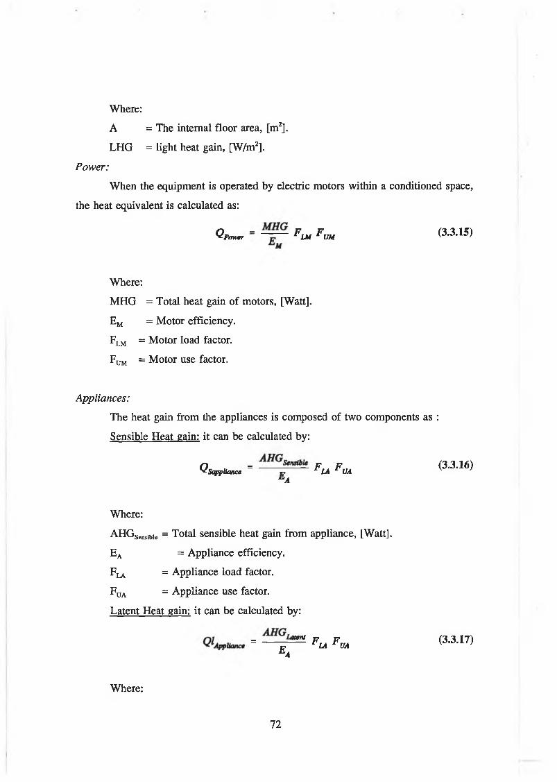
Where:
A = The internal floor area, [m2].
LHG = light heat gain, [W/m2].
Power:
When the equipment is operated by electric motors within a conditioned space,
the heat equivalent is calculated as:
Q p t r w r ~ ^ I M F U M (3.3.15)
Where:
MHG = Total heat gain of motors, [Watt].
Em = Motor efficiency.
Flm = Motor load factor.
Fum = Motor use factor.
Appliances:
The heat gain from the appliances is composed of two components as :
Sensible Heat gain: it can be calculated by:
O = F A F (3.3.16)V Sapptiance r . LA UA" A
Where:
AHGSensible = Total sensible heat gain from appliance, [Watt].
Ea = Appliance efficiency.
Fla = Appliance load factor.
Fua = Appliance use factor.
Latent Heat gain: it can be calculated by:
- — ¡r5 * f m f m (3-3-17)" A
Where:
72

QUppiiance = Latent heat gain from appliances, [Watt].
AHG^ent = Total latent heat gain from appliance, [Watt].
Infiltration and Ventilation:
Infiltration or Ventilation heat gains are also composed of sensible and latent heat
gain which may be calculated using Eq(3.2.7) and (3.2.13) as explained in heating load
program.
3.4.2 C ooling p r o g r a m execution procedures:
The Cooling Program is a single program which has within it the facilities to
input data, print data and to compute and print heat gains. Any execution of the cooling
program, which is selected by pressing "Enter" key after selecting the "Cooling"
command from the "Programs" pull-down menu, takes the user through a menu of two
options. First option is "Room By Room" command to let the user to calculate the
cooling loads room by room after each room entry data and so on for the whole
building. Or the second option "Whole Building" by entering the input data for all
rooms of the building then calculating the cooling loads for all rooms together. For this
step a menu is displayed on the screen for selection as follows:
This program calculates the Cooling Load for
Commercial and Scientific Buildings Would you like to calculate:
1 - Room By Room2 - Whole Building
The same as in heating load program an entry input data for the building are
displayed to enter the building information as discussed before, then after the user
supplies the building entry input data depending on the calculation method which is
selected, an entry input data for the space is displayed as shown in next page.
In this dialogue menu there are 117 input data which give more flexibility to
73

Building No. 1 Storey No. 1 Space No. 1Dimension LxWxH 5.6x6.3x2.7 Description N30 : Printer RoomDry Bulb Temperature tdb 21 °C Relative Humidity 50 %Roof Area (m2) 0,00 U-Value (W/m2oC) 0.000 Suspended (Y/N) YInformation Type (1-13) Ö SkyLight Area Ö.Ö0 Sky Light IJ-Value 0.000Attic Duct&Fan Coef. 0.0 Color Coef. 0.0 Exposed (Y/N) N Temp. Diff 0.0 Walls Information I 1 2 3 4 5 6 7 8W1 Orientations SW SW NE ü i l i l H ÜW1 Area (m2) 8.18 3.47 15.12 0.00 0.00 0.00 0.00 0.00W1 U-Value 0.481 0.973 1.295 0.000 0.000 0.000 0.000 0.000W1 (1-Ex,2-In,3-Bs) " l " "~j 2 I 0 ....| 0 |G1 Area 6.94 Ç.OO 0,00 0.00 0.00 0.00 0,00 <0.00G1 U-Value 3.200 0.000 0.000 0.000 0.000 0.000 0,000 0.000GllnShading (1-4), SC 1 1.0 0 0.0 0 0.0 0 0.0 0 0.0 0 0.0 0 0.0 0 0.0GRP(A,B,C,D,E,F,G) | 1Partition Temp. Diff 0.0 0.0 3.0 0.0 0.0 0.0 0.0 0.0Floor Area (m2) 35.28 U-Value(W/m2oC) 0.330Information Type (1-Inter,2-Solid Gmd.,3-Bs) 2 Temp. Diff 3.0Number of People -2 Degree of Activity (1-14) § | Lights (W/m2) 25.0 Total Power(W) 9324 Efficiency IfpO Load Factor Use Factor 1,00Total Appliances 0 Efficiency 0 00 Load Factor 0.00 Use Factor 0.00Infiltration (1-Air Changes,2-Crack) § Air Changes No.0.5 Crack Lngth 0.0 Ventilation (1-Air Chngs,2-CFM/Person) Q Air Chngs No.0.0 CFM/Person 0.0
enter the space information. For some of the input data there are a help input data which
can be edited by pressing "F3" function key. As mentioned earlier, for the last entry
input menu it is not necessary to supply all these inputs. For example for the roof, there
are three cases, first if the roof is an internal surface without any temperature different
the user has to leave out all input data for the roof or set equal to zero, second if the
roof is an internal surface with temperature difference the user has to enter the area, U-
value, temperature difference and the roof exposed input is "N". The third case when
the surface is exposed to the outside weather all the input has to be entered except the
temperature difference. Similarly for the walls input data, there are three cases, first
internal wall without any temperature difference for which the user just has to leave out
all the input for the surface or at least set the area equal zero, second if the surface is
an internal one, the user has to enter the wall area, wall U-value, glass area and glass
U-value if it is available, temperature difference, and the wall exposure type as "2", also
for the basement wall select, the same as for the internal wall. For the last combination
74
I

C a lc u la te Qf By E q .(3 .3 .1 1 )
D=D+2Calculate Qpw & Qpg
u s in g E q . ( 3 . 3 .1 1 )
ca lcu la te Hq. ( 3 .2 . 3
c h o o se the
Qw by )& ( 3 .2 .5 ) b ig g e r va lu e
c a lcu la te Qf by E q .(3 .2 .5 )
C a lc u l a t e Qpr u s in g E q . ( 3 . 3 .8 )
B a s c m e n t
c a lc u la te Qf by E q .(3 .2 .3 ) & ( 3 .2 .5 ) and choose
the b ig g er va lu e
(E NDSUB )
Fig. (3.7) Flow diagram o f the cooling load calculation steps
G ro u n d
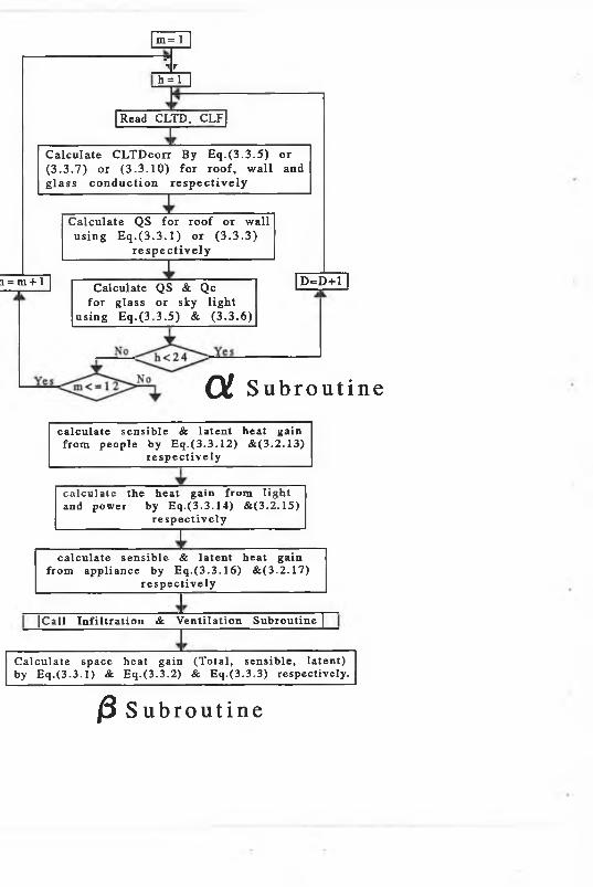
m = I |
r ,>-11
h == » 1
Read CLTD. CLF
Calcul ate CLTDcorr By Eq . (3 .3 .5) or ( 3 . 3 . 7) or ( 3 . 3 . 10) for roof , wal l and g l a s s con du c t i on r e s p e c t i v e ly
Calcul ate QS for roof or wal l us ing E q . (3 .3 .1 ) or ( 3 . 3 . 3 )
r e s p e c t i v e l y
a = m + 1 Calculate QS & Qcfor glass or sky l ight
using Eq.(3 3.5) & (3.3 .6)
D=D+1
0 1 S u b r o u t i n e
c a l c u l a te se n s ib le & l a t e n t h e a t ga in f ro m p e o p le by E q . ( 3 .3 .1 2 ) & (3 .2 .1 3 )
r e s p e c t i v e l y
c a l c u l a te the h e a t g a in f ro m l ig h t and pow er by E q .(3 .3 .1 4 ) & (3 .2 .15 )
r e s p e c t i v e l y
c a l c u l a te s e n s ib le & l a t e n t h e a t g a in f rom a p p l ia n c e by E q . ( 3 .3 .1 6 ) & (3 .2 .1 7 )
r e s p e c t i v e l y
|C a l l I n f i l t r a t i o n & V e n t i l a t io n S u b ro u t in e |
C a lc u l a t e space h e a t ga in (T o ta l , s e n s ib le , l a t e n t ) by E q .(3 .3 .1 ) & E q .(3 .3 .2 ) & E q .(3 .3 .3 ) respec tive ly .
j8 S u b r o u t i n e

the user has to enter all information for the wall and glass if it is available except the
temperature difference. For the floor there are four allowable combinations:
1 - All inputs equal to zero it the roof is internal and there is no temperature
difference.
2 - 4 The user has to input all inputs and for the floor type takes value "1" for
internal or "2" for solid ground or "3" for basement floor.
The user also has to input number of people and their activity degree according
to table 3 chapter 26 in ref. [7] and the light wattage according to their types in watt per
square meter. For calculating the heat gains from power and appliances the user has to
enter the total power and appliances if they are available, the efficiency, load factor and
use factor which should not equal zero and if the user gives any one factor a zero value
then the program automatically assigns a unity value. The heat gain from infiltration can
be calculated using two methods for calculating the flow rate of the air as mentioned
before, then the user has to select the type of infiltration, "1" for air change method and
if it is selected the user also has to enter number if air changes, or "2" for crack method
and if selected the user has to enter the crack length. Because in air conditioning the
ventilation load is added to the cooling loads, the user has to enter the ventilation
information if the ventilation is needed. "1" for air changes method and if it is selected
the user also has to enter number if air changes, or "2" for CFM per person method and
if it is selected the user has to enter the CFM per person.
When the user completes the input data, he has a choice to continue for anther
space , anther storey, another building and so on by following the commands in the help
line. Then the calculation of the elements of the heat gains begin as shown in Fig.(3.3)
and Fig.(3.7) which may be explained as follows:
1 - Read all information fixed in user place and client place setup which are
user name and his address, client place and his address, name of the
project, place latitude, the outside temperature and relative humidity in
summer and winter and safety factors for cooling and heating loads,
76
number of buildings and closing and opening hours.
2 - Select the method of calculation procedure, "Room by Room" or "Whole
Building".
3 - Open loop for building numbering from 1 to the number of buildings
4 - Enter building information using the building entry input data menu.
5 - Open loop for storey numbering from 1 to the number of storeys.
6 - Open loop for space numbering from 1 to the user choice by pressing
"ESC" key.
7 - Enter space information using the space entry input data menu.
8 - If "Room By Room" method is selected calculate the cooling load for the
space using space cooling load subroutine which is shown in Fig.(3.7) and
displays the results on the screen, and print out if the user wants that. If
"Whole Building" method is selected go to the next input for another space
without calculations.
9 - If the second option is selected ("Whole Building" method) calculate the
cooling load for each space according to the space cooling load subroutine
for all rooms in the buildings.
10 - Save the inputs and outputs for printing out the reports or redisplaying or
for checking and modifying.
3.5 PSYCHROMETRIC CHART PROGRAM:
The psychrometric chart is one of the most valuable tools available for air
conditioning engineer. It is a way of graphically representing the properties of moist air,
the knowledge about this chart is required for the design of heating, ventilating and air
conditioning (HVAC) systems. This chart provides engineers information on properties
of moist air rapidly and conveniently.
The psychrometric chart program is more than an electronic display of the
conventional printed chart. For example, it can quickly display numerical values of all
properties at any selected point without interpolation. These points can be labelled for
77

future reference, and reports of their properties can be displayed on the screen or printer.
Additionally, the program allows psychrometeric processes to be analyzed. The lines for
all standard psychrometric processes, such as heating, cooling humidification, mixing
and so on, are displayed on the chart by simple user commands. Once displayed, reports
giving heating rates, cooling rates, air quantities and water removal or addition rates can
be reported.
Psychrometric chart program goes beyond the capabilities of printing the charts.
Although the initial display is the standard ASHRAE sea level chart, this can be
changed by the user to show a chart for any elevation or pressure and for any range of
dry bulb temperature, and can be specified in either Imperial or SI units.
These features will allow the user to carry out psychrometric analysis of air
conditioning systems more conveniently, accurately and quickly than before. The user
of the program will find that the ease of doing even complex analysis will lead to
improved design. The objective of creating a psychrometeric program is to enable the
rapid calculations, on a normal personal computer without the need for tables or charts.
For calculating the properties of moist air, number of sources [7,8,28-36] have
been consulted, and equations given in reference [7] appears to give the more accurate
values.
3.5.1 T h e r m o d y n a m i c p r o p e r t i e s o f m o i s t a i r :
The following symbols are used throughout the equations:
- tdb : Dry bulb temperature, [ °C ]
- twb : Wet bulb temperature, [ °C ]
- tdp : Dew point temperature, [ °C ]
- Tk : Kelvin temperature, [ °K = °C + 273.16 ]
- PB : Barometric pressure, [ kPa ]
- O : Relative humidity, [ % ]
- Ra : Gas constant for dry air, [ J/(kg.°k) ]
78

- V : Specific volume of moist air, [ m3/kg ]
- W : Humidity ratio of moist air, [ kgw/kga ]
- W s : Humidity ratio of moist air at saturation, [ kg^kg,, ]
- P ws: Saturated vapour pressure [ kPa ]
- Pw : Partial vapour pressure [ kPa ]
- Pws* : Saturated vapour pressure at wet bulb temperature [kPa]
- h : Enthalpy of moisture air. [ k j/kg ]
- ha : Enthalpy of dry air. [ k j/kg ]
- hw : Enthalpy of water vapour. [ k j/kg ]
Various Formulas:
The purpose of comparing working formulas from several sources is to obtain
the most appropriate formula for solving any problem. Working formulas when design
calculations were carried out it was found that there is difference between the values
calculated using different formulas and the values obtained from the psychrometric chart
The following approach for calculating the moist air properties is based upon the
Tetens relationship [36] for saturation vapour pressure and the psychrometric equation.
Tetens method closely approximates the internationally accepted relationship of Goff-
Gratch [28-30], Based on the latter and more accurate measurements, Hyland and
Wexler’s relationship (1983a) as given in ASHRAE [7] gives a vapour pressure equation
for the temperature range 0 to 100 °C. For the temperature range -50 to 0 °C another
comparison have been done between Tetens [36], Goff-Gratch [28], CIBSE Guide [8]
and Wexler-Hyland [7],
These relationships are based upon pure vapour phase of water, rather than moist
air , over plane surface which leads to an error of approximately 0.5 percent.
Saturated vapour pressure relationships :
The determination of the saturation vapour pressure is the most important
79
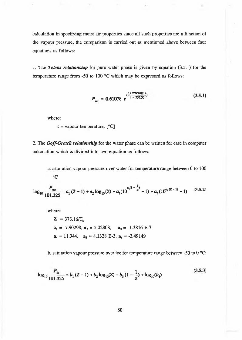
calculation in specifying moist air properties since all such properties are a function of
the vapour pressure, the comparison is carried out as mentioned above between four
equations as follows:
1. The Tetens relationship for pure water phase is given by equation (3.5.1) for the
temperature range from -50 to 100 °C which may be expressed as follows:
, 17.2693882 r ^
P = 0.61078 e ' + 23730 ( )w s
where:
t = vapour temperature, [°C]
2. The Goff-Gratch relationship for the water phase can be written for ease in computer
calculation which is divided into two equation as follows:
a. saturation vapour pressure over water for temperature range between 0 to 100
°C
10810T o n 2 5 = a , ( z " +a2lo8io(Z) * <*3(iov l ~2>- 1 ) *o5(10“< *-u - 1) a s -2)
where:
Z = 373.16/Tk
a x = -7.90298, a2 = 5.02808, a3 = -1.3816 E-7
a4 = 11.344, as = 8.1328 E-3, a,; = -3.49149
b. saturation vapour pressure over ice for temperature range between -50 to 0 °C:
lQgl° 10nt25 =bi ( Z ~ 1)+ b2 ^ lo C 2) + fc3 i 1 - | ) + logio(*4> (3 5 3)
80
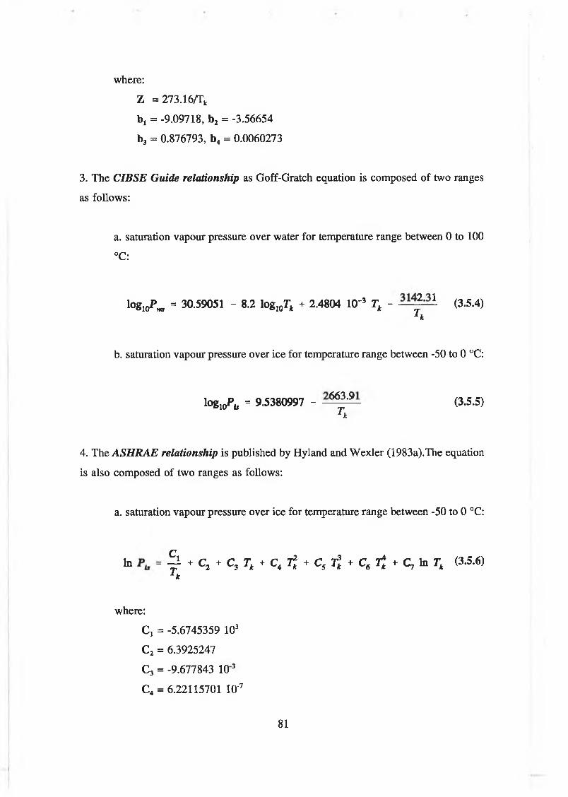
where:
Z = 273.16/Tk
b x = -9.09718, b 2 = -3.56654
b 3 = 0.876793, b 4 = 0.0060273
3. The CIBSE Guide relationship as Goff-Gratch equation is composed of two ranges
as follows:
a. saturation vapour pressure over water for temperature range between 0 to 100
°C:
togioP^ = 30.59051 - 8.2 log107; + 2.4804 10"3 Tk - — 2—1 (3.5.4)T k
b. saturation vapour pressure over ice for temperature range between -50 to 0 °C:
togioPfc = 9.5380997 - - 663'9- (3.5.5)^ k
4. The ASH RAE relationship is published by Hyland and Wexler (1983a).The equation
is also composed of two ranges as follows:
a. saturation vapour pressure over ice for temperature range between -50 to 0 °C:
1" ^ + Ca + c, Tt + C4 7f + C5 f t * Cc 7i * C7 to r, (3.5.6)L k
where:
Cx = -5.6745359 103
C2 = 6.3925247
C3 = -9.677843 103
C4 = 6.22115701 10'7
81

Cs = 2.0747825 IO'9
C6 = -9.484024 IO13
C7 = 4.1635019
b. the saturation vapour pressure over water for the temperature range of 0 to
200 °C:
1” - - F * C> * CK Tk + Cn 1Ì * Cn ^ » C „ In Tt (3.5.7)
where:
C8 = -5.8002206 103
C9 = 1.3914493
C10 = -4.8640239 10'2
Cu = 4.1764768 10'5
C12 = -1.4452093 10’8
C13 = 6.5459673
Fig.(3.8) to Fig.(3.17) and Table (3.8) show the comparison results of the
calculated saturation vapour pressures based on equations (3.5.1) - (3.5.7) as a function
of temperature. There is excellent agreement between the four equations in the range 0
to 60 °C, Fig.(3.13), Fig.(3.14) and Fig (3.15). Below 0 °C there is obvious considerable
difference between the Tetens relationship and those of others, and above 60 0 the
Tetens’ equation deviates from the other three but never by more than 1 percent. There
is better agreement between the ASHRAE and CIBSE equations than that with the Goff-
Gratch equation. The obvious advantage of Tetens equation is the ease of calculation.
A computer program is developed for these comparison. For the psychrometeric
properties, the ASHRAE equation is selected because it gives more accurate results for
the moist air properties when they are compared with the Standard Psychrometric charts.
Also similar comparison between other sources have been done for old equations of
Goff-Gratch, Wexler-Greenspan, ASAE standard and Tetens by Albert Weiss (1977)
[36].
82

0.0178
Fig. (3.8) Saturation Vapour Pressure for Fig. (3.9) Saturation Vapour Pressure for temperature range -50 to -41 °C temperature range -40 to -31 °C
T a ta n a Eq.+ G o ff-G tm to h Eq, * C IB S l I q .
AHHBA1 I q .
Fig. (3.10) Saturation Vapour Pressure fo r Fig. (3.11) Saturation Vapour Pressure for temperature range -30 to -21 °C temperature range -20 to -11 °C
Fig. (3.12) Saturation Vapour Pressure for Fig. (3.13) Saturation Vapour Pressure for temperature range -10 to -1 °C temperature range 0 to 20 °C
83

i S H U l I q .2 ---------------------------------21 2 3 2 5 2 7 2 9 31 3 3 3 6 3 7 3 9
t fC]Fig. (3.14) Saturation Vapour Pressure fo r Fig. (3.15) Saturation Vapour Pressure for
temperature range 21 to 40 °C temperature range 41 to 60 °C
Fig. (3.16) Saturation Vapour Pressure fo r Fig. (3.17) Saturation Vapour Pressure for temperature range 61 to 80 °C temperature range 81 to 100 °C
84
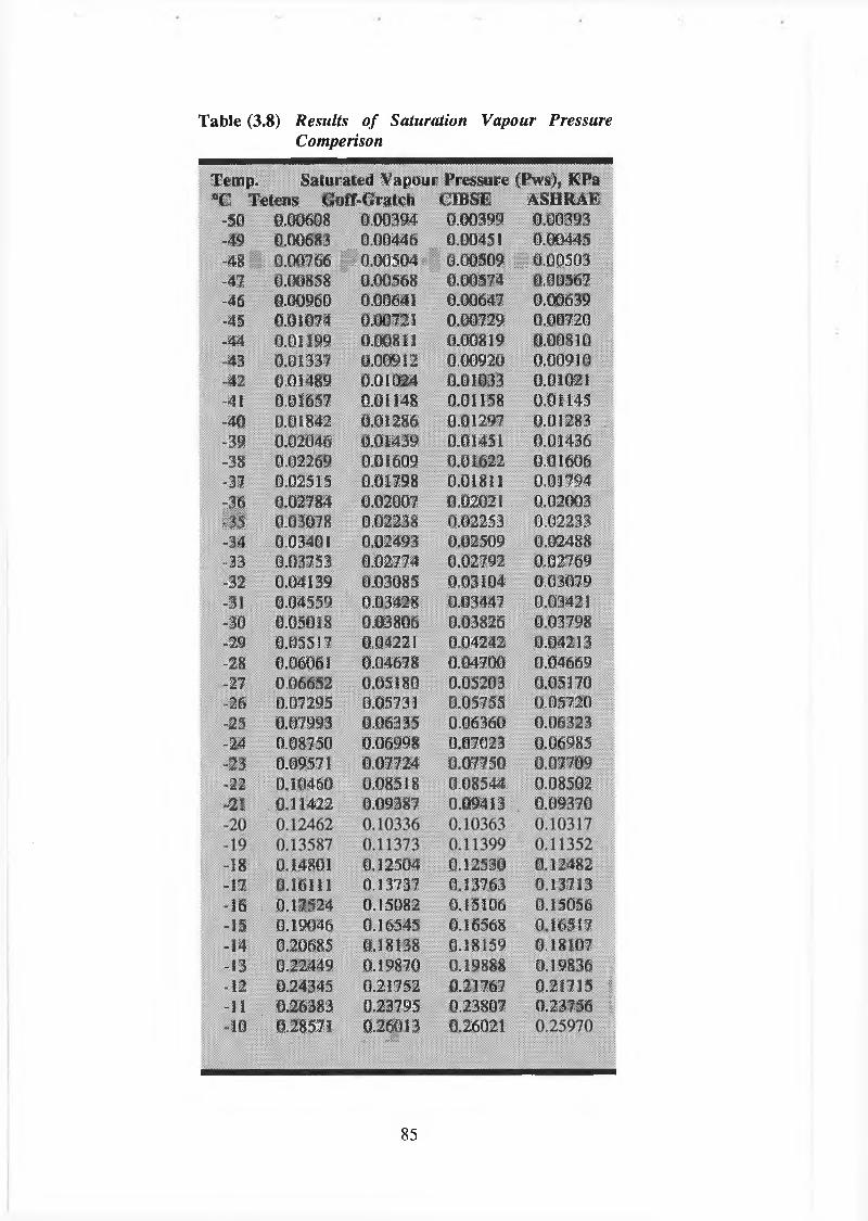
Table (3.8) Results o f Saturation Vapour Pressure Comperison
Temp. Saturated Vapour Pressure (Pws), KPa°C Tetens Goff-Gratch CIBSE ASHRAB
-50 0 .00608 0 .00394 0 .00399 0 .00393-49 0.00683 0 .00446 0.00451 0 .00445-48 f t . 0 .00766 |V 0 .00504 ::!-0 .00509 f t 0 .00503-47 0.00858 0 .00568 0 .00574 0 .00567-46 0 .00960 0.00641 0 .00647 0 .00639-45 0 .01074 0.00721 0 .00729 0 .00720-44 0 .01199 0.00811 0 .00819 0 .0081043 0.01337 0 .00912 0 .00920 0 .0091042 0 .01489 0 .01024 0 .01033 0.01021
-41 0.01657 0 .01148 0.01158 0 .01145-40 0.01842 0 .01286 0 .01297 0 .01283 :-39 0 .02046 0 .01439 0.01451 0 .01436-38 0 .02269 0 .01609 0 .01622 0 .01606-37 0.02515 0 .01798 0.01811 0 .01794-36 0 .02784 0 .02007 0.02021 0 .02003M 0 .03078 0.02238 0.02253 0 .02233-34 0.03401 0 .02493 0 .02509 0 .02488•33 0.03753 0 .02774 0 .02792 0 .02769-32 0 .04139 0 .03085 0 .03104 0 .03079-31 0 .04559 0 .03428 0.03447 0.03421-30 0.05018 0 .03806 0 .03826 0 .03798-29 0.05517 0.04221 0 .04242 0 .04213-28 0.06061 0 .04678 0 .04700 0.04669-27 0 .06652 0 .05180 0.05203 0 .05170•26 0.07295 0.05731 0.05755 0 .05720-25 0 .07993 0 .06335 0 .06360 0 .06323-24 0.08750 0 .06998 0.07023 0 .06985-23 0.09571 0 .07724 0 .07750 0 .07709-22 0 .10460 0 .08518 0.08544 0.08502-21 . 0 .11422 0 .09387 0 .09413 . 0 .09370
-18 0.14801 0 .12504 0 .12530 0 .12482-17 0.16111 0.13737 0 .13763 0 .13713•16 :: 0 .17524 0 .15082 0 .15106 0.15056-15 0 .19046 0 .16545 0.16568 0 .16517-14 0 .20685 0.18138 0 .18159 0 .18107-13 0 .22449 0 .19870 0.19888 0.19836-12 0.24345 0 .21752 0.21767 0 .21715-11 0 .26383 0.23795 0.23807 0 .23756«10 ' 0.28571 0 .26013 0.26021
. : ™ - ■m m
85
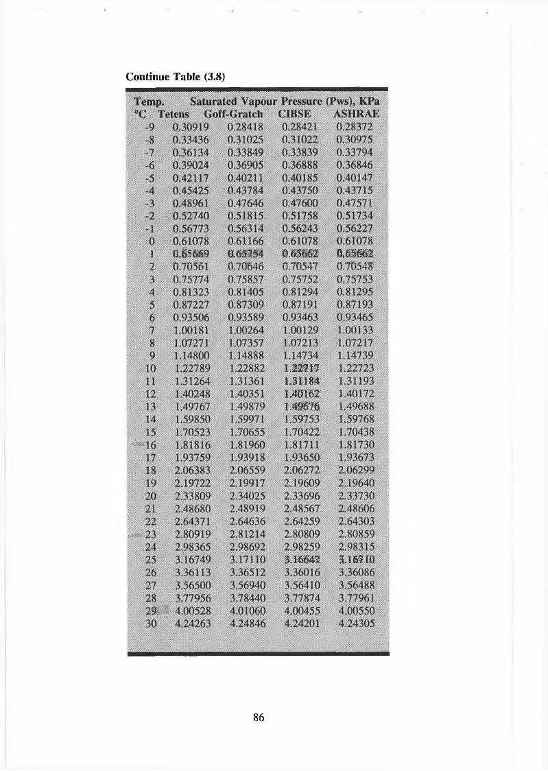
Continue Table (3.8)
1 0 ¿5669 0.65754 0.65662 0.65662^ > v /-V ^ ^ /-X s W , V A ^ n ^ i r , /A - n A i- J A
1.227171.31184
1.40162
1.49676
¡ÎftiWS
W 8 M
3.16647 3.16710
i l l
86

Continue Table (3.8)
1*49213
7.77777 7 .78025
48 11.16129 11.18069 11.16217 11.1659149 11.73555 11.75574 11.73622 11.7401550 12.33504 12.35596 12.33543; 12,3395751 12.96068 12.98230 12.96070 12.9650352 13.61339 13.63562 13.61294 13.6174653 14.29414 14.31691 14.29309 14.2978254 15.00390 15.02713 15.00213 15.0070355 15.74368 15.76724 15.74104 15.7461456 16.51451 16.53830 16.51083 16.5161357 17.31746 17.34131 17.31256 17.3180458; 18.15361; 18.17735 18.14728 18.1529459 19.02408 19.04753 19.01610 19.0219060 19.93000 19.95296 19.92012 19.9260961 20.87256 20.89477 20.86050 20.8666362 21.85294 21.87418 21.83840 21.8446863 22.87238 22.89235 22.85503 22.8614264 23.93213 23.95049 23.91161 23.9181265 25.03348 25.04987 25.00940 25.0159966 26.17775 26.19177 26.14967 26.15637
27.37750 27.33374 27.3405028.60845 28.56295 28.5697129.88594 29.83866 29.8454831.21133 31.16228 31.16908
68 28.6004569 29.8816770 31.21138
87

Continue Table (3.8)
73 35.50637 35.48958 35.43494 35.4415474 37.04511 37.02134 36.96471 36.9711875 38.64004 38.60847 38.54982 38.5561776 40.29279 40.25245 40.19184 40.1979977 42.00503 41.95512 41.89237 41.8983778 43.77847 43.71788 43.65306 43.6587879 45.61487 45.54250 45.47557 45.4810380 47.51598 47.43079 47.36161 47 .3667281 49.48363 49.38423 49.31291 49 .3176482 51.51967 51.40483 51.33124, 51.3356383 53.62598 53.49423 53.41839 53.4223084 55.80449 55.65438 55.57619 55.5796485 58.05714 57.88713 57.80651 57.8095086 60.38594 60.19424 60.11124 60.1136687 62.79292 62.57779 62.49231 62.4942588 65.28016 65.03964 64.95169 64.9530189 67.84975 67.58198 67.49136 67.4920390 70.50387 70.20655 70.11336 70.1134491 73.24467 72.91566 72.81974 72 .819069 2 76.07441 75.71125 75.61259 75 .6113493 78.99533 78.59551 78.49408 78 .4920694 82.00975 81.57059 81.46634 81.463609 5 85.12000 84.63883 84.53156 84.52819
98 95.04988 94.42406 94.30754 94.3021799 98.56776 97.88705 97.76733 97.76137
100 102:19382 101.45469 101.33155 101.32500
88

3.5.2 F orm ulation of psychrom etric pro perties:
To a first approximation, air and
water vapour may be considered as 100 9 5perfect gases because the temperature0.9
of dry air is usually very high ^
compared with its critical temperature, 0 0<
and because the partial pressure of the^> 0.75
water vapour is very low compared 0.7
with its critical pressure. Therefore,
atmospheric air can be considered as
a mixture of perfect gases. The
equations used in the program were
obtained mainly from refs. [7,8]: Fig. (3.18) Variation o f barometric pressurewith altitude
Z [m]
Barometric pressure:
Most psychrmetric charts published are for sea level only, the accurate values of each
spaces may be corrected by multiplying by appropriate correction factors. Here, using
the barometric pressure for each altitude the user can get accurate values of the
psychrometric properties of moist air. Fig.(3.18) which gives the relationship between
height above sea level and barometric pressure, is drawn from the equation (3.5.8):
P *"Z (3.5.8)1000 BP b = P o e
where:
pB = barometric pressure at altitude Z, [KPa]
p0 = barometric pressure at see level (=101.325), [KPa]
p = density of air (= 1.20), [Kg/m2]
gn = acceleration due to gravity (=9.81), [m/s2]
Z = Altitude above see level, [m]
89

Saturation vapour pressure:
Saturated air is that mixture in which the water vapour is saturated; that is when the
partial pressure of vapour is the saturation pressure of water at the temperature of air.
Equations (3.5.6) and (3.5.7) are used to calculate the saturation vapour pressure in the
program.
Relative humidity:
The moisture content in the air is commonly indicated by the relative humidity <3>,
defined as the ratio of the mass of water vapour present in a certain volume of air to
that present in an equal volume of saturated air at the same temperature and total
pressure, i.e.
Humidity ratio:
The humidity ratio (W), indicates the composition of air, it is defined as the ratio of
the mass of water vapour to that of dry air in the mixture, i.e.
4> = (3.5.9)
Using the perfect gas relations, the relative humidity can be expressed as:
(3.5.10)
w (3.5.11)
Applying the perfect gas relations,
(3.5.12)
According to Dalton’s rule;
P = P a + P w
and the humidity ratio can be expressed as:
(3.5.13)
90

(3.5.14)
vK p b
V R a T.— = (1 + 1.6078 W) (3.5.15)
Specific enthalpy:
The enthalpy of moist air per kilogramme of dry air can be evaluated as the sum of the
individual partial enthalpies of the components. Therefore, it can be written as:
where:
ha = the specific enthalpy for dry air, [KJ/Kg].
hg = the specific enthalpy for saturated vapour at the temperature of the mixture
For most engineering applications, it is sufficiently accurate to assume that the constant
pressure specific heat Cpa of dry air is constant over the relatively limited temperature
range of air conditioning processes. Therefore, its value can be taken as that of air at
0 °C (i.e. Cpa = 1 [KJ/Kg°C]). Then the moist air enthalpy becomes:
Wet bulb temperature twb:
The psychrometer consists of two thermometers; one thermometer’s bulb is covered
by a wick that has been thoroughly wetted with water. When the wet bulb is placed in
an equilibrium temperature called the wet bulb temperature which is defined as a unique
property of a given moist air sample independent of measurement techniques. Equation
h = h + W ha g(3.5.16)
K C pa tdb(3.5.17)
hg = 2501 + 1.805 t^ (3.5.18)
h = U + W (2501 + 1.805 t j (3.5.19)
91

(3.5.20) given in ASHRAE [7] as follow:
where the properties Ws*, hw* and hs* are functions only of the temperature t^ for a
fixed value of pressure; and the value of twb which satisfies equation (3.5.20) for given
values of h, W, pws is the wet bulb temperature;
h*w = 4.186 twb (3.5.21)
*w ; = 0.62198 P~' (3.5.22)
P B ~ P m
by using numerical analysis to solve equation (3.5.20) using Equations (3.5.21) and
(3.5.22) and (3.5.6), (3.5.7) by replacing t ^ instead of tdb, the wet bulb temperature is
obtained.
Dew point temperature:
The dew point temperature can be calculated directly by using one of the following
equations:
For the dew point temperature range of 0 to 93 °C:
tjp = A + B a + C a 2 + D a3 + E p°w19M (3.5.23)
and for temperature below 0 °C:
*dp = 6 09 + 12 608 a + 0 4959 «2 (3.5.24)
where
tdp = dew point temperature, [°C]
a = In pw
A =6.54
B = 14.526
C = 0.7389
D =0.09486
h + (W* - W) h i = h*s (3.5.20)
92
I
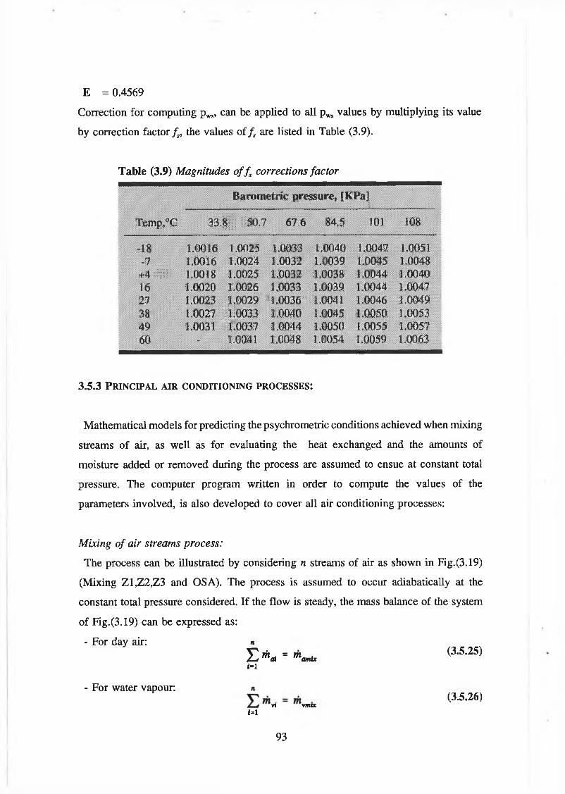
E = 0.4569
Correction for computing pws, can be applied to all pws values by multiplying its value
by correction factor f s, the values of f s are listed in Table (3.9).
Table (3.9) Magnitudes o f f corrections factor
Barometric pressure, [KPa]s i
Temp*0C 33. ..... ...... ’ 67.6 84.5 101 108
-18 1.0016 1.0025 1.0033 1.0040 1.0047 1.0051-7 1.0016- 1.0024 1.0032 1.0039 1.0045 1.0048+4 ifj. i- 1.0018 1.0025 1.0032 1.0038 1.0044 1.004016 1.0020 1.0026 1.0033 j 1.0039 1.0044 1.004727 1.0023 1.0029 11.0036. 1.0041 1.0046 1.004938 1.0027 ¡¡¡0033 1.0040 1.0045 1.0050 1.005349 1.0031 11113037 1.0044 1.0050 1.0055 1.005760 - 1.0041 1.0048 1.0054 1.0059 1.0063
3.5.3 P r i n c i p a l a i r c o n d i t i o n i n g p r o c e s s e s :
Mathematical models for predicting the psychrometric conditions achieved when mixing
streams of air, as well as for evaluating the heat exchanged and the amounts of
moisture added or removed during the process are assumed to ensue at constant total
pressure. The computer program written in order to compute the values of the
parameters involved, is also developed to cover all air conditioning processes:
Mixing o f air streams process:
The process can be illustrated by considering n streams of air as shown in Fig.(3.19)
(Mixing Z1,Z2,Z3 and OSA). The process is assumed to occur adiabatically at the
constant total pressure considered. If the flow is steady, the mass balance of the system
of Fig.(3.19) can be expressed as:
- For day air: nE * 1 = " a m * (3*5'25)¡=1
- For water vapour:
i=l
93
(3.5.26)VI V7TUX
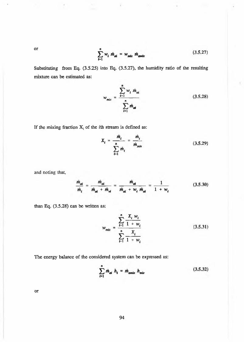
or nI > i ( 3 -5 - 2 7 )1=1
Substituting from Eq. (3.5.25) into Eq. (3.5.27), the humidity ratio of the resulting
mixture can be estimated as:
X > i <w = ±1______ (3.5.28)
mix n
1=1
If the mixing fraction Xi of the zth stream is defined as:
m { mtX = 1 - '' ' « “ * (3.5.29)
E ™ <i=imix
and noting that,
+ + Wi 1 + Wi
• Xt wt
than Eq. (3.5.28) can be written as:
_ M 1 + W| " XE — — H i +
i=l
(3.5.30)
^ (3'5-31)
The energy balance of the considered system can be expressed as:
X > « k i = hmix
or
9 4
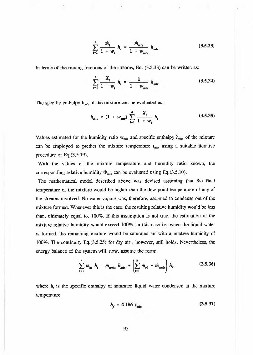
JL mt m_w„ ^ (3.5.33)fitix
v -> "*1 ^ "'m ix h
h i + w, 1 " i + -
In terms of the mixing fractions of the streams, Eq. (3.5.33) can be written as:
f — A !----------------------- (3-5-34)m 1 + 1 ♦
The specific enthalpy hmix of the mixture can be evaluated as:
a ‘ « ’j t A * ,M 1 + w t
hn*c = d + V! — — A. (3*5*35)
Values estimated for the humidity ratio wmix and specific enthalpy h ^ of the mixture
can be employed to predict the mixture temperature tmbt using a suitable iterative
procedure or Eq.(3.5.19).
With the values of the mixture temperature and humidity ratio known, the
corresponding relative humidity can be evaluated using Eq.(3.5.10).
The mathematical model described above was devised assuming that the final
temperature of the mixture would be higher than the dew point temperature of any of
the streams involved. No water vapour was, therefore, assumed to condense out of the
mixture formed. Whenever this is the case, the resulting relative humidity would be less
than, ultimately equal to, 100%. If this assumption is not true, the estimation of the
mixture relative humidity would exceed 100%. In this case i.e. when the liquid water
is formed, the remaining mixture would be saturated air with a relative humidity of
100%. The continuity Eq.(3.5.25) for dry air , however, still holds. Nevertheless, the
energy balance of the system will, now, assume the form:
n / n \
E ™ * h i = h n * + E ™ W -1=1 V<=1
hf (3.5.36)
where hf is the specific enthalpy of saturated liquid water condensed at the mixture
temperature:
hf = 4.186 (3.5.37)
95

In terms of the mixing fractions of the streams and humidity ratios, Eq.(3.5.36) assumes
the form:
1_1 + w. h mix +
mix
» X f W t
f t 1 + w i
(3.5.38)
For the known relative humidity of the mixture (i.e. <3>mU=100%) and by employing
Eq.(3.5.14) and(3.5.19), the temperature of the mixture formed can be estimated from
Eq.(3.5.19) using an iterative process.
The values of and t ^ can be used to evaluate the humidity ratio wmix of the
mixture. The mass rate of the condensed moisture, per unit mass flow rate of dry air,
is then:
m w =X. w,
m amix(3.5.39)
Heating and cooling processes:
In terms of initial state of the air, defined by the values of any two parameters which
can define the state point (i.e. tdbl and <J>j), analysis of the heating and cooling precesses,
in order to achieve a desired final temperature tdb2, is aim at:
I. evaluating the energy interactions as heat, and
II. predicting the properties at the final state reached.
Constant total pressure heating does not change the humidity ratio and, therefore, the
water vapour partial pressure remains unaltered. However, the relative humidity
decreases. From the energy balance of the system of Fig.(3.19), the quantity of heat
added, per unit flow rate of dry air, during the process considered, can be evaluated as:
= *2 “ h i (3.5.40)
The specific enthalpy ht can be computed in terms of the values of any two parameters
which can describe the state point (tdM, Oj). As in the process concerned, w2 and wt are
equal, h2 and the final relative humidity can be estimated as functions of the known
96

values of w2 and tdb2.
Z3 Z2 Z1
3 ’ 4 ’ 4”
Fig. (3.19) Domestic Air Conditioning System with Air Handling Unit (AHU)
Constant pressure cooling does not alter the humidity ratio if the air is cooled to a
temperature tdb3, higher then the dew point temperature, i.e. if no condensation of water
vapour ensues (process 2-3). In this case, the relative humidity of air rises. The amount
of heat interaction can be calculated using EQ.(3.5.40) and the final relative humidity
<2>3 can be estimated as a function of tdb3 and w3(=w2).
Cooling to a temperature below the dew point temperature (process 2-3’) results in
moisture condensation and lowering the humidity ratio of the air. The air become
saturated (i.e. <&3.=100%). The amount of moisture condensed, per unit flow rate of dry
air, during the process is w2-w3.. The amount of energy transferred as heat, per unit rate
of flow of dry air, can be calculated from:
02-3' = 0*3' “ *2) + (w3' _ (3.5.41)
where hf is the specific enthalpy of saturated liquid water at tdb2.
97

Humidifying process:
Two methods are commonly used to increase the humidity ratio of air, namely
adiabatic evaporation or evaporation with heat addition. In the adiabatic evaporation
process, air passes through a spray of water in a thermally-insulated system, similar to
that shown in Fig.(3.19). Some of the water evaporates and the humidity ratio of the air
increases, simultaneously, the temperature of the air drops. Such a process runs along
a line of constant wet bulb temperature on a psychrmetric chart. The humidity ratio
could increase to a limiting value at which the air becomes saturated (state 4). i.e. when
the temperature of the air drops to the adiabatic saturation temperature.
For a selected value for the final humidity ratio w4, the amount of water that evaporates
during the process, per unit mass flow rate of dry air, is w4-w3.
The energy balance of the system is expressed by EQ.(3.5.40) which can be employed
to estimate the value of tdb4. The final relative humidity 0 4 can, then, be evaluated in
terms of tdb4 and w4.
During evaporation accompanied by heating, air is passed through a spray of water
while, simultaneously, heat is transferred to the system. The cooling due to evaporation
opposes the rise in temperature resulting from heat addition. The combined effect,
therefore, may be either a net reduction in temperature, as shown by process 3-4’ in Fig.
(3.19), or a net increase in temperature as illustrated by process 3-4". In process 3-4’,
the relative humidity <i> rises, whereas in process 3-4", the value of <J> drops. Depending
upon the final values of humidity ratio and relative humidity (or alternately the
temperature) desired, the corresponding temperature ( or relative humidity) can be
estimated. The energy balance of the system involved can be used to compute the
amount of heat added, per unit mass flow of dry air, as:
$3-4 = K ~ (*3 + (W4 “ W3> hp (3.5.42)
where hf is evaluated at the final temperature tdb2.
98

PSYCHROMETRIC CHARTBarometric pressure 100.4786 KPa
0 - ‘ M W f U ' W M C I I ® 0 - M O l * y ' C l ' > J O » ( 0 0 - , W W Ì O Ì $ s J Ù « ) 0 - W O < t U ' 5 i ' J a ( 0 0 - ‘ K 3 Ó l l ( > ( S N j O l ( 0 0
D R Y B U L B T E M P E R A T U R E (£)
.035
.034
.033
.032
.031
.03
.029
.028
.027
.026
.025
.024
.023
.022
.021
.02
.019
.018.017
.016
.015,014
.013
.012
.011
.01
.009
.008
.007
.006
.005
.004
.003
.002
.001
0
Fig. (3.20) Representation o f Air Conditioning Processes on The Psychrometric chart.
HUMI
DITY
RATIO
(KGw
/KGa
ir)
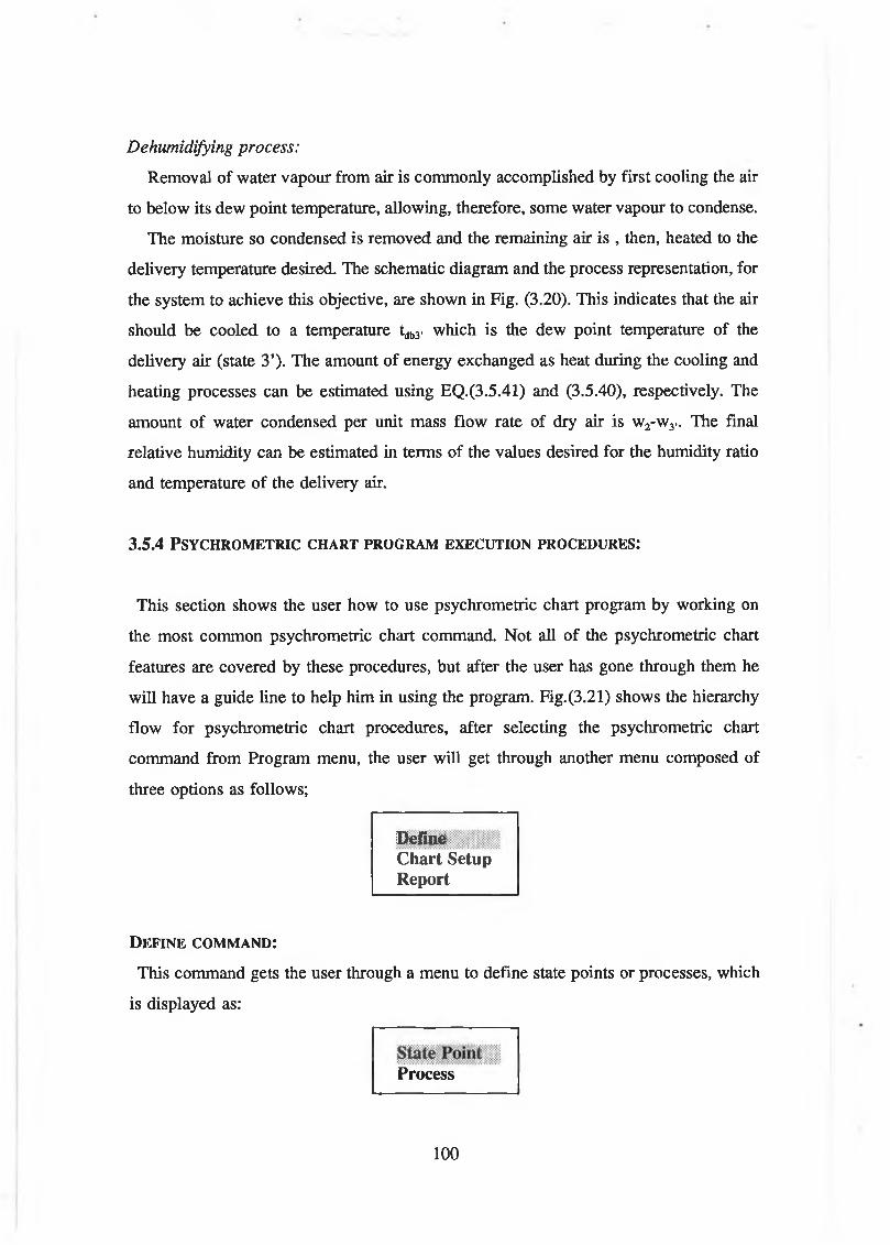
Dehumidifying process:
Removal of water vapour from air is commonly accomplished by first cooling the au
to below its dew point temperature, allowing, therefore, some water vapour to condense.
The moisture so condensed is removed and the remaining air is , then, heated to the
delivery temperature desired. The schematic diagram and the process representation, for
the system to achieve this objective, are shown in Fig. (3.20). This indicates that the air
should be cooled to a temperature tdb3. which is the dew point temperature of the
delivery air (state 3’). The amount of energy exchanged as heat during the cooling and
heating processes can be estimated using EQ.(3.5.41) and (3.5.40), respectively. The
amount of water condensed per unit mass flow rate of dry air is w2-w3.. The final
relative humidity can be estimated in terms of the values desired for the humidity ratio
and temperature of the delivery air.
3.5.4 PSY CH RO M ETRIC CHART PROGRAM EXECUTION PROCEDURES:
This section shows the user how to use psychrometric chart program by working on
the most common psychrometric chart command. Not all of the psychrometric chart
features are covered by these procedures, but after the user has gone through them he
will have a guide line to help him in using the program. Fig. (3.21) shows the hierarchy
flow for psychrometric chart procedures, after selecting the psychrometric chart
command from Program menu, the user will get through another menu composed of
three options as follows;
Delink Chart Setup Report
D e f i n e c o m m a n d :
This command gets the user through a menu to define state points or processes, which
is displayed as:
Process
100

HVACSYSMain Menu U s e r In ter face
P r o g r a m P u l l - d o w n M e n u |
P s y c h r o m e t r i c c h a r t !
C h a r t S e t U p |
? -
> R e p o rt~ ~ |- frj D XF F ile 'k .
D e f i n e JM enu Input for
U n i t s , A l t i t u d e D r y B u l b T e m p e r a t u r e R a g e H u m i d i t y R a t i o R a n g e P a r a m e t e r s L i n e s S h o w s P a r a m e t e r s L a b e l s S h o w s
^ m e ^ P o i n J TrïïcTsTj
Pt = 1 Prc = 1
S t a t e P o i n tM e n u I n p u t
I n p u t t w o p a r a m e t e r s o f f i v e P l u s S t a t e P o i n t L a b e l
A c c o r d i n g t o a l l o w a b l e i n p u t c o m b i n a t i o n s
T a b l e ( 3 . 4 . 3 ) c a l c u l a t e
t h e o t h e r p a r a m e t e r s
G e n e r a l H e a t i n g Co i l C o o l i n g Coi l Z o n eH u m i d i f i c a t i o nM i x i n gC o l l e c t i n g
Pr c = P r c +1
/ O u t p u t P o r t A
~ i _
Ç e x Î Q
J r J t
P r o c e s s M e n u I n p u t
I n p u t t h e a l l o w a b l e c o m b i n a t i o n f o r p r o c e s s
A c c o r d i n g t o a l l o w a b l e i n p u t c o m b i n a t i o n s c a l c u l a t e t h e E n e r g y B a l a n c e s
Fig. (3.21) Flow Diagram of The Psychrometric Chart Programme Procedures

I) State point option:
This option lets the user to define a state point on the psychrmetric chart by inputting
two parameters, then the user obtains the other parameters. Since the State Point
command is highlighted, meaning that is selected from last menu, depressing <enter>
brings up the following entry dialogue box:
State Point No. 1 input on chartwith barometric pressure 101.325 [KPa]
State point label iillggpDry bulb temperature
©©
[°C]Relative humidity 0 [%]Wet bulb temperature 0.00 [°C]Dew point temperature 0.00 [°C]Humidity ratio 0.00000 [kgw/kg jEnthalpy 0.000 IkJ/kglSpecific Volume Ì M U [m3/kg]Partial Vapour pressure ■ l l Ü i l [kPa]Saturation Vapour pressure [kPa]
There are only 13 cases to define a state point, and all the cases are solved by using
the developed program. Table (3.10) shows how for two given parameters, in addition
to barometric pressure PB, to compute the others parameters. Also there is help guide
line to ease the inputs, the output directly will appear on the dialogue box.
Table (3.10) The Allowable Combinations to define State point Parameters
Parametersgiven
Parameters to obtain
Equationsusing Comments
tdib & <*> Pws( dib) Eq.(3.5.6 or 7)Pw Eq.(3.5.10)w Eq.(3.5.14)V Eq.(3.5.15)h Eq.(3.5.19)dp Eq.(3.5.23 or 24)
Eq.(3.5.20 to 22) & Requires numerical analysis solutionEq.(3.5.6 or 7) (Newton method)
102

Parametersgiven
Parameters to obtain
Equationsusing Comments
tdib ^ twb PwaCwb) Eq.(3.5.6 or 7)W8* Eq.(3.5.22)h Eq.(3.5.19)W Eq.(3.5.20)Pw Eq.(3.5.14)Pws dib) Eq.(3.5.6 or 7)<& Eq.(3.5.10)V Eq.(3.5.15) i1p Eq.(3.5.23 or 25)
t(jib & tdp Pw Pws dp) Eq.(3.5.6 or 7)w Eq.(3.5.14)Pws(ldib) Eq.(3.5.6 or 7)
Eq.(3.5.10)V Eq.(3.5.15)h Eq.(3.5.19)twb Eq.(3.5.20 to 22) & Requires numerical analysis solution
Eq.(3.5.6 or 7) (Newton method)
tdib & w Pw Eq.(3.5.6 or 7)^waO'dib) Eq.(3.5.10)
Eq.(3.5.14)V Eq.(3.5.15)h Eq.(3.5.19)tdp Eq.(3.5.23 or 24)wb Eq.(3.5.20 to 22) & Requires numerical analysis solution
Eq.(3.5.6 or 7) (Newton method)
tdib & h w Eq.(3.5.19)Pw Eq.(3.5.14)PwB dib) Eq.(3.5.6 or 7)4> Eq.(3.5.10)V Eq.(3.5.15)tdp Eq.(3.5.23 or 24)wb Eq.(3.5.20 to 22) & Requires numerical analysis solution
Eq.(3.5.6 or 7) (Newton method)
$ & twb tdib Eq.(3.5.19 to 23 & 13) Requires numerical analysis solutionand Eq.(3.5.6 & 7) (Newton method),
Pwfl( dib) Eq.(3.5.6 or 7)Pw Eq.(3.5.10)w Eq.(3.5.14)V Eq.(3.5.15)h Eq.(3.5.19)dp Eq.(3.5.23 or 24)
103

Parametersgiven
Parameters to obtain
Equationsusing Comments
® & t d Pw“ Pws(tdp) Eq.(3.5.6 or 7)"r PA WB Eq.(3.5.10)
dib Eq.(3.5.6 or 7) Requires numerical analysis solution(Newton method),
w Eq.(3.5.14)V Eq.(3.5.15)h Eq.(3.5.19)wb Eq.(3.5.19 to 22) Requires numerical analysis solution
(Newton method),
g> & w Pw Eq.(3.5.14)PWfl Eq.(3.5.10)trfib Eq.(3.5.6 or 7) Requires numerical analysis solution
(Newton method),V Eq.(3.5.15)h Eq.(3.5.19)dp Eq.(3.5.23 or 24)wb Eq.(3.5.19 to 22) Requires numerical analysis solution
(Newton method),
d> & h tdib Eq.(3.5.10,14,19) Requires numerical analysis solutionand Eq.(3.5.6 or 7) (Newton method),
Pws Eq.(3.5.6 or 7)Pw Eq.(3.5.10)w Eq.(3.5.14)V Eq.(3.5.15)tdp Eq.(3.5.23 or 24)wb Eq.(3.5.19 to 22) & Requires numerical analysis solution
Eq.(3.5.6 or 7) (Newton method),
wb ^ ^dp Pw PwuC dp) Eq.(3.5.6 or 7)w Eq.(3.5.14)dib Eq.(3.5.19 to 22) & Requires numerical analysis solution
Eq.(3.5.6 or 7) (Newton method),Pws Eq.(3.5.6 or 7)* Eq.(3.5.10)V Eq.(3.5.15)h Eq.(3.5.19)
twh& w t<Sb Eq.(3.5.19 to 22) & Requires numerical analysis solutionEq.(3.5.6 or 7) (Newton method),
PW Eq.(3.5.14)P„B Eq.(3.5.6 or 7)«& Eq.(3.5.10)V Eq.(3.5.15)h Eq.(3.5.19)tdp Eq.(3.5.23 or 24)
104

Parametersgiven
Parameters to obtain
Equationsusing Comments
tdp & h Pw=Pwn(tdp) Eq.(3.5.6 or 7)w Eq.(3.5.10)tdib Eq.(3.5.6 or 7)Pwe Eq.(3.5.14)4> Eq.(3.5.15)V Eq.(3.5.19)twb Eq.(3.5.19 to 22) & Requires numerical analysis solution
Eq.(3.5.6 or 7) (Newton method),
W & h tdib Eq.(3.5.19)Pw Eq.(3.5.14)Pw. Eq.(3.5.6 or 7)4> Eq.(3.5.10)V Eq.(3.5.15)tdp Eq.(3.5.23 or 24)twb Eq.(3.5.19 to 22) & Requires numerical analysis solution
Eq.(3.5.6 or 7) (Newton method)
II) Process option:
This option allows the user to define seven different kinds of processes; Heating coil,
cooling/dehumidification coil, Zone, Mixing, Collecting, Humidification and General
linear process. When the user selects a process from last menu then a process menu
which is composed of seven different process, appears as follows;
General linear Heating coil Cooling coil ZoneHumidificationCollectingMixing
a) General linear:
A general linear process can be used when the entering and leaving conditions of an
air stream are known but not necessarily the method of achieving the process. The entry
information for this command is displayed as follows;
105
i

General linear processProcess No. 1 inputs on chart
with barometric pressure 101. 25 [KPa]
State point No. 1 labelState point No. 2 labelFlow rate | | 0.000 [m3/s]Water enthalpy 0.00 [kJ/kg]Water temperature Ü.00 [°C]Water state (V=Vapour, L=Liquid)
With this command, the tentative process screen display looks the same as before the
command since both points were given as input. The user can, however, change the
process or accept it in the normal manner. The allowed combinations are shown below,
according to the help line:
Case 1: P tl, Pt2, Flow, water enthalpy, water state.Case 2: P tl, Pt2, Flow, water temperature, water state.
b) Heating coil command:
The Heating Coil command allows the user to define a sensible heating process. The
entry dialogue box for this option is displayed on the screen as:
Heating coil process Process No. 1 inputs on chart
with barometric pressure 101. 25 [KPa]
State point No. 1 label State point No. 2 label Flow rate 0.000 [m3/s]Load i l l l [Watt]Dry bulb temperature (tdb) 0.00 [°C]Enthalpy (h) 0.000 [kJ/kg]
Various combinations of the five parameters can be used to define the heating coil
process. The allowed combinations are shown below, according to the help line:
Case 1: P tl, Flow, Load Case 2: Pt2, Flow, Load
106

Case 3: P tl, Flow, tdb2 Case 4: P tl, Flow, h2 Case 5: Pt2, Flow, tdbl Case 6: Pt2, Flow, ht
c) Cooling Coil Command:
A cooling or dehumidification process is created with Cooling Coil command. The
entry dialogue box for this command is displayed as:
Cooling coil process Process No. 4 inputs on chart
with barometric pressure 101. 25 [KPa]
State point No. 1 label State point No. 2 labelFlow rate .0-000 [m3/s]Load (Qs) 0,00 [Watt]Dry bulb temperature 0.00 [°C]Enthalpy (h) 0.00 [kJ/kg]Apparatus dew point temperature 0.00[°C]By pass factor (BPF) 0 [%]
The allowed combinations, which are shown below according to the help line, have to
be defined for each selecting of this command:
Case 1: Ptl, Pt2, FlowCase 2: Ptl, Flow, BP, LoadCase 3: Ptl, Flow, ADP, BPCase 4: Ptl, Flow, ADP, tdb2Case 5: Ptl, Flow, ADP, h2Case 6: Ptl, Flow, ADP, W2Case 7: Ptl, Flow, BP, tdb2Case 8: Ptl, Flow, BP, h2Case 9: Ptl, Flow, BP, W2
d~) Zone process command:
This command allows the user to define the process that supplies air undergoes as it
passes through and conditions a building room or zone. The user can specify either the
condition of the supply air and have the program calculate the leaving conditions, or
specify the leaving conditions and have the program calculate the necessary supply
107
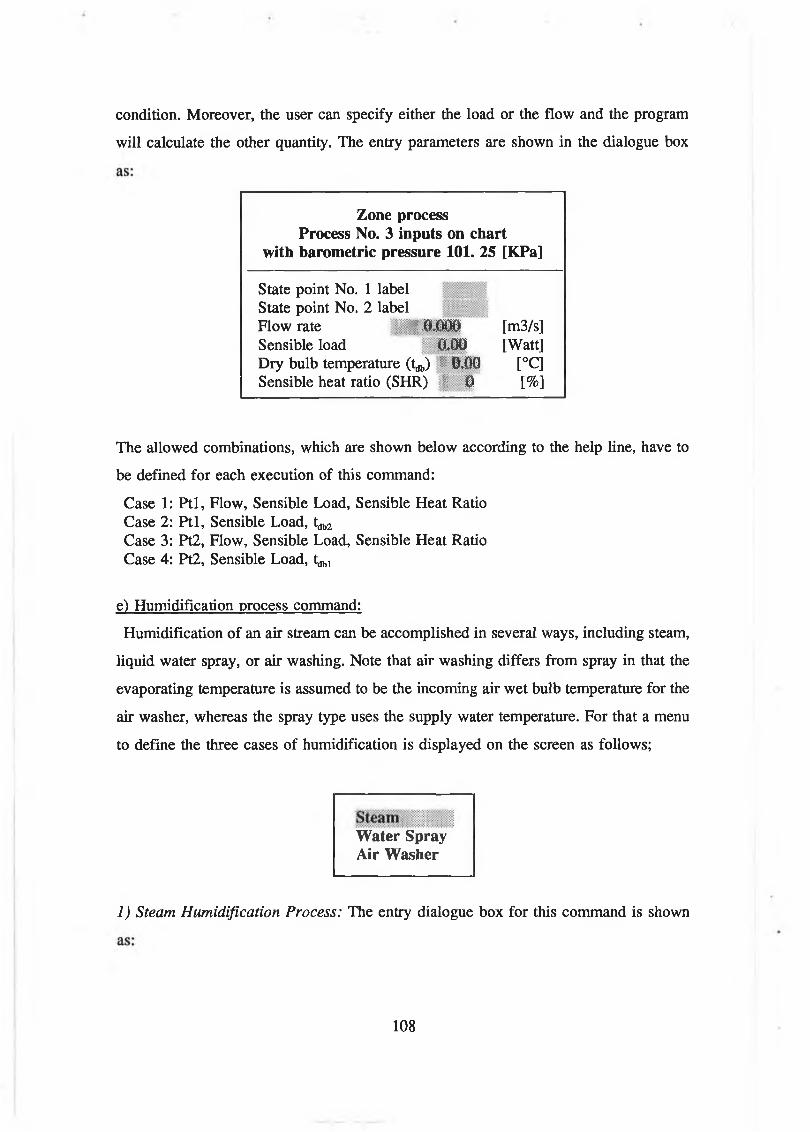
condition. Moreover, the user can specify either the load or the flow and the program
will calculate the other quantity. The entry parameters are shown in the dialogue box
Zone processProcess No. 3 inputs on chart
with barometric pressure 101. 25 [KPa]
State point No. 1 labelState point No. 2 labelFlow rate J | | -0.000 [m3/s]Sensible load 0.00 [Watt]Dry bulb temperature (tdb) ? 0,00 [°C]Sensible heat ratio (SHR) | 0 [%]
The allowed combinations, which are shown below according to the help line, have to
be defined for each execution of this command:
Case 1: P tl, Flow, Sensible Load, Sensible Heat Ratio Case 2: P tl, Sensible Load, tdb2 Case 3: Pt2, Flow, Sensible Load, Sensible Heat Ratio Case 4: Pt2, Sensible Load, tdbl
e) Humidification process command:
Humidification of an air stream can be accomplished in several ways, including steam,
liquid water spray, or air washing. Note that air washing differs from spray in that the
evaporating temperature is assumed to be the incoming air wet bulb temperature for the
air washer, whereas the spray type uses the supply water temperature. For that a menu
to define the three cases of humidification is displayed on the screen as follows;
Water Spray Air Washer
1 ) Steam Humidification Process: The entry dialogue box for this command is shown
108

Steam humidification process Process No. 5 inputs on chart
with barometric pressure 101. 25 [KPa]
State point No. 1 labelState point No. 2 labelFlow rate ' 0.000 [m3/s]Humidity ratio (W2) 0.00000 [Kg/Kg]Relative humidity (i>2) 0 [%]Steam enthalpy (1%) f l l l o [KJ/Kg]Steam temperature (X) / 0.00 [°C]
The allowed combinations, which are shown below according to the help line, have to
be defined for each execution of this command:
Case 1: P tl, Flow, <I>2, hs Case 2: P tl, Flow, 0 2, ts Case 3: P tl, Flow, W2, hs Case 4: P tl, Flow, W2, ts Case 5: Pt2, Flow, O l5 hs Case 6: Pt2, Flow, i>ls ts Case 7: Pt2, Flow, Wt, hs Case 8: Pt2, Flow, Wlt ts
2) Water Spray Humidification Process: The entry dialogue box for this command is
shown as follows and the allowed combinations are the same as the last case except the
enthalpy and temperature are for water instead of steam:
Water spray humidification process Process No. 6 inputs on chart
with barometric pressure 101. 25 [KPa]
State point No. 1 labelState point No. 2 labelFlow rate 0,000 |m3/s]Humidity ratio (W2) 0;00000 [kg/kg]Relative humidity (<I>2) 0 [%]Water enthalpy (hw) | 0.0()0 [kJ/kg]Water temperature ( t j 0,00 [°C]
3) Air Washer Humidification Process: The entry dialogue box for this command is
109

shown as follows and the allowed combinations are also as the last case:
Air Washer humidification process Process No. 7 inputs on chart
with barometric pressure 101. 25 [KPa]
State point No. 1 labelState point No. 2 labelFlow rate 0,000 [m3/s]Humidity ratio (W2) 0.00000 [kg/kg]Relative humidity (0 2) 0 [%]Water enthalpy (hw) 0.000 [kJ/kg]Water temperature (tw) 0 00 [°C]
f) Collecting process command:
The collecting process command is used when more than two streams are mixed
together, with known amounts and conditions for each stream. Physical examples would
include a conditioned space receiving air from several supply outlets, or a return plenum
collecting air from several zones. The program creates a collecting process by selecting
the command from processes menu, the number of stream which can be mixed are 2,3,4.
The allowed combinations are the flow rate and conditions (state point) for each stream,
the entry dialogue box for this command is displayed as:
Collecting process Process No. 8 inputs on chart
with barometric pressure 101. 25 [KPa]
State point No. 1 labelFlow rate of stream 1 0,000 [m3/s]State point No. 2 label P ill i liFlow rate of stream 2 0.000 [m3/s]State point No. 3 labelFlow rate of stream 3 0.000 [m3/s]State point No. 4 label iHow rate of stream 4 0.000 [m3/s]Collected state point No. M label Total Flow rate of stream M 0.000 [mVs]
110

g) Mixing Process command:
This command calculates the results of mixing two air streams. This command is
different from the other processes considered up to now in that it actually creates two
cases of mixing process:
• the one from the conditions of the first air stream to the mixed conditions
• the one from the conditions of the second air stream to the same mixed conditions
Mixing processProcess No. 7 inputs on chart
with barometric pressure 101. 25 [KPa]
State point No. 1 label ■
State point No. 2 label £'Total flow rate | | 0.000 [m/s]Percentage flow rate of Pt.2 | 0 [%]Mixed dry bulb temperature (tdb) 0.00 [°C]Mixed humidity ratio (Wm) 0.00000 [kg/kg]Mixed enthalpy (hm) 0.00 [kJ/kg]Mixed state point label
The allowed combinations, which are shown below according to the help line, have to
define for each execution of this command:
Case 1: P tl, Pt2, Total Flow, h2Case 2: P tl, Pt2, Total Flow, tdb2Case 3: P tl, Pt2, Total Flow, W2Case 4: P tl, Pt2, Total Flow, Percentage of Pt2
C h a r t S e t U p c o m m a n d :
This command is to define the limits of the psychrometric chart and the appearance
properties lines on drawing chart and calculations. The entry dialogue box for Chart
Setup is displayed on the screen as follows:
111
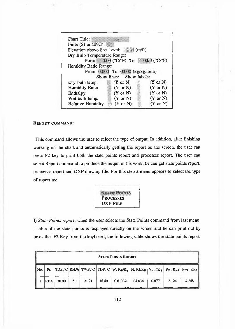
Chart Title: t i l l ■3Units (SI or ENG): § gElevation above See Level: 1 1 1 (m/ft)Dry Bulb Temperature Range:
Form 0.00 (°C/°F) To § 00 0 o’C/°F)Humidity Ratio Range:
TV» n r i ™ / Urr-lh/lVO
Show lines: Show labels:Dry bulb temp. (Y or N) gf (Y or N)Humidity Ratio (Y or N) (Y or N)Enthalpy (Y or N) (Y or N)Wet bulb temp. (Y or N) (Y or N)Relative Humidity | | (Y or N) (Y or N)
R e p o r t c o m m a n d :
This command allows the user to select the type of output. In addition, after finishing
working on the chart and automatically getting the report on the screen, the user can
press F2 key to print both the state points report and processes report. The user can
select Report command to produce the output of his work, he can get state points report,
processes report and DXF drawing file. For this step a menu appears to select the type
of report as:
State Points P r o c e s s e s D X F F i l e
I) State Points report: when the user selects the State Points command from last menu,
a table of the state points is displayed directly on the screen and he can print out by
press the F2 Key from the keyboard, the following table shows the state points report
Sta t e P o in ts R e p o r t
No. Pt. TDB,°C RH,% TWB,°C t d p ,°c W, Kg/Kg H, KJ/Kg V,m3/Kg Pw, Kpa Pws, KPa
1 REA 30.00 50 21.71 18.40 0.01332 64.034 0.877 2.124 4.248
112

II) Processes report: Any execution for this command give the user processes report on
the screen, and also he can get printout this report by press F2 key which is printed as
shown in the following table:
P r o c e s s e s r e p o r t
No.Proc.Type
FromPt.
ToPt.
Rowm3/Kg
Sensible Load KJ/Kg
Latent Load KJ/Kg
WateraddedKg/hr
TotalLoad
KJ/Kg
HI) DXF File (Drawing File): This command allows the user to get DXF file on disk
that can be read by the AutoCAD package. This feature allows the user to incorporate
psychrmetric chart graphical results into reports and drawings. All DXF files are written
in the directory established by the AutoCAD directly (i.e. C:\ACAD\). To use the DXF
files the user has to execute the AutoCAD package if he was only executing HVACS YS
package or if he executed the HVACSYS within the AutoCAD, he has to exit from the
HVACSYS package. After that he can call the DXF file by using DXFIN command
from AutoCAD and type the file name. Fig.(3.21) shows a psychrometric chart for sea
level drawn using DXF file.
3.6 U-VALUE PROGRAM:
The calculation of HVAC loads begin with the determination of U-value, which are
overall heat transfer coefficients. U-value are calculated by taking the reciprocal of an
R-value (net effective heat transfer resistance). R-value is obtained by dividing the
thickness of the material layer by the conductivity of the material used for common
building, and these are listed in tables in the Appendix. This program calculates the
thermal transmittance or U-value of a structure which may be a wall, roof or floor . In
this program the master menu is divided into seven submenus as seen in the flowchart
in Fig.(3.22).
The type of surface ( eg. outside w all) will define the internal surface resistance. Each
normal solid layer has a defined thickness and thermal conductivity, and so on for the
113

Fig. (3.22) Flow Diagram of The U-Value Programme Procedures

( ^ S t a r t S u b ^ )
1. Air Gab2. Asbes tos3. As ph a l t4. Blocks5. Br ick6. Clay & Soil7. Con cr e t e8. Fel t9. F l o or in g
10. Gene r a l Concre te11. I n s u l a t i o n12. Maso nr y13. Metals14. M i n e r a l I n s u l a t i o n15. M i s c e l l a n e o u s16. P l a s t e r17. R o of i n g C omp onen t s18. S h ee t i n g19. T imb er20. Vapour Bar r i e r s
n = n + 1 Material C lasses Menu
Select Material for \ ( i )
»j Layer Length L(i) j i = i + l
Fig. (3.23) Flow Diagram o f The Layer Resistance Subroutine
115

next layer until the construction of the surface is completed. Up to 20 layers may be
specified. Air gaps are not counted as layers, but specified separately. Fraction of air
gaps may be used if a non standard thermal resistance is required.
3.5.1 U-VALUE PROGRAM EXECUTION STEPS:
The overall structure of U-value program is given in Fig.(3.22) which is explained the
sequences of the running procedure of the program. And Fig.(3.23) shows the main
subroutine of the U-value program.
U-Value Submenu:
Any selection of U-value function from submenus gets the user through the U-value
program. The following menu called "The surfaces types menu" appears to select the
appropriate surface to work on. This menu consists of seven options, as follows:
External Wall External Flat Roof Pitched Roof Internal Wall Internal Roof Solid Ground Floor Basment
The user selects the option required to continue the program to the next step.
External Surfaces :
The external surfaces contain the external wall, external roof, and the pitched roof. The
CIBSE GUIDE [2] gives the following specifications for the external surfaces;
* Sheltered is up to the third floor height in city centres.
* Normal comprises most suburban and country premises; fourth to eighth floors in
116

city centres.
* Severe comprises buildings on the coast or exposed hill sites, floors above the fifth
in suburban or country districts; ninth and above in city centres.
Then for these definition a site exposure menu is displayed on the screen as follows:
Shelter*!!!NormalSevereSpecial
The site exposure menu helps to define the external surface resistances according to
Table (3.11).
Wall Internal floor Flat
Heat Up Heat down roof
R* 0.123 0.106 0.15 0.106
Ra 0.18 0.18 0.21 0.18
Sheltered 0.08 0.106 0.15 0.07
Rso Normal 0.05 0.106 0.15 0.045
Severe 0.03 0.106 0.16 0.02
Table 3.11 Outside, inside, and air gab thermal resistances
For example the Sheltered option gives for the out side thermal resistance 0.08 m2oC/W
for the Wall and 0.07 m2oC/W for the roof and Roof-part in pitched roof and so on for
other options. In addition to that if the user chooses special option, it gives a choice to
enter the value of special thermal resistance ( R^, R^ ).
The general equation (3.6.1) for a layered external wall, external roof, and external
117
I

floor is :
t/= -1
* / E y * « V * .i
(3.6.1)
i=l
Where:
U = Thermal transmittance ( W / m2oC ).
Rsi = Inside surface resistance ( m2oC / W ).
Rs0 = Outside surface resistance ( m2oC / W ).
Ra = Air gap resistance ( m2oC / W ).
n = Number of air gaps.
Lj = Thickness of layer i ( m ).
= Thermal conductivity of layer i ( W / m2oC ).
m = Number of solid layers.
Pitched Roof:
For pitched roofs the structure is considered in two parts, firstly the ceiling construction
and than the roof. Individual U values are computed for both elements using internal
surface resistances for the ceiling giving a U value as U1 by using equation (3.6.2) with
only a little change in equation (3.6.1) to become :
t/=-1
2 «* E x * « 8.J=1
(3.6.2)
And one internal and one external surface resistance for the roof giving a U value as
U2 by using equation (3.6.1). The resulting combined U-value (equation (3.6.3)) is
computed using the pitch angle (a) as :
118
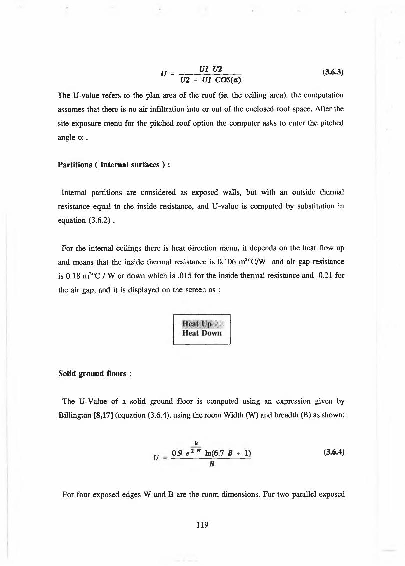
u = UJ_U2 (3.6.3)U2 + U1 COS(a)
The U-value refers to the plan area of the roof (ie. the ceiling area), the computation
assumes that there is no air infiltration into or out of the enclosed roof space. After the
site exposure menu for the pitched roof option the computer asks to enter the pitched
angle a .
Partitions ( Internal surfaces ) :
Internal partitions are considered as exposed walls, but with an outside thermal
resistance equal to the inside resistance, and U-value is computed by substitution in
equation (3.6.2) .
For the internal ceilings there is heat direction menu, it depends on the heat flow up
and means that the inside thermal resistance is 0.106 m2oC/W and air gap resistance
is 0.18 m2oC / W or down which is .015 for the inside thermal resistance and 0.21 for
the air gap, and it is displayed on the screen as :
Solid ground floors :
The U-Value of a solid ground floor is computed using an expression given by
Billington [8,17] (equation (3.6.4), using the room Width (W) and breadth (B) as shown:
E
v _ 0.9 e 2w ln(6.7 B + I) (3.6.4)B
For four exposed edges W and B are the room dimensions. For two parallel exposed
119
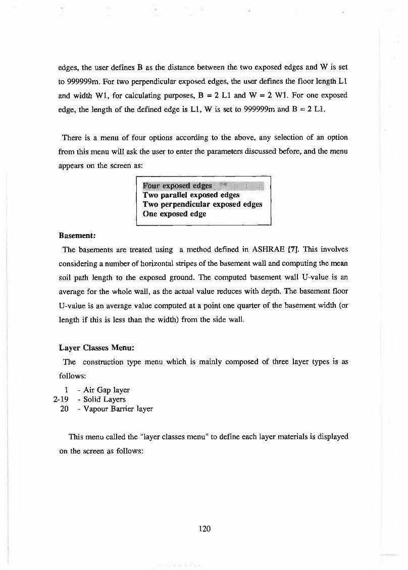
edges, the user defines B as the distance between the two exposed edges and W is set
to 999999m. For two perpendicular exposed edges, the user defines the floor length LI
and width W l, for calculating purposes, B = 2 LI and W = 2 W l. For one exposed
edge, the length of the defined edge is LI, W is set to 999999m and B = 2 LI.
There is a menu of four options according to the above, any selection of an option
from this menu will ask the user to enter the parameters discussed before, and the menu
appears on the screen as:
Four exposed edges Two parallel exposed edges Two perpendicular exposed edges One exposed edge
Basement:
The basements are treated using a method defined in ASHRAE [7]. This involves
considering a number of horizontal stripes of the basement wall and computing the mean
soil path length to the exposed ground. The computed basement wall U-value is an
average for the whole wall, as the actual value reduces with depth. The basement floor
U-value is an average value computed at a point one quarter of the basement width (or
length if this is less than the width) from the side wall.
Layer Classes Menu:
The construction type menu which is mainly composed of three layer types is as
follows:
1 - Air Gap layer2-19 - Solid Layers
20 - Vapour Barrier layer
This menu called the "layer classes menu" to define each layer materials is displayed
on the screen as follows:
120
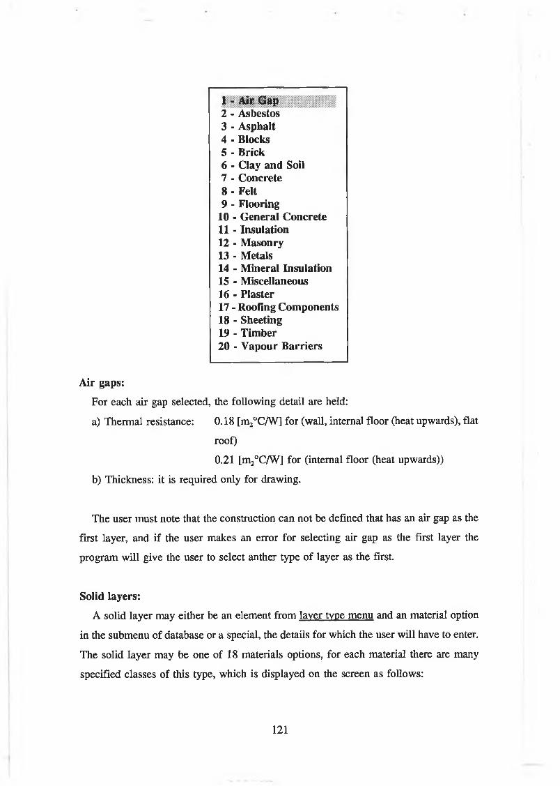
1 - Air Gap2 - Asbestos3 - Asphalt4 - Blocks5 - Brick6 - Clay and Soil7 - Concrete8 - Felt9 - Flooring
10 - General Concrete11 - Insulation12 - Masonry13 - Metals14 - Mineral Insulation15 - Miscellaneous16 - Plaster17 - Roofing Components18 - Sheeting19 - Timber20 - Vapour Barriers
Air gaps:
For each air gap selected, the following detail are held:
a) Thermal resistance: 0.18 [m2°C/W] for (wall, internal floor (heat upwards), flat
roof)
0.21 [m2°C/W] for (internal floor (heat upwards))
b) Thickness: it is required only for drawing.
The user must note that the construction can not be defined that has an air gap as the
first layer, and if the user makes an error for selecting air gap as the first layer the
program will give the user to select anther type of layer as the first.
Solid layers:
A solid layer may either be an element from layer type menu and an material option
in the submenu of database or a special, the details for which the user will have to enter.
The solid layer may be one of 18 materials options, for each material there are many
specified classes of this type, which is displayed on the screen as follows:
121

Table (3.12) Asbestos Material for U-Value Calculation.
ASBESTOSThermal dens Spce. Vapor
No. Description Cond. ity heat R e s .W/m °C Kg/m3 J/Kg°C GNs/Kgm
1 Asbestos 83% magnesia 0 .070 190 1000 300.002 Asbestos cement decking 0 .360 1500 1050 300.003 Asbestos cement sheet 0.360 700 1050 300.004 Asbestos slabs 0.070 145 1000 300.005 Asbestos sprayed (80 kg/m3) 0.043 80 816 1000.006 Asbestos sprayed (13 0 kg/m3) 0.046 13 0 816 1000.007 Asbestos sprayed (160 kg/m3) 0.061 160 816 1000.008 Asbestos sprayed (240 kg/m3) 0.068 240 816 1000.009 Asb cement sheet (700 kg/m3) 0 .360 700 1050 333.33
10 Asb cement sheet (13 60 kg/m3) 0 .220 1360 1050 333.3311 Asb cement sheet (1520 kg/m3) 0 .360 1520 1050 333 .3312 Asb cement sheet (1600 kg/m3) 0 .400 1600 1050 333 .3313 Asb cement sheet (2000 kg/m3) 0 .660 2000 1050 333 .3314 Asbestos cement board (type 1) 0 .577 1922 1005 333 .3315 Asbestos cement board (type 2) 0.389 1970 837 333 .3316 Asbestos cement 0 .360 750 2133 1000.0017 Asb cement, semi compressed 0.370 1200 2133 1000.0018 Asb cement, fully compressed 0.650 1600 2133 1000.0019 Asb insul board (500 kg/m3) 0.108 500 840 333 .3320 Asb insul board (577 kg/m3) 0.160 577 840 333 .3321 Asb insul board (720 kg/m3) 0.120 720 840 333 .3322 Asb insul board (900 kg/m3) 0.115 900 840 333 .3323 Asb insul board (12 00 kg/m3) 0 .250 1200 840 333.3324 Asbestos cement new 0 .360 750 2133 1000.0025 Asbestos cement aged 0 .360 750 2133 1000.0026 Asbestos cement, red 0 .360 750 2133 1000.0027 Asbestos fibre loose 0.061 12 8 816 333 .33
Layers are defined starting from the inside outwards and each layer may be one of
three types as defined. Each type of the material in this menu has a list of different
types from these materials as shown in appendix A, Tables 1-16. For example if one
selects Blocks option from the menu the material will list into pages and one can select
from any page and if the first page is missed it may be displayed again by following the
command appearing on the screen. After this stage the user has to define the thickness
of each layer and so on for the next layer till finishing the structure.
For building up standard files for the users own material he can refer to materials
option in the submenu of database. In addition, for each of the three groups of materials
the user may define a special material, easily to select the type of layer, and for this
layer there is a materials menu to choose the layer material.
The result of U-value may be displayed or saved to be used when it is needed.
122
I

CHAPTER FOUR
CUSTOMIZING CAD SYSTEMS FOR HVAC SYSTEMS
DESIGN
4.1 INTRODUCTION:
With the advent of high speed Computers, Computer-Aided Drafting (CAD)
system have become omnipresent among design engineers. From the initially very
expensive system, with simple interactive geometric capabilities, CAD system have
evolved into affordable but sophisticated tools that automate many aspects of design
documentation and retrieval. The development of even routine designs, however, has
still been a manual (and often tedious) process. These first generations CAD tools have
provided gains in drafting productivity of 50% to 200% [30] in repetitive design
applications.
This chapter describes the evolution of a new kind of knowledge-based CAD
system, HVACCAD. HVACCAD is a computer-supported engineering consulting tool
and leading software package for the user in designing the pipe and duct systems. It is
based on AutoCAD which is one of the world’s leading CAD and graphics program.
By providing significant new capabilities to support both the development and
documentation of design solutions, HVACCAD increases productivity in design
projects by 10 to 15 times, freeing engineers to make fuller use of this skills and
creativity. HVACCAD Allows storage and re-use of engineering knowledge, supports
engineering teamwork and concurrent engineering, integrates engineering disciplines,
and automates generation of documents, including drawing parts list, parts prices, total
costs and specifications.
In a HVAC design the individual environmental plant components are connected
to other components by pipes, ducts and control systems to form a complete system.
123
i

An engineer’s schematic diagram may be represented by a network of "Nodes" and
"arcs", the nodes representing components such as fans, boiler, burners, pumps, AHU,
U H ..., and the arcs representing the inter connecting pipes and ducts and their fittings.
The concept of developing CAD for drawing HVAC System networks, has been
interpreted in a number of different ways by other researchers [37-52]. Thus the user
has mainly two systems for further design development;
1) duct system
2) pipe system and
both these systems are appropriate for the HVAC system design. Each system has its
own nodes and arcs, for example for duct work; AHU, dampers, filters, supply outlets,
grills, coils, fans is deceived as nodes and the duct and its fitting like elbows, tees,
reducers as arcs.
In addition to these subroutines, psychrometric chart program has been
developed for any elevation to represent all HVAC Process. It is a complete chart for
temperature range -50 to 100 °C, and humidity ratio 0 to 0.35 kgw/kga.
4.2 HVACCAD USER INTERFACE:
The menu file in AutoCAD package is a simple text file containing AutoCAD
command strings (ACAD.MNU file). Section of the file can be associated with different
menu device, such as the screen and tablet menus. Both pull-down and screen menus
have been used in this work. The command HVACCAD is added to the main menu,
this command calls the HVACCAD user interface where a special menu file called
HVAC.MNU is developed similar to ACAD.MNU which have been customized as
menu for HVAC system design, and activates several submenus which invoke the
developed routines.
The user interface is accomplished by integrating HVACCAD which is present
as customized AutoCAD and relational DATABase which is calculated or stored by
HVACSYS using ASCII files between them. In the product structure rooms, spaces and
components o f HVAC system are visualized as a logical hierarchy with depending
124

HVACCAD M a i n M e nu Us er I n t e r f a ceI
D A TA Base C o m p o n e n t s & E q u i p m e n t |^Z
S e l e c t i o n & Pr ice s
HVACCADS u b m e n u s Ì
HVAC System D r a w i n g P lans &
R e p o r t s p r i n t o u t
HVACCAD Bar Menu HVACCAD Screen Menu
P i p e
Access o r i e s
V a l v e
H a n g e r s
e t c .
B o i l e r s
B u r n e r s
Pumps
R a d i a t o r s
U . H e a t e r s
e t c .
D u c t
A c c e s s o r i e s
AHU
's
F a n s
D a m p e r s
H a n g e r s
e t c .
G r i l l s
C o i l s
H u m i d i f i e r s
Ico n M enus
HVACCAD«jç «jç ^ <j «jg
D u c t w o r k
Pi pewo rk
P s y c h a r t
Pr i n tPl ot
HVACSYS
AutoCAD
Fig (4.1) hierarchy o f the HVACCAD package structure
— R e c t a n g u l a r -----
— R o u n d -----
_ F l e x i b l e -----
__ S u p p l y u p ___ S u p p l y d o w n
„ E x h a u s t op
_ E x h a o s t d o w n
-----
D u e l — ------
• R a d i o s B e n d s
■ M i t r e b e a d s
S h o e b r a n c h
A n g l e d B r a n c h
’ B e l l m o n t h B r a n c h
. E x p a n s i o n & ____ A H UC o n t r a c t i o n
* F l e x i b l e C o n n e c t i o etc.
- E q u i p r o e n t
" HVACCAD_ _ H o r i z o n t a l
V e r t i c a l <\— G e n e r a l
P i p e -----1
. F l o w Up
F I o w D o w n
- P i p e
* A c c e s s o r i e s
- V a l v e s --------
- H a n g e r s
- E q u i p m e n t
- HVACCAD
P i n gC h e c k — ==: M o t o r i z e d « e t c .
S t a t e p o i n t
, P r o c e s s —
, W i n d o w
, HVACCAD
, G e n e r a l
■ Heating■ C o o l i n g
■ H u m i d i f i c a
■ Z o n e
. M i x i n g
C o l l e c t i n g
■ T D B A R H
. T D B & T W B
■ T D B & T D P
■ T D B & W
. T D B & H
. R H & T W B
■ R H & T D P
. R H & W
- R H & H
► T W B & T D P
- TWB&W
. T D P & H
W& H
P u
- R a d i a t o r s 4
- U . H e a t c r s <
. F a n C o i l s ^
. e t c .
S c r e e nM e n u s
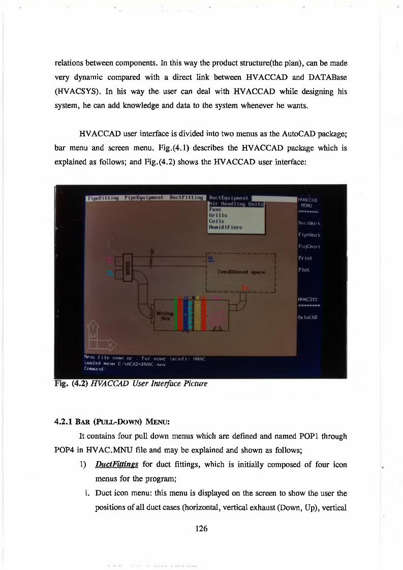
relations between components. In this way the product structure(the plan), can be made
very dynamic compared with a direct link between HVACCAD and DATABase
(HVACSYS). In his way the user can deal with HVACCAD while designing his
system, he can add knowledge and data to the system whenever he wants.
HVACCAD user interface is divided into two menus as the AutoCAD package;
bar menu and screen menu. Fig.(4.1) describes the HVACCAD package which is
explained as follows; and Fig.(4.2) shows the HVACCAD user interface:
HWtCCADHENU
ftictUork
Pi[icUarfc
PxijChiirt
tfUftCSYS
rluloCftD
M ou f l i c nane o r f o r none <acad>: ItUflC Loaded neroi C :\ftCAD\iW flC.nnx Cwwand :
Fig. (4.2) HVACCAD User Interface Picture
4.2.1 B ar (Puli -Do w n ) M enu:It contains four pull down menus which are defined and named POP1 through
POP4 in HVAC.MNU file and may be explained and shown as follows;
1) DuctFittines for duct fittings, which is initially composed of four icon
menus for the program;
i. Duct icon menu: this menu is displayed on the screen to show the user the
positions of all duct cases (horizontal, vertical exhaust (Down, Up), vertical
126

supply (Down, Up)). A sample of this menu can be designed and displayed
as following:
rtenu M l e n a n e o r . T o r n o n e < a c m l> : n u n c Loaded ncmi C : srtCODvHUAC .mix C(nhm nd:
Fig. (4.3) Duct Icon Menu Picture
ii. Accessories icon menu: the most important in the duct network is the fitting
of the duct like elbows with deferent type, tees, wyes, reducers, diffuser,
etc. Fig. (4.4) shows a picture of some of the duct fitting.
iii. Dampers icon menu; the dampers for the duct system are important to
control the air distribution and balance the system. The dampers can be
classified through: butterfly, multiblade (parallel-blade, opposing-blade),
motorizing and manual, fire and smoke controls damper, splitter, gate or
slide and shutter.
iv. Filters icon menu: air filter can be classified as:
1) Fibrous filters which have four general configurations (panel filters,
pleated-medium filters, tubular packed or bag filters and roll filters).
2) Membrane filters: membrane filters are made from very thin polymer
sheets pieced by extremely small air-flow passages, these are available in
127

several forms (collimated pore, granular symmetric, granular asymmetric,
fibre).
3) Electrostatic filters.
4) Combined forms.
2) DuctEquip for Duct equipment, Which is composed of five commands:
i. Air Handling Unit (AHU) icon menu: The function of the AHU is to
provide air at a quantity, temperature and humidity to offset the sensible
and latent heat gains to the space (in the cooling mode) and the heat losses
(in the heating mode), while maintaining the required temperature and
humidity in the space. AHU can be classified on its arrangements as: (a)
single zone, (b) multizone, (c) double duct, (d) variable air volume (VAV)
and (e) induction.
ii. Fans icon menu: This menu contains all type of fans which can be
classified as follows and Fig.(4.5) shows a number of types of fans which
can be used:
1. Axial flow fan, including propeller fans, through which the air
flows substantially parallel to the shaft.
2. Centrifugal fans, which might be called radial-flow fans
because the air flows in a radial direction relative to the shaft.
3. Mixed-flow fans, through which the air flows in a combined
axial and a radial directions.
4. Cross-flow fans, through which the air flows in an inward
radial direction and then in an outward radial direction.
iii. Diffuser and Grill icon menu: A diffuser is an outlet through which the air
supply passes from the duct system to the space being conditioned which
can be classified as (multiple strip ceiling diffusers, cone-type ceiling
diffusers, perforated-face ceiling diffusers, multi-directional ceiling
diffusers, linear ceiling diffusers, side wall diffusers, etc.). A grille is
defined as a covering for an opening through which air passes (extract or
return air
128

Fig. (4.4) D uct Fittings Icon Menu Picture
ductuorkHEMU
Fig. (4.5) Fans Icon Menu Picture
129

grilles);. A register is a grille with a damper for volume control. While
these are the technically correct definition, common usage refers to supply
outlets in walls and floors as grilles or registers, and to ceiling outlets as
diffusers.
iv. Coils icon menu: The coils for cooling and heating can be classified
through which the working fluid passes: water coils (hot and cold), direct
expansion coils (DX), steam coils and according to the arrangement of
rows, tubes, circuits and according to fins type (aluminum, cooper, steel,
copper-nickel, or stainless steel) and their arrangements (continuous plate
fins, flat, corrugated, or louvred).
v. Humidifiers icon menu: According to the type of humidification there are
three types of humidifiers (steam humidifiers, spray water humidifier and
air washer humidifiers) .
3) Pipefittine for pipe fittings,
i. Pipe icon menu: This menu contains all types of pipes according to the kind
of metal and the insulation according to the pipe place. It can be displayed
as shown in Fig.(4.6) with five types of pipes (painted steel pipe, inside
insulated steel pipe, outside insulated steel pipe, copper pipe and insulated
copper pipe).
ii. Accessories icon menu: The major piping materials are produced in the
form of standard fittings. Among the more widely used materials are cast-
iron, malleable-iron, brass, copper, cast-steel and wrought-steel. Cast-iron
fitting might be in three types (threaded, bell-and-spigot, flanged), and cast
steel fitting might be flanged and welded, copper might be threaded and
welded. Fig. (4.7) shows some types of pipe fittings which are elbows, tees,
concentric, eccentric, wyes, caps, crosses, etc.
iii. Valves icon menu: The valves can be classified in two types (threaded and
flanged, and according to their uses which are gate valve, globe valve, ball
valve, butterfly valve, check valve (spring, swing), safety relief valve,
solenoid valve, three way valve (motorized, manual). Fig.(4.7) and
Fig.(5.8) show some of these valves.
iv. Hangers icon menu: Pipe specifications for individual projects must be
130
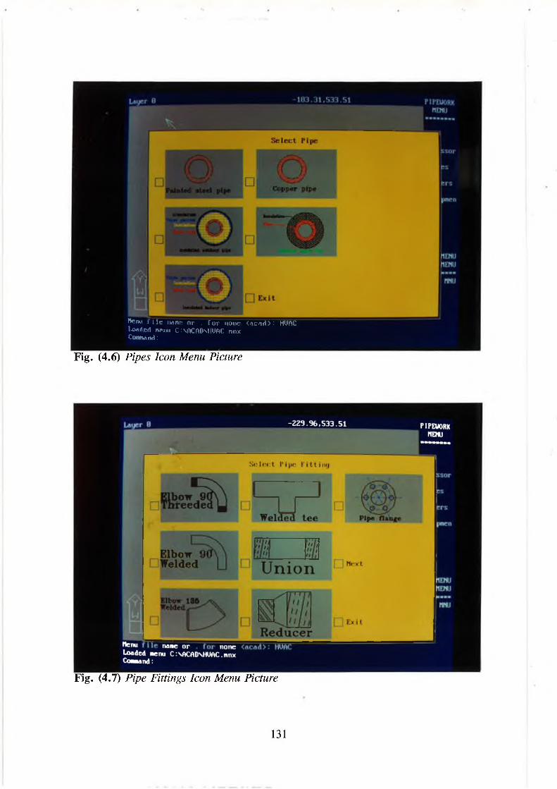
ncm ' r t i e n a n e o p . f o r n o n e < ac*d> : HUfiC Loaded ncitu C:\ftCflO\HUftC.nnx C o M M n d :
Fig. (4.6) Pipes Icon Menu Picture
Fig. (4.7) Pipe Fittings Icon Menu Picture
131

written in such a way as to assure proper support under all operating and
environmental conditions and to provide for slope, expansion, anchorage, and
insulation protection, then they are mainly classified as supports, anchors,
restraints and guides.
4) PiveEquio for pipe equipment,
i. Boilers icon menu: While many types of boilers are manufactured today
which differ in size, configuration, materials, and construction methods, the
popular types are firetube (usually for hot water), watertube for steam (D-
style, A-style), and cast-iron sectional boilers (internal push nipples,
external headers). These can also be classified on the type of fuel (gas, oil,
solid like Firebox boilers).
ii. Burners icon menu: according to the boiler type and the capacity, the
burners and the type of fuel can be classified as follows:
a. Gas burners.
b. Oil burners.
c. solid fuel burners.
iii. Pumps icon menu: Pumps can be classified into two basic types; centrifugal
(frame-mounted and close-coupled end-suction pumps, double suction
centrifugal pumps, vertical multistage pumps, horizontal multistage pumps,
submersible pumps, self-priming pumps, axial-flow pumps and regenerative
pumps), and positive displacement (reciprocating pumps, power pumps,
steam pumps, rotary pumps( sliding-vane, gear). For heating and cooling
systems mainly centrifugal pumps are used specially the first one with
multi-shapes (inline pump, dual inline pump, base mounted pump, etc.).
iv. Radiators icon menu: radiators can be classified according to the metal
which is made from as follows; cast iron sectional radiators (open front to
section, section extended at front), steal radiators (simple convoluted panel
(single, double or more), column type like cast-iron radiators, a sinuous
coil panel type, tubular type, etc.). Aluminium radiators are the same as
cast-iron radiators and may be used as convector, cabinet convectors (flat-
top front outlet, slope-top enclosure, flat-top top outlet, etc.).
v. Unit Heaters icon menu: Unit heaters can be classified as follows:
132

• By type of air mover: (either propeller or centrifugal blower).
• By physical configuration: (either Vertical or Horizontal air delivery).
• By heating medium: (Steam, hot water, gas, oil, or electricity).
4 . 2 . 2 S c r e e n M e n u :
This is composed of five commands;
1 ) Ductwork command:
I. Duct command: For this command the user meet three kind of duct that
may be found in duct design:
a. Rectangular duct.
b. Round duct.
c. Flexible duct.
Each of these kinds may have two positions in the drawing
therefore there are two commands to cover these: horizontal and vertical.
For vertical, there are two types, supply and exhaust. For the supply and
exhaust duct there are also two commands to define the direction of flow
Up or Down.
II. Accessories command: For duct accessories like elbows, junctions (tees,
wyes, crosses), transitions, etc.
III. Dampers command;
IV. Hangers command;
V. Equipment command: To cover all ductwork equipment like AHU, VHU,
diffusers, fans, coils, filters, humidifiers, etc.
VI. HVACCAD command: To let the user to go back to the main HVACCAD
menu. This command will be repeated in each submenu.
VII. AutoCAD command: To let the user to go back to the main AutoCAD
menu. This command is repeated in each submenu.
2 ) Pipework command:
I. Pipe command: For this command the user meets three positions of pipe
that may be found in pipe design:
a. Horizontal pipe.
134

b. Vertical pipe; for this option there are two kinds (flow up and down),
c. General pipe.
II. Accessories command: For pipe accessories like elbows, junctions (tees,
wyes, crosses), transitions, etc.
III. valves command:
IV. Hangers command:
VI. Equipment command: To cover all pipework equipment like Boilers,
Burners, Pumps, Radiator, Unit heaters, Fan coils, etc.
3 ) PsyChart command:
I. State point command: For this command the user meets 13 commands
according to the allowable combinations of the input parameters.
II. Process command: To cover all processes of air conditioning on the
psychrometric chart.
III. Window command:
4 . 3 P I P E S I Z E C A L C U L A T I O N P R O G R A M :
This program is an AutoCAD-based piping system design layout and drafting
program; it uses the AutoCAD pull-down and ICON menus fully. Drawing initialisation
is handled by a start-up macro which automatically controls the placement of the
drawing border, "North Arrow", and even sets up boundary limits. Furthermore, the
direction of the "North Arrow" has intelligence and its information is used to adjust the
User Coordinate System (UCS) accordingly.
PIPEWORK also offers the end user the ability to customise most aspects of the
program. The default drawing borders can be replaced with the user’s own or with a
client’s border instead; the user just needs to copy the prototype drawing border as
biking up border subroutine and select the user window in the proper directory and it
can be used with PIPEWORK.
The program can also be configured to work with either imperial, metric or
135

mixed metric units. After selecting the drawing size, the software automatically sets up
the appropriate distance units.
The best feature of PIPEWORK is its specification-driven interface. All new
pipes are assigned to the current pipe specification, such as 150 carbon steel or PN16
Stainless and the current ‘spec’ can be changed at any time. These specifications are
maintained in the same external database common to all the PIPEWORK piping
programs, so that there is only one ‘spec’ being used to create P&IDs, Isometrics and
3D models. This database is completely user definable and supports ANSI, DIN and
other common standard components.
PIPEWORK can be used as either a 2D or 3D system and the user can work in
any view. However, one may find it easier to work with two simultaneous view ports:
top and iso. Pipe centre line is routed in a plan view and insert fittings in one of the
four isometric views. The layer facility is used to place each piece of equipment on a
separate layer and then grouped pipes by either system to allow better visualisation of
a high-density model.
The software employs what appears to be a unique system architecture. All non
graphic attribute information is stored in an external, DATABase files. This seems to
reduce the size of the AutoCAD *.DWG file and makes all the material information
accessible for reporting, estimating and general material control applications.
Each graphic instant of a valve or fitting is linked, via AutoCAD’s handles, to
a record in the external DATABase. Some of the dimensional data, such as length or
weight, is automatically extracted from the pipe specification. Other information, such
as name or mark number, is user assigned at installation. PIPEWORK comes with user
customizable forms for each type of component-valves, flanges, fittings, pipe, etc. The
database file can also be modified to store the cost or expediting information. This is
done so it can become the basis of other configuration management solutions.
Many CAD programs enable the user to lay out piping. However, one of
136

PIPEWORK’s strongest features is its pipe-editing function. The external database files
makes it easy to delete items; no hunting for invisible attribute blocks inserted
somewhere in the drawing. Unlike other programs, this one uses the actual pipe line
lengths, not attributes, to determine bill of material values. The actual cut length is
adjusted by the system to account for threaded or socket-weld engagements and weld
gaps. This means the user can use all standard AutoCAD-editing commands, such as
STRETCH and MOVE, to adjust piping configurations.
PIPEWORK uses a centre line based routing system and, while they take some
getting used to, there are some good tools to perform fitting make-up operations at
elbows and tees. A "change length" and "replace pipe" command also assists in making
changes to existing pipe runs.
No system is worthwhile unless it can produce standard plan and section
drawings PIPEWORK enable the user to create either. Double-line representations of
the piping can be created such as is suitable for orthographic drawings
This double-line representation is created on a separate layer called 2-D and a
switch enables the user to limit the double line generation to a given pipe size and
above. With this, the user can conform to the industry practice of showing small bores
in single line. Users have access to all AutoCAD commands for 2D cross-hatching of
platforms and detailing of handrails, etc. Standard AutoCAD dimensioning commands
are used within the software to present the actual lengths and diameters of pipe runs and
equipment. Another important feature of HVACCAD is its ability to make automatic
sections. Also, standard details from several parts of the model can be inserted into a
separate drawing. This could be useful for exploded views of complex areas.
4 . 3 . 1 P ip e s iz in g t h e o r e t ic a l a n a l y s is :
Before any part of the water piping system can be sized, the probable rate of
flow in any particular section of piping should be determined. The rate of flow in the
service line, risers, and main branches. The formula which can be applied to get the
137
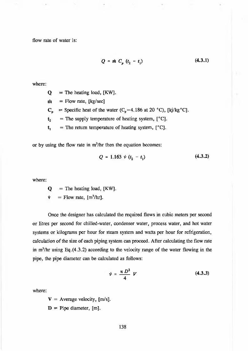
where:
Q = The heating load, [KW].
m = Flow rate, [kg/sec]
Cp = Specific heat of the water (Cp=4.186 at 20 °C), [kj/kg°C].
t2 = The supply temperature of heating system, [°C].
t, = The return temperature of heating system, [°C].
or by using the flow rate in m3/hr then the equation becomes:
Q = 1.163 v (f2 - t j (4.3.2)
flow rate of water is:
Q = m Cp (t2 - fj) (4.3.1)
where:
Q = The heating load, [KW].
v = Flow rate, [m3/hr].
Once the designer has calculated the required flows in cubic meters per second
or litres per second for chilled-water, condenser water, process water, and hot water
systems or kilograms per hour for steam system and watts per hour for refrigeration,
calculation of the size of each piping system can proceed. After calculating the flow rate
in m3/hr using Eq.(4.3.2) according to the velocity range of the water flowing in the
pipe, the pipe diameter can be calculated as follows:
v = J L ® ! y ( 4 . 3 . 3 )4
where:
V = Average velocity, [m/s].
D = Pipe diameter, [m].
138

From the pressure drop caused by fluid friction, in fully developed flows of all
"well behaved" (Newtonian) fluids, is described by Darcy-Weisbach equation:
(4.3.4)
where:
AP = Pressure drop, [Pa].
/ = Friction factor, dimensionless.
L = Length of pipe, [m].
p = Fluid density at mean temperature, [Kg/m3].
This equation is often presented in head or specific energy form as:
where:
Ah = Head loss, [m].
g = Acceleration of gravity, [m/s2].
In this form, the density of the fluid does not appear explicitly (although it is in
the Reynolds number, which influences/). The friction facto r/is a function of the pipe
roughness e, inside diameter D, and a dimensionless parameter, Reynolds number:
(4.3.5)
(4.3.6)v
where:
v = Kinematic viscosity of the fluid, [m2/s].
139

The friction factor is frequently presented on a Moody chart, giving a function
of Re with e/D as a parameter. A useful fit of smooth and rough pipe data for the usual
turbulent flow regime is the Colebrook equation:
— = 1.74 - 2 log — + I f Di f
2 e + 18.7
D + ^ i f
(4.3.7)
where:
e = absolute roughness of the pipe wall, [m].
The equation is implicit in / , / appears on both sides, so that a value for / is
usually obtained iteratively. A less widely used alternative to Darcy-Weisbach
formulation for calculating pressure drop is the Hazen-Williams equation, expressed as:
where:
C = Roughness factor.
Recommended values of C are 150 for plastic pipe and copper tubing, 140 for
new steel pipe, down to 100 for below and badly corroded or very rough pipe.
Valve and Fitting losses:
Valves and fittings cause pressure losses greater than those caused by the pipe
alone. One formulation expresses losses as:
(4.3.8)
or
(4.3.9)
or
140

(4.3.10)
V1A h = k —
2 g(4.3.11)
where:
k = Geometry and size dependent loss coefficient, Table (1, 2, 3) in
Chapter 33 1 9 8 9 A S H R A E H a n d b o o k F u n d a m e n t a l s .
4.3.2 P i p i n g L a y o u t C o n s i d e r a t i o n :
In order to commence the routing and design of any piping system, the designer
will need the following reference information:
• T h e s y s t e m p i p i n g a n d i n s t r u m e n t a t i o n d i a g r a m ( P & 1 D ) : This drawing is the
designer’s "road map" which shows all equipment, pumps, valves,
instrumentation, and other piping speciality items, in sequence, as required for
proper system function.
• T h e p r o j e c t p i p i n g s p e c i f i c a t i o n : This document defines the system design
and operating pressures and temperatures; piping materials; piping wall
thicknesses or schedules; types of fittings to be used, for example, buttweld,
socket weld, or screwed; and the valve and flange pressure rating and
insulation requirements. In addition, the piping specification defines the
fabrication, examinations, testing, inspection, and insulation requirements,
including the requirements for seismic insulations, where applicable.
• E q u i p m e n t o u t l i n e s : These should include their overall dimensions and pipe
size, wall thickness, flange pressure rating , and the locating dimensions of all
pipe nozzles and other connections.
• T h e p r o j e c t g e n e r a l a r r a n g e m e n t o r e q u i p m e n t l o c a t i o n d r a w i n g s : These
drawings will indicate the preliminary location of all major pieces of equipment
in the plant which the designer will either verify or relocate, as required, to
141

accommodate the physical pipe routing as designed, or redesign the piping to
accommodate a particular piece of equipment.
Piping layout then becomes a matter of designing a completely dimensioned
routing from one point to another point with all of the branches, valves, piping
specialities, and instrumentation of the process since there are many other factors that
must be considered, such as interferences, piping flexibility, material costs, pipe
supports, operation and maintenance, and safety and construction requirements.
4 . 3 . 3 P I P E W O R K PROGRAM EXECUTION STEPS:
The actual pipe layout is done by laying out centre lines of the pipe. Selecting
PIPE command from the menu and answering the prompts for flow rate and pipe tag
number gets the user started. First, the user digitises a point and then is prompted for
the elevation. The process is repeated to specify the endpoint of each segment of pipe.
Moving directly in a vertical axis is accomplished with the use of the AutoCAD @
function, which stores the last co-ordinate; the user then enters the next elevation. The
PIPE command also provides a calculator feature which enables the user to perform
simple arithmetical operations during a command. This could be useful for adjusting
pipe centre line elevations for ‘Top of Steel’ or adding five-pipe diameters to a spool
piece.
To insert a fitting or valve, the user simply picks the desired item from the
ICON menu and digitises any point on the line. HVACCAD checks the pipe size and
specification, and then retrieves the appropriate component. This spec-checking feature
reduces errors and is a big improvement over other programs, since the user does not
need to know the name and specification of the pipe. Another useful feature of
HVACCAD piping program is to add the fittings according to their commands in ICON
Menu or in screen menu, for example, elbows, tees, stubbines, outlets and other branch
connections.
The equipment menu contains AutoLISP routines to create boilers, burners,
142
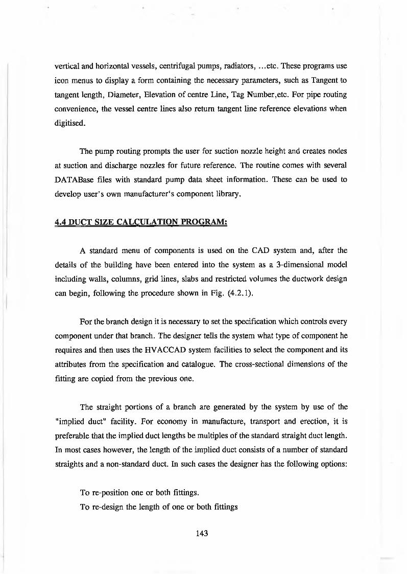
vertical and horizontal vessels, centrifugal pumps, radiators, ...etc. These programs use
icon menus to display a form containing the necessary parameters, such as Tangent to
tangent length, Diameter, Elevation of centre Line, Tag Number,etc. For pipe routing
convenience, the vessel centre lines also return tangent line reference elevations when
digitised.
The pump routing prompts the user for suction nozzle height and creates nodes
at suction and discharge nozzles for future reference. The routine comes with several
DATABase files with standard pump data sheet information. These can be used to
develop user’s own manufacturers component library.
4 . 4 D U C T S I Z E C A L C U L A T I O N P R O G R A M :
A standard menu of components is used on the CAD system and, after the
details of the building have been entered into the system as a 3-dimensional model
including walls, columns, grid lines, slabs and restricted volumes the ductwork design
can begin, following the procedure shown in Fig. (4.2.1).
For the branch design it is necessary to set the specification which controls every
component under that branch. The designer tells the system what type of component he
requires and then uses the HVACCAD system facilities to select the component and its
attributes from the specification and catalogue. The cross-sectional dimensions of the
fitting are copied from the previous one.
The straight portions of a branch are generated by the system by use of the
"implied duct" facility. For economy in manufacture, transport and erection, it is
preferable that the implied duct lengths be multiples of the standard straight duct length.
In most cases however, the length of the implied duct consists of a number of standard
straights and a non-standard duct. In such cases the designer has the following options:
To re-position one or both fittings.
To re-design the length of one or both fittings
143

To leave the end part as a non-standard straight.
To make a decision, the designer uses the AutoCAD facility which calculates the
number of standard straights and evaluates the remaining length. Once a branch has
been designed, the designer uses the grout facility to visually check whether the
components have been correctly positioned and whether they clash with any existing
branches or structure.
The final drawing has to be fully dimensioned and annotated before being sent
to the client for approval. The designer identifies the end points of a dimension and
then, automatically, the system draws a line with two end arrows and next to it, the
correct dimension. Most information is automatically drawn from the database but it is
also possible to input any other data, such as notes and reference drawing numbers.
At approval stage, the drawings are sent to the client for approval. The design,
although complete, contains no straight duct items as individual components but as
implied duct which is replaced by straights after approval.
Output for the factory includes a drawing, list of blank sizes required, costing,
production control data, and of course the individual information for each piece to be
cut. There is no optimisation program for nesting components in a sheet.
This program is also written in Autolisp language that is provided with the
AutoCAD Software. It is appropriately divided into the following sections:
• Interactively asking the user for the start and points of section of the duct
system layout.
• By using the Darcy-Weisbach and Colebrook equations and the ASCII file
from the load calculation, the duct work will be sized automatically.
• Friction loss in each section of the duct work will be stored in a data base for
the total system calculation later.
• Each section of ductwork will be checked against the user-inputted limiting
144
I

velocity and allowable ceiling clearance.
• Dimensions of each section of ductwork will be stored in the DATABase for
material take up purposes.
4.4.1 Duct sizing theoretical analysis:
The problem of sizing a duct reduces to the solution of a basic relationship
between v, the quantity of air flowing in m3/s, A, the cross-sectional area of the duct
in m2 and V, the mean velocity of airflow in m/s, given by the simple equation
Eq. (4.4.1) which is expressed as:
where:
A = Duct area, [m2].
V = Average velocity, [m/s].
The duct area may be calculated from:
Round duct:
v = A V (4.4.1)
a n D 2 A = ---- (4.4.2)4
where:
D = Duct diameter, [m].
Rectangular duct:
A = H W (4.4.3)
where:
H = Duct height, [m].
W = Duct width, [m].
Of the three variables in the equation, v is known from other considerations (
the required ventilation rate or the amount of air needed to offset a calculated sensible
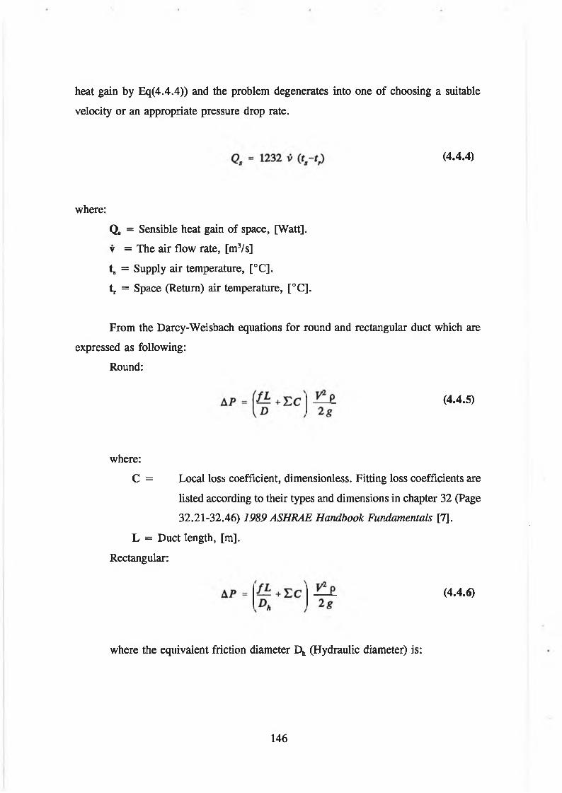
heat gain by Eq(4.4.4)) and the problem degenerates into one of choosing a suitable
velocity or an appropriate pressure drop rate.
(4.4.4)
where:
Q, = Sensible heat gain of space, [Watt],
v = The air flow rate, [m3/s]
t9 = Supply air temperature, [°C],
tr = Space (Return) air temperature, [°C].
From the Darcy-Weisbach equations for round and rectangular duct which are
expressed as following:
Round:
where:
C = Local loss coefficient, dimensionless. Fitting loss coefficients are
listed according to their types and dimensions in chapter 32 (Page
32.21-32.46) 1989 ASHRAE Handbook Fundamentals [7],
L = Duct length, [m].
Rectangular:
(4.4.5)
(4.4.6)
where the equivalent friction diameter I \ (Hydraulic diameter) is:
146

Di = 2 H W H + W
(4.4.7)
Substituting v/A into Darcy-Weisbach equations (Eq.(4.4.5), (4.4.6)) for the velocity
V to obtain the pressure drop of a single duct section in terms of diameter D and the
equivalent velocity diameter Dv for the round and rectangular ducts respectively, thus:
Round duct:
Rectangular duct:
A P = 0.881 H p v 2 ! ) 5
8(4.4.8)
A P = 0.881sP d :
g(4.4.9)
where (i is defined as:
Round Duct:
|x = f L + H C D (4.4.10)
Rectangular Duct:
D (4.4.11)
and the equivalent velocity diameter of a rectangular duct is calculated by Eq.(4.4.8)
as following;
Dy = N
4 H W (4.4.12)n
Since D and Dv are the same value for round and equivalent rectangular ducts,
147

flow can be defined in term of diameter and pressure loss by coefficient p. thus,
v = 1 . 1 1 0 7 U - f U p, 2)2.5 A F 0.5 ( 4 . 4 . 1 3 )
For calculation the friction factor/, the type of air flow in the duct must be
known which can be determined by Reynolds number which is calculated by:
ReD h V ( 4 . 4 . 1 4 )
where:
Dh = Hydraulic diameter, [m].
v = Kinematic viscosity (for the standard air v= ), [m2/s].
Within the region of laminar flow (Reynolds number less than 2000), the friction
factor is a function of Reynolds number only. For turbulent flow, the friction factor
depends on Reynolds number, duct surface roughness and internal hydraulic diameter.
The traditional Moody chart depicts the behaviour for round passages. For hydraulically
smooth ducts, the friction factor again depends only on Reynolds number, but the
dependence is markedly different from the laminar flow. In general, for non smooth
surfaces, the friction factor depends on roughness, Reynolds number and hydraulic
diameter. However, for a particular level of roughness beyond a sufficiently large
Reynolds number, the friction factor becomes independent of Reynolds number, and the
flow condition is considered as fully rough. Between the bounding limits of
hydraulically smooth behaviour and fully rough behaviour, is a transitional roughness
zone where the friction factor depends on both roughness and Reynolds number. In this
transitionally rough, turbulent zone, where most cases of air flow occur in air
conditioning applications, the friction fa c to r/is calculated By Colebrook’s equation.
Since this equation can not be solved explicitly for / , iterative techniques have to be
148

used:
— = - 2 logi f
2.513.7 A. R e if j
(4.4.11)
4.4.2 DUCTWORK p r o g r a m e x e c u t i o n s t e p s :
Here is how the program would work. The program would Initially load the
architectural plan on the PC Screen, by asking the user to enter the architect’s floor
plan file name, it would prompt the user to input the friction loss factor per 100 ft (30
m) of duct, the limiting velocity, the roughness of the sheet metal used, and the
allowable ceiling clearance dimension.
The program would then prompt the user for the start point of a duct system
layout as soon as this is entered the output file from the load calculation would be read,
and the overflow rate (v), would be used to calculate the duct size. It would prompt the
user to enter an end point to this section of the ductwork and duct work would be
drawn to the screen accordingly. Fittings such as elbows, transitions, dampers, and
turning vanes would be added automatically, based on selecting the type of fitting from
the duct fitting icon menu or dampers icon menu, the section would be added to them,
previous duct size, the directions of the next point as the next point, and the flow rate.
The initial inputs, such as the limiting velocity and ceiling clearance would act
as check figures to round off the duct size and to limit the duct height or diameter to
fit in the ceiling void. This interaction would be carried out until the user enters quit.
All the necessary data for friction loss calculation and material would be saved in a data
base while the quality interact was being carried out and the user can edit the output
using HVACSYS by calling it within HVACCAD interface by clicking the HVACSYS
command and then from this package can edit the results.
149
4.5 PSYCHROMETRIC CHART PROGRAM:
The theoretical analysis explained the work on psychrometric charts in the last
chapter in detail from defining a point to all air conditioning processes. The purpose
of designing this program is to make the work of the user easier to perform so that the
user can use special commands designed to cover all his work on a displayed
psychrometric chart which should be called as a DXF file. Considering the AutoCAD
coordinates X-Y and transfer them to psychrmetric chart coordinates where X axis
become as the dry bulb temperature t^ and Y axis as humidity ratio W axis, that have
been done by multiplying all temperature by 10 and all W values by 283.45.
4 . 5 . 1 PSYCHART PROGRAMME EXECUTION STEPS:
After the user selects the Psychart command from HVACCAD screen menu, or
by typing Psychart on the COMMAND: prompt, automatically the Psychart lisp
program will be loaded, and a prompt will ask the user the DXF file name which was
designed by HVACSYS Package. Then the user has to enter the DXF file name and
press Enter key. A full screen psychrometric chart will appear as shown in Fig.(4.10),
and also psychart screen menu will appear, then the user can work on the psychrometric
chart as he would work on the manual chart by selecting whatever he wants from three
commands P o i n t , P r o c e s s or W i n d o w . W i n d o w command is only for zooming with
defining a new board which has the values of parameters (t^, W).
If the user selects the P o i n t command, 13 commands (TDB&RH, TDB&TWB,
TDB&TDP, TDB&W, TDB&H, RH&TWB, RH&TDP, RH&W, RH&H, TWB&TDP,
TWB&W, TDP&H, W&H) will appear in the screen menu to define the state point.
The user has the mouse option to select the type of defining the state point. And, he has
also the COMMAND option to enter the two parameters to define the state point.
When the user selects P r o c e s s command (by clicking on the screen menu by the
mouse or typing it after COMMAND: prompt), a processes menu will appear on the
screen. The user has the option to select the type of process (General, Heating,
Cooling, Humidification, Zone, Mixing, and Collecting). Once the process is selected
, the prompt will ask the user to input the allowable combinations to define this process.
150

may be read directly into a components data record.
The HVACCAD program also offers in addition to graphics drawings, for the
complete system, a bill o f materials for each component with details and the whole
system costs are printed out.
152

CHAPTER FIVE
CASE STUDY AND VALIDATIONS
5.1 INTRODUCTION;
Although the calculation techniques of HVAC loads based on the physical laws
of energy and substance conservation is universally true, the computer codes derived
by applying this approach will not always be correct. In other words, certain differences
between the computed results and the reality can possibly exist. The reason for this is
that in every stage of calculations, it is impossible to define in detail and accurately
every energy and mass exchange, some less important facts are usually ignored and
assumptions are made in the design procedure. Therefore, validations of the packages
are important and necessary. From the validations, differences between the results of
the developed package and other commercial packages can be discovered and the
allowed difference caused by simplifications can then be confirmed.
Traditionally, the validation is proceeded by comparing the predictions from the
hand calculation method to the corresponding monitored results. Higher accuracy and
reliability can be expected from such validation provided. In this study, a comparison
between the developed package and other commercial package (Hevacomp) is presented.
The following sections will give the selective results from the developed package for
an building example previously designed by Seamus Homan Associates of Dublin.
5.2 CASE STUDY:
The example was an application of air conditioning system for a building built
153
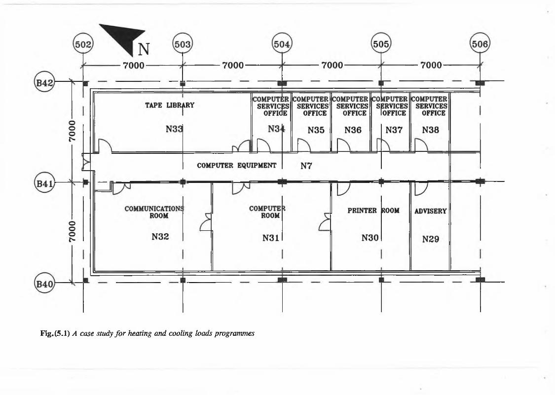
Fig.(5.1) A case study fo r heating and cooling loads programmes
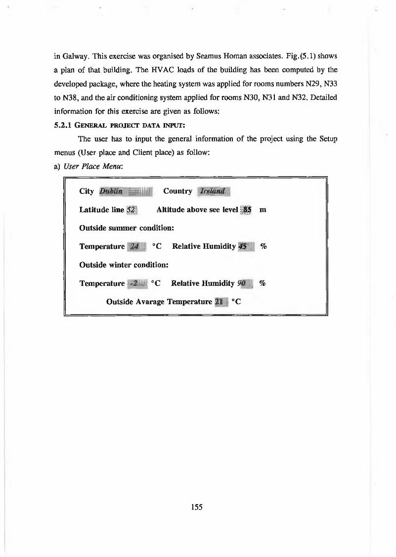
in Galway. This exercise was organised by Seamus Homan associates. Fig.(5.1) shows
a plan of that building. The HVAC loads of the building has been computed by the
developed package, where the heating system was applied for rooms numbers N29, N33
to N38, and the air conditioning system applied for rooms N30, N31 and N32. Detailed
information for this exercise are given as follows:
5.2.1 G eneral project data input:The user has to input the general information of the project using the Setup
menus (User place and Client place) as follow:
a) User Place M em :
C i t y Dublin H il l C o u n t r y W ^n d -.
L a t i t u d e l i n e § | § A l t i t u d e a b o v e s e e l e v e l ¡ ¡ ¡ § m
O u t s i d e s u m m e r c o n d i t i o n :
T e m p e r a t u r e 2 4 ° C R e l a t i v e H u m i d i t y 45' %
O u t s i d e w i n t e r c o n d i t i o n :
T e m p e r a t u r e 111111 ° C R e l a t i v e H u m i d i t y 90 ... %
O u t s i d e A v a r a g e T e m p e r a t u r e ¿ 1 | ° C
155

b) Client Place Menu:
D e s i g n e r K.A. Alwhban A d d r e s s School o f Mech. & Matm. Eng.
C i t y 9 C o u n t r y j j
C l i e n t M | | l A d d r e s s S I
C i t y GatM ? C o u n t r y Rep. o f IRELAND
P r o j e c t N a m e § | C ^ :;i. ¡ ¡ ¡ ¡ I | f ' T o t a l A r e a | | | § i | m 2
N u m b e r o f B u i l d i n g s | T H e a t i n g S a f e t y F a c t o r 10 %
B u i l d i n g O p e n i n g H o u r ¡ | j | S e n s i b l e S a f e t y F a c t o r 10 %
B u i l d i n g C l o s i n g H o u r | I | L a t e n t S a f e t y F a c t o r 10 %
The following table shows the room dimensions and its application( heating or
air-conditioning):
No. Description length[m]
Width[m]
Height[m]
System
N29 Advisory 2.8 6.3 2.7 Heating
N30 Printer room 5.6 6.3 2.7 Air Conditioning
N31 Computer room 8.4 6.3 2.7 Air Conditioning
N32 Communications room 8.4 6.3 2.7 Air Conditioning
N33 Tape library 11.2 4.2 2.7 Heating
N34-N38
Computer services offices
2.8 4.2 2.7 Heating
N7 Computer Equipment corridor
25.5 2 2.7 Heating
5.2.2 C a l c u l a t i o n o f U-V a l u e s :
156

Surface
To calculate the U-values for the building constructions, the user has to select
U-value command from the Program menu. In this case study there are six types of
surfaces listed as follows:
S u r f a c e 1 ( S I ) :
- layer of glass reinforced plastic
- 25 mm of insulation board - polysterene
S u r f a c e 2 ( S 2 ) :
- 100 mm brick outer leaf.
- 95 mm air cavity.
- 30 mm insulation board-polystyrene
- 100 mm concrete block
- 1 3 mm plaster - 20AT
S u r f a c e 3 ( S 3 ) :
- 2 mm steel panel
- 25 mm polystyrene insulation board
- 2 mm steel panel
S u r f a c e 4 ( S 4 ) :
- 100 mm block internal partition
S u r f a c e 5 ( S 5 ) :
- 10 mm steel
- 25 mm spray on insulation thick
S u r f a c e 6 ( S 6 ) :
- double glazing in steel frame type unknown.
S u r f a c e 7 ( S 7 ) :
- Solid ground floors for each room.
The results obtained from the developed package are listed as follows:
1 (SI):
External Wall Outside Thermal Resistance .05 [m2°C/W]Inside Thermal Resistance .123 [m2°C/W]
157
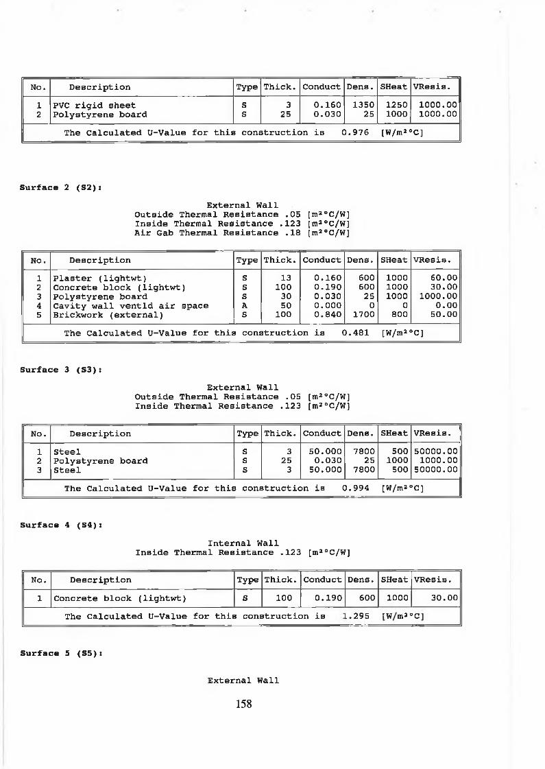
No. Description Type Thick. Conduct Dens. SHeat VResis.1 PVC rigid sheet S 3 0.160 1350 1250 1000.002 Polystyrene board S 25 0.030 25 1000 1000.00
The Calculated U-Value for this construction is C). 976 [W/m2 °C]
Surface 2 (S2):External Wall
Outside Thermal Resistance .05 [m2°C/W] Inside Thermal Resistance .123 [m2°C/W] Air Gab Thermal Resistance .18 (m2°C/W)
No. Description Type Thick. Conduct Dens. SHeat VResis.1 Plaster (lightwt) S 13 0.160 600 1000 60.002 Concrete block (lightwt) S 100 0.190 600 1000 30.003 Polystyrene board S 30 0.030 25 1000 1000.004 Cavity wall ventld air space A 50 0.000 0 0 0.005 Brickwork (external) S 100 0.840 1700 800 50.00
The Calculated U-Value for this construction is (). 481 [W/m2 °C]
Surface 3 (S3):External Wall
Outside Thermal Resistance .05 [m2°C/W] Inside Thermal Resistance .123 [m2°C/W]
No. Description Type Thick. Conduct Dens. SHeat VResis.1 Steel S 3 50.000 7800 500 50000.002 Polystyrene board S 25 0.030 25 1000 1000.003 Steel S 3 50.000 7800 500 50000.00
The Calculated U-Value for this construction is (). 994 [W/m2 °C]
Surface 4 (S4):Internal Wall
Inside Thermal Resistance .123 [m2°C/W]
No. Description Type Thick. Conduct Dens. SHeat VResis.1 Concrete block (lightwt) S 100 0.190 600 1000 30.00
The Calculated U-Value for this construction is L.295 si 3 M O O
External Wall
Surface 5 (S5):
158

Outside Thermal Resistance .05 (m2°C/W] Inside Thermal Resistance .123 [m20C/W]
No. Description Type Thick. Conduct Dens. SHeat VResis.1 Polyurethane foam S 25 0.026 30 1000 60.002 Steel S 10 50.000 7800 500 50000.00
The Calculated U-Value for this construction is (). 882 [W/m2 °C]
In the package used by Homan Associates the U-value of the floor is considered
to be valid for the whole building (they treat the whole building as one room), and they
take this value as an average value for all rooms. Their results are as follows;
a. Solid ground floor (four exposed edges):
Solid Ground Floor Four Exposed Edges
The Calculated U-Value for this construction is 0.487 [W/m2°C]
b. Solid ground floor (Two Perpendicular exposed edges):
Solid Ground Floor Two Perpendicular Exposed Edges
The Calculated U-Value for this construction is 0.276 [W/m2°C]
Then they calculated the average value of the two components as:
U = °-4- 7 - 0 276 = 0.3822
In fact the U-value of each room differs from this average value, and this will
not give a correct load for the floor. The U-value must be calculated for the floor of
each room separately. The following results show the U-value of the floor of each
room:
159
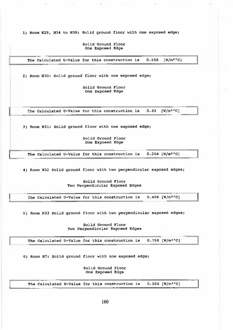
1) Room N29, N34 to N38: Solid ground floor with one exposed edge;
Solid Ground Floor One Exposed Edge
The Calculated U-Value for this construction is 0.558 [W/m2 °C]
2) Room N30: Solid ground floor with one exposed edge;
Solid Ground Floor One Exposed Edge
The Calculated U-Value for this construction is 0.33 [W/m2 °C]
3) Room N31: Solid ground floor with one exposed edge;
Solid Ground Floor One Exposed Edge
The Calculated U-Value for this construction is 0.264 [W/m2 °C]
4) Room N32 Solid ground floor with two perpendicular exposed edges;
Solid Ground Floor Two Perpendicular Exposed Edges
The Calculated U-Value for this construction is 0.498 [W/m2 °C]
5) Room N33 Solid ground floor with two perpendicular exposed edges;
Solid Ground Floor Two Perpendicular Exposed Edges
The Calculated U-Value for this construction is 0.758 [W/m2 °C]
6) Room N7: Solid ground floor with one exposed edge;
Solid Ground Floor One Exposed Edge
The Calculated U-Value for this construction is 0.264 3 w o O
160
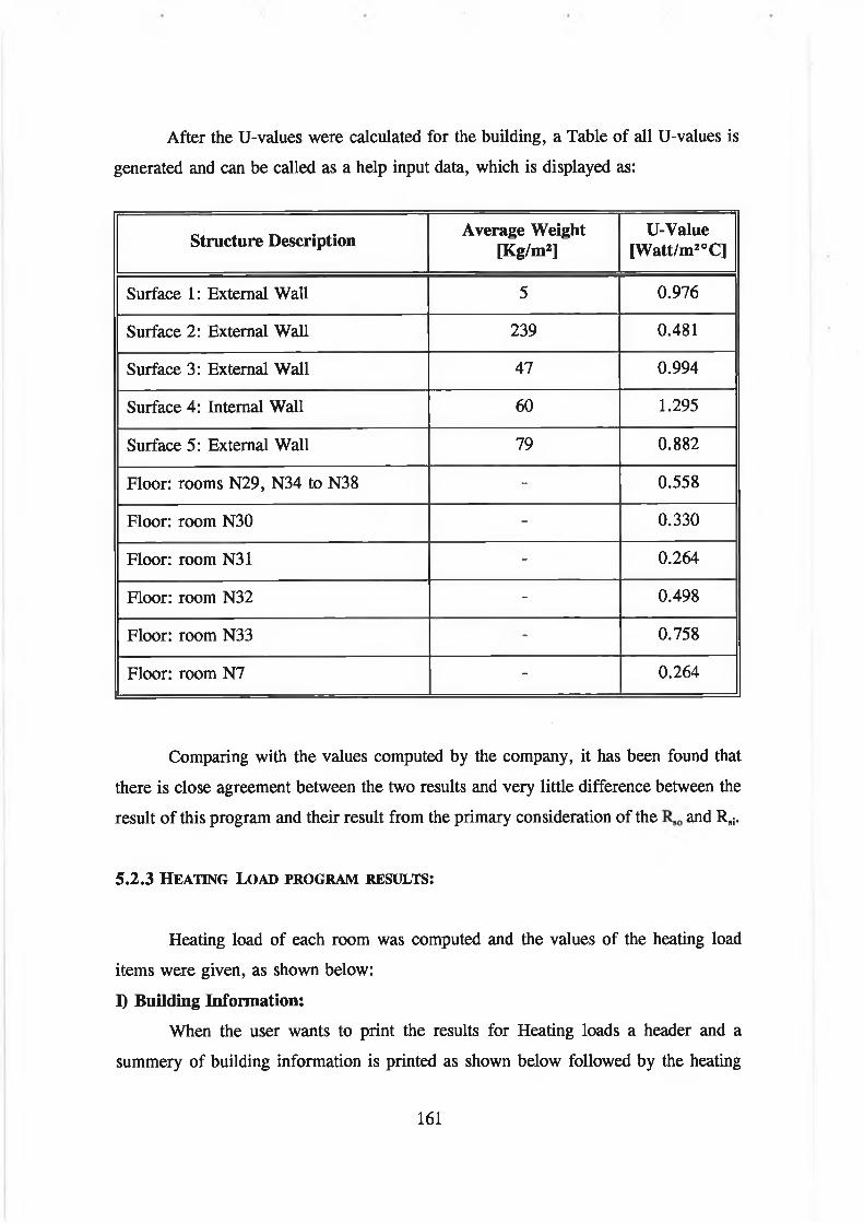
After the U-values were calculated for the building, a Table of all U-values is
generated and can be called as a help input data, which is displayed as:
S t r u c t u r e D e s c r i p t i o nA v e r a g e W e i g h t
[ K g / m 2]U - V a l u e
[ W a t t / m 2 °C]
Surface 1: External Wall 5 0.976
Surface 2: External Wall 239 0.481
Surface 3: External Wall 47 0.994
Surface 4: Internal Wall 60 1.295
Surface 5: External Wall 79 0.882
Floor: rooms N29, N34 to N38 - 0.558
Floor: room N30 - 0.330
Floor: room N31 - 0.264
Floor: room N32 - 0.498
Floor: room N33 - 0.758
Floor: room N7 - 0.264
Comparing with the values computed by the company, it has been found that
there is close agreement between the two results and very little difference between the
result of this program and their result from the primary consideration of the and Rsi.
5.2.3 H e a t i n g L o a d p r o g r a m r e s u l t s :
Heating load of each room was computed and the values of the heating load
items were given, as shown below:
I ) B u i l d i n g I n f o r m a t i o n :
When the user wants to print the results for Heating loads a header and a
summery of building information is printed as shown below followed by the heating
161

load output for each room:
H V A C S Y S Designer School of Mechanical and Manufacturing Engineering, Dublin City University
Developed by KASSEM ALWAHBAN, SSRC, P.O.BOX 4470, Damascus, Syria Project: UCG Design: K. ALWAHBAN Dates 12-21-1992
North Latitude L - 52 °Altitude above sea level h = 85 m
Outside Dry-Bulb Temperature Tdo = -2 °C Outside air humidity ratio RHo = 9 0 %
162

H) Room N29:
The input:
Building No. 1 Storey No. 1 Space No. 1Dimension LxWxH 2.8x63x2.7 Description ¡¡¡¡¡|Dry Bulb Temperature tdb 21.0 °C Relative Humidity |
Roof Information U-Value (W/m2oC) | |
SkyLight U-Value 0,000 Walls Information
Roof Area (m2) SkyLight Area
%
Suspended (Y/N) | | Temp. Diff |¡§ ¡
Wall No. 1 2 3 4 5 6 7 8W1 Orientations SW p i p ¡ I nW1 Area (m2) ( ¡ 1 1.74 7.56 0.00 0.00 r i i 0.00 n i lW1 U-Value S Ü 0.973 L295 0.0 | 0.0 i t o 0.000 0.000W1 (1-Ex, 2-In, 3-Bs) J Jg j “J I i 0Gl Area 3.47 o.oo o.oo o;oo o.oo 0.00 0.Û0 10.00Gl U-Value I I ® 0.000 0.000 0:000 0.000 0.000 0.000 0,.qopWind & Orien. Factor IQ m ■ T | ■ 0 0 0Partition Temp. Diff $.0 .0.0 i t0 0,0 0.0
Floor Information0.0 0,0 "
Area (m2) 17.64 U-Value(W/m2oC) 0.558 Temp. Diff 1Type (l-Inter,2-Solid Grnd.,3-Bs) f
Infiltration (1-Air Changes,2-Crack) | Air Changes No. î .5 Crack Lneth M B Ventilation (1-Air Chngs,2-CFM/Person) 0 Air Chngs No 0.Ö CFM/Person 0.0
The result:
Room N29 : Advisory Inside Dry-Bulb Temperature Tdi = 21 °CInside air humidity ratio RHi = 50 %
Construction Type Area U-Value 6t q Wind Factor QWall No. 1 , SW Glass No. 1 , SW Wall No. 2 , SW Wall No. 3 , NE Ground Floor
ExternalExternalExternalInternalSolid
4.13.5 1.77.6
17.6
0.48103.20000.97301.29500.5580
23.023.023.0 3.0
23.0
45.4255.4 38.929.4
226.4
10101000
49.89280.9342.8329.37
226.39Sensible heat loss through infiltration . Latent heat loss throuah infiltration ...
QSInfil = OSInfil =
565.80295.02
Sum of heat losses from the room QTotal = 1490.24-Total sensible heat loss for the room is ... -Total latent heat Loss for the room is ....
... QStotal = 1195 WattWatt
-Total heat loss for the room is ..... Watt
163

Ill) Room N30:
The input:
Building No. 1 Storey No. 1 Space No. 2Dimension LxWxH 5ÜSx6.3x2.7 Description N30 : Printer Room Dry Bulb Temperature tdb SÜ.0 °C Relative Humidity 50 %
Roof InformationRoof Area (m2) 0.00 U-Value (W/m2oC) 0.000 Suspended (Y/N) ff SkyLight Area 0.00 SkyLight U-Value 0,000 Temp. P iff IM
Walls InformationWall No. 1 2 3 4 5 6 7 8W1 Orientations i n Pi HP Ü &ÉÉÉ II 111!W1 Area (m2) 8.18 3.47 15.12 0.00 111 ili till wmW1 U-Value £481 0.973 L295 0.0 0.0 0.0 0.000 0.000W1 (1-Ex,2-In,3-Bs) 1 1 III J 8 i .1 0Gl Area 6.94 0.00 0.00 0.00 0.00 Ill 0.00 niGl U-Value 3,200 0.000 0,000 0.000 0.000 0.000 0.000 0.000Wind & Orien. Factor 10 1° o jl ■ ■ m 0Partition Temp. Diff B l 0 .0 13 .0 0,0
Floor informationill 0.0 1É1 0.0
Area (m2) 1ÜI18 U-Value(W/m2oC) 0.330 Temp. Diff mType (1-Inter,2-Solid Grnd.,3-Bs) f
Infiltration (1-Air Changes,2-Crack) | Air Changes No. 1.5 Crack Lngth 0.0 Ventilation (1-Air Chngs,2-CFM/Person) p Air Chngs No.0,0 CFM/Person 0,0
The result:
Room N30 : Printer Room Inside Dry-Bulb Temperature Tdi = 21 °CInside air humidity ratio RHi = 50 %
Construction Type Area U-Value 6t q Wind Factor QWall No. 1 , SW Glass No. 1 , SW Wall No. 2 , SW Wall No. 3 , NE Ground Floor
ExternalExternalExternalInternalSolid
8.26.93.515.135.3
0.48103.20000.97301.29500.3300
23.023.023.0 3.0
23.0
90.5510.877.758.7
267.8
10101000
99.54561.8685.4258.74
267.78Sensible heat loss through infiltration . Latent heat loss through infiltration ...
QSInfil - OSInfil -
1119.81583.90
Sum of heat losses from the room QTotal - 2777.05-Total sensible heat loss for the room is ... -Total latent heat Loss for the room is ....
WattWatt
-Total heat loss for the room is ..... Watt
164
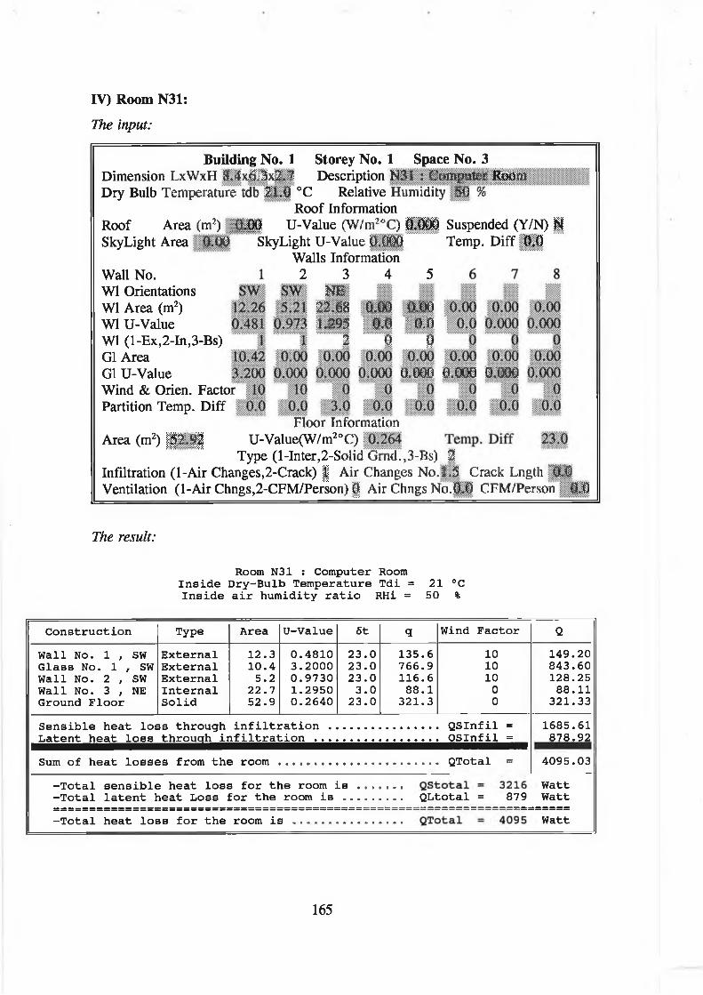
The input:
IV) Room N31:
Building No. 1 Storey No. 1 Space No. 3Dimension LxWxH 8.4x&3x2.7 Description N31 : Computer Room Dry Bulb Temperature tdb 21.0 °C Relative Humidity 50 %
Roof Information M U U-Value (W/m2oC) 0.000 Suspended (Y/N) 1
SkyLight U-Value 0,000 Walls Information
2
Temp. Diff 0,0
3 4 5NE
22.68 0.00 0.001.295 0.0 * 0,0
2 i 1
Roof Area (m2)SkyLight Area 0.00
Wall No.W1 Orientations W1 Area (m2)W1 U-Value W1 (1-Ex,2-In,3-Bs)G1 Area Gl U-Value Wind & Orien. Factor Partition Temp. Diff
Area (m2) | | 2 . | | U-Value(W/m2°C)Type (1-Inter,2-Solid Gmd.,3-Bs) 2
Infiltration (1-Air Changes,2-Crack) j Air Changes No.1.5 Crack Lngth Ö.Ö Ventilation (1-Air Chngs,2-CFM/Person) | Air Chngs No.0.0 CFM/Person 0.0
Floor Information2o/
0 . 0 0 0 0.000 0.000
The result:
Room N31 : Computer Room Inside Dry-Bulb Temperature Tdi = 21 °CInside air humidity ratio RHi = 50 %
Construction Type Area U-Value 5t q Wind Factor QWall No. 1 , SW Glass No. 1 , SW Wall No. 2 , SW Wall No. 3 , NE Ground Floor
ExternalExternalExternalInternalSolid
12.310.4 5.2
22.752.9
0.48103.20000.97301.29500.2640
23.023.023.0 3.0
23.0
135.6 766.9116.6 88.1
321.3
10101000
149.20843.60128.2588.11
321.33Sensible heat loss through infiltration . Latent heat loss throuah infiltration ...
QSInfil = OSInfil =
1685.61878.92
Sum of heat losses from the room QTotal = 4095.03-Total sensible heat loss for the room is ... -Total latent heat Loss for the room is .... . .. QLtotal = 879
WattWatt
-Total heat loss for the room is ..... Watt
165
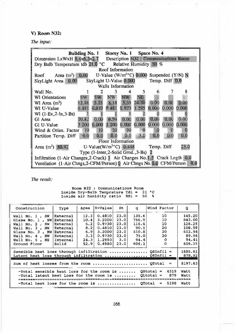
The input:
V) Room N32:
Building No. 1 Storey No. 1 Space No. 4Dimension LxWxH 8.4x6 J x & l Description M32 j Communications RooiiJ Dry Bulb Temperature tdb 21.0 °C Relative Humidity 50 %
Roof InformationRoof Area (m2) 0.00 U-Value (W/m2oC) l i H i Suspended (Y/N) | SkyLight Area 0.00 SkyLight U-Value 0.000 Temp. Diff 0.0
Walls InformationWall No. 1 2 3 4 5 6 7 8W1 Orientations SW 1 1 1 NW NE MW1 Area (m2) 12,26 5.2? S B p i 2 4 M P i i o.oc 100W1 U-Value 0,48 i 0.973 0,481 0,973 1.295 0.000 O.OQOj
W1 (1-Ex,2-In,3-Bs) j | " i 1 J 1 eGl Area 10.42 I Ü § 6.94 0,00 0.00 0.0Ò o.oc I 1 Ì É
Gl U-Value 3.20Ö 0.000 3.200 0.000 0.000 n -■ X
;
0.0ÜWind & Orien. Factor ¡| | 10 " m M m 1 1 Ü 0Partition Temp. Diff l l p i 0.0 Ö.0 ¡ 1 1 1 1 1 1 0.0 m m o ,o
Floor InformationArea (m2) 52.92 U-Value(W/m2oC) &498 Temp. Diff m m
Type (1-Inter,2-Solid Gmd.,3-Bs) i Infiltration (1-Air Changes,2-Crack) | Air Changes No. 1.5 Crack Lngth 0.0 Ventilation (1-Air Chngs,2-CFM/Person) | Air Chngs No.0.0 CFM/Person 0.0
The result:
Room N32 : Communications Room Inside Dry-Bulb Temprature Tdi = 21 °C Inside air humidity ratio RHi = 50 %
Construction Type Area U-Value 5t q Wind Factor QWall No. 1 , SW External 12.3 0.4810 23.0 135.6 10 149.20Glass No. 1 , SW External 10.4 3.2000 23.0 766.9 10 843.60Wall No. 2 , SW External 5.2 0.9730 23.0 116.6 10 128.25Wall No. 3 , NW External 8.2 0.4810 23.0 90.5 20 108.59Glass No. 3 , NW External 6.9 3.2000 23.0 510.8 20 612.94Wall No. 4 , NW External 3.3 0.9730 23.0 75.0 20 89.96Wall No. 5 , NE Internal 24.3 1.2950 3.0 94.4 0 94.41Ground Floor Solid 52.9 0.4980 23.0 606.1 0 606.15Sensible heat loss through infiltration . QSInfil = 1685.61Latent heat loss through infiltration ... OSInfil = 878.92Sum of heat losses from the room QTotal = 5197.63
-Total sensible heat loss for the room is ... Watt-Total latent heat Loss for the room is Watt-Total heat loss for the room is ...... Watt
166

VD Room N33:
The input:
Building No. 1Dimension LxWxH W [
O g
Space No. 5Storey No. 1Description |
Dry Bulb Temperature tdb ÎU.0 °C Relative HumidityRoof Information
U-Value (W/m20C) 0.000 Suspended (Y/N) fgRoof Area (m2) SkyLight Area 0 .0 SkyLight U-Value 0.000
Walls InformationWall No.W1 Orientations W1 Area (m2)W1 U-Value W1 (1-Ex,2-In,3-Bs)G1 Area Gl U-Value Wind & Orien. Factor
...ggssa
Partition Temp. Diff |Floor Information
Area (m2) 4%04 U-Value(W/m2oC) 0.75$Type (1-Inter,2-Solid Grnd.,3-Bs) 2
Infiltration (1-Air Changes,2-Crack) | Air Changes No. 1.5 Crack Lngth 0.0 Ventilation (1-Air Chngs,2-CFM/Person) | Air Chngs No.0.0 CFM/Person 0.0
The result:
Room N33 : Tapes Library Inside Dry-Bulb Temperature Tdi = 21 °CInside air humidity ratio RHi = 50 %
Construction Type Area U-Value 6t q Wind Factor Q
Wall No. 1 , NW External 6 . 1 0 . 4 8 1 0 2 3 . 0 6 7 . 8 20 8 1 . 3 8Glass No. 1 , NW External 5 . 2 3 . 2 0 0 0 2 3 . 0 3 8 3 . 5 20 4 6 0 . 1 5Wall No. 2 , NW External 2 . 6 0 . 9 7 3 0 23.0 58.2 20 69.82Wall No. 3 , NE External 16.4 0.4810 23.0 180.9 20 217.06Glass No. 3 , NE External 13.9 3.2000 23.0 1022.3 20 1226.76Wall No. 4 , NE External 6.9 0.9730 23.0 155.3 20 186.37Wall No. 5 , SW Internal 30.2 1.2950 3.0 117.5 0 117.48Ground Floor Solid 47.0 0.7580 2 3 . 0 820.1 0 820.10Sensible heat loss through infiltration . QSInfil = 1497.01Latent heat loss throuoh infiltration ... OSInfil = 780.58Sum of heat losses from the room QTotal = 5456.71
-Total sensible heat loss for the room is ... Watt-Total latent heat Loss for the room is Watt-Total heat loss for the room is ..... Watt
167
!

The input:
VH) Room N34-N38:
Building No. 1 Storey No. 1 Space No. 6Description N34-N38 : S e r v tû f f iü l^ y S
Dry Bulb Temperature tdb 21.0 °C Relative Humidity 50 %Roof Information
| U-Value (W/m2oC) 0.000 Suspended (Y/N) | SkyLight U-Value 0,000 Temp. Diff 0 ,0
Walls Information
Dimension LxWxH
Roof Area (m2) SkyLight Area
m t c
0 ,(
Wall No.W1 Orientations W1 Area (m2)W1 U-Value W1 (1-Ex,2-In,3-Bs) Gl Area Gl U-Value Wind & Orien. Factor Partition Temp. Diff
Area (m2) ¡§¡¡p$
8
I0.00 0.00
0 .0 0 0 0 ,0 0 0
20 0mm |f§ |
Floor Information U-Value(W/m2oC) 0.558
Type (1-Inter,2-Solid Grnd.,3-Bs)
I0 .0 0
0,000'ìli
i l l
10.00 I p 0 .0 0 0 0 .0 0 0
0 > 0 0
0 .0 0 0
¡ I 0 0
"0 ,0 0
0 .0 0 0
■m m
0 .0 0
pffiiI¡Ili
olii0
0.0
Temp. Diff1
I0 * 0 0
o S Ü0
l i l i
H l
Infiltration (1-Air Changes,2-Crack) | Air Changes No. 1.5 Crack Lngth 0.0 Ventilation (1-Air Chngs,2-CFM/Person) 0 Air Chngs No.0,0 CFM/Person 0.0
The result:
Room N34-N38 : Services Offices Inside Dry-Bulb Temperature Tdi = 21 °CInside air humidity ratio RHi = 50 %
Construction Type Area U-Value 6t q Wind Factor Q
’'
(Jail No. 1 , NE »lass No. 1 , NE rfall No. 2 , NE (fall No. 3 , SW »round Floor
ExternalExternalExternalInternalSolid
5 . 21 . 70 . 67 . 6
1 1 . 8
0 . 4 8 1 03 . 2 0 0 00 . 9 7 3 01 . 2 9 5 00 . 5 8 8 0
2 3 . 02 3 . 02 3 . 0
3 . 02 3 . 0
5 7 . 51 2 8 . 1
1 4 . 32 9 . 4
1 5 9 . 0
202020
00
6 9 . 0 31 5 3 . 6 8
1 7 . 1 92 9 . 3 7
1 5 9 . 0 4
Sensible heat loss through infiltration . Latent heat loss throuah infiltration ...
QSInfil = OSInfil =
3 7 7 . 2 01 9 6 . 6 8
Sum of heat losses from the room QTotal = 1 0 0 2 . 1 9
-Total sensible heat loss for the room is ... -Total latent heat Loss for the room is ....
WattWatt
-Total heat loss for the room is ..... Watt
168

The input:
VIII) Room N7:
Building No. 1 Storey No. 1 Space No. 7Dimension LxWxH 25.5x2*0x2*7 Description N7 : Computer Equipment
Dry Bulb Temperature tdb 21.0 °C Relative Humidity ¡¡jH %Roof Information
Roof Area (m2) 0,00 U-Value (W/m2oC) 0*000 Suspended (Y/N) |f SkyLight Area 0.00 SkyLight U-Value 0.000 Temp. Diff 0.0
1
Walls Information 2 3 4
1 °’9?i a°°o °,0°c °'00 °’~ a0° °'00IWÊ 0.00 0,00 0.00 0.00 0.00 0.00 0.00 — o .o o o 6 *0 0 0 p m 0 .0 0 0 0 .0 0 0 0 .0 0 0 o . o r
Wall No.W1 Orientations W1 Area (m2)W1 U-Value W1 (1-Ex,2-In,3-Bs)G1 Area G1 U-ValueWind & Orien. Factor ÄPartition Temp. Diff f|0*0 0,0 0*0 ö*ö 4*0 f 0*0 "MM 11111
Floor Information Area (m2) H i U-Value(W/m2oC) 0,264
Type (1-Inter,2-Solid Gmd. ,3-Bs) §Infiltration (1-Air Changes,2-Crack) | Air Changes No. 1,5 Crack Lngth 0.0
The result:
Room N7 s Computer Equipment Inside Dry-Bulb Temperature Tdi = 18 °CInside air humidity ratio RHi = 50 %
Construct ion Type Area U-Value 5t q Wind Factor Q
Wall No. 1 , NW Glass No. 1 , NW Wall No. 2 , NW Ground Floor
ExternalExternalExternalSolid
1.95.71.7
51.0
0.48103.20000.97300.2640
20.020.020.023.0
18.2362.933.9
309.7
2020200
21.82435.4640.63
309.67Sensible heat loss through infiltration . Latent heat loss through infiltration ...
QSInfil = OSInfil =
1414.50616.04
Sum of heat losses from the room QTotal = 2838.12-Total sensible heat loss for the room is ... -Total latent heat Loss for the room is ....
QStotal = 2222 WattWatt
-Total heat loss for the room is ..... Watt
169
,

5.2.4 C o o l i n g l o a d p r o g r a m r e s u l t s :
The cooling load for rooms N30, N31 and N32 was computed according to
ASHRAE method (CLTD/CLF method). The information for each room is entered via
the Entry-input-data-menu. The results automatically appears on the screen and the user
has a choice to save the result and/or to print them. The input data and the results for
each room were printed as follows:
I ) B u i l d i n g I n f o r m a t i o n :
H V A C S Y S Designer School of Mechanical and Manufacturing Engineering, Dublin City University
Developed by KASSEM ALWAHBAN, SSRC, P.O.Box 4470, Damascus, Syria Project: UCG Design: K. ALWAHBAN Date: 12-21-1992
North Latitude L = 52 °Altitude above sea level h = 85 m
Outside Dry-Bulb Temperature Tdo = 2 4 °C Outside air humidity ratio RHo = 4 5 %
170
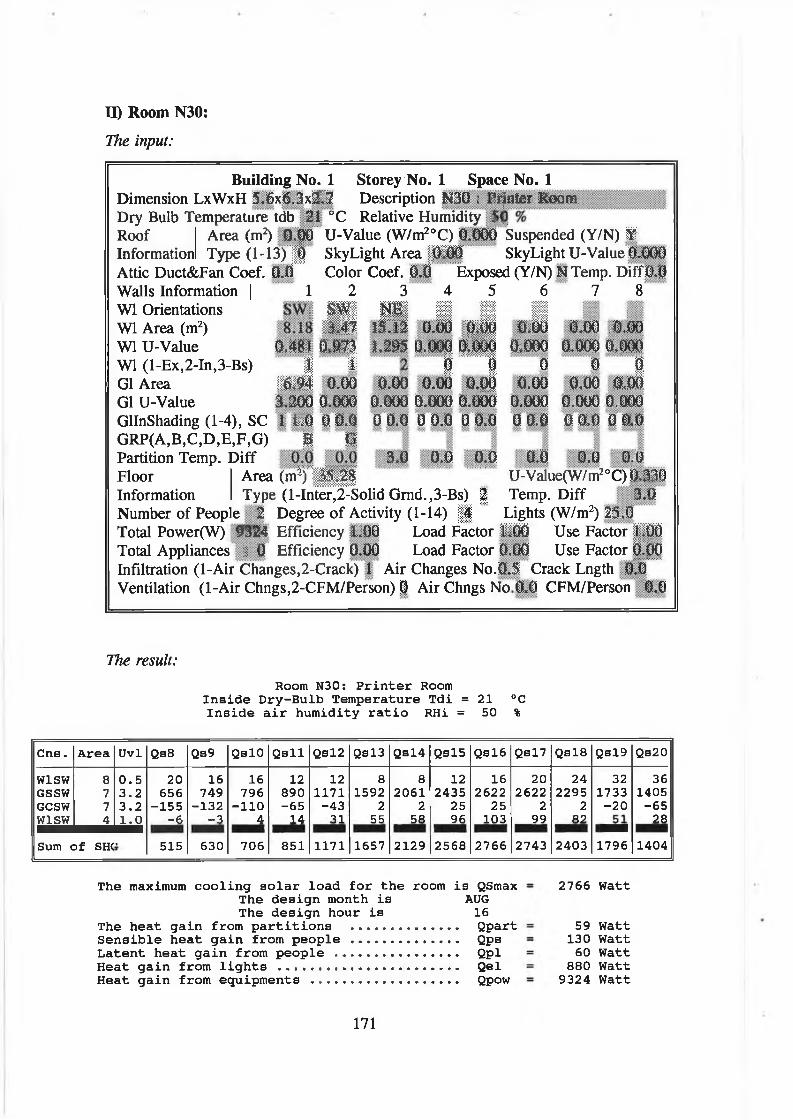
II) Room N30:
The input:
B u i l d i n g N o . 1 S t o r e y N o . 1 S p a c e N o . 1Dimension LxWxH 5.6x6.3x2.7 Description N30 : Printer RoomDry Bulb Temperature tdb 21 °C Relative Humidity tRoofInformation Attic Duct&Fan Coef. Walls Information | W1 Orientations W1 Area (m2)W1 U-Value W1 (1-Ex,2-In,3-Bs)G1 Area G1 U-Value GllnShading (1-4), SC GRP(A,B,C,D,E,F,G) Partition Temp. Diff FloorInformation
Area (m2) 0.00 U-Value (W/m2oC) 0,000 Suspended (Y/N) Y Type (1-13)J§! SkyLight A re a J M I SkyLight U-Value 0-000
0.0 Color Coef. 0.0 Exposed (Y/N) N Temp. Diff0,01 2■
i l l iù , m o , m
I I I I P 0 .0 0
3.200 0.000 1 LO 0 0.0
■ m
3 4 5 6
■ ■ ■ ■ 15.12 0.00 I I I 0;001 . 2 9 5 o .o o o o *d o d 0 ,0 0 0
I — I 0
0.00 0.00 0 .0 0.00 0.000 0.000 0.000 0.000 0 0.0 0 0.0 0 0.0 0 0.0
3.0 0.0 0.0 0.0
7 8
0 .0 0 .0 .0 0
0 .0 0 0 0 ,0 0 0 0 ' I 0,00 0,00
0 .0 0 0 0 .0 0 0
0 0 ,0 0 0 .0
0.0 0,0Area ( m T i l l l f ..........U-Value(W/m?0C) 0.330Type (1-Inter,2-Solid Gmd.,3-Bs) § Temp. Diff 3.0
Number of People 2 Degree of Activity (1-14) |§ Lights (W/m2) 25;0 Total Power(W) 9324 Efficiency LOO Load Factor MO Use FactorJ HTotal Appliances f 0 Efficiency 0.00 Load Factor 0,00 Use Factor 0.00Infiltration (1-Air Changes,2-Crack) 1 Air Changes No.0.5 Crack Lngth 0,0 Ventilation (1-Air Chngs,2-CFM/Person) 0 Air Chngs No 0.0 CFM/Person 0.0
The result:Room N30: Printer Room
Inside Dry-Bulb Temperature Tdi = 21 °C Inside air humidity ratio RHi = 50 %
Cns. Area Uvl Qs8 Qs9 QslO Qsll Qsl2 Qsl3 Qsl4 Qsl5 Qsl6 Qsl7 Qsl8 Qsl9 Qs20W1SW 8 0.5 20 16 16 12 12 8 8 12 16 20 24 32 36GSSW 7 3.2 656 749 796 890 1171 1592 2061 2435 2622 2622 2295 1733 1405GCSW 7 3.2 -155 -132 -110 -65 -43 2 2 25 25 2 2 -20 -65W1SW 4 1.0 -6 -3 4 14 31 55 58 96 103 99 82 MB 28Sum c3f SHCi 515 630 706 851 1171 1657 2129 2568 2766 2743 2403 1796 1404
The maximum cooling solar load for the room is QSmax The design month is AUGThe design hour is 16
The heat gain from partitions .............. QpartSensible heat gain from people .............. QpsLatent heat gain from people ................ QplHeat gain from lights ....................... QelHeat gain from equipments ................... Qpow
2766 Watt
59 Watt 130 Watt60 Watt
880 Watt9324 Watt
171

Sensiple heat gain from infiltration ....... QSinf = 146 WattLatent heat gain from infiltration...... QLinf = 75 Watt
-Total-Total
sensible heat gain for the room is latent heat gain for the room is .....
13305135
WattWatt
-Total heat gain for the room is ............. 13440 Watt
III) Room N31:
The input:
Building No. 1 Storey No. 1 Space No. 2Dimension LxWxH &4x6,3x2*7 Description N31 : Computer RoomDry Bulb Temperature tdb 21 °C Relative Humidity 50 %Roof I Area (m2) 0,00 U-Value (W/m2oC) 0.000 Suspended (Y/N) Y Information! Type (1-13) 0 Skylight Area 0.00 SkyLight U-Value i | | Attic Duct&Fan Coef. 0,0 Color Coef. | | l f Exposed (Y/N) NTemp. D if f ll lWalls Information | 1 2W1 Orientations g MW1 Area (m2) 12.26 5.21W1 U-Value 0.481 0.973W1 (1-Ex, 2-In, 3-Bs) 1 1G1 Area 10.42 0.00G1 U-Value 3.2«) 0.000GllnShading (1-4), SC | | |GRP(A,B,C,D,E,F,G)Partition Temp. Diff ;
2
3 4 5 6 7 8N i l
22M ¡ p ! p o o 0.00 0.00 :o 8
1.295 0.000 0.000 0.000 0.000 0.000i 0 0 0 0 0
P i i 0.00 0.00 $<00 0.00 0.00Ö.000 0.000 0.000 0.000 0.000 0.0000 0.0 0 0.0 1 0.0 I I I 0 0.0 o o .o ;
3.0 1 1 1 : 0 * 0 0,0 o : o i j
Ü-Value(W/m7< C) 0..lid Gmd.,3-Bs) | Temp. Diff 3.
Floor Area (nr)Information Type (l-IiNumber of People 3 Degree of Activity (1-14) | | Lights (W/m2) 25.0 Total Power(W) 36684 Efficiency 1,00 Load Factor 1.00 Use Factor LOGTotal Appliances 0 Efficiency 1111 Load Factor 0,00 Use Factor 0,00Infiltration (1-Air Changes, 2 -C rack )| Air Changes No.Q.5 Crack Lngth I IS F " Ventilation (1-Air Chngs,2-CFM/Person) | Air Chngs No.0.0 CFM/Person 0.0
The result:Room N31 : Computer Room
Inside Dry-Bulb Temprature Tdi = 21 °C Inside air humidity ratio RHi = 50 %
Cns. Area Uvl Qs8 Qs9 QslO Qsll Qsl2 Qsl3 Qsl4 Qsl5 Qsl6 Qsl7 Qsl8 Qsl9 Qs20W1SWGSSWGCSWW1SW
1210105
0.53.23.21.0
30974
-230-10
241113-196
-5
241183-163
6
181322-9721
181739-6346
122366
381
123061
387
183618
37142
243896
37152
303896
3H I
363409
3122
482574-3076
542087-9741
Sum cjf SHC( 764 936 1050 1264 1740 2462 3163 3815 4109 4076 3570 2668 2085
172

The maximum cooling solar load for the room is QSmax The design month is AUGThe design hour is 16
The heat gain from partitions ..... QpartSensible heat gain from people .............. QpsLatent heat gain from people ................ QplHeat gain from lights ....................... QelHeat gain from equipments ................... QpowSensible heat gain from infiltration ....... QSinfLatent heat gain from infiltration.......... QLinf
4109 Watt
88 Watt 195 Watt 90 Watt
1323 Watt 36684 Watt
73 Watt 38 Watt
-Total-Total
sensible heat gain for the room is latent heat gain for the room is .....
WattWatt
-Total heat gain for the room is ............. Watt
IV) Room N32:
The input:
Building No. 1 Storey No. 1 Space No. 3Dimension LxWxH 8,4x6,3x2,7 Description N32 ; Communications RoomDry Bulb Temperature tdb 21 °C Relative Humidity 50 %Roof I Area (m2) 0.00 U-Value (W/m2oC) 0*000 Suspended (Y/N) | Information! Type (1-13) 0 SkvLight Area "O irf Sky Light U-Value | f | | | |Attic Duct&Fan Coef. 0.0 Color Coef. 0.0 Exposed (Y/N) ¡ | Temp. Diff 0.0 Walls Information | 1 2 3 4 5 6 7 8W1 Orientations § fg $W ¡ ¡ § SW ¡ ¡ j J J ¡ | j §W1 Area (m2) 12.26 5.21 I B 1 1 1 1 * ¡ 1 ® i l l HW1 U-Value 0.48Î 0.973 0.481 0.973 1.295 0.000 0.000 0.000W1 (1-Ex,2-In,3-Bs) I I 1 I 2 Ü 0 0G1 Area ( | | f |0,O0 1 1 1 ! W M 0.00 '0 ,00 0,00 WÊÈG1U-Value 3.200 0.000 3.200 0.000 0.000 0.000 0,000 0.000GllnShading (1-4), SC 1 1.0 0 0.0 1 1.0 0 0.0 0 0.0 0 0.0 0 0.0 0 0.0GRP(A,B,C,D,E,F,G) B G B GPartition Temp. Diff 0.0 0,0 0 .0 ¿0 .0 3,0 i i {0 .0 1 0.0Floor Area (m2) $2,92 U-Value(W/m2oC) 0.498Information Type (1-Inter,2-Solid Grnd.,3-Bs) f Temp. Diff 3,0Number of People 3 Degree of Activity (1-14) 4 Lights (W/m2) WËÊ Total Power(W) 28667 Efficiency 1,00 Load Factor 1:00 Use Factor 1.00 Total Appliances 0 Efficiency 0,00 Load Factor 0.00 Use Factor 0.00 Infiltration (1-Air Changes,2-Crack) 1 Air Changes No.0.5 Crack Lngth l l l lH Ventilation (1-Air Chngs,2-CFM/Person) | Air Chngs No.0,0 CFM/Person 0,0
173

The result:
Room N32 : Communications Room Inside Dry-Bulb Temperature Tdi = 21 °C Inside air humidity ratio RHi = 50 %
Cns. Area Uvl Qs8 Qs9 QslO Qsll Qsl2 Qsl3 Qsl4 Qsl5 Qsl6 Qsl7 Qsl8 Qsl9 Qs20W1SW 12 0.5 30 24 24 18 18 12 12 18 24 30 36 48 54GSSW 10 3.2 895 1023 1087 1215 1599 2175 2814 3326 3582 3582 3134 2367 1919GCSW 10 3.2 -230 -196 -163 -97 -63 3 3 37 37 3 3 -30 -97W1SW 5 1.0 -10 -5 6 21 46 81 87 142 152 147 122 76 41W1NW 8 0.5 8 4 0 0 0 -4 -4 0 0 4 4 8 16GSNW 7 3.2 437 504 538 605 605 638 739 1008 1378 1680 1714 1210 974GCNW 7 3.2 -155 -132 -110 -65 -43 2 2 25 25 2 2 -20 -65W1NW 3 1.0 -10 -3 4 17 27 43 63 80 80 53Sum c3 f SHC 962 1212 1379 1701 2172 2924 3680 4599 5261 5528 5095 3712 2865
The maximum cooling solar load for the room is QSmax = 5528 WattThe design month is JULThe design hour is 17
The heat gain from partitions ............. 94 WattSensible heat gain from people ............. 195 WattLatent heat gain from people ............... 90 WattHeat gain from lights ...................... 1323 WattHeat gain from equipments .................. 28667 WattSensible heat gain from infiltration ..... 73 WattLatent heat gain from infiltration ....... 38 Watt
-Total sensible heat gain for the room is ..... QStotal = 35880 Watt-Total latent heat gain for the room is ........ . QLtotal 128 Watt-Total heat gain for the room i s ..... ......... QTotal = 36008 Watt
5.2.5 PSYCHRMETRIC CHART PROGRAMME RESULTS:
In order to define all the processes and the state points of the air conditioning
unit on the psychrometric chart, the type of system must be selected. For this case the
air handling unit (AHU) with VAV system is suitable. It is assumed that for winter
75% and for summer 50% of the return air can be used to mix with fresh air so that
the difference between the supply air temperature t, and the room temperature t, is 8
°C. A simple AHU consists of a mixing box, filter, preheating coil, cooling coil, water
spray humidifier, post heating coil and fan (similar as in Fig.(3.19)) and is selected to
maintain this zone. The flow rate for each room can be calculated from Eq.(4.4.4) and
also there is a factor called sensible heat ratio (SHR) for each room which can be
174

SHR
calculated from the following equation:
1 . Summertime:
Cooling loads, flow rates and SHRs are computed in following table:
No. m [m3/s] SHR Qs [Watt] Ql [watt] Qt [Watt]
N30 1.35 0.989 13305 154 13454
N31 4.31 0.995 42472 231 42703
N32 3.64 0.993 35880 231 36111
Sum 9.10 0.993 91657 616 92273
Also knowing the outside and inside conditions:
OSA: tdb=24 °C, $ = 4 5 %
REA: tdb=21 °C, $ = 5 0 %
SS: tdb=21-8=13 °C
The result:Processes Report
No. Process Type Ptl Pt2 Flow Rate (m3/s)
Sens. Load (Watt)
Lat. Load (Watt)
Water Added (Kg/hr)
Total Load (Watt)
1 Mixing OSA MSM 9.100 0.0 0.0 0.000 0.02 Zone REA SSS 1.350 13305.0 154.8 0.223 13459.83 Cooling MSM CCC 9.100 -117717.6 -8994.1 -13.970 -126711.74 Heating CCC SSS 9.100 11211.2 0.0 0.000 11211.2
State Points Report
No. Pt. TDB,°C RH, % TWB,°C TDP,°C W,Kgw/Kga H, Kj/Kg V,m3/Kg Pw, KPa Pws, KPa1 OSA 24.00 45 15.92 11.39 0.0084331 45.4565 0.86030 1.3441 2.98692 REA 21.00 50 14.26 10.23 0.0078009 40.8057 0.85076 1.2446 2.48923 SSS 13.00 83 11.04 10.16 0.0077628 32.5974 0.82757 1.2386 1.49884 MSM 22.50 47 15.11 10.82 0.0081170 43.1303 0.85552 1.2944 2.72815 ccc 12.00 88 10.61 10.16 0.0077628 31.5830 0.82468 1.2386 1.4035
Fig.(5.3) shows a representative of all processes in the summer on the psychromeic
chart was drawn as DXF file report whih can be drawn usind AutoCAD.
Qs
Q s + Q l

0 * 4 I O W f V O I v J 0 1 < 0 0 - , M O i * 0 ' » N J O O < O Ò - M O Ì X o ' 0 ! ^ 5 < 0 0 - , K J W Ì v 5 s 5 « ) 0 - M w l O ' » ' J Ì ) I I O O
DRY BULB TEMPERATURE ( t )
PSYCHROMETRIC CHARTBarometric pressure 100.4786 KPa
.035
.034
.033
.032
.031
.03
.029
.028
.027
.026
.023
.024
.023
.022
.021
.02
.019
.018
.017
.016
.015
.014
.013
.012
.011
.01
.009
.008
.007
.006
.005
.004
.003
.002
.0010
Fig. (5.2) Representation o f the processes and the state points in summer time o f the system designed.
HU
MID
ITY
RATI
O (K
Gw
/KG
air)

2. W intertime:
The flow rate and SHR factor for each room can be calculated as the same in
the summer time:
No. rii [m3/s] SHR Qs [Watt] Ql [watt] Qt [Watt]
N30 0.223 0.79 2193 584 2777
N31 0.326 0.785 3216 879 4095
N32 0.438 0.831 4319 879 5198
Sum 0.987 0.805 9728 2342 12070
Also knowing the outside and inside conditions:
OWA: tdb=-2 °C, $ = 9 0 %
REA: tdb=21 °C, $ = 5 0 %
SW: tdb= 21+ 8= 29 °C
The result:
Processes Report
No. Process Type Ptl Pt2 Flow Rate (m3/s)
Sens. Load (Watt)
Lat. Load (Watt)
Water Added (Kg/hr)
Total Load (Watt)
1 Mixing OWA MWM 0.987 00000.0 0.0 0.000 00000.02 Zone REA SWS 0.438 4319.0 878.4 1.264 5197.43 Heating MWM HC1 0.987 9423.9 0.0 0.000 9423.94 Spray Humid. HC1 HHH 0.987 -2650.8 1663.0 2.393 -987.85 Heating HHH HC2 0.987 11168.4 0.0 0.000 11168.46 Cooling HC2 SWS 0.987 -1215.9 0.0 0.000 -1215.9
State Points Report
N o. Pt. TDB,°C RH, % TWB,°C TDP,°C W,Kgw/Kga H, Kj/Kg V,m3/Kg Pw, KPa Pws, KPa1 OWA -2.00 90 -2.49 -3.24 0.0029001 5.2428 0.77813 0.4663 0.51812 REA 21.00 50 14.26 10.23 0.0078009 40.8057 0.85076 1.2446 2.48923 MWM 15.25 61 10.76 7.73 0.0065757 31.8769 0.83250 1.0512 1.73424 SWS 29.00 28 16.56 8.92 0.0071351 47.2223 0.87298 1.1396 4.01155 HC1 23.00 37 13.88 7.73 0.0065757 39.7188 0.85487 1.0512 2.81216 HHH 20.82 46 13.88 8.92 0.0071351 38.9283 0.84932 1.1396 2.46117 HC2 30.00 27 16.90 8.92 0.0071351 48.2313 0.87586 1.1396 4.2485
Fig.(5.4) shows a representative of all processes in the winter, usind AutoCAD.
177

O - ‘ N W f V 9 l v J f l » < 0 o - , K ) H * 0 i 0 t M » « O - M w i t f < R ' j a i ( 0 O ' * N w J t f 5 * j 5 « O - , N w i V 0 l > j S « O
DRY BULB TEMPERATURE ( t )
PSYCHROMETRIC CHARTBarometric pressure 100.4786 KPa
.035
.034
.033
.032
.031
.03
.029
.028
.027
.026
.025
.024
.023
.022
.021
.02
.019
,018.017
.016
.015
.014
.013
.012
.011.01.009
.008
.007
.006
.005
.004
.003
.002
.001
0
Fig. (5.3) Representation o f the processes and the state points in winter time o f the system designed.
HU
MID
ITY
RATI
O (K
Gw
/KG
air)

5.3 DISCUSSION:
I ) H e a t i n g l o a d :
The following Table shows the values of Heating loads resulting by HVACSYS
package and Hevacomp Ltd. program:
No.
Total Sensible Load [Watt]
Total Latent Load [watt]
Total Heating load [Watt]
HVACSYS Hevacomp HVACSYS Hevacomp HVACSYS Hevacomp
N29 1195 1080 295 - 1490 -
N30 2193 2160 584 - 2777 -
N31 3216 3240 879 - 4095 -
N32 4319 3933 879 - 5198 -
N33 4676 3894 781 - 5457 -
N34-N38
806 701 197 - 1003 —
N7 2222 2222 616 - 2838 -
Sum 21851 20034 5019 - 26870 -
Comparison between the values shows a significant difference between them.
This difference comes from many factors considered during the heating load calculation;
I) Wind factors have been added to the exposed walls in the HVACSYS Package.
II) The heat loss from the floor for each room was not correct in the compared
heating Loads because the other package considered the U-Value for all rooms
as the same but the reality was not like that as shown the U-Value program
results.
III) Heat loss from infiltration was not calculated in the compared example, this is
correct for the room which need only heating because the radiators only remove
sensible load. But for air conditioning it should not be neglected.
I D C o o l i n g l o a d :
The following Table shows the values of cooling loads resulting from the
179

HVACSYS package and Hevacomp Ltd. program:
No.
Total Sensible Load [Watt]
Total Latent Load [watt]
Total Cooling load [Watt]
HVACSYS Hevacomp HVACSYS Hevacomp HVACSYS Hevacomp
N30 13305 11274 135 298 13440 11572
N31 42472 39600 128 447 42600 40047
N32 35880 31969 128 447 36004 32416
Sum 91657 82843 391 1192 92044 84035
Again Comparison between the values shows a significant difference between
them. This is because:
I) In HVACSYS, ASHRAE method was used to calculate the cooling load, while
in Hevacomp. program, they used CIBSE Guide method.
II) For the sensible heat gains, the heat gain from the equipment was taken from
them as casual load, which includes all heat gains from internal sources. But in
HVACSYS these are considered separately (People, Light, Equipment).
III) For the latent load, they considered the heat gain which comes through the
admittance of the room constructions, but in HVACSYS this was not
considered.
H I ) P s y c h r o m e t e r i c c h a r t :
For all the points and processes on the CIBSE psychrometric chart (Sea level),
results of the state point parameters and process loads were approximately in
agreement, and the minor differences is because in HVACSYS the psychrometric chart
was designed for the client place altitude of 85 m above the sea level.
180

CHAPTER SIX
CONCLUSIONS AND FURTHER W ORKS
The goal of this thesis was to develop a generalised package for the HVAC
system design. A research was carried out in order to build a microcomputer code to
calculate the HVAC loads, systems (Piping, Ducting or Individual), and produce reports
of HVAC loads, system drawings plans and bill of materials. The rersearch was
directed towards developing and integrating two packages, the frist package HVACSYS
is developed to calcultate the estimated energy consumption for the building which is
mainly based on the calculation the heating, ventilation, cooling loads, some of the
auxilary program (psychrometric chart, U-value, DATABase, ... etc.), pipe sizing and
duct sizing for the commercial and scientific buildings. The second is the HVACCAD
which is developed by customizing the AutoCAD package to make it suitable for
HVAC system design, also this program contains many sub-programs for each
components at HVAC field to draw them. This package consists mainly of Piping,
Ducting and Psychart programs.
None of the HVAC softwares developed previously comes as a complete
package for HVAC system design or to cover the whole HVAC systems design from
calculating the HVAC loads then calculating the systems (piping or ducting) then
drawing the final design and printing out the loads and the bill of materials. The
integrated system develpoed here combines HVACSYS and HVACCAD, which allows
the user to design the whole HVAC system only by running the AutoCAD then running
the HVACSYS from the AutoCAD or HVACCAD.
As explained in chapter five when compared with an example calculated by
using Hevacomp programs, the package gives very accurate results. The accuracy is
greater for some of the programs, specially the cooling program which can calculate
6.1 CONCLUSIONS:
181

the load for the whole year and select the peak load for the monthly design and hourly
design. In addition to that the user can obtain tabulated reports of the HVAC loads and
bill of materials, and HVAC drawing plans.
A general review of existing techniques in the field of buildings and plants
system design has been given based on historical experiences. As a conclusion to this
project, the developed packages can cope well with the goal arisen in this thesis. The
fundamental theory behind the design has been taken from differenet sources
(ASHRAE, CIBSE, Russuin, etc.) for the system design. For example, the infiltration
rate can be calculated from two methods crack and air change methods; the crack
method has been chosen from CIBSE Guide and the air change method was selected
according to ASHRAE method. Also for the wind and direction factors which was used
for the calculation the heating loads, have been selected according to the Russian
standard.
Generaly speaking, as a complete system design, this technique may be used in
application byond those mentioned in this thesis, such as control and modelling of
HVAC components or for simulating the HVAC system networks.
6.2 FURTHER WORKS
The recent efforts to develop the next generation of the HVAC packages should
be based on the concept of this research to produce the whole work as a single package
adding some programs for modelling the HVAC components and for simulating each
component in the whole system. Further application can be found in that the two
packages can be used in any building design office without the presence of any HVAC
engineer, or may be used by any user who is a HVAC specialist. In addition to this
research the developers can design a complete software based on the expert knowledge
of engineers for the layout of HVAC networks according to thier applications.
Also further research in this work can be devoted towards incorporating the new
versions of the AutoCAD (Release 11 and 12). This will allow the software (the two
182

packages HVACSYS and HVACCAD) to be transfered to C language which is now
used in the AutoCAD instead of AutoLisp which is very difficult to handle.
183

REFERENCES
[1] P . W . B r o t h e r s , "Knowledge Engineering fo r HVA C Expert Systems", ASHRAE
Trans., V.94, Part 1, (PP. 1063-1073), 1988.
[2] G . H a m i l t o n a n d A. H a r r i s o n , "Expert Systems fo r the Construction and
Building Services Industry", Building Services Research and Information
Association, Technical note TN 7/86, 1986.
[3] M . K ata jam ak i,"Knowledge-Based CAD", Expert Systems With Applications,
V.3, (pp.277-287), 1991.
[4] M . V . H o r n , "Understanding Expert Systems", Toronto, Bantam Books, 1986.
[5] P . J . C a m e j o a n d D . C . H i t t l e , "An Expert System fo r the Design o f Heating
Ventilating, and Air Conditioning Systems", ASHRAE Trans., V.94 ,Part 2,
1988.
[6] S . L a m , "CAE fo r HVAC System Design: Is It Possible?", Heating Piping Air
Conditioning Journal, April 1989.
[7] A S H R A E H a n d b o o k , Fundimentals, ASHRAE Inc., Atlanta, GA, 1989.
[8] C I B S E G u i d e , S e c t i o n C l , 1985.
[9] W . P . J o n e s , "Air Conditioning Engineering", Edward Arnold, London, 1985.
[10] W . P . J o n e s , "Air Conditioning Applications and Design", Edward Arnold,
London, 1980.
[11] P . L . M a r t i n a n d D . R . O u g h t o n , "Faber and Kell’s Heating and Air-
184

[12] T . K u s u d a , "The Computer Programme fo r Heating and Cooling Loads in
buildings", Building Science series, No 69-R, National Bureau Standard, 1978.
[13] N .R. G r i n i n a n d R .C . R o s a l e r , "Handbook ofH VAC design", McGrowHill,
New York, NY 10020, 1990 .
[14] E l i t e S o f t w a r e D e v e l o p m e n t I n c . , HVAC TOOLS PROGRAM USERS
MANUAL, (Collection ofHVAC Utilities), VERSION 1.03, 1991.
[15] E l i t e S o f t w a r e D e v e l o p m e n t I n c . , QHVAC PROGRAM USERS MANUAL
(Quick Commercial HVAC Loads), V E R S I O N 3.50, 1990.
[16] E l i t e S o f t w a r e D e v e l o p m e n t I n c . , PSYCHART PROGRAM USERS MANUAL,
V E R S I O N 1.2, 1990.
[17] H e v a S t a r B u i l d i n g S e r v i c e s P a c k a g e , Software by Hevacomp Ltd, Version 7,
1990.
[18] M . A . P . M u r r a y , Component Based Performance Simulation ofHVAC Systems,
PhD. Thesis, Loughborough University of Technology, 1984.
[19] N E S C , National Energy Software Centre, NESC Abstract No. 782 - DOE2,
U.S.A., 1981.
[20] A S H R A E H a n d b o o k , Equipment, ASHRAE Inc., Atlanta, GA, 1988.
[21] A S H R A E H a n d b o o k , HVAC Systems and Applications, ASHRAE Inc., Atlanta,
G A , 1987.
[22] A S H R A E H a n d b o o k , Refrigeration Systems and Applications, ASHRAE Inc.,
Conditioning o f buildings", Butterworths, Kent, 1989.
185

Atlanta, GA, 1986.
[23] ASHRAE STANDARD, ASHRAE & 1ES 90.1-1989, ASHRAE Inc., 1989.
[24] M . Sharabati, "Heating And Air Conditioning Engineering", Damascus
University, Damascus, 1983 (In Arabic).
[25] G .P. M italas and D.G. Stephenson, "Room Thermal Response Factors",
ASHRAE Trans., V.73, Part I, 1967.
[26] G .P. M italas and D.G. Stephenson, "Cooling Load Calculation by Thermal
Response Factor Method", ASHRAE Trans., V.73, Part I, 1967.
[27] G .P. M italas and D.G. Stephenson, "Calculation o f Heat Transfer Function
fo r Multi-Layer Slabs", ASHRAE Trans., V.77, 1971.
[28] T.Kusuda, "Algorithmic fo r Psychrometeric Calculations (Skeleton Tables for
the Thermodynamic Properties o f Moist Air)", Building Science Series 21, 1970.
[29] ASHRAE, "ASHRAE Brochure on Psychrometeric", ASHRAE,Inc., 1977.
[30] V.Bahel & H.Bakhsh, "Psychrometeric With A Microcomputer", The Heating
and Ventilation Engineer, V.60 No. 683, 1987.
[31] O .Badr, P .W .O ’Callaghan & S.D .Probert, "Air-Conditioning Processes",
Appied Energy, V.37 (PP. 13-35), 1990.
[32] O .Badr, P .W .O ’Callaghan & S.D .Probert, "Vapour-Compression
Refrigeration Systems", Appied Energy, V.36 (PP.303-331), 1990.
[33] C arrier W .H ., "Rational Psychrometric Formulae", ASME Trans., V.33,
(PP. 1005-1053), 1911.
186
I

[34] J.M .H ill, S .M .Jeter, "Techniques fo r Obtaining Improved Initial Estimates o f
Explicit State Variables fo r Computer-Based Thermodynamic Property Routines",
ASHRAE Trans V.97, 1991.
[35] F.A.Sando, "An Equation and Computer Program to Determine The Partial
Pressure o f Water Vapor in The Air Between The Dry Bulb Temperatures o f -60
°F and + 2 °F', ASHRAE Trans. V.97, 1991.
[36] Albert Weiss, "Algorithms fo r the Calculation o f Moist Air Properties on a
Hand Calculator", Transactions of the ASAE, 1977.
[37] John O . Staples, "Using a Microcomputer Can Ease/Speed HVAC Design",
Specifying Engineer, V.47, Part 1, (PP.82-83), 1982.
[38] P.G .S.R utten, "The Adaptability o f Air Conditioning Systems", Australian
Refrigeration, Air Conditioning & Heating, December, 1989.
[39] R.Genesh, H .J .S au er,Jr., "Microcomputer Simulation o f HVAC System
Performance", Computers in Eng., 31 July 1988, Proceeding Sanfrancisco,
ASME, USA.
[40] V.LHanby, J.A .W right, "HVAC Optimisation Studies: Component Modelling
Methodology", Building Serv. Eng. Res. Technol., V.10 N o .l, (PP.35-39),
1989.
[41] D.E.M iller, "A Simulation to Study HVAC Process Dynamic", ASHRAE Trans.,
V.88 PT.2, (PP.809-825), 1982.
[42] B. H utt, "Computer Aided Duct Sizing", The Heating & Air Conditioning
Journal, August 1979.
[43] Y.S. CHEN, "Duct design and drafting by Computer", Heating/Piping/Air
187

conditioning J., August, 1974.
[44] Y.S. CHEN, "Design a procedure fo r duct Calculation", Heating/Piping/Air
conditioning J., January, 1981.
[45] R .J . Tsai, H .F . Behls and R . Mangel, "T-Method Duct Design, Part 111:
Simulation", ASHRAE Trans. V.96, 1990.
[46] C. Park, S.T. Bushby and G .E. Kelly, "Simulation o f a Large Office Building
System Using the HVACSIM+ Program", ASHREA Trans. V.95, 1989.
[47] M . Maddox, "CAD or CAM Computer Aided Design or Computer Aided
Manufacturing ? Different Approaches Amongst Major Ductwork Manufacturers
Underline the Progress Now Being Made in the Industry", the Heating Air
Conditioning Journal, November 1986.
[48] C. Chen and K. Kengskool, "An AutoCAD-Based Expert System fo r Plant
Layout", Computer Ind. Engng, V.19 Nos. 1-4,1990.
[49] H . Kulusjarvi, "HVAC-ENineering System Description",VTT Symp. N118 2nd
Finnish Frinch Colloquium, 14-15 June 1990 Espoo, Finl. Tech. Research Cent,
of Finland.
[50] R .W . Amor, L .J . Groves and M .R. Donn, "Integrating Design Tools fo r
Building Design”, ASHRAE Trans. V.96, 1990.
[51] M .P. Case, I. McConkey, K . M cGraw and S.C. Lu, "Multiple Cooperating
Knowledge Sources fo r the Design o f Building Energy Systems", ASHRAE
Trans. V.96, 1990.
[52] K .M . Papamichael and S.E. Selkowitz, "Modeling the Building Design
Process and Expertise", ASHRAE Trans. V.96, 1990.
188
BIBLIOGRAPHY
[ 1 ] D . W . T r e w h e l l a , Screen Based Graphics fo r Use in Entering Data fo r Dynamic
Simulation o f HVAC Systems, Report No. OUEL 1793/89, University of Oxford.
[2] J . A . W r i g h t , The Optimised Design o f HVAC Systems, PhD Thesis,
Loughborough University of Technology, 1986.
[3] J . H . K o n k e l , "Rule-of-Thumb Cost Estimating fo r building mechanical
systems", McGrawHill, New York, NY 10020, 1987.
[4] W . C . W h i t m a n a n d W . M . J o h n s o n , "Refregeration & Air Conditioning
Technology", Delmar publishers inc., New York, 1988.
[5] A l t h o u s e , T u r n q u i s t , B r a c c i a n o , "Modem Refregeration and Air
Conditioning", The Goodheart-Willcox company, inc., South Holland, 1988.
[6] R . M . E . D i a m e n t , "Compustion Calculation by Microcomputer", The Heating
and Ventilation Engineer, V.58 No. 674, 1985.
[7] R . M . E . D i a m e n t , "The Use o f a Micro-Computer fo r Calculating Air
Conditioning Loads: Part 1", The Heating and Ventilation Engineer, V.58 No.
674, 1985.
[8] R . M . E . D i a m e n t , "The Use o f a Micro-Computer fo r Calculating Air
Conditioning Loads: Part 2", The Heating and Ventilation Engineer, V.58 No.
677, 1985.
[9] V. Bahel and R . Srinivasan., "A Computer Study fo r Estimation o f Seasonal
Energy Consumption and Selection o f Air-Conditioner in Six Saudi Arabian
Cities", Energy Convers. Mgmt V.28, N o .l, (PP. 27-33), 1988.
189
[10] R . D e a n , P . E . R a s k a n d S . J i i y u n , "Ventilation Efficiency Model", 82nd
Annual Meeting & Exhibition Anaheim, California, June 25-30, 1989.
[ 1 1 ] A . S c i o m a c h e n a n d R . S o z z i , " The Algorithmic Structure o f a Decision Support
System fo r a Design o f a District Heating network", Computer Opns Res., V. 17,
No.2, (PP. 221-230), 1990.
[12] M . G . D a v i e s , "Room Heat Needs in Relation to Comfort Temperature:
Simplified Calculation Methods", Building Serv. Eng. Res. Technol., V .l l ,
No.4, (PP. 123-139), 1990.
[13] A . K . A t h i e n i t i s , "A Method and Algorithm fo r Estimation o f Transmitted Solar
Radiation and its Long-Term Averages Using Fourier Series", Solar Energy,
V.45, No.5, (PP.257-263), 1990.
[14] P . J . B u r n s , K . H a n a n d C . B . W i n n , "Dynamic Effects ofBang-Bang Control
on The Thermal Rerformance o f Walls o f Various Constructions", Solar Energy,
V.46, No.3, (PP. 129-138), 1991.
[15] E . R . H i t c h i n , "Developments in Degree-Day Methods o f Estimating Energy
Use", Building and Environment, V.25, N o .l, (PP. 1-6), 1990.
[16] P . T . L e w i s a n d D . K . A l e x a n d e r , "HTB2: A Flexible Model fo r Dynamic
Building Simulation", Building and Environment, V.25, N o.l, (PP.7-16), 1990.
[17] A . E . D e l s a n t e , "A Comparison Between Measured and Caculated Heat Losses
Through a Slab-on-Ground Floor", Building and Environment, V.25, N o.l,
(PP.25-31), 1990.
[18] M . J . C u n n i n g h a m , "Modelling o f Moisture Transfare in Structures-I. A
Description o f a Finite-Defference Nodal Model", Building and Environment,
V.25, N o .l, (PP.55-61), 1990.
190

[19] P .E .G . Meckler, "Supercold Air HVAC System Design and Application", Proc.
Intersoc. Energy Convers Eng. Conf. V .2, Co., USA July 31 - August 5, 1988.
[20] H . Bynum, "Water Flow in Balanced Buildings", Australian Refrigeration, Air
Conditioning & Heating, September, 1990.
[21] L .H . Lafontaine, "Radient Heating and Cooling", Heating Piping Air
Conditioning, V.62, PT.3, (PP.71-78), March 1990.
[22] D .P . Froehlich and B.J. Glawe, "Parameteric Analysis o f Horizontal Air and
Liquid Earth Loops", Journal of Solar Energy Engineering, V.113, May 1991.
[23] W .S. Wilke and J. Schmid, "Modeling and Simulation of Elements for Solar
Heating and Daylighting", Solar Energy, V.46 N o.5, (PP.295-304), 1991.
[24] P.T . Tsilingiris, "The Potential o f Radiant Panels as Terminal Heaters in Solar
Space Heating Applications", Renewable Energy, V .l N o .l, (PP. 13-19), 1991.
[25] D .P . Fiorino, "An Application od State-of-the-Art HVAC and Building Systems",
Energy Engineering, V.85 PT.6, (PP.6-31), 1988.
[26] P.C . Agrawal, "A Review o f Passive Systems for Natural Heating and Cooling
of Building", Solar & Wind Technology, V .6 NO.5, (PP.557-567), 1989.
[27] H . Rutkowski and J.H . Healy, "Selecting Residental Air-Cooled Cooling
Equipment Based on Sensible and Latent Performance", ASHRAE Trans. V.96,
1990.
[28] W .F. Stoecker (Editing), "Procedures for Simulating the Performance of
Components and Systems for Energy Calculations", ASHRAE Group, ASHRAE
Inc., 1975.
191

[29] W .F.Stoecker (Editing), "Procedures fo r Determining Heating and Cooling
Loads for Computerizing Energy Calculations - Algorithms for Building Heat
Transfare Subroutines", ASHRAE Group, ASHRAE Inc., 1975.
[30] F. Sick, J.P . Kummer, "An Extension o f the TRNSYS Multizone for
Transparent Insulation Applications", Proceeding 3rd European Conference on
Architecture , Paris, 1991.
[31] W .F. Stoecker, J.W . Jones, REFRIGERATION & AIR CONDITIONING,
Mechanical Technology Series, McGRAW HILL Inc. , 1982.
[32] J .P . Holman, HEAT TRANSFARE, McGRAW HILL Inc. , 1986.
[33] H .J. Bomanns, BASIC PROGRAMMING INSIDE & OUT, ABACUS 1990.
[34] AUTODESK LTD., AutoCAD Release 10, Reference Manual, 1988.
[35] AUTODESK LTD., AUTOLISP Release 10, Programmer’s Reference, 1988.
[36] A .I. Obanor, Simulation of the Performance o f HVAC Systems and Central
Plant for Energy Calculations: A Component Based Modelling Approach, PhD
Thesis, Granfield Institute of Technology, November 1985.
[37] D . Tang, Modelling of Heating and Air Conditioning System, PhD Thesis,
University o f Stathclyde, Glasgow, U.K., March 1985.
[38] A . Khalili, A.M . Ghazi, G. Huneini and M . Rabah, Project Heating and Air
Conditioning of the New Building of the College of Dentistry in Damascus
University, Mech. & Elec. Eng. College, Damascus University, 1988.
[39] M .J. Alghatam, Solar Ventilation and Air Conditioning System Investigation
Using the Finite Element Method, PhD. Thesis, Loughborough University of
192

Technology, 1985.
[40] U . Risley, "Air Conditioning Plants", Translated from Swedish Building
Regulations, Risley Trans. 5873, 1989.
[41] U . Risley, "Design of Air Conditioning Plants: Examples With Standard
Approval", Translated from Swedish Building Regulations, Risley Trans. 5872,
1989.
[42] A .C . Pitts, Air Movment and Energy Flow in an Air-Conditioned and
Partitioned Industrial Enviroment, PhD Thises at Department of Building
Science, University of Sheffield, 1985.
[43] L .J. Wild, Commissioning HVAC Systems Division o f Responsibilities, Report
from Technical Memorandom 1/88, BSRIA.
193
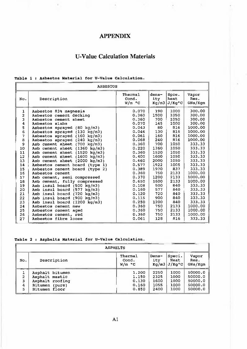
APPENDIX
U-Value Calculation Materials
Table 1 : Asbestos Material for U-Value Calculation.ASBESTOS
Thermal dens Spce. VaporNo. Description Cond. ity heat Res.
W/m °C Kg/m3 J/Kg°C GNs/Kgm1 Asbestos 83% magnesia 0.070 190 1000 300.002 Asbestos cement decking 0.360 1500 1050 300.003 Asbestos cement sheet 0.360 700 1050 300.004 Asbestos slabs 0.070 145 1000 300.005 Asbestos sprayed (80 kg/m3) 0.043 80 816 1000.006 Asbestos sprayed (130 kg/m3) 0.046 130 816 1000.007 Asbestos sprayed (160 kg/m3) 0.061 160 816 1000.008 Asbestos sprayed (240 kg/m3) 0.068 240 816 1000.009 Asb cement sheet (700 kg/m3) 0.360 700 1050 333.33
10 Asb cement sheet (1360 kg/m3) 0.220 1360 1050 333.3311 Asb cement sheet (1520 kg/m3) 0.360 1520 1050 333.3312 Asb cement sheet (1600 kg/m3) 0.400 1600 1050 333.3313 Asb cement sheet (2000 kg/m3) 0.660 2000 1050 333.3314 Asbestos cement board (type 1) 0.577 1922 1005 333.3315 Asbestos cement board (type 2) 0.389 1970 837 333.3316 Asbestos cement 0.360 750 2133 1000.0017 Asb cement, semi compressed 0.370 1200 2133 1000.0018 Asb cement, fully compressed 0.650 1600 2133 1000.0019 Asb insul board (500 kg/m3) 0.108 500 840 333.3320 Asb insul board (577 kg/m3) 0.160 577 840 333.3321 Asb insul board (720 kg/m3) 0.120 720 840 333.3322 Asb insul board (900 kg/m3) 0.115 900 840 333.3323 Asb insul board (1200 kg/m3) 0.250 1200 840 333.3324 Asbestos cement new 0.360 750 2133 1000.0025 Asbestos cement aged 0.360 750 2133 1000.0026 Asbestos cement, red 0.360 750 2133 1000.0027 Asbestos fibre loose 0.061 128 816 333.33
Table 2 : Asphelts Material for U-Value Calculation.ASPHELTS
Thermal Dens Speci. VaporNo. Description Cond. ity Heat Res.
W/m °C Kg/m3 J/Kg°C GNs/Kgm1 Asphalt bitumen 1.200 2250 1000 50000.02 Asphalt mastic 1.150 2325 1000 50000.03 Asphalt roofing 0.130 1600 1000 50000.04 Bitumen (pure) 0.160 1055 1000 50000.05 Bitumen floor 0.850 2400 1000 50000.0
A1

Table 3 : Blocks Material for U-Value Calculation.BLOCKS
Thermal Dens Speci. VaporNo. Description Cond. ity Heat Res.
W/m °C Kg/m3 J/Kg°C GNs/Kgm1 Concrete block (heavywt) 1.630 2300 1000 100.002 Concrete block (lightwt) 0.190 600 1000 30.003 Concrete block (mediumwt) 0. 510 1400 1000 50.004 Foamed slag conc block (950) 0.200 950 1060 35.425 Foamed slag conc block (1040) 0.317 1040 1050 77.086 Foamed slag conc block (2000) 0.600 2000 1050 177.087 Cellular block outer leaf 0.490 720 1069 35.008 Cellular block inner leaf 0.290 720 1069 35.009 Clinker concrete block hollow 0.505 865 1069 35.00
10 Clinker block solid inner leaf 0.645 1040 1058 77.0811 Clinker conc block (1050) 0.350 1050 1057 77.0812 Clinker conc block (1520) 0.600 1520 1059 77.0813 Pumice concrete block 0.300 1250 1060 77.0814 Dense gravel blk (2000 kg/m3) 1.100 2000 1050 177.0815 Dense gravel blk (2400 kg/m3) 1.750 2400 1042 177.0816 Pfa conc block (950 kg/m3) 0.200 950 1053 35.4217 Pfa conc block (1760 kg/m3) 0.500 1760 1063 77.0818 Exp clay conc blk (720 kg/m3) 0.200 720 1069 35.4219 Exp clay conc blk (1760 kg/m3) 0.600 1760 1063 77.0820 Aerated, air cured conc block 0.850 400 1100 35.4221 Aerated, a/clvd conc blk (400) 0.080 400 1100 35.4222 Aerated, a/clvd conc blk (800) 0.250 800 1063 35.42
Table 4 : Brick Material for U-Value Calculation.BRICK
Thermal Dens Speci. VaporNo. Description Cond. ity Heat Res.
W/m °C Kg/m3 J/Kg°C GNs/Kgm1 Alumin refactory brick 0.290 720 1000 100.002 Brickwork (external) 0.840 1700 800 50.003 Brickwork (internal) 0.620 1700 800 50.004 Silica brick 1.300 1900 1000 100.005 Brickwork 0.700 1700 800 41.676 Brickwork (1200 kg/m3) 0.310 1200 750 41.677 Brickwork (1400 kg/m3) 0.420 1400 750 41.678 Brickwork (1600 kg/m3) 0.540 1600 750 41.679 Brickwork (1800 kg/m3) 0.710 1800 750 41.67
10 Brickwork (2000 kg/m3) 0.920 2000 750 41.6711 Brickwork common (dry) 0.810 1760 800 41.6712 Brick common (1530 kg/m3) 0.650 1530 920 50.0013 Brick common (1750 kg/m3) 0.600 1750 920 41.6714 Brick common (1790 kg/m3) 0.720 1790 920 41.6715 Brick common (1826 kg/m3) 0.820 1826 753 41.67
Continue
A2

BRICK
No. DescriptionThermal Cond.
W/m °CDens
ityKg/m3
Speci.Heat
J/Kg°CVapor Res.
GNs/Kgm1617181920 21 2223242526272829303132333435363738394041424344454647484950
Brick common (1920 kg/m3) Brick common (2050 kg/m3) Brick common (2200 kg/m3) Brick red common (dry) Fletton brick Fletton common inner Fletton claywall outer Fletton common, frog up Fletton common inner Fletton cellular outer Fletton cellular inner Fletton facing, outer Diatomaceous earth brick
(1500 kg/m3) (2000 kg/m3) (2100 kg/m3) (2175 kg/m3)
Brick facing Brick facing Brick facing Brick facing London stock Brick engineering (2100 kg/m3) Brick engineering (2300 kg/m3) Sandlime brick (1530 kg/m3) Sandlime brick (1890 kg/m3) Sandlime brick, red Sandlime brick, white Brick wire cut red Brick fletton dark Brick fletton light Brick light buff Brick creamBrick white/light cream Brick glazed ivory Brick glazed white Brick purple Brick Stafford blue Brick yellow buff
0.720 0.880 0.800 0.810 0.550 0.700 0.810 0.930 0.670 0.900 0.600 1.020 0.141 0. 5001.330 0.700 0.830 0.450 0.800 1.000 0.650 1.340 1.613 0.6501.330 0.550 0.550 0.810 0.810 0.810 0.810 0.810 0.810 0.800 0.810
192020502200176017001760176017601760176017601760720
1500200021002175157521002300153018901920153020001700170017601760176017601760176021001760
795920920920920920920920920920920920920920920920920920920920920920920920920920920920920920920920920920920
41.67 41. 6741.6741.6741.6741.6741.6741.6741.67 41. 6741.6741.6741.6741.6741.6741.6741.6741.6741.6741.6750.0096.3596.3550.00 41. 6741.6741.6741.6741.6741.6741.6741.6741.6741.6741.67
Zable 5 : Concrete Material for U-Value Calculation.CONCRETE
Thermal Dens Speci. VaporNo. Description Cond. ity Heat Res.
W/m °C Kg/m3 J/Kg°C GNs/Kgm1 Aerated concrete slab 0.160 500 840 40.002 Cast concrete dense 1.400 2100 840 200.003 Cast concrete lightweight 0.380 1200 1000 40.004 Rendering 0.400 1200 1000 100.005 Screed 0.410 1200 840 100.006 275 R.C SLAB 1.400 2100 840 200.00
A3

Table 6 : Felt Material for U-Value Calculation.FELT
Thermal Dens Speci. VaporNo. Description Cond. ity Heat Res.
W/m °C Kg/m3 J/Kg°C GNs/Kgm1 Bitumenous felt (loose laid) 0.200 1000 1000 8000.002 Felt in bitumen 0.500 1500 1000 50000.03 Roofing felt 0.190 960 1000 4000.004 Sarking 0.200 1100 1000 4000.00
Table 7 : Flooring Material for U-Value Calculation.FLOORING
Thermal Dens Speci. VaporNo. Description Cond. ity Heat Res.
W/m °C Kg/m3 J/Kg°C GNs/Kgm1 Carpet (foam backed) 0.100 1000 1000 200.002 Carpet (wool) 0.055 160 1000 10.003 Cork tiles 0.085 540 1000 100.004 Felt underlay 0.065 270 1000 10.005 PVC flooring 0.220 1600 1000 1000.006 Rubber flooring 0.310 1600 1000 200.007 Rubber underlay 0.100 400 1000 200.008 Timber flooring 0.140 650 1200 60.009 Wood block 0.140 650 1200 60.00
Table 8 : General Concrete Material for U-Value Calculation.GENERAL CONCRETE
Thermal Dens Speci. VaporNo. Description Cond. ity Heat Res.
W/m °C Kg/m3 J/Kg°C GNs/Kgm1 Concrete 1:2:4 1.400 2360 1030 208.332 Concrete (400 kg/m3) 0.150 400 925 35.423 Concrete (600 kg/m3) 0.200 600 920 35.424 Concrete (800 kg/m3) 0.230 800 925 35.425 Concrete (1000 kg/m3) 0.300 1000 920 77.086 Concrete (1200 kg/m3) 0.380 1200 920 77.087 Concrete (1400 kg/m3) 0.510 1400 920 77.088 Concrete (1600 kg/m3) 0.660 1600 920 77.089 Concrete (1800 kg/m3) 0.870 1800 920 77.08
10 Concrete (2000 kg/m3) 1.130 2000 920 77.0811 Concrete (2200 kg/m3) 1.450 2200 920 77.0812 Concrete (2400 kg/m3) 1.830 2400 920 77.0813 Dense concrete (2000 kg/m3) 1.130 2000 1000 77.0814 Dense concrete (2100 kg/m3) 1.400 2100 840 77.0815 Dense concrete (2300 kg/m3) 1.100 2300 1070 77.0816 Concrete screed (1200 kg/m3) 0.410 1200 840 77.0817 Concrete screed (2100 kg/m3) 1.280 2100 1000 77.08
A4

Zable 9 : Insulations Material for U-Value Calculation.INSULATIONS
Thermal Dens Speci. VaporNo. Description Cond.
W/m °City
Kg/m3Heat
J/Kg°CRes.
GNs/Kgm1 Cork board 0.042 145 1800 100.002 Cork granules 0.046 115 1800 100.003 Glassfibre quilt 0.040 12 840 5.004 Mineral wool felt 0.039 50 1000 5.005 Mineral wool mat 0.036 130 1000 5.006 Perlite granules 0.042 65 1000 5.007 Phenolic board 0.038 30 1400 260.008 Polystyrene beads 0.030 25 1000 300.009 Polystyrene board 0.030 25 1000 1000.00
10 Polyurethane board 0.020 30 1000 60.0011 Polyurethane foam 0.026 30 1000 60.0012 Urea formaldehyde foam 0.032 15 1500 15.0013 Vermiculite granules 0.065 100 1000 15.0014 Glass fibre (12 kg/m3) 0.040 12 833 15.0015 Glass fibre (25 kg/m3) 0.035 25 1000 15.0016 Glasswool (24 kg/m3) 0.039 24 920 7.8117 Glasswool (200 kg/m3) 0.040 200 670 6.2518 Glass foamed 0.045 125 840 6.2519 Mineral wool, fill type 0.039 150 840 5.9920 Mineral wool board 0.048 240 1050 14.06
1 21 Strawboard 0.100 370 1000 62.5022 Polystyrene sheet (16 kg/m3) 0.040 16 1210 109.3823 Polystyrene sheet (32 kg/m3) 0.033 32 1210 385.4224 Polystyrene, exp, open cell 0.033 25 1200 348.9625 Polystyrene, exp, closed cell 0.033 25 1200 1000.0026 Polystyrene, expanded 0.030 140 1380 307.2927 Polyurethane, foamed 0.026 30 1260 312.5028 Polyurethane board 0.025 30 1400 510.4229 PVC, expanded 0.045 70 1000 208.3330 Urea formaldehyde, foamed 0.032 30 1500 22.4031 Woodwool slab (300 kg/m3) 0.067 300 1000 15.0032 Woodwool slab (400 kg/m3) 0.080 400 1000 26.0433 Woodwool slab (500 kg/m3) 0.100 500 1000 27.0834 Woodwool slab (800 kg/m3) 0.130 800 1000 27.0835 Cork 0.041 100 1800 10.0036 Cork granulated (115 kg/m3) 0.046 115 1000 104.1737 Cork granulated (120 kg/m3) 0.047 120 1800 78.1338 Cork granulated (130 kg/m3) 0.045 130 1760 78.1339 Cork board (100 kg/m3) 0.039 100 1800 26.0440 Cork board (130 kg/m3) 0.040 130 1800 62. 5041 Cork board (145 kg/m3) 0.042 145 1000 104.1742 Cork board (160 kg/m3) 0.046 160 1800 62.5043 Cork board (180 kg/m3) 0.045 180 1800 40.0044 Cork tile (145 kg/m3) 0.040 145 2207 75.0045 Cork tile (530 kg/m3) 0.084 530 1670 102.6046 Cork tile (540 kg/m3) 0.085 540 1000 130.2147 Af/armaflex 0.036 60 1380 8000.00
A5
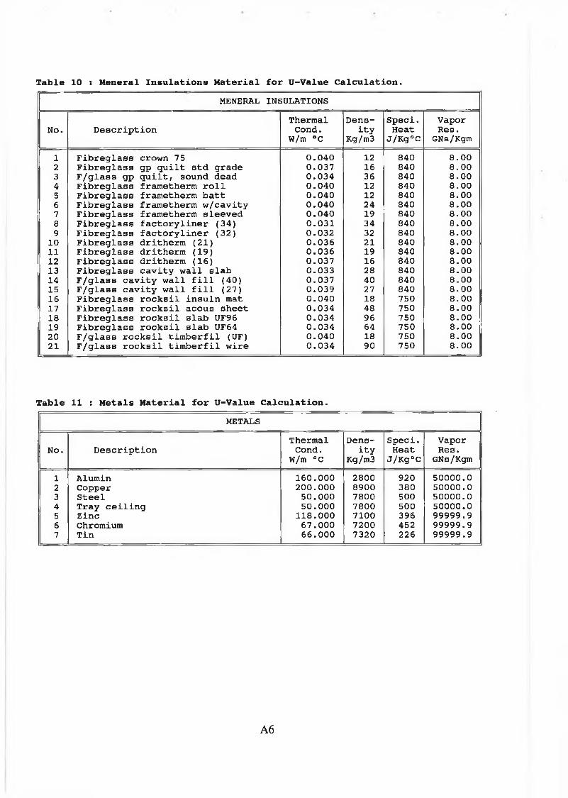
Table 10 : Menerai Insulations Material for U-Value Calculation.MENERAL INSULATIONS
Thermal Dens Speci. VaporNo. Description Cond. ity Heat Res.
W/m °C Kg/m3 J/Kg°c GNs/Kgm1 Fibreglass crown 75 0.040 12 840 8.002 Fibreglass gp quilt std grade 0.037 16 840 8.003 F/glass gp quilt, sound dead 0.034 36 840 8.004 Fibreglass frametherm roll 0.040 12 840 8.005 Fibreglass frametherm batt 0.040 12 840 8.006 Fibreglass frametherm w/cavity 0.040 24 840 8.007 Fibreglass frametherm sleeved 0.040 19 840 8.008 Fibreglass factoryliner (34) 0.031 34 840 8.009 Fibreglass factoryliner (32) 0.032 32 840 8.00
10 Fibreglass dritherm (21) 0.036 21 840 8.0011 Fibreglass dritherm (19) 0.036 19 840 8.0012 Fibreglass dritherm (16) 0.037 16 840 8.0013 Fibreglass cavity wall slab 0.033 28 840 8.0014 F/glass cavity wall fill (40) 0.037 40 840 8.0015 F/glass cavity wall fill (27) 0.039 27 840 8.0016 Fibreglass rocksil insuln mat 0.040 18 750 8.0017 Fibreglass rocksil acous sheet 0.034 48 750 8.0018 Fibreglass rocksil slab UF96 0.034 96 750 8.0019 Fibreglass rocksil slab UF64 0.034 64 750 8.0020 F/glass rocksil timberfil (UF) 0.040 18 750 8.0021 F/glass rocksil timberfil wire 0.034 90 750 8.00
Table 11 : Metals Material for U-Value Calculation.METALS
Thermal Dens Speci. VaporNo. Description Cond. ity Heat Res.
W/m °C Kg/m3 J/Kg°C GNs/Kgm1 Alumin 160.000 2800 920 50000.02 Copper 200.000 8900 380 50000.03 Steel 50.000 7800 500 50000.04 Tray ceiling 50.000 7800 500 50000.05 Zinc 118.000 7100 396 99999.96 Chromium 67.000 7200 452 99999.97 Tin 66.000 7320 226 99999.9
A6

Table 12 : Plaster Material for U-Value Calculation.PLASTER
Thermal Dens Speci. VaporNo. Description Cond. ity Heat Res.
W/m °C Kg/m3 J/Kg°C GNs/Kgm1 Plaster (denae) 0.560 1300 1000 60.002 Plaster (lightwt) 0.160 600 1000 60.003 Plaster - gypsum 0.380 1100 840 60.004 Plaster - perlite 0.080 400 840 60.005 Plaster - sand/cement 0.530 1570 1000 60.006 Plaster - vermiculite 0.260 800 840 60.007 Plasterboard - gypsum 0.160 950 840 60.008 Plasterboard - perlite 0.180 800 840 60.009 Perlite aggr plaster (400) 0.079 400 837 57.29
10 Perlite aggr plaster (610) 0.190 610 837 57.2911 Vermiculite aggr plaster (480) 0.140 480 837 57.2912 Vermiculite aggr plaster (720) 0.220 720 837 57.2913 Vermiculite aggr plaster (960) 0.300 960 837 57.2914 Gypsum/vermiculite bonding 0.218 658 837 57.2915 Gypsum/perlite browning 0.162 570 837 57.2916 Gypsum plaster/perlite aggr 0.220 720 1340 57.2917 Lightweight plaster (448) 0.115 448 837 57.2918 Lightweight plaster (600) 0.170 600 917 50.0019 Lightweight plaster (770) 0.201 770 837 57.2920 Lightweight plaster (900) 0.259 900 837 57.2921 Cement/sand aggr plaster(1570) 0.530 1570 837 104.1722 Cement/sand aggr plaster(1182) 0.720 1182 837 104.1723 Gypsum plaster/sand aggr(1862) 0.577 1862 837 31.2524 Gypsum plaster/sand aggr(1680) 0.810 1680 837 31.2525 Plaster (1200 kg/m3) 0.420 1200 837 57.2926 Plaster (1300 kg/m3) 0.500 1300 837 60.0027 Plaster (1440 kg/m3) 0.480 1440 837 57.2928 Plaster (1600 kg/m3) 0. 600 1600 837 57.2929 Lime cement plaster 0.420 1600 837 114.5830 Plasterboard 0.160 960 837 57.2931 Cement rendering/mortar (1300) 0.500 1300 769 100.0032 Cement rendering/mortar (1600) 1.153 1600 1000 114.5833 Cement rendering/mortar (1778) 1.180 1778 1000 114.5834 Cement rendering/mortar (1890) 1.730 1890 780 100.00
Table 13 : Roofing Components Material for U-Value Calculation.ROOFING COMPONENTS
Thermal Dens Speci. VaporNo. Description Cond. ity Heat Res.
W/m °C Kg/m3 J/Kg°C GNs/Kgm1 Asphalt (1600 kg/m3) 0.430 1600 1000 5208.332 Asphalt (1700 kg/m3) 0.500 1700 1000 5208.333 Asphalt, heavy 1.220 2240 1000 5208.334 Asphalt, 20% grit (1920 kg/m3) 0. 580 1920 1000 5208.335 Asphalt, 20% grit (2320 kg/m3) 1.150 2320 840 5208.336 Bitumen 0.160 1055 1000 4166.677 Roofing felt (960 kg/m3) 0.410 960 1000 6770.838 Concrete tiles, uncoloured 1.100 2100 837 177.089 Concrete tile, black 1.100 2100 837 177.08
10 Concrete tile, brown 1.100 2100 837 177.0811 Slate, grey 2.000 2700 753 250.0012 Slate, blue-green 2.000 2700 753 250.0013 Slate, silver-grey/light 2.000 2700 753 250.0014 Clay tile, red/brown 0.850 1900 586 72.92
A7

Table 14 : Sheeting Material for U-Value Calculation.SHEETING
Thermal Dens Speci. VaporNo. Description Cond. ity Heat Res.
W/m °C Kg/m3 J/Kg°C GNs/Kgm1 Chipboard 0.150 800 1000 500.002 Fibreboard 0.060 300 1400 40.003 Fire retardant boarding 0.100 800 1000 80.004 Glass hollow block 0.680 1000 830 50000.05 Glass sheet 1.050 2500 830 50000.06 Hardboard medium 0.080 600 2000 600.007 Hardboard standard 0.130 900 2000 600.008 PVC rigid sheet 0.160 1350 1250 1000.009 Polystyrene 0.030 25 1000 1000.00
10 Woodwool slab 0.100 500 1000 20.0011 Fibre board (240 kg/m3) 0.053 240 1400 20.0012 Fibre board (270 kg/m3) 0.049 270 1423 20.0013 Fibre board (290 kg/m3) 0.060 290 1420 20.0014 Fibre board (300 kg/m3) 0.060 300 1000 20.0015 Fibre board (300 kg/m3) 0.050 300 2335 40.0016 Fibre board (320 kg/m3) 0.059 320 1670 20.0017 Fibre board (350 kg/m3) 0.069 350 1400 20.0018 Fibre board (400 kg/m3) 0.060 400 1400 20.0019 Fibre board (480 kg/m3) 0.060 480 1400 20.0020 Fibre board (720 kg/m3) 0.090 720 1400 20.0021 Fibre board (800 kg/m3) 0.101 800 1400 20.0022 Fibre board (880 kg/m3) 0.144 880 1400 20.0023 Particle board low density 0.078 593 1300 20.0024 Particle board medium density 0.135 800 1300 20.0025 Particle board high density 0.170 1000 1300 20.0026 Hardboard 0.200 900 2444 598.9627 Hardboard (tempered) 0.180 960 2000 557.2928 Plywood (513 kg/m3) 0.124 513 2000 520.8329 Plywood (530 kg/m3) 0.140 530 2760 520.8330 Plywood (544 kg/m3) 0.115 544 1214 520.8331 Plywood (650 kg/m3) 0.140 650 2308 520.8332 Plywood (fireproofed) 0.150 560 2000 520.8333 Resin bonded plywood 0.140 650 2000 666.6734 Chip board (480 kg/m3) 0.110 480 1590 500.0035 Chip board (700 kg/m3) 0.110 700 1570 500.0036 Chip board (800 kg/m3) 0.150 800 2090 500.00
A8

Table 15 : Timber Material for U-Value Calculation.TIMBER
Thermal Dens Speci. VaporNo. Description Cond. ity Heat Res.
W/m °C Kg/m3 J/Kg°C GNs/Kgm1 Hardwood 0.150 700 1200 60.002 Mahogany 0.155 700 1200 60.003 Oak 0.160 770 1200 60.004 Pine 0.140 660 1200 500.005 Plywood 0.150 560 2800 1000.006 Softwood 0.130 500 2800 60.007 Teak 0.170 700 1200 60.008 Softwood (500 kg/m3) 0.140 500 1760 60.009 Softwood (630 kg/m3) 0.130 630 2760 59.48
10 Hardwood (650 kg/m3) 0.160 650 2300 60.0011 Hardwood (700 kg/m3) 0.150 700 1420 59.4812 Timber (12% moisture) 0.144 560 1420 59.4813 Timber (20% moisture) 0.144 480 1420 59.4814 Timber smooth planed 0.144 560 1420 59.4815 Wood 0.147 640 1420 59.4816 Beech, across grain, 15% 0.167 700 1420 187.5017 Cypress, across grain 0.097 465 1420 59.4818 Deal, across grain 12% 0.125 610 1420 59.4819 Deal, along grain 12% 0.220 610 1420 59.4820 Fir (513 kg/m3) 0.115 513 1380 59.4821 Fir (545 kg/m3) 0.115 545 2720 59.4822 Fir, across grain 0.109 420 2720 59.4823 Fir, along grain 0.138 420 2720 59.4824 Mahogany across grain 10% 0.156 700 1420 59.4825 Maple (720 kg/m3) 0.159 720 1256 59.4826 Maple (640 kg/m3) 0.173 640 1420 59.4827 Oak, radial (480 kg/m3) 0.173 480 2390 59.4828 Oak, radial (610 kg/m3) 0.207 610 2390 59.4829 Oak, across grain 0.166 545 2390 59.4830 Oak, across grain 14% 0.159 770 2390 59.4831 Oak, along grain 14% 0.290 770 2390 59.4832 Pine, white 0.112 500 2805 59.4833 Pine, yellow, across grain 0.147 640 2805 59.4834 Pine (15% moisture) 0.138 660 1420 59.4835 Spruce (12% moisture) 0.105 420 1420 59.4836 Teak (10% moisture) 0.138 720 1420 59.48
A9

Table 16: Vapor Barrieres Material for U-Value Calculation.VAPOR BARRIERES
No. Description Vapor Res. GNs/Kgm
1 Aluminium foil 4000.002 Building paper 5.003 Building paper, foil backed 4000.004 Insulation board painted 10.005 Insulation board emulsioned 2.006 Kraft paper 0.207 Plaster painted 8.008 Plasterboard foil backed 200.009 Plywood painted 8.00
10 Polythene (0.12 mm) 250.0011 Roofing felt 10.0012 Vinyl wallpaper 10.0013 Aluminium foil on paper 1000.0014 Alum foil bond to kraft paper 877.2015 PVC unplasticised .0051mm 257.1016 PVC plasticised .1mm 15.9017 Polythene 0.05mm 120.6018 Polythene 0.1mm 217.4019 Polythene 0.15mm 349.7020 Water proof paper 0.4021 Black building paper 103.1022 Laminated paper 42.0023 Paper, white 7.7024 Kraft paper, single 0.2025 Kraft paper, double 0.3026 Kraft paper, 3 ply 0.5027 Kraft paper, 4 ply 0.6028 Kraft paper, 5 ply 0.6029 Asphalt coated paper 50.0030 Asphalt infused sheath paper 2.7031 Bitumen impregnated paper 11.1032 Sheathing paper 7.7033 Waxed paper, medium weight 196.1034 Waxed paper, heavy weight 158.7035 Polyethylene 0.0508mm 109.3036 Polyethylene 0.102mm 218.3037 Polyethylene 0.152mm 291.5038 Polyethylene 0.203mm 436.7039 Polyethylene 0.254mm 581.4040 Gloss paint average 23.8041 Interior paints, various 1 ct 29.0042 Varnishes 0.05mm 5.0043 Accolade f/glass fissure face 22.0044 Roofing felt 10.0045 Felt + hot bitumen 52083.33
A10