Development of a Model andSimulation Framework

for a Modular Robotic Leg

Authored by

Katiegrace Youngsma

A Thesis

Submitted to the Faculty of

Worcester Polytechnic Institute

in partial fulfillment of the requirements for the

Degree of Master of Science

in

Robotics Engineering

June 11, 2012

Approved by:

Dr. Taskin Padir, Assistant Professor, Robotics Engineering Program

Dr. William Michalson, Professor, Robotics Engineering Program

Dr. Michael Gennert, Professor, Robotics Engineering Program

Abstract

As research in the field of mobile robotics continues to advance, legged robotsin different forms and shapes find a variety of applications on rough terrainwhere wheeled robots fail to operate in practice. For this reason, a modularlegged robot platform is being developed at WPI. This research focuses ondeveloping a mathematical model and then building a simulation to verify themodel for a single leg for this platform. The robot platform is modular in thesense that leg modules can be removed and added to predetermined ports onthe robot chassis. The modularity of a legged robot is a significant advance-ment in mobile robotics technology as it enables a single robot to take ondifferent body configurations depending on circumstances and environmentto achieve its goals. It also poses a challenge in terms of overall design as itrequires autonomous operation of the leg. The goal for this research is to inpart fulfill the need for a mathematical model for an autonomous leg. Thisresearch investigates the development of a kinematic and dynamic model forthe leg, a step trajectory for walking, a simulation of the system to verify thedynamic model, and various functions and scripts to identify shortcomingswithin the model. This research uses Mathworks Matlab and Wolfram Math-ematica to develop the mathematical model, and Matlab Simulink SimMe-chanics and Matlab functions to build a simulation. Both the mathematicalmodel and simulation follow the classic design of other legged robots, utiliz-ing Lagrangian dynamics, the Jacobian, and simulation tools. The result isa project that is unique in that it drives a robot leg almost independentlywith very limited communication to a central controller.

Contents

1 Introduction 11.1 Purpose . . . . . . . . . . . . . . . . . . . . . . . . . . . . . . 11.2 Report Overview . . . . . . . . . . . . . . . . . . . . . . . . . 21.3 Background . . . . . . . . . . . . . . . . . . . . . . . . . . . . 31.4 Accomplishments . . . . . . . . . . . . . . . . . . . . . . . . . 10

2 Kinematic and Dynamic Modeling of a Robot Leg 122.1 Mechanical Design . . . . . . . . . . . . . . . . . . . . . . . . 122.2 Forward Kinematics . . . . . . . . . . . . . . . . . . . . . . . 182.3 SimMechanics Model . . . . . . . . . . . . . . . . . . . . . . . 202.4 Inverse Kinematics . . . . . . . . . . . . . . . . . . . . . . . . 252.5 The Full Robot Body . . . . . . . . . . . . . . . . . . . . . . . 262.6 Chapter 2 Summary . . . . . . . . . . . . . . . . . . . . . . . 27

3 Robot Leg Dynamics 283.1 Calculating the Jacobian Matrix . . . . . . . . . . . . . . . . . 283.2 Dynamics . . . . . . . . . . . . . . . . . . . . . . . . . . . . . 30

3.2.1 Components of the Manipulator Lagrangian . . . . . . 313.2.2 Methods of Computing the Euler-Lagrange for a Ma-

nipulator . . . . . . . . . . . . . . . . . . . . . . . . . . 333.3 Using User Defined Blocks . . . . . . . . . . . . . . . . . . . . 373.4 Chapter 3 Summary . . . . . . . . . . . . . . . . . . . . . . . 37

4 Simulating the Leg 384.1 Leg Trajectory . . . . . . . . . . . . . . . . . . . . . . . . . . 40

4.1.1 Workspace . . . . . . . . . . . . . . . . . . . . . . . . . 404.1.2 Set Points . . . . . . . . . . . . . . . . . . . . . . . . . 414.1.3 Generating Smooth Trajectories . . . . . . . . . . . . . 434.1.4 Trajectory Generation Methods in the Simulation . . . 454.1.5 Stability Polygon . . . . . . . . . . . . . . . . . . . . . 474.1.6 Checking for Singularities and Manipulability . . . . . 48

i

4.1.7 Derivatives of Time Step Functions in Simulink . . . . 494.2 User Defined Blocks . . . . . . . . . . . . . . . . . . . . . . . 534.3 Verifying the Simulink Model . . . . . . . . . . . . . . . . . . 53

5 Conclusions and Future Work 565.1 Results . . . . . . . . . . . . . . . . . . . . . . . . . . . . . . . 56

5.1.1 Simulation Result Analysis . . . . . . . . . . . . . . . . 565.2 Inverting the Model . . . . . . . . . . . . . . . . . . . . . . . . 56

5.2.1 Matlab . . . . . . . . . . . . . . . . . . . . . . . . . . . 585.3 Future Work . . . . . . . . . . . . . . . . . . . . . . . . . . . . 60

5.3.1 PID or PD Control . . . . . . . . . . . . . . . . . . . . 605.3.2 Using the Leg as a Manipulator . . . . . . . . . . . . . 615.3.3 Step Planning . . . . . . . . . . . . . . . . . . . . . . . 625.3.4 Central Processing . . . . . . . . . . . . . . . . . . . . 625.3.5 Universal Modules . . . . . . . . . . . . . . . . . . . . 63

A Appendix A: Mathematica Script 66

B Appendix B: Symbolic Matlab Scripts 72

C Appendix C: Matlab Files for ode45 Solver and Singular-ity/Manipulability Check 75

ii

Chapter 1

Introduction

1.1 Purpose

Every robot, every being, has a purpose for its existence. The motivation fora reconfigurable robot, is that for every purpose, there will be a configurationwhich the robot can take on to accomplish that purpose. The proposed solu-tion is a robot where the sensors, the actuators, and the processing dedicatedto each peripheral are modular. Meaning each part is simply an attachmentthat can be used or removed on the robot to suit its mission and environment.This project is a part of the process of developing a fully functioning recon-figurable multi-legged robot. This is a significant development because, inprevious developments research investigated legged walking for robots whichwere fully defined. Meaning basic parameters such as the number of legs,size, overall mass, and which sensors were available were known. Howeverthis robot is, by its nature, physically undefined until it is placed togetherin its desired configuration. This robot could potentially take on configura-tions that would enable it to accomplish a wide variety of tasks. While thisresearch focuses on designing a leg to enable the robot to walk, there is noreason why it could not have wheel modules instead, giving it the ability tonavigate over flat surfaces very quickly. One could even place wheels on theend of legs, making it a wheeled robot of variable height and able to lift itswheels over obstacles. The reconfigurable robot being developed at WPI has12 multi-use ports for attachments which have yet to be designed, but has awide range of possible applications.

The reconfigurable robot has been designed such that the central bodyfor the robot would simply act as a physical frame on which to bolt the com-ponents, a power bus for the modules (since the power supplies themselvesshould also be modular, allowing the user to balance the weight to stored

1

energy ratio for a given mission), and an information bus for data that needsto be shared among the modules. The ports could be used for a variety ofsensors, as simple or as advanced as the robot needs to accomplish its pur-pose. For basic navigation something as inexpensive or lightweight as a sonarrange finder could be used, however for outdoor navigation through rubblesomething more advanced like a video array may be required. Either onecan be mounted provided it can attach to the universal ports on the robotbody. This particular robot design seeks to move the central processing outto its modular attachments, so that the body is not weighed down with acomplicated controller. This is ideal since different type and grades of sen-sors require varying amounts of processing. On this robot, the sensor anddedicated sensor processing would be handled on the peripheral attachment,such that it only sends useful information through the robot body. The goalfor this particular research is to model and simulate a single leg for reconfig-urable robot. Specifically to design a modular leg with its own processing andcontrol that needs minimal communication with the robot body to achievestable walking.

1.2 Report Overview

This paper has been introduced with an explanation of the purpose andneed for a primarily autonomous leg for a reconfigurable robot. The reportthen discusses the history of advances in legged mechanisms, legged robots,and reconfigurable robots. This includes a short literature review of paperspresented by those whose study has contributed to the work done in thisproject. We then discuss the overall design and construction of the robotleg. Beginning with a proposed mechanical design, and a discussion of howto physically model the leg using Matlab’s Simulink software with the Sim-Mechanics package. This section also guides the reader through the forwardand inverse kinematics for this robot leg, using the mathematical techniquesoutlined in the textbook, “Robot Modeling and Control” [1]. The third sec-tion continues the mathematical model and demonstrates calculations forthe Jacobian and Euler-Lagrange dynamics for the single robot leg. Section4 discusses the leg as simulated in the Simulink software. It begins with alengthy discussion on how to generate the trajectory for a single robot legand compares two different methods. It then discusses the details of the con-struction and flow of the Simulink simulation: how the mathematical modeloutlined in Section 3 is incorporated into the simulation, how the trajectoryfeeds into the system, and how these components interface with the Sim-Mechanics physical model. It then discusses how the simulation is used to

2

analyze verify the mathematical model. Section 5 discusses the results ofthe data collected from the simulation and identifies ways to define errorsthat came up in the results from the simulation. This section later describesfuture work that could be conducted with this project. The discussion onfuture work goes as far to propose ideas for the full operating reconfigurablerobot.

1.3 Background

Many technological advancements utilize wheels to achieve faster and moreenergy efficient mobility, however, soon after their development man musthave realized that only creatures with legs could properly navigate over dra-matically uneven terrain, the way an ant navigates thick grass or a mulenavigates a canyon. Only legged beings could step over objects and maintainstability on surfaces with varying heights. These scenarios demonstrate somemotivation for legged robots as opposed to those on wheels or tracks.

Ideas for mechanical walking creatures may go back as far as 480 BC, andmany images and ideas for various artificial animals can be found throughoutthe centuries [2]. The first real documented attempt for a walking machineare concepts for basic linkage driven machines. In 1893, Rigg took out apatent for a mechanical horse, proving that although legged mobility wasavailable through domestic animals, a machine that could accomplish thesame task was desired [3]. The first documented designs for a walking robotsarrive in the 1970’s, with WABOT 1, a statically stable robot developed byI. Kato, and an active exoskeleton developed independently by M. Vukobra-tovic. Vukobratovic’s work was not statically stable, but rather developedthe concept of the Zero Moment Point (ZMP) for dynamic walking. Thiswork inspired the need for research in dynamics of mobile legged robots.[4].

While investigating ideas to support this project, a wide variety of pa-pers and concepts were reviewed [4] [5] [6] [7] [8] [9] [10] [11] [12] [13]. Asmentioned, Vukobratovic developed the idea of the ZMP control method fordynamic walking. The ZMP method involves taking readings from force sen-sors placed on the legged robot’s feet. By measuring the reaction forces onthe “ground”, the controller calculates the zero-moment point.

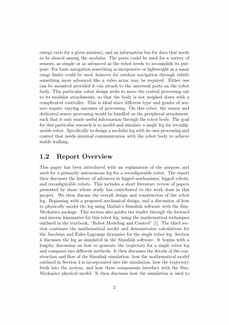
It is named thus since it is the single point around which no force is gen-erating a moment on the robot. That is, the sum of all the moments on therobot body (gravity, reaction forces, etc.) sum to zero at this point (See Fig-ure 1.1). To maintain stability, this point must lie within the robot’s supportpolygon for dynamically stable movement. Using Newtonian dynamics, onecan predict the location of the ZMP based on expected movement. In Vuko-

3

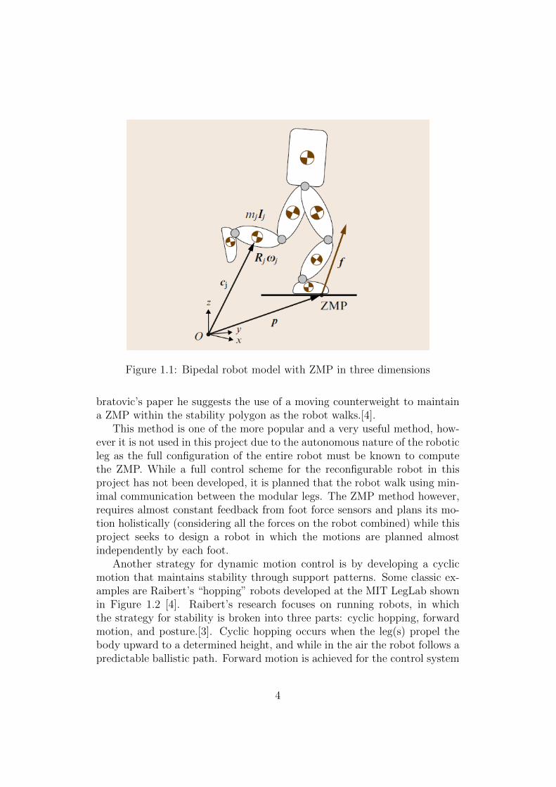
Figure 1.1: Bipedal robot model with ZMP in three dimensions

bratovic’s paper he suggests the use of a moving counterweight to maintaina ZMP within the stability polygon as the robot walks.[4].

This method is one of the more popular and a very useful method, how-ever it is not used in this project due to the autonomous nature of the roboticleg as the full configuration of the entire robot must be known to computethe ZMP. While a full control scheme for the reconfigurable robot in thisproject has not been developed, it is planned that the robot walk using min-imal communication between the modular legs. The ZMP method however,requires almost constant feedback from foot force sensors and plans its mo-tion holistically (considering all the forces on the robot combined) while thisproject seeks to design a robot in which the motions are planned almostindependently by each foot.

Another strategy for dynamic motion control is by developing a cyclicmotion that maintains stability through support patterns. Some classic ex-amples are Raibert’s “hopping” robots developed at the MIT LegLab shownin Figure 1.2 [4]. Raibert’s research focuses on running robots, in whichthe strategy for stability is broken into three parts: cyclic hopping, forwardmotion, and posture.[3]. Cyclic hopping occurs when the leg(s) propel thebody upward to a determined height, and while in the air the robot follows apredictable ballistic path. Forward motion is achieved for the control system

4

by moving the foot or feet to a desired position while the robot is in theair, such that when the robot lands it will be propelled forward in the nextbounce. Posture is the angles at which the foot or feet need to be locatedto maintain stability in three dimensional space over the given terrain. Themethod is not used for this project because it is specifically designed forrunning robots, which at this time the goal for this robot is stable walking.

Figure 1.2: The MIT LegLab’s Dynamically Stable “hopping” robots

This project instead uses a more basic strategy for stability, and that is bymaintaining its center of mass well within its stability polygon such that it isstatically stable, and keeping dynamic forces from the legs to a minimum toavoid upsetting the balance. Should further developments to this robot arisethat require the legs to move quickly and thus exert more dynamic forces onthe body, a more advanced control system like those described above wouldneed to be developed.

One control development that is very useful for this project is that ofadaptive locomotion over uneven terrain as described by McGhee and Iswandhi[10]. McGhee and Iswandhi describe how adaptive locomotion can be realizedby developing a sequence of support states as the robot steps over uneventerrain. It describes how the robot may optimally place its steps to avoidinterference with other legs, move within its reachable area, and maintainstability of the robot body.[10]. It stresses the importance of maintaining asupport pattern for the robot’s center of mass throughout all stages of thewalking pattern. This study was considered for this project while developing

5

the leg trajectories. Later we will show how a Matlab script was developed todemonstrate that the robot center of mass (CoM) remains within its supportpolygon throughout the leg step trajectory. When McGhee’s robot walksin an adaptive manner (meaning the leg trajectory changes) an algorithmdetermines what “cells” or areas of space are acceptable for leg placement tomaintain stability.

Waldron and McGhee later develop an adaptive walking hexapod robot.Waldron is known for exploring motion and force management for eachrobotic leg as it interacts with the ground on a robot with quasi-static sta-bility [14]. Waldron’s methods were not explored in depth for this projectsince they deal primarily with balancing overall robot forces to avoid slip.Since we use the Lagrangian to determine the necessary joint torques toachieve desired forces for the robot feet, further equations for balancing theforces should not be necessary. Instead, the torques provided by joint motorsare specifically specified to maintain the desired leg position throughout thestepping trajectory.

In 1992, Boissonnat, Devillers, Preperata, and Donati outlined properwalking patterns for their own spider robot. This group set out their ownalgorithms for robot foot placement while insuring the robot maintains astable configuration [6]. This method is almost identical to that used byMcGhee to determine areas that are acceptable for foot placement, only thatBoissonnat uses sets and unions to determine or eliminate areas in which therobot could step. Once again, for this project we use a single cyclic trajectorywhich repeats for each step. However it would be of great benefit to be ableto adapt the trajectory using the methods of either McGhee or Boissonnat[10] [6]. Kimura, Maufroy, and Takase also expand upon the ideas of McGheeand Iswandi to develop a robot with adaptive walking using a very differentstrategy that is more appealing for rough terrain. Rather than adjustingwhere the robot’s foot can be placed, Maufroy focuses on when the stepcycle for the robotic steps can be broken. For example, if there were a rockon the ground, McGhee or Boissonnat’s method would make an effort to notstep in that area, whereas Kimura’s former robot would merely rest its footatop the rock and end the step cycle there. [9][10]. What makes Maufroy’smethod possible is the addition of some kind of sensor on the robot foot.

Kimura also developed a robot for dynamic walking with Fukuoka andCohen called Tekken 2. Tekken 2 uses similar gait and walking conceptsto that developed with Maufroy, utilizing a step cycle. However the legmechanical design utilizes springs such that its gait is more like the hoppingmotion of Raibert’s robots than those of McGhee’s hexapod [8]. Anothermajor difference of note between the hexapods of McGhee and Waldron andthe quadrupeds of Kimura and Maufroy is the overall construction of the leg.

6

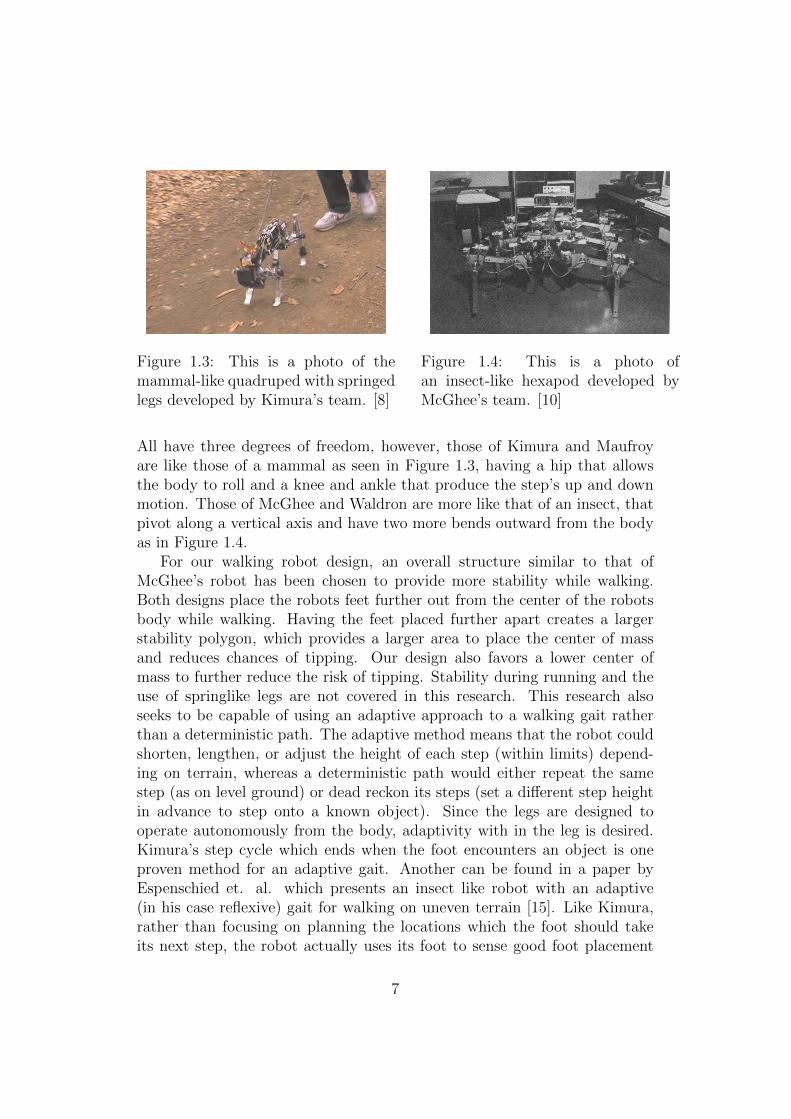
Figure 1.3: This is a photo of themammal-like quadruped with springedlegs developed by Kimura’s team. [8]

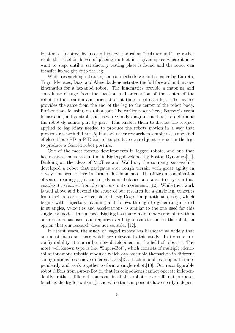
Figure 1.4: This is a photo ofan insect-like hexapod developed byMcGhee’s team. [10]

All have three degrees of freedom, however, those of Kimura and Maufroyare like those of a mammal as seen in Figure 1.3, having a hip that allowsthe body to roll and a knee and ankle that produce the step’s up and downmotion. Those of McGhee and Waldron are more like that of an insect, thatpivot along a vertical axis and have two more bends outward from the bodyas in Figure 1.4.

For our walking robot design, an overall structure similar to that ofMcGhee’s robot has been chosen to provide more stability while walking.Both designs place the robots feet further out from the center of the robotsbody while walking. Having the feet placed further apart creates a largerstability polygon, which provides a larger area to place the center of massand reduces chances of tipping. Our design also favors a lower center ofmass to further reduce the risk of tipping. Stability during running and theuse of springlike legs are not covered in this research. This research alsoseeks to be capable of using an adaptive approach to a walking gait ratherthan a deterministic path. The adaptive method means that the robot couldshorten, lengthen, or adjust the height of each step (within limits) depend-ing on terrain, whereas a deterministic path would either repeat the samestep (as on level ground) or dead reckon its steps (set a different step heightin advance to step onto a known object). Since the legs are designed tooperate autonomously from the body, adaptivity with in the leg is desired.Kimura’s step cycle which ends when the foot encounters an object is oneproven method for an adaptive gait. Another can be found in a paper byEspenschied et. al. which presents an insect like robot with an adaptive(in his case reflexive) gait for walking on uneven terrain [15]. Like Kimura,rather than focusing on planning the locations which the foot should takeits next step, the robot actually uses its foot to sense good foot placement

7

locations. Inspired by insects biology, the robot “feels around”, or ratherreads the reaction forces of placing its foot in a given space where it maywant to step, until a satisfactory resting place is found and the robot cantransfer its weight onto the leg.

While researching robot leg control methods we find a paper by Barreto,Trigo, Menezes, Diaz, and Almeida demonstrates the full forward and inversekinematics for a hexapod robot. The kinematics provide a mapping andcoordinate change from the location and orientation of the center of therobot to the location and orientation at the end of each leg. The inverseprovides the same from the end of the leg to the center of the robot body.Rather than focusing on robot gait like earlier researchers, Barreto’s teamfocuses on joint control, and uses free-body diagram methods to determinethe robot dynamics part by part. This enables them to discuss the torquesapplied to leg joints needed to produce the robots motion in a way thatprevious research did not.[5] Instead, other researchers simply use some kindof closed loop PD or PID control to produce desired joint torques in the legsto produce a desired robot posture.

One of the most famous developments in legged robots, and one thathas received much recognition is BigDog developed by Boston Dynamics[12].Building on the ideas of McGhee and Waldron, the company successfullydeveloped a robot that navigates over rough terrain with great agility ina way not seen before in former developments. It utilizes a combinationof sensor readings, gait control, dynamic balance, and a control system thatenables it to recover from disruptions in its movement. [12]. While their workis well above and beyond the scope of our research for a single leg, conceptsfrom their research were considered. Big Dog’s computational design, whichbegins with trajectory planning and follows through to generating desiredjoint angles, velocities and accelerations, is similar to the one used for thissingle leg model. In contrast, BigDog has many more modes and states thanour research has used, and requires over fifty sensors to control the robot, anoption that our research does not consider [12].

In recent years, the study of legged robots has branched so widely thatone must focus on those which are relevant to this study. In terms of re-configurability, it is a rather new development in the field of robotics. Themost well known type is like “Super-Bot”, which consists of multiple identi-cal autonomous robotic modules which can assemble themselves in differentconfigurations to achieve different tasks[13]. Each module can operate inde-pendently and work together to form a single robot.[13]. Our reconfigurablerobot differs from Super-Bot in that its components cannot operate indepen-dently; rather, different components of this robot serve different purposes(such as the leg for walking), and while the components have nearly indepen-

8

dent control, they will not function unless manually attached to the centralrobot body. In this sense, our reconfigurable robot design is more like thatof MiniQuad shown in Figure 1.5[7], which has body section modules so theuser can change the number of legs on the robot. We will also briefly presenta mechanical design for a multi-legged robot, which uses a compacted versionof the architecture used by McGhee. MiniQuad’s developers also outline thecontrol scheme for the robot. Using a tiered control approach, they use afull computer as a master controller, a “body level controller” to determinegait and foot position, and individual unit controllers for each actuator andsensor.

The robot design presented in here is reconfigurable in the sense that ithas a body with multiple ports, each of which is universal so that a manipula-tor or sensor can be attached. With this advantage, one can add capabilitiesto the robot for specific missions, or remove extraneous components to reduceweight for others. In this paper, we will take the term reconfigurable to meanthat components of the robot can be removed and added without inhibitingthe operability of the robot as a whole. Specifically, we focus on a leg asa module that could be added or removed from a robot while maintainingoverall operability, and so long that there are more than four legs, the robotis able to walk. The reconfigurable robot model presented in this paper andshown in Figure 1.6 will build off the reconfigurable robot platform previouslydeveloped at WPI which sought to develop a robot body with 12 ports forattachable legs each with an independent controller on each. The platformwas presented at the 2010 ICRA Workshop by Professor Taskin Padir andstudents as their Major Qualifying Project (MQP). [16]

Figure 1.5: This is a photo of Mini-Quad, a modular robot with insect-likelegs designed by Chen [7]

Figure 1.6: This is a rendering ofthe mechanical design previously de-veloped for this research [16]

9

In order to achieve this goal, we develop the necessary kinematics anddynamics as outlined by Spong in his book, Robot Modeling and Control [1].The design is then verified using a software program with knowledge of therobot’s construction. In 1990, Micheal McKenna and David Zeltzer presenta paper on Dynamic Simulation of Autonomous Legged Locomotion. Similarto this study, McKenna and Zeltzer use a software package which uses itsknowledge of the robot kinematics and dynamics to complete this simulation.Zeltzer developed a gait controller for their hexapod robot influenced by thework of McGhee. However, to determine necessary joint torques to supportthe robot body and achieve desired leg configurations, they use a programcalled Corpus. Their program consists of a dynamic simulator, gait controller,and motor programs. The dynamic simulator forms the base of the simulationand utilizes the gait program to determine desired joint positions, and themotor programs to deliver forces to the joints.[11]

This research utilizes the SimMechanics toolbox for MathWorks’s Simulinkis a valuable tool for all kinds of physical system modeling. Systems are mod-eled using a series of what Simulink calls “blocks” linked to one another viainputs and outputs, like a breadboard of electrical components with wirescarrying various kinds of signals. The wires are fairly universal, howevereach block needs to be set up with various parameters to do what the userdesires it to do. Blocks include those that do mathematical computations,signal processing, and with the SimMechanics package, act as physical bod-ies. After setting various block parameters as joint configurations, physicalinformation about bodies and joints, and environmental information, one canmodel any physical system imaginable. However, a shortcoming arises whentime step dependent input signals are needed. Simulink provides blocks forvarious mathematical signals, such as sine waves and transfer functions, how-ever for products of polynomial and advanced functions (such as those in thisproject used to generate joint torques over the course of the step trajectory)one must first write them in Matlab and then interface them with the rest ofthe system. In robotics, where complex and novel trajectories are frequentlyused, this can be a challenge. This research also seeks to show methods ofintegrating such signals into a SimMechanics simulation.

1.4 Accomplishments

Here is a short bulleted list highlighting the goals accomplished in this re-search.

• Full forward and inverse kinematics for the robotic leg

10

• Forward and inverse kinematics from the center of the robot body tothe end of each leg

• A Matlab script which displays a stick model of leg on the robot body

• Scripts to allow the static stability polygon and the robots center ofmass projected on the polygon

• A revised mechanical design for the robot leg

• The full Jacobian for the three degree of freedom leg

• Euler-Lagrange dynamic equations for the robot leg

• Three different Matlab scripts for leg trajectories

• Development of two methods for executing a quintic trajectory in Sim-Mechanics

• Sim-Mechanics model of the robotic leg

• A Simulink block which generates desired joint position, velocity, andacceleration for each leg trajectory

• A Simulink block which uses the Jacobian to translate forces exertedon the robot foot to the joint torques necessary to overcome that force

• A Simulink/Sim-Mechanics model which uses the trajectory as an inputand returns the necessary joint torques

• A Simulink/Sim-Mechanics model which takes joint torques as an inputand returns the joint motion

• A Matlab function which calculates the Euler-Lagrange equations inmatrix form

• A Matlab function which returns a set of torques based on a trajectoryloop

• A Matlab script which uses ode45 to determine joint velocity and ac-celeration based on torques

• Calculation of leg singularities and manipulability throughout the mo-tion of the leg

11

Chapter 2

Kinematic and DynamicModeling of a Robot Leg

The primary focus and scope for this project is to fulfill the need for adynamic model of a single leg for the multi-legged reconfigurable robot as itsteps in such a way to move a full robot body forward. This paper does notinvestigate the scope of how the entire reconfigurable robot works together orthe design of its central processor. This project will outline the developmentof a trajectory for a general step motion for the leg which could be madeadaptive in future work.

2.1 Mechanical Design

The mechanical leg seeks to keep the leg as light and compact as possiblewhile containing leg components (such as motors and sensors) inside of theleg frame. We took the design for the original leg for this project and adaptedto achieve these goals. Both the former and newer designs placed motors andpotentiometers between rails and terminating each leg link with a gearbox tore-direct the motors force along the joint. Both designs are also influencedby MiniQuad 1 [7] in their construction and reconfigurability.

However, the old design was found lacking in its rigidity. When handingthe constructed robot leg one could feel a lot of slack in its joints, and thegearboxes were unlikely to hold during regular motion. It had nearly 10 inchlong legs made with one eighth inch aluminum rail on each side. The legshad gear boxes at each end made from blocks aluminum stock that wereapproximately 2 inch wide by 3 inch long and 1 inch deep with a small oneinch by 1 and a half inch area milled out to contain the gears. This resultedin light legs that were heavy and bulky at either end. The gears themselves

12

were too small (about half inch in diameter) to endure the forces appliedto them if the robot were to walk under load. Also, the gear shafts werecoupled to the motors with two shafts joined by a coupler that resided inanother milled out area of the aluminum block. Holding two leg links, onecould move the joint without the motors moving because of the slack in thecoupling. Also the coupled gears would often “skip”, that is disengage farenough such that torque could not transfer from one to the other. Figures ofthe original leg are shown in 2.1 and 2.2.

Figure 2.1: Former Leg Design

Figure 2.2: Former Hip Joint Design

A revised design for the robotic leg would require the following:1. The robot leg shall utilize the same motors and potentiometers imple-

mented in the previous design.

13

2. The robot legs shall be able to support the dynamic forces exerted bythe robot whole when at least four legs are used.

3. The robot leg links shall have sufficient length to allow it to step ontoor over objects.

4. The robot leg shall be free of objects that stick out to avoid gettingcaught on objects or limiting the range of motion.

5. The joint motors on the robot leg shall be able to provide torque tojoints without loss of motion (no skipping or slipping).

6. The potentiometers shall accurately read the position of the robotjoints by some direct factor of the actual joint position in radians.

The new robot design achieves these goals in the following ways:1. Motors and potentiometers were accurately measured and included in

the new model assembly to ensure fit.2. This has not been tested, but the new design has more supports and

less room for flex than the previous model.3. While the leg links are shorter than the previous model, they are still

capable of reaching up to 20 cm above and 40 cm below the robot body attheir extremes.

4. Potentiometers have been moved closer to links 2 and 3, and inside oflink 1 while they were previously on standoffs up to 2 cm from the legs. Themotors for link 2 and 3 still reside inside of link 2, and the motor for link 1has been moved partially inside the link where it was previously on standoffsabove the link.

5. Couplings have been eliminated from the shafts reduce change of slip-ping, and larger gears for joint 2 and 3 were used to reduce risk of skipping.

6. The potentiometers are now linked to the geartrain with a singlecoupler rather than two to reduce risk of slipping.

This design started by creating accurate CAD models of the originalmotors and potentiometers to be used in the final leg assembly. For thesecond requirement, the legs were made more robust by adding more bracingin the leg frame to avoid collapse. The length of the robot leg was actuallyshortened to provide the robot with more stability, however they are stillsufficiently long to step onto or over small objects. The former design alsoleft the motor and potentiometer for the first link sticking up and out from theleg.The re-designed robot leg frames place the motors inside the leg frame,with the potentiometers mounted flush with the edges of the frame. Thiskeeps the objects from sticking out from the robot leg. The issue of gearslop and skipping can be avoided by either using stronger boxes to containthe gears, or simply using larger gears with deeper teeth. The latter waschosen for simplicity and cost. In order to avoid adding further weight andvolume to the size of the boxes with the introduction or larger gears, the

14

gearboxes were re-designed to be smaller and fit more snugly into the legrails. To reduce extraneous length to the legs (thus reducing strain on thegears and motors) the motors were placed side by each inside the rails. Also,motors were attached to gears with long shafts and a number of couplings,which introduces slop through potential bending or twisting in the shaftsand couplings. The new design brought the motor closer to the gears, thusbringing the motor and potentiometer closer to the gears themselves andreducing shaft length and the number of couplings. By moving the motorsand potentiometers closer to the gears and joints, one can keep the legsfrom having items that stick out, as well as reduce bending, twisting, andskipping that may occur between the legs actual motion and its motors andpotentiometers, making the system as a whole more accurate.

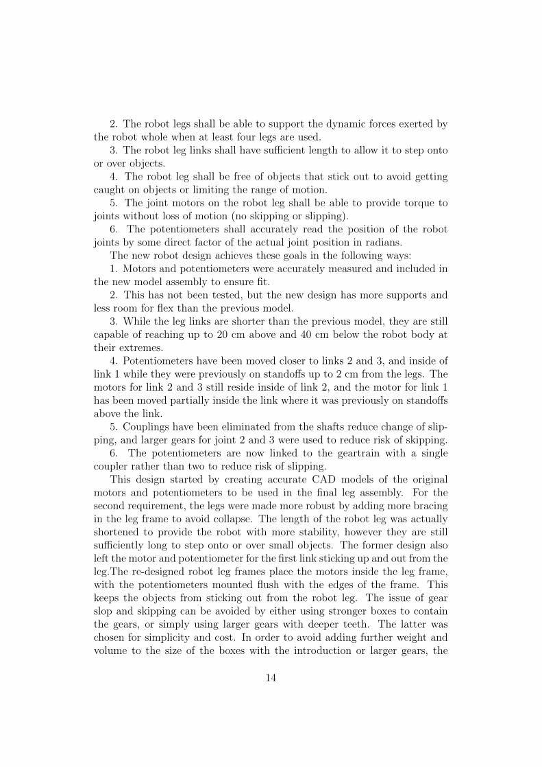
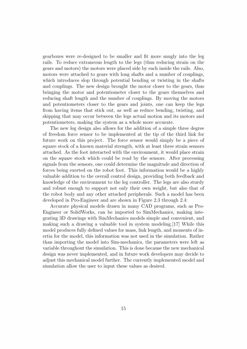
The new leg design also allows for the addition of a simple three degreeof freedom force sensor to be implemented at the tip of the third link forfuture work on this project. The force sensor would simply be a piece ofsquare stock of a known material strength, with at least three strain sensorsattached. As the foot interacted with the environment, it would place strainon the square stock which could be read by the sensors. After processingsignals from the sensors, one could determine the magnitude and direction offorces being exerted on the robot foot. This information would be a highlyvaluable addition to the overall control design, providing both feedback andknowledge of the environment to the leg controller. The legs are also sturdyand robust enough to support not only their own weight, but also that ofthe robot body and any other attached peripherals. Such a model has beendeveloped in Pro-Engineer and are shown in Figure 2.3 through 2.4:

Accurate physical models drawn in many CAD programs, such as Pro-Engineer or SolidWorks, can be imported to SimMechanics, making inte-grating 3D drawings with SimMechanics models simple and convenient, andmaking such a drawing a valuable tool in system modeling.[17] While thismodel produces fully defined values for mass, link length, and moments of in-ertia for the model, this information was not used in the simulation. Ratherthan importing the model into Sim-mechanics, the parameters were left asvariable throughout the simulation. This is done because the new mechanicaldesign was never implemented, and in future work developers may decide toadjust this mechanical model further. The currently implemented model andsimulation allow the user to input these values as desired.

15

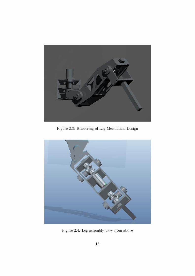
Figure 2.3: Rendering of Leg Mechanical Design

Figure 2.4: Leg assembly view from above

16

Figure 2.5: Leg assembly view from underneath

17

2.2 Forward Kinematics

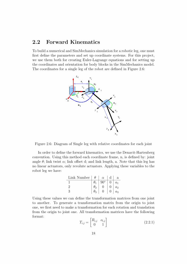
To build a numerical and SimMechanics simulation for a robotic leg, one mustfirst define the parameters and set up coordinate systems. For this project,we use them both for creating Euler-Lagrange equations and for setting upthe coordinates and orientation for body blocks in the SimMechanics model.The coordinates for a single leg of the robot are defined in Figure 2.6:

Figure 2.6: Diagram of Single leg with relative coordinates for each joint

In order to define the forward kinematics, we use the Denavit-Hartenbergconvention. Using this method each coordinate frame, n, is defined by: jointangle θ; link twist α; link offset d; and link length, a. Note that this leg hasno linear actuators, only revolute actuators. Applying these variables to therobot leg we have:

Link Number θ α d a1 θ1 90◦ 0 a12 θ2 0 0 a23 θ3 0 0 a3

Using these values we can define the transformation matrices from one jointto another. To generate a transformation matrix from the origin to jointone, we first need to make a transformation for each rotation and translationfrom the origin to joint one. All transformation matrices have the followingformat:

Ti,j =

[Ri,j oi,j0 1

](2.2.1)

18

Where Ti,j represents a full three dimensional transformation from an initialcoordinate system i to a final coordinate system j. Inside of which Ri,j isa three by three rotation transformation from coordinate frame i to j andoi,j is the coordinate vector from coordinates i to j. For example, the fulltransformation from the origin coordinate system to the coordinate systemof the second joint:

T0,1 =

cos(θ1) 0 sin(θ1) a1 cos(θ1)sin(θ1) 0 − cos(θ1) a1 sin(θ1)

0 1 0 00 0 0 1

(2.2.2)

We then create a transformation from joint 0 to 1, 1 to 2, 2 to 3. Multiply-ing the three together and using trigonometric identities produces the fulltransformation matrix is shown in Equation 2.2.3:

T0,3 =

c1c2+3 −c1s3−2 s1 a1c1 + a2c1c2 + a3c1c2+3

s1c2+3 −s1s3−2 −c1 a1s1 + a2s1c2 + a3s1c2+3

s2+3 c2+3 0 a2s2 + a3s2+3

0 0 0 1

(2.2.3)

Note: where c1 is equivalent to cos(θ1) and c2+3 is cos(θ2 + θ3), s1 isequivalent to sin(θ1) and s2+3 is sin(θ2 + θ3), and so forth.

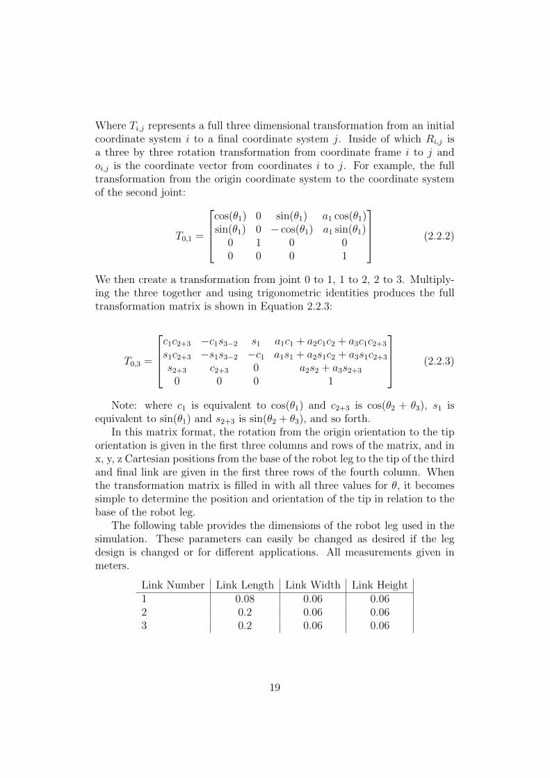
In this matrix format, the rotation from the origin orientation to the tiporientation is given in the first three columns and rows of the matrix, and inx, y, z Cartesian positions from the base of the robot leg to the tip of the thirdand final link are given in the first three rows of the fourth column. Whenthe transformation matrix is filled in with all three values for θ, it becomessimple to determine the position and orientation of the tip in relation to thebase of the robot leg.

The following table provides the dimensions of the robot leg used in thesimulation. These parameters can easily be changed as desired if the legdesign is changed or for different applications. All measurements given inmeters.

Link Number Link Length Link Width Link Height1 0.08 0.06 0.062 0.2 0.06 0.063 0.2 0.06 0.06

19

2.3 SimMechanics Model

Later in this paper we will use Matlab SimMechanics software to verify themathematical model of the robotic leg. This model will be used to ensure thattorques calculated based on desired position, velocity, and acceleration willactually produce the desired positions in simulation. Here, we will introducehow to set up the kinematics of the robotic leg in SimMechanics so that itcan later be used to verify the torque calculations.

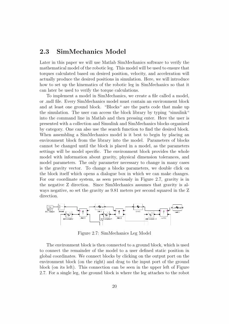
To implement a model in SimMechanics, we create a file called a model,or .mdl file. Every SimMechanics model must contain an environment blockand at least one ground block. “Blocks“ are the parts code that make upthe simulation. The user can access the block library by typing “simulink“into the command line in Matlab and then pressing enter. Here the user ispresented with a collection and Simulink and SimMechanics blocks organizedby category. One can also use the search function to find the desired block.When assembling a SimMechanics model is it best to begin by placing anenvironment block from the library into the model. Parameters of blockscannot be changed until the block is placed in a model, as the parameterssettings will be model specific. The environment block provides the wholemodel with information about gravity, physical dimension tolerances, andmodel parameters. The only parameter necessary to change in many casesis the gravity vector. To change a blocks parameters, we double click onthe block itself which opens a dialogue box in which we can make changes.For our coordinate system, as seen previously in Figure 2.7, gravity is inthe negative Z direction. Since SimMechanics assumes that gravity is al-ways negative, so set the gravity as 9.81 meters per second squared in the Zdirection.

Figure 2.7: SimMechanics Leg Model

The environment block is then connected to a ground block, which is usedto connect the remainder of the model to a user defined static position inglobal coordinates. We connect blocks by clicking on the output port on theenvironment block (on the right) and drag to the input port of the groundblock (on its left). This connection can be seen in the upper left of Figure2.7. For a single leg, the ground block is where the leg attaches to the robot

20

body, and is the origin of the leg coordinate system. In this way we abstractthe robotic leg from the walking robot as a whole. Thus, the location of theground block is set to the origin. Now we can begin to assemble the partsspecific to our own model. From this point we use a joint block to provideour first joint. SimMechanics has a number of different joint block types tochoose from, but here we select the single rotational axis joint. After placingit in the model, we adjust parameters using the dialogue box as shown inFigure 2.8.

Figure 2.8: The dialogue box for defining the parameters of joint 1 in Sim-Mechanics

This block allows us to set the joint’s axis of rotation, which, based onour coordinate system, is in the Z direction. The joint block also requiresa location, this can be determined by its base or follower, we are going touse the base to define the joints coordinates. We connect it to the groundblock by dragging a line from the ground output to the joint input. Now thejoint is located at the origin. The next step is to define the first link of therobotic leg. For this we use a body block. Double clicking on SimMechanicsblocks will open the dialogue box to define its parameters. We fill in eachbody block as shown in Figure 2.9 with physical information, such as mass,the inertia matrix, location of the center of mass, and location of the endpoints where it connects to other blocks. For us we determine the location ofthe base by its base, the origin. As for the CoM and the endpoint, these are

21

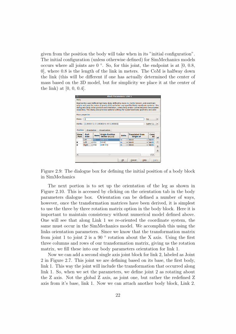
given from the position the body will take when in its ”initial configuration”.The initial configuration (unless otherwise defined) for SimMechanics modelsoccurs where all joints are 0 ◦. So, for this joint, the endpoint is at [0, 0.8,0], where 0.8 is the length of the link in meters. The CoM is halfway downthe link (this will be different if one has actually determined the center ofmass based on the 3D model, but for simplicity we place it at the center ofthe link) at [0, 0, 0.4].

Figure 2.9: The dialogue box for defining the initial position of a body blockin SimMechanics

The next portion is to set up the orientation of the leg as shown inFigure 2.10. This is accessed by clicking on the orientation tab in the bodyparameters dialogue box. Orientation can be defined a number of ways,however, once the transformation matrices have been derived, it is simplestto use the three by three rotation matrix option in the body block. Here it isimportant to maintain consistency without numerical model defined above.One will see that along Link 1 we re-oriented the coordinate system, thesame must occur in the SimMechanics model. We accomplish this using thelinks orientation parameters. Since we know that the transformation matrixfrom joint 1 to joint 2 is a 90 ◦ rotation about the X axis. Using the firstthree columns and rows of our transformation matrix, giving us the rotationmatrix, we fill these into our body parameters orientation for link 1.

Now we can add a second single axis joint block for link 2, labeled as Joint2 in Figure 2.7. This joint we are defining based on its base, the first body,link 1. This way the joint will include the transformation that occurred alonglink 1. So, when we set the parameters, we define joint 2 as rotating aboutthe Z axis. Not the global Z axis, as joint one, but rather the redefined Zaxis from it’s base, link 1. Now we can attach another body block, Link 2.

22

Figure 2.10: Dialogue box for defining the orientation, or change in coordi-nate frames, within a body block in SimMechanics

Once again the inertia matrix, mass, position, and orientation for this linkneed to be defined.

The SimMechanics model also makes use of joint actuators and jointsensors. The actuators allow a user to move a body or joint, and sensorsproduce desired information about the joint. In our model, for each joint,we need to add a joint actuator from the SimMechanics library. As shownin Figure 2.11, to define a joint actuator, one can specify joint torque orjoint movement as an input. The movement option allows the user to inputposition, velocity, and acceleration and the actuator will drive the joint blockmove within those parameters. We however use torque as an input becausethe model is intended to verify the Euler-Lagrange equations that generatethe necessary torques to move the leg. Also, be sure to select the correcttorque units when setting up this block.

Joint sensors are capable of reading position, velocity, acceleration, ex-trapolated torque, or all three using check boxes in the sensor block’s dialoguebox. Since desired position is what we use to drive our torque producing al-gorithm, we seek to verify the model by ensuring that the position read bythe sensors matches what was put into the algorithm, and thus check thoseboxes in the dialogue box.

Note that once this is applied, there will be not one but three ports fromthe sensor block, one for each metric. Parameters for defining a sensor blockare shown in Figure 2.12. In order for the user to view these values, onehas to use what is called a “sink” in the Simulink block library. For initialdevelopment, we used a display or floating scope block, which show real timevalues while the simulation is running. For the final model, we use “to file”

23

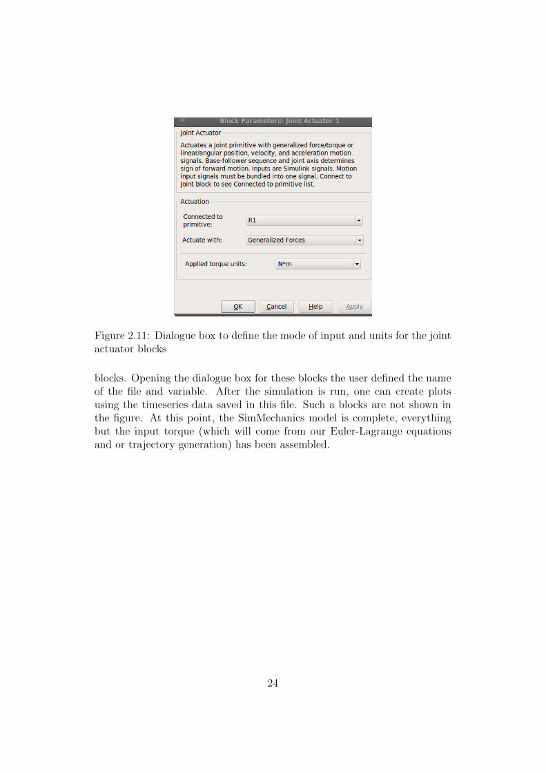
Figure 2.11: Dialogue box to define the mode of input and units for the jointactuator blocks

blocks. Opening the dialogue box for these blocks the user defined the nameof the file and variable. After the simulation is run, one can create plotsusing the timeseries data saved in this file. Such a blocks are not shown inthe figure. At this point, the SimMechanics model is complete, everythingbut the input torque (which will come from our Euler-Lagrange equationsand or trajectory generation) has been assembled.

24

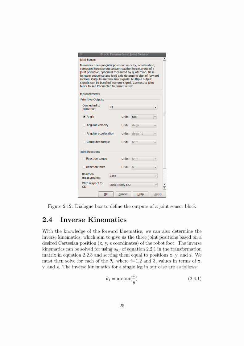
Figure 2.12: Dialogue box to define the outputs of a joint sensor block

2.4 Inverse Kinematics

With the knowledge of the forward kinematics, we can also determine theinverse kinematics, which aim to give us the three joint positions based on adesired Cartesian position (x, y, z coordinates) of the robot foot. The inversekinematics can be solved for using o0,3 of equation 2.2.1 in the transformationmatrix in equation 2.2.3 and setting them equal to positions x, y, and z. Wemust then solve for each of the θi, where i=1,2 and 3, values in terms of x,y, and z. The inverse kinematics for a single leg in our case are as follows:

θ1 = arctan(x

y) (2.4.1)

25

θ2 = − arctan(a3 sin(θ3)

a2 + a3 cos(θ3)+ arcsin(

z√(a2 + a3 cos(θ3))2 + a23 sin(θ3)2

)

(2.4.2)

θ3 = − arccos(( xcos(θ1)

− a1)2 + z2 − a22 − a232a2a3

) (2.4.3)

These calculations can be used for defining a trajectory for the leg in jointspace based on desired leg locations in global Cartesian space.

2.5 The Full Robot Body

Section 2.4 covered the forward and inverse kinematics of a single robot leg,which is similar to calculating the kinematics of any other three degree offreedom manipulator. This project diverges from others with the need tocalculate the forward and inverse kinematics of a full robot body. Instead ofplacing the origin of the coordinates at the first joint, we need to translate theorigin to the center of the robot body. Our robotic body is a simple rectanglewith a number of ports along the perimeter at which legs can be placed, asshown in Figure 2.13. Each port has a unique kinematic transformation from

Figure 2.13: Diagram Robot Body with Ports Numbered

the coordinate system at the base of the leg (joint 1) to a coordinate systemplace at the center of the robot body. For example, the inverse translationfor port 0 is thus:

yrobot = yleg −W

2(2.5.1)

26

xrobot = xleg + 3L

8− pL

4(2.5.2)

zrobot = zleg (2.5.3)

Where W is the width of the robot body, L is its length, and p is the portnumber. As one can see, this is a simple two dimensional shift from port/legcoordinate frame to a coordinate frame at the center of the robot.

2.6 Chapter 2 Summary

In chapter two we began by defining the coordinate systems used to definethe single robot leg. Based on these frames we were able to derive the forwardand inverse kinematics for the single leg. We then discussed the mechanicalfeatures of re-designed robot leg, and how this new design adds improvementsover the previous generation of this robots design. We then introduced use ofthe simulation software SimMechanics, based on Matlab. We walked throughhow to construct a simulation model of the single robot leg using their blocklibrary, and how to set the block parameters using information derived inthe forward kinematics. We then briefly outlined the forward and inversekinematics for translating from coordinate systems in terms of the leg to thosein terms of the whole robot body. With the basic knowledge of the forwardand inverse kinematics, and how to construct a SimMechanics simulationmodel, we can now move forward to define the dynamics and see how theymay be verified using the SimMechanics software.

27

Chapter 3

Robot Leg Dynamics

After understanding the robot in terms of its kinematics, one can begin toinvestigate the dynamics. It is important in modeling a robot motion tocalculate dynamics so that velocity, acceleration, and the forces associatedwith the robot motion are accounted for. In this research, we calculate thenecessary dynamic equations to determine the necessary torques to apply tothe joint in order to produce the desired motion. This produces a dynamicmodel of the leg system which can later be verified.

3.1 Calculating the Jacobian Matrix

Once the kinematic equations have been developed, the next part of creatinga mathematical model of the leg system is to calculate the Jacobian ma-trix. The Jacobian matrix is derived from the transformation matrices andis used for various purposes in robot manipulator control. The Jacobian canbe defined as the relationship between joint velocity and manipulator endvelocity.

ξ = J(q)q (3.1.1)

where ξ is the end of the manipulator velocity and q is a vector of jointvelocities, and J represents the Jacobian matrix.[1] One valuable use of theJacobian is for calculating joint torques necessary in robot leg to maintainconfiguration in response to external forces applied to the foot. This is doneusing using the transpose of the Jacobian matrix, as shown in the equationbelow:

τ = JT (q)F (3.1.2)

where τ is a vector of joint torques, J is the Jacobian of the joint positionvector q, and F a three dimensional vector of force on the robot foot, arranged

28

in the form F = [Fx, Fy, Fz, nx]. This equation will be used in the final robotmodel to incorporate the effect of external forces on the end of leg (the foot).

The Jacobian matrix to be used for these purposes is set out by visualizinga set of equations being multiplied by the set of joint velocities to produceend point velocities:

xyzωxωyωz

=

[Jv1 Jv2 Jv3Jw1 Jw2 Jw3

]∗

θ1θ2θ3

(3.1.3)

where each Jv and Jw are 3x1 column vectors. One can see in the matrix thateach column is associated with a different joint. Each of which is broken intowhat we call the upper and lower Jacobian. Each is also calculated differentlydepending if the joint is prismatic or revolute. All the joints in our leg arerevolute. Therefore, for each Jv:

Jvi = zi−1 × (on − oi−1) (3.1.4)

In which zi the orientation of the z axis after it has been translated fromthe first or origin coordinate frame to the coordinate frame of joint i. Itcan be taken from the last column in the rotation matrix from the originto joint 0, which recall are the first three columns and rows of that sametransformation matrix. oi is the 3x1 coordinate vector from the base of theleg to joint i. It can be taken from the first three values in the last columnof the the transformation matrix from the leg base to joint i. on the threeby one orientation vector for the tip of the robot leg, which is gathered fromthe full transformation matrix from the leg base to the final point of themanipulator. The calculation for Jv2 is provided as an example:

Jv2 = z1 × (o3 − o1) (3.1.5)

Jv2 =

sin(θ1)− cos(θ1

0

×o3−1x

o3−1y

o3−1z

=

− cos(θ1)o3−1z

sin(θ1)o3−1z

sin(θ1)o3−1y + cos(θ1)o3−1x

(3.1.6)

The results of these calculations can be seen in the final Jacobian. As opposedto Jvi, the upper Jacobian which calculates the linear velocities of the joint,Jwi calculates angular velocities, and for each:

Jwi = zi−1 (3.1.7)

29

Which is already known from calculating Jvi. In our case, the fullyassembled Jacobian for the manipulator is:

J =

−a1s1 − a2s1c2 − a3s1c2+3 −c1(a2s2 + a3s2+3) −c1(a3 + s2+3)a1c1 + a2c1c2 + a3c1c2+3 −s1(a2s2 + a3s2+3) −s1(a3 + s2+3)

s2+3 c2+3 a3c2+3

0 s1 s10 −c1 −c11 0 0

(3.1.8)

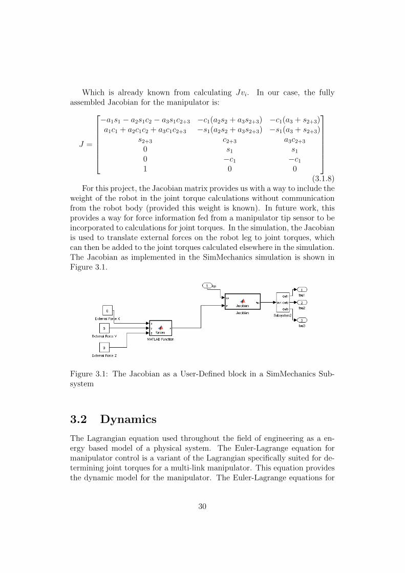
For this project, the Jacobian matrix provides us with a way to include theweight of the robot in the joint torque calculations without communicationfrom the robot body (provided this weight is known). In future work, thisprovides a way for force information fed from a manipulator tip sensor to beincorporated to calculations for joint torques. In the simulation, the Jacobianis used to translate external forces on the robot leg to joint torques, whichcan then be added to the joint torques calculated elsewhere in the simulation.The Jacobian as implemented in the SimMechanics simulation is shown inFigure 3.1.

Figure 3.1: The Jacobian as a User-Defined block in a SimMechanics Sub-system

3.2 Dynamics

The Lagrangian equation used throughout the field of engineering as a en-ergy based model of a physical system. The Euler-Lagrange equation formanipulator control is a variant of the Lagrangian specifically suited for de-termining joint torques for a multi-link manipulator. This equation providesthe dynamic model for the manipulator. The Euler-Lagrange equations for

30

robotic manipulators represent the the overall energy in the robotic leg sys-tem. Using this concept, we can create an equation where one side determinesenergy driven by manipulator configuration (joint position, velocity,and ac-celerations) and the other side to determine the torques required to achievea desired configuration.

3.2.1 Components of the Manipulator Lagrangian

The basic concept for the Lagrangian is set out in equation 3.2.1:

L = K − P (3.2.1)

where the Lagrangian is the difference between kinetic energy terms Kand potential energy P throughout the moving body(s). However, in manip-ulator control, we use the Lagrangian to calculate the various joint torquesnecessary in a manipulator to generate desired joint positions, velocities, andaccelerations. Those equations which provide desired torque are called theEuler-Lagrange equations, and are derived from the calculations collected inthe former sections of this paper. We will be using a common method forcalculating the Euler-Lagrange equations specifically for a robotic manipu-lator made up of rigid-body links [1]. We begin with the kinetic energy for asingle link which is given as:

K =1

2mvT +

1

2ωTIω (3.2.2)

where K is kinetic energy, m is link mass, v is the linear velocity ofthe link at center of mass, ω is rotational velocity of the link, and I is theinertia matrix for the link. One can see the linear and rotational componentsof kinetic energy, where the energy equals one half mass times a velocityvector, plus one half the angular velocity vector multiplied with matrix I,which is our inertia tensor. The inertia calculations are the next part of thepuzzle. This is calculated:

I = RIRT (3.2.3)

In which R is the rotation matrix for that particular link, taken, as men-tioned before, from the first three columns and rows of its transformationmatrix. I however is the inertia matrix, which is calculated based on thephysical properties of the link. If one is working with a specific mechanicaldesign that has been fully specified using 3D modeling software, these param-eters can be taken from the model. In many cases, however, it is sufficient to

31

model the link as a uniform rectangular solid, in which case the inertia canbe calculated as in 3.2.4:

I =

(l2h + l2)m12

0 00 (l2h + l2w)m

120

0 0 (l2 + l2w)m12

(3.2.4)

Where l is the link length, lh is the link height, and lw is link width. Sincewe use the Denavitt-Hartenberg convention, the dimension in which the linkheight is measured parallel to the z axis (parallel to the axis around whichthe previous joint rotates) and the link width is along the x axis, since thelength of the link always runs along the y axis. Now that we have all thenecessary information for each link, we calculate the kinetic energy for ann-link manipulator, which is calculated as in 3.2.5:

K =1

2qT

[n∑i=1

{miJvci(q)TJvci(q) + Jwci(q)

TRi(q)IRi(q)TJwci(q)}

]q (3.2.5)

Many notations will also use D to represent the matrix form of the kineticenergy computed within the brackets above such that:

K =1

2qTDq (3.2.6)

The next variables Jvi and Jwi are the upper and lower halves of a fullJacobian matrix taken from the origin to the center of mass of link i. Theseare not components of the already calculated Jacobian matrix. Instead, onemust calculate each Jacobian matrix for each center of mass i in the sameway as for a full manipulator described in section 3.1.One merely substitutesthe oi variable with oci to represent the center of mass, as shown:

Jvi = zi−1 × (ocn − oi−1) (3.2.7)

Another change is that unlike the full Jacobian matrix to the end of themanipulator, the Jacobian matrix for links 1 and 2 will mean that for somecolumns, i− 1 will be greater than n, in these cases, Jvi or Jwi will be athree by one column of zeros. As an example, take the center of mass on thesecond link.

In the equation for the kinetic energy we also use q and q, which representthree by one vectors of joint positions and velocities, respectively. We take thesummation of the linear and angular velocity components for all the links,depending on their configuration. Next we compute the potential energy

32

for the n-Link manipulator, which is simply a summation of the potentialenergies for each link shown in equation 3.2.8.

P =n∑i=1

migT rci (3.2.8)

In which mi is mass of link i, g is the gravity vector in terms of the basecoordinate frame, and rci provides the coordinates of the center of mass oflink i. from the base to the center of mass of link i.

3.2.2 Methods of Computing the Euler-Lagrange for aManipulator

The next step in this process is to assemble the described matrices into themanipulator Lagrangian by forming the kinetic and potential energy partsand then differentiating to calculate the torques for each joint necessary toproduce the desired manipulator configuration. Two different methods andtwo different software packages were used to compute the Lagrangian.

Let us begin by outlining the computational steps for calculating torqueof each joint using the manipulator Lagrangian. First, the partial derivativeof the Lagrangian with respect to the joint velocity of joint k:

∂L

∂qk=∑j

dkj qj (3.2.9)

Here the j subscript notes columns and rows of the corresponding matri-ces. dk,j represents the jth row of the D matrix for the kth joint. We thentake the full derivative of the same by doing the following:

d

dt

∂L

∂qk=∑j

dkj qj +∑i,j

∂dkj∂qi

qiqj (3.2.10)

We also take the partial derivative of the Lagrangian with respect to thekth joint position:

∂L

∂qk=

1

2

∑i,j

∂dij∂qk

qiqj −∂P

∂qk(3.2.11)

These four components can then be laid out in the following way:∑j

dkj qj +∑i,j

{∂dkj∂qi− 1

2

∂dij∂qk}qiqj +

∂P

∂qk= τk (3.2.12)

33

If we take the first summation to equal D, the two expressions in thebrackets as C, and the last part as G, and adding the Jacobian and externalforces, we have:

τ = Dq + C(q, q)q +G(q) + JTFext (3.2.13)

The result is the the Euler-Lagrange equations in matrix form.The D matrix value comes from taking the second derivative the kinetic

energy of the manipulator, and uses the input of joint acceleration, thusthis factor represents torque based on angular force. The next factor Crepresents what are called the Coriolis and centrifugal or coupling effectsof the manipulator system on joint torques. Note it includes both angularposition and velocity terms. The G matrix includes forces based on theinfluence of gravity. The final factor takes account for external forces on themanipulator tip. Multiplying a vector for external forces by the transverseJacobian results returns the extra torque on each joint due to external forces.

In this project, we used Matlab code to define the various matrices usedin the Euler-Lagrange equations. However, when it came to differentiatingthese matrices, there appeared to be no elegant way to accomplish this inMatlab. It was attempted with Matlab’s symbolic toolbox, however it wasdifficult, if not impossible, to properly define joint accelerations and velocitiesas derivatives of joint position and maintain this definition while Matlabcomputed the time derivative. Eventually, the entire code for calculatingthe Lagrangian was copied to Wolfram Mathematica for the derivations, andthen copied back to Matlab to provide a function that took joint positions,velocities, and accelerations and calculated joint torques that would providethese configurations.

Using Wolfram’s Mathematica software, the Lagrangian was computedby taking a series of derivatives and partial derivatives to the equation. Af-ter setting out the various parts of the Lagrangian, the Mathematica scriptassembled the kinetic energy for the Lagrangian as such:

*The Kinetic energies for each link*

Dk1 = m1 * (Transpose[Jv1].Jv1) + Transpose[Jw1].R1.I1.Transpose[R1].Jw1;

Dk2 = m2 * (Transpose[Jv2].Jv2) + Transpose[Jw2].R2.I2.Transpose[R2].Jw2;

Dk3 = m3 * (Transpose[Jv3].Jv3) + Transpose[Jw3].R3.I3.Transpose[R3].Jw3;

Dtot = Dk1 + Dk2 + Dk3;

This D matrix was multiplied by a vector of joint velocities, and thePotential Energy for each leg was added producing:

L = FullSimplify[(1/2) * Transpose[qdot].Dtot.qdot - (P1 + P2 + P3)]; *7.53*

34

Where the “full simplify” function is used to simplify the result. Thenfor each joint i, the script takes the partial differential of the Lagrangian Lwith respect to velocity qi. This is equivalent to equation 3.2.9 above:

*Partial differentials of Lagrangian with respect to qdot*

Lqdoti = D[L, Dt[qi[t], t]]; *7.55*

then the time derivative of the result, equivalent to equation 3.2.10.

*Derivatives(d/dt*dL/dqdot)*

Lqddoti = Dt[Lqdoti, t]; *7.56*

Then the partial derivative of L with respect to qi just as in equation3.2.11

*Partial Derivatives of Lagrangian with respect to q*

Lqi = D[L, qi[t]];

and finally the torque τi by taking the difference between time derivativeand the partial with respect to qi.

*Calculate Torques t=d/dt* L/dqdot - L/q* *7.42, 7.62*

taui = Chop[FullSimplify[Lqddoti - Lqi]]

The symbolic computations for deriving the dynamic model has been donein Mathematica and MATLAB is used for the numerical implementation.Appendix A presents the Mathematica notebook and Appendix B shows theMatlab script.

The Euler-Lagrange equations were later calculated in Matlab when itwas realized that there existed a method which only used partial derivativeswith respect to qi and not time. With this method, rather than takingtime derivatives it uses the matrix form set out by Spong [1]. To this end,we created the files NewLagrangian.m and Christoffel.m. NewLagrangian.mtakes all the parts from the previous section and uses them to create the D,C, and G matrices. The D matrix is simply:

%Compute portions of D matrix

Dtran1=(m1/2)*Jcv1’*Jcv1;

Dtran2=(m2/2)*Jcv2’*Jcv2;

Dtran3=(m3/2)*Jcv3’*Jcv3;

Drot1=Jcw1’*R1*I1*R1’*Jcw1;

Drot2=Jcw2’*R2*I2*R2’*Jcw2;

Drot3=Jcw3’*R3*I3*R3’*Jcw3;

D=Dtran1+Dtran2+Dtran3+Drot1+Drot2+Drot3;

35

where each component of the D matrix, Dk,j, are used in the torquecalculation as shown in 3.2.12. The components of the C matrix are generatedusing the function Christoffel.m which is:

function c=Christoffel(D,q,i,j,k)

c=(1/2)*(diff(D(k,j),q(i))+diff(D(k,i),q(j))-diff(D(i,j),q(k)));

Which takes the D matrix and a vector of three q values, and calculatesthe Christoffel symbols for any i, j, or k. The symbols are then used asfollowing:

%Compute Christoffel Symbols:

c11=Christoffel(D,q,1,1,k);

c12=Christoffel(D,q,1,2,k); %=c21

c22=Christoffel(D,q,2,2,k);

c13=Christoffel(D,q,1,3,k); %=c31

c23=Christoffel(D,q,3,2,k); %=c32

c33=Christoffel(D,q,3,3,k);

Here the Christoffel symbols are calculated for a single k value, since inthis code k denotes the joint number that the function is calculating torquefor. The code is modeled after the equations shown in in 3.2.14 and 3.2.15.

cijk =1

2{∂dkj∂qi

+∂dki∂qj− ∂dij∂qk} (3.2.14)

Where the (k, j)th element of the C matrix is:

ckj =n∑i=1

cijk(q)qi (3.2.15)

The G matrix components, which is actually a column vector of the po-tential energies for each link, is computed:

g=diff(P,q(k));

Which is computed for each joint k. As is the torque, as shown below:

tau=D(k,1)*q1ddot+D(k,2)*q2ddot+D(k,3)*q3ddot ...

+ c11*q1dot^2+2*c12*q1dot*q2dot+c22*q2dot^2 ...

+ 2*c13*q1dot*q3dot+2*c23*q2dot*q3dot+c33*q3dot^2+g;

This result of this calculation was also used in the Matlab script placedin the SimMechanics simulation in the same way that the torque calculationfrom Mathematica was, however, once again, it was to no avail.

36

3.3 Using User Defined Blocks

In SimMechanics, one can create mathematical functions using series of mathfunction blocks, however, with lengthy calculations it seemed best to createuser defined blocks. This is the case with the Euler-Lagrange equations. InMatlab, each can be set out as a Matlab function, in which joint position,velocity, and acceleration are input and the torque the output. To place sucha function, one places a “user defined block” from the Simulink functionlibrary into the model. After double clicking the block, the user is presentedwith a box that looks identical to that of the standard Matlab function. Aftercoding out the Lagrangian from either method described above, click okay.The result is then a user defined block with a number of inputs equivalentto the number of inputs defined by the function, and a single output.

3.4 Chapter 3 Summary

In this chapter we discussed how to assemble the matrix components for theEuler-Lagrange equations. These included: Jacobians (revolute and linear)for each links center of mass, rotation matrices, the initial matrices, and po-tential energy. These parts were then assembled into a kinetic and potentialenergy matrix. This chapter then outlined two different methods for takingthe necessary derivatives to calculate torque. Finally, we described how toincorporate the equation for torque into the SimMechanics model.

37

Chapter 4

Simulating the Leg

The overall simulation for the robot leg dynamics is broken down into threebasic subsystems: trajectory generation, the dynamic model, and the simula-tion of the robot leg; shown in Figure 4.1. The trajectory generation function

Figure 4.1: High Level Diagram of the overall SimMechanics Simulation forthe Robotic Leg

for this model is for a single step, but using a control loop, the model couldeasily be altered to make it adaptive on each iteration. It is currently con-stant in the sense that it moves through the same set points for each step,as though assuming flat terrain. An adaptive step would mean that the setpoints which define the step’s trajectory could be changed for each step based

38

on what the robot may know about its environment through sensors.Currently it takes constant user inputs for desired step location and step

length, the trajectory generation function generates the necessary joint posi-tions, velocities, and accelerations needed to achieve a smooth motion frompoint to point. This “subsystem” will be described in detail later in thischapter.

The dynamic model portion of the simulation is made up of several user-defined blocks. These blocks behave in the same manner as any other blockin Simulink, but instead of setting various parameters, the blocks inputs andoutputs are determined based on Matlab code placed inside the block. Userdefined blocks are the only option for integrating a mathematical model ashigh level as the dynamics for this project into a Simulink simulation. Themathematical model for calculating joint torques has already been describedthroughout this paper, thus, it is convenient to build SimMechanics modelwhile determining the environment and kinematics.

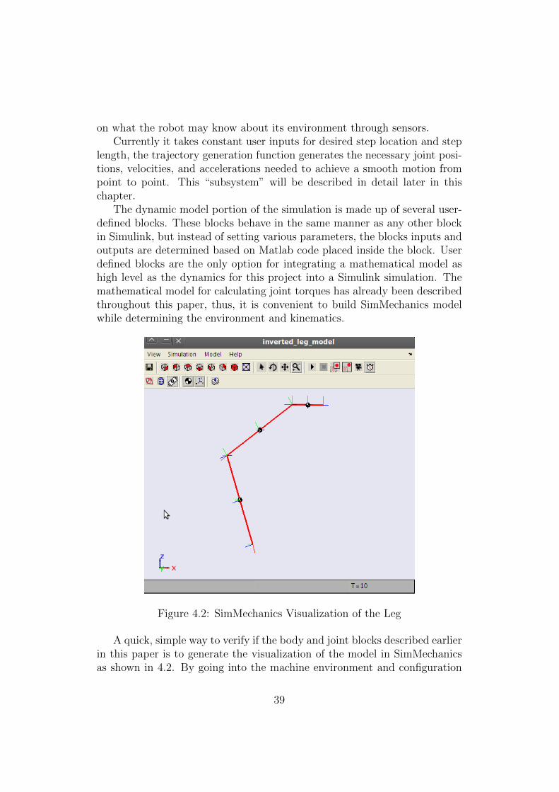
Figure 4.2: SimMechanics Visualization of the Leg

A quick, simple way to verify if the body and joint blocks described earlierin this paper is to generate the visualization of the model in SimMechanicsas shown in 4.2. By going into the machine environment and configuration

39

parameters, one can select an option to run a visualization of the model whileit is running. This will produce a pop-up window of the model moving inreal time. This will help to verify that the coordinate frames for the links.Also, we use it to determine if the movement of the leg over time followsthe trajectory we expect to see. Meaning that we will see the foot liftingup, setting back down, and moving across the ground rather than movingirrationally; for example lifting the leg further up rather than stepping down.

4.1 Leg Trajectory

One challenge in robot control is setting trajectories for robotic manipulators.This effort will be entirely configuration dependent, meaning the design ofa trajectory depends both on the structure of the manipulator (our roboticleg) and the intent of the movement. The movement must not go outside ofthe range of the manipulator, velocities and accelerations must be smoothto avoid sudden jerks or physically impossible jumps, and for a leg the stepmust not upset the balance of the robot.

For the sake of this simulation, a trajectory had to be chosen to makea single robotic step. The trajectory generated for this simulation is onethat would maintain stable walking on a flat, level surface. The simulationis left open to be able to accept inputs from another source and thus be ableto adjust changing step lengths and heights, so as to be able to step on oraround obstacles. This other source would need to evaluate the surface thatthe robot needed to navigate, and then provide to the simulation a place onwhich to set the foot which was within the workspace of the leg and allowedthe leg to provide support for the body. The point chosen for the simulationhave been verified to fulfill these criteria.

4.1.1 Workspace

To design a trajectory for the robotic leg, first we need to ensure that desiredlocations for the foot or tip of the robotic leg, as well as a path between theselocations, are within the workspace of the manipulator. The workspace isthe area that the foot can reach given its geometry, joint limits, and degreesof freedom. We can visualize the workspace by using the forward kinematicsfor the leg and plotting in space the location of the leg tip at every possiblejoint configuration. Such a set of points is graphed using Matlab to showpotential workspace for the tip of our robot leg (the foot) in four views shownin Figure 4.3.

Here the “top” view is parallel to the robot body, or perpendicular to the

40

Figure 4.3: Workspace for Robot Leg

plane on which the leg is mounted. The front view is also perpendicular tothe frame on which the leg is mounted, and parallel to the first link when itis in the zero position. The fourth view, “right” is position in parallel withthe plane on which the robot leg is mounted.

4.1.2 Set Points

The trajectory for this leg was generated by determining x, y, and z positionswithin Cartesian space in the same coordinate frame as the base of the legas set points for the leg to reach during the step. An example is shown inFigure 4.4.

For a step, there are three points of particular interest. First, the anteriorextreme position, or the farthest position in front of the robot. This is wherethe foot should be just before placing weight on the leg. Next is the posteriorextreme position, the farthest position behind the robot, and where the footshould be when the robot takes weight off the leg. Third we will call themax height position, which represents the half-way point of when the robotis swinging the leg forward for the next step. These three points define three

41

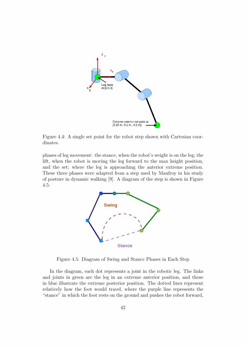
Figure 4.4: A single set point for the robot step shown with Cartesian coor-dinates.

phases of leg movement: the stance, when the robot’s weight is on the leg; thelift, when the robot is moving the leg forward to the max height position,and the set; where the leg is approaching the anterior extreme position.These three phases were adapted from a step used by Maufroy in his studyof posture in dynamic walking [9]. A diagram of the step is shown in Figure4.5:

Figure 4.5: Diagram of Swing and Stance Phases in Each Step

In the diagram, each dot represents a joint in the robotic leg. The linksand joints in green are the leg in an extreme anterior position, and thosein blue illustrate the extreme posterior position. The dotted lines representrelatively how the foot would travel, where the purple line represents the“stance” in which the foot rests on the ground and pushes the robot forward,

42

and the “swing” phase in red in which the foot lifts up from the extremeposterior position and sets down again in the extreme anterior position.

4.1.3 Generating Smooth Trajectories

Now that these points are defined, we need to outline the leg’s positionbetween these points. Note also that the three points we outline all representa change in direction for the leg. Since inertia plays a significant role in robotdynamics, we wish to limit sudden changes in robot velocity. For this reason,our simulation then solves a quintic trajectory equation to get a set of jointpositions, velocities, and accelerations for a number of time steps in betweenthe points. It is called a quintic trajectory because in order to allow all threeorders of motion (position, velocity, and acceleration) to begin and end atzero, one must create a path for position that is a fifth order polynomial.

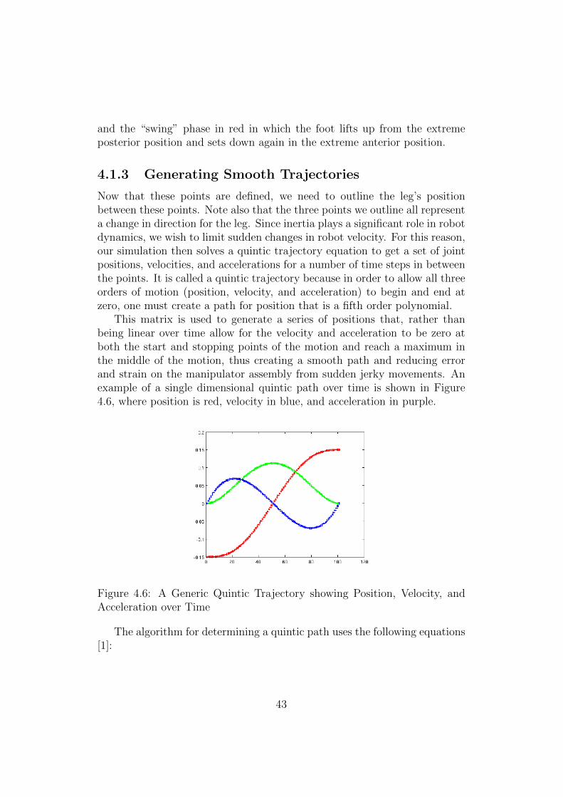
This matrix is used to generate a series of positions that, rather thanbeing linear over time allow for the velocity and acceleration to be zero atboth the start and stopping points of the motion and reach a maximum inthe middle of the motion, thus creating a smooth path and reducing errorand strain on the manipulator assembly from sudden jerky movements. Anexample of a single dimensional quintic path over time is shown in Figure4.6, where position is red, velocity in blue, and acceleration in purple.

Figure 4.6: A Generic Quintic Trajectory showing Position, Velocity, andAcceleration over Time

The algorithm for determining a quintic path uses the following equations[1]:

43

1 t0 t20 t30 t40 t500 1 2t0 3t20 4t30 5t400 0 2 6t0 12t20 20t301 tf t2f t3f t4f t5f0 1 2tf 3t2f 4t3f 5t4f0 0 2 6tf 12t2f 20t3f

×A0

A1

A2

A3

A4

A5

=

p0v0a0pfvfqf

(4.1.1)

where t0 and tf are the initial and final times over which the quintictrajectory will run, p0 and pf are the initial and final positions, v0 and vf theinitial and final velocities, and a0 and af the initial and final accelerations.The A column vector is made up of the quintic coefficients needed to achievea solution of desired initial and final positions, velocities and accelerationsover the given time span. An algorithm that solves for the A coefficientsbased on the quintic matrix and desired initial and final positions, velocities,and accelerations was coded in Matlab for use in the simulation. Throughoutthe simulation, initial and final positions and time come from user definedconstants, and the initial and final velocities and accelerations are set asconstants. The solution for our position trajectory is shown in equation

p(t) = a0 + a1t+ a2t2 + a3t

3 + a4t4 + a5t

5 (4.1.2)

Where ai are the values of the column vector A. The equations for veloc-ity and acceleration are simply derivatives of this equation. The quintic pathcan be used in one of two ways. In the first method generates the desiredset points and finds the inverse kinematics of each. The quintic path is thenused to determine the range of joint positions as the robot leg travels fromone configuration to the next. This generates a smooth curve for position,velocity, and acceleration of each joint. This continuous curve is convenientto use in modeling software such as Simulink because a continuous signalcan easily be manipulated. The drawback of this approach however is thatthe leg will move in a manner that is most convenient for the joints, andthe manipulator configuration in between the set points is left uncontrolled.Using the second method differs only in one determines primary set points,and then a full curve of points in each global x, y, and z dimensions betweenthe primary ones. This differs in the sense that the curves of points aregenerated before the inverse kinematics are calculated. Using this method,one can deterministically decide the location of every point the manipulatortip reaches throughout its motion. We use the quintic trajectory to generatethe curve of points between the primary set points. After these points aredetermined, the inverse kinematics are calculated for each. The major draw-back here is that the final trajectory of joint position will not be a smooth

44

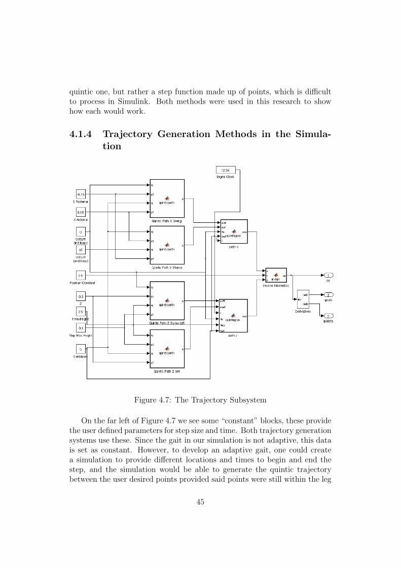
quintic one, but rather a step function made up of points, which is difficultto process in Simulink. Both methods were used in this research to showhow each would work.

4.1.4 Trajectory Generation Methods in the Simula-tion

Figure 4.7: The Trajectory Subsystem

On the far left of Figure 4.7 we see some “constant” blocks, these providethe user defined parameters for step size and time. Both trajectory generationsystems use these. Since the gait in our simulation is not adaptive, this datais set as constant. However, to develop an adaptive gait, one could createa simulation to provide different locations and times to begin and end thestep, and the simulation would be able to generate the quintic trajectorybetween the user desired points provided said points were still within the leg

45

workspace. The next step for this method is to generate the set of pointsbetween these constant primary set points. This is done by four quintic pathblocks, one for each phase and stage over which the step moves. The pathin the global x direction (along the body of the robot) is broken up into twostages, the swing and stance.

The swing is for stepping forward, and the stance for when the robotsweight is supported by the leg. The z direction is also broken up into twostages, these are both for the robot’s step, one for lifting the leg and anotherfor setting it down. During the stance phase z remains constant. Movementin the y direction for the entire step is constant. When any of the variablesremain constant, they do not need to be put through the quintic trajectoryblock, but rather are routed directly to the inverse kinematics for each stepas shown in Figure 4.7.

These are user defined blocks coded to solve for the quintic trajectorysolution; the A matrix of polynomials which define the quintic path. TheA matrix is then passed on to another user defined block which generatesthe quintic position. This block is unique in that it also contains an “if-then” condition that decides which A matrix to use to generate the positiondepending on what stage in the the step the simulation is in.

Finally, the positions go through the inverse kinematics to generate thejoint positions necessary to reach the Cartesian set points given in terms ofthe coordinate frame on the base of the leg. The set of joint positions andpass on through two more blocks to generate its two derivatives, velocity,and acceleration. These three, for each joint, can then be passed on to therest of the simulation. The process of taking the derivatives for this functionis discussed later in this section. The resulting trajectory for a single step injoint space is shown in the graphs with position in red, velocity in blue, andacceleration in green in Figure 4.8.

The second method works very differently in the simulation, starting withthe given constant primary set points they are each passed directly onto theinverse kinematics. Recall that for each stage of the step, the set points willeither serve as the start or end point. For this reason, the three set points,converted into joint space, are fed into Simulink switch blocks. This can beseen in Figure 4.9.

A user defined function based on system time in the trajectory subsystemcontrols the switch, telling it to select whichever set of joint positions isappropriate depending on the stage in the simulation. The selected jointpositions are sent to three quintic trajectory blocks, which solve for the Amatrix for each joint. The subsystem then returns the joint position, velocityand acceleration as determined by the A matrix by the method outlinedearlier in this section. In this manner, the position, velocity, and acceleration

46

Figure 4.8: Joint Position, Velocity, and Acceleration over Time

are all smooth polynomial functions. As seen in the graphs in Figure 4.10.

4.1.5 Stability Polygon

This set of chosen joint positions used for the simulation were tested using aMatlab script which generates a stick model, as shown in Figure 4.11: Thisstick model was generated with a Matlab script that draws four legs attachedat the four corner ports. This script can also be used for any number of legslocated at any of the specified ports on the robot body. Note the triangleon the “floor“ (a flat plane drawn between the three ”feet” on the ground)which represents the stability polygon. This merely draws a shape on thefloor between the remaining feet that are not actively taking a step. Thereis also a blue circle in this diagram.

This circle represents the whole robot’s center of mass projected on thefloor. This stick model is a convenient way to determine if a joint configura-tion is possible and what it will look like. More importantly, it determinesif a set of joint positions for each leg combined does not throw the robotscenter of mass outside the stability polygon, thus causing the robot to fallover.

47

Figure 4.9: The Trajectory Subsystem

4.1.6 Checking for Singularities and Manipulability

Another potential issue to check for is areas in the trajectory where thelegs motion may be limited by its configuration. This can be caused by asingularity or particularly small manipulability in the configuration that theleg was desired to be in at the time the error occurred. A simple script waswritten using the Jacobian described in Section 3.1 to determine the rankof the Jacobian and the manipulability for each configuration in the desiredtrajectory. This is done to check if there is a singularity at the time whenthe data shows an asymptote or when the solver returns an error.

Jacobian matrix will help to identify singularities and calculate manip-ulability of the leg in certain configurations. Singularities occur when therank of the Jacobian matrix is less than six, meaning when it has less thansix linearly independent columns. Physically, this means that the leg is notable to reach certain velocities in the configuration defined as a singularity.Singularities can be found by calculating:

rankJ(q) < 6 (4.1.3)

for every joint configuration. In the same way, the manipulability (ability forthe leg to move within global space) for each configuration is calculated:

µ =√det(JT (q)J(q)) (4.1.4)

A singularity is indicated by a rank of less than three, where the leg maynot be able to attain certain velocities. Low manipulability would indicatethat the movement of the leg in that configuration is limited. The data canbe seen graphically in Figures 4.12 and 4.13.

48

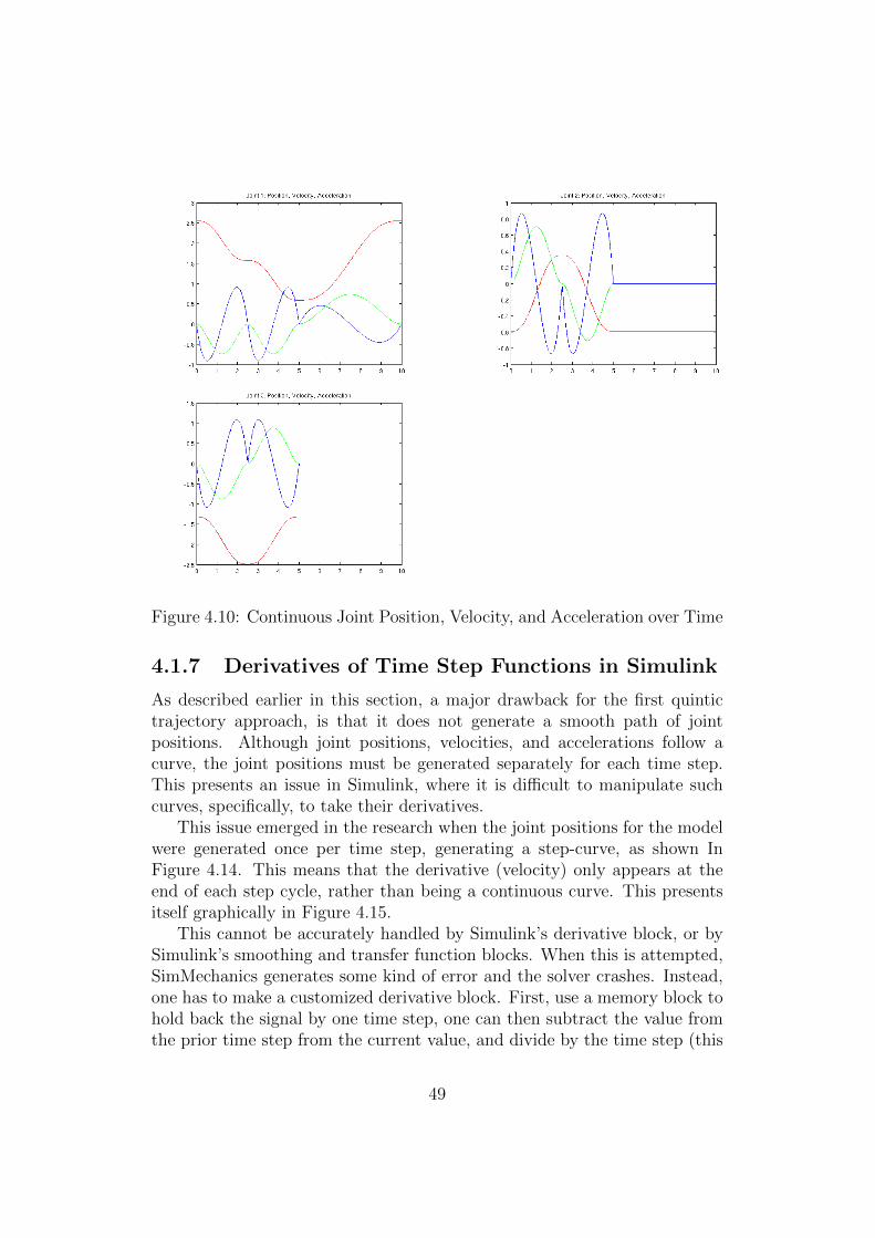
Figure 4.10: Continuous Joint Position, Velocity, and Acceleration over Time

4.1.7 Derivatives of Time Step Functions in Simulink

As described earlier in this section, a major drawback for the first quintictrajectory approach, is that it does not generate a smooth path of jointpositions. Although joint positions, velocities, and accelerations follow acurve, the joint positions must be generated separately for each time step.This presents an issue in Simulink, where it is difficult to manipulate suchcurves, specifically, to take their derivatives.

This issue emerged in the research when the joint positions for the modelwere generated once per time step, generating a step-curve, as shown InFigure 4.14. This means that the derivative (velocity) only appears at theend of each step cycle, rather than being a continuous curve. This presentsitself graphically in Figure 4.15.

This cannot be accurately handled by Simulink’s derivative block, or bySimulink’s smoothing and transfer function blocks. When this is attempted,SimMechanics generates some kind of error and the solver crashes. Instead,one has to make a customized derivative block. First, use a memory block tohold back the signal by one time step, one can then subtract the value fromthe prior time step from the current value, and divide by the time step (this

49

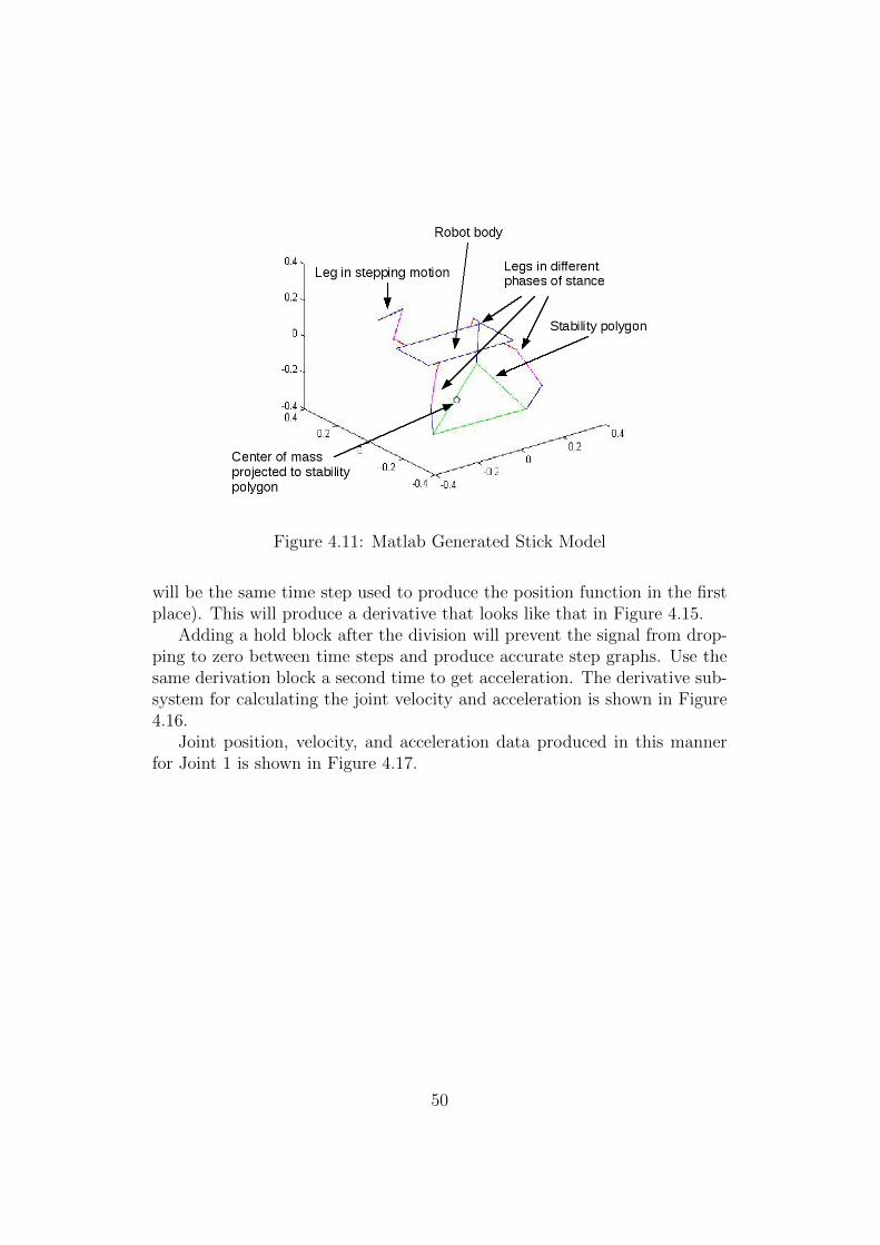
Figure 4.11: Matlab Generated Stick Model

will be the same time step used to produce the position function in the firstplace). This will produce a derivative that looks like that in Figure 4.15.

Adding a hold block after the division will prevent the signal from drop-ping to zero between time steps and produce accurate step graphs. Use thesame derivation block a second time to get acceleration. The derivative sub-system for calculating the joint velocity and acceleration is shown in Figure4.16.

Joint position, velocity, and acceleration data produced in this mannerfor Joint 1 is shown in Figure 4.17.

50

Figure 4.12: Rank of Jacobian overTime based on Configuration

Figure 4.13: Manipulability (µ) overTime based on Configuration

Figure 4.14: Section of joint positionover time graph, zoomed in to showstep detail

Figure 4.15: Section of joint velocityover time graph, zoomed in to showspikes

Figure 4.16: SimMechanics subsystem used to take derivative of non-continuous trajectory

51

Figure 4.17: Joint 1 Position, Velocity, and Acceleration Data, with Deriva-tives Calculated using Described Subsystem

52

4.2 User Defined Blocks

The math for the dynamic model was implemented in the simulation asthree user-defined blocks, one to calculate torque for each joint. Each blockrequires inputs of joint position, velocity, and acceleration for all three joints.The blocks contain the dynamic equations produced by the process outlinedin the subsection on dynamics earlier in the paper. They are used to senddesired torque to the joint actuator block in the SimMechanics model asdescribed in Section 2.3 and shown in Figure 2.8.

The Jacobian is also incorporated into our SimMechanics model using auser-defined block. The user can input a force vector using global X, Y, andZ coordinates to be applied on the manipulator end. The Jacobian blockcan then calculate a set of three torques that would be needed to counteractthat force. These torques are then added to the torques calculated by thedynamic model before being applied to the joint actuators.

For both user defined blocks, there are variables within the Matlab scriptsthat can be changed. As mentioned before, this model was designed such thatthe user could change the parameters to suit a similar robot with slightlydifferent physical features. For example, one can change the dimensions andmass of the links without having to derive the full dynamic model all overagain. This must be done by changing the values in two places. First, thatparameter must be changed in the SimMechanics block which defines thatlink, and recalculate the moment of inertia in the body block to reflect thechange in physical properties. Then we need to change the value in thedynamic model to match. This must be done by opening the user definedblocks, and changing that variable in the beginning of the Matlab code.These variables should be sufficiently labeled and commented to enable theuser to find the desired variable to change and change it. The value of theuser defined blocks is in part that anyone who understands Matlab can easilyunderstand the blocks and alter them as desired.

4.3 Verifying the Simulink Model

The full Simulink model is comprised of the following sub-systems: trajec-tory generation, Euler-Lagrange dynamic equations, the Jacobian, and theSimMechanics physical model. This can be seen in Figure 4.18.

Here we can see all the subsystems together in the same model. First thetrajectory generation on the far left, which sends out all three joint positions,velocities, and accelerations to each of the three user-defined Lagrangianblocks. The three Lagrangian blocks together make up the mathematical

53

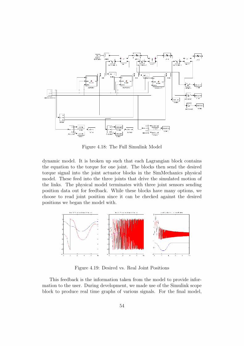
Figure 4.18: The Full Simulink Model

dynamic model. It is broken up such that each Lagrangian block containsthe equation to the torque for one joint. The blocks then send the desiredtorque signal into the joint actuator blocks in the SimMechanics physicalmodel. These feed into the three joints that drive the simulated motion ofthe links. The physical model terminates with three joint sensors sendingposition data out for feedback. While these blocks have many options, wechoose to read joint position since it can be checked against the desiredpositions we began the model with.

Figure 4.19: Desired vs. Real Joint Positions

This feedback is the information taken from the model to provide infor-mation to the user. During development, we made use of the Simulink scopeblock to produce real time graphs of various signals. For the final model,

54

Figure 4.20: Desired vs. Real Joint Positions using Continuous Trajectory

and to see trends in the graph over the full run-time, it is best to save datato file. This sends the data to a timeseries that can be displayed later usingMatlab plot commands.

The simulation seeks to verify the mathematical model by testing if thetorques sent into the joint actuators actually move the joints into the desiredconfiguration. The goal of the Euler-Lagrange equations is to calculate thetorques necessary to achieve the desired configuration. If the math for thetorque generation is correct, the torques generated should move the leg alongthe desired trajectory over time. If the dynamic model is correct, and thesimulation parameters are set up correctly the joint position from the jointsensors and desired joint positions should match. In Figure 4.19 and 4.20,the two can be seen with desired and blue and actual position in red for eachjoint, using both the non-continuous and continuous trajectories.

As the reader can see, these two graphs are entirely different. The desiredposition in blue is a continuous curve which one would expect, however,the actual results in red are not remotely close to the desired trajectory, infact, they almost appear to be noise. This is not actually noise, but rathernumerical error. The graphs demonstrate that instead of smoothly movingfrom one configuration to the next, the joints on the leg rotate around andaround erratically. Troubleshooting performed and possible explainations forthis error will be discussed in the following section.

55

Chapter 5

Conclusions and Future Work

5.1 Results

5.1.1 Simulation Result Analysis

In Section 4.3 in figures 4.19 and 4.20, desired position is compared to modelposition. The desired position is correct, however the actual position looksmore like noise. This is the case when specified torque is incorrect. Thecombined effects of the torque, gravity, and inertia leave us with a set ofjoints that move wildly. We did not limit the range of movement for themodel since the expected positions were well within this range, as verified bythe stick model. However, when torque is incorrect this allows the model toswing the links in full rotations about their joints, leading to the spikes seenin the resulting position graph.

5.2 Inverting the Model

As mentioned earlier in this paper, blocks in SimMechanics can be configureda number of different ways. Using the same series of body and joint blocks inour system model, one can invert its purpose. Rather than generating jointpositions as a result of torque inputs, we can generate torques as a result ofdesired position, velocity, and acceleration.

Our first simulation models how the robotic leg is actually constructed.It utilizes actuator blocks that act as simulated motors that move the con-nected joints in response to a specified torque input. The model then readsposition feedback from sensors attached to these same joints. However, inSimMechanics, one can also actuate joints using desired position, velocity,and acceleration. The joint sensor block can also be configured to provide

56

Figure 5.1: Full Model Inverted

the user with the computed torque values to achieve the position that theattached joint is in. This model, shown in Figure 5.1 a model does exactlythe inverse of our first model. We set up the inverted model to show thenecessary torques to achieve the desired position, and compared them to thetorques produced by the Euler-Lagrange calculations to verify. With thisinverted model, we can use the same trajectory blocks used in the forwardmodel to ensure that the two are working with identical driving data. Theresults are shown in Figures 5.2 and 5.3 using both the trajectory generationsubsystems described earlier in this paper.

Figure 5.2: Calculated Torque (green) vs. Simulation Torque (blue)

Looking at the two, they have similar curvature however the graphicalpeaks differ in amplitude and there are some asymptotes in the calculatedtorque that do not appear in the calculated torque. The differences in inputtorque vs the torque that the model suggests should be used is enough tooffset the results. So much so that using our input torque, the desired position

57

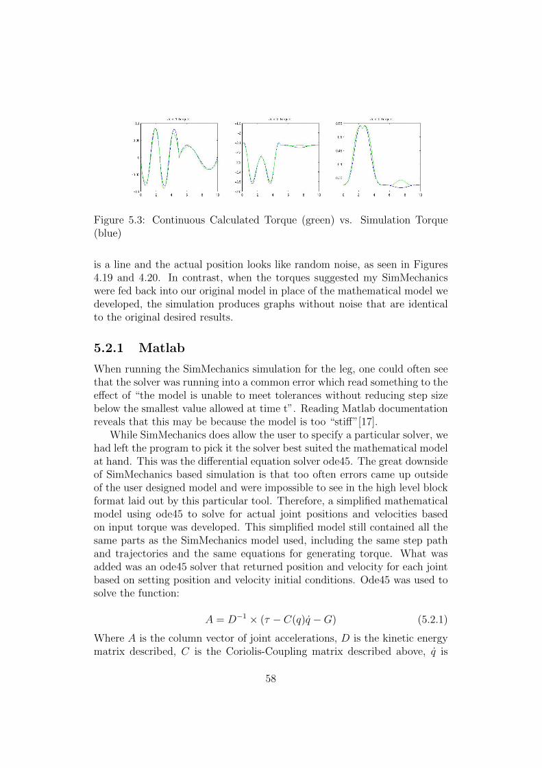
Figure 5.3: Continuous Calculated Torque (green) vs. Simulation Torque(blue)

is a line and the actual position looks like random noise, as seen in Figures4.19 and 4.20. In contrast, when the torques suggested my SimMechanicswere fed back into our original model in place of the mathematical model wedeveloped, the simulation produces graphs without noise that are identicalto the original desired results.

5.2.1 Matlab

When running the SimMechanics simulation for the leg, one could often seethat the solver was running into a common error which read something to theeffect of “the model is unable to meet tolerances without reducing step sizebelow the smallest value allowed at time t”. Reading Matlab documentationreveals that this may be because the model is too “stiff”[17].

While SimMechanics does allow the user to specify a particular solver, wehad left the program to pick it the solver best suited the mathematical modelat hand. This was the differential equation solver ode45. The great downsideof SimMechanics based simulation is that too often errors came up outsideof the user designed model and were impossible to see in the high level blockformat laid out by this particular tool. Therefore, a simplified mathematicalmodel using ode45 to solve for actual joint positions and velocities basedon input torque was developed. This simplified model still contained all thesame parts as the SimMechanics model used, including the same step pathand trajectories and the same equations for generating torque. What wasadded was an ode45 solver that returned position and velocity for each jointbased on setting position and velocity initial conditions. Ode45 was used tosolve the function:

A = D−1 × (τ − C(q)q −G) (5.2.1)

Where A is the column vector of joint accelerations, D is the kinetic energymatrix described, C is the Coriolis-Coupling matrix described above, q is

58

a column vector of joint velocities and G is a column vector of potentialenergy on each link. Each matrix is configuration dependent. The solverwas run in a loop in which initial position and velocity was set as the desiredvalues based on the desired trajectory, and initial torque set as desired torquegenerated by the Euler Lagrange equations. The full set of Matlab scriptsand functions used for this work is contained in Appendix C.

Figure 5.4: Desired Position, Velocity, and Acceleration

Running this mathematical model proved to have very different resultsfrom the SimMechanics simulation. Here the model returned a curve thatwas at least recognizable as the desired position and velocity. The exceptionof course are the “spikes” of simulation noise that occurred. Figure 5.4 showsthe original desired position, velocity, and acceleration which has been keptconsistent since its development for the SimMechanics model. Next, Figure5.5 shows the results returned by Matlab’s ode45 solver.

The spikes seen in the graphs represent some inaccuracies and systemnoise in this area. Note that the time scaling on these graphs goes to 5000,this is because ode45 solved for 50 time steps each time it was run, and theloop was run 100 times. If one looks back to the manipulability graph overtime (Figure 4.12), one can see that the spikes occur mostly in the first area

59

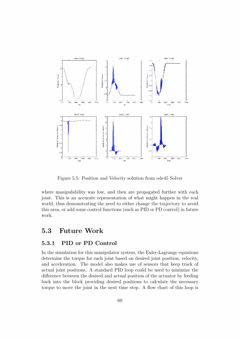
Figure 5.5: Position and Velocity solution from ode45 Solver

where manipulability was low, and then are propagated further with eachjoint. This is an accurate representation of what might happen in the realworld, thus demonstrating the need to either change the trajectory to avoidthis area, or add some control functions (such as PID or PD control) in futurework.

5.3 Future Work

5.3.1 PID or PD Control

In the simulation for this manipulator system, the Euler-Lagrange equationsdetermine the torque for each joint based on desired joint position, velocity,and acceleration. The model also makes use of sensors that keep track ofactual joint positions. A standard PID loop could be used to minimize thedifference between the desired and actual position of the actuator by feedingback into the block providing desired positions to calculate the necessarytorque to move the joint in the next time step. A flow chart of this loop is

60

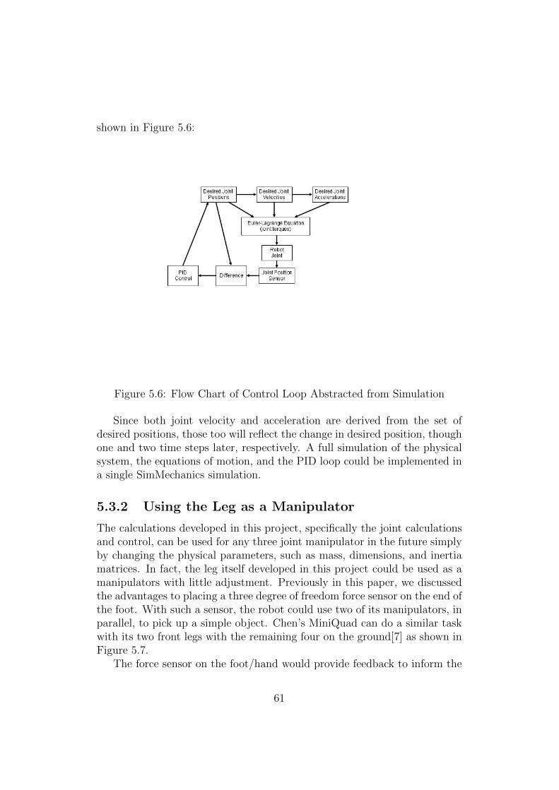
shown in Figure 5.6:

Figure 5.6: Flow Chart of Control Loop Abstracted from Simulation

Since both joint velocity and acceleration are derived from the set ofdesired positions, those too will reflect the change in desired position, thoughone and two time steps later, respectively. A full simulation of the physicalsystem, the equations of motion, and the PID loop could be implemented ina single SimMechanics simulation.

5.3.2 Using the Leg as a Manipulator

The calculations developed in this project, specifically the joint calculationsand control, can be used for any three joint manipulator in the future simplyby changing the physical parameters, such as mass, dimensions, and inertiamatrices. In fact, the leg itself developed in this project could be used as amanipulators with little adjustment. Previously in this paper, we discussedthe advantages to placing a three degree of freedom force sensor on the end ofthe foot. With such a sensor, the robot could use two of its manipulators, inparallel, to pick up a simple object. Chen’s MiniQuad can do a similar taskwith its two front legs with the remaining four on the ground[7] as shown inFigure 5.7.

The force sensor on the foot/hand would provide feedback to inform the

61

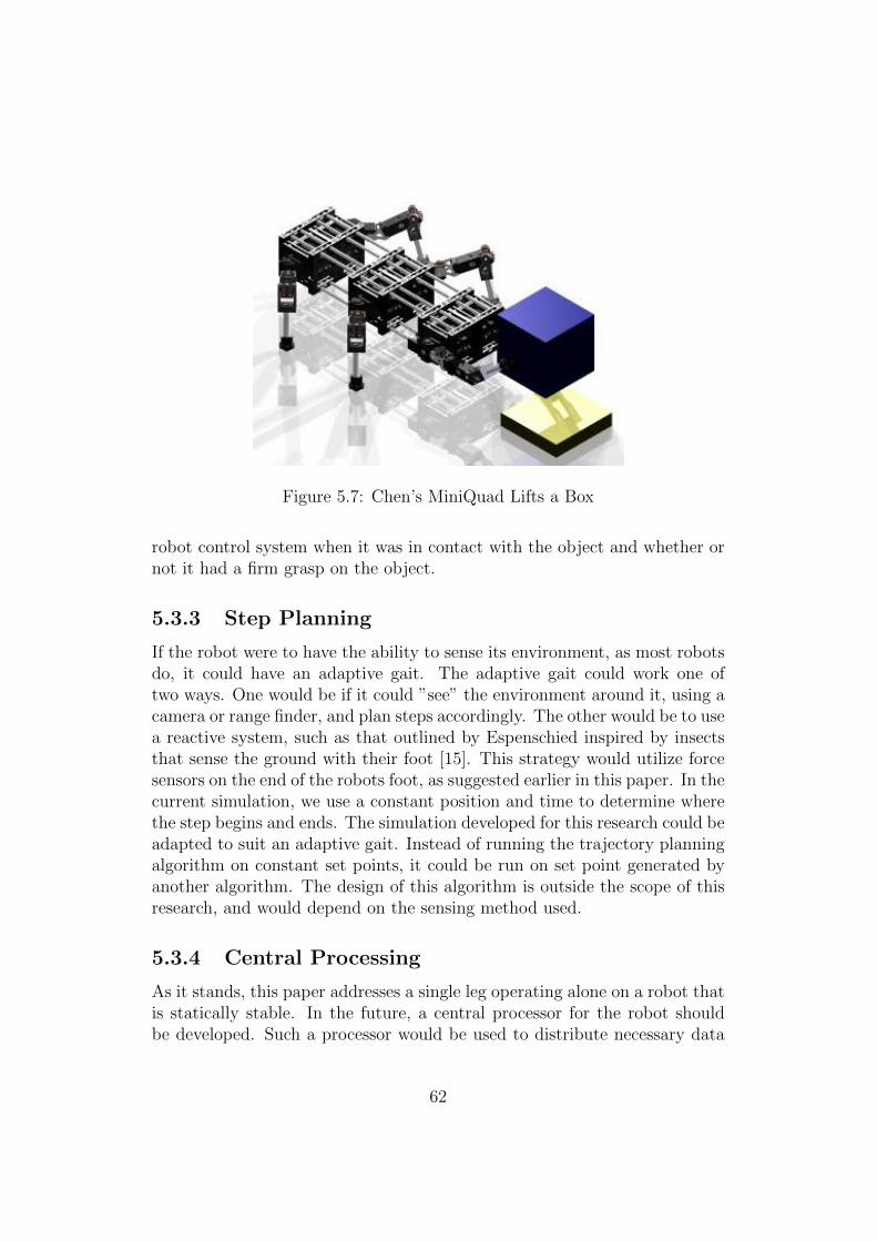
Figure 5.7: Chen’s MiniQuad Lifts a Box

robot control system when it was in contact with the object and whether ornot it had a firm grasp on the object.

5.3.3 Step Planning

If the robot were to have the ability to sense its environment, as most robotsdo, it could have an adaptive gait. The adaptive gait could work one oftwo ways. One would be if it could ”see” the environment around it, using acamera or range finder, and plan steps accordingly. The other would be to usea reactive system, such as that outlined by Espenschied inspired by insectsthat sense the ground with their foot [15]. This strategy would utilize forcesensors on the end of the robots foot, as suggested earlier in this paper. In thecurrent simulation, we use a constant position and time to determine wherethe step begins and ends. The simulation developed for this research could beadapted to suit an adaptive gait. Instead of running the trajectory planningalgorithm on constant set points, it could be run on set point generated byanother algorithm. The design of this algorithm is outside the scope of thisresearch, and would depend on the sensing method used.

5.3.4 Central Processing

As it stands, this paper addresses a single leg operating alone on a robot thatis statically stable. In the future, a central processor for the robot shouldbe developed. Such a processor would be used to distribute necessary data

62

to the legs would be necessary to set gait patterns and predict where thelegs should be placed. the amount of force that would be resting on eachleg based on the total number of legs attached to the robot body and thefull robot configuration. In addition, a central processor would be able tohandle and utilize inputs from sensors to better control the robot by providingmore accurate position data, predict oncoming external forces, and alter steptrajectories to avoid objects or adapt to uneven terrain.

5.3.5 Universal Modules

The intended goal for this project it so create a full reconfigurable robot.While this paper only covers control of legs for the robot, in the future otherattachments such as sensors and manipulators can be developed. We havetalked much in this paper on the idea of modules that should be developed inthe future to suit this project. Specifically sensors. It is important to mentionthat any attachment for this robot must fulfill the following criteria: One, itsprocessing must be handled on the module to the furthest extent possible.This robot is designed so that the central processor carries as little load aspossible. The modules should contain more processing than the central bodyprocessor itself. This is done to ensure that when that module is removed,the remaining robot is as free of that load (physically and computationally)as possible. Two, the modules must attach to the robot body the same way.This means that physically, the bolt patterns on the robot body and themodule must match. Computationally, this means that all communicationbetween body and modules happens over the same port and with the samecommunication protocol.

63

Bibliography

[1] Mark W. Spong, Seth Hutchinson, and M. Vidyasagar. Robot Modelingand Control. John Wiley & Sons, Inc., 2006.

[2] Reuben Hoggett. Walking machines inc. steam man timeline.

[3] Marc H. Raibert. Legged robots. Communications of the ACM,29(6):499–514, June 1986.

[4] Shuuji Kajita and Bernard Espiau. Springer Handbook of Robotics, chap-ter 16. Legged Robots, pages 361–389. Springer, 2008.

[5] J. Barreto, A. Trigo, P. Menezes, J. Dias, and A. T. de Almeida. Kine-matic and dynamic modeling of a six legged robot. Master’s thesis,Instituto de Sistemas e Robotica, 1998.

[6] Jean-Daniel Boissonnat, Olivier Devillers, Franco P. Preparata, andLeonbattista Donati. Motion planning of legged robots: Spider robotproblem. Master’s thesis, Institut National de Recherche en Informa-tique et en Automatique, 2004 route des Lucioles BP 93 06902 Sophia-Antipolis, France, October 1992.

[7] Xuedong Chen, Huayan Pu, Xinjie Wang, Yi Sun, and Wenchuan Jia.Control system of a modular and reconfigurable multilegged robot.IEEE International Conference on Mechatronics and Automation, Au-gust 2007.

[8] Hiroshi Kimura, Yasuhiro Fukuoka, and Avis H. Cohen. Adaptive dy-namic walking of a quadruped robot on natural ground based on bio-logical concepts. International Journal of Robotics Research, 26, 2007.

[9] Christophe Maufroy, Hiroshi Kimura, and Kunikatsu Takase. Integra-tion of posture and rhythmic motion controls in quadrupedal dynamicwalking using phase modulations based on leg loading/unloading. AutonRobot, (28):331–353, April 2010.

64

[10] Robert B. McGhee and Geoffrey I. Iswandhi. Adaptive locomotion of amultilegged robot over rough terrain. IEEE Transactions on Systems,Man, and Cybernetics, 9(4):176–182, April 1979.

[11] Michael McKenna and David Zeltzer. Dynamic simulation of au-tonomous legged locomotion. Computer Graphics, 24(4), August 1990.

[12] Marc Raibert, Kevin Blankespoor, Gabriel Nelson, and Rob Playter.Bigdog, the rough-terrain quaduped robot. Technical report, BostonDynamics, April 2008.

[13] Wei-Min Shen. Modular, multifunctional and reconfigurable superbot.Master’s thesis, Information Sciences Institute, University of SouthernCalifornia, 4676 Admiralty Way, Marina Del Rey, CA, 2006.

[14] Kenneth J. Waldron. Force and motion management in legged loco-motion. IEEE Journal of Robotics and Automation, RA-2(4):214–220,December 1986.

[15] Kenneth S. Espenschied, Roger D. Quinn, Randall D. Beer, and Hillel J.Chiel. Biologically based distributed control and local reflexes improverough terrain locomotion in a hexapod robot. Robotics and AutonomousSystems, 18:59–64, 1996.

[16] Taskin Padir, Matthew R. Bienia, Daniel R. Garcia, and Karl B. Wajcs.Development of a reconfigurable & modular mobile robotic platform.ICRA Workshop, 2010.

[17] MathWorks Corporation. Mathworks documentation.http://www.mathworks.com/help/index.html, December 2011.

65

Appendix A

Appendix A: MathematicaScript

66

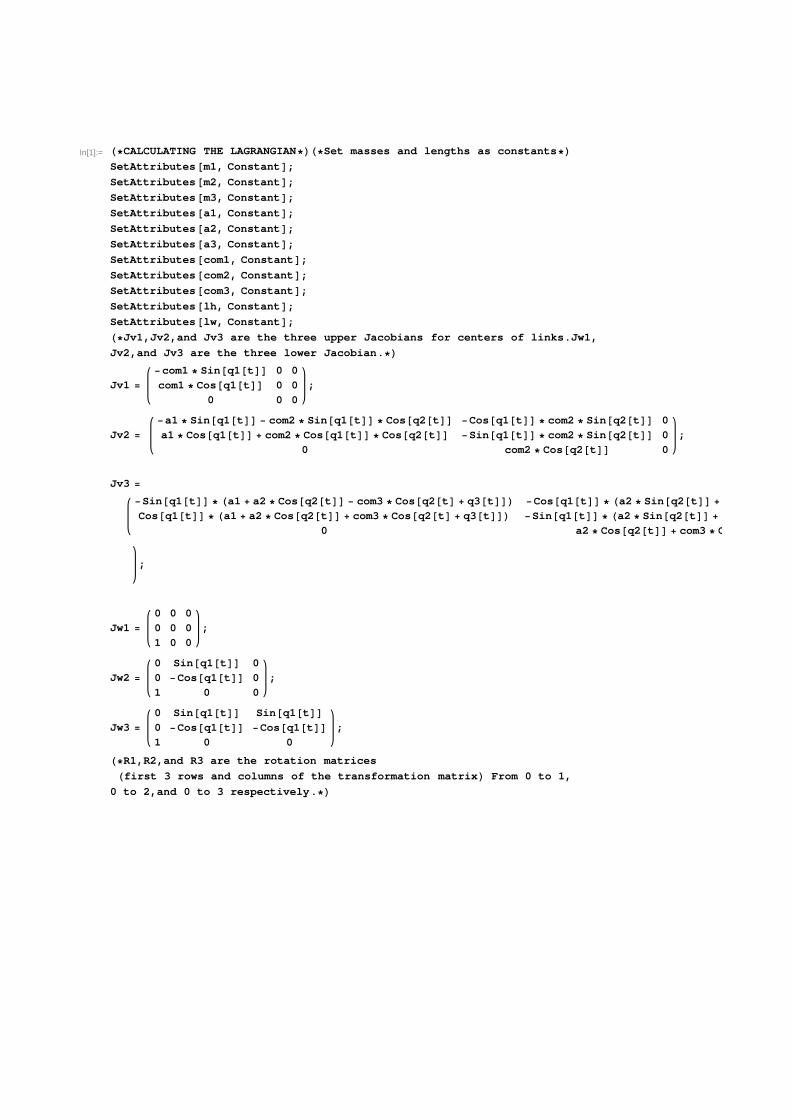
In[1]:= H*CALCULATING THE LAGRANGIAN*LH*Set masses and lengths as constants*LSetAttributes@m1, ConstantD;SetAttributes@m2, ConstantD;SetAttributes@m3, ConstantD;SetAttributes@a1, ConstantD;SetAttributes@a2, ConstantD;SetAttributes@a3, ConstantD;SetAttributes@com1, ConstantD;SetAttributes@com2, ConstantD;SetAttributes@com3, ConstantD;SetAttributes@lh, ConstantD;SetAttributes@lw, ConstantD;H*Jv1,Jv2,and Jv3 are the three upper Jacobians for centers of links.Jw1,

Jv2,and Jv3 are the three lower Jacobian.*L

Jv1 =

-com1 * Sin@q1@tDD 0 0

com1 * Cos@q1@tDD 0 0

0 0 0

;

Jv2 =

-a1 * Sin@q1@tDD - com2 * Sin@q1@tDD * Cos@q2@tDD -Cos@q1@tDD * com2 * Sin@q2@tDD 0

a1 * Cos@q1@tDD + com2 * Cos@q1@tDD * Cos@q2@tDD -Sin@q1@tDD * com2 * Sin@q2@tDD 0

0 com2 * Cos@q2@tDD 0

;

Jv3 =

-Sin@q1@tDD * Ha1 + a2 * Cos@q2@tDD - com3 * Cos@q2@tD + q3@tDDL -Cos@q1@tDD * Ha2 * Sin@q2@tDD +

Cos@q1@tDD * Ha1 + a2 * Cos@q2@tDD + com3 * Cos@q2@tD + q3@tDDL -Sin@q1@tDD * Ha2 * Sin@q2@tDD + com3

0 a2 * Cos@q2@tDD + com3 * Cos

;

Jw1 =

0 0 0

0 0 0

1 0 0

;

Jw2 =

0 Sin@q1@tDD 0

0 -Cos@q1@tDD 0

1 0 0

;

Jw3 =

0 Sin@q1@tDD Sin@q1@tDD0 -Cos@q1@tDD -Cos@q1@tDD1 0 0

;

H*R1,R2,and R3 are the rotation matrices

Hfirst 3 rows and columns of the transformation matrixL From 0 to 1,

0 to 2,and 0 to 3 respectively.*L

In[1]:=

R1 =

Cos@q1@tDD 0 Sin@q1@tDDSin@q1@tDD 0 -Cos@q1@tDD

0 1 0

;

R2 =

Cos@q1@tDD * Cos@q2@tDD -Cos@q1@tDD * Sin@q2@tDD Sin@q1@tDDSin@q1@tDD * Cos@q2@tDD -Sin@q1@tDD * Sin@q2@tDD -Cos@q1@tDD

Sin@q2@tDD Cos@q2@tDD 0

;

R3 =

Cos@q1@tDD * Cos@q2@tD + q3@tDD -Cos@q1@tDD * Sin@q3@tD + q2@tDD Sin@q1@tDDSin@q1@tDD * Cos@q2@tD + q3@tDD -Sin@q1@tDD * Sin@q3@tD + q2@tDD -Cos@q1@tDD

Sin@q2@tD + q3@tDD Cos@q2@tD + q3@tDD 0

;

H*I1,I2,and I3 are the inertia matrices of each of the links respectively. These

are all very rough estimates assuming each link is a rectangle with the

origin at the pin. lw is the link width and lh is the link height.*L

I1 =

Hlw^2 + lh^2L * m1 � 12 0 0

0 Ha1^2 + lw^2L * m1 � 12 0

0 0 Ha1^2 + lw^2L * m1 � 12

;

I2 =

Hlw^2 + lh^2L * m2 � 12 0 0

0 Hlh^2 + a2^2L * m2 � 12 0

0 0 Ha2^2 + lh^2L * m2 � 12

;

I3 =

Hlw^2 + lh^2L * m3 � 12 0 0

0 Hlh^2 + a3^2L * m3 � 12 0

0 0 Ha3^2 + lh^2L * m3 � 12

;

H*The Kinetic energies for each link*LDk1 = m1 * HTranspose@Jv1D.Jv1L + Transpose@Jw1D.R1.I1.Transpose@R1D.Jw1;Dk2 = m2 * HTranspose@Jv2D.Jv2L + Transpose@Jw2D.R2.I2.Transpose@R2D.Jw2;Dk3 = m3 * HTranspose@Jv3D.Jv3L + Transpose@Jw3D.R3.I3.Transpose@R3D.Jw3;Dtot = Dk1 + Dk2 + Dk3;

H*The Potential energies for each link and g is gravity vector,

multiplied by the coordinates of the COM of each link*L

g =

0

0

-9.81

;

P1 = Transpose@gD.com1 * Cos@q1@tDDcom1 * Sin@q1@tDD

0

* m1;

P2 = Transpose@gD.Cos@q1@tDD * Ha1 + com2 * Cos@q2@tDDLSin@q1@tDD * Ha1 + com2 * Cos@q2@tDDL

com2 * Sin@q2@tDD* m2;

P3 = Transpose@gD.Cos@q1@tDD * Ha1 + a2 * Cos@q2@tDD + com3 * Cos@q2@tD + q3@tDDLSin@q1@tDD * Ha1 + a2 * Cos@q2@tDD + com3 * Cos@q2@tD + q3@tDDL

a2 * Sin@q2@tDD + com3 * Sin@q2@tD + q3@tDD* m3;

2 Lagrangian_Rev8.nb

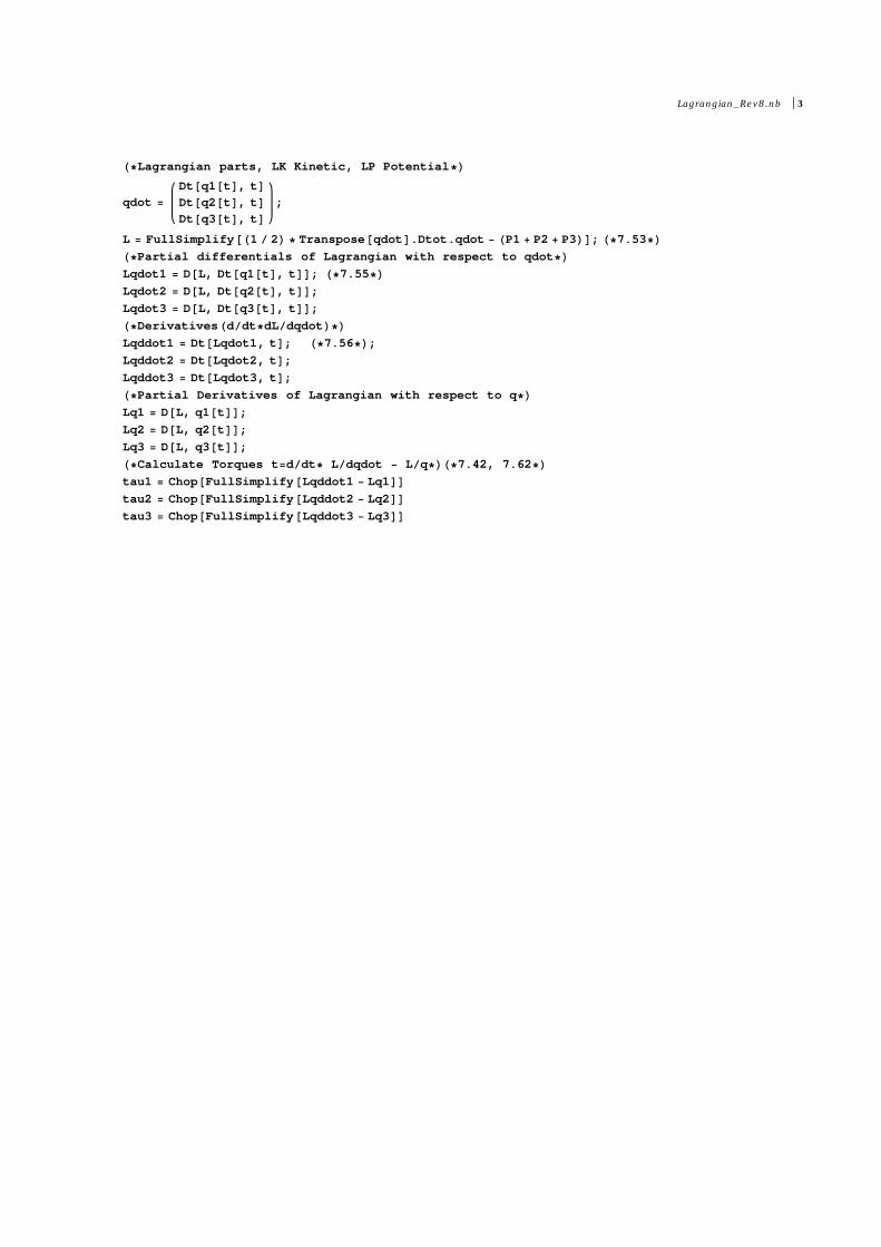
In[1]:=

H*Lagrangian parts, LK Kinetic, LP Potential*L

qdot =

Dt@q1@tD, tDDt@q2@tD, tDDt@q3@tD, tD

;

L = FullSimplify@H1 � 2L * Transpose@qdotD.Dtot.qdot - HP1 + P2 + P3LD; H*7.53*LH*Partial differentials of Lagrangian with respect to qdot*LLqdot1 = D@L, Dt@q1@tD, tDD; H*7.55*LLqdot2 = D@L, Dt@q2@tD, tDD;Lqdot3 = D@L, Dt@q3@tD, tDD;H*DerivativesHd�dt*dL�dqdotL*LLqddot1 = Dt@Lqdot1, tD; H*7.56*L;Lqddot2 = Dt@Lqdot2, tD;Lqddot3 = Dt@Lqdot3, tD;H*Partial Derivatives of Lagrangian with respect to q*LLq1 = D@L, q1@tDD;Lq2 = D@L, q2@tDD;Lq3 = D@L, q3@tDD;H*Calculate Torques t=d�dt* L�dqdot - L�q*LH*7.42, 7.62*Ltau1 = Chop@FullSimplify@Lqddot1 - Lq1DDtau2 = Chop@FullSimplify@Lqddot2 - Lq2DDtau3 = Chop@FullSimplify@Lqddot3 - Lq3DD

Lagrangian_Rev8.nb 3

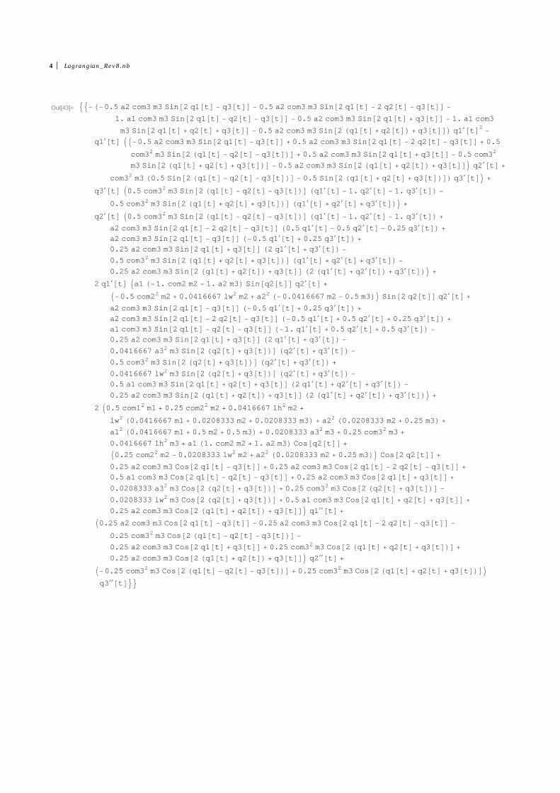
Out[43]= 99-H-0.5 a2 com3 m3 Sin@2 q1@tD - q3@tDD - 0.5 a2 com3 m3 Sin@2 q1@tD - 2 q2@tD - q3@tDD -

1. a1 com3 m3 Sin@2 q1@tD - q2@tD - q3@tDD - 0.5 a2 com3 m3 Sin@2 q1@tD + q3@tDD - 1. a1 com3

m3 Sin@2 q1@tD + q2@tD + q3@tDD - 0.5 a2 com3 m3 Sin@2 Hq1@tD + q2@tDL + q3@tDDL q1¢@tD2-

q1¢@tD II-0.5 a2 com3 m3 Sin@2 q1@tD - q3@tDD + 0.5 a2 com3 m3 Sin@2 q1@tD - 2 q2@tD - q3@tDD + 0.5

com32 m3 Sin@2 Hq1@tD - q2@tD - q3@tDLD + 0.5 a2 com3 m3 Sin@2 q1@tD + q3@tDD - 0.5 com32

m3 Sin@2 Hq1@tD + q2@tD + q3@tDLD - 0.5 a2 com3 m3 Sin@2 Hq1@tD + q2@tDL + q3@tDDM q2¢@tD +

com32 m3 H0.5 Sin@2 Hq1@tD - q2@tD - q3@tDLD - 0.5 Sin@2 Hq1@tD + q2@tD + q3@tDLDL q3¢@tDM +

q3¢@tD I0.5 com32 m3 Sin@2 Hq1@tD - q2@tD - q3@tDLD Hq1¢@tD - 1. q2¢@tD - 1. q3¢@tDL -

0.5 com32 m3 Sin@2 Hq1@tD + q2@tD + q3@tDLD Hq1¢@tD + q2¢@tD + q3¢@tDLM +

q2¢@tD I0.5 com32 m3 Sin@2 Hq1@tD - q2@tD - q3@tDLD Hq1¢@tD - 1. q2¢@tD - 1. q3¢@tDL +

a2 com3 m3 Sin@2 q1@tD - 2 q2@tD - q3@tDD H0.5 q1¢@tD - 0.5 q2¢@tD - 0.25 q3¢@tDL +

a2 com3 m3 Sin@2 q1@tD - q3@tDD H-0.5 q1¢@tD + 0.25 q3¢@tDL +

0.25 a2 com3 m3 Sin@2 q1@tD + q3@tDD H2 q1¢@tD + q3¢@tDL -

0.5 com32 m3 Sin@2 Hq1@tD + q2@tD + q3@tDLD Hq1¢@tD + q2¢@tD + q3¢@tDL -

0.25 a2 com3 m3 Sin@2 Hq1@tD + q2@tDL + q3@tDD H2 Hq1¢@tD + q2¢@tDL + q3¢@tDLM +

2 q1¢@tD Ia1 H-1. com2 m2 - 1. a2 m3L Sin@q2@tDD q2¢@tD +

I-0.5 com22 m2 + 0.0416667 lw2 m2 + a22 H-0.0416667 m2 - 0.5 m3LM Sin@2 q2@tDD q2¢@tD +

a2 com3 m3 Sin@2 q1@tD - q3@tDD H-0.5 q1¢@tD + 0.25 q3¢@tDL +

a2 com3 m3 Sin@2 q1@tD - 2 q2@tD - q3@tDD H-0.5 q1¢@tD + 0.5 q2¢@tD + 0.25 q3¢@tDL +

a1 com3 m3 Sin@2 q1@tD - q2@tD - q3@tDD H-1. q1¢@tD + 0.5 q2¢@tD + 0.5 q3¢@tDL -

0.25 a2 com3 m3 Sin@2 q1@tD + q3@tDD H2 q1¢@tD + q3¢@tDL -

0.0416667 a32 m3 Sin@2 Hq2@tD + q3@tDLD Hq2¢@tD + q3¢@tDL -

0.5 com32 m3 Sin@2 Hq2@tD + q3@tDLD Hq2¢@tD + q3¢@tDL +

0.0416667 lw2 m3 Sin@2 Hq2@tD + q3@tDLD Hq2¢@tD + q3¢@tDL -

0.5 a1 com3 m3 Sin@2 q1@tD + q2@tD + q3@tDD H2 q1¢@tD + q2¢@tD + q3¢@tDL -

0.25 a2 com3 m3 Sin@2 Hq1@tD + q2@tDL + q3@tDD H2 Hq1¢@tD + q2¢@tDL + q3¢@tDLM +

2 I0.5 com12 m1 + 0.25 com22 m2 + 0.0416667 lh2 m2 +

lw2 H0.0416667 m1 + 0.0208333 m2 + 0.0208333 m3L + a22 H0.0208333 m2 + 0.25 m3L +

a12 H0.0416667 m1 + 0.5 m2 + 0.5 m3L + 0.0208333 a32 m3 + 0.25 com32 m3 +

0.0416667 lh2 m3 + a1 H1. com2 m2 + 1. a2 m3L Cos@q2@tDD +

I0.25 com22 m2 - 0.0208333 lw2 m2 + a22 H0.0208333 m2 + 0.25 m3LM Cos@2 q2@tDD +

0.25 a2 com3 m3 Cos@2 q1@tD - q3@tDD + 0.25 a2 com3 m3 Cos@2 q1@tD - 2 q2@tD - q3@tDD +

0.5 a1 com3 m3 Cos@2 q1@tD - q2@tD - q3@tDD + 0.25 a2 com3 m3 Cos@2 q1@tD + q3@tDD +

0.0208333 a32 m3 Cos@2 Hq2@tD + q3@tDLD + 0.25 com32 m3 Cos@2 Hq2@tD + q3@tDLD -

0.0208333 lw2 m3 Cos@2 Hq2@tD + q3@tDLD + 0.5 a1 com3 m3 Cos@2 q1@tD + q2@tD + q3@tDD +

0.25 a2 com3 m3 Cos@2 Hq1@tD + q2@tDL + q3@tDDM q1¢¢@tD +

I0.25 a2 com3 m3 Cos@2 q1@tD - q3@tDD - 0.25 a2 com3 m3 Cos@2 q1@tD - 2 q2@tD - q3@tDD -

0.25 com32 m3 Cos@2 Hq1@tD - q2@tD - q3@tDLD -

0.25 a2 com3 m3 Cos@2 q1@tD + q3@tDD + 0.25 com32 m3 Cos@2 Hq1@tD + q2@tD + q3@tDLD +

0.25 a2 com3 m3 Cos@2 Hq1@tD + q2@tDL + q3@tDDM q2¢¢@tD +

I-0.25 com32 m3 Cos@2 Hq1@tD - q2@tD - q3@tDLD + 0.25 com32 m3 Cos@2 Hq1@tD + q2@tD + q3@tDLDMq3¢¢@tD==

4 Lagrangian_Rev8.nb

Out[44]= 99H-9.81 com2 m2 - 9.81 a2 m3L Cos@q2@tDD - 9.81 com3 m3 Cos@q2@tD + q3@tDD +

I1. a1 com2 m2 Sin@q2@tDD + 1. a1 a2 m3 Sin@q2@tDD + 0.0416667 a22 m2 Sin@2 q2@tDD +

0.5 com22 m2 Sin@2 q2@tDD - 0.0416667 lw2 m2 Sin@2 q2@tDD + 0.5 a22 m3 Sin@2 q2@tDD -

0.5 a2 com3 m3 Sin@2 q1@tD - q3@tDD + 0.5 com32 m3 Sin@2 Hq1@tD - q2@tD - q3@tDLD -

0.5 a1 com3 m3 Sin@2 q1@tD - q2@tD - q3@tDD + 0.5 a2 com3 m3 Sin@2 q1@tD + q3@tDD +

0.0416667 a32 m3 Sin@2 Hq2@tD + q3@tDLD + 0.5 com32 m3 Sin@2 Hq2@tD + q3@tDLD -

0.0416667 lw2 m3 Sin@2 Hq2@tD + q3@tDLD - 0.5 com32 m3 Sin@2 Hq1@tD + q2@tD + q3@tDLD +

0.5 a1 com3 m3 Sin@2 q1@tD + q2@tD + q3@tDDM q1¢@tD2+

H0.25 a2 com3 m3 Sin@2 q1@tD - q3@tDD - 0.25 a2 com3 m3 Sin@2 q1@tD - 2 q2@tD - q3@tDD +

0.25 a2 com3 m3 Sin@2 q1@tD + q3@tDD - 0.25 a2 com3 m3 Sin@2 Hq1@tD + q2@tDL + q3@tDDLq1¢@tD q3¢@tD - 2. a2 com3 m3 Sin@q3@tDD q2¢@tD q3¢@tD -

1. a2 com3 m3 Sin@q3@tDD q3¢@tD2+ 0.25 a2 com3 m3 Cos@2 q1@tD - q3@tDD q1¢¢@tD -

0.25 a2 com3 m3 Cos@2 q1@tD - 2 q2@tD - q3@tDD q1¢¢@tD -

0.25 com32 m3 Cos@2 Hq1@tD - q2@tD - q3@tDLD q1¢¢@tD -

0.25 a2 com3 m3 Cos@2 q1@tD + q3@tDD q1¢¢@tD +

0.25 com32 m3 Cos@2 Hq1@tD + q2@tD + q3@tDLD q1¢¢@tD +

0.25 a2 com3 m3 Cos@2 Hq1@tD + q2@tDL + q3@tDD q1¢¢@tD +

0.0833333 a22 m2 q2¢¢@tD + 1. com22 m2 q2¢¢@tD + 0.0833333 lh2 m2 q2¢¢@tD +

1. a22 m3 q2¢¢@tD + 0.0833333 a32 m3 q2¢¢@tD + 1. com32 m3 q2¢¢@tD +

0.0833333 lh2 m3 q2¢¢@tD + 2. a2 com3 m3 Cos@q3@tDD q2¢¢@tD +

0.0833333 a32 m3 q3¢¢@tD + 1. com32 m3 q3¢¢@tD +

0.0833333 lh2 m3 q3¢¢@tD + 1. a2 com3 m3 Cos@q3@tDD q3¢¢@tD==

Out[45]= 99-9.81 com3 m3 Cos@q2@tD + q3@tDD +

I-0.25 a2 com3 m3 Sin@2 q1@tD - q3@tDD - 0.25 a2 com3 m3 Sin@2 q1@tD - 2 q2@tD - q3@tDD +

0.5 com32 m3 Sin@2 Hq1@tD - q2@tD - q3@tDLD - 0.5 a1 com3 m3 Sin@2 q1@tD - q2@tD - q3@tDD +

0.25 a2 com3 m3 Sin@2 q1@tD + q3@tDD + 0.0416667 a32 m3 Sin@2 Hq2@tD + q3@tDLD +

0.5 com32 m3 Sin@2 Hq2@tD + q3@tDLD - 0.0416667 lw2 m3 Sin@2 Hq2@tD + q3@tDLD -

0.5 com32 m3 Sin@2 Hq1@tD + q2@tD + q3@tDLD + 0.5 a1 com3 m3 Sin@2 q1@tD + q2@tD + q3@tDD +

0.25 a2 com3 m3 Sin@2 Hq1@tD + q2@tDL + q3@tDDM q1¢@tD2+

H-0.25 a2 com3 m3 Sin@2 q1@tD - q3@tDD + 0.25 a2 com3 m3 Sin@2 q1@tD - 2 q2@tD - q3@tDD -

0.25 a2 com3 m3 Sin@2 q1@tD + q3@tDD + 0.25 a2 com3 m3 Sin@2 Hq1@tD + q2@tDL + q3@tDDLq1¢@tD q2¢@tD + 1. a2 com3 m3 Sin@q3@tDD q2¢@tD2

-

0.25 com32 m3 Cos@2 Hq1@tD - q2@tD - q3@tDLD q1¢¢@tD +

0.25 com32 m3 Cos@2 Hq1@tD + q2@tD + q3@tDLD q1¢¢@tD +

0.0833333 a32 m3 q2¢¢@tD + 1. com32 m3 q2¢¢@tD + 0.0833333 lh2 m3 q2¢¢@tD +

1. a2 com3 m3 Cos@q3@tDD q2¢¢@tD + 0.0833333 a32 m3 q3¢¢@tD +

1. com32 m3 q3¢¢@tD + 0.0833333 lh2 m3 q3¢¢@tD==

Lagrangian_Rev8.nb 5

Appendix B

Appendix B: Symbolic MatlabScripts

function tau=NewLagrangian(k)

%Script to calculate Lagrangian

%Define symbolic variables:

syms q1 q2 q3 q1dot q2dot q3dot q1ddot q2ddot q3ddot real

syms a1 a2 a3 m1 m2 m3 lw lh real

q = [q1; q2; q3];

%Define trigonometric functions

s1=sin(q1);

s2=sin(q2);

s3=sin(q3);

c1=cos(q1);

c2=cos(q2);

c3=cos(q3);

s23=sin(q2+q3);

c23=cos(q2+q3);

%Define constant

g=9.81;

%Define Jacobians for centers of Mass

Jcv1=[-(a1/2)*s1 0 0; (a1/2) 0 0; 0 0 0];

Jcv2=[-a1*s1-(a2/2)*s1*c2 -c1*(a2/2)*s2 0;

a1*c1+(a2/2)*c1*c2 -s1*(a2/2)*s2 0;

0 (a2/2)*c2 0];

Jcv3=[-a1*s1-a2*s1*c2-(a3/2)*s1*c23 -c1*(a2*s2+(a3/2)*s23) -c1*(a3/2)*s23;

a1*c1+a2*c1*c2+(a3/2)*c1*c23 -s1*(a2*s2*(a3/2)*s23) -s1*(a2/2)*s23;

72

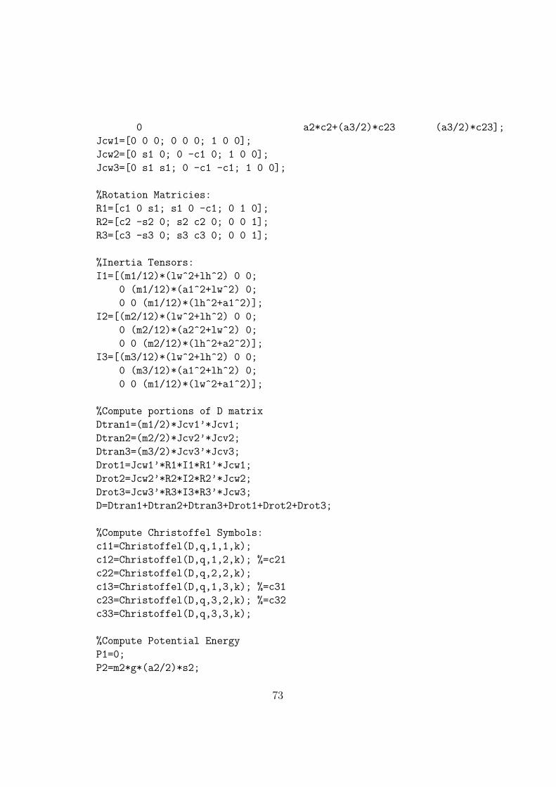
0 a2*c2+(a3/2)*c23 (a3/2)*c23];

Jcw1=[0 0 0; 0 0 0; 1 0 0];

Jcw2=[0 s1 0; 0 -c1 0; 1 0 0];

Jcw3=[0 s1 s1; 0 -c1 -c1; 1 0 0];

%Rotation Matricies:

R1=[c1 0 s1; s1 0 -c1; 0 1 0];

R2=[c2 -s2 0; s2 c2 0; 0 0 1];

R3=[c3 -s3 0; s3 c3 0; 0 0 1];

%Inertia Tensors:

I1=[(m1/12)*(lw^2+lh^2) 0 0;

0 (m1/12)*(a1^2+lw^2) 0;

0 0 (m1/12)*(lh^2+a1^2)];

I2=[(m2/12)*(lw^2+lh^2) 0 0;

0 (m2/12)*(a2^2+lw^2) 0;

0 0 (m2/12)*(lh^2+a2^2)];

I3=[(m3/12)*(lw^2+lh^2) 0 0;

0 (m3/12)*(a1^2+lh^2) 0;

0 0 (m1/12)*(lw^2+a1^2)];

%Compute portions of D matrix

Dtran1=(m1/2)*Jcv1’*Jcv1;

Dtran2=(m2/2)*Jcv2’*Jcv2;

Dtran3=(m3/2)*Jcv3’*Jcv3;

Drot1=Jcw1’*R1*I1*R1’*Jcw1;

Drot2=Jcw2’*R2*I2*R2’*Jcw2;

Drot3=Jcw3’*R3*I3*R3’*Jcw3;

D=Dtran1+Dtran2+Dtran3+Drot1+Drot2+Drot3;

%Compute Christoffel Symbols:

c11=Christoffel(D,q,1,1,k);

c12=Christoffel(D,q,1,2,k); %=c21

c22=Christoffel(D,q,2,2,k);

c13=Christoffel(D,q,1,3,k); %=c31

c23=Christoffel(D,q,3,2,k); %=c32

c33=Christoffel(D,q,3,3,k);

%Compute Potential Energy

P1=0;

P2=m2*g*(a2/2)*s2;

73

P3=m3*g*a2*s2+(a3/2)*s23;

P=P1+P2+P3;

%Compute gravity factor:

g=diff(P,q(k));

%Finally, compute torque:

tau=D(k,1)*q1ddot+D(k,2)*q2ddot+D(k,3)*q3ddot ...

+ c11*q1dot^2+2*c12*q1dot*q2dot+c22*q2dot^2 ...

+ 2*c13*q1dot*q3dot+2*c23*q2dot*q3dot+c33*q3dot^2+g;

function c=Christoffel(D,q,i,j,k)

c=(1/2)*(diff(D(k,j),q(i))+diff(D(k,i),q(j))-diff(D(i,j),q(k)));

74

Appendix C

Appendix C: Matlab Files forode45 Solver andSingularity/ManipulabilityCheck

%%%%%%%%%%%%%%%%%%%%%%%%%%%%%

% domodel.m %

% By KG Youngsma %

% Date: May 14, 2012 %

% Rev 1 Working wo Control %

%%%%%%%%%%%%%%%%%%%%%%%%%%%%%

%Description: This script is the central "do" file for all the other functions that make up the model for

%the three DoF robotic leg. It requires:

% -threedoflegrev2.m (the file used for ode45, this calculates real joint positions, velocities, and acclerations based on desired torques)

% -EulerLagrange.m (The file which calculates torques based on desired joint position, velocities, and acclerations)

% -trajectory.m (The file which creates a trajectory of joint positions based on global coordinate set points)

% -invkin.m (Calculates inverse kinematics)

% -quintic.m (Generates the quintic path for desired joint

% positions, velocities, and accelerations)

%This do file also hosts the following variables, which are also pasted

%into every function called by this script:

%Physical Constants:

%Link Lengths in meters

a1=0.08;

75

a2=0.2;

a3=0.2;

%Link Masses in kilograms

m1=1;

m2=1;

m3=1;

%Link width and height (for inertia matricies) in meters

lw=0.06;

lh=0.06;

%Gravity:

g=9.81;

%Trajectory Constants: Define lift, swing, and set times and positions, in

%which the step begins and ends with set, lift is end of the "lift" phase,

%and swing is at the end of the swing phase.

xset=-0.15;

yset=0.1;

zset=-0.3;

tset=0;

xlift=0;

ylift=0.16;

zlift=-0.1;

tlift=25;

xswing=0.15;

yswing=0.1;

zswing=-0.3;

tswing=50;

tend=100;

%Prior to runtime for the ode45 solver, all desired torques are calculated for the single step.

%Aquire all joint positions, velocities, and accelerations:

qlift=trajectory(tset,xset,yset,zset,tlift,xlift,ylift,zlift);

qswing=trajectory(tlift,xlift,ylift,zlift,tswing,xswing,yswing,zswing);

qset=trajectory(tswing,xswing,yswing,zswing,tend,xset,yset,zset);

%Assemble matrix of columns of all desired joint positions, velocities, and accelerations in rows of t:

qpva=zeros(9,100);

for t = 1:100

if t<=25 && t>0,

76

qpva(:,t)=qlift(:,t);

elseif t<=50 && t>25

qpva(:,t)=qswing(:,(t-25));

else

qpva(:,t)=qset(:,(t-50));

end

end

%Plot Desired Results:

subplot(3,3,1); plot(qpva(1,:)); title(’Joint 1 Desired’); xlabel(’Time’); ylabel(’Position in Radians’);

subplot(3,3,2); plot(qpva(2,:)); title(’Joint 2 Desired’); xlabel(’Time’); ylabel(’Position in Radians’);

subplot(3,3,3); plot(qpva(3,:)); title(’Joint 3 Desired’); xlabel(’Time’); ylabel(’Position in Radians’);

subplot(3,3,4); plot(qpva(4,:)); title(’Joint 1 Desired’); xlabel(’Time’); ylabel(’Velocity in Radians per Second’);

subplot(3,3,5); plot(qpva(5,:)); title(’Joint 2 Desired’); xlabel(’Time’); ylabel(’Velocity in Radians per Second’);

subplot(3,3,6); plot(qpva(6,:)); title(’Joint 3 Desired’); xlabel(’Time’); ylabel(’Velocity in Radians per Second’);

subplot(3,3,7); plot(qpva(7,:)); title(’Joint 1 Desired’); xlabel(’Time’); ylabel(’Acceleration in Radians per Second Squared’);

subplot(3,3,8); plot(qpva(8,:)); title(’Joint 2 Desired’); xlabel(’Time’); ylabel(’Acceleration in Radians per Second Squared’);

subplot(3,3,9); plot(qpva(9,:)); title(’Joint 3 Desired’); xlabel(’Time’); ylabel(’Acceleration in Radians per Second Squared’);

hold on

%Define tau matrix and results:

tau=zeros(100,3);

qresult=[];

time=[];

%Begin ode45 loop, where torque is input every second

for t=1:100

%Set initial joint positions and velocities, where

%q=[q1; q2; q3; q1dot; q2dot; q3dot]

qin=qpva(1:6,t);

%Use Euler-Lagrange to calculate torque

tau=EulerLagrange(qpva(:,t));

%Run ode45 using the threedofleg m file

[t,qout] = ode45(@(t,q) threedoflegrev2(t,q,tau),[t t+1],qin);

%Collect Results:

%time=vertcat(time,t);

qresult=vertcat(qresult,qout);

end

%Plot results:

subplot(3,3,1); plot(qresult(:,1),’-r’); %title(’Joint 1 Results’); xlabel(’Time’); ylabel(’Position in Radians’);

subplot(3,3,2); plot(qresult(:,2),’-r’); %title(’Joint 2 Results’); xlabel(’Time’); ylabel(’Position in Radians’);

77

subplot(3,3,3); plot(qresult(:,3),’-r’); %title(’Joint 3 Results’); xlabel(’Time’); ylabel(’Position in Radians’);

subplot(3,3,4); plot(qresult(:,4),’-r’); %title(’Joint 1 Results’); xlabel(’Time’); ylabel(’Velocity in Radians per Second’);

subplot(3,3,5); plot(qresult(:,5),’-r’); %title(’Joint 2 Results’); xlabel(’Time’); ylabel(’Velocity in Radians per Second’);

subplot(3,3,6); plot(qresult(:,6),’-r’); %title(’Joint 3 Results’); xlabel(’Time’); ylabel(’Velocity in Radians per Second’);

%%%%%%%%%%%%%%%%%%%%%%%%%%%%%%%%%%%%%%%%%%%%%%%%%%%%%%%%%%%%%%%%%

% 3doflegrev2.m %Influenced by the the file robot.m %

% By KG Youngsma % by Nicholas Alunni %

% Date: April 18, 2012 % Tim Flynn %

% Rev 2 Draft % Vadim Chernyak %

%%%%%%%%%%%%%%%%%%%%%%%%%%%% Ennio Claretti %

% Paul Heslinga %

%%%%%%%%%%%%%%%%%%%%%%%%%%%%%%%%%%%%%%

function qdot=threedoflegrev2(t,q,tau)

%Description: This function sets out the differential equation to be solved by the do file.

%It returns actual joint position, velocity, and acceration based on initial joint position and velocity and desired torques.

%Inputs: tau1, tau2, tau3, three tau values.

%Input initial condition variables

%Vector of q’s

q1=q(1);

q2=q(2);

q3=q(3);

q1dot=q(4);

q2dot=q(5);

q3dot=q(6);

%Define trigonometric functions

s1=sin(q1);

s2=sin(q2);

s3=sin(q3);

c1=cos(q1);

c2=cos(q2);

c3=cos(q3);

s23=sin(q2+q3);

c23=cos(q2+q3);

78

%Physical Constants:

%Link Lengths in meters

a1=0.08;

a2=0.2;

a3=0.2;

%Link Masses in kilograms

m1=1;

m2=1;

m3=1;

%Link width and height (for inertia matricies) in meters

lw=0.06;

lh=0.06;

%Gravity:

g=9.81;

%%Dynamic Model

%Define Jacobians for centers of Mass

Jcv1=[-(a1/2)*s1 0 0; (a1/2)*c1 0 0; 0 0 0];

Jcv2=[-a1*s1-(a2/2)*s1*c2 -c1*(a2/2)*s2 0;

a1*c1+(a2/2)*c1*c2 -s1*(a2/2)*s2 0;

0 (a2/2)*c2 0];

Jcv3=[-a1*s1-a2*s1*c2-(a3/2)*s1*c23 -c1*(a2*s2+(a3/2)*s23) -c1*(a3/2)*s23;

a1*c1+a2*c1*c2+(a3/2)*c1*c23 -s1*(a2*s2*(a3/2)*s23) -s1*(a2/2)*s23;

0 a2*c2+(a3/2)*c23 (a3/2)*c23];

Jcw1=[0 0 0; 0 0 0; 1 0 0];

Jcw2=[0 s1 0; 0 -c1 0; 1 0 0];

Jcw3=[0 s1 s1; 0 -c1 -c1; 1 0 0];

%Rotation Matricies: orientation transformation from "the body attached frame and the inertial frame"

R1=[c1 0 s1; s1 0 -c1; 0 1 0];

R2=[c1*c2 -c1*s2 s1; s1*c2 -s1*s2 -c1; s2 c2 0];

R3=[c1*c23 -c1*s23 s1; s1*c23 -s1*s23 -c1; s23 c23 0];

%Inertia Tensors:

I1=[(m1/12)*(lw^2+lh^2) 0 0;

0 (m1/12)*(a1^2+lw^2) 0;

0 0 (m1/12)*(lh^2+a1^2)];

I2=[(m2/12)*(lw^2+lh^2) 0 0;

0 (m2/12)*(a2^2+lw^2) 0;

0 0 (m2/12)*(lh^2+a2^2)];

I3=[(m3/12)*(lw^2+lh^2) 0 0;

79

0 (m3/12)*(a3^2+lh^2) 0;

0 0 (m3/12)*(lw^2+a3^2)];

%Compute portions of D matrix

Dtran1=(m1/2)*Jcv1’*Jcv1;

Dtran2=(m2/2)*Jcv2’*Jcv2;

Dtran3=(m3/2)*Jcv3’*Jcv3;

Drot1=Jcw1’*R1*I1*R1’*Jcw1;

Drot2=Jcw2’*R2*I2*R2’*Jcw2;

Drot3=Jcw3’*R3*I3*R3’*Jcw3;

D=Dtran1+Dtran2+Dtran3+Drot1+Drot2+Drot3;

%Compute C Matrix (from Mathematica);

c11=c1*(-0.032*c23*s1-0.08*c2*c23*s1)*q1dot+(-0.00151667*sin(2*q2)-0.00303333*sin(2*(q2+q3))+c1^2*(-0.024*s2-0.025* sin(2*q2)-0.01*s3-0.016*s23-0.01*sin(2*(q2+q3))-0.03*sin(2*q2+q3))+s1^2*(-0.024*s2-0.025*sin(2*q2)+0.01*s3+0.016*s23-0.01*sin(2*(q2+q3))+0.03*sin(2*q2+q3)))*q2dot;

c12=(-0.00151667*sin(2*q2)-0.00151667*sin(2*(q2+q3))+c1^2*(-0.024*s2-0.025*sin(2*q2)-0.008*sin(q2+q3)-0.005*sin(2* (q2+q3))-0.02*sin(2*q2+q3))+s1^2*(-0.024*s2-0.025*sin(2*q2)+0.008*s23-0.005*sin(2*(q2+q3))+0.02*sin(2*q2+q3)))*q1dot+(c1*(-0.04*c2*c23*s1-0.04*c23^2*s1)+sin(2*q1)*(0.03*s2*s23+0.02*s23^2))*q2dot;

c13=((c1^2*(-0.008-0.02*c2-0.01*c23)+(0.008+0.02*c2)*s1^2)*s23+(-0.00151667-0.005*s1^2)*sin(2*(q2+q3)))*q1dot+(-0.04*c1*c23^2*s1+sin(2*q1)*(0.01*s2+0.02*s23)*s23)*q2dot;

c21=(0.00151667*sin(2*q2)+c1^2*(0.024*s2+0.025*sin(2*q2)+0.02*s3+0.008*s23-0.005*sin(2*(q2+q3)))+s1^2*(0.024*s2+0.025*sin(2*q2)-0.02*s3-0.008*s23+0.015*sin(2*(q2+q3)))+0.00151667*sin(2*(q2+q3)))*q1dot+0.01*sin(2*q1)*s2*s23*q2dot;

c22=-0.02*s3*q2dot;

c23=0.01*sin(2*q1)*s2*s23*q1dot+(-0.04*c2*s23+c23*(0.04*s2+0.02*c1^2*s23)+(-0.01+0.01*s1^2)*sin(2*(q2+q3)))*q2dot;

c31=((c1^2*(0.008+0.02*c2-0.01*c23)+(-0.008-0.02*c2)*s1^2)*s23+(0.00151667+0.015*s1^2)*sin(2*(q2+q3)))*q1dot-0.01* sin(2*q1)*s2*s23*q2dot;

c32=-0.01*sin(2*q1)*s2*s23*q1dot+(0.02*c2*s23+c23*(-0.02*s2+0.02*c1^2*s23)+(-0.01+0.01*s1^2)*sin(2*(q2+q3)))*q2dot;

c33=(0.01*c1^2*sin(2*(q2+q3))+(-0.01+0.01*s1^2)*sin(2*(q2+q3)))*q2dot;

C=[c11 c12 c13; c21 c22 c23; c31 c32 c33];

%Compute gravity matrix:

g1=0;

g2=0.981*c2+9.81*(0.2*c2+0.1*c23);

g3=0.981*c23;

G=[g1; g2; g3];

% Calculate Velocities and Accelerations

qdot = [0;0;0;0;0;0];

% Calculating Accelerations Here, using input tau:

A = D\(tau - C*[q1dot; q2dot; q3dot] - G);

%%%%%%%%%%%%%%%%%%%%%%%%%%%%%

% EulerLagrange.m %

% By KG Youngsma %

80

% Date: April 16, 2012 %

% Rev 0 Draft %

%%%%%%%%%%%%%%%%%%%%%%%%%%%%%

function tau=EulerLagrange(qall)

%Description: Function to calculate torque based on joint position, velocity, and accleration for a single joint

%Break up inputs:

q1=qall(1);

q2=qall(2);

q3=qall(3);

q1dot=qall(4);

q2dot=qall(5);

q3dot=qall(6);

q1ddot=qall(7);

q2ddot=qall(8);

q3ddot=qall(9);

%Physical Constants:

%Link Lengths in meters

a1=0.08;

a2=0.2;

a3=0.2;

%Link Masses in kilograms

m1=1;

m2=1;

m3=1;

%Link width and height (for inertia matricies) in meters

lw=0.06;

lh=0.06;

%Gravity:

g=9.81;

%Define trigonometric functions

s1=sin(q1);

s2=sin(q2);

s3=sin(q3);

c1=cos(q1);

c2=cos(q2);

c3=cos(q3);

81

s23=sin(q2+q3);

c23=cos(q2+q3);

%Define Jacobians for centers of Mass

Jcv1=[-(a1/2)*s1 0 0; (a1/2)*c1 0 0; 0 0 0];

Jcv2=[-a1*s1-(a2/2)*s1*c2 -c1*(a2/2)*s2 0;

a1*c1+(a2/2)*c1*c2 -s1*(a2/2)*s2 0;

0 (a2/2)*c2 0];

Jcv3=[-a1*s1-a2*s1*c2-(a3/2)*s1*c23 -c1*(a2*s2+(a3/2)*s23) -c1*(a3/2)*s23;

a1*c1+a2*c1*c2+(a3/2)*c1*c23 -s1*(a2*s2*(a3/2)*s23) -s1*(a2/2)*s23;

0 a2*c2+(a3/2)*c23 (a3/2)*c23];

Jcw1=[0 0 0; 0 0 0; 1 0 0];

Jcw2=[0 s1 0; 0 -c1 0; 1 0 0];

Jcw3=[0 s1 s1; 0 -c1 -c1; 1 0 0];

%Rotation Matricies: orientation transformation from "the body attached frame and the inertial frame"

R1=[c1 0 s1; s1 0 -c1; 0 1 0];

R2=[c1*c2 -c1*s2 s1; s1*c2 -s1*s2 -c1; s2 c2 0];

R3=[c1*c23 -c1*s23 s1; s1*c23 -s1*s23 -c1; s23 c23 0];

%Inertia Tensors:

I1=[(m1/12)*(lw^2+lh^2) 0 0;

0 (m1/12)*(a1^2+lw^2) 0;

0 0 (m1/12)*(lh^2+a1^2)];

I2=[(m2/12)*(lw^2+lh^2) 0 0;

0 (m2/12)*(a2^2+lw^2) 0;

0 0 (m2/12)*(lh^2+a2^2)];

I3=[(m3/12)*(lw^2+lh^2) 0 0;

0 (m3/12)*(a3^2+lh^2) 0;

0 0 (m3/12)*(lw^2+a3^2)];

%Compute portions of D matrix (Equation 7.50):

Dtran1=(m1/2)*Jcv1’*Jcv1;

Dtran2=(m2/2)*Jcv2’*Jcv2;

Dtran3=(m3/2)*Jcv3’*Jcv3;

Drot1=Jcw1’*R1*I1*R1’*Jcw1;

Drot2=Jcw2’*R2*I2*R2’*Jcw2;

Drot3=Jcw3’*R3*I3*R3’*Jcw3;

D=Dtran1+Dtran2+Dtran3+Drot1+Drot2+Drot3;

%Compute C Matrix (from Mathematica);

82

c11=c1*(-0.032*c23*s1-0.08*c2*c23*s1)*q1dot+(-0.00151667*sin(2*q2)-0.00303333*sin(2*(q2+q3))+c1^2*(-0.024*s2-0.025* sin(2*q2)-0.01*s3-0.016*s23-0.01*sin(2*(q2+q3))-0.03*sin(2*q2+q3))+s1^2*(-0.024*s2-0.025*sin(2*q2)+0.01*s3+0.016*s23-0.01*sin(2*(q2+q3))+0.03*sin(2*q2+q3)))*q2dot;

c12=(-0.00151667*sin(2*q2)-0.00151667*sin(2*(q2+q3))+c1^2*(-0.024*s2-0.025*sin(2*q2)-0.008*sin(q2+q3)-0.005*sin(2* (q2+q3))-0.02*sin(2*q2+q3))+s1^2*(-0.024*s2-0.025*sin(2*q2)+0.008*s23-0.005*sin(2*(q2+q3))+0.02*sin(2*q2+q3)))*q1dot+(c1*(-0.04*c2*c23*s1-0.04*c23^2*s1)+sin(2*q1)*(0.03*s2*s23+0.02*s23^2))*q2dot;

c13=((c1^2*(-0.008-0.02*c2-0.01*c23)+(0.008+0.02*c2)*s1^2)*s23+(-0.00151667-0.005*s1^2)*sin(2*(q2+q3)))*q1dot+(-0.04*c1*c23^2*s1+sin(2*q1)*(0.01*s2+0.02*s23)*s23)*q2dot;

c21=(0.00151667*sin(2*q2)+c1^2*(0.024*s2+0.025*sin(2*q2)+0.02*s3+0.008*s23-0.005*sin(2*(q2+q3)))+s1^2*(0.024*s2+0.025*sin(2*q2)-0.02*s3-0.008*s23+0.015*sin(2*(q2+q3)))+0.00151667*sin(2*(q2+q3)))*q1dot+0.01*sin(2*q1)*s2*s23*q2dot;

c22=-0.02*s3*q2dot;

c23=0.01*sin(2*q1)*s2*s23*q1dot+(-0.04*c2*s23+c23*(0.04*s2+0.02*c1^2*s23)+(-0.01+0.01*s1^2)*sin(2*(q2+q3)))*q2dot;

c31=((c1^2*(0.008+0.02*c2-0.01*c23)+(-0.008-0.02*c2)*s1^2)*s23+(0.00151667+0.015*s1^2)*sin(2*(q2+q3)))*q1dot-0.01* sin(2*q1)*s2*s23*q2dot;

c32=-0.01*sin(2*q1)*s2*s23*q1dot+(0.02*c2*s23+c23*(-0.02*s2+0.02*c1^2*s23)+(-0.01+0.01*s1^2)*sin(2*(q2+q3)))*q2dot;

c33=(0.01*c1^2*sin(2*(q2+q3))+(-0.01+0.01*s1^2)*sin(2*(q2+q3)))*q2dot;

C=[c11 c12 c13; c21 c22 c23; c31 c32 c33];

%Compute gravity matrix:

g1=0;

g2=0.981*c2+9.81*(0.2*c2+0.1*c23);

g3=0.981*c23;

G=[g1; g2; g3];

%Finally, compute torques (Equation 7.63):

tau=D*[q1ddot; q2ddot; q3ddot]+C*[q1dot; q2dot; q3dot]+G;

%%%%%%%%%%%%%%%%%%%%%%%%%%%%%

% Trajectory.m %

% By KG Youngsma %

% Date: April 16, 2012 %

% Rev 0 Draft %

%%%%%%%%%%%%%%%%%%%%%%%%%%%%%

function qall=trajectory(t0,x0,y0,z0,tf,xf,yf,zf)

%Description: This function returns a quintic path of joint positions, velocities, and accelerations.

%Find the inverse kinematics of each beginning and end point:

q0s=invkin(x0,y0,z0);

qfs=invkin(xf,yf,zf);

%Get the quintic path of joint positions, velocities, and accelerations between each configuration:

q1pva=quintic(t0,q0s(1),tf,qfs(1));

q2pva=quintic(t0,q0s(2),tf,qfs(2));

q3pva=quintic(t0,q0s(3),tf,qfs(3));

83

%Assemble the qall array, placing each value in a different row and each time in a different column.

qall(1,:)=q1pva(1,:); %Row 1: Joint 1 series of positions

qall(2,:)=q2pva(1,:); %Row 2: Joint 2 series of positions

qall(3,:)=q3pva(1,:); %Joint 3 series of positions

qall(4,:)=q1pva(2,:); %Joint 1 series of velocities

qall(5,:)=q2pva(2,:); %Joint 2 series of velocities

qall(6,:)=q3pva(2,:); %Joint 3 series of velocities

qall(7,:)=q1pva(3,:); %Joint 1 series of accelerations

qall(8,:)=q2pva(3,:); %Row 8: Joint 2 series of accelerations

qall(9,:)=q3pva(3,:); %Row 9: Joint 3 series of accelerations

%%%%%%%%%%%%%%%%%%%%%%%%%%%%%

% quintic.m %

% By KG Youngsma %

% Date: April 16, 2012 %

% Rev 0 Draft %

%%%%%%%%%%%%%%%%%%%%%%%%%%%%%

function qpva=quintic(t0,q0,tf,qf)

%Description: Returns the quintic polynomial path of joint positions, velocities, and accelerations between the two joint positions:

v0=0;

a0=0;

vf=0;

af=0;

%Set up the matrix:

Matrix = [1 t0 t0^2 t0^3 t0^4 t0^5;

0 1 2*t0 3*t0^2 4*t0^3 5*t0^4;

0 0 2 6*t0 12*t0^2 20*t0^3;

1 tf tf^2 tf^3 tf^4 tf^5;

0 1 2*tf 3*tf^2 4*tf^3 5*tf^4;

0 0 2 6*tf 12*tf^2 20*tf^3];

%The column vector of givens:

Given = [q0; v0; a0; qf; vf; af];

%Solve for a set of constants in matrix a to feed back into position,

%velocity and accelerations over time.

A = inv(Matrix)*Given;

%Return position, velocity, and acceleration trajectory over time.

%Set up loop and matrices for return:

84

i = 1;

length=tf-t0;

qpva = zeros(3,length);

for t = t0:tf

qpva(1,i) = [1 t t^2 t^3 t^4 t^5]*A;

qpva(2,i) = [0 1 2*t 3*t^2 4*t^3 5*t^4]*A;

qpva(3,i) = [0 0 2 6*t 12*t^2 20*t^3]*A;

i = i + 1;

end

%%%%%%%%%%%%%%%%%%%%%%%%%%%%%%%%%%%%%%%%

% invkin.m %

% By KG Youngsma %

% Date: May 15, 2012 %

% Rev 1 Taken from SimMechanics model %

%%%%%%%%%%%%%%%%%%%%%%%%%%%%%%%%%%%%%%%%

function qs = invkin(x,y,z)

%Link length constants

a1=0.08;

a2=0.2;

a3=0.2;

%Inverse kinematics equations (tip position to joint position)

if x>0

t1 = atan(y/x);

elseif x==0

t1=1.57;

else

t1 = pi - atan(y/abs(x));

end

t3a = (x/cos(t1))-a1;

t3b = t3a^2 + z^2 - a2^2 - a3^2;

t3c = 2*a2*a3;

t3 = -acos(t3b/t3c);

t2 = -atan(a3*sin(t3)/(a2+a3*cos(t3))) ...

+ asin(z/sqrt((a2+a3*cos(t3))^2+a3^2*sin(t3)^2));

%Call for an error message if any of the results are non-real.

if ((-pi/2)<t1<(pi/2) && (isreal(t2)) && (isreal(t3))),

qs = [t1; t2; t3];

end

85

%%%%%%%%%%%%%%%%%%%%%%%%%%%%%

% checklimits.m %

% By KG Youngsma %

% Date: May 13, 2012 %

% Rev 0 Draft %

%%%%%%%%%%%%%%%%%%%%%%%%%%%%%

%Description: This script is the central "do" file to check a) the rank of the

%Jacobian and b) the manupalability of the leg along the trajectory. It requires:

% -threedoflegrev2.m (the file used for ode45, this calculates real joint positions, velocities, and acclerations based on desired torques)

% -trajectory.m (The file which creates a trajectory of joint positions based on global coordinate set points)

% -quintic.m (Generates the quintic path for desired joint

% positions, velocities, and accelerations)

% -invkinematics.m (Calculates inverse kinematics)

%This do file also hosts the following variables, which are also pasted

%into every function called by this script:

%Physical Constants:

%Link Lengths in meters

a1=0.08;

a2=0.2;

a3=0.2;

%Link Masses in kilograms

m1=1;

m2=1;

m3=1;

%Link width and height (for inertia matricies) in meters

lw=0.06;

lh=0.06;

%Gravity:

g=9.81;

%Initialize arrays of results:

mus=[];

ranks=[];

%Trajectory Constants: Define lift, swing, and set times and positions, in

%which the step begins and ends with set, lift is end of the "lift" phase,

86

%and swing is at the end of the swing phase.

xset=-0.15;

yset=0.1;

zset=-0.3;

tset=0;

xlift=0;

ylift=0.1;

zlift=-0.1;

tlift=25;

xswing=0.15;

yswing=0.1;

zswing=-0.3;

tswing=50;

tend=100;

%Aquire all joint positions, velocities, and accelerations:

qlift=trajectory(tset,xset,yset,zset,tlift,xlift,ylift,zlift);

qswing=trajectory(tlift,xlift,ylift,zlift,tswing,xswing,yswing,zswing);

qset=trajectory(tswing,xswing,yswing,zswing,tend,xset,yset,zset);

%Assemble matrix of columns of all desired joint positions, velocities, and accelerations in rows of t:

qpva=zeros(9,100);

for t = 1:100

if t<=25 && t>0,

qpva(:,t)=qlift(:,t);

elseif t<=50 && t>25

qpva(:,t)=qswing(:,(t-25));

else

qpva(:,t)=qset(:,(t-50));

end

end

%Start a loop to perform the checks for each point

for t=1:100

%Calculate the Jacobian

J=Jacobian(qpva(1,t),qpva(2,t),qpva(3,t));

%Calculate rank (for singularities)

%ra=det(J);

ra=rank(J,0);

87

%Calculate manipulability

%mu=sqrt(det(J*J’));

%Collect Results:

ranks(t)=ra;

%mus(t)=mu;

end

%Plot results:

plot(ranks); title(’Rank of the Jacobian over Trajectory’); xlabel(’Time in Seconds’); ylabel(’Rank’);

%plot(mus); title(’Manipulability over Trajectory’); xlabel(’Time in Seconds’); ylabel(’mu’);

%Jacobian: This function uses the Jacobian of the kinematics to transform

%the joint velocities into torques. It takes the three joint positions that

% define the leg’s configuration returns the Jacobian matrix

function J = Jacobian(t1,t2,t3)

%Calculate trig functions of the given joint configuration

s1 = sin(t1);

s2 = sin(t2);

s3 = sin(t3);

s23 = sin(t2 + t3);

c23 = cos(t2 + t3);

c1 = cos(t1);

c2 = cos(t2);

c3 = cos(t3);

%Physical Constants

%Link Lengths in meters

a1=0.08;

a2=0.2;

a3=0.2;

%Assemble the Jacobian:

J = [-a1*s1-a2*s1*s2-a3*s1*c23 -c1*(a2*s2+a3*s23) -c1*(a3+s23);

a1*c1+a2*c1*c2+a3*c1*c23 -s1*(a2*s2+a3*s23) -s1*(a3+s23);

0 s1*(a2*s1*c2+a3*s1*c23)+c1*(a2*c1*c2+a3*c1*c23) s1*(a3*s1*c23)+c1*(a3*c1+c23)];

% 0 s1 s1;

% 0 -c1 -c1;

% 1 0 0];

%Note: the last three rows were removed so this match the model for finding

%singularities found in example 4.9 on page 144.

88