development of a portable slodar turbulence · pdf filedevelopment of a portable slodar...

Development of a Portable SLODAR Turbulence Profiler

Richard Wilsona, John Batea, Juan Carlos Guerrab, Norbert Hubinc, Marc Sarazinc and ChristopherSauntera

aUniversity of Durham, Dept. of Physics, Rochester Building, South Road, Durham, DH1 3LE, UKbEuropean Southern Observatory, Kart-Schwarzchild-Str. 2, 85748 Garching bei Munchen, Germany

cTelescopio Nazionale Galileo, 38700 St Cruz de La Palma, TF-Spain

ABSTRACT

We report on the development of a prototype portable monitor for profiling of the altitude and velocity of atmosphericoptical turbulence. The instrument is based on the SLODAR Shack-Hartmann wave-front sensing technique, applied to aportable telescope and employing an electron-multiplication (EM) CCD camera as the wave-front sensor detector.Constructed for ESO by the astronomical instrumentation group at the University of Durham, the main applications of themonitor will be in support of the ESO multi-conjugate adaptive optics demonstrator (MAD) project, and for sitecharacterization surveys for future extremely large telescopes. The monitor can profile the whole atmosphere or can beoptimized for profiling of low altitude (0-1km) turbulence, with a maximum altitude resolution of approximately 150m.First tests of the system have been carried out at the La Palma observatory.

Keywords: Turbulence Profile, Seeing, SLODAR, Adaptive Optics, Laser Guide Stars

1. INTRODUCTION

Measurements of the vertical profile of optical turbulence, Cn2(h), are important in the exploitation of adaptive optics for

astronomy in a number of key areas. These include the estimation of anisoplanatism and characterization of the field-dependent corrected point-spread function, optimization of optical conjugation altitudes for deformable mirrors, andoptimization of the projection altitude for Rayleigh backscatter laser beacons. Knowledge of the statistical properties ofCn

2 (h) at an observing site is required to predict the imaging performance and observable sky fraction for planned futureadaptive optical systems and observations, including the performance of AO corrected imaging with ELTs.

Existing systems for profiling of atmospheric turbulence include balloon micro-thermal probes1, and the SCIDARscintillation profiling method2,3. Balloon probes provide high-resolution profiles, but are not suited to continuousmonitoring. SCIDAR is a well established technique, but has not been adapted for use as a portable instrument for sitecharacterization.

More recently, the Multi-Aperture Scintillation Sensor (MASS) has been developed as a portable profiler, providingcontinuous measurements in 6 vertical resolution elements via optical scintillation measurements of a single star4. MASSmeasurements exclude turbulence in the first few hundred meters above the site, which does not contribute to thescintillation.

The SLODAR method is similar to SCIDAR in that it exploits measurements of binary stars to retrieve the turbulenceprofile via triangulation. The SLODAR profiler employs a Shack-Hartmann wave-front sensor (WFS) to measure localoptical phase gradients, whereas SCIDAR measures the scintillation pattern at the telescope aperture. Full details of theSLODAR method are described elsewhere5. The normalized turbulence profile is recovered from the cross-correlation ofthe WFS data for the two stars of the binary target, with a number of resolution elements of the profile equal to thenumber of WFS sub-apertures mapped onto the aperture of the telescope. The maximum sensing altitude is determined by

SPIE USE, V. 2 5490-74 (p.1 of 8) / Color: No / Format: A4/ AF: A4 / Date: 2004-05-27 09:35:32

Please verify that (1) all pages are present, (2) all figures are acceptable, (3) all fonts and special characters are correct, and (4) all text and figures fit within themargin lines shown on this review document. Return to your MySPIE ToDo list and approve or disapprove this submission.

the telescope aperture size and the angular separation of the binary star – closer binaries (or a larger telescope) yield ahigher maximum altitude. The integrated turbulence strength is found from the variance of the atmospheric phaseaberrations for a single star of the pair. The total contribution from turbulence above the maximum triangulation altitudecan also be estimated.

Previously the SLODAR method has been deployed on large astronomical telescopes, including the William Herscheland Mercator telescopes at La Palma6. These implementations used wave-front sensors with effective sub-aperturediameters > 10cm and exposure times ~5ms, so that photon rates were high for targets magnitudes V<8. The maintechnical challenge in adapting the method to a portable telescope (40cm) is in achieving good SNR for wave-frontsensing with the smaller sub-apertures and exposure times which are demanded when using a smaller telescope. Here theadvent of very high sensitivity electron-multiplication (EM) CCD cameras7 is key – the effects of read-out noise areovercome, and centroiding of sub-aperture images is possible with only a few tens of detected photons per integration.

An important driver for the development of a portable SLODAR system is that the method can be adapted for profiling ofthe turbulence in the first few hundred meters above the ground, by using targets with wide angular separations. Lowaltitude, high-resolution turbulence measurements are required for evaluation of the performance of MCAO and ground-layer adaptive optical corrections using large field-of-view tomography. An important application of the SLODARmonitor will be in support of the ESO multi-conjugate adaptive optics demonstrator system (MAD)8. It is envisaged thatthe system will work in conjunction with MASS and DIMM9 monitors in this context.

Here we provide a technical description of the system, and report on the first tests of the prototype, carried out at theRoque de los Muchachos observatory in La Palma in April and May 2004.

2. TECHNICAL DESCRIPTION

2.1 OPTO-MECHANICAL CONSTRUCTION

The system comprises a Shack-Hartmann wave-front sensor mounted on a Meade 40cm Schmidt-Cassegrain telescope(Figures 1 and 2). The WFS is made up of a collimating lens, a lenslet array (manufactured by Adaptive OpticsAssociates, Inc.), and a short pass filter (550nm cut-off), in a compact tube mounting which is attached directly to theCCD head. Two separate and interchangeable WFS optics sets are used with the system, each of which divides thetelescope pupil into an array of 8x8 sub-apertures. The first is optimized for low altitude profiling using widely separatedbinary targets (~60 arcsec). In this mode the spot patterns are fully separated on the detector. The second mode is usedfor more generalized profiling to high altitudes, employing narrow binaries (~6 arcsec), with the spot patterns interleaved.The camera head and optics are mounted on a powered rotating stage at the Cassegrain focus of the telescope, to permitalignment of the binary position angle relative to the CCD and WFS, and to track the sidereal field rotation (the telescopemounting is alt-azimuth). The target acquisition camera is an Astrovid StellaCam EX integrating video camera with atelephoto lens, mounted on the telescope tube, to provide a 4 degree field of view and with a limiting magnitude ofapprox. V=9.

The WFS detector is an Andor Ixon DV860B back-illuminated electron-multiplication CCD camera. The detector has apeak quantum efficiency of 92 percent at 550nm, and a maximum EM gain of 1000 times which yields an effective RMSread noise of <0.1 electron. Frame rates of up to 450Hz (full frame 128x128 pixels with no binning) are possible.Typically frame rates of approx. 200Hz are used for SLODAR, with exposure times of 1-2 ms.

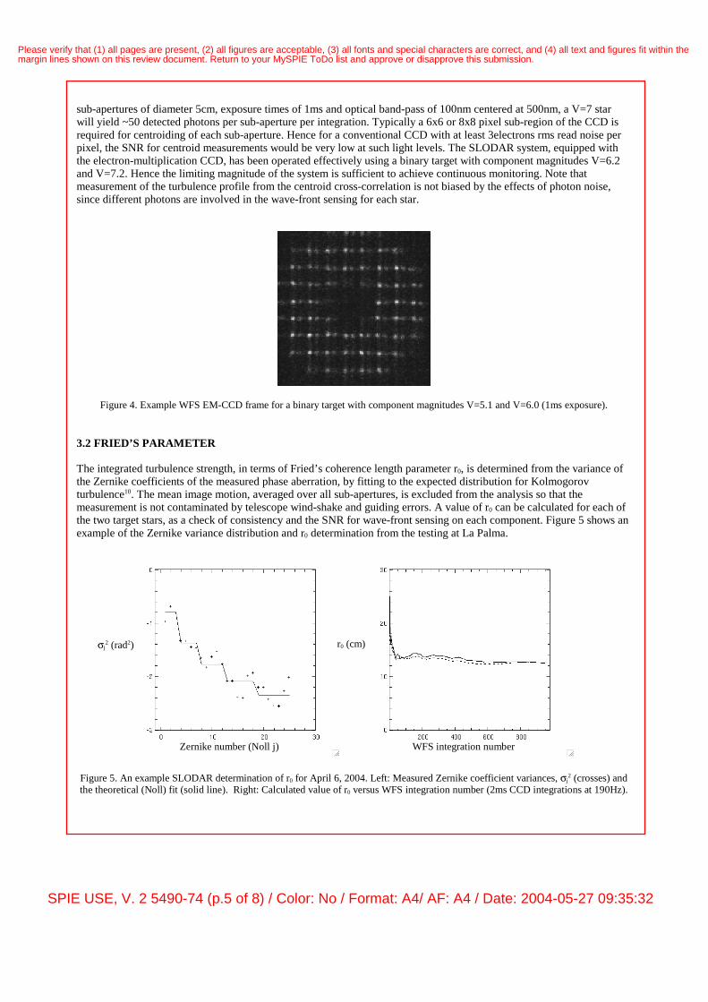
A custom-built portable enclosure has been provided for the system (Fig 3). The octagonal structure is constructed fromlightweight panels of anodized aluminium, providing good weather protection. The system can be operated with theenclosure in place and the roof open, or the structure can be completely removed to allow operation in the open air. Theenclosure can be disassembled into individual panels for transportation in standard transit cases. The total transit weightof the system, including the telescope and enclosure, is approx 500Kg in 7 cases.



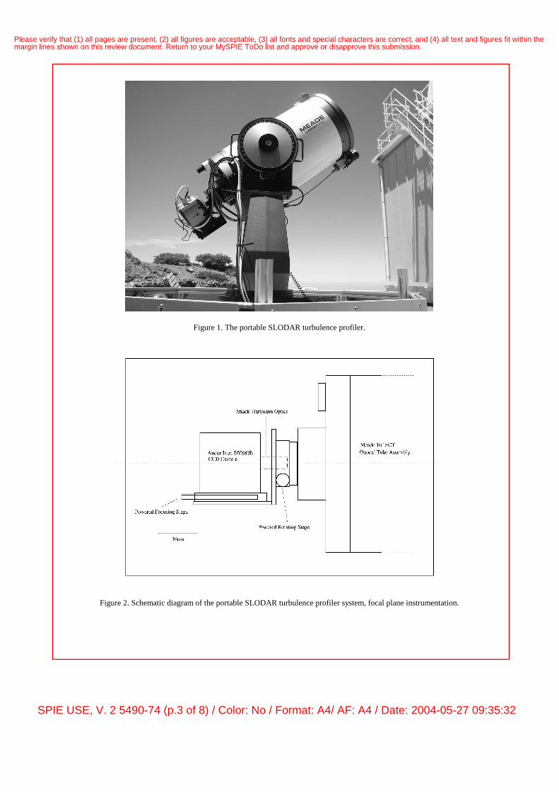
Figure 1. The portable SLODAR turbulence profiler.

Figure 2. Schematic diagram of the portable SLODAR turbulence profiler system, focal plane instrumentation.



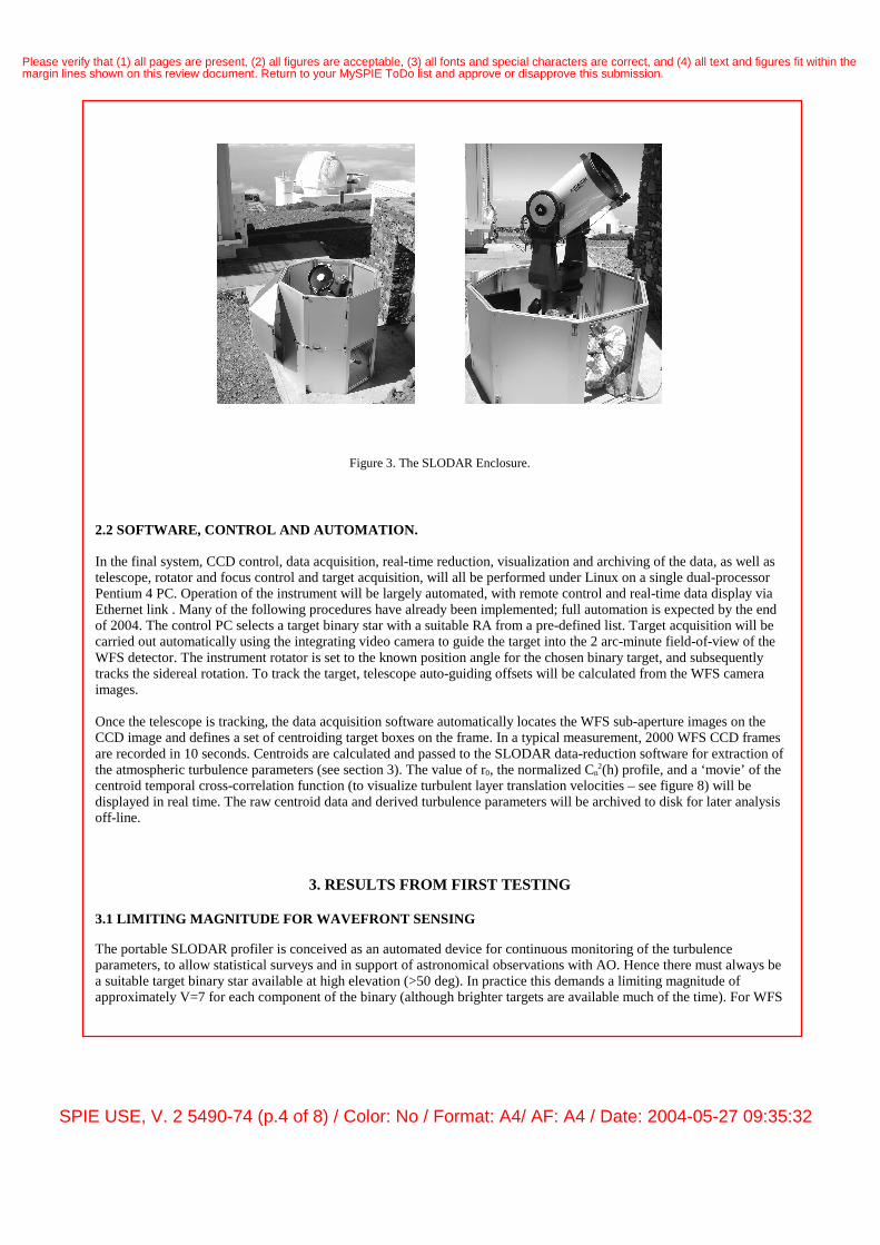
Figure 3. The SLODAR Enclosure.

2.2 SOFTWARE, CONTROL AND AUTOMATION.

In the final system, CCD control, data acquisition, real-time reduction, visualization and archiving of the data, as well astelescope, rotator and focus control and target acquisition, will all be performed under Linux on a single dual-processorPentium 4 PC. Operation of the instrument will be largely automated, with remote control and real-time data display viaEthernet link . Many of the following procedures have already been implemented; full automation is expected by the endof 2004. The control PC selects a target binary star with a suitable RA from a pre-defined list. Target acquisition will becarried out automatically using the integrating video camera to guide the target into the 2 arc-minute field-of-view of theWFS detector. The instrument rotator is set to the known position angle for the chosen binary target, and subsequentlytracks the sidereal rotation. To track the target, telescope auto-guiding offsets will be calculated from the WFS cameraimages.

Once the telescope is tracking, the data acquisition software automatically locates the WFS sub-aperture images on theCCD image and defines a set of centroiding target boxes on the frame. In a typical measurement, 2000 WFS CCD framesare recorded in 10 seconds. Centroids are calculated and passed to the SLODAR data-reduction software for extraction ofthe atmospheric turbulence parameters (see section 3). The value of r0, the normalized Cn

2(h) profile, and a ‘movie’ of thecentroid temporal cross-correlation function (to visualize turbulent layer translation velocities – see figure 8) will bedisplayed in real time. The raw centroid data and derived turbulence parameters will be archived to disk for later analysisoff-line.

3. RESULTS FROM FIRST TESTING

3.1 LIMITING MAGNITUDE FOR WAVEFRONT SENSING

The portable SLODAR profiler is conceived as an automated device for continuous monitoring of the turbulenceparameters, to allow statistical surveys and in support of astronomical observations with AO. Hence there must always bea suitable target binary star available at high elevation (>50 deg). In practice this demands a limiting magnitude ofapproximately V=7 for each component of the binary (although brighter targets are available much of the time). For WFS



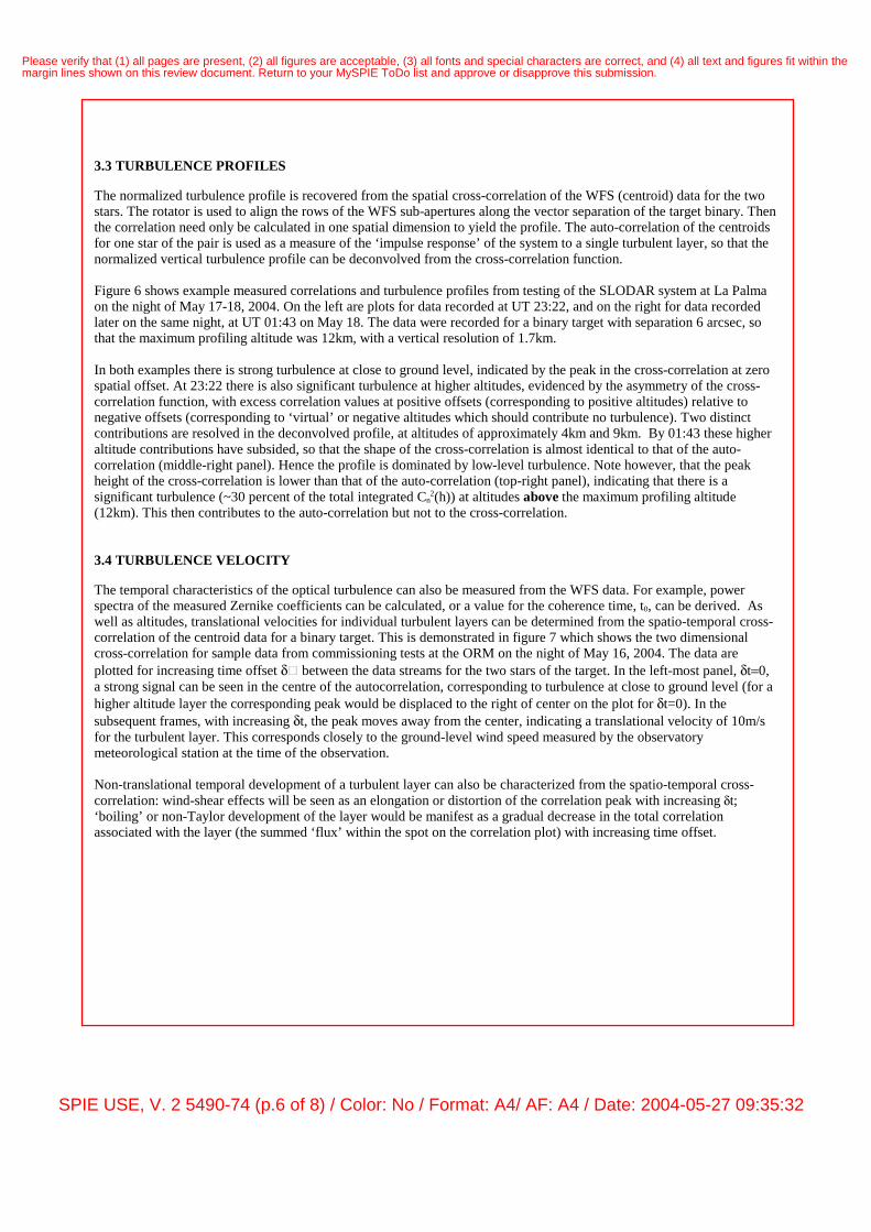
sub-apertures of diameter 5cm, exposure times of 1ms and optical band-pass of 100nm centered at 500nm, a V=7 starwill yield ~50 detected photons per sub-aperture per integration. Typically a 6x6 or 8x8 pixel sub-region of the CCD isrequired for centroiding of each sub-aperture. Hence for a conventional CCD with at least 3electrons rms read noise perpixel, the SNR for centroid measurements would be very low at such light levels. The SLODAR system, equipped withthe electron-multiplication CCD, has been operated effectively using a binary target with component magnitudes V=6.2and V=7.2. Hence the limiting magnitude of the system is sufficient to achieve continuous monitoring. Note thatmeasurement of the turbulence profile from the centroid cross-correlation is not biased by the effects of photon noise,since different photons are involved in the wave-front sensing for each star.

Figure 4. Example WFS EM-CCD frame for a binary target with component magnitudes V=5.1 and V=6.0 (1ms exposure).

3.2 FRIED’S PARAMETER

The integrated turbulence strength, in terms of Fried’s coherence length parameter r0, is determined from the variance ofthe Zernike coefficients of the measured phase aberration, by fitting to the expected distribution for Kolmogorovturbulence10. The mean image motion, averaged over all sub-apertures, is excluded from the analysis so that themeasurement is not contaminated by telescope wind-shake and guiding errors. A value of r0 can be calculated for each ofthe two target stars, as a check of consistency and the SNR for wave-front sensing on each component. Figure 5 shows anexample of the Zernike variance distribution and r0 determination from the testing at La Palma.

Figure 5. An example SLODAR determination of r0 for April 6, 2004. Left: Measured Zernike coefficient variances, σj2 (crosses) and

the theoretical (Noll) fit (solid line). Right: Calculated value of r0 versus WFS integration number (2ms CCD integrations at 190Hz).

Zernike number (Noll j)

σj2 (rad2) r0 (cm)

WFS integration number



3.3 TURBULENCE PROFILES

The normalized turbulence profile is recovered from the spatial cross-correlation of the WFS (centroid) data for the twostars. The rotator is used to align the rows of the WFS sub-apertures along the vector separation of the target binary. Thenthe correlation need only be calculated in one spatial dimension to yield the profile. The auto-correlation of the centroidsfor one star of the pair is used as a measure of the ‘impulse response’ of the system to a single turbulent layer, so that thenormalized vertical turbulence profile can be deconvolved from the cross-correlation function.

Figure 6 shows example measured correlations and turbulence profiles from testing of the SLODAR system at La Palmaon the night of May 17-18, 2004. On the left are plots for data recorded at UT 23:22, and on the right for data recordedlater on the same night, at UT 01:43 on May 18. The data were recorded for a binary target with separation 6 arcsec, sothat the maximum profiling altitude was 12km, with a vertical resolution of 1.7km.

In both examples there is strong turbulence at close to ground level, indicated by the peak in the cross-correlation at zerospatial offset. At 23:22 there is also significant turbulence at higher altitudes, evidenced by the asymmetry of the cross-correlation function, with excess correlation values at positive offsets (corresponding to positive altitudes) relative tonegative offsets (corresponding to ‘virtual’ or negative altitudes which should contribute no turbulence). Two distinctcontributions are resolved in the deconvolved profile, at altitudes of approximately 4km and 9km. By 01:43 these higheraltitude contributions have subsided, so that the shape of the cross-correlation is almost identical to that of the auto-correlation (middle-right panel). Hence the profile is dominated by low-level turbulence. Note however, that the peakheight of the cross-correlation is lower than that of the auto-correlation (top-right panel), indicating that there is asignificant turbulence (~30 percent of the total integrated Cn

2(h)) at altitudes above the maximum profiling altitude(12km). This then contributes to the auto-correlation but not to the cross-correlation.

3.4 TURBULENCE VELOCITY

The temporal characteristics of the optical turbulence can also be measured from the WFS data. For example, powerspectra of the measured Zernike coefficients can be calculated, or a value for the coherence time, t0, can be derived. Aswell as altitudes, translational velocities for individual turbulent layers can be determined from the spatio-temporal cross-correlation of the centroid data for a binary target. This is demonstrated in figure 7 which shows the two dimensionalcross-correlation for sample data from commissioning tests at the ORM on the night of May 16, 2004. The data areplotted for increasing time offset δ� between the data streams for the two stars of the target. In the left-most panel, δt=0,a strong signal can be seen in the centre of the autocorrelation, corresponding to turbulence at close to ground level (for ahigher altitude layer the corresponding peak would be displaced to the right of center on the plot for δt=0). In thesubsequent frames, with increasing δt, the peak moves away from the center, indicating a translational velocity of 10m/sfor the turbulent layer. This corresponds closely to the ground-level wind speed measured by the observatorymeteorological station at the time of the observation.

Non-translational temporal development of a turbulent layer can also be characterized from the spatio-temporal cross-correlation: wind-shear effects will be seen as an elongation or distortion of the correlation peak with increasing δt;‘boiling’ or non-Taylor development of the layer would be manifest as a gradual decrease in the total correlationassociated with the layer (the summed ‘flux’ within the spot on the correlation plot) with increasing time offset.



Figure 6. Example normalized cross-correlation functions and deconvolved turbulence profiles measured on May 17, 2004 (see text).Left: UT 23:22; Right: UT 01:43 (May 18). Top: Cross-correlation (solid line) and autocorrelation (broken line) functions normalizedto the peak value of the auto-correlation. Middle: The same cross-correlation and auto-correlation functions, each normalized to apeak value of 1 to allow comparison of the shape of the functions. Bottom: Deconvolved Cn

2(h) profiles, normalized to a peak value of1 (solid line ) and the cumulative profile (broken line). The integrated r0 values measured in each case were 11.0cm at 23:22 and11.9cm at 01:43.

Spatial Offset (sub-apertures) Spatial Offset (sub-apertures)

Spatial Offset (sub-apertures) Spatial Offset (sub-apertures)

Altitude (km) Altitude (km)



Figure 7. Example two dimensional centroid spatio-temporal cross-correlation function, with increasing temporal offset δt between thedata streams for the two stars of the target binary (see text). Left to right: δt = 0, increasing in 5ms steps to 20ms. The movement of thecorrelation peak is associated with a translational velocity of the low-altitude turbulence of 10m/s.

5. SUMMARY

A prototype portable system for profiling of the altitude and velocity of optical atmospheric turbulence is beingdeveloped, based on the SLODAR technique. Successful first field tests of the instrument have been carried out at LaPalma. Full automation of the system as a routine seeing and turbulence monitor is planned for the end of 2004.

ACKNOWLEDGEMENTS

The authors are grateful to the staff of the Isaac Newton group and the Instituto de Astrophysica de Canarias for theirassistance in facilitating field tests at the ORM, and for financial support from ESO and the UK PPARC (RWW). Wethank Tim Butterley, Tim Morris and Paul Clark for technical assistance.

REFERENCES

1. Vernin J., Munoz-Tunon, C., “Optical seeing at the La Palma Observatory”, A&A 284, 311, 1994.

2. Kluckers V.A., Wooder N.J., Nicholls M.J., Munro I., Dainty J.C., “Profiling of atmospheric turbulencestrength and velocity using a generalized SCIDAR technique”, A&AS 130, 141, 1998.

3. Avila R., Vernin J., Sanchez L.J., “Atmospheric turbulence and wind profile monitoring with generalizedSCIDAR”, A&A 369, 364, 2001.

4. Kornilov, V.K., et al., “MASS: a monitor of the vertical turbulence distribution”, proc. SPIE 4839, 837, 2003.

5. Wilson R.W., “SLODAR: Measuring optical turbulence altitude with a Shack--Hartmann wave-front sensor”,MNRAS 337, 103, 2002.

6. Wilson, R.W & Saunter, C.D., “Turbulence profiler and seeing monitor for laser guide star adaptive optics”,proc. SPIE 4839, 446, 2003.

7. Basden, A.G., Haniff, C.D. & Mackay, C.D., “Photon counting strategies with low light level CCDs”, MNRAS345, 985, 2003.

8. Marchetti, E., et al., “MAD: the ESO multi-conjugate adaptive optics demonstrator”, proc SPIE 4839, 317,2003.

9. Sarazin, M. & Roddier, F., “The ESO differential image motion monitor”, A&A 227, 294.

10. Noll, R., “Zernike polynomials and atmospheric turbulence”, JOSA 66, 207, 1976.



development of a portable slodar turbulence · pdf filedevelopment of a portable slodar...

Documents