DEVELOPMENT OF A SOFTWARE FOR SEISMIC DAMAGE ESTIMATION: CASE STUDIES

A THESIS SUBMITTED TO THE GRADUATE SCHOOL OF NATURAL AND APPLIED SCIENCES

OF MIDDLE EAST TECHNICAL UNIVERSITY

BY

SEZGİN KÜÇÜKÇOBAN

IN PARTIAL FULFILLMENT OF THE REQUIREMENTS FOR THE DEGREE OF

MASTER OF SCIENCE IN

CIVIL ENGINEERING

JULY 2004

Approval of the Graduate School of Natural and Applied Sciences

Prof. Dr. Canan Özgen Director

I certify that this thesis satisfies all the requirements as a thesis for the degree of Master of Science.

Prof. Dr. Erdal Çokça Head of Department

This is to certify that we have read this thesis and that in our opinion it is fully adequate, in scope and quality, as a thesis for the degree of Master of Science.

Asst. Prof. Dr. Ahmet Yakut Supervisor

Examining Committee Members Prof. Dr. Polat Gülkan (Chairman) (METU, CE)

Asst. Prof. Dr. Ahmet Yakut (METU, CE)

Prof. Dr. M. Semih Yücemen (METU, CE)

Asst. Prof. Dr. M. Altuğ Erberik (METU, CE)

M. S. Volkan Aydoğan (PROYA YAZILIM)

I hereby declare that all information in this document has been obtained and presented in accordance with academic rules and ethical conduct. I also declare that, as required by these rules and conduct, I have fully cited and referenced all material and results that are not original to this work. Name, Last name : Sezgin KÜÇÜKÇOBAN

Signature :

iii

ABSTRACT

DEVELOPMENT OF A SOFTWARE FOR SEISMIC

DAMAGE ESTIMATION: CASE STUDIES

Küçükçoban, Sezgin

M. S. Thesis, Department of Civil Engineering

Supervisor: Asst. Prof. Dr. Ahmet Yakut

July 2004, 147 pages

The occurrence of two recent major earthquakes, 17 August 1999 Mw = 7.4 Izmit

and 12 November 1999 Mw = 7.1 Düzce, in Turkey prompted seismologists and geologists

to conduct studies to predict magnitude and location of a potential earthquake that can

cause substantial damage in Istanbul. Many scenarios are available about the extent and

size of the earthquake. Moreover, studies have recommended rough estimates of risk areas

throughout the city to trigger responsible authorities to take precautions to reduce the

casualties and loss for the earthquake expected.

Most of these studies, however, adopt available procedure by modifying them for

the building stock peculiar to Turkey. The assumptions and modifications made are too

crude and thus are believed to introduce significant deviations from the actual case. To

minimize these errors and use specific damage functions and capacity curves that reflect

the practice in Turkey, a study was undertaken to predict damage pattern and distribution

in Istanbul for a scenario earthquake proposed by Japan International Cooperation Agency

iv

(JICA). The success of these studies strongly depends on the quality and validity of

building inventory and site property data.

Building damage functions and capacity curves developed from the studies

conducted in Middle East Technical University are used. A number of proper attenuation

relations are employed. The study focuses mainly on developing a software to carry out all

computations and present results. The results of this study reveal a more reliable picture of

the physical seismic damage distribution expected in Istanbul.

Keywords: Istanbul, earthquake, vulnerability analysis, risk assessment, damage curves,

seismic damage distribution, seismic risk analysis

v

ÖZ

SİSMİK HASAR TAHMİNİ İÇİN BİR BİLGİSAYAR PROGRAMI

GELİŞTİRİLMESİ: UYGULAMALAR

Küçükçoban, Sezgin

Yüksek Lisans Tezi, İnşaat Mühendisliği Bölümü

Tez Yöneticisi: Y. Doç. Dr. Ahmet Yakut

Temmuz 2004, 147 sayfa

Türkiye’de en son meydana gelen iki büyük deprem, 17 Ağustos 1999 Mw = 7.4

İzmit ve 12 Kasım 1999 Mw = 7.1 Düzce, deprembilim uzmanlarını ve jeologları

İstanbul’da büyük hasara sebep olabilecek olası bir depremin büyüklüğünü ve yerini

tahmin etmek için çalışmalar yapmaya yöneltmiştir. Depremin boyut ve büyüklüğü

hakkında birçok senaryo üretilmiştir. Üstelik, çalışmalar, sorumlu yetkilileri beklenen

deprem sonucundaki ölümleri ve kayıpları azaltacak önlemler almaları konusunda

harekete geçirmek için, şehrin her tarafında risk alanlarının kaba tahminlerini

önermektedir.

Fakat bu çalışmaların çoğu var olan prosedürleri Türkiye’ye özgü bina stoğu için

değiştirerek kullanılmaktadır. Yapılan kabuller ve değişiklikler çok üstünkörüdür ve bu

nedenle gerçek durumdan önemli derecede sapmalara yol açacağına inanılmaktadır. Bu

hataları azaltmak ve Türkiye’deki pratiği yansıtan özel hasar fonksiyonlarını ve kapasite

vi

eğrilerini kullanmak için, JICA tarafından önerilen bir senaryo deprem için İstanbul’daki

hasar modelini ve dağılımını tahmin etmek amacıyla bir çalışma ele alınmıştır. Çalışmanın

başarısı, büyük ölçüde arazi özelliği bilgilerine ve bina envanterinin kalitesine ve

geçerliliğine bağlıdır.

Orta Doğu Teknik Üniversitesi’nde yürütülen çalışmalardan elde edilen bina hasar

fonksiyonları ve kapasite eğrileri kullanılacak ve uygun azalım ilişkilerine yer verilecektir.

Bu çalışma, esas olarak, tüm hesaplamaları gerçekleştirecek ve sonuçları sunacak bir

program geliştirmeye odaklanacaktır. Çalışmanın sonuçları, İstanbul’da deprem nedeniyle

beklenen fiziksel hasar dağılımının daha güvenilir bir tablosunu açığa çıkaracaktır.

Anahtar Kelimeler: İstanbul, deprem, hasar görebilirlik analizi, risk değerlendirmesi, hasar

eğrileri, sismik hasar dağılımı, sismik tehlike analizi

vii

To My Family…

viii

ACKNOWLEDGMENTS

The author wishes to express his deepest gratitude to his supervisor Asst. Prof. Dr.

Ahmet Yakut for the insight, guidance, advices, criticisms, encouragements, and the

countless ideas that he has provided throughout this study.

My parents deserve endless appreciation for their confidence in me and for the

support, love and wisdom that they have provided throughout my life.

I am thankful to all my instructors that they have played a role in my education

and mental development.

My home mate Gökhan Özdemir, my office mate Serhat Bayılı, and my friend

Başar Özler are highly acknowledged for their invaluable friendship and assistance

throughout tense working periods.

Emre Akın, Emrah Erduran, İbrahim Erdem, Koray Sığırtmaç, Nazan Yılmaz

Öztürk, Musa Yılmaz, and Seval Pınarbaşı are among the precious people who have

always supported me with their beyond price friendship and love; they deserve the greatest

thanks.

The author also would like to thank all faculty members and structural mechanics

laboratory staff for the creative and dynamic working atmosphere that they have provided.

The research work presented in this study is supported in part by the Scientific

and Research Council of Turkey (TUBITAK) under grant: YMAU-ICTAG-I574 and by

NATO Scientific Affairs Division under grant: NATO SfP977231.

ix

TABLE OF CONTENTS

PLAGIARISM................................................................................................................. iii

ABSTRACT ......................................................................................................................iv

ÖZ……….. ........................................................................................................................vi

DEDICATION.............................................................................................................. viii

ACKNOWLEDGMENTS .............................................................................................. ix

TABLE OF CONTENTS.................................................................................................. x

LIST OF TABLES ......................................................................................................... xiii

LIST OF FIGURES......................................................................................................... xv

LIST OF SYMBOLS AND ABBREVIATIONS .................................................... xviii

CHAPTER

1. ...................................................................................................INTRODUCTION 1

1.1 BACKGROUND .................................................................................................... 1

1.2 LITERATURE SURVEY ......................................................................................... 2

1.2.1 ATC-13 Methodology................................................................................... 4

1.2.2 FEMA/NIBS Methodology ........................................................................... 5

1.2.3 JICA Study ................................................................................................... 7

1.2.4 KOERI Study.............................................................................................. 12

1.3 OBJECT AND SCOPE.......................................................................................... 16

2. THEORETICAL BACKGROUND ..................................................................... 17

2.1 GENERAL .......................................................................................................... 17

2.2 DISTANCE TYPE DEFINITIONS .......................................................................... 18

2.2.1 Linear Distance.......................................................................................... 19

x

2.2.2 Great Circle Distance ................................................................................ 20

2.2.3 Shortest Distance of a Point to a 3D Line Segment ................................... 21

2.3 ATTENUATION RELATIONSHIPS........................................................................ 24

2.3.1 Abrahamson and Silva [20] ....................................................................... 24

2.3.2 Boore et al. [12]......................................................................................... 27

2.3.3 Gülkan and Kalkan [21] ............................................................................ 27

2.3.4 Sadigh et al. [16] ....................................................................................... 30

2.3.5 Comparison of Attenuation Relationships ................................................. 33

2.4 COMPUTATION OF DISPLACEMENT DEMAND .................................................. 43

2.4.1 Capacity Spectrum Method (ATC-40 Procedure B) .................................. 43

2.4.2 Displacement Coefficient Method (FEMA-356) ........................................ 50

2.4.3 Constant Ductility Procedure (Chopra and Goel)..................................... 52

3. STRUCTURE OF THE SEISMIC RISK ANALYSIS SOFTWARE............... 55

3.1 INTRODUCTION ................................................................................................. 55

3.2 SOFTWARE COMPONENTS................................................................................. 55

3.2.1 Input Components ...................................................................................... 58

3.2.1.1 Building Inventory Data ...................................................................... 58

3.2.1.2 Capacity Curve Data............................................................................ 61

3.2.1.3 Scenario Earthquake Data ................................................................... 62

3.2.1.4 Attenuation Relationship Data ............................................................ 65

3.2.1.5 Analysis Method Data ......................................................................... 65

3.2.2 Calculation Components............................................................................ 67

3.2.2.1 Demand Calculation ............................................................................ 67

3.2.2.2 Performance Calculation ..................................................................... 68

3.2.2.3 Damage Estimation ............................................................................. 69

3.2.3 Output Components ................................................................................... 71

3.2.3.1 Screen Display..................................................................................... 71

3.2.3.2 Report Generation ............................................................................... 72

3.2.3.3 Exporting Results as Database File ..................................................... 73

xi

..................................................................................4. VERIFICATION OF SRAS 74

4.1 INTRODUCTION ................................................................................................. 74

4.2 INPUT PARAMETERS ......................................................................................... 75

4.3 DAMAGE ESTIMATION METHODOLOGY ........................................................... 77

4.4 RESULTS ........................................................................................................... 78

4.5 DISCUSSION OF RESULTS.................................................................................. 78

..................................................................................5. CASE STUDY: ISTANBUL 80

5.1 INTRODUCTION ................................................................................................. 80

5.2 DAMAGE ESTIMATION FOR ISTANBUL ............................................................. 81

5.2.1 JICA-Check ................................................................................................ 83

5.2.2 JICA-New................................................................................................... 85

5.2.3 IMM New ................................................................................................... 86

5.3 DISCUSSION OF RESULTS.................................................................................. 88

.........................................6. CONCLUSIONS AND RECOMMENDATIONS 101

6.1 SUMMARY........................................................................................................101

6.2 CONCLUSIONS..................................................................................................101

6.3 RECOMMENDATIONS FOR FUTURE STUDY ......................................................102

REFERENCES ............................................................................................................... 104

APPENDICES

A. SRAS MANUAL ................................................................................................. 108

B. CASE STUDY: ADAPAZARI ........................................................................... 129

C. CASE STUDY: ISTANBUL............................................................................... 136

xii

LIST OF TABLES

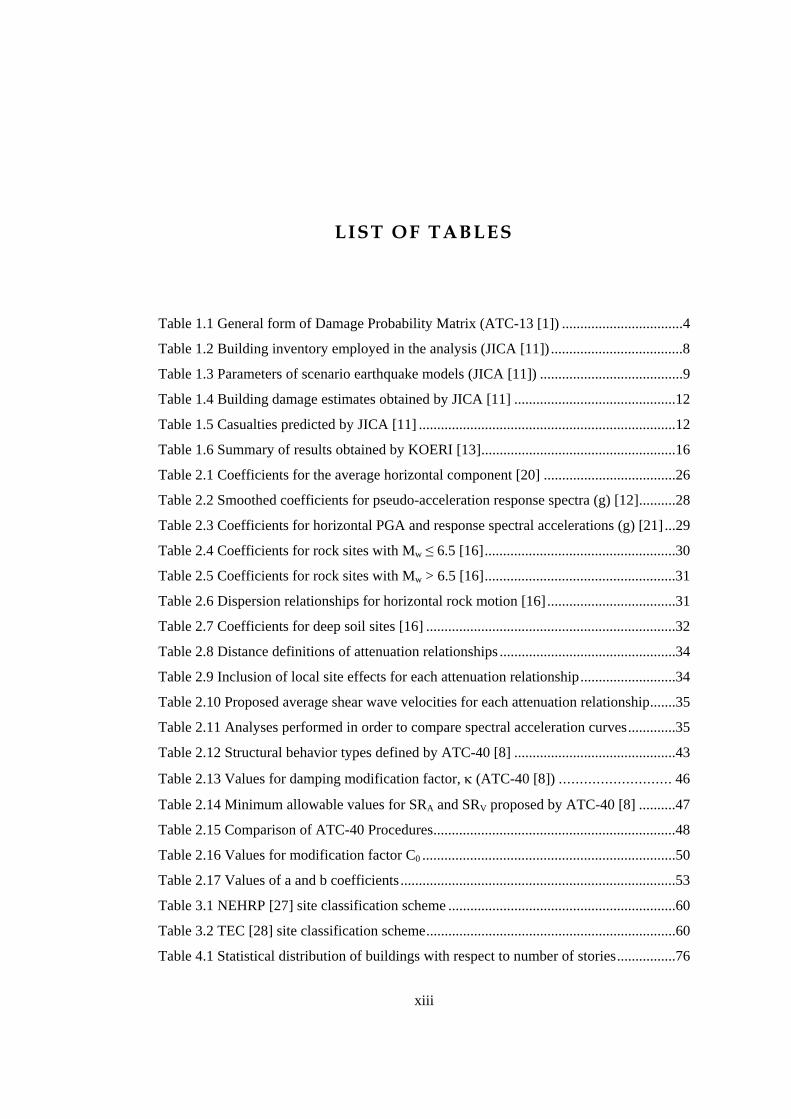
Table 1.1 General form of Damage Probability Matrix (ATC-13 [1]) .................................4

Table 1.2 Building inventory employed in the analysis (JICA [11]) ....................................8

Table 1.3 Parameters of scenario earthquake models (JICA [11]) .......................................9

Table 1.4 Building damage estimates obtained by JICA [11] ............................................12

Table 1.5 Casualties predicted by JICA [11] ......................................................................12

Table 1.6 Summary of results obtained by KOERI [13].....................................................16

Table 2.1 Coefficients for the average horizontal component [20] ....................................26

Table 2.2 Smoothed coefficients for pseudo-acceleration response spectra (g) [12]..........28

Table 2.3 Coefficients for horizontal PGA and response spectral accelerations (g) [21] ...29

Table 2.4 Coefficients for rock sites with Mw ≤ 6.5 [16]....................................................30

Table 2.5 Coefficients for rock sites with Mw > 6.5 [16]....................................................31

Table 2.6 Dispersion relationships for horizontal rock motion [16] ...................................31

Table 2.7 Coefficients for deep soil sites [16] ....................................................................32

Table 2.8 Distance definitions of attenuation relationships ................................................34

Table 2.9 Inclusion of local site effects for each attenuation relationship..........................34

Table 2.10 Proposed average shear wave velocities for each attenuation relationship.......35

Table 2.11 Analyses performed in order to compare spectral acceleration curves.............35

Table 2.12 Structural behavior types defined by ATC-40 [8] ............................................43

Table 2.13 Values for damping modification factor, κ (ATC-40 [8]) ........................... 46

Table 2.14 Minimum allowable values for SRA and SRV proposed by ATC-40 [8] ..........47

Table 2.15 Comparison of ATC-40 Procedures..................................................................48

Table 2.16 Values for modification factor C0 .....................................................................50

Table 2.17 Values of a and b coefficients...........................................................................53

Table 3.1 NEHRP [27] site classification scheme ..............................................................60

Table 3.2 TEC [28] site classification scheme....................................................................60

Table 4.1 Statistical distribution of buildings with respect to number of stories................76

xiii

LIST OF TABLES (CONTINUED)

Table 4.2 Vulnerability assessment criteria used in the analysis ........................................77

Table 5.1 Comparison of analyses performed for estimating damage in Istanbul..............81

Table 5.2 Selected maps and tables to be presented for each analysis ...............................82

Table 5.3 Building type statistics for JICA-Check .............................................................84

Table 5.4 Damage level limits defined for JICA-Check.....................................................85

Table 5.5 Building type statistics for JICA-New................................................................86

Table 5.6 Building type statistics for IMM-New................................................................87

Table 5.7 Summary of results obtained for JICA-Check....................................................97

Table 5.8 Summary of results obtained for JICA-New.......................................................98

Table 5.9 Summary of results obtained for IMM-New.......................................................99

Table 5.10 Summary of results obtained by JICA Study [11] ..........................................100

Table A.1 Interface differences between “Add … File” windows ...................................114

Table A.2 List of field types for building input file (Excel) .............................................126

Table A.3 List of field types for building input file (Access) ...........................................127

Table B.1 GDDA database damage statistics [30]............................................................129

Table B.2 Predicted damage for the GDDA dataset based on soft soil type and Gülkan and

Kalkan [21] attenuation relationship.................................................................................130

xiv

LIST OF FIGURES

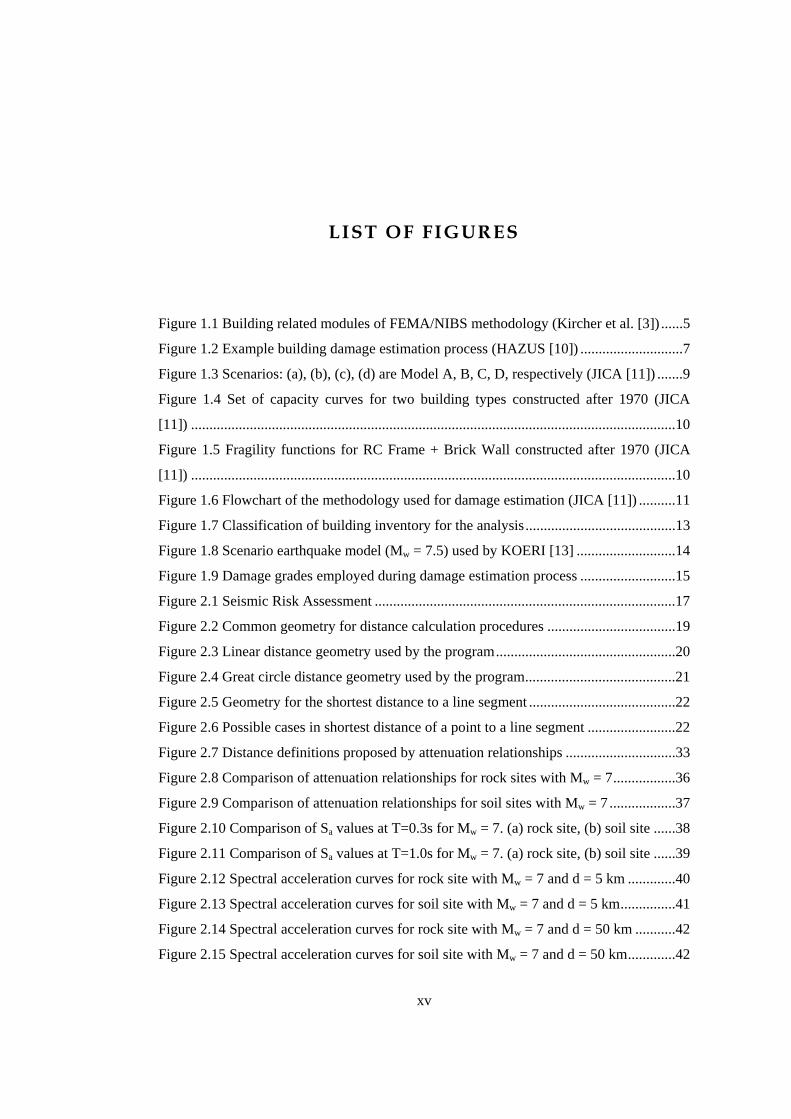
Figure 1.1 Building related modules of FEMA/NIBS methodology (Kircher et al. [3]) ......5

Figure 1.2 Example building damage estimation process (HAZUS [10]) ............................7

Figure 1.3 Scenarios: (a), (b), (c), (d) are Model A, B, C, D, respectively (JICA [11]) .......9

Figure 1.4 Set of capacity curves for two building types constructed after 1970 (JICA

[11]) ....................................................................................................................................10

Figure 1.5 Fragility functions for RC Frame + Brick Wall constructed after 1970 (JICA

[11]) ....................................................................................................................................10

Figure 1.6 Flowchart of the methodology used for damage estimation (JICA [11]) ..........11

Figure 1.7 Classification of building inventory for the analysis.........................................13

Figure 1.8 Scenario earthquake model (Mw = 7.5) used by KOERI [13] ...........................14

Figure 1.9 Damage grades employed during damage estimation process ..........................15

Figure 2.1 Seismic Risk Assessment ..................................................................................17

Figure 2.2 Common geometry for distance calculation procedures ...................................19

Figure 2.3 Linear distance geometry used by the program.................................................20

Figure 2.4 Great circle distance geometry used by the program.........................................21

Figure 2.5 Geometry for the shortest distance to a line segment ........................................22

Figure 2.6 Possible cases in shortest distance of a point to a line segment ........................22

Figure 2.7 Distance definitions proposed by attenuation relationships ..............................33

Figure 2.8 Comparison of attenuation relationships for rock sites with Mw = 7.................36

Figure 2.9 Comparison of attenuation relationships for soil sites with Mw = 7 ..................37

Figure 2.10 Comparison of Sa values at T=0.3s for Mw = 7. (a) rock site, (b) soil site ......38

Figure 2.11 Comparison of Sa values at T=1.0s for Mw = 7. (a) rock site, (b) soil site ......39

Figure 2.12 Spectral acceleration curves for rock site with Mw = 7 and d = 5 km .............40

Figure 2.13 Spectral acceleration curves for soil site with Mw = 7 and d = 5 km...............41

Figure 2.14 Spectral acceleration curves for rock site with Mw = 7 and d = 50 km ...........42

Figure 2.15 Spectral acceleration curves for soil site with Mw = 7 and d = 50 km.............42

xv

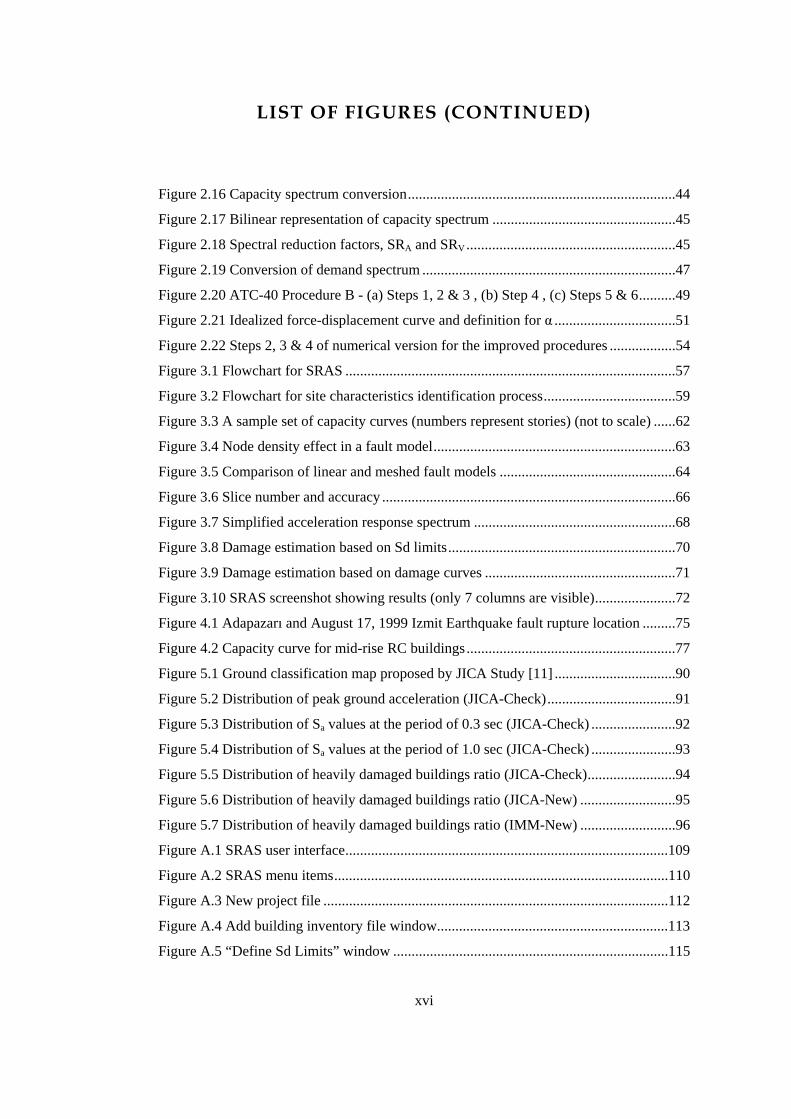
LIST OF FIGURES (CONTINUED)

Figure 2.16 Capacity spectrum conversion.........................................................................44

Figure 2.17 Bilinear representation of capacity spectrum ..................................................45

Figure 2.18 Spectral reduction factors, SRA and SRV.........................................................45

Figure 2.19 Conversion of demand spectrum .....................................................................47

Figure 2.20 ATC-40 Procedure B - (a) Steps 1, 2 & 3 , (b) Step 4 , (c) Steps 5 & 6..........49

Figure 2.21 Idealized force-displacement curve and definition for α .................................51

Figure 2.22 Steps 2, 3 & 4 of numerical version for the improved procedures ..................54

Figure 3.1 Flowchart for SRAS ..........................................................................................57

Figure 3.2 Flowchart for site characteristics identification process....................................59

Figure 3.3 A sample set of capacity curves (numbers represent stories) (not to scale) ......62

Figure 3.4 Node density effect in a fault model..................................................................63

Figure 3.5 Comparison of linear and meshed fault models ................................................64

Figure 3.6 Slice number and accuracy ................................................................................66

Figure 3.7 Simplified acceleration response spectrum .......................................................68

Figure 3.8 Damage estimation based on Sd limits..............................................................70

Figure 3.9 Damage estimation based on damage curves ....................................................71

Figure 3.10 SRAS screenshot showing results (only 7 columns are visible)......................72

Figure 4.1 Adapazarı and August 17, 1999 Izmit Earthquake fault rupture location .........75

Figure 4.2 Capacity curve for mid-rise RC buildings.........................................................77

Figure 5.1 Ground classification map proposed by JICA Study [11] .................................90

Figure 5.2 Distribution of peak ground acceleration (JICA-Check)...................................91

Figure 5.3 Distribution of Sa values at the period of 0.3 sec (JICA-Check) .......................92

Figure 5.4 Distribution of Sa values at the period of 1.0 sec (JICA-Check) .......................93

Figure 5.5 Distribution of heavily damaged buildings ratio (JICA-Check)........................94

Figure 5.6 Distribution of heavily damaged buildings ratio (JICA-New) ..........................95

Figure 5.7 Distribution of heavily damaged buildings ratio (IMM-New) ..........................96

Figure A.1 SRAS user interface........................................................................................109

Figure A.2 SRAS menu items...........................................................................................110

Figure A.3 New project file ..............................................................................................112

Figure A.4 Add building inventory file window...............................................................113

Figure A.5 “Define Sd Limits” window ...........................................................................115

xvi

LIST OF FIGURES (CONTINUED)

Figure A.6 Building type frame showing damage state labels..........................................116

Figure A.7 “Define Damage Curves” window .................................................................117

Figure A.8 The appearance of project file before starting the analysis ............................118

Figure A.9 Run window subsequent to completion of analysis........................................118

Figure A.10 “Results” frame after analysis has been completed ......................................119

Figure A.11 Tabular view of results .................................................................................120

Figure A.12 “User Details” tab in “Options” windows ....................................................121

Figure A.13 “Modification Factors” tab in “Options” menu ............................................122

Figure A.14 “Plotting Tool for Attenuation Relationships” window ...............................123

Figure B.1 PGA distribution obtained for different attenuation relationships..................131

Figure B.2 Distribution of Sa values at T = 0.3 s and 1.0 s for two attenuation relations.132

Figure B.3 Estimated percentage distribution of heavy damage/collapse using Gülkan and

Kalkan [21] (GDDA set)...................................................................................................133

Figure B.4 Estimated percentage distribution of moderate damage using Gülkan and

Kalkan [21] (GDDA set)...................................................................................................134

Figure B.5 Estimated damage for SU database based on soft soil using Boore et al.[12]135

Figure C.1 A sample group of capacity curves for RC buildings .....................................136

Figure C.2 Distribution of lightly damaged buildings ratio (JICA-Check) ......................137

Figure C.3 Distribution of moderately damaged buildings ratio (JICA-Check)...............138

Figure C.4 Distribution of lightly damaged buildings ratio (JICA-New) .........................139

Figure C.5 Distribution of moderately damaged buildings ratio (JICA-New) .................140

Figure C.6 New ground classification map proposed by this study..................................141

Figure C.7 Distribution of peak ground acceleration (IMM-New)...................................142

Figure C.8 Distribution of Sa values at the period of 0.3 sec (IMM-New) .......................143

Figure C.9 Distribution of Sa values at the period of 1.0 sec (IMM-New) .......................144

Figure C.10 Distribution of lightly damaged buildings ratio (IMM-New) .......................145

Figure C.11 Distribution of moderately damaged buildings ratio (IMM-New) ...............146

Figure C.12 Damage distribution obtained in IMM-New part (all-in-one) ......................147

xvii

LIST OF SYMBOLS AND ABBREVIATIONS

2D Two-dimensional

3D Three-dimensional

ACR American Red Cross

ADRS Acceleration-displacement response spectrum

api Spectral acceleration of trial performance point

ATC Applied Technology Council

ay Yield spectral acceleration

ave Average

BSSC Building Seismic Safety Council

CF Composite frame

Cm Effective mass factor

CSM Capacity spectrum method

D Distance

DC Damage curve

DF Damage factor

dpi Spectral displacement of trial performance point

dy Yield spectral displacement

EFC Earthquake Engineering Facility Classification

EN End node of segment

F Fault type

FEMA Federal Emergency Management Agency

g Acceleration of gravity

GDDA General Directorate of Disaster Affairs

GIS Geographical Information Systems

HW Hanging wall site dummy variable

ID Identification

xviii

LIST OF SYMBOLS AND ABBREVIATIONS

(CONTINUED)

IMM Istanbul Metropolitan Municipality

JICA Japan International Cooperation Agency

KIZILAY Turkish Red Crescent Society

KOERI Kandilli Observatory and Earthquake Research Institute

MDF Multi degree of freedom

MMI Modified Mercalli Intensity

MSK Medvedev-Sponheuer-Karnik

Mw Moment magnitude

NEHRP National Earthquake Hazard Reduction Program

NIBS National Institute of Building Sciences

PF1 Modal participation factor for the first natural mode

PGA Peak ground acceleration

PGV Peak ground velocity

pp performance point

R Ratio of elastic strength demand to the calculated yield strength coefficient

RC Reinforced concrete

RCF Reinforced concrete frame

rhypo Hypocentral distance

rjb Closest horizontal distance to the vertical projection of the rupture in km

rrup Closest distance to the rupture plane in km

Ry Yield reduction factor

S Dummy variable for the site class

Sa Spectral acceleration

Sd Spectral displacement

SDF Single degree of freedom

SDL Spectral displacement limit

SF Steel frame

SFC Social Function Classification

xix

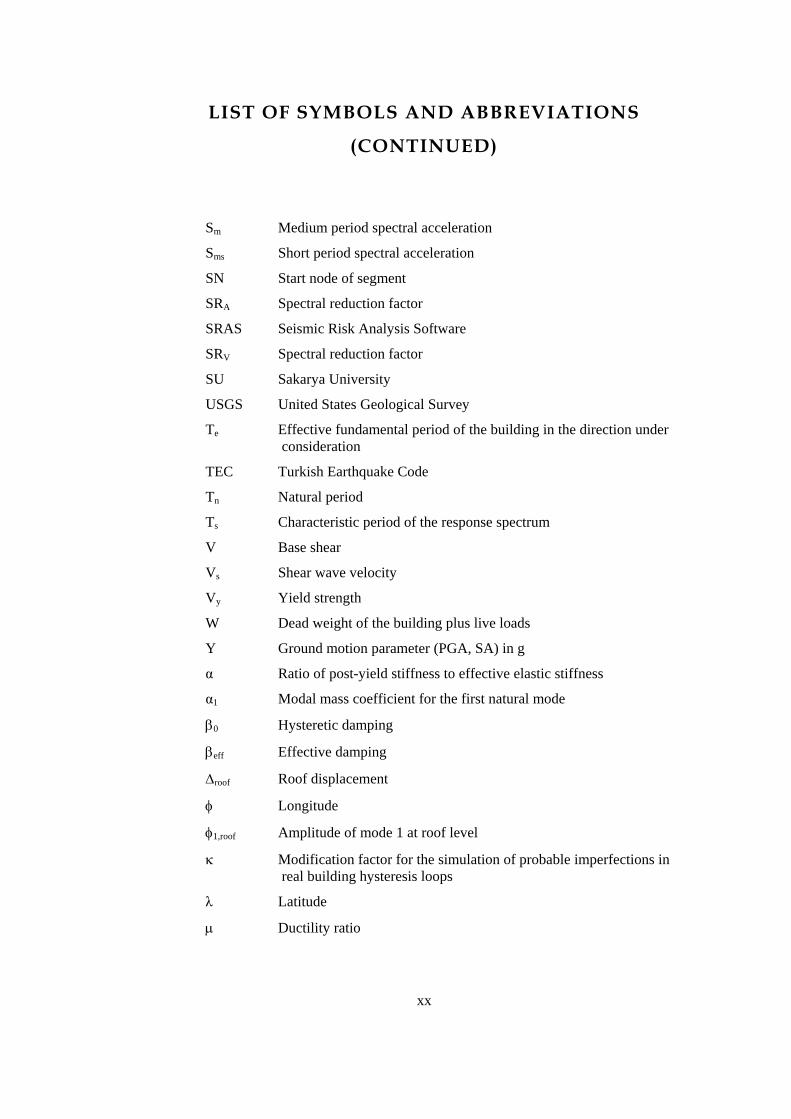
LIST OF SYMBOLS AND ABBREVIATIONS

(CONTINUED)

Sm Medium period spectral acceleration

Sms Short period spectral acceleration

SN Start node of segment

SRA Spectral reduction factor

SRAS Seismic Risk Analysis Software

SRV Spectral reduction factor

SU Sakarya University

USGS United States Geological Survey

Te Effective fundamental period of the building in the direction under consideration

TEC Turkish Earthquake Code

Tn Natural period

Ts Characteristic period of the response spectrum

V Base shear

Vs Shear wave velocity

Vy Yield strength

W Dead weight of the building plus live loads

Y Ground motion parameter (PGA, SA) in g

α Ratio of post-yield stiffness to effective elastic stiffness

α1 Modal mass coefficient for the first natural mode

β0 Hysteretic damping

βeff Effective damping

∆roof Roof displacement

φ Longitude

φ1,roof Amplitude of mode 1 at roof level

κ Modification factor for the simulation of probable imperfections in real building hysteresis loops

λ Latitude

µ Ductility ratio

xx

CHAPTER 1

INTRODUCTION

1.1 BACKGROUND

Turkey is one of the most seismically active countries in the world. This high

seismic nature results in an increase in damage potential as well as some other undesirable

consequences. Even if it seems impossible to estimate the outcome of future earthquakes

precisely, researchers have proposed several methodologies that yield rational predictions

for the adverse consequences. Some of these methodologies require detailed information

about the buildings such as structural and architectural configurations, material strengths

etc. whereas some others utilize only global information that can be easily obtained from a

street survey. Latter methodologies are generally branded as conventional regional

assessment procedures [30].

Conventional regional assessment procedures entail hazard assessment prior to

risk or damage evaluation. Hazard assessment can be carried out in two ways:

probabilistically and deterministically. Probabilistic method makes use of earthquake

source zones with their defined seismicity for a specific return period. The method can be

implemented with ease if a reliable earthquake database exists. It is performed to obtain

maximum ground motion parameters (e.g. peak ground acceleration (PGA), spectral

acceleration (Sa)) over the site with a certain probability of being exceeded in a given time

interval. On the other hand, deterministic method utilizes a scenario earthquake with its

defined geometry and magnitude. The method should be preferred only if a realistic and

highly probable scenario fault is readily available. After completion of hazard assessment,

regional vulnerability/risk assessment procedures provide rough estimates of high risk

areas and damage distribution pattern for the region.

1

Outcome of regional assessment procedures grants access to the development of

regional risk prevention/mitigation as well as disaster response planning management.

And also regional loss estimation and seismic microzonation studies make use of the

results generated by regional risk assessment procedures. Seismic loss estimation studies

are useful tools for state, regional and local governments in planning their emergency

management for future earthquakes.

Due to the recent devastating earthquakes in Turkey, administrative and public

authorities have realized the significance of disaster response planning prior to an

undesirable catastrophic experience. Public awareness has also forced municipalities to

implement seismic microzonation studies. Considering unprecedented increase in the

occurrence probability of a large magnitude earthquake in the proximity of Istanbul within

30 years, Istanbul Metropolitan Municipality (IMM) has initiated an extensive study for

risk prevention/mitigation and disaster response planning. Prediction of damage

distribution pattern in Istanbul was the essence of the project.

Regarding to the extremely large building database in Istanbul, the assessment

could only be performed in terms of 0.005˚ by 0.005˚ (approximately 500 m by 500 m)

cells where all buildings were lumped at the centers of the cells. Then, these cellular

damage predictions were merged and scaled to obtain sub-district level damage pattern

predictions. Conventional regional assessment procedures could not be fully employed for

the buildings individually since the process necessitates numerous calculations and time-

consuming database operations besides a reliable building inventory.

In this study, it is intended to develop seismic damage estimation software, which

is capable of handling buildings individually, and utilize the software in predicting

damage distribution in Istanbul. Thus, application of conventional regional assessment

procedures to different districts for several scenario earthquakes will be faster and simpler.

1.2 LITERATURE SURVEY

In many countries, there have been several seismic loss estimation studies in

district or sub-district level. Seismic loss estimation methodology consists of seismic

hazard, vulnerability and loss estimation studies. Seismic hazard analysis involves

compilation, preparation and analysis of earthquake catalog data, earthquake source

modeling, attenuation relationship and site properties. In vulnerability analysis, building

damage functions are developed to estimate building damage due to ground shaking. And

2

finally, the damage information obtained in vulnerability analysis part is converted to the

estimates of monetary loss. Among several loss estimation methodologies, the ones that

are widely accepted and implemented are discussed briefly in sections 1.2.1 and 1.2.2.

These widespread methodologies are known as ATC-13 (Applied Technology Council)

[1] and FEMA/NIBS (Federal Emergency Management Agency / National Institute of

Building Sciences) (Whitman et al. [2]) loss estimation methodologies. Since these

methodologies were developed to facilitate the estimation of earthquake induced losses for

a region, they demand intense and irritating database operations to extract regional

building inventory, possibly taking several months to a year to complete, prior to the

analysis phase. It was the shared shortcoming of regional loss estimation methodologies

and eliminated by the help of technology. Subsequent to the advances in geographical

information systems (GIS), software and computer technology, regional loss estimation

methodologies have become well-equipped. Nowadays, analyses are performed rapidly

and results are displayed graphically in a GIS environment. Thus, regional vulnerability

assessment has become handy for regional and local administrations while developing

strategies to reduce risks from future earthquakes and to be prepared for emergency

response and recovery.

Being one of the cultural, historical and economical centers in Turkey, Istanbul

has been the focus of such research projects. Vulnerability of the existing building

inventory and estimated damage distribution patterns have been investigated in a few

projects that are limited with the selected district boundaries. Besides these small scale

studies, two comprehensive studies were carried out for Istanbul Metropolitan Area by

different research teams, namely Japan International Cooperation Agency (JICA) and

Kandilli Observatory and Earthquake Research Institute (KOERI).

Since these studies cover all details of a well-organized seismic microzonation

practice, a summary which is mainly focusing on building damages will be presented in

sections 1.2.3 and 1.2.4 for the JICA Study [11] and KOERI Study [13], respectively. The

studies were examined in depth to extract what was taken as input, how it was processed

and what was computed as output. This data extraction is crucial for the determination of

the reliability of assessment as well as the validity of inherent assumptions. The

summaries are intentionally divided into three main parts: Input Data, Analysis and

Results. Each part presents brief and critical information about the study. They are tried to

be kept as concise as possible to facilitate rapid screening of what was done.

3

1.2.1 ATC-13 Methodology

The ATC-13 [1] was developed in 1985 and funded by the FEMA to develop

earthquake damage evaluation data for facilities in California. The data and damage/loss

estimation methodology are intended for estimating the economic consequences of a

major California earthquake on regional and national basis. The methodology presents

estimates of percent physical damage caused by ground shaking for the existing facilities

in California. Existing facilities have been classified in two ways:

1. by Earthquake Engineering Facility Classification (EEFC) (in terms of

structural system, type, size etc.)

2. by Social Function Classification (SFC) (in terms of their economic

function)

The EEFC contains 78 classes of structures, 40 of which are buildings and the rest

are other structure types. The SFC consists of 35 classes. The methodology is based on the

utilization of damage probability matrices. Estimates of percent physical damage caused

by ground shaking were developed through the estimates from more than 70 senior-level

specialists in earthquake engineering. These were expressed in terms of Damage Factor

(DF) versus Modified Mercalli Intensity (MMI) scale for all 78 facility classes. Damage

probability matrices were developed to estimate the expected dollar loss caused by ground

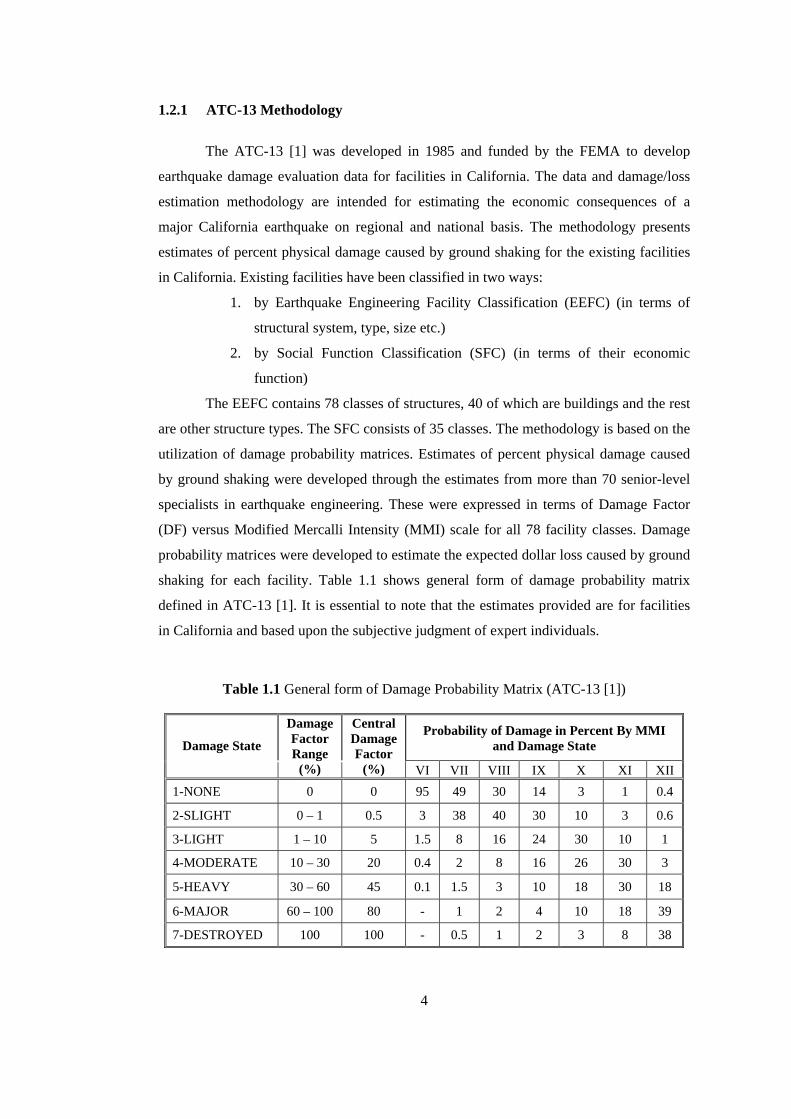
shaking for each facility. Table 1.1 shows general form of damage probability matrix

defined in ATC-13 [1]. It is essential to note that the estimates provided are for facilities

in California and based upon the subjective judgment of expert individuals.

Table 1.1 General form of Damage Probability Matrix (ATC-13 [1])

Probability of Damage in Percent By MMI and Damage State Damage State

Damage Factor Range

(%)

Central Damage Factor

(%) VI VII VIII IX X XI XII 1-NONE 0 0 95 49 30 14 3 1 0.4

2-SLIGHT 0 – 1 0.5 3 38 40 30 10 3 0.6

3-LIGHT 1 – 10 5 1.5 8 16 24 30 10 1

4-MODERATE 10 – 30 20 0.4 2 8 16 26 30 3

5-HEAVY 30 – 60 45 0.1 1.5 3 10 18 30 18

6-MAJOR 60 – 100 80 - 1 2 4 10 18 39

7-DESTROYED 100 100 - 0.5 1 2 3 8 38

4

1.2.2 FEMA/NIBS Methodology

Whitman et al. [2] summarized the development of a GIS based regional loss

estimation methodology for the United States funded by FEMA through NIBS. This

methodology was implemented in a software package (HAZUS) that operates through

MapInfo and ArcView, GIS applications. Methods for estimating building losses in the

FEMA/NIBS earthquake loss estimation methodology were described by Kircher et al.

[3]. The flow of the methodology between the modules related to building damage and

loss is shown Figure 1.1.

Figure 1.1 Building related modules of FEMA/NIBS methodology (Kircher et al. [3])

Thirty-six model building types are used by the methodology. These model

building types are based on the classification system of FEMA 178 [4]. The methodology

provides three approaches for defining an earthquake: the deterministic scenario event, the

scenario event based on probabilistic seismic hazard maps and the scenario event based on

user supplied ground shaking maps. Probabilistic spectral contour maps developed by the

United States Geological Survey (USGS) for the National Earthquake Hazard Reduction

Program (NEHRP) Provisions (Frankel et al. [5]) are employed. Attenuation equations

adopted by the USGS are utilized in HAZUS. Site specific response spectra are generated

by using ground motions at periods of 0.3 seconds and 1 second. Finally, ground motion

demands are modified by using site amplification factors developed by the Building

Seismic Safety Council for NEHRP-recommended building code standards (BSSC [6]).

5

In this methodology, two sets of functions or curves are used to estimate building

damage due to ground shaking:

1. Capacity curves that are used with damping modified demand spectra in order to

determine peak building response.

2. Fragility curves that describe the probability of reaching and exceeding different

state of damage at peak building response.

Building capacity curves strongly depend on the regional construction practice in

addition to regional seismicity and design code requirements. In regional vulnerability

analysis or loss estimation studies, typical capacity curves are needed for a group of

similar buildings rather than for a single building. In FEMA/NIBS methodology, the

capacity curves of various structural systems were developed based on the concepts

similar to those of FEMA 273 [7] and ATC-40 [8]. Each capacity curve is defined by two

control points: yield capacity and ultimate capacity. Kircher et al. [9] presented all

parameters, which are used to define yield and ultimate points, for some building types

and different code design levels in the FEMA/NIBS methodology.

Fragility curves provide estimates of the cumulative probabilities of being in, or

exceeding, slight, moderate, extensive and complete damage for the given level of ground

shaking or peak building response. FEMA/NIBS methodology uses fragility curves that

are functions of peak building response. Spectral displacement is the peak building

response used for calculating structural damage and nonstructural damage to drift-

sensitive components. Spectral acceleration is the peak building response used for

nonstructural damage to acceleration sensitive components.

FEMA/NIBS methodology employs the Capacity Spectrum Method (CSM) of

ATC-40 [8] to determine the peak building response in order to estimate losses from

future earthquakes. Peak building response is estimated from the intersection of the

capacity and demand curves. Probability of being or exceeding each damage state is

estimated using fragility curves and peak building response parameters (Sd for structural

components and drift-sensitive nonstructural components and Sa for acceleration-sensitive

nonstructural components) for structural and nonstructural components, separately. Figure

1.2 illustrates the building damage estimation process.

Finally, the damage information obtained in vulnerability analysis part is

converted to the estimates of monetary loss. Since details of loss estimation part are out of

scope of this study, they are not presented here.

6

Figure 1.2 Example building damage estimation process (HAZUS [10])

1.2.3 JICA Study

The study was performed by the team organized jointly by Pacific Consultants

International and OYO Corporation under the contract with JICA. It was a comprehensive

study on disaster prevention and mitigation basic plan for Istanbul including seismic

microzonation. The project was conducted in response to the request of the Government of

the Republic of Turkey. The study intended to integrate and develop seismic

microzonation studies carried out in Istanbul, recommend a city wide disaster prevention

and mitigation program and advise disaster prevention considerations to be integrated with

urban planning of Istanbul city.

7

1.2.3.1 Input Data

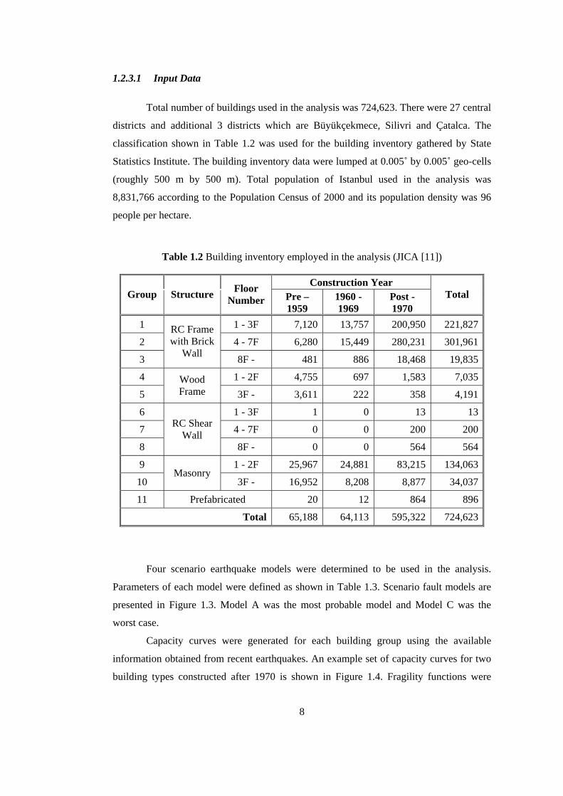
Total number of buildings used in the analysis was 724,623. There were 27 central

districts and additional 3 districts which are Büyükçekmece, Silivri and Çatalca. The

classification shown in Table 1.2 was used for the building inventory gathered by State

Statistics Institute. The building inventory data were lumped at 0.005˚ by 0.005˚ geo-cells

(roughly 500 m by 500 m). Total population of Istanbul used in the analysis was

8,831,766 according to the Population Census of 2000 and its population density was 96

people per hectare.

Table 1.2 Building inventory employed in the analysis (JICA [11])

Construction Year Group Structure Floor

Number Pre – 1959

1960 - 1969

Post - 1970

Total

1 1 - 3F 7,120 13,757 200,950 221,827

2 4 - 7F 6,280 15,449 280,231 301,961

3

RC Frame with Brick

Wall 8F - 481 886 18,468 19,835

4 1 - 2F 4,755 697 1,583 7,035

5 Wood Frame 3F - 3,611 222 358 4,191

6 1 - 3F 1 0 13 13

7 4 - 7F 0 0 200 200

8

RC Shear Wall

8F - 0 0 564 564

9 1 - 2F 25,967 24,881 83,215 134,063

10 Masonry

3F - 16,952 8,208 8,877 34,037

11 Prefabricated 20 12 864 896

Total 65,188 64,113 595,322 724,623

Four scenario earthquake models were determined to be used in the analysis.

Parameters of each model were defined as shown in Table 1.3. Scenario fault models are

presented in Figure 1.3. Model A was the most probable model and Model C was the

worst case.

Capacity curves were generated for each building group using the available

information obtained from recent earthquakes. An example set of capacity curves for two

building types constructed after 1970 is shown in Figure 1.4. Fragility functions were

8

utilized to determine damage ratios. These damage ratios were used while computing the

number of damaged buildings. Examples of these fragility functions for one building type

constructed after 1970 are presented in Figure 1.5.

Table 1.3 Parameters of scenario earthquake models (JICA [11])

Model A Model B Model C Model D

Length (km) 119 108 174 37

Moment magnitude (Mw) 7.5 7.4 7.7 6.9

Dip angle (Degree) 90 90 90 90

Depth of upper edge (km) 0 0 0 0

Type Strike-slip

Strike-slip

Strike-slip

Normal fault

Figure 1.3 Scenarios: (a), (b), (c), (d) are Model A, B, C, D, respectively (JICA [11])

9

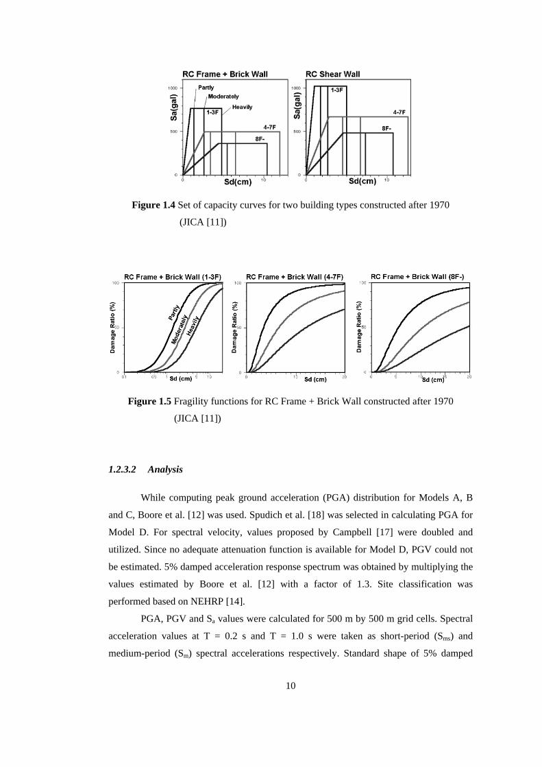
Figure 1.4 Set of capacity curves for two building types constructed after 1970

(JICA [11])

Figure 1.5 Fragility functions for RC Frame + Brick Wall constructed after 1970

(JICA [11])

1.2.3.2 Analysis

While computing peak ground acceleration (PGA) distribution for Models A, B

and C, Boore et al. [12] was used. Spudich et al. [18] was selected in calculating PGA for

Model D. For spectral velocity, values proposed by Campbell [17] were doubled and

utilized. Since no adequate attenuation function is available for Model D, PGV could not

be estimated. 5% damped acceleration response spectrum was obtained by multiplying the

values estimated by Boore et al. [12] with a factor of 1.3. Site classification was

performed based on NEHRP [14].

PGA, PGV and Sa values were calculated for 500 m by 500 m grid cells. Spectral

acceleration values at T = 0.2 s and T = 1.0 s were taken as short-period (Sms) and

medium-period (Sm) spectral accelerations respectively. Standard shape of 5% damped

10

response spectrum provided in NEHRP [14] was approximated with Sms and Sm. And also

“Average Horizontal Spectral Amplification” factors specified in NEHRP [14] were

utilized to modify the horizontal ground motions with respect to a nearby rock site

obtained by using Boore et al. [12].

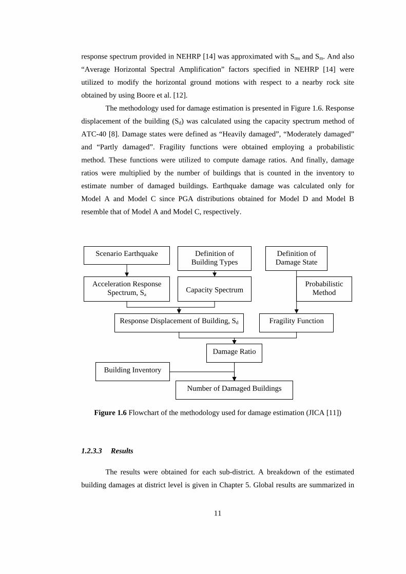
The methodology used for damage estimation is presented in Figure 1.6. Response

displacement of the building (Sd) was calculated using the capacity spectrum method of

ATC-40 [8]. Damage states were defined as “Heavily damaged”, “Moderately damaged”

and “Partly damaged”. Fragility functions were obtained employing a probabilistic

method. These functions were utilized to compute damage ratios. And finally, damage

ratios were multiplied by the number of buildings that is counted in the inventory to

estimate number of damaged buildings. Earthquake damage was calculated only for

Model A and Model C since PGA distributions obtained for Model D and Model B

resemble that of Model A and Model C, respectively.

Definition of Building Types

Definition of Damage State

Scenario Earthquake

Acceleration Response Spectrum, Sa

Figure 1.6 Flowchart of the methodology used for damage estimation (JICA [11])

1.2.3.3 Results

The results were obtained for each sub-district. A breakdown of the estimated

building damages at district level is given in Chapter 5. Global results are summarized in

Capacity Spectrum

Response Displacement of Building, Sd

Probabilistic Method

Fragility Function

Damage Ratio

Building Inventory

Number of Damaged Buildings

11

Table1.4 and 1.5 for building damages and casualties, respectively. Other assessment

results obtained for roads, bridges, lifelines, major urban facilities, hazardous facilities and

port and harbors will not be presented here.

Table 1.4 Building damage estimates obtained by JICA [11]

Heavily Heavily + Moderately

Heavily + Moderately +

Partly Building 51,000 114,000 252,000

Model A Household 216,000 503,000 1,116,000

Building 59,000 128,000 300,000 Model C

Household 268,000 601,000 1,300,000

Table 1.5 Casualties predicted by JICA [11]

Deaths Severely Injured

Model A 73,000 (0.8%) 120,000 (1.4%) Model C 87,000 (1.0%) 135,000 (1.5%)

1.2.4 KOERI Study

The study was performed by Earthquake Engineering Department of Boğaziçi

University and KOERI. It was an extensive study to develop a sub-district level

earthquake risk assessment for Istanbul. The project was proposed and funded by

American Red Cross (ACR), in collaboration with Turkish Red Crescent Society

(KIZILAY), in order to develop a basis for disaster response planning.

The ultimate objective of the study was to develop a sub-district level

earthquake risk assessment for Istanbul. Since this is an extensive task and composed of

several intermediate steps, two primary objectives were defined to clarify the overall

process. These primary objectives are developing a risk model for Istanbul, which

includes hazard assessment for a deterministic scenario earthquake (Mw = 7.5) and

predicting building damage, casualties, damage to infrastructure and lifelines.

12

1.2.4.1 Input Data

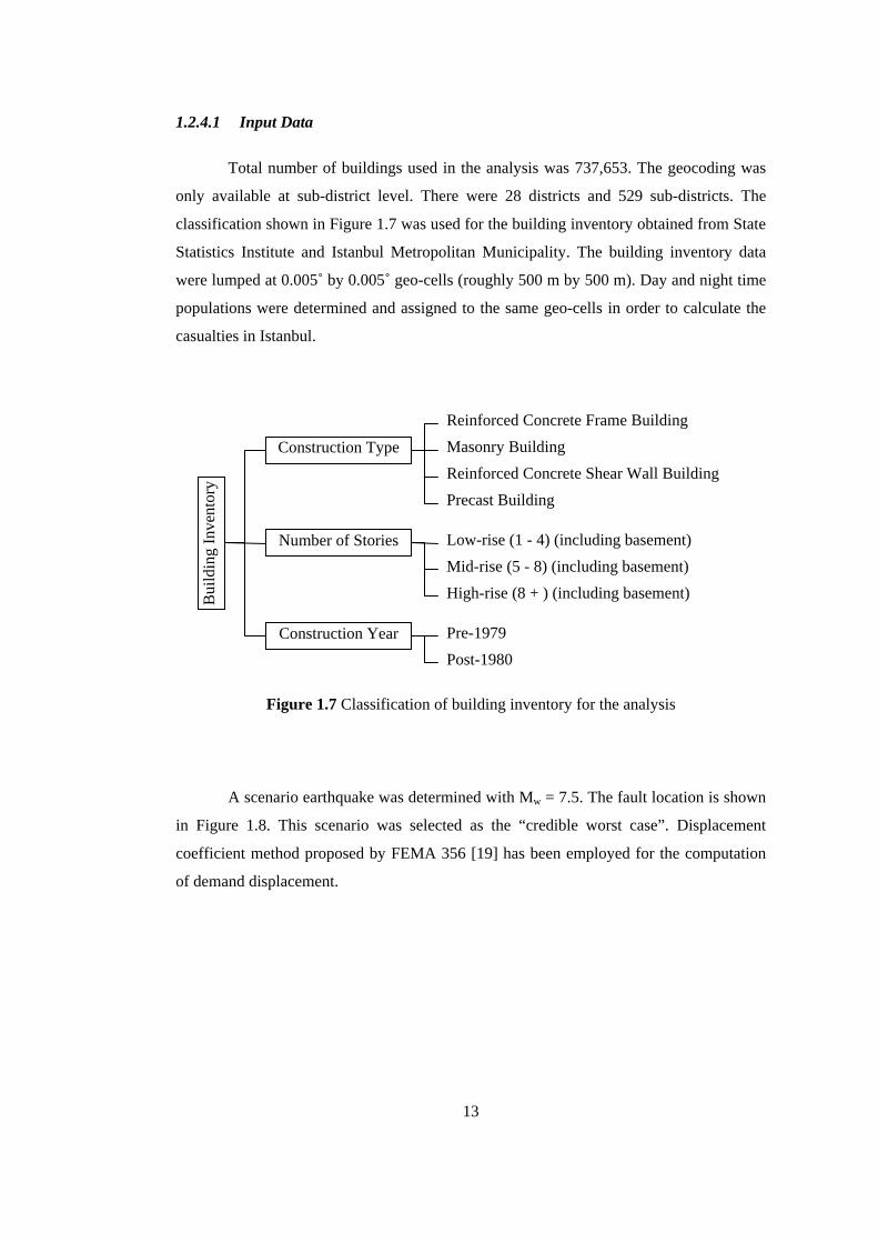
Total number of buildings used in the analysis was 737,653. The geocoding was

only available at sub-district level. There were 28 districts and 529 sub-districts. The

classification shown in Figure 1.7 was used for the building inventory obtained from State

Statistics Institute and Istanbul Metropolitan Municipality. The building inventory data

were lumped at 0.005˚ by 0.005˚ geo-cells (roughly 500 m by 500 m). Day and night time

populations were determined and assigned to the same geo-cells in order to calculate the

casualties in Istanbul.

Reinforced Concrete Frame Building

Figure 1.7 Classification of building inventory for the analysis

A scenario earthquake was determined with Mw = 7.5. The fault location is shown

in Figure 1.8. This scenario was selected as the “credible worst case”. Displacement

coefficient method proposed by FEMA 356 [19] has been employed for the computation

of demand displacement.

Bui

ldin

g In

vent

ory

Construction Type

Number of Stories

Construction Year

Masonry Building Reinforced Concrete Shear Wall Building Precast Building

Low-rise (1 - 4) (including basement) Mid-rise (5 - 8) (including basement) High-rise (8 + ) (including basement)

Pre-1979 Post-1980

13

Figure 1.8 Scenario earthquake model (Mw = 7.5) used by KOERI [13]

1.2.4.2 Analysis

While computing PGA distribution, the average of Boore et al. [12], Sadigh et al.

[16] and Campbell [17] relationships was used. For spectral acceleration values (Sa at T =

0.2 s and T = 1.0 s), the average of Boore et al. [12] and Sadigh et al. [16] was utilized.

Site classification was performed based on NEHRP [14]. Spectral acceleration values at

periods of 0.2 seconds and 1.0 second were taken as short-period (Sms) and medium-period

(Sm) spectral accelerations respectively. Standard shape of 5% damped response spectrum

provided in NEHRP [14] was approximated with Sms and Sm. And also “Average

Horizontal Spectral Amplification” factors specified in NEHRP [14] were utilized to

modify the horizontal ground motions with respect to a nearby rock site. Two separate

groups of ground motion parameters were assigned to geo-cells. The first group was site

dependent MSK intensities whereas the second was site dependent spectral accelerations

at T = 0.2 s and T = 1.0 s. The maximum value of the parameter relating to the cell was

assigned to that cell in order to be conservative.

The study employed two different methods for loss and damage estimation. First

method is based on spectral displacement. It takes spectral accelerations, capacity curves

for each building type and spectral displacement based vulnerabilities in order to compute

building damage ratios for each type of building. On the other hand, the second method is

based on MSK intensity. It takes seismic intensities and intensity based vulnerabilities

while calculating building damage ratios for each building type. These damage ratios were

used to estimate number of damaged buildings. And then direct economic losses and

casualties were computed. Casualties were calculated for four injury severity levels as

defined in HAZUS [15]. Damage grades for both methods are shown in Figure 1.9.

14

Figure 1.9 Damage grades employed during damage estimation process

Spectral displacement demand is estimated by using displacement coefficient

method of FEMA-356 [19]. Building capacities were tried to be approximated by

engineering judgment. The approximations made in HAZUS [15] were used directly or

modified to comprise site conditions. The vulnerability functions are based on the review

of existing models and the expert opinion in ATC-13 [1] supplemented by an expert

technical advisory group.

1.2.4.3 Results

The results were obtained in terms of geo-cells, sub-districts and districts. Global

results are summarized in Table 1.6 for building damages, number of casualties and

shelter needs. District level damage estimations are discussed in Chapter 5. The monetary

losses in the range of USD 11,250 million were estimated. Other results obtained for

Transportation, Telecommunication, Power Transmission, Natural Gas Transmission and

Sanitary Water and Waste Water Transmission Systems will not be presented here.

Spectral displacement based fragility curves

Slight Moderate Extensive Complete

MSK Intensity based vulnerability curves

D1 - Slight D2 - Moderate D3 - Heavy D4 – Partial Destruction D5 - Collapse

15

Table 1.6 Summary of results obtained by KOERI [13]

Damage Number

Collapse (D4+D5) 40,268 Intensity Based Method

Heavy Damage (D3) 76,944 Complete (Collapse) 34,828 Extensive 67,395 Sd Based Method Moderate 195,097

Casualty Severity Number Death 40,268

Intensity Based Method Hospitalized Injury 120,804 Severity 1 109,288 Severity 2 54,137 Severity 3 27,840

Sd Based Method

Severity 4 27,840 Shelter Need Number Intensity Based Method Household 608,908 Sd Based Method Household 431,671

1.3 OBJECT AND SCOPE

Within the scope of this study, it is intended to:

1. develop a regional seismic damage prediction software

2. verify the reliability of the software by simulating the August 17, 1999

Izmit Earthquake and predicting the damage distribution in Adapazarı

3. utilize the software developed in order to predict damage distribution

pattern in Istanbul resulted from a scenario earthquake (Model A

proposed by JICA [11]) using two different databases.

16

CHAPTER 2

THEORETICAL BACKGROUND

2.1 GENERAL

Seismic risk assessment plays a crucial role in determining the undesirable

consequences of future earthquakes. There are two different methods that may be followed

while performing seismic risk or hazard assessments; deterministic and probabilistic

(Figure 2.1). Deterministic method utilizes specific earthquake scenarios (earthquake

magnitude and location are known or predicted) whereas probabilistic method considers

all earthquakes with their probabilities of occurrences.

SEISMIC RISK ASSESSMENT

Deterministic Approach Probabilistic Approach

Scenario earthquakes Source seismicity

Figure 2.1 Seismic Risk Assessment

Considering the randomness inherited in earthquakes, the probabilistic framework

seems to be more qualified in describing risk. But, it requires a probabilistic seismic

hazard analysis which can be done only if a reliable database of earthquakes occurred in or

around the region under consideration, is available.

17

Deterministic approach is easier and faster to implement, but it is deficient in

taking into account the uncertainties and randomness. This approach is straightforward. A

scenario earthquake is defined with its fault location and magnitude. Then, attenuation

relations come into picture and provide expected ground motion parameters at the site. It

is not necessary to have an earthquake database for the region as it is the case in

probabilistic approach.

Since deterministic approach requires comparatively less data, time and effort, it

is extensively used in regional seismic risk assessments. Even if it is faster to implement,

the process becomes cumbersome when the number of scenario earthquakes, attenuation

relations, analysis methods and buildings increases. For this reason, development of a

computer program seems to be inevitable.

While developing software, basically, there are three steps that should be

followed. First step is gathering and integrating the theory used in the program. Second

step is generating algorithms and writing program codes. The final step is debugging

process which requires running of the software for many examples and capturing the

errors.

This theoretical background section is a consequence of the second step. Program

makes use of well-known attenuation relationships and displacement demand computation

methods. Since each of these will be declared frequently while discussing components of

the software, it is better to present here the theoretical background that is required for fully

understanding of the software components. Section 2.2 gives key definitions for distance

types referred throughout the study. The attenuation relationships are discussed in section

2.3 whereas section 2.4 discusses methods for computation of displacement demand.

2.2 DISTANCE TYPE DEFINITIONS

The program uses latitudes and longitudes while generating fault rupture path and

locating buildings. All distance calculation functions are based on the geometry and

symbols shown in Figure 2.2. Both spherical and 3D Cartesian coordinates are utilized in

order to obtain better distance calculation procedures.

18

z

Figure 2.2 Common geometry for distance calculation procedures

East and North directions are taken as positive while West and South directions

are taken as negative. It should be verified that coordinates of fault rupture path and

building locations are in the same projection system. Otherwise, distance calculations may

lead to errors or wrong results.

There are three different distance types used while creating a general algorithm

for the shortest distance to the fault rupture. The algorithm will be better understood if one

becomes skilled at these distance definitions.

2.2.1 Linear Distance

The length of a line segment combining two points on a sphere is known as linear

distance. This is the shortest distance between two points. Figure 2.3 shows the geometry

defined and used by the program.

O

kz1

x y

East (+) West (-)

0o

Equator

North (+)

South (-)

ky1 kx1

φ

θ

P (φ, λ)

λ

90o

r

19

z

Linear

Figure 2.3 Linear distance geometry used by the program

Conversion should be performed from spherical coordinates (λ, φ) to 3D Cartesian

coordinates (x, y, z). This can be done using the following equation set.

cosθrzsinsinθrycossinθrx

⋅=⋅⋅=⋅⋅=

φφ

(2.1)

where λ, φ: latitude, longitude

θ = 90˚ - λ

After converting spherical coordinates to 3D Cartesian coordinates, following

equation yields linear distance between points A(x1, y1, z1) and B(x2, y2, z2).

Dlinear = 212

212

212 )()()( zzyyxx −+−+− (2.2)

where x, y, z and Dlinear are all in km.

2.2.2 Great Circle Distance

It is the shortest distance that can be traveled between any two points on the

surface of a sphere. Figure 2.4 shows great circle geometry.

Equator

B(x2 , y2 , z2)

A(x1 , y1 , z1)

O

y x

B(λ2 , φ2)

A(λ1 , φ1)

20

z

Figure 2.4 Great circle distance geometry used by the program

Great circle distance is equal to multiplication of radius by α in radians. The

necessary formulation is provided below.

[ ])cos(coscossinsincosα 1221211 φφλλλλ −⋅⋅+⋅= − (2.3)

αrD circlegreat ⋅= (2.4)

where λ, φ: latitude, longitude

α in radians, r and Dgreat circle in km)

2.2.3 Shortest Distance of a Point to a 3D Line Segment

A line segment consists of all points on a line that are between two endpoints Po

and P1. A point on the sphere, named as P, and a line segment form a plane that should be

used for shortest distance calculations. Figure 2.5 shows the geometry.

O

A(λ1 , φ1)

Equator

Great Circle

(φ2 - φ1)

α

B(λ2 , φ2)

r

r

y x

21

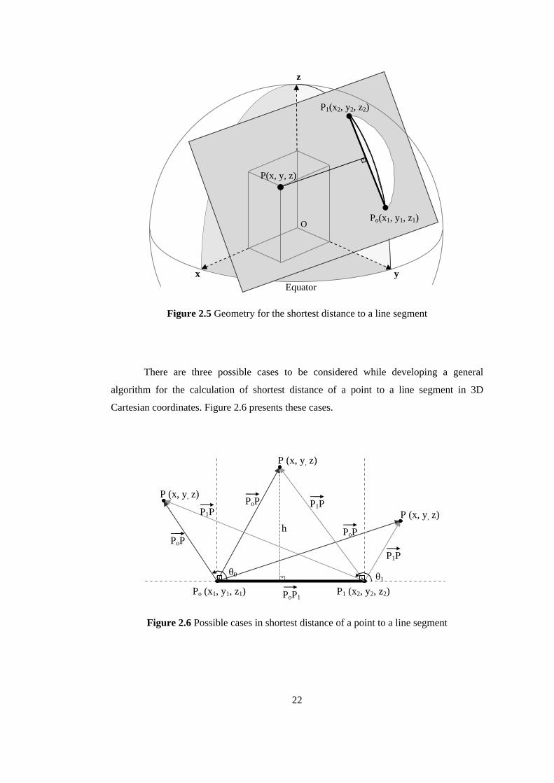
z

Figure 2.5 Geometry for the shortest distance to a line segment

There are three possible cases to be considered while developing a general

algorithm for the calculation of shortest distance of a point to a line segment in 3D

Cartesian coordinates. Figure 2.6 presents these cases.

Figure 2.6 Possible cases in shortest distance of a point to a line segment

Equator

O

y x

P1(x2, y2, z2)

.

P(x, y, z)

Po(x1, y1, z1)

P (x, y, z)

P (x, y, z) PoP P1P

Po (x1, y1, z1) P1 (x2, y2, z2)

P (x, y, z)

PoP

PoP1

P1P

PoP

. . .

P1P h

θ0 θ1

22

The general algorithm is provided below.

Case 1: Point P is to the left of line segment

Case 2: Point P is to the right of line segment

Case 3: Point P is within the rectangular region vertically traced by line segment

100 PP · PP result1=

If result1 < 0 Then (θ0 > 90°)

mindist = PPo Case 1

Exit Function End If

1010 PP · PP result2= If result2 < result1 Then (θ1 < 90°)

mindist = PP1 Case 2

Exit Function End If

u = ( 1oPP + PPo + PP1 )/2

area = 21

2o

21o )PP-(u)PP-(u)PP(uu ⋅⋅−⋅ Case 3

h = 10PP/area2 ⋅

mindist = h

In case 1, the sign of result1 indicates whether θ0 is greater or less than 90°. If

result1 is negative, this leads θ0 to be obtuse and shortest distance to be length of PPo .

In case 2, the condition [result2 < result1] must be satisfied. If result2 is smaller

than result1, this leads projection of PPo on 1oPP to be greater than 1oPP which in turn

guarantees that θ1 is less than 90°. As a result, shortest distance is the length of PP1 .

In case 3, u indicates semi-circumference of the triangle formed by three vectors.

After calculating area of the triangle, h which is the shortest distance is easily obtained.

23

2.3 ATTENUATION RELATIONSHIPS

Independent of seismic risk assessment methodology selection, the relationship

between ground motion, distance and magnitude has vital importance. Ground motion

prediction relationships can be expressed as equations that estimate ground motion as a

function of distance and magnitude as well as some other parameters such as type of

faulting, local site classification (condition), et cetera. In this study, four attenuation

relationships are used.

• Abrahamson and Silva [20]

• Boore et al. [12]

• Gülkan and Kalkan [21]

• Sadigh et al. [16]

Each attenuation relationship is summarized in the succeeding sections, mainly

focusing on the limitations and input parameters of each relationship. Databases, statistical

tools and numerical methods that are employed during development process of these

attenuation relationships are out of the scope of this study. Interested reader may easily

obtain detailed information from the reference papers.

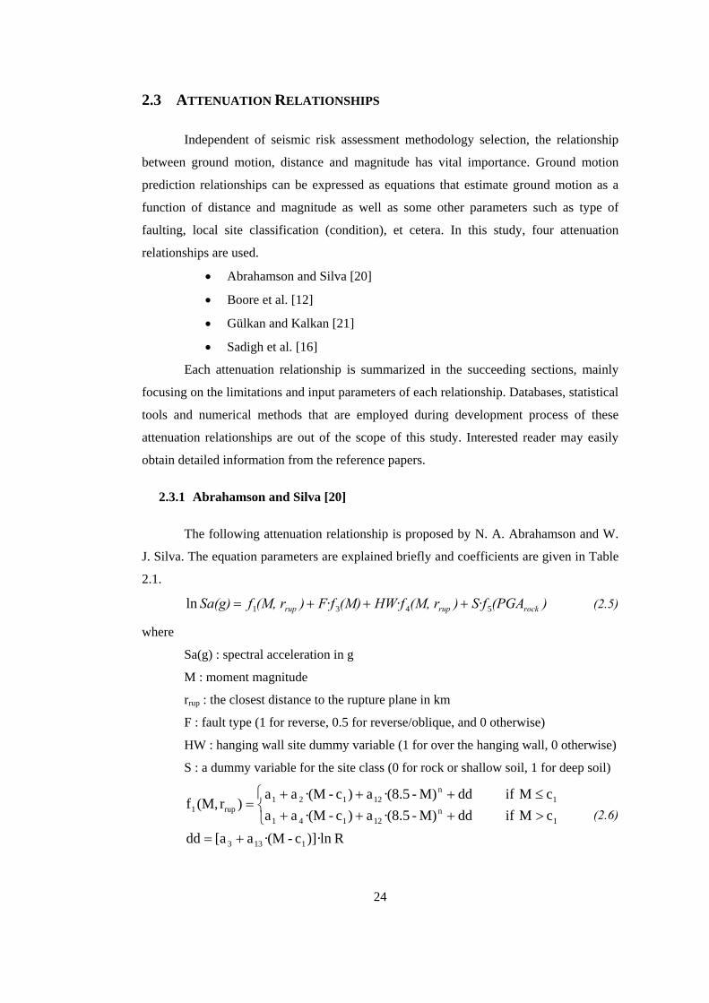
2.3.1 Abrahamson and Silva [20]

The following attenuation relationship is proposed by N. A. Abrahamson and W.

J. Silva. The equation parameters are explained briefly and coefficients are given in Table

2.1.

)(PGAS·f)(M, rHW·f(M)F·f)(M, rfSa(g) rockruprup 5431ln +++= (2.5)

where

Sa(g) : spectral acceleration in g

M : moment magnitude

rrup : the closest distance to the rupture plane in km

F : fault type (1 for reverse, 0.5 for reverse/oblique, and 0 otherwise)

HW : hanging wall site dummy variable (1 for over the hanging wall, 0 otherwise)

S : a dummy variable for the site class (0 for rock or shallow soil, 1 for deep soil)

R)]·ln c-·(Ma [addc M ifddM)-·(8.5a)c-·(Maac M ifddM)-·(8.5a)c-·(Ma a

)r(M,f

1133

1n

12141

1n

12121rup1

+=⎩⎨⎧

>+++≤+++

= (2.6)

24

24

2rup crR += (2.7)

⎪⎩

⎪⎨

⎧

≥<<−−+

≤=

16

11565

5

3

c Mfor ac M 5.8for 5.8))/(ca(aa

5.8 Mfor a(M)f (2.8)

)(r(M)·ff )r (M,f rupHWHWrup4 = (2.9)

⎪⎩

⎪⎨

⎧

≥<<−

≤=

6.5 Mfor 16.5 M 5.5for 5.5M

5.5 Mfor 0(M)fHW (2.10)

[ ]⎪⎪⎪

⎩

⎪⎪⎪

⎨

⎧

><<−−⋅<<<<−⋅

<

=

25rfor 024r18for 18)/7(r1a

18r8for a 8r4for 4)/4(ra

4rfor 0

)(rf

rup

ruprup9

rup9

ruprup9

rup

rupHW (2.11)

)c(PGA·ln aa )(PGAf 5rock1110rock5 ++= (2.12)

PGArock: the expected peak acceleration on rock in g (as predicted by the

attenuation relation with S=0)

This relationship uses a data set which is composed of 655 recordings from 58

earthquakes with Mw between 4.5 and 7.4 including 1994 Northridge earthquake. It is

appropriate for estimation of the average horizontal and vertical components for shallow

earthquakes in active tectonic regions. There is one limitation to be considered while using

this attenuation relationship. It should not be used to predict ground motions caused by

earthquakes having a moment magnitude less than 4.5 and greater than 7.4.

25

Table 2.1 Coefficients for the average horizontal component [20]

Period c4 a1 a3 a5 a6 a9 a10 a11 a12

0.01 5.6 1.64 -1.145 0.61 0.26 0.37 -0.417 -0.23 0

0.02 5.6 1.64 -1.145 0.61 0.26 0.37 -0.417 -0.23 0

0.03 5.6 1.69 -1.145 0.61 0.26 0.37 -0.47 -0.23 0.0143

0.04 5.6 1.78 -1.145 0.61 0.26 0.37 -0.555 -0.251 0.0245

0.05 5.6 1.87 -1.145 0.61 0.26 0.37 -0.62 -0.267 0.028

0.06 5.6 1.94 -1.145 0.61 0.26 0.37 -0.665 -0.28 0.03

0.075 5.58 2.037 -1.145 0.61 0.26 0.37 -0.628 -0.28 0.03

0.09 5.54 2.1 -1.145 0.61 0.26 0.37 -0.609 -0.28 0.03

0.1 5.5 2.16 -1.145 0.61 0.26 0.37 -0.598 -0.28 0.028

0.12 5.39 2.272 -1.145 0.61 0.26 0.37 -0.591 -0.28 0.018

0.15 5.27 2.407 -1.145 0.61 0.26 0.37 -0.577 -0.28 0.005

0.17 5.19 2.43 -1.135 0.61 0.26 0.37 -0.522 -0.265 -0.004

0.2 5.1 2.406 -1.115 0.61 0.26 0.37 -0.445 -0.245 -0.0138

0.24 4.97 2.293 -1.079 0.61 0.232 0.37 -0.35 -0.223 -0.0238

0.3 4.8 2.114 -1.035 0.61 0.198 0.37 -0.219 -0.195 -0.036

0.36 4.62 1.955 -1.0052 0.61 0.17 0.37 -0.123 -0.173 -0.046

0.4 4.52 1.86 -0.988 0.61 0.154 0.37 -0.065 -0.16 -0.0518

0.46 4.38 1.717 -0.9652 0.592 0.132 0.37 0.02 -0.136 -0.0594

0.5 4.3 1.615 -0.9515 0.581 0.119 0.37 0.085 -0.121 -0.0635

0.6 4.12 1.428 -0.9218 0.557 0.091 0.37 0.194 -0.089 -0.074

0.75 3.9 1.16 -0.8852 0.528 0.057 0.331 0.32 -0.05 -0.0862

0.85 3.81 1.02 -0.8648 0.512 0.038 0.309 0.37 -0.028 -0.0927

1 3.7 0.828 -0.8383 0.49 0.013 0.281 0.423 0 -0.102

1.5 3.55 0.26 -0.7721 0.438 -0.049 0.21 0.6 0.04 -0.12

2 3.5 -0.15 -0.725 0.4 -0.094 0.16 0.61 0.04 -0.14

3 3.5 -0.69 -0.725 0.4 -0.156 0.089 0.63 0.04 -0.1726

4 3.5 -1.13 -0.725 0.4 -0.2 0.039 0.64 0.04 -0.1956

5 3.5 -1.46 -0.725 0.4 -0.2 0 0.664 0.04 -0.215

Note: Other coefficients → a2 = 0.512, a4 = -0.144, a13 = 0.17, c1 = 6.4, c5 = 0.03, n=2

26

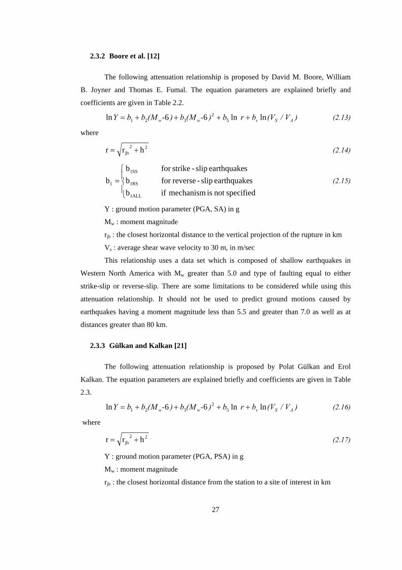
2.3.2 Boore et al. [12]

The following attenuation relationship is proposed by David M. Boore, William

B. Joyner and Thomas E. Fumal. The equation parameters are explained briefly and

coefficients are given in Table 2.2.

) / V(Vb rb)-(Mb)-(MbbY ASvww lnln66ln 52

321 ++++= (2.13)

where

22jb hrr += (2.14)

⎪⎩

⎪⎨

⎧=

specifiednot is mechanism ifbsearthquake slip-reversefor b

searthquake slip-strikefor bb

1ALL

1RS

1SS

1 (2.15)

Y : ground motion parameter (PGA, SA) in g

Mw : moment magnitude

rjb : the closest horizontal distance to the vertical projection of the rupture in km

Vs : average shear wave velocity to 30 m, in m/sec

This relationship uses a data set which is composed of shallow earthquakes in

Western North America with Mw greater than 5.0 and type of faulting equal to either

strike-slip or reverse-slip. There are some limitations to be considered while using this

attenuation relationship. It should not be used to predict ground motions caused by

earthquakes having a moment magnitude less than 5.5 and greater than 7.0 as well as at

distances greater than 80 km.

2.3.3 Gülkan and Kalkan [21]

The following attenuation relationship is proposed by Polat Gülkan and Erol

Kalkan. The equation parameters are explained briefly and coefficients are given in Table

2.3.

) / V(Vb rb)-(Mb)-(MbbY ASvww lnln66ln 52

321 ++++= (2.16)

where

22jb hrr += (2.17)

Y : ground motion parameter (PGA, PSA) in g

Mw : moment magnitude

rjb : the closest horizontal distance from the station to a site of interest in km

27

Table 2.2 Smoothed coefficients for pseudo-acceleration response spectra (g) [12]

Period b1SS b1RV b1ALL b2 b3 b5 bv VA h σln(Y)

0 -0.313 -0.117 -0.242 0.527 0 -0.778 -0.371 1396 5.57 0.5200.1 1.006 1.087 1.059 0.753 -0.226 -0.934 -0.212 1112 6.27 0.479

0.11 1.072 1.164 1.13 0.732 -0.23 -0.937 -0.211 1291 6.65 0.4810.12 1.109 1.215 1.174 0.721 -0.233 -0.939 -0.215 1452 6.91 0.4850.13 1.128 1.246 1.2 0.711 -0.233 -0.939 -0.221 1596 7.08 0.4860.14 1.135 1.261 1.208 0.707 -0.23 -0.938 -0.228 1718 7.18 0.4890.15 1.128 1.264 1.204 0.702 -0.228 -0.937 -0.238 1820 7.23 0.4920.16 1.112 1.257 1.192 0.702 -0.226 -0.935 -0.248 1910 7.24 0.4950.17 1.09 1.242 1.173 0.702 -0.221 -0.933 -0.258 1977 7.21 0.4970.18 1.063 1.222 1.151 0.705 -0.216 -0.93 -0.27 2037 7.16 0.4990.19 1.032 1.198 1.122 0.709 -0.212 -0.927 -0.281 2080 7.1 0.5010.2 0.999 1.17 1.089 0.711 -0.207 -0.924 -0.292 2118 7.02 0.502

0.22 0.925 1.104 1.019 0.721 -0.198 -0.918 -0.315 2158 6.83 0.5080.24 0.847 1.033 0.941 0.732 -0.189 -0.912 -0.338 2178 6.62 0.5110.26 0.764 0.958 0.861 0.744 -0.18 -0.906 -0.36 2173 6.39 0.5140.28 0.681 0.881 0.78 0.758 -0.168 -0.899 -0.381 2158 6.17 0.5180.3 0.598 0.803 0.7 0.769 -0.161 -0.893 -0.401 2133 5.94 0.522

0.32 0.518 0.725 0.619 0.783 -0.152 -0.888 -0.42 2104 5.72 0.5250.34 0.439 0.648 0.54 0.794 -0.143 -0.882 -0.438 2070 5.5 0.5300.36 0.361 0.57 0.462 0.806 -0.136 -0.877 -0.456 2032 5.3 0.5320.38 0.286 0.495 0.385 0.82 -0.127 -0.872 -0.472 1995 5.1 0.5360.4 0.212 0.423 0.311 0.831 -0.12 -0.867 -0.487 1954 4.91 0.538

0.42 0.14 0.352 0.239 0.84 -0.113 -0.862 -0.502 1919 4.74 0.5420.44 0.073 0.282 0.169 0.852 -0.108 -0.858 -0.516 1884 4.57 0.5450.46 0.005 0.217 0.102 0.863 -0.101 -0.854 -0.529 1849 4.41 0.5490.48 -0.058 0.151 0.036 0.873 -0.097 -0.85 -0.541 1816 4.26 0.5510.5 -0.122 0.087 -0.025 0.884 -0.09 -0.846 -0.553 1782 4.13 0.556

0.55 -0.268 -0.063 -0.176 0.907 -0.078 -0.837 -0.579 1710 3.82 0.5620.6 -0.401 -0.203 -0.314 0.928 -0.069 -0.83 -0.602 1644 3.57 0.569

0.65 -0.523 -0.331 -0.44 0.946 -0.06 -0.823 -0.622 1592 3.36 0.5750.7 -0.634 -0.452 -0.555 0.962 -0.053 -0.818 -0.639 1545 3.2 0.582

0.75 -0.737 -0.562 -0.661 0.979 -0.046 -0.813 -0.653 1507 3.07 0.5870.8 -0.829 -0.666 -0.76 0.992 -0.041 -0.809 -0.666 1476 2.98 0.593

0.85 -0.915 -0.761 -0.851 1.006 -0.037 -0.805 -0.676 1452 2.92 0.5980.9 -0.993 -0.848 -0.933 1.018 -0.035 -0.802 -0.685 1432 2.89 0.604

0.95 -1.066 -0.932 -1.01 1.027 -0.032 -0.8 -0.692 1416 2.88 0.6091 -1.133 -1.009 -1.08 1.036 -0.032 -0.798 -0.698 1406 2.9 0.613

1.1 -1.249 -1.145 -1.208 1.052 -0.03 -0.795 -0.706 1396 2.99 0.6221.2 -1.345 -1.265 -1.315 1.064 -0.032 -0.794 -0.71 1400 3.14 0.6291.3 -1.428 -1.37 -1.407 1.073 -0.035 -0.793 -0.711 1416 3.36 0.6371.4 -1.495 -1.46 -1.483 1.08 -0.039 -0.794 -0.709 1442 3.62 0.6431.5 -1.552 -1.538 -1.55 1.085 -0.044 -0.796 -0.704 1479 3.92 0.6491.6 -1.598 -1.608 -1.605 1.087 -0.051 -0.798 -0.697 1524 4.26 0.6541.7 -1.634 -1.668 -1.652 1.089 -0.058 -0.801 -0.689 1581 4.62 0.6601.8 -1.663 -1.718 -1.689 1.087 -0.067 -0.804 -0.679 1644 5.01 0.6641.9 -1.685 -1.763 -1.72 1.087 -0.074 -0.808 -0.667 1714 5.42 0.6692 -1.699 -1.801 -1.743 1.085 -0.085 -0.812 -0.655 1795 5.85 0.672

28

Table 2.3 Coefficients for horizontal PGA and response spectral accelerations (g) [21]

Period b1 b2 b3 b5 bv VA h σln(Y)

0 -0.682 0.253 0.036 -0.562 -0.297 1381 4.48 0.562 0.1 -0.139 0.2 -0.003 -0.553 -0.167 1063 3.76 0.621

0.11 0.031 0.235 -0.007 -0.573 -0.181 1413 3.89 0.618 0.12 0.123 0.228 -0.031 -0.586 -0.208 1501 4.72 0.615 0.13 0.138 0.216 -0.007 -0.59 -0.237 1591 5.46 0.634 0.14 0.1 0.186 0.014 -0.585 -0.249 1833 4.98 0.635 0.15 0.09 0.21 -0.013 -0.549 -0.196 1810 2.77 0.620 0.16 -0.128 0.214 0.007 -0.519 -0.224 2193 1.32 0.627 0.17 -0.107 0.187 0.037 -0.535 -0.243 2433 1.67 0.621 0.18 0.045 0.168 0.043 -0.556 -0.256 2041 2.44 0.599 0.19 0.053 0.18 0.063 -0.57 -0.288 2086 2.97 0.601 0.2 0.127 0.192 0.065 -0.597 -0.303 2238 3.48 0.611

0.22 -0.081 0.214 0.006 -0.532 -0.319 2198 1.98 0.584 0.24 -0.167 0.265 -0.035 -0.531 -0.382 2198 2.55 0.569 0.26 -0.129 0.345 -0.039 -0.552 -0.395 2160 3.45 0.549 0.28 0.14 0.428 -0.096 -0.616 -0.369 2179 4.95 0.530 0.3 0.296 0.471 -0.14 -0.642 -0.346 2149 6.11 0.540

0.32 0.454 0.476 -0.168 -0.653 -0.29 2144 7.38 0.555 0.34 0.422 0.471 -0.152 -0.651 -0.3 2083 8.3 0.562 0.36 0.554 0.509 -0.114 -0.692 -0.287 2043 9.18 0.563 0.38 0.254 0.499 -0.105 -0.645 -0.341 2009 9.92 0.562 0.4 0.231 0.497 -0.105 -0.647 -0.333 1968 9.92 0.604

0.42 0.12 0.518 -0.135 -0.612 -0.313 1905 9.09 0.634 0.44 0.035 0.544 -0.142 -0.583 -0.286 1899 9.25 0.627 0.46 -0.077 0.58 -0.147 -0.563 -0.285 1863 8.98 0.642 0.48 -0.154 0.611 -0.154 -0.552 -0.293 1801 8.96 0.653 0.5 -0.078 0.638 -0.161 -0.565 -0.259 1768 9.06 0.679

0.55 -0.169 0.707 -0.179 -0.539 -0.216 1724 8.29 0.710 0.6 -0.387 0.698 -0.187 -0.506 -0.259 1629 8.24 0.707

0.65 -0.583 0.689 -0.159 -0.5 -0.304 1607 7.64 0.736 0.7 -0.681 0.698 -0.143 -0.517 -0.36 1530 7.76 0.743

0.75 -0.717 0.73 -0.143 -0.516 -0.331 1492 7.12 0.740 0.8 -0.763 0.757 -0.113 -0.525 -0.302 1491 6.98 0.742

0.85 -0.778 0.81 -0.123 -0.529 -0.283 1438 6.57 0.758 0.9 -0.837 0.856 -0.13 -0.512 -0.252 1446 7.25 0.754

0.95 -0.957 0.87 -0.127 -0.472 -0.163 1384 7.24 0.752 1 -1.112 0.904 -0.169 -0.443 -0.2 1391 6.63 0.756

1.1 -1.459 0.898 -0.147 -0.414 -0.252 1380 6.21 0.792 1.2 -1.437 0.962 -0.156 -0.463 -0.267 1415 7.17 0.802 1.3 -1.321 1 -0.147 -0.517 -0.219 1429 7.66 0.796 1.4 -1.212 1 -0.088 -0.584 -0.178 1454 9.1 0.790 1.5 -1.34 0.997 -0.055 -0.582 -0.165 1490 9.86 0.788 1.6 -1.353 0.999 -0.056 -0.59 -0.135 1513 9.94 0.787 1.7 -1.42 0.996 -0.052 -0.582 -0.097 1569 9.55 0.789 1.8 -1.465 0.995 -0.053 -0.581 -0.058 1653 9.35 0.827 1.9 -1.5 0.999 -0.051 -0.592 -0.047 1707 9.49 0.864 2 -1.452 1.02 -0.079 -0.612 -0.019 1787 9.78 0.895

29

Vs : average shear wave velocity for the station in m/sec

This relationship uses a data set which is composed of 93 records from 47

horizontal components of 19 earthquakes occurred in Turkey between 1976 and 1999. It is

appropriate for the estimation of horizontal components of peak ground acceleration as

well as pseudo acceleration response spectra (5% damped). There are some limitations to

be considered while using this attenuation relationship. It should not be used to predict

ground motions caused by earthquakes having a moment magnitude less than 5.0 and

greater than 7.5 as well as at distances greater than 150 km.

2.3.4 Sadigh et al. [16]

The following attenuation relationship is proposed by K. Sadigh, C.-Y. Chang,

J.A. Egan, F. Makdisi and R.R. Youngs. The equation parameters are explained briefly

and coefficients are given in Tables 2.4, 2.5, 2.6 and 2.7.

Rock Sites:

)(rce(rc) - M.cMccY rup)Mc(c

rup.

www 2lnln58(ln 74

52321

65 ++++++= + (2.18)

where

Y : ground motion parameter (PGA, SA) in g

Mw : moment magnitude

rrup : the closest distance to the rupture surface in km

Note: In case of reverse/thrust faulting, the above strike-slip amplitudes are to be

multiplied by 1.2 for rock sites.

Table 2.4 Coefficients for rock sites with Mw ≤ 6.5 [16]

Period c1 c2 c3 c4 c5 c6 c7

0 -0.624 1.0 0 -2.1 1.29649 0.250 0 0.07 0.11 1.0 0.006 -2.128 1.29649 0.250 -0.082 0.1 0.275 1.0 0.006 -2.148 1.29649 0.250 -0.041 0.2 0.153 1.0 -0.004 -2.08 1.29649 0.250 0 0.3 -0.057 1.0 -0.017 -2.028 1.29649 0.250 0 0.4 -0.298 1.0 -0.028 -1.99 1.29649 0.250 0 0.5 -0.588 1.0 -0.04 -1.945 1.29649 0.250 0

0.75 -1.208 1.0 -0.05 -1.865 1.29649 0.250 0 1 -1.705 1.0 -0.055 -1.8 1.29649 0.250 0

1.5 -2.407 1.0 -0.065 -1.725 1.29649 0.250 0 2 -2.945 1.0 -0.07 -1.67 1.29649 0.250 0 3 -3.7 1.0 -0.08 -1.61 1.29649 0.250 0 4 -4.23 1.0 -0.1 -1.57 1.29649 0.250 0

30

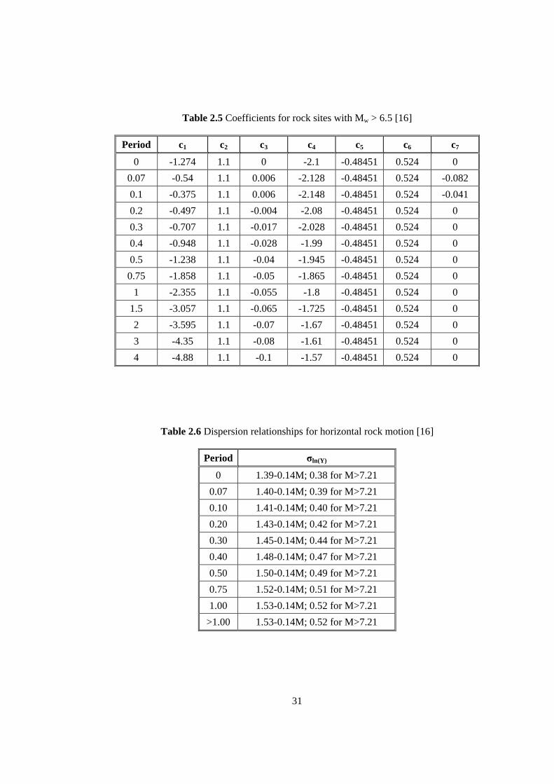
Table 2.5 Coefficients for rock sites with Mw > 6.5 [16]

Period c1 c2 c3 c4 c5 c6 c7

0 -1.274 1.1 0 -2.1 -0.48451 0.524 0 0.07 -0.54 1.1 0.006 -2.128 -0.48451 0.524 -0.082 0.1 -0.375 1.1 0.006 -2.148 -0.48451 0.524 -0.041 0.2 -0.497 1.1 -0.004 -2.08 -0.48451 0.524 0 0.3 -0.707 1.1 -0.017 -2.028 -0.48451 0.524 0 0.4 -0.948 1.1 -0.028 -1.99 -0.48451 0.524 0 0.5 -1.238 1.1 -0.04 -1.945 -0.48451 0.524 0

0.75 -1.858 1.1 -0.05 -1.865 -0.48451 0.524 0 1 -2.355 1.1 -0.055 -1.8 -0.48451 0.524 0

1.5 -3.057 1.1 -0.065 -1.725 -0.48451 0.524 0 2 -3.595 1.1 -0.07 -1.67 -0.48451 0.524 0 3 -4.35 1.1 -0.08 -1.61 -0.48451 0.524 0 4 -4.88 1.1 -0.1 -1.57 -0.48451 0.524 0

Table 2.6 Dispersion relationships for horizontal rock motion [16]

Period σln(Y)

0 1.39-0.14M; 0.38 for M>7.21 0.07 1.40-0.14M; 0.39 for M>7.21 0.10 1.41-0.14M; 0.40 for M>7.21 0.20 1.43-0.14M; 0.42 for M>7.21 0.30 1.45-0.14M; 0.44 for M>7.21 0.40 1.48-0.14M; 0.47 for M>7.21 0.50 1.50-0.14M; 0.49 for M>7.21 0.75 1.52-0.14M; 0.51 for M>7.21 1.00 1.53-0.14M; 0.52 for M>7.21

>1.00 1.53-0.14M; 0.52 for M>7.21

31

Deep Soil Sites: 52

764321 58)lnln 5 .w

·Mcrupw )-M.(ccec(rcMccY w +++−+= (2.19)

where

Y : ground motion parameter (PGA, SA) in g

Mw : moment magnitude

rrup : the closest distance to the rupture surface in km

c1 = -2.17 for strike-slip, -1.92 for reverse and thrust earthquakes

c2 = 1.0

c3 = 1.70

c4 = 2.1863, c5 = 0.32 for M ≤ 6.5

c4 = 0.3825, c5 = 0.5882 for M > 6.5

Table 2.7 Coefficients for deep soil sites [16]

Period c6 Strike-Slip c6 Reverse c7 Standard Error*

0 0 0 0 1.52-0.16M 0.075 0.4572 0.4572 0.005 1.54-0.16M

0.1 0.6395 0.6395 0.005 1.54-0.16M 0.2 0.9187 0.9187 -0.004 1.565-0.16M 0.3 0.9547 0.9547 -0.014 1.58-0.16M 0.4 0.9251 0.9005 -0.024 1.595-0.16M 0.5 0.8494 0.8285 -0.033 1.61-0.16M

0.75 0.701 0.6802 -0.051 1.635-0.16M 1 0.5665 0.5075 -0.065 1.66-0.16M

1.5 0.3235 0.2215 -0.09 1.69-0.16M 2 0.1001 -0.0526 -0.108 1.70-0.16M 3 -0.2801 -0.4905 -0.139 1.71-0.16M 4 -0.6274 -0.8907 -0.16 1.71-0.16M

* Standard error for M > 7 set equal to the value for M = 7

This relationship uses a data set which is composed of primarily California

earthquakes. Geometric mean of the two horizontal components is used to represent PGA

and SA. It is presented for two general site categories: rock (Vs ≈ 620 m/s) and deep soil

(Vs ≈ 310 m/s). There are some limitations to be considered while using this attenuation

relationship. It should not be used to predict ground motions caused by earthquakes

having a moment magnitude less than 4.0 as well as at distances greater than 100 km.

32

2.3.5 Comparison of Attenuation Relationships

Attenuation relationships are compared based on three basic criteria. These are

closest distance to the fault definition, site class definition and spectral acceleration

curves. Comparison is performed to ease selection of proper attenuation relationship

which serves best to the requirements or local conditions.

2.3.5.1 Comparison with respect to distance definitions

Shortest distance to the fault rupture plane is one of the most important parameters

affecting peak ground acceleration at a site. There are different shortest distance

definitions such as rjb, rrup and rhypo proposed by different attenuation relationships. Figure

2.7 shows these shortest distance definitions where rjb is the closest horizontal distance to

the vertical projection of the rupture, rrup is the closest distance to the rupture surface and

rhypo is the hypocentral distance.

Figure 2.7 Distance definitions proposed by attenuation relationships

Each attenuation relationship uses its own definition while calculating the shortest

distance to the fault. The program makes an assumption that fault rupture plane is vertical

and has no depth. As a result of this assumption, fault rupture plane merges to an arc (not

a line due to the curvature of earth) and different closest distance definitions gather around

just one definition, rjb. Table 2.8 presents distance definitions used by each attenuation

relationship.

rrup

rhypo

rjb

Hypocenter

rrup

rjb

Hypocenter

rjb = 0

rruprhypo

rhypo

.

33

Table 2.8 Distance definitions of attenuation relationships

Attenuation relationship Shortest distance definition

Vertical fault rupture (no depth)

Boore et al. [12] rjb rjb → rjb

Gülkan and Kalkan [21] rjb rjb → rjb

Abrahamson & Silva [20] rrup rrup → rjb

Sadigh et al. [16] rrup rrup → rjb

rjb is taken as the shortest distance definition for all four attenuation relationships.

rjb can be expressed as the shortest distance of a point to an arc which is generated by short

line segments in 3D Cartesian coordinates.

2.3.5.2 Comparison with respect to site class definitions

Local site condition is another important parameter affecting peak ground

acceleration at a site. Each attenuation relationship differs in the way that they introduce

local site conditions. While taking into account local site effects, Boore et al. [12] and

Gülkan & Kalkan [21] relationships make use of the average shear wave velocity whereas

Sadigh et al. [16] and Abrahamson & Silva [20] refer to a simplified classification: deep

soil and rock. Table 2.9 summarizes the ways of introducing local site conditions for each

model and Table 2.10 presents average shear wave velocities proposed by developers of

each attenuation relationship.

Table 2.9 Inclusion of local site effects for each attenuation relationship

Boore et al. [12] Gülkan and Kalkan [21]

Abrahamson and Silva [20] Sadigh et al. [16]

While introducing local site conditions, Uses average Vs

and is capable of

generating spectra

for all reasonable

values of Vs

(quantitative)

Uses average Vs

and is capable of

generating spectra

for all reasonable

values of Vs

(quantitative)

Generates spectra

only for Rock and

Deep Soil sites

(not functional for

intermediate sites)

(qualitative)

Generates spectra

only for Rock and

Deep Soil sites

(not functional for

intermediate sites)

(qualitative)

34

Table 2.10 Proposed average shear wave velocities for each attenuation relationship

Boore et al. [12] Gülkan and Kalkan [21]

Abrahamson and Silva [20] Sadigh et al. [16]

Proposed average shear wave velocities

ave Vs = 620 m/s

(Rock)

ave Vs = 700 m/s

(Rock) Rock

(ave Vs = 620 m/s)

Rock

(ave Vs = 620 m/s) ave Vs = 310 m/s

(Deep Soil)

ave Vs = 400 m/s

(Soil)

Vs < 180 m/s

(Soft Soil)

ave Vs = 200 m/s

(Soft Soil)

Deep Soil

(ave Vs = 310 m/s)

Deep Soil

(ave Vs = 310 m/s)

2.3.5.3 Comparison with respect to spectral acceleration curves

The spectral acceleration values produced by different attenuation relationships

are compared in this part. Analyses were performed for different moment magnitudes,

closest distances, site conditions and attenuation relations. Table 2.11 presents

combinations that were employed during analysis process. 112 runs were made but only

the representative ones are selected to be presented here.

Table 2.11 Analyses performed in order to compare spectral acceleration curves

Abrahamson and Silva [20] Boore et al. [12] Gülkan and

Kalkan [21] Sadigh et al. [16]

Mw 5.5 7 5.5 7 5.5 7 5.5 7 5.5 7 5.5 7 5.5 7 5.5 7

D (km) Rock Soil Rock Soil Rock Soil Rock Soil 1 √ √ √ √ √ √ √ √ √ √ √ √ √ √ √ √ 5 √ ● √ ● √ ● √ ● √ ● √ ● √ ● √ ●

10 √ √ √ √ √ √ √ √ √ √ √ √ √ √ √ √

20 √ √ √ √ √ √ √ √ √ √ √ √ √ √ √ √ 30 √ √ √ √ √ √ √ √ √ √ √ √ √ √ √ √

50 √ ● √ ● √ ● √ ● √ ● √ ● √ ● √ ●

100 √ √ √ √ √ √ √ √ √ √ √ √ √ √ √ √ √ : analysis performed , ● : selected to be representative for all other cases

35

Values obtained for moment magnitude 7 were used and the resulting graphs are

presented in Figures 2.8 – 2.13. Comparison is initially performed in terms of peak ground

acceleration (PGA), short-period spectral acceleration (Sa at T = 0.3 s) and long-period

spectral acceleration (Sa at T = 1.0 s) variations with respect to closest distance to the fault

rupture for rock and soil sites.

Considering PGA variation with respect to distance, Boore et al. [12] (B) and

Gülkan & Kalkan [21] (GK) relationships attenuate more slowly as compared to

Abrahamson & Silva [20] (AS) and Sadigh et al. [16] (S) relations for both rock and soil

sites. Figure 2.8 shows that AS and S relations give higher PGA values at rock sites

(PGArock) when compared to the values proposed by B and GK relationships. For soil

sites, all attenuation relations except GK yield quite similar results whereas GK gives

lower values for near field and higher values for far field.

0.01

0.1

1

1 10

Closest Distance (km)

PG

A (g

)

100

Abrahamson and Silva (1997)Boore et al (1997)Gulkan and Kalkan (2002)Sadigh et al (1997)

Figure 2.8 Comparison of attenuation relationships for rock sites with Mw = 7

36

0.01

0.1

1

1 10 100

Closest Distance (km)

PG

A (g

)

Abrahamson and Silva (1997)Boore et al (1997)Gulkan and Kalkan (2002)Sadigh et al (1997)

Figure 2.9 Comparison of attenuation relationships for soil sites with Mw = 7

Considering PGA variation with respect to site conditions, PGA values calculated

by using B and GK relationships at rock sites are lower than the values found by same

relations at soil sites (PGAsoil). In case of AS and S relations, PGArock values are higher

than PGAsoil values and this inequality changes direction as closest distance to the fault

rupture increases.

For a better understanding of each attenuation relationship, spectral acceleration

values at periods of 0.3 s and 1.0 s are also plotted and presented in Figures 2.10 and 2.11.

The graphs demonstrate that the variation is almost same as in the case of PGA. These

spectral acceleration values at T = 0.3 s and T = 1.0 s (Sa@T=0.3 and Sa@T=1.0) are

critical and they are selected as representative values of short period and long period

respectively. Only these two values are required to generate a demand spectrum

resembling the original curve proposed by the attenuation relationship.

37

0.01

0.1

1

10

1 10

Closest Distance (km)

SA@

T=0.

3 (g

)

100

Abrahamson and Silva (1997)Boore et al (1997)Gulkan and Kalkan (2002)Sadigh et al (1997)

(a)

0.01

0.1

1

10

1 10

Closest Distance (km)

SA@

T=0.

3 (g

)

100

Abrahamson and Silva (1997)Boore et al (1997)Gulkan and Kalkan (2002)Sadigh et al (1997)

(b)

Figure 2.10 Comparison of Sa values at T=0.3s for Mw = 7. (a) rock site, (b) soil site

38

0.01

0.1

1

1 10 100

Closest Distance (km)

SA

@T=

1 (g

)

Abrahamson and Silva (1997)Boore et al (1997)Gulkan and Kalkan (2002)Sadigh et al (1997)

(a)

0.01

0.1

1

10

1 10

Closest Distance (km)

SA@

T=1

(g)

100

Abrahamson and Silva (1997)Boore et al (1997)Gulkan and Kalkan (2002)Sadigh et al (1997)

(b)

Figure 2.11 Comparison of Sa values at T=1.0s for Mw = 7. (a) rock site, (b) soil site

39

Secondly, another comparison is made for spectral curves obtained at distances of

5 and 50 km for rock and soil sites with an assumed moment magnitude of 7.0. Figure

2.12 shows that there is significant difference between short-period acceleration values of

all four attenuation relationships when local site is rock. Long-period acceleration values

follow a similar trend. AS and S relations produce almost same curves excluding the

interval of 0.1 s and 0.4 s. GK relationship yields the lower bound curve whereas AS gives

the upper bound.

In case of soil site (Figure 2.13), peaks of short-period acceleration values vary

between 0.9g and 1.1g and long-period accelerations for all attenuation relationships are

quite compatible except GK relationship which produced lower values. PGA values are

between 0.35g and 0.44g. Unlike rock sites, B relationship forms the upper bound curve

since AS and S relations give lower spectral acceleration values for soil sites as compared

to their proposed PGArock.

5 km (Rock)

0

0.2

0.4

0.6

0.8

1

1.2

1.4

0 0.2 0.4 0.6 0.8 1 1.2 1.4 1.6 1.8 2

Period (s)

SA

(g)

Abrahamson and Silva (1997)Boore et al (1997)Gulkan and Kalkan (2002)Sadigh et al (1997)

Figure 2.12 Spectral acceleration curves for rock site with Mw = 7 and d = 5 km

40

5 km (Soil)

0

0.2

0.4

0.6

0.8

1

1.2

1.4

0 0.2 0.4 0.6 0.8 1 1.2 1.4 1.6 1.8 2

Period (s)

SA (g

)

Abrahamson and Silva (1997)Boore et al (1997)Gulkan and Kalkan (2002)Sadigh et al (1997)

Figure 2.13 Spectral acceleration curves for soil site with Mw = 7 and d = 5 km

When closest distance to the fault rupture increases, spectral acceleration curves

proposed by different attenuation relationships become similar which can be observed

from Figures 2.14 and 2.15. Another observation is that GK attenuation relationship

produces approximately 1.4 times larger values. This should be expected because GK

relation attenuates slowly and yields larger spectral acceleration values for distant sites

independent of site conditions. AS, S and B relationships are almost equivalent for rock

sites and differ slightly at periods greater than 0.6 s in case of soil sites.

In summary, AS and S relations show similar behavior as it is also the case for B

and GK relationships. For all cases, GK attenuation relation follows general trend but

produces considerably different spectral acceleration curves since it reflects the character

of earthquakes happened in Turkey. So, it might be better to employ GK attenuation

relationship in order to construct spectral acceleration curves for the regions in Turkey.

41

50 km (Rock)

0

0.05

0.1

0.15

0.2

0.25

0.3

0.35

0 0.2 0.4 0.6 0.8 1 1.2 1.4 1.6 1.8 2

Period (s)

SA

(g)

Abrahamson and Silva (1997)Boore et al (1997)Gulkan and Kalkan (2002)Sadigh et al (1997)

Figure 2.14 Spectral acceleration curves for rock site with Mw = 7 and d = 50 km

50 km (Soil)

0

0.05

0.1

0.15

0.2

0.25

0.3

0.35

0 0.2 0.4 0.6 0.8 1 1.2 1.4 1.6 1.8 2

Period (s)

SA (g

)

Abrahamson and Silva (1997)Boore et al (1997)Gulkan and Kalkan (2002)Sadigh et al (1997)

Figure 2.15 Spectral acceleration curves for soil site with Mw = 7 and d = 50 km

42

2.4 COMPUTATION OF DISPLACEMENT DEMAND

Seismic risk assessment methodology has another important component which is

the computation of displacement demand. During this process, the displacement demand

imposed by the probable or deterministic earthquakes on the structure is determined by

employing different procedures each of which has its own advantages and drawbacks. The

software developed uses three wide-spread methodologies. The theoretical background for

each methodology is presented in the following sections. The procedures are excerpted

from “Seismic Evaluation and Retrofit of Concrete Buildings (ATC-40)” [8], “Prestandard

and Commentary for the Seismic Rehabilitation of Buildings (FEMA-356)” [19] and

“Capacity-Demand-Diagram Methods for Estimating Seismic Deformation of Inelastic

Structures: SDF Systems (Chopra & Goel)” [22] for instructive purposes. Inevitably, the

tables and formulae, proposed by ATC-40, FEMA-356 and Chopra & Goel included in

this study have minor differences in the way they are presented. Interested reader is

referred to referenced material for further details and explanations.

2.4.1 Capacity Spectrum Method (ATC-40 Procedure B)

The analysis procedure proposed by ATC-40 [8] mainly focuses on capacity

spectrum method which is one of the nonlinear static analysis procedures. In general,

simplified nonlinear static analysis procedures require three components: capacity,

demand and performance.

Capacity: It is the representation of the building response.

Demand: It is the representation of the seismic effect.

Performance: It is a point that represents the condition of the building to the given

demand.

ATC-40 defines three different structural behavior types. Since these types will be

declared frequently in the subsequent paragraphs, it should be better to present the

classification scheme here.

Table 2.12 Structural behavior types defined by ATC-40 [8]

Shaking

Duration

Essentially New

Building

Average Existing

Building

Poor Existing

Building

Short Type A Type B Type C Long Type B Type C Type C

43

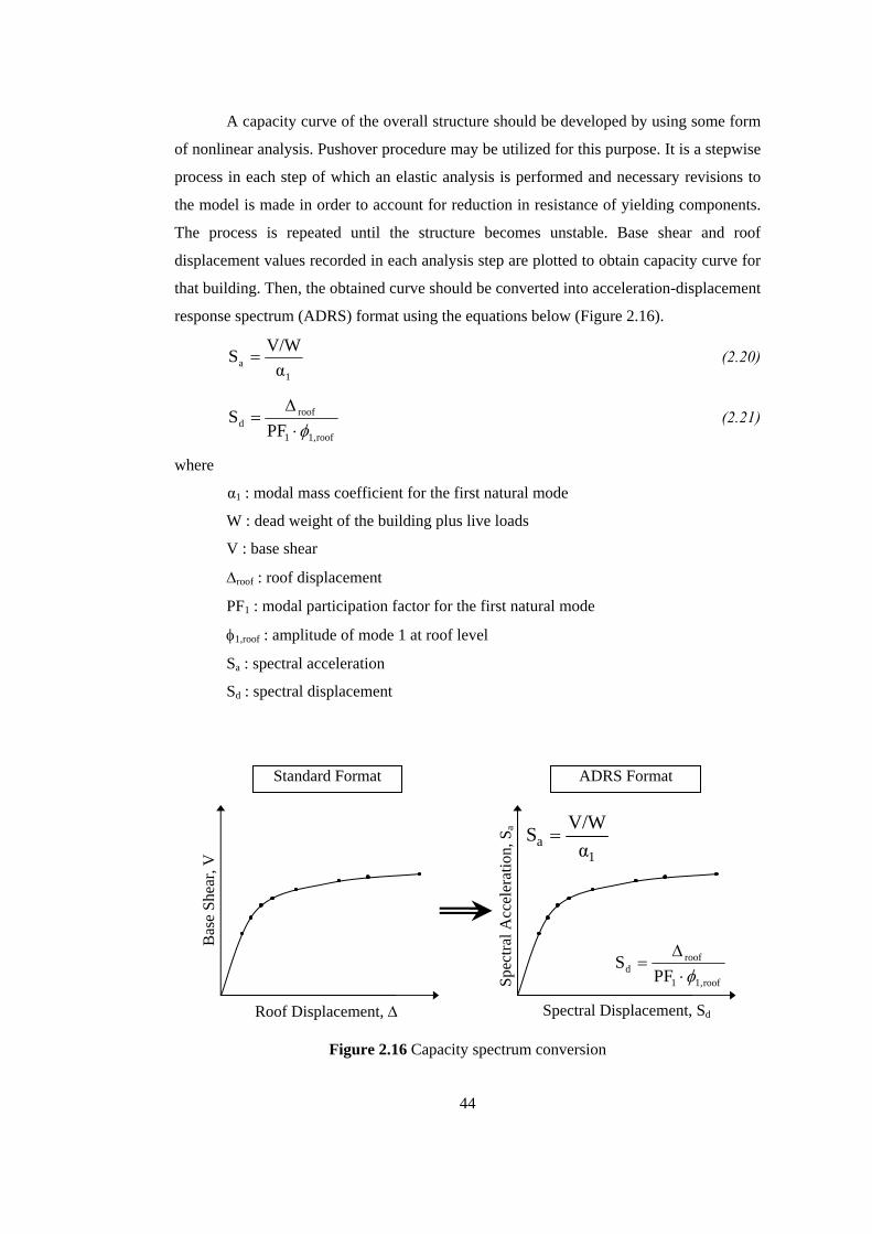
A capacity curve of the overall structure should be developed by using some form

of nonlinear analysis. Pushover procedure may be utilized for this purpose. It is a stepwise

process in each step of which an elastic analysis is performed and necessary revisions to

the model is made in order to account for reduction in resistance of yielding components.

The process is repeated until the structure becomes unstable. Base shear and roof

displacement values recorded in each analysis step are plotted to obtain capacity curve for

that building. Then, the obtained curve should be converted into acceleration-displacement

response spectrum (ADRS) format using the equations below (Figure 2.16).

1a α

V/WS = (2.20)

roof1,1

roofd PF

Sφ⋅

∆= (2.21)

where

α1 : modal mass coefficient for the first natural mode

W : dead weight of the building plus live loads

V : base shear

∆roof : roof displacement

PF1 : modal participation factor for the first natural mode

φ1,roof : amplitude of mode 1 at roof level

Sa : spectral acceleration

Sd : spectral displacement

Figure 2.16 Capacity spectrum conversion

Bas

e Sh

ear,

V

Roof Displacement, ∆

Spec

tral A

ccel

erat

ion,

Sa

Standard Format ADRS Format

1a α

V/WS =

roof1,1

roofd PF

Sφ⋅

∆=

Spectral Displacement, Sd

44

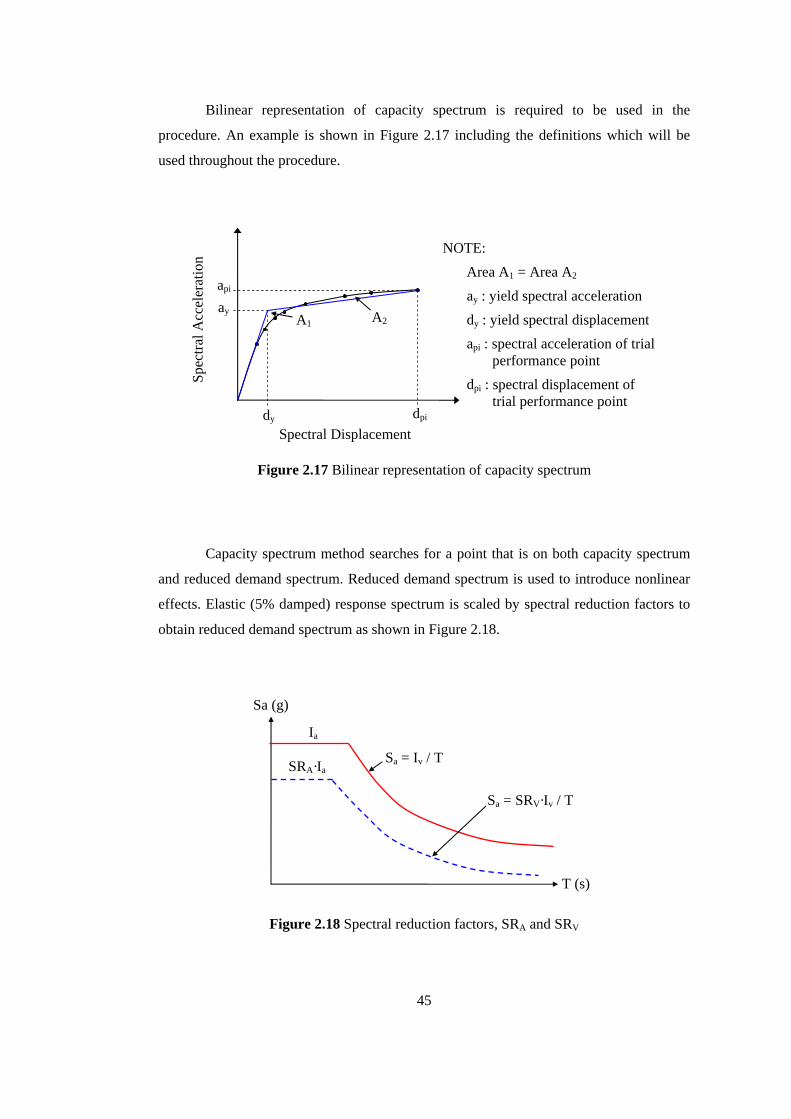
Bilinear representation of capacity spectrum is required to be used in the

procedure. An example is shown in Figure 2.17 including the definitions which will be

used throughout the procedure.

NOTE:

Spec

tral A

ccel

erat

ion

Area A1 = Area A2api ay : yield spectral acceleration

Figure 2.17 Bilinear representation of capacity spectrum

Capacity spectrum method searches for a point that is on both capacity spectrum

and reduced demand spectrum. Reduced demand spectrum is used to introduce nonlinear

effects. Elastic (5% damped) response spectrum is scaled by spectral reduction factors to

obtain reduced demand spectrum as shown in Figure 2.18.

Figure 2.18 Spectral reduction factors, SRA and SRV

Sa (g)

T (s)

Ia

Sa = Iv / T SRA·Ia

Sa = SRV·Iv / T

Spectral Displacement

ay

dy dpi

A1 A2 dy : yield spectral displacement api : spectral acceleration of trial performance point dpi : spectral displacement of trial performance point

45

Spectral reduction factors are given in terms of effective damping. Effective

damping may be calculated using the following equation.

5βκβ 0eff +⋅= (2.22)

where

βeff : effective damping. This value should not be greater than 40% for Type A,

9% for T

the structure (5%)

viscous damping

2 ype B and 20% for Type C.

5 : viscous damping inherit in

β0 : hysteretic damping represented as equivalent

piypiy )add63.7(a −

pipi0 da

β = (2.23)

κ : a modification factor for the simulation of probable imperfections in real

uilding

Table 2.13 Values for damping modification factor, κ (ATC-40 [8])

Behavior Type β0 (percent) κ

b hysteresis loops, which may be pinching or degrading. Table 2.13 presents values

for κ depending on structural behavior type and equivalent viscous damping.

Structural

≤ 16.25 1.0

Type A > 16.25

)d(a)add(a0.51

1.13pipi

piypiy −−

≤ 25 0.67

Type B > 25

)d(a)add0.446(a y0.845

pipi

piypi −−

Type C Any value 0.33

pectral reduction factors are calculated using the following equations.

S

2.12)ln(β0.683.21SR eff⋅−

≈ A (2.24)

1.65)ln(β0.412.31SR eff

V⋅−

≈ (2.25)

46

Note that SRA and SRV values found by the above formulae should not be l

than the values provided in Table 2.14.

ues for SRA and SRV proposed by ATC-40 [8]

ess

Table 2.14 Minimum allowable val

Structural Behavior Type SRA SRV

Type A 0.33 0.50

Type B 0.44 0.56

Type C 0.56 0.67

fter reducing the elastic demand curve by using spectral reduction factors, it

should be also converted into ADRS format. Conversion of demand curve from standard

format

A

into ADRS format is shown in Figure 2.19.

Figure 2.19 Conversion of demand spectrum

Spec

tral A

ccel

erat

ion,

Sa

Spectral Displacement, Sd

Standard Format ADRS Format

Period, T

aSp

ectra

l Acc

eler

atio

n, S

Ta Tb

Ta

Tb

a

2a2 TS

4πd1S =

dSπ2T = S

47

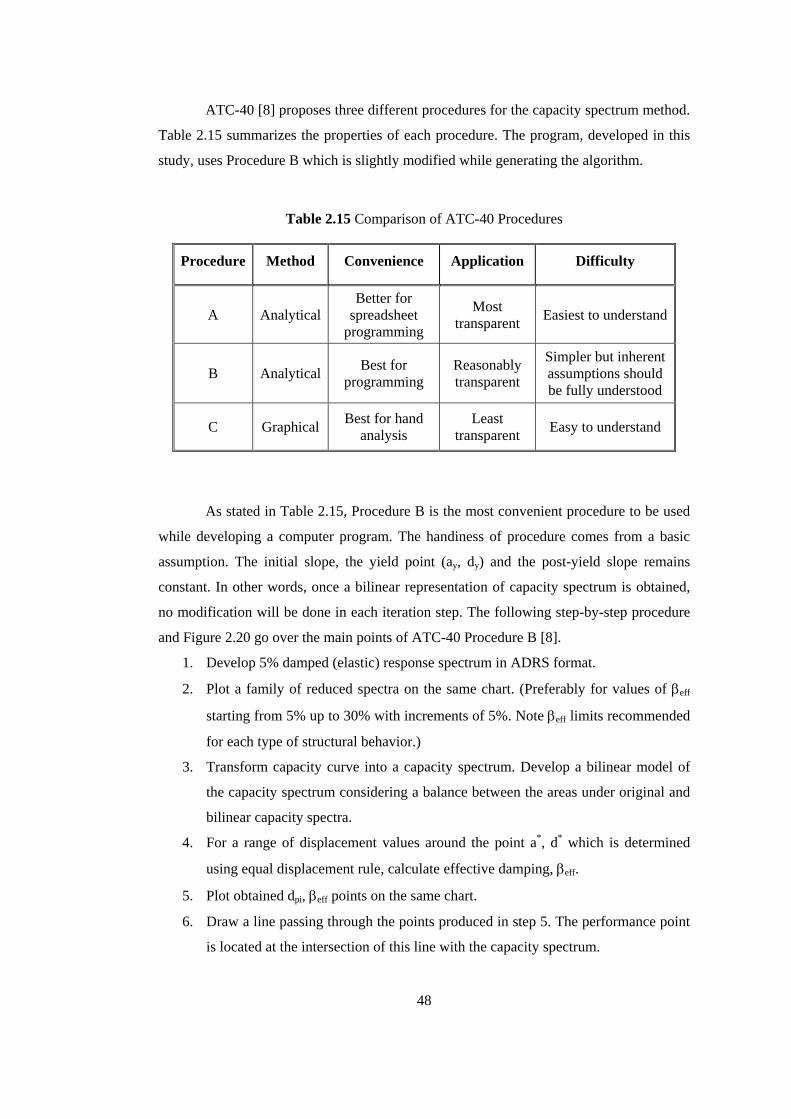
ATC-40 [8] proposes three different procedures for the capacity spectrum method.

Table 2

Table 2.15 Comparison of ATC-40 Procedures

Procedure Method Convenience Application Difficulty

.15 summarizes the properties of each procedure. The program, developed in this

study, uses Procedure B which is slightly modified while generating the algorithm.

A Analytical spreadsheet p

Most transparent Easiest to understand

Better for

rogramming

B Analytical programming Reasonably Simpler but inherent Best for transparent assumptions should

be fully understood

C Graphical transparent Best for hand

analysis Least Easy to understand

As stated in Table 2.15, Procedure B is the most convenient procedure to be used

while d

mat.

r values of βeff

3. city spectrum. Develop a bilinear model of

4. ent values around the point a*, d* which is determined

5.

d in step 5. The performance point

is located at the intersection of this line with the capacity spectrum.

eveloping a computer program. The handiness of procedure comes from a basic

assumption. The initial slope, the yield point (ay, dy) and the post-yield slope remains

constant. In other words, once a bilinear representation of capacity spectrum is obtained,

no modification will be done in each iteration step. The following step-by-step procedure

and Figure 2.20 go over the main points of ATC-40 Procedure B [8].

1. Develop 5% damped (elastic) response spectrum in ADRS for

2. Plot a family of reduced spectra on the same chart. (Preferably fo

starting from 5% up to 30% with increments of 5%. Note βeff limits recommended

for each type of structural behavior.)

Transform capacity curve into a capa

the capacity spectrum considering a balance between the areas under original and

bilinear capacity spectra.

For a range of displacem

using equal displacement rule, calculate effective damping, βeff.

Plot obtained dpi, βeff points on the same chart.

6. Draw a line passing through the points produce

48

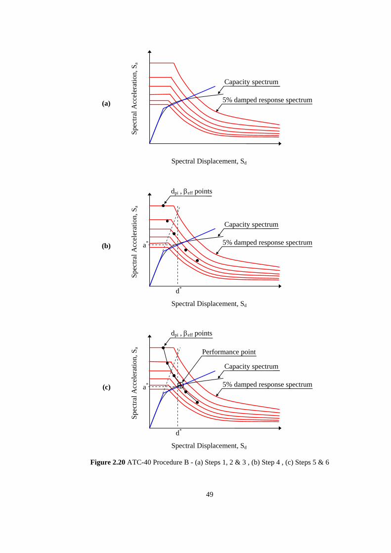
Figure 2.20 ATC-40 Procedure B - (a) Steps 1, 2 & 3 , (b) Step 4 , (c) Steps 5 & 6

(c) 5% damped response spectrum

Spec

tral A

ccel

erat

ion,

Sa

Spectral Displacement, Sd

Capacity spectrum

d*

a*

dpi , βeff points

Performance point

(b) 5% damped response spectrum

a

Spectral Displacement, Sd

Capacity spectrum

d*

a*

Spec

tral A

ccel

erat

ion,

S

dpi , βeff points

(a) 5% damped response spectrum

Spectral Displacement, Sd

Capacity spectrum

Spec

tral A

ccel

erat

ion,

Sa

49

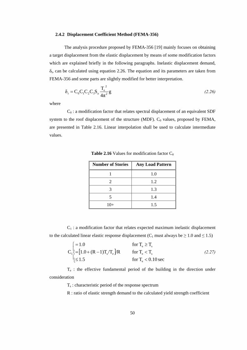
2

] mainly focuses on obtaining

a target displacement from the elastic displacement by means of some modification factors

which a

.4.2 Displacement Coefficient Method (FEMA-356)

The analysis procedure proposed by FEMA-356 [19

re explained briefly in the following paragraphs. Inelastic displacement demand,

δt, can be calculated using equation 2.26. The equation and its parameters are taken from

FEMA-356 and some parts are slightly modified for better interpretation.

g4πTSCCCCδ 2

2e

a3210t = (2.26)

where

C0 : a modification factor that relates spectral displacement of an equivalent SDF

displacement of the structure (MDF). C values, proposed by FEMA,

Table 2.16 Values for modification factor C0

system to the roof 0

are presented in Table 2.16. Linear interpolation shall be used to calculate intermediate

values.

Number of Stories Any Load Pattern

1 1.0

2 1.2

3 1.3

5 1.4

10+ 1.5

C1 : a modification factor that relates expected maximum inelastic displacement

to the calculated linear elastic response displacement (C must always be ≥ 1.0 and ≤ 1.5)

⎨<≤ sec 0.10Tfor 1.5 e

sees1

Te : the effective fundamental period of the building in the direction under

consideration

tio of elastic strength demand to the calculated yield strength coefficient

1

[ ]⎪⎧

<−+=≥=

TTfor /R/T1)T(R1.0TTfor 1.0

Cse

(2.27)⎪⎩

Ts : characteristic period of the response spectrum

R : ra

50

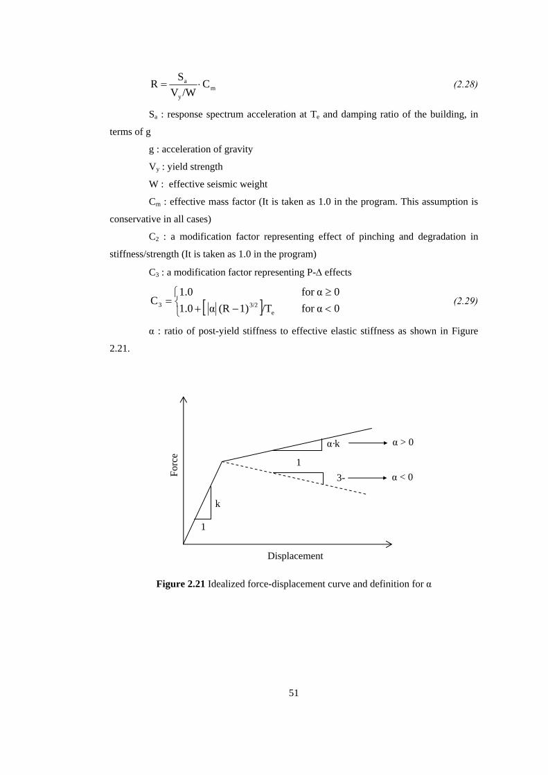
my

a CSR ⋅= (2.28)/WV

Sa : response spectrum acceleration at Te and damping ratio of the building, in

: acceleration of gravity

ic weight

s taken as 1.0 in the program. This assumption is

tion factor representing effect of pinching and degradation in

effects

terms of g

g

Vy : yield strength

W : effective seism

Cm : effective mass factor (It i

conservative in all cases)

C2 : a modifica

stiffness/strength (It is taken as 1.0 in the program)

C3 : a modification factor representing P-∆

[ ]⎩⎨⎧ ≥ 0αfor 1.0

<−+=

0αfor /T1)(R α1.0C

e3/23 (2.29)

α : ratio of post-yield stiffness to effective elastic stiffness as shown in Figure

.21.

α

2

Figure 2.21 Idealized force-displacement curve and definition for

α·k

3- 1

1

k

α > 0

α < 0

Displacement

Forc

e

51

2.4.3 Constant Ductility Procedure (Chopra and Goel)

An improvement to the ATC-40 [8] procedures is proposed by Chopra and Goel.

This improved method utilizes well-known constant ductility design spectrum that is why

it is declared as ‘constant ductility procedure’ throughout this study. The main difference

between ATC-40 procedures and the improved ones is the way in which the demand is

calculated. ATC-40 procedures employ equivalent linear systems whereas the improved

ones enable to analyze an inelastic system.

There are three versions of improved procedures; Procedure A, B and Numerical.

Procedures A and B are very similar to ATC-40 procedures A and B. They reduce the

errors in the ATC-40 procedures by keeping hold of graphical attractiveness of both

methods [22]. The numerical version is a reworked copy of the improved procedures and

facilitates programmable algorithm generation. Since it is better for programming, it is

preferred while developing the software.

The numerical version requires usage of Ry - µ - Tn equations. There are three

different sets of equations proposed by the following researchers:

• Newmark-Hall [23]

• Krawinkler and Nassar [24]

• Vidic, Fajfar and Fischinger [25]

For the sake of completeness, each equation set is explained briefly in the

subsequent paragraphs.

Newmark-Hall [23] developed Ry - µ - Tn equations based on elastoplastic

systems. The reversed equations, giving µ as a function of Ry, are (Chopra [26]):

⎪⎪⎪

⎩

⎪⎪⎪

⎨

⎧

>

<<

<<+<<+

<

=

cny

cnc'yn

c

c'nb2

y

bnaβ / 2

y

an

TTR

TTTRTT

TTT2 / )R(1TTT2 / )R(1

TTUndefined

µ (2.30)

where

(2.31) )/T)/ln(T/Tln(Tβ aban=

Krawinkler and Nassar [24] developed Ry - µ - Tn equations based on earthquake

response of bilinear systems. The equations, giving µ as a function of Ry, are:

52

1)(Rc11µ c

y −+= (2.32)

where

n

an

an

n Tb

T1Tα),c(T ++

= (2.33)

α : the coefficient representing slope of the yielding branch (αk) in terms of

initial stiffness, k (presented previously in Figure 2.21)

a and b coefficients depend on value of α. Table 2.17 presents a and b

coefficients corresponding to different α values.

Table 2.17 Values of a and b coefficients

α a b

0 1 0.42 0.02 1 0.37

0.10 0.8 0.29

Vidic, Fajfar and Fischinger [25] developed Ry - µ - Tn equations based on

earthquake response of bilinear systems. The equations, giving µ as a function of Ry, are:

[ ]⎪⎩

⎪⎨

⎧

>−+

≤⎥⎦

⎤⎢⎣

⎡−+

=

0n1.053

y

0n

1.053

n

0y

TT1)0.74(R1

TTTT

1)0.74(R1µ (2.34)

where

(2.35) cc0.2

0 TT0.75µT ≤=

Since T0 also depends on ductility, the procedure requires an iterative solution. A

simplifying assumption of T0 = Tc may be used for non-iterative solution.

Numerical version of the improved methods is composed of the following steps.

Figure 2.22 also describes some steps graphically.

1. Develop 5% damped (elastic) response spectrum in standard format.

2. Transform capacity curve into a capacity spectrum. Develop a bilinear model of

the capacity spectrum considering a balance between the areas under original and

bilinear capacity spectra.

53

3. Calculate Ti from 2π(dy. / ay)0.5

4. Using 5% damped response spectrum, find spectral acceleration A for period Ti.

5. Calculate Ry using the equation Ry = A / ay.

6. Select the set of Ry - µ - Tn equations to be used in the analysis and compute µ

using the selected equation set.

7. Calculate Sdi using the equation (Sdi = dy · µ) → Sdi is the performance point.

Figure 2.22 Steps 2, 3 & 4 of numerical version for the improved procedures

Step 2 & 3

Spec

tral A

ccel

erat

ion,

Sa

Spectral Displacement, Sd

ay

apiTi

amax

dmaxdpidy

Step 4

Spec

tral A

ccel

erat

ion,

Sa 5% damped response spectrum

Period, T Ti

A

54

CHAPTER 3

STRUCTURE OF THE SEISMIC RISK ANALYSIS SOFTWARE

3.1 INTRODUCTION

This study mainly focuses on developing seismic risk analysis software. The

software developed uses the deterministic approach to predict the probable damage

distribution for a specified region caused by a deterministic earthquake. Fault locations

and building stock layouts are entered in terms of latitudes and longitudes. Results are also

provided in latitudes and longitudes which makes mapping of results simpler and faster. It

is capable of handling four attenuation relationships and three displacement demand

computation methods. These relationships and methods are explained in Chapter 2.

Development of the software is basically performed by dividing the overall

process into smaller sub-processes. Each sub-process, namely component, has made

programming and debugging processes simpler and more efficient. Since the source codes

of each component as well as the software itself reflect only programming details, it

would be a vain attempt to include these codes. As a replacement for source codes, the

step-by-step algorithms are provided to demonstrate and understand what the software

does behind the nice-looking interface. Structure of the software with its components is

discussed in depth in section 3.2.

3.2 SOFTWARE COMPONENTS

The name “Seismic Risk Analysis Software” is given to the software developed.

From now on, it will be frequently denoted by the initial capitals as “SRAS”. SRAS has a

modular structure that is deliberately chosen to ease error handling process and constitute

55

a well-built base for further modifications and upgrades. These partitions or components

provide an open structure to the software by making it clearer and easier to use. Since

SRAS has been developed just for educational proposes, it may give the impression of

being much more instructive than necessary for experienced users.

Just as a reminder, SRAS is a computer program and all well-known facts about

commercial software are also valid for SRAS. What is given as an input will be returned

as an output of same quality. In other words, if garbage enters, garbage will be out. So, it

is the user responsibility to verify the reliability of the results produced by SRAS.

Flowchart of the software is presented in Figure 3.1. SRAS is basically composed

of three major modules that are common to all computer programs. These are input,

calculation and output components. Each component has different numbers of sub-

categories. This section is devoted to explaining these major components including their

subdivisions.

As an overview, the software entails five data sets to start analysis. Building

inventory data, attenuation relationship data, scenario earthquake data, capacity curves for

each building type and analysis method data are the fundamental inputs to SRAS. Reliable

building inventory data is a must to obtain realistic results for the defined scenario

earthquakes assuming that the attenuation relationships and analysis methods yield

dependable results.

After completion of input data, the calculation phase starts. This phase is

composed of three parts, which are demand calculation, performance calculation and

damage estimation. Demand calculation part, initially, finds the shortest distance between

each building in the region and the scenario earthquake fault and then generates smoothed

acceleration response spectrum expected under each building. Subsequently, performance

calculation module computes performance point using the generated demand curve and

provided capacity curve for each building. Finally, damage estimation module predicts the

performance of each building under the scenario earthquake induced forces. Results

obtained from the analysis are exported to a database file or displayed on the screen. And

also, a report is created which includes the site based distribution of damage and all input

data.

56

Seismic Risk Analysis Software (SRAS)

Building Inventory Data

Scenario Earthquake Data

Capacity Curve Data

Analysis Method Data

Attenuation Relationship Data

Demand Calculation

Performance Calculation

Damage Estimation

Screen Display

Report Generation

Exporting Results

CALCULATION

INPUT

OUTPUT

Fault Model (rupture length, geometry, location)Moment Magnitude

ATC-40 Procedure BConstant DuctilityFEMA-356

Site Classification SchemeAttenuation Relationship Abrahamson & Silva Boore et al Gulkan & Kalkan Sadigh et al

Site IDSite LabelBuilding LabelLatitudeLongitudeSite ClassNumber of StoriesBuilding TypeNumber of BuildingsConstruction YearCondition

Calculating Closest Distance to the FaultCalculating

Peak Ground Acceleration@ T = 0.3 s@ T = 1.0 s

Demand Spectrum Generation

Calculating Performance Point by utilizing:Demand SpectrumCapacity Spectrum (taken as input)Analysis Method (taken as input)

Estimating Damage:Based on Sd limitsBased on Damage Curves

Generating Report which includes:All Input DataClosest Distance to the FaultDemand Parameters (PGA, Sa values)Performance PointDamage Distribution within Each Site

in one of the following formats:Microsoft Word Document (*.doc)Text File (*.txt)

Exporting Results as:Microsoft Access Database (*.mdb)Microsoft Excel Worksheet (*.xls)

Figure 3.1 Flowchart for SRAS

57

3.2.1 Input Components

SRAS needs five major input components in order to be able to start analysis.

These input components are building inventory, capacity curves, scenario earthquake,

attenuation relationship and analysis method. Each of these components has vital

importance in predicting a realistic damage distribution for the region under consideration.

In the following paragraphs, these components will be covered in details to ensure proper

input to SRAS.

3.2.1.1 Building Inventory Data

Seismic risk analysis software requires building stock information which is the

fundamental input for risk analysis. Accuracy of analysis results depend on not only the

methods or attenuation relationships used but also the reliability of the building database.

Using reliable sources in collecting regional building data is crucial to obtain realistic and

dependable results. This data gathering process may not be a serious problem in developed

countries which probably have completed digitization of the entire country including

transportation, power and water supply distribution and communication networks. These

high resolution digital maps give all detailed information about the region under

consideration. In the case of undeveloped or developing countries, the process seems quite

challenging. Aside from detailed regional digital maps, it is even impossible to obtain a

sketchy digital map only showing the district boundaries. After overcoming the difficulties

in obtaining building inventory information, a preliminary screening is required to prepare

this raw data as an input for SRAS. Building inventory input file should include the

characteristics of buildings in the region. Building characteristics refer to the properties of

each building that are going to be utilized during the analysis. There are 12 properties

required for each building:

1. Site ID

2. Site Label

3. Building Label

4. Latitude

5. Longitude

6. Site Class or Average Vs

7. Number of Stories

8. Building Type

9. Number of Buildings

10. Construction Year

11. Apparent Condition

12. Information

Site ID is numerical representation of Site Label. Site Label is the name of the

sub-district or district depending on the resolution of digital map and building inventory.

58

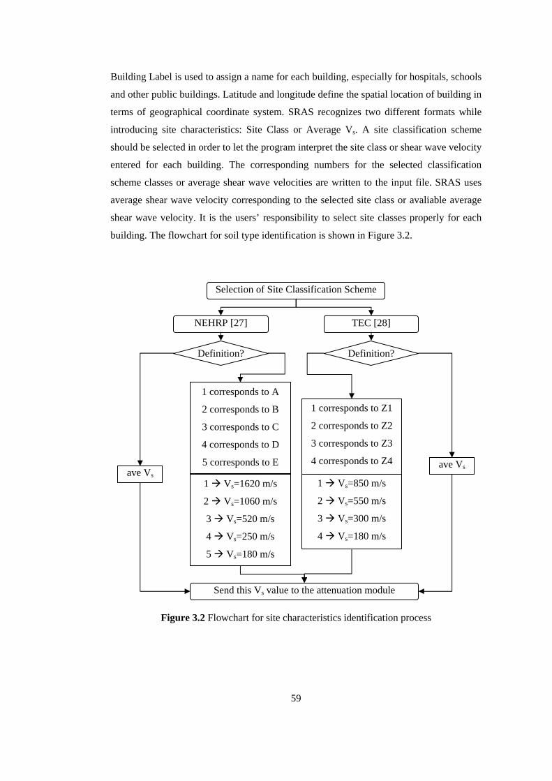
Building Label is used to assign a name for each building, especially for hospitals, schools

and other public buildings. Latitude and longitude define the spatial location of building in

terms of geographical coordinate system. SRAS recognizes two different formats while

introducing site characteristics: Site Class or Average Vs. A site classification scheme

should be selected in order to let the program interpret the site class or shear wave velocity

entered for each building. The corresponding numbers for the selected classification

scheme classes or average shear wave velocities are written to the input file. SRAS uses

average shear wave velocity corresponding to the selected site class or avaliable average

shear wave velocity. It is the users’ responsibility to select site classes properly for each

building. The flowchart for soil type identification is shown in Figure 3.2.

Selection of Site Classification Scheme

NEHRP [27] TEC [28]

Definition? Definition?

1 corresponds to A 1 corresponds to Z1 2 corresponds to B 2 corresponds to Z2 3 corresponds to C 3 corresponds to Z3 4 corresponds to D 4 corresponds to Z4 5 corresponds to E ave Vs

ave Vs1 Vs=850 m/s 1 Vs=1620 m/s

2 Vs=550 m/s 2 Vs=1060 m/s

3 Vs=300 m/s 3 Vs=520 m/s

4 Vs=180 m/s 4 Vs=250 m/s

5 Vs=180 m/s

Send this Vs value to the attenuation module

Figure 3.2 Flowchart for site characteristics identification process

59

There are two site classification schemes used in the program: NEHRP [27] and

TEC [28]. Each of these site classification schemes has its own qualitative and

quantitative definitions as shown in Tables 3.1 and 3.2.

Table 3.1 NEHRP [27] site classification scheme

Mean Vs (m/s) Class Name General Description

Min. Ave. Max.

A HARD ROCK (e.g. metamorphic rocks with very widely spaced fractures)

1500 1620 -

B ROCK (e.g. granites, igneous rocks, conglomerates, sandstones, and shales with close to widely spaced fractures)

760 1060 1500

C VERY DENSE SOIL and SOFT ROCK (e.g. soft igneous sedimentary rocks, sandstones, and shales, gravels, and soils with >20% gravel)

360 520 760

D STIFF SOIL (e.g. loose to very dense sands, silt loams and sandy clays, and medium stiff to hard clays and silty clays (15 < N < 50 blows/ft))

180 250 360

E SOFT SOILS (e.g. loose submerged fills and very soft to soft (N < 15 blows/ft) clays and silty clays > 3m (10 ft) thick)

- 140 180

Table 3.2 TEC [28] site classification scheme

Mean Vs (m/s) Class Name General Description

Min. Ave. Max.

Z1 FIRM to HARD ROCKS (e.g. rock, very stiff clay, very dense sands) 700 850 -

Z2 GRAVELLY SOILS and SOFT to FIRM ROCKS (e.g. tuffs, agglomerate, stiff clays, dense sands) 400 550 700

Z3 STIFF CLAYS and SANDY SOILS (e.g. soft deposits, medium dense sand, stiff clay and silt)

200 300 400

Z4 SOFT SOILS (e.g. high water table + alluvial deposits, loose and, soft clay and silt)

- 180 200

60

Number of stories is another important parameter required for both statistical

distribution of buildings and computation of demand displacement. Building Type

represents construction type and is entered as a string with maximum 15 characters. It is

necessary to decide how many different building types will be included in the analysis and

to define each type clearly. Then for each building in the stock, a decision on the type

should be made by selecting one of these pre-determined types. For instance, if three

building types are defined such as “Reinforced Concrete Frame - RCF”, “Steel Frame -

SF” and “Composite Frame - CF”, then each building in the stock should be given a type

from these three types and corresponding abbreviation for that type should be written as

Building Type while preparing the input file.

Number of Buildings is used to reduce the input file size in the case of district

based performance analysis in which all buildings within the district are assumed to be

located at the center of that district. Thus, buildings having same properties and district

can be modeled as just one building by defining the number of buildings in the group. If it

is left blank, it will be assumed that entered properties belong to only one building.

Construction Year provides information about the age of building and design code

available at that time. Apparent Condition is a visual impression on the building which

can be “Very Poor”, “Poor”, “Moderate” and “Good”. These apparent conditions are

entered as numbers 1, 2, 3 and 4 respectively. If it is left blank, it will be assumed as

“Moderate”. Finally, an additional space is provided for further information which may be

used for special remarks or notes.

After completion of screening and revising processes, the building inventory input

file should have 12 columns. Further details about creating an input file are provided in

the program manual that is made available in Appendix - A.

3.2.1.2 Capacity Curve Data

Another important parameter, which is given as a separate file, is the capacity

curve data for each building type. These curves are defined for each building type and for

different intervals of number of stories using “Capacity Curve Wizard”. The curves are in

ADRS format which means that they are plotted in Sa versus Sd environment. Each

building type has its own capacity curve plotted for various intervals of number of stories.

As an instance, if there are five different building types in the building inventory, then

there should be five capacity curve groups. Each group should have curves plotted for

different number of stories. Figure 3.3 demonstrates this definition process.

61

Sd

Figure 3.3 A sample set of capacity curves (numbers represent stories) (not to scale)

The program reads the type and number of stories for each building from the

building input file and decides which capacity curve is going to be used for that building.

This separation of capacity curves from building input files enables to define a general

capacity curve database for a country considering the current practice and to use these

capacity curves in performing risk assessments for various regions. Details of capacity

curve data file generation is provided in the program manual which is included in

Appendix - A.

3.2.1.3 Scenario Earthquake Data

It is the major component of SRAS that is simulating the scenario earthquake.

This component is attached to the main code as “Fault Modeling Wizard”. The wizard

creates fault models by using the information about their spatial location. A fault model is

created by defining nodes in terms of latitudes and longitudes. Program combines these

nodes by lines and generates a fault model which is composed of linear segments.

Magnitude of the scenario earthquake is also defined while generating the fault. Once a

1-2

3-

Sa

Sd WOOD

Sa

1-3

4-7

8-

RCF 1-4

5-8

9-

Sd SF

Sa

1-2

3-

MASONRY Sd

Sa

62

fault model is created, it can be utilized in other scenario analyses for different regions

around that fault.

SRAS uses two fault models; linear and meshed. These models are different from

well-known fault types. Fault type defines major characteristics of a fault whereas fault

model is a representation of real fault rupture in simulated analysis environment. Both

models assume that fault rupture path is composed of segments which are defined

manually by entering nodal point data. The segments are linear between two nodal points

and thus they do not follow the curvature of the Earth unless nodes are closely spaced.

Linear Fault Model: If the nodes defined on the fault rupture path are in close

proximity of each other, or in other words the nodes are closely spaced, the curvature of

earth may be ignored in between two nodes and the assumption of linear fault segment

will be valid. Figure 3.4 illustrates the importance of node density while generating a fault

model.

76

Figure 3.4 Node density effect in a fault model

Meshed Fault Model: If the nodes are located noticeably apart from each other,

then some additional nodes should be inserted in between two distant nodes to keep

segment lengths as smaller as possible. This objective can be achieved by defining a

meshed fault model. It enables user to generate new intermediate nodes for each segment

considering different mesh sizes provided by the user. If large mesh sizes (50 is sufficient

most of the times) are defined, then the fault rupture path seems to duplicate the curved

12

34

5 8 9

1011

Higher node density results in better approximations to the

real fault rupture path.

3 Lower node density results in poorer approximations to the real fault rupture path.

2

4 1

63

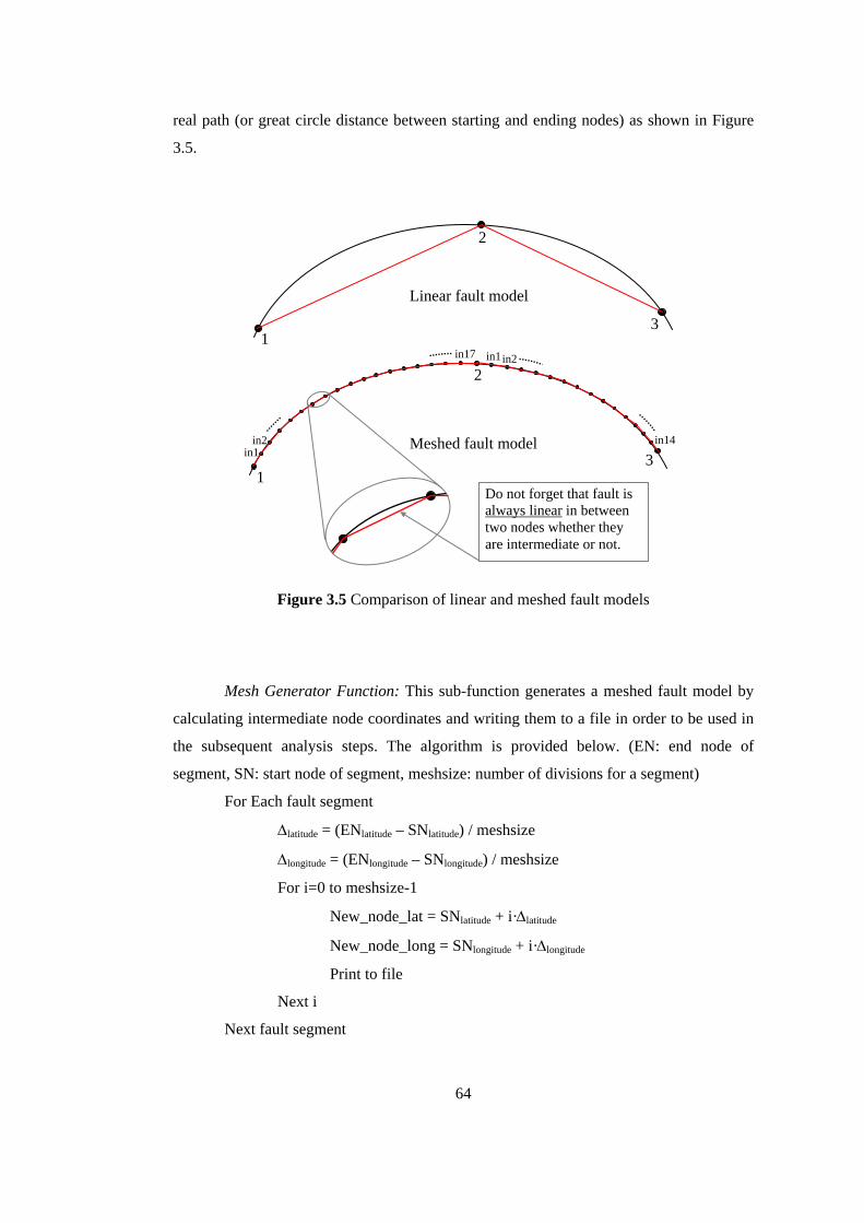
real path (or great circle distance between starting and ending nodes) as shown in Figure

3.5.

Figure 3.5 Comparison of linear and meshed fault models

Mesh Generator Function: This sub-function generates a meshed fault model by

calculating intermediate node coordinates and writing them to a file in order to be used in

the subsequent analysis steps. The algorithm is provided below. (EN: end node of

segment, SN: start node of segment, meshsize: number of divisions for a segment)

For Each fault segment

∆latitude = (ENlatitude – SNlatitude) / meshsize

∆longitude = (ENlongitude – SNlongitude) / meshsize

For i=0 to meshsize-1

New_node_lat = SNlatitude + i·∆latitude

New_node_long = SNlongitude + i·∆longitude

Print to file

Next i

Next fault segment

1

in1

2

3 Meshed fault model

Linear fault model

2

3 1

in17

in2

in1in2

in14

Do not forget that fault is always linear in between two nodes whether they are intermediate or not.

64

Fault characteristics: Every fault model has common properties which are

number of nodes, number of segments, node and segment data matrices. Total number of

nodes and coordinates of each node with its node number are entered manually or read

from a text file. Then program creates segment data matrix automatically. The segment

data matrix includes curved length, linear length and mesh size for each segment. Curved

length is the great circle distance between two end points of the line segment whereas

linear length is the well-known linear distance. Mesh size defines the number of sub-

segments for each segment. Expected moment magnitude of the earthquake is another

fault characteristic. Details of fault model generation are available in the program manual

attached in Appendix - A.

3.2.1.4 Attenuation Relationship Data

Local site conditions have considerable effects on response of buildings under

earthquake loads. This is not only related with the soil type under the site, but it has also

something to do with characteristics of the motion path that seismic waves followed while

reaching the site. Attenuation relationships try to compensate those site effects. SRAS is

capable of handling four different attenuation relationships, which are presented in section

2.3. These attenuation relationships are Gülkan and Kalkan [21], Abrahamson and Silva

[20], Sadigh et al. [16] and Boore et al. [12]. Each attenuation relationship is programmed

as a sub-function and inserted into the main attenuation module. This sub-functioning

makes it handy for further updates and modifications as well as addition of new

attenuation relationships.

The software has an attenuation wizard that enables the user to select the

attenuation model visually. This gives the opportunity to review the limitations of each

relationship and select the most appropriate model for the region under consideration. It is

the users’ responsibility to verify the proper attenuation relationship selection. The wizard

modifies its graphical user interface depending on the selected attenuation relationship to

make the collection of input parameters more straightforward.

3.2.1.5 Analysis Method Data

Analysis method refers to the procedure followed while computing the

displacement demand. The software is capable of handling three well-known procedures.

These are capacity spectrum method, constant ductility method and displacement

65

coefficient method. Each of these methods was discussed in section 2.4 in a detailed

manner.

SRAS takes analysis method as an input which includes some other parameters

related to the selected procedure. ATC-40 procedure requires slice number, error

percentage and structural behavior type of buildings. Slice number and error percentage

are used for the convergence and accuracy of the iterative methodology. Figure 3.6 shows

the definitions for slice number and error percentage. Structural behavior type is selected

for all structures in the inventory as “A”, “B” or “C” which were defined in Table 2.12.

Figure 3.6 Slice number and accuracy

Constant Ductility procedure requires slice number, error percentage and Ry-µ-Tn

relationship. Slice number and error percentage are same as in the case of ATC-40

procedure (Figure 3.6). Ry-µ-Tn relationship is selected from the available three relations,

named as “Newmark – Hall”, “Krawinkler - Nassar” and “Vidic – Fajhar – Fischinger”.

Details of these relations were covered in section 2.4.3. Displacement coefficient method

does not require any parameters since it is not an iterative procedure.

After selecting one of the available procedures using “Analysis Method Wizard”,

an analysis method file is created in order to be used in the analysis. The file may also be

utilized for other analysis since it does not include project or scenario specific parameters.

Details of analysis method file generation are available in the program manual presented

in Appendix - A.

66

3.2.2 Calculation Components

SRAS uses three calculation components. These components are demand

calculation, performance calculation and damage estimation. Initially, demand calculation

module runs and computes the closest distance between each building and fault rupture as

well as spectral acceleration values required to construct a demand curve. Secondly,

performance calculation module starts analysis and computes the demand displacement

for each building. Finally, damage estimation module predicts damage level of each

building. Each of these modules is composed of several sub-routines and functions. The

following paragraphs give details of each component.

3.2.2.1 Demand Calculation

It is the key component of SRAS that is utilizing the attenuation relationships to

generate spectral acceleration curves and attached to the main code as a separate module.

This module is composed of functions that calculate the closest distance to the fault,

compute the spectral acceleration values for each attenuation relationship defined in

section 2.3 and generate demand spectrum.

By using the spatial coordinates of buildings and scenario fault model, the closest

distance between each building and fault is computed which is, in fact, nothing but the

distance of a point to a line segment. This topic is covered in section 2.2. Then, required

parameters for the attenuation relationships become complete. Depending on the selected

attenuation relationship, the spectral acceleration values that are PGA, Sa at T=0.3 sec and

Sa at T=1.0 sec are calculated. Finally, demand calculation module generates a smooth

design-like response curve to be used in the subsequent steps of the analysis. Increasing

fraction of the spectrum is not modeled and it is taken as constant within the interval 0 < T

< Tintersect. This simplifying assumption makes it easier to develop an algorithm for finding

the intersection point of capacity and demand spectra. The programming algorithm is

summarized in the following steps.

1. Calculate the closest distance to the fault

2. Check which site classification scheme is selected (NEHRP [27] / TEC [28]).

3. Check which attenuation relationship is utilized.

4. Interpret the selected site class on the basis of classification scheme and

attenuation relationship. If Boore et al. [12] or Gülkan & Kalkan [21] attenuation

relation is selected, use average shear wave velocity for the selected site class to

67

obtain acceleration response spectrum. For the other two attenuation models use

“Rock” if average shear wave velocity is greater than 550 m/s and use “Soil/Deep

Soil” if average Vs is less than 550 m/s in order to obtain acceleration response

spectrum.

5. Take Sa values at T=0.3 sec and T=1.0 sec as Ia and Iv respectively and construct

simplified acceleration response curve as shown in Figure 3.7. Use this curve as

demand curve in the following steps of analysis.

Sa (g) 5 % damped elastic spectrum

Sa = Iv / T Ia

Figure 3.7 Simplified acceleration response spectrum

3.2.2.2 Performance Calculation

Performance of each building is computed by this module. SRAS is capable of

computing the demand displacement using three different methodologies. These well-

known analysis methods were discussed in section 2.4 including all necessary details.

While developing the software, no additional assumptions were made in addition to the

ones inherited in the methodologies. SRAS is a tool just to perform analyses faster. It does

not recommend new methods or techniques. Considering this aspect, the computed

demand displacements are not more reliable than the method chosen for analysis.

SRAS uses the selected analysis method, which was initially provided as an input,

to calculate demand displacement. Each analysis method is developed as a separate

function within performance calculation module. Each function takes necessary demand

T (s)

Iv

0.3 1.0 Tintersect

68

and capacity parameters and yields performance point. Performance point is a term used to

represent demand displacement. Computed performance point is returned to the main

program as a matrix which has the values of spectral displacement, spectral acceleration

and period. If the performance point can not be found, function returns “-1” for those

values. This is observed when ATC-40 [8] or Constant Ductility [22] procedure was

selected and no intersection is found between capacity curve and reduced demand curve.

In this case, the structure may probably collapse, since demand is much higher than the

available capacity.

3.2.2.3 Damage Estimation

SRAS utilizes two methods for performing damage estimation. The first method is

based on Sd limits (referred as SDL Method from now on) whereas the second method

utilizes damage curves (referred as DC Method from now on). SRAS has default

definitions for both methods and the user may modify the limits or curves depending on

the available building inventory information.

SDL Method: SDL method uses capacity curve in ADRS format to define damage

level intervals. The user may define maximum 9 damage levels and label them

accordingly for each building type. An example is shown in Figure 3.8 for a building type

having three damage levels labeled as “Light”, “Moderate” and “Heavy”. Every building

type has its own damage level definition which means different damage level definitions

can be done for different building types. For instance, if “STEEL” frame structures have

three damage levels, it is possible to assign two or five damage levels to “RC” frame

structures. It is also possible to employ same damage levels for all building types.

The damage level definition process mostly depends on the building types and the

project requirements. While estimating damage, the procedure below is repeated for each

building in the stock.

1. Read type of building and number of stories from the input file and select

appropriate capacity curve for the building.

2. Using damage level definitions, calculate numerical limits for each

damage level interval.

3. Check which interval contains performance point and select that damage

level as estimated building damage.

69

Figure 3.8 Damage estimation based on Sd limits

DC Method: DC method uses damage curves to define percentage damage. For

each building type, the user may define damage curves representing an interval of number

of stories. An example is shown in Figure 3.9 for a building type having three damage

curves representing different intervals of number of stories. Every building type has its

own damage curves, indicating that different intervals of number of stories can be used for

different building types. For instance, if “STEEL” frame structures have three damage

curves, it is possible to assign two or five damage curves to “RC” frame structures. And it

is also possible to employ same number of damage curves for all building types. This is

the case when all type of buildings are classified as “Low-rise (1-3)”, “Mid-rise (4-7)” and

“High-rise (8+)”

In general, the percentage damage estimation may be utilized to obtain smooth

transitions and variations between buildings. While estimating damage, the procedure

below is repeated for each building in the stock.

1. Read type of building and number of stories from the input file and select

appropriate damage curve for the building.

2. Using selected damage curve, read or linearly interpolate percentage

damage value corresponding to the performance point spectral

displacement.

3. Assign that percentage damage to estimate building damage.

70

Figure 3.9 Damage estimation based on damage curves

3.2.3 Output Components

Every program has a special way of displaying or presenting the results. This is

expected since each program is developed for an individual purpose. Output components

refer to sub-routines and graphical interfaces used for conveying results to the user. The

most widespread output components are screen display, report generation and data

storage.

Since the ultimate objective in this study is to develop a user friendly seismic risk

analysis software, tabular results are preferably better than other formats. Almost all well-

known GIS applications, such as ArcGIS and MapInfo, make use of tabular data while

generating maps or geo-databases. Considering this aspect, SRAS is developed to present

the results in both tabular and text file format. The following paragraphs provide detailed

information about each component.

3.2.3.1 Screen Display

Screen display is very practical to check the results for obvious inconsistencies

and critical deviations. If the results are found to be unsatisfactory, then the analysis is

repeated by eliminating the errors in input data until the abnormality disappears. SRAS

presents the results in a table where computed values are appended next to the columns of

building input data. Thus, the number of columns on the output table becomes twenty five.

71

These columns are “Site ID”, “Site Label”, “Building Label”, “Latitude”, “Longitude”,

“Site Class”, “Number of Stories”, “Building Type”, “Number of Buildings”,

“Construction Year”, “Apparent Condition”, “Information”, “Closest Distance (m)”,

“PGA(g)”, “Sa (g) at T = 0.3 s”, “Sa (g) at T = 1 s”, “Tintersect (sec)”, “Say (g)”, “Sdy (cm)”,

“Samax (g)”, “Sdmax (cm)”, “ppSd (cm)”, “ppSa (g)”, “ppT (sec)” and “Damage”. Figure 3.10

shows a screenshot taken from SRAS to present the aforementioned tabular format.

Figure 3.10 SRAS screenshot showing results (only 7 columns are visible)

3.2.3.2 Report Generation

Generally, the results do not mean much unless the methodology followed is

verified. So, not only the results but also the methodology should be presented in an

72

appropriate way. Engineering reports are the best ways of conveying the outcome of a

study to the authorities concerned. Regarding to this aspect, SRAS is equipped with a

report generation module. This module prepares a preliminary report for the project

including input data, methodology and results.

The report is composed of several pages. There is a cover page showing the

project title, information about the person who made the study and report generation date

and time. Secondly, building inventory statistics are given instead of writing all building

data. Then, nodal and segmental data of the scenario earthquake fault model is added to

the report. Next, attenuation relationship, analysis method and capacity curve data are

provided. Finally, the estimated damage distribution within the district for each building

type is printed and report generation is finalized. Details of report generation process are

explained in program manuals that are provided in Appendix - A.

3.2.3.3 Exporting Results as Database File

After completing initial screening of the results, it is necessary to export results.

The results are exported as database files since tabulated results will ease post-processing.

Two database formats are supported by SRAS. These are Microsoft Excel Worksheet

(*.xls) and Access Database (*.mdb). While generating digital maps or geodatabases,

these file formats are quite handy and practical. The created output file includes all data

shown on screen as aforementioned in section 3.2.3.1. No additional information is given

regarding to the methodology used. Details for exporting results are available in program

manuals appended as Appendix - A.

73

CHAPTER 4

VERIFICATION OF SRAS

4.1 INTRODUCTION

Every computer program should be checked for the inconsistencies and errors

after development process. This phase is called as debugging. The best way of software

debugging is to use it for benchmark problems and compare the outputs with benchmark

results. If the results are same or very similar, the software proves to be reliable. But in the

case of risk analysis and damage distribution, the situation is not that simple. Observed

regional damage distribution reported after an earthquake may show significant variations

depending on the selected assessment methodology and even on the assessment team

employed. For instance, two separate teams may present different damage distribution

maps that follow the same trend but have dissimilar quantitative results for the same

region. So, this makes it quite difficult to define a quantitative benchmark case in risk

analysis problems. Since no quantitative benchmark results are available, the best thing to

do is trying to catch the general trend in regional damage distribution and to predict the

number of collapsed buildings satisfactorily for the region experiencing an earthquake. By

means of spot checks of intermediate steps, the modules of the software can be debugged

as well.

SRAS has been verified by using it for the estimation of damage distribution in

Adapazari due to August 17, 1999 Izmit Earthquake. Although it is known prior to the

verification that the damage pattern in Adapazari was too multifaceted to be predicted by

conventional regional assessment procedures, it is aimed to check SRAS outcome for the

consistency of results rather than the precise correspondence with the observed damage

statistics by General Directorate of Disaster Affairs (GDDA). The verification process will

74

be explained in four sections. First section describes the input parameters used in the

analysis. Second part gives details of damage estimation methodology. Third section

presents the results and the last part discusses reliability of the results as well as SRAS.

4.2 INPUT PARAMETERS

Adapazari district and fault rupture generated by the August 17, 1999 Izmit

Earthquake are mapped and presented in Figure 4.1. Required input parameters for the

assessment are building inventory data, scenario earthquake fault data, attenuation

relationship data, capacity curve data and analysis method data. These input parameters

will be explained in the following paragraphs to demonstrate clearly what was provided to

SRAS as input. Since building inventory database is quite large, it will be a vain attempt

to present all buildings as tables. Instead, only statistical information is provided here

regarding to the building inventory. Data files are appended to the attached disk.

Figure 4.1 Adapazari and August 17, 1999 Izmit Earthquake fault rupture location

75

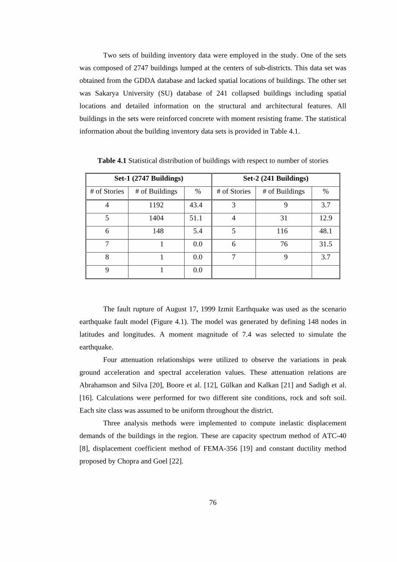
Two sets of building inventory data were employed in the study. One of the sets

was composed of 2747 buildings lumped at the centers of sub-districts. This data set was

obtained from the GDDA database and lacked spatial locations of buildings. The other set

was Sakarya University (SU) database of 241 collapsed buildings including spatial

locations and detailed information on the structural and architectural features. All

buildings in the sets were reinforced concrete with moment resisting frame. The statistical

information about the building inventory data sets is provided in Table 4.1.

Table 4.1 Statistical distribution of buildings with respect to number of stories

Set-1 (2747 Buildings) Set-2 (241 Buildings)

# of Stories # of Buildings % # of Stories # of Buildings %

4 1192 43.4 3 9 3.7

5 1404 51.1 4 31 12.9

6 148 5.4 5 116 48.1

7 1 0.0 6 76 31.5

8 1 0.0 7 9 3.7

9 1 0.0

The fault rupture of August 17, 1999 Izmit Earthquake was used as the scenario

earthquake fault model (Figure 4.1). The model was generated by defining 148 nodes in

latitudes and longitudes. A moment magnitude of 7.4 was selected to simulate the

earthquake.

Four attenuation relationships were utilized to observe the variations in peak

ground acceleration and spectral acceleration values. These attenuation relations are

Abrahamson and Silva [20], Boore et al. [12], Gülkan and Kalkan [21] and Sadigh et al.

[16]. Calculations were performed for two different site conditions, rock and soft soil.

Each site class was assumed to be uniform throughout the district.

Three analysis methods were implemented to compute inelastic displacement

demands of the buildings in the region. These are capacity spectrum method of ATC-40

[8], displacement coefficient method of FEMA-356 [19] and constant ductility method

proposed by Chopra and Goel [22].

76

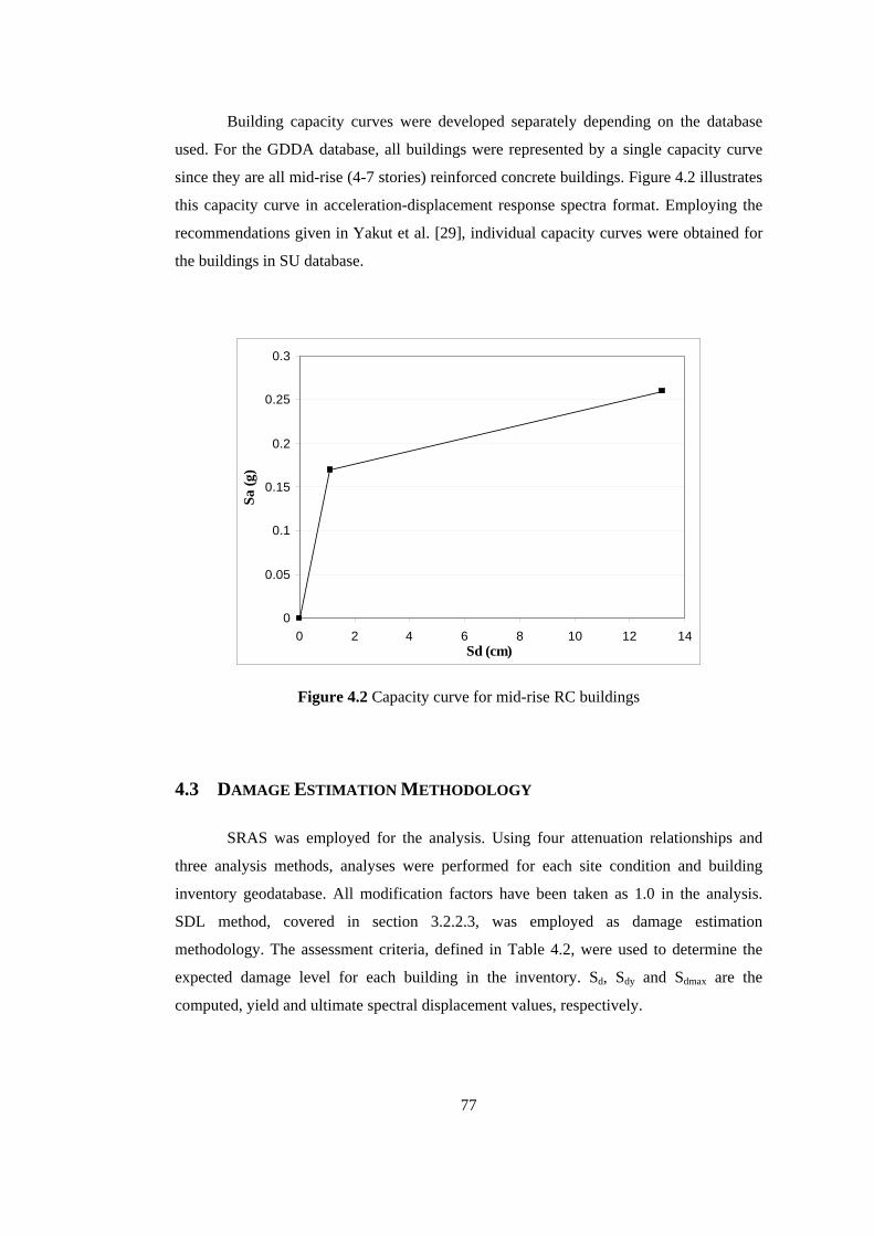
Building capacity curves were developed separately depending on the database

used. For the GDDA database, all buildings were represented by a single capacity curve

since they are all mid-rise (4-7 stories) reinforced concrete buildings. Figure 4.2 illustrates

this capacity curve in acceleration-displacement response spectra format. Employing the

recommendations given in Yakut et al. [29], individual capacity curves were obtained for

the buildings in SU database.

0

0.05

0.1

0.15

0.2

0.25

0.3

0 2 4 6 8 10 12 1Sd (cm)

Sa (g

)

4

Figure 4.2 Capacity curve for mid-rise RC buildings

4.3 DAMAGE ESTIMATION METHODOLOGY

SRAS was employed for the analysis. Using four attenuation relationships and

three analysis methods, analyses were performed for each site condition and building

inventory geodatabase. All modification factors have been taken as 1.0 in the analysis.

SDL method, covered in section 3.2.2.3, was employed as damage estimation

methodology. The assessment criteria, defined in Table 4.2, were used to determine the

expected damage level for each building in the inventory. Sd, Sdy and Sdmax are the

computed, yield and ultimate spectral displacement values, respectively.

77

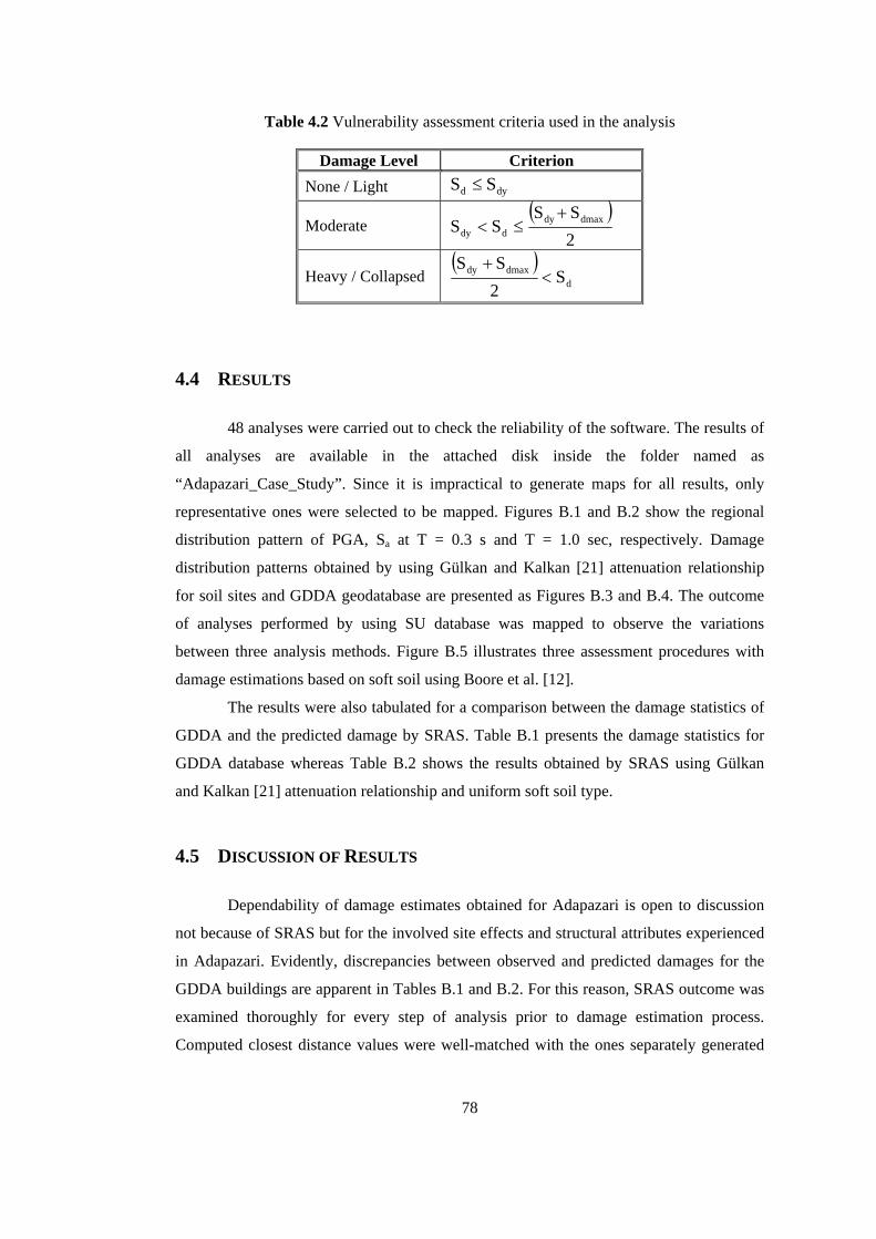
Table 4.2 Vulnerability assessment criteria used in the analysis

Damage Level Criterion None / Light dyd SS ≤

Moderate ( )

2SS

SS dmaxdyddy

+≤<

Heavy / Collapsed ( )

ddmaxdy S

2SS

<+

4.4 RESULTS

48 analyses were carried out to check the reliability of the software. The results of

all analyses are available in the attached disk inside the folder named as

“Adapazari_Case_Study”. Since it is impractical to generate maps for all results, only

representative ones were selected to be mapped. Figures B.1 and B.2 show the regional

distribution pattern of PGA, Sa at T = 0.3 s and T = 1.0 sec, respectively. Damage

distribution patterns obtained by using Gülkan and Kalkan [21] attenuation relationship

for soil sites and GDDA geodatabase are presented as Figures B.3 and B.4. The outcome

of analyses performed by using SU database was mapped to observe the variations

between three analysis methods. Figure B.5 illustrates three assessment procedures with

damage estimations based on soft soil using Boore et al. [12].

The results were also tabulated for a comparison between the damage statistics of

GDDA and the predicted damage by SRAS. Table B.1 presents the damage statistics for

GDDA database whereas Table B.2 shows the results obtained by SRAS using Gülkan

and Kalkan [21] attenuation relationship and uniform soft soil type.

4.5 DISCUSSION OF RESULTS

Dependability of damage estimates obtained for Adapazari is open to discussion

not because of SRAS but for the involved site effects and structural attributes experienced

in Adapazari. Evidently, discrepancies between observed and predicted damages for the

GDDA buildings are apparent in Tables B.1 and B.2. For this reason, SRAS outcome was

examined thoroughly for every step of analysis prior to damage estimation process.

Computed closest distance values were well-matched with the ones separately generated

78

using the commercial software ArcView 8.3. Thus, distance calculation module proves its

reliability. Calculated demand parameters were also verified by manual execution of

attenuation relationship equations. Unsurprisingly, PGA and Sa values were decreasing as

getting away from the fault. So, demand calculation module proves to be consistent and

dependable. Computed inelastic displacement demands were compared with the ones

calculated separately by hand and they were almost same ignoring insignificant rounding

errors. Finally, damage estimation module was checked for its dependability. This was the

easiest part because even rapid screening of results was sufficient to justify damage level

assignments made by SRAS. In summary, SRAS has proved to be a reliable tool for

performing lengthy calculations of conventional regional assessment procedures.

79

CHAPTER 5

CASE STUDY: ISTANBUL

5.1 INTRODUCTION

The 17 August 1999 Mw = 7.4 Izmit and 12 November 1999 Mw = 7.1 Düzce

earthquakes prompted seismologists and geologists to conduct studies to predict

magnitude and location of a potential earthquake that can cause substantial damage in

Istanbul. One of these studies was Parsons et al. [31] and the striking outcome of the study

was summarized as follows: (Parsons et al. [31])

We find a 62±15% probability of strong shaking (MMI~>VIII;

equivalent to a peak ground acceleration of 0.34-0.65g (Wald et al., 1999) in greater Istanbul over the next 30 yr (May 2000-2030), 50±13% over the next 22 yr, and 32±12% over the next 10 yr. Inclusion of renewal doubles the time-averaged probability; interaction further increases the probability by a factor of 1.3.

These extremely high probabilities of occurrence have triggered responsible

authorities to take precautions to reduce the casualties and the losses from the expected

earthquake. Among several studies carried out, as discussed previously, JICA has

performed an extensive study (referred as JICA Study [11] from now on) that covers a

large study area and building inventory (referred as JICA database from now on). All data

including building inventory, scenario faults, site classes, damage estimation results etc.

were made public for researchers. As an application of the software developed in this

study, it was intended to re-calculate the probable damage distribution in Istanbul using

the JICA database by employing newly developed capacity curves that are peculiar to

construction practice in Turkey.

80

Considering this aspect, SRAS has been utilized for the estimation of probable

damage distribution in Istanbul due to a scenario earthquake (model A of JICA Study

[11]) of moment magnitude 7.5. Three separate analyses were performed to be able to

make comparisons. These analyses will be referred as JICA-Check, JICA-New, and IMM-

New.

All data used for the analyses were recorded to the attached disk as a zipped folder

named as “Istanbul_Case_Study”. A “Read Me” file was put into the same folder to

explain directory mapping. The interested reader may perform several analyses; prepare

maps or tables of interest by using the available data on the attached disk. Each analysis

carried out in this study is explained separately in Section 5.2. The results obtained from

the analyses are compared and discussed in Section 5.3.

5.2 DAMAGE ESTIMATION FOR ISTANBUL

Three analyses, namely JICA-Check, JICA-New and IMM-New, were carried out.

The similarities and differences between the analyses are presented in the following table.

Table 5.1 Comparison of analyses performed for estimating damage in Istanbul

JICA-Check JICA-New IMM-New

Building

Inventory

The ratios for building

types and heights in

JICA database were

converted to number of

buildings. This rough

conversion inherits

certain assumptions.

The building inventory

obtained from IMM was

intersected with the

JICA Study area and

those falling within the

study area were selected

for the analysis.

The building

inventory obtained

from IMM was used.

Site

Classification

Map

Site classification map

proposed in JICA Study

was utilized to assign

the site classes.

Site classification map

proposed in JICA Study

was utilized to assign the

site classes.

A new site

classification map

was utilized.

Capacity

Curves

Newly developed

capacity curves were

used.

Newly developed

capacity curves were

used.

Newly developed

capacity curves were

used.

81

Although results of regional damage estimation process require lots of maps and

tables, in this study it is believed to be more effective to display representative maps and

tabulate damage estimation results in district level. For this purpose, maps and tables,

presented in Table 5.2, were prepared for each analysis.

Table 5.2 Selected maps and tables to be presented for each analysis

MAPS TABLES

JICA-Check

Ground Classification (JICA)

Distribution of PGA

Distribution of Sa at T = 0.3 s

Distribution of Sa at T = 1.0 s

Distribution of Heavily DB*

Distribution of Moderately DB**

Distribution of Lightly DB**

Summary of damage

estimation results in

district level

JICA-New

Distribution of Heavily DB

Distribution of Moderately DB**

Distribution of Lightly DB**

Summary of damage

estimation results in

district level

IMM-New

Ground Classification (New)**

Distribution of PGA**

Distribution of Sa at T = 0.3 s**

Distribution of Sa at T = 1.0 s**

Distribution of Heavily DB

Distribution of Moderately DB**

Distribution of Lightly DB**

Summary of damage

estimation results in

district level

DB*: Damaged Buildings, **: presented in Appendix C

While generating maps for heavily/moderately/lightly damaged buildings, the

ratio of damaged buildings to the total number of buildings for each district was utilized

since these ratios provide valuable information for the comparison between different

analyses. Number of damaged buildings in the districts of a province may show drastic

variations whereas the ratios show gradual changes. In view of this, the ratios were

employed while generating damage distribution maps.

82

As a technical reminder, building inventory database for Istanbul was extremely

large and each analysis took almost an hour using a Pentium-4 computer having 1 GHz

RAM. It would probably take longer time on another computer depending on the memory

and processor units. Although the processing time seems quite long, it is comparable to

other GIS based damage estimation programs that perform analysis on the basis of

buildings rather than grids. Using grids decreases the processing time but causes loss of

accuracy.

In the subsequent sections 5.2.1, 5.2.2 and 5.2.3, the analyses are explained under

three subtitles: Input data, Analysis and Results. Each part was made as concise as

possible to prevent any confusions or misinterpretations. The input parameters used in the

analysis were described in input data part. Analysis part gives details of damage

estimation methodology and the last part presents the results. An overall comparison for

these analyses and the other studies is provided in section 5.3.

5.2.1 JICA-Check

Input data: Required input parameters for the assessment are building inventory

data, scenario earthquake fault data, attenuation relationship data, capacity curve data and

analysis method data.

Building inventory data set (JICA database) was composed of 724,561 buildings

lumped at the centers of 0.005˚ by 0.005˚ grids. This data set was obtained from the JICA

Study [11] and converted into a new format in order to make it ready for use in SRAS.

The original data set (JICA database) contained the number of buildings and their

corresponding ratios defined for each building type, building height and the construction

year. Unfortunately, no additional information was available to show a relationship

between the ratios provided for different characteristics. It was almost impossible to

calculate the number of buildings for a specified building type, height and construction

year. Due to these limitations it was assumed that the percentage of each building type for

a district is also valid for the distribution within each building height interval. This

assumption has eliminated the difficulty in relating building type to building height. The

construction year could not be used due to lack of reliable data. Converted building

inventory data were overlaid on ground classification map of JICA Study [11] and

associated NEHRP site classes were obtained for each building group lumped at the

centers of grids. Building inventory summary based on building type is shown in Table

5.3.

83

Table 5.3 Building type statistics for JICA-Check

Building Type Number of Buildings Percentage (%)

RC 545,697 75.31 WOOD 10,944 1.51 MASONRY 165,249 22.81 RC Shear Wall 761 0.11 PREFABRIC 873 0.12 STEEL 1,037 0.14

Total 724,561 100.00

Scenario earthquake fault model A, proposed in the JICA Study [11], was

employed for the analysis. This model was the most probable model and the assigned

moment magnitude was 7.5. Attenuation relationship of Boore et al. [12] was utilized

since it was also selected to be used in the JICA Study [11].

Capacity curves for reinforced concrete frame structures were obtained from

Yakut et al. [29]. These curves were scaled with the relativity coefficients to generate

capacity curves for other building types. These coefficients are obtained from the ratio of

capacity curve values (proposed in HAZUS) for reinforced concrete structures to the

values for other building types. Thus, capacity curves for each building type were

produced and they are peculiar to the practice in Turkey. Capacity spectrum method of

ATC-40 [8] was selected for the computation of demand displacements.

Analysis: Using the input data mentioned above, the analysis was carried out to

estimate damage level of each building. The SDL method was used in damage estimation.

Three damage levels were introduced as “Lightly damaged”, “Moderately damaged” and

“Heavily damaged”. Another damage level, labeled as “Collapse/No Intersection”, was

created automatically by SRAS for those buildings having no intersection between their

capacity and demand curves. They were added to the “Heavily damaged” building class.

The damage level limits used in the study are given in Table 5.4.

84

Table 5.4 Damage level limits defined for JICA-Check

Damage Level Criterion Light dyd SS ≤

Moderate ( )

2SS

SS dmaxdyddy

+≤<

Heavy / Collapsed ( )

ddmaxdy S

2SS

<+

Results: The results including all data files and ArcView 8.3 map files are

available in the attached disk inside the folder named as “JICA-Check”. Since it is

impractical to generate maps for all results, only representative ones were selected to be

mapped. Figure 5.1 demonstrates ground classification map used by JICA Study [11].

Figures 5.2, 5.3 and 5.4 show the regional distribution patterns of PGA, Sa at T = 0.3 s and

T = 1.0 sec, respectively. Maps for the distribution of lightly, moderately and heavily

damaged buildings are given in Figures C.2, C.3 and 5.5, respectively.

The results were also tabulated for a comparison between the three analyses and

previous studies. Table 5.7 presents the damage estimation results for Istanbul obtained by

SRAS using Boore et al. [12] attenuation relationship.

5.2.2 JICA-New

Input data: Required input parameters for the assessment are building inventory

data, scenario earthquake fault data, attenuation relationship data, capacity curve data and

analysis method data. Scenario earthquake fault model, attenuation relationship, capacity

curves and analysis method were selected the same as the ones used in the JICA-Check.

Building inventory data set (IMM database) was composed of 1,409,487 buildings

having their spatial coordinates. This data set was obtained from the IMM and projected

into a new coordinate system in order to obtain the coordinates in latitudes and longitudes.

Then by using ArcView 8.3, these buildings were overlaid on ground classification map of

JICA Study [11] and associated NEHRP site classes were obtained for the ones falling in

the study area of JICA. The buildings lacking ground class information were removed

from the database. Based on building type and number of stories, a second elimination

was performed to delete buildings missing that information. Finally, 1,195,711 buildings

were made ready for the use in SRAS. Unfortunately, no additional information was

85

available regarding to the construction years and apparent conditions of the buildings.

Building inventory summary based on building type is shown in Table 5.5.

Table 5.5 Building type statistics for JICA-New

Building Type Number of Buildings Percentage (%)

RC 1,038,641 86.86 MASONRY 144,214 12.06 STEEL 904 0.08 WOOD 6,486 0.54 TUNNEL 2 0.00 OTHERS 5,461 0.46 PREFABRIC 3 0.00

Total 1,195,711 100.00

Analysis: Using the input data mentioned above, the analysis was carried out to

estimate damage level of each building. The SDL method was used in damage estimation.

The damage levels and limits that were introduced in the JICA-Check part were also

utilized while performing analysis for this part.

Results: The results including all data files and ArcView 8.3 map files are

available in the attached disk inside the folder named as “JICA-New”. Only representative

results were selected to be mapped. Since ground classification map of JICA Study [11]

was used, distribution of PGA and spectral acceleration values will be the same with those

maps (Figures 5.1, 5.2, 5.3 and 5.4) presented for JICA-Check part. The maps for the

distribution of lightly, moderately and heavily damaged buildings are given in Figures

C.4, C.5 and 5.6, respectively.

The results were also tabulated for a comparison between the three analyses and

previous studies. Table 5.8 presents the damage estimation results for Istanbul obtained by

SRAS using Boore et al. [12] attenuation relationship.

5.2.3 IMM-New

Input data: Required input parameters for the assessment are building inventory

data, scenario earthquake fault data, attenuation relationship data, capacity curve data and

analysis method data.

86

Similar to the case JICA-New IMM database was used. By using ArcView 8.3,

these buildings were overlaid on ground classification map proposed in this study and

associated NEHRP site classes were obtained for the ones falling in the ground

classification map area. The buildings lacking ground class information were removed

from the database. Based on building type and number of stories, a second elimination

was performed to delete buildings missing that information. Finally, 1,313,327 buildings

were made ready for the use in SRAS. Unfortunately, no additional information was

available regarding to construction years and apparent conditions of the buildings.

Building inventory summary based on building type is shown in Table 5.6. Scenario

earthquake fault model, attenuation relationship, capacity curves and analysis method

were selected as the ones used in the JICA-Check.

Table 5.6 Building type statistics for IMM-New

Building Type Number of Buildings Percentage (%) RC 1,140,695 86.86 MASONRY 159,523 12.15 STEEL 907 0.07 WOOD 6,728 0.51 TUNNEL 2 0.00 OTHERS 5,469 0.42 PREFABRIC 3 0.00

Total 1,313,327 100.00

Analysis: Using the input data mentioned above, the analysis was carried out to

estimate damage level of each building. The SDL method was used in damage estimation.

The damage levels and limits that were introduced in the JICA-Check part were also

utilized for this part.

Results: The results including all data files and ArcView 8.3 map files are

available in the attached disk inside the folder named as “IMM-New”. Figure C.6

demonstrates ground classification map proposed by this study. Figures C.7, C.8 and C.9

show the regional distribution patterns of PGA, Sa at T = 0.3 s and T = 1.0 s, respectively.

Maps for the distribution of lightly, moderately and heavily damaged buildings are given

in Figures C.10, C.11 and 5.7, respectively. An additional map showing all damage levels

at once was also provided as Figure C.12.

87

The results were tabulated for a comparison between the three analyses and

previous studies. Table 5.9 presents the damage estimation results for Istanbul obtained by

SRAS using Boore et al. [12] attenuation relationship.

5.3 DISCUSSION OF RESULTS

Damage estimates obtained for Istanbul using different building inventories and

ground classification maps prove once again that reliability of regional damage estimation

strongly depends on the quality and accuracy of the data at hand. Discrepancies between

the results of three analyses and JICA Study [11] were expected since all of them have

special deficiencies in different steps of the process. For instance, JICA Study [11] uses

capacity curves that do not reflect the real practice in Turkey. JICA-Check database is not

so dependable since it inherits considerable assumptions. JICA-New employs ground

classification map proposed by JICA. IMM-New utilizes a new but rough ground

classification map that is generated from surface geology maps of Istanbul. So, it should

be better to discuss the effects of each parameter; building inventory, ground classification

map and capacity curve, separately.

Two databases: JICA and IMM differ significantly in the number of buildings that

they contain. The number of buildings in the IMM database almost doubles the number of

buildings in the JICA database. The IMM database seems more reliable than JICA

database considering the information about number of stories, but it may be misleading for

building type information. On the other hand JICA database is a secret box that shields

what is inside. In view of these, building inventory effect can not be investigated in a

detailed manner with the available databases. Assumptions made in JICA-Check part

while trying to extract building inventory data gave rise to unrealistic results. As can be

easily observed from Tables 5.7, JICA-Check predicted no heavily damaged buildings for

the districts: Besiktas, Beykoz, Gaziosmanpasa, Kagithane, Sariyer, Sisli, Tuzla and

Uskudar. This mainly results from high percentage of low-rise buildings for those

districts. Although it is not common to have high-rise masonry or wood buildings, JICA-

Check database contains many of those unrealistic buildings coming from conversion of

the ratios to number of buildings depending on the percentage of building type. So, the

districts having high percentages of high and mid-rise buildings had high percentages of

heavily damaged buildings since most of them came out to be masonry. But JICA-Check

88

was just a preliminary study in order to find and debug errors in SRAS prior to the IMM-

New part.

Ground classification map affects the results significantly. The maps of JICA and

this study basically differ for the European side of Istanbul. There are minor differences

for the Anatolian side. Besides this, there are some districts such as Zeytinburnu where

two maps hold opposing views. JICA map proposes NEHRP site class “D” for

Zeytinburnu whereas NEHRP site class “B” was proposed by the new map. Districts

should be divided into two in order to figure out the effects of site class variation. First

group districts are those that are fully or partially assigned to stiffer ground classes in the

new map. These districts are Avcilar, Bagcilar, Bahcelievler, Bakirkoy, Bayrampasa,

Besiktas, Beyoglu, Eminonu, Esenler, Eyup, Fatih, Gungoren, Kagithane, Kucukcekmece

and Zeytinburnu. For these districts, the IMM-New results for heavily damaged building

ratios are lower than the ones calculated in JICA-New. Second group districts are those

that are fully or partially assigned to softer ground classes in the new map. These districts

are Adalar, Beykoz, Gaziosmanpasa, Kadikoy, Kartal, Maltepe, Pendik, Sariyer, Sisli,

Tuzla, Umraniye and Uskudar. For these districts, the IMM-New results for heavily

damaged building ratios are higher than the ones calculated in JICA-New. Therefore, site

effects verify their importance in damage estimation process.

Capacity curves were the most critical part of the analysis. A sample group of

capacity curves for reinforced concrete frame structures used by JICA and this study is

presented in Figure C.1. As can be directly observed from Figure C.1, the capacity curves

used in this study have lower capacity but higher ductility as compared to the ones used by

JICA. This is responsible for the high percentages of moderately and heavily damaged

buildings. Because when yield capacity is low and ductility is high, demand spectrum

generally intersects with the capacity spectrum between the yield and ultimate capacity

points.

In summary, the results obtained from the analyses and the JICA results do require

further detailed investigation in order to discover the shielded factors affecting results.

Although there are some discrepancies, the results of IMM-New and JICA seem to be

quite compatible. Supplementary analyses may be carried out easily by using SRAS and

utilizing updated ground classification maps, capacity curves, attenuation relationships

and building inventory data. Since these analyses have been performed as a case study,

broad examination of results is out of the scope of this study. All building input files for

SRAS, maps and ArcView 8.3 files are provided in the attached disk.

89

Figu

re 5

.1 G

roun

d cl

assi

ficat

ion

map

pro

pose

d by

JIC

A S

tudy

[11]

90

Figu

re 5

.2 D

istri

butio

n of

pea

k gr

ound

acc

eler

atio

n (J

ICA

-Che

ck)

91

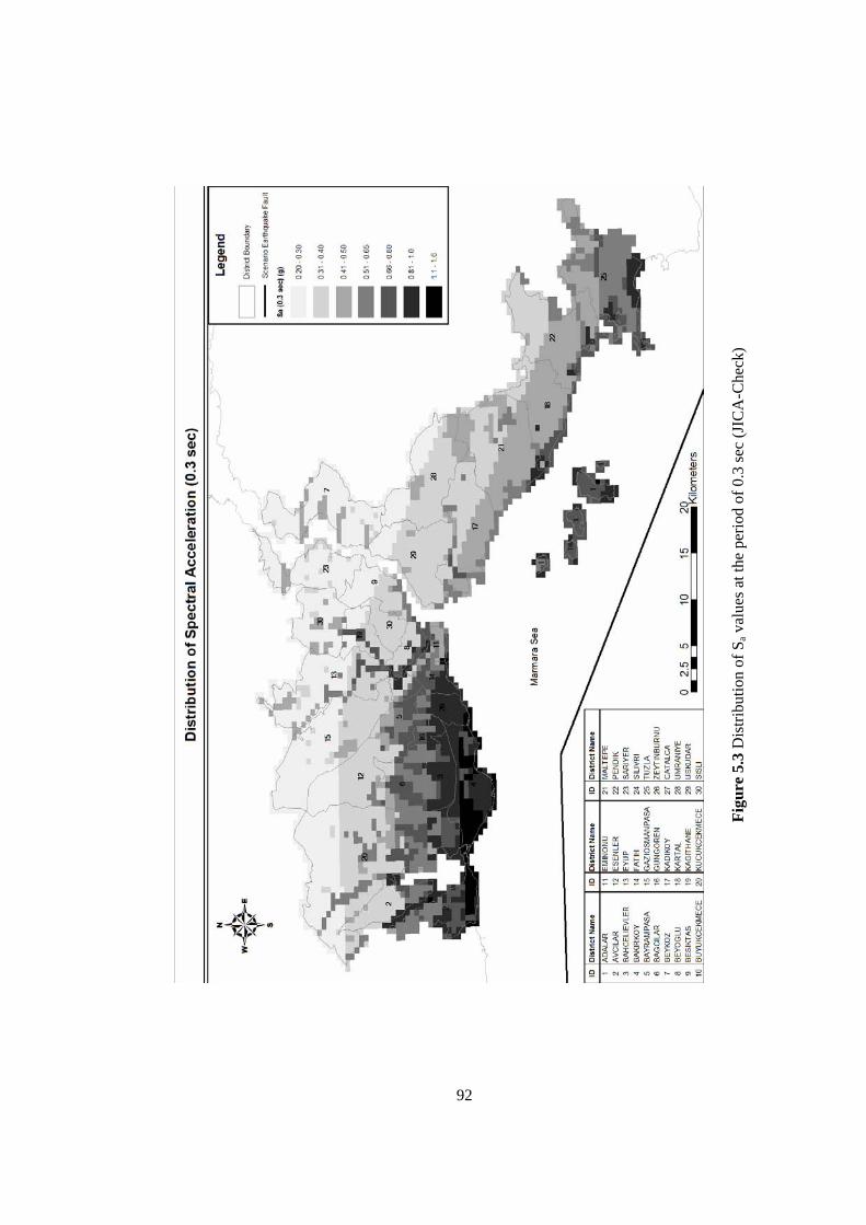
Figu

re 5

.3 D

istri

butio

n of

Sa v

alue

s at t

he p

erio

d of

0.3

sec

(JIC

A-C

heck

)

92

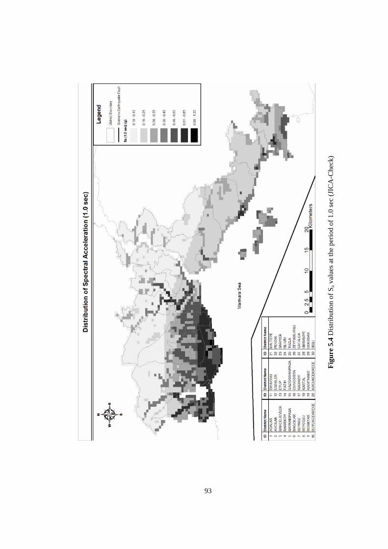
Figu

re 5

.4 D

istri

butio

n of

Sa v

alue

s at t

he p

erio

d of

1.0

sec

(JIC

A-C

heck

)

93

Figu

re 5

.5 D

istri

butio

n of

hea

vily

dam

aged

bui

ldin

gs ra

tio (J

ICA

-Che

ck)

94

Figu

re 5

.6 D

istri

butio

n of

hea

vily

dam

aged

bui

ldin

gs ra

tio (J

ICA

-New

)

95

Figu

re 5

.7 D

istri

butio

n of

hea

vily

dam

aged

bui

ldin

gs ra

tio (I

MM

-New

)

96

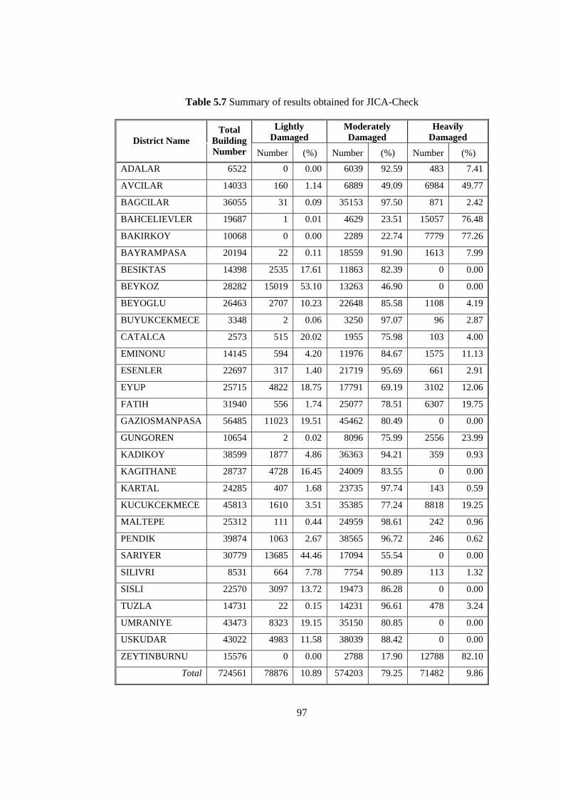
Table 5.7 Summary of results obtained for JICA-Check

Lightly Damaged

Moderately Damaged

Heavily Damaged District Name

Total Building Number Number (%) Number (%) Number (%)

ADALAR 6522 0 0.00 6039 92.59 483 7.41

AVCILAR 14033 160 1.14 6889 49.09 6984 49.77

BAGCILAR 36055 31 0.09 35153 97.50 871 2.42

BAHCELIEVLER 19687 1 0.01 4629 23.51 15057 76.48

BAKIRKOY 10068 0 0.00 2289 22.74 7779 77.26

BAYRAMPASA 20194 22 0.11 18559 91.90 1613 7.99

BESIKTAS 14398 2535 17.61 11863 82.39 0 0.00

BEYKOZ 28282 15019 53.10 13263 46.90 0 0.00

BEYOGLU 26463 2707 10.23 22648 85.58 1108 4.19

BUYUKCEKMECE 3348 2 0.06 3250 97.07 96 2.87

CATALCA 2573 515 20.02 1955 75.98 103 4.00

EMINONU 14145 594 4.20 11976 84.67 1575 11.13

ESENLER 22697 317 1.40 21719 95.69 661 2.91

EYUP 25715 4822 18.75 17791 69.19 3102 12.06

FATIH 31940 556 1.74 25077 78.51 6307 19.75

GAZIOSMANPASA 56485 11023 19.51 45462 80.49 0 0.00

GUNGOREN 10654 2 0.02 8096 75.99 2556 23.99

KADIKOY 38599 1877 4.86 36363 94.21 359 0.93

KAGITHANE 28737 4728 16.45 24009 83.55 0 0.00

KARTAL 24285 407 1.68 23735 97.74 143 0.59

KUCUKCEKMECE 45813 1610 3.51 35385 77.24 8818 19.25

MALTEPE 25312 111 0.44 24959 98.61 242 0.96

PENDIK 39874 1063 2.67 38565 96.72 246 0.62

SARIYER 30779 13685 44.46 17094 55.54 0 0.00

SILIVRI 8531 664 7.78 7754 90.89 113 1.32

SISLI 22570 3097 13.72 19473 86.28 0 0.00

TUZLA 14731 22 0.15 14231 96.61 478 3.24

UMRANIYE 43473 8323 19.15 35150 80.85 0 0.00

USKUDAR 43022 4983 11.58 38039 88.42 0 0.00

ZEYTINBURNU 15576 0 0.00 2788 17.90 12788 82.10

Total 724561 78876 10.89 574203 79.25 71482 9.86

97

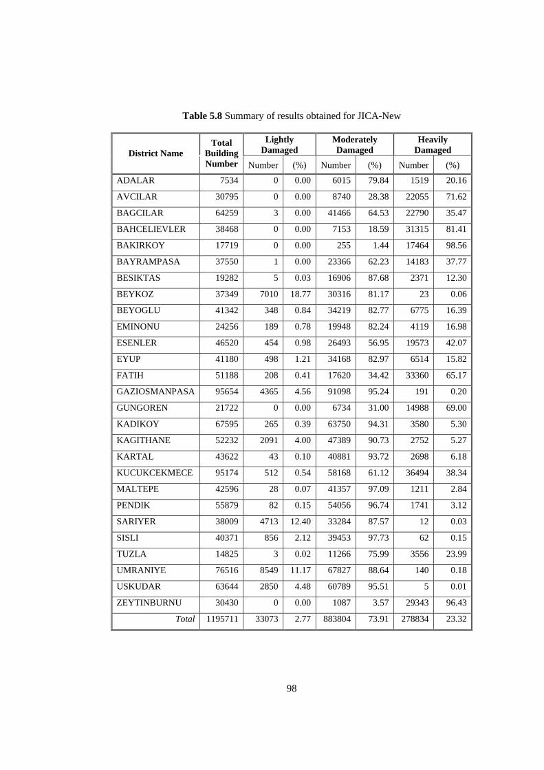
Table 5.8 Summary of results obtained for JICA-New

Lightly Damaged

Moderately Damaged

Heavily Damaged District Name

Total Building Number Number (%) Number (%) Number (%)

ADALAR 7534 0 0.00 6015 79.84 1519 20.16

AVCILAR 30795 0 0.00 8740 28.38 22055 71.62

BAGCILAR 64259 3 0.00 41466 64.53 22790 35.47

BAHCELIEVLER 38468 0 0.00 7153 18.59 31315 81.41

BAKIRKOY 17719 0 0.00 255 1.44 17464 98.56

BAYRAMPASA 37550 1 0.00 23366 62.23 14183 37.77

BESIKTAS 19282 5 0.03 16906 87.68 2371 12.30

BEYKOZ 37349 7010 18.77 30316 81.17 23 0.06

BEYOGLU 41342 348 0.84 34219 82.77 6775 16.39

EMINONU 24256 189 0.78 19948 82.24 4119 16.98

ESENLER 46520 454 0.98 26493 56.95 19573 42.07

EYUP 41180 498 1.21 34168 82.97 6514 15.82

FATIH 51188 208 0.41 17620 34.42 33360 65.17

GAZIOSMANPASA 95654 4365 4.56 91098 95.24 191 0.20

GUNGOREN 21722 0 0.00 6734 31.00 14988 69.00

KADIKOY 67595 265 0.39 63750 94.31 3580 5.30

KAGITHANE 52232 2091 4.00 47389 90.73 2752 5.27

KARTAL 43622 43 0.10 40881 93.72 2698 6.18

KUCUKCEKMECE 95174 512 0.54 58168 61.12 36494 38.34

MALTEPE 42596 28 0.07 41357 97.09 1211 2.84

PENDIK 55879 82 0.15 54056 96.74 1741 3.12

SARIYER 38009 4713 12.40 33284 87.57 12 0.03

SISLI 40371 856 2.12 39453 97.73 62 0.15

TUZLA 14825 3 0.02 11266 75.99 3556 23.99

UMRANIYE 76516 8549 11.17 67827 88.64 140 0.18

USKUDAR 63644 2850 4.48 60789 95.51 5 0.01

ZEYTINBURNU 30430 0 0.00 1087 3.57 29343 96.43

Total 1195711 33073 2.77 883804 73.91 278834 23.32

98

Table 5.9 Summary of results obtained for IMM-New

Lightly Damaged

Moderately Damaged

Heavily Damaged District Name

Total Building Number Number (%) Number (%) Number (%)

ADALAR 7534 0 0.00 5218 69.26 2316 30.74

AVCILAR 30757 0 0.00 12720 41.36 18037 58.64

BAGCILAR 64017 22 0.03 58398 91.22 5597 8.74

BAHCELIEVLER 38596 0 0.00 23769 61.58 14827 38.42

BAKIRKOY 17647 0 0.00 10305 58.40 7342 41.60

BAYRAMPASA 37518 1 0.00 37293 99.40 224 0.60

BESIKTAS 19195 0 0.00 19187 99.96 8 0.04

BEYKOZ 43263 8886 20.54 31452 72.70 2925 6.76

BEYOGLU 41262 0 0.00 37535 90.97 3727 9.03

BUYUKCEKMECE 7513 1 0.01 6708 89.29 804 10.70

EMINONU 24256 0 0.00 23751 97.92 505 2.08

ESENLER 46492 1 0.00 44700 96.15 1791 3.85

EYUP 43526 115 0.26 39023 89.65 4388 10.08

FATIH 51200 93 0.18 47998 93.75 3109 6.07

GAZIOSMANPASA 93580 67 0.07 91932 98.24 1581 1.69

GUNGOREN 21742 2 0.01 18712 86.06 3028 13.93

KADIKOY 67656 97 0.14 59069 87.31 8490 12.55

KAGITHANE 52382 26 0.05 49759 94.99 2597 4.96

KARTAL 57580 1002 1.74 52401 91.01 4177 7.25

KUCUKCEKMECE 95253 223 0.23 85196 89.44 9834 10.32

MALTEPE 42845 31 0.07 38606 90.11 4208 9.82

PENDIK 63021 120 0.19 59557 94.50 3344 5.31

SARIYER 49454 4770 9.65 39561 80.00 5123 10.36

SISLI 40440 97 0.24 39862 98.57 481 1.19

SULTANBEYLI 40807 420 1.03 36645 89.80 3742 9.17

TUZLA 15351 3 0.02 9816 63.94 5532 36.04

UMRANIYE 106196 12459 11.73 92590 87.19 1147 1.08

USKUDAR 63693 2490 3.91 58296 91.53 2907 4.56

ZEYTINBURNU 30551 5 0.02 25292 82.79 5254 17.20

Total 1313327 30931 2.36 1155351 87.97 127045 9.67

99

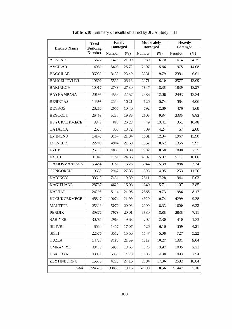
Table 5.10 Summary of results obtained by JICA Study [11]

Partly Damaged

Moderately Damaged

Heavily Damaged District Name

Total Building Number Number (%) Number (%) Number (%)

ADALAR 6522 1428 21.90 1089 16.70 1614 24.75

AVCILAR 14030 3609 25.72 2197 15.66 1975 14.08

BAGCILAR 36059 8438 23.40 3531 9.79 2384 6.61

BAHCELIEVLER 19690 5539 28.13 3171 16.10 2577 13.09

BAKIRKOY 10067 2748 27.30 1847 18.35 1839 18.27

BAYRAMPASA 20195 4559 22.57 2436 12.06 2493 12.34

BESIKTAS 14399 2334 16.21 826 5.74 584 4.06

BEYKOZ 28280 2957 10.46 792 2.80 476 1.68

BEYOGLU 26468 5257 19.86 2605 9.84 2335 8.82

BUYUKCEKMECE 3348 880 26.28 449 13.41 351 10.48

CATALCA 2573 353 13.72 109 4.24 67 2.60

EMINONU 14149 3104 21.94 1831 12.94 1967 13.90

ESENLER 22700 4904 21.60 1957 8.62 1355 5.97

EYUP 25718 4857 18.89 2232 8.68 1890 7.35

FATIH 31947 7781 24.36 4797 15.02 5111 16.00

GAZIOSMANPASA 56484 9181 16.25 3044 5.39 1888 3.34

GUNGOREN 10655 2967 27.85 1593 14.95 1253 11.76

KADIKOY 38615 7451 19.30 2811 7.28 1944 5.03

KAGITHANE 28737 4620 16.08 1640 5.71 1107 3.85

KARTAL 24295 5114 21.05 2365 9.73 1986 8.17

KUCUKCEKMECE 45817 10074 21.99 4920 10.74 4299 9.38

MALTEPE 25313 5070 20.03 2109 8.33 1600 6.32

PENDIK 39877 7978 20.01 3530 8.85 2835 7.11

SARIYER 30781 2965 9.63 707 2.30 410 1.33

SILIVRI 8534 1457 17.07 526 6.16 359 4.21

SISLI 22576 3512 15.56 1147 5.08 727 3.22

TUZLA 14727 3180 21.59 1513 10.27 1331 9.04

UMRANIYE 43473 5932 13.65 1725 3.97 1005 2.31

USKUDAR 43021 6357 14.78 1885 4.38 1093 2.54

ZEYTINBURNU 15573 4229 27.16 2704 17.36 2592 16.64

Total 724623 138835 19.16 62008 8.56 51447 7.10

100

CHAPTER 6

CONCLUSIONS AND RECOMMENDATIONS

6.1 SUMMARY

In this study, it is aimed to develop seismic damage estimation software, which is

capable of handling buildings individually. The software developed, named as “Seismic

Risk Analysis Software” (SRAS), uses the deterministic approach to predict the probable

damage distribution for a specified region caused by a deterministic earthquake. SRAS is

able to perform analysis using four attenuation relationships and three displacement

demand computation methods. The software has been verified by using it for the

estimation of damage distribution in Adapazarı due to August 17, 1999 Izmit Earthquake.

By means of spot checks of intermediate steps, the modules of SRAS have been

debugged. Then, considering unprecedented increase in the occurrence probability of a

large magnitude earthquake in the proximity of Istanbul within 30 years, SRAS has been

utilized for the estimation of probable damage distribution in Istanbul due to a scenario

earthquake (model A of JICA Study [11]) of moment magnitude 7.5.

6.2 CONCLUSIONS

Considering the analysis performed and keeping in mind that SRAS is a computer

program and it is the user responsibility to verify the reliability of the results produced by

SRAS, the following conclusions can be derived:

• Reliability of regional seismic damage estimation strongly depends on the quality

and accuracy of the data at hand. Dependable building inventory database is a

must to obtain realistic damage distribution for the region under consideration.

101

Site classification maps affect the results considerably and need to be developed

with special care. Capacity curve data are also crucial in performing the analysis

and capacity curves specific to each building should be used when available.

• SRAS has proved to be a reliable tool for performing lengthy calculations of

conventional regional assessment procedures. Provided that the input data are

dependable, SRAS produces same results (even more accurate in the case of

iterative methods) that should be obtained if hand calculation were preferred.

• SRAS has been developed to facilitate the usage of four attenuation relationships

(Abrahamson and Silva [20], Boore et al. [12], Gülkan and Kalkan [21] and

Sadigh et al. [16]) and three displacement demand computation procedures

(Capacity Spectrum Method (ATC-40 [8]), Displacement Coefficient Method

(FEMA-356 [19]) and Constant Ductility Method (Chopra and Goel [22]).

• Application of conventional regional damage estimation procedures to different

districts for several scenario earthquakes is faster and simpler by using SRAS.

Thus, researchers will have the opportunity of considering the effects of several

parameters such as attenuation relationship, analysis method, etc. to the regional

damage distribution pattern.

• SRAS has been developed as flexible as possible to make it handy not only for

districts in Turkey but also for different regions of the world. The user defines

capacity curve data peculiar to that region and a scenario earthquake fault. Then,

SRAS takes care of the numerous computations and time consuming database

operations.

• It should be noted that SRAS has been debugged by employing it just for two case

studies. The reliability and serviceability of the software can be further improved

if and only if SRAS is utilized by several users in different projects and feedback

is conveyed to the developer. This is the common way of debugging and

upgrading commercial software. Otherwise, SRAS will stay between the hard

covers of this thesis waiting for the day to be discovered.

6.3 RECOMMENDATIONS FOR FUTURE STUDY

• Probabilistic seismic hazard component may be added to facilitate the usage of

both seismic hazard assessment approaches under the same software structure.

This requires preparation of earthquake catalog data and source zones.

102

• Communication with commercial GIS applications such as ArcGIS and MapInfo

should be established for using powerful database operations provided by those

programs. Thus, preparation of database queries could be faster and easier.

• Computation of casualties and monetary losses due to the scenario earthquake

may also be integrated to the source code. As a consequence, an overall risk

assessment studio tool could be developed and used effectively.

• Capabilities of the software should be improved by appending more attenuation

relationships. Distance calculation algorithms may be revised for a better

performance. Default databases for capacity curves, damage curves, scenario

earthquake faults (including the past earthquakes) should be developed and

installed with SRAS.

• The software should be upgraded and new versions should be distributed in order

to track the most recent developments in seismic damage estimation area. Just as a

reminder, although many improvements had been done, SRAS will remain as a

computer program lacking of artificial intelligence. It is the user who leads SRAS.

103

REFERENCES

[1] ATC-13, 1985, Earthquake Damage Evaluation Data for California, Applied Technology Council, Redwood City, California.

[2] Whitman Robert V., Anagnos Thalia, Kircher Charles A., Lagorio Henry J.,

Lawson R. Scott, Schneider Philip, 1997, Development of a National Earthquake Loss Estimation Methodology, Earthquake Spectra, Vol. 13, No. 4, pp. 643-661, Oakland, CA: Earthquake Engineering Research Institute.

[3] Kircher Charles A., Reitherman Robert K., Whitman Robert V. and Arnold

Christopher, 1997, Estimation of Earthquake Losses to Buildings, Earthquake Spectra, Vol. 13, No. 4, pp. 703-720, Oakland, CA: Earthquake Engineering Research Institute.

[4] Federal Emergency Management Agency (FEMA), 1992, NEHRP Handbook for

the Seismic Evaluation of Existing Buildings, FEMA 178, Washington, D.C. [5] Frankel A., Mueller C., Barnhard T., Perkins D., Leyendecker E. V., Dickman N.,

Hanson S., and Hopper M., 1996, National Seismic-Hazard Maps: Documentation June 1996, USGS Open-File Report 96-532, Denver, CO, United States Geological Survey.

[6] Building Seismic Safety Council (BSSC), 1997, NEHRP Handbook for Seismic

Rehabilitation of Existing Buildings, Draft prepared for the Federal Emergency Management Agency, Washington, D.C.

[7] Federal Emergency Management Agency (FEMA), 1997, NEHRP Guidelines for

the Seismic Rehabilitation of Existing Buildings, FEMA 273, Washington, D.C. [8] Applied Technology Council (ATC), 1996, Seismic Evaluation and Retrofit of

Concrete Buildings Vol.1. Report No. SSC 96-01 (ATC-40).

104

[9] Kircher Charles A., Nassar Aladdin A., Kustu Onder and Holmes William T., 1997, Development of Building Damage Functions for Earthquake Loss Estimation, Earthquake Spectra, Vol. 13, No. 4, pp. 663-682, Oakland, California: Earthquake Engineering Research Institute.

[10] National Institute of Building Science (NIBS), 1997, Earthquake Loss Estimation

Methodology, HAZUS97: Technical Manual, Report prepared for the Federal Emergency Management Agency, Washington, D.C.

[11] Japan International Cooperation Agency (JICA) and Istanbul Metropolitan

Municipality (IMM), 2002, The Study on A Disaster Prevention / Mitigation Basic Plan in Istanbul including Seismic Microzonation in the Republic of Turkey, Final Report, December.

[12] Boore D.M., Joyner W.B., Fumal T.F., 1997, Equations For Estimating

Horizontal Response Spectra and Peak Acceleration From Western North American Earthquakes: A Summary of Recent Work, Seismological Research Letters, Vol. 68, No. 1, pp. 128-153, January/February.

[13] Boğaziçi University, Department of Earthquake Engineering, 2002, Earthquake

Risk Assessment for Istanbul Metropolitan Area, Final Report, KOERI (Kandilli Observatory and Earthquake Research Center), May.

[14] NEHRP, 1997, Recommended Provisions For Seismic Regulations For New

Buildings and Other Structures, FEMA-303, Prepared by the Building Seismic Safety Council for the Federal Emergency Management Agency, Washington, D.C.

[15] Federal Emergency Management Agency (FEMA), 1999, Earthquake Loss

Estimation Methodology, HAZUS99 Technical Manual, National Institute of Building Science, Washington, D. C.

[16] Sadigh K., Chang C.-Y., Egan J.A., Makdisi F., Youngs R.R., 1997, Attenuation

Relationships for Shallow Crustal Earthquakes Based on California Strong Motion Data, Seismological Research Letters Vol. 68(1), pp. 180-189, January/February

[17] Campbell, K. W., 1997, Empirical Near-Source Attenuation Relationships for

Horizontal and Vertical Components of Peak Ground Acceleration, Peak Ground Velocity, and Pseudo Absolute Acceleration Response Spectra, Seismological Research Letters Vol. 68(1), pp. 154-180, January/February

105

[18] Spudich, P., Joyner W.B., Lindh A.G., Boore D.M., Magraris B.M. and Fletcher J.B., 1999, SEA99: A Revised Ground Motion Prediction Relation for Use in Extensional Tectonic Regimes, Bull. Seism. Soc. Am., Vol. 89, No. 5.

[19] Federal Emergency Management Agency (FEMA), 2000, Prestandard and Commentary for the Seismic Rehabilitation of Buildings, Report FEMA 356, Washington, D.C

[20] Abrahamson N. A. and Silva W. J., 1997, Empirical Response Spectral

Attenuation Relations for Shallow Crustal Earthquakes, Seismological Research Letters, Vol. 68, No. 1, pp. 94-127, January/February.

[21] Gülkan P. and Kalkan E., 2002, Attenuation Modeling of Recent Earthquakes in

Turkey, Journal of Seismology, Vol. 6, pp. 397-409. [22] Chopra A. K. and Goel Rakesh K., 1999, Capacity-Demand-Diagram Methods

for Estimating Seismic Deformation of Inelastic Structures: SDF Systems, Report No. PEER-1999/02, Pacific Earthquake Engineering Research Center, College of Engineering, University of California, Berkeley.

[23] Newmark N. M. and Hall W. J., 1982, Earthquake Spectra and Design, Berkeley,

California, Earthquake Engineering Research Institute. [24] Krawinkler H. and Nassar A. A., 1992, Seismic design based on ductility and

cumulative damage demands and capacities. Nonlinear Seismic Analysis and Design of Reinforced Concrete Buildings, eds. P. Fajfar and H. Krawinkler. New York: Elsevier Applied Science.

[25] Vidic T., Fajfar P. and Fischenger N. M., 1994, Consistent inelastic design

spectra: strength and displacement, Earthquake Engineering and Structural Dynamics 23(5), pp.507-521

[26] Chopra A. K., 1995, Dynamics of Structures: Theory and Applications to

Earthquake Engineering, Chapters 3, 6, 7 and 19. Englewood Cliffs, N. J.: Prentice Hall.

[27] NEHRP, 2000, NEHRP Recommended Provisions For Seismic Regulations for

New Buildings And Other Structures, FEMA 368, Federal Emergency Management Agency (FEMA), Washington, D.C

106

[28] Turkish Ministry of Public Works and Settlement, 1997, Requirements for the Structures to be built in disaster areas, Ankara, Turkey.

[29] Yakut A., Ozturk, N. Y. and Bayili S., 2003, Analytical Assessment of Seismic

Capacity of RC Frame Buildings, Proceedings of the International Conference on Earthquake Engineering to Mark 40 Years from Catastrophic 1963 Skopje Earthquake and Successful City Reconstruction, Macedonia, Skopje, 26-29 August.

[30] Yakut A., Gülkan P., Bakır B. S. and Yılmaz M. T., Reexamination of Damage

Distribution in Adapazarı: Structural Considerations, (In Review), Engineering Structures.

[31] Parsons T., Toda S., Stein R.S., Barka A.A., and Dieterich J.H., 2000, Influence of

the 17 August 1999 Izmit Earthquake on Seismic Hazards in Istanbul, Manuscript accepted by JGR 2001.

107

APPENDIX A

SRAS MANUAL

INTRODUCTION

SRAS has been developed by Sezgin KUCUKCOBAN under supervision of Asst.

Prof. Dr. Ahmet YAKUT as a part of thesis study performed in Civil Engineering

Department of Middle East Technical University. The software is free of charge and can

be distributed freely for educational purposes. It is the responsibility of user to verify the

results generated by the software. This manual briefly describes the software interface,

details of creating and analyzing a project, output operations, general options and

limitations of the software. The information provided here is tried to be kept as concise as

possible in order to facilitate rapid screening of the manual. Just as a reminder, SRAS is

nothing but an ordinary computer program. It performs tiresome calculations for the user

and presents the results. It is the user who will criticize the reliability of these results.

Check for the updates from Internet or contact to ksezgin@metu.edu.tr.

INSTALLATION

To install SRAS:

1. Insert the CD into the CD-ROM drive. To start the installation process, from the

Start menu, choose Run. Enter the CD-ROM drive letter, and “SRAS\setup.exe”.

For example, enter “D:\SRAS\setup.exe”.

2. When “Welcome” page is displayed, choose OK.

3. Select an existing directory by clicking to “Change Directory” command button or

accept default directory.

108

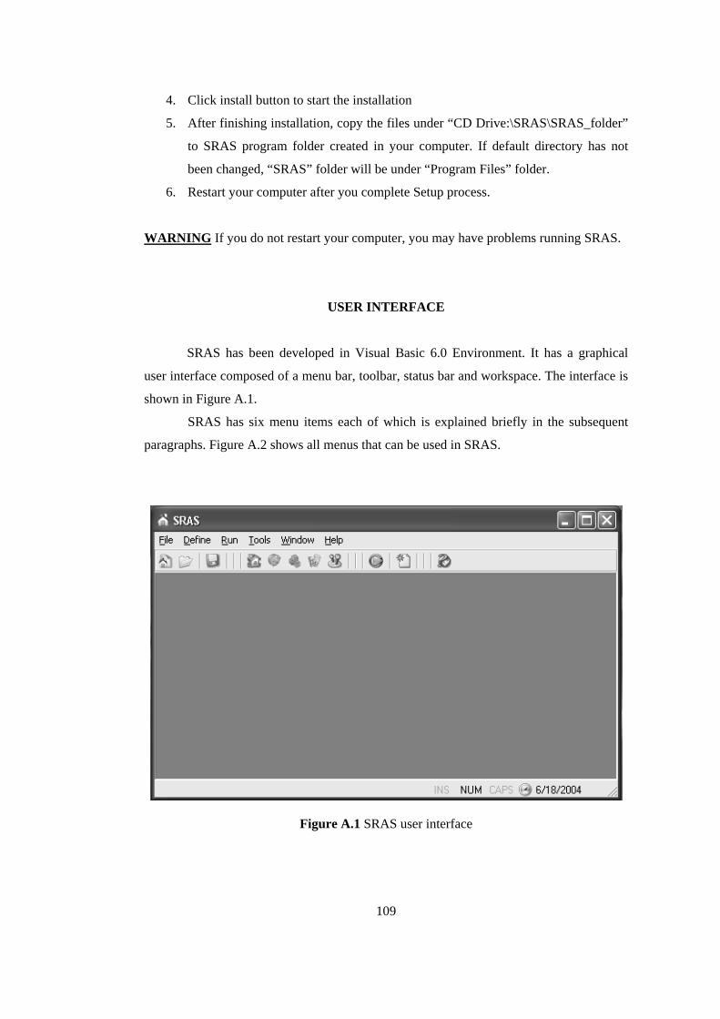
4. Click install button to start the installation

5. After finishing installation, copy the files under “CD Drive:\SRAS\SRAS_folder”

to SRAS program folder created in your computer. If default directory has not

been changed, “SRAS” folder will be under “Program Files” folder.

6. Restart your computer after you complete Setup process.

WARNING If you do not restart your computer, you may have problems running SRAS.

USER INTERFACE

SRAS has been developed in Visual Basic 6.0 Environment. It has a graphical

user interface composed of a menu bar, toolbar, status bar and workspace. The interface is

shown in Figure A.1.

SRAS has six menu items each of which is explained briefly in the subsequent

paragraphs. Figure A.2 shows all menus that can be used in SRAS.

Figure A.1 SRAS user interface

109

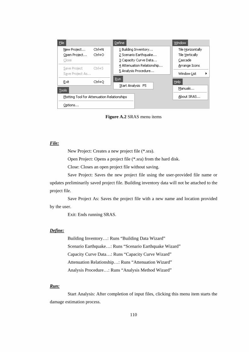
Figure A.2 SRAS menu items

File:

New Project: Creates a new project file (*.sra).

Open Project: Opens a project file (*.sra) from the hard disk.

Close: Closes an open project file without saving.

Save Project: Saves the new project file using the user-provided file name or

updates preliminarily saved project file. Building inventory data will not be attached to the

project file.

Save Project As: Saves the project file with a new name and location provided

by the user.

Exit: Ends running SRAS.

Define:

Building Inventory…: Runs “Building Data Wizard”

Scenario Earthquake…: Runs “Scenario Earthquake Wizard”

Capacity Curve Data…: Runs “Capacity Curve Wizard”

Attenuation Relationship…: Runs “Attenuation Wizard”

Analysis Procedure…: Runs “Analysis Method Wizard”

Run:

Start Analysis: After completion of input files, clicking this menu item starts the

damage estimation process.

110

Tools:

Plotting Tool for Attenuation Relationships: Runs a tool which takes moment

magnitude, distance (km) and average shear wave velocity (m/s) in order to compute

spectral acceleration values for the selected attenuation relationships.

Window:

Tile Horizontally: Arranges child windows horizontally.

Tile Vertically: Arranges child windows vertically.

Cascade: Arranges child forms in a stepwise manner.

Arrange Icons: Arranges minimized window icons.

Window List: Shows the list of open windows.

Help:

Manuals…: Runs windows explorer and opens manuals folder under software

root directory.

About SRAS…: Provides information about the software.

CREATING A NEW PROJECT

Using one of the following methods, you can create a new project.

1. Click “New Project…” menu item. 2. Click icon on the toolbar 3. Use “Ctrl + N” key combination

The screen, shown in Figure A.3, will appear and it will be labeled as “New

Project”.

111

Figure A.3 New project file

The project window is separated into three frames as INPUT, ANALYSIS and

RESULTS. INPUT frame collects required data for SRAS. ANALYSIS frame smoothes the

process of damage criteria selection and performs the analysis. RESULT frame presents,

exports and reports the computed results. Each part is discussed in the following sections.

INPUT frame: It contains five command buttons that are used for adding data

files to the current project. When the first button is clicked, the following screen will

appear.

112

Figure A.4 Add building inventory file window

The file list, located on the right, shows the content of “building_files” folder

under the root directory of SRAS. Building inventory files should have extensions of

(*.xls) and (*.mdb).

Add New File…: You may create a new building inventory file by using the

associated wizard. Clicking on this command button will activate the wizard. Detailed

information is provided in part describing “Wizards”.

Import File…: You may import a building inventory file, created in Excel or

Access, from a specified location. SRAS will create a copy of the selected file under

“building_files” folder. If you want to import several files simultaneously, open

“building_files” folder using windows explorer and paste here the copies of files to be

imported. Preparation of a new building inventory file is explained as a separate part.

Delete File: You can delete selected file from the disk. Please, be careful while

using this command, because undo is not available and the file will not be moved to

recycle bin.

113

Refresh List: After some file operations, the list should be refreshed to view the

changes in “building_files” folder.

OK: After selecting one of the files from the list, click this command button to

close the window and use the selected file in the analysis.

Cancel: Terminates the file adding porcess.

All buttons in the INPUT frame activates the same window by just changing

caption names and file filtering properties. Process, explained for the first button, is also

valid for the others. Interface differences are provided in the table below.

Table A.1 Interface differences between “Add … File” windows

Add … File Default File Folder File List Filter Associated Wizard

Building inventory Root\building_files *.xls or *.mdb Building Data Wizard

Scenario earthquake Root\scenario_files *.sef Scenario Earthquake Wizard

Attenuation relationship Root\atten_files *.att Attenuation Wizard

Analysis procedure Root\method_files *.apf Analysis Method Wizard

Capacity curve data Root\capa_files *.ccf Capacity Curve Wizard

After adding each file, a new command button will appear on the right. This

button is used for screening the data in the added file. It is also a verification showing that

SRAS has read the added file correctly and will run properly. Before passing to the

analysis stage, all data files must be added to the current project.

ANALYSIS

Prior to the analysis phase, all input data must be complete. Under ANALYSIS

frame, there are two damage estimation procedures available.

114

If “Based on Sd limits” is selected, the following window will appear.

Figure A.5 “Define Sd Limits” window

For each building type,

1. Enter a building type name. Building type names must be same (case

sensitive) with the ones defined in capacity curve file. Otherwise, damage

level assignment process can not be performed.

2. Enter number of damage levels (divisions). It can be any number between 3

and 9. For example, if damage levels of “Light”, “Moderate_1”,

“Moderate_2” and “Heavy” will be used, then 4 must be entered as number of

divisions. SRAS automatically creates a damage level named as “Collapse/No

Intersection” for those buildings fall beyond Sdmax.

3. Set damage limits by shifting those colorful bars to the left or right and

checking the formula provided. You may hold left mouse button pressed on

the bar and move the mouse left or right. Another way is to use arrow keys in

the keyboard after clicking on the bar. Do not change the given order of bars.

Use provided number-color twins not to mix up the sequence.

115

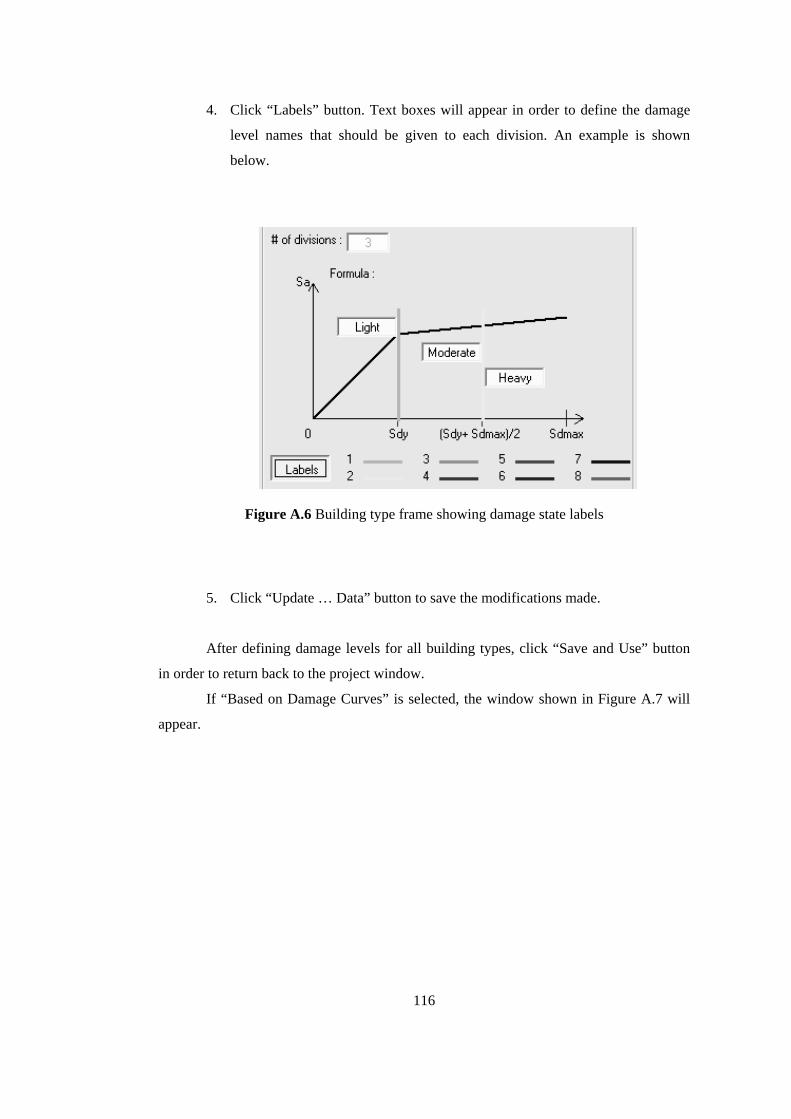
4. Click “Labels” button. Text boxes will appear in order to define the damage

level names that should be given to each division. An example is shown

below.

Figure A.6 Building type frame showing damage state labels

5. Click “Update … Data” button to save the modifications made.

After defining damage levels for all building types, click “Save and Use” button

in order to return back to the project window.

If “Based on Damage Curves” is selected, the window shown in Figure A.7 will

appear.

116

Figure A.7 “Define Damage Curves” window

For each building type,

1. Enter a building type name. Building type names must be same (case

sensitive) with the ones defined in capacity curve file. Otherwise, damage

level assignment process can not be performed.

2. Enter total number of damage curves. It can be any number between 1 and 9.

For example, if damage curves are available for story intervals of “1-4”, “4-

7”, “8-11” and “11-15”, then 4 must be entered as total number of curves.

Click OK.

3. SRAS automatically creates damage curve list depending on the provided

number. Select one of these curves. Enter for which interval the curve is valid

and upload text file including damage curve data.

4. Press “Update … data” button to save changes. Repeat steps 3 and 4 for other

curves and do not forget to update after changes made for each curve.

After defining damage curves for all building types, click “Save and Use” button

in order to return back to the project window.

Now you are ready to start analysis. The screen should look like as Figure A.8

before starting the analysis.

117

Figure A.8 The appearance of project file before starting the analysis

After clicking “Start Analysis” button, a window will be opened to show the

progress. An example screenshot is shown below subsequent to completion of analysis.

Figure A.9 Run window subsequent to completion of analysis

118

OUTPUT GENERATION

After completion of analysis, the command buttons in the “RESULTS” frame will

be enabled.

Figure A.10 “Results” frame after analysis has been completed

There are three things to do with the results.

• You can view tabular results in a window

• You can save results in a tabular format

• You can generate a report file for the project

Screen Display

This is the best way of rapid screening of results. Input-read errors can be easily

observed if there are any. An example of this tabular data view window is shown in Figure

A.11. You can use button to go to the previous record, button to go to the first

record, button to move to the next record, button to go to the final record in the

database. You may change the column widths. Editing the results is not allowed.

Export Results

It is possible to export the results tabulated in “View Results” window. There are

two different database formats that can be used while exporting the results. These are

Microsoft Excel and Access database formats. The exported files include everything

shown in “View Results” window. These exported files may be used for mapping or some

other type of post processing events.

119

Figure A.11 Tabular view of results

Generate Report

This extension prepares a report for the study performed. It includes every detail

regarding to the project except building inventory data. Instead of building database, a

table summarizing statistical distribution of buildings with respect to building type and

number of stories was presented. Scenario earthquake fault model, attenuation

relationship, analysis method and capacity curve data used in the project are added to the

report. Finally, “SiteLabel” based summary of results are written for each type o building

separately. For example, if “SiteLabel” was entered as district name, then the results will

be summarized in district level. You may use “_” character while combining district name

and sub-district names in order to perform a more refined analysis. For instance,

“ISTANBUL_KADIKOY” can be used as “SiteLabel” to facilitate the generation of

summary in sub-district level.

120

The report includes some other parameters such as report title and user

information (this is explained in GENERAL OPTIONS). Summary of results is only

written to the report when SDL method is selected for damage estimation. If DC method is

preferred, report file will not give any information regarding to the results obtained. It will

be a collection of input parameters used for that project.

There are two formats that are supported by SRAS: “Text File” and “Microsoft

Word Document” having extensions of (*.txt) and (*.doc), respectively. Creation of word

document may sometimes lead errors, so it is better to prefer text file format. Word

document file generation takes longer time due to formatting such as insertion of tables

and pictures. On the other hand text files are created almost instantaneously for small

databases and require comparatively less time than word documents for large databases.

GENERAL OPTIONS

SRAS has a few general options that should be modified or kept as they were

before starting to use the application. Select “Tools” menu and click on “Options…” menu

item. Options window will be shown. There are two tabs: “User Details” and

“Modification Factors”. In order to make changes in the user profile, select “User Details”

tab and enter any valid data to the textboxes. A screenshot is provided in Figure A.12.

Then click “Apply” command button to make changes permanent.

Figure A.12 “User Details” tab in “Options” windows

121

The process is also valid for modification factor changes. Click on “Modification

Factors” tab. You may change default coefficients that are used to modify calculated

spectral displacement values considering apparent condition and construction date. Do not

forget to click “Apply” if you have made any edits.

Figure A.13 “Modification Factors” tab in “Options” menu

TOOLS

A plotting tool for attenuation relationships is attached to the software for rapid

visualization of spectral acceleration curve. Select “Tools” menu and click “Plotting Tool

for Attenuation Relationships” menu item. The screen shown in Figure A.14 will appear.

Enter values for distance, shear wave velocity and moment magnitude. Select

attenuation relationship and fault type. Then click “Plot” command button. You may plot

all four graphs on the same plot. If you want to find out the values click on a point on the

graphs and read the values from the right-bottom part having light yellow background. In

order to save the coordinates of spectral acceleration curves, click “Save” command

button and export results as a text file.

122

Figure A.14 “Plotting Tool for Attenuation Relationships” window

SRAS LIMITATIONS

SRAS is capable of handling large databases but the running time mostly depends

on the hardware configuration details of the computer. SRAS has been developed only for

four attenuation relationships and three demand displacement computation methods.

These are:

Attenuation Relationships:

1. Abrahamson and Silva [20] 2. Boore et al. [12] 3. Gülkan and Kalkan [21] 4. Sadigh et al. [16]

Analysis Methods:

1. Capacity spectrum method of ATC-40 [8] 2. Displacement coefficient method of FEMA-356 [19] 3. Constant ductility method proposed by Chopra and Goel [22]

123

Limitations that are inherit in attenuation relationships and analysis methods are

also valid for SRAS. Be careful to select the proper attenuation relationship and analysis

method. Regarding to the capacity curve data, SRAS supports up to 15 building types.

This limit can be easily increased in the next versions.

SRAS WIZARDS

1. Define New Building Inventory Data File

a. On the Define menu, click Building Inventory.

b. Select program type for which this data will be used and file type in which

format this data will be saved, then click Next.

c. Enter required information for the first building.

d. Repeat step c until data for all buildings that are going to be analyzed are

written to the table. After finishing, click Next.

e. Enter a name for generated building inventory file considering file-naming

limitations of Windows.

2. Define New Scenario Earthquake File

a. On the Define menu, click Scenario Earthquake.

b. Select the fault model to be used in the calculations. Click Next.

c. If you have selected “linear fault”, enter spatial coordinates of each node.

Nodes must be in numerical order as 1, 2, 3….

d. If you have selected “meshed fault”, besides spatial coordinates of nodes, a

mesh size should be entered for each segment. Click a mesh size cell. An input box will

appear. Enter mesh size for that segment and repeat this procedure for all other segments.

Then, click Next.

e. The tabulated information about all segments is displayed. Enter a moment

magnitude for the scenario earthquake. Click Next.

f. Enter a name for generated fault model considering file-naming limitations of

Windows.

3. Define New Capacity Curve Data File

a. On the Define menu, click Capacity Curve Data.

b. Enter building type names for database creation. Click Next.

124

c. Select building type. Add capacity curve data for buildings having number of

stories “From” … “To” …. Capacity curve data for interior number of stories will be

generated automatically from the boundary values.

d. After finishing addition, do not forget to assign! Repeat step 3 and 4, until

capacity curve data for all defined building types are defined. Click Next.

e. Enter a name for generated capacity curve data file considering file-naming

limitations of Windows.

4. Define New Attenuation Relationship File

a. On the Define menu, click Attenuation Relationship.

b. Select an attenuation relationship. Read the provided information carefully in

order to select the most appropriate relationship for analysis. Click Next.

c. Select faulting style. Click Next.

d. Select site classification scheme. There are two schemes available in this

version. Site class definitions are provided below. You should use default “ID” values

while entering site classes in the building data input file. Be sure that you have selected

the correct scheme which is used during the preparation of input file. Click Next.

e. Enter a name for generated attenuation model considering file-naming

limitations of Windows.

5. Define New Analysis Method File

a. On the Define menu, click Analysis Procedure.

b. Select an analysis method. There are three methods available in this version.

Click Next.

c. Enter required information for that model. Click Next.

d. Enter a name for generated analysis model considering file-naming limitations

of Windows.

PREPARING A BUILDING INVENTORY FILE

SRAS is capable of handling database files that have extensions *.xls and *.mdb.

Although it supports Microsoft Excel files created in XP and previous versions, it gives

support only for Access database files created in or exported to 97 format. While

125

preparing building inventory files, the procedure differs slightly. Please, read and apply

the procedures very carefully to facilitate error-free analysis by SRAS.

Using Microsoft Excel:

1. Open a new Excel Worksheet.

2. Rename one of the sheets as “BD” (referring to building database) and delete the

other sheets. (It is crucial to rename the sheet as “BD”. Other names will lead

errors.)

3. Starting from cell “A1” write the field names for the following fields. Any name

can be used for the fields provided that it is free of special characters such as “+ , .

/ \ [ ] ? ! & % ( ) ’ = < > | ~ : ; £ # $ { }”. Underscore “_” should be used instead

of spacing character. The order of fields must not be changed. If a field is empty,

write field name and leave that column blank.

Table A.2 List of field types for building input file (Excel)

Order Field Name Field Type

1 SiteID Long Integer

2 SiteLabel String * 100

3 BuildingLabel String * 100

4 Latitude Double

5 Longitude Double

6 SiteClass Single

7 NumberOfStories Integer

8 BuildingType String * 15

9 NumberOfBuildings Single

10 ConstructionYear Integer

11 Condition Integer (!!!)

12 Information String * 100

!!! : (1=Very Poor, 2=Poor, 3=Moderate or 4=Good)

4. Write data for each building or building group and save your building inventory

file.

126

NOTE: If there is an available building inventory database, modify the field

characteristics and sequence in order to satisfy the requirements specified above for the

use in SRAS.

Using Microsoft Access:

1. Open a new access database file.

2. Insert a new table named as “BD”. (It is crucial to rename the database table as

“BD”. Other names will lead errors.)

3. Starting from first field, create the following fields using “Table Designer tool of

Access. Provide specific information about filed types. The order of fields must

not be changed. If a field is empty, write field name and leave that column blank.

(Please, be careful that Access takes “0” as the default value of generated number

fields. Clear “0” from the default value textbox before proceeding to the next

field.)

Table A.3 List of field types for building input file (Access)

Order Field Name Field Type

1 SiteID Long Integer

2 SiteLabel String * 100

3 BuildingLabel String * 100

4 Latitude Double

5 Longitude Double

6 SiteClass Single

7 NumberOfStories Integer

8 BuildingType String * 15

9 NumberOfBuildings Single

10 ConstructionYear Integer

11 Condition Integer (!!!)

12 Information String * 100

!!!: (1=Very Poor, 2=Poor, 3=Moderate or 4=Good)

4. Write data for each building or building group and save your building inventory

file.

127

5. Then using “Convert Database” tool of Microsoft Access, convert the generated

database table to Access 97 format. Microsoft Access will give you a message

saying that you will lose some properties of the database. Click OK to proceed.

NOTE: If there is an available building inventory database, modify the field

characteristics and sequence in order to satisfy the requirements specified above for the

use in SRAS.

128

APPENDIX B

CASE STUDY: ADAPAZARI

Table B.1 GDDA database damage statistics [30]

Collapsed and Heavily Damaged

Moderately and Lightly Damaged ID District

Number % Number %

Total

1 Maltepe 0 0 42 100 42 2 Hızırtepe 0 0 12 100 12 3 Şirinevler 9 35 17 65 26 4 Güllük 4 36 7 64 11 5 Mithatpaşa 23 14 139 86 162 6 Yenidoğan 101 57 75 43 176 7 Papuçcular 53 38 87 62 140 8 Akıncılar 13 33 27 68 40 9 Yenicami 26 48 28 52 54

10 Çukurahmediye 3 19 13 81 16 11 Semerciler 55 29 135 71 190 12 Tığcılar 19 10 163 90 182 13 Yenigün 78 19 336 81 414 14 Tepekum 5 8 60 92 65 15 Şeker 111 40 168 60 279 16 Cumhuriyet 31 22 111 78 142 17 Orta Mahalle 17 13 117 87 134 18 Yahyalar 14 16 72 84 86 19 Yağcılar 9 6 142 94 151 20 Kurtuluş 5 13 33 87 38 21 İstiklal 8 13 55 87 63 22 Karaosman 29 38 47 62 76 23 Ozanlar 12 15 69 85 81 24 Sakarya 4 11 33 89 37 25 Tekeler 7 7 87 93 94 26 Tuzla 2 13 13 87 15

Total 638 2088 2726

129

Table B.2 Predicted damage for the GDDA dataset based on soft soil type and Gülkan and

Kalkan [21] attenuation relationship

Damage Distribution(%) ATC-40 FEMA-273 Chopra & Goel ID District

L M H L M H L M H 1 Maltepe 0 0 100 0 0 100 0 100 0

2 Hızırtepe 0 0 100 0 0 100 0 100 0

3 Şirinevler 0 0 100 0 0 100 0 100 0

4 Güllük 0 0 100 0 0 100 0 100 0

5 Mithatpaşa 0 100 0 0 0 100 0 100 0

6 Yenidoğan 0 100 0 0 0 100 0 100 0

7 Papuçcular 0 100 0 0 0 100 0 100 0

8 Akıncılar 0 100 0 0 0 100 0 100 0

9 Yenicami 0 100 0 0 0 100 0 100 0

10 Çukurahmediye 0 100 0 0 0 100 0 100 0

11 Semerciler 0 100 0 0 30 70 0 100 0

12 Tığcılar 0 100 0 0 58 42 0 100 0

13 Yenigün 0 100 0 0 0 100 0 100 0

14 Tepekum 0 100 0 0 51 49 0 100 0

15 Şeker 0 100 0 0 78 22 0 100 0

16 Cumhuriyet 0 100 0 0 43 57 0 100 0

17 Orta Mahalle 0 100 0 0 36 64 0 100 0

18 Yahyalar 0 100 0 0 42 58 0 100 0

19 Yağcılar 0 100 0 0 100 0 0 100 0

20 Kurtuluş 0 100 0 0 11 89 0 100 0

21 İstiklal 0 100 0 0 95 5 0 100 0

22 Karaosman 0 100 0 0 92 8 0 100 0

23 Ozanlar 0 100 0 0 100 0 0 100 0

24 Sakarya 0 100 0 0 100 0 0 100 0

25 Tekeler 0 100 0 0 100 0 0 100 0

26 Tuzla 0 100 0 0 100 0 0 100 0

130

Figure B.1 PGA distribution obtained for different attenuation relationships

131

Figure B.2 Distribution of Sa values at T = 0.3 s and 1.0 s for two attenuation relations

132

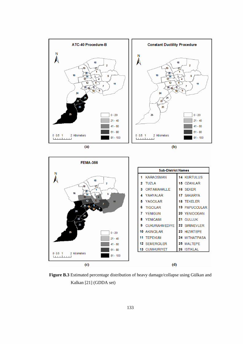
Figure B.3 Estimated percentage distribution of heavy damage/collapse using Gülkan and

Kalkan [21] (GDDA set)

133

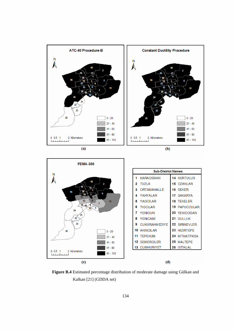
Figure B.4 Estimated percentage distribution of moderate damage using Gülkan and

Kalkan [21] (GDDA set)

134

Figure B.5 Estimated damage for SU database based on soft soil using Boore et al. [12]

135

APPENDIX C

CASE STUDY: ISTANBUL

0

0.1

0.2

0.3

0.4

0.5

0.6

0.7

0.8

0.9

0 2 4 6 8 10 12 14 16 18

Sd (cm)

Sa (g

)

JICA 1F - 3FJICA 4F - 7FJICA 8F -New 1F - 3FNew 4F - 7FNew 8F -

Figure C.1 A sample group of capacity curves for RC buildings

136

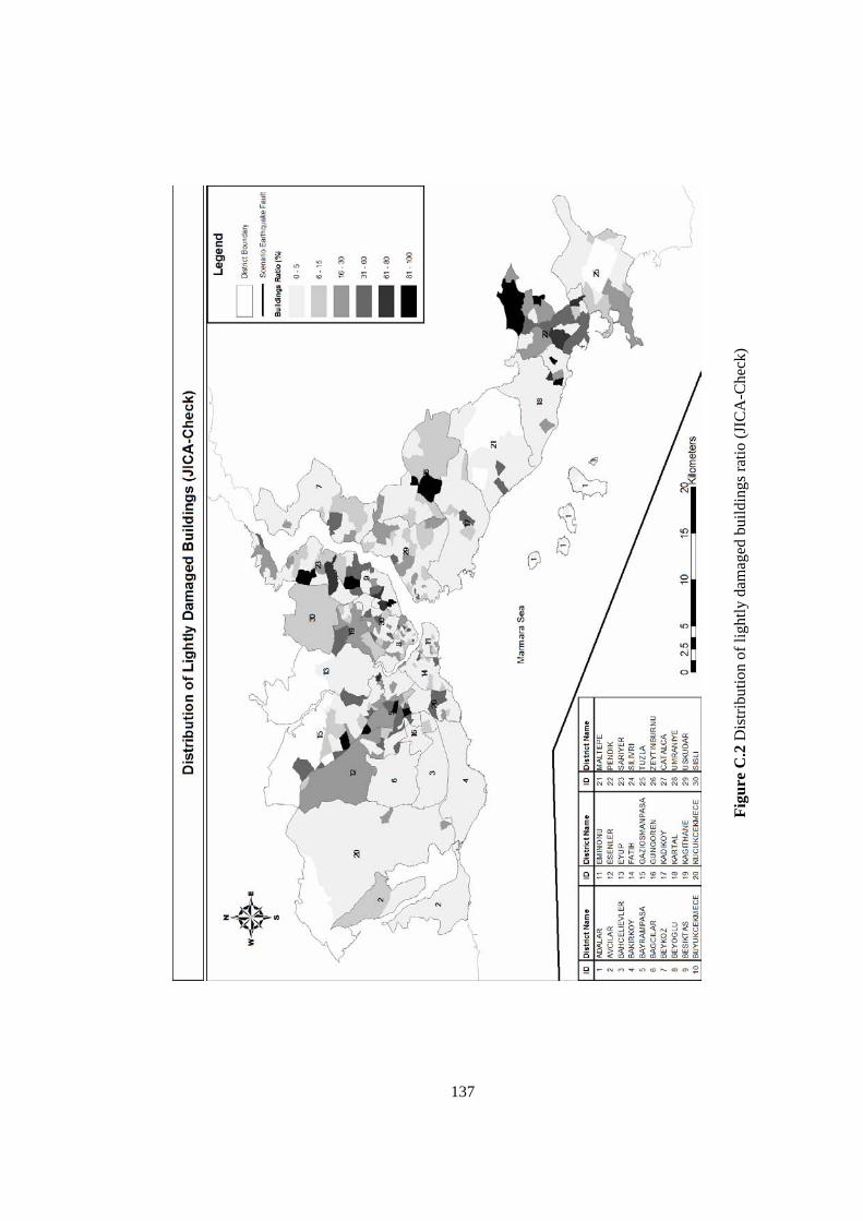
Figu

re C

.2 D

istri

butio

n of

ligh

tly d

amag

ed b

uild

ings

ratio

(JIC

A-C

heck

)

137

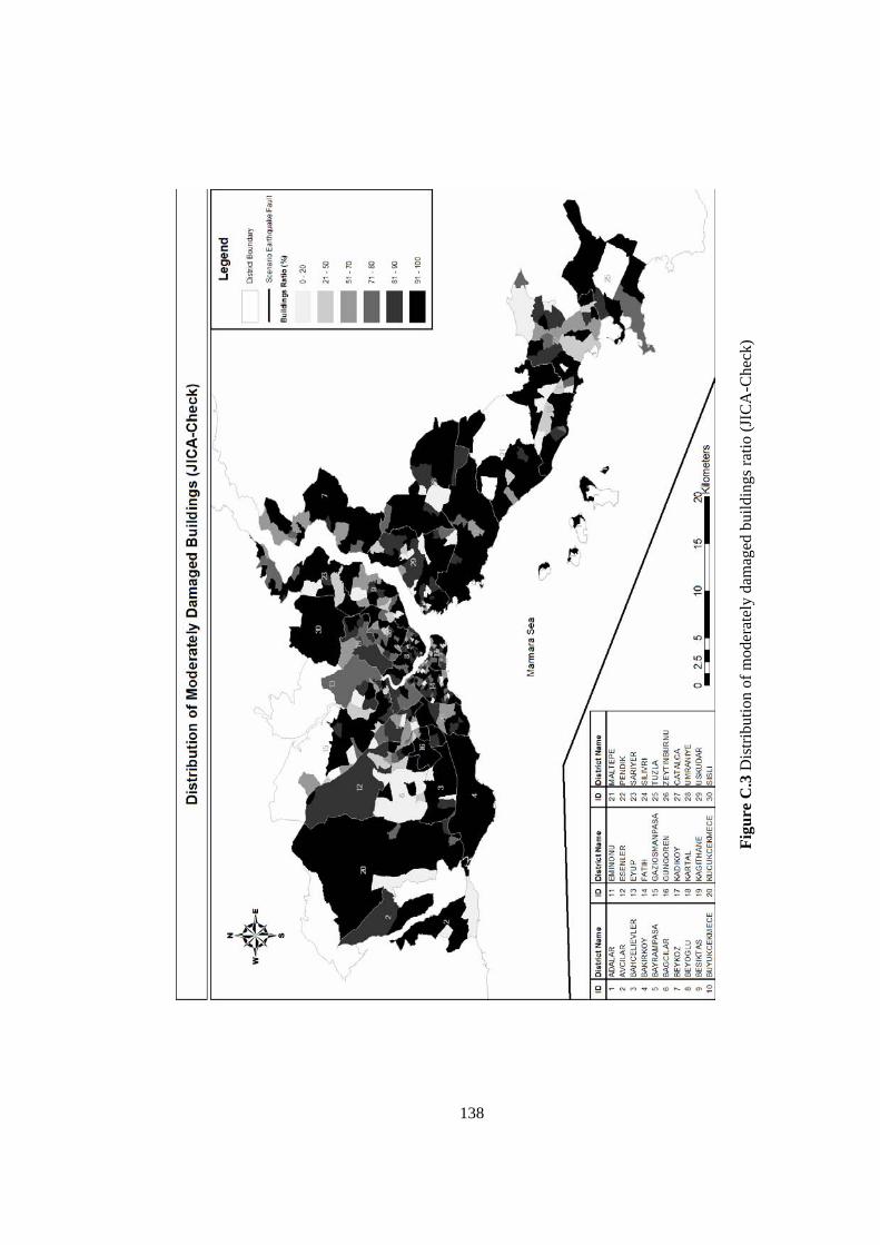
Figu

re C

.3 D

istri

butio

n of

mod

erat

ely

dam

aged

bui

ldin

gs ra

tio (J

ICA

-Che

ck)

138

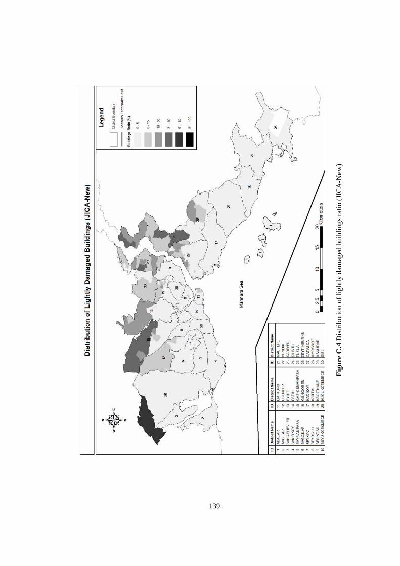
Figu

re C

.4 D

istri

butio

n of

ligh

tly d

amag

ed b

uild

ings

ratio

(JIC

A-N

ew)

139

Figu

re C

.5 D

istri

butio

n of

mod

erat

ely

dam

aged

bui

ldin

gs ra

tio (J

ICA

-New

)

140

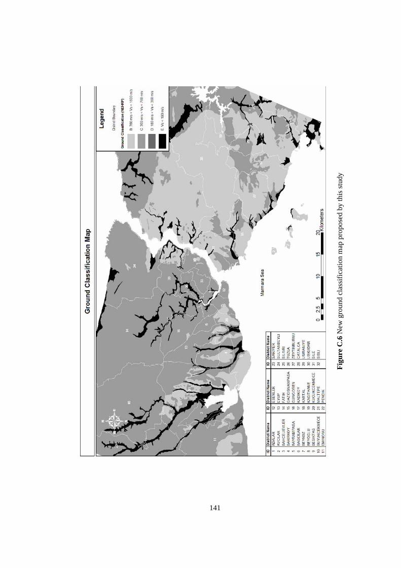
Figu

re C

.6 N

ew g

roun

d cl

assi

ficat

ion

map

pro

pose

d by

this

stud

y

141

Figu

re C

.7 D

istri

butio

n of

pea

k gr

ound

acc

eler

atio

n (I

MM

-New

)

142

Figu

re C

.8 D

istri

butio

n of

Sa v

alue

s at t

he p

erio

d of

0.3

sec

(IM

M-N

ew)

143

Figu

re C

.9 D

istri

butio

n of

Sa v

alue

s at t

he p

erio

d of

1.0

sec

(IM

M-N

ew)

144

Figu

re C

.10

Dis

tribu

tion

of li

ghtly

dam

aged

bui

ldin

gs ra

tio (I

MM

-New

)

145

Figu

re C

.11

Dis

tribu

tion

of m

oder

atel

y da

mag

ed b

uild

ings

ratio

(IM

M-N

ew)

146

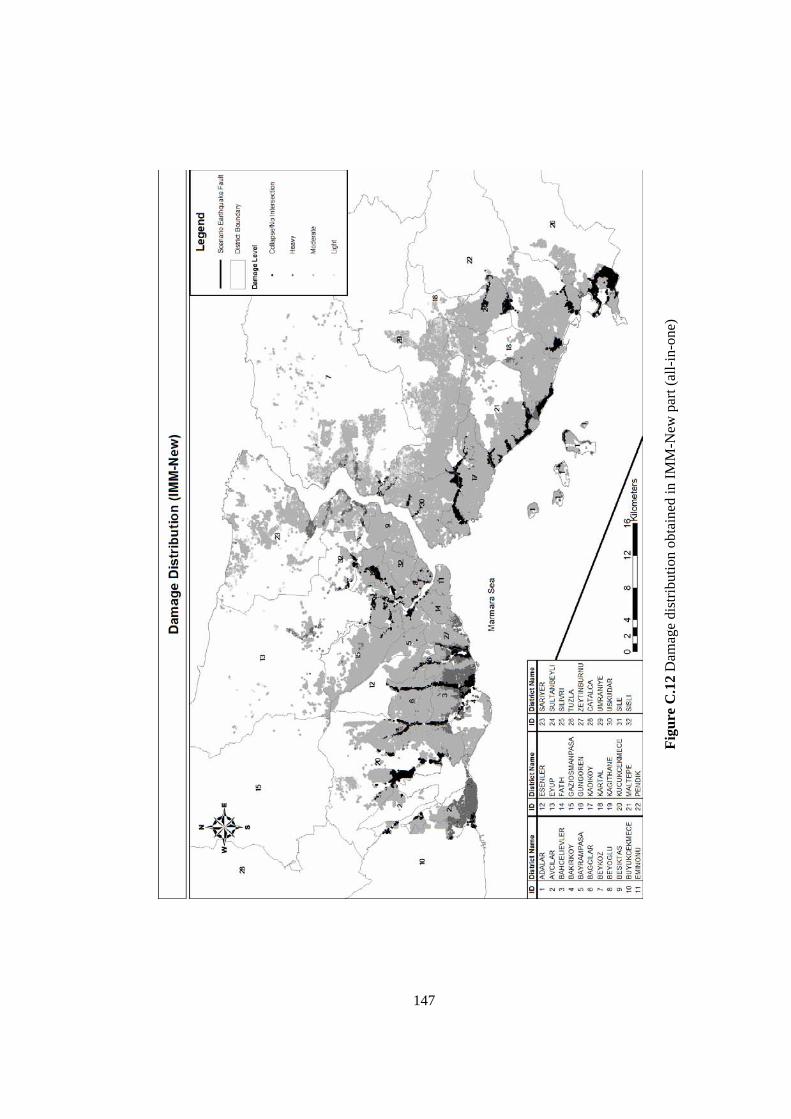
Figu

re C

.12

Dam

age

dist

ribut

ion

obta

ined

in IM

M-N

ew p

art (

all-i

n-on

e)

147