development of an edys ecological model of the … · 2017-06-20 · development of an edys...
TRANSCRIPT

DEVELOPMENT OF AN EDYS ECOLOGICAL MODEL OF THE UPPER LLANO RIVER WATERSHED AND EVALUATION OF POTENTIAL ENHANCEMENT OF
WATER YIELD FROM BRUSH CONTROL
FINAL REPORT
PREPARED FOR:
TEXAS STATE SOIL AND WATER CONSERVATION BOARD
Terry McLendon, Jon D. Booker, Cade L. Coldren, Cindy R. Pappas, and Kenneth A. Rainwater
TEXAS TECH UNIVERSITY
April 2017

Upper Llano River EDYS Model FINAL REPORT April 2017
1
TABLE OF CONTENTS EXECUTIVE SUMMARY --------------------------------------------------------------------------------------- 2 1.0 INTRODUCTION -------------------------------------------------------------------------------------------- 6 2.0 SPATIAL FOOTPRINT ------------------------------------------------------------------------------------- 7 3.0 TOPOGRAPHY ----------------------------------------------------------------------------------------------- 8 4.0 PRECIPITATION --------------------------------------------------------------------------------------------- 10 4.1 Temporal Variability ------------------------------------------------------------------------------------- 10 4.2 Spatial Variability ---------------------------------------------------------------------------------------- 14 4.3 Constructed Precipitation Data Sets ------------------------------------------------------------------- 18 4.4 Precipitation Regimes by Spatial Segment ----------------------------------------------------------- 25 5.0 SOILS ----------------------------------------------------------------------------------------------------------- 26 5.1 Soils Map -------------------------------------------------------------------------------------------------- 26 5.2 Profile Descriptions -------------------------------------------------------------------------------------- 28 6.0 VEGETATION ------------------------------------------------------------------------------------------------ 32 6.1 Selection of Plant Species ------------------------------------------------------------------------------- 32 6.2 Plant Parameter Variables ------------------------------------------------------------------------------- 34 6.3 Plant Communities --------------------------------------------------------------------------------------- 39 6.3.1 Terrestrial Vegetation ---------------------------------------------------------------------------- 39 6.3.2 Land-Use Types ----------------------------------------------------------------------------------- 44 6.3.3 Aquatic Types ------------------------------------------------------------------------------------- 45 7.0 ANIMALS ------------------------------------------------------------------------------------------------------ 47 7.1 Insects ------------------------------------------------------------------------------------------------------ 47 7.2 Rabbits ----------------------------------------------------------------------------------------------------- 47 7.3 White-tailed Deer ----------------------------------------------------------------------------------------- 48 7.4 Cattle ------------------------------------------------------------------------------------------------------- 48 7.5 Sheep and Goats ------------------------------------------------------------------------------------------ 50 7.6 Feral Hogs ------------------------------------------------------------------------------------------------- 50 8.0 CALIBRATION ----------------------------------------------------------------------------------------------- 50 8.1 Vegetation ------------------------------------------------------------------------------------------------- 51 8.1.1 General Procedure -------------------------------------------------------------------------------- 51 8.1.2 Examples ------------------------------------------------------------------------------------------- 52 8.2 Ecohydrology --------------------------------------------------------------------------------------------- 62 8.2.1 Evapotranspiration -------------------------------------------------------------------------------- 62 8.2.2 Surface Runoff ------------------------------------------------------------------------------------ 66 8.2.3 Groundwater Use --------------------------------------------------------------------------------- 68 9.0 SCENARIO RESULTS -------------------------------------------------------------------------------------- 69 9.1 Effects of Precipitation Regime ------------------------------------------------------------------------ 69 9.1.1 Vegetation ----------------------------------------------------------------------------------------- 69 9.1.2 Ecohydrology ------------------------------------------------------------------------------------- 74 9.2 Watershed-Wide Ecohydrology: Baseline Conditions ---------------------------------------------- 75 9.3 Watershed-Wide Ecohydrology: Brush Control Scenario ------------------------------------------ 80 9.4 Selection of Subwatersheds for Treatment ----------------------------------------------------------- 82 10.0 LITERATURE CITED ------------------------------------------------------------------------------------- 88 APPENDIX A: PRECIPITATION ------------------------------------------------------------------------------ 104 APPENDIX B: VEGETATION ---------------------------------------------------------------------------------- 113 APPENDIX C: PLANT PARAMETERS ---------------------------------------------------------------------- 126 APPENDIX D: ANIMALS --------------------------------------------------------------------------------------- 160

Upper Llano River EDYS Model FINAL REPORT April 2017
2
EXECUTIVE SUMMARY The Llano River is one of the major rivers flowing through the Edwards Plateau of Texas, supplying water to the region as well as being a major contributor to the Greater Colorado River Watershed, one of the largest river systems of Texas. The North Llano and South Llano Rivers form the headwaters of the Llano River, with the two rivers converging near Junction, Texas to form the Llano River. The Texas State and Soil and Water Conservation Board (TSSWCB) was a major contributor to the development of the Upper Llano Watershed Protection Plan. Part of the role of TSSWCB was to provide quantitative estimates of the impacts of various land management practices and natural climatic fluctuations on the surface water and groundwater supplies affecting the Upper Llano River system. These estimates were produced by use of the ecological simulation model EDYS. In addition, TSSWCB is interested in the development of county-wide simulation models to evaluate potential enhanced water yields from control of woody species. To meet both these needs, an EDYS model was developed for the Upper Llano River Watershed. This report presents a description of this model and results of simulations evaluating the potential for enhanced water yields from brush control. Description of the Model The spatial domain of the model is the combined watersheds of the North Llano and South Llano Rivers. It includes large portions of four counties (Edwards, Kimble, Real, and Sutton) and smaller portions of another three counties (Kerr, Menard, and Schleicher). The entire area included in the model footprint is about 2625 mi2 (1.7 million acres), located in the southwestern part of the Edwards Plateau. The basic spatial unit of the EDYS model is the cell, the size of which is flexible. The basic cell size in the Upper Llano model is 40 m x 40 m (0.40 acre). This resulted in an overall spatial footprint of 4.2 million cells. To improve run times and reduce memory requirements, six separate models were constructed for the Upper Llano watershed, three modeling the uplands and three modeling the rivers and floodplains. The six models were linked to form a single overall functional model, with the upland models using the 40 m x 40 m cell sizes and the river and floodplain models using a 10 m x 10 m cell grid to more precisely simulate dynamics in these wetland sites. Surface topography in the model is defined by an average elevation for each cell, with slope and aspect determined by differences in elevation among adjacent cells, using USGS 10-m DEM data. Each cell also has an average depth to groundwater value, from which a depth to groundwater grid was defined for the entire model footprint. The spatial domain was divided into seven precipitation zones, with separate precipitation files used for the cells in each zone. The model simulates rainfall on a daily basis. For each of the seven zones, a 120-year (1893-2012) daily precipitation record was created based on statistical relationships among recorded precipitation data from 20 stations in a 10-county region. A detailed soil profile description was assigned to each of the 4.2 million cells in the model. These profiles were developed from NRCS soil survey descriptions of the included counties and from additional data available in the literature. A total of 48 soil types are included in the Upper Llano model and each cell is assigned one of the 48 soils based on the location of the cell on the spatial landscape. Each of the 48 soil types is divided into 20 layers, with the thickness and physical and chemical characteristics of each layer varying among the types. Some of the soil variables remain constant throughout a simulation (e.g., soil texture) while values of other variables (e.g., soil moisture) change by layer on a daily basis depending on environmental factors such as amount of rainfall received and amount of water and nutrients extracted by plants.

Upper Llano River EDYS Model FINAL REPORT April 2017
3
The number of plant species included in a specific EDYS application is flexible. A total of 51 species are included in the Upper Llano model. Dynamics of each species are modeled by use of 346 parameter variables, with each variable having different values for each species. Changes in vegetation are modeled in EDYS on a plant species (or plant part) basis by simulating differential responses, defined by the different parameter values, to changes in environmental factors (e.g., rainfall, grazing, season). The spatial footprint of the model was divided into plant communities and land management units (e.g., cultivated, orchards, urban) by assigning each cell type to one of 63 plot types (upland vegetation, aquatic vegetation, and land-use types). The locations of the land-use types were based on 2012 NAIP aerial photographs and the locations of the vegetation types were based on NRCS soil survey maps, with some adjustment based on the NAIP aerial photographs. Each vegetation type was further divided based on amount of woody plant cover present, with these values visually estimated from the NAIP aerial photographs. Initial (i.e., start of each simulation) biomass values were entered for each plant species in each plot type based on species composition of each type. Biomass (above- and belowground) values change for each plant species and each plant part (e.g., fine roots, trunks, leaves) per species at each time step (daily) during an EDYS simulation. The animal component in EDYS models consists of the effects of herbivory by different types of animals, both domestic and wildlife, on the vegetation. Herbivory is modeled as a plant-part and plant-species specific process, where selection of plant parts and plant species varies by animal species. Densities of each animal species are entered, and the model calculates the quantity of plant material the animals would consume daily and then determines how much of each species is removed based on selectivity, accessibility, and competitiveness among the animals. Four animal species (or groups) were included in the Upper Llano models: cattle, white-tailed deer, cottontail rabbits, and insects. Cattle were used to represent livestock because of lack of specific ratios of cattle, sheep, and goats for each ranch in the spatial domain. An average white-tailed deer density of 1 deer per 10 acres was used in the model. Cattle stocking rates were calculated for each vegetation type and averaged 24-33 ac/AU (varied between 7-106 ac/AU) for native rangeland across the four counties. Calibration Calibration in EDYS consists of making adjustments to parameter values, if needed, to achieve target values for the output variables under consideration. Target values are taken from independent validation data, either experimental validation studies or existing field data, if these data are available. In the absence of independent validation data, values from the literature and values based on professional judgment are used. Independent validation data were not available for the use in the Upper Llano models. Therefore, data from published studies in the Edwards Plateau and adjacent regions and professional judgment were used to calibrate the vegetation and hydrologic dynamics of the models. Ten-year simulations for six plot types (plant communities) were used in the vegetation calibration process. Results of simulated vegetation change in response to fluctuations in rainfall, time (succession), and grazing were compared to published results from 16 studies and to our professional experience in the region. The simulation results compared favorably with the patterns and levels expected from these studies and regional experience. Overall, there was an increase in trees, primarily Ashe juniper and mesquite, over time. This is expected in a woodland-grassland ecotone in the absence of fire. Grasses increased under average and wet precipitation regimes but decreased on most sites under the dry regime. In proportion to initial values, cane bluestem was the midgrass species that had the greatest increase and purple threeawn and curly mesquite were the shortgrasses with the greatest increase in biomass.

Upper Llano River EDYS Model FINAL REPORT April 2017
4
Three ecohydrological components were assessed in the model calibration: 1) evapotranspiration (ET), 2) surface runoff, and 3) groundwater use by vegetation. The ecohydrological calibration data were taken from the same six plot types used in the vegetation calibration. Average annual ET on the six types varied between 15.4 and 27.9 inches. Overall, this was equal to 94.4% of annual precipitation under the average precipitation regime. This compares with reported values of 95% for an oak-grassland on the Sonora Experiment Station and 93% for mesquite-grasslands in the Rolling Plains. Simulated daily ET rates on the clay loam type (38% woody cover) averaged 1.7 mm (12-month basis) or 2.5 mm (growing season basis), compared to literature values of 1.7-2.6 mm for mesquite grasslands and 2.8 mm (growing season basis) for an Ashe juniper woodland in the eastern Edwards Plateau. Runoff from the relatively level types in the simulations averaged 0.3-0.5 inch per year, which is similar to reported values in the literature of 0.2-1.2 inches for similar sites. Runoff was higher from the steeper-slope sites, averaging 2.8 inches per year. Literature values for juniper sites in the Edwards Plateau are in the range of 1.1-1.9 inches per year. The two upland types in the calibration simulations did not utilize any groundwater. However, groundwater use by vegetation in the other four types averaged 1.4 inches per year, or about 6% of annual transpiration on these sites. Results Four 25-year simulation scenarios were conducted to evaluate the response of the Upper Llano subwatersheds to fluctuations in precipitation and to evaluate the potential for enhanced water supply from brush control. Scenario 1 was the baseline scenario where the average precipitation regime (the 25 continuous years that had overall average annual precipitation nearest to the long-term annual average precipitation) was used with no brush control. Scenario 2 was the same as Scenario 1 except the driest 25-year precipitation regime was used. Scenario 3 was also the same as Scenario 1 except the wettest 25-year precipitation regime was used. Scenario 4 used the average precipitation regime, but brush control was added. The brush control option consisted of removing 100% of all woody species (except only 50% of live oak) from all cells with 50% or more woody plant cover. This option was applied in the first year of the 25-year simulation and there was no re-treatment. Woody species were allowed to regrow during the 25 years. A moderate stocking rate for cattle was used in all four scenarios. Tree biomass increased on most types over the 25-year simulation under the average precipitation regime. Ashe juniper and mesquite were the two species that had the greatest consistent increases. On the clay loam sites with an initial woody-plant cover of 38%, Ashe juniper increased 85% over the 25 years and mesquite increased 7%. Both species decreased slightly on the low stony hill sites (10% and 9%, respectively). Midgrasses and shortgrasses varied among types in their successional responses. Midgrasses increased on some types and decreased on others, as did shortgrasses. In most cases, if there was an increase in one grass type there was a decrease in the other. Cane bluestem, sideoats grama, and little bluestem were the midgrasses that increased most often and purple threeawn, curly mesquite, and Texas wintergrass were the most consistent increasers among the shortgrasses. Response to changes in precipitation regime varied by vegetation type and by species. In general, Ashe juniper was favored by the dry regime (10% average decrease from the average regime) on the more level types and by the wet regime (14% average increase over the average regime) on the steep sites. Live oak and mesquite were most favored by the wet regime on all types. Midgrasses were most favored by the wet regime on most types, with the greatest increase over average precipitation on the bottomland type. Cane bluestem, King Ranch bluestem, sideoats grama, and little bluestem were all more productive under the wet regime. On most sites, shortgrasses decreased under the wet regime in response to increased competition from the midgrasses. Both midgrasses and shortgrasses decreased on most sites under the dry regime.

Upper Llano River EDYS Model FINAL REPORT April 2017
5
Annual precipitation averaged 24.03 inches under the average precipitation regime, averaged over the entire watershed. In the absence of brush control (baseline), ET accounted for 86.4% of annual precipitation, or an annual average of 20.46 inches. This is similar to values reported for an oak-grassland community at the Sonora Experiment Station (95%) and an Ashe juniper community in the eastern Edwards Plateau (83%). Of the 20.46 inches of average ET, 0.27 inch (1.3% of ET) was from groundwater use by the vegetation. Surface runoff averaged 0.86 inch per year (3.6% of annual precipitation) and recharge into groundwater averaged 0.07 inch per year (0.3% of annual precipitation). The 3.6% of annual precipitation value compares favorably with measured values from research sites in the Edwards Plateau (2.9-4.2%). Under baseline conditions averaged over the 25-year simulation, total annual water supply (precipitation plus groundwater usage) averaged 2,479,083 acre-feet. Of this, ET accounted for 85.4%, runoff 3.5%, groundwater recharge 0.3%, seep and spring flow 0.5%, and storage within the soil and subsoil system (including karst features) 10.3%. The brush control scenario resulted in a slight (0.5%) increase in ET and a small (1.0%) decrease in groundwater use by vegetation. Runoff decreased by 9.7% and groundwater recharge increased by 11.0%. Potential for Enhanced Water Supply The effects of brush control on potential enhanced water yield vary spatially across watersheds and therefore brush control should not be expected to result in substantial enhancement of water yield if applied indiscriminately across a watershed. Instead, specific areas with high potential for enhanced water yield should be identified and brush control applied to the identified areas. A primary purpose in this application of the Upper Llano EDYS models was to make such an evaluation. The brush control simulations assumed no re-treatment following the initial brush control and a 25-year projection. Higher enhanced yields would likely result with retreatment or with shorter project lifetimes. The Upper Llano watershed is divided into 49 subwatersheds. Potential for enhanced water yield from brush control varied substantially among these subwatersheds. Half (25) of these subwatersheds were found to have potential for enhanced water yield under average precipitation conditions and under the brush control and grazing scenario that was simulated. The average annual enhanced yield from these 25 subwatersheds was 7,938 acre-feet (2,587 million gallons) per year, a 12% increase over baseline conditions. Five of the 25 subwatersheds held the highest potential for enhanced water yield and of these five, the enhanced yield from three of them accounted for 5,313 acre-feet (1,731 million gallons), or 67% of the total simulated enhanced yield. Only parts of each subwatershed were subjected to brush control in these simulations (i.e., those areas with 50% or more total woody-plant cover and less than 12% slope). This amounted to 25,475 acres in the three subwatersheds with the highest potential for enhanced yield. The simulated brush control treatment on these 25,475 acres resulted in an enhanced annual yield of 5,313 acre-feet, or 0.21 acre-feet (67,777 gallons) per treated acre per year. Totaled over 25 years, this would equal 5.20 acre-feet (1,694,425 gallons) of enhanced yield per treated acre. The total treated area combined over all 49 subwatersheds was 368,373 acres. When combined over all 49 subwatersheds and assuming no re-treatment, there was no enhanced water yield (i.e., brush control was not effective in enhancing water yield). The total treated area combined for the 25 subwatersheds showing some enhanced yield was 177,326 acres and the resulting enhanced yield was 7,938 acre-feet, or 0.045 acre-feet per treated acre (1.13 acre-feet over the 25 years). The difference between the per-acre yield from the three subwatersheds (5.20 acre-feet) and the yield from the 25 subwatersheds (1.13 acre-feet) is one measure of the value of the models as a decision-making tool.

Upper Llano River EDYS Model DRAFT FINAL REPORT January 2017
6
1.0 INTRODUCTION
Water is one of our most valuable resources, critical to both natural and anthropogenic systems. Even without human impacts, water supplies fluctuate in response to variations in precipitation and vegetation change. Human activities have greatly increased demands on the water supply and have altered natural cycles. These natural and anthropogenic impacts have direct effects on surface water and groundwater supplies. Therefore, understanding potential impacts of various supply and demand factors is of primary importance in developing water management programs. The Llano is one of the major rivers flowing through the Edwards Plateau of Texas, supplying water to the region as well as being a major contributor to the Greater Colorado River Watershed, one of the largest river systems of Texas. The Upper Llano River consists of two branches, the North Llano River and the South Llano River, located in the southwest portion of the Edwards Plateau. These two branches converge at Junction to form the Llano River, from where it continues to flow northeastward across the central Edwards Plateau before joining the Colorado River near Kingsland in Llano County, just upstream from Lake LBJ. In addition to its role in supplying water to the Llano and Colorado River systems, the Upper Llano River is a critical source of water and wetland habitats in a region covering over 1.7 million acres. This Upper Llano watershed is currently considered to be a healthy system, with no water quality impairments (Broad et al. 2016). A watershed protection plan was completed in 2016 for the purpose of proactively addressing threats to the watershed and to improve the sustainability of the Upper Llano River (Broad et al. 2016). The Texas State Soil and Water Conservation Board (TSSWCB) was a major contributor to the development of the Upper Llano River Watershed Protection Plan. Part of the role of TSSWCB was to provide quantitative estimates of the impacts of various land management practices and natural climatic fluctuations on the surface and groundwater supplies affecting the Upper Llano River system. Of particular importance was the evaluation of woody plant management on potential enhancement of water supply under various precipitation regimes. These estimates were produced by use of ecological simulation modeling. Ecological simulation modeling is a tool that allows complex hydrologic, ecological, and management responses to be integrated in a practical and scientifically valid manner, the results of which can substantially improve land-use planning and decision-making. The EDYS model was the ecological simulation model used to evaluate potential benefits to various land management scenarios in the Upper Llano River watershed. EDYS is a mechanistic, spatially-explicit, dynamic ecosystem simulation model that has been applied widely to land management decision-making and environmental compliance and restoration (Ash and Walker 1999; Childress and McLendon 1999; Childress et al. 1999a, 2002; USAFA 2000; McLendon et al. 2000, 2012a, 2015; MWH 2003; Chiles and McLendon 2004; Price et al. 2004; McLendon and Coldren 2005, 2011; Naumburg et al. 2005; Amerikanuak 2006; Johnson and Coldren 2006; Johnson and Gerald 2006; Mata-Gonzalez et al. 2007, 2008; Coldren et al. 2011a, 2011b, HDR 2015; Broad et al. 2016). Medium- to large-scale watershed EDYS models have been developed for Camp Bullis, Texas (McLendon et al. 2001a), Cibolo Creek and Honey Creek Watersheds, Texas (Price et al. 2004, McLendon and Coldren 2007), Clover Creek Watershed, Utah (McLendon et al. 2000), Jacks Valley Training Area, USAFA Colorado (USAFA 2000), Townsville Training Center, Queensland (Ash and Walker 1999), 29 Palms MCAGCC, California (McLendon et al. 2001b) and county-wide models were developed for Goliad, Gonzales, Karnes, and Wilson Counties, Texas (McLendon et al. 2012a, 2015, 2016).

Upper Llano River EDYS Model FINAL REPORT April 2017
7
This document describes the EDYS model developed for the Upper Llano River Watershed and presents results of simulations of various management scenarios on vegetation and hydrologic responses. Of particular emphasis is potential enhanced water yield estimates from management of woody vegetation. 2.0 SPATIAL FOOTPRINT The spatial domain of the model is the combined watersheds of the North Llano and South Llano Rivers (Fig. 2.1). It includes large portions of four counties and smaller portions of another three counties. Included in this footprint is the western half of Kimble County, the eastern half of Sutton County, the northern half of Edwards County, and the northwestern portion of Real County. Also included are small portions of the southern parts of Menard and Schleicher Counties and a small portion of the northwestern part of Kerr County. Although, the Upper Llano River watershed does not extend into Schleicher County, a small part of that county was included in the model domain to for spatial completeness. No water was moved in the simulations from Schleicher County into the Upper Llano River.
Figure 2.1 Spatial footprint of the Upper Llano River watershed model (area within the red rectangle). The hatched areas indicate the general footprints of the floodplain models. The area included in the model footprint is about 2625 mi2 (1.7 million acres), with about 884 mi2 in Edwards County, 728 mi2 in Sutton County, 652 mi2 in Kimble County, 133 mi2 in Real County, and 83 mi2 in Kerr County. The North Llano River extends about 46 miles from its source in northcentral Sutton County to its confluence with the South Llano River at Junction. The South Llano River extends about 43 miles from its source in northwest Edwards County to its confluence with the North Llano River. In EDYS, the spatial footprint is divided into cells. A cell is the smallest unit that EDYS simulates in a particular application and it can be of any size, determined by the requirements of the application. EDYS

Upper Llano River EDYS Model FINAL REPORT April 2017
8
averages values for each variable across an individual cell, therefore the cell size selected is a balance between 1) the largest size for which average values are acceptable and 2) reasonable simulation run times and memory requirements. The smaller the cell size, the more spatially precise the simulation is. However, smaller cell sizes result in more cells and a larger number of cells results in slower run times per time step and more memory requirement. The primary cell size selected for the Upper Llano model is 40 m x 40 m (0.40 acre), resulting in approximately 4.2 million cells in the combined footprint. The following components (discussed in following sections of the report) are included for each cell: topography (elevation, slope, aspect), soil, depth to groundwater, vegetation, and land use. A practical upper limit for efficient EDYS operation (relative to run time and memory requirement) on appropriate PCs is about 1.5 million cells. Combining multiple counties into a single model while retaining the 40 m x 40 m cell size is impractical because the spatial domain increases to well over the 1.5 million cell limit. The alternative approach is to keep each county model separate and then link the models, where output from one model can be used as input into another model. This has two primary advantages. First, it allows large spatial domains to be included while retaining small cell sizes. Secondly, it allows for separate individual models that can be run either as linked models or separately as individual models. An advantage in having separate models available is that simulations can be run for the separate domains much faster than if there was only one large model. The spatial footprint for the entire Upper Llano model included about 4.2 million cells. The footprint was therefore divided into three models, with output linkages among the three. The spatial domain was divided along county lines (indicated in Fig. 2.1 by the three rectangles within the large red rectangle). The northwest model included the area of eastern Sutton County and a small portion of southeast Schleicher County. The northeast model included the area of western Kimble County and a small portion of southwestern Menard County. The south model included the area of Edwards County, northern Real County, and a small part of western Kerr County. EDYS has the ability to simulate selected areas at a finer resolution than the primary cell size used in the overall model. This capability is particularly useful for simulating ecological and hydrologic dynamics in critical areas where a smaller scale becomes important. This option was used in the Upper Llano model to model the North Llano and South Llano floodplains (Fig. 2.1). In each of the three larger models (northwest, northeast, south), a river buffer zone was created by clipping out the 2-4 primary cells (80-160 m width) that included the immediate river floodplain in the larger model. These cells were subdivided into 10 m x 10 m cells (16 smaller cells imbedded in each primary cell), with these cells linked both perpendicular to the river (north-south) and downstream. Surface and subsurface water movement (including sediments) from the larger (upland) models were distributed along the floodplain by dividing the flows from each of the lowest elevation upland cells (40 m x 40 m) evenly among each of the corresponding highest elevation floodplain cells (10 m x 10 m). In effect, this created six models, an upland model for each of the three county units and three corresponding floodplain models. 3.0 TOPOGRAPHY Surface topography is an important component in EDYS simulations. It controls the flow pattern and velocity of runoff water, inundation depth of flood water, water depth in ponds and lakes, and tidal depths and patterns in coastal wetlands, and it influences movement patterns for some wildlife species, foot and vehicle traffic, some management options (e.g., limitations to mechanical brush control because of steepness of slope), and fire events. Elevation, slope, and aspect are the three topographic variables used in EDYS. All three are derived by EDYS from elevation data input. Surface topography is developed in EDYS based on differences in elevation among adjacent cells. Average elevation (USGS DEMs, or LIDAR data if available) is entered

Upper Llano River EDYS Model FINAL REPORT April 2017
9
for each cell. From these elevations, EDYS determines slope (angle from horizontal) and aspect (direction). Differences in elevation among adjacent cells allow water to move from higher elevations to lower elevations and the greater the difference in elevation between two cells, the higher the velocity the water moves downslope and hence the greater the erosive potential and sediment carrying capacity. Direction based on the differences in elevation (i.e., aspect) determines the direction of surface flow. USGS DEM data (10-m resolution) were used to develop the initial elevation grid in the Upper Llano River model (Fig. 3.1).
Figure 3.1 Topographic map of the Upper Llano River Watershed based on USGS 10-m DEM data. Highest elevations are presented in white/light gray and lowest elevations in green/pale blue.
Upper Llano River EDYS Model FINAL REPORT April 2017
10
In EDYS, precipitation is applied to each cell (Section 4.0). If that cell has the same elevation as all four adjacent cells (i.e., flat topography), there is no runoff and the water has maximum opportunity to infiltrate into the soil profile, the only loss in this case is from evapotranspiration. This condition in EDYS is termed “ponding”. If any of the adjacent cells have lower elevations than the central cell, some water flows from the central cell to the adjacent cells that have lower elevations. The amount of water that flows to the lower cells depends on the infiltration rate of the soil in the central cell, the magnitude of the slope between the central cell and each lower-elevation adjacent cell, and the intensity of the rainfall event. If an adjacent cell has a higher elevation than the central cell, water flows from the higher-elevation cell to the central cell, that amount of water is added to the quantity in the central cell that is available for runoff, and the total amount in excess of infiltration is moved to the adjacent lower-elevation cells. This process continues as a downslope process until all runoff water is moved to the lowest elevation cells or removed from the spatial footprint (surface flow export). Once runoff water reaches a drainage, stream, or river channel, the water continues to flow downstream in response to the elevational gradient of the channel. In many cases, especially in limestone karst systems such as in the Edwards Plateau, there can exist “pools” in the channel beds. These are areas where the elevations are lower than those of surrounding cells within the channel. In these cases, water fills the pools until the capacity of the pool is reached, after which any additional flow moves downstream. There can also be subsurface losses, either along the channel or as surface flows (runoff) occur over the upland or floodplain surfaces. During a simulation run, elevations can change because of erosion, deposition, or management activities (e.g., creation of roads, pads, cultivated areas). This process is discussed in more detail in the soils section (Section 5.0). 4.0 PRECIPITATION Precipitation is an important driving variable for many ecological processes. Both temporal and spatial variations are ecologically important. 4.1 Temporal Variability Precipitation varies at different time steps, e.g., minute to hourly during a rainfall event, daily, seasonally, annually, and long-term. EDYS inputs precipitation on a daily basis. Use of shorter-term periods (e.g., hourly) is possible in EDYS and can be used in simulations if necessary. The value of precipitation data in simulation modeling, as in most ecological studies, increases substantially as the length of the period of record increases. Long-term (more than 100 years) precipitation data are not available for most recording stations, and the data from most stations are not complete for the reported period of record (i.e., there are missing data). Constructed precipitation data sets (Section 4.3) are used in EDYS models to 1) account for missing values in the recorded data sets and 2) extend the length of the data set. Precipitation patterns typically vary on short-, medium-, and long-term scales. Short-term fluctuations include 1) annual variations around a mean, with some years being either drier or wetter than average, and 2) series of below- or above-average precipitation years, the series often lasting 2-5 years but sometimes lasting a decade or more. Kerrville has one of the longest and most complete precipitation data sets for locations in the Edwards Plateau. The long-term (1902-2015) mean annual rainfall recorded at Kerrville (excluding four years with incomplete data) is 30.50 inches. The driest year on record was 12.33 inches in 1917 (40% of long-term mean), and the wettest year on record was 57.59 inches in 1919 (189% of long-term mean) two years after the driest year on record. The driest short-term (four continuous years) period on record was 2011-14, during which annual precipitation averaged 20.34 inches (67% of long-

Upper Llano River EDYS Model FINAL REPORT April 2017
11
term mean), and the wettest short-term (four continuous years) period on record was 1957-60, during which annual precipitation averaged 39.57 inches (130% of long-term mean). Short-term periodicity at Kerrville involves wet-dry cycles of 10-29 years (length of full cycle = wet + dry period), with an average of 17 years (Fig. 4.1). Above-average (wet) cycle periods have an average length of 9.4 years (range = 4-22 years), with average annual means of approximately 30-40 inches (average annual = 34.21 inches). Below-average (dry) cycle periods have an average length of 7.0 years (range = 3-11 years), with average annual means of approximately 21-29 inches (average annual = 25.65 inches). Therefore, wet periods tend to last longer than dry periods, but dry periods tend to be more severe (greater average departure from long-term mean). There have been seven of these wet-dry cycles since 1902 and the average difference in annual rainfall between the dry and wet periods was 8.56 inches (Fig. 4.1). The current cycle has the largest difference in mean annual precipitation (13.45 inches) between the wet (2000-2007) and dry (currently 2008-2014) of any cycle since 1902.
Figure 4.1 Mean annual precipitation (inches) during seven consecutive wet-dry periods at Kerrville, Texas (1902-2014). Medium-term changes tend to be on the order of 40-60 years and, in the southwestern United States, are correlated with the Pacific Decadal Oscillation and the Atlantic Multidecadal Oscillation (Cayan et al. 1999, Hidalgo 2004, Mann et al. 2009, Steinman et al. 2015). These multidecadal cycles result in major

Upper Llano River EDYS Model FINAL REPORT April 2017
12
shifts in rainfall patterns in the Southwest, including the Edwards Plateau, which have major impacts on ecological and hydrological systems. For example, average annual rainfall at Kerrville during 1902-1956 (55 years) was 29.50 inches (Fig. 4.2). Average annual rainfall during the following 47 years (1957-2007) was 32.74 inches, an increase of 3.24 inches per year (14.4%) for 47 years. Over the past eight years (2008-2015), annual rainfall averaged 24.21 inches. The increased rainfall during the 45-50 years following the drought of the 1950s is also reflected at locations throughout the region (Table 4.1).
Figure 4.2 Average annual rainfall (inches) at Kerrville, Texas, during two multidecadal periods (1902-1956 and 1957-2007) and the most recent eight years (2008-2015). Table 4.1 Average annual precipitation (PPT; inches) at six sites in the Edwards Plateau before the end of the drought of the 1950s and following the drought of the 1950s. Location Mean PPT Before the End of the Drought Following the Drought After/Before Period Years1 PPT Period Years1 PPT Cottonwood 28.87 1921-1956 33 27.12 1957-2007 43 30.98 1.14 Kerrville 30.50 1902-1956 55 29.50 1957-2007 47 32.74 1.11 Llano 26.66 1893-1954 57 25.72 1957-2004 47 28.12 1.09 Menard 22.94 1915-1956 35 22.32 1957-2007 50 24.19 1.08 San Antonio 29.12 1892-1956 65 26.10 1957-2004 48 32.57 1.29 Sonora Exp Sta 22.63 1919-1956 38 21.83 1957-2007 51 24.14 1.11 MEAN 1.14 1 Years refers to number of years during the respective period for which there are no missing data.
Upper Llano River EDYS Model FINAL REPORT April 2017
13
These medium-length precipitation fluctuations are not confined to arid or semi-arid regions. Humid regions experience similar cycles. Tree-ring data from North Carolina indicate that region has undergone alternating wet-dry cycles of about 30 years each and that 1956-1984 was one of the wettest periods in the past 1600 years (Stahle et al. 1988). Oxygen ratios from stalagmites in Belize indicate that major droughts have occurred in the Yucatan at 100-200 year intervals over the past 1800 years and have lasted 50-80 years each occurrence (Kennett et al. 2012). In addition to these annual and decadal fluctuations, precipitation patterns change over longer periods, e.g., centuries and millennia. Climatic patterns may be relatively stable for periods on the order of centuries and then, relatively rapidly (e.g., decades), change sufficiently to cause major vegetation shifts (Bjorck et al. 1996; Keigwin 1996; Tierney and deMenocal 2013). Much of the western United States underwent a 2000-year period of increasing aridity beginning about 2600 years ago, during which many woodlands in the region decreased in extent and shrublands increased (Tausch et al. 2004). Then, about 650 years ago, the Little Ice Age began and conditions became much cooler, resulting in an increase in extent of woodlands and wetlands. During that period, vegetation patterns were very different from current patterns (Tausch et al. 2004). Little Ice Age conditions lasted until about 120 years ago when climate shifted again, once more with increasing aridity. Much of northwestern Iowa was covered in deciduous forest from 9100-5400 BP, then changed to prairie grassland in 5400-3500 BP, and shifted to oak savanna after 3500 BP (Chumbley et al. 1990). These shifts in vegetation correspond to periods of rapid warming (3O C) followed by cooling (4O C)(Dorale et al. 1992). Nielson (1986) suggested that the black grama (Bouteloua eriopoda) desert grasslands encountered in the northern Chihuahuan Desert 100-150 years ago were a vegetation type established under, and adapted to, 300 years of Little Ice Age conditions and are only marginally supported, and perhaps not likely to be re-established, under present climatic conditions. For 47 years, mean annual rainfall at Kerrville was 3.2 inches per year more than in the previous 55 years. That amount of increased rainfall over that long (3 inches per year for 47 years) is likely to have resulted in major shifts in vegetation composition and hydrologic yields. As annual average precipitation increases, the dominant species on grasslands shift from short-, to mid-, and then to tallgrasses. Areas receiving an annual average of 12-25 inches tend to be dominated by shortgrasses and mid- and tallgrass prairie commonly occurs on areas receiving 20-40 inches of precipitation annually (Weaver and Clements 1938:517; Weaver 1954:7; Stoddart and Smith 1955:51; Shelford 1963:329-334; Stoddart et al. 1975:28-32; Smeins and Diamond 1983; Dahl 1994; Miller 1994; Smeins 1994a; Bailey 1995:46, 62). As average annual precipitation increases above about 30 inches per year, tallgrasses begin to replace midgrasses as the dominant vegetation type. Above about 40 inches of annual precipitation, woodlands and forests begin to replace grasslands (Weaver and Clements 1938:510; Engle 1994; Bailey 1995). Stoddart and Smith (1955:48) suggested 38 inches as the upper limit of the tallgrass prairie. Average annual rainfall at Kerrville was 32.74 inches from 1957-2007. This is only slightly below the level where the vegetation would shift from grassland to woodland. Rock surfaces increase the effectiveness of rainfall in supporting vegetation because water is concentrated in the cracks and openings among the rock surfaces. This increases the amount of rainfall per unit of surface area available for establishment of plants, thereby allowing more mesic vegetation to be supported on the site. With 20% surface cover of rock for example, the 32.74 inches of average annual rainfall would be the equivalent of about 41 inches of rainfall on the 80% of the surface not covered by rock, thereby providing ample moisture for growth of trees such as Ashe juniper (Juniperus ashei) and live oak (Quercus virginiana), and 47 years is ample time for trees to respond to this increased moisture. Thus it is likely that woody vegetation increased in abundance on the Edwards Plateau following the drought of the 1950s. That increase in deep-rooted species (e.g., Ashe juniper, live oak, mesquite) would also probably have increased the amount of groundwater used by the vegetation and decreased the amount of potential

Upper Llano River EDYS Model FINAL REPORT April 2017
14
groundwater recharge. This response to change in woody vegetation is discussed in more detail in Section 8.1. 4.2 Spatial Variability Precipitation varies spatially as well as temporally, often at relatively short distances. Two recording stations at Junction (4SSW and Airport) are located about 4 miles apart (Table 4.2). Based on data from 23 years common to both stations, their annual averages differed by 0.9 inch (5% of the average value for the Airport station), and the average annual difference between the two sites was 1.5 inch (8.2% of the annual mean at the Airport). Two stations in the Rocksprings area (Rocksprings and 11 SW) are about 11 miles apart. Their annual average rainfall, for 24 common years, was 1.0 inch higher at the southwest location and the average annual difference between the two sites was 4.0 inches. Cottonwood and Harper are located about 7 miles apart in Gillespie County and based on common data years in 1949-1982, their annual precipitation differed by an average of 3.9 inches. Table 4.2 Comparison of annual precipitation (inches) at three sets of nearby recording sites in the Edwards Plateau. Junction Rocksprings Cottonwood-Harper (1949-82) Year 4SSW Airport Diff Year Rockspr 11SW Diff Year Cottnwd Harper Diff 1948 25.34 24.96 0.38 1965 16.57 21.71 5.14 1949 35.97 32.74 3.23 1949 33.34 32.65 0.69 1966 24.81 27.22 2.41 1950 18.18 19.88 1.70 1950 21.24 22.93 1.69 1967 20.69 18.53 2.16 1951 16.21 15.50 0.71 1951 11.83 10.24 1.59 1968 24.62 24.64 0.02 1952 36.20 28.20 8.00 1952 13.31 12.00 1.31 1969 21.55 32.68 11.13 1953 25.49 14.63 10.86 1953 11.40 10.87 0.53 1970 18.92 14.59 4.33 1954 16.28 9.28 7.00 1954 10.61 11.37 0.76 1972 22.54 23.06 0.52 1955 27.27 24.59 2.68 1955 18.87 20.62 1.75 1973 23.76 26.02 2.26 1957 41.97 37.46 4.51 1956 11.17 11.37 0.20 1976 31.79 38.80 7.01 1958 41.16 41.14 0.02 1999 14.44 16.85 2.41 1977 21.34 16.72 4.62 1959 36.74 31.47 5.27 2000 30.17 29.41 0.76 1978 19.34 27.83 8.49 1963 19.40 19.53 0.13 2001 23.75 20.94 2.81 1979 22.93 16.17 6.76 1964 24.89 25.55 0.66 2002 18.76 18.00 0.76 1980 16.47 14.94 1.53 1966 21.56 23.80 2.24 2003 20.58 17.23 3.35 1981 42.82 45.85 3.03 1967 27.37 23.51 3.86 2004 27.31 29.75 2.44 1982 22.64 16.61 6.03 1970 18.06 18.26 0.20 2005 20.16 20.09 0.07 1983 21.83 29.13 7.30 1971 34.86 31.84 3.02 2006 15.88 17.46 1.58 1984 21.15 16.21 4.94 1973 34.50 30.57 3.93 2007 31.66 29.84 1.82 1986 28.89 33.59 4.70 1974 43.60 34.15 9.45 2008 14.14 12.78 1.36 1992 21.75 25.69 3.94 1976 31.26 27.76 3.50 2009 33.98 27.24 6.74 2008 12.72 13.64 0.92 1977 31.00 24.26 6.74 2010 20.04 20.66 0.62 2009 19.12 17.43 1.69 1978 39.19 31.41 7.76 2011 11.56 11.12 0.44 2010 24.88 22.57 2.31 1979 32.82 30.43 2.39 2012 16.19 16.78 0.59 2011 12.85 11.28 1.57 1980 30.00 25.12 4.88 2012 18.22 21.59 3.37 1981 36.82 31.69 5.13 1982 21.83 22.10 0.27 MEAN 19.38 18.48 1.51 MEAN 22.18 23.19 4.01 MEAN 29.71 26.19 3.93
Data are for years with complete data for both stations of a comparison. Diff = absolute value of the differences. These spatial differences can be very important in accounting for ecological dynamics across a landscape. In EDYS, precipitation is entered cell by cell across the spatial footprint. Use of precipitation data from a single station may not provide realistic estimates of these spatial patterns. To account for at least some of this spatial variation, the EDYS spatial footprint is divided into precipitation zones, each zone associated with a precipitation station. As a first approximation, all cells in a zone receive precipitation values associated with their respective station. Although this results in sudden changes in values as zone

Upper Llano River EDYS Model FINAL REPORT April 2017
15
boundaries are crossed (i.e., a step function response), a more realistic pattern is achieved than if data from only one station were used. If precipitation differences between zones seem sufficiently large, a linear difference approach can be used that provides cell-by-cell differences in precipitation based on average differences among adjacent stations. In the Upper Llano models, the first approximation approach was used. In determining precipitation zones in EDYS, data are summarized from all available stations in a region, the region consisting of the counties included in the model plus immediately adjacent counties. Stations with data for 20 or more years are considered as primary stations (Table 4.3) and stations with data for less than 20 years are considered secondary stations. Table 4.3 Mean annual precipitation (inches), period included, and number of years with complete data at the 20 primary stations used for precipitation data in the Upper Llano EDYS model. Station County Mean Annual Period Complete Data Precipitation Included Years Junction 4SSW Kimble 23.90 1897-2012 83 Junction Airport Kimble 20.88 1940-2012 35 Rocksprings Edwards 23.35 1895; 1940-2012 55 Sonora Exp Sta Edwards 22.77 1919-2012 94 Carta Valley Edwards 24.20 1963-2012 39 Sonora Sutton 21.36 1900-2012 60 Humble Pump Station Sutton 22.11 1948-2012 39 Camp Wood Real 26.82 1940-2012 57 Leakey Real 30.38 1894-96;1989-2012 20 Prade Ranch Real 27.59 1955-2012 44 Eldorado Schleicher 20.28 1958-89;2003-2012 35 Fort McKavett Menard 22.55 1852-83;1990-2012 27 Menard Menard 22.94 1893-2012 97 Mason Mason 26.64 1941-2012 59 Llano Llano 26.68 1893-2012 112 Harper Gillespie 26.78 1909-19;1948-2012 61 Fredericksburg Gillespie 29.42 1896-1915;1939-2012 84 Cottonwood Gillespie 28.89 1920-2012 81 Hunt Kerr 28.64 1941-1999 48 Kerrville Kerr 30.34 1897-2012 107
Caution should be used when directly comparing means among stations because of differences in years used to calculate the means. The Upper Llano River drainage was divided into seven segments, each segment consisting of an approximately equal length of the North Llano, the South Llano, or the reaches of both rivers immediately above their confluence (Fig. 4.3). The NW Llano segment (#1, Fig. 4.3) corresponds to the upper portion of the North Llano River from its source to its southern-most curve before turning north towards Roosevelt. The NC (northcentral) Llano segment (#2, Fig. 4.3) includes the stretch from the end of the NW Llano segment to slightly east of the point where the North Llano River crosses I-10 east of Roosevelt. The NE Llano segment (#3, Fig. 4.3) stretches from the end of the NC segment to about the point where the North Llano River again crosses I-10 about 4 miles west of the confluence. The SW Llano segment (#4, Fig. 4.3) stretches along the South Llano River from its source to the northern-most bend in the river in Edwards County directly south of the Kimble-Sutton County line. The SC (southcentral) Llano segment (# 5 Fig. 4.3) stretches from this northern bend in Edwards County to where the river crosses the Edwards-Kimble County line south of Telegraph. The SE Llano segment (# 6, Fig. 4.3) extends from the Edwards-Kimble County line to about 4 miles south of its confluence with the

Upper Llano River EDYS Model FINAL REPORT April 2017
16
North Llano River. The Confluence segment (# 7, Fig. 4.3) contains the last 4-mile segments of the two rivers before their confluence and then east to where the river crosses under I-10.
Figure 4.3 Division of the model domains into seven precipitation zones. Each of these seven segments was assigned a precipitation regime developed using data from the nearest precipitation stations to the respective segment (Section 4.4). The first step in developing the regimes was to determine distances and directions from the primary stations to each segment (Table 4.3). Approximate mid-points of each segment were used for the distance calculations. The stations were ranked in order of their proximity to each segment and the closest 6-7 stations to each segment were identified. A station was included in the list for a particular segment based on relative distance and direction. Stations were selected for each segment that included at least one station from each of the four cardinal directions in order to account for directional variation in precipitation. Once the primary stations were selected for each segment (Table 4.4), a long-term constructed precipitation data set was developed for that segment.

Upper Llano River EDYS Model FINAL REPORT April 2017
17
Table 4.4 Primary precipitation stations selected for each of the seven river segments of the Upper Llano watershed, with distance (miles) and direction from the mid-point of the segment to the station. NW Llano Segment NC Llano Segment NE Llano Segment 11 S Humble Pump Sta 5 13 SW Humble Pump Sta 5 7 SE Junction 4SSW 18 W Sonora 19 E Junction 4SSW 13 E Junction Airport 20 SW Sonora Exp Sta 22 N Fort McKavett 21 NW Fort McKavett 26 NE Fort McKavett 26 E Junction Airport 23 SW Humble Pump Sta 5 28 NW Eldorado 33 NE Menard 28 N Menard 33 E Junction 4SSW 33 S Rocksprings 37 SW Rocksprings
SW Llano Segment SC Llano Segment SE Llano Segment 13 SE Rocksprings 13 NW Humble Pump Sta 5 9 NE Junction 4SSW 13 N Humble Pump Sta 5 19 SW Rocksprings 15 NE Junction Airport 23 NW Sonora Exp Sta 23 SE Prade Ranch 24 W Humble Pump Sta 5 33 NW Sonora 23 NE Junction 4SSW 32 S Prade Ranch 33 SE Prade Ranch 27 NE Junction Airport 33 SW Rocksprings 35 NE Junction 4SSW 34 NW Sonora Exp Sta 35 NW Fort McKavett 38 SE Camp Wood 38 S Camp Wood 37 N Menard
Confluence 2 S Junction 4SSW 30 N Menard 31 SW Humble Pump Sta 5 3 NE Junction Airport 30 NW Fort McKavett 33 SE Harper
Annual precipitation received at each of the 16 primary stations most useful in estimating precipitation patterns over the spatial footprint were compared. For each two-station comparison, the amounts received in each year in which complete (12-month) data were available for both stations were compared and then the absolute difference between the amounts received at each station was taken. From these differences, a mean difference and a standardized mean difference were calculated (Appendix Table A.1). The standardized mean difference was calculated by subtracting the difference in mean annual precipitation between the two stations (using common years) from the mean difference in annual precipitation. This standardization accounted for overall differences in average precipitation between the stations. For example, assume that the mean annual precipitation at one station was 30 inches and 28 inches at the other station. Now assume that annual precipitation did not vary at either station. There would still be a two-inch difference in annual precipitation, but precipitation at one station could be 100% accounted for by using the data from the other station. These calculations indicate that there is not a clear relationship between the variability in precipitation received at two stations and the distances between the two stations. For example, the Junction 4SSW and Menard stations are about 33 miles apart, and their standardized mean difference in annual precipitation is 3.62 inches (Appendix Table A.2), i.e., on average the amount of precipitation received at each station differs by 3.62 inches more than the difference in the respective means. In contrast, the standardized mean difference in annual precipitation between Junction 4SSW and Kerrville, 50 miles apart, is 1.05 inches or less than 30% of that between Junction 4SSW and Menard. These statements refer to variability in annual precipitation, not amount of annual precipitation. Comparing years with complete data for both locations, the difference in mean annual precipitation between Junction 4SSW and Menard is 0.36 inches (23.84 and 23.48 inches, respectively) and between Junction 4SSW and Kerrville it is 6.77 inches (23.78 and 30.55 inches, respectively).

Upper Llano River EDYS Model FINAL REPORT April 2017
18
4.3 Constructed Precipitation Data Sets Because of these temporal fluctuations and spatial variations in precipitation and because of their potential effects on the dynamics of the ecological systems, it is desirable to have a precipitation data set for the Upper Llano EDYS model that is relatively long-term and spatially representative. No continuous long-term (more than 100 years) precipitation data set exists for the Upper Llano area. The longest and most continuous data set is for Llano, 112 years of complete data during the period 1893-2012 (Table 2.1). However, Llano is relatively distant from the Upper Llano area. Four other stations that are much closer have more than 80 years of complete data, beginning in 1893 (Menard), 1897 (Junction 4SSW and Kerrville), and 1919 (Sonora Experiment Station). Data for 12 earlier years (1854-1882, most years with incomplete data) are available for Fort McKavett, Menard County. Constructed precipitation data sets are long-term data sets that include recorded data for those dates when these data are available for a particular station plus estimated values for dates where recorded data are not available or where the recorded values are strongly suspect. The purposes for using constructed data sets in EDYS models are to 1) extend the length of the data set, 2) account for missing data, 3) adjust for apparent errors in the recorded data, and 4) provide data for all dates over a common period of record so that sites can be more appropriately compared. The estimated values in the constructed precipitation data sets are not presented as precise estimates of the actual amounts received. Instead, they represent reasonable estimates based on the temporal and spatial patterns of the area. Twelve stations, in various combinations, comprise the primary precipitation stations for the seven river segments of the Upper Llano EDYS footprint (Table 4.4). Constructed precipitation data sets were prepared for each of these 12 stations for 1893-2012. The starting year was set as 1893 because complete annual data are available for at least one of the 16 primary stations for every year beginning in 1893 (Table 4.5). Table 4.5 Annual precipitation (inches) at the 16 primary stations used to develop the precipitation input data for the EDYS Upper Llano model. The stations are arranged in a roughly west (left) to east (right) gradient but ignoring the north-south gradient. Year Eldr Sonr SExp FMcK RckS Wood Leak Jnc4 JncA Mnrd Masn Hrpr Hunt Kerr Fred Llno 1854 ---- ---- ---- 16.8 ---- ---- ---- ---- ---- ---- ---- ---- ---- ---- ---- ---- 1856 ---- ---- ---- 24.3 ---- ---- ---- ---- ---- ---- ---- ---- ---- ---- ---- ---- 1857 ---- ---- ---- 22.1 ---- ---- ---- ---- ---- ---- ---- ---- ---- ---- ---- ---- 1858 ---- ---- ---- 21.6 ---- ---- ---- ---- ---- ---- ---- ---- ---- ---- ---- ---- 1873 ---- ---- ---- 25.4 ---- ---- ---- ---- ---- ---- ---- ---- ---- ---- ---- ---- 1874 ---- ---- ---- 33.8 ---- ---- ---- ---- ---- ---- ---- ---- ---- ---- ---- ---- 1875 ---- ---- ---- 15.4 ---- ---- ---- ---- ---- ---- ---- ---- ---- ---- ---- ---- 1876 ---- ---- ---- 20.7 ---- ---- ---- ---- ---- ---- ---- ---- ---- ---- ---- ---- 1877 ---- ---- ---- 23.1 ---- ---- ---- ---- ---- ---- ---- ---- ---- ---- ---- ---- 1878 ---- ---- ---- 24.1 ---- ---- ---- ---- ---- ---- ---- ---- ---- ---- ---- ---- 1879 ---- ---- ---- 15.3 ---- ---- ---- ---- ---- ---- ---- ---- ---- ---- ---- ---- 1882 ---- ---- ---- 29.0 ---- ---- ---- ---- ---- ---- ---- ---- ---- ---- ---- ---- 1893 ---- ---- ---- ---- ---- ---- ---- ---- ---- 8.5 ---- ---- ---- ---- ---- 11.1 1894 ---- ---- ---- ---- ---- ---- ---- ---- ---- 15.5 ---- ---- ---- ---- ---- 23.7 1895 ---- ---- ---- ---- 21.7 ---- 28.5 ---- ---- 21.6 ---- ---- ---- ---- ---- 22.7 1896 ---- ---- ---- ---- ---- ---- ---- ---- ---- ---- ---- ---- ---- ---- ---- 21.9 1897 ---- ---- ---- ---- ---- ---- ---- ---- ---- ---- ---- ---- ---- ---- ---- 17.8 1898 ---- ---- ---- ---- ---- ---- ---- ---- ---- ---- ---- ---- ---- ---- ---- 21.2 1899 ---- ---- ---- ---- ---- ---- ---- ---- ---- ---- ---- ---- ---- ---- ---- 24.2 1900 ---- ---- ---- ---- ---- ---- ---- ---- ---- ---- ---- ---- ---- ---- 41.1 32.5 1901 ---- ---- ---- ---- ---- ---- ---- ---- ---- 21.2 ---- ---- ---- ---- 15.8 11.8 1902 ---- ---- ---- ---- ---- ---- ---- 21.2 ---- 24.2 ---- ---- ---- 30.6 32.8 25.4

Upper Llano River EDYS Model FINAL REPORT April 2017
19
Table 4.5 (Cont.) Year Eldr Sonr SExp FMcK RckS Wood Leak Jnc4 JncA Mnrd Mson Hrpr Hunt Kerr Fred Llno 1903 ---- 22.8 ---- ---- ---- ---- ---- 22.6 ---- 21.6 ---- ---- ---- 27.9 31.3 20.6 1904 ---- 21.6 ---- ---- ---- ---- ---- ---- ---- 26.6 ---- ---- ---- 27.1 28.2 30.5 1905 ---- 23.9 ---- ---- ---- ---- ---- ---- ---- ---- ---- ---- ---- 35.5 ---- ---- 1906 ---- 29.4 ---- ---- ---- ---- ---- ---- ---- ---- ---- ---- ---- 27.4 ---- 16.1 1907 ---- ---- ---- ---- ---- ---- ---- ---- ---- ---- ---- ---- ---- 33.7 29.9 19.4 1908 ---- 22.0 ---- ---- ---- ---- ---- 27.2 ---- ---- ---- ---- ---- 28.5 21.8 ---- 1909 ---- 17.6 ---- ---- ---- ---- ---- ---- ---- ---- ---- ---- ---- 26.0 21.9 ---- 1910 ---- ---- ---- ---- ---- ---- ---- ---- ---- ---- ---- 16.6 ---- 22.8 22.6 ---- 1911 ---- ---- ---- ---- ---- ---- ---- 24.8 ---- ---- ---- 23.9 ---- 20.9 20.4 14.0 1912 ---- ---- ---- ---- ---- ---- ---- 12.5 ---- ---- ---- ---- ---- 19.1 20.6 21.0 1913 ---- ---- ---- ---- ---- ---- ---- ---- ---- ---- ---- ---- ---- 38.5 38.5 33.5 1914 ---- 34.1 ---- ---- ---- ---- ---- 37.2 ---- ---- ---- ---- ---- 29.4 27.9 28.8 1915 ---- 23.0 ---- ---- ---- ---- ---- 31.7 ---- 23.8 ---- ---- ---- 29.2 ---- 26.8 1916 ---- ---- ---- ---- ---- ---- ---- 14.8 ---- 15.4 ---- ---- ---- 29.4 ---- 20.0 1917 ---- ---- ---- ---- ---- ---- ---- 9.0 ---- ---- ---- ---- ---- 12.3 ---- 10.2 1918 ---- ---- ---- ---- ---- ---- ---- 31.2 ---- 20.8 ---- ---- ---- 28.2 ---- 27.8 1919 ---- ---- 33.6 ---- ---- ---- ---- 44.8 ---- 36.5 ---- ---- ---- 57.6 ---- 49.9 1920 ---- ---- 25.5 ---- ---- ---- ---- 30.9 ---- 23.9 ---- ---- ---- 29.7 ---- 30.8 1921 ---- ---- 17.3 ---- ---- ---- ---- 17.6 ---- 12.5 ---- ---- ---- 25.2 ---- 18.4 1922 ---- ---- 25.1 ---- ---- ---- ---- 25.3 ---- 21.8 ---- ---- ---- 26.2 ---- 29.1 1923 ---- ---- 31.7 ---- ---- ---- ---- 44.7 ---- 37.1 ---- ---- ---- 35.2 ---- 34.6 1924 ---- ---- 19.6 ---- ---- ---- ---- 22.1 ---- ---- ---- ---- ---- 22.2 ---- 20.4 1925 ---- ---- 21.9 ---- ---- ---- ---- 27.2 ---- ---- ---- ---- ---- 21.2 ---- 23.6 1926 ---- ---- 19.3 ---- ---- ---- ---- 31.7 ---- ---- ---- ---- ---- 31.2 ---- 32.6 1927 ---- ---- 25.0 ---- ---- ---- ---- 23.9 ---- 21.7 ---- ---- ---- 31.8 ---- 26.7 1928 ---- ---- 26.0 ---- ---- ---- ---- 24.3 ---- 26.3 ---- ---- ---- 25.4 ---- 27.5 1929 ---- ---- 22.7 ---- ---- ---- ---- 21.2 ---- 16.7 ---- ---- ---- 31.8 ---- 27.6 1930 ---- ---- 27.9 ---- ---- ---- ---- 19.9 ---- 23.2 ---- ---- ---- 34.6 ---- 30.8 1931 ---- ---- 26.6 ---- ---- ---- ---- 28.1 ---- 28.2 ---- ---- ---- 35.1 ---- 27.0 1932 ---- ---- 39.3 ---- ---- ---- ---- 34.9 ---- 33.8 ---- ---- ---- 41.6 ---- 32.9 1933 ---- ---- 13.0 ---- ---- ---- ---- 16.9 ---- 8.7 ---- ---- ---- 19.2 ---- 18.1 1934 ---- ---- 11.9 ---- ---- ---- ---- 16.6 ---- 21.9 ---- ---- ---- 24.2 ---- ---- 1935 ---- ---- 41.5 ---- ---- ---- ---- 41.4 ---- 37.4 ---- ---- ---- 49.3 ---- 41.6 1936 ---- ---- 28.0 ---- ---- ---- ---- 29.6 ---- 28.3 ---- ---- ---- 47.7 ---- 48.4 1937 ---- ---- 17.0 ---- ---- ---- ---- 22.7 ---- ---- ---- ---- ---- 27.1 ---- 24.4 1938 ---- ---- 20.5 ---- ---- ---- ---- 22.4 ---- 27.0 ---- ---- ---- 21.0 ---- 24.2 1939 ---- ---- 17.4 ---- ---- ---- ---- 26.4 ---- ---- ---- ---- ---- 28.4 ---- 22.0 1940 ---- ---- 21.0 ---- ---- ---- ---- 28.5 ---- 26.7 ---- ---- ---- 39.1 38.6 41.5 1941 ---- ---- 28.4 ---- ---- ---- ---- 32.3 ---- ---- ---- ---- ---- 39.7 33.8 32.8 1942 ---- ---- 18.9 ---- ---- ---- ---- 21.2 ---- 30.2 26.7 ---- 23.6 29.2 27.8 27.2 1943 ---- ---- 21.8 ---- 24.6 ---- ---- 22.7 ---- 18.9 28.4 ---- ---- 21.4 23.8 17.6 1944 ---- ---- 22.9 ---- 19.7 ---- ---- 30.0 ---- 31.6 32.1 ---- ---- 36.9 42.3 36.1 1945 ---- ---- 17.2 ---- 16.8 18.7 ---- ---- ---- 23.4 ---- ---- ---- 33.9 ---- 29.5 1946 ---- ---- 19.0 ---- 22.4 25.5 ---- 22.9 ---- 19.6 22.5 ---- ---- 34.5 35.4 29.1 1947 ---- ---- 19.6 ---- 17.7 ---- ---- 21.1 ---- 19.2 ---- ---- 18.2 27.2 19.4 23.3 1948 ---- ---- 24.5 ---- 23.8 17.3 ---- 25.3 25.0 17.8 22.2 ---- ---- 24.2 20.9 21.1 1949 ---- ---- 36.7 ---- 38.2 42.7 ---- 33.3 32.7 31.7 32.3 32.7 33.6 38.8 28.6 26.7 1950 ---- 17.7 21.2 ---- 17.6 17.6 ---- 21.2 22.9 19.5 22.4 19.9 ---- 22.7 24.2 17.4 1951 ---- ---- 6.1 ---- 10.3 ---- ---- 11.8 10.2 7.7 11.7 15.5 17.3 18.2 16.3 17.6 1952 ---- 7.8 6.9 ---- 12.7 ---- ---- 13.3 12.0 21.9 29.2 28.2 30.0 40.9 44.1 41.5 1953 ---- 10.7 12.0 ---- ---- 18.7 ---- 11.4 10.9 9.2 18.2 14.6 18.7 26.4 17.6 21.1 1954 ---- 13.0 15.6 ---- ---- 19.3 ---- 10.6 11.4 10.9 11.4 9.3 16.2 14.7 12.8 12.4 1955 ---- 13.8 16.7 ---- ---- 21.8 ---- 18.9 20.6 13.4 20.7 24.6 22.7 28.9 26.7 ---- 1956 ---- ---- 10.4 ---- ---- 8.9 ---- 11.2 11.4 14.8 12.8 ---- 13.9 14.1 11.3 ---- 1957 ---- 39.0 25.2 ---- ---- 30.6 ---- ---- 35.9 28.8 32.2 37.5 34.2 55.1 41.1 36.0 1958 ---- 26.7 34.0 ---- ---- 42.4 ---- ---- 27.2 25.4 26.7 41.1 34.8 36.7 37.7 33.5 1959 23.5 ---- 18.8 ---- 25.9 33.0 ---- ---- 24.2 20.7 28.0 31.5 29.9 29.3 34.7 38.5 1960 ---- 15.8 22.8 ---- 20.4 28.3 ---- ---- 26.7 18.7 28.2 ---- 32.3 37.1 31.9 29.8 1961 24.2 19.8 25.4 ---- ---- 26.2 ---- ---- 23.1 23.5 25.6 20.2 15.9 26.7 20.0 21.8

Upper Llano River EDYS Model FINAL REPORT April 2017
20
Table 4.5 (Cont.) Year Eldr Sonr SExp FMcK RckS Wood Leak Jnc4 JncA Mnrd Masn Hrpr Hunt Kerr Fred Llno 1962 16.1 20.2 16.4 ---- ---- 14.6 ---- ---- 13.0 13.4 ---- 19.9 18.3 17.2 20.3 25.4 1963 12.9 15.6 14.9 ---- 18.2 26.3 ---- ---- 18.2 11.7 ---- 19.5 19.0 21.4 18.2 16.2 1964 15.2 25.9 25.3 ---- ---- 27.8 ---- ---- 22.3 22.0 28.1 25.6 31.6 ---- 20.7 29.9 1965 ---- 18.0 18.0 ---- 16.6 25.0 ---- ---- 23.6 22.0 24.9 ---- 27.4 40.9 42.1 28.7 1966 20.3 21.1 28.0 ---- 24.8 21.8 ---- ---- 21.2 20.2 22.7 23.8 31.5 27.6 24.2 19.2 1967 18.8 19.8 17.6 ---- 20.7 26.3 ---- ---- 23.2 23.8 25.8 23.5 27.9 27.9 24.9 24.5 1968 19.8 ---- 21.5 ---- 24.6 33.2 ---- ---- 27.0 32.1 32.3 33.4 31.2 31.6 31.5 37.7 1969 24.8 ---- 24.7 ---- 21.6 34.2 ---- ---- ---- 30.8 35.9 ---- 29.0 28.8 41.2 35.1 1970 15.4 15.7 20.5 ---- 18.9 22.3 ---- 24.7 ---- 19.9 20.2 18.3 18.4 ---- 22.4 20.0 1971 25.6 26.6 28.6 ---- 30.7 37.4 ---- 22.7 ---- 31.2 35.8 31.8 32.3 34.5 30.1 28.5 1972 19.0 26.9 27.3 ---- 22.5 ---- ---- 18.2 ---- 23.6 ---- 20.3 25.8 28.4 29.9 20.8 1973 21.3 22.4 21.4 ---- 22.8 35.2 ---- 29.2 ---- 34.4 ---- 30.6 33.0 33.3 33.0 27.9 1974 34.6 34.5 39.2 ---- 25.9 25.9 ---- 33.4 ---- 37.4 ---- 34.2 33.0 ---- 37.9 34.2 1975 20.0 22.3 28.4 ---- 27.7 31.7 ---- 25.0 ---- 24.7 ---- 26.6 28.0 29.3 31.7 27.8 1976 26.6 35.2 31.6 ---- 31.8 43.9 ---- 33.1 ---- 32.3 28.0 27.8 ---- 34.7 34.9 28.6 1977 15.3 18.1 21.8 ---- 21.3 25.1 ---- 20.0 ---- 20.9 18.1 24.3 32.8 23.6 25.3 24.5 1978 22.5 24.1 26.4 ---- 19.3 21.6 ---- 21.2 ---- 22.0 24.7 31.4 39.3 44.3 40.0 28.0 1979 16.2 14.7 36.6 ---- 22.9 20.6 ---- 23.5 ---- 24.2 21.3 30.4 30.3 42.3 29.3 27.6 1980 18.2 19.0 18.8 ---- 16.5 25.4 ---- 29.4 ---- 26.6 29.1 25.1 29.4 27.5 28.7 23.6 1981 ---- ---- 29.1 ---- 42.8 38.3 ---- 27.1 ---- 24.4 35.5 31.7 33.3 41.5 40.5 29.0 1982 16.1 16.3 22.4 ---- 22.6 21.4 ---- ---- ---- 22.5 23.4 22.1 ---- ---- 25.0 23.9 1983 14.6 18.8 20.3 ---- 21.8 25.7 ---- ---- ---- 18.3 24.2 21.4 21.5 25.1 29.9 28.7 1984 20.0 19.2 15.5 ---- 21.2 ---- ---- ---- ---- 20.9 27.5 29.3 27.4 22.5 27.2 22.3 1985 21.8 19.5 20.1 ---- 20.8 28.6 ---- ---- ---- 18.6 ---- 27.8 32.3 36.0 31.5 26.7 1986 28.5 32.8 31.1 ---- 28.9 33.8 ---- 30.5 ---- 27.6 37.7 32.3 39.0 38.2 41.9 33.2 1987 25.9 22.6 22.9 ---- ---- 37.1 ---- 25.6 ---- 27.3 27.8 37.1 47.3 42.1 34.6 31.8 1988 17.3 ---- 22.0 ---- ---- 17.1 ---- 13.1 ---- 18.6 19.7 16.9 29.0 30.9 ---- 19.6 1989 ---- 17.9 14.9 ---- ---- 19.3 20.4 16.6 ---- 21.6 27.5 24.6 24.1 23.2 24.2 25.1 1990 ---- ---- 30.2 ---- ---- ---- 35.0 24.4 ---- 34.4 28.6 35.8 32.3 33.6 30.7 25.2 1991 ---- 21.5 22.2 ---- ---- 35.3 43.7 27.9 ---- 30.6 28.6 29.6 35.1 44.5 45.5 41.6 1992 ---- 25.8 23.1 ---- 21.8 26.3 34.1 23.2 ---- 25.7 33.9 34.5 38.1 41.4 39.4 34.6 1993 ---- ---- 16.6 ---- 12.9 ---- ---- 16.6 ---- 22.4 25.6 17.0 20.9 23.1 26.5 24.0 1994 ---- ---- 22.1 ---- ---- ---- 39.1 ---- ---- 21.5 31.4 31.1 32.9 38.8 31.3 26.0 1995 ---- ---- 21.2 ---- 18.9 22.0 ---- ---- ---- 26.7 ---- 27.8 ---- 28.3 29.0 23.4 1996 ---- 17.2 23.2 ---- 27.6 21.6 ---- ---- ---- 19.3 24.1 27.0 30.2 26.2 27.8 27.3 1997 ---- 18.2 24.2 ---- 30.5 34.5 ---- 33.9 ---- 23.7 43.4 42.9 41.1 37.7 36.5 26.7 1998 ---- 24.6 29.7 20.1 32.3 34.3 34.9 25.2 ---- 20.0 31.6 28.9 34.4 32.4 31.7 ---- 1999 ---- 14.0 20.6 20.2 20.3 16.9 20.7 14.4 16.9 17.5 12.2 22.4 ---- 17.8 18.0 24.4 2000 ---- 22.6 25.2 29.0 38.9 32.3 35.6 30.2 29.4 28.1 32.5 32.0 ---- 33.4 29.7 29.8 2001 ---- 16.7 20.8 23.0 18.7 39.3 28.6 23.8 20.9 22.2 ---- 30.7 ---- 30.2 34.5 33.0 2002 ---- 26.4 23.5 24.2 ---- 27.2 42.1 18.8 18.0 ---- 27.2 30.2 ---- 45.5 39.0 28.0 2003 ---- 21.6 25.7 19.8 24.1 28.7 28.9 20.6 17.2 19.9 35.0 26.8 ---- 23.9 28.2 30.5 2004 ---- 42.1 33.0 33.3 43.4 38.4 42.2 27.3 29.8 29.9 35.5 38.4 ---- 45.6 37.8 39.4 2005 27.8 21.5 23.0 30.3 26.7 20.3 24.3 20.2 20.1 24.0 21.9 ---- ---- 26.5 24.5 17.9 2006 16.7 13.8 21.6 12.5 17.8 18.9 25.2 15.9 17.5 15.8 17.9 26.2 ---- 21.6 24.9 21.3 2007 29.4 30.7 34.0 38.1 45.2 ---- 41.4 31.7 29.8 37.9 46.4 45.6 ---- 51.1 50.9 34.7 2008 16.6 16.7 11.1 17.7 12.7 ---- 17.0 14.1 12.8 20.8 19.8 11.9 ---- 14.7 17.5 18.0 2009 21.9 25.4 16.4 25.4 19.1 ---- ---- 34.0 27.2 22.6 ---- 26.3 ---- 32.7 35.1 35.6 2010 18.2 14.5 23.2 17.6 24.9 23.9 24.2 20.0 20.7 21.1 34.9 28.5 ---- 30.1 29.3 26.3 2011 7.9 7.6 15.5 12.0 12.9 14.2 11.8 11.6 11.1 10.1 13.7 10.5 ---- 13.1 12.2 15.2 2012 17.2 15.1 13.8 14.0 18.2 23.0 30.2 16.2 16.8 20.6 26.2 24.1 ---- 25.0 28.7 30.8
Eldr = Eldorado, Sonr = Sonora, SExp = Sonora Experiment Station, FMcK = Fort McKavett, RckS = Rocksprings, Wood = Camp Wood, Leak = Leakey, Jnc4 = Junction 4SSW, JncA = Junction Airport, Mnrd = Menard, Masn = Mason, Hrpr = Harper, Hunt = Hunt, Kerr = Kerrville, Fred = Fredericksburg, Llno = Llano.

Upper Llano River EDYS Model FINAL REPORT April 2017
21
For each constructed data set, site-specific values were used for those years where these are available for that station. For years when no data (annual or monthly) are available for that station, estimated annual totals were used. Total annual precipitation values (complete years) were compared among all two-way combinations of the 16 primary stations. Each two-way combination compared only those years with complete data for both stations. Mean annual precipitation was calculated for each station in each two-way combination and a ratio was calculated comparing the two means (Table 4.6). The estimated annual total for a particular station was obtained by multiplying the ratio of that particular station to the annual total of 1) the nearest station with an annual total for that year or 2) the station with the lowest mean difference for that station (Appendix Table A.2). Which of the two (nearest station or station with least mean difference) was used in each case was based on a balance between the relative differences in the two. Table 4.6 Conversion ratios for calculation of values for missing data for the 12 primary stations (columns) used to estimate precipitation in the seven precipitation zones in the Upper Llano EDYS model. Ratios were calculated from means of annual precipitation using only values from common years with complete data for both stations of a comparison (Appendix Table A.1). Station Station of Interest (Numerator of Ratio) Compared Jnct4 JnctA RckS Mnrd Sonra SExpS FMcK Eldor CWood Hmble Prade Harpr Junction 4 ----- 0.976 1.023 0.985 0.917 0.952 1.042 0.837 1.188 0.933 1.203 1.192 Junction A 1.024 ----- 1.075 0.981 0.955 0.993 1.102 0.875 1.198 0.964 1.226 1.241 Camp Wood 0.841 0.834 0.883 0.839 0.776 0.846 0.807 0.735 ----- 0.773 1.034 0.986 Carta Val 0.947 0.840 1.040 1.008 0.932 0.995 0.820 0.918 1.163 0.958 1.190 1.176 Cottonwood 0.816 0.748 0.810 0.794 0.705 0.775 0.788 0.680 0.916 0.704 0.935 0.922 Eldorado 1.195 1.142 1.120 1.207 1.115 1.157 ----- ----- 1.360 1.120 1.238 1.292 Ft McKavett 0.960 0.908 1.135 0.991 0.929 1.000 ----- ----- 1.239 1.106 1.222 1.244 Fredericks 0.780 0.761 0.776 0.777 0.715 0.742 0.763 0.709 0.920 0.704 0.917 0.914 Harper 0.839 0.806 0.881 0.847 0.782 0.828 0.802 0.774 1.014 1.280 0.994 ----- Humble Sta 1.072 1.037 1.116 1.110 0.971 1.022 1.106 0.893 1.294 ----- 0.783 1.280 Hunt 0.762 0.811 0.783 0.792 0.706 0.764 ----- 0.715 0.938 0.735 0.942 0.925 Kerrville 0.778 0.714 0.766 0.746 0.686 0.717 0.760 0.679 0.868 0.690 0.885 0.874 Leakey 0.707 0.701 0.888 0.784 0.699 0.748 0.766 0.770 0.894 0.711 0.980 0.922 Llano 0.891 0.790 0.857 0.847 0.761 0.819 0.824 0.760 0.995 0.777 0.999 1.002 Mason 0.826 0.836 0.876 0.852 0.771 0.827 0.814 0.762 1.017 0.769 1.040 1.010 Menard 1.015 1.019 1.011 ----- 0.926 0.975 1.009 0.828 1.192 0.901 1.183 1.181 Prade Ranch 0.831 0.816 0.891 0.846 0.785 0.829 0.819 0.808 0.967 0.783 ----- 0.994 Rocksprings 0.978 0.931 ----- 0.989 0.880 0.954 0.881 0.893 1.132 0.896 1.122 1.135 Sonora 1.091 1.047 1.136 1.081 ----- 1.066 1.077 0.896 1.288 1.030 1.274 1.278 Sonora ExpS 1.051 1.007 1.048 1.026 0.938 ----- 1.000 0.864 1.182 0.978 1.206 1.208
Ratio = (annual mean for station of interest)/(annual mean for station being compared to). For years in which there were data for some, but not all, months of a particular year for a specific station, an estimate of total annual precipitation was made using a combination of two methods. First, the values for the months in which data were available for that station in that year were used for those particular months. For months of that year when data were not available for that station, the ratio between precipitation at that station and precipitation at the nearest station, or station with least mean difference, with data available for the particular month was multiplied by the monthly precipitation at the nearest station (or station with least mean difference). The beginning year of the constructed data sets was chosen to be 1893 (Table 4.7). This was the earliest year for which relatively continuous data were available for any of the primary stations (Table 4.5). A summary of the constructed values for each of the 12 stations used in the precipitation zones is presented in Table 4.8. Over the 120-year period of the constructed data set, use of least standardized mean

Upper Llano River EDYS Model FINAL REPORT April 2017
22
difference or use of nearest station estimators provided similar estimates. For example, using least standardized mean difference resulted in a total 120-year precipitation sum of 2784.58 inches for the Junction 4SSW station, or an annual mean of 23.20 inches. Use of nearest station estimators resulted in a sum of 2819.32 inches, or an annual mean of 23.49 inches, a difference of 1.2%. Table 4.7 Total annual precipitation in the constructed long-term precipitation data sets for each of the 12 stations used to estimate precipitation patterns at the seven segments of the North and South Upper Llano in the EDYS model. Year Jnc4 JncA RckS Mnrd Sonr SExp FMcK Eldr Wood Hmbl Prde Hrpr 1893 8.64 8.78 9.52 8.51 7.88 8.30 8.59 7.05 10.14 7.67 11.10 11.13 1894 18.81 20.04 20.97 15.47 14.33 20.34 15.61 12.81 24.14 13.94 28.48 23.72 1895 20.14 19.97 21.68 21.61 20.01 20.68 21.80 17.89 24.54 19.47 27.92 22.70 1896 16.30 15.73 23.21 26.24 24.38 23.10 27.29 21.85 27.46 23.74 22.15 21.93 1897 19.05 15.57 19.04 15.62 12.81 19.02 14.70 14.15 26.38 14.18 21.09 20.66 1898 28.16 27.48 21.02 16.34 24.45 19.35 15.65 22.38 23.01 20.07 22.92 21.26 1899 21.60 19.15 26.44 20.53 18.45 25.49 19.97 18.42 30.29 23.81 30.07 24.29 1900 33.18 31.24 31.85 31.89 30.17 31.83 32.86 27.26 39.27 14.13 39.43 37.52 1901 12.83 11.83 12.29 21.20 19.63 20.67 21.39 17.55 15.16 19.10 15.19 14.47 1902 21.23 21.82 23.62 24.23 21.68 20.21 24.45 20.06 25.22 19.81 27.05 29.98 1903 22.57 19.92 21.37 21.58 22.82 24.33 21.77 20.45 26.83 23.50 24.69 28.64 1904 25.15 24.19 20.76 26.60 21.58 23.00 26.84 19.34 29.55 22.23 23.98 25.76 1905 21.59 21.03 27.22 16.54 23.91 25.49 17.17 21.42 25.61 24.63 31.45 29.34 1906 25.49 24.65 21.02 21.33 29.43 31.37 19.85 26.37 30.00 30.31 24.28 18.42 1907 30.02 29.06 25.84 25.16 30.37 24.28 28.24 20.61 35.38 18.40 29.85 27.32 1908 27.24 26.61 21.82 21.25 22.01 23.46 28.41 19.72 32.38 22.67 25.21 19.87 1909 20.97 19.42 19.93 19.41 17.55 18.71 17.65 15.72 22.59 18.08 23.03 20.37 1910 18.55 18.10 17.46 17.00 15.79 16.61 19.35 14.29 22.04 16.16 20.17 16.58 1911 24.82 24.20 16.01 15.59 24.80 23.61 25.84 22.57 29.46 23.14 18.50 23.85 1912 12.54 12.24 14.59 14.21 9.05 11.94 13.07 8.11 14.90 9.32 16.86 15.25 1913 32.68 31.43 29.48 28.71 27.73 28.73 32.43 25.02 29.33 28.43 33.97 43.07 1914 37.24 36.33 22.51 24.07 34.07 36.32 36.68 30.53 44.22 35.09 26.00 32.01 1915 31.73 30.96 22.34 23.75 23.04 24.56 23.96 20.64 37.68 23.73 25.81 22.36 1916 14.77 14.42 22.53 15.42 12.89 14.06 15.56 12.77 17.55 13.77 26.03 20.03 1917 9.02 8.80 9.44 9.39 8.62 8.59 9.34 8.09 10.72 8.42 10.91 10.18 1918 31.22 30.48 21.59 20.80 19.26 29.73 21.99 17.22 37.10 29.14 24.94 27.83 1919 44.78 43.70 35.22 36.50 31.53 33.61 36.83 29.04 53.19 32.87 50.95 49.98 1920 30.91 30.17 26.73 23.94 23.93 25.51 24.16 22.04 36.72 24.95 26.24 33.13 1921 17.59 17.17 18.10 12.50 16.20 17.27 12.61 14.92 20.78 16.89 22.26 20.92 1922 25.29 24.67 26.27 21.82 23.52 25.07 22.02 21.66 21.75 24.52 23.17 21.89 1923 44.73 43.66 33.17 37.05 29.69 31.65 37.42 27.41 34.67 30.95 31.08 35.90 1924 22.14 21.62 20.55 14.32 18.40 19.61 14.41 16.94 16.07 19.18 19.66 16.17 1925 27.24 26.59 22.97 17.86 20.56 21.92 18.19 18.94 21.12 21.44 18.74 21.26 1926 31.74 30.98 20.18 21.80 18.07 19.26 27.33 16.64 27.90 18.84 27.63 28.08 1927 23.86 23.30 26.15 21.71 23.40 24.95 21.91 21.56 31.43 24.40 28.10 31.63 1928 24.32 23.74 27.20 26.29 24.34 25.95 26.53 22.42 23.40 25.38 22.43 23.55 1929 21.17 20.67 23.74 16.65 21.25 22.65 16.80 19.57 24.54 22.15 28.13 24.70 1930 19.94 19.47 29.25 23.16 26.18 27.91 23.37 24.11 28.80 27.28 30.59 28.99 1931 28.09 27.42 27.91 28.19 24.98 26.63 28.44 23.01 26.64 26.04 31.04 26.81 1932 34.93 34.09 24.68 33.79 36.83 39.26 34.09 34.04 28.76 38.40 32.78 28.95 1933 16.89 16.47 10.84 8.66 12.17 12.97 8.74 11.23 14.36 12.68 12.71 14.46 1934 16.63 16.23 12.17 21.88 11.20 11.94 22.08 10.32 18.16 11.68 14.74 15.44 1935 41.41 40.42 41.05 37.45 38.94 41.51 37.79 35.86 45.17 40.60 49.32 45.46 1936 29.64 28.94 29.30 28.25 26.23 27.96 28.50 24.16 40.26 27.34 42.20 38.77 1937 22.68 22.15 17.82 22.35 15.95 16.99 20.29 14.69 21.40 16.63 23.98 21.55 1938 22.39 21.86 24.00 26.98 19.19 20.46 27.22 20.68 19.16 20.31 18.04 19.29 1939 26.38 25.74 18.18 20.54 16.27 17.35 20.28 14.99 22.52 16.97 25.15 22.66 1940 28.54 27.84 22.04 26.63 19.73 21.03 26.87 18.17 38.69 20.57 34.64 38.95 1941 32.30 31.52 32.96 40.46 26.61 28.37 38.29 24.51 27.41 27.75 34.00 27.59

Upper Llano River EDYS Model FINAL REPORT April 2017
23
Table 4.7 (Cont.) Year Jnc4 JncA RckS Mnrd Sonr SExp FMcK Eldr Wood Hmbl Prde Hrpr 1942 21.17 20.66 27.85 30.25 17.75 18.92 30.52 16.35 24.29 18.50 37.87 24.45 1943 23.65 23.08 24.55 18.87 20.42 21.77 19.04 18.81 19.40 21.29 27.51 19.53 1944 30.00 29.28 19.65 31.63 21.44 22.86 31.91 19.75 29.13 22.36 29.40 33.26 1945 22.81 21.92 16.82 23.35 16.14 17.21 23.56 14.87 18.69 16.83 19.33 23.63 1946 22.85 22.30 22.38 19.63 17.85 19.03 19.81 16.64 25.48 18.61 26.35 30.80 1947 21.08 20.57 17.69 19.22 18.42 19.64 19.39 16.97 27.37 19.21 25.77 20.70 1948 25.34 24.96 23.81 17.76 22.97 24.49 17.92 21.16 17.30 28.63 17.89 21.78 1949 33.34 32.65 38.16 31.70 34.47 36.72 32.99 31.03 42.75 36.28 44.20 32.74 1950 21.24 22.93 17.56 19.46 17.66 21.21 19.63 15.82 17.63 19.12 18.23 19.88 1951 11.83 10.24 10.27 7.64 7.22 6.13 7.71 6.51 13.71 8.37 15.60 15.50 1952 13.31 12.00 12.66 21.86 7.82 6.91 22.06 7.01 15.80 8.00 14.19 28.20 1953 11.40 10.87 13.57 9.22 10.64 11.96 9.30 9.53 18.68 12.68 19.32 14.64 1954 10.61 11.37 18.61 10.93 12.96 15.62 11.03 11.61 19.30 17.90 19.96 9.27 1955 18.87 20.62 15.71 13.41 13.76 16.70 13.53 12.33 21.76 15.00 23.01 24.60 1956 11.17 11.37 6.90 14.80 9.17 10.41 14.93 8.24 8.93 10.18 10.35 11.37 1957 37.70 35.90 35.27 28.82 38.98 25.20 29.08 34.93 30.55 24.51 34.30 37.46 1958 26.53 27.19 32.78 25.40 26.73 34.04 25.63 23.95 42.44 40.54 41.60 41.14 1959 22.77 24.17 25.92 20.71 23.92 18.79 20.90 23.51 33.05 29.64 25.22 31.48 1960 24.60 26.65 20.37 18.72 15.74 22.75 18.89 16.02 28.35 22.45 25.38 26.94 1961 23.67 23.12 20.13 23.44 19.74 25.41 23.65 24.19 26.23 22.23 25.90 20.22 1962 13.97 13.04 19.49 13.42 20.22 16.35 13.54 16.13 14.59 13.38 18.08 19.90 1963 18.64 18.20 18.23 11.64 15.58 14.90 11.74 12.93 26.26 16.55 16.95 19.52 1964 24.05 22.29 22.45 21.95 25.91 25.30 22.15 15.14 27.83 21.50 30.76 25.54 1965 24.18 23.61 16.57 21.97 18.01 17.95 22.17 13.33 24.97 19.25 25.12 26.01 1966 21.67 21.16 24.81 20.21 21.05 28.03 20.39 20.32 21.74 28.52 31.28 23.80 1967 21.21 23.24 20.69 23.76 19.81 17.56 23.94 18.77 26.32 24.42 27.46 23.51 1968 27.67 27.02 24.62 32.03 21.24 21.51 32.32 19.76 33.14 30.96 26.33 33.44 1969 28.51 28.66 21.55 30.77 19.35 24.66 31.05 24.82 34.16 33.75 35.59 32.51 1970 24.67 24.09 18.92 19.84 15.71 20.46 20.02 15.35 22.26 15.20 27.68 18.27 1971 22.67 22.12 30.70 31.23 26.57 28.57 31.51 25.57 37.37 25.71 38.72 31.85 1972 18.16 17.70 22.54 23.61 26.84 27.33 23.82 18.94 21.76 22.30 26.23 20.29 1973 29.16 28.44 23.76 34.44 22.42 21.43 34.75 21.30 35.17 23.79 30.48 30.55 1974 33.42 32.60 25.85 37.38 34.51 39.16 37.72 34.56 25.85 30.38 26.42 34.15 1975 25.03 24.42 27.74 24.66 22.33 28.37 24.88 19.99 31.64 29.30 25.85 26.61 1976 33.05 32.26 31.79 32.28 35.16 31.63 32.57 26.62 43.88 26.08 29.84 27.76 1977 19.95 19.48 21.34 20.90 18.15 21.78 21.09 15.26 25.06 18.02 25.10 24.25 1978 21.19 20.68 19.34 21.95 24.09 26.37 22.15 22.52 21.62 20.06 19.59 31.41 1979 23.49 22.95 22.93 24.14 14.68 36.62 24.36 16.19 20.60 16.41 25.69 30.41 1980 29.39 28.68 16.47 26.55 18.95 18.80 26.79 18.21 25.43 17.04 23.19 25.10 1981 27.13 26.48 42.82 24.33 26.42 29.13 24.55 24.49 38.27 25.16 45.43 31.69 1982 14.79 14.38 22.64 22.48 16.28 22.42 22.68 16.06 21.41 17.83 21.98 22.09 1983 14.82 16.99 21.83 18.33 18.77 20.25 18.50 14.61 25.73 18.60 26.60 21.42 1984 23.32 21.21 21.15 20.94 19.20 15.48 21.13 20.00 20.53 21.07 21.16 29.34 1985 20.46 22.47 20.80 18.58 19.46 20.06 18.75 21.82 28.63 22.10 29.60 27.79 1986 30.54 29.80 28.89 27.60 32.83 31.05 27.85 28.46 33.77 31.51 34.92 32.24 1987 25.55 24.94 24.01 27.29 22.60 22.91 27.54 25.93 37.09 28.82 38.35 37.08 1988 13.08 12.77 23.10 18.62 11.75 22.04 18.79 17.26 17.11 26.01 21.83 16.86 1989 16.61 16.21 15.58 21.60 17.93 14.87 21.79 16.07 19.30 15.18 19.23 24.55 1990 24.43 23.84 30.66 34.42 43.98 30.21 34.73 38.70 36.28 35.71 39.71 35.82 1991 27.88 27.21 23.76 30.57 21.51 22.21 30.85 19.27 35.32 23.92 48.13 29.62 1992 23.24 22.68 21.75 25.65 25.83 23.09 25.88 23.14 27.27 21.73 33.65 34.53 1993 16.58 16.19 12.92 22.41 36.40 16.57 22.61 32.63 21.47 21.33 17.91 17.03 1994 24.00 25.15 25.05 21.45 22.19 22.07 21.64 20.23 35.52 26.24 34.40 31.06 1995 23.57 20.18 18.94 26.73 22.53 21.20 26.97 20.19 21.99 16.62 27.21 27.79 1996 22.45 18.15 27.55 19.28 17.22 23.19 19.45 15.43 21.63 16.93 31.56 26.96 1997 33.93 33.12 30.53 23.66 18.16 24.17 23.69 16.27 34.45 25.68 36.84 42.92 1998 25.17 20.26 32.26 19.96 24.59 29.73 20.12 22.03 34.29 28.53 35.03 28.90 1999 14.44 16.85 20.29 17.49 14.02 20.64 20.23 12.56 16.90 15.82 19.50 22.37 2000 30.17 29.41 38.93 28.07 22.55 25.24 28.98 20.20 32.29 21.77 35.57 31.98
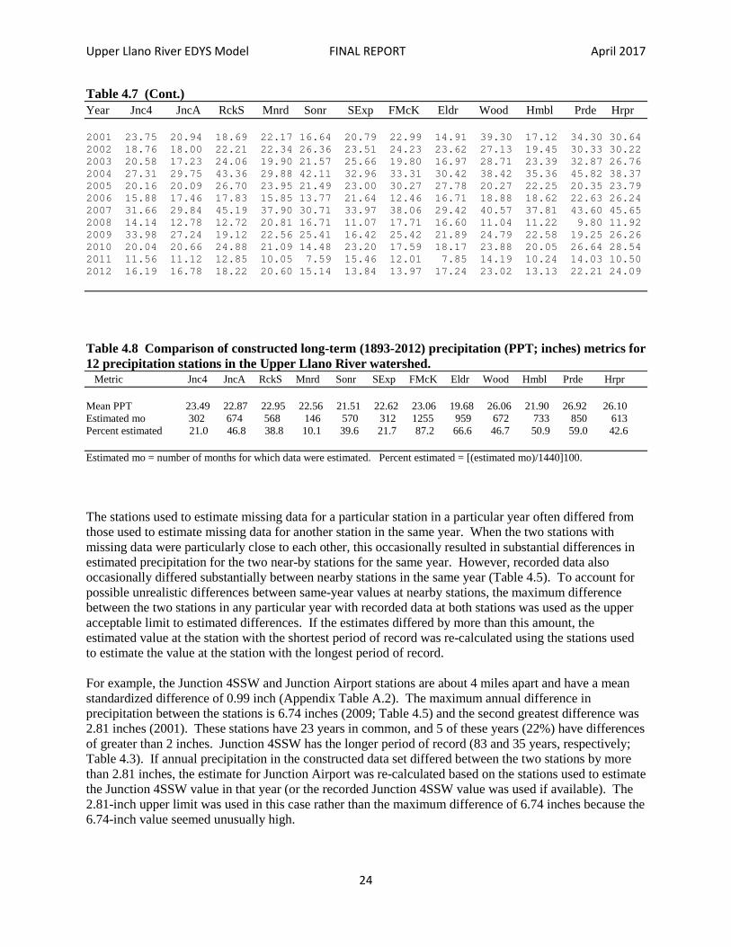
Upper Llano River EDYS Model FINAL REPORT April 2017
24
Table 4.7 (Cont.) Year Jnc4 JncA RckS Mnrd Sonr SExp FMcK Eldr Wood Hmbl Prde Hrpr 2001 23.75 20.94 18.69 22.17 16.64 20.79 22.99 14.91 39.30 17.12 34.30 30.64 2002 18.76 18.00 22.21 22.34 26.36 23.51 24.23 23.62 27.13 19.45 30.33 30.22 2003 20.58 17.23 24.06 19.90 21.57 25.66 19.80 16.97 28.71 23.39 32.87 26.76 2004 27.31 29.75 43.36 29.88 42.11 32.96 33.31 30.42 38.42 35.36 45.82 38.37 2005 20.16 20.09 26.70 23.95 21.49 23.00 30.27 27.78 20.27 22.25 20.35 23.79 2006 15.88 17.46 17.83 15.85 13.77 21.64 12.46 16.71 18.88 18.62 22.63 26.24 2007 31.66 29.84 45.19 37.90 30.71 33.97 38.06 29.42 40.57 37.81 43.60 45.65 2008 14.14 12.78 12.72 20.81 16.71 11.07 17.71 16.60 11.04 11.22 9.80 11.92 2009 33.98 27.24 19.12 22.56 25.41 16.42 25.42 21.89 24.79 22.58 19.25 26.26 2010 20.04 20.66 24.88 21.09 14.48 23.20 17.59 18.17 23.88 20.05 26.64 28.54 2011 11.56 11.12 12.85 10.05 7.59 15.46 12.01 7.85 14.19 10.24 14.03 10.50 2012 16.19 16.78 18.22 20.60 15.14 13.84 13.97 17.24 23.02 13.13 22.21 24.09 Table 4.8 Comparison of constructed long-term (1893-2012) precipitation (PPT; inches) metrics for 12 precipitation stations in the Upper Llano River watershed. Metric Jnc4 JncA RckS Mnrd Sonr SExp FMcK Eldr Wood Hmbl Prde Hrpr Mean PPT 23.49 22.87 22.95 22.56 21.51 22.62 23.06 19.68 26.06 21.90 26.92 26.10 Estimated mo 302 674 568 146 570 312 1255 959 672 733 850 613 Percent estimated 21.0 46.8 38.8 10.1 39.6 21.7 87.2 66.6 46.7 50.9 59.0 42.6 Estimated mo = number of months for which data were estimated. Percent estimated = [(estimated mo)/1440]100. The stations used to estimate missing data for a particular station in a particular year often differed from those used to estimate missing data for another station in the same year. When the two stations with missing data were particularly close to each other, this occasionally resulted in substantial differences in estimated precipitation for the two near-by stations for the same year. However, recorded data also occasionally differed substantially between nearby stations in the same year (Table 4.5). To account for possible unrealistic differences between same-year values at nearby stations, the maximum difference between the two stations in any particular year with recorded data at both stations was used as the upper acceptable limit to estimated differences. If the estimates differed by more than this amount, the estimated value at the station with the shortest period of record was re-calculated using the stations used to estimate the value at the station with the longest period of record. For example, the Junction 4SSW and Junction Airport stations are about 4 miles apart and have a mean standardized difference of 0.99 inch (Appendix Table A.2). The maximum annual difference in precipitation between the stations is 6.74 inches (2009; Table 4.5) and the second greatest difference was 2.81 inches (2001). These stations have 23 years in common, and 5 of these years (22%) have differences of greater than 2 inches. Junction 4SSW has the longer period of record (83 and 35 years, respectively; Table 4.3). If annual precipitation in the constructed data set differed between the two stations by more than 2.81 inches, the estimate for Junction Airport was re-calculated based on the stations used to estimate the Junction 4SSW value in that year (or the recorded Junction 4SSW value was used if available). The 2.81-inch upper limit was used in this case rather than the maximum difference of 6.74 inches because the 6.74-inch value seemed unusually high.

Upper Llano River EDYS Model FINAL REPORT April 2017
25
Based on recorded precipitation data (in contrast to constructed data), which do not include all of the same years or the same period of record, there is a decrease in average annual precipitation over the region from the southeast (wetter) to the northwest (drier)(Fig. 4.4). The constructed precipitation data are consistent with this regional pattern (Table 4.8).
Figure 4.4 Average annual precipitation pattern (inches) across the Edwards Plateau. Values are annual means based on recorded data for periods of record at each station. Periods of record and years with complete (12-month) data vary among stations. 4.4 Precipitation Regimes by Spatial Segment The constructed precipitation data (Table 4.7) were used to develop precipitation regimes for each of the seven segments of the spatial footprint. For each segment, an equation was developed (Table 4.9) based on the weighted average distances of each of the respective precipitation stations to the center of the segment. A long-term precipitation data set was calculated for each segment using these equations. The resulting seven long-term precipitation data sets were then entered into EDYS and used for model simulations.

Upper Llano River EDYS Model FINAL REPORT April 2017
26
Table 4.9 Equations used to calculate simulated precipitation events in each of the seven segments of the Upper Llano spatial footprint, based on constructed precipitation values for 12 precipitation stations (Table 4.8). NW Segment = 0.302(Humble Station) + 0.184(Sonora) + 0.166(Sonora Exp Sta) + 0.128(Fort McKavett) + 0.119(Eldorado) + 0.101(Junction 4SSW) NC Segment = 0.281(Humble Station) + 0.192(Junction 4SSW) + 0.167(Fort McKavett) + 0.140(Junction Airport) + 0.110(Menard) + 0.110(Rocksprings) NE Segment = 0.383(Junction 4SSW) + 0.206(Junction Airport) + 0.127(Fort McKavett) + 0.116(Humble Station) + 0.096(Menard) + 0.072(Rocksprings) Confluence = 0.520(Junction 4SSW) + 0.346(Junction Airport) + 0.035(Menard) + 0.035(Fort McKavett) + 0.033(Humble Station) + 0.031(Harper) SE Segment = 0.330(Junction 4SSW) + 0.198(Junction Airport) + 0.124(Humble Station) + 0.093(Prade Ranch) + 0.090(Rocksprings) + 0.085(Fort McKavett) + 0.080(Menard) SC Segment = 0.249(Humble Station) + 0.171(Rocksprings) + 0.140(Prade Ranch) + 0.140(Junction 4SSW) + 0.120(Junction Airport) + 0.095(Sonora Exp Sta) + 0.085(Camp Wood) SW Segment = 0.246(Humble Station) + 0.246(Rocksprings) + 0.139(Sonora Exp Sta) + 0.097(Sonora) + 0.097(Prade Ranch) + 0.091(Junction 4SSW) + 0.084(Camp Wood) 5.0 SOILS Two soil components are included in an EDYS model. First, a soils map is constructed that indicates the spatial location of each soil unit (soil series or soil type) included in the spatial footprint of the model. Second, profile descriptions are developed for each of the soil units. 5.1 Soils Map A total of 77 soil units were identified as occurring in the spatial domain of the Upper Llano model based on data from NRCS soil surveys for the respective counties (Blum 1982, Coffee 1967, Dittemore and Coburn 1986, Gabriel et al. 2009, Wiedenfeld 1980, Wiedenfeld and McAndrew 1968). Some of these soil units were similar to at least one other soil unit, differing in slope or relatively minor profile characteristics. To reduce the spatial complexity of the models, and thereby improve run times and reduce memory requirements, this group of 77 soil units was reduced to 48 for inclusion in the model (Table 5.1). The primary criteria used was whether or not the differences between the soil units were likely to result in measurable and ecologically significant differences in vegetation, hydrology, or management responses. The locations of each of these soils were mapped as soil polygons on the model spatial footprint (Fig. 5.1), and each 40 m x 40 m EDYS cell was assigned to one of the 48 soil units, based on the location of the cell in relation to the spatial distribution of the soil polygons.

Upper Llano River EDYS Model FINAL REPORT April 2017
27
Table 5.1 Soils included in the Upper Llano EDYS model. County Soil Symbol County Soil Symbol Edwards-Real Dev-Riverwash complex DeB Menard Dev Ds Edwards-Real Dina-Eckrant complex DnD Menard Kavett silty clay KaB Edwards-Real Eckrant-Rock outcrop 1-20% slope EcF Menard Tarrant Ta Edwards-Real Eckrant-Rock outcrop 20-50% slope EcG Menard Tarrant-Brackett association Tb Edwards-Real Ector gravelly silty clay loam ErB Menard Tobosa clay TsA Edwards-Real Irion clay IrA Menard Valera silty clay VaB Edwards-Real Leakey silty clay loam LkB Edwards-Real Oakalla-Dev complex OdA Edwards-Real Prade-Eckrant complex PeB Edwards-Real Rio Diablo silty clay RdB Kerr Denton silty clay DnB Schleicher Cho association 2 Kerr Eckrant-Rock outcrop ERG Schleicher Dev-Rioconcho association 3 Kerr Oakalla silty clay loam Oa Schleicher Kavett-Tarrant association 5 Kerr Purves-Tarrant association PTD Schleicher Tarrant association 8 Kerr Spires-Tarpley association STC Schleicher Tobosa clay 10 Kerr Tarrant-Eckrant association TTC Schleicher Valera-Mereta-Kavett 11 Kimble Cho gravelly loam CoC Sutton Caliche pits CLP Kimble Dev gravelly loam De Sutton Ector Es Kimble Frio silty clay loam Fr Sutton Frio-Dev association FD Kimble Gravel pit/Quarry GP Sutton Kavett-Tarrant complex Kt Kimble Kavett-Tarrant association KTB Sutton Angelo silty clay loam Ky Kimble Menard fine sandy loam MnB Sutton Reagan silty clay loam Rc Kimble Nuvalde clay loam, 1-3% slope NuB Sutton Tobosa clay Tc Kimble Oben-Hext complex OhC Sutton Tarrant-Rock outcrop complex Tr Kimble Real-Brackett complex, hilly RbF Sutton Tarrant Ts Kimble Tarrant, undulating TaC Kimble Tarrant-Rock outcrop TrG
Soils with the same name, but listed in multiple counties, have sufficiently different profiles to be modeled as separate soils.
Figure 5.1 Example of the spatial distribution of NRCS soil units on a portion of the Kimble County landscape. The four squares near the distance scale represent 40 m x 40 m plots.

Upper Llano River EDYS Model FINAL REPORT April 2017
28
5.2 Profile Descriptions A soil profile is a vertical section of a particular soil. Soils are composed of layers, called horizons, with each horizon differing in some major physical or chemical variable from the layer above and the layer below it. Horizons are designated by capital letters (e.g., A, B, C) in a top-down order. Horizons are often subdivided, and these subdivisions are designated by lower-case letters (e.g., Ap, Bk, Bt) the letters referring to specific types of soil conditions, and/or numbers (e.g., A1, A2, Bt1, Bt2), with the number indicating vertical order within the horizon (capital letter). General profile descriptions of each soil occurring in a particular county are provided in the NRCS Soil Survey for that county. An example, the Oben fine sandy loam, is presented in Table 5.2. Table 5.2 NRCS profile description of the Oben fine sandy loam in Kimble County (Blum 1982). Horizon Depth (cm) Texture Color Structure A1 00-15 fine sandy loam dark reddish brown weak fine subangular blocky B21t 15-30 sandy clay loam reddish brown weak medium subangular blocky B22t 30-48 sandy clay loam yellowish red weak medium subangular blocky R 48-63 limestone conglomerate yellowish red weakly to strongly cemented, fractured EDYS soil profiles are based on the NRCS profiles, but differ in two primary ways. First, the EDYS profiles contain more layers and extend to greater depths than their respective NRCS profiles. The usual time step in EDYS simulations is daily. Daily changes in belowground components that affect plant growth (e.g., available soil moisture, root growth, availability of soil nutrients) occur at finer spatial scales (soil depths) than those designated for NRCS soil horizons. For example, many precipitation events supply only small amounts of water. The median summer precipitation event in many semi-arid regions is less than 5 mm (Schwinning and Sala 2004). In many soils, a 5-mm rainfall event will supply water to only the top 5 cm of the soil profile and at that shallow depth will be rapidly extracted (two days, Sala and Lauenroth 1982) by evaporation before most of it can be used by plants in transpiration. In contrast, a 10-mm rainfall event on the same soil will supply some moisture to a depth of perhaps 10 cm and, at that depth, some of the water would be extracted by evaporation and some by transpiration. Only that water used in transpiration would be available to support plant growth. Therefore, small differences in soil depth can substantially affect plant growth responses. For this reason, thinner soil layers are used in EDYS. Each soil has a unique soil profile associated with it. Each EDYS profile in the Upper Llano model consists of 20 soil layers, with the thickness (depth) of each layer varying among soils. The 20 EDYS layers are subdivisions of the naturally occurring soil horizons. Soil horizons are subdivided into layers, but layers do not cross horizon boundaries. For example, no single EDYS layer would include the 25-35 cm depth of the Oben fine sandy loam (Table 5.2) because that would combine portions of different horizons. NRCS profile descriptions do not include the subsoil material. EDYS profiles extend much deeper than the NRCS profiles. Deeper soil layers (subsoil layers, beneath the soil profile) are added in EDYS to allow for deep drainage of water and penetration of deep-rooted species. Characteristics of these deep soil (parent material) layers are based on estimates of the characteristics of the parent material. These lower EDYS layers are thicker than the upper soil layers because daily changes in moisture inputs and root dynamics are not as dynamic as those in the upper layers and because less information is available relative to the characteristics of the lower layers. If the underlying material is rock, estimates are made of
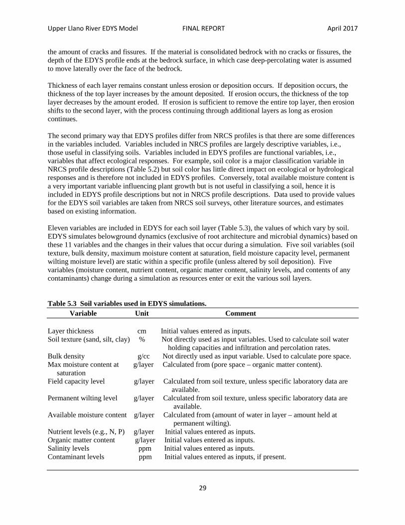
Upper Llano River EDYS Model FINAL REPORT April 2017
29
the amount of cracks and fissures. If the material is consolidated bedrock with no cracks or fissures, the depth of the EDYS profile ends at the bedrock surface, in which case deep-percolating water is assumed to move laterally over the face of the bedrock. Thickness of each layer remains constant unless erosion or deposition occurs. If deposition occurs, the thickness of the top layer increases by the amount deposited. If erosion occurs, the thickness of the top layer decreases by the amount eroded. If erosion is sufficient to remove the entire top layer, then erosion shifts to the second layer, with the process continuing through additional layers as long as erosion continues. The second primary way that EDYS profiles differ from NRCS profiles is that there are some differences in the variables included. Variables included in NRCS profiles are largely descriptive variables, i.e., those useful in classifying soils. Variables included in EDYS profiles are functional variables, i.e., variables that affect ecological responses. For example, soil color is a major classification variable in NRCS profile descriptions (Table 5.2) but soil color has little direct impact on ecological or hydrological responses and is therefore not included in EDYS profiles. Conversely, total available moisture content is a very important variable influencing plant growth but is not useful in classifying a soil, hence it is included in EDYS profile descriptions but not in NRCS profile descriptions. Data used to provide values for the EDYS soil variables are taken from NRCS soil surveys, other literature sources, and estimates based on existing information. Eleven variables are included in EDYS for each soil layer (Table 5.3), the values of which vary by soil. EDYS simulates belowground dynamics (exclusive of root architecture and microbial dynamics) based on these 11 variables and the changes in their values that occur during a simulation. Five soil variables (soil texture, bulk density, maximum moisture content at saturation, field moisture capacity level, permanent wilting moisture level) are static within a specific profile (unless altered by soil deposition). Five variables (moisture content, nutrient content, organic matter content, salinity levels, and contents of any contaminants) change during a simulation as resources enter or exit the various soil layers. Table 5.3 Soil variables used in EDYS simulations. Variable Unit Comment Layer thickness cm Initial values entered as inputs. Soil texture (sand, silt, clay) % Not directly used as input variables. Used to calculate soil water holding capacities and infiltration and percolation rates. Bulk density g/cc Not directly used as input variable. Used to calculate pore space. Max moisture content at g/layer Calculated from (pore space – organic matter content). saturation Field capacity level g/layer Calculated from soil texture, unless specific laboratory data are available. Permanent wilting level g/layer Calculated from soil texture, unless specific laboratory data are available. Available moisture content g/layer Calculated from (amount of water in layer – amount held at permanent wilting). Nutrient levels (e.g., N, P) g/layer Initial values entered as inputs. Organic matter content g/layer Initial values entered as inputs. Salinity levels ppm Initial values entered as inputs. Contaminant levels ppm Initial values entered as inputs, if present.

Upper Llano River EDYS Model FINAL REPORT April 2017
30
Three moisture level variables are utilized by EDYS: saturation, field capacity, and wilting (Table 5.4). The values entered for each of these variables is the level (% dry weight of soil) that corresponds to the upper limit for that condition in the soil of the particular soil layer. These values were determined using the NRCS soil moisture calculator (Saxton and Rawls 2006). The value for saturation corresponds to the maximum pore space for that layer (i.e., the water content at saturation). The field capacity value corresponds to the % water content at field capacity (~ -0.03 MPa). The difference between saturation and field capacity is drainage (gravitational) water. The value for wilting corresponds to the water content (%) at permanent wilting (~ -1.5 MPa). The difference between water held at field capacity and water held at permanent wilting is the amount of water available to plants. That difference, expressed as a percent, multiplied by the weight of the soil layer (bulk density x thickness of the layer) equals the available water content (g/m2; Table 5.4). Saturation capacity, field capacity, and wilting values are constant for a particular layer unless the texture or bulk density changes (by erosion or compaction). Available water content is a dynamic variable, i.e., its value changes during a simulation in response to precipitation, evaporation, and plant water uptake (transpiration). Table 5.4 Constructed EDYS soil profile data for the Denton silty clay soil, Upper Llano model. Layer Depth Thickness Bulk Soil Texture Organic Matter Nitrogen Moisture Level (%) Available (mm) (mm) Density Sand Silt Clay (%) (g/m2) (%) (g/m2) Saturation Field Wilting Water (g/cm3) (%) (%) (%) Capacity (g/m2) 01 00000-00025 0025 1.03 2 41 57 4.00 1,033 0.32 83 61.0 51.4 36.4 11.0 02 00025-00075 0050 1.22 2 41 57 3.00 1,824 0.24 147 54.1 50.8 35.8 21.7 03 00075-00125 0050 1.22 2 41 57 2.75 1,672 0.22 135 54.1 50.7 35.6 21.6 04 00125-00200 0075 1.22 2 41 57 2.00 1,824 0.16 147 54.1 50.2 35.2 32.0 05 00200-00300 0100 1.22 2 41 57 1.50 1,824 0.12 147 54.1 50.0 34.9 42.4 06 00300-00425 0125 1.28 30 33 37 1.00 1,599 0.08 129 51.7 35.1 21.1 35.2 07 00425-00550 0125 1.28 30 33 37 0.80 1,279 0.06 103 51.7 35.0 21.0 35.0 08 00550-00700 0150 1.28 30 33 37 0.60 1,151 0.05 93 51.7 34.9 20.9 41.8 09 00700-00875 0175 1.28 30 33 37 0.50 1,119 0.04 90 51.7 34.8 20.8 48.7 10 00875-01050 0175 1.46 46 24 30 0.40 1,020 0.03 82 45.0 25.7 15.4 35.9 11 01050-01250 0200 1.46 46 24 30 0.20 583 0.02 47 45.0 25.6 15.3 40.9 12 01250-01425 0175 1.46 30 20 50 0.01 26 0.001 2 24.7 15.0 10.0 21.9 13 01425-02000 0575 1.46 30 20 50 0.01 84 0.001 7 24.7 15.0 10.0 71.9 14 02000-04625 2625 1.46 30 20 50 0.01 382 0.001 31 24.7 15.0 10.0 328.4 15 04625-07250 2625 1.46 30 20 50 0.01 382 0.001 31 24.7 15.0 10.0 328.4 16 07250-09875 2625 1.46 30 20 50 0.01 382 0.001 31 24.7 15.0 10.0 328.4 17 09875-14375 4500 1.46 20 30 50 0.01 656 0.001 53 30.0 25.0 05.0 675.0 18 14375-18875 4500 1.46 20 30 50 0.01 656 0.001 53 30.0 25.0 05.0 675.0 19 18875-23375 4500 1.46 20 30 50 0.01 656 0.001 53 30.0 25.0 05.0 675.0 20 23375-28000 4625 1.46 20 30 50 0.01 674 0.001 54 30.0 25.0 05.0 694.8
Note: Denton silty clay typically has bedrock beginning at 125-150 cm. This corresponds to EDYS layers 12-20. The Table 5.4 values for those layers are for the soil in cracks in the limestone. For calculations of amounts, an assumption of 5% cracks by volume was made. Soil characteristic values for the soil in the cracks were estimated. Two other dynamic soil variables are included for each layer: organic matter and nitrogen content. An initial value for organic matter content (%) is included and EDYS then calculates the amount of organic matter (g/m2) contained in the particular layer. These values change during a simulation as organic matter is added (transport of litter, translocation of soil organic matter among layers, death of belowground plant and animal material) and lost (decomposition, translocation out of the layer). An initial value is also included for nitrogen (N), which is entered as % total N and is estimated as 1% of organic matter, unless soil specific data are available. The value for total N changes during a simulation, based on input of N into the top layer from precipitation, release of N during mineralization of organic matter, transport of N into and out of the layer, and plant and microbial uptake of available N. Available N is calculated by
Upper Llano River EDYS Model FINAL REPORT April 2017
31
EDYS as 1% of total N (4%; Paschke et al. 2000), and this calculation is made on a daily time step, based on rate of mineralization. Water is a major factor controlling both above- and belowground dynamics. Terrestrial plants uptake the water they need for maintenance and growth from the soil (including groundwater in the subsoil). The location (depth) of water stored in the soil (i.e., soil moisture) in relation to root architecture of the various plant species is an important factor controlling the competition among these species. Nutrients and contaminants become available for plant uptake as they enter into soil solution and their concentrations vary as amounts are moved among layers by water movement. Organic matter is also moved among layers by water movement and the decomposition and mineralization rates of organic matter are controlled, in part, by the moisture content of the soil. In EDYS, water can arrive at the surface layer of a spatial cell in two ways, by a precipitation event and by surface movement from adjacent cells (i.e., run-on). Some of this water can enter the soil profile (infiltration) and some exits the cell as runoff. Litter on the soil surface has first opportunity for absorption of water in EDYS. If litter is present and is at less than its maximum moisture content, it can absorb sufficient water to bring it up to maximum moisture content. The remaining water is available for infiltration into the soil profile and runoff from the cell. In EDYS, the amount of water that can potentially enter into the soil profile during a rainfall event is modeled as a step function. The amount of rain in each daily rainfall event is divided into five parts (10%, 20%, 40%, 20%, and 10% of the total amount). The amount of water in Step 1 (10% of the rainfall event) is compared to the available storage capacity (saturation capacity minus current moisture content) of the first layer. If the amount of water is less than or equal to the available storage capacity, that entire quantity of water (10% of the event) is moved into the first layer. If the amount is in excess of available storage capacity, the excess amount is moved to adjacent cells as runoff. This process is repeated through each of the next four steps, with number of layers used to calculate available storage capacity increasing by one layer at each step (e.g., Step 3 = 40% of rainfall event compared to available storage capacity of top three layers). Once water moves into a soil layer, it is moved downward using a “tipping bucket” algorithm. Any water in excess of field capacity of the first layer moves into the second layer. Any water in excess of field capacity for that layer is moved into the third soil layer. This process continues in a top-down manner until the all of the water is stored in the various soil layers, or if some remains once the wetting front reaches saturated soil (groundwater), the surplus amount is added to groundwater. If the groundwater is unconstrained (i.e., groundwater lateral flow can occur), this amount of added water is removed as “export”. If the groundwater is constrained, then the water content of the layer immediately above the saturated layer increases above field capacity. This increase can continue until the saturation level is reached for that layer, at which time the process continues in an upward manner into the next unsaturated layer. As water moves downward by percolation (or upward by saturation or capillarity), soluble materials (nutrients, contaminants, organic matter) can be moved with the water. As water moves into the next layer at each time step, the concentrations of the soluble materials in that layer are recalculated based on the amount of those materials in the layer prior to entry of the new water and the new concentration resulting from all the surplus water (not just field capacity) that at least temporarily moves into that layer. Then if some water continues to move downward out of that layer, that water transports with it the amount of nutrients, contaminants, and organic matter corresponding to its relative concentration. Soil water (including groundwater) is extracted from each layer at each time step by plant uptake (transpiration). The amount removed from each layer is determined by the amount of roots of each plant

Upper Llano River EDYS Model FINAL REPORT April 2017
32
species in that layer, the depth of the layer (root uptake is modeled as a top-down process), and the amount of water transpired by each species. Soil water can also be extracted by evaporation. However, evaporation occurs directly only from the surface soil layer. Stored soil moisture can be moved from upward to the surface soil layer (capillarity) and then lost to evaporation, but only from a maximum of the next three soil layers. This is a time-step controlled process and plant roots get first priority use of the water as it moves upward form the second, third, and fourth soil layers. In addition to movement by water, organic matter can be added to a soil layer by death of plant material (roots) in that particular layer and by some movement of surface litter into the upper soil layer. The deposition of this material is based on root death rates specific to each species and decomposition rates that are influenced by moisture content and nitrogen availability. 6.0 VEGETATION An EDYS application utilizes two broad types of plant data: parameter data for individual plant species and data on the composition of vegetation communities. 6.1 Selection of Plant Species The number of plant species included in a specific EDYS application is flexible. How many and which species to be included depends on the requirements of the application and the level of complexity desired. The inclusion of more species increases the potential for the model to simulate the complexity common to most landscapes, but it also increases run times and memory requirements. The EDYS data-base contains ecological data on over 250 species, not all of which occur in the western Edwards Plateau and not all of which have data for all plant parameter variables used in EDYS. In each EDYS application, a subset of all species occurring in the spatial domain is used. Several factors are considered in the selection of this subset.
• The subset should include the major species for the area, based on both ecological and management importance. Ecological importance includes dominant and sub-dominant species for each of the included plant communities, species important successionally, any threatened and endangered species, and any major invasive species or other species of concern.
• There must be sufficient ecological data available for the included species that the required parameter variable values can be determined or reasonably estimated. Data for all parameter variables may not be available for a major species. In such cases, reasonable estimates can often be made based on available data for closely-related or ecologically-similar species.
• For species where a substantial amount of their parameter values are estimated, care must be taken that the estimates are not based largely on data from species used to estimate values for other included species. Otherwise, little new information is actually included in the model by adding another species.
• The inclusion of the species should be expected to sufficiently increase the ability of the model to simulate ecological responses to justify any associated increase in run time, memory requirements, or time required to interpret results.

Upper Llano River EDYS Model FINAL REPORT April 2017
33
• The inclusion of the species should not unduly increase unaccounted error (i.e., “noise”) into the
model output.
Based on the factors listed above, 51 species were included (Table 6.1). Table 6.1 Plant species (51) included in the Upper Llano River EDYS model. Lifeform Species Common Name Trees (7) Carya illinioensis pecan Celtis laevigata sugar hackberry Diospyros texana Texas persimmon Juniperus ashei Ashe juniper Prosopis glandulosa mesquite Quercus buckleyi Texas red oak Quercus virginiana live oak Vines (1) Vitis mustangensis mustang grape Shrubs (6) Baccharis texana prairie baccharis Forestiera pubescens elbowbush Mahonia trifoliolata agarito Nolina texana sacahuista Rhus virens evergreen sumac Yucca constricta yucca Succulents (1) Opuntia lindheimeri Texas prickly pear Grasses (22) Arundo donax giant cane Aristida purpurea purple threeawn Bothriochloa barbinodis cane bluestem Bothriochloa ischaemum King Ranch bluestem Bouteloua curtipendula sideoats grama Bouteloua hirsuta hairy grama Bouteloua trifida red grama Cynodon dactylon bermudagrass Elymus canadensis Canada wildrye Eragrostis intermedia plains lovegrass Eriochloa sericea Texas cupgrass Hilaria belangeri curly mesquite Leptochloa dubia green sprangletop Panicum obtusum vine-mesquite Panicum virgatum switchgrass Schizachyrium scoparium little bluestem Sorghastrum nutans indiangrass Sorghum halepense Johnsongrass Sporobolus asper tall dropseed Sporobolus cryptandrus sand dropseed Stipa leucotricha Texas wintergrass

Upper Llano River EDYS Model FINAL REPORT April 2017
34
Table 6.1 (Cont.) Lifeform Species Common name Triticum aestivum wheat Grass-Likes (4) Cyperus odoratus flatsedge Eleocharis palustris spikerush Scirpus acutus bulrush Typha latifolia cattail Forbs (10) Ambrosia psilostachya ragweed Aphanostephus ramossissimus lazydaisy Desmanthus velutinus bundleflower Gaillardia pulchella Indian blanket Helianthus annuus sunflower Lemna minor duckweed Lupinus texensis Texas bluebonnet Ratibida columnifera prairie coneflower Simsia calva bush sunflower Zexmenia hispida orange zexmenia 6.2 Plant Parameter Variables EDYS is a mechanistic model. It simulates ecological dynamics by modeling how the various ecological components function. For plants, this is accomplished by using mathematical algorithms to model how plants grow and respond to various environmental stressors, such as drought, fire, and herbivory. There is a large number of algorithms associated with plant dynamics in the EDYS model (Childress et al. 1999b; Coldren et al. 2011a). Each algorithm is applied to each plant species at each time step during a simulation to simulate the change in that plant or plant part from one time-step to the next. Each algorithm contains 1-6 plant response variables (parameters). Differential responses among plant species are achieved in EDYS by assigning species-specific values to each of these plant parameters. For example, one of the algorithms is plant growth, more specifically, increase in plant biomass. This algorithm contains a number of parameters, one of which is “water to production”. This parameter (water to production) is the amount of water (in kilograms) required to produce one gram (dry-weight) of new plant biomass and it is species specific (i.e., the water-use efficiency varies by species). Two of the major perennial grasses in the Upper Llano model are little bluestem (Schizachyrium scoparium) and curly mesquite (Hilaria belangeri). The water-to-production value for little bluestem is 0.90 and the value for curly mesquite is 0.65. Curly mesquite is the more xeric of the two grasses and indeed has the higher water-use efficiency. There are 346 plant parameter variables in EDYS and each one of these has a specific value for each species in an application (51 species in the case of the Upper Llano model). These variables are arranged into 40 plant parameter matrices (Table 6.2). The data are entered from the EDYS Data Base, which contains values collected from the scientific literature and from field and greenhouse studies conducted as parts of previous EDYS applications. Values for selected plant parameter matrices and sources of these data are presented in Appendix C. If species-specific data are not available for a particular species for

Upper Llano River EDYS Model FINAL REPORT April 2017
35
one or more of the plant parameter values, estimates are made based on data on most-similar (ecologic or taxonomic) species. Table 6.2 List of plant parameter matrices used in EDYS applications. Matrix Variables 01 General lifeform growth form, lifespan, legume or not 02 Tissue allocation (mature) proportion of coarse roots, fine roots, trunk, stems, leaves, seeds; root:shoot ratio 03 Tissue allocation (new) proportion of new production allocated to each plant part 04 Tissue allocation (green-out) proportion of new production allocated to each plant part during green-out 05 Tissue allocation (seed mo) proportion of new production allocated to each plant part during flowering 06 Tissue N concentration nitrogen concentration of each plant part 07 Required N concentration minimum nitrogen concentration of each plant part 08 Nitrogen resporption proportion of current nitrogen concentration that is resorbted at dormancy 09 Root architecture root distribution by depth for each species; maximum potential rooting depth 10 Root uptake & competition uptake capacity, growth rate, saturation death loss, fine:coarse roots at dormancy 11 Physiological response months when green-out, dormancy, seed set, and seed germination occur 12 Biomass conversion factors moisture content, canopy interception rate, basal cover:trunk biomass ratio 13 Water-use factors maintenance requirement (old, new biomass), water-use efficiency, green-out 14 Growth rate controls maximum monthly growth rate, max aboveground biomass, max drought loss 15 Monthly growth rates proportion of maximum monthly growth rate each species can have in each month 16 Plant part productivity potential photosynthetic rate of each plant part 17 Green-out production amount of biomass in each plant part converted to new-production at green-out 18 Physiological controls maximum root:shoot ratios; seed germination rate; seedling growth rate 19 Dormancy dieback proportion of each plant part lost (annual) during dormancy 20 Shading effect reduction in production in each species by shading from each other species 21 Dieback fate where dead plant biomass, by plant part, is located following death 22 Groundwater response amount of water that can potentially be extracted by soil depth, by species 23 Flooding effects maximum number of days species can tolerate flooding 24 Salinity effects salinity levels at which growth is reduced (reduction = 0%, 50%, 100%) 25 Fuel load contribution heat load factor for each plant part, by species 26 Plant loss to fire proportion of plant part, by species, lost to a moderate-intensity fire 27 Vehicle impacts proportion of plant part, by species, lost to a single pass of a standard vehicle 28 Foot traffic impacts proportion of plant part, by species, lost to a single step of a human 29 Cattle preference selection of plant parts by species by cattle 30 Cattle competition rank of cattle among all herbivores in ability to consume plant parts by species 31 Cattle accessibility amount of each plant part, by species, that can be consumed by cattle 32 Deer preference selection of plant parts by species by white-tailed deer 33 Deer competition rank of white-tailed deer among all herbivores in ability to consume plant parts 34 Deer accessibility amount of each plant part, by species, that can be consumed by white-tailed deer 35 Rabbit preference selection of plant parts by species by rabbits 36 Rabbit competition rank of rabbits among all herbivores in ability to consume plant parts 37 Rabbit accessibility amount of plant part, by species, that can be consumed by rabbits 38 Insect preference selection of plant parts by species by insects (grasshoppers) 39 Insect competition rank of insects (grasshoppers) among all herbivores in ability to consume plants 40 Insect accessibility amount of plant part, by species, that can be consumed by insects (grasshoppers) General characteristics of each species are presented in Matrix 01. Matrices 02-05 are the tissue allocation matrices. At each time-step, EDYS calculates the amount of new biomass produced by each species. This amount is based on 1) amount of current photosynthetically active biomass, 2) potential growth rate, and 3) amount of required resources available to the species (function of amount of each resource available in the rooting zone and the competitive ability of the specific species to secure this

Upper Llano River EDYS Model FINAL REPORT April 2017
36
resource). The amount of new biomass produced by each species is then allocated to the various plant parts based on the values in the allocation matrices.
Matrix 02 provides the information that EDYS uses to allocate the beginning biomass values (Appendix Tables B.1-3) to the various plant parts to begin a simulation. During a simulation, new biomass production is allocated during each time-step to the various plant parts based on the values in Matrix 03. For example, if 10 g of new biomass is produced by Ashe juniper, 0.8 g would be added to coarse roots, 3.0 g would be added to fine roots, 1.1 g would be added to trunk, 2.0 g would be added to stems, and 3.1 g would be added to leaves (Appendix Table C.3). These ratios are used throughout the growing season, except in months when the species flowers or undergoes green-out. Green-out occurs following winter dormancy, drought dormancy, or following severe defoliation. For months when green-out occurs, the values from Matrix 04 are used instead of those from Matrix 03, and for months for seed-set (flowering) the values from Matrix 05 are used.
Root architecture varies substantially among plant species and these variations are important in determining competitive responses among species for belowground resources (e.g., water and nutrients). Two components of root architecture of primary importance are distribution of roots by soil depth and maximum potential rooting depth. Matrix 09 provides the values for these two parameters for each of the species in the model. These values are used in EDYS to determine the initial spatial distribution of root biomass.
The amount of roots for a particular species at the beginning of a simulation is determined by multiplying the coarse and fine root allocation values (Matrix 02) by the initial biomass value for that species in a given plot type (Appendix Tables B.1-3). The values in Matrix 09 are then used to allocate this root biomass (coarse and fine) by soil depth. This is calculated as the product of:
(total root biomass)(% in a portion of the rooting depth)(maximum potential rooting depth).
For example, 1% of the roots of Ashe juniper are assumed to be located in the first 1% of the rooting depth of Ashe juniper (Appendix Table C.9). The maximum reported rooting depth of Ashe juniper is 8 m (Jackson et al. 1999), therefore 1% of the initial root biomass of Ashe juniper is located in the upper 80 mm (3.1 inches) of the soil. If the maximum depth of a soil in a particular plot types is less than the maximum potential rooting depth, the maximum soil depth is used instead. The values in Matrix 09 are used to calculate the initial distribution of roots in an EDYS simulation. At each time-step during a simulation, new root biomass is added (e.g., Matrix 03). This new root biomass is added to the current root biomass in those soil depths where active root uptake of water and nutrients are taking place. This results in potential changes in root distribution during a simulation caused by resource distribution. Matrix 11 provides values used to determine when specified physiological processes occur. These processes are 1) green-out (breaking of winter dormancy), 2) beginning of winter dormancy, 3) months in which flowering and seed production can occur, and 4) months in which seed germination can occur. Matrix 13 provides values used to determine water requirements of each species for maintenance and production of new biomass. Maintenance water requirements (old and new growth) refer to the amount of water used each month to support existing biomass. Water to production is the amount of water required to produce 1 g (dry-weight) of new biomass (i.e., water-use efficiency). Green-out water requirement is the amount of water required to support the production of new biomass during green-out. At each time-step during the growing season for a particular species (Matrix 11), EDYS calculates the amount of water that species would require if it produced at its maximum potential rate (Matrix 14) plus

Upper Llano River EDYS Model FINAL REPORT April 2017
37
the amount required to maintain existing tissue. EDYS then calculates how much soil moisture is available to that species at that time-step, as determined by the distribution of moisture in the soil at that time and the competition for that water among all species with roots in each particular soil layer. If the amount of water available is equal to or greater than the amount required, the plant produces that much new biomass and that quantity of water is removed from the respective soil layers. If the amount of water available to the species is less than the amount required, maintenance requirements are met first and any remaining water is used to produce new biomass, the amount of which is proportional to what can be produced on the remaining amount of water (water to production). EDYS also determines nutrient requirements in a manner similar to water requirements (Matrix 07). If nutrients are more limiting to plant growth than water requirements at that time-step, the amount of new growth produced is determined by the amount of nutrients available rather than the amount of water available, and the amount of water used is reduced proportionately. Matrix 14 provides values used to determine maximum potential growth rate, maximum size of the plants, and the maximum rate of tissue loss from drought. Maximum potential growth rate is the maximum rate that new biomass can be produced under optimum conditions for that species. Maximum potential growth rate is genetically determined for each species. Actual growth rate is most often less than this value because of resource limitations and tissue loss (e.g., herbivory, trampling). The values in Matrix 14 are multiplied by the amount of photosynthetically-active tissue (Matrix 16) present in that species at that time-step. The product is the maximum amount of new tissue that species can produce in that particular month. The actual amount produced is generally less than this maximum amount, based on resource limitations (water, nutrients, light, temperature). Maximum aboveground biomass is the maximum amount of standing crop biomass (g/m2) that is possible for that species. This variable limits the accumulation of biomass to realistic levels for each species. Maximum old biomass drought loss is the maximum amount (proportion of existing biomass) that can be lost in one month from drought. Matrix 15 provides a seasonal growth function for each species. A value of 1.00 indicates that the species can potentially grow at its maximum rate (Matrix 14) during that month. Values less than 1.00 result in proportional decreases in the maximum potential growth rate during those months. The values in Matrix 14 are estimates based on responses to both temperature and photoperiod. Maximum potential growth rates (Matrix 14) are based on photosynthetically-active tissue. For most species, the tissue with the highest potential photosynthetic rate are leaves. Cacti are an exception. Cacti leaves are their thorns. Stems and pads are the photosynthetically-active tissue in cacti. Roots and trunks of most species are structural tissues and do not contribute directly to photosynthesis, although there are exceptions (e.g., trunks or retama and paloverde trees). Stems of many species contribute somewhat to photosynthesis, but generally at a lower rate than leaves. Matrix 16 provides values for the photosynthetic potential of each plant part for each species. The values are proportions of maximum rates for that species (leaves for most species). Green-out in plants, whether as spring green-up or recovery from defoliation, requires an energy source. Carbohydrates stored in various tissues are used to produce the new biomass. Some storage is in areas near the meristematic regions (e.g., bud zones) whereas other storage is in more distant tissues (e.g., coarse roots, bases of trunks) and must be translocated to the points of new growth. In both cases, there is a loss of biomass (weight) in some tissue because of the loss of stored carbohydrates. Matrix 17 provides values used to determine how much current biomass (stored carbohydrates) can be used to produce new tissue during green-out. A value of 1.00 indicates (Appendix Table C.17) that the amount of tissue in that plant part can be doubled during a green-out month. A value of 0.10 indicates that 10% of the biomass in

Upper Llano River EDYS Model FINAL REPORT April 2017
38
that plant part can be transformed into new biomass during one month of green-out. During a green-out month, that amount of biomass is removed from the supplying plant part and transferred to new biomass and allocated according to the ratios in Matrix 04. Matrix 18 contains values for four physiological control variables. These variables are used in EDYS to assure that plant structure does not become unbalanced and that the conversion from seeds to new plant biomass occurs properly. Each species has a characteristic root:shoot ratio (Matrix 02). This is the relative amount of roots and shoots for that species. However, these ratios change during the growing season as new aboveground biomass is added and over years as perennial tissues accumulate belowground. Growing season maximum root:shoot ratio is a control to keep too much root biomass from accumulating over time. If this value is exceeded during a growing season, no new biomass is allocated to roots until the value drops below this maximum value. Growing season green-out shoot:root ratio has a similar function. Maximum 1-month seed germination limits the amount of the seed bank that can germinate in any one month. Maximum first-month seedling growth provides the value to convert germinated seed biomass to new plant biomass. The amount of germinated seed biomass is multiplied by this value and the product becomes new plant tissue for that species. At the end of the growing season plants enter winter dormancy (or summer dormancy for cool-season species) and loose some of their tissue (Matrix 11). An obvious example is deciduous trees shedding their leaves in the fall. But other tissue losses also occur. Some stems die. There can be some loss of trunk biomass. Root death occurs. Matrix 19 provides the values used to calculate these losses. A major factor in competition among plant species in many areas is shading, i.e., competition for light. Tall plants have a shading effect on shorter plants. Matrix 20 provides for this competitive response. The values listed are reductions in maximum potential growth rate of the shaded species that would result from 100% canopy cover of the shading species. The values in Matrix 20 (Appendix Table C.20) do not represent the entire competitive effect of overstory species on understory species, only the direct effect of shading. Overstory species also affect the growth of understory species in other ways, e.g., competition for moisture and nutrients. Those competitive effects are simulated in EDYS using other parameters. The shading parameter only reflects competition for light. In EDYS, values are averaged within a cell (Section 2.0), which are 40 m x 40 m on the uplands in the Upper Llano model. Within each cell, estimates are made of the amount of woody plant cover (e.g., 10-25%) based on aerial photographs (Section 6.3.1). A 25% cover of woody plants could result from various combinations of clusters (mottes) of trees and shrubs. In effect, the cell would consist of at least two vegetation types, one associated with the woody-species clusters and distributed over 25% of the surface of the cell and the other associated with herbaceous vegetation in the interspaces and distributed over the remaining 75% of the cell. However, the EDYS routine is to average the two types across the cell because the cell is the smallest subdivision in an EDYS application. In effect, this reduces the size of the woody plants (25% of the actual size in this example) and assumes that biomass is average (uniform) across the cell. If the shading factor is ignored, this averaging does not substantially alter the vegetation and hydrologic dynamics of the cell. With shading, the effect is to reduce herbaceous understory vegetation across the entire cell instead of just under the woody-plant clusters which should cover only 25% of the cell. An update is being developed that will account for this spatial heterogeneity within a cell. That update is not complete and therefore was not included in the Upper Llano model. Instead, the shading factor was utilized to simulate the effect of woody species on other woody species (i.e., under the woody plant canopy) and not for the shading effect of woody species on herbaceous species. The shading factor was also used to simulate the shading effect of herbaceous species on other herbaceous species (e.g., midgrasses shading shortgrasses). This dual-component approach allows dynamics of herbaceous species

Upper Llano River EDYS Model FINAL REPORT April 2017
39
to be simulated in the portion not covered by woody species, while maintaining the major aspect of shading within the area covered by woody plants. This dual pattern is a major characteristic of shrub and woodland mosaics, which have little herbaceous vegetation under dense woody canopies but relatively abundant grasses and forbs in the interspaces (Drawe et al. 1978; McLendon 1991). In addition, reduction in herbaceous species under woody plant canopies may not occur until cover of woody species increases above 30-50% (Scifres et al. 1982; Fuhlendorf et al. 1997). Plants can utilize groundwater when it, or its capillary fringe, is within their rooting zones. Although this is a potential source of water to plants, its actual contribution depends on the plant species, depth to groundwater (DTW), and availability of soil moisture. Soil water extraction by plants can be viewed in terms of the amount of energy required to access and move the water (Gardner 1991; Adiku et al. 2000). As a result, most species tend to utilize soil moisture in upper soil zones (if it is available) rather than groundwater, even when their roots are in contact with groundwater. However, there are often substantial differences in relative amounts of deep soil moisture and groundwater used by various species, even among the same lifeforms (e.g., trees, shrubs) when growing at the same locations (Flanagan and Ehleringer 1991; Donovan and Ehleringer 1994; Cook and O’Grady 2006). Matrix 22 provides values used in EDYS to adjust groundwater usage by depth and by species. Two vegetation components that are important in determining the impact of fire on vegetation are fuel load and susceptibility of species and plant parts to fire. Matrix 25 provides values for relative fuel load for each plant part. Factors included are size (e.g., fine fuel, wood), moisture content, and presence of oils in the tissue. Matrix 26 provides values used to determine sensitively of various plant parts and species to fire and various intensities determined by fuel load (Matrix 25). Herbivory is a major factor influencing vegetation dynamics. These effects are simulated in EDYS differentially by animal species on the various plant species. These parameters are provided in Matrices 29-40, and are discussed in more detail in Section 7. 6.3 Plant Communities In EDYS, each cell is assigned an initial vegetation composition based on some combination of the plant species included in application (Table 6.1). Because actual species composition data are not available for each cell in the spatial footprint, initial vegetation assignments are made on the basis of plant communities. A vegetation map is prepared by dividing the spatial footprint into polygons, each polygon representing a localized occurrence of a particular plant community or land-use type (e.g., cultivated field, lake/pond, roadway, caliche/gravel pit, building). If detailed vegetation maps are available, the polygons are assigned to specific plant communities based on the site-specific information (e.g., McLendon et al. 2010, 2013). Most often, as was the case for the Upper Llano River model, these detailed vegetation maps are not available. In these cases, a first-approximation classification of the polygons is made using the soil maps from the NRCS soil surveys (Coffee 1967; Wiedenfeld and McAndrew 1968; Wiedenfeld 1980; Blum 1982; Dittemore and Coburn 1986; Gabriel et al. 2009) along with their associated ecological sites (range site descriptions in earlier soil surveys). This provides the preliminary vegetation map. Each 40 m x 40 cm cell is then assigned to its respective vegetation type based on its spatial location on the landscape. 6.3.1 Terrestrial Vegetation The initial definitions of the plant communities (species composition and biomass values) are based on NRCS range or ecological site descriptions. These NRCS descriptions are then modified based on information from published scientific references, unpublished field studies, and professional judgment. A common modification relates to successional stage (range condition) of the plant community. The NRCS

Upper Llano River EDYS Model FINAL REPORT April 2017
40
site descriptions are based primarily on estimated potential late-successional conditions (excellent range condition). Most ranges are in earlier successional stages, with species composition and productivity levels different from those listed in the site descriptions. In addition, the NRCS site descriptions need to be modified to account for increased cover of woody plants. The NRCS site descriptions assume a relatively low amount of woody plant cover under late successional conditions. For example, the 13 range sites described for Kimble County have an average woody plant cover of 11% (Blum 1982). Most of the native rangeland in Kimble County has more than 11% cover of woody species. To account for woody plant cover, the vegetation polygons were superimposed on 2012 NAIP aerial photographs and the amount of woody plant coverage in each polygon was visually estimated. If there are substantially different amounts of woody plant coverage in different parts of the polygon, the polygon was subdivided on the basis of amount of woody plant coverage. Each subdivision is then assigned a different variation of the plant community, each variation having a species composition and productivity reflecting its level of woody plant coverage. In general, current vegetation conditions have more woody plants, more shortgrasses, less midgrasses, and lower herbaceous productivity than under late-successional conditions (Table 6.3). Based on data from the NRCS soil surveys (Coffee 1967, Wiedenfeld and McAndrew 1968, Wiedenfeld 1980, Blum 1982, Dittemore and Coburn 1986, Gabriel et al. 2009) and published research data (Reardon and Merrill 1976, Smeins et al. 1976, McGinty et al. 1979, Taylor et al. 1980, Shaw and Smeins 1983, McCalla et al. 1984, Thurow et al. 1986, Ralphs et al. 1990, Fuhlendorf et al. 1997, Wu et al. 2001), adjustments were made to account for earlier successional conditions in herbaceous composition. An example for the stony hill range site is provided in Table 6.4. The values in Table 6.4 assume average precipitation. EDYS accounts for variations in precipitation by adjusting the productivity of each species relative to precipitation received and competition for this moisture among the species present (herbaceous and woody). Table 6.3 Comparison of species composition on a low stony hill range site in Sutton County based on NRCS soil survey (Wiedenfeld and McAndrew 1968) and research data from the Sonora Experiment Station (Smeins et al. 1976, McGinty et al., 1979, Taylor et al. 1980, Ralphs et al. 1990). NRCS Soil Survey Average forage production = 275 g/m2 (2500 lbs/acre) Average woody plant cover = 15% Major forage species: sideoats grama, silver bluestem, little bluestem, green sprangletop, plains lovegrass, Texas wintergrass, plains bristlegrass, tall dropseed, Neally grama, Canada wildrye, vine-mesquite, indiangrass Sonora Experiment Station Average forage production = 148 g/m2 (1300 lbs/acre) Average woody plant cover = 18% Major forage species: curly mesquite, sideoats, threeawns, hairy tridens, Texas wintergrass, Texas cupgrass, Caucasian bluestem, red grama, hairy grama, cane bluestem, fall witchgrass, King Ranch bluestem Both sites have Tarrant and Ector soils.

Upper Llano River EDYS Model FINAL REPORT April 2017
41
Table 6.4 Estimated aboveground clippable biomass (g/m2) in grassland openings on low stony hill range sites in Edwards, Kimble, and Sutton Counties, Texas, in years of average precipitation, under each of four range condition classes. Species Range Condition Class Excellent Good Fair Poor Curly mesquite 70 80 40 30 Sideoats grama 30 30 5 2 Texas wintergrass 20 20 15 10 Cane bluestem 15 10 1 0 Purple threeawn 10 20 20 10 Hairy grama 10 15 20 5 Texas cupgrass 10 10 1 0 King Ranch bluestem 5 10 15 20 Red grama 0 5 10 10 Indian blanket 10 7 3 1 Orange zexmenia 8 5 2 1 Lazydaisy 5 3 1 1 Bundleflower 5 3 1 0 Prairie coneflower 2 1 1 0 Ragweed 0 1 5 10 Total herbaceous 200 220 140 100 Initial species composition values are entered into EDYS to begin a simulation. Initially, all cells in a particular plant community are given the same species composition. Although each cell in a vegetation polygon (initial plant community) has the same initial species composition, it does not necessarily remain the same during a simulation. Once the simulation begins, composition can change in response to the ecological dynamics that occur during the simulation. Differences in topographic features, precipitation zones and depths to groundwater, natural disturbances (e.g., fire), and management impacts (e.g., livestock grazing intensity, reseeding, brush control) often result in some cells within an initial vegetation community changing sufficiently that they form a separate vegetation type. Initial species composition values were calculated for each soil type, based on the plant community assigned to that soil type, assuming fair range condition (Appendix Tables B.1-B.3). In addition to literature data and aerial photographs, limited ground truthing of the vegetation maps was conducted, primarily along the rivers. Some field sampling was also conducted in Kimble County to investigate the spatial distribution of herbaceous vegetation in juniper communities. Should more site-specific information on range condition or species composition become available, these values can be changed for the appropriate polygons. In addition to successional stage of the herbaceous vegetation, adjustments were made to account for woody plant coverage. As woody plant cover increases, there is a shift is species composition of the woody species and a decrease in herbaceous production. On the low stony hill range site for example, the increase in woody plant cover comes primarily from an increase in Ashe juniper and live oak, with Ashe juniper increasing more than live oak (Table 6.5). At 15% woody plant cover, the site might be in good range condition with herbaceous production at about 90% of what it would be in a pure grassland (Table 6.5). As woody cover increases, both range condition and herbaceous production decrease. With 90% cover of woody plants range condition would be poor and herbaceous production low (15% of potential

Upper Llano River EDYS Model FINAL REPORT April 2017
42
production under poor condition without woody plants; Table 6.5). Species composition of the woody plant community also varies with plant community (Appendix Tables B.5-B.7). Table 6.5 Species composition (% absolute cover) and herbaceous production (% of pure grassland at same range condition class) on wooded low stony hill range sites in Edwards, Kimble, and Sutton Counties, Texas. Species Woody Plant Cover 15% 25% 35% 90% Ashe juniper 5 9 10 45 Live oak 5 9 10 27 Mesquite 1 1 1 1 Texas persimmon 1 2 3 1 Elbowbush 1 1 1 <0.1 Agarito 1 1 1 <0.1 Prickly pear 1 1 1 <0.1 Herbaceous 90% of 80% of 70% of 15% of good fair fair poor condition condition condition condition Sufficient field data are not available to account for this effect of woody plant cover on productivity and composition of the herbaceous understory. As a first-approximation estimator, composition is addressed in this version of the Upper Llano model by assuming the plant communities are in fair range condition (Appendix Tables B.1-B.3) rather than in excellent condition as presented in the NRSC Soil Surveys. The values listed in Appendix Tables B.1-B.3 are for fair condition with no woody plant cover. To account for the effect of woody plant cover on herbaceous productivity, these values (by species) were adjusted by the formula (Appendix Table B.12): herbaceous biomassw = (herbaceous biomassg)[1.00 – (0.8)(woody plant cover)], where herbaceous biomassw = herbaceous biomass with woody plant cover, herbaceous biomassg = herbaceous biomass without woody plants (Appendix Tables B.1-B.3), woody plant cover = % total woody plant cover expressed as a decimal (e.g., 50% = 0.50). Forty-six initial native plant communities were identified for the Upper Llano model. There are 16 basic herbaceous understory communities (Table 6.6). Species composition and aboveground biomass production data are presented in Appendix Tables B.1-B.3. These 16 communities were increased to the 46 initial native plant communities to account for differences in soil type and precipitation regime. The plant communities also differ in the amount of woody plant cover present (estimated from 2012 NAIP aerial photographs). We visually estimated woody plant cover on the basis of seven classes (0-1%, 1-10%, 10-25%, 25-50%, 50-75%, 75-90%, 90-100%). The 46 communities with a potential of 7 woody plant coverage classes results in a potential total of 322 vegetation types. However, only 247 of these possible combinations occurred in the model domain. Initial biomass of the herbaceous understory also decreases in the model is response to increases in overstory woody plant cover.

Upper Llano River EDYS Model FINAL REPORT April 2017
43
Table 6.6 Initial native plant communities, overstory and understory, used in the EDYS model of the Upper Llano River Watershed, with associated NRCS range sites (bold type) and primary associated soil types. NRCS Range Site EDYS Communities Soils (Counties) Loamy bottomland Overstory: Pecan-hackberry-mesquite Oakalla-Dev complex (Edwards-Real) Understory: Sideoats-Canada wildrye-little bluestem Oakalla silty clay loam (Kerr) Frio silty clay loam (Kimble) Frio-Dev association (Sutton) Clay flat Overstory: Mesquite-agarito Irion clay (Edwards-Real) Understory: Sideoats-curly mesquite-Texas wintergrass Tobosa clay (Menard, Schleicher, Sutton) Clay loam Overstory: Mesquite-live oak-Ashe juniper Rio Diablo silty clay (Edwards-Real) Understory: Sideoats-cane bluestem-curly mesquite Denton silty clay (Kerr), Nuvalde clay loam (Kimble) Valera silty clay (Menard), Valera-Mereta Kavett (Schleicher) Clay loam Overstory: Mesquite-live oak-Ashe juniper Angelo silty clay loam (Sutton) Understory: Curly mesquite-threeawn-sideoats Loamy Overstory: Mesquite-live oak-hackberry Reagan silty clay loam (Sutton) Understory: Curly mesquite-threeawn-sideoats Deep Redland Overstory: Mesquite-Ashe juniper-live oak Leakey silty clay loam (Edwards-Real) Understory: Sideoats-little bluestem-curly mesquite Spires-Tarpley association (Kerr) Gravelly Redland Overstory: Ashe juniper-live oak-mesquite Dina-Eckrant complex (Edwards-Real) Understory: Sideoats-little bluestem-curly mesquite Red sandy loam Overstory: Mesquite-Ashe juniper-live oak Oben-Hext complex (Kimble) Understory: Sideoats-little bluestem-threeawn Sandy loam Overstory: Mesquite-live oak-Ashe juniper Menard fine sandy loam (Kimble) Understory: Little bluestem-sideoats-curly mesquite Steep adobe Overstory: Ashe juniper-live oak-Texas red oak Real-Brackett complex (Kimble) Understory: Little bluestem-sideoats-hairy grama Draw Overstory: Hackberry-mesquite-Ashe juniper Dev-Riverwash complex (Edwards-Real) Understory: Little bluestem-sideoats-Texas wintergrass Dev gravelly loam (Kimble) Dev (Menard) Dev-Rioconcho association (Schleicher) Limestone hill Overstory: Ashe juniper-live oak-mesquite Ector gravelly silty clay loam (Edwards- Understory: Sideoats-curly mesquite-threeawn Real), Ector (Sutton) Low stony hill Overstory: Ashe juniper-live oak-mesquite Eckrant-Rock outcrop (Edwards-Real) Understory: Curly mesquite-sideoats-threeawn Tarrant-Eckrant association (Kerr) Tarrant, undulating (Kimble, Menard) Low stony hill Overstory: Ashe juniper-live oak-mesquite Tarrant association (Schleicher) Understory: Curly mesquite-sideoats-threeawn Tarrant (Sutton)

Upper Llano River EDYS Model FINAL REPORT April 2017
44
Table 6.6 (Cont.) NRCS Range Site EDYS Communities Soils (Counties) Steep Rocky Overstory: Ashe juniper-live oak-Texas red oak Eckrant-Rock outcrop (Edwards-Real) Understory: Sideoats-little bluestem-threeawn Eckrant-Rock outcrop (Kerr) Tarrant-Rock outcrop (Kimble) Tarrant-Brackett association (Menard) Steep Rocky Overstory: Ashe juniper-live oak-Texas red oak Tarrant-Rock outcrop (Sutton) Understory: Curly mesquite-sideoats-threeawn Shallow Overstory: Mesquite-live oak-Ashe juniper Purves-Tarrant association (Kerr) Understory: Curly mesquite-threeawn-hairy grama Kavett-Tarrant association (Kimble) Kavett silty clay (Menard) Shallow Overstory: Mesquite-live oak-Ashe juniper Kavett-Tarrant association (Scheicher) Understory: Curly mesquite-sideoats-threeawn Kavett-Tarrant association (Sutton) Very shallow Overstory: Ashe juniper-mesquite-live oak Prade-Eckrant complex (Edwards-Real) Understory: Sideoats-cane bluestem-curly mesquite Cho gravelly loam (Kimble) Cho association (Schleicher) 6.3.2 Land-Use Types Eleven land-use types were also included in the models (Table 6.7). Locations of areas included in each of these types were identified from NAIP aerial photographs and the respective 40 m x 40 m cells included in each. The original soil types from NRCS soil surveys were used for these cells. Specific vegetation types were assigned to each land-use plot type, based on an estimate of the vegetation likely to be present. Woody plant cover was assigned from aerial photographs, using the same seven coverage categories used for the native vegetation. Table 6.7 Land-use types included in the EDYS models of the Upper Llano River Watershed. Land-Use Type Vegetation Comment Urban houses (towns) mesquite-live oak-bermudagrass 50% of area vegetated (lawns) Buildings/industrial mesquite-sumac-KR bluestem % woody plant cover from aerial photographs Disturbed area mesquite-sumac-KR bluestem % woody plant cover from aerial photographs Oil/drill pad Ashe juniper-mesquite % woody plant cover from aerial photographs Road none Gravel/caliche pit Ashe juniper-mesquite-sumac % woody plant cover from aerial photographs Tilled (cultivated) wheat Irrigated (cultivated) wheat Orchard pecan-bermudagrass Improved pasture bermudagrass-mesquite-Ashe juniper % woody plant cover from aerial photographs Brush control Ashe juniper-mesquite recent root plowing, % woody plants from aerial photographs; herbaceous = 20% of clay loam type

Upper Llano River EDYS Model FINAL REPORT April 2017
45
The urban houses type was considered to consist of 50% of the cell covered with buildings and pavement and 50% in some type of yard. The grass component of the yards was considered to be bermudagrass and the woody plants were considered to be 75% live oak and 25% mesquite, with the amount of tree canopy cover estimated from aerial photographs. Woody plant cover in cells classified as buildings/industrial, disturbed areas, or oil/drill pads was considered to consist of a combination of mesquite and sumac. These were considered to be either areas not cleared when the sites were disturbed or the plants were the result of re-invasion. Total woody plant coverage was estimated from aerial photographs. Herbaceous vegetation was estimated to consist of King Ranch bluestem, cane bluestem, threeawns, red grama, sand dropseed, ragweed, and sunflower. Vegetation on gravel and caliche pits was considered to be similar to other disturbed sites, except that Ashe juniper was also a component. The crops grown on individual cultivated fields vary throughout the six counties. The two most common crops in the area are wheat and grain sorghum. No effort was made to try and distinguish different crops using aerial photographs. Instead, all cultivated areas were assumed to be planted each year in October to wheat. All orchards were assumed to be pecan orchards, with a sparse understory of bermudagrass. Improved pastures are difficult to distinguish on aerial photographs from native grasslands with low woody plant cover, tilled areas, and some areas recently receiving brush control. Because of this difficulty, improved pastures were treated as native grassland with the appropriate level of woody plant coverage estimated from aerial photographs. Should these areas be identified in the future specifically as improved pastures, the composition and initial biomass values can be changed. Common improved pasture species in the area include King Ranch bluestem, bermudagrass, and kleingrass (Panicum coloratum), all of which have been included in other EDYS models in Texas and could be added to these models. Common invading woody species include Ashe juniper, mesquite, and sumac. Invading herbaceous species include King Ranch bluestem, purple threeawn, Johnsongrass (Sorghum halepense), ragweed, and sunflower. Brush control is a management option in the models. However, it was apparent from the aerial photographs that some areas had been subjected to mechanical brush control in the recent past (e.g., 1-5 years). In small-scale applications of EDYS, each of these treated areas can be simulated as separate plot types, based on amount of brush regrowth and apparent herbaceous production. On large-scale applications however, this effort becomes too complex. Therefore, average values were used for the vegetation in these brush control polygons. The initial vegetation data was based on that for the clay loam type in the respective counties (Appendix Tables B.1-3), along with the same amounts of forbs. Grass biomass was reduced by 80%, with composition based on the clay loam composition but with more biomass of early-seral species and less of mid-seral species. The amount of woody plant cover in these polygons was estimated from the aerial photographs. 6.3.3 Aquatic Types The aquatic module was applied to a one-cell wide (40 m) strip centered on the river channels and the channels of the major tributary creeks (Fig. 2.1). Cells adjacent to this one-cell wide strip, but within the respective drainages, were classified as either loamy bottomland or draw plot types (Table 6.6). The cells included in the aquatic module were subdivided into 10 m x 10 m cells to allow for more precise simulations of aquatic dynamics. Each of the 10 m x 10 m aquatic cells were classified into one of seven possible aquatic types (Table 6.8) based on estimates from aerial photographs and data from the field verification surveys conducted along the rivers. The substrate used for all aquatic cells was consolidated limestone rock. Modifications to this assumption can be made as additional data become available. Examples of useful modifications are 1) inclusion of fractures in the rock and 2) various types of bottom

Upper Llano River EDYS Model FINAL REPORT April 2017
46
substrates such as gravel, sand, and fine sediments. The bare rock and standing water types were considered to be barren of any topsoil. The remaining aquatic types were assigned soil profiles corresponding to the top three layers of the respective loamy bottomland soil in each county (Table 6.6). The top three layers were used to represent a shallow soil overlying the bedrock along the drainages. Table 6.8 Aquatic plot types used in the EDYS models of the Upper Llano River Watershed. Plot Type Vegetation Bare rock None Standing water Duckweed, algae Freshwater marsh Cattails, bulrush, spikerush, flatsedge Giant cane stands Arundo donax Grass wetlands Bermudagrass with patches of mid-grasses and perennial forbs Baccharis stands Willow baccharis with some grass understory Riparian groves Pecan and hackberry, with baccharis and sumac shrub understory The bare rock type has no vegetation. The standing water type contains duckweed and algae. Low levels of algae were used for initial conditions and biomass of both components was assumed to be directly correlated with nutrient content of the standing water. Initial vegetation composition of the five vegetated aquatic types was assumed to be constant throughout the drainages (Table 6.9). Initial herbaceous biomass was also considered constant throughout the drainages, but woody plant biomass varied in relation to woody plant coverage, estimated from aerial photographs. Table 6.9 Initial species composition of the five vegetated aquatic types in the Upper Llano River Watershed models. Values for herbaceous species are aboveground biomass (g/m2). Values for woody species are proportion (%) of woody coverage (estimated from aerial photographs). Species Standing Freshwater Giant Grass Baccharis Riparian water marsh cane wetland stand grove Pecan --- --- --- --- --- 35 Hackberry --- --- --- --- --- 50 Willow baccharis --- --- --- --- 100 10 Evergreen sumac --- --- --- --- --- 5 Giant cane --- --- 1400 --- --- --- Cane bluestem --- --- --- 15 5 2 King Ranch bluestem --- --- --- 10 5 5 Sideoats grama --- --- --- 5 1 2 Bermudagrass --- --- --- 300 20 20 Canada wildrye --- --- --- 20 5 15 Texas cupgrass --- --- --- 40 5 10 Green sprangletop --- --- --- 20 5 10 Vine-mesquite --- --- --- 20 2 10 Switchgrass --- --- --- 40 2 10 Little bluestem --- --- --- 10 5 15 Indiangrass --- --- --- 5 --- 2 Johnsongrass --- --- --- 100 5 10 Tall dropseed --- --- --- 5 10 5 Flatsedge --- 120 --- 10 --- --- Spikerush --- 70 --- 5 --- --- Bulrush --- 150 --- --- --- --- Cattail --- 300 --- --- --- --- Ragweed --- --- --- 10 15 10 Duckweed 50 10 --- --- --- --- Bush sunflower --- --- --- --- --- 4 Total herbaceous 50 650 1400 615 85 130
Dashed lines (---) indicate zero values.

Upper Llano River EDYS Model FINAL REPORT April 2017
47
7.0 ANIMALS The animal component in the Upper Llano River Watershed EDYS model consists of herbivory by different types of animals, both domestic and wildlife. Population dynamics and habitat requirements were not included. Four types of herbivores were included in the Upper Llano model: insects, rabbits, deer, and cattle. Herbivory in EDYS is simulated using three matrices for each animal species included in the model. Examples are provided for cattle (Appendix Tables C.21-23) and white-tailed deer (Appendix Tables C.24-26). The first matrix for each animal species is the preference matrix (Appendix Tables C.21 and C.24). For each plant part-species combination, a preference rating is assigned for each animal species. A ranking of 1 indicates that the plant part of that plant species is among the highest preferred foods for that particular animal. A low ranking (23 in the case of cattle, 20 for deer) indicates the material is largely avoided by that animal. The second matrix is the competition matrix (Appendix Tables C.22 and C.25). The values in this matrix indicate the order that animal (cattle in the case of Appendix Table C.22, deer in the case of Appendix Table C.25) has access to that plant part (whether they actually prefer it or not). In general, insects are considered to have first access (value = 1) to most plant parts. The third matrix is the utilization matrix (Appendix Tables C.23 and C.26). These values indicate how much (percent) of that plant material the animal species could utilize if it desired that plant part. For example, cattle cannot consume 100% of the basal portions of most grasses because of their mouth structure. By contrast, deer and horses can harvest this material to ground level, and below ground level by hoof action. Actual consumption of plant material in EDYS is a three-step process. First the amount of daily consumption is calculated by multiplying the amount of the animal species (either biomass or number, depending on the species) by a daily consumption value. Stocking rates of each species is flexible in EDYS. The second step is to determine what the animal species consumes that day. This is accomplished by use of the preference, competition, and utilization matrices. If 100% of the daily consumption is available to that species (competition and utilization matrices) in the most highly preferred plant parts and plant species (preference matrix), the animal consumes that amount of the most preferred plant part. If that much is not available, whether because there is insufficient standing crop biomass of that plant part or other herbivores have a higher priority in its consumption, the animal consumes what is available of that plant part and then selects from the next most-preferred plant parts and plant species. This process continues until the daily consumption amount is achieved. The third step is to subtract the quantity consumed from the standing crop biomass of that plant species and plant part. 7.1 Insects Insect herbivory is modeled in the Upper Llano model as consumption by grasshoppers, with grasshoppers serving as surrogates for all herbivorous insects. An average density of 3 grasshoppers/m2 was used. This was an average density for juniper and mesquite habitats in the southern Rolling Plains of Texas (Parajulee et al. 1997). Average consumption rate was estimated at 0.1 g/m2/day (Cottam 1985). 7.2 Rabbits Rabbits were considered to be eastern cottontails in the Upper Llano model. An average density of about 0.3/ha (1 cottontail per 8 acres) was used. Rabbits were assumed to consume an amount of plant material equivalent to 5.4% of their body weight per day (average of Arnold and Reynolds 1943; Hansen 1972;

Upper Llano River EDYS Model FINAL REPORT April 2017
48
Kanable 1977; Warren and Kirkpatrick 1978), or about 73 g per cottontail per day. This equals 0.0022 g forage/m2/day. 7.3 White-tailed deer Daily food intake (dry-weight basis) by white-tailed deer on the Sonora Experiment Station has been estimated to be 2.2% of live body weight (Bryant et al. 1979). This is lower than measured intake on high-quality feed in South Texas (3.2% of live body weight; Wheaton 1981). Mature does on the Sonora Experiment Station average about 45 kg (Bryant et al. 1979). On the Welder Wildlife Refuge on the central Texas Coast, does average 43 kg and mature bucks about 63 kg (Knowlton et al. 1979), or an average of 53 kg per deer. An average stocking rate of 0.247 deer/ha (1 deer/10 acres) was used in the Upper Llano model. Using an average deer weight of 53 kg and a daily feed intake of 2.7% of body weight, average daily feed intake would be 1.43 kg/deer or about 0.035 g/m2 (0.32 lbs/ac). White-tailed deer on the Edwards Plateau consume a combination of shrubs, forbs, and grasses, with the specific combinations dependent on vegetation conditions of the site. Consumption on the Sonora Experiment Station was found to average 61% shrubs, 31% forbs, and 8% grasses (Bryant et al. 1979). In South Texas, white-tailed deer tend to consume less shrubs and more herbaceous material. In a mixed shrubland in Kleberg County, diets of free-ranging white-tailed deer (bite count method) consisted of 45% shrubs, 34% forbs, and 21% grasses (Graham 1982). In that study, a total of 141 plant species were consumed by deer over an 18-month period, with 22 plant species comprising 80% of the diet. On the Welder Wildlife Refuge in San Patricio County, deer consumed 70-90% forbs, 10-20% grasses, and 3-10% forbs (Chamrad et al. 1979; Kie et al. 1980). Based on preference ratings, deer on the Welder Wildlife Refuge selected mostly for forbs (69%), then for grasses (18%), and browse (13%)(Drawe and Box 1968). In Jim Hogg County, deer were found to consume 37% forbs, 33% browse, 18% cacti, and 2% grasses, with 10% of rumen contents consisting of unidentifiable material (Everitt and Drawe 1974). 7.4 Cattle Cattle are primarily grazers (consumers of herbaceous species) instead of browsers (consumers of leaves and twigs of woody species)(Stoddart et al. 1975:257). In many systems, grasses make up 85-99% of the diets of cattle (Sanders 1975; Durham and Kothmann 1977; Frasure et al. 1979). Cattle consume some forbs, especially during seasons when grasses are dormant and forbs are growing. Cattle also consume some shrubs, especially as a source of additional protein (Dalrymple et al. 1965; Herbel and Nelson 1966) or during the winter (Everitt et al. 1981) or drought periods. Cattle diets in South Texas often contain higher proportions of shrubs (6-10%; Drawe and Box 1968; Frasure et al. 1979; Everitt et al. 1981; Smith and McLendon 1981; McLendon et al. 1982) than in many other areas because of the abundance and diversity of shrubs in South Texas. The amount of forage intake by cattle depends on a number of factors, including type of forage, size of animal, and reproductive state. Of particular importance are protein content, moisture content, and digestibility of the forage species. A general rule for herbivores is that their daily intake, expressed on a dry-weight basis, equals about 3% of their body weight. Using this rule, a 1000-lb cow (1 AU) would consume about 30 lbs of forage per day. Published results from nine vegetation types in five grazing studies indicate a range in daily forage intake of from 20 lbs/AUD (animal unit day) in a desert grassland in New Mexico to 59 lbs/AUD on fertilized sand prairie on the Texas Coast, with an average of 33.3 lbs/AUD (Table 7.1).

Upper Llano River EDYS Model FINAL REPORT April 2017
49
Table 7.1 Forage consumption rate (forage disappearance) by cattle in selected studies reported in the literature. Vegetation Location Amount/AUD Reference lbs grams Black grama desert grassland New Mexico 20 9,080 Paulsen & Ares 1962 Bluestem prairie, upland Kansas 45.33 20,580 Anderson et al. 1970 Bluestem prairie, limestone breaks Kansas 24.59 11,164 Anderson et al. 1970 Bluestem prairie, upland Kansas 56.09 25,465 Owensby & Anderson 1967 Bluestem prairie, limestone breaks Kansas 30.28 13,747 Owensby & Anderson 1967 Bluestem coastal prairie Texas 27.29 12,390 Drawe & Box 1969 Pasture, coastal bermuda Texas 32.25 14,642 McCawley 1978 Pasture, kleingrass Texas 36.11 16,394 McCawley 1978 Pasture, Bell rhodesgrass Texas 28.09 12,753 McCawley 1978 MEAN 33.33 15,135 AUD = animal unit day = amount of forage (dry weight) consumed by a 1000-lb cow for one day. Forage disappearance refers to the amount of forage removed by an animal while grazing. This quantity consists of two parts. One part is the amount ingested by the animal and the second part is the amount removed from the plant but not consumed. This second part includes plant material that is dropped or trampled during grazing. In most rangelands in the Southwest, this second part contributes about one-third of the amount removed. Three studies reported forage intake on rangelands near or applicable to the Edwards Plateau (Table 7.2). Converting these AUD values to forage disappearance by dividing by 0.67 and combining the resulting three values with the nine values from Table 7.1 results in an overall average of 31.09 lbs/AUD (14,115 g/AUD). This value, 31.1 lbs/AUD (14,115 g/AUD) was used as the daily forage requirement for the Upper Llano model. Table 7.2 Forage intake by cattle in several range plant communities. Vegetation Location Intake Amount/AUD Reference (% of Body Wt) lbs grams Blackbrush-curly mesquite Maverick Co., TX 1.5 15 6810 Launchbaugh et al. 1990 Mesquite-sideoats grama Rolling Plains, TX 1.9 19 8626 Pinchak et al. 1990 Mesquite-mesa dropseed Jornada ExpR, NM 1.5 15 6810 Hakkila et al. 1987 MEAN 16.3 7415 Long-term moderate stocking rates under good management are often based on removal of 40-60% of annual forage production (Paulsen and Ares 1962; Duvall and Linnartz 1967; Owensby and Anderson 1967; Drawe and Box 1969; Anderson et al. 1970). Average annual forage production for each ecological type, under late-seral condition, for the Upper Llano counties are presented in the respective NRCS Soil Surveys (Wiednefeld and McAndrew 1968, Blum 1982, Gabriel et al. 2009). Average current forage production, accounting for the fact that most rangelands on the Edwards Plateau are not in late-seral condition, was estimated at 70% of the values presented in the Soil Surveys (Appendix Tables B.1-3). Proper management stocking rates were assumed to be based on 50% harvest of available forage. These

Upper Llano River EDYS Model FINAL REPORT April 2017
50
amounts were further reduced to account for the amount of woody plant cover present (Appendix Table B.12). The estimated amount of annual available forage was used to arrive at an estimated stocking rate for each EDYS plot type (Appendix Table D.1). Daily forage consumption rate (31.1 lbs/AUD) was multiplied by 365 to arrive at an annual animal unit (AU) forage requirement. This value (11,352 lbs/AU = 5,152 kg/AUD) was divided by the estimated amount of annual available forage for each type (Appendix Table D.1). Averaged over all types, the mean stocking rate was 13.9 ac/AU in Edwards and Real Counties, 16.8 ac/AU in Kimble County, and 12.9 ac/AU in Sutton County, for areas devoid of trees and shrubs (Appendix Table D.1). When adjusted for woody cover, these increased to 27.8 Ac/AU in Edwards and Real Counties, 33.4 Ac/AU in Kimble County, and 23.6 Ac/AU in Sutton County. These stocking rates compare favorably with those reported at the Sonora Experiment Station. Moderate stocking rate with continuous grazing at the Sonora Station is 20 ac/AU. Under a Merrill Four-Pasture rotation system, the rate is 16 ac/AU (Bryant et al. 1979). Typical continuous year-round stocking rates in the Rolling Plains immediately north of the Edwards Plateau are 18-27 ac/AU (Brock et al. 1982; Pluhar et al. 1987). 7.5 Sheep and Goats Sheep and goats are important livestock species on the Edwards Plateau. EDYS has the ability to include these livestock types in the simulations, but this was not done in the Upper Llano application. The reason sheep and goats were not included was because of uncertainty in assigning proper livestock mixes (cattle, sheep, goats) on a ranch by ranch, or even pasture by pasture, basis. Should future applications of the model be made in this region on a smaller scale, or at a large scale if the livestock mixture is known, sheep and goats can be included in the management options in the model. 7.6 Feral Hogs Feral hogs are a major species of concern throughout Texas. They are physically destructive to many habitats, especially wetlands, they compete with native wildlife and domestic livestock for food and habitat space, and their numbers are increasing. Modeling the impacts of feral hogs at large landscape scales, such as the Upper Llano River Watershed, is difficult and perhaps counter-productive because both animal numbers and distribution patterns are not documented on a county-wide basis. Therefore, any scenarios that included such estimates would be subject to substantial speculation. A more productive approach would be to model a specific scenario without feral hogs included and then compare those results to results from the same scenario except with specific spatial and density assumptions made relative to feral hog populations. This was the approach taken in one of the scenarios conducted using the Upper Llano EDYS model in the Upper Llano River Watershed Protection Plan (Broad et al. 2016). 8.0 CALIBRATION Calibration in EDYS consists of adjustments of parameter values, if needed, to achieve target values for the variables under consideration. Target values are from independent validation data, either from experimental validation studies or from existing field data, if these data are available. In the absence of independent validation data, values based on professional judgement are used.

Upper Llano River EDYS Model FINAL REPORT April 2017
51
8.1 Vegetation Independent validation data are not currently available for vegetation dynamics in the Upper Llano watersheds. In the absence of site-specific field data, data reported in the literature and professional judgement were used to evaluate the calibration results. 8.1.1 General Procedure The approach used in the calibration process is to begin with one vegetation type, obtain reasonable results for that type, and then add a second type, the second type having a substantially different combination of species. Once acceptable calibration results are obtained for both types in combination, then a third type is added. This iterative process is continued until a sufficient number of types are included that, in combination, include all the major species used in the model. In addition to adding types, variations in woody plant cover are also included in the validation process. EDYS contains a large number of variables (parameters), the values of any combination of which can be adjusted during the calibration process. The following general procedure is used to determine which parameters are adjusted and to what extent. Prior experience has shown vegetation responses in EDYS to be more sensitive to changes in some parameters than others. We start the calibration process with those parameters we expect the model to be most sensitive to changes in. Examples include allocation of current production, growth rate, water-use efficiency, root architecture, and end of season dieback. For most of the parameter variables, the EDYS data-base contains a range in values that have been compiled from various literature references and from our own studies. For example, root architecture data are included for little bluestem (Schizachyrium scoparium) from ten root profiles reported in seven published studies (Weaver and Zink 1946; Weaver 1947, 1958, 1968; Weaver and Darland 1949; Coupland and Bradshaw 1953; Jurena and Archer 2003) plus field data from the upper 20 cm from three other studies (Johnson 2005; McLendon et al. 2001c; McLendon unpublished data). As we begin the calibration process, we use the mean of these ten profiles. If necessary, we can change the values of initial root biomass in each layer (Appendix Table D.9) to provide a better fit with expected changes in little bluestem biomass values in the model simulations. However, the changes made in root architecture parameters for little bluestem must not exceed the range of values in our data-base (i.e., the parameter values remain consistent with reported values in the literature). A second example is water-use efficiency. Curly mesquite (Hilaria belangeri) is a major perennial shortgrass in the Upper Llano watershed models. McGinnies and Arnold (1939) reported an average water-use efficiency in production of new biomass for curly mesquite of 470 g water/g aboveground biomass in a study in southern Arizona. However, they reported a range during the three-years of the study of 205-711, depending on season and amount of water available. Our calibration converged on a value of 650 (Appendix Table D.13), which is within the range of values reported by McGinnies and Arnold (1939) and intermediate among three of their 11 values (590, 643, and 711). Our value of 650 was in the highest 25% of their reported values, and this would seem logical given that the Edwards Plateau is more mesic than the desert grasslands of southern Arizona and water-use efficiency tends to increase (ratio values decrease, i.e., less water per unit of biomass) in many plants as aridity increases. By comparing changes in biomass of various species within a vegetation type and changes in biomass of the same species among vegetation types between calibration runs, as parameter values are modified, it can be determined which variables are controlling the changes (sensitivity analysis). Values in these parameter sets can be changed and the results compared in the next simulation. Once the values of the major plant species have stabilized near their target values, the vegetation calibration process is considered to be complete. It should be emphasized that the completed calibration process results in

Upper Llano River EDYS Model FINAL REPORT April 2017
52
single values for each of the parameters, i.e., the same value is used for that particular species for the respective parameter for all vegetation types in the model. The benefit of this approach is that simulated responses are consistent across vegetation types throughout the landscape. 8.1.2 Examples Six vegetation types were used to calibrate the model. Ten-year simulations were conducted for each calibration run. Calibration began with an average precipitation regime (1978-1987) and without livestock grazing (but including white-tailed deer, rabbits, and insects). Initial calibration was conducted without livestock grazing for two reasons. First, studies of vegetation change over time (especially successional studies) often utilize grazing exclosures. This is done in order to determine natural patterns of secondary succession. Likewise, the calibration process must first determine if changes in species composition in the simulations are proceeding in a realistic ecological manner (e.g., annuals decrease and perennial grasses increase during succession; midgrasses replace shortgrasses, and shrubs and trees replace midgrasses provided there is sufficient moisture). The second reason for initially excluding livestock grazing during calibration is that the level of livestock grazing is unknown for many of the spatial units in a county-wide model. Therefore if grazing was included initially, the resulting calibration results would most likely reflect the effects of grazing levels entered into the model, which may or may not be accurate stocking rates, rather than successional effects and responses to rainfall variations. Once the 10-year calibration scenarios were completed for each of the six types under average rainfall conditions, similar 10-year calibration scenarios were run for dry (1947-1956) and wet (1918-1927) regimes. This phase of the calibration process was considered complete when the simulated changes in vegetation patterns reflected the expected responses to changes in precipitation (e.g., shortgrasses increased during dry periods and midgrasses increased during wet periods). The next step in the calibration process was to include cattle grazing. Estimated stocking rates were calculated (Section 7) based on initial biomass of forage species. The average-, dry-, and wet-regimes were re-run, with cattle grazing included. These results were compared to those without cattle grazing to determine if the simulated responses realistically reflected effects of cattle grazing at moderate stocking rates. The final step in the calibration process was to compare hydrologic responses, under grazed conditions, of the six types under the three precipitation regimes. The simulated responses were compared to published values from similar types of vegetation and topography. Summaries of the vegetation calibration results of each of the six vegetation types are presented below, along with brief descriptions of the results. Hydrological responses are presented in Section 8.2. 8.1.2.1 Clay Loam (5% Woody Cover) Calibration began with Plot Type 2601 (NRCS type = Clay loam, Table 6.6), with 5% average initial cover of woody species and using precipitation values from Zone 1 (central North Llano River watershed; Fig. 4.3). This type is a mixed grassland with scattered mesquite and some live oak (Quercus virginiana) and Ashe juniper (Juniperus ashei) trees. Initial conditions for each calibration simulation represented a mesquite-sideoats-curly mesquite community (Table 8.1). Total aboveground biomass (including woody portions of tree and shrub species) was set at 451 g/m2 (4027 lbs/ac), 31% of which was tree biomass. Shrubs, including prickly pear, comprised 10% of the biomass and forbs comprised 6%. The grass component was about equally divided between midgrasses (27% of total aboveground biomass) and shortgrasses (26%). Major herbaceous species were sideoats grama (Bouteloua curtipendula), curly mesquite, and Texas wintergrass (Stipa leucotricha), with purple threeawn (Aristida purpurea), hairy

Upper Llano River EDYS Model FINAL REPORT April 2017
53
grama (Bouteloua hirsuta), cane bluestem (Bothriochloa barbinodis), plains lovegrass (Eragrostis intermedia), tall dropseed (Sporobolus asper), and little bluestem as secondary species. Table 8.1 Simulation of aboveground standing crop biomass (g/m2; initial, Year 10, and 10-year mean) for three rainfall regimes (dry, average, wet) for clay loam range type with 5% or 38% average initial canopy cover of woody species (Plot Types 26 and 28, respectively). Species 5% Initial Woody Cover 38% Initial Wood Cover Initial Year 10 10-Year Mean Initial Year 10 10-Year Mean Dry Ave Wet Dry Ave Wet Dry Ave Wet Dry Ave Wet Ashe juniper 19 15 17 16 17 18 18 141 160 467 218 146 217 171 Mesquite 87 108 112 99 102 103 99 531 617 719 670 607 652 641 Live oak 32 26 27 26 28 30 28 481 421 507 469 446 504 490 Elbowbush 18 10 10 10 11 11 11 134 79 81 79 99 100 98 Agarito 4 4 4 3 4 4 4 27 39 35 30 36 35 32 Yucca 7 10 10 8 9 9 8 54 94 99 72 76 79 68 Prickly pear 18 12 14 11 15 16 14 133 166 141 126 155 147 133 Cane bluestem 16 23 26 21 26 22 26 11 14 17 16 18 13 19 KR bluestem 8 3 5 2 5 5 5 5 1 3 2 3 3 4 Sideoats grama 44 41 52 37 48 42 51 30 33 54 39 37 34 43 Canada wildrye 6 1 1 1 2 2 2 4 1 1 1 1 1 1 Plains lovegrass 16 4 5 4 8 8 7 11 3 3 3 5 5 5 Green sprangletop 4 * * * 2 2 2 3 * * * 1 1 1 Little bluestem 13 11 15 11 13 12 15 8 6 10 9 9 8 11 Indiangrass 2 1 2 1 2 2 2 2 1 1 1 1 1 1 Tall dropseed 15 8 12 11 13 11 15 10 9 7 8 14 8 11 Purple threeawn 19 69 295 158 50 104 108 13 43 86 145 31 29 100 Hairy grama 18 4 7 7 7 8 9 12 2 2 3 4 4 4 Curly mesquite 41 46 77 69 62 54 73 27 38 35 60 37 34 54 Vine-mesquite 4 1 2 2 2 3 5 3 1 2 3 2 2 4 Texas wintergrass 33 5 14 19 13 15 19 22 6 2 8 11 5 9 Ragweed 4 7 7 4 11 11 10 3 4 12 6 9 13 15 Lazy daisy 4 * * * * * * 2 * * * * * * Sunflower 5 0 0 0 * * * 3 0 0 0 * * * Bush sunflower 8 8 8 8 12 8 13 5 4 15 10 9 11 15 Orange zexmenia 6 2 2 1 3 2 2 4 * 1 1 1 1 2 Trees 138 149 156 141 147 151 145 1153 1198 1693 1357 1199 1373 1302 Shrubs 47 36 38 32 39 40 37 348 378 356 307 366 361 331 Midgrasses 124 92 118 88 119 106 125 84 68 96 79 89 74 96 Shortgrasses 115 125 395 255 134 184 214 77 90 127 219 85 74 171 Forbs 27 17 17 13 26 21 25 17 8 28 17 19 25 32 Total 451 419 724 529 465 502 546 1679 1742 2300 1979 1758 1907 1932 Litter 100 81 65 163 71 84 113 100 84 63 147 69 70 105
Asterick (*) indicates a trace amount (< 0.5 g/m2). At the end of the 10-year simulation under the average precipitation regime and with cattle grazing, total aboveground biomass increased 61% (Table 8.1). Most of the increase was from purple threeawn. Compared to initial conditions, mesquite increased 29% and curly mesquite increased 88%. There was an overall decrease (5%) in midgrasses. Three of the nine midgrasses increased (cane bluestem, sideoats grama, and little bluestem), indiangrass (Sorghastrum nutans) remained the same, and the other five midgrasses decreased. Of the five shortgrasses, purple threeawn and curly mesquite increased, while hairy grama, vine-mesquite (Panicum obtusum), and Texas wintergrass decreased. Of the five species of forbs, ragweed (Ambrosia psilostachya) increased, bush sunflower (Simsia calva) remained the same, and

Upper Llano River EDYS Model FINAL REPORT April 2017
54
lazydaisy (Aphanostephus ramosissimus), sunflower (Helianthus annuus), and orange zexmenia (Zexmenia hispida) decreased. These patterns were considered to be reasonable. The type was considered to be in high fair range condition at the beginning of the simulation. Potential forage production on this type is on the order of 340 g/m2 (3000 lbs/ac) in average rainfall years and 500 g/m2 (4500 lbs/ac) in wet years (Blum 1982). The simulated forage production in Year 10 was 513 g/m2, which was probably high for average rainfall. However, the 10-year mean forage production was 290 g/m2 (Table 8.1), which is reasonable under good range condition. The simulations indicated an increase in shortgrasses, especially purple threeawn and curly mesquite, and a decrease in midgrasses. This is realistic under moderate grazing and average rainfall. The species that increased the most in the simulations was purple threeawn, which is a less-palatable grass than those that decreased. The simulated increase in mesquite (29%) over the 10-year period was the same decadal average (29%) reported for a mesquite-dominated woodland in South Texas between 1960 and 1983 (Archer et al. 1988). Ragweed was the forb species that increased over the ten years and this is also realistic. It is not a preferred species by either cattle or white-tailed deer, although both herbivores will consume some during periods when more palatable species are not available in adequate amounts. Average annual rainfall in the dry regime was 24% less than under the average regime (17.38 and 22.89 inches, respectively). At the end of the 10-year dry regime, total aboveground biomass decreased 7% compared to initial conditions and 42% compared to the average regime (Table 8.1). Compared to the average precipitation regime, biomass of all nine midgrasses decreased, with the largest differences being in sideoats grama, little bluestem, indiangrass, and tall dropseed. Of the five shortgrasses, all had lower biomass than under the average regime. Purple threeawn and curly mesquite had higher biomass than under initial conditions, but the increases were much lower than under average rainfall. Based on average biomass over the 10 years, purple threeawn produced only half as much biomass under the dry regime as it did under average conditions while curly mesquite produced 15% more. Based on average 10-year production, curly mesquite was the most competitive herbaceous species under dry conditions with grazing. Mesquite increased under the dry regime (24%), but not as rapidly as under average conditions (29%). Averaged over the 10 years, forb biomass was 24% higher under the dry regime than under the average regime, with the increase coming from bush sunflower and orange zexmenia, both of which are relatively xeric species. Forbs typically increase, relative to perennial grasses, during dry periods because of less competition from the grasses. The wet regime had an annual average precipitation of 25.89 inches, or 13% more than under the average regime. Under the wet regime, average annual aboveground biomass was 9% higher than under the average regime. Tree and shrub biomass values were slightly less than under average conditions, most likely because of increased competition from grasses. Grass biomass (midgrasses and shortgrasses combined) was 17% higher under the wet regime than under the average regime (339 and 290 g/m2, respectively) and forb biomass was 19% higher. Of the nine midgrasses, four had increased biomass under the wet regime (cane bluestem, sideoats grama, little bluestem, and tall dropseed). Of the five shortgrasses, all had increased biomass under the wet regime, but the increases were not as much as they were for the midgrasses. There are several general trends that are apparent from the calibration runs for this type under moderate grazing by cattle. First, mesquite is likely to increase regardless of precipitation regime. It will increase most rapidly under average conditions, but it is likely to increase even under dry conditions. Second, shortgrasses will be favored, relative to midgrasses, by dry conditions and midgrasses will be favored by more mesic conditions. Some species in each group are likely to increase or decrease under either extreme, but in general, shortgrasses tolerate dry conditions better than most midgrasses. With a moderate cattle stocking rate, grass species most likely to increase over time are purple threeawn, curly

Upper Llano River EDYS Model FINAL REPORT April 2017
55
mesquite, cane bluestem, and sideoats grama. Under more mesic conditions, little bluestem and indiangrass are also likely to increase, and the midgrasses may largely replace the shortgrasses if more mesic conditions should continue for longer periods. On clay loam sites on the Welder Wildlife Refuge in South Texas, shortgrasses were the dominant herbaceous species at the end of the drought of the 1950s (Box 1961; Box and Chamrad 1966) and curly mesquite was the second most abundant herbaceous species. Within 10-15 years of the return of higher rainfall, midgrasses had replaced shortgrasses as the herbaceous dominants (Drawe et al. 1978). Similarly, replacement of shortgrasses by midgrasses following drought in the central Great Plains takes about 8-12 years (Weaver 1954). 8.1.2.2 Clay Loam (38% Woody Cover) This is the same type as the previous type, except with an increase in cover of woody species and a corresponding decrease in the amount of herbaceous species (Table 8.1). Under initial conditions, this type supported a total aboveground biomass of 1679 g/m2, of which almost half (46%) was trees and 30% was shrubs. Mesquite and live oak were the major trees and elbowbush (Forestiera pubescens) and prickly pear (Opuntia lindheimeri) were the major shrubs, although there were also substantial amounts of agarito (Mahonia trifoliolata) and yucca (Yucca constricta). The herbaceous component was only two-thirds that of the clay loam type with 5% woody cover. Most abundant herbaceous species were sideoats grama, curly mesquite, and Texas wintergrass, with lesser amounts of purple threeawn, hairy grama, cane bluestem, little bluestem, and tall dropseed. Under the 10-year average precipitation regime and with moderate grazing by cattle, there was a substantial increase in trees. At the end of 10 years, tree biomass increased 48%, with most of the increase coming from an increase in Ashe juniper and mesquite. Mesquite increased 35% over initial conditions, but Ashe juniper increased 231%. There was a slight increase (5%) in live oak. At the end of the 10 years, the site was still a mesquite-live oak woodland, but Ashe juniper had increased to level that it was near to replacing live oak and the sub-dominant tree. Changes also occurred in the shrub component. There was very little change in overall biomass of the shrubs, but there was a shift in composition. Yucca doubled in biomass, agarito increased 44%, prickly pear increased 25%, and elbowbush decreased by 41%. Despite the increase in woody plant cover, there was also an increase in the herbaceous component. Midgrasses increased by 14%, shortgrasses by 65%, and forbs by 59%. Overall, herbaceous biomass increased 41% over initial conditions at the end of the 10 years. This compares to an increase of 107% on the clay loam site with 5% initial cover of woody species. Herbaceous production does not decrease linearly as cover of woody species increases. There is a threshold of about 20% cover of woody species that needs to be crossed before herbaceous production begins to decrease (McDaniel et al. 1982; Scifres et al. 1982). A study on the Welder Wildlife Refuge indicated that at 60% cover of woody species, herbaceous production averaged 46% of the level at 0-10% woody plant cover (Scifres et al. 1982). The simulated increase in tree biomass on the clay loam site was 48%, which if linearly projected to the 38% initial woody cover for this type would result in a 56% woody cover in Year 10 [(0.38)(1.48) = 0.56]. Comparing the 10-year changes in herbaceous biomass on the two clay loam types (5% and 38% initial woody cover), the type with the heavier woody plant cover (estimated to be 56% in Year 10) had an increase in herbaceous biomass of 38% (0.41/1.07 = 0.38) compared to the increase on the clay loam site with the lighter woody cover. This is similar to the 46% difference reported by Scifres et al. (1982) comparing herbaceous production on sites with 60% woody cover to those with 0-10% woody cover. This result suggests that the effect of the increase in woody plants on herbaceous dynamics in the calibration simulation is reasonable. The same grass species increased on this type that increased on the clay loam site with 5% initial woody cover, but not by the same proportions. Purple threeawn and curly mesquite, both shortgrasses, increased

Upper Llano River EDYS Model FINAL REPORT April 2017
56
proportionally less on the heavier wooded site than on the lightly wooded site, indicating that they were less competitive under the heavier wooded conditions. Conversely, sideoats grama increased more proportionally under the heavier wooded conditions, indicating it was more tolerant than the shortgrasses of these conditions. Of the forbs, ragweed and bush sunflower both increased more proportionally under the denser woody cover. Under the dry regime (24% less precipitation than under the average regime), there was only a slight increase in tree biomass (+ 4%) as well as shrub biomass (+ 9%). Most of the increase in trees was from mesquite. Live oak declined by about 12% under the dry scenario. Agarito, yucca, and prickly pear increased under the dry regime and both agarito and prickly pear increased more than they did under the average precipitation regime. Compared to initial conditions, midgrasses declined during the dry regime and shortgrasses increased (- 19% and + 17%, respectively). There was a slight increase in cane bluestem and sideoats grama, but all the other seven midgrasses declined. The increase in shortgrasses was because of an increase in purple threeawn and curly mesquite. The other three shortgrasses declined. Tree biomass increased 18% over initial conditions at the end of the 10 years of wet regime. Ashe juniper and mesquite both increased, but there was a slight decrease in live oak, most likely the result of competition from the other two tree species. There was a net decrease in shrubs, with elbowbush and prickly pear decreasing and agarito and yucca increasing. Averaged over the 10 years of the wet regime (13% average increase in annual precipitation), midgrass biomass was almost 30% more than under the average precipitation regime and biomass of shortgrasses was 131% greater. The greatest increase in midgrasses was from sideoats grama and little bluestem, and the greatest increase in shortgrasses was from purple threeawn and curly mesquite. Ragweed, bush sunflower, and orange zexmenia all had higher average biomass under the wet regime than under average conditions. 8.1.2.3 Sandy Loam (38% Woody Cover) Initial conditions for this type was a live oak-mesquite open woodland with some Ashe juniper and Texas persimmon (Diospyros texana) and with the openings supporting a mixed grassland of mid- and shortgrass species (Table 8.2). Woody plant cover averaged 38%. The major grasses were sideoats grama, little bluestem, curly mesquite, and sand dropseed, with lesser amounts of Texas wintergrass, hairy grama, and purple threeawn. There was a mixture of forb species and some scattered shrubs (yucca, agarito, and prickly pear). Total aboveground biomass was 1817 g/m2, of which 90% was from woody species. Total herbaceous aboveground biomass was 190 g/m2 (1700 lbs/ac). Livestock (cattle) stocking rate was considered to be 19 acres/AU.

Upper Llano River EDYS Model FINAL REPORT April 2017
57
Table 8.2 Simulation of aboveground standing crop biomass (g/m2; initial, Year 10, and 10-year mean) for three rainfall regimes (dry, average, wet) for Sandy loam and Loamy bottomland range types with 38% average initial canopy cover of woody species (Plot Types 24 and 13, respectively). Species Sandy Loam Loamy Bottomland Initial Year 10 10-Year Mean Initial Year 10 10-Year Mean Dry Ave Wet Dry Ave Wet Dry Ave Wet Dry Ave Wet Pecan --- --- --- --- --- --- --- 1730 1594 1618 1598 1667 1682 1672 Sugar hackberry --- --- --- --- --- --- --- 4265 3639 3754 3681 3934 3991 3945 Texas persimmon 127 102 102 102 111 111 111 253 204 204 204 221 221 221 Ashe juniper 282 492 909 716 353 450 451 141 120 233 262 130 153 170 Mesquite 531 562 605 571 584 615 591 199 187 189 203 196 199 212 Live oak 601 527 546 569 560 572 601 --- --- --- --- --- --- --- Agarito 27 31 29 21 33 33 27 27 33 31 31 29 29 31 Evergreen sumac --- --- --- --- --- --- --- 118 69 71 73 85 86 90 Yucca 32 50 40 27 42 42 35 --- --- --- --- --- --- --- Prickly pear 27 11 14 12 19 22 21 --- --- --- --- --- --- --- Mustang grape --- --- --- --- --- --- --- 103 82 83 80 91 92 90 Cane bluestem 3 4 4 5 4 3 5 14 26 56 46 27 28 38 KR bluestem --- --- --- --- --- --- --- 10 8 11 14 11 8 15 Sideoats grama 30 28 40 39 33 31 41 34 70 131 111 62 60 84 Canada wildrye 2 * * * * * * 34 5 6 5 8 8 7 Plains lovegrass 5 1 1 1 2 2 2 8 2 2 2 3 3 3 Switchgrass --- --- --- --- --- --- --- 4 3 5 5 3 3 5 Little bluestem 30 15 28 33 25 24 34 27 42 71 58 40 39 54 Indiangrass 2 1 1 1 1 1 2 3 2 3 4 2 2 5 Sand dropseed 21 6 5 7 16 12 19 --- --- --- --- --- --- --- Purple threeawn 10 7 4 93 10 5 41 13 2 22 34 5 10 23 Hairy grama 12 2 2 2 3 3 3 --- --- --- --- --- --- --- Curly mesquite 27 2 5 4 13 13 13 26 1 2 1 8 9 9 Vine-mesquite --- --- --- --- --- --- --- 5 * 2 1 3 4 4 Texas wintergrass 11 1 1 1 4 3 3 33 2 2 2 5 5 4 Ragweed 8 35 59 44 56 61 80 5 8 29 23 14 18 32 Lazy daisy 6 * * * * * * 5 * * * * * * Indian blanket 5 * * * * * * --- --- --- --- --- --- --- Sunflower --- --- --- --- --- --- --- 7 0 0 0 * * * Texas bluebonnet 7 0 0 0 0 0 0 --- --- --- --- --- --- --- Bush sunflower 11 11 42 27 27 32 43 8 6 24 17 11 13 24 Orange zexmenia --- --- --- --- --- --- --- 8 1 1 1 3 2 3 Trees 1541 1683 2162 1958 1608 1748 1754 6588 5744 5998 5948 6148 6246 6220 Shrubs 86 92 83 60 94 97 83 248 184 185 184 205 207 211 Midgrasses 93 55 79 86 81 73 103 134 158 285 245 156 151 211 Shortgrasses 60 12 12 100 30 24 60 77 5 28 38 21 28 40 Forbs 37 46 101 71 83 93 123 33 15 54 41 28 33 59 Total 1817 1888 2437 2275 1896 2035 2123 7080 6106 6550 6456 6558 6665 6741 Litter 100 79 62 125 67 67 90 100 82 64 102 78 67 93
Asterisk (*) indicates a trace amount (< 0.5 g/m2). Dashed lines (---) indicate that the species was not included in the type. Under the average precipitation regime, there were major vegetation changes over the 10-year simulation period. Averaged over the 10 years, Ashe juniper increased 60%, grass production decreased 37%, and forb biomass increased 151% (Table 8.2). Mesquite, agarito, and yucca also increased (14%, 22%, and 31%, respectively) and live oak decreased by about 5%. Midgrass biomass decreased by 22%, with little bluestem and sand dropseed decreasing the most (20% and 43%, respectively). Sideoats grama increased slightly (3%) and cane bluestem neither increased nor decreased. Biomass of shortgrasses decreased

Upper Llano River EDYS Model FINAL REPORT April 2017
58
60%, or three times the average decrease of midgrasses. Rainfall percolates deeper in sandy soils than on adjacent clays or clay loams, and midgrasses tend to have deeper root systems than most shortgrasses. For example, the maximum reported rooting depth of sideoats grama and little bluestem, both midgrasses, are 396 and 244 cm, respectively (Tomanek and Albertson 1957; Weaver and Fitzpatrick 1934), compared to 183 and 107 cm for the shortgrasses purple threeawn and hairy grama (Albertson 1937; Weaver 1926). Therefore, midgrasses have a competitive advantage over shortgrasses on sandy sites, provided there is sufficient rainfall to percolate to deeper soil layers. Ragweed and bush sunflower were the forbs that increased substantially over the 10-year period of average rainfall. Ragweed increased almost seven-fold, from an initial value of 8 g/m2 to an average of 61 g/m2 over the 10 years, and bush sunflower almost tripled. Increases in both of these species are common on sandy sites under moderate to heavy grazing. Herbaceous biomass averaged 190 g/m2 over the 10-year simulation. This compares favorably with a value of 239 g/m2 over a three-year period on a sandy loam site on the Welder Wildlife Refuge in South Texas (Drawe and Box 1969), during which annual rainfall averaged about 20% more the average regime used in the 10-year simulation. Ashe juniper and mesquite also increased during the 10 years of the dry regime, but at lower levels (25% and 10%, respectively) than under average precipitation. Live oak decreased by 7%, compared to 5% under the average regime. Shrubs increased at about the same rate under the dry regime as they did under the average regime. Grasses decreased less under the dry regime than under the average regime (27% and 37%, respectively), in part because forbs did not increase as much. The increase in forbs under the dry regime was 10 g/m2 less than it was under the average regime, and the decrease in grasses was 14 g/m2 less under the dry regime (Table 7.2). All midgrasses except plains lovegrass and indiangrass increased more under the dry regime than under the average regime, although the amount of increase was small. Most shortgrasses produced the same amount under the dry regime as under the average regime, except for purple threeawn, which produced more biomass under the dry regime. The wet regime favored all lifeforms except shrubs. Shrub biomass decreased 14% compared to the average regime in response to increased production from trees and grasses. Tree biomass increased only slightly (less than 1%) in the wet regime compared to the average regime. Live oak had the largest increase (5% over average), Ashe juniper and Texas persimmon remained stable, and mesquite had a small decrease. Biomass of all three herbaceous lifeforms increased in the wet regime (Table 7.2). Midgrasses increased 41% more than under the average regime, shortgrasses 150%, and forbs 30%. The herbaceous species grow faster than woody species and are able to respond to more favorable conditions more rapidly. All midgrass species except plains lovegrass increased under the wet regime, with large increases in biomass occurring in sideoats grama, little bluestem, and sand dropseed. Of the four species of shortgrasses, only one species, purple threeawn, had higher biomass in the wet regime than in the average regime. However, the increase from purple threeawn was substantial. Purple threeawn is an early mid-successional species with a high potential growth rate and can respond rapidly to favorable climatic conditions. In addition, of the four shortgrasses it is the least preferred forage species by cattle. Therefore, grazing pressure was higher on the other three species, which provided additional successional advantage to purple threeawn. 8.1.2.4 Loamy Bottomland (38% Woody Cover) This type includes riparian woodlands and flats, and smaller wooded drainages. Overstory composition in the initial conditions consisted of about 65% sugar hackberry (Celtis laevigata) and 26% pecan (Carya illinoensis), with lesser amounts of Texas persimmon, mesquite, and Ashe juniper (Table 8.2). This ratio of hackberry to pecan is reversed from what is reported along floodplains in the eastern Edwards Plateau (Ford and Van Auken 1982), but pecan decreases in abundance from east to west across the region (Riskind and Diamond 1986). The shrub component consisted mostly of evergreen sumac (Rhus virens) and mustang grape (Vitis mustangensis). The herbaceous understory consisted of a mix of midgrasses,

Upper Llano River EDYS Model FINAL REPORT April 2017
59
shortgrasses, and forbs. Major species were sideoats grama, Canada wildrye (Elymus canadensis), little bluestem, Texas wintergrass, and curly mesquite. Total herbaceous aboveground biomass was 244 g/m2 (2180 lbs/ac) and livestock (cattle) stocking rate was 12.4 acres/AU. Under the average precipitation regime, total aboveground biomass of trees decreased from initial conditions by about 5%, averaged over the 10 years of the simulation. Shrub biomass decreased by almost 20%, midgrasses increased by about 15%, shortgrasses decreased by over 60%, and forbs remained stable (Table 8.2). The dry regime resulted in only a slight (2%) decrease in total aboveground biomass compared to the average regime (Table 7.2). All lifeforms except midgrasses decreased and the increase in midgrasses was minor (5 g/m2 = 3%). This slight increase was from King Ranch bluestem (Bothriochloa ischaemum), sideoats grama, and little bluestem. All tree species decreased in biomass under the dry regime except for Texas persimmon, which remained stable. Of the shortgrasses, Texas wintergrass remained stable and the largest decrease was in purple threeawn. Curly mesquite and vine-mesquite biomass decreased, but by only minor amounts. The dry regime resulted in less ragweed and bush sunflower, but a slight increase in orange zexmenia, which is the most xeric of the perennial forbs. There was a slight increase (1%) in total aboveground biomass under the wet regime, compared to the average precipitation regime. However, there was a substantial increase (46%) in herbaceous species. Herbaceous species, grasses and forbs, were able to uptake the increased rainfall faster than the woody species and were able to fully utilize the increased moisture. Midgrasses increased by 40%, shortgrasses by 43%, and forbs by 79%. Both ragweed and bush sunflower, the more mesic of the forb species, almost doubled in biomass under the wet regime. The midgrasses with the greatest percentage-wise increased under the wet regime were switchgrass (67%), King Ranch bluestem (88%), and indiangrass (150%). Switchgrass and indiangrass are the two most mesic of the midgrasses and King Ranch bluestem is an introduced species with a high potential growth rate under mesic conditions (Kapinga 1982). There were also substantial percentage increases in cane bluestem (36%), little bluestem (38%), and sideoats grama (40%). Of the four shortgrasses, only purple threeawn had higher biomass (+ 130%) under the wet regime than under the average regime. These responses from the herbaceous species are what might be expected under wetter conditions. The more mesic and the more rapidly growing species had the greatest increases in biomass, and the more xeric and slower growing species did not increase because of competition from the more mesic species. 8.1.2.5 Low Stony Hill (38% Woody Cover) The vegetation of this type was modeled as an open woodland with a moderate stand of shrubs and a sparse grass understory consisting mostly of shortgrasses (Table 8.3). The overstory was dominated by sugar hackberry (31% of tree biomass), live oak (28%), and Ashe juniper (23%), with lesser amounts of Texas persimmon (12%) and mesquite (6%). Of the total aboveground biomass, 86% was from trees and 9% was from shrubs. The major shrubs were evergreen sumac and elbowbush. The herbaceous component (122 g/m2 = 1090 lbs/ac) consisted primarily of shortgrasses (79%), with curly mesquite the most abundant species. King Ranch bluestem and sideoats grama were the most abundant midgrasses and ragweed was the most abundant forb. Livestock (cattle) stocking rate was set at 28.3 ac/AU.

Upper Llano River EDYS Model FINAL REPORT April 2017
60
Table 8.3 Simulation of aboveground standing crop biomass (g/m2; initial, Year 10, and 10-year mean) for three rainfall regimes (dry, average, wet) for Low stony hill and Steep adobe range types with 38% average initial canopy cover of woody species (Plot Types 42 and 36, respectively). Species Low Stony Hill Steep Adobe Initial Year 10 10-Year Mean Initial Year 10 10-Year Mean Dry Ave Wet Dry Ave Wet Dry Ave Wet Dry Ave Wet Sugar hackberry 711 591 592 591 645 645 644 --- --- --- --- --- --- --- Texas persimmon 253 206 205 205 224 224 222 --- --- --- --- --- --- --- Ashe juniper 494 459 463 469 484 483 491 564 875 1171 1202 755 810 886 Mesquite 133 119 120 117 127 128 125 133 123 123 123 131 131 131 Texas red oak --- --- --- --- --- --- --- 420 383 382 381 405 403 402 Live oak 601 529 532 540 565 565 574 601 683 879 931 712 813 864 Elbowbush 67 37 37 37 48 48 48 67 40 41 41 48 48 49 Agarito 11 6 6 6 8 8 8 11 6 6 6 8 8 8 Evergreen sumac 118 74 74 74 93 93 92 --- --- --- --- --- --- --- Yucca 22 22 23 16 22 23 19 13 12 10 12 17 17 17 Prickly pear 13 9 10 9 12 12 11 13 9 10 10 11 12 12 Cane bluestem 1 * 1 * 1 1 * 5 15 21 15 10 10 11 KR bluestem 8 2 2 2 3 4 3 --- --- --- --- --- --- --- Sideoats grama 5 3 3 2 4 4 3 17 37 50 38 26 24 25 Texas cupgrass 1 * * * * * * --- --- --- --- --- --- --- Little bluestem 1 * * * 1 1 1 17 26 37 29 19 19 20 Tall dropseed --- --- --- --- --- --- --- 4 1 1 1 2 2 2 Sand dropseed --- --- --- --- --- --- --- 4 * 1 1 1 1 1 Purple threeawn 17 62 189 131 41 55 90 4 1 1 1 1 1 1 Hairy grama 18 12 16 21 14 12 24 15 3 3 3 5 5 6 Red grama 10 16 29 15 26 24 28 5 * * * 1 1 1 Curly mesquite 37 85 136 93 76 75 88 9 2 2 3 5 4 5 Texas wintergrass 14 6 19 15 9 14 12 --- --- --- --- --- --- --- Ragweed 3 6 5 2 11 9 7 --- --- --- --- --- --- --- Lazy daisy 1 0 * * * * * --- --- --- --- --- --- --- Bundleflower 1 * * * * * * --- --- --- --- --- --- --- Indian blanket 2 * * * * * * --- --- --- --- --- --- --- Prairie coneflower 1 0 * * * * * --- --- --- --- --- --- --- Bush sunflower 2 3 2 1 4 2 3 --- --- --- --- --- --- --- Orange zexmenia --- --- --- --- --- --- --- 4 13 17 17 11 8 1 Trees 2192 1904 1912 1922 2045 2045 2056 1718 2064 2555 2637 2003 2157 2283 Shrubs 231 148 150 142 183 184 178 104 67 67 69 84 85 86 Midgrasses 16 5 6 4 9 10 7 47 79 110 84 58 56 59 Shortgrasses 96 181 389 275 166 180 242 33 6 6 7 12 11 13 Forbs 10 9 7 3 15 11 10 4 13 17 17 11 8 1 Total 2545 2247 2464 2346 2418 2430 2493 1906 2229 2755 2814 2168 2317 2442 Litter 100 84 70 152 69 77 102 100 80 63 121 68 65 87
Asterisk (*) indicates a trace amount (< 0.5 g/m2). Dashed lines (---) indicate that the species was not included in the type.
Under the average precipitation regime, there was a 6% decrease in tree biomass, suggesting that the initial values may have been set too high. All tree species decreased in biomass during the 10-year simulation, but the decreases were relatively more in hackberry and live oak than in Ashe juniper, Texas persimmon, and mesquite (Table 8.3). This species response pattern is reasonable, given that hackberry and live oak are more mesic species and the other three species are more xeric. All five shrub species also decreased during the simulation, but the decreases were minor for yucca and prickly pear, both of which are xeric species. Biomass of shortgrasses increased during the 10-year simulation, with the largest increases for purple threeawn and curly mesquite. Red grama (Bouteloua trifida) also increased, Texas

Upper Llano River EDYS Model FINAL REPORT April 2017
61
wintergrass was stable, and hairy grama decreased. Of the forbs, ragweed increased substantially and there was a more modest increase in bush sunflower. The other four forb species decreased in abundance, probably because of consumption by deer. The dry regime had very little effect on tree and shrub biomass values (Table 8.3). The shallow soils and rock substrate of this type apparently allowed sufficient moisture to move deeper into the profile and the deeper-rooted woody species were able to extract sufficient moisture from deeper layers of the profile. Midgrass and shortgrass biomass declined about 10% under the dry regime, which was about half the decline in annual rainfall under the dry regime (24%). King Ranch bluestem was the only midgrass that had a decrease in biomass under the dry regime, and three species of shortgrasses had a modest increase in biomass, compared to the average regime. The three species are hairy grama, red grama, and curly mesquite, and all three are more adapted to drier conditions than is purple threeawn, which had a 25% decrease in biomass under the dry regime. Both ragweed and bush sunflower increased under the dry regime, and both of these forb species commonly increase during drier conditions when competition from grasses decreases. Under the wet regime, tree biomass increased, with the increase coming from live oak and Ashe juniper (Table 8.3). Shrub biomass was slightly lower under the wet regime, primarily because of a decrease in yucca. The primary response to increased rainfall under the wet regime was from shortgrasses, which increased by 34% compared to the average regime. Shortgrasses were the major herbaceous lifeform under initial conditions on this plot type and they subsequently provided the largest amount of increased biomass under favorable conditions. Of the five species of shortgrasses, both purple threeawn and hairy grama experienced substantial increases in biomass, hairy grama doubling compared to average conditions and purple threeawn increasing by 64%. There was a slight decrease in midgrasses and in forbs resulting from the increased competition from the shortgrasses. Overall, the 13% increase in precipitation under the wet regime increased herbaceous biomass by 29%. 8.1.2.6 Steep Adobe (38% Woody Cover) The initial plant community on this plot type was a live oak-Ashe juniper-Texas red oak community (Table 8.3). The shrub component was about half that of the Low Stony Hill type and consisted mostly of elbowbush. The herbaceous component was much different from the Low Stony Hill type. Midgrasses were more abundant on the Steep Adobe site and shortgrasses and forbs were less abundant. The major midgrasses were sideoats grama and little bluestem and the major shortgrass was hairy grama. Total initial biomass of grasses on the Steep Adobe site was less than on the Low Stony Hill type (80 and 112 g/m2, respectively). Only one forb species, orange zexmenia, was included for the Steep Adobe type. Livestock (cattle) stocking rate was set at 36.4 Ac/AU. Ten years under the average precipitation regime resulted in major changes on this type (Table 8.3). Tree biomass increased 26%, with most of the increase coming from Ashe juniper (44% increase) and live oak (35% increase). Shrub biomass decreased by 18% because of increased competition from the trees, although there was a 31% increase in yucca. Midgrasses increased by 19% over the ten years, with increases occurring in cane bluestem (120%), sideoats grama (47%), and little bluestem (17%). There was a substantial decrease (67%) in shortgrasses, with all four species decreasing. There are major differences in soils between the Steep Adobe and Low Stony Hill types, with the Steep Adobe type having shallower topsoils and a substrate that has deeper fractures and more unconsolidated rock. These edaphic differences result in less soil moisture being available in the shallower zones on the Steep Adobe type, but more moisture moving to deeper layers and eventually to groundwater. From a vegetation standpoint, deeper-rooted species are more favored on the Steep Adobe site and shallower-rooted species on the Low Stony Hill site, and total plant biomass is less on the Steep Adobe site.

Upper Llano River EDYS Model FINAL REPORT April 2017
62
Under the dry regime, tree biomass decreased by 7% compared to the average regime, with the decrease coming from lower production of Ashe juniper and live oak. Production of shrubs and grasses remained at about the same levels as under the average regime, but production of orange zexmenia, a xeric forb, increased. Total overall biomass production declined by 6% compared to the average regime. Biomass increased in the wet regime, but only by about 5% compared to average conditions. Most of the increase came from Ashe juniper and live oak. This type had a relatively minor response to changes in precipitation regime. A 24% decrease in average 10-year rainfall resulted in a 7% decrease in total aboveground plant biomass and a 13% increase in precipitation resulted in a 5% increase in plant biomass. In both cases, most of the changes occurred as responses of Ashe juniper and live oak to fluctuating precipitation. This relative insensitivity to precipitation fluctuations on this type is probably the result of the site being a fairly dry site that has a larger proportion of plant-available moisture located in deeper soil and sub-soil layers. 8.1.2.7 Summary of Vegetation Responses The calibrated model produced reasonable and ecologically valid responses to both succession (development over the 10 years) and variation in moisture (dry, moderate, wet years). Overall, there was an increase in trees, primarily Ashe juniper and mesquite, over time. This is expected in a woodland-grassland ecotone in the absence of fire. Grasses increased under average and wet precipitation regimes but decreased on most sites under the dry regime. In proportion to initial values, cane bluestem was the midgrass species that had the greatest increase, and purple threeawn and curly mesquite were the shortgrasses with the greatest increase in biomass. Because these simulated responses were consistent with expected successional responses and responses to variation in moisture, the Upper Llano EDYS model was considered to be properly calibrated. 8.2 Ecohydrology Three ecohydrological components were assessed in the model calibration: 1) evapotranspiration, 2) surface runoff, and 3) groundwater-use by vegetation. These components were also combined to develop several basic water balances. Direct field data were not available for these three variables for use in these calibrations. Instead, literature values and professional judgment were used. 8.2.1 Evapotranspiration In EDYS, evapotranspiration (ET) is separated into its two primary components: evaporation (E) and transpiration (T). Evaporation is the conversion of liquid water to water vapor, with the subsequent movement of the water vapor into the atmosphere. Transpiration is the process of water loss from plants by evaporation through their stomates. In EDYS, transpiration is accounted for as a function of water use by individual plant species. Evaporation is subdivided into interception and evaporation, where interception is the amount of water intercepted by the vegetation canopy and then evaporated, whereas evaporation is the amount of water evaporated from the soil surface (including bare ground, litter, rocks, and other bare surfaces) and open water surfaces. The amount of ET varies widely among plant communities, regions, seasons, and years. Three primary variables determine the amount of ET: 1) temperature, 2) available moisture, and 3) vegetation. Warmer regions, or warmer seasons, have higher ET rates than cooler regions or seasons, other factors held constant. Under the same temperature regime, an increase in available moisture results in an increase in ET. Conversely, as conditions become drier, less water is available for evaporation and transpiration and therefore ET decreases. However, drier regions are often warmer than mesic regions and this increase in temperature also has an effect on ET rates. Potential evaporation rates are often estimated for a locale

Upper Llano River EDYS Model FINAL REPORT April 2017
63
from measurements of evaporation from a free-water surface. Evaporation rates from exposed surfaces (e.g., leaf surfaces, rocks, surface of the litter layer) may approximate this rate if sufficient moisture is present. Evaporation from a soil surface is generally less than the maximum potential rate because the water is being translocated to the surface from which evaporation actually occurs and this translocation process slows the rate of evaporation. If the soil surface is shaded, the lower temperature also reduces the evaporation rate. Plants move water from various soil depths, into their roots, through the plant, and into stomatal cavities where the evaporation actually occurs. This movement of water is in response to a gradient in water potential between the various soil layers and the atmosphere at the leaf surface. The largest gradient occurs when the atmosphere is very dry and the soil is very wet. Conversely, very little transpiration occurs when the atmosphere is moist (high relative humidity) or when the soil is very dry. In the first case, the water potential gradient is too weak to result in much water movement. In the second case, there is too little water to move. Therefore the rate of transpiration is largely dependent on the water potential gradient and the amount of water available to the roots. However, the amount of transpiration is largely dependent on the amount and type of vegetation present and the amount of water available to the plants. As the amount of transpiring surface (primarily leaf surface area) increases, the amount of water transpired increases, provided there is sufficient moisture available in the rooting zone of the particular vegetation. For example, ET in mesquite-shrublands at a site in South Texas was 37% higher than on bare soil in wet years, but only 30% higher on adjacent shortgrass sites than on bare soil (Table 8.4). In dry years, ET from bare soil decreased by almost 68% compared to wet years and ET decreased by 64% on vegetated sites. In wet years, ET was less on bare soil than in dry years because more of the rainfall in dry years occurred in small rainfall events, resulting in proportionately more water remaining in the upper soil zone and therefore subject to evaporation. Table 8.4 Evapotranspiration (ET; mm) and annual precipitation (PPT; mm) in dry and wet years on the La Copita Experiment Station in South Texas (data from Weltz and Blackburn 1995). Dry Year Wet Year PPT ET ET/PPT PPT ET ET/PPT Mesquite-granjeno shrubland 310 330 1.06 887 881 0.99 Red grama-threeawn grassland 310 298 0.96 887 833 0.94 Bare soil 310 208 0.67 887 643 0.72
The ET from the bare soil was all from evaporation (E) and evaporation from a soil surface is limited to the upper soil layers. Any moisture that percolates past these surface layers is largely protected from loss by evaporation. Red grama (Bouteloua trifida) and threeawn are relatively shallow-rooted grass species, but they can extract soil moisture from deeper depths than can be extracted by evaporation alone. Consequently, the ET values on the grassland were higher than ET values on the bare soil (Table 8.4). Mesquite and granjeno are woody species that have deeper root systems than red grama and threeawn. Therefore, there is additional soil moisture available to them than is available to the shortgrasses. As a result, the ET values on the shrubland were higher than on the grassland. Under conditions of limited available moisture, the effect of plant species on ET rates is primarily a function of different rooting depths among species. In dry years, the mesquite-granjeno community ET exceeded the amount of rainfall received that year (Table 8.4), indicating the use of deeper soil moisture stored from previous wetter years. In contrast, the ET of the shallower-rooted grasses was less than the

Upper Llano River EDYS Model FINAL REPORT April 2017
64
annual rainfall in that year. In the wet year, the amount of rainfall exceeded the annual ET of both the shrubland and grassland, resulting in a net storage of soil moisture in the deeper soil layers. Differences in root architecture can also have a substantial effect on ET when deeper soil layers contain higher soil moisture. On an arid site in eastern California, a saltgrass (Distichlis spicata) community with some rabbitbrush (Chrysothamnus nauseosus) had an annual ET of 47.2 cm (18.6 inches) and a nearby rabbitbrush-sacaton community had an annual ET of 60.5 cm (23.8 inches)(Duell 1990). Both communities had similar depths to groundwater (3.3 and 3.2 m, respectively). The reason for the higher ET in the rabbitbrush-sacaton community was because of the abundance of the deeper-rooted rabbitbrush shrubs and alkali sacaton (Sporobolus airoides), a deep-rooted perennial grass. In a study in southern Arizona, a big sacaton (Sporobolus wrightii) community had an ET of less than half that of an adjacent, deeper-rooted mesquite community at similar depths to groundwater (Table 8.5). Table 8.5 Evapotranspiration (ET) and depth to groundwater for two plant communities of the San Pedro River floodplain in southern Arizona (data from Scott et al. 2000, 2006). Big Sacaton Grassland Mesquite Woodland Depth to groundwater (m) 2.5 3.0 2.0 10.0 Evapotranspiration (cm) 40.6 27.2 84.8 63.8 Evapotranspiration (inches) 16.0 10.7 33.4 25.1 In arid regions, evaporation often comprises the greater portion of ET because vegetative cover is low. In more mesic regions, transpiration comprises the greater portion of ET because of higher vegetative cover, less bare ground, and cooler soil surfaces resulting from shading. In the Owens Valley of eastern California, a part of the Mojave Desert with a high water table, three species of grasses with an average canopy cover of 37% had an average E:T ratio of 55:45, with 40-69% of ET coming from evaporation (Evans et al. 2013; Mata-Gonzalez et al. 2014) and a desert site in North Africa had an average E:T ratio of 57:43, with a range of 38-78% evaporation (Floret et al. 1982). 8.2.1.1 Clay Loam Type The clay loam type is an open woodland of live oak, Ashe juniper, and mesquite, with a mixed-grass community occupying the interspace openings (Table 8.1). In the calibration, we used two levels of cover of woody species, 5% and 38%. For the 5% cover type, we used the precipitation data from Zone 1 (central North Llano River watershed; Fig. 4.3) for the 5% woody cover type. Annual precipitation varied during the 10-year calibration simulations from a low of 17.96 inches (Year 6) to a high of 29.76 inches (Year 9), and averaged 22.89 inches (Table 8.6). For the 38% woody cover type, we used precipitation data from Zone 3 (western North Llano River watershed). Annual precipitation for this type varied between 17.02 inches (Year 6) to 29.76 inches (Year 9), with an average of 23.02 inches.

Upper Llano River EDYS Model FINAL REPORT April 2017
65
Table 8.6 Plot-level hydrology calibration results (inches): 10-year annual means, Upper Llano Watersheds. Range Type Woody PPT PPT Evap Transpir ET GW-Use Runoff Export Storage ET/PPT Cover (%) Regime Clay loam 05 Dry 17.38 2.48 14.38 16.86 0.00 0.08 0.00 + 0.44 0.970 Clay loam 05 Ave 22.89 3.46 18.52 21.98 0.00 0.30 0.00 + 0.61 0.960 Clay loam 05 Wet 25.89 3.93 21.03 24.96 0.00 0.19 0.00 + 0.72 0.964 Clay loam 38 Dry 17.49 2.21 16.65 18.86 1.87 0.10 0.00 + 0.40 1.078 Clay loam 38 Ave 23.02 2.28 21.39 23.67 1.83 0.50 0.00 + 0.68 1.028 Clay loam 38 Wet 27.31 3.61 24.03 27.64 1.36 0.22 0.00 + 0.81 1.012 Sandy loam 38 Dry 17.49 1.85 17.44 19.29 2.12 0.07 0.00 + 0.25 1.103 Sandy loam 38 Ave 23.02 2.04 22.31 24.35 2.10 0.41 0.00 + 0.36 1.058 Sandy loam 38 Wet 27.31 2.71 25.14 27.85 1.42 0.16 0.00 + 1.80 1.020 Loam bottomland 38 Dry 17.49 2.83 14.56 17.39 0.45 0.04 0.00 + 0.51 0.994 Loam bottomland 38 Ave 23.02 3.16 18.86 22.02 0.38 0.39 0.00 + 0.99 0.957 Loam bottomland 38 Wet 27.31 3.48 22.94 26.42 0.39 0.16 0.00 + 4.60 0.967 Low stony hill 38 Dry 17.49 2.23 11.71 13.94 0.00 3.14 0.00 + 0.41 0.797 Low stony hill 38 Ave 23.02 2.78 14.75 17.53 0.00 5.01 0.00 + 0.48 0.761 Low stony hill 38 Wet 27.31 3.09 16.19 19.28 0.00 7.49 0.00 + 0.54 0.706 Steep adobe 38 Dry 17.49 1.50 13.92 15.42 0.00 0.13 1.12 + 0.72 0.882 Steep adobe 38 Ave 23.02 1.82 18.91 20.73 0.00 0.64 0.76 + 0.89 0.901 Steep adobe 38 Wet 27.31 1.75 22.16 23.91 0.00 0.56 1.99 + 2.60 0.876
PPT = annual precipitation. Evaporation (Evap) values include both Interception and Evaporation. Transpir = transpiration (from soil and from groundwater combined). ET = evapotranspiration = Evap + Transpir. GW-Use = groundwater used by vegetation in transpiration. Under the average precipitation regime, ET averaged 21.98 inches at 5% woody cover and 23.97 inches at 38% woody cover (Table 8.6). These amounts were equal to 96.0 and 102.8% of annual precipitation, respectively. The higher amount of woody species resulted in almost 3 inches higher ET each year on the 38% woody cover plots, and this exceeded rainfall by 2.5 inches per year. Average annual ET was less than average annual rainfall on plots with lower woody cover, suggesting that a net storage was occurring in the soil profile on these plots. The deeper-rooted woody species on the 38% cover plots were extracting soil moisture from lower layers of the soil profile in excess of the amount replenished each year and from groundwater. On the 38% woody cover plots, these deeper-rooted woody species were extracting an average of 1.83 inches of groundwater each year (Table 8.6). The 21.98 inches of ET on the 5% woody cover plots equates to an average daily ET rate of 2.28 mm, based on a 245-day growing season (March-October) or an annual (365 days) rate of 1.53 mm per day. The corresponding daily ET rates for the 38% woody cover plots are 2.49 mm (245-day) and 1.67 mm (365-day). These are reasonable rates based on literature values. Daily ET (growing season) on grazed bluestem prairie in Kansas receiving 33.8 inches of precipitation was 3.6 mm/d (Bremer et al. 2001). Adjusted for the difference in annual precipitation, that would equate to a rate of 2.6 mm/d at 23.98 inches of annual precipitation. Average daily ET (three-year mean) on a grassland in the Rolling Plains of North Texas where mesquite had been removed was 1.83 mm compared to 1.76 mm on an adjacent site where the mesquite had not been removed (Carlson et al. 1990). Scott et al. (2000, 2006) reported similar daily rates (2.4-2.6 mm) for mesquite in southern Arizona and adjacent stands of big sacaton (1.7 mm). An average daily rate for a mesquite-granjeno community on a sandy loam site in South Texas was 2.6 mm (Weltz and Blackburn 1995). Growing season ET rates in an Ashe juniper woodland in the eastern Edwards Plateau varied between 4 mm/day in June to 1.5 mm/day in August (Banta and Slattery 2011).

Upper Llano River EDYS Model FINAL REPORT April 2017
66
8.2.1.2 Other Vegetation Types Average annual ET varied between 15.4 and 27.9 inches per year on the six types evaluated in the calibration (Table 8.6). The highest average annual ET was on the sandy loam, clay loam, and loamy bottomland types. The bottomland site had relatively high amounts of mature trees and shallow groundwater. The clay loam and sandy loam types had abundant mesquite and this deep-rooted species utilized substantial amounts of groundwater. All three types occurred on relatively level areas with groundwater at shallow to moderate depths. Scott et al. (2006) reported an annual ET of 25.1 inches for a mesquite-grassland on a floodplain in southern Arizona with a depth to groundwater of 10 m (33 ft). Similar ET rates have been reported for mesquite shrublands in the Rolling Plains of Texas (25.3 inches, when precipitation averaged 27.2 inches; Carlson et al. 1990) and South Texas (23.8 inches, when rainfall averaged 23.6 inches; Weltz and Blackburn 1995). These values compare favorably with the values of 23.7-24.4 inches of ET on the clay loam (38% woody cover) and sandy loam types in the calibration simulations (Table 8.6). These three types utilized an average of 1.44 inches of groundwater (Table 8.6). This equaled 6.0% of their average annual ET. Although the amount of groundwater use increased only marginally under the dry regime (1.48 inches, Table 8.6), the proportion of annual ET contributed by groundwater increased to 7.8%. Under the wet regime, groundwater use decreased substantially, both in absolute terms (1.06 inches; Table 8.6) and as a proportion of annual ET (3.8%). These groundwater use variations are consistent with reported values. For example, Cramer et al. (1999) reported decreases of 50-57%, depending on tree species, in groundwater use between dry and wet years in the semiarid woodlands they studied. ET was less on upland sites (17.5 inches, low stony hill; 20.7 inches, steep adobe) where access to groundwater was more limited. Banta and Slattery (2011) reported an annual ET rate for an Ashe juniper site in Comal County (eastern Edwards Plateau) of 25.4 inches at a site receiving 30.0 inches average annual rainfall during the study period. The average annual rainfall for the simulation was 23.0 inches (Table 8.6), or 77% of the Comal County value. Reducing the Comal County ET value by 23% results in an adjusted value for the Upper Llano simulations of 19.5 inches, which is in the range of the simulated values (17.5-20.7 inches) for Ashe juniper-live oak upland sites. The six types utilized an average of 94.4% of annual precipitation in ET, under the average precipitation regime (Table 8.6). This is similar to values reported in the literature for similar vegetation types: 95% for oak-grassland at the Sonora Experiment Station (Thurow et al. 1987), 83% for an Ashe juniper woodland in the eastern Edwards Plateau (Banta and Slattery 2011), 97% for mesquite grasslands in the Rolling Plains (Carlson et al. 1990), and 98% for a mesquite shrubland in South Texas (Weltz and Blackburn 1995). Under the dry regime, simulated ET averaged 96.9% of annual precipitation and this decreased to 92.4% under the wet regime. 8.2.2 Surface Runoff Surface runoff (overland flow) occurs when the rate at which the supply of water exceeds the infiltration rate into the soil. This most commonly occurs during intense rainfall events or when surface soils become saturated because of an extended rainfall period. As runoff water flows downslope, it can increase in quantity as runoff water for adjacent locations is added to the flow or the quantity can decrease if the runoff water flows across a drier soil or a fractured surface. In addition to the supply rate of incoming water, the amount of runoff is affected by slope (as slope increases, amount of runoff increases), soil texture (related to infiltration rate), and surface roughness. Surface roughness refers to the microtopography of the soil surface, including the presence of objects at the soil surface (e.g., rocks, litter,

Upper Llano River EDYS Model FINAL REPORT April 2017
67
and plant stems, crowns, and trunks). Other factors held constant, runoff decreases as surface roughness increases. There are both spatial and temporal aspects to the dynamics of runoff. Runoff changes spatially across a landscape in response to differences in topography, soils, and vegetation. Ockerman (2002) reported runoff from a loamy sand range site and a nearby clay range site on the Welder Wildlife Refuge. Both sites received approximately the same amount and intensity of rainfall on the same dates. Surface runoff aver aged 2.7 inches/year on the loamy sand site but only 0.6 inch/year on the clay site. Wright et al. (1976) reported runoff from adjacent sites on the northern edge of the Edwards Plateau, one site with 3% slope and one with 13% slope. Runoff averaged 0.5 inch/year on the 3% slope and 2.7 inches on the 13% slope. Temporal changes in runoff occur for a variety of reasons. Intensity of the rainfall event is a primary factor influencing the amount of runoff. Most rainfall events do not result in measurable runoff. Along the central Texas Coast, rainfall events measuring less than two inches generally do not result in runoff (Ockerman and Petri 2001; Ockerman 2002) and in the Edwards Plateau the threshold level is about 0.7 inch (Thurow et al. 1988). During a two-year study period in San Patricio County, Texas, there were only nine runoff events recorded, and five of these were minor (0.07 inch or less; Ockerman 2002). Even at the lower threshold level in the Edwards Plateau (0.7 inch), there was an average of only nine runoff events per year over a six-year period (Thurow et al. 1988). Amount of runoff is also affected by antecedent soil moisture conditions. A specific rainfall event is likely to result in much different runoff amounts when the event occurs following a dry period than when the soil is near field capacity. A 4.7-inch rain event in October 2000 resulted in less than 0.02 inch of runoff at a site in San Patricio County, compared to 0.34 inch of runoff from a 4.2-inch rain in November of the following year (Ockerman 2002). The October 2000 event was preceded by a very dry period and the November 2001 event occurred 10 weeks after a 7.5-inch rainfall event. A 4.6-inch rainfall event in early October 1998 resulted in 1.0 inch of runoff from an agricultural watershed in Kleberg and Nueces Counties in South Texas, and a 5.5-inch rainfall event later than month produced 2.7 inches of runoff from the same, but now rain-soaked, watershed (Ockereman and Petri 2001). A third important factor affecting landscape-level runoff dynamics is vegetation, and vegetation is itself dynamic. Carlson et al. (1990) compared runoff from nearby locations in the Rolling Plains of Texas where the vegetation had been manipulated. Annual runoff, averaged over three years, was 1.2 inches on sites with mesquite overstory plus a grass understory, 0.4 inch where the mesquite had been removed but the grasses remained, and 3.8 inches where both mesquite and grasses were removed. Grazing management can also have a substantial impact on runoff. On the Sonora Experiment Station, runoff averaged 2.9% of annual precipitation on a continuously-grazed pasture and 3.5% on a nearby site grazed under a four-pasture rotation system (Thurow et al. 1988). Both sites were moderately-stocked. Brush control methods can also affect amount of runoff. Wright et al. (1976) measured runoff on plots in the northern Edwards Plateau that had been previously bulldozed to reduce juniper density. Plots that were burned to remove the juniper slash and regrowth had 10% less runoff than on plots where the slash and regrowth had not been removed. Average annual surface runoff varied between 0.3 and 0.5 inches on the relatively level sites (clay loam, sandy loam, loamy bottomland) in the calibration simulations under the average precipitation regime (Table 8.6). This compares favorably with reported values for a clay loam mesquite shrubland in South Texas (0.6 inch per year, Ockerman 2002), a grassland in the northern Edwards Plateau (0.2 inch, Wright et al. 1976), and a grassland (0.4 inch) and mesquite-grassland (1.2 inches) in the Rolling Plains (Carlson et al. 1990). Under the dry regime, runoff averaged less than 20% as much as under average precipitation

Upper Llano River EDYS Model FINAL REPORT April 2017
68
on the relatively level sites in the simulations (Table 8.6). Runoff was also less under the wet precipitation regime than under the average regime in the simulations. This was the result of increased grass cover under the wetter conditions (Tables 8.1 and 8.2). On the two types with steeper slopes in the calibration simulations (low stony hill and steep adobe), average annual runoff was greater than on the level sites, averaging 0.6 inch per year on the steep adobe type and 5.0 inches per year on the low stony hill type (Table 8.6). Wright et al. (1976) reported an annual average runoff of 1.1 inches per year on their 13% slope study site in the northern Edwards Plateau and Banta and Slattery (2011) reported average rates of 1.6-1.9 inches per year on their study sites in the eastern Edwards Plateau. The simulated rate of 5.0 inches per year on the low stony hill site was higher than reported values because of the steep slopes and relatively sparse vegetation on the simulated type. The simulated average runoff on the steep adobe type (0.6 inch) equaled 2.6% of annual precipitation, which is very near the reported value (2.9%) for continuously grazed sites at the Sonora Experiment Station (Thurow et al. 1988) and a site in the northern Edwards Plateau with a 13% slope (3.9% of annual precipitation; Wright et al. 1976). In summary, the runoff values in the calibration simulations corresponded well with measured values from similar sites in Texas. These results indicate that the EDYS runoff values, both amount and in proportion to rainfall, are reasonable. 8.2.3 Groundwater Use Except in wetlands, groundwater use by vegetation is largely confined to use by deep-rooted woody species. Most grasses have maximum rooting depths of less than 10 feet (3 m). Conversely, some woody species have root systems extending more than 25 feet (8 m) deep. Ashe juniper root systems have been reported as deep as 26 feet (Jackson et al. 1999), live oak as deep as 65 feet (Jackson et al. 1999), and mesquite roots deeper than 170 feet (Phillips 1963). One-seeded juniper (Juniperus monosperma) is another juniper species that occurs in the Edwards Plateau and it is reported to have roots extending as deep as 79 feet (Tierney and Foxx 1987). In riparian and other wetland environments, vegetation is dependent on a shallow water table (high groundwater). Many of the species occurring in these areas are obligate phraetophytes, at least in arid and semiarid regions. The abundance of water at these sites results in high ET rates, substantially exceeding rates that could be sustained on precipitation alone. The difference between these ET rates and precipitation is approximately equal to the amount of groundwater utilized. In general, groundwater use by vegetation varies along a typical toposequence, where usage is high in the lower riparian and wetland areas, intermediate in the upper floodplains, and low in the higher-elevation uplands. However, exceptions to this pattern are common. Some riparian trees growing adjacent to streams and rivers have been found to utilize little or no stream water (Dawson and Ehleringer 1991, Smith et al. 1991). Proportions of water usage from groundwater can vary substantially among co-occurring trees on floodplains even when each species has roots in contact with groundwater (Cook and O’Grady 2006). Some upland species utilize relatively large amounts of groundwater. In the fractured limestone ecosystems of the Edwards Plateau, groundwater may supply as much as 24% of the water used by Ashe juniper (Jackson et al. 1999, 2000). The amount of groundwater or other deep moisture sources used by vegetation can also vary in response to climatic and other environmental factors. Many woody species utilize deep moisture during dry periods, but shift to precipitation-derived sources in the upper soil profile when those become available (Sala et al. 1981; Comstock and Ehleringer 1992; Flanagan et al. 1992a, 1992b; Dawson 1993; Dawson and Pate 1996; Smith et al. 1997; Gebauer and Ehleringer 2000; Williams and Ehleringer 2000; Zeneich

Upper Llano River EDYS Model FINAL REPORT April 2017
69
et al. 2002; Chimner and Cooper 2004). Therefore during wet years, vegetation may use proportionately less groundwater than during dry years. Age and condition of the plants may also affect the relative amounts of groundwater they use. Tree saplings in riparian zones may utilize stream water whereas mature trees of the same species may use very little (Dawson and Ehleringer 1991). Defoliation was found to alter the source of water accessed by mesquite trees (Snyder and Williams 2003). Groundwater use in the calibration simulations occurred on the loamy bottomland and sandy loam types, and on the clay loam sites under heavier (38%) brush cover (Table 8.6). Groundwater usage was 1.4 inches per year, averaged over the three types under the average precipitation regime, or about 6% of annual transpiration. Groundwater usage increased by about 3% per year under the dry regime compared to the average precipitation regime, and decreased by 24% under the wet regime. 9.0 SCENARIO RESULTS A scenario in EDYS consists of a specific simulation run. Each scenario is defined by a selection of inputs that can include any combination of precipitation, stressor, management, and time factors. The specific combination defining a scenario can be applied across the entire spatial footprint or can be localized. In addition to the use of the Upper Llano EDYS models to evaluate enhanced water yield from brush management (this report), the models were also used to provide simulation scenario results for the Upper Llano River Watershed Protection Plan (Broad et al. 2016). Fourteen scenarios were completed for the Protection Plan, many of which dealt with restoration scenarios. Of those 14 scenarios, four were most pertinent to enhanced water yield from brush management. Results of those four scenaros are presented in this report. A 25-year simulation period was used for each of the scenarios. 1. Baseline. No changes in land management options; daily precipitation data from 1958-1982 were used as most indicative of long-term average conditions (1897-2012 annual mean for Junction = 23.90 inches (Table 4.3); 1958-1982 annual mean for Junction = 23.98 inches). 2. Dry Cycle. Same as Scenario 1 except the daily precipitation data used were from 1945-1969, the driest 25 consecutive years for Junction (annual mean = 21.56 inches = 0.902 of long-term mean). 3. Wet Cycle. Same as Scenario 1 except the daily precipitation data used were from 1918-1942, the wettest 25 consecutive years for Junction (annual mean = 27.24 inches = 1.139 of long-term mean). 4. Brush Management. All woody species, except live oak, were removed from cells supporting 50% or more woody plant cover. Only 50% of live oak was removed, allowing larger live oak trees to remain. There was no re-treatment following the initial removal and the system was allowed to recover by natural secondary succession, including regrowth of the woody species. There was no re-seeding in this scenario, livestock stocking rates were not altered from the other three scenarios, and an average precipitation regime was used. 9.1 Effects of Precipitation Regime 9.1.1 Vegetation The effects of precipitation on vegetation and hydrology were evaluated using three simulation scenarios, each corresponding to either a dry, average, or wet precipitation regime. Each regime used the same initial conditions, including grazing by cattle and white-tailed deer, and varied only in the amount of daily precipitation received. The simulations were conducted for 25 years, using the respective precipitation

Upper Llano River EDYS Model FINAL REPORT April 2017
70
regime from the 25 continuous years with the driest average annual precipition (1945-1969; 90% of the annual mean under the average regime), average annual precipitation nearest the long-term mean (1958-1982), or the wettest average annual precipitation (1918-1942; 114% of the annual mean under the average regime). Simulation results for six types are presented as examples of vegetation dynamics under the three precipitation regimes (Table 9.1). 9.1.1.1 Clay Loam Type, Without Brush Control Averaged over the 25-year simulation period, both the dry and wet scenarios resulted in more woody plant biomass than did the average precipitation regime (Table 9.1). Ashe juniper increased more on this type under the dry regime (compared to average precipitation) and mesquite and live oak increased more under the wet regime. The clay loam type occurs on relatively level areas with moderate depths to groundwater. On these sites, Ashe juniper is better adapted to drier conditions than either mesquite or live oak, which are more favored by more mesic conditions. Of the four shrub species modeled on this type, yucca and prickly pear increased more under the dry regime and elbowbush increased more under the wet regime. Agarito was largely unaffected by precipitation regime. Grass biomass averaged 31% less under the dry regime than under average precipitation on clay loam sites with 38% initial woody plant cover and decreased slightly under the wet regime. The decrease under the wet regime was the result of increased competition from woody species and from forbs. There were also shifts in species composition within the grass component. Cane bluestem, sideoats grama, and little bluestem increased under both the dry and wet regimes and plains lovegrass was favored by the wet regime. Most shortgrasses decreased under both dry and wet regimes, an exception being the more mesic vine-mesquite which increased under the wet regime. When initial woody plant cover was lower (5%), midgrasses and forbs increased under the wet regime and midgrasses decreased under the dry regime. Most of the increase in midgrasses came from plains lovegrass, little bluestem, and tall dropseed. There was an overall decrease in shortgrasses under the wet regime, but there were increases in hairy grama, vine-mesquite, and Texas wintergrass. Overall, the effect of the dry regime was less severe to grasses when woody species were less abundant. Grass biomass decreased 23% under the dry regime compared to average conditions when initial woody cover was 5%, compared to a decrease of 31% when initial woody cover was 38%. 9.1.1.2 Sandy Loam Type, Without Brush Control The effects of precipitation regime on the sandy loam type were similar to those on the clay loam type. Woody species biomass increased under both dry and wet regimes (Table 9.1). Texas persimmon, mesquite, and live oak were favored by the wet regime, while Ashe juniper was favored by the dry regime. Mesquite and live oak also increased under the dry regime, compared to average conditions, but less so than under the wet regime. Midgrasses increased 24% under the wet regime on the sandy loam type, with little bluestem and sideoats being the major contributors to this increase. Midgrasses decreased by 21% under the dry regime. Both responses, to wet and dry regimes, were greater proportionately than were the changes in precipitation. Precipitation under the wet regime was 14% greater than under the average regime, but midgrasses increased by 24%. Precipitation under the dry regime was 10% below average, but midgrasses decreased by 21%. These patterns result from interactions between change in precipitation and change in species composition (i.e, competitive interactions). Shortgrasses decreased under both dry and wet regimes. The decrease under the dry regime was largely the result of decreased moisture. The decrease under the wet regime was the result of increased competition from midgrasses and forbs. Under average precipitation, the most abundant herbaceous species were purple threeawn (41% of herbaceous biomass), sideoats

Upper Llano River EDYS Model FINAL REPORT April 2017
71
grama (11%), and curly mesquite (11%). Under the wet regime, ragweed became the most abundant species (28%), followed by purple threeawn (23%) and sideoats (14%). Under the dry regime, purple threeawn contributed 33% of herbaceous biomass, sideoats 13%, and ragweed 11%. 9.1.1.3 Loamy Bottomland Type, Without Brush Control Tree biomass increased under the wet regime and decreased slightly under the dry regime (Table 9.1). All tree species except Ashe juniper increased under the wet regime. The decrease in Ashe juniper was the result of increased competition from the taller species. Overall, precipitation regime had a minor effect on tree biomass on this type because of access to groundwater. Biomass of midgrasses and forbs increased substantially under the wet regime on this type. Midgrass biomass increased by 58% and forb biomass almost tripled. This is the most mesic of the six types and midgrasses and ragweed are favored as available moisture increases. Sideoats grama, little bluestem, and cane bluestem were especially favored by the wet regime on this type. Shortgrasses decreased under the wet regime because of increased competition from the midgrasses and forbs. Production of midgrasses did not decrease under the dry regime on this type because of access to groundwater. However, production by the shallower-rooted shortgrasses did decrease. 9.1.1.4 Low Stony Hill Type, Without Brush Control Tree biomass was not substantially affected by the dry regime but increased by 10% under the wet regime (Table 9.1). All tree species increased under the wet regime, but the greatest increases were for hackberry, live oak, and Ashe juniper. Midgrasses were a minor component on this type and were largely unaffected by precipitation regime. Of the shortgrasses, Texas wintergrass and hairy grama increased under the wet regime. Hairy grama also increased under the dry regime but the other shortgrasses decreased, although only by small amounts. 9.1.1.5 Steep Adobe Type, Without Brush Control Tree biomass increased under the wet regime on this type and decreased under the dry regime, but by relatively minor amounts (4% and 2%, respectively). All tree species increased under the wet regime, but only Ashe juniper increased under the dry regime. The increase in Ashe juniper under the dry regime was the result of reduced competition from live oak. Live oak decreased substantially (11%) under the dry regime on this type. Production by midgrasses decreased on this type under the wet regime, but production of shortgrasses increased. The increase in trees and shrubs under the wet regime apparently had a substantial effect on the midgrasses. Production of both midgrasses and shortgrasses also decreased under the dry regime, but by much less than under the wet regime. This smaller decrease under the dry regime supports the conclusion about competition from woody species because there was a decrease in woody plant biomass under the dry regime.

Upper Llano River EDYS Model DRAFT FINAL REPORT January 2017
72
Table 9.1 Simulated annual aboveground biomass (g/m2) in six plot types averaged over 25 years under each of three precipitation regimes (dry, average, wet), Upper Llano Watershed EDYS Model. Values are for plot types located in the central North Llano precipitation zone. Percent woody plant cover (5% or 38%) refers to initial average coverage. Lifeform or Species Clay Loam Clay Loam Sandy Loam Bottomland Low Stony Hill Steep Adobe 5% Woody 38% Woody 38% Woody 38% Woody 38% Woody 38% Woody Dry Ave Wet Dry Ave Wet Dry Ave Wet Dry Ave Wet Dry Ave Wet Dry Ave Wet Trees 165 156 143 1381 1259 1309 1898 1761 1792 5919 5931 6119 1836 1832 2013 2208 2264 2352 Shrubs 37 37 35 371 367 324 67 71 76 171 178 202 146 150 169 66 67 80 Midgrasses 101 105 116 101 65 89 60 76 94 142 138 218 5 5 5 149 186 73 Shortgrasses 213 303 240 104 233 197 76 167 80 11 79 45 278 307 263 7 9 11 Forbs 16 14 23 11 9 26 37 24 103 19 17 50 4 4 8 17 28 15 Total 532 615 557 1968 1933 1945 2138 2099 2145 6262 6343 6634 2269 2298 2458 2447 2554 2531 Litter 75 80 106 71 83 99 70 78 90 70 75 89 74 77 99 70 73 87
Trees Pecan --- --- --- --- --- --- --- --- --- 1563 1546 1647 --- --- --- --- --- --- Sugar hackberry --- --- --- --- --- --- --- --- --- 3577 3532 3857 569 568 627 --- --- --- Texas persimmon --- --- --- --- --- --- 98 98 108 197 197 216 199 198 217 --- --- --- Ashe juniper 18 17 17 353 261 179 735 637 511 404 475 190 439 440 483 951 905 948 Mesquite 121 113 99 588 569 647 536 506 583 178 181 209 116 114 123 120 122 128 Texas Red Oak --- --- --- --- --- --- --- --- --- --- --- --- --- --- --- 371 371 395 Live oak 26 26 27 440 429 483 529 520 590 --- --- --- 513 512 563 766 866 881
Shrubs Elbowbush 9 9 10 79 79 93 --- --- --- --- --- --- 38 38 45 40 40 46 Agarito 4 4 4 33 34 31 23 24 25 24 26 30 6 6 7 6 6 8 Evergreen sumac --- --- --- --- --- --- --- --- --- 68 72 85 72 78 87 --- --- --- Yucca 11 10 8 121 89 69 30 31 32 --- --- --- 21 20 19 12 12 15 Prickly pear 13 14 13 138 165 131 14 16 19 --- --- --- 9 8 11 8 9 11 Mustang grape --- --- --- --- --- --- --- --- --- 79 80 87 --- --- --- --- --- --- Midgrasses Cane bluestem 21 24 25 20 12 18 4 3 5 25 25 41 * * * 30 33 14 King Ranch bluestem 3 3 5 2 2 3 --- --- --- 6 5 15 2 2 2 --- --- --- Sideoats grama 50 48 47 54 30 40 27 34 39 67 60 90 3 3 3 64 85 31 Canada wildrye 1 1 1 1 1 1 * * * 4 5 6 --- --- --- --- --- --- Plains lovegrass 4 4 7 3 3 5 1 1 2 1 2 2 --- --- --- --- --- --- Green sprangletop 1 1 1 * 1 1 --- --- --- --- --- --- --- --- --- --- --- --- Switchgrass --- --- --- --- --- --- --- --- --- 3 2 5 --- --- --- --- --- --- Little bluestem 10 12 14 9 6 10 18 21 32 34 37 55 * * * 53 66 25 Indiangrass 2 2 2 1 1 1 --- --- --- 2 2 4 --- --- --- --- --- --- Tall dropseed 9 10 14 11 9 10 --- --- --- --- --- --- --- --- --- 1 1 2 Sand dropseed --- --- --- --- --- --- 10 17 16 --- --- --- --- --- --- 1 1 1

Upper Llano River EDYS Model FINAL REPORT April 2017
73
Table 9.1 (Cont.) Lifeform or Species Clay Loam Clay Loam Sandy Loam Bottomland Low Stony Hill Steep Adobe 5% Woody 38% Woody 38% Woody 38% Woody 38% Woody 38% Woody Dry Ave Wet Dry Ave Wet Dry Ave Wet Dry Ave Wet Dry Ave Wet Dry Ave Wet Shortgrasses Purple threeawn 168 195 137 70 133 124 66 127 65 5 70 30 154 164 114 1 1 1 Hairy grama 4 5 9 2 4 4 2 2 3 --- --- --- 16 4 23 3 11 5 Red grama --- --- --- --- --- --- --- --- --- --- --- --- 9 35 24 1 1 1 Curly mesquite 31 93 73 25 83 58 6 34 10 3 5 7 92 95 90 2 3 4 Vine-mesquite 1 2 4 1 2 3 --- --- --- 1 2 4 --- --- --- --- --- --- Texas wintergrass 9 8 17 6 11 8 2 4 2 2 2 4 7 9 12 --- --- ---
Forbs Ragweed 6 5 9 4 3 12 22 14 67 9 8 27 3 3 6 --- --- --- Lazy daisy * * * * * * * * * * * * * * * --- --- --- Sunflower * * * * * * * * * 0 * * --- --- --- --- --- --- Bush sunflower 9 7 12 6 5 13 15 10 36 9 8 21 1 1 2 --- --- --- Orange zexmenia 1 2 2 1 1 1 --- --- --- 1 1 2 --- --- --- 17 28 15

Upper Llano River EDYS Model DRAFT FINAL REPORT January 2017
74
9.1.2 Ecohydrology Ecohydrological responses over the 25-year simulations for the six types were similar to the responses from the 10-year calibration simulations (Section 8.6). ET increased on all six types under the wet regime and decreased under the dry regime (Table 9.2). Averaged over the six types, ET increased by an average of 8.1% under the wet regime and decreased by an average of 11.4% under the dry regime. The increase under the wet regime was greatest on the clay loam type with the more abundant (38%) woody cover and was negligible on the low stony hill type. The decrease under the dry regime was greatest on the clay loam site with low (5%) woody cover. This type was dominated by grasses and the grasses were unable to extract groundwater on this type (Table 9.2). Table 9.2 Simulated hydrology (inches) in six plot types averaged over 25 years under each of three precipitation regimes (dry, average, wet), Upper Llano EDYS Model. Values are for plot types located in the central North Llano precipitation zone. Percent woody plant cover (5% or 38%) refers to initial average coverage. Plot Type Woody PPT PPT Evap Transpir ET GW-Use Runoff Export Storage ET/PPT Cover (%) Regime Clay loam 05 Dry 21.08 3.88 16.55 20.43 0.00 0.09 0.00 + 0.56 0.969 Clay loam 05 Ave 23.97 4.52 18.96 23.48 0.00 0.10 0.00 + 0.07 0.980 Clay loam 05 Wet 25.32 4.39 20.18 24.57 0.00 0.42 0.00 + 0.33 0.970 Clay loam 38 Dry 21.17 2.54 19.43 21.97 1.21 0.11 0.00 + 0.30 1.038 Clay loam 38 Ave 23.98 3.95 20.38 24.33 0.83 0.16 0.00 + 0.32 1.014 Clay loam 38 Wet 26.12 4.15 25.47 29.62 4.14 0.31 0.00 + 0.33 1.134 Sandy loam 38 Dry 21.17 2.45 19.41 21.86 0.93 0.09 0.00 + 0.15 1.033 Sandy loam 38 Ave 23.98 3.64 20.97 24.61 0.93 0.12 0.00 + 0.18 1.026 Sandy loam 38 Wet 26.12 3.71 22.54 26.25 0.69 0.28 0.00 + 0.28 1.005 Loam bottomland 38 Dry 21.17 2.37 18.50 20.87 0.17 0.06 0.00 + 0.41 0.986 Loam bottomland 38 Ave 23.98 3.29 20.33 23.62 0.16 0.09 0.00 + 0.43 0.985 Loam bottomland 38 Wet 26.12 3.56 22.08 25.64 0.17 0.21 0.00 + 0.44 0.989 Low stony hill 38 Dry 21.17 3.62 13.45 17.07 0.00 3.74 0.00 + 0.36 0.806 Low stony hill 38 Ave 23.98 3.94 15.26 19.20 0.00 4.52 0.00 + 0.26 0.801 Low stony hill 38 Wet 26.12 3.86 15.36 19.22 0.00 6.64 0.00 - 0.74 0.801 Steep adobe 38 Dry 21.17 2.29 17.74 20.03 0.00 0.20 0.52 + 0.42 0.946 Steep adobe 38 Ave 23.98 2.72 20.16 22.88 0.00 0.29 0.35 + 0.46 0.954 Steep adobe 38 Wet 26.12 2.31 21.75 24.06 0.00 0.71 1.02 + 0.33 0.921
Evap = Interception + Evaporation Under the wet regime, ET accounted for 80-103% of annual precipitation under average precipitation (Table 9.2). Average annual ET exceeded annual average precipitation on two of the six types. In both cases, groundwater usage accounted for more than the deficit, allowing a slight increase in soil storage over the 25 years. The increase in groundwater use on the clay loam (38%) type under the wet regime was the result of the increase in deep-rooted trees (Table 9.1). Runoff was greatest (19% of annual precipitation) on the low stony hill type (Table 9.2), which was expected because of the topography associated with this type. Runoff was minor (less than 1% of annual precipitation) on the relative level types. Runoff increased by 50-300% under the wet regime and decreased by 10-33% under the dry regime.
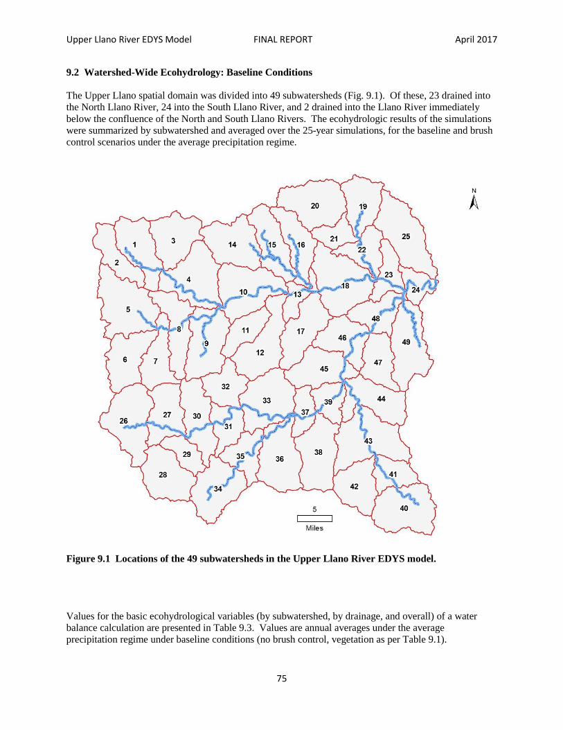
Upper Llano River EDYS Model FINAL REPORT April 2017
75
9.2 Watershed-Wide Ecohydrology: Baseline Conditions The Upper Llano spatial domain was divided into 49 subwatersheds (Fig. 9.1). Of these, 23 drained into the North Llano River, 24 into the South Llano River, and 2 drained into the Llano River immediately below the confluence of the North and South Llano Rivers. The ecohydrologic results of the simulations were summarized by subwatershed and averaged over the 25-year simulations, for the baseline and brush control scenarios under the average precipitation regime.
Figure 9.1 Locations of the 49 subwatersheds in the Upper Llano River EDYS model.
Values for the basic ecohydrological variables (by subwatershed, by drainage, and overall) of a water balance calculation are presented in Table 9.3. Values are annual averages under the average precipitation regime under baseline conditions (no brush control, vegetation as per Table 9.1).

Upper Llano River EDYS Model FINAL REPORT April 2017
76
Table 9.3 Average annual water balance components by watershed simulated for 25-year baseline scenario, expressed as watershed totals, using the Upper Llano EDYS model. Watershed Area Precipitation Watershed Totals (acre-feet) (acres) (acre-feet) Runoff ET GW-Use Recharge Direct Yield Storage + Seepage North Llano 01 26,792 51,651 3,480 44,730 22 0 3,458 3,463 02 18,057 34,947 210 30,852 0 13 223 3,872 03 26,231 50,758 645 42,382 0 18 663 7,713 04 35,054 67,830 6,008 54,883 117 0 5,891 7,056 05 38,991 75,448 940 65,956 65 85 960 8,532 06 26,167 50,742 1,072 44,809 0 77 1,149 4,784 07 20,872 40,438 1,026 35,688 0 0 1,026 3,724 08 25,004 48,382 2,542 42,796 21 0 2,521 3,065 09 32,671 63,218 404 53,113 136 0 268 9,837 10 34,955 69,853 1,199 59,129 3,934 173 - 2,562 13,286 11 15,603 31,167 215 25,535 0 0 215 5,417 12 30,991 61,931 2,394 53,560 181 89 2,302 6,069 13 10,530 21,042 7,123 23,833 5,162 129 2,090 - 4,881 14 29,712 59,374 518 46,444 25 0 493 12,437 15 25,216 50,391 154 43,033 1,577 18 - 1,405 8,763 16 22,872 45,707 168 40,768 3,356 85 - 3,103 8,042 17 27,400 54,754 3,632 47,445 297 20 3,355 3,954 18 38,576 77,122 1,637 63,678 804 876 1,709 11,735 19 22,598 45,178 3,987 36,248 603 30 3,414 5,516 20 32,646 65,265 1,195 52,555 82 0 1,113 11,597 21 11,577 23,144 8,768 18,425 58 100 8,810 - 4,091 22 17,043 34,072 221 28,460 369 131 - 17 5,629 23 15,067 30,122 507 25,863 666 647 488 3,771 Total 584,625 1,152,536 48,045 980,185 17,475 2,491 33,061 139,290
South Llano 26 35,294 72,030 196 65,027 0 372 568 6,435 27 24,006 48,933 7,248 44,010 0 72 7,320 - 2,397 28 28,207 57,591 303 51,712 0 106 409 5,470 29 12,377 25,271 4,383 22,588 31 65 4,417 - 1,734 30 26,669 54,227 4,062 48,735 22 60 4,100 1,392 31 15,996 32,659 80 29,258 40 72 112 3,289 32 18,456 36,974 478 32,327 15 40 503 4,144 33 33,315 67,715 491 61,299 361 101 231 6,185 34 30,460 62,901 221 56,045 0 136 357 6,499 35 17,814 36,786 1,253 32,702 0 66 1,319 2,765 36 32,829 67,793 645 60,349 0 146 791 6,653 37 11,698 24,147 116 21,524 127 104 93 2,530 38 32,080 66,247 1,865 59,401 0 192 2,057 4,789 39 13,605 28,004 2,035 24,646 45 30 2,020 1,338 40 33,723 68,346 417 60,193 0 149 566 7,587 41 15,168 30,741 3,305 26,847 13 77 3,369 525 42 23,416 47,456 350 42,303 0 139 489 4,664 43 39,629 80,315 3,833 71,395 0 176 4,009 4,911 44 27,294 55,202 436 47,943 23 119 532 6,727 45 26,212 52,446 1,826 42,109 219 158 1,765 8,572 46 23,218 46,436 1,306 37,532 1,568 297 35 8,869 47 19,666 39,349 1,799 31,250 33 26 1,792 6,307 48 19,170 38,340 599 35,543 5,210 889 - 3,722 6,519 49 32,883 65,794 906 53,568 603 179 482 11,744 Total 593,185 1,205,703 38,153 1,058,306 8,310 3,771 33,614 113,783
Llano 24 11,214 22,418 253 20,380 1,010 1,122 365 1,673 25 35,563 71,097 1,041 59,090 534 197 704 11,303 Total 46,777 93,515 1,294 79,470 1,544 1,319 1,069 12,976
Overall 1,224,587 2,451,754 87,492 2,117,961 27,329 7,581 67,744 266,049

Upper Llano River EDYS Model FINAL REPORT April 2017
77
Annual precipitation averaged 24.03 inches, averaged over the entire watershed. Annual precipitation was slightly lower in the North Llano River drainage (23.66 inches) and higher in the South Llano River drainage (24.39 inches). The South Llano River drainage is slightly (1.5%) larger than the North Llano River drainage. Runoff is direct surface runoff that would be measured at the respective point of exit (e.g., lowest point of the subwatershed). The annual average runoff in this scenario averaged 87,492 acre-feet, or 3.6% of annual precipitation. This compares favorably with measured values from three studies in the Edwards Plateau: 2.9% and 3.5% on two sites at the Sonora Experiment Station (Thurow et al. 1988), 3.9% on a 13% slope area in the northern Edwards Plateau (Wright et al. 1976), and 4.2% on a site in the eastern Edwards Plateau (Banta and Slattery 2011). Runoff varied substantially among subwatersheds in the simulations, ranging from 154 acre-feet to 8,768 acre-feet per year. This variability was primarily the result of differences in slope, soils, and vegetation among the subwatersheds, rather than size of the subwatershed. Averaged over the entire basin, mean annual runoff was equal to 0.86 inches per acre. Evapotranspiration (ET) averaged 2,117,961 acre-feet per year (Table 9.3), or 86.4% of annual precipitation. This is similar to values reported for an oak-grassland at the Sonora Experiment Station (95%, Thurow et al. 1987) and an Ashe juniper woodland in the eastern Edwards Plateau (83%, Banta and Slattery 2011). The simulated value was equal to 20.46 inches per year, averaged over the entire basin. EDYS simulates vegetation water use by tracking water removal at each soil layer, at each time step, by each plant species. Included in that accounting is water taken from saturated zones, i.e., groundwater. Groundwater-use (GW-Use, Table 9.3) is the sum of that water usage over the respective subwatershed. Under baseline conditions (Table 9.3), the vegetation utilized an average of 27,329 acre-feet of groundwater per year. This amount was equal to 0.27 inch per acre annually, or 1.3% of total ET. Groundwater usage varied among the subwatersheds, with highest use in subwatersheds 13 and 48 which both had large amounts of their respective areas in floodplains (Fig. 3.1). Subwatersheds with no groundwater use were generally located in upper elevation areas. Recharge is the amount of water entering into groundwater. It is the amount that moves through the soil profile, either at the point of origin or by surface movement (runoff) that then enters the profile. Recharge in the baseline simulation (Table 9.3) averaged 7,581 acre-feet per year over the entire basin. This was equal to 0.07 inch per acre per year, or 0.3% of annual precipitation. Direct yield is the minimum amount of average annual water yield from the respective subwatershed. It was calculated as: direct yield = runoff + recharge – groundwater use. This calculation is a conservative calculation (i.e., actual direct yield is probably greater than this amount) because some of what EDYS calculates as soil storage probably enters either the surface water or groundwater pools by movement through cracks, channels, and fissures in the underlying rocks. Direct yield under baseline conditions averaged 67,744 acre-feet per year for the basin (Table 9.3), or 0.66 inch per acre per year. This is equal to 2.8% of annual precipitation. Storage is the average annual amount of water entering the soil system (infiltrated water) and not exported by ET or recharge. It is the net balance in water retained in the soil, by soil layer. It is calculated by: Storage = precipitation + groundwater use – ET – runoff – recharge.

Upper Llano River EDYS Model FINAL REPORT April 2017
78
Some of this water likely exits the soil system as seepage and spring flow and should therefore be added to direct yield. However, without knowing the subsurface geologic structures, we cannot directly model that lateral flow. Under the baseline scenario (Table 9.3), 266,049 acre-feet of water was added to the soil profile each year. This equals 2.61 inches per year, or 10.9% of annual precipitation. Seepage. The potential available water holding capacity of a typical soil in the models is about 15% by volume in the upper 1.25 m, 5% in the next 8.5 m, and 1% in the lowest layers down to 28 m (Table 5.4). This would equal a total potential available water holding capacity of 80 cm, or 31.5 inches. Averaged over all soil types by area covered, the mean available water holding capacity for the EDYS soil profiles across the entire watershed is 28.50 inches. An average annual storage value of 2.61 inches (previous paragraph) would equal a 25-year total soil storage of 65.75 inches, or over twice the available waterholding capacity of the profiles. In EDYS, this water in excess of available water holding capacity is stored as saturated zones within the soil profile (i.e., perched water tables and pooled water in karst structures). In fact, some would likely be held as perched water tables or pockets of free water in karst features and some would likely move laterally and become seepage or spring flow. If all of the surplus storage water (36.5 inches averaged across the watershed) became seepage or spring flow, this would equal 56% of the calculated annual soil storage value. This would increase direct yield by 148,987 acre-feet per year. More likely, only part of this surplus would become direct yield, the remaining portion being retained in the soil profile. Median flow of the Llano River at Junction is 109 cfs (Broad et al. 2016), or 78,916 acre-feet per year. The EDYS baseline direct yield is 67,744 acre-feet per year. The difference between these two values, 11,172 acre-feet per year, is one estimate of the amount of EDYS storage that moves into the surface water supply as lateral flow to seeps and springs. This amount (11,172 acre-feet) is 7.5% of the storage water in excess of maximum available water holding capacity. This seems reasonable. Based on the total storage value (266,049 acre-feet, Table 9.3), this estimated seep and spring flow from storage would equal 4.2% of total storage. In summary, under baseline conditions averaged over the 25-year simulation total annual water supply (precipitation plus groundwater usage) was 2,479,083 acre-feet (Fig. 9.2). Of this, ET accounted for 85.4%, runoff 3.5%, groundwater recharge 0.3%, seep and spring flow 0.5%, and storage within the soil and subsoil system 10.3%.

Upper Llano River EDYS Model FINAL REPORT April 2017
79
Figure 9.2 Annual (25-year mean) water-balance (acre-feet and % of supply) for the Upper Llano River watershed under baseline (average precipitation regime, no brush control).

Upper Llano River EDYS Model FINAL REPORT April 2017
80
9.3 Watershed-Wide Ecohydrology: Brush Control Scenario Under the brush control scenario, there was a slight increase (0.5%) in ET and a small (1.0%) decrease in groundwater use by vegetation (Table 9.4) compared to baseline conditions. The increase in ET was the result of two factors. First, there was an increase in production by herbaceous species following the reduction in density of woody plants. Second, there was regrowth of the tree and shrub species over time. The regrowth was more productive on an annual basis than the previous old-growth trees. In practice, re-treatment of brush controlled areas is necessary in order to maintain the benefits of brush removal. Without retreatment, the woody species will regain dominance because of secondary succession. The decrease in groundwater use was the result of an initial reduction in deeper-rooted woody species. This benefit decreased over time as the woody species re-established. Runoff decreased by 9.7% in response to brush control. This was the result of increased herbaceous production, which slowed runoff and allowed more water to enter into the soil. Brush control increased recharge by 11.0% because of increased infiltration (i.e., reduced runoff) and less use of deep soil moisture by woody vegetation. Direct yield, when measured only by runoff and recharge, decreased by 10.8% (7,342 acre-feet per year) because the decrease in runoff exceeded the increase in recharge.

Upper Llano River EDYS Model FINAL REPORT April 2017
81
Table 9.4 Average annual water balance components by watershed simulated for brush control (50-100% cover) scenario, expressed as watershed totals, using the Upper Llano EDYS model. Watershed Area Precipitation Watershed Totals (acre-feet) (acres) (acre-feet) Runoff ET GW-Use Recharge Direct Yield Storage + Seepage North Llano 01 26,792 51,651 2,996 44,797 0 0 2,996 3,858 02 18,057 34,947 317 30,867 0 13 330 3,750 03 26,231 50,758 900 42,447 22 18 896 7,415 04 35,054 67,830 4,973 55,029 117 0 4,856 7,945 05 38,991 75,448 954 66,086 98 85 941 8,421 06 26,167 50,742 1,061 44,852 0 77 1,138 4,752 07 20,872 40,438 1,023 35,740 17 0 1,006 3,692 08 25,004 48,382 2,763 42,858 63 0 2,700 2,824 09 32,671 63,218 483 53,276 245 0 238 9,704 10 34,955 69,853 1,199 60,149 4,721 151 - 3,371 13,075 11 15,603 31,167 286 25,691 13 0 273 5,203 12 30,991 61,931 2,071 54,309 310 91 1,852 5,770 13 10,530 21,042 5,497 26,353 7,541 132 - 1,912 - 3,399 14 29,712 59,374 1,416 46,642 0 0 1,416 11,316 15 25,216 50,391 239 43,643 1,745 18 - 1,488 8,236 16 22,872 45,707 231 42,427 4,176 71 - 3,874 7,154 17 27,400 54,754 2,940 48,313 594 20 2,366 4,075 18 38,576 77,122 1,717 64,064 804 882 1,795 11,263 19 22,598 45,178 3,265 37,378 622 31 2,674 5,126 20 32,646 65,265 1,183 53,780 54 0 1,129 10,356 21 11,577 23,144 7,557 18,705 48 101 7,610 - 3,171 22 17,043 34,072 274 28,659 355 131 50 5,363 23 15,067 30,122 484 25,939 603 660 541 3,642 Total 584,625 1,152,536 43,829 992,004 22,148 2,481 24,162 136,370
South Llano 26 35,294 72,030 279 64,998 0 372 651 6,381 27 24,006 48,933 5,906 43,950 0 90 5,996 - 1,013 28 28,207 57,591 381 51,665 0 148 529 5,397 29 12,377 25,271 4,298 22,588 31 65 4,332 - 1,649 30 26,669 54,227 2,933 48,713 22 80 2,991 2,523 31 15,996 32,659 85 29,218 13 84 156 3,285 32 18,456 36,974 488 32,327 15 54 527 4,120 33 33,315 67,715 528 61,354 389 126 265 6,096 34 30,460 62,901 233 55,994 0 181 414 6,493 35 17,814 36,786 1,219 32,687 0 92 1,311 2,788 36 32,829 67,793 700 60,239 0 243 943 6,611 37 11,698 24,147 133 21,368 20 155 268 2,511 38 32,080 66,247 1,827 59,294 0 287 2,114 4,839 39 13,605 28,004 1,862 24,646 79 80 1,863 1,495 40 33,723 68,346 459 60,165 0 223 682 7,499 41 15,168 30,741 2,136 26,796 0 99 2,235 1,710 42 23,416 47,456 655 42,244 0 156 811 4,401 43 39,629 80,315 2,708 71,263 0 293 3,001 6,051 44 27,294 55,202 544 47,921 23 178 699 6,582 45 26,212 52,446 1,762 42,350 109 159 1,812 8,284 46 23,218 46,436 1,417 36,874 523 307 1,201 8,361 47 19,666 39,349 1,680 31,791 33 40 1,687 5,871 48 19,170 38,340 593 32,538 1,918 827 - 498 6,300 49 32,883 65,794 926 54,116 219 203 910 10,768 Total 593,185 1,205,703 33,752 1,055,099 3,394 4,542 34,900 115,704
Llano 24 11,214 22,418 250 20,221 776 1,138 612 1,585 25 35,563 71,097 1,216 60,631 741 253 728 9,738 Total 46,777 93,515 1,466 80,852 1,517 1,391 1,340 11,323
Overall 1,224,587 2,451,754 79,047 2,127,955 27,059 8,414 60,402 263,397

Upper Llano River EDYS Model FINAL REPORT April 2017
82
9.4 Selection of Subwatershed for Treatment The effects of brush control on potential enhanced water yield vary spatially across watersheds (Fish and Rainwater 2007, McLendon et al. 2012a, McLendon 2013). Because of spatial variation, brush control should not be expected to result in substantial enhancement of water yield when applied indiscriminately across a watershed. Instead, specific areas with high potential for enhanced water yield should be identified and brush control applied to these identified areas. Potential for enhanced water yield from brush control varied substantially among the 49 Upper Llano River subwatersheds (Fig. 9.3). Increases in direct yield from the brush control simulation occurred in half (25) of the Upper Llano River subwatersheds. The average annual enhanced yield from these 25 subwatersheds totaled 7,938 acre-feet per year (Table 9.5). This would equal a 12% increase in direct yield over baseline conditions (Table 9.3).
Figure 9.3 Potential for increased water yield (acre-feet per year) from brush control in the 49 subwatersheds of the Upper Llano River watershed. Values are 25-year means under the average precipitation regime.

Upper Llano River EDYS Model FINAL REPORT April 2017
83
Table 9.5 Direct water yield and net storage under baseline (Table 9.3) and brush control (Table 9.4) scenarios, 25-year annual means at moderate precipitation, Upper Llano EDYS model. Watershed Direct Yield (ac-ft) Enhancement (ac-ft) Storage + Seepage (ac-ft) Enhancement (ac-ft) Baseline Brush Control (BC – Baseline) Baseline Brush Control (BC – Baseline) North Llano 01 3,458 2,996 - 462 3,463 3,858 395 02 223 330 107 3,872 3,750 - 122 03 663 896 233 7,713 7,415 - 298 04 5,891 4,856 - 1,035 7,056 7,945 889 05 960 941 - 19 8,532 8,421 - 111 06 1,149 1,138 - 11 4,784 4,752 - 32 07 1,026 1,006 - 20 3,724 3,692 - 32 08 2,521 2,700 179 3,065 2,824 - 241 09 268 238 - 30 9,837 9,704 - 133 10 - 2,562 - 3,371 - 809 13,286 13,075 - 211 11 215 273 58 5,417 5,203 - 214 12 2,302 1,852 - 450 6,069 5,770 - 299 13 2,090 - 1,912 - 4,002 - 4,881 - 3,399 1,482 14 493 1,416 923 12,437 11,316 - 1,121 15 - 1,405 - 1,488 - 83 8,763 8,236 - 527 16 - 3,103 - 3,874 - 771 8,042 7,154 - 888 17 3,355 2,366 - 989 3,954 4,075 121 18 1,709 1,795 86 11,735 11,263 - 472 19 3,414 2,674 - 740 5,516 5,126 - 390 20 1,113 1,129 16 11,597 10,356 - 1,241 21 8,810 7,610 - 1,200 - 4,091 - 3,171 920 22 - 17 50 67 5,629 5,363 - 266 23 488 541 53 3,771 3,642 - 129 Total 33,061 24,162 - 8,899 139,290 136,370 - 2,920
South Llano 26 568 651 83 6,435 6,381 - 54 27 7,320 5,996 - 1,324 - 2,397 - 1,013 1,384 28 409 529 120 5,470 5,397 - 73 29 4,417 4,332 - 85 - 1,734 - 1,649 85 30 4,100 2,991 - 1,109 1,392 2,523 1,131 31 112 156 44 3,289 3,285 - 4 32 503 527 24 4,144 4,120 - 24 33 231 265 34 6,185 6,096 - 89 34 357 414 57 6,499 6,493 - 6 35 1,319 1,311 - 8 2,765 2,788 23 36 791 943 152 6,653 6,611 - 42 37 93 268 175 2,530 2,511 - 19 38 2,057 2,114 57 4,789 4,839 50 39 2,020 1,863 - 157 1,338 1,495 157 40 566 682 116 7,587 7,499 - 88 41 3,369 2,235 - 1,134 525 1,710 1,185 42 489 811 322 4,664 4,401 - 263 43 4,009 3,001 - 1,008 4,911 6,051 1,140 44 532 699 167 6,727 6,582 - 145 45 1,765 1,812 47 8,572 8,284 - 288 46 35 1,201 1,166 8,869 8,361 - 508 47 1,792 1,687 - 105 6,307 5,871 - 436 48 - 3,722 - 498 3,224 6,519 6,300 - 219 49 482 910 428 11,744 10,768 - 976 Total 33,614 34,900 1,286 113,783 115,704 1,921
Llano 24 365 612 247 1,673 1,585 - 88 25 704 728 24 11,303 9,738 - 1,565 Total 1,069 1,340 271 12,976 11,323 - 1,653
Overall 67,744 60,402 - 7,342 266,049 263,397 - 2,652

Upper Llano River EDYS Model FINAL REPORT April 2017
84
The simulated brush treatment was not applied to the entire area within each of the 25 subwatersheds with potential water enhancement. Only those areas within the subwatershed with 50% of more woody plant cover and less than 12% slope were included in the brush treatment. The total area in these 25 subwatersheds with potential for water enhancement was 642,190 acres, or 52.4% of the total area of the watershed (1,224,587 acres). Of the 642,190 acres in the 25 subwatersheds with potential for water enhancement, only 177,326 acres (27.6%) were treated (Table 9.6). Therefore, the potential increase in water yield (7,938 acre-feet per year = 2,586,605,000 gallons) would be the result of the treatment of 177,326 acres. This amount can be expressed as an annual increased yield of 0.045 acre-feet (14,663 gallons) of increased yield per treated acre, or a 25-year total return of 1.13 acre-feet (368,212 gallons) per treated acre. Two-thirds (5,313 acre-feet = 1,731,246,363 gallons) of the total potential enhanced yield resulted from treatment of 25,475 acres in three subwatersheds (14, 46, and 48; Table 9.6). The potential enhanced yield from treatment of these three subwatersheds was 0.208 acre-feet (67,777 gallons) per treated acre per year, or 5.20 acre-feet (1,694,425 gallons) over the 25 years.

Upper Llano River EDYS Model FINAL REPORT April 2017
85
Table 9.6 Potential annual enhanced water yield from the brush control (50-100% cover) scenario, 25-year mean at moderate precipitation regime, Upper Llano EDYS model. Watershed Area (acres) Treated/ Potential Enhanced Annual Yield Storage + Seepage Total Treated Total Overall Per Treated Acre Overall Treated Acre (103 gallons) (ac-ft) (gallons) (inches) (103 gallons) (gallons) North Llano 01 26,792 5,520 0.206 - 150,543 - 462 - 27,272 - 1.004 1,257,133 227,742 02 18,057 3,235 0.179 34,866 107 10,778 0.397 1,221,941 377,725 03 26,231 10,156 0.387 75,923 233 7,476 0.275 2,416,185 237,907 04 35,054 12,129 0.346 - 337,256 - 1,035 - 27,806 - 1.024 2,588,886 213,446 05 38,991 12,869 0.330 - 6,191 - 19 - 481 - 0.018 2,743,991 213,225 06 26,167 9,576 0.367 - 3,584 - 11 - 374 - 0.014 1,548,444 161,700 07 20,872 5,959 0.286 - 6,517 - 20 - 1,094 - 0.040 1,203,042 201,887 08 25,004 7,559 0.302 58,327 179 7,716 0.284 920,203 121,736 09 32,671 8,662 0.259 - 9,776 - 30 - 1,129 - 0.042 3,162,058 365,049 10 34,955 11,797 0.338 - 263,613 - 809 - 22,346 - 0.823 4,260,502 361,151 11 15,603 7,213 0.462 18,899 58 2,620 0.096 1,695,403 235,048 12 30,991 12,794 0.413 - 146,633 - 450 - 11,461 - 0.422 1,880,160 146,956 13 10,530 3,683 0.349 -1,304,056 - 4,002 - 354,074 -13.039 - 1,107,568 – 300,724 14 29,712 9,943 0.335 300,760 923 30,248 1.114 3,687,330 370,847 15 25,216 6,662 0.264 - 27,046 - 83 - 4,060 - 0.150 2,683,709 402,838 16 22,872 11,227 0.491 - 251,231 - 771 - 22,377 - 0.824 2,331,138 207,637 17 27,400 9,037 0.330 - 322,267 - 989 - 35,661 - 1.313 1,327,843 146,934 18 38,576 11,839 0.307 28,023 86 2,367 0.087 3,670,060 309,997 19 22,598 13,095 0.579 - 241,130 - 740 - 18,414 - 0.678 1,670,312 127,553 20 32,646 15,522 0.475 5,214 16 336 0.012 3,374,513 217,402 21 11,577 6,409 0.554 - 391,021 - 1,200 - 61,011 - 2.247 - 1,033,274 – 161,222 22 17,043 5,247 0.308 21,832 67 4,161 0.153 1,747,539 333,055 23 15,067 4,251 0.282 17,270 53 4,063 0.150 1,186,749 279,169 Total 584,625 204,384 0.350 -2,899,748 - 8,899 44,436,301 Mean - 14,188 - 0.522 217,416
South Llano 26 35,294 6,184 0.175 27,046 83 4,373 0.161 2,079,255 336,231 27 24,006 2,308 0.096 - 431,427 - 1,324 – 186,927 - 6.884 - 330,087 – 143,019 28 28,207 6,086 0.216 39,102 120 6,425 0.236 1,758,618 288,961 29 12,377 1,185 0.096 - 27,697 - 85 - 23,373 - 0.861 - 537,328 – 453,442 30 26,669 2,171 0.081 - 361,369 - 1,109 - 166,453 - 6.130 822,122 378,684 31 15,996 2,454 0.153 14,337 44 5,842 0.215 1,070,421 436,194 32 18,456 2,743 0.148 7,820 24 2,851 0.105 1,342,506 489,430 33 33,315 4,809 0.144 11,079 34 2,304 0.085 1,986,388 413,056 34 30,460 5,009 0.164 18,574 57 3,708 0.136 2,115,751 422,390 35 17,814 1,287 0.072 - 2,607 - 8 - 2,025 - 0.068 908,473 705,884 36 32,829 6,445 0.196 49,529 152 7,685 0.283 2,154,201 334,244 37 11,698 3,658 0.313 57,024 175 15,589 0.574 818,212 223,677 38 32,080 6,927 0.216 18,574 57 2,681 0.099 1,576,793 227,630 39 13,605 3,265 0.240 - 51,159 - 157 - 15,669 - 0.577 487,147 149,203 40 33,723 10,093 0.299 37,799 116 3,745 0.138 2,443,557 242,104 41 15,168 2,851 0.188 - 369,515 - 1,134 - 129,609 - 4.773 557,205 195,442 42 23,416 3,926 0.168 104,924 322 26,725 0.984 1,434,070 365,275 43 39,629 16,236 0.410 - 328,458 - 1,008 - 20,230 - 0.745 1,971,724 121,442 44 27,294 8,113 0.297 54,417 167 6,707 0.247 2,144,751 264,360 45 26,212 5,272 0.201 15,315 47 2,905 0.107 2,699,350 512,016 46 23,218 7,495 0.323 379,942 1,166 50,693 1.867 2,724,440 363,501 47 19,666 7,633 0.383 - 34,214 - 105 - 4,482 - 0.165 1,913,071 250,632 48 19,170 8,037 0.419 1,050,544 3,224 130,713 4.814 2,052,861 255,426 49 32,883 15,110 0.460 139,464 428 9,230 0.340 3,508,764 232,215 Total 593,185 139,297 0.235 419,044 1,286 37,702,264 Mean 3,008 0.111 270,661
Llano 24 11,214 3,945 0.352 80,485 247 20,402 0.751 516,474 130,919 25 35,563 20,747 0.583 7,820 24 377 0.014 3,173,137 152,944 Total 46,777 24,692 0.528 88,305 271 3,689,611 Mean 3,576 0.132 149,425
Overall 1,224,587 368,373 0.301 - 2,392,399 - 7,342 85,828,176 Mean - 6,495 - 0.239 232,993

Upper Llano River EDYS Model FINAL REPORT April 2017
86
Based on potential enhanced per-acre water yields from the simulations, five subwatersheds have the highest potential and 16 subwatersheds have a moderate potential for enhanced water yield from brush control (Table 9.7 and Fig. 9.4). Table 9.7. Ranking of watersheds in order of potential annual enhanced water yield (gallons per treated acre and inches per treated acre) from the application of brush control to areas supporting 50-100% woody plant cover scenario, 25-year mean values at moderate precipitation regime, Upper Llano EDYS model. Watershed Yield (gallons) Yield (inches) Watershed Yield (gallons) Yield (inches) Higher Potential Yield Moderate Potential Yield 48 South Llano 130,713 4.81 37 South Llano 15,589 0.57 46 South Llano 50,693 1.87 02 North Llano 10,778 0.40 14 North Llano 30,248 1.11 49 South Llano 9,230 0.34 42 South Llano 26,725 0.98 08 North Llano 7,716 0.28 24 Llano 20,402 0.75 36 South Llano 7,685 0.28 03 North Llano 7,476 0.28 44 South Llano 6,707 0.25 28 South Llano 6,425 0.24 31 South Llano 5,842 0.22 26 South Llano 4,373 0.16 22 North Llano 4,161 0.15 23 North Llano 4,063 0.15 40 South Llano 3,745 0.14 34 South Llano 3,708 0.14 45 South Llano 2,905 0.11 32 South Llano 2,851 0.11
Lower Potential Yield Negative Potential Yield 38 South Llano 2,681 0.10 06 North Llano - 374 - 0.01 11 North Llano 2,620 0.10 05 North Llano - 481 - 0.02 18 North Llano 2,367 0.09 07 North Llano - 1,094 - 0.04 33 South Llano 2,304 0.09 09 North Llano - 1,129 - 0.04 25 Llano 377 0.01 35 South Llano - 2,025 - 0.07 20 North Llano 336 0.01 15 North Llano - 4,060 - 0.15 47 South Llano - 4,482 - 0.17 12 North Llano - 11,461 - 0.42 39 South Llano - 15,669 - 0.58 19 North Llano - 18,414 - 0.68 43 South Llano - 20,230 - 0.75 10 North Llano - 22,346 - 0.82 16 North Llano - 22,377 - 0.82 29 South Llano - 23,373 - 0.86 01 North Llano - 27,272 - 1.00 04 North Llano - 27,806 - 1.02 17 North Llano - 35,661 - 1.31 21 North Llano - 61,011 - 2.25 41 South Llano -129,609 - 4.77 30 South Llano -166,453 - 6.13 27 South Llano -186,927 - 6.88 13 North Llano -354,074 -13.04

Upper Llano River EDYS Model FINAL REPORT April 2017
87
Figure 9.4 Location of subwatersheds ranked in order of potential for enhanced water yield (gallons per treated acre per year) from brush control on areas supporting 50-100% woody plant cover, under the average precipitation regime, Upper Llano River EDYS models.

Upper Llano River EDYS Model FINAL REPORT April 2017
88
10.0 LITERATURE CITED Adiku, S.G.K., C.W. Rose, R.D. Braddock, and H. Ozier-Lafontaine. 2000. On the simulation of root water extraction: examination of a minimum energy hypothesis. Soil Science 165:226-236. Albertson, F.W. 1937. Ecology of mixed prairie in west central Kansas. Ecological Monographs 7:481-547. Amerikanuak, Inc. 2006. Proposal for the TVX Mineral Hill Mine consolidated closure plan modifications near Gardiner, Montana. Report submitted to the Montana Department of Environmental Quality. Submitted by TVX Mineral Hill, Inc. Toronto, Ontario. 139 p. Anderson, Kling L., Ed F. Smith, and Clenton E. Owensby. 1970. Burning bluestem range. Journal of Range Management 23:81-92. Andersson, F. 1970. Ecological studies in a Scanian woodland and meadow area, southern Sweden. II. Plant biomass, primary production, and turnover of organic matter. Bot. Notiser 123:8-51. Archer, Steve, Charles Scifres, C.R. Bassham, and Robert Maggio. 1988. Autogenic succession in a subtropical savanna: conversion of grassland to thorn woodland. Ecological Monographs 58:111-127. Arnold, J.F. and H.G. Reynolds. 1943. Droppings of Arizona antelope jackrabbits and the pellet census. Journal of Wildlife Management 7:322-327. Ash, Andrew and Lynn Walker. 1999. Environmental management of military lands. LWRRDC Project CTC19. Constructing decision support tools to evaluate management alternatives. Final Report. CSIRO Tropical Agriculture. Aitkenvale, Queensland, Australia. 37 p. Atkins, M.D. and J.E. Smith, Jr. 1967. Grass seed production and harvest in the Great Plains. USDA Farmer’s Bulletin 2226. Washington, DC. 30 p. Ayensu, Edward S. (ed.). 1980. Firewood Crops. Shrub and Tree Species for Energy Production. National Academy of Sciences. Washington DC. 237 p. Bailey, Robert G. 1995. Description of the Ecoregions of the United States. USDA Forest Service Misc. Publication 1391. 108 p. Banta, J. Ryan and Richard N. Slattery. 2011. Effects of brush management on the hydrologic budget and water quality in and adjacent to Honey Creek State Natural Area, Comal County, Texas, 2001-10. USGS Scientific Investigations Report 2011-5226. 35 p. Barth, R.C. and J.O. Klemmedson.1982. Amount and distribution of dry matter, nitrogen, and organic carbon in soil-plant systems of mesquite and palo verde. Journal of Range Management 35:412-418. Beaty, E.R., K.H. Tan, R.A. McCreery, and J.B. Jones. 1973. Root-herbage production and nutrient uptake and retention by bermudagrass and bahiagrass. Journal of Range Management 28:385-389. Bjorck, Svante, Bernd Kromer, Sigfus Johnen, Ole Bennike, Dan Hammarlund, Geoffrey Lemdahl, Goran Possneret, Tine Lander Rasmussen, Barbara Wohlfarth, Claus Uffe Hammer, and Marco Spurk. 1996. Synchronized terrestrial-atmospheric deglacial records around the North Atlantic. Science 274:1155-1160

Upper Llano River EDYS Model FINAL REPORT April 2017
89
Blum, Ervin L. 1982. Soil survey of Kimble County, Texas. USDA Soil Conservation Service. Washington DC. 99 p + maps. Box, Thadis W. 1961. Relationships between plants and soils of four range plant communities in South Texas. Ecology 42:794-810. Box, Thadis W. and A. Dean Chamrad. 1966. Plant Communities of the Welder Wildlife Refuge. Contribution No. 5, Series B. Welder Wildlife Foundation. Sinton, Texas. 28 p. Boyd, I.L. 1943. Germination tests on four species of sumac. Transactions of the Kansas Academy of Science 46:85-86. Bremer, Dale J., Lisa M. Auren, Jay M. Ham, and Clenton E. Owensby. 2001. Evapotranspiration in a prairie ecosystem: effects of grazing by cattle. Agronomy Journal 93:338-348. Brinkman, K.A. 1974. Rhus L., Sumac. In: C.S. Schopmeyer (ed.) Seeds of Woody Plants in the United States. USDA Agriculture Handbook 450. Washington DC. pp 715-719. Broad, Tyson, Emily Seldomridge, Tom Arsuffi, and Kevin Wagner. 2016. Upper Llano River Watershed Protection Plan. Developed by the Upper Llano Watershed Coordination Committee. Texas Tech University, Lubbock and Texas Water Resources Institure, College Station. 178 p. Brock, J.H., W.H. Blackburn, and R.H. Haas. 1982. Infiltration and sediment production on a deep hardland range site in north central Texas. Journal of Range Management 35:195-198. Bryant, F.C., M.M. Kothmann, and L.B. Merrill. 1979. Diets of sheep, Angora goats, Spanish goats, and white-tailed deer under excellent range conditions. Journal of Range Management 32:412-417. Buyanovsky, G.A., C.L. Kucera, and G.H. Wagner. 1987. Comparative analyses of carbon dynamics in native and cultivated ecosystems. Ecology 68:2023-2031. Caldwell, M.M. and L.B. Camp. 1974. Belowground productivity of two cool desert communities. Oecologia 17:123-139. Caldwell, Martyn M., Richard S. White, Russell T. Moore, and L.B. Camp. 1977. Carbon balance, productivity, and water use of cold-winter desert shrub communities dominated by C3 and C4 species. Oecologia 29:275-300. Carlson, D.H., T.L. Thurow, R.W. Knight, and R.K. Heitschmidt. 1990. Effect of honey mesquite on the water balance of Texas Rolling Plains rangeland. Journal of Range Management 43:491-496. Cayan, Daniel R., Kelly T. Redmond, and Laurence G. Riddle. 1999. ENSO and hydrologic extremes in the western United States. Journal of Climate 12:2881-2893. Chamrad, A. Dean, Billie E. Dahl, John G. Kie, and D. Lynn Drawe. 1979. Deer food habits in South Texas – Status, needs, and role in resource management. In: D. Lynn Drawe (ed.) Proceedings of the First Welder Wildlife Foundation Symposium. Welder Wildlife Foundation Contribution B-7. Sinton, Texas. pp 132-142. Childress, W. Michael and Terry McLendon. 1999. Simulation of multi-scale environmental impacts using the EDYS model. Hydrological Science and Technology 15:257-269.

Upper Llano River EDYS Model FINAL REPORT April 2017
90
Childress, W. Michael, Terry McLendon, and David L. Price. 1999a. A decision support system for allocation of training activities on US Army installations. In: Jeffrey M. Klopatek and Robert H. Gardner (eds.). Landscape Ecological Analysis: Issues, Challenges, and Ideas. Ecological Studies Series. Springer-Verlag. New York. pp 80-108. Childress, W. Michael, David L. Price, Cade L. Coldren, and Terry McLendon. 1999b. A functional description of the Ecological Dynamics Simulation (EDYS) model, with applications for Army and other Federal land managers. US Army Corps of Engineers CERL Technical Report 99/55. 68 p. Childress, W. Michael, Cade L. Coldren, and Terry McLendon. 2002. Applying a complex, general ecosystem model (EDYS) in large-scale land management. Ecological Modelling 153:97-108. Chiles, Gary W. and Terry McLendon. 2004. Sustainable range management system. Federal Facilities Environmental Journal 15:41-49. Chimner, Rodney A. and David J. Cooper. 2004. Using stable oxygen isotopes to quantify the water source used for transpiration by native shrubs in the San Luis Valley, Colorado, USA. Plant and Soil 260:225-236. Chumbley, C.A., R.G. Baker, and E.A. Bettis III. 1990. Midwestern Holocene paleoenvironments revealed by floodplain deposits in northwestern Iowa. Science 249:272-274. Coffee, Daniel R. 1967. Soil Survey of Menard County, Texas. USDA Soil Conservation Service. Washington DC. 51 p + maps. Coldren, Cade L., Terry McLendon, and W. Michael Childress. 2011a. Ecological DYnamics Simulation Model (EDYS) Users Guide. Version 5.1.0. KS2 Ecological Field Services LLC. Fort Collins, Colorado. 259 p. Coldren, Cade L., Terry McLendon, W. Michael Childress, David L. Price, and Mark R. Graves. 2011b. Ecological DYnamics Simulation Model – Light (EDYS-L). User’s Guide Version 4.6.4. US Army Corps of Engineers. Engineer Research and Development Center. ERDC/EL SR-11-1. 94 p. Comstock, Jonathan P. and James R. Ehleringer. 1992. Plant adaptation in the Great Basin and Colorado Plateau. Great Basin Naturalist 52:195-215. Cook, P.G. and A.P. O’Grady. 2006. Determining soil and ground water use of vegetation from heat pulse, water potential and stable isotope data. Oecologia 148:97-107. Correll, Donovan S. and Marshall C. Johnston. 1970. Manual of the Vascular Plants of Texas. Texas Research Foundation. Renner, Texas. 1881 p. Cottam, D.A. 1985. Frequency-dependent grazing by slugs and grasshoppers. Journal of Ecology 73:925-933. Coupland, R.T. and T.C. Bradshaw. 1953. The fescue grassland in Saskatchewan. Ecology 34:386-405. Cox, G.S. 1958. Root distribution in ponderosa pine stands growing on three soils. Proceedings of the Montana Academy of Sciences 19:135-141.

Upper Llano River EDYS Model FINAL REPORT April 2017
91
Coyne, P.I. and J.A. Bradford. 1986. Biomass partitioning in ‘Caucasian’ and ‘WW-Spar’ old-world bluestems. Journal of Range Management 39:303-310. Cramer, Viki A., Peter J. Thorburn, and Grant W. Fraser. 1999. Transpiration and groundwater uptake from farm forest plots of Casuarina glauca and Eucalyptus camaldulensis in saline areas of southeast Queensland, Australia. Agricultural Water Management 39:187-204. Dahl, Bill. 1994. Mesquite-buffalograss. In: Thomas N. Shiflet (ed.) Rangeland Cover Types of the United States. Society for Range Management. Denver, Colorado. pp 102-103. Dalrymple, R.L., D.D. Dwyer, and J.E. Webster. 1965. Cattle utilization and chemical content of winged elm browse. Journal of Range Management 18:126-128. Dawson, Todd E. 1993. Hydraulic lift and water use by plants: implications of water balance, performance, and plant-plant interactions. Oecologia 95:565-574. Dawson, Todd E. and James R. Ehleringer. 1991. Streamside trees that do not use stream water. Nature 350:335-337. Dawson, Todd E. and John S. Pate. 1996. Seasonal water uptake and movement in root systems of Australian phraeatophytic plants of dimorphic root morphology: A stable isotope investigation. Oecologia 107:13-20. Dittemore, William H., Jr. and Winfred C. Coburn. 1986. Soil Survey of Kerr County, Texas. USDA Soil Conservation Service. Washington DC. 123 p + maps. Donovan, L.A. and J.R. Ehleringer. 1994. Water stress and use of summer precipitation in a Great Basin shrub community. Functional Ecology 8:289-297. Dorale, Jeffrey A., Luis A. Gonzalez, Mark K. Reagan, David A. Pickett, Michael T. Murrell, and Richard G. Baker. 1992. A high-resolution record of Holocene climate change in speleothem calcite from Cold Water Cave, Northeast Iowa. Science 258:1626-1630. Drawe, D. Lynn and Thadis W. Box. 1968. Forage ratings for deer and cattle on the Welder Wildlife Refuge. Journal of Range Management 21:225-235. Drawe, D. Lynn and Thadis W. Box. 1969. High rates of nitrogen fertilization influence coastal prairie range. Journal of Range Management 22:32-36. Drawe, D. Lynn, A. Dean Chamrad, and Thadis W. Box. 1978. Plant Communities of the Welder Wildlife Refuge. Contribution No. 5, Series B, Revised. Welder Wildlife Foundation. Sinton, Texas. 38 p. Duell, L.F.W., Jr. 1990. Estimates of evapotranspiration in alkaline scrub and meadow communities of Owens Valley, California, using the Bowen-ratio, eddy-correlation, and Penman-combination methods. USGS Water Supply Paper 2370-E. 39 p. Durham, Albert J., Jr. and M.M. Kothmann. 1977. Forage availability and cattle diets on the Texas Coastal Prairie. Journal of Range Management 30:103-106. Duvall, Vinson L. and Norwin E. Linnartz. 1967. Influence of grazing and fire on vegetation and soil of longleaf pine-bluestem range. Journal of Range Management 20:241-247.

Upper Llano River EDYS Model FINAL REPORT April 2017
92
Duvigneaud, P., P. Kerstemont, and P. Ambroes. 1971. Productivite primaire des forets temperees d’essence feuilles caducifoliees en Europe occidentale. In: P. Duvigneaud (ed.) Productivity of Forest Ecosystems. UNESCO. Paris. Eddleman, L.E. 1977. Indigenous plants of southeastern Montana. I. Viability and suitability for reclamation in the Fort Union Basin. Montana Forestry and Conversation Experiment Station Special Publication 4. School of Forestry. University of Montana. Missoula. 122 p. Engle, David. 1994. Cross Timbers-Oklahoma. In: Thomas N. Shiflet (ed.) Rangeland Cover Types of the United States. Society for Range Management. Denver, Colorado. pp 90-91. Evans, T.L., R. Mata-Gonzalez, D.W. Martin, T. McLendon, and J.S. Noller. 2013. Growth, water productivity, and biomass allocation of Great Basin plants as affected by summer watering. Ecohydrology 6:713-721. Everitt, James H. and D. Lynn Drawe. 1974. Spring food habits of white-tailed deer in the South Texas plains. Journal of Range Management 27:15-20. Everitt, James H., C.L. Gonzalez, G. Scott, and B.E. Dahl. 1981. Seasonal food preferences of cattle on native range in the South Texas plains. Journal of Range Management 34:384-388. Fish, Ernest and Ken Rainwater. 2007. Subwatershed selection criteria for demonstration of streamflow yield enhancement through brush control. Report prepared for the Texas State Soil and Water Conservation Board. Water Resources Center. Texas Tech University. Lubbock. Flanagan, L.B. and J.R. Ehleringer. 1991. Stable isotope composition of stem and leaf water: Applications to the study of plant water use. Functional Ecology 5:270-277. Flanagan, Lawrence B., James R. Ehleringer, and Todd E. Dawson. 1992a. Water sources of plants growing in woodland, desert, and riparian communities: evidence from stable isotope analysis. Proceedings of the Symposium on Ecology and Management of Riparian Shrub Communities. US Forest Service. General Technical Report INT-289. pp 43-47. Flanagan, L.B., J.R. Ehleringer, and J.D. Marshall. 1992b. Differential uptake of summer precipitation among co-occurring trees and shrubs in a pinyon-juniper woodland. Plant, Cell and Environment 15:831-836. Floret, C., R. Pontanier, and S. Rambal. 1982. Measurement and modelling of primary production and water use in a south Tunisian steppe. Journal of Arid Environments 5:77-90. Forbes, Reginald D. and Arthur B. Meyer (eds.) 1961. Forestry Handbook. Ronald Press. New York. Ford, Allen L. and O.W. Van Auken. 1982. The distribution of woody species in the Guadalupe River floodplain forest in the Edwards Plateau of Texas. Southwestern Naturalist 27:383-392. Frasure, James R., Billie E. Dahl, and Gretchen R. Scott. 1979. Effect of range condition, range site, and grazing management on cattle diets in the Texas Coastal Bend. In: D. Lynn Drawe (ed.) Proceedings of the First Welder Wildlife Foundation Symposium. Welder Wildlife Foundation Contribution B-7. Sinton, Texas. pp 44-52.

Upper Llano River EDYS Model FINAL REPORT April 2017
93
Fuhlendorf, Samuel L., Fred E. Smeins, and Charles A. Taylor. 1997. Browsing and tree size influences on Ashe juniper understory. Journal of Range Management 50:507-512. Fulbright, Timothy E., Edward F. Redente, and Norma E. Hargis. 1982. Growing Colorado plants from seed: A state of the art. Volume II: Grasses and grass-like plants. US Department of Interior. Fish and Wildlife Service FWS/OBS-82/29. Washington, DC. 113 p. Fulwider, J.R. and R.E. Engel. 1959. The effect of temperature and light on germination of seed of goosegrass, Eleusine indica. Weeds 7:359-361. Gabriel, Wayne J., Lynn E. Loomis, and James A. Douglas II. 2009. Soil survey of Edwards and Real Counties, Texas. USDA Natural Resource Conservation Service. Washington DC. 306 p. Gardner, W.R. 1991. Modeling water uptake by roots. Irrigation Science 12:109-114. Garelkov, D. 1973. Biological productivity of some beech forest types in Bulgaria. International Union of Forestry Research. Organic Biomass Studies. University of Maine. Orono. Gebauer, R.L.E. and J.R. Ehleringer. 2000. Water and nitrogen uptake patterns following moisture pulses in a cold desert community. Ecology 81:1415-1424. Gould, Frank W. 1975. Grasses of Texas. Texas A&M University Press. College Station. Gower, Stith T., Kristiina A. Vogt, and Charles C. Grier. 1992. Carbon dynamics of Rocky Mountain Douglas-fir: influence of water and nutrient availability. Ecological Monographs 62:43-65. Graham, Michael W. 1982. Diets of white-tailed deer on a South Texas mesquite shrubland. MSc Thesis. Texas A&I University. Kingsville. 122 p. Hansen, R.M. 1972. Estimation of herbage intake from jackrabbit feces. Journal of Range Management 25:468-471. Hakkila, Mark D., Jerry L. Holechek, Joe D. Wallace, Dean M. Anderson, and Manuel Cardenas. 1987. Diet and forage intake of cattle on desert grassland range. Journal of Range Management 40:339-342. Harrington, G.T. 1916. Germination and viability tests of Johnsongrass seed. Proceedings of the Association of Official Seed Analysis 9:24-28. HDR, Inc. 2015. Brush management in Gonzales County as a water management strategy. Final Report prepared for Texas State Soil and Water Conservation Board. HDR, Inc. Austin, Texas. 90 p. Hellmers, H., J.S. Horton, G. Juhren, and J. O’Keefe. 1955. Root systems of some chaparral plants in southern California. Ecology 36:667-678. Herbel, Carlton H. and Arnold B. Nelson. 1966. Species preference of Hereford and Santa Gertrudis cattle on a southern New Mexico range. Journal of Range Management 19:177-181. Hicks, R.A. and W.A. Dugas. 1998. Estimating Ashe juniper leaf area from tree and stem characteristics. Journal of Range Management 51:633-637.

Upper Llano River EDYS Model FINAL REPORT April 2017
94
Hidalgo, H.G. 2004. Climate precursors of multi-decadal drought variability in the western United States. California Climate Change Center/California Applications Program Report 16.0. Scripps Institution of Oceanography. La Jolla, California. 21 p. Hill, E.R., W.H. Lachman, and D.N. Maynard. 1963. Reproductive potential of yellow nutsedge by seeds. Weeds 11:160-161. Hodgkinson, K.C., P.S. Johnson, and B.E. Norton. 1978. Influence of summer rainfall on root and shoot growth of a cold-winter desert shrub, Atriplex confertifolia. Oecologia 34:353-362. Hons, F.M., L.R. Hossner, and E.L. Whiteley. 1979. Yield and rooting activity of forage grasses on a surface-mined soil of Texas. Agronomy Journal 71:113-116. Horton, J.S., F.C. Mounts, and J.M. Krafts. 1960. Seed germination and seedling establishment of phraetophyte species. USDA Forest Service. Rocky Mountain Forest and Range Experiment Station Paper 48. Fort Collins, Colorado. 26 p. Huang, R.S., W.K. Smith, and R.S. Yost. 1985. Influence of vesicular-arbuscular mycorrhiza on growth, water relations, and leaf orientation in Leucaena leucocephala (Lam.) de Wit. New Phytologist 99:229-243. Jackson, R.B., L.A. Moore, W.A. Hoffmann, W.T. Pockman, and C.R. Linder. 1999. Ecosystem rooting depth determined with caves and DNA. Proceedings of the National Academy of Sciences 96:11387-11392. Jackson, R.B., J.S. Sperry, and T.E. Dawson. 2000. Root water uptake and transport: Using physiological processes in global predictions. Trends in Plant Science 5:482-488. Johnsen, T.N. and R.A. Alexander. 1974. Juniperus L., Juniper. In: C.S. Schopmeyer (ed.) Seeds of Woody Plants in the United States. USDA Agricultural Handbook 450. Washington, DC. pp 460-469. Johnson, Billy E. and Cade L. Coldren. 2006. Linkage of a physically based distributed watershed model and a dynamic plant growth model. ERDC/EL TR-06-17. US Army Corps of Engineers. Engineer Research and Development Center. Vicksburg, Mississippi. 95 p. Johnson, Billy E. and Terry K. Gerald. 2006. Development of nutrient submodules for use in the gridded surface and subsurface hydrologic analysis (GSSHA) distributed watershed model. Journal of the American Water Resources Association 42:1503-1525. Johnson, Etienne K. 2005. Root architecture, plasticity, and resource competition of smooth brome (Bromus inermis Leyss.) in comparison with two native grasses. MSc Thesis. Colorado State University. Fort Collins. 40 p. Jurena, P.N. and Steve Archer. 2003. Woody plant establishment and spatial heterogeneity in grasslands. Ecology 84:907-919. Kanable, Ann. 1977. Raising Rabbits. Rodale Press. Emmaus, Pennsylvania. 191 p. Kapinga, Philibert X. 1982. Seasonal variation in yield and quality of six improved grass species under two levels of fertility and two clipping heights in South Texas. MSc Thesis. Texas A&I University. Kingsville. 79 p.

Upper Llano River EDYS Model FINAL REPORT April 2017
95
Keigwin, Lloyd D. 1996. The Little Ice Age and Medieval Warm Period in the Sargasso Sea. Science 274:1504-1508. Kennett, D.J., S.F.M. Breitenbach, V.V. Aquino, Y. Asmerom, J. Awe, J.U.L. Baldini, P. Barlein, B.J. Culleton, C. Ebert, C. Jazwa, M.J. Macri, N. Marwan, V. Polyak, K.M. Prufer, H.E. Ridley, H. Sodermann, B. Winterhalder, and G.H. Haug. 2012. Development and disintegration of Maya political systems in response to climate change. Science 338:788-791. Kie, John G., D. Lynn Drawe, and Gretchen Scott. 1980. Changes in diet and nutrition with increased herd size in Texas white-tailed deer. Journal of Range Management 33:28-34. Knowlton, Frederick F., Marshall White, and John G. Kie. 1979. Weight patterns of wild white-tailed deer in southern Texas. In: D. Lynn Drawe (ed.) Proceedings of the First Welder Wildlife Foundation Symposium. Welder Wildlife Foundation Contribution B-7. Sinton, Texas. pp 55-64. Launchbaugh, Karen L., Jerry W. Stuth, and J.W. Holloway. 1990. Influence of range site on diet selection and nutrient intake of cattle. Journal of Range Management 43:109-116. Maguire, J.D. and A. Overland. 1959. Laboratory germination of seeds of weedy and native plants. Washington Agriculture Experiment Station Circular 349. Pullman. 15 p. Mann, Michael E., Zhihua Zhang, Scott Rutherford, Raymond S. Bradley, Malcolm K. Hughes, Drew Shindell, Caspar Ammann, Greg Faluvegi, and Fenbiao Ni. 2009. Global signatures and dynamical origins of the Little Ice Age and Medieval Climate Anomaly. Science 326:1256-1260. Manning, M.E., S.R. Swanson, and J. Trent. 1989. Rooting characteristics of four intermountain meadow community types. Journal of Range Management 42:309-312. Manning, SJ. And M.G. Barbour. 1988. Root systems, spatial patterns, and competition for soil moisture between two desert subshrubs. American Journal of Botany 75:885-893. Mata-Gonzalez, Ricardo, Rachael G. Hunter, Cade L. Coldren, Terry McLendon, and Mark W. Paschke. 2007. Modeling plant growth dynamics in sagebrush steppe communities affected by fire. Journal of Arid Environments 69:144-157. Mata-Gonzalez, Ricardo, Rachael G. Hunter, Cade L. Coldren, Terry McLendon, and Mark W. Paschke. 2008. A comparison of modeled and measured impacts of resource manipulations for control of Bromus tectorum in sagebrush steppe. Journal of Arid Environments 72:836-846. Mata-Gonzalez, Ricardo, Tracie L. Evans, David W. Martin, Terry McLendon, Jay S. Noller, Changgui Wan, and Ronald E. Sosebee. 2014. Patterns of water use by Great Basin plant species under summer watering. Arid Land Research and Management 28:428-446. McCalla, G.R., II, W.H. Blackburn, and L.B. Merrill. 1984. Effects of livestock grazing on sediment production, Edwards Plateau of Texas. Journal of Range Management 37:291-294. McCawley, Paul F. 1978. An evaluation of three exotic grasses for pasture in the Coastal Bend. MSc Thesis. Texas Tech University. Lubbock. 107 p.

Upper Llano River EDYS Model FINAL REPORT April 2017
96
McCleary, J.A. and K.A. Wagner. 1973. Comparative germination and early growth studies of six species of the genus Yucca. American Midland Naturalist 90:503-508. McDaniel, Kirk C., John H. Brock, and Robert H. Haas. 1982. Changes in vegetation and grazing capacity following honey mesquite control. Journal of Range Management 35:551-557. McDonough, W.T. 1969. Effective treatments for the induction of germination in mountain rangeland species. Northwest Science 43:18-22. McGinnies, W.G. and Joseph F. Arnold. 1939. Relative water requirements of Arizona range plants. University of Arizona Agricultural Experiment Station Technical Bulletin 80. Tucson. 246 p. McGinty, W. Allan, Fred E. Smeins, and Leo B. Merrill. 1979. Influence of soil, vegetation, and grazing management on infiltration rate and sediment production of Edwards Plateau rangeland. Journal of Range Management 32:33-37. McLendon, Terry. 1991. Preliminary description of the vegetation of South Texas exclusive of the coastal saline zone. Texas Journal of Science 43:13-32. McLendon, Terry. 2008. Report on the Owens Valley plant survivability study. Report prepared for Los Angeles Department of Water and Power. MWH Inc. Fort Collins, Colorado. 44 p + appendices. McLendon, Terry. 2010. Field vegetation data for EDYS grazing module. Technical Memorandum Task A.10.2. Prepared for Los Angeles Department of Water and Power. MWH Inc. Arcadia, California. 7 p + appendices. McLendon, Terry. 2013. Quantification of effects of distances from drainage and from outlet on water yield enhancement from brush control. Report prepared for Texas State Soil and Water Conservation Board. KS2 Ecological Field Services, LLC. Anton, Texas. 16 p. McLendon, Terry and Cade L. Coldren. 2005. Validation of the EDYS ecological model using gauged data from the Honey Creek Research Watershed, Texas. Report prepared for US Army Engineer Research and Development Center – Environmental Laboratory. Vicksburg, Mississippi. MWH Inc. Fort Collins, Colorado. 21 p. McLendon, Terry and Cade L. Coldren. 2007. Comparison of results from the EDYS and EDYS-L ecological simulation models as applied to vegetation and hydrological dynamics on the Honey Creek Watershed, Texas. Report prepared for the US Army Engineer Research and Development Center – Environmental Laboratory, Vicksburg, Mississippi. Raven Enterprises, LLC. Fort Collins, Colorado. 24 p McLendon, Terry and Cade L. Coldren. 2011. Effects of plant succession on the functioning of engineered covers and modeling of long-term successional impacts using the EDYS ecological simulation model. Proceedings of the Workshop on Engineered Barrier Performance Related to Low-Level Radioactive Waste, Decommissioning, and Uranium Mill Tailings Facilities. US Nuclear Regulatory Commission. Rockville, Maryland. 3-5 August 2010. McLendon, Terry, Michael W. Graham, Hugh P. Lieck, and Morgan C. Smith. 1982. Separation of herbivore diets and preference groups by multivariate statistical analysis. Abstracts. 35th Annual Meeting of the Society for Range Management. Calgary, Alberta. p. 8.

Upper Llano River EDYS Model FINAL REPORT April 2017
97
McLendon, Terry, W. Michael Childress, and Cade Coldren. 1999. EDYS-4 Preliminary Simulation Results (95% Completion) for Jack's Valley Landscape, US Air Force Academy. Technical Report SMI-ES-014. Shepherd Miller, Inc. Fort Collins, Colorado. McLendon, Terry, Cade L. Coldren, and W. Michael Childress. 2000. Evaluation of the effects of vegetation changes on water dynamics of the Clover Creek watershed, Utah, using the EDYS model. Report prepared for the Natural Resource Conservation Service and the US Army Corps of Engineers. Technical Report SMI-ES-020. Shepherd-Miller, Inc. Fort Collins, Colorado. 56 p. McLendon, Terry, Cade L. Coldren, and W. Michael Childress. 2001a. Application of the EDYS model to a training area landscape at Camps Bullis and Stanley, Texas. Technical Report SMI-ES-028. Shepherd-Miller Inc. Fort Collins, Colorado. 93 p. McLendon, Terry, Cade L. Coldren, and W. Michael Childress. 2001b. Application of the EDYS model to a training area landscape at 29 Palms MCAGCC, California. Technical Report SMI-ES-026. Shepherd-Miller Inc. Fort Collins, Colorado. 89 p. McLendon, Terry, W. Michael Childress, Cade Coldren, and David L. Price. 2001c. EDYS experimental and validation results for grassland communities. US Army Corps of Engineers Technical Report ERDC/CERL TR-01-54. 87 p. McLendon, Terry, Julie P. Rieder, Cindy Hindes, Kathie S. Stanley, Kellie D. Stanley, and Milton J. Trlica. 2010. Classification and mapping of the vegetation of selected valley-floor areas in Spring Valley, Nevada. Draft report prepared for Southern Nevada Water Authority. KS2 Ecological Field Services. Anton, Texas. 93 p. McLendon, Terry, Cindy R. Pappas, Cade L. Coldren, Ernest B. Fish, Micah J. Beierle, Annette E. Hernandez, Kenneth A. Rainwater, and Richard E. Zartman. 2012a. Application of the EDYS decision tool for modeling of target sites for water yield enhancement through brush control. Report prepared for the Texas State Soil and Water Conservation Board. Water Resources Center. Texas Tech University. Lubbock. 35 p. McLendon, Terry, M.J. Trlica, Kathie S. Stanley, Kellie D. Stanley, Jennifer Aboaf, Cindy R. Pappas, Jean A. Swinehart, Cindy Hindes, and Daryl E. Mergen. 2013. Classification and mapping of the vegetation of the San Antonio Viejo Ranch, Jim Hogg and Starr Counties, Texas. Report submitted to the East Wildlife Foundation. KS2 Ecological Field Services. Anton, Texas. 184 p + maps. McLendon, Terry, Jon D. Booker, Cade L. Coldren, Cindy R. Pappas, and Jean A. Swinehart. 2015. Development of an EDYS ecological model of the central San Antonio River watershed: Karnes and Wilson Counties. Draft Final Report. Prepared for San Antonio River Authority. Texas Tech University. Lubbock. 223 p. McLendon, Terry, Jon D. Booker, Cade L. Coldren, and Cindy R. Pappas. 2016. Development of an EDYS ecological model for Goliad County, Texas. Draft Final Report prepared for San Antonio River Authority and Texas State Soil and Water Conservation Board. Texas Tech University. 243 p. Miller, Roy V. 1994. Juniper-Oak. In: Thomas N. Shiflet (ed.) Rangeland Cover Types of the United States. Society of Range Management. Denver, Colorado. pp 108-109.

Upper Llano River EDYS Model FINAL REPORT April 2017
98
Mata-Gonzalez, Ricardo, Rachael G. Hunter, Cade L. Coldren, Terry McLendon, and Mark W. Paschke. 2008. A comparison of modeled and measured impacts of resource manipulations for control of Bromus tectorum in sagebrush steppe. Journal of Arid Environments 72:836-846. MWH, Inc. 2003. Taboose-Thibaut Area Local Management Plan. Model Strategy Report. Prepared for Los Angeles Department of Water and Power. MWH, Inc. Pasadena, California. 136 p. + appendices. Nadelhoffer, K.J., A.D. Aber, and J.M. Melillo. 1985. Fine roots, net primary production, and soil nitrogen availability: New hypothesis. Ecology 66:1377-1390. Naumburg, Elke, Ricardo Mata-Gonzalez, Rachael G. Hunter, Terry McLendon, and David W. Martin. 2005. Phreatophytic vegetation and groundwater fluctuations: A review of current research and application of ecosystem modeling with an emphasis on Great Basin vegetation. Environmental Management 35:726-740. Neilson, Ronald P. 1986. High-resolution climatic analysis and Southwest biogeography. Science 232:27-34. Ockerman, Darwin J. 2002. Hydrologic conditions and quality of rainfall and storm runoff in agricultural and rangeland areas in San Patricio County, Texas, 2000-2001. USGS Survey Open-File Report 02-291. 20 p. Ockerman, Darwin J. and Brian L. Petri. 2001. Hydrologic conditions and water quality in an agricultural area in Kleberg and Nueces Counties, Texas, 1996-98. USGS Water Resources Investigations Report 01-4101. 36 p. Odum, Eugene P. 1971. Fundamentals of Ecology. Third Edition. W.B. Saunders. Philadelphia. 574 p. Olsen, D.F., Jr. 1974. Quercus L., Oak. In: Seeds of Woody Plants of the United States. USDA Agriculture Handbook 450. Washington, DC. pp 692-703. Owensby, Clenton E. and Kling L. Anderson. 1967. Yield responses to time of burning in the Kansas Flint Hills. Journal of Range Management 20:12-16. Parajulee, M.N., J.E. Slosser, R. Montandon, S.L. Dowhower, and W.E. Pinchak. 1997. Rangeland grasshoppers (Orthoptera: Acrididae) associated with mesquite and juniper habitats in the Texas rolling plains. Environmental Entomology 26:528-536. Paschke, Mark W., Terry McLendon, and Edward F. Redente. 2000. Nitrogen availability and old-field succession in a shortgrass steppe. Ecosystems 3:144-158. Paulsen, Harold A., Jr. and Fred N. Ares. 1962. Grazing values and management of black grama and tobosa grasslands and associated shrub ranges of the Southwest. USDA Forest Service Technical Bulletin 1270. 56 p. Peek, Michael S., A. Joshua Leffler, Carolyn Y. Ivans, Ronald J. Ryel, and Martyn M. Caldwell. 2005. Fine root distribution and persistence under field conditions of three co-occurring Great Basin species of different life forms. New Phytologist 165:171-180. Philips, W.S. 1963. Depth of roots in soil. Ecology 44:424.
Upper Llano River EDYS Model FINAL REPORT April 2017
99
Pinchak, William E., Stephen K. Canon, Rodney K. Heitschmidt, and Steven L. Dowher. 1990. Effect of long-term, year-long grazing at moderate and heavy rates of stocking on diet selection and forage intake dynamics. Journal of Range Management 43:304-309. Pluhar, J.J., R.W. Knight, and R.K. Heitschmidt. 1987. Infiltration rates and sediment production as influenced by grazing systems in the Texas Rolling Plains. Journal of Range Management 40:240-243. Price, David L., Terry McLendon, and Cade L. Coldren. 2004. Application of an ecological model for the Cibolo Creek Watershed. Water Quality Technical Notes Collection. ERDC WQTN-CS-04. US Army Engineer Research and Development Center. Vicksburg, Mississippi. Ralphs, Michael H., M. Mort Kothmann, and Charles A. Taylor. 1990. Vegetation response to increased stocking rates in short-duration grazing. Journal of Range Management 43:104-108. Reardon, Patrick O. and Leo B. Merrill. 1976. Vegetative response under various grazing management systems in the Edwards Plateau of Texas. Journal of Range Management 29:195-198. Redente, Edward F., Phillip R. Ogle, and Norman E. Hargis. 1982. Growing Colorado plants from seed: A state of the art. Volume III. Forbs. US Department of Interior. Fish and Wildlife Service FWS/OBS-82/30. Washington, DC. 141 p. Riskind, David H. and David D. Diamond. 1986. Plant communities of the Edwards Plateau of Texas: an overview emphasizing the Balcones Escarpment Zone between San Antonio and Austin with special attention to landscape contrasts and natural diversity. In: Patrick L. Abbott and C.M. Woodruff, Jr. (eds.) The Balcones Escarpment, Central Texas. Geological Society of America. pp 21-32. Rodin, L.E. and N.I. Basilevich. 1967. Production and Mineral Cycling in Terrestrial Vegetation. Oliver and Boyd. London. Rodriguez, Ian R., Grady L. Miller, and L.B. McCarty.2002. Bermudagrass establishment on high sand-content soils using various N-P-K ratios. HortScience 37:208-209. Sala, O.E. and W.K. Lauenroth. 1982. Small rainfall events: an ecological role in semiarid regions. Oecologia 53:301-304. Sala, O.E., W.K. Laurenroth, W.J. Parton, and M.J. Trlica. 1981. Water status of soil and vegetation in a shortgrass steppe. Oecologia 48:327-331. Sanders, Kenneth D. 1975. Continuous vs. short duration grazing on north-central Texas rangeland. PhD Dissertation. Texas Tech University. Lubbock. 148 p. Saxton, K.E. and W.J. Rawls. 2006. Soil water characteristic estimates by texture and organic matter for hydrologic solutions. Soil Science Society of America Journal 70:1569-1578. Schwinning, Susanne and Osvaldo E. Sala. 2004. Hierarchy of responses to resource pulses in arid and semi-arid ecosystems. Oecologia 141:211-220. Scifres, Charles J. 1980. Brush Management. Principles and Practices for Texas and the Southwest. Texas A&M Press. College Station. 360 p.

Upper Llano River EDYS Model FINAL REPORT April 2017
100
Scifres, C.J., J.L. Mutz, R.E. Whitson, and D.L. Drawe. 1982. Interrelationships of huisache canopy cover with range forage on the coastal prairie. Journal of Range Management 35:558-562. Scott, R.L., W.J. Shuttleworth, D.C. Goodrich, and T. Maddox III. 2000. The water use of two dominant vegetation communities in a semiarid riparian ecosystem. Agricultural and Forest Meterology 105:241-256. Scott, R.L., T.E. Huxman, D.G. Williams, and D.C. Goodrich. 2006. Ecohydrological impacts of woody-plant encroachment: seasonal patterns of water and carbon dioxide exchange within a semiarid riparian environment. Global Change Biology 12:311-324. Sears, W.E., C.M. Britton, D.B. Wester, and R.D. Pettit. 1986. Herbicide conversion of a sand shinnery oak (Quercus havardii) community: effects on biomass. Journal of Range Management 39:399-403. Sharma, M.P., D.K. McBeath, and W.H. Van den Born. 1976. Studies on the biology of wild oats. I. Dormancy, germination, and emergence. Canadian Journal of Plant Science 56:611-618. Shaw, R.B. and F.E. Smeins. 1983. Herbage dynamics and forage quality of Texas cupgrass (Eriochloa sericea). Journal of Range Management 36:668-672. Shelford, Victor E. 1963. The Ecology of North America. University of Illinois Press. Urbana. 610 p. Smeins, Fred. 1994a. Little bluestem-Indiangrass-Texas wintergrass. In: Thomas N. Shiflet (ed.) Rangeland Cover Types of the United States. Society for Range Management. Denver, Colorado. pp 107-108. Smeins, Fred E. and David D. Diamond. 1983. Remnant grasslands of the Fayette Prairie, Texas. American Midland Naturalist 110:1-13. Smeins, Fred E., Terry W. Taylor, and Leo B. Merrill. 1976. Vegetation of a 25-year exclosure on the Edwards Plateau, Texas. Journal of Range Management 29:24-29. Smith, D. Mark, Paul G. Jarvis, and Julius C.W. Odongo. 1997. Sources of water used by trees and millet in Sahelian windbreak systems. Journal of Hydrology 198:140-153. Smith, Morgan C. and Terry McLendon. 1981. Cattle diets on a South Texas shrub rangeland as determined by bite counts. Abstracts. 34th Annual Meeting of the Society for Range Management. Tulsa, Oklahoma. p. 1. Smith, Stanley D., A. Bruce Wellington, Janet L. Nachlinger, and Carl A. Fox. 1991. Functional responses of riparian vegetation to streamflow diversion in the eastern Sierra Nevada. Ecological Applications 1:89-97. Snyder, K.A. and D.G. Williams. 2003. Defoliation alters water uptake by deep and shallow roots of Prosopis velutina (velvet mesquite). Functional Ecology 17:363-374. Sorensen, J.T. and D.J. Holden. 1974. Germination of native prairie forb seeds. Journal of Range Management 27:123-126. Stahle, D.W., M.K. Cleaveland, and J.G. Hehr. 1988. North Carolina climate changes reconstructed from tree rings: AD 372 to 1985. Science 240:1517-1519.

Upper Llano River EDYS Model FINAL REPORT April 2017
101
Stefferud, A. (ed.) 1948. The Yearbook of Agriculture. USDA. US Government Printing Office. Washington, DC. 892 p. Steinman, Byron A., Michael E. Mann, and Sonya K. Miller. 2015. Atlantic and Pacific multidecadal oscillations and Northern Hemisphere temperatures. Science 347:988-991. Stoddart, Laurence A. and Arthur D. Smith. 1955. Range Management. McGraw-Hill. New York. 433 p. Stoddart, Laurence A., Arthur D. Smith, and Thadis W. Box. 1975. Range Management. Third Edition. McGraw-Hill. New York. 532 p. Sturges, David L. 1977. Soil water withdrawal and root characteristics of big sagebrush. American Midland Naturalist 98:257-274. Swingle, C.F. (ed.) 1939. Seed Propagation of Trees, Shrubs, and Forbs for Conservation Planting. USDA Soil Conservation Service. SCS-TP-27. Washington, DC. 198 p. Tausch, R.J., C.L. Nowak, and S.A. Mensing. 2004. Climate change and associated vegetation dynamics during the Holocene: the paleoecological record. In: J.C. Chambers and J.R. Miller (eds.) Great Basin Riparian Ecosystems: Ecology, Management, and Restoration. Island Press. Covelo, California. pp 24-48. Taylor, Charles A., M.M. Kothmann, L.B. Merrill, and Doak Elledge. 1980. Diet selection by cattle under high-intensity low-frequency, short duration, and Merrill grazing systems. Journal of Range Management 33:428-434. Taylorson, R.B. 1972. Phytochrome controlled changes in dormancy and germination of buried weed seeds. Weed Science 20:417-422. Thurow, T.L., W.H. Blackburn, and C.A. Taylor, Jr. 1986. Hydrologic characteristics of vegetation types as affected by livestock grazing systems, Edwards Plateau, Texas. Journal of Range Management 39:505-509. Thurow, T.L., W.H. Blackburn, S.D. Warren, and C.A. Taylor, Jr. 1987. Rainfall interception by midgrass, shortgrass, and live oak mottes. Journal of Range Management 40:455-460. Thurow, Thomas L., Wilbert H. Blackburn, and Charles A. Taylor, Jr. 1988. Infiltration and interrill erosion responses to selected livestock grazing strategies, Edwards Plateau, Texas. Journal of Range Management 41:296-302. Tierney, G.D. and T.S. Foxx. 1987. Root lengths of plants on the Los Alamos National Laboratory lands. Los Alamos National Laboratory Report LA-10865-MS. UC-48. 59 p. Tierney, Jessica and Peter B. deMenocal. 2013. Abrupt shifts in Horn of Africa hydroclimate since the last glacial maximum. Science 342:843-846. Tomanek, G.W. and F.W. Albertson. 1957. Variations in cover, composition, and roots of vegetation on two prairies in western Kansas. Ecological Monographs 27:267-281.

Upper Llano River EDYS Model FINAL REPORT April 2017
102
Trouet, Valerie, Jan Esper, Nicholas E. Graham, Andy Baker, James D. Scourse, and David C. Frank. 2009. Persistent positive North Atlantic Oscillation mode dominated the Medieval Climate Anomaly. Science 324:78-80. United States Air Force Academy (USAFA). 2000. Environmental assessment analysis of Jack’s Valley operations. NEPA Environmental Assessment Report. Environmental Engineering Flight 510 CES/CEV. Colorado Springs, Colorado. Uresk, D.W., R.O. Gilbert, and W.H. Rickard. 1977. Sampling big sagebrush for phytomass. Journal of Range Management 30:311-314. Vines, Robert A. 1960. Trees, Shrubs, and Woody Vines of the Southwest. University of Texas Press. Austin. 1104 p. Vinton, M.A. and I.C. Burke. 1995. Interactions between individual plant species and soil nutrient status in shortgrass steppe. Ecology 76:1116-1133. Vories, Kimery C. 1981. Growing Colorado plants from seed: A state of the art. USDA Forest Service General Technical Report INT-103. Intermountain Forest and Range Experiment Station. Ogden, Utah. 80 p. Wallace, A., E.M. Romney, and J.W. Cha. 1980. Depth distribution of roots of some perennial plants in the Nevada Test Site area of the northern Mojave Desert. Great Basin Naturalist 4:201-207. Warren, R.J. and R.L. Kirkpatrick. 1978. Indices of nutritional status in cottontail rabbits fed controlled diets. Journal of Wildlife Management 42:154-158. Weaver, J.E. 1926. Root Development in Field Crops. McGraw-Hill. New York. Weaver, J.E. 1947. Rate of decomposition of roots and rhizomes of certain range grasses in undisturbed prairie soil. Ecology 28:221-240. Weaver, J.E. 1954. North American Prairie. Johnsen Publishing. Lincoln, Nebraska. 348 p. Weaver, J.E. 1958. Summary and interpretation of underground development in natural grassland communities. Ecological Monographs 28:55-78. Weaver, J.E. 1968. Prairie Plants and Their Environment. A Fifty-Year Study in the Midwest. University of Nebraska Press. Lincoln. Weaver, J.E. and F.E. Clements. 1938. Plant Ecology. Second Edition. McGraw-Hill. New York. 601 p. Weaver, J.E. and E. Zink. 1946. Annual increase of belowground materials in three range grasses. Ecology 27:115-127. Weaver, J.E. and R.W. Darland. 1949. Shoot-root relationships of certain native grasses in various soil types. Ecological Monographs 19:303-338. Weltz, Mark A. and Wilbert H. Blackburn. 1995. Water budget for South Texas rangelands. Journal of Range Management 48:45-52.

Upper Llano River EDYS Model FINAL REPORT April 2017
103
Weaver, J.E. and T.J. Fitzpatrick. 1934. The prairie. Ecological Monographs 4:109-295. Wheaton, Christopher. 1981. Feed intake and digestive efficiency in South Texas white-tailed deer. MSc Thesis. Texas A&I University. Kingsville. 66 p. Wheeler, W.A. and D.D. Hill. 1957. Grassland Seeds. D. van Nostrand. Princeton, New Jersey. 734 p. Whittaker, Robert H. 1975. Communities and Ecosystems. Second Edition. Macmillan. New York. 385 p. Wiedenfeld, C.C. 1980. Soil Survey of Schleicher County, Texas. USDA Soil Conservation Service. Washington DC. 64 p + maps. Wiedenfeld, C.C. and J. Dewayne McAndrew. 1968. Soil survey of Sutton County, Texas. USDA Soil Conservation Service. Washington DC. 33 p + maps. Williams, David G. and James R. Ehleringer. 2000. Intra- and interspecific variation for summer precipitation use in pinyon-juniper woodlands. Ecological Monographs 70:517-537. Wilson, C.P. 1931. The artificial reseeding of New Mexico ranges. New Mexico Agricultural Experiment Station Bulletin 189. University Park. 37 p. Wolff, S.E. 1951. Harvesting and cleaning grass and legume seed in the western gulf region. USDA Agriculture Handbook 24. Washington, DC. 106 p. Wright, Henry A., Francis M. Churchill, and W. Clark Stevens. 1976. Effect of prescribed burning on sediment, water yield, and water quality from dozed juniper lands in central Texas. Journal of Range Management 29:294-298. Wu, X. Ben, Eric J. Redeker, and Thomas L. Thurow. 2001. Vegetation and water yield dynamics in an Edwards Plateau watershed. Journal of Range Management 54:98-105. Zencich, Sandra J., Ray H. Froend, Jeffrey V. Turner, and Vit Gailitis. 2002. Influence of groundwater depth on the seasonal sources of water accessed by Banksia tree species on a shallow, sandy coastal aquifer. Oecologia 131:8-19. Other References Buechner, H.K. 1944. The range vegetation of Kerr County, Texas, in relation to livestock and white-tailed deer. American Midland Naturalist 31:696-743. Havard, V. 1885. Report on the flora of western and southern Texas. Proceedings of the U.S. Natural Science Museum 8:449-533. Huss, D.L. 1954. Factors influencing plant succession following fire in ashe juniper woodland types in Real County, Texas. PhD Dissertation. Texas A&M University. College Station. Thomas, G.W. and V.A. Young. 1954. Relation of soils, rainfall, and grazing management to vegetation, western Edwards Plateau of Texas. Texas Agricultural Experiment Station Bulletin 786. 22 p. Vallentine, J.F. 1960. Live oak and shin oak as desirable plants on Edwards Plateau ranges. Ecology 41:545-548.

Upper Llano River EDYS Model FINAL REPORT April 2017
104
APPENDIX A: PRECIPITATION Appendix Table A.1 Comparisons of annual precipitation (inches) between primary stations and each primary or secondary station in the Upper Llano River watershed region: mean annual precipitation, mean difference, and standardized mean difference (mean difference – difference between annual means). Comparisons were made in each case only using years with complete (12-month) data for both stations. Annual means are listed in order of the station names in the comparison. Comparison Annual Means Mean Standardized Mean Number Difference Difference of Years Junction 4SSW-Camp Wood 22.60 26.86 5.88 1.62 38 Junction 4SSW-Carta Valley 23.52 24.84 7.55 6.23 29 Junction 4SSW-Cottonwood 23.62 28.94 6.83 1.51 64 Junction 4SSW-Eldorado 25.47 21.32 5.27 1.12 11 Junction 4SSW-Fort McKavett 21.58 22.48 4.15 3.25 15 Junction 4SSW-Fredericksburg 23.02 29.52 7.68 1.18 57 Junction 4SSW-Harper 22.51 26.84 5.78 1.45 43 Junction 4SSW-Humble Station 5 23.66 22.07 4.34 2.75 33 Junction 4SSW-Hunt 22.13 29.04 7.54 0.63 30 Junction 4SSW-Junction Airport 19.81 19.34 1.46 0.99 23 Junction 4SSW-Kerrville 23.78 30.55 7.82 1.05 81 Junction 4SSW-Llano 24.17 27.14 5.53 2.50 78 Junction 4SSW-Leakey 21.22 30.00 8.78 0.00 18 Junction 4SSW-Mason 21.72 26.29 5.53 0.96 43 Junction 4SSW-Menard 23.84 23.48 3.98 3.62 71 Junction 4SSW-Prade Ranch 22.71 27.32 7.14 2.53 30 Junction 4SSW-Rocksprings 23.57 24.10 5.07 4.54 39 Junction 4SSW-Roosevelt 20.68 19.10 2.94 1.36 10 Junction 4SSW-Sonora 23.31 21.37 4.61 2.67 41 Junction 4SSW-Sonora Exp Sta 24.00 22.84 4.40 3.24 73 Junction 4SSW-Telegraph 23.70 25.00 3.19 1.89 34 Junction Airport-Camp Wood 21.27 25.49 5.60 1.38 30 Junction Airport-Carta Valley 21.83 26.00 6.97 2.80 15 Junction Airport-Cottonwood 20.56 27.48 7.38 0.46 30 Junction Airport-Eldorado 21.52 18.84 3.72 1.06 8 Junction Airport-Fort McKavett 20.56 22.65 3.95 1.86 14 Junction Airport-Fredericksburg 20.86 27.41 7.29 0.74 35 Junction Airport-Harper 20.79 25.81 5.72 0.70 30 Junction Airport-Humble Station 5 20.73 19.99 3.45 2.71 17 Junction Airport-Hunt 20.76 25.59 5.77 0.94 19 Junction Airport-Kerrville 20.82 29.15 8.39 0.06 34 Junction Airport-Leakey 20.05 28.61 8.56 0.00 13 Junction Airport-Llano 21.16 26.78 7.01 1.39 33 Junction Airport-Mason 21.00 25.11 4.91 0.80 31 Junction Airport-Menard 20.95 20.56 3.25 2.86 34 Junction Airport-Prade Ranch 21.59 26.47 6.16 1.28 26 Junction Airport-Rocksprings 21.46 23.06 4.40 2.80 25 Junction Airport-Roosevelt 18.34 17.83 2.96 2.45 9 Junction Airport-Sonora 20.69 19.76 4.16 3.23 29 Junction Airport-Sonora Exp Sta 20.86 20.72 4.20 4.06 35 Junction Airport-Telegraph 22.38 24.17 2.38 0.59 16

Upper Llano River EDYS Model FINAL REPORT April 2017
105
Appendix Table A.1 (Cont.) Comparison Annual Means Mean Difference Standardized Mean Number Difference of Years Camp Wood-Carta Valley 27.21 23.40 6.52 2.71 35 Camp Wood-Cottonwood 26.71 29.17 5.05 2.59 49 Camp Wood-Eldorado 28.01 20.59 8.60 1.18 19 Camp Wood-Fort McKavett 26.44 21.33 7.33 2.22 12 Camp Wood-Fredericksburg 27.14 29.51 5.47 3.10 55 Camp Wood-Harper 27.55 27.18 4.54 4.17 49 Camp Wood-Humble Station 5 28.29 21.86 6.93 0.50 33 Camp Wood-Hunt 27.66 29.48 5.51 3.69 39 Camp Wood-Kerrville 27.00 31.09 6.55 2.46 53 Camp Wood-Leakey 26.61 29.77 4.91 1.75 15 Camp Wood-Llano 27.10 27.25 4.86 4.71 54 Camp Wood-Mason 26.80 26.34 3.90 3.44 48 Camp Wood-Prade Ranch 26.74 27.64 4.05 3.15 37 Carta Valley-Llano 23.90 27.30 7.86 4.46 38 Cottonwood-Llano 29.15 27.29 4.14 2.18 76 Cottonwood-Carta Valley 24.37 30.01 9.03 3.39 35 Eldorado-Carta Valley 20.83 22.69 5.69 3.83 16 Eldorado-Cottonwood 20.74 30.51 9.77 0.00 15 Eldorado-Fredericksburg 20.50 28.93 8.85 0.42 20 Eldorado-Harper 20.28 26.21 6.40 0.47 19 Eldorado-Humble Station 5 21.62 24.21 3.77 1.18 10 Eldorado-Hunt 20.18 28.24 9.09 1.03 19 Eldorado-Kerrville 20.30 29.88 9.59 0.01 16 Eldorado-Leakey 19.13 24.86 6.74 1.01 7 Eldorado-Llano 20.50 26.97 6.87 0.40 21 Eldorado-Mason 20.45 26.82 6.37 0.20 14 Eldorado-Prade Ranch 20.28 25.10 6.29 1.47 15 Fort McKavett-Carta Valley 23.37 28.51 6.97 1.83 11 Fort McKavett-Cottonwood 22.48 28.54 7.60 1.54 15 Fort McKavett-Fredericksburg 22.48 29.45 8.07 1.10 15 Fort McKavett-Harper 21.92 27.32 6.44 1.04 14 Fort McKavett-Humble Station 5 22.41 20.26 4.38 2.23 13 Fort McKavett-Kerrville 22.48 29.58 8.33 1.23 15 Fort McKavett-Leakey 22.27 29.06 7.79 1.00 14 Fort McKavett-Llano 22.65 27.49 7.09 2.25 14 Fort McKavett-Mason 22.21 27.28 7.59 2.52 13 Fort McKavett-Prade Ranch 22.48 27.46 8.28 3.30 15 Fredericksburg-Carta Valley 31.05 24.34 9.08 2.37 38 Fredericksburg-Cottonwood 29.82 29.39 3.18 2.75 61 Fredericksburg-Humble Station 5 31.39 22.11 9.53 0.25 39 Fredericksburg-Leakey 30.40 30.48 3.49 3.41 19 Fredericksburg-Llano 29.93 26.98 4.47 1.52 78 Fredericksburg-Prade Ranch 30.08 27.59 5.74 3.25 44 Harper-Carta Valley 28.12 23.91 7.85 3.64 36 Harper-Cottonwood 27.17 29.48 3.96 1.65 52 Harper-Fredericksburg 26.94 29.47 4.11 1.58 60 Harper-Humble Station 5 28.28 22.10 6.60 0.42 37

Upper Llano River EDYS Model FINAL REPORT April 2017
106
Appendix Table A.1 (Cont.) Comparison Annual Means Mean Difference Standardized Mean Number Difference of Years Harper-Hunt 27.18 29.38 3.66 1.46 42 Harper-Kerrville 26.90 30.79 5.44 1.55 57 Harper-Leakey 28.43 30.82 4.48 2.09 18 Harper-Llano 26.95 26.90 4.24 4.19 58 Harper-Mason 27.13 26.86 3.93 3.66 49 Harper-Prade Ranch 28.13 28.31 4.29 4.11 41 Humble Station-Carta Valley 23.12 24.14 4.98 3.96 27 Humble Station-Cottonwood 21.38 30.36 9.51 0.53 35 Humble Station-Llano 21.95 28.26 7.44 1.13 38 Humble Station-Prade Ranch 21.91 28.00 7.56 1.47 30 Hunt-Carta Valley 30.64 22.58 9.43 1.37 27 Hunt-Cottonwood 29.29 29.73 4.20 3.76 39 Hunt-Fredericksburg 28.71 29.78 4.21 3.14 47 Hunt-Humble Station 5 32.10 23.58 8.94 0.42 24 Hunt-Kerrville 28.78 31.52 4.50 1.66 45 Hunt-Leakey 32.81 34.52 4.27 2.56 6 Hunt-Llano 29.05 27.34 5.30 3.59 45 Hunt-Mason 29.27 26.74 4.60 2.07 40 Hunt-Prade Ranch 29.56 27.85 4.66 2.95 28 Leakey-Carta Valley 30.95 27.16 5.69 1.90 15 Leakey-Cottonwood 30.48 29.79 3.18 2.49 19 Leakey-Humble Station 5 30.10 21.39 8.80 0.00 17 Leakey-Llano 30.14 27.60 4.86 2.32 19 Leakey-Mason 30.58 28.04 6.28 3.74 18 Leakey-Prade Ranch 30.48 29.88 3.70 3.10 19 Kerrville-Carta Valley 32.06 24.83 9.22 1.99 35 Kerrville-Cottonwood 30.84 28.98 3.34 1.48 75 Kerrville-Fredericksburg 30.57 29.58 3.39 2.40 78 Kerrville-Humble Station 5 31.72 21.90 9.94 0.12 38 Kerrville-Leakey 31.18 30.48 3.36 2.66 19 Kerrville-Llano 30.95 27.19 5.58 1.84 99 Kerrville-Prade Ranch 31.13 27.54 5.88 2.29 42 Mason-Carta Valley 27.77 24.41 7.45 4.09 35 Mason-Cottonwood 26.35 28.87 5.24 2.72 53 Mason-Fredericksburg 26.76 29.74 5.13 2.15 58 Mason-Humble Station 5 28.48 21.90 7.31 0.73 33 Mason-Kerrville 26.78 31.22 6.51 2.07 56 Mason-Llano 26.90 27.11 4.64 4.43 56 Mason-Prade Ranch 27.23 28.32 5.33 4.24 36 Menard-Carta Valley 24.52 24.33 6.61 6.42 38 Menard-Cottonwood 23.11 29.09 7.04 1.06 72 Menard-Camp Wood 22.50 26.81 5.85 1.54 56 Menard-Eldorado 24.75 20.50 5.06 0.81 20 Menard-Fort McKavett 22.16 22.35 2.58 2.39 14 Menard-Fredericksburg 22.90 29.49 7.40 0.81 73 Menard-Harper 22.81 26.94 5.53 1.40 58

Upper Llano River EDYS Model FINAL REPORT April 2017
107
Appendix Table A.1 (Cont.) Comparison Annual Means Mean Difference Standardized Mean Number Difference of Years Menard-Humble Station 5 24.61 22.18 4.32 1.89 22 Menard-Hunt 22.73 28.71 7.21 1.23 47 Menard-Kerrville 23.10 31.09 8.47 0.48 89 Menard-Leakey 23.32 29.76 6.98 0.54 19 Menard-Llano 23.16 27.34 5.86 1.68 93 Menard-Mason 22.69 26.63 5.03 0.09 58 Menard-Prade Ranch 23.27 27.52 6.77 2.52 43 Menard-Sonora 22.58 20.89 4.23 2.54 54 Menard-Sonora Exp Sta 23.28 22.70 4.42 3.84 81 Prade Ranch-Carta Valley 29.34 24.65 7.54 2.85 29 Prade Ranch-Cottonwood 28.13 30.07 5.70 3.76 37 Prade Ranch-Llano 27.82 27.85 5.39 5.36 42 Rocksprings-Camp Wood 24.28 27.49 5.35 2.14 43 Rocksprings-Carta Valley 25.58 24.59 4.96 3.97 33 Rocksprings-Cottonwood 23.49 28.99 7.04 1.54 46 Rocksprings-Eldorado 23.36 20.86 4.49 1.99 17 Rocksprings-Fort McKavett 25.36 22.35 5.74 2.73 14 Rocksprings-Fredericksburg 23.50 30.27 8.18 1.41 53 Rocksprings-Harper 23.92 27.15 5.31 2.08 44 Rocksprings-Humble Station 5 24.11 21.61 4.61 2.11 33 Rocksprings-Hunt 23.17 29.61 7.37 0.96 32 Rocksprings-Kerrville 23.43 30.57 7.69 0.55 51 Rocksprings-Leakey 25.29 28.49 4.86 1.66 15 Rocksprings-Llano 23.18 27.04 7.06 3.20 54 Rocksprings-Mason 24.00 27.41 6.05 2.64 42 Rocksprings-Menard 23.35 23.09 5.13 4.87 54 Rocksprings-Prade Ranch 23.79 26.70 4.17 1.26 33 Rocksprings-Sonora 23.56 20.74 5.08 2.26 40 Rocksprings-Sonora Exp Sta 23.38 22.30 3.67 2.59 54 Sonora-Camp Wood 20.88 26.90 7.34 1.32 46 Sonora-Carta Valley 21.72 23.31 4.89 3.30 34 Sonora-Cottonwood 20.69 29.36 9.25 0.58 44 Sonora-Eldorado 22.45 20.12 3.04 0.71 17 Sonora-Fort McKavett 20.88 22.48 4.22 2.62 15 Sonora-Fredericksburg 21.14 29.57 9.00 0.57 59 Sonora-Harper 21.06 26.92 7.07 1.21 48 Sonora-Humble Station 5 20.79 21.41 3.21 2.60 33 Sonora-Hunt 20.84 29.51 9.42 0.75 35 Sonora-Kerrville 21.23 30.95 10.16 0.44 56 Sonora-Leakey 20.76 29.71 8.94 0.00 17 Sonora-Llano 21.45 26.87 7.09 1.67 55 Sonora-Mason 20.55 26.65 7.22 1.12 43 Sonora-Prade Ranch 21.90 27.91 8.14 2.13 37 Sonora Exp Sta-Camp Wood 22.68 26.81 6.11 1.98 57 Sonora Exp Sta-Carta Valley 24.08 24.20 4.79 4.67 39 Sonora Exp Sta-Cottonwood 22.38 28.89 7.36 0.85 81 Sonora Exp Sta-Eldorado 23.72 20.50 3.83 0.61 20 Sonora Exp Sta-Fort McKavett 22.48 22.48 4.55 4.55 15

Upper Llano River EDYS Model FINAL REPORT April 2017
108
Appendix Table A.1 (Cont.) Comparison Annual Means Mean Difference Standardized Mean Number Difference of Years Sonora Exp Sta-Fredericksburg 22.14 29.82 8.69 1.01 71 Sonora Exp Sta-Harper 22.36 27.00 6.40 1.64 59 Sonora Exp Sta-Humble Station 5 22.60 22.11 3.31 2.82 39 Sonora Exp Sta-Hunt 21.93 28.71 7.79 1.01 48 Sonora Exp Sta-Kerrville 22.38 31.22 9.07 1.13 80 Sonora Exp Sta-Leakey 22.80 30.48 8.07 0.39 19 Sonora Exp Sta-Llano 22.81 27.85 6.66 1.62 76 Sonora Exp Sta-Mason 22.02 26.64 6.37 1.75 59 Sonora Exp Sta-Prade Ranch 22.88 27.59 6.13 1.42 44 Sonora Exp Sta-Sonora 22.28 20.90 4.00 2.62 61

Upper Llano River EDYS Model FINAL REPORT April 2017
109
Appendix Table A.2 Spatial distances, direction, and standardized mean differences in annual precipitation between primary precipitation stations. Direction is from the first station to the second. Stations Being Compared Spatial Distance Direction Standardized Mean Difference (miles) (inches) Junction 4SSW-Junction Airport 4 NE 0.99 Junction 4SSW-Telegraph 13 SW 1.89 Junction 4SSW-Roosevelt 17 W 1.36 Junction 4SSW-Humble Pump Station 5 30 SW 2.75 Junction 4SSW-Fort McKavett 31 NW 3.25 Junction 4SSW-Menard 33 N 3.62 Junction 4SSW-Harper 34 E 1.45 Junction 4SSW-Hunt 37 SE 0.63 Junction 4SSW-Cottonwood 37 SE 1.51 Junction 4SSW-Rocksprings 39 SW 4.54 Junction 4SSW-Mason 39 NE 0.96 Junction 4SSW-Prade Ranch 41 S 2.53 Junction 4SSW-Kerrville 48 SE 1.05 Junction 4SSW-Leakey 51 S 0.00 Junction 4SSW-Sonora 53 W 2.67 Junction 4SSW-Sonora Experiment Station 53 SW 3.24 Junction 4SSW-Eldorado 54 NW 1.12 Junction 4SSW-Camp Wood 55 S 1.62 Junction 4SSW-Fredericksburg 57 E 1.18 Junction 4SSW-Llano 70 NE 2.50 Junction 4SSW-Carta Valley 70 SW 6.23 Junction Airport-Telegraph 18 SW 0.59 Junction Airport-Roosevelt 20 W 2.45 Junction Airport- Menard 28 N 2.86 Junction Airport-Fort McKavett 29 NW 1.86 Junction Airport-Harper 32 SE 0.70 Junction Airport-Humble Pump Station 5 33 SW 2.71 Junction Airport-Mason 34 NE 0.80 Junction Airport-Cottonwood 38 SE 0.46 Junction Airport-Hunt 40 SE 0.94 Junction Airport-Rocksprings 44 SW 2.80 Junction Airport-Prade Ranch 46 S 1.28 Junction Airport-Kerrville 50 SE 0.06 Junction Airport-Sonora 54 W 3.23 Junction Airport-Fredericksburg 55 SE 0.74 Junction Airport-Leakey 55 S 0.00 Junction Airport-Eldorado 56 NW 1.06 Junction Airport-Camp Wood 56 S 1.38 Junction Airport-Sonora Experiment Station 57 SW 4.06 Junction Airport-Llano 65 NE 1.39 Junction Airport-Carta Valley 75 SW 2.80 Camp Wood-Leakey 16 E 1.75 Camp Wood-Prade Ranch 20 NE 3.15 Camp Wood-Rocksprings 25 NW 2.14 Camp Wood-Carta Valley 39 W 2.71 Camp Wood-Hunt 50 NE 3.69 Camp Wood-Humble Pump Station 5 52 NW 0.50 Camp Wood-Cottonwood 57 NE 2.59

Upper Llano River EDYS Model FINAL REPORT April 2017
110
Appendix Table B-2 (Cont.) Stations Being Compared Spatial Distance Direction Standardized Mean Difference (miles) (inches) Camp Wood-Sonora Experiment Station 58 NW 1.98 Camp Wood-Kerrville 60 NE 2.46 Camp Wood-Harper 63 NE 4.17 Camp Wood-Sonora 74 NW 1.32 Camp Wood-Fort McKavett 80 N 2.22 Camp Wood-Fredericksburg 81 NE 3.10 Camp Wood-Menard 87 N 1.54 Camp Wood-Mason 88 NE 3.44 Camp Wood-Eldorado 89 NW 1.18 Camp Wood-Llano 113 NE 4.71 Eldorado-Sonora 21 S 0.71 Eldorado-Fort McKavett 31 E NCY Eldorado-Sonora Experiment Station 40 S 0.61 Eldorado-Humble Pump Station 5 40 SE 1.18 Eldorado-Menard 50 E 0.81 Eldorado-Rocksprings 66 SE 1.99 Eldorado-Carta Valley 75 S 3.83 Eldorado-Mason 83 E 0.20 Eldorado-Prade Ranch 83 SE 1.47 Eldorado-Cottonwood 84 SE 0.00 Eldorado-Harper 90 SE 0.47 Eldorado-Hunt 97 SE 1.03 Eldorado-Leakey 99 SE 1.01 Eldorado-Kerrville 108 SE 0.01 Eldorado-Fredericksburg 115 SE 0.42 Eldorado-Llano 118 E 0.40 Fort McKavett-Menard 18 NE 2.39 Fort McKavett-Humble Pump Station 5 33 SW 2.23 Fort McKavett-Sonora 37 SW 2.62 Fort McKavett-Sonora Experiment Station 52 SW 4.55 Fort McKavett-Mason 53 E 2.52 Fort McKavett-Rocksprings 58 S 2.73 Fort McKavett-Harper 61 SE 1.04 Fort McKavett-Cottonwood 67 SE 1.54 Fort McKavett-Prade Ranch 68 SE 3.30 Fort McKavett-Hunt 71 SE 1CY Fort McKavett-Carta Valley 78 SW 1.83 Fort McKavett-Leakey 80 SE 1.00 Fort McKavett-Kerrville 81 SE 1.23 Fort McKavett-Fredericksburg 83 SE 1.10 Fort McKavett-Llano 86 E 2.25 Harper-Cottonwood 7 S 1.65 Harper-Hunt 17 S 1.46 Harper-Kerrville 21 SW 1.55 Harper-Fredericksburg 24 E 1.58 Harper-Mason 31 N 3.66 Harper-Prade Ranch 44 SW 4.11 Harper-Llano 47 NE 4.19 Harper-Leakey 49 SW 2.09

Upper Llano River EDYS Model FINAL REPORT April 2017
111
Appendix Table A.2 (Cont.) Stations Being Compared Spatial Distance Direction Standardized Mean Difference (miles) (inches) Harper-Menard 54 NW 1.40 Harper-Humble Pump Station 5 60 W 0.42 Harper-Rocksprings 61 SW 2.08 Harper-Sonora Experiment Station 82 W 1.64 Harper-Sonora 83 NW 1.21 Harper-Carta Valley 91 SW 3.64 Humble Pump Station-Sonora Exp Sta 22 SW 2.82 Humble Pump Station-Sonora 25 NW 2.60 Humble Pump Station-Rocksprings 27 S 2.11 Humble Pump Station-Prade Ranch 46 SE 1.47 Humble Pump Station-Menard 47 NE 1.89 Humble Pump Station-Carta Valley 47 SW 3.96 Humble Pump Station-Leakey 56 SE 0.00 Humble Pump Station-Hunt 61 SE 0.42 Humble Pump Station-Cottonwood 63 SE 0.53 Humble Pump Station-Kerrville 67 SE 0.12 Humble Pump Station-Mason 67 NE 0.73 Humble Pump Station-Fredericksburg 83 E 0.25 Humble Pump Station-Llano 97 NE 1.13 Leakey-Hunt 35 NE 2.56 Leakey-Kerrville 43 NE 2.66 Leakey-Cottonwood 46 NE 2.49 Leakey-Carta Valley 55 W 1.90 Leakey-Fredericksburg 65 NE 3.41 Leakey-Mason 77 NE 3.74 Leakey-Llano 96 NE 2.32 Menard-Mason 35 SE 0.09 Menard-Sonora 56 SW 2.54 Menard-Cottonwood 61 SE 1.06 Menard-Hunt 65 SE 1.23 Menard-Sonora Experiment Station 66 SW 3.84 Menard-Llano 68 E 1.68 Menard-Rocksprings 68 SW 4.87 Menard-Kerrville 73 SE 0.48 Menard-Fredericksburg 73 SE 0.81 Menard-Prade Ranch 73 S 2.52 Menard-Leakey 83 S 0.54 Menard-Carta Valley 95 SW 6.42 Prade Ranch-Leakey 12 S 3.10 Prade Ranch-Rocksprings 27 NW 1.26 Prade Ranch-Hunt 31 NE 2.95 Prade Ranch-Kerrville 41 NE 2.29 Prade Ranch-Cottonwood 41 NE 3.76 Prade Ranch-Carta Valley 53 SW 2.85 Prade Ranch-Sonora Experiment Station 58 NW 1.42 Prade Ranch-Fredericksburg 63 NE 3.25 Prade Ranch-Mason 68 SW 4.24 Prade Ranch-Sonora 71 NW 2.13 Prade Ranch-Llano 81 NE 5.36

Upper Llano River EDYS Model FINAL REPORT April 2017
112
Appendix Table A.2 (Cont.) Stations Being Compared Spatial Distance Direction Standardized Mean Difference (miles) (inches) Rocksprings-Leakey 33 SE 1.66 Rocksprings-Carta Valley 33 SW 3.97 Rocksprings-Sonora Experiment Station 33 NW 2.59 Rocksprings-Sonora 46 NW 2.26 Rocksprings-Hunt 53 E 0.96 Rocksprings-Cottonwood 60 NE 1.54 Rocksprings-Kerrville 65 E 0.55 Rocksprings-Mason 78 NE 2.64 Rocksprings-Fredericksburg 83 NE 1.41 Rocksprings-Llano 105 NE 3.20 Sonora-Sonora Experiment Station 20 S 2.62 Sonora-Carta Valley 55 S 3.30 Sonora-Leakey 78 SE 0.00 Sonora-Mason 85 NE 1.12 Sonora-Hunt 86 SE 0.75 Sonora-Cottonwood 88 SE 0.85 Sonora-Kerrville 97 SE 0.44 Sonora-Fredericksburg 105 SE 0.57 Sonora-Llano 118 NE 1.67 Sonora Experiment Station-Carta Valley 36 S 4.67 Sonora Experiment Station-Leakey 67 SE 0.39 Sonora Experiment Station-Hunt 80 SE 1.01 Sonora Experiment Station-Cottonwood 84 E 0.85 Sonora Experiment Station-Mason 89 NE 1.75 Sonora Experiment Station-Kerrville 92 SE 1.13 Sonora Experiment Station-Fredericksburg 105 E 1.01 Sonora Experiment Station-Llano 122 NE 1.62

Upper Llano River EDYS Model FINAL REPORT April 2017
113
APPENDIX B: VEGETATION Appendix Table B.1 Aboveground clippable biomass (g/m2) of herbaceous species and presence of woody species (---) by soil type in Kimble and Menard Counties, Texas. Values are for August of average precipitation years and assume fair range condition. Species Kimble County Menard County CoC De Fr KTB MnB NuB OhC RbF TaC TrG Ds KaB Ta Tb TsA VaB pecan --- --- hackberry --- --- --- --- --- --- --- --- Texas persimmon --- --- --- --- --- --- --- --- --- --- --- Ashe juniper --- --- --- --- --- --- --- --- --- --- --- --- --- --- --- mesquite --- --- --- --- --- --- --- --- --- Texas red oak --- --- --- --- live oak --- --- --- --- --- --- --- --- --- --- --- mustang grape --- --- --- elbowbush --- --- --- --- --- --- --- --- --- --- agarito --- --- --- --- --- --- --- --- --- --- --- --- --- sumac yucca --- --- --- --- --- --- --- --- --- prickly pear --- --- --- --- --- --- --- --- --- --- --- --- purple threeawn 5 15 15 20 12 15 20 5 20 20 15 20 20 20 25 13 cane bluestem 10 20 25 1 5 20 10 10 1 5 20 1 1 5 20 20 KR bluestem 20 20 15 10 15 20 15 15 5 10 sideoats grama 20 30 40 6 35 35 25 20 6 30 30 6 6 30 50 35 hairy grama 15 18 12 12 5 15 18 12 18 18 12 5 12 red grama 5 10 3 5 10 7 10 10 7 5 Canada wildrye 30 40 2 5 1 30 5 plains lovegrass 15 16 10 20 5 15 4 20 Texas cupgrass 1 1 2 1 1 2 4 curly mesquite 20 30 28 40 30 30 15 10 40 10 30 40 40 10 50 30 green sprangletop 5 5 5 5 5 vine-mesquite 10 10 5 10 20 5 switchgrass 4 5 4 little bluestem 10 30 32 1 35 10 15 20 1 20 30 1 1 20 10 10 indiangrass 3 4 2 2 2 5 3 5 2 2 tall dropseed 12 5 12 sand dropseed 25 5 Texas wintergrass 10 35 35 15 12 23 7 15 10 35 15 15 10 30 25 ragweed 10 10 5 15 5 5 10 5 5 20 5 lazydaisy 5 9 10 1 12 5 6 1 2 9 1 1 2 5 5 bundleflower 1 1 1 1 5 Indian blanket 3 10 3 3 3 sunflower 15 10 5 15 5 Texas bluebonnet 10 prairie coneflower 1 1 1 1 bush sunflower 15 10 13 6 2 3 15 2 3 5 6 orange zexmenia 9 10 2 5 6 5 4 9 2 4 5 total herbaceous 100 300 320 140 240 230 120 100 140 135 300 140 135 140 270 230

Upper Llano River EDYS Model FINAL REPORT April 2017
114
Appendix Table B.2 Aboveground clippable biomass (g/m2) of herbaceous species and presence of woody species (---) by soil type in Sutton and Schleicher Counties, Texas. Values are for August of average precipitation years and assume fair range condition. Species Sutton County Schleicher County Es Fd Kt Ky Rc Tc Tr Ts 002 003 005 008 010 011 pecan hackberry --- --- --- --- --- --- --- --- --- --- Texas persimmon --- --- --- --- --- --- --- --- Ashe juniper --- --- --- --- --- --- --- --- --- --- mesquite --- --- --- --- --- --- --- --- --- --- --- --- --- --- Texas red oak --- --- --- --- --- --- live oak --- --- --- --- --- --- --- --- --- --- --- mustang grape --- --- --- --- --- --- --- --- elbowbush --- --- --- --- --- --- --- agarito --- --- --- --- --- --- --- --- --- --- --- sumac --- --- --- --- --- --- --- --- yucca --- --- --- --- --- --- --- prickly pear --- --- --- --- --- --- --- --- --- --- --- --- purple threeawn 25 15 25 50 50 25 25 25 10 15 25 20 15 20 cane bluestem 5 25 5 10 10 20 5 5 15 25 5 5 10 25 KR bluestem 5 20 5 5 5 5 5 5 5 5 1 5 5 sideoats grama 30 40 25 30 30 50 30 30 35 30 25 20 40 45 hairy grama 20 20 5 5 5 20 20 15 20 10 5 15 red grama 10 10 10 10 10 5 10 10 5 10 10 5 5 Canada wildrye 30 10 10 10 plains lovegrass 1 15 1 5 5 4 1 1 5 1 1 2 5 Texas cupgrass 5 10 5 5 5 4 5 5 5 5 4 2 20 curly mesquite 40 30 45 55 55 50 40 40 40 30 45 35 40 40 green sprangletop 5 5 10 vine-mesquite 10 10 10 20 5 10 5 switchgrass 5 4 1 little bluestem 8 30 5 5 5 10 8 8 10 20 5 5 10 10 indiangrass 1 2 2 1 1 3 1 2 tall dropseed sand dropseed 5 Texas wintergrass 15 30 20 30 30 30 15 15 20 30 20 15 25 35 ragweed 5 20 5 20 20 20 5 5 10 5 5 15 15 lazydaisy 2 8 2 5 5 5 2 2 5 9 2 1 3 3 bundleflower 1 1 5 1 1 1 1 2 indian blanket 2 1 2 2 1 1 sunflower 10 10 10 10 5 Texas bluebonnet prairie coneflower 1 1 5 5 1 1 1 1 bush sunflower 10 10 10 5 10 5 5 orange zexmenia 4 10 4 4 4 9 4 4 5 total herbaceous 180 330 180 280 280 270 180 180 160 230 180 140 200 280

Upper Llano River EDYS Model FINAL REPORT April 2017
115
Appendix Table B.3 Aboveground clippable biomass (g/m2) of herbaceous species and presence of woody species (---) by soil type in Edwards, Real, and Kerr Counties, Texas. Values are for August of average precipitation years and assume fair range condition. Species Edwards and Real Counties Kerr County DeB DnD EcF EcG ErB IrA LkB OdA PeB RdB DnB ERG Oa PTD STC TTC pecan --- --- hackberry --- --- --- --- --- --- Texas persimmon --- --- --- --- --- --- --- --- --- --- --- Ashe juniper --- --- --- --- --- --- --- --- --- --- --- --- --- mesquite --- --- --- --- --- --- --- --- --- --- --- --- --- Texas red oak --- --- live oak --- --- --- --- --- --- --- --- --- --- --- --- mustang grape --- --- --- elbowbush --- --- --- --- --- --- --- --- --- --- --- agarito --- --- --- --- --- --- --- --- --- --- --- --- --- sumac --- --- --- --- --- --- --- yucca --- --- --- --- --- --- --- prickly pear --- --- --- --- --- --- --- --- --- --- --- --- --- purple threeawn 10 25 30 15 20 20 30 20 15 20 30 15 20 30 30 20 cane bluestem 10 10 10 5 5 10 20 45 15 20 30 5 30 5 20 10 KR bluestem 5 5 20 5 5 20 5 5 5 sideoats grama 20 40 40 20 20 20 40 50 30 40 40 25 50 15 40 20 hairy grama 10 20 10 15 5 10 5 20 10 10 5 25 10 15 red grama 5 10 5 2 10 5 15 10 Canada wildrye 10 5 40 5 5 35 plains lovegrass 5 10 2 10 10 10 10 10 10 Texas cupgrass 10 5 5 5 2 10 30 3 10 15 2 20 5 10 5 curly mesquite 20 40 15 10 25 25 40 30 30 35 40 10 30 50 40 38 green sprangletop 10 10 5 1 10 20 5 10 2 10 10 vine-mesquite 5 5 10 20 5 5 10 10 switchgrass 2 5 10 5 5 little bluestem 15 30 30 10 10 5 35 40 15 15 25 15 40 5 35 10 indiangrass 2 20 5 5 2 10 5 3 3 1 5 10 tall dropseed 10 10 10 sand dropseed Texas wintergrass 20 35 15 10 10 10 30 25 15 25 40 10 30 25 30 15 ragweed 10 20 5 8 10 25 5 5 15 15 10 10 5 lazydaisy 2 2 2 1 1 5 2 2 2 1 5 2 1 bundleflower 5 2 2 2 2 1 indian blanket 1 2 sunflower 10 15 5 5 10 Texas bluebonnet prairie coneflower 1 bush sunflower 10 3 3 2 3 15 5 5 2 15 3 1 orange zexmenia 4 5 5 5 2 5 5 2 4 2 total aboveground 160 290 200 110 120 120 280 430 160 240 310 100 360 200 280 160

Upper Llano River EDYS Model FINAL REPORT April 2017
116
Appendix Table B.4 Aboveground biomass (g/m2) for woody species included in the Upper Llano EDYS model (values based on 100% canopy cover of the respective woody species). Species Trunk Stems Leaves Total pecan 23,680 9,000 592 33,272 hackberry 28,847 10,962 649 40,458 Texas persimmon 4,676 1,870 421 6,967 Ashe juniper 2,856 628 228 3,712 mesquite 2,662 878 373 3,913 Texas red oak 6,177 1,544 309 8,030 live oak 4,866 1,217 243 6,326 mustang grape 1,178 118 353 1,649 elbowbush 527 1,054 268 1,849 agarito 233 280 119 632 sacahuista 65 130 525 720 sumac 1,123 1,291 337 2,751 yucca 168 336 806 1,310 prickly pear 599 1,198 0 1,797

Upper Llano River EDYS Model FINAL REPORT April 2017
117
Appendix Table B.5 Composition (% relative cover) of woody plant components of plant communities in Edwards, Real, and Kerr Counties, by soil type and by woody coverage class. Soil Cover pecan hackberry TXprsmn juniper mesquite red oak live oak grape elbwbush agarito sumac yucca ppear Edwards-Real DeB <10 5 40 5 10 20 -- -- 5 -- 5 10 -- -- 10-50 15 30 10 10 15 -- -- 10 -- 5 5 -- -- >50 20 10 10 30 10 -- 5 10 -- -- 5 -- -- DnD <10 -- -- -- 40 25 -- 5 -- 5 5 10 5 5 10-50 -- -- 5 30 20 -- 20 -- 5 5 5 5 5 >50 -- -- 5 40 20 -- 20 -- 5 -- 5 -- 5 EcF <10 -- 5 5 40 5 -- 25 -- 5 5 5 -- 5 10-50 -- 5 10 30 5 -- 30 -- 5 5 -- 5 5 >50 -- 5 5 50 5 -- 30 -- 1 1 -- 1 2 EcG <10 -- 5 5 35 -- 5 20 -- 5 5 10 5 5 10-50 -- 5 5 35 -- 5 30 -- 5 5 -- 5 5 >50 -- 1 3 60 -- 5 25 -- 1 1 2 1 1 ErB <10 -- 5 5 30 15 5 10 -- 5 5 10 5 5 10-50 -- 5 5 30 10 5 20 -- 5 5 5 5 5 >50 -- 2 2 45 15 5 25 -- 1 1 2 1 1 IrA <10 -- -- -- -- 80 -- -- -- -- 10 -- -- 10 10-50 -- -- -- -- 90 -- -- -- -- 5 -- -- 5 >50 -- -- -- 7 90 -- -- -- -- 2 -- -- 1 LkB <10 -- -- 2 25 35 -- 10 -- 6 4 10 4 4 10-50 -- -- 5 25 35 -- 15 -- 5 3 6 3 3 >50 -- -- 5 40 30 -- 15 -- 2 1 5 1 1 OdA <10 15 40 5 5 20 -- -- 5 -- 5 5 -- -- 10-50 15 30 10 10 15 -- -- 10 -- 5 5 -- -- >50 20 20 5 10 25 -- 10 5 -- -- 5 -- -- PeB <10 -- -- -- 40 30 -- 5 -- -- 5 10 5 5 10-50 -- -- -- 45 30 -- 10 -- -- 2 10 2 1 >50 -- -- -- 50 20 -- 20 -- -- 1 7 1 1 RdB <10 -- -- -- 10 50 -- 10 -- 10 5 -- 5 10 10-50 -- -- -- 10 40 -- 20 -- 10 5 -- 5 10 >50 -- -- -- 15 50 -- 25 -- 5 3 -- 1 1 Kerr DnB <10 -- -- -- 10 50 -- 10 -- 10 5 -- 5 10 10-50 -- -- -- 10 40 -- 20 -- 10 5 -- 5 10 >50 -- -- -- 15 50 -- 25 -- 5 3 -- 1 1 ERG <10 -- 5 5 35 -- 5 20 -- 5 5 10 5 5 10-50 -- 5 5 35 -- 5 30 -- 5 5 -- 5 5 >50 -- 1 3 60 -- 5 25 -- 1 1 2 1 1 Oa <10 15 40 5 5 20 -- -- 5 -- 5 5 -- -- 10-50 15 30 10 10 15 -- -- 10 -- 5 5 -- -- >50 20 20 5 10 25 -- 10 5 -- -- 5 -- -- PTD <10 -- -- 5 15 35 -- 15 -- 5 5 10 5 5 10-50 -- -- 5 15 35 -- 20 -- 5 3 10 4 3 >50 -- -- 5 30 30 -- 25 -- 2 1 5 1 1 STC <10 -- -- 2 25 35 -- 10 -- 6 4 10 4 4 10-50 -- -- 5 25 35 -- 15 -- 5 3 6 3 3 >50 -- -- 5 40 30 -- 15 -- 2 1 5 1 1 TTC <10 -- 5 5 40 5 -- 25 -- 5 5 5 3 2 10-50 -- 5 10 30 5 -- 30 -- 5 5 5 3 2 >50 -- 5 5 50 5 -- 30 -- 1 1 1 1 1

Upper Llano River EDYS Model FINAL REPORT April 2017
118
Appendix Table B.6 Composition (% relative cover) of woody plant components of plant communities in Kimble and Menard Counties, by soil type and by woody coverage class. Soil Cover pecan hackberry TXprsmn juniper mesquite red oak live oak grape elbwbush agarito sumac yucca ppear Kimble CoC <10 -- -- -- 40 30 -- 5 -- -- 5 10 5 5 10-50 -- -- -- 45 30 -- 10 -- -- 2 10 2 1 >50 -- -- -- 50 20 -- 20 -- -- 1 7 1 1 De <10 5 40 5 10 20 -- -- 5 -- 5 10 -- -- 10-50 15 30 10 10 15 -- -- 10 -- 5 5 -- -- >50 20 10 10 30 10 -- 5 10 -- -- 5 -- -- Fr <10 15 40 5 5 20 -- -- 5 -- 5 5 -- -- 10-50 15 30 10 10 15 -- -- 10 -- 5 5 -- -- >50 20 20 5 10 25 -- 10 5 -- -- 5 -- -- KTB <10 -- -- 5 15 35 -- 15 -- 5 5 10 5 5 10-50 -- -- 5 15 35 -- 20 -- 5 3 10 4 3 >50 -- -- 5 30 30 -- 25 -- 2 1 5 1 1 MnB <10 -- -- 5 20 40 -- 20 -- -- 5 -- 5 5 10-50 -- -- 5 20 40 -- 25 -- -- 5 -- 3 2 >50 -- -- 6 25 40 -- 25 -- -- 1 -- 2 1 NuB <10 -- -- -- 10 50 -- 10 -- 10 5 -- 5 10 10-50 -- -- -- 10 40 -- 20 -- 10 5 -- 5 10 >50 -- -- -- 15 50 -- 25 -- 5 3 1 1 OhC <10 -- -- 5 25 35 -- 15 -- 5 5 -- 5 5 10-50 -- -- 5 30 35 -- 20 -- 4 2 -- 2 2 >50 -- -- 5 35 35 -- 20 -- 2 1 -- 1 1 RbF <10 -- -- -- 35 5 10 20 -- 5 5 10 5 5 10-50 -- -- -- 40 10 15 25 -- 5 2 -- 2 1 >50 -- -- -- 45 10 15 25 -- 2 1 -- 1 1 TaC <10 -- 5 5 40 5 -- 20 -- 5 5 5 5 5 10-50 -- 5 10 35 10 -- 25 -- 5 2 5 2 1 >50 -- 5 5 45 5 -- 30 -- 2 1 5 1 1 TrG <10 -- 5 5 35 -- 5 20 -- 5 5 10 5 5 10-50 -- 5 5 35 5 5 30 -- 5 2 5 2 1 >50 -- 1 3 55 5 5 25 -- 1 1 2 1 1 Menard Ds <10 5 40 5 10 20 -- -- 5 -- 5 10 -- -- 10-50 15 30 10 10 15 -- -- 10 -- 5 5 -- -- >50 20 10 10 30 10 -- 5 10 -- -- 5 -- -- KaB <10 -- -- 5 15 35 -- 15 -- 5 5 10 5 5 10-50 -- -- 5 15 35 -- 20 -- 5 3 10 4 3 >50 -- -- 5 30 30 -- 25 -- 2 1 5 1 1 Ta <10 -- 5 5 40 5 -- 20 -- 5 5 5 5 5 10-50 -- 5 10 35 10 -- 25 -- 5 2 5 2 1 >50 -- 5 5 45 5 -- 30 -- 2 1 5 1 1 Tb <10 -- 5 5 35 -- 5 20 -- 5 5 10 5 5 10-50 -- 5 5 35 5 5 30 -- 5 2 5 2 1 >50 -- 1 3 55 5 5 25 -- 1 1 2 1 1 TsA <10 -- -- -- -- 80 -- -- -- -- 10 -- -- 10 10-50 -- -- -- -- 90 -- -- -- -- 5 -- -- 5 >50 -- -- -- 7 90 -- -- -- -- 2 -- -- 1 VaB <10 -- -- -- 10 50 -- 10 -- 10 5 -- 5 10 10-50 -- -- -- 10 40 -- 20 -- 10 5 -- 5 10 >50 -- -- -- 15 50 -- 25 -- 5 3 -- 1 1
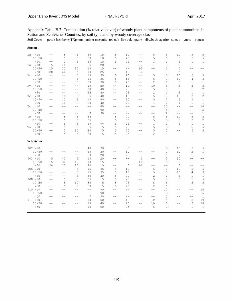
Upper Llano River EDYS Model FINAL REPORT April 2017
119
Appendix Table B.7 Composition (% relative cover) of woody plant components of plant communities in Sutton and Schleicher Counties, by soil type and by woody coverage class. Soil Cover pecan hackberry TXprsmn juniper mesquite red oak live oak grape elbwbush agarito sumac yucca pppear Sutton Es <10 -- 5 5 30 15 5 10 -- 5 5 10 5 5 10-50 -- 5 5 30 10 5 20 -- 5 5 5 5 5 >50 -- 2 2 45 15 5 25 -- 1 1 2 1 1 Fd <10 15 40 5 5 20 -- -- 5 -- 5 5 -- -- 10-50 15 30 10 10 15 -- -- 10 -- 5 5 -- -- >50 20 20 5 10 25 -- 10 5 -- -- 5 -- -- Kt <10 -- -- 5 15 35 5 10 -- 5 5 10 5 5 10-50 -- -- 5 15 35 5 15 -- 5 3 10 4 3 >50 -- -- 5 30 30 5 20 -- 2 1 5 1 1 Ky <10 -- -- -- 10 50 -- 10 -- 10 5 5 5 5 10-50 -- -- -- 20 40 -- 20 -- 5 3 5 5 2 >50 -- -- -- 25 40 -- 25 -- 2 1 5 1 1 Rc <10 -- 10 5 5 40 -- 15 -- 5 5 10 3 2 10-50 -- 10 5 10 40 -- 20 -- 5 2 5 2 1 >50 -- 10 5 20 40 -- 20 -- 1 1 1 1 1 Tc <10 -- -- -- -- 80 -- -- -- -- 10 -- -- 10 10-50 -- -- -- -- 90 -- -- -- -- 5 -- -- 5 >50 -- -- -- 7 90 -- -- -- -- 2 -- -- 1 Tr <10 -- 5 5 35 -- 5 20 -- 5 5 10 5 5 10-50 -- 5 5 35 -- 5 30 -- 5 5 5 3 2 >50 -- 1 3 60 -- 5 25 -- 1 1 2 1 1 Ts <10 -- 5 5 35 5 5 20 -- 5 5 5 5 5 10-50 -- 5 10 30 5 5 25 -- 5 5 -- 5 5 >50 -- 5 5 50 5 5 25 -- 2 1 -- 1 1 Schleicher 002 <10 -- -- -- 40 30 -- 5 -- -- 5 10 5 5 10-50 -- -- -- 45 30 -- 10 -- -- 2 10 2 1 >50 -- -- -- 50 20 -- 20 -- -- 1 7 1 1 003 <10 5 40 5 10 20 -- -- 5 -- 5 10 -- -- 10-50 15 30 10 10 15 -- -- 10 -- 5 5 -- -- >50 20 10 10 30 10 -- 5 10 -- -- 5 -- -- 005 <10 -- -- 5 15 35 5 10 -- 5 5 10 5 5 10-50 -- -- 5 15 35 5 15 -- 5 3 10 4 3 >50 -- -- 5 30 30 5 20 -- 2 1 5 1 1 008 <10 -- 5 5 35 5 5 20 -- 5 5 5 5 5 10-50 -- 5 10 30 5 5 25 -- 5 5 -- 5 5 >50 -- 5 5 50 5 5 25 -- 2 1 -- 1 1 010 <10 -- -- -- -- 80 -- -- -- -- 10 -- -- 10 10-50 -- -- -- -- 90 -- -- -- -- 5 -- -- 5 >50 -- -- -- 7 90 -- -- -- -- 2 -- -- 1 011 <10 -- -- -- 10 50 -- 10 -- 10 5 -- 5 10 10-50 -- -- -- 10 40 -- 20 -- 10 5 -- 5 10 >50 -- -- -- 15 50 -- 25 -- 5 3 -- 1 1
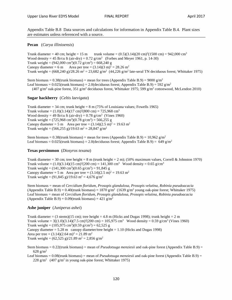
Upper Llano River EDYS Model FINAL REPORT April 2017
120
Appendix Table B.8 Data sources and calculations for information in Appendix Table B.4. Plant sizes are estimates unless referenced with a source. Pecan (Carya illinioensis) Trunk diameter = 40 cm; height = 15 m trunk volume = (0.5)(3.14)(20 cm)2(1500 cm) = 942,000 cm3 Wood density = 45 lb/cu ft (air-dry) = 0.72 g/cm3 (Forbes and Meyer 1961, p. 14-30) Trunk weight = (942,000 cm3)(0.72 g/cm3) = 668,240 g Canopy diameter = 6 m Area per tree = (3.14)(3 m)2 = 28.26 m2 Trunk weight = (668,240 g)/28.26 m2 = 23,682 g/m2 (44,226 g/m2 late-seral TN deciduous forest; Whittaker 1975) Stem biomass = 0.38(trunk biomass) = mean for trees (Appendix Table B.9) = 9000 g/m2 Leaf biomass = 0.025(trunk biomass) = 2.0(deciduous forest; Appendix Table B.9) = 592 g/m2 (407 g/m2 oak-pine forest, 351 g/m2 deciduous forest, Whittaker 1975; 599 g/m2 cottonwood, McLendon 2010) Sugar hackberry (Celtis laevigata) Trunk diameter = 34 cm; trunk height = 8 m (75% of Louisiana values; Fowells 1965) Trunk volume = (1.0)(3.14)(17 cm)2(800 cm) = 725,968 cm3 Wood density = 49 lb/cu ft (air-dry) = 0.78 g/cm3 (Vines 1960) Trunk weight = (725,968 cm3)(0.78 g/cm3) = 566,255 g Canopy diameter = 5 m Area per tree = (3.14)(2.5 m)2 = 19.63 m2 Trunk weight = (566,255 g)/19.63 m2 = 28,847 g/m2 Stem biomass = 0.38(trunk biomass) = mean for trees (Appendix Table B.9) = 10,962 g/m2 Leaf biomass = 0.025(trunk biomass) = 2.0(deciduous forest; Appendix Table B.9) = 649 g/m2 Texas persimmon (Diosyros texana) Trunk diameter = 30 cm; tree height = 8 m (trunk height = 2 m); (50% maximum values, Correll & Johnston 1970) Trunk volume = (1.0)(3.14)(15 cm)2(200 cm) = 141,300 cm3 Wood density = 0.65 g/cm3 Trunk weight = (141,300 cm3)(0.65 g/cm3) = 91,845 g Canopy diameter = 5 m Area per tree = (3.14)(2.5 m)2 = 19.63 m2 Trunk weight = (91,845 g)/19.63 m2 = 4,676 g/m2 Stem biomass = mean of Cercidium floridum, Prosopis glandulosa, Prosopis velutina, Robinia pseudoacacia (Appendix Table B.9) = 0.40(trunk biomass) = 1870 g/m2 (1639 g/m2 young oak-pine forest; Whittaker 1975) Leaf biomass = mean of Cercidium floridum, Prosopis glandulosa, Prosopis velutina, Robinia pseudoacacia (Appendix Table B.9) = 0.09(trunk biomass) = 421 g/m2 Ashe juniper (Juniperus ashei) Trunk diameter = (3 stems)(15 cm); tree height = 4.8 m (Hicks and Dugas 1998); trunk height = 2 m Trunk volume = 3[(1.0)(3.14)(7.5 cm)2(200 cm) = 105,975 cm3 Wood density = 0.59 g/cm3 (Vines 1960) Trunk weight = (105,975 cm3)(0.59 g/cm3) = 62,525 g Canopy diameter = 5.28 m canopy diameter/tree height = 1.10 (Hicks and Dugas 1998) Area per tree = (3.14)(2.64 m)2 = 21.89 m2 Trunk weight = (62,525 g)/21.89 m2 = 2,856 g/m2 Stem biomass = 0.22(trunk biomass) = mean of Pseudotsuga menziesii and oak-pine forest (Appendix Table B.9) = 628 g/m2 Leaf biomass = 0.08(trunk biomass) = mean of Pseudotsuga menziesii and oak-pine forest (Appendix Table B.9) = 228 g/m2 (407 g/m2 in young oak-pine forest; Whittaker 1975)

Upper Llano River EDYS Model FINAL REPORT April 2017
121
Appendix Table B.8 (Cont.) Mesquite (Prosopis glandulosa) Trunk diameter = (2 stems)(15 cm); tree height = 10 m (Vines 1960); trunk height = 3 m Trunk volume = (2)(3.14)(7.5 cm)2(300 cm) = 105,975 cm3 Wood density = 0.71 g/cm3 (Ayensu 1980) Trunk weight = (105,975 cm3)(0.71 g/cm3) = 75,242 g (75,920 g for P. velutina; Barth and Klemmedson 1982) Canopy diameter = 6 m Area per tree = (3.14)(3 m)2 = 28.26 m2 (20.9 m2 P. velutina; Barth & Klemmedson 1982) Trunk weight = (75,242 g)/28.26 m2 = 2,662 g/m2 (1,293 g/m2 for P. velutina; Barth & Klemmedson 1982) Stem biomass = 0.33(trunk biomass) = mean of P. glandulosa and P. velutina (Appendix Table B.9) = 878 g/m2 Leaf biomass = 0.14(trunk biomass) = mean of P. glandulosa and P. velutina (Appendix Table B.9) = 373 g/m2 Texas red oak (Quercus buckleyi) Trunk diameter = 20 cm; tree height = 10 m (Vines 1960); (tree height/trunk diameter = 24; Fowells 1965) Trunk volume = (0.5)(3.14)(10 cm)2(1000 cm) = 157,000 cm3 Wood density = 57 lb/cu ft (Vines 1960) = 0.91 g/cm3 Trunk weight = (157,000 cm3)(0.91 g/cm3) = 142,870 g Tree density = 175 trees/acre at 8-inch diameter trunks (Fowells 1965) Area per tree = 4047 m2/175 = 23.13 m2 Trunk weight = (142,870 g)/23.13 m2 = 6,177 g/m2 Stem biomass = 0.25(trunk biomass) = mean of oak-pine and deciduous forests (Appendix Table B.9) = 1544 g/m2 (1639 g/m2 young oak-pine forest, 6026 g/m2 late-seral TN deciduous forest; Whittaker 1975) Leaf biomass = 0.05(trunk biomass) = mean of oak-pine and deciduous forests (Appendix Table B.9) = 309 g/m2 (407 g/m2 young oak-pine forest, 351 g/m2 late-seral TN deciduous forest; Whittaker 1975) Live oak (Quercus virginiana) Trunk diameter = 20 cm; tree height = 10 m; trunk height = 3.5 m Trunk volume = (1.0)(3.14)(10 cm)2(350 cm) = 109,900 cm3 Wood density = 59 lb/cu ft (Vines 1960) = 0.94 g/cm3 Trunk weight = (109,900 cm3)(0.94 g/cm3) = 103,306 g Canopy diameter = 5.2 m (canopy diameter/trunk thickness = 26; Fowells 1965) Area per tree = (3.14)(2.6 m)2 = 21.23 m2 Trunk weight = (103,306 g)/21.23 m2 = 4,866 g/m2 Stem biomass = 0.25(trunk biomass) = mean of oak-pine and deciduous forests (Appendix Table B.9) = 1217 g/m2 Leaf biomass = 0.05(trunk biomass) = mean of oak-pine and deciduous forests (Appendix Table B.9) = 243 g/m2 Mustang grape (Vitis mustangensis) Trunk diameter = 10 cm (maximum of 15 cm; Vines 1960); vine length = 8 m (maximum of 40 ft; Vines 1960) Trunk volume = (0.5)(3.14)(5 cm)2(800 cm) = 31,400 cm3 Vine density = 0.3 g/cm3 Main vine weight = (31,400 cm3)(0.3 g/cm3) = 9,420 g Assume half the vine length is height and half is horizontal, along the tops of trees. Assume the area covered by the horizontal length of the vine is a rectangle with length = the horizontal length and width = (0.5)horizontal length. Area per vine = (4 m)(2 m) = 8 m2 Main vine weight = (9,420 g)/8 m2 = 1,178 g/m2 Stem biomass = 0.10(trunk biomass) = 118 g/m2 Leaf biomass = 0.30(trunk biomass) = mean of tree and shrub means (Appendix Table B.10) = 353 g/m2

Upper Llano River EDYS Model FINAL REPORT April 2017
122
Appendix Table B.8 (Cont.) Elbowbush (Forestiera pubescens) Trunk diameter = 5 cm (one-third of maximum; Vines 1960) Shrub height = 150 cm (one-third of maximum; Vines 1960; Scifres 1980) Trunk volume = (0.5)(3.14)(2.5 cm)2(150 cm) = 1,472 cm3 Wood density = 39 lb/cu ft (F. acuminata; Vines 1960) = 0.63 g/cm3 Trunk weight = (1,472 cm3)(0.63 g/cm3) = 927 g Canopy diameter = 1.5 m Area per shrub = (3.14)(0.75 m)2 = 1.76 m2 Trunk weight = 927 g/1.76 m2 = 527 g/m2 Stem biomass = 2.0(trunk biomass) = mean for shrubs (Appendix Table B.10) = 1054 g/m2 Leaf biomass = 0.51(trunk biomass) = mean for shrubs (Appendix Table B.10) = 268 g/m2 Agarito (Mahonia trifoliolata) Trunk diameter = 2.5 cm; shrub height = 150 cm (Scifres 1980) Trunk volume = (0.5)(3.14)(1.25 cm)2(150 cm) = 367 cm3 Wood density = 0.5 g/cm3 Trunk weight = (367 cm3)(0.5 g/cm3) = 184 g Canopy diameter = 100 cm Area per shrub = (3.14)(0.5 m)2 = 0.79 m2 Trunk weight = 184 g/0.79 m2 = 233 g/m2 Stem biomass = 1.20(trunk biomass) = Artemisia spinescens (Appendix Table B.10) = 280 g/m2 Leaf biomass = 0.51(trunk biomass) = mean for shrubs (Appendix Table B.10) = 119 g/m2 Sacahuista (Nolina texana) Stem diameter = 15 cm; stem height = 50 cm (Correll and Johnston 1970) Stem volume = (1.0)(3.14)(7.5 cm)2(50 cm) = 883 cm3 Stem density = 0.25 g/cm3 Stem weight = (883 cm3)(0.25 g/cm3) = 221 g Canopy diameter = 1.2 m Area per plant = (3.14)(0.6 m)2 = 1.13 m2 Stem weight = 221 g/1.13 m2 = 195 g/m2 Leaf biomass = 2.69(stem biomass) = Sporobolus airoides (McLendon 2010) = 525 g/m2 Evergreen sumac (Rhus virens) Trunk diameter = 5 cm; shrub height = 3.5 m (Vines 1960; Correll and Johnston 1970) Trunk volume = (0.5)(3.14)(2.5 cm)2(350 cm) = 3,434 cm3 Wood density = 32 lb/cu ft (R. copallina; Vines 1960) = 0.51 g/cm3 Trunk weight = (3,434 cm3)(0.51 g/cm3) = 1,751 g Canopy diameter = 2.5 m Area per plant = (3.14)(1.25 m)2 = 1.56 m2 Trunk weight = 1,751 g/1.56 m2 = 1,123 g/m2 Stem biomass = 1.15(trunk biomass) = mean of tree and shrub means (Appendix Table B.10) = 1291 g/m2 Leaf biomass = 0.30(trunk biomass) = mean of tree and shrub means (Appendix Table B.10) = 337 g/m2 Yucca (Yucca constricta) Stem diameter = 6 cm; stem height = 20 cm (Correll and Johnston 1970) Stem volume = (1.0)(3.14)(3 cm)2(20 cm) = 565 cm3 Pulp density = 0.25 g/cm3 (less than 0.29 g/cm3 for northern white cedar; Forbes and Meyer 1961) Stem weight = (565 cm3)(0.25 g/cm3) = 142 g Canopy diameter = 60 cm Area per plant = (3.14)(0.3 m)2 = 0.28 m2 Stem weight = 142 g/0.28 m2 = 504 g/m2 Leaf biomass = 1.60(stem biomass) = mean of shrub leaf/trunk (Appendix Table B.10) and Sporobolus airoides leaf/stem (McLendon 2010) = 806 g/m2

Upper Llano River EDYS Model FINAL REPORT April 2017
123
Appendix Table B.8 (Cont.) Prickly pear (Opuntia lindheimeri) Trunk diameter = 12 cm; trunk height = 50 cm (half of maximum; Vines 1960) Trunk volume = (1.0)(3.14)(6 cm)2(50 cm) = 5,652 cm3 Trunk density = 0.25 g/cm3 Trunk weight = (5,652 cm3)(0.25 g/cm2) = 1,413 g Patch diameter = 1.5 m Area per plant = (3.14)(0.75 m)2 = 2.36 m2 Trunk weight = (1,413 g)/2.36 m2 = 599 g/m2 Pads = 25 cm long and 20 cm wide (Correll and Johnston 1970) Stem (pad) biomass = 2.0(trunk biomass) = 1198 g/m2 Appendix Table B.9 Aboveground biomass allocations for trees. Species Biomass Proportion Reference Trunk Stems Twigs Leaves Trunk Stems Twigs Leaves Cercidium floridum 544 171 17 3 0.74 0.23 0.02 0.01 Barth & Klemmedson 1982 Populus fremontii 3075 745 1002 302 0.60 0.14 0.20 0.06 McLendon 2008 Prosopis glandulosa 304 186 24 88 0.50 0.31 0.04 0.15 Barth & Klemmedson 1982 Prosopis velutina 759 83 3 34 0.86 0.10 t 0.04 Barth & Klemmedson 1982 Pseudotsuga menziesii 2543 229 7 172 0.86 0.08 t 0.06 Gower et al. 1992 Quercus gambelii 1573 985 775 --- McLendon et al. 1999 Robinia pseudoacacia 1373 553 364 108 0.57 0.23 0.15 0.05 McLendon 2008 Salix laevigata 597 281 363 150 0.43 0.20 0.26 0.11 McLendon 2008 Oak-pine forest NY 4317 1639 --- 407 0.68 0.26 ---- 0.06 Whittaker 1975 Deciduous forest TN 4427 603 --- 35 0.87 0.12 ---- 0.01 Whittaker 1975 MEAN 0.68 -- 0.26 -- 0.06
Biomass units vary among species but are constant within species.

Upper Llano River EDYS Model FINAL REPORT April 2017
124
Appendix Table B.10 Aboveground biomass allocations for shrubs. Species Biomass Proportion Reference Trunk Stems Twigs Leaves Trunk Stems Twigs Leaves Ambrosia dumosa 34 139 33 20 0.15 0.61 0.15 0.09 McLendon 2010 Artemisia spinescens 57 54 17 14 0.40 0.38 0.12 0.10 McLendon 2010 Artemisia tridentata 270 1411 --- 124 0.15 -- 0.78 -- 0.07 McLendon (unpublished) Artemisia tridentata 488 754 280 249 0.27 0.43 0.16 0.14 McLendon 2010 Artemisia tridentata -- 760 -- 74 178 -- 0.75 -- 0.08 0.17 Sturges 1977 Artemisia tridentata -- 272 -- --- 65 0.19 Uresk et al. 1977 Atriplex canescens 181 311 98 121 0.25 0.44 0.14 0.17 McLendon 2010 Atriplex confertifolia -- 339 -- 23 99 -- 0.74 -- 0.05 0.21 Caldwell et al. 1977 Atriplex confertifolia 70 90 129 56 0.20 0.26 0.38 0.16 McLendon 2010 Atriplex torreyi 435 804 501 862 0.17 0.31 0.19 0.33 McLendon 2008 Atriplex torreyi 238 347 227 220 0.23 0.34 0.22 0.21 McLendon 2010 Ceratoides lanata -- 161 -- 9 32 -- 0.80 -- 0.04 0.16 Caldwell et al. 1977 Chrysothamnus nauseosus 134 360 259 74 0.16 0.44 0.31 0.09 McLendon 2010 Ephedra nevadensis 82 119 54 0 0.32 0.47 0.21 0.00 McLendon 2010 Hymenoclea salsola 138 123 82 98 0.31 0.28 0.19 0.22 McLendon 2010 Psorothamnus arborescens 477 639 151 111 0.35 0.46 0.11 0.08 McLendon 2010 Quercus havardii --- 699 --- 380 0.35 Sears et al. 1986 Rosa woodsii 214 83 15 51 0.59 0.23 0.04 0.14 McLendon 2010 Salix exigua 310 256 54 64 0.45 0.38 0.08 0.09 McLendon et al. 1999 Salix exigua 217 201 40 39 0.44 0.40 0.08 0.08 McLendon 2010 Sarcobatus vermiculatus 260 403 433 228 0.20 0.30 0.33 0.17 McLendon 2010 Suaeda moquinii 59 95 47 86 0.21 0.33 0.16 0.30 McLendon 2010 Tetradymia axillaris 128 214 154 15 0.25 0.42 0.30 0.03 McLendon 2010 Mean of Observations 0.28 0.39 0.17 0.16 Mean of Species 0.29 0.39 0.17 0.15
Biomass units vary among species but are constant within species. Appendix Table B.11 Species composition and initial biomass values for land-use types in the Upper Llano River Watershed models. Values for woody species are in % of total woody cover and impervious surfaces are in % of total area. Values for herbaceous species are g/m2. Species Urban Buildings Disturbed Gravel Tilled Orchard Brush Houses Industrial Areas Pits Fields Control Pecan 0 0 0 0 0 100 0 Ashe juniper 0 0 24 30 0 0 30 Mesquite 25 50 24 25 0 0 25 Live oak 75 0 2 5 0 0 5 Elbowbush 0 0 0 0 0 0 5 Evergreen sumac 0 50 50 40 0 0 30 Prickly pear 0 0 0 0 0 0 5 Purple threeawn 0 10 20 10 0 0 3 Cane bluestem 0 10 5 20 0 0 4 King Ranch bluestem 0 30 20 10 0 5 2 Sideoats grama 0 0 0 0 0 0 5 Red grama 0 5 5 10 0 0 3 Bermudagrass 150 0 0 0 0 75 0 Sand dropseed 0 5 10 5 0 0 3 Wheat 0 0 0 0 20 0 0 Ragweed 0 30 40 20 0 5 15 Sunflower 0 20 30 20 10 5 10 Impervious surface 50% 50% 0% 75% 0% 0% 0%
To determine biomass of woody species, multiply the percent cover by species (Appendix Table B.18) by the percent total woody plant cover, by the biomass values in Appendix Table B.7.

Upper Llano River EDYS Model FINAL REPORT April 2017
125
Appendix Table B.12 Effect of woody cover on grass production on two rangelands in Texas. Mesquite Canopy (%) Huisache Canopy (%) 2- 3 7- 8 13 24 00 10 20 30 40 50 60 70 Production (g/m2): 126 135 145 96 415 425 365 320 290 235 190 135 Proportion of 2-3% canopy: 1.00 1.07 1.15 0.76 1.00 1.02 0.88 0.77 0.70 0.57 0.46 0.33 Mesquite = Rolling Plains near Vernon (McDaniel et al. 1982); huisache = Welder Wildlife Refuge, San Patricio County (Scifres et al. 1982). Approximate grass production = (amount at 0% cover)[1.00 – (0.8)(woody plant cover)]

Upper Llano River EDYS Model FINAL REPORT April 2017
126
APPENDIX C PLANT PARAMETERS Appendix Table C.1 General characteristics for species used in the Upper Llano River EDYS models. Species Growth Form Legume Biennial Pecan deciduous tree 0 no Sugar hackberry deciduous tree 0 no Texas persimmon deciduous tree 0 no Ashe juniper evergreen tree 0 no Mesquite deciduous tree 1 no Texas red oak deciduous tree 0 no Live oak evergreen tree 0 no Prairie baccharis deciduous shrub 0 no Elbowbush deciduous shrub 0 no Agarito evergreen shrub 0 no Sacahuista evergreen shrub 0 no Evergreen sumac evergreen shrub 0 no Yucca evergreen shrub 0 no Mustang grape deciduous vine 0 no Prickly pear cacti 0 no Giant cane perennial grass 0 no Purple threeawn perennial grass 0 no Cane bluestem perennial grass 0 no King Ranch bluestem perennial grass 0 no Sideoats grama perennial grass 0 no Hairy grama perennial grass 0 no Red grama perennial grass 0 no Bermudagrass perennial grass 0 no Canada wildrye perennial grass 0 no Plains lovegrass perennial grass 0 no Texas cupgrass perennial grass 0 no Curly mesquite perennial grass 0 no Green sprangletop perennial grass 0 no Vine-mesquite perennial grass 0 no Switchgrass perennial grass 0 no Little bluestem perennial grass 0 no Indiangrass perennial grass 0 no Johnsongrass perennial grass 0 no Tall dropseed perennial grass 0 no Sand dropseed perennial grass 0 no Texas wintergrass perennial grass 0 no Wheat annual grass 0 no Flatsedge perennial grass-like 0 no Spikerush perennial grass-like 0 no Bulrush perennial grass-like 0 no Cattail perennial grass-like 0 no Ragweed perennial forb 0 no Lazydaisy perennial forb 0 no Bundleflower perennial forb 1 no Indian blanket perennial forb 0 no Sunflower annual forb 0 no Duckweed annual forb 0 no Texas bluebonnet annual forb 1 no Prairie coneflower perennial forb 0 no Bush sunflower perennial forb 0 no Orange zexmenia perennial forb 0 no

Upper Llano River EDYS Model FINAL REPORT April 2017
127
Appendix Table C.2 Tissue allocation in mature plants, by plant part (proportion of total), and root:shoot ratio (R:S) for species included in the Upper Llano River EDYS model. Species Coarse Roots Fine Roots Trunk Stems Leaves Seeds R:S Ratio Pecan 0.32 0.11 0.40 0.12 0.05 0.00 0.75 Sugar hackberry 0.16 0.06 0.55 0.17 0.06 0.00 0.28 Texas persimmon 0.32 0.11 0.40 0.12 0.05 0.00 0.75 Ashe juniper 0.15 0.05 0.56 0.18 0.06 0.00 0.25 Mesquite 0.14 0.10 0.39 0.28 0.09 0.00 0.32 Texas red oak 0.20 0.07 0.51 0.16 0.06 0.00 0.36 Live oak 0.24 0.08 0.48 0.15 0.05 0.00 0.46 Prairie baccharis 0.26 0.12 0.34 0.19 0.09 0.00 0.61 Elbowbush 0.28 0.12 0.33 0.18 0.09 0.00 0.66 Agarito 0.35 0.14 0.28 0.15 0.08 0.00 0.97 Sacahuista 0.29 0.13 0.32 0.08 0.18 0.00 0.73 Evergreen sumac 0.32 0.14 0.30 0.16 0.08 0.00 0.84 Yucca 0.35 0.15 0.27 0.12 0.11 0.00 1.00 Mustang grape 0.23 0.10 0.35 0.17 0.15 0.00 0.50 Prickly pear 0.16 0.08 0.37 0.38 0.01 0.00 0.31 Giant cane 0.18 0.18 0.18 0.26 0.20 0.00 0.36 Purple threeawn 0.33 0.32 0.07 0.14 0.14 0.00 1.89 Cane bluestem 0.31 0.31 0.08 0.15 0.15 0.00 1.60 King Ranch bluestem 0.31 0.30 0.08 0.16 0.15 0.00 1.59 Sideoats grama 0.31 0.31 0.08 0.15 0.15 0.00 1.60 Hairy grama 0.18 0.18 0.21 0.06 0.37 0.00 0.56 Red grama 0.18 0.18 0.21 0.06 0.37 0.00 0.56 Bermudagrass 0.28 0.27 0.15 0.05 0.25 0.00 1.21 Canada wildrye 0.31 0.31 0.08 0.15 0.15 0.00 1.65 Plains lovegrass 0.18 0.18 0.13 0.26 0.25 0.00 0.58 Texas cupgrass 0.26 0.26 0.10 0.19 0.19 0.00 1.06 Curly mesquite 0.40 0.26 0.11 0.03 0.20 0.00 1.98 Green sprangletop 0.23 0.23 0.11 0.22 0.21 0.00 0.86 Vine-mesquite 0.23 0.23 0.11 0.22 0.21 0.00 0.85 Switchgrass 0.25 0.25 0.10 0.20 0.20 0.00 0.98 Little bluestem 0.31 0.31 0.08 0.15 0.15 0.00 1.63 Indiangrass 0.37 0.36 0.05 0.11 0.11 0.00 0.86 Johnsongrass 0.35 0.34 0.06 0.13 0.12 0.00 2.21 Tall dropseed 0.26 0.26 0.10 0.19 0.19 0.00 1.10 Sand dropseed 0.24 0.23 0.11 0.21 0.21 0.00 0.88 Texas wintergrass 0.28 0.28 0.13 0.04 0.27 0.00 1.26 Wheat 0.23 0.24 0.11 0.21 0.21 0.00 0.88 Flatsedge 0.39 0.38 0.05 0.09 0.09 0.00 3.33 Spikerush 0.41 0.41 0.04 0.13 0.01 0.00 4.62 Bulrush 0.39 0.38 0.05 0.09 0.09 0.00 3.33 Cattail 0.39 0.38 0.05 0.09 0.09 0.00 3.33 Ragweed 0.28 0.28 0.09 0.18 0.17 0.00 1.26 Lazydaisy 0.29 0.29 0.08 0.17 0.17 0.00 1.38 Bundleflower 0.29 0.30 0.08 0.16 0.17 0.00 1.46 Indian blanket 0.29 0.29 0.08 0.17 0.17 0.00 1.38 Sunflower 0.08 0.07 0.17 0.34 0.34 0.00 0.17 Duckweed 0.12 0.11 0.15 0.31 0.31 0.00 0.30 Texas bluebonnet 0.20 0.20 0.12 0.24 0.24 0.00 0.66 Prairie coneflower 0.29 0.29 0.08 0.18 0.17 0.00 1.38 Bush sunflower 0.28 0.28 0.09 0.18 0.17 0.00 1.26 Orange zexmenia 0.28 0.28 0.09 0.18 0.17 0.00 1.26

Upper Llano River EDYS Model FINAL REPORT April 2017
128
Data Sources (Appendix Table C.2) Root:Shoot Ratios Pecan: slow-growing hardwoods (Odum 1971:375) Sugar hackberry : Fagus sp. (Garelkov 1973) Texas persimmon: slow-growing hardwoods (Odum 1971:375) Ashe juniper: Juniperus osteosperma (McLendon unpublished data) Mesquite: [twice the value reported by Barth et al. (1982) + mean(control and natural)Ansley et al. 2014]/2 Texas red oak: Mean of Quercus alba (Nadelhoffer et al. 1985), Q. rubra (Nadelhoffer et al. 1985), Q. robur (Andersson 1970, Duvigneaud et al. 1971, Rodin & Bazilevich 1967), Q. robus (Duvigneaud et al. 1971), Q. velutina (Nadelhoffer et al. 1985) Live oak: Mean of Quercus alba and Q. velutina (Nadelhoffer et al. 1985) Elbowbush: Mean of Arctostaphylos pungens (Kummerow et al.1977), Cornus florida (Blair 1982), Fallugia paradoxa (Ludwig 1977), Flourensia cernua (Ludwig 1977), Grayia spinosa (Wallace et al. 1974), Ilex vomitoria (Blari 1982), Krameria parvifolia (Wallace et al. 1974), Lycium andersonii (Wallace et al. 1974) Sacahuista: Dasylirion-Bouteloua shrubland, Big Bend NP (McLendon, unpublished data) Evergreen sumac: Mean of Cornus florida (Blair 1982), Ilex vomitoria (Blair 1982), Salix exigua (Evans et al. 2013) Yucca: Yucca elata (Ludwig 1977) Prickly pear: Opuntia lindheimeri Big Bend NP (McLendon, unpublished data) Giant cane: Typha angustifolia (Shipley & Peters 1990) Purple threeawn: Briske et al. (1996), Fernandez & Reynolds (2000), McLendon (unpublished), Vinton & Burke (1995) Cane bluestem: Bouteloua curtipendula (Scifres & Halifax 1972; McLendon unpublished) KR bluestem: Coyne and Bradford (1986) Sideoats grama: Scifres and Halifax (1972); McLendon (unpublished field data from Big Bend NP) Hairy grama: Bouteloua rigidiseta (Briske et al. 1996) Red grama: Bouteloua rigidiseta (Briske et al. 1996) Bermudagrass: Beaty et al. (1973), Guglielmini & Satorre (2002), Hons et al. (1979), Huang et al. (1997), Impithuksa et al. (1979), Rodriguez et al. (2002), Stoddart et al. (1975:136) Canada wildrye: Mean of Elymus cinereus (Blank & Young 1998), E. lanceolatus (Aguirre & Johnson 1991), E. triticoides (Evans et al. 2013) Plains lovegrass: Mean of Eragrostis curvula (Masters & Britton 1990), E. lehmanniana (Fernandez & Reynolds 2000) Texas cupgrass: Mean of Agropyron inerme (Mack 1986:151), Agrostis scabra (Tilman & Wedin 1991), Dactylis glomerata (Davidson 1969) Curly mesquite: Buchloe dactyloides (McLendon, unpublished data) Green sprangletop: Mean of Agropyron repens (Tilman & Wedin 1991), Agrostis scabra (Tilman & Wedin 1991), Calamagrostis rubescens (Stourt et al. 1983), Festuca ovina (Whittingham & Reed 1982), Hyparrhenia rufa (Peters & Baruch 1997), Poa pratensis (Tilman & Wedin 1991), Sporobolus cryptandrus (Paschke et al. 2000) Vine-mesquite: Fernandez and Reynolds (2000) Switchgrass: Brejda et al. (1993); Johnson (1998); Scifres and Halifax (1972) Little bluestem: Tilman and Wedin (1991) Indiangrass: Mean of Andropogon gerardii (Tilman & Wedin 1991), Panicum virgatum (Brejda et al.1993) Johnsongrass: Mean of Andropogon gerardii (Tilman & Wedin 1991), Bothriochloa caucasica (Coyne & Bradford 1986), Bouteloua curtipendula (McLendon, unpublished), Bromus inermis (McLendon et al. 1999, Johnson 2005), Elymus triticoides (Evans et al. 2013), Festuca arundinacea (Overman 1995), Panicum virgatum (Brejda et al. 1993), Paspalum notatum (Hons et al. 1979, Impithuksa et al. 1979, Fiala et al. 1991) Tall dropseed: Sporobolus flexuosus (Fernandez & Reynolds 2000) Sand dropseed: Paschke et al. (2000)

Upper Llano River EDYS Model FINAL REPORT April 2017
129
Texas wintergrass: Stipa comata (Vinton & Burke 1995; Burleson & Hewitt 1982) Wheat: Buyanovsky et al. (1987) Flatsedge: Mean of Carex acutiformis (Aerts & de Caluwe 1994), C. diandra (Aerts & de Caluwe 1994), C. douglasii (Manning et al. 1989), C. nebrascensis (Manning et al. 1989), C. rostrata (Aerts & de Caluwe 1994), Juncus roemerianus (Gallagher et al. 1977) Spikerush: Juncus balticus (Evans et al. 2013; Manning et al. 1989) Bulrush: Same as flatsedge. Cattail: Same as flatsedge. Ragweed: Mean of Centaurea maculosa (Olson & Wallander 1997; Velagala et al. 1997), Centaurea repens (Lowe et al. 2002), Parthenium incanum (Ludwig 1977) and Rumex acetosa (Gigon & Rorison 1972) Lazydaisy: Mean of Salvia mellifera (Hellmers et al. 1955), Verbascum thapsus (McLendon unpublished) Bundleflower: Mean of Astragalus micropterus (Barbour 1973), Hedysarum borale (Johnson et al. 1989) Indian blanket: Same as lazydaisy. Sunflower: Goodman and Ennos (1999) Duckweed: Mean of Leersia oryzoides (Shipley & Peters 1990) and Zizania aquatica (Bray 1963) Texas bluebonnet: Mean of Trifolium repens (Davidson 1969; Haystead et al. 1988; McNeill & Wood 1990) and T. subterraneum (Smith 1982) Prairie coneflower: Same as lazydaisy. Bush sunflower: Same as ragweed. Orange zexmenia: Same as ragweed. Aboveground Tissue Allocation (Trunk:Stem:Leaves) Trees: 0.70:0.22:0.08 Shrubs: 0.55:0.30:0.15 Herbaceous (stemmy): 0.2:0.4:0.4 Herbaceous (short): 0.3:0.1:0.6
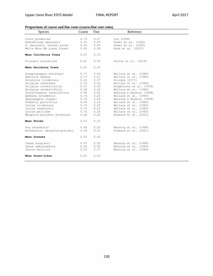
Upper Llano River EDYS Model FINAL REPORT April 2017
130
Proportions of coarse and fine roots (coarse;fine root ratio). Species Coarse Fine Reference Pinus ponderosa 0.73 0.27 Cox (1958) Pseudotsuga menziesii 0.91 0.09 Gower et al. (1992) P. menziesii (annual prod) 0.40 0.60 Gower et al. (1992) White Mtns NH young forest 0.62 0.38 Park et al. (2007) Mean Coniferous Trees 0.67 0.33 Prosopis glandulosa 0.61 0.39 Ansley et al. (2014) Mean Deciduous Trees 0.61 0.39 Acamptopappus shockleyi 0.77 0.23 Wallace et al. (1980) Ambrosia dumosa 0.73 0.27 Wallace et al. (1980) Artemisia tridentata 0.63 0.37 Sturges (1977) Atriplex canescens 0.70 0.30 Wallace et al. (1980) Atriplex confertifolia 0.07 0.93 Hodgkinson et al. (1978) Atriplex confertifolia 0.68 0.32 Wallace et al. (1980) Chrysothamnus teretifolius 0.98 0.02 Manning & Barbour (1988) Ephedra nevadensis 0.76 0.24 Wallace et al. (1980) Haplopappus cooperi 0.76 0.24 Manning & Barbour (1988) Krameria parvifolia 0.64 0.36 Wallace et al. (1980) Larrea tridentata 0.75 0.25 Wallace et al. (1980) Lycium andersonii 0.75 0.25 Wallace et al. (1980) Lycium pallidum 0.74 0.26 Wallace et al. (1980) Mesquite-granjeno shrubland 0.40 0.60 Hibbard et al. (2001) Mean Shrubs 0.67 0.33 Poa nevadensis 0.48 0.52 Manning et al. (1989) Herbaceous, mesquite-granjeno 0.59 0.41 Hibbard et al. (2001) Mean Grasses 0.54 0.46 Carex douglasii 0.47 0.53 Manning et al. (1989) Carex nebrascensis 0.42 0.58 Manning et al. (1989) Juncus balticus 0.53 0.47 Manning et al. (1989) Mean Grass-Likes 0.47 0.53

Upper Llano River EDYS Model FINAL REPORT April 2017
131
Appendix Table C.3 Allocation of new biomass production by plant part (proportion of total) for species included in the Upper Llano River EDYS models. Species Coarse Roots Fine Roots Trunk Stems Leaves Seeds Pecan 0.11 0.32 0.15 0.08 0.34 0.00 Sugar hackberry 0.06 0.16 0.27 0.08 0.43 0.00 Texas persimmon 0.11 0.32 0.20 0.06 0.31 0.00 Ashe juniper 0.08 0.30 0.11 0.20 0.31 0.00 Mesquite 0.08 0.30 0.12 0.19 0.31 0.00 Texas red oak 0.07 0.20 0.25 0.08 0.40 0.00 Live oak 0.10 0.20 0.15 0.07 0.48 0.00 Prairie baccharis 0.05 0.20 0.05 0.20 0.50 0.00 Elbowbush 0.06 0.23 0.08 0.16 0.47 0.00 Agarito 0.07 0.25 0.10 0.10 0.48 0.00 Sacahuista 0.10 0.24 0.02 0.04 0.60 0.00 Evergreen sumac 0.08 0.25 0.10 0.15 0.42 0.00 Yucca 0.08 0.24 0.02 0.05 0.61 0.00 Mustang grape 0.03 0.20 0.10 0.15 0.52 0.00 Prickly pear 0.10 0.22 0.20 0.46 0.02 0.00 Giant cane 0.15 0.25 0.10 0.20 0.30 0.00 Purple threeawn 0.12 0.25 0.08 0.10 0.45 0.00 Cane bluestem 0.12 0.24 0.05 0.25 0.34 0.00 King Ranch bluestem 0.12 0.25 0.10 0.05 0.48 0.00 Sideoats grama 0.12 0.24 0.05 0.26 0.33 0.00 Hairy grama 0.09 0.18 0.10 0.06 0.57 0.00 Red grama 0.10 0.25 0.08 0.10 0.47 0.00 Bermudagrass 0.12 0.25 0.10 0.05 0.48 0.00 Canada wildrye 0.12 0.23 0.05 0.30 0.30 0.00 Plains lovegrass 0.12 0.24 0.08 0.25 0.31 0.00 Texas cupgrass 0.12 0.23 0.10 0.24 0.31 0.00 Curly mesquite 0.16 0.27 0.10 0.12 0.35 0.00 Green sprangletop 0.12 0.24 0.08 0.25 0.31 0.00 Vine-mesquite 0.11 0.21 0.06 0.30 0.32 0.00 Switchgrass 0.11 0.24 0.06 0.25 0.34 0.00 Little bluestem 0.13 0.25 0.05 0.26 0.31 0.00 Indiangrass 0.10 0.24 0.05 0.30 0.31 0.00 Johnsongrass 0.12 0.23 0.05 0.30 0.30 0.00 Tall dropseed 0.11 0.24 0.05 0.30 0.30 0.00 Sand dropseed 0.12 0.24 0.06 0.30 0.28 0.00 Texas wintergrass 0.10 0.20 0.05 0.40 0.25 0.00 Wheat 0.25 0.25 0.10 0.20 0.20 0.00 Flatsedge 0.18 0.35 0.06 0.12 0.29 0.00 Spikerush 0.16 0.30 0.06 0.48 0.00 0.00 Bulrush 0.18 0.20 0.06 0.25 0.31 0.00 Cattail 0.20 0.20 0.04 0.28 0.28 0.00 Ragweed 0.15 0.20 0.10 0.30 0.25 0.00 Lazydaisy 0.10 0.25 0.10 0.15 0.40 0.00 Bundleflower 0.08 0.18 0.10 0.32 0.32 0.00 Indian blanket 0.10 0.20 0.10 0.16 0.44 0.00 Sunflower 0.12 0.20 0.10 0.30 0.23 0.05 Duckweed 0.16 0.17 0.20 0.07 0.40 0.00 Texas bluebonnet 0.16 0.17 0.20 0.07 0.40 0.00 Prairie coneflower 0.12 0.24 0.08 0.30 0.26 0.00 Bush sunflower 0.12 0.25 0.12 0.26 0.25 0.00 Orange zexmenia 0.13 0.25 0.12 0.25 0.25 0.00

Upper Llano River EDYS Model FINAL REPORT April 2017
132
Appendix Table C.4 Allocation of biomass production in green-out months by plant part (proportion of total) for species included in the Upper Llano EDYS model. Species Coarse Roots Fine Roots Trunks Stems Leaves Seeds Pecan 0.00 0.24 0.00 0.05 0.71 0.00 Sugar hackberry 0.00 0.12 0.00 0.06 0.82 0.00 Texas persimmon 0.00 0.24 0.00 0.05 0.71 0.00 Ashe juniper 0.00 0.23 0.00 0.15 0.62 0.00 Mesquite 0.00 0.15 0.00 0.10 0.75 0.00 Texas red oak 0.00 0.15 0.00 0.06 0.79 0.00 Live oak 0.00 0.18 0.00 0.05 0.77 0.00 Prairie baccharis 0.00 0.19 0.00 0.20 0.61 0.00 Elbowbush 0.00 0.17 0.00 0.42 0.41 0.00 Agarito 0.00 0.26 0.00 0.37 0.37 0.00 Sacahuista 0.00 0.18 0.00 0.41 0.41 0.00 Evergreen sumac 0.00 0.19 0.00 0.41 0.40 0.00 Yucca 0.00 0.18 0.00 0.41 0.41 0.00 Mustang grape 0.00 0.17 0.00 0.23 0.60 0.00 Prickly pear 0.10 0.15 0.05 0.69 0.01 0.00 Giant cane 0.02 0.19 0.00 0.40 0.41 0.00 Purple threeawn 0.00 0.19 0.00 0.03 0.78 0.00 Cane bluestem 0.00 0.18 0.00 0.41 0.41 0.00 King Ranch bluestem 0.01 0.19 0.00 0.04 0.76 0.00 Sideoats grama 0.01 0.18 0.00 0.41 0.40 0.00 Hairy grama 0.00 0.14 0.00 0.03 0.83 0.00 Red grama 0.00 0.19 0.00 0.05 0.76 0.00 Bermudagrass 0.01 0.19 0.00 0.03 0.77 0.00 Canada wildrye 0.00 0.17 0.00 0.41 0.42 0.00 Plains lovegrass 0.00 0.18 0.00 0.41 0.41 0.00 Texas cupgrass 0.00 0.17 0.00 0.42 0.41 0.00 Curly mesquite 0.00 0.20 0.00 0.09 0.71 0.00 Green sprangletop 0.00 0.18 0.00 0.41 0.41 0.00 Vine-mesquite 0.01 0.16 0.00 0.15 0.68 0.00 Switchgrass 0.00 0.18 0.00 0.41 0.41 0.00 Little bluestem 0.01 0.18 0.00 0.40 0.41 0.00 Indiangrass 0.01 0.18 0.00 0.41 0.40 0.00 Johnsongrass 0.01 0.17 0.00 0.41 0.41 0.00 Tall dropseed 0.00 0.18 0.00 0.41 0.41 0.00 Sand dropseed 0.00 0.18 0.00 0.41 0.41 0.00 Texas wintergrass 0.00 0.19 0.00 0.03 0.78 0.00 Wheat 0.25 0.25 0.10 0.20 0.20 0.00 Flatsedge 0.00 0.26 0.00 0.20 0.54 0.00 Spikerush 0.00 0.22 0.00 0.78 0.00 0.00 Bulrush 0.02 0.15 0.00 0.42 0.41 0.00 Cattail 0.02 0.15 0.00 0.43 0.40 0.00 Ragweed 0.00 0.15 0.00 0.43 0.42 0.00 Lazydaisy 0.00 0.19 0.00 0.41 0.40 0.00 Bundleflower 0.00 0.14 0.00 0.43 0.43 0.00 Indian blanket 0.00 0.15 0.00 0.43 0.42 0.00 Sunflower 0.16 0.17 0.13 0.27 0.27 0.00 Duckweed 0.16 0.17 0.20 0.07 0.40 0.00 Texas bluebonnet 0.16 0.17 0.20 0.07 0.40 0.00 Prairie coneflower 0.00 0.18 0.00 0.41 0.41 0.00 Bush sunflower 0.00 0.19 0.00 0.41 0.40 0.00 Orange zexmenia 0.00 0.19 0.00 0.41 0.40 0.00

Upper Llano River EDYS Model FINAL REPORT April 2017
133
General guidelines for greenout allocation (Appendix Table. C.4): Trees: coarse roots, trunks, and seeds = no allocation; fine roots and stems = 75% of new growth allocation; leaves = remainder of allocation. Shrubs, midgrasses, and perennial forbs: coarse roots, trunks, and seeds = no allocation; fine roots = 75% of new growth allocation; stems + leaves = remainder of allocation (exception = rhizomatous grasses, which have coarse roots = 10% of new growth allocation). Shortgrasses = coarse roots, trunks, and seeds = no allocation; fine roots = 75% of new growth allocation; stems = 50% of new growth allocation; leaves = remainder of allocation (exceptions = rhizomatous grasses which have coarse roots = 10% of new growth allocation and stoloniferous grasses which have stems = 75% of new growth allocation). Annuals = new growth allocation.

Upper Llano River EDYS Model FINAL REPORT April 2017
134
Appendix Table C.9 Root architecture (percent of root biomass by percent of maximum rooting depth) and maximum potential rooting depth (mm) for plant species included in the Upper Llano EDYS model. Species Percent of Root Biomass by Percent of Maximum Rooting Depth Maximum 00-01 01-05 05-10 10-20 20-30 30-40 40-50 50-60 60-70 70-80 80-90 90-100 Rooting Depth Pecan 2 9 14 20 15 5 6 6 2 6 8 7 6250 Sugar hackberry 2 9 14 20 15 5 6 6 2 6 8 7 6000 Texas persimmon 2 9 14 20 15 5 6 6 2 6 8 7 5300 Ashe juniper 1 6 9 14 14 14 13 9 9 5 3 3 8000 Mesquite 14 14 20 15 9 7 6 5 4 3 2 1 53400 Texas red oak 4 14 15 21 12 8 8 7 4 4 2 1 7000 Live oak 4 14 15 21 12 8 8 7 4 4 2 1 22000 Prairie baccharis 1 5 9 12 18 17 11 11 7 6 2 1 1900 Elbowbush 3 13 14 17 14 12 9 6 5 4 2 1 2400 Agarito 3 10 12 19 13 12 10 9 5 4 2 1 3000 Sacahuista 2 9 10 17 14 11 8 7 10 6 4 2 990 Evergreen sumac 2 9 14 20 15 5 6 6 2 6 8 7 3530 Yucca 2 9 10 17 14 11 8 7 10 6 4 2 1400 Mustang grape 5 12 15 17 13 11 9 7 5 3 2 1 3660 Prickly pear 2 9 12 19 13 20 11 6 4 2 1 1 840 Giant cane 2 9 11 23 9 9 8 8 7 6 5 3 3500 Purple threeawn 4 14 16 18 18 12 6 4 4 2 1 1 1830 Cane bluestem 10 22 20 20 10 6 3 3 2 2 1 1 2380 KR bluestem 4 16 21 18 14 8 6 4 3 2 2 2 1200 Sideoats grama 10 20 23 21 14 5 2 1 1 1 1 1 3960 Hairy grama 5 13 14 18 13 11 9 9 4 2 1 1 1070 Red grama 4 13 14 20 13 10 9 7 4 3 2 1 600 Bermudagrass 5 14 17 15 12 10 8 6 5 4 3 1 900 Canada wildrye 4 12 16 18 14 12 8 6 4 3 2 1 720 Plains lovegrass 3 9 11 19 14 12 10 7 6 4 4 1 1200 Texas cupgrass 4 15 17 19 12 7 7 5 4 4 4 3 1040 Curly mesquite 5 15 16 18 11 10 9 4 4 3 3 2 1700 Green sprangletop 3 13 15 18 13 11 9 6 4 4 3 1 1150 Vine-mesquite 3 11 13 19 14 10 8 6 5 4 4 3 2020 Switchgrass 9 17 23 12 10 8 7 6 4 3 2 1 3350 Little bluestem 8 22 25 18 8 5 4 3 3 2 1 1 2440 Indiangrass 6 25 21 15 10 7 5 4 3 2 1 1 2430 Johnsongrass 3 12 17 18 14 10 9 7 5 3 1 1 2410 Tall dropseed 4 15 17 20 11 8 6 5 5 4 4 1 2130 Sand dropseed 6 19 19 27 9 4 3 3 3 3 2 2 2700 Texas wintergrass 3 11 13 18 14 10 8 8 6 4 3 2 1950 Wheat 2 5 7 15 16 15 13 10 8 5 3 1 3000 Flatsedge 2 5 8 15 13 12 12 10 9 7 4 3 630 Spikerush 5 10 15 30 16 5 5 3 3 3 3 2 700 Bulrush 1 2 5 12 13 13 12 12 12 9 6 3 600 Cattail 3 12 13 18 10 9 8 8 7 6 4 2 1400 Ragweed 6 20 20 27 10 4 3 3 2 2 2 1 1830 Lazydaisy 2 5 8 13 12 11 11 12 10 7 5 4 600 Bundleflower 3 9 14 23 12 5 4 5 9 7 6 3 2100 Indian blanket 1 7 10 17 17 14 10 7 7 6 3 1 2070 Sunflower 6 24 6 9 12 16 10 7 2 3 3 2 3100 Duckweed 1 4 7 15 15 13 10 10 12 8 4 1 110 Texas bluebonnet 2 9 14 37 16 5 3 3 3 2 2 4 1040 Prairie coneflower 4 16 14 23 14 6 6 4 4 4 3 2 1830 Bush sunflower 4 14 18 29 11 6 5 4 3 3 2 1 2620 Orange zexmenia 3 8 13 30 11 8 7 7 5 4 3 1 2640

Upper Llano River EDYS Model FINAL REPORT April 2017
135
Data Sources (Appendix Table C.9) Root Architecture Pecan, sugar hackberry, Texas persimmon: Acer saccharum (Dawson 1993) Ashe juniper: Juniperus occidentalis (Young & Evans 1986) Mesquite: mean of Heitschmidt et al. (1988) and Montana et al. (1995) Texas red oak, live oak: mean of Acer saccharum (Dawson 1993), Leucaena leucocephala (Toky & Bisht 1992), Nothofagus Antarctica and N. pumila (Schulze et al. 1996), Populus fremontii (McLendon 2008), Prosopis glandulosa, Quercus havardii (Sears et al. 1986) Prairie baccharis: Pulchea sericea (Gary 1963) Elbowbush: mean of Krameria parvifolia, Lycium andersonii, L. pallidum (Wallace et al. 1980) and Tetradymia spinosa (Branson et al. 1976) Agarito: mean of Ephedra nevadensis (Wallace et al. 1980), Larrea tridentata (Wallace et al. 1980; Moorhead et al. 1989; Montana et al. 1995; Ogle et al. 2004), Tetradymia spinosa (Branson et al. 1976) Sacahuista: mean of Hilaria mutica (Montana et al. 1995), Spartina pectinata (Sperry 1935), and Sporobolus airoides (McLendon 2008) Evergreen sumac: Acer saccharum (Dawson 1993) Yucca: mean of Hilaria mutica (Montana et al. 1995), Spartina pectinata (Sperry 1935), and Sporobolus airoides (McLendon 2008) Mustang grape: mean of 25 shrubs Prickly pear: mean of Opuntia acanthocarpa (Nobel & Bobich 2002), O. humifusa (Sperry 1935), and O. polyacantha (Dougherty 1986) Giant cane: mean of Cirsium arvense (Hodgson 1968), Lepidium latifolium (Renz et al. 1997), Spartina pectinata (Weaver 1958) Purple threeawn: modified from Weaver & Clements (1938) Cane bluestem: mean of Bouteloua curtipendula and Schizachyrium scoparium King Ranch bluestem: Coyne & Bradford (1986) Sideoats grama: Weaver & Darland (1949), Hopkins (1953), Weaver (1954) Hairy grama: mean of Aristida purpurea (Weaver & Clements 1938) and Bouteloua gracilis (Weaver & Clements 1938; Weaver 1947, 1958; Weaver & Zink 1947; Weaver & Darland 1949; Hopkins 1953; Lorenz & Rogler 1967; Redente et al. 1989; Lee & Lauenroth 1994; Gill et al. 1999) Red grama mean of Aristida purpurea (Weaver & Clements 1938), Bouteloua gracilis (Weaver & Clements 1938; Weaver 1947, 1958; Weaver & Zink 1947; Weaver & Darland 1949; Hopkins 1953; Lorenz & Rogler 1967; Redente et al. 1989; Lee & Lauenroth 1994; Gill et al. 1999), Hilaria jamesii (Moore & West 1973; Daddy 1985), Sporobolus cryptandrus (Albertson 1937; Weaver & Darland 1949; Hopkins 1953) Bermudagrass mean of Axonopus compressus (Fiala & Herrera 1988), Distichlis spicata (Seliskar 1983; Dahlgren et al. 1997; McLendon 2008), Hilaria mutica (Montana et al. 1995) Canada wildrye mean of Agropyron trachycaulum and Poa compressa (McLendon 2001) Plains lovegrass mean of Aristida purpurea (Weaver & Clements 1938), Cenchrus ciliaris (Chaieb et al. 1996), Muhlenbergia cuspidata (Sperry 1935), Panicum coloratum (Hons et al. 1979), Redfieldia flexuosa (Weaver & Clements 1938), Sporobolus cryptandrus (Albertson 1937; Weaver & Darland 1949; Hopkins 1953) Texas cupgrass mean of Agropyron trachycaulum (McLendon 2001) and Schizachyrium scoparium (Sperry 1935; Weaver & Zink 1946; Weaver 1947, 1950, 1954, 1958; Weaver & Darland 1949; Coupland & Bradshaw 1953; Jurena & Archer 2003). Curly mesquite mean of Buchloe dactyloides (Weaver & Clements 1938; Weaver & Darden 1949; Hopkins 1953) and Hilaria jamesii (Moore & West 1973; Daddy 1985) Green sprangletop mean of Aristida purpurea (Weaver & Clements 1938), Festuca scabrella (Coupland & Bradshaw 1953), Muhlenbergia cuspidata (Sperry 1935), Panicum coloratum (Hons et al. 1979), Sporobolus cryptandrus (Albertson 1937; Weaver & Darland 1949; Hopkins 1953) Vine-mesquite mean of Bouteloua curtipendula (Weaver & Darland 1949; Hopkins 1953; Weaver 1954; Pettit & Jaynes 1971), Distichlis spicata (Seliskar 1983; Dahgren et al. 1997; McLendon 2008), Hilaria mutica (Montana et al. 1995) Switchgrass Weaver & Darland (1949), Hopkins (1953), Pettit & Jaynes (1971)

Upper Llano River EDYS Model FINAL REPORT April 2017
136
Little bluestem Sperry (1935), Weaver & Zink (1946), Weaver (1947, 1950, 1954, 1958), Weaver & Darland (1949), Coupland & Bradshaw (1953), Jurena & Archer (2003) Indiangrass mean of Andropogon gerardii (Sperry 1935; Weaver & Zink 1946; Weaver & Darland 1949; Coupland & Bradshaw 1953; Hopkins 1953; Weaver 1954), Panicum virgatum (Weaver & Darland 1949; Hopkins 1953; Pettit & Jaynes 1971), and tallgrass prairie (Dahlman & Kucera 1965) Johnsongrass mean of Panicum virgatum (Weaver & Darland 1949; Hopkins 1953; Pettit & Jaynes 1971) and Zea mays (Weaver & Clements 1938) Tall dropseed mean of Muhlenbergia cuspidata (Sperry 1935), Schizachyrium scoparium (Sperry 1935; Weaver & Zink 1946; Weaver 1947, 1950, 1954, 1958; Weaver & Darland 1949; Coupland & Bradshaw 1953; Jurena & Archer 2003), Sporobolus cryptandrus (Albertson 1937; Weaver & Darland 1949; Hopkins 1953) Sand dropseed Albertson (1937), Weaver & Darland (1949), Hopkins (1953) Texas wintergrass mean of Stipa comata (Melgoza & Nowak 1991), S. lagascae (Chaleb et al. 1996), S. spartea (Sperry 1935; Coupland & Bradshaw 1953) Wheat Weaver et al. (1924), Weaver & Clements (1938) Flatsedge mean of Carex nebrascensis (Manning et al. 1989; Svejcar & Trent 1995; Kauffman et al. 2004) and Scirpus validus (Weaver & Clements 1938) Spikerush Juncus balticus (Manning et al. 1989) Bulrush mean of Scirpus validus (Weaver & Clements 1938) and Spartina pectinata (Sperry 1935) Cattail mean of Carex nebrascensis (Manning et al. 1989), Distichlis spicata (Seliskar 1983; Dahlgren et al. 1997, McLendon 2008), Lepidium latifolium (Renz et al. 1997), Paspalum notatum (Hernandez & Fiala 1992), Scirpus validus (Weaver & Clements 1938), Spartina pectinate (Sperry 1935) Ragweed Sperry (1935) Lazydaisy mean of Aster multiflorus and A. oblongifolius (Sperry 1935) Bundleflower mean of Oxytropis lambertii (Weaver & Clements 1938), Petalostemum purpureum (Sperry 1935), Potentilla diversifolis and P. gracilis (Holch et al. 1941) Indian blanket mean of Echinacea pallida (Sperry 1935) and Gaillardia aristata (Holch et al. 1941) Sunflower Stone et al. (2001) Duckweed Phacelia glandulosa (Holch et al. 1941) Texas bluebonnet Oxytropis lambertii (Weaver & Clements 1938) Prairie coneflower Ratibida pinnata (Sperry 1935) Bush sunflower Helianthus scaberriums (Sperry 1935) Orange zexmenia mean of Helianthus scaberriums (Sperry 1935) and Parthenium hispidum (Sperry 1935) Maximum Potential Rooting Depth Pecan mean of Celtis laevigata (Jackson et al. 1999), Juglans nigra (Canadell et al. 1996), Ulmus americana (Jackson et al. 1999), Ulmus crassifolia (Jackson et al. 1999) Sugar hackberry Jackson et al. (1999) Texas persimmon mean of Malus pumila (Weaver & Clements 1938), Rhus glabra (Weaver 1926) Ashe juniper Jackson et al. (1999) Mesquite Phillips (1963) Texas red oak mean of Q. durandii and Q. sinuata (Jackson et al. 1999) Live oak Jackson et al. (1999) Prairie baccharis mean of Baccharis glutinosa (Gary 1963) and B. pilularis (Wright 1928) Elbowbush mean of Corylus americana (Weaver 1919), Fallugia paradoxa (Foxx & Tierney 1986), Lycium berlanderi (Gibbens & Lenz 2001), Rhus trilobata (Albertson 1937) Agarito Berberis repens (Weaver 1919) Sacahuista Cottle (1931) Evergreen sumac mean of Rhus copallina (Duncan 1935), R. glabra (Weaveer 1926), R. trilobata (Albertson 1937) Yucca mean of Yucca angustissima (Tierney & Foxx 1987), Y. elata (Gibbens & Lenz 2001), Y. glauca (Weaver 1958) Mustang grape Toxicodendron radicans (Tolstead 1942)

Upper Llano River EDYS Model FINAL REPORT April 2017
137
Prickly pear mean of Opuntia imbricata (Dittmer 1959) and O. polyacantha (Tierney & Foxx 1987) Giant cane mean of Lepidium latifolium (Renz et al. 1997), Spartina pectinata (Weaver 1958) Purple threeawn Albertson (1937) Cane bluestem mean of Bouteloua curtipendula (Tomanek & Albertson 1957), Heteropogon contortus (Cable 1980), Schizachyrium scoparium (Weaver & Fitzpatrick 1934), Sporobolus asper (Weaver & Albertson 1943) KR bluestem Boyne & Bardford (1986) Sideoats grama Tomanek & Albertson (1957) Hairy grama Weaver (1926) Red grama mean of Bouteloua hirsuta (Weaver 1926), Erioneuron pulchellum (Gibbens & Lenz 2001), Hilaria rigida (Robberecht et al. 1983) Bermudagrass Garrot & Mancino (1994) Canada wildrye Weaver (1958) Plains lovegrass mean of Digitaria californica (Cable 1980), Eragrostis lehmanniana (Gibbens & Lenz 2001), Muhlenbergia arenacea (Gibbens & Lenz 2001), Oryzopsis hymenoides (Reynolds & Fraley 1989), Sporobolus flexuosus (Gibbens & Lenz 2001) Texas cupgrass mean of Dichanthelium scribnerianum (Weaver 1954) and Digitaria californica (Cable 1980) Curly mesquite mean of Buchloe dactyloides (Weaver & Clements 1938), Hilaria jamesii (Weaver 1958) Green sprangletop mean of Digitaria californica (Cable 1980), Festuca arizonica (Schuster 1964) Vine-mesquite mean of Distichlis spicata (Shantz & Piemeisel 1940), Hilaria mutica (Cottle 1931), Panicum virgatum (Weaver 1954) Switchgrass Weaver (1954) Little bluestem Weaver & Fitzpatrick (1934) Indiangrass Albertson (1937) Johnsongrass mean of Sorghastrum nutans (Albertson 1937), Zea mays (Weaver 1926) Tall dropseed Weaver & Albertson (1943) Sand dropseed Weaver & Hanson (1939) Texas wintergrass Stipa comata (Wyatt et al. 1980) Wheat Hamblin & Tennant (1987) Flatsedge mean of Carex nebrascensis (Chambers et al. 1999), Juncus balticus (Manning et al. 1989), Scirpus validus (Weaver & Clements 1938) Spikerush mean of Carex nebrascensis (Chambers et al. 1999), Juncus balticus (Manning et al. 1989) Bulrush Scirpus validus (Weaver & Clements 1938) Cattail mean of Lepidium latifolium (Renz et al. 1997), Scirpus validus (Weaver & Clements 1938), Spartina pectinata (Weaver 1958) Ragweed Weaver (1958) Lazydaisy mean of Aster commutatus (Holch et al. 1941), A. multiflorus (Sperry 1935), A.oblongiflolius (Sperry 1935) Bundleflower Desmanthus cooleyi (Gibbens & Lenz 2001) Indian blanket mean of Echinacea pallida (Weaver 1954), Gaillardia aristata (Coupland & Johnson 1965) Sunflower Schwarzbach et al. (2001) Duckweed mean of Mimulus bigelovii and Polygonum aviculare (Forseth et al. 1984) Texas bluebonnet mean of Cassia bauhinioides (Gibbens & Lenz 2001), Hoffmanseggia drepanocarpa (Gibbens & Lenz 2001), Medicago lupulina (Cole & Hatch 1941), Lupinus caudatus (Foxx & Tierney 1986) Prairie coneflower Hopkins (1951) Bush sunflower mean of Arnica pumila (Holch et al. 1941), Balsamorhiza sagittata (Weaver 1958), Chrysopsis villosa (Weaver 1958), Helianthus laetifolius (Weaver 1954), Parthenium integrifolum (Sperry 1935), Veronica baldwinii (Weaver 1919) Orange zexmenia mean of Artemisia dracunculus (Foxx & Tierney 1986), Chrysopsis villosa (Weaver 1958), Helianthus laetifolius (Weaver 1954), Machaeranthera pinnatifida (Hopkins 1951), Parthenium integrifolum (Sperry 1935)

Upper Llano River EDYS Model FINAL REPORT April 2017
138
Appendix Table C.11 Values for months when physiological responses occur in plant species included in the Upper Llano EDYS model. Species Green-Out Dormancy Seed-Set Seed Germination Pecan 3 10 4 –- 9 3 -- 9 Sugar hackberry 3 10 4 –- 8 3 -- 9 Texas persimmon 1 12 3 –- 8 3 -- 9 Ashe juniper 3 2 7 –- 9 3 -- 10 Mesquite 3 11 4 –- 8 3 -- 9 Texas red oak 3 10 4 –- 8 3 -- 7 Live oak 3 2 4 –- 8 3 -- 7 Prairie baccharis 2 11 6 –- 10 2 -- 10 Elbowbush 3 11 3 –- 8 3 -- 9 Agarito 1 12 4 –- 8 2 -- 10 Sacahuista 1 12 3 –- 7 3 -- 10 Evergreen sumac 1 12 6 –- 9 3 -- 10 Yucca 1 12 4 –- 6 3 -- 9 Mustang grape 2 12 6 –- 10 3 -- 9 Prickly pear 1 12 7 –- 8 2 -- 11 Giant cane 3 11 9 –- 11 4 -- 10 Purple threeawn 3 12 7 –- 11 4 -- 9 Cane bluestem 3 11 5 –- 7 4 -- 9 King Ranch bluestem 3 11 6 –- 10 4 -- 10 Sideoats grama 3 11 6 –- 10 4 -- 9 Hairy grama 3 11 6 –- 10 4 -- 10 Red grama 3 11 5 –- 9 4 -- 9 Bermudagrass 3 11 5 –- 8 4 -- 10 Canada wildrye 9 6 3 –- 5 10 -- 5 Plains lovegrass 3 10 6 –- 9 4 -- 9 Texas cupgrass 3 10 6 –- 9 4 -- 9 Curly mesquite 3 11 5 –- 10 4 -- 9 Green sprangletop 3 11 5 –- 9 4 -- 9 Vine-mesquite 3 12 5 –- 10 4 -- 10 Switchgrass 3 11 7 –- 9 5 -- 9 Little bluestem 3 11 7 –- 9 5 -- 9 Indiangrass 3 11 7 –- 9 5 -- 9 Johnsongrass 3 11 7 –- 10 4 -- 9 Tall dropseed 3 11 5 –- 8 4 -- 9 Sand dropseed 3 11 5 –- 9 4 -- 10 Texas wintergrass 10 6 3 –- 5 10 -- 5 Wheat 10 5 4 –- 5 10 -- 4 Flatsedge 2 12 4 –- 9 3 -- 10 Spikerush 1 12 3 –- 5 3 -- 9 Bulrush 2 12 5 –- 10 4 -- 10 Cattail 3 12 6 –- 8 4 -- 10 Ragweed 3 10 5 –- 10 3 -- 9 Lazydaisy 2 10 3 –- 7 3 -- 9 Bundleflower 3 11 5 –- 10 4 -- 9 Indian blanket 2 10 3 –- 8 3 -- 8 Sunflower 2 11 5 –- 9 2 -- 10 Duckweed 2 11 5 –- 9 3 -- 10 Texas bluebonnet 2 6 4 –- 5 1 -- 5 Prairie coneflower 2 10 4 –- 8 2 -- 8 Bush sunflower 3 11 5 –- 9 3 -- 9 Orange zexmenia 3 11 5 –- 9 4 -- 9

Upper Llano River EDYS Model FINAL REPORT April 2017
139
Appendix Table C.13 Values for water use variables used in the Upper Llano EDYS model. Species Maintenance New Biomass Maintenance Water to Production Green-Out (mm/g bio/mo) (mm/g biomass/mo) (kg/g) (g/g biomass) Pecan 0.0000085 0.04 0.88 0.55 Sugar hackberry 0.0000090 0.05 0.90 0.45 Texas persimmon 0.0000080 0.04 0.90 0.45 Ashe juniper 0.0000070 0.03 0.80 0.40 Mesquite 0.0000085 0.04 1.10 0.50 Texas red oak 0.0000080 0.04 0.90 0.45 Live oak 0.0000080 0.03 0.80 0.45 Prairie baccharis 0.0000090 0.05 0.81 0.70 Elbowbush 0.0000090 0.05 0.87 0.70 Agarito 0.0000080 0.04 1.47 0.60 Sacahuista 0.0000080 0.04 0.83 0.70 Evergreen sumac 0.0000090 0.05 0.82 0.70 Yucca 0.0000080 0.04 0.83 0.70 Mustang grape 0.0000090 0.05 0.90 0.70 Prickly pear 0.0000080 0.04 0.30 0.80 Giant cane 0.0000200 0.06 0.73 0.70 Purple threeawn 0.0000150 0.04 0.68 0.65 Cane bluestem 0.0000160 0.04 0.76 0.70 King Ranch bluestem 0.0000150 0.04 0.70 0.67 Sideoats grama 0.0000160 0.04 0.87 0.65 Hairy grama 0.0000150 0.03 0.60 0.60 Red grama 0.0000140 0.03 0.56 0.60 Bermudagrass 0.0000160 0.04 0.91 0.70 Canada wildrye 0.0000180 0.05 1.00 0.70 Plains lovegrass 0.0000160 0.04 0.79 0.70 Texas cupgrass 0.0000170 0.05 0.82 0.75 Curly mesquite 0.0000145 0.03 0.65 0.60 Green sprangletop 0.0000160 0.04 0.76 0.70 Vine-mesquite 0.0000150 0.04 0.90 0.65 Switchgrass 0.0000180 0.05 1.00 0.75 Little bluestem 0.0000170 0.05 0.90 0.65 Indiangrass 0.0000175 0.05 0.89 0.75 Johnsongrass 0.0000175 0.06 0.89 0.70 Tall dropseed 0.0000160 0.04 0.71 0.70 Sand dropseed 0.0000140 0.04 0.85 0.65 Texas wintergrass 0.0000120 0.03 0.99 0.65 Wheat 0.0000120 0.04 0.76 0.70 Flatsedge 0.0000200 0.06 0.73 0.70 Spikerush 0.0000180 0.05 0.79 0.60 Bulrush 0.0000250 0.06 0.76 0.70 Cattail 0.0000225 0.06 0.85 0.70 Ragweed 0.0000140 0.03 0.91 0.72 Lazydaisy 0.0000140 0.03 0.67 0.70 Bundleflower 0.0000140 0.03 0.67 0.72 Indian blanket 0.0000150 0.04 0.52 0.72 Sunflower 0.0000200 0.06 0.55 0.70 Duckweed 0.0000300 0.04 0.38 0.72 Texas bluebonnet 0.0000150 0.06 0.64 0.70 Prairie coneflower 0.0000160 0.06 0.69 0.67 Bush sunflower 0.0000200 0.07 0.85 0.75 Orange zexmenia 0.0000180 0.05 0.70 0.60

Upper Llano River EDYS Model FINAL REPORT April 2017
140
Data Sources (Appendix Table C.13): Water to Production Pecan, sugar hackberry, Texas persimmon, Texas red oak, live oak: Populus fremontii (Anderson 1982) Ashe juniper: Pinus ponderosa (DeLucia & Heckathorn 1989) Mesquite: Dwyer & DeGarmo (1970) Prairie baccharis: 0.9(Populus fremontii) = Baccharis salicifolia (Glenn et al. 1998) Elbowbush: mean of Atriplex canescens (Watson 1990), Larrea trindentata (Lajtha & Whitford 1989), Sarcobatus vermiculatus (Trent et al. 1997) Agarito: Larrea tridentata (mean of Dwyer & DeGarmo 1970; Lane et al. 1984) Sacahuista: mean of Agave lechuguilla (Nobel et al. 1989), Distichlis spicata (El-Haddad & Noaman 2001), Hilaria mutica (Dwyer & DeGarmo 1970), Sporobolus wrightii (Cox 1985) Evergreen sumac: mean of Baccharis salicifolia (Glenn & Brown 1998), Populus fremontii (Anderson 1982), Prosopis glandulosa (Dwyer & DeGarmo 1970), Salix goodingii (Glenn et al. 1998) Yucca: mean of Agave lechuguilla (Nobel et al. 1989), Distichlis spicata (El-Haddad & Noaman 2001), Hilaria mutica (Dwyer & DeGarmo 1970), Sporobolus wrightii (Cox 1985) Mustang grape: Populus fremontii (Anderson 1982) Prickly pear: Opuntia basilaris (Nobel 1976) Giant cane: Phragmites australis (Mueller et al. 2005) Purple threeawn: McLendon et al. (unpublished) Cane bluestem: Bothriochloa saccharoides (McGinnes & Arnold 1939) KR bluestem: Coyne & Bradford (1986) Sideoats grama: McGinnes & Arnold (1939) Hairy grama: McGinnes & Arnold (1939) Red grama: mean of Bouteloua filiformis, B. hirsuta, and B. rothrockii (McGinnes & Arnold 1939) Bermudagrass: mean of McDonald & Hughes (1968) and Wiedenfeld (1988) Canada wildrye: Leymus junceus (mean of Hunt 1962; Power 1985; Frank & Berdahl 1999) Plains lovegrass: mean of Digitaria californica (McGinnes & Arnold 1939), Eragrostis curvula (Wiedenfeld 1988), Sporobolus airoides (Benton & Wester 1998), Sporobolus flexuous (Dwyer & DeGarmo 1970) Texas cupgrass: mean of Cenchrus ciliaris (Kapinga 1982), Digitaria californica (McGinnes & Arnold 1939), Heteropogon contortus (McGinnes & Arnold 1939), Schizachyrium scoparium (Weaver 1941) Curly mesquite: McGinnes & Arnold (1939) Green sprangletop: mean of Digitaria californica (McGinnes & Arnold 1939), Panicum coloratum (McCawley 1978), Sporobolus airoides (Benton & Wester 1998) Vine-mesquite: Hilaria mutica (Dwyer & DeGarmo 1970)(0.9) Switchgrass: mean of Andropogon gerardii (Weaver 1941), Panicum antidotale (Wright & Dobrenz 1970) Little bluestem: mean of Weaver (1941) and McLendon et al. (unpublished) Indiangrass: mean of Andropogon gerardii and Schzachyrium scoparium (Weaver 1941) Johnsongrass: mean of Andropogon gerardii (Weaver 1941), Chloris gayana (Kapinga 1982), Panicum antidotale (Wright & Dobrenz 1970), Phragmites australis (Mueller et al. 2005), Sorghum bicolor (Briggs & Shantz 1913) Tall dropseed: Sporobolus flexuosus (Dwyer & DeGarmo 1970) Sand dropseed: mean of Sporobolus airoides (Benton & Wester 1998), S. flexuous (Dwyer & DeGarmo 1970), and sand dropseed prairie (Weaver 1941) Texas wintergrass: Stipa viridula (Fairboourn 1982) Wheat: Briggs & Shantz (1913) Flatsedge: Phragmites australis (Mueller et al. 2005) Spikerush: Juncus roemerianus (Giurgevich & Dunn 1978) Bulrush: mean of Juncus roemerianus (Giurgevich & Dunn 1978), Phragmites australis (Mueller et al. 2005), Spartina alterniflora (Gallagher et al. 1980) Cattail: mean of Juncus roemerianus (Giurgevich & Dunn 1978), Paspalum vaginatum (Biran et al. 1981), Phalaris aquatica (Morison & Gifford 1984), Phragmites australis (Mueller et al. 2005), Spartina alterniflora (Gallagher et al. 1980)

Upper Llano River EDYS Model FINAL REPORT April 2017
141
Ragweed: Ambrosia artemisifolia (Shantz & Piemeisel 1927) Lazydaisy: mean of Boerhaavia torreyana (McGinnes & Arnold 1939), Eschscholtzia mexicana (McGinnes & Arnold 1939), Lactuca scariola (Shantz & Piemeisel 1927) Bundleflower: mean of Lotus humistrautis (McGinnes & Arnold 1939), Melilotus alba (Shantz & Piemeisel 1927) Indian blanket: Lactuca scariola (Shantz & Piemeisel 1927) Sunflower: mean of Shantz & Piemeisel (1927), Morison & Gifford (1984), Larcher (1995), Mueller et al. (2005) Duckweed: mean of Allenrolfea occidentalis (Glenn et al. 1998), Iva xanthifolia (Shantz & Piemeisel 1927), Phalaris aquatica (Morison & Gifford 1984) Texas bluebonnet: mean of Astragalus cicer (Fairbourn 1982), Lotus humistrautis (McGinnes & Arnold 1939), Trifolium pretense (Mueller et al. 2005) Prairie coneflower: mean of Ambrosia artemisifolia, Grindelia squarrosa, Helianthus petiolaris, Polygonum aviculare (Shantz & Piemeisel 1927) Bush sunflower: mean of Helianthus petiolaris and Polygonum aviculare (Shantz & Piemeisel 1927) Orange zexmenia: bush sunflower(0.8)

Upper Llano River EDYS Model FINAL REPORT April 2017
142
Appendix Table C.14 Growth rate control factor values for plant species included in the Upper Llano EDYS model. Species Maximum Growth Maximum Aboveground Maximum Old Biomass Rate (per mo) Biomass (g/m2) Drought Loss (per mo) Pecan 0.40 28,000 0.10 Sugar hackberry 0.50 14,000 0.10 Texas persimmon 0.30 3,600 0.05 Ashe juniper 0.40 10,000 0.05 Mesquite 0.90 6,400 0.05 Texas red oak 0.35 15,000 0.10 Live oak 0.40 29,000 0.10 Prairie baccharis 1.20 2,800 0.40 Elbowbush 1.00 1,500 0.20 Agarito 0.25 1,200 0.10 Sacahuista 0.50 1,200 0.20 Evergreen sumac 1.00 3,000 0.30 Yucca 0.15 1,000 0.10 Mustang grape 1.00 2,000 0.40 Prickly pear 0.05 2,400 0.10 Giant cane 3.26 2,100 0.15 Purple threeawn 2.75 300 0.20 Cane bluestem 2.75 600 0.25 King Ranch bluestem 2.50 800 0.20 Sideoats grama 2.75 600 0.25 Hairy grama 1.75 250 0.20 Red grama 1.75 150 0.20 Bermudagrass 2.50 600 0.25 Canada wildrye 2.75 600 0.40 Plains lovegrass 2.50 400 0.20 Texas cupgrass 2.50 600 0.30 Curly mesquite 1.75 300 0.20 Green sprangletop 2.50 400 0.30 Vine-mesquite 2.75 450 0.30 Switchgrass 2.75 800 0.30 Little bluestem 2.50 600 0.30 Indiangrass 2.75 750 0.30 Johnsongrass 2.75 800 0.35 Tall dropseed 2.75 600 0.30 Sand dropseed 2.75 400 0.20 Texas wintergrass 2.00 300 0.25 Wheat 2.00 350 0.30 Flatsedge 1.50 500 0.30 Spikerush 1.00 250 0.30 Bulrush 3.00 1000 0.40 Cattail 1.00 800 0.50 Ragweed 3.12 600 0.20 Lazydaisy 2.00 60 0.25 Bundleflower 2.00 80 0.20 Indian blanket 2.00 80 0.25 Sunflower 3.00 750 0.30 Duckweed 1.00 200 0.70 Texas bluebonnet 1.00 80 0.30 Prairie coneflower 2.00 60 0.30 Bush sunflower 1.75 300 0.20 Orange zexmenia 1.35 200 0.15
Maximum growth rate = maximum per month increase in standing crop photosynthetic tissue. Maximum biomass = maximum aboveground biomass (g/m2). Maximum old biomass drought loss = maximum amount of current aboveground tissue that can be lost per month from drought.

Upper Llano River EDYS Model FINAL REPORT April 2017
143
Data Sources (Appendix Table C.14) Maximum growth rate Giant cane Phragmites australis (McLendon 2014) Purple threeawn Aristida glabrata (McGinnies & Arnold 1939) Cane bluestem Bothriochloa saccharoides (McGinnies & Arnold 1939) Sideoats grama McGinnies & Arnold (1939) Hairy grama McGinnies & Arnold (1939) Curly mesquite McGinnies & Arnold (1939) Ragweed 1.5(average rate): McLendon (2014) Maximum Aboveground Biomass Giant cane Twice Spartina patens-Phragmites australis community (McLendon 2014) King Ranch bluestem Dichanthium annulatum (Kapinga 1982) Bermudagrass Kapinga (1982)

Upper Llano River EDYS Model FINAL REPORT April 2017
144
Appendix Table C.15. Monthly growth rates (proportion of maximum potential growth rate; Appendix Table D.14) for plant species in the Upper Llano EDYS model. Species Jan Feb Mar Apr May Jun Jul Aug Sep Oct Nov Dec Pecan 0.00 0.00 0.50 0.80 1.00 1.00 1.00 1.00 0.70 0.30 0.10 0.00 Sugar hackberry 0.00 0.00 0.60 0.90 1.00 1.00 1.00 1.00 0.70 0.30 0.10 0.00 Texas persimmon 0.20 0.40 0.60 0.90 1.00 1.00 1.00 1.00 0.80 0.40 0.20 0.10 Ashe juniper 0.10 0.20 0.70 1.00 1.00 1.00 0.90 0.80 0.80 0.50 0.20 0.10 Mesquite 0.00 0.10 0.80 1.00 1.00 1.00 1.00 1.00 0.80 0.50 0.20 0.05 Texas red oak 0.00 0.00 0.50 0.80 1.00 1.00 1.00 1.00 0.60 0.30 0.10 0.00 Live oak 0.30 0.40 0.80 0.90 1.00 1.00 1.00 1.00 0.80 0.60 0.40 0.30 Prairie baccharis 0.10 0.40 0.70 0.90 1.00 1.00 1.00 1.00 0.80 0.60 0.30 0.10 Elbowbush 0.00 0.10 0.60 0.90 1.00 1.00 1.00 1.00 0.80 0.50 0.20 0.00 Agarito 0.10 0.20 0.70 0.90 1.00 1.00 1.00 1.00 0.90 0.70 0.20 0.10 Sacahuista 0.10 0.20 0.50 0.90 1.00 1.00 1.00 1.00 0.80 0.60 0.40 0.20 Evergreen sumac 0.20 0.30 0.60 0.90 1.00 1.00 1.00 1.00 0.90 0.70 0.50 0.30 Yucca 0.10 0.20 0.50 0.90 1.00 1.00 1.00 1.00 0.80 0.40 0.20 0.10 Mustang grape 0.00 0.20 0.60 1.00 1.00 1.00 1.00 1.00 0.80 0.40 0.20 0.00 Prickly pear 0.10 0.10 0.60 0.90 1.00 1.00 1.00 1.00 1.00 0.70 0.30 0.10 Giant cane 0.00 0.10 0.50 0.90 1.00 1.00 1.00 1.00 1.00 0.70 0.30 0.10 Purple threeawn 0.10 0.20 0.80 1.00 1.00 1.00 1.00 1.00 0.85 0.60 0.20 0.10 Cane bluestem 0.05 0.15 0.60 0.80 1.00 1.00 1.00 1.00 0.80 0.50 0.20 0.05 King Ranch bluestem 0.10 0.20 0.60 0.90 1.00 1.00 1.00 1.00 0.80 0.50 0.20 0.10 Sideoats grama 0.10 0.15 0.60 0.80 1.00 1.00 1.00 1.00 0.60 0.30 0.20 0.10 Hairy grama 0.10 0.15 0.40 0.80 1.00 1.00 1.00 1.00 0.80 0.50 0.20 0.10 Red grama 0.10 0.15 0.40 0.80 1.00 1.00 1.00 1.00 0.80 0.50 0.20 0.10 Bermudagrass 0.00 0.05 0.20 0.50 1.00 1.00 1.00 1.00 0.90 0.60 0.20 0.00 Canada wildrye 0.50 0.80 1.00 1.00 0.90 0.40 0.10 0.10 0.30 0.50 0.60 0.50 Plains lovegrass 0.00 0.00 0.50 0.80 1.00 1.00 1.00 1.00 0.80 0.40 0.20 0.05 Texas cupgrass 0.00 0.10 0.60 0.90 1.00 1.00 1.00 1.00 0.80 0.60 0.30 0.10 Curly mesquite 0.05 0.10 0.50 0.80 1.00 1.00 1.00 1.00 0.90 0.40 0.20 0.10 Green sprangletop 0.05 0.10 0.40 0.80 1.00 1.00 1.00 1.00 0.90 0.40 0.10 0.05 Vine-mesquite 0.10 0.20 0.40 0.80 1.00 1.00 1.00 1.00 0.80 0.50 0.30 0.15 Switchgrass 0.05 0.10 0.40 0.80 1.00 1.00 1.00 1.00 0.80 0.50 0.30 0.10 Little bluestem 0.05 0.10 0.40 0.80 1.00 1.00 1.00 1.00 0.80 0.40 0.10 0.05 Indiangrass 0.05 0.10 0.40 0.70 1.00 1.00 1.00 1.00 0.80 0.40 0.20 0.05 Johnsongrass 0.00 0.00 0.50 0.90 1.00 1.00 1.00 1.00 0.90 0.40 0.10 0.00 Tall dropseed 0.10 0.20 0.40 0.80 1.00 1.00 1.00 0.90 0.70 0.40 0.20 0.10 Sand dropseed 0.05 0.10 0.50 0.90 1.00 1.00 1.00 1.00 0.80 0.40 0.20 0.05 Texas wintergrass 0.70 0.80 1.00 1.00 0.70 0.40 0.10 0.00 0.20 0.40 0.60 0.70 Wheat 0.80 0.90 1.00 1.00 0.70 0.30 0.00 0.00 0.00 0.20 0.40 0.80 Flatsedge 0.10 0.20 0.60 0.90 1.00 1.00 1.00 0.90 0.70 0.30 0.20 0.10 Spikerush 0.20 0.40 0.80 1.00 1.00 1.00 1.00 0.90 0.70 0.40 0.20 0.20 Bulrush 0.20 0.30 0.60 0.90 1.00 1.00 1.00 1.00 0.80 0.50 0.30 0.20 Cattail 0.10 0.20 0.40 0.80 1.00 1.00 1.00 1.00 0.80 0.40 0.20 0.10 Ragweed 0.00 0.10 0.50 0.90 1.00 1.00 1.00 0.90 0.50 0.30 0.10 0.00 Lazydaisy 0.00 0.50 0.90 1.00 1.00 1.00 1.00 0.80 0.40 0.20 0.10 0.00 Bundlefower 0.10 0.20 0.50 0.70 1.00 1.00 1.00 0.80 0.60 0.40 0.20 0.10 Indian blanket 0.10 0.30 0.90 1.00 1.00 0.90 0.80 0.60 0.30 0.20 0.10 0.10 Sunflower 0.00 0.10 0.40 0.80 1.00 1.00 1.00 0.90 0.60 0.40 0.20 0.00 Duckweed 0.10 0.30 0.60 0.80 1.00 1.00 1.00 0.90 0.60 0.40 0.20 0.00 Texas bluebonnet 0.40 0.80 1.00 1.00 0.70 0.20 0.00 0.00 0.10 0.20 0.30 0.30 Prairie coneflower 0.10 0.30 0.70 1.00 1.00 1.00 1.00 0.80 0.50 0.30 0.20 0.10 Bush sunflower 0.00 0.10 0.40 0.90 1.00 1.00 1.00 1.00 0.90 0.30 0.00 0.00 Orange zexmenia 0.00 0.10 0.50 0.90 1.00 1.00 1.00 1.00 0.90 0.30 0.00 0.00

Upper Llano River EDYS Model FINAL REPORT April 2017
145
Appendix Table C.16. Plant part productivity rates (proportion of maximum photosynthetic rate) for plant species in the Upper Llano EDYS model. Species Coarse Roots Fine Roots Trunks Stems Leaves Seeds Pecan 0.00 0.00 0.00 0.00 1.00 0.00 Sugar hackberry 0.00 0.00 0.00 0.00 1.00 0.00 Texas persimmon 0.00 0.00 0.00 0.00 1.00 0.00 Ashe juniper 0.00 0.00 0.00 0.01 1.00 0.00 Mesquite 0.00 0.00 0.00 0.02 1.00 0.00 Texas red oak 0.00 0.00 0.00 0.00 1.00 0.00 Live oak 0.00 0.00 0.00 0.00 1.00 0.00 Prairie baccharis 0.00 0.00 0.00 0.00 1.00 0.00 Elbowbush 0.00 0.00 0.00 0.00 1.00 0.00 Agarito 0.00 0.00 0.00 0.02 1.00 0.00 Sacahuista 0.00 0.00 0.01 0.10 1.00 0.00 Evergreen sumac 0.00 0.00 0.00 0.00 1.00 0.00 Yucca 0.00 0.00 0.00 0.00 1.00 0.00 Mustang grape 0.00 0.00 0.00 0.00 1.00 0.00 Prickly pear 0.00 0.00 0.02 1.00 0.00 0.00 Giant cane 0.00 0.00 0.00 0.10 1.00 0.00 Purple threeawn 0.00 0.00 0.05 0.20 1.00 0.00 Cane bluestem 0.00 0.00 0.00 0.20 1.00 0.00 King Ranch bluestem 0.00 0.00 0.05 0.30 1.00 0.00 Sideoats grama 0.00 0.00 0.05 0.10 1.00 0.00 Hairy grama 0.00 0.00 0.10 0.20 1.00 0.00 Red grama 0.00 0.00 0.05 0.20 1.00 0.00 Bermudagrass 0.00 0.00 0.10 0.20 1.00 0.00 Canada wildrye 0.00 0.00 0.00 0.10 1.00 0.00 Plains lovegrass 0.00 0.00 0.05 0.20 1.00 0.00 Texas cupgrass 0.00 0.00 0.05 0.20 1.00 0.00 Curly mesquite 0.00 0.00 0.10 0.20 1.00 0.00 Green sprangletop 0.00 0.00 0.05 0.20 1.00 0.00 Vine-mesquite 0.00 0.00 0.10 0.20 1.00 0.00 Switchgrass 0.00 0.00 0.00 0.10 1.00 0.00 Little bluestem 0.00 0.00 0.00 0.10 1.00 0.00 Indiangrass 0.00 0.00 0.00 0.10 1.00 0.00 Johnsongrass 0.00 0.00 0.05 0.20 1.00 0.00 Tall dropseed 0.00 0.00 0.05 0.10 1.00 0.00 Sand dropseed 0.00 0.00 0.05 0.20 1.00 0.00 Texas wintergrass 0.00 0.00 0.10 0.20 1.00 0.00 Wheat 0.00 0.00 0.02 0.20 1.00 0.00 Flatsedge 0.00 0.00 0.00 0.20 1.00 0.00 Spikerush 0.00 0.00 0.10 1.00 0.00 0.00 Bulrush 0.00 0.00 0.00 0.10 1.00 0.00 Cattail 0.00 0.00 0.00 0.10 1.00 0.00 Ragweed 0.00 0.00 0.00 0.10 1.00 0.00 Lazydaisy 0.00 0.00 0.05 0.10 1.00 0.00 Bundleflower 0.00 0.00 0.10 0.10 1.00 0.00 Indian blanket 0.00 0.00 0.10 0.05 1.00 0.00 Sunflower 0.00 0.00 0.05 0.20 1.00 0.00 Duckweed 0.00 0.00 0.00 0.20 1.00 0.00 Texas bluebonnet 0.00 0.00 0.00 0.10 1.00 0.00 Prairie coneflower 0.00 0.00 0.00 0.05 1.00 0.00 Bush sunflower 0.00 0.00 0.05 0.10 1.00 0.00 Orange zexmenia 0.00 0.00 0.00 0.10 1.00 0.00

Upper Llano River EDYS Model FINAL REPORT April 2017
146
Appendix Table C.17. Green-out plant part productivity conversion rates (proportion of biomass weight converted to new production at green-out) for plant species in the Upper Llano EDYS model. Species Coarse Roots Fine Roots Trunks Stems Leaves Seeds Pecan 0.02 0.00 0.01 0.02 1.00 0.00 Sugar hackberry 0.01 0.00 0.01 0.03 1.00 0.00 Texas persimmon 0.01 0.00 0.01 0.02 1.00 0.00 Ashe juniper 0.02 0.00 0.01 0.03 1.00 0.00 Mesquite 0.02 0.00 0.01 0.05 1.00 0.00 Texas red oak 0.01 0.00 0.01 0.02 1.00 0.00 Live oak 0.01 0.00 0.01 0.02 1.00 0.00 Prairie baccharis 0.04 0.00 0.04 0.10 1.00 0.00 Elbowbush 0.02 0.00 0.02 0.05 1.00 0.00 Agarito 0.02 0.00 0.02 0.05 1.00 0.00 Sacahuista 0.05 0.00 0.04 0.05 1.00 0.00 Evergreen sumac 0.04 0.00 0.02 0.10 1.00 0.00 Yucca 0.04 0.00 0.03 0.05 1.00 0.00 Mustang grape 0.01 0.00 0.02 0.10 1.00 0.00 Prickly pear 0.01 0.00 0.02 0.00 0.00 0.00 Giant cane 0.10 0.00 0.10 0.25 1.00 0.00 Purple threeawn 0.05 0.00 0.05 0.50 1.00 0.00 Cane bluestem 0.05 0.00 0.10 0.50 1.00 0.00 King Ranch bluestem 0.05 0.00 0.10 0.50 1.00 0.00 Sideoats grama 0.10 0.00 0.10 0.50 1.00 0.00 Hairy grama 0.05 0.00 0.05 0.50 1.00 0.00 Red grama 0.05 0.00 0.05 0.50 1.00 0.00 Bermudagrass 0.10 0.00 0.10 0.50 1.00 0.00 Canada wildrye 0.05 0.00 0.05 0.50 1.00 0.00 Plains lovegrass 0.05 0.00 0.05 0.50 1.00 0.00 Texas cupgrass 0.05 0.00 0.05 0.50 1.00 0.00 Curly mesquite 0.05 0.00 0.05 0.50 1.00 0.00 Green sprangletop 0.05 0.00 0.05 0.50 1.00 0.00 Vine-mesquite 0.10 0.00 0.10 0.50 1.00 0.00 Switchgrass 0.05 0.00 0.10 0.50 1.00 0.00 Little bluestem 0.05 0.00 0.10 0.50 1.00 0.00 Indiangrass 0.05 0.00 0.10 0.50 1.00 0.00 Johnsongrass 0.10 0.00 0.10 0.50 1.00 0.00 Tall dropseed 0.05 0.00 0.05 0.50 1.00 0.00 Sand dropseed 0.05 0.00 0.05 0.50 1.00 0.00 Texas wintergrass 0.05 0.00 0.05 0.50 1.00 0.00 Wheat 0.00 0.00 0.10 0.50 1.00 0.00 Flatsedge 0.10 0.00 0.10 0.50 1.00 0.00 Spikerush 0.10 0.00 0.10 0.00 0.00 0.00 Bulrush 0.20 0.00 0.20 0.25 1.00 0.00 Cattail 0.30 0.00 0.20 0.30 1.00 0.00 Ragweed 0.10 0.00 0.10 0.40 1.00 0.00 Lazydaisy 0.05 0.00 0.10 0.30 1.00 0.00 Bundleflower 0.05 0.00 0.10 0.40 1.00 0.00 Indian blanket 0.05 0.00 0.10 0.20 1.00 0.00 Sunflower 0.00 0.00 0.20 0.50 1.00 0.00 Duckweed 0.00 0.00 0.10 0.10 1.00 0.00 Texas bluebonnet 0.00 0.00 0.20 0.20 1.00 0.00 Prairie coneflower 0.10 0.00 0.10 0.30 1.00 0.00 Bush sunflower 0.10 0.00 0.20 0.40 1.00 0.00 Orange zexmenia 0.10 0.00 0.10 0.40 1.00 0.00

Upper Llano River EDYS Model FINAL REPORT April 2017
147
Appendix Table C.18 Physiological control constants for plant species in the Upper Llano EDYS model. Species Growing Season Max Growing Season Green-Out Max 1-month Max First Month Root:Shoot Ratio Shoot:Root Ratio Seed Germination Seedling Growth Pecan 1.50 0.67 0.73 5 Sugar hackberry 0.56 1.78 0.80 10 Texas persimmon 1.50 0.67 0.70 10 Ashe juniper 0.50 2.00 0.42 10 Mesquite 0.64 1.56 0.50 10 Texas red oak 0.72 1.25 0.63 8 Live oak 0.92 1.09 0.63 8 Prairie baccharis 1.22 0.82 0.94 10 Elbowbush 1.32 0.76 0.63 10 Agarito 1.94 0.52 0.79 10 Sacahuista 1.46 0.68 0.29 10 Evergreen sumac 1.68 0.60 0.58 15 Yucca 2.00 0.50 0.87 10 Mustang grape 1.00 1.00 0.64 10 Prickly pear 0.62 1.61 0.70 10 Giant cane 0.72 1.25 0.01 10 Purple threeawn 3.78 0.26 0.16 20 Cane bluestem 3.20 0.31 0.54 20 King Ranch bluestem 3.18 0.31 0.60 30 Sideoats grama 3.20 0.31 0.72 20 Hairy grama 1.12 0.89 0.39 20 Red grama 1.12 0.89 0.39 20 Bermudagrass 2.42 0.41 0.85 20 Canada wildrye 3.10 0.30 0.70 20 Plains lovegrass 1.16 0.86 0.80 20 Texas cupgrass 2.12 0.47 0.53 20 Curly mesquite 3.96 0.25 0.14 20 Green sprangletop 1.72 0.58 0.79 20 Vine-mesquite 1.70 0.59 0.37 20 Switchgrass 1.96 0.51 0.48 20 Little bluestem 3.26 0.31 0.48 20 Indiangrass 1.72 0.58 0.63 20 Johnsongrass 4.42 0.23 0.88 20 Tall dropseed 2.20 0.45 0.80 20 Sand dropseed 1.76 0.57 0.80 20 Texas wintergrass 2.52 0.40 0.13 20 Wheat 1.76 0.57 0.94 20 Flatsedge 6.66 0.17 0.46 20 Spikerush 9.24 0.11 0.30 10 Bulrush 6.66 0.17 0.51 20 Cattail 6.66 0.17 0.65 20 Ragweed 2.52 0.40 0.60 20 Lazydaisy 2.76 0.36 0.70 10 Bundleflower 2.92 0.35 0.42 20 Indian blanket 2.76 0.36 0.55 20 Sunflower 0.34 2.94 0.82 30 Duckweed 0.60 1.67 0.78 10 Texas bluebonnet 1.32 0.76 0.64 20 Prairie coneflower 2.76 0.36 0.50 20 Bush sunflower 2.52 0.40 0.38 20 Orange zexmenia 2.52 0.40 0.50 20
Growing season max root:shoot ratio = twice the initial root:shoot ratio value (Appendix Table E.2). Growing season green-out shoot:root ratio = half the inverse of intial root:shoot ratio (Appendix Table E.2). Examples of field root:shoot ratios include: Quercus robar 0.35 (Rodin & Bazilevich 1967); Q. velutina 0.54 (Nadelhoffer et al. 1985); Larrea tridentata 0.42 (Chew & Chew 1965), 1.08 (Wallace et al. 1974); Bouteloua gracilis 2.39 (Samuel & Hart 1992), 4.10 (Coupland & Johnson 1965), 6.90 (Vinton & Burke 1995); Cynodon dactylon 0.62 (Rodriguez et al. 2002), 1.60 (Hons et al. 1970), 2.90 (Beaty et al. 1975); Distichlis spicata 1.10

Upper Llano River EDYS Model FINAL REPORT April 2017
148
(Seliskar & Gallagher 2000); Hilaria jamesii 5.31 (Moore & West 1973); Hilaria rigida 0.57 (Robberecht et al. 1983); Oryzopsis hymenoides 2.62 (Orodho & Trlica 1990); Paspalum notatum 2.27 (Fiala et al. 1991), 2.50 (Beaty et al. 1975); Schizachyrium scoparium 2.76 (Cerligione et al. 1987); tallgrass prairie 0.90 Oklahoma (Sims & Singh 1978), 0.97 Missouri (Buyanovskyh et al. 1987); Kansas midgrass prairie 1.76 (Sims & Singh 1978); shortgrass plains 1.87 Colorado (Sims & Singh 1978), 2.21 Texas (Sims & Singh 1978); Carex nebrascensis 5.62 (Manning et al. 1989); Juncus roemerianus 1.55 (Gallagher et al. 1977). Seed germination data were taken primarily from Vories (1981), Fulbright et al. (1982), and Redente et al. (1982). The primary sources for those data are as follows: Ashe juniper: Juniperus communis (Johnsen & Alexander 1978) Live oak: Quercus turbinella (Olsen 1974b) Prairie baccharis: Baccharis glutinosa (Horton et al. 1960) Elbowbush: Forestiera neomexicana (Swingle 1939) Agarito: Mahonia repens (McDonough 1969) Sacahuista: mean of Sporobolus giganteus (Stefferud 1948), Yucca angustissima (McCleary & Wagner 1973) Evergreen sumac: Rhus glabra (Boyd 1943 and Brinkman 1974f) Mustang grape: Vitis riparia (Swingle 1939) Yucca: Yucca glauca (Eddleman 1977) Giant cane: Gould (1975) Purple threeawn: mean of Muhlenbergia arenicola (Wilson 1931), Stipa viridula (Atkins & Smith 1967) Cane bluestem: mean of Andropogon gerardii (Atkins & Smith 1967), Schizachyrium scoparium (Wolff 1951) KR bluestem: Andropogon gerardii (Atkins & Smith 1967) Sideoats grama: Wolff (1951), Wheeler & Hill (1957) Hairy grama: Wolff (1951), Wheeler & Hill (1957) Red grama: Bouteloua hirsuta (Wolff 1951; Wheeler & Hill 1957) Bermudagrass: Wheeler & Hill (1957) Canada wildrye: Wheeler & Hill (1957), Atkins & Smith (1967) Plains lovegrass: Eragrostis trichodes (Wheeler & Hill 1957; Atkins & Smith 1967) Texas cupgrass: Paspalum dilatatum (Wolff 1951) Curly mesquite: Hilaria jamesii (Wilson 1931) Green sprangletop: Eleusine indica (Fulwider & Engel 1959) Vine-mesquite: Wolff (1951) Switchgrass: Wolff (1951) Little bluestem: Wolff (1951) Indiangrass: Stefferud (1948), Wolff (1951), Wheeler & Hill (1957) Johnsongrass: Harrington (1916) Tall dropseed: Stefferud (1948) Sand dropseed: Stefferud (1948) Texas wintergrass: Stipa comata (Stefferud 1948) Wheat: Avena fatua (Sharma et al. 1976) Flatsedge: Cyperus esculentus (Hill et al. 1963) Spikerush: mean of 24 species of Carex (Fulbright et al. 1982) Bulrush: mean of Cyperus esculentus (Hill et al. 1963) and Typha latifolia (Swingle 1939) Cattail: Typha latifolia (Swingle 1939) Ragweed: Ambrosia artemisiifolia (Taylorson 1972) Lazydaisy: Erigeron strigosus (Sorensen & Holden 1974) Bundleflower: half of Desmantus illinoensis (Swingle 1939) Indian blanket: Gaillardia pinnatifida (Swingle 1939) Sunflower: Swingle (1939) Duckweed: Barbarea orthoceras (Maguire & Overland 1959) Texas bluebonnet: Lupinus argenteus (Swingle 1939) Prairie coneflower: half reported by Eddleman (1977) Bush sunflower: Vernonia fasciculata (Sorensen & Holden 1974) Orange zexmenia: mean of Chrysopsis villosa (Swingle 1939) and Helianthus rigidus (Eddleman 1977)

Upper Llano River EDYS Model FINAL REPORT April 2017
149
Appendix Table C.19 End of growing season dieback (proportion of tissue lost at onset of dormancy) for plant species in the Upper Llano EDYS model. Species Coarse Roots Fine Roots Trunks Stems Leaves Seeds Pecan 0.01 0.05 0.01 0.02 1.00 1.00 Sugar hackberry 0.01 0.05 0.01 0.05 0.98 1.00 Texas persimmon 0.01 0.05 0.01 0.05 0.50 1.00 Ashe juniper 0.01 0.05 0.01 0.06 0.49 1.00 Mesquite 0.01 0.05 0.01 0.02 0.90 1.00 Texas red oak 0.01 0.05 0.01 0.02 1.00 1.00 Live oak 0.01 0.05 0.01 0.02 0.74 1.00 Prairie baccharis 0.04 0.15 0.05 0.15 0.85 1.00 Elbowbush 0.02 0.10 0.02 0.10 0.95 1.00 Agarito 0.02 0.10 0.02 0.10 0.20 1.00 Sacahuista 0.05 0.15 0.05 0.10 0.35 1.00 Evergreen sumac 0.03 0.10 0.02 0.12 0.90 1.00 Yucca 0.04 0.10 0.03 0.10 0.35 1.00 Mustang grape 0.04 0.15 0.01 0.08 0.95 1.00 Prickly pear 0.04 0.10 0.02 0.08 0.05 1.00 Giant cane 0.03 0.10 0.05 0.80 0.90 1.00 Purple threeawn 0.10 0.20 0.05 0.95 0.95 1.00 Cane bluestem 0.05 0.15 0.05 0.90 0.95 1.00 King Ranch bluestem 0.10 0.20 0.08 0.95 0.98 1.00 Sideoats grama 0.05 0.15 0.03 0.90 0.98 1.00 Hairy grama 0.15 0.30 0.08 0.95 0.90 1.00 Red grama 0.15 0.30 0.15 0.95 0.95 1.00 Bermudagrass 0.10 0.20 0.15 0.70 0.90 1.00 Canada wildrye 0.10 0.20 0.05 0.90 0.95 1.00 Plains lovegrass 0.10 0.20 0.05 0.90 0.95 1.00 Texas cupgrass 0.10 0.20 0.10 0.95 0.95 1.00 Curly mesquite 0.15 0.30 0.10 0.85 0.95 1.00 Green sprangletop 0.15 0.30 0.15 0.95 0.90 1.00 Vine-mesquite 0.10 0.20 0.05 0.90 0.95 1.00 Switchgrass 0.05 0.15 0.03 0.90 0.95 1.00 Little bluestem 0.10 0.20 0.04 0.90 0.98 1.00 Indiangrass 0.05 0.15 0.03 0.90 0.95 1.00 Johnsongrass 0.10 0.20 0.10 0.90 0.95 1.00 Tall dropseed 0.10 0.20 0.05 0.95 0.97 1.00 Sand dropseed 0.15 0.30 0.10 0.90 0.95 1.00 Texas wintergrass 0.15 0.30 0.15 0.95 0.95 1.00 Wheat 1.00 1.00 1.00 1.00 1.00 1.00 Flatsedge 0.15 0.30 0.15 0.97 0.95 1.00 Spikerush 0.10 0.20 0.05 0.40 0.40 1.00 Bulrush 0.10 0.20 0.05 0.90 0.90 1.00 Cattail 0.10 0.20 0.05 0.95 0.90 1.00 Ragweed 0.18 0.35 0.20 0.95 0.99 1.00 Lazydaisy 0.20 0.40 0.15 0.80 0.99 1.00 Bundleflower 0.10 0.20 0.12 0.60 0.95 1.00 Indian blanket 0.15 0.30 0.20 0.84 0.95 1.00 Sunflower 1.00 1.00 1.00 1.00 1.00 1.00 Duckweed 1.00 1.00 1.00 1.00 1.00 1.00 Texas bluebonnet 1.00 1.00 1.00 1.00 1.00 1.00 Prairie coneflower 0.15 0.30 0.20 0.70 0.95 1.00 Bush sunflower 0.10 0.20 0.20 0.95 0.99 1.00 Orange zexmenia 0.10 0.20 0.20 0.95 0.98 1.00
Data Sources Weaver & Zink (1946); Caldwell & Camp (1974); Peek et al. (2005).

Upper Llano River EDYS Model FINAL REPORT April 2017
150
Appendix Table C.20 Shading effect on species included in the Upper Llano EDYS model. Values are the proportional decrease in maximum potential production of the shaded species resulting from 100% cover of the shading species. Shaded Spading Species Species pecan hackbr persim junipr mesqit redoak liveoak bacchr elbowb agarto sacahu sumac yucca Pecan 0.00 0.00 0.00 0.00 0.00 0.00 0.00 0.00 0.00 0.00 0.00 0.00 0.00 Sugar hackberry 0.02 0.00 0.00 0.00 0.00 0.01 0.04 0.00 0.00 0.00 0.00 0.00 0.00 Texas persimmon 0.05 0.02 0.00 0.03 0.01 0.01 0.03 0.00 0.00 0.00 0.00 0.00 0.00 Ashe juniper 0.04 0.01 0.00 0.00 0.00 0.02 0.04 0.00 0.00 0.00 0.00 0.00 0.00 Mesquite 0.06 0.01 0.00 0.02 0.00 0.01 0.04 0.00 0.00 0.00 0.00 0.00 0.00 Red oak 0.03 0.00 0.00 0.01 0.00 0.00 0.02 0.00 0.00 0.00 0.00 0.00 0.00 Live oak 0.02 0.00 0.00 0.00 0.00 0.00 0.00 0.00 0.00 0.00 0.00 0.00 0.00 Prairie baccharis 0.03 0.02 0.01 0.05 0.02 0.02 0.03 0.00 0.00 0.00 0.00 0.01 0.00 Elbowbush 0.04 0.03 0.01 0.05 0.02 0.02 0.03 0.02 0.00 0.00 0.00 0.02 0.00 Agarito 0.04 0.03 0.01 0.04 0.01 0.02 0.03 0.01 0.00 0.00 0.01 0.02 0.00 Sacahuista 0.03 0.02 0.01 0.03 0.01 0.02 0.03 0.01 0.00 0.00 0.00 0.01 0.00 Evergreen sumac 0.02 0.01 0.00 0.02 0.00 0.01 0.03 0.00 0.00 0.00 0.00 0.00 0.00 Yucca 0.04 0.03 0.01 0.05 0.01 0.02 0.04 0.01 0.00 0.00 0.01 0.02 0.00 Mustang grape 0.00 0.00 0.00 0.00 0.00 0.00 0.00 0.00 0.00 0.00 0.00 0.00 0.00 Prickly pear 0.04 0.02 0.01 0.03 0.01 0.02 0.04 0.01 0.00 0.00 0.01 0.01 0.00 Giant cane 0.02 0.01 0.00 0.01 0.00 0.01 0.02 0.00 0.00 0.00 0.00 0.00 0.00 Purple threeawn 0.00 0.00 0.00 0.00 0.00 0.00 0.00 0.00 0.00 0.00 0.00 0.00 0.00 Cane bluestem 0.00 0.00 0.00 0.00 0.00 0.00 0.00 0.00 0.00 0.00 0.00 0.00 0.00 KR bluestem 0.00 0.00 0.00 0.00 0.00 0.00 0.00 0.00 0.00 0.00 0.00 0.00 0.00 Sideoats grama 0.00 0.00 0.00 0.00 0.00 0.00 0.00 0.00 0.00 0.00 0.00 0.00 0.00 Hairy grama 0.00 0.00 0.00 0.00 0.00 0.00 0.00 0.00 0.00 0.00 0.00 0.00 0.00 Red grama 0.00 0.00 0.00 0.00 0.00 0.00 0.00 0.00 0.00 0.00 0.00 0.00 0.00 Bermudagrass 0.00 0.00 0.00 0.00 0.00 0.00 0.00 0.00 0.00 0.00 0.00 0.00 0.00 Canada wildrye 0.00 0.00 0.00 0.00 0.00 0.00 0.00 0.00 0.00 0.00 0.00 0.00 0.00 Plains lovegrass 0.00 0.00 0.00 0.00 0.00 0.00 0.00 0.00 0.00 0.00 0.00 0.00 0.00 Texas cupgrass 0.00 0.00 0.00 0.00 0.00 0.00 0.00 0.00 0.00 0.00 0.00 0.00 0.00 Curly mesquite 0.00 0.00 0.00 0.00 0.00 0.00 0.00 0.00 0.00 0.00 0.00 0.00 0.00 Green sprangletop 0.00 0.00 0.00 0.00 0.00 0.00 0.00 0.00 0.00 0.00 0.00 0.00 0.00 Vine-mesquite 0.00 0.00 0.00 0.00 0.00 0.00 0.00 0.00 0.00 0.00 0.00 0.00 0.00 Switchgrass 0.00 0.00 0.00 0.00 0.00 0.00 0.00 0.00 0.00 0.00 0.00 0.00 0.00 Little bluestem 0.00 0.00 0.00 0.00 0.00 0.00 0.00 0.00 0.00 0.00 0.00 0.00 0.00 Indiangrass 0.00 0.00 0.00 0.00 0.00 0.00 0.00 0.00 0.00 0.00 0.00 0.00 0.00 Johnsongrass 0.00 0.00 0.00 0.00 0.00 0.00 0.00 0.00 0.00 0.00 0.00 0.00 0.00 Tall dropseed 0.00 0.00 0.00 0.00 0.00 0.00 0.00 0.00 0.00 0.00 0.00 0.00 0.00 Sand dropseed 0.00 0.00 0.00 0.00 0.00 0.00 0.00 0.00 0.00 0.00 0.00 0.00 0.00 Texas wintergrass 0.00 0.00 0.00 0.00 0.00 0.00 0.00 0.00 0.00 0.00 0.00 0.00 0.00 Wheat 0.00 0.00 0.00 0.00 0.00 0.00 0.00 0.00 0.00 0.00 0.00 0.00 0.00 Flatsedge 0.00 0.00 0.00 0.00 0.00 0.00 0.00 0.00 0.00 0.00 0.00 0.00 0.00 Spikerush 0.00 0.00 0.00 0.00 0.00 0.00 0.00 0.00 0.00 0.00 0.00 0.00 0.00 Bulrush 0.00 0.00 0.00 0.00 0.00 0.00 0.00 0.00 0.00 0.00 0.00 0.00 0.00 Cattail 0.00 0.00 0.00 0.00 0.00 0.00 0.00 0.00 0.00 0.00 0.00 0.00 0.00 Ragweed 0.00 0.00 0.00 0.00 0.00 0.00 0.00 0.00 0.00 0.00 0.00 0.00 0.00 Lazydaisy 0.00 0.00 0.00 0.00 0.00 0.00 0.00 0.00 0.00 0.00 0.00 0.00 0.00 Bundleflower 0.00 0.00 0.00 0.00 0.00 0.00 0.00 0.00 0.00 0.00 0.00 0.00 0.00 Indian blanket 0.00 0.00 0.00 0.00 0.00 0.00 0.00 0.00 0.00 0.00 0.00 0.00 0.00 Sunflower 0.00 0.00 0.00 0.00 0.00 0.00 0.00 0.00 0.00 0.00 0.00 0.00 0.00 Duckweed 0.00 0.00 0.00 0.00 0.00 0.00 0.00 0.00 0.00 0.00 0.00 0.00 0.00 Texas bluebonnet 0.00 0.00 0.00 0.00 0.00 0.00 0.00 0.00 0.00 0.00 0.00 0.00 0.00 Prairie coneflower 0.00 0.00 0.00 0.00 0.00 0.00 0.00 0.00 0.00 0.00 0.00 0.00 0.00 Bush sunflower 0.00 0.00 0.00 0.00 0.00 0.00 0.00 0.00 0.00 0.00 0.00 0.00 0.00 Orange zexmenia 0.00 0.00 0.00 0.00 0.00 0.00 0.00 0.00 0.00 0.00 0.00 0.00 0.00

Upper Llano River EDYS Model FINAL REPORT April 2017
151
Appendix Table C.20 (Cont.) Shaded Shading Species Species msgrape prpear gtcane thrawn canebl KRblu sidoat hgrama redgrm bermu wldrye ploveg cupgrs Pecan 0.06 0.00 0.00 0.00 0.00 0.00 0.00 0.00 0.00 0.00 0.00 0.00 0.00 Sugar hackberry 0.06 0.00 0.00 0.00 0.00 0.00 0.00 0.00 0.00 0.00 0.00 0.00 0.00 Texas persimmon 0.08 0.00 0.02 0.00 0.00 0.00 0.00 0.00 0.00 0.00 0.00 0.00 0.00 Ashe juniper 0.07 0.00 0.02 0.00 0.00 0.00 0.00 0.00 0.00 0.00 0.00 0.00 0.00 Mesquite 0.07 0.00 0.01 0.00 0.00 0.00 0.00 0.00 0.00 0.00 0.00 0.00 0.00 Red oak 0.07 0.00 0.00 0.00 0.00 0.00 0.00 0.00 0.00 0.00 0.00 0.00 0.00 Live oak 0.07 0.00 0.00 0.00 0.00 0.00 0.00 0.00 0.00 0.00 0.00 0.00 0.00 Prairie baccharis 0.07 0.00 0.05 0.00 0.00 0.00 0.00 0.00 0.00 0.00 0.00 0.00 0.00 Elbowbush 0.07 0.00 0.07 0.00 0.00 0.00 0.00 0.00 0.00 0.00 0.00 0.00 0.00 Agarito 0.06 0.00 0.07 0.00 0.00 0.00 0.00 0.00 0.00 0.00 0.00 0.00 0.00 Sacahuista 0.06 0.00 0.05 0.00 0.00 0.00 0.00 0.00 0.00 0.00 0.00 0.00 0.00 Evergreen sumac 0.07 0.00 0.07 0.00 0.00 0.00 0.00 0.00 0.00 0.00 0.00 0.00 0.00 Yucca 0.06 0.00 0.07 0.00 0.00 0.00 0.00 0.00 0.00 0.00 0.00 0.00 0.00 Mustang grape 0.00 0.00 0.00 0.00 0.00 0.00 0.00 0.00 0.00 0.00 0.00 0.00 0.00 Prickly pear 0.07 0.00 0.08 0.00 0.00 0.00 0.00 0.00 0.00 0.00 0.00 0.00 0.00 Giant cane 0.02 0.00 0.00 0.00 0.00 0.00 0.00 0.00 0.00 0.00 0.00 0.00 0.00 Purple threeawn 0.00 0.00 0.10 0.00 0.05 0.00 0.02 0.00 0.00 0.00 0.00 0.00 0.00 Cane bluestem 0.00 0.00 0.05 0.00 0.00 0.00 0.00 0.00 0.00 0.00 0.00 0.00 0.00 KR bluestem 0.00 0.00 0.05 0.00 0.01 0.00 0.00 0.00 0.00 0.00 0.00 0.00 0.00 Sideoats grama 0.00 0.00 0.06 0.00 0.01 0.00 0.00 0.00 0.00 0.00 0.00 0.00 0.00 Hairy grama 0.00 0.00 0.10 0.00 0.08 0.00 0.05 0.00 0.00 0.00 0.00 0.00 0.00 Red grama 0.00 0.00 0.10 0.00 0.08 0.00 0.05 0.00 0.00 0.00 0.00 0.00 0.00 Bermudagrass 0.00 0.00 0.02 0.00 0.01 0.00 0.01 0.00 0.00 0.00 0.00 0.00 0.00 Canada wildrye 0.00 0.00 0.01 0.00 0.00 0.00 0.00 0.00 0.00 0.00 0.00 0.00 0.00 Plains lovegrass 0.00 0.00 0.08 0.00 0.05 0.00 0.00 0.00 0.00 0.00 0.00 0.00 0.00 Texas cupgrass 0.00 0.00 0.05 0.00 0.02 0.00 0.00 0.00 0.00 0.00 0.00 0.00 0.00 Curly mesquite 0.00 0.00 0.10 0.00 0.05 0.00 0.02 0.00 0.00 0.00 0.00 0.00 0.00 Green sprangletop 0.00 0.00 0.05 0.00 0.02 0.00 0.00 0.00 0.00 0.00 0.00 0.00 0.00 Vine-mesquite 0.00 0.00 0.02 0.00 0.00 0.00 0.00 0.00 0.00 0.00 0.00 0.00 0.00 Switchgrass 0.00 0.00 0.02 0.00 0.00 0.00 0.00 0.00 0.00 0.00 0.00 0.00 0.00 Little bluestem 0.00 0.00 0.04 0.00 0.00 0.00 0.00 0.00 0.00 0.00 0.00 0.00 0.00 Indiangrass 0.00 0.00 0.03 0.00 0.00 0.00 0.00 0.00 0.00 0.00 0.00 0.00 0.00 Johnsongrass 0.00 0.00 0.02 0.00 0.00 0.00 0.00 0.00 0.00 0.00 0.00 0.00 0.00 Tall dropseed 0.00 0.00 0.05 0.00 0.00 0.00 0.00 0.00 0.00 0.00 0.00 0.00 0.00 Sand dropseed 0.00 0.00 0.10 0.00 0.02 0.00 0.01 0.00 0.00 0.00 0.00 0.00 0.00 Texas wintergrass 0.00 0.00 0.05 0.00 0.00 0.00 0.00 0.00 0.00 0.00 0.00 0.00 0.00 Wheat 0.00 0.00 0.10 0.00 0.00 0.00 0.00 0.00 0.00 0.00 0.00 0.00 0.00 Flatsedge 0.00 0.00 0.02 0.00 0.00 0.00 0.00 0.00 0.00 0.00 0.00 0.00 0.00 Spikerush 0.00 0.00 0.01 0.00 0.00 0.00 0.00 0.00 0.00 0.00 0.00 0.00 0.00 Bulrush 0.00 0.00 0.00 0.00 0.00 0.00 0.00 0.00 0.00 0.00 0.00 0.00 0.00 Cattail 0.00 0.00 0.00 0.00 0.00 0.00 0.00 0.00 0.00 0.00 0.00 0.00 0.00 Ragweed 0.00 0.00 0.05 0.00 0.01 0.00 0.00 0.00 0.00 0.00 0.00 0.00 0.00 Lazydaisy 0.00 0.00 0.10 0.00 0.10 0.00 0.08 0.00 0.00 0.00 0.00 0.00 0.00 Bundleflower 0.00 0.00 0.10 0.00 0.05 0.00 0.02 0.00 0.00 0.00 0.00 0.00 0.00 Indian blanket 0.00 0.00 0.10 0.00 0.05 0.00 0.02 0.00 0.00 0.00 0.00 0.00 0.00 Sunflower 0.00 0.00 0.07 0.00 0.00 0.00 0.00 0.00 0.00 0.00 0.00 0.00 0.00 Duckweed 0.00 0.00 0.01 0.00 0.00 0.00 0.00 0.00 0.00 0.00 0.00 0.00 0.00 Texas bluebonnet 0.00 0.00 0.10 0.00 0.05 0.00 0.02 0.00 0.00 0.00 0.00 0.00 0.00 Prairie coneflower 0.00 0.00 0.10 0.00 0.02 0.00 0.01 0.00 0.00 0.00 0.00 0.00 0.00 Bush sunflower 0.00 0.00 0.10 0.00 0.00 0.00 0.00 0.00 0.00 0.00 0.00 0.00 0.00 Orange zexmenia 0.00 0.00 0.10 0.00 0.00 0.00 0.00 0.00 0.00 0.00 0.00 0.00 0.00

Upper Llano River EDYS Model FINAL REPORT April 2017
152
Appendix Table C.20 (Cont.) Shaded Shading Species Species crmesq grsprn vinmsq switch ltlblue indian Johnsn talldrp snddrp Txwntr wheat fltsedg spkrsh Pecan 0.00 0.00 0.00 0.00 0.00 0.00 0.00 0.00 0.00 0.00 0.00 0.00 0.00 Sugar hackberry 0.00 0.00 0.00 0.00 0.00 0.00 0.00 0.00 0.00 0.00 0.00 0.00 0.00 Texas persimmon 0.00 0.00 0.00 0.00 0.00 0.00 0.00 0.00 0.00 0.00 0.00 0.00 0.00 Ashe juniper 0.00 0.00 0.00 0.00 0.00 0.00 0.00 0.00 0.00 0.00 0.00 0.00 0.00 Mesquite 0.00 0.00 0.00 0.00 0.00 0.00 0.00 0.00 0.00 0.00 0.00 0.00 0.00 Red oak 0.00 0.00 0.00 0.00 0.00 0.00 0.00 0.00 0.00 0.00 0.00 0.00 0.00 Live oak 0.00 0.00 0.00 0.00 0.00 0.00 0.00 0.00 0.00 0.00 0.00 0.00 0.00 Prairie baccharis 0.00 0.00 0.00 0.00 0.00 0.00 0.00 0.00 0.00 0.00 0.00 0.00 0.00 Elbowbush 0.00 0.00 0.00 0.00 0.00 0.00 0.00 0.00 0.00 0.00 0.00 0.00 0.00 Agarito 0.00 0.00 0.00 0.05 0.01 0.02 0.02 0.00 0.00 0.00 0.00 0.00 0.00 Sacahuista 0.00 0.00 0.00 0.00 0.00 0.00 0.00 0.00 0.00 0.00 0.00 0.00 0.00 Evergreen sumac 0.00 0.00 0.00 0.00 0.00 0.00 0.00 0.00 0.00 0.00 0.00 0.00 0.00 Yucca 0.00 0.00 0.00 0.02 0.00 0.01 0.01 0.00 0.00 0.00 0.00 0.00 0.00 Mustang grape 0.00 0.00 0.00 0.00 0.00 0.00 0.00 0.00 0.00 0.00 0.00 0.00 0.00 Prickly pear 0.00 0.00 0.00 0.02 0.00 0.01 0.01 0.00 0.00 0.00 0.00 0.00 0.00 Giant cane 0.00 0.00 0.00 0.00 0.00 0.00 0.00 0.00 0.00 0.00 0.00 0.00 0.00 Purple threeawn 0.00 0.00 0.00 0.10 0.05 0.10 0.10 0.03 0.00 0.00 0.00 0.00 0.00 Cane bluestem 0.00 0.00 0.00 0.02 0.00 0.02 0.02 0.00 0.00 0.00 0.00 0.00 0.00 KR bluestem 0.00 0.00 0.00 0.05 0.01 0.05 0.05 0.00 0.00 0.00 0.00 0.00 0.00 Sideoats grama 0.00 0.00 0.00 0.02 0.00 0.01 0.01 0.00 0.00 0.00 0.00 0.00 0.00 Hairy grama 0.00 0.00 0.00 0.10 0.05 0.10 0.10 0.03 0.00 0.00 0.00 0.03 0.00 Red grama 0.00 0.00 0.00 0.10 0.05 0.10 0.10 0.03 0.00 0.00 0.00 0.05 0.00 Bermudagrass 0.00 0.00 0.00 0.10 0.05 0.05 0.04 0.00 0.00 0.00 0.00 0.00 0.00 Canada wildrye 0.00 0.00 0.00 0.02 0.00 0.00 0.00 0.00 0.00 0.00 0.00 0.00 0.00 Plains lovegrass 0.00 0.00 0.00 0.02 0.01 0.02 0.02 0.00 0.00 0.00 0.00 0.00 0.00 Texas cupgrass 0.00 0.00 0.00 0.02 0.01 0.02 0.02 0.00 0.00 0.00 0.00 0.00 0.00 Curly mesquite 0.00 0.00 0.00 0.10 0.05 0.10 0.10 0.03 0.00 0.00 0.00 0.03 0.00 Green sprangletop 0.00 0.00 0.00 0.05 0.02 0.05 0.05 0.00 0.00 0.00 0.00 0.00 0.00 Vine-mesquite 0.00 0.00 0.00 0.01 0.00 0.00 0.00 0.00 0.00 0.00 0.00 0.00 0.00 Switchgrass 0.00 0.00 0.00 0.00 0.00 0.00 0.00 0.00 0.00 0.00 0.00 0.00 0.00 Little bluestem 0.00 0.00 0.00 0.02 0.00 0.00 0.00 0.00 0.00 0.00 0.00 0.00 0.00 Indiangrass 0.00 0.00 0.00 0.00 0.00 0.00 0.00 0.00 0.00 0.00 0.00 0.00 0.00 Johnsongrass 0.00 0.00 0.00 0.01 0.00 0.00 0.00 0.00 0.00 0.00 0.00 0.00 0.00 Tall dropseed 0.00 0.00 0.00 0.03 0.01 0.03 0.03 0.00 0.00 0.00 0.00 0.00 0.00 Sand dropseed 0.00 0.00 0.00 0.05 0.03 0.05 0.05 0.03 0.00 0.00 0.00 0.00 0.00 Texas wintergrass 0.00 0.00 0.00 0.05 0.01 0.05 0.05 0.00 0.00 0.00 0.00 0.00 0.00 Wheat 0.00 0.00 0.00 0.10 0.05 0.10 0.10 0.05 0.00 0.00 0.00 0.03 0.00 Flatsedge 0.00 0.00 0.00 0.10 0.05 0.10 0.10 0.00 0.00 0.00 0.00 0.00 0.00 Spikerush 0.00 0.00 0.00 0.05 0.02 0.05 0.05 0.00 0.00 0.00 0.00 0.00 0.00 Bulrush 0.00 0.00 0.00 0.00 0.00 0.00 0.00 0.00 0.00 0.00 0.00 0.00 0.00 Cattail 0.00 0.00 0.00 0.00 0.00 0.00 0.00 0.00 0.00 0.00 0.00 0.00 0.00 Ragweed 0.00 0.00 0.00 0.10 0.05 0.10 0.10 0.00 0.00 0.00 0.00 0.00 0.00 Lazydaisy 0.00 0.00 0.00 0.10 0.07 0.10 0.10 0.05 0.00 0.00 0.00 0.05 0.00 Bundleflower 0.00 0.00 0.00 0.10 0.07 0.10 0.10 0.04 0.00 0.00 0.00 0.01 0.00 Indian blanket 0.00 0.00 0.00 0.10 0.05 0.10 0.10 0.04 0.00 0.00 0.00 0.02 0.00 Sunflower 0.00 0.00 0.00 0.05 0.01 0.05 0.05 0.00 0.00 0.00 0.00 0.00 0.00 Duckweed 0.00 0.00 0.00 0.00 0.00 0.00 0.00 0.00 0.00 0.00 0.00 0.02 0.00 Texas bluebonnet 0.00 0.00 0.00 0.10 0.05 0.10 0.10 0.05 0.00 0.00 0.00 0.02 0.00 Prairie coneflower 0.00 0.00 0.00 0.10 0.03 0.10 0.10 0.02 0.00 0.00 0.00 0.01 0.00 Bush sunflower 0.00 0.00 0.00 0.05 0.01 0.05 0.05 0.00 0.00 0.00 0.00 0.00 0.00 Orange zexmenia 0.00 0.00 0.00 0.05 0.02 0.05 0.05 0.00 0.00 0.00 0.00 0.00 0.00

Upper Llano River EDYS Model FINAL REPORT April 2017
153
Appendix Table C.20 (Cont.) Shaded Shading Species Species bulrsh cattail ragwed lazdsy bundlf indblnk sunflr duckwd Txblb coneflr bshsun zexmn Pecan 0.00 0.00 0.00 0.00 0.00 0.00 0.00 0.00 0.00 0.00 0.00 0.00 Sugar hackberry 0.00 0.00 0.00 0.00 0.00 0.00 0.00 0.00 0.00 0.00 0.00 0.00 Texas persimmon 0.00 0.00 0.00 0.00 0.00 0.00 0.00 0.00 0.00 0.00 0.00 0.00 Ashe juniper 0.00 0.00 0.00 0.00 0.00 0.00 0.00 0.00 0.00 0.00 0.00 0.00 Mesquite 0.00 0.00 0.00 0.00 0.00 0.00 0.00 0.00 0.00 0.00 0.00 0.00 Red oak 0.00 0.00 0.00 0.00 0.00 0.00 0.00 0.00 0.00 0.00 0.00 0.00 Live oak 0.00 0.00 0.00 0.00 0.00 0.00 0.00 0.00 0.00 0.00 0.00 0.00 Prairie baccharis 0.00 0.00 0.00 0.00 0.00 0.00 0.00 0.00 0.00 0.00 0.00 0.00 Elbowbush 0.00 0.00 0.00 0.00 0.00 0.00 0.00 0.00 0.00 0.00 0.00 0.00 Agarito 0.05 0.05 0.00 0.00 0.00 0.00 0.00 0.00 0.00 0.00 0.00 0.00 Sacahuista 0.00 0.00 0.00 0.00 0.00 0.00 0.00 0.00 0.00 0.00 0.00 0.00 Evergreen sumac 0.00 0.00 0.00 0.00 0.00 0.00 0.00 0.00 0.00 0.00 0.00 0.00 Yucca 0.00 0.00 0.00 0.00 0.00 0.00 0.00 0.00 0.00 0.00 0.00 0.00 Mustang grape 0.00 0.00 0.00 0.00 0.00 0.00 0.00 0.00 0.00 0.00 0.00 0.00 Prickly pear 0.04 0.04 0.00 0.00 0.00 0.00 0.00 0.00 0.00 0.00 0.00 0.00 Giant cane 0.00 0.00 0.02 0.00 0.00 0.00 0.00 0.00 0.00 0.00 0.00 0.00 Purple threeawn 0.10 0.10 0.00 0.00 0.00 0.00 0.02 0.00 0.00 0.00 0.02 0.01 Cane bluestem 0.05 0.05 0.00 0.00 0.00 0.00 0.00 0.00 0.00 0.00 0.00 0.00 KR bluestem 0.05 0.05 0.00 0.00 0.00 0.00 0.00 0.00 0.00 0.00 0.00 0.00 Sideoats grama 0.06 0.06 0.00 0.00 0.00 0.00 0.00 0.00 0.00 0.00 0.00 0.00 Hairy grama 0.10 0.10 0.05 0.00 0.00 0.00 0.03 0.00 0.00 0.00 0.04 0.01 Red grama 0.10 0.10 0.05 0.00 0.00 0.00 0.04 0.00 0.00 0.00 0.05 0.02 Bermudagrass 0.05 0.05 0.01 0.00 0.00 0.00 0.00 0.00 0.00 0.00 0.00 0.00 Canada wildrye 0.03 0.03 0.00 0.00 0.00 0.00 0.00 0.00 0.00 0.00 0.00 0.00 Plains lovegrass 0.05 0.05 0.03 0.00 0.00 0.00 0.00 0.00 0.00 0.00 0.00 0.00 Texas cupgrass 0.05 0.05 0.00 0.00 0.00 0.00 0.00 0.00 0.00 0.00 0.00 0.00 Curly mesquite 0.10 0.10 0.05 0.00 0.00 0.00 0.01 0.00 0.00 0.00 0.02 0.01 Green sprangletop 0.05 0.05 0.01 0.00 0.00 0.00 0.00 0.00 0.00 0.00 0.00 0.00 Vine-mesquite 0.02 0.02 0.00 0.00 0.00 0.00 0.00 0.00 0.00 0.00 0.00 0.00 Switchgrass 0.00 0.00 0.00 0.00 0.00 0.00 0.00 0.00 0.00 0.00 0.00 0.00 Little bluestem 0.02 0.02 0.00 0.00 0.00 0.00 0.00 0.00 0.00 0.00 0.00 0.00 Indiangrass 0.01 0.01 0.00 0.00 0.00 0.00 0.00 0.00 0.00 0.00 0.00 0.00 Johnsongrass 0.01 0.01 0.00 0.00 0.00 0.00 0.00 0.00 0.00 0.00 0.00 0.00 Tall dropseed 0.05 0.05 0.01 0.00 0.00 0.00 0.00 0.00 0.00 0.00 0.00 0.00 Sand dropseed 0.10 0.10 0.03 0.00 0.00 0.00 0.00 0.00 0.00 0.00 0.00 0.00 Texas wintergrass 0.05 0.05 0.00 0.00 0.00 0.00 0.00 0.00 0.00 0.00 0.00 0.00 Wheat 0.10 0.10 0.05 0.00 0.00 0.00 0.05 0.00 0.00 0.00 0.05 0.02 Flatsedge 0.03 0.03 0.01 0.00 0.00 0.00 0.00 0.00 0.00 0.00 0.00 0.00 Spikerush 0.01 0.01 0.00 0.00 0.00 0.00 0.00 0.00 0.00 0.00 0.00 0.00 Bulrush 0.00 0.00 0.00 0.00 0.00 0.00 0.00 0.00 0.00 0.00 0.00 0.00 Cattail 0.00 0.00 0.00 0.00 0.00 0.00 0.00 0.00 0.00 0.00 0.00 0.00 Ragweed 0.08 0.08 0.00 0.00 0.00 0.00 0.01 0.00 0.00 0.00 0.00 0.00 Lazydaisy 0.10 0.10 0.10 0.00 0.00 0.00 0.05 0.00 0.00 0.00 0.05 0.02 Bundleflower 0.08 0.08 0.05 0.00 0.00 0.00 0.03 0.00 0.00 0.00 0.03 0.01 Indian blanket 0.10 0.10 0.10 0.00 0.00 0.00 0.05 0.00 0.00 0.00 0.04 0.01 Sunflower 0.04 0.04 0.00 0.00 0.00 0.00 0.00 0.00 0.00 0.00 0.00 0.00 Duckweed 0.02 0.02 0.00 0.00 0.00 0.00 0.00 0.00 0.00 0.00 0.00 0.00 Texas bluebonnet 0.10 0.10 0.10 0.00 0.00 0.00 0.05 0.00 0.00 0.00 0.03 0.01 Prairie coneflower 0.10 0.10 0.10 0.00 0.00 0.00 0.05 0.00 0.00 0.00 0.03 0.01 Bush sunflower 0.05 0.05 0.00 0.00 0.00 0.00 0.00 0.00 0.00 0.00 0.00 0.00 Orange zexmenia 0.08 0.08 0.02 0.00 0.00 0.00 0.01 0.00 0.00 0.00 0.02 0.00

Upper Llano River EDYS Model FINAL REPORT April 2017
154
Appendix Table C.21 Cattle preference factors for plant parts, by species, in the Upper Llano EDYS model. Values are relative rankings (1 = highest, 23 = lowest). High rankings indicate the plant part and species is highly preferred by cattle. Species CRoots FRoots Trunk Stems Leaves Seeds SDStms SDLvs SdlgR SdlgS SeedBank Pecan 20 19 22 16 11 19 19 13 8 7 19 Sugar hackberry 20 19 22 15 10 15 19 11 6 5 17 Texas persimmon 20 19 22 17 10 4 19 12 6 5 17 Ashe juniper 21 19 23 16 15 16 19 17 9 8 17 Mesquite 20 19 22 17 14 3 19 15 8 7 17 Red oak 20 19 22 17 12 16 19 13 7 6 16 Live oak 20 19 22 17 13 16 19 15 7 6 16 Prairie baccharis 19 18 21 15 11 12 18 17 7 6 17 Elbowbush 19 18 21 15 7 15 16 9 6 5 17 Agarito 19 18 21 16 16 16 18 17 7 6 17 Sacahuista 19 18 20 16 11 16 18 17 8 7 17 Evergreen sumac 19 18 20 16 10 11 18 12 7 6 17 Yucca 19 18 20 16 11 3 18 17 8 7 17 Mustang grape 19 18 21 16 9 4 18 11 6 5 17 Prickly pear 19 18 20 8 8 3 18 18 3 2 17 Giant cane 19 18 15 11 4 5 18 8 5 4 17 Purple threeawn 18 17 5 3 3 3 4 4 3 2 17 Cane bluestem 18 17 5 2 2 2 4 4 2 1 10 King Ranch bluestem 18 17 5 2 2 2 5 5 2 1 9 Sideoats grama 18 17 4 1 1 1 3 3 2 1 8 Hairy grama 18 17 4 2 2 2 3 3 3 2 8 Red grama 18 17 4 3 3 3 3 3 3 2 8 Bermudagrass 18 17 4 1 1 1 3 3 2 1 8 Canada wildrye 18 17 5 2 2 2 4 4 2 1 9 Plains lovegrass 18 17 4 1 1 1 3 3 2 1 8 Texas cupgrass 18 17 4 1 1 1 3 3 2 1 7 Curly mesquite 18 17 4 1 1 1 3 3 3 2 8 Green sprangletop 18 17 4 1 1 1 3 3 2 1 8 Vine-mesquite 18 17 4 1 1 1 3 3 2 1 6 Switchgrass 18 17 5 1 1 1 4 4 2 1 8 Little bluestem 18 17 5 2 2 2 4 4 2 1 9 Indiangrass 18 17 5 1 1 1 4 4 2 1 3 Johnsongrass 18 17 4 1 1 1 4 4 2 1 3 Tall dropseed 18 17 5 2 2 2 4 4 3 2 8 Sand dropseed 18 17 4 2 2 2 3 3 2 1 8 Texas wintergrass 18 17 4 1 1 1 3 3 3 2 9 Wheat 18 16 2 1 1 1 5 5 2 1 3 Flatsedge 18 17 6 4 3 3 5 5 3 2 9 Spikerush 18 17 6 3 3 3 5 5 3 2 9 Bulrush 18 17 9 9 6 9 18 8 4 3 10 Cattail 18 17 9 9 6 9 18 8 4 3 10 Ragweed 18 17 11 9 9 9 16 16 5 3 8 Lazydaisy 18 17 4 3 3 3 5 5 3 2 8 Bundleflower 18 17 4 3 3 3 5 5 2 1 8 Indian blanket 18 17 5 4 4 4 6 6 3 2 8 Sunflower 18 17 9 9 6 5 19 9 4 3 6 Duckweed 18 17 3 3 3 3 4 4 2 1 8 Texas bluebonnet 18 17 5 5 5 5 6 6 4 3 8 Prairie coneflower 18 17 5 4 4 4 6 6 2 1 8 Bush sunflower 18 17 9 9 7 7 17 8 4 3 7 Orange zexmenia 18 17 5 3 3 3 4 4 2 1 7
SD Stems = standing dead stems; SDLvs = standing dead leaves; SdlgR = seedling roots; SdlgS = seedling shoots.

Upper Llano River EDYS Model FINAL REPORT April 2017
155
Appendix Table C.22 Cattle competition factors for plant parts, by species, in the Upper Llano EDYS model. Values are relative rankings among competing herbivores for the respective plant material ( 1 = most competitive of the herbivores, 6 = least competitive). Species CRoots FRoots Trunk Stems Leaves Seeds SDStms SDLvs SdlgR SdlgS SeedBank Pecan 6 6 6 5 5 5 5 5 6 6 6 Sugar hackberry 6 6 6 5 5 5 5 5 6 6 6 Texas persimmon 6 6 6 5 5 5 5 5 6 6 6 Ashe juniper 6 6 6 5 5 5 5 5 6 6 6 Mesquite 6 6 6 5 5 5 5 5 6 6 6 Red oak 6 6 6 5 5 5 5 5 6 6 6 Live oak 6 6 6 5 5 5 5 5 6 6 6 Prairie baccharis 6 6 6 5 5 5 5 5 6 6 6 Elbowbush 6 6 6 5 5 5 5 5 6 6 6 Agarito 6 6 6 6 6 6 6 6 6 6 6 Sacahuista 6 6 6 6 6 6 6 6 6 6 6 Evergreen sumac 6 6 6 6 5 5 5 5 6 6 6 Yucca 6 6 6 6 6 6 6 6 6 6 6 Mustang grape 6 6 6 5 5 5 5 5 6 6 6 Prickly pear 6 6 6 6 6 6 6 6 6 6 6 Giant cane 6 6 6 5 5 5 5 5 6 6 6 Purple threeawn 6 6 6 6 6 6 6 6 6 6 6 Cane bluestem 6 6 6 6 6 5 6 6 6 6 6 King Ranch bluestem 6 6 6 6 6 6 6 6 6 6 6 Sideoats grama 6 6 6 6 6 5 6 6 6 6 6 Hairy grama 6 6 6 6 6 6 6 6 6 6 6 Red grama 6 6 6 6 6 6 6 6 6 6 6 Bermudagrass 6 6 6 6 6 6 6 6 6 6 6 Canada wildrye 6 6 6 6 6 6 6 6 6 6 6 Plains lovegrass 6 6 6 6 6 6 6 6 6 6 6 Texas cupgrass 6 6 6 6 6 6 6 6 6 6 6 Curly mesquite 6 6 6 6 6 6 6 6 6 6 6 Green sprangletop 6 6 6 6 6 6 6 6 6 6 6 Vine-mesquite 6 6 6 6 6 6 6 6 6 6 6 Switchgrass 6 6 6 6 6 5 6 6 6 6 6 Little bluestem 6 6 6 6 6 5 6 6 6 6 6 Indiangrass 6 6 6 6 6 5 6 6 6 6 6 Johnsongrass 6 6 6 6 6 5 6 6 6 6 6 Tall dropseed 6 6 6 6 6 5 6 6 6 6 6 Sand dropseed 6 6 6 6 6 6 6 6 6 6 6 Texas wintergrass 6 6 6 6 6 6 6 6 6 6 6 Wheat 6 6 6 6 6 6 6 6 6 6 6 Flatsedge 6 6 6 6 6 5 6 6 6 6 6 Spikerush 6 6 6 6 6 6 6 6 6 6 6 Bulrush 6 6 5 5 5 5 5 5 5 5 5 Cattail 6 6 5 5 5 5 5 5 5 5 5 Ragweed 6 6 6 6 6 5 6 6 6 6 6 Lazydaisy 6 6 6 6 6 6 6 6 6 6 6 Bundleflower 6 6 6 6 6 6 6 6 6 6 6 Indian blanket 6 6 6 6 6 6 6 6 6 6 6 Sunflower 6 6 6 6 6 5 6 6 6 6 6 Duckweed 4 4 4 4 4 4 4 4 4 4 4 Texas bluebonnet 6 6 6 6 6 6 6 6 6 6 6 Prairie coneflower 6 6 6 6 6 6 6 6 6 6 6 Bush sunflower 6 6 6 6 6 6 6 6 6 6 6 Orange zexmenia 6 6 6 6 6 6 6 6 6 6 6
SDStems = standing dead stems; SDLvs = standing dead leaves; SdlgR = seedling roots; SdlgS = seedling shoots. Competing herbivores: cattle, white-tailed deer, axis deer, feral hogs, rabbits, insects (grasshoppers).

Upper Llano River EDYS Model FINAL REPORT April 2017
156
Appendix Table C.23. Accessability of plant parts, by species, for consumption by cattle in the Upper Llano EDYS model. Values are percentages of standing crop biomass of mature plants that could be accessed by cattle. Species CRoot FRoot Trunk Stems Leavs Seeds SDStm SDLv SdlgR SdlgS SeedBank Pecan 00 00 01 01 01 00 01 01 00 80 05 Sugar hackberry 00 00 01 02 02 01 02 02 00 25 00 Texas persimmon 00 00 01 05 05 02 05 05 00 50 00 Ashe juniper 00 00 02 25 25 10 25 25 00 50 00 Mesquite 00 00 01 10 10 10 10 10 00 40 02 Red oak 00 00 01 05 05 04 05 05 00 50 02 Live oak 00 00 01 05 05 04 05 05 00 50 02 Prairie baccharis 00 00 05 90 90 50 90 90 00 10 00 Elbowbush 00 00 10 95 90 70 90 90 00 10 00 Agarito 00 00 80 95 95 95 95 95 00 05 00 Sacahuista 00 00 80 90 95 90 90 95 00 05 00 Evergreen sumac 00 00 10 50 50 40 50 50 00 50 00 Yucca 00 00 90 90 95 95 90 95 00 05 00 Mustang grape 00 00 05 05 05 04 05 05 00 05 00 Prickly pear 00 00 50 95 95 95 95 95 00 05 00 Giant cane 00 00 20 80 80 50 80 80 00 20 00 Purple threeawn 00 00 05 95 95 90 95 95 00 05 00 Cane bluestem 00 00 05 95 95 90 95 95 00 10 00 King Ranch bluestem 00 00 05 90 90 95 90 90 00 05 00 Sideoats grama 00 00 05 95 95 90 95 95 00 10 00 Hairy grama 00 00 02 90 90 90 90 90 00 02 00 Red grama 00 00 02 80 85 80 80 85 00 01 00 Bermudagrass 00 00 02 80 80 80 80 80 00 02 00 Canada wildrye 00 00 05 95 95 95 95 95 00 10 00 Plains lovegrass 00 00 05 95 95 95 95 95 00 05 00 Texas cupgrass 00 00 05 95 95 90 95 95 00 10 00 Curly mesquite 00 00 02 80 85 85 80 85 00 05 00 Green sprangletop 00 00 05 95 95 95 95 95 00 10 00 Vine-mesquite 00 00 05 80 85 90 80 85 00 05 00 Switchgrass 00 00 05 95 95 95 95 95 00 10 00 Little bluestem 00 00 05 95 95 95 95 95 00 10 00 Indiangrass 00 00 05 95 95 95 95 95 00 10 00 Johsongrass 00 00 05 95 95 95 95 95 00 10 00 Tall dropseed 00 00 05 95 95 95 95 95 00 10 00 Sand dropseed 00 00 05 95 95 90 95 95 00 05 00 Texas wintergrass 00 00 05 90 90 90 90 90 00 05 00 Wheat 00 00 05 95 95 95 95 95 00 10 01 Flatsedge 00 00 05 90 85 90 90 85 00 05 00 Spikerush 01 01 02 60 60 80 60 60 00 01 00 Bulrush 05 05 50 90 90 80 90 90 00 10 00 Cattail 05 05 50 90 90 80 90 90 00 10 00 Ragweed 00 00 05 95 95 95 95 95 00 05 00 Lazydaisy 00 00 01 90 70 80 90 70 00 01 00 Bundleflower 00 00 05 90 80 80 90 80 00 02 00 Indian blanket 00 00 02 90 60 80 90 60 00 01 00 Sunflower 00 00 05 95 95 90 95 95 00 05 00 Duckweed 05 05 10 90 90 90 90 90 00 00 00 Texas bluebonnet 00 00 02 90 70 90 90 70 00 05 00 Prairie coneflower 00 00 02 90 70 90 90 70 00 05 00 Bush sunflower 00 00 05 90 85 95 90 85 00 05 00 Orange zexmenia 00 00 05 90 85 90 90 85 00 05 00
SDStm = standing dead stems; SDLv = standing dead leaves; SdlgR = seedling roots; SdlgS = seedling shoots.

Upper Llano River EDYS Model FINAL REPORT April 2017
157
Appendix Table C.24 White-tailed deer preference factors for plant parts, by species, in the Upper Llano EDYS model. Values are relative rankings (1 = highest, 20 = lowest). High rankings indicate the plant part and species is highly preferred by white-tailed deer. Species CRoots FRoots Trunk Stems Leaves Seeds SDStems SDLvs SdlgR SdlgS SeedBank Pecan 18 17 19 14 3 17 18 6 3 3 18 Sugar hackberry 18 17 19 8 1 3 18 3 1 1 18 Texas persimmon 18 17 19 8 2 2 18 4 2 2 18 Ashe juniper 18 17 19 14 8 6 18 10 7 7 18 Mesquite 19 18 20 16 10 3 18 12 8 8 19 Red oak 19 18 20 15 3 4 18 6 3 3 17 Live oak 19 18 20 15 3 4 18 6 3 3 17 Prairie baccharis 15 14 16 14 8 9 18 10 7 7 18 Elbowbush 15 14 16 12 2 2 18 4 2 2 18 Agarito 16 15 17 16 15 4 18 17 13 13 18 Sacahuista 14 13 15 14 11 12 18 13 10 10 18 Evergreen sumac 15 14 16 13 5 4 18 7 4 4 18 Yucca 14 13 15 13 12 1 18 14 11 11 18 Mustang grape 15 14 16 13 3 1 18 5 2 2 18 Prickly pear 14 13 15 3 19 2 8 20 2 2 18 Giant cane 12 13 15 13 3 12 18 7 3 3 19 Purple threeawn 5 4 6 5 5 5 7 7 4 4 19 Cane bluestem 4 3 5 4 1 1 8 5 1 1 18 KR bluestem 3 2 4 3 1 1 6 5 1 1 18 Sideoats grama 3 2 4 3 1 1 6 4 1 1 17 Hairy grama 4 3 5 4 4 5 5 5 3 3 18 Red grama 4 3 5 4 4 4 5 5 3 3 18 Bermudagrass 4 3 5 4 3 3 6 5 2 2 18 Canada wildrye 3 2 4 3 1 1 6 4 1 1 18 Plains lovegrass 3 2 4 3 2 2 6 4 1 1 18 Texas cupgrass 2 1 3 2 1 1 5 3 1 1 18 Curly mesquite 2 1 3 2 2 2 3 3 1 1 18 Green sprangletop 3 2 4 3 2 2 6 4 1 1 18 Vine-mesquite 2 1 3 2 1 1 5 3 1 1 17 Switchgrass 3 2 4 3 1 1 9 4 1 1 18 Little bluestem 3 2 4 3 1 1 9 5 1 1 18 Indiangrass 3 2 4 3 1 1 9 5 1 1 17 Johnsongrass 2 2 3 2 1 1 7 4 1 1 17 Tall dropseed 4 3 5 4 3 2 7 5 2 2 18 Sand dropseed 4 3 5 4 3 2 7 5 2 2 18 Texas wintergrass 3 2 4 3 2 3 5 4 1 1 19 Wheat 1 1 2 1 1 1 10 3 1 1 16 Flatsedge 6 5 7 6 4 6 9 7 3 3 18 Spikerush 4 3 5 4 4 4 7 7 3 3 18 Bulrush 12 11 13 12 7 7 15 10 5 5 18 Cattail 8 12 13 12 7 7 15 10 5 5 18 Ragweed 6 5 7 6 5 4 9 7 3 3 18 Lazydaisy 1 1 2 1 1 1 3 3 1 1 18 Bundleflower 1 1 2 1 1 1 3 3 1 1 18 Indian blanket 1 1 2 1 1 1 5 4 1 1 18 Sunflower 6 5 7 6 5 2 10 7 3 3 5 Duckweed 3 2 4 3 3 3 5 5 2 2 18 Texas bluebonnet 6 5 7 6 6 5 8 8 5 5 18 Prairie coneflower 1 1 2 1 1 1 4 3 1 1 18 Bush sunflower 4 3 5 4 3 3 7 5 2 2 18 Orange zexmenia 3 2 4 3 1 1 5 3 1 1 18
SDStems = standing dead stems; SDLvs = standing dead leaves; SdlgR = seedling roots; SdlgS = seedling shoots.
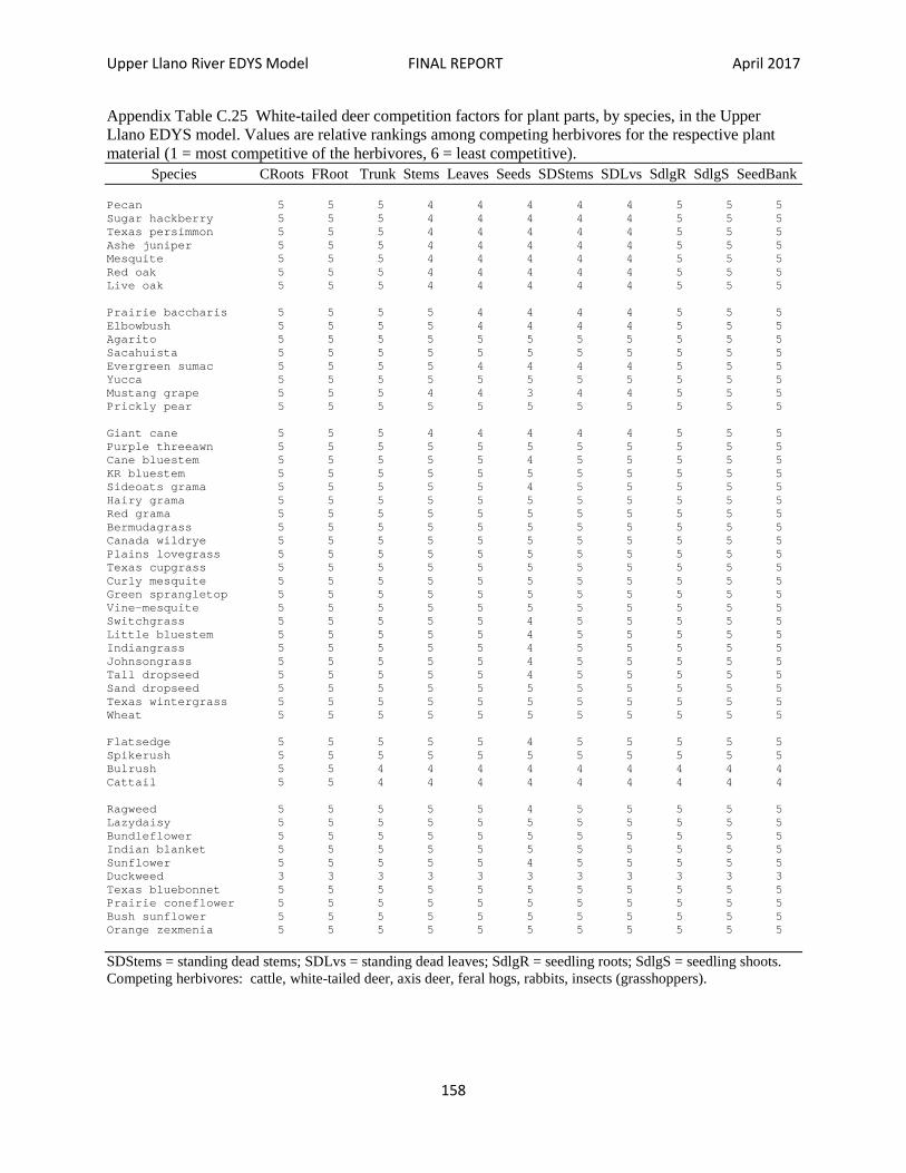
Upper Llano River EDYS Model FINAL REPORT April 2017
158
Appendix Table C.25 White-tailed deer competition factors for plant parts, by species, in the Upper Llano EDYS model. Values are relative rankings among competing herbivores for the respective plant material (1 = most competitive of the herbivores, 6 = least competitive). Species CRoots FRoot Trunk Stems Leaves Seeds SDStems SDLvs SdlgR SdlgS SeedBank Pecan 5 5 5 4 4 4 4 4 5 5 5 Sugar hackberry 5 5 5 4 4 4 4 4 5 5 5 Texas persimmon 5 5 5 4 4 4 4 4 5 5 5 Ashe juniper 5 5 5 4 4 4 4 4 5 5 5 Mesquite 5 5 5 4 4 4 4 4 5 5 5 Red oak 5 5 5 4 4 4 4 4 5 5 5 Live oak 5 5 5 4 4 4 4 4 5 5 5 Prairie baccharis 5 5 5 5 4 4 4 4 5 5 5 Elbowbush 5 5 5 5 4 4 4 4 5 5 5 Agarito 5 5 5 5 5 5 5 5 5 5 5 Sacahuista 5 5 5 5 5 5 5 5 5 5 5 Evergreen sumac 5 5 5 5 4 4 4 4 5 5 5 Yucca 5 5 5 5 5 5 5 5 5 5 5 Mustang grape 5 5 5 4 4 3 4 4 5 5 5 Prickly pear 5 5 5 5 5 5 5 5 5 5 5 Giant cane 5 5 5 4 4 4 4 4 5 5 5 Purple threeawn 5 5 5 5 5 5 5 5 5 5 5 Cane bluestem 5 5 5 5 5 4 5 5 5 5 5 KR bluestem 5 5 5 5 5 5 5 5 5 5 5 Sideoats grama 5 5 5 5 5 4 5 5 5 5 5 Hairy grama 5 5 5 5 5 5 5 5 5 5 5 Red grama 5 5 5 5 5 5 5 5 5 5 5 Bermudagrass 5 5 5 5 5 5 5 5 5 5 5 Canada wildrye 5 5 5 5 5 5 5 5 5 5 5 Plains lovegrass 5 5 5 5 5 5 5 5 5 5 5 Texas cupgrass 5 5 5 5 5 5 5 5 5 5 5 Curly mesquite 5 5 5 5 5 5 5 5 5 5 5 Green sprangletop 5 5 5 5 5 5 5 5 5 5 5 Vine-mesquite 5 5 5 5 5 5 5 5 5 5 5 Switchgrass 5 5 5 5 5 4 5 5 5 5 5 Little bluestem 5 5 5 5 5 4 5 5 5 5 5 Indiangrass 5 5 5 5 5 4 5 5 5 5 5 Johnsongrass 5 5 5 5 5 4 5 5 5 5 5 Tall dropseed 5 5 5 5 5 4 5 5 5 5 5 Sand dropseed 5 5 5 5 5 5 5 5 5 5 5 Texas wintergrass 5 5 5 5 5 5 5 5 5 5 5 Wheat 5 5 5 5 5 5 5 5 5 5 5 Flatsedge 5 5 5 5 5 4 5 5 5 5 5 Spikerush 5 5 5 5 5 5 5 5 5 5 5 Bulrush 5 5 4 4 4 4 4 4 4 4 4 Cattail 5 5 4 4 4 4 4 4 4 4 4 Ragweed 5 5 5 5 5 4 5 5 5 5 5 Lazydaisy 5 5 5 5 5 5 5 5 5 5 5 Bundleflower 5 5 5 5 5 5 5 5 5 5 5 Indian blanket 5 5 5 5 5 5 5 5 5 5 5 Sunflower 5 5 5 5 5 4 5 5 5 5 5 Duckweed 3 3 3 3 3 3 3 3 3 3 3 Texas bluebonnet 5 5 5 5 5 5 5 5 5 5 5 Prairie coneflower 5 5 5 5 5 5 5 5 5 5 5 Bush sunflower 5 5 5 5 5 5 5 5 5 5 5 Orange zexmenia 5 5 5 5 5 5 5 5 5 5 5
SDStems = standing dead stems; SDLvs = standing dead leaves; SdlgR = seedling roots; SdlgS = seedling shoots. Competing herbivores: cattle, white-tailed deer, axis deer, feral hogs, rabbits, insects (grasshoppers).

Upper Llano River EDYS Model FINAL REPORT April 2017
159
Appendix Table C.26 Accessability of plant parts, by species, for consumption by white-tailed deer in the Upper Llano EDYS model. Values are percentages of standing crop biomass of mature plants that could be accessed by white-tailed deer. Species CRoot FRoot Trunk Stems Leaves Seeds SDStem SDLvs SdlgR SdlgS SeedBank Pecan 00 00 01 05 04 01 05 04 00 95 05 Sugar hackberry 00 00 01 05 04 01 05 04 20 90 01 Texas persimmon 00 00 05 20 20 10 20 20 20 95 02 Ashe juniper 00 00 05 25 30 20 25 30 10 90 01 Mesquite 00 00 02 20 20 10 20 20 05 75 05 Red oak 00 00 01 10 10 05 10 10 05 90 05 Live oak 00 00 01 15 15 05 15 15 05 90 05 Prairie baccharis 00 00 10 50 50 05 50 50 05 75 00 Elbowbush 00 00 25 90 90 50 90 90 05 75 01 Agarito 00 00 50 95 95 90 95 95 05 50 01 Sacahuista 00 00 90 95 95 90 95 95 05 50 00 Evergreen sumac 00 00 10 50 50 50 50 50 05 90 00 Yucca 00 00 90 95 95 95 95 95 10 80 01 Mustang grape 00 00 20 05 05 05 05 05 05 90 00 Prickly pear 01 00 90 95 95 95 95 95 10 80 00 Giant cane 01 01 50 70 80 01 70 80 01 90 00 Purple threeawn 00 00 80 90 90 90 90 90 10 50 00 Cane bluestem 00 00 80 90 90 90 90 90 10 70 00 KR bluestem 01 00 80 80 80 90 80 80 10 60 00 Sideoats grama 01 00 80 90 90 90 90 90 10 70 00 Hairy grama 00 00 70 90 90 90 90 90 05 30 00 Red grama 00 00 70 90 90 90 90 90 05 25 00 Bermudagrass 01 00 50 80 80 90 80 80 05 25 00 Canada wildrye 00 00 80 90 90 90 90 90 10 70 01 Plains lovegrass 00 00 80 90 90 90 90 90 10 60 00 Texas cupgrass 00 00 80 90 90 90 90 90 10 70 00 Curly mesquite 00 00 50 80 80 90 80 80 05 30 00 Green sprangletop 00 00 70 90 90 90 90 90 10 60 00 Vine-mesquite 01 00 60 80 80 90 80 80 05 60 00 Switchgrass 00 00 70 90 90 80 90 90 10 70 00 Little bluestem 00 00 80 90 90 90 90 90 10 70 00 Indiangrass 00 00 80 90 90 90 90 90 10 70 01 Johnsongrass 01 00 80 90 90 90 90 90 10 70 01 Tall dropseed 00 00 80 90 90 90 90 90 05 60 00 Sand dropseed 00 00 80 90 90 90 90 90 05 50 00 Texas wintergrass 00 00 70 90 90 80 90 90 05 40 00 Wheat 02 01 90 95 95 95 95 95 10 90 50 Flatsedge 00 00 80 80 80 90 80 80 10 60 00 Spikerush 02 00 50 90 90 90 90 90 05 40 00 Bulrush 05 05 50 70 80 50 70 80 10 50 00 Cattail 10 05 50 80 90 50 80 90 10 60 00 Ragweed 00 00 90 90 90 90 90 90 05 25 00 Lazydaisy 00 00 90 90 90 95 90 90 05 25 00 Bundleflower 00 00 80 90 90 90 90 90 05 25 00 Indian blanket 00 00 70 90 90 95 90 90 05 30 00 Sunflower 00 00 90 95 95 90 95 95 10 50 01 Duckweed 10 10 90 80 80 80 80 80 25 50 00 Texas bluebonnet 00 00 70 90 90 95 90 90 05 25 05 Prairie coneflower 00 00 70 90 90 95 90 90 05 25 00 Bush sunflower 00 00 80 90 90 95 90 90 05 30 00 Orange zexmenia 00 00 80 90 90 90 90 90 05 30 00
SDStem = standing dead stems; SDLvs = standing dead leaves; SdlgR = seedling roots; SdlgS = seedling shoots.

Upper Llano River EDYS Model FINAL REPORT April 2017
160
APPENDIX D ANIMAL DATA Appendix Table D.1 Estimation of cattle stocking rates (moderate level) for vegetation plot types in the three spatial domains (Edwards-Real, Kimble, Sutton) of the Upper Llano EDYS model. Values assume fair range condition and no woody plant cover. Range Type Soil Annual Forage Available AU Forage Requirement Stocking Rate Type (g/m2) Forage (g/m2) (g/AUD)(365 d) (m2/AU) (ac/AU)
Edwards-Real Clay flat IrA 110 55 5,151,975 93,690 20.67 Clay loam RdB 225 112 5,151,975 45,998 11.36 Deep redland LkB 267 133 5,151,975 38,737 9.57 Draw DeB 130 65 5,151,975 79,261 19.58 Gravelly redland DnD 270 135 5,151,975 38,155 9.43 Limestone hill ErB 115 57 5,151,975 90,386 22.33 Loamy bottomland OdA 375 187 5,151,975 27,551 6.81 Low stony hill EcF 197 98 5,151,975 52,571 12.99 Shallow PTD 188 94 5,151,975 44,170 10.91 Steep rocky EcF 197 98 5,151,975 52,571 12.99 Very shallow PeB 155 77 5,151,975 66,909 16.53 Mean 13.93
Kimble Clay flat TsA 245 122 5,151,975 42,229 10.43 Clay loam NuB 214 107 5,151,975 48,149 11.89 Draw De 260 130 5,151,975 39,631 9.79 Loamy bottomland Fr 290 145 5,151,975 35,531 8.78 Low stony hill TaC 129 64 5,151,975 80,500 19.89 Red sandy loam OhC 120 60 5,151,975 85,866 21.21 Sandy loam MnB 192 96 5,151,975 53,666 13.26 Shallow KTB 131 65 5,151,975 79,261 19.58 Steep adobe RbF 100 50 5,151,975 103,040 25.45 Steep rocky TrG 132 66 5,151,975 78,060 19.28 Very shallow CoC 100 50 5,151,975 103,040 25.45 Mean 16.82
Sutton Clay flat Tc 245 122 5,151,975 42,229 10.43 Clay loam Ky 235 117 5,151,975 44,035 10.88 Draw 3 200 100 5,151,975 51,520 12.73 Limestone hill Es 172 86 5,151,975 59,907 14.80 Loamy Rc 235 117 5,151,975 44,035 10.88 Loamy bottomland FD 290 145 5,151,975 35,531 8.78 Low stony hill Ts 172 86 5,151,975 59,907 14.80 Shallow Kt 173 86 5,151,975 59,907 14.80 Steep rocky Tr 172 86 5,151,975 59,907 14.80 Very shallow 2 160 80 5,151,975 64,400 15.91 Mean 12.88
Soil types are listed in Table 5.1 and range types in Table 6.6. Annual Forage = fair range condition (Appendix Tables B.1-B.3). Available Forage = (Annual forage)(0.5), where 0.5 is proper management harvest rate. AU Forage Requirement = 14,115 g/AUD (Tables 7.1 and 7.2). Stocking Rate = (AU Forage Requirement)/(Available Forage)

Upper Llano River EDYS Model FINAL REPORT April 2017
161
Appendix Table D.2 Estimated cattle stocking rates accounting for woody plant cover (average woody plant cover per EDYS type) in the three spatial domains of the Upper Llano EDYS model. Moderate stocking and fair range condition are assumed. Range Type Woody Cover Available Forage Stocking Rate (%) (g/m2) (m2/AU) (ac/AU) Edwards-Real Clay flat 0 55 93,690 20.67 Clay flat 5 53 97,207 24.01 Clay flat 18 47 109,616 27.08 Clay flat 83 18 286,221 70.71 Clay loam 5 108 47,703 11.78 Clay loam 18 96 53,666 13.26 Clay loam 38 78 66,051 16.32 Clay loam 63 56 92,000 22.73 Clay loam 83 37 139,243 34.40 Clay loam 95 27 190,814 47.14 Deep redland 5 128 40,250 9.97 Deep redland 18 115 44,800 11.07 Deep redland 38 93 55,398 13.68 Deep redland 63 66 78,060 19.28 Draw 5 62 83,096 20.53 Draw 18 56 92,000 22.73 Draw 38 46 112,000 27.67 Draw 63 32 160,999 39.77 Draw 83 22 234,181 57.85 Draw 95 16 321,998 79.54 Gravelly redland 5 130 39,631 9.81 Gravelly redland 18 117 44,034 10.88 Gravelly redland 38 95 54,231 13.40 Gravelly redland 63 67 76,895 19.00 Gravelly redland 83 45 114,488 28.28 Limestone hill 5 55 93,672 23.14 Limestone hill 18 49 105,142 25.97 Limestone hill 38 40 128,799 31.82 Limestone hill 63 28 183,999 45.45 Limestone hill 83 19 271,157 66.98 Loamy bottomland 5 180 28,622 7.07 Loamy bottomland 18 161 32,000 7.91 Loamy bottomland 38 141 36,539 9.03 Loamy bottomland 63 93 55,398 13.68 Loamy bottomland 83 62 83,096 20.53 Loamy bottomland 95 45 114,488 28.28 Low stony hill 5 94 54,808 13.54 Low stony hill 18 84 61,333 15.15 Low stony hill 38 69 74,666 18.45 Low stony hill 63 49 105,142 25.97 Low stony hill 83 33 156,120 38.57 Low stony hill 95 24 214,666 53.03 Shallow 5 90 57,244 14.14 Shallow 18 81 63,605 15.71 Shallow 38 66 78,060 19.28 Shallow 63 47 109,616 27.08 Shallow 83 31 166,193 41.06 Shallow 95 23 223,999 55.34 Steep rocky 5 94 54,808 13.54 Steep rocky 18 84 61,333 15.15 Steep rocky 38 69 74,666 18.45 Steep rocky 63 49 105,142 25.97 Steep rocky 83 33 156,120 38.57 Steep rocky 95 24 214,666 53.03 Very shallow 5 74 69,621 17.20 Very shallow 18 66 78,060 19.28 Very shallow 38 54 95,407 23.57 Very shallow 63 38 135,578 33.49 Very shallow 83 26 198,153 48.95 Very shallow 95 18 286,221 70.71

Upper Llano River EDYS Model FINAL REPORT April 2017
162
Appendix Table D.2 (cont.) Range Type Woody Cover Available Forage Stocking Rate (%) (g/m2) (m2/AU) (ac/AU)
Kimble Clay flat 5 117 44,034 10.88 Clay flat 38 86 59,907 14.80 Clay loam 5 103 50,019 12.36 Clay loam 18 92 56,000 13.83 Clay loam 38 75 68,693 16.97 Clay loam 63 53 97,207 24.01 Clay loam 83 36 143,110 35.35 Clay loam 95 26 198,153 48.95 Draw 5 125 41,216 10.18 Draw 18 112 46,000 11.36 Draw 38 91 56,615 13.99 Draw 63 65 79,261 19.58 Draw 83 43 119,813 29.60 Draw 95 31 166,193 41.06 Loamy bottomland 5 139 37,065 9.16 Loamy bottomland 18 125 41,216 10.18 Loamy bottomland 38 102 50,117 12.38 Loamy bottomland 63 72 71,555 17.68 Loamy bottomland 83 48 107,333 26.52 Loamy bottomland 95 35 147,199 36.36 Low stony hill 5 61 84,459 20.86 Low stony hill 18 55 93,672 23.14 Low stony hill 38 45 114,488 28.28 Low stony hill 63 32 160,999 39.77 Low stony hill 83 21 245,332 60.61 Low stony hill 95 15 343,465 84.85 Red sandy loam 18 50 103,039 25.45 Red sandy loam 63 30 171,732 42.42 Sandy loam 38 67 76,895 19.00 Sandy loam 63 48 107,333 26.52 Shallow 0 65 79,261 19.58 Shallow 5 62 83,096 20.53 Shallow 18 56 92,000 22.73 Shallow 38 46 112,000 27.67 Shallow 63 32 160,999 39.77 Shallow 83 22 234,181 57.85 Shallow 95 16 321,998 79.54 Steep adobe 5 48 107,333 26.52 Steep adobe 18 43 119,813 29.60 Steep adobe 38 35 147,199 36.36 Steep adobe 63 25 206,079 50.91 Steep adobe 83 17 303,057 74.87 Steep adobe 95 12 429,248 106.04 Steep rocky 5 63 81,777 20.20 Steep rocky 18 57 90,386 22.33 Steep rocky 38 46 111,999 27.67 Steep rocky 63 33 156,120 38.57 Steep rocky 83 22 234,181 57.85 Steep rocky 95 16 321,998 79.54 Very shallow 5 48 107,333 26.52 Very shallow 18 43 119,813 29.60 Very shallow 38 35 147,199 36.36 Very shallow 63 25 206,079 50.91
Sutton Clay flat 0 122 42,229 10.43 Clay flat 5 117 44,034 10.88 Clay flat 18 105 49,066 12.12 Clay flat 38 85 60,611 14.97 Clay flat 63 61 84,459 20.86 Clay flat 83 41 125,658 31.04

Upper Llano River EDYS Model FINAL REPORT April 2017
163
Appendix Table D.2 (cont.) Range Type Woody Cover Available Forage Stocking Rate (%) (g/m2) (m2/AU) (ac/AU) Clay loam 5 112 46,000 11.36 Clay loam 18 101 51,010 12.60 Clay loam 38 82 62,829 15.52 Clay loam 63 58 88,827 21.94 Clay loam 83 39 132,102 32.61 Clay loam 95 28 183,999 45.45 Draw 5 96 53,666 13.26 Draw 38 70 73,600 18.18 Draw 63 50 103,039 25.45 Limestone hill 5 83 62,072 15.33 Limestone hill 83 29 177,654 43.89 Loamy 38 82 62,829 15.52 Loamy bottomland 5 139 37,065 9.16 Loamy bottomland 18 125 41,216 10.18 Loamy bottomland 38 102 50,117 12.38 Loamy bottomland 63 72 71,555 17.68 Loamy bottomland 83 48 107,333 26.52 Low stony hill 5 83 62,072 15.33 Low stony hill 18 74 69,621 17.20 Low stony hill 38 60 85,866 21.21 Low stony hill 63 43 119,813 29.60 Low stony hill 83 29 177,654 43.89 Low stony hill 95 21 245,332 60.61 Shallow 5 83 62,072 15.33 Shallow 18 74 69,621 17.20 Shallow 38 60 85,866 21.21 Shallow 63 43 119,813 29.60 Shallow 83 29 177,654 43.89 Shallow 95 21 245,332 60.61 Steep rocky 5 83 62,072 15.33 Steep rocky 18 74 69,621 17.20 Steep rocky 38 60 85,866 21.21 Steep rocky 63 43 119,813 29.60 Steep rocky 83 29 177,654 43.89 Very shallow 5 77 66,909 16.53 Very shallow 18 69 74,666 18.45 Very shallow 38 56 92,000 22.73 Very shallow 63 40 128,799 31.82
Available forage adjusted for woody plant cover = (amount at 0% woody cover)[1.00 – (0.8)woody plant cover)]. Forage requirement = 14,115 g/AUD (Tables 7.1 and 7.2). Stocking rate = (forage requirement)(365 days)/(available forage).

Upper Llano River EDYS Model FINAL REPORT April 2017
164
Appendix Table D.3 Estimated cattle stocking rates on disturbed sites, accounting for woody plant cover, in the three spatial domains of the Upper Llano EDYS model. Moderate stocking is assumed. Disturbance Woody Cover Available Forage Stocking Rate Type (%) (g/m2) (m2/AU) (ac/AU) Edwards-Real Brush controlled 5 10 515,198 127.27 Brush controlled 18 96 53,666 13.26 Brush controlled 38 78 66,051 16.32 Pit 5 28 183,999 45.45
Kimble Brush controlled 5 10 515,198 127.27 Brush controlled 18 92 56,000 13.83 Brush controlled 38 75 68,693 16.97 Brush controlled 63 53 97,207 24.01
Sutton Brush controlled 0 10 515,198 127.27 Brush controlled 5 10 515,198 127.27 Brush controlled 18 101 51,010 12.60 Brush controlled 38 82 62,829 15.52 Brush controlled 63 58 88,827 21.94 Brush controlled 83 39 132,102 32.61 Pits caliche 18 28 183,999 45.45
Available forage for 0 and 5% brush controlled and pits = 0.5(grass biomass value from Appendix Table B.11). Available forage for 18-83 brush controlled = available forage value for clay loam sites (Appendix Table D.2) at respective woody plant coverage and spatial domain. Forage requirement = 14,115 g/AUD (Tables 7.1 and 7.2). Stocking rate = (forage requirement)(365 days)/(available forage).