development of pilot high-resolution gridded poverty ... · pdf filedevelopment of...

Development of High-Resolution Gridded Poverty Surfaces

Development of Pilot High-Resolution Gridded Poverty Surfaces: Methods

working paper

Dr Andrew Tatem Dr Peter Gething Dr Carla Pezzulo

Dr Dan Weiss Dr Samir Bhatt


1.0 OVERVIEW

Improved understanding of geographic variation and inequity in health status, wealth, and access to resources within countries is increasingly recognized as central to meeting development goals. Development indicators assessed at national scales can often conceal important inequities, with the rural poor often least well represented. As international funding for development comes under pressure, the ability to target limited resources to underserved groups becomes crucial. Monitoring inequalities for targeting interventions requires a reliable and detailed evidence base. While high-resolution spatial data on population distributions in resource poor areas are now becoming available (e.g. www.worldpop.org.uk), comprehensive information on demographic, health and wealth attributes of those populations remain only usable at highly aggregated regional levels through national household surveys (e.g. www.measuredhs.com). The Demographic and Health Survey (DHS) program has been a leader in collecting and providing cluster-randomised survey data on core development indicators. In addition to their standard open-source data files in which survey results are tabulated by first-order sub-national regions (for example at province or state level) and urban/rural strata, more recent surveys now provide geocoded data for individual clusters. The availability of the GPS coordinates for DHS clusters provides, for the first time, highly resolved locational information that can be linked with survey outputs for quantifying demographic and health status heterogeneities and inequities. Here we present a novel spatial statistical methodology for the production of gridded surfaces of household survey-based variables, focusing on poverty mapping. A Bayesian geostatistical modeling framework, following approaches constructed for the Malaria Atlas Project, has been established to exploit spatiotemporal relationships within the data, leverage ancillary information from an extensive set of covariates, and rigorously handle uncertainties at all stages to generate robust output surfaces with accompanying confidence intervals.

2.0 ASSEMBLING CANDIDATE GEOSPATIAL COVARIATES OF POVERTY

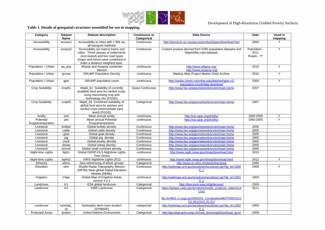
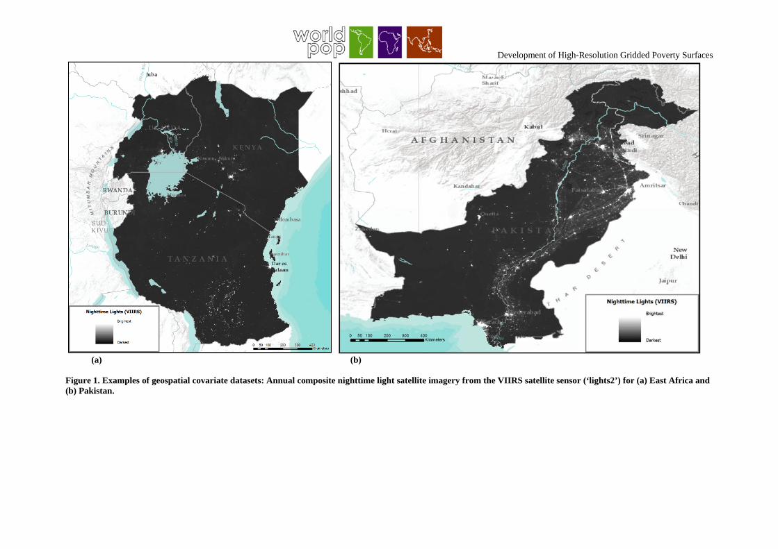
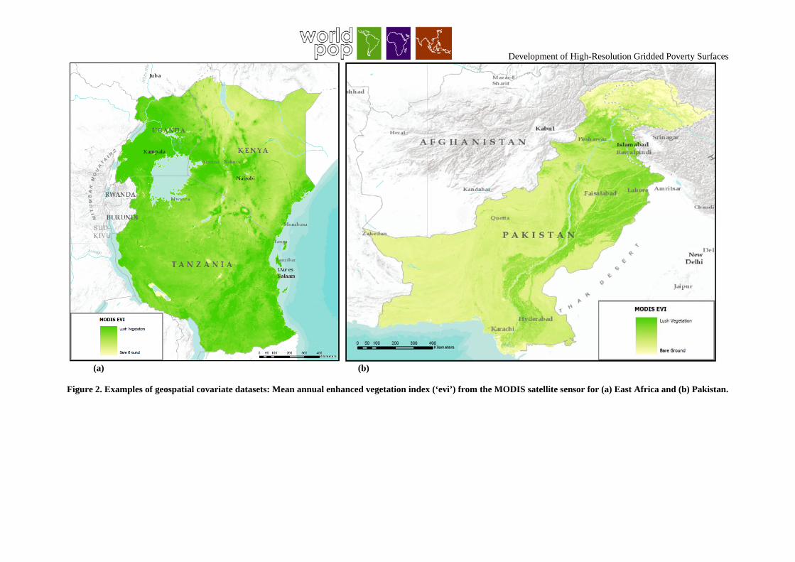
A suite of geospatial covariates were assembled for use in the mapping, focussing on factors likely to have an impact on determining levels of poverty. Table 1 provides details on each of the geospatial covariate datasets. The datasets are all provided at differing formats, spatial resolutions, projections and extents. Thus, algorithms were constructed and applied to convert polygon files to gridded datasets and then regrid each gridded dataset to a common 1km spatial resolution grid-frame for use in map production. Figures 1 and 2 show examples of two of the datasets described in table 1 (lights2 and evi). While a large suite of data was compiled, not all of the datasets in table 1 were included in the mapping due to differing levels of reliability, relevance and variations in data formats. Many datasets were ultimately left out due to poor spatial resolution and/or categorical inputs that were tested and didn't add sufficient extra information to improve model accuracies.


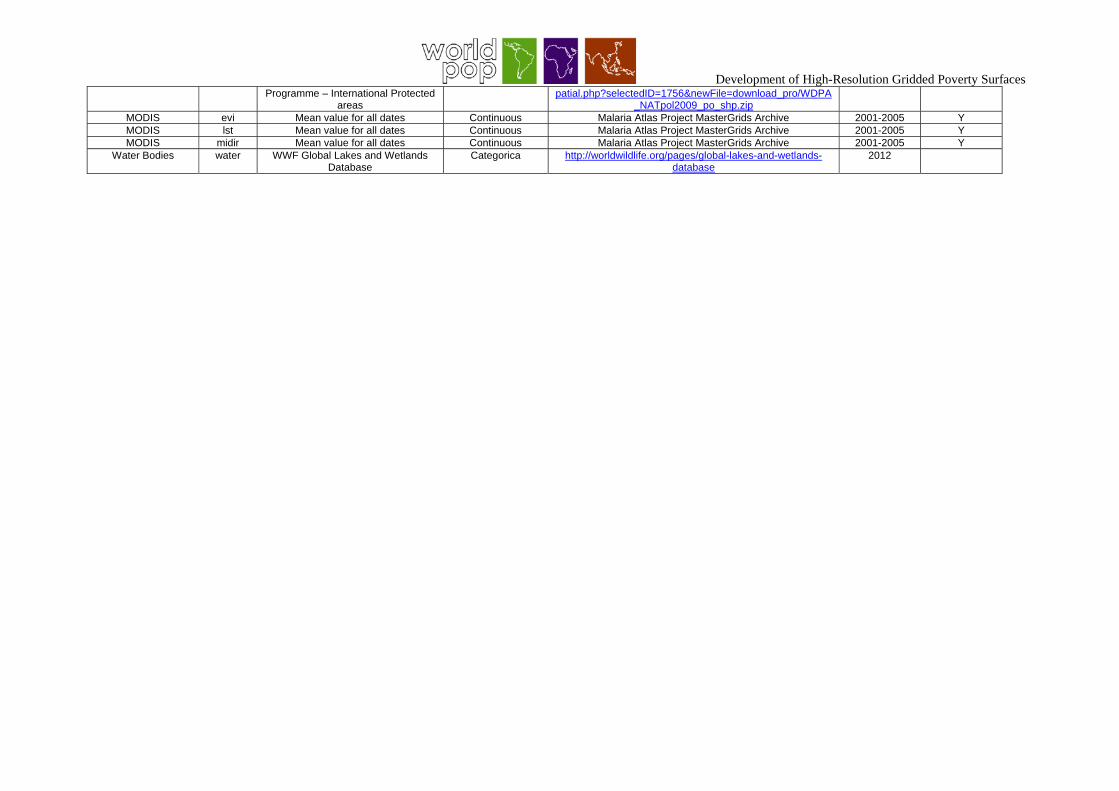
Table 1. Details of geospatial covariates assembled for use in mapping.

Category Dataset Name

Dataset description Continuous or Categorical

Data Source Date Used in mapping

Accessibility access1 Accessibility to cities with > 50k via all transport methods

Continuous http://bioval.jrc.ec.europa.eu/products/gam/download.htm 2000

Y

Accessibility access2 Accessibility via road to towns and cities. Three classes of settlements

(size based) and two road types (major and minor) were combined to

make a distance weighted layer.

Continuous Custom product derived from ESRI population datasets and MapAbility road datasets

Population -2011

Roads - ??

Y

Population / Urban aa_pop Afripop and Asiapop combined dataset

continuous http://www.afripop.org/ http://www.asiapop.org/

2010 Y

Population / Urban grump GRUMP Population Density continuous Malaria Atlas Project Master Grids Archive 2010

Y

Population / Urban gpw GRUMP population count continuous http://sedac.ciesin.columbia.edu/data/set/gpw-v3-population-count/data-download

2000 Y

Crop Suitability crop61 Map6_61 Suitability of currently available land area for rainfed crops,

using maximising crop and technology mix (FGGD)

Quasi Continuous http://www.fao.org/geonetwork/srv/en/main.home 2007

Crop Suitability crop63 Map6_63 Combined suitability of global land area for pasture and rainfed crops (intermediate input

level) (FGGD)

Categorical http://www.fao.org/geonetwork/srv/en/main.home 2007

Aridity arid Mean annual aridity continuous http://csi.cgiar.org/Aridity/ 1950-2000 Y Potential

Evapotranspiration pet Mean annual Potential

Evapotranspiration continuous http://csi.cgiar.org/Aridity/ 1950-2000 Y

Livestock buffalo Global buffalo density Continuous http://www.fao.org/geonetwork/srv/en/main.home 2005 Livestock cattle Global cattle density Continuous http://www.fao.org/geonetwork/srv/en/main.home 2005 Livestock goat Global goat density Continuous http://www.fao.org/geonetwork/srv/en/main.home 2005 Livestock pig Global pig density Continuous http://www.fao.org/geonetwork/srv/en/main.home 2005 Livestock poult Global poultry density Continuous http://www.fao.org/geonetwork/srv/en/main.home 2005 Livestock sheep Global sheep density Continuous http://www.fao.org/geonetwork/srv/en/main.home 2005 Livestock smrum Global small ruminant density Continuous http://www.fao.org/geonetwork/srv/en/main.home 2005

Night-time Lights light1 Global DMSP-OLS Nighttime Lights Time Series

continuous http://www.ngdc.noaa.gov/dmsp/download.html 2010

Night-time Lights lights2 VIIRS Nighttime Lights-2012 continuous http://www.ngdc.noaa.gov/dmsp/download.html 2012 Y Ethnicity ethnic Geo-referencing of ethnic groups Categorical http://www.icr.ethz.ch/data/other/greg 1994 Elevation elev Shuttle Radar Topography Mission

(SRTM) Near-global Digital Elevation Models (DEMs)

Continuous http://webmap.ornl.gov/wcsdown/wcsdown.jsp?dg_id=10008_1

2000 Y

Irrigation irriga Global Map of Irrigation Areas version 4.0.1

continuous http://webmap.ornl.gov/wcsdown/wcsdown.jsp?dg_id=10013_1

2000

Landcover lc1 ESA global landcover Categorical http://due.esrin.esa.int/globcover/ 2009 Landcover lc2 IGBP Landcover Categorical https://lpdaac.usgs.gov/products/modis_products_table/mcd

12q1

ftp://e4ftl01.cr.usgs.gov/MODIS_Composites/MOTA/MCD12Q1.051/2011.01.01/

2011

Landcover synmap_1k

Synergetic land cover product (SYNMAP)

categorical http://webmap.ornl.gov/wcsdown/wcsdown.jsp?dg_id=10024_1

2000

Protected Areas protect United Nations Environment Categorical http://geodata.grid.unep.ch/mod_download/download_geos 2009


Programme – International Protected areas

patial.php?selectedID=1756&newFile=download_pro/WDPA_NATpol2009_po_shp.zip

MODIS evi Mean value for all dates Continuous Malaria Atlas Project MasterGrids Archive 2001-2005 Y MODIS lst Mean value for all dates Continuous Malaria Atlas Project MasterGrids Archive 2001-2005 Y MODIS midir Mean value for all dates Continuous Malaria Atlas Project MasterGrids Archive 2001-2005 Y

Water Bodies water WWF Global Lakes and Wetlands Database

Categorica http://worldwildlife.org/pages/global-lakes-and-wetlands-database

2012


(a) (b)

Figure 1. Examples of geospatial covariate datasets: Annual composite nighttime light satellite imagery from the VIIRS satellite sensor (‘lights2’) for (a) East Africa and (b) Pakistan.


(a) (b)

Figure 2. Examples of geospatial covariate datasets: Mean annual enhanced vegetation index (‘evi’) from the MODIS satellite sensor for (a) East Africa and (b) Pakistan.


3.0 CREATION OF PILOT POVERTY MAPS

Using either the Multidimensional Poverty Index (MPI) or consumption-based <$1.25/$2 a day headcounts as our test variable, we implemented a model-based geostatistical framework to generate pilot poverty maps at 1x1km resolution. Here we describe the exploratory analysis and model formulation.

3.1 METHODS

3.1.1 Model structure Our initial model structure is a class of generalized linear mixed model, with an approximation of a multivariate Normal random field (i.e. a Gaussian Process) used as a spatially autocorrelated random effect term. This family of models derives from a body of theory knows as model-based geostatistics. The poverty headcount ratio (proportion of individuals considered ‘poor’ according to the MPI

or consumption-based index – in the example notation, MPI is used here) iMPIh x , at each

location was modeled as a transformation of a spatially structured field superimposed with additional random variation . The count of individuals considered poor from the total sample of in each survey cluster was modeled as a conditionally independent binomial variate

given the unobserved underlying iMPIh x value. The spatial component was represented by a

stationary Gaussian process with mean and covariance . The unstructured component was represented as Gaussian with zero mean and variance . Both the inference and

prediction stages were coded using the INLA framework, primarily in R.

3.1.1.1 Mean and covariance definition

The mean component was modelled as a linear function of n=12 environmental covariates,

,where was a vector consisting of a constant and the covariates indexed by spatial location , and was a corresponding vector of regression coefficients. Each covariate was converted to z-scores before analysis. In this pilot stage, we took an inclusive approach to covariate selection, with most of the assembled variables being included in the model. As our library of covariates becomes more refined, we will implement more formal model selection procedures to identify optimal covariate suites for inclusion. Covariance between spatial locations was modeled using a Matern covariance function :

2

1

( ; ) ( ; )1( ; ) 2 2

2i j i j

i j

d x x d x xC d x x K


Where ( ; )i jd x x is the geographical separation between two points; , , are parameters of the

covariance function defining, respectively, its amplitude, degree of differentiability, and scale; K is the modified Bessel function of the second kind of order , and is the gamma function.

3.1.2 Model implementation and output

Bayesian inference was implemented using the INLA algorithm to generate approximations of

the marginal posterior distributions of the outcome variable iMPIh x at each location on a

regular 1 × 1 km spatial grid across the country of interest and of the unobserved parameters of the mean, covariance function and Gaussian random noise component. At each location, the posterior distribution was summarized using the posterior mean as a point estimate, and the posterior inter-quartile range as a measure of model precision. Maps were generated of each of these metrics in ArcGIS 10.2.

3.1.3 Validation

The predictive performance of each model was assessed via out-of-sample validation. We implemented a ten-fold hold-out procedure whereby 10% of the data points were randomly withdrawn from the dataset, the model run in full using the remaining 90% of data, and the predicted values at the locations of the hold-out data compared to their observed values. This was repeated ten times without replacement such that every data point was held out once across the ten validation runs. Standard validation statistics were computed as measures of model precision (root mean square error, mean absolute error), bias (mean error), and correlation between observed and predicted. We also generated a scatter plot of observed versus predicted values. Outputs for each country are available upon request and will be published in an extended manuscript.


4.0 ACKNOWLEDGEMENTS

We are grateful to the following people for their advice and input: Karina Nielsen and Jake Kendall at the Bill and Melinda Gates Foundation, Clara Burgert and her team at Measure DHS, Peter Lanjouw and his team at the World Bank, Catherine Linard, Andrea Gaughan and Forrest Stevens at WorldPop.

development of pilot high-resolution gridded poverty ... · pdf filedevelopment of...

Documents