development of techniques for quantum-enhanced laser

Development of Techniques for Quantum-Enhanced

Laser-Interferometric Gravitational-Wave Detectors

by

Keisuke Goda

B.S., University of California at Berkeley (2001)

Submitted to the Department of Physicsin partial fulfillment of the requirements for the degree of

Doctor of Philosophy

at the

MASSACHUSETTS INSTITUTE OF TECHNOLOGY

August 2007

c© Keisuke Goda, MMVII. All rights reserved.

The author hereby grants to MIT permission to reproduce and distribute publiclypaper and electronic copies of this thesis document in whole or in part.

Author . . . . . . . . . . . . . . . . . . . . . . . . . . . . . . . . . . . . . . . . . . . . . . . . . . . . . . . . . . . . . . . . . . . . . . . . . . . .Department of Physics

August 10, 2007

Certified by. . . . . . . . . . . . . . . . . . . . . . . . . . . . . . . . . . . . . . . . . . . . . . . . . . . . . . . . . . . . . . . . . . . . . . . .Nergis Mavalvala

Associate Professor of PhysicsThesis Supervisor

Accepted by . . . . . . . . . . . . . . . . . . . . . . . . . . . . . . . . . . . . . . . . . . . . . . . . . . . . . . . . . . . . . . . . . . . . . . .Thomas J. Greytak

Associate Department Head for Education

Development of Techniques for Quantum-Enhanced

Laser-Interferometric Gravitational-Wave Detectors

by

Keisuke Goda

Submitted to the Department of Physicson August 10, 2007, in partial fulfillment of the

requirements for the degree ofDoctor of Philosophy

Abstract

A detailed theoretical and experimental study of techniques necessary for quantum-enhanced laser-interferometric gravitational wave (GW) detectors was carried out. The basic theory of GWs andlaser-interferometric GW detectors, quantum noise in GW detectors, the theory of squeezed statesincluding generation, degradation, detection, and control of squeezed states using sub-thresholdoptical parametric oscillators (OPOs) and homodyne detectors, experimental characterization ofthese techniques (using periodically poled KTiOPO4 in an OPO at 1064 nm for the first time), keyrequirements for quantum-enhanced GW detectors, and the propagation of a squeezed state in acomplex interferometer and its interaction with the interferometer field were studied. Finally, theexperimental demonstration of quantum-enhancement in a prototype GW detector was performed.By injecting a squeezed vacuum field of 9.3 dB (inferred) or 7.4 ± 0.1 dB (measured) at frequenciesabove 3 kHz and a cutoff frequency for squeezing at 700 Hz into the antisymmetric port of theprototype GW detector in a signal-recycled Michelson interferometer configuration, the shot noisefloor of the detector was reduced broadband from 7.0× 10−17 m/

√Hz to 5.0× 10−17 m/

√Hz while

the strength of a simulated GW signal was retained, resulting in a 40% increase in signal-to-noiseratio or detector sensitivity, which is equivalent to a factor of 1.43 = 2.7 increase in GW detectionrate for isotropically distributed GW sources that are confined to the frequency band in whichsqueezing was effective. This is the first implementation of quantum-enhancement in a prototypeGW detector with suspended optics and readout and control schemes similar to those used in LIGOand Advanced LIGO. It is, therefore, a critical step toward implementation of quantum-enhancementin long baseline GW detectors.

Thesis Supervisor: Nergis MavalvalaTitle: Associate Professor of Physics

Acknowledgments

This thesis has been supported by a number of people. First of all, I would like to thank my

supervisor Nergis Mavalvala for her incredible support. Without a doubt, the 40m squeezing project

would not have been made possible without her constant support. Her leadership, intellectual talent

and curiosity, and unlimited efforts about education for her students including myself have greatly

influenced and inspired me. I admire these aspects of hers and have learned many things from them.

It is not an overstatement that she is one of the greatest mentors at MIT. I am sure her other

students agree on this.

I have had the biggest fortune to work with many talented and inspiring people. First, I must

mention the name of the greatest Russian, Eugeniy E. Mikhailov at the College of William & Mary.

His superb technical skills and expertise about building experimental apparatus impressed me greatly

during his three years at MIT. The 40m squeezing experiment could not have been realized without

the squeezing-related techniques we acquired at MIT. His friendship has been invaluable. I have to

say that I very much enjoyed dining at good restaurants in and near Pasadena almost every night

while he visited Caltech.

Osamu Miyakawa at Caltech has been an incredible supporter as well. Although they were

tough, I enjoyed midnight squeezing experiments with him. He is very good at explaining things

and making difficult concepts easy to understand, which helped me a lot with understanding the

40m interferometer. Among few Japanese people in LIGO, he is a unique scientist with talent in

many aspects and it was the most fun to work with him. Without a doubt, he is a Japanese role

model.

I would like to thank my research collaborators. First, I am grateful to Shailendhar Saraf at

Rochester Institute of Technology for helping me with building important circuits for the squeezing

experiment such as the quantum noise-locking servo with higher stability. I also thank my Australian

collaborators, Kirk McKenzie, Warwick Bowen (currently at University of Otago), Ping Koy Lam,

David McClelland, and Malcolm Gray at Australian National University. Squeezing started in the

LIGO Quantum Measurement Group thanks to these people who told me how to squeeze during my

four-week visit at the university. I would also like to thank the Caltech 40m team, Bob Taylor and

Steve Vass, for clean room work and 40m maintenance, and in particular, Alan Weinstein for his

patient support for the 40m squeezing project. His good nature has maintained the 40m lab healthy

and humorous.

I also thank my colleagues in the Quantum Measurement Group at MIT, Thomas Corbitt,

Christopher Wipf, David Ottaway, and Edith Innerhofer. I am grateful to Chris for helping me with

low-noise photodetector development for the 40m squeezing project, Dave for supervising me on the

wavefront sensor experiment and squeezing work at MIT, and Thomas for stimulating discussion

about squeezing. I remember my old days when Thomas, Chris, and I had to go through the painful

General Exams at MIT.

I would also like to send my gratitude to other LIGO staff members at MIT, Keith Bayer for

his support about computer software and hardware and Ken Mason, for purchasing machined parts.

The squeezing project was based on their help. One of the greatest assistants is LIGO’s secretary,

Marie Woods. Her secretary work is more than excellent in that she does things on time without a

mistake. This was extremely important to do long distance work between MIT and Caltech for the

past two years. I am thankful to David Shoemaker and Scott A. Hughes for their support as thesis

committee members. Their constructive criticism assisted me with writing my thesis better.

I would also like to thank my collaborators on the research outside of the 40m squeezing project.

Kentaro Somiya at Albert Einstein Institute and Yanbei Chen at Caltech are impressive people and

also fun to work with on displacement-noise-free interferometers. I am also grateful for Kentaro’s

help on understanding squeezing in the two-photon picture. I also thank my personal research

collaborators in the MIT Spectroscopy Lab, Gabriel Popescu (currently at University of Illinois at

Urbana-Champaign), Ramachandra R. Dasari, and Michael Feld, and Takahiro Ikeda (currently at

Hamamatsu Photonics). I would like to send my special thanks to Takahiro for showing me the

interesting labs and factory of Hamamatsu Photonics and introducing me to the president of the

company, Teruo Hiruma. I personally admire Hamamatsu’s products since their quality is extremely

important for basic science research. I am also thankful for another personal research collaborator,

Eriko Watanabe, in Kodate Lab at Japan Women’s University. Her strong motivation has always

stimulated me. Seiji Kawamura at National Astronomical Observatory of Japan (NAOJ) kindly

gave me many seminar opportunities at NAOJ.

Outside work hours, there have been numerous people who have helped me. I would like to

thank (in alphabetical order) Akira Okutomi (Nikon), Alexander Patrikalakis (Computer Science,

MIT), Arisa Watanabe, Ayako Komuro, Gautam Kene (Law, Columbia University), Haruka Tanji

(Physics, Harvard University), Hiromi Sato, Kanako Ueno (Institute of Industrial Science, University

of Tokyo), Kanna Watanabe (Massachusetts General Hospital), Kenji Taira (Olympus Corporation),

Kenya Suzuki (NTT Photonics Laboratory), Magnus Hsu (Quantum Optics, Australian National

University), Masaru Tsuchiya (Applied Physics, Harvard University), Misayo Matsumoto (Coach),

Nami Yokofuke, Naoko Kurahashi (Physics, Stanford University), Noriko Shimodaira (XL Soft Cor-

poration), Noriko Yogo (Sun International Group), Paula Popescu (Physics, Harvard University),

Rhea M. Dah-Nomoto (Medical, University of Southern California), Saori Kato, Saori Kitagawa, Tat-

suya Takahashi (Silicon Library Inc.), Tomoko Tada (Neuroscience, MIT), Yasunori Chiaya (Gehry

Partners), Yasushi Takamatsu (Mitsui Chemicals), Yui Ikeshima (L.A. Walker), Yuka Oshimi (L.A.

Shokutsu Club), and my parents Emiko Goda and Masao Goda. I would like to cherish my memory

with my MIT colleagues who have spent a few to several years at MIT as graduate students with

me: Fuwan Gan (Research Lab. of Electronics, MIT), Bo Bai (Goldman Sacks), Ryan Rygg (Plasma

Fusion Center, MIT), Yoshiaki Kuwata (Aeronautics and Astronautics, MIT), Shinya Kurebayashi

(Goldman Sacks), and Fumiaki Toyama (Advanced Micro Devices). I am sure they will be success-

ful anywhere they are. In addition, I have enjoyed 5 years of soccer life at MIT with dozens of

teammates.

Finally, I thank SPIE, Optical Society of America (OSA), and New Focus Inc. for awards and

scholarships. Their financial support helped me with attending conferences and meeting people

for discussion. SPIE and OSA also helped me establish SPIE and OSA student chapters at MIT

to encourage optics research on campus. I acknowledge National Science Foundation’s long-term

financial support for the squeezing research. This work has been supported by the National Science

Foundation Grant Nos. PHY-0107417 and PHY-0300345.

- Keisuke Goda August 8, 2007

Contents

Introduction 21

1 Background 25

1.1 Overview . . . . . . . . . . . . . . . . . . . . . . . . . . . . . . . . . . . . . . . . . . 25

1.2 Gravitational Waves in General Relativity . . . . . . . . . . . . . . . . . . . . . . . . 25

1.2.1 The Nature of Gravitational Waves . . . . . . . . . . . . . . . . . . . . . . . . 25

1.2.2 Gravitational Radiation . . . . . . . . . . . . . . . . . . . . . . . . . . . . . . 27

1.2.3 Astronomical Sources of Gravitational Waves . . . . . . . . . . . . . . . . . . 29

1.3 Laser-Interferometric Gravitational-Wave Detectors . . . . . . . . . . . . . . . . . . . 33

1.3.1 The History of Gravitational-Wave Detectors . . . . . . . . . . . . . . . . . . 33

1.3.2 The Principle of Laser-Interferometric Gravitational-Wave Detectors . . . . . 34

1.4 Quantum Noise in Gravitational-Wave Detectors . . . . . . . . . . . . . . . . . . . . 36

1.4.1 Introduction . . . . . . . . . . . . . . . . . . . . . . . . . . . . . . . . . . . . 36

1.4.2 The Heisenberg Uncertainty Principle . . . . . . . . . . . . . . . . . . . . . . 37

1.4.3 Quantum Noise Sources . . . . . . . . . . . . . . . . . . . . . . . . . . . . . . 39

1.4.4 Quantum Noise in LIGO and Advanced LIGO . . . . . . . . . . . . . . . . . 43

1.4.5 Quantum Limit by Quantum Fluctuations of a Vacuum Field . . . . . . . . . 47

1.5 Quantum-Enhancement . . . . . . . . . . . . . . . . . . . . . . . . . . . . . . . . . . 47

1.5.1 Introduction . . . . . . . . . . . . . . . . . . . . . . . . . . . . . . . . . . . . 47

1.5.2 Ideal Squeezed State Production and Quantum Enhancement . . . . . . . . . 48

1.5.3 Previous Experimental Efforts . . . . . . . . . . . . . . . . . . . . . . . . . . 52

1.6 The Goal of this Work . . . . . . . . . . . . . . . . . . . . . . . . . . . . . . . . . . . 52

2 Theory of Squeezed States 55

2.1 Overview . . . . . . . . . . . . . . . . . . . . . . . . . . . . . . . . . . . . . . . . . . 55

2.2 States of Light . . . . . . . . . . . . . . . . . . . . . . . . . . . . . . . . . . . . . . . 56

2.2.1 The Ball-on-Stick Picture . . . . . . . . . . . . . . . . . . . . . . . . . . . . . 56

2.2.2 Equivalence of Squeezed Light and Squeezed Vacuum . . . . . . . . . . . . . 59

9

2.3 Generation of Squeezed States . . . . . . . . . . . . . . . . . . . . . . . . . . . . . . . 59

2.3.1 Introduction . . . . . . . . . . . . . . . . . . . . . . . . . . . . . . . . . . . . 59

2.3.2 Quantization of Quadrature Field Amplitudes in Two-Photon Formalism . . 60

2.3.3 Generation of Squeezed States in Optical Parametric Oscillation . . . . . . . 63

2.3.4 The Ball-on-Stick Picture Revisited . . . . . . . . . . . . . . . . . . . . . . . 71

2.4 Second-Order Nonlinear Optical Processes for Squeezed State Production . . . . . . 74

2.4.1 Overview . . . . . . . . . . . . . . . . . . . . . . . . . . . . . . . . . . . . . . 74

2.4.2 Atomic Polarization of a Dielectric Medium . . . . . . . . . . . . . . . . . . . 74

2.4.3 Conservation Laws . . . . . . . . . . . . . . . . . . . . . . . . . . . . . . . . . 75

2.4.4 Phase Matching Types . . . . . . . . . . . . . . . . . . . . . . . . . . . . . . . 76

2.4.5 Quasi-Phase-Matching with Periodically Poled Materials . . . . . . . . . . . . 78

2.4.6 Second-Harmonic Generation . . . . . . . . . . . . . . . . . . . . . . . . . . . 83

2.4.7 Classical Optical Parametric Oscillation . . . . . . . . . . . . . . . . . . . . . 86

2.4.8 Designing Stable Resonators with Nonlinear Media . . . . . . . . . . . . . . . 86

2.5 Degradation of Squeezed States . . . . . . . . . . . . . . . . . . . . . . . . . . . . . . 90

2.6 Detection of Squeezed States . . . . . . . . . . . . . . . . . . . . . . . . . . . . . . . 91

2.6.1 Overview . . . . . . . . . . . . . . . . . . . . . . . . . . . . . . . . . . . . . . 91

2.6.2 Balanced Homodyne Detection . . . . . . . . . . . . . . . . . . . . . . . . . . 92

2.6.3 Unbalanced Homodyne Detection . . . . . . . . . . . . . . . . . . . . . . . . . 95

2.7 Control of Squeezed States . . . . . . . . . . . . . . . . . . . . . . . . . . . . . . . . 97

2.7.1 Overview . . . . . . . . . . . . . . . . . . . . . . . . . . . . . . . . . . . . . . 97

2.7.2 Quantum Noise Locking . . . . . . . . . . . . . . . . . . . . . . . . . . . . . . 98

2.7.3 Coherent Control of Squeezing . . . . . . . . . . . . . . . . . . . . . . . . . . 102

3 Experimental Generation, Detection, and Control of Squeezed States 107

3.1 Overview . . . . . . . . . . . . . . . . . . . . . . . . . . . . . . . . . . . . . . . . . . 107

3.2 Experimental Apparatus . . . . . . . . . . . . . . . . . . . . . . . . . . . . . . . . . . 107

3.2.1 Overview . . . . . . . . . . . . . . . . . . . . . . . . . . . . . . . . . . . . . . 107

3.2.2 Laser . . . . . . . . . . . . . . . . . . . . . . . . . . . . . . . . . . . . . . . . 108

3.2.3 Second-Harmonic Generator . . . . . . . . . . . . . . . . . . . . . . . . . . . . 109

3.2.4 Optical Parametric Oscillator . . . . . . . . . . . . . . . . . . . . . . . . . . . 110

3.2.5 Subcarrier Optics . . . . . . . . . . . . . . . . . . . . . . . . . . . . . . . . . . 112

3.2.6 Homodyne Detector . . . . . . . . . . . . . . . . . . . . . . . . . . . . . . . . 114

3.2.7 Quantum Noise Locking . . . . . . . . . . . . . . . . . . . . . . . . . . . . . . 115

3.3 Experimental Results . . . . . . . . . . . . . . . . . . . . . . . . . . . . . . . . . . . . 115

3.3.1 Overview . . . . . . . . . . . . . . . . . . . . . . . . . . . . . . . . . . . . . . 115

3.3.2 Spectrum of Scanned Squeezed Shot Noise . . . . . . . . . . . . . . . . . . . . 116

10

3.3.3 Spectrum of Locked Squeezed Shot Noise . . . . . . . . . . . . . . . . . . . . 118

3.3.4 Verification of Quantum Correlations . . . . . . . . . . . . . . . . . . . . . . . 119

4 Requirements for Quantum Enhanced Gravitational Wave Detectors 121

4.1 Overview . . . . . . . . . . . . . . . . . . . . . . . . . . . . . . . . . . . . . . . . . . 121

4.2 Squeezing in the Gravitational Wave Band . . . . . . . . . . . . . . . . . . . . . . . . 121

4.2.1 Overview . . . . . . . . . . . . . . . . . . . . . . . . . . . . . . . . . . . . . . 121

4.2.2 Seed Noise . . . . . . . . . . . . . . . . . . . . . . . . . . . . . . . . . . . . . 122

4.2.3 Pump Noise . . . . . . . . . . . . . . . . . . . . . . . . . . . . . . . . . . . . . 123

4.2.4 Photothermal Noise . . . . . . . . . . . . . . . . . . . . . . . . . . . . . . . . 123

4.2.5 Scattered Photon Noise . . . . . . . . . . . . . . . . . . . . . . . . . . . . . . 124

4.3 High Level of Squeezing . . . . . . . . . . . . . . . . . . . . . . . . . . . . . . . . . . 124

4.3.1 Overview . . . . . . . . . . . . . . . . . . . . . . . . . . . . . . . . . . . . . . 124

4.3.2 Low Optical Losses . . . . . . . . . . . . . . . . . . . . . . . . . . . . . . . . . 126

4.3.3 Recent Progress in Crystal Development . . . . . . . . . . . . . . . . . . . . . 128

4.3.4 Cavity Configurations . . . . . . . . . . . . . . . . . . . . . . . . . . . . . . . 131

4.4 Long-Term Stability . . . . . . . . . . . . . . . . . . . . . . . . . . . . . . . . . . . . 132

4.4.1 Overview . . . . . . . . . . . . . . . . . . . . . . . . . . . . . . . . . . . . . . 132

4.4.2 Control of OPO Cavity Resonance . . . . . . . . . . . . . . . . . . . . . . . . 133

4.4.3 Control of OPO Phase Matching . . . . . . . . . . . . . . . . . . . . . . . . . 134

4.4.4 Control of Squeezing . . . . . . . . . . . . . . . . . . . . . . . . . . . . . . . . 135

4.5 Frequency-Dependent Squeezing . . . . . . . . . . . . . . . . . . . . . . . . . . . . . 136

4.5.1 Introduction . . . . . . . . . . . . . . . . . . . . . . . . . . . . . . . . . . . . 136

4.5.2 Cavities with Narrow Linewidths . . . . . . . . . . . . . . . . . . . . . . . . . 138

4.5.3 Filters by Use of Electromagnetically Induced Transparency . . . . . . . . . . 139

4.5.4 Filters for Squeeze Amplitude Attenuation . . . . . . . . . . . . . . . . . . . . 145

5 Theory of Quantum Enhanced Gravitational Wave Detectors 149

5.1 Overview . . . . . . . . . . . . . . . . . . . . . . . . . . . . . . . . . . . . . . . . . . 149

5.2 Theory of a Quantum-Enhanced Signal-Recycled Michelson Interferometer . . . . . . 150

5.2.1 Equivalent Optical Model . . . . . . . . . . . . . . . . . . . . . . . . . . . . . 150

5.2.2 Quadrature Field Propagation . . . . . . . . . . . . . . . . . . . . . . . . . . 153

5.2.3 Quadrature Variances . . . . . . . . . . . . . . . . . . . . . . . . . . . . . . . 154

5.3 Theory of Quantum-Enhancement in Advanced Interferometer Configurations . . . . 157

6 Demonstration of Quantum Enhancement in a Gravitational Wave Detector 159

6.1 Overview . . . . . . . . . . . . . . . . . . . . . . . . . . . . . . . . . . . . . . . . . . 159

11

6.2 Caltech 40m LIGO Interferometer Prototype . . . . . . . . . . . . . . . . . . . . . . 160

6.3 Experimental Apparatus . . . . . . . . . . . . . . . . . . . . . . . . . . . . . . . . . . 160

6.3.1 Overview . . . . . . . . . . . . . . . . . . . . . . . . . . . . . . . . . . . . . . 160

6.3.2 Pre-Stabilized Laser . . . . . . . . . . . . . . . . . . . . . . . . . . . . . . . . 162

6.3.3 Mode Cleaner . . . . . . . . . . . . . . . . . . . . . . . . . . . . . . . . . . . . 163

6.3.4 Interferometer . . . . . . . . . . . . . . . . . . . . . . . . . . . . . . . . . . . 163

6.3.5 Squeezed Vacuum Generator . . . . . . . . . . . . . . . . . . . . . . . . . . . 166

6.3.6 Length Sensing Photodetector . . . . . . . . . . . . . . . . . . . . . . . . . . 167

6.3.7 Readout and Control Schemes . . . . . . . . . . . . . . . . . . . . . . . . . . 168

6.4 Experimental Results . . . . . . . . . . . . . . . . . . . . . . . . . . . . . . . . . . . . 170

6.4.1 Overview . . . . . . . . . . . . . . . . . . . . . . . . . . . . . . . . . . . . . . 170

6.4.2 Broadband Squeezing-Enhancement in the Interferometer . . . . . . . . . . . 170

6.4.3 Increase in Signal-to-Noise Ratio by Squeezing-Enhancement . . . . . . . . . 172

7 The Future 173

7.1 Overview . . . . . . . . . . . . . . . . . . . . . . . . . . . . . . . . . . . . . . . . . . 173

7.2 Possible Future Improvements . . . . . . . . . . . . . . . . . . . . . . . . . . . . . . . 173

7.2.1 Bow-Tie Optical Parametric Oscillators . . . . . . . . . . . . . . . . . . . . . 173

7.2.2 Doubly-Resonant Optical Parametric Oscillators . . . . . . . . . . . . . . . . 174

7.3 Possible Future Investigations . . . . . . . . . . . . . . . . . . . . . . . . . . . . . . . 174

7.3.1 Generation of Squeezed States in Optical Waveguides . . . . . . . . . . . . . 174

7.3.2 Generation of Squeezed States in Microcavities . . . . . . . . . . . . . . . . . 175

7.3.3 Metamaterial-Enhanced Optical Parametric Oscillation . . . . . . . . . . . . 175

7.3.4 Quantum-Enhanced Laser Interferometers in Resonant Sideband Extraction . 176

7.3.5 Quantum-Enhanced Laser Interferometers with an Output Mode Cleaner . . 176

7.3.6 Coherent Control of Squeezing with an Output Mode Cleaner . . . . . . . . . 177

Conclusion 179

Appendices 181

A Tables of Constants 181

A.1 Physical Constants . . . . . . . . . . . . . . . . . . . . . . . . . . . . . . . . . . . . . 181

A.2 Astrophysical Constants . . . . . . . . . . . . . . . . . . . . . . . . . . . . . . . . . . 182

B Tables of Acronyms 183

B.1 LIGO Related Acronyms . . . . . . . . . . . . . . . . . . . . . . . . . . . . . . . . . . 183

B.2 Squeezing Related Acronyms . . . . . . . . . . . . . . . . . . . . . . . . . . . . . . . 184

12

C Tables of Crystal Properties 185

C.1 Potassium Titanyl Phosphate . . . . . . . . . . . . . . . . . . . . . . . . . . . . . . . 185

C.2 Lithium Niobate . . . . . . . . . . . . . . . . . . . . . . . . . . . . . . . . . . . . . . 186

D Expression of Noise in Decibels 187

E Publications 189

F Other Work 191

F.1 Overview . . . . . . . . . . . . . . . . . . . . . . . . . . . . . . . . . . . . . . . . . . 191

F.2 Noninvasive Measurements of Cavity Parameters by Use of Squeezed Vacuum . . . . 191

F.2.1 Introduction . . . . . . . . . . . . . . . . . . . . . . . . . . . . . . . . . . . . 191

F.2.2 Theory . . . . . . . . . . . . . . . . . . . . . . . . . . . . . . . . . . . . . . . 192

F.2.3 Experimental Demonstration . . . . . . . . . . . . . . . . . . . . . . . . . . . 196

F.3 Frequency-Resolving Spatiotemporal Wavefront Detection . . . . . . . . . . . . . . . 197

F.3.1 Introduction . . . . . . . . . . . . . . . . . . . . . . . . . . . . . . . . . . . . 197

F.3.2 Description of Frequency-Resolving Wavefront Sensing . . . . . . . . . . . . . 198

F.3.3 Experimental Demonstration . . . . . . . . . . . . . . . . . . . . . . . . . . . 200

F.4 Displacement-Noise-Free Interferometers and Utility of Time-Delay Devices . . . . . 202

F.4.1 Introduction . . . . . . . . . . . . . . . . . . . . . . . . . . . . . . . . . . . . 202

F.4.2 Detector Description . . . . . . . . . . . . . . . . . . . . . . . . . . . . . . . . 204

F.4.3 Detector Response to Gravitational Waves . . . . . . . . . . . . . . . . . . . . 206

F.4.4 Practicability of 3-D DFI Detectors . . . . . . . . . . . . . . . . . . . . . . . 207

F.4.5 Utility of Time-Delay Devices in DFI Detectors . . . . . . . . . . . . . . . . . 208

F.5 Quantitative Phase Imaging by Use of Stabilized Optical Interferometry . . . . . . . 208

F.5.1 Introduction . . . . . . . . . . . . . . . . . . . . . . . . . . . . . . . . . . . . 208

F.5.2 Stabilized Hilbert Phase Microscopy . . . . . . . . . . . . . . . . . . . . . . . 209

F.5.3 Measurements of Cell Membrane Tension . . . . . . . . . . . . . . . . . . . . 211

13

List of Figures

1-1 A Michelson interferometer as a GW detector. . . . . . . . . . . . . . . . . . . . . . . 35

1-2 Shot noise and quantum radiation pressure noise in a Michelson interferometer. . . . 42

1-3 Interferometer configurations. . . . . . . . . . . . . . . . . . . . . . . . . . . . . . . . 43

1-4 The strain sensitivity of the LIGO interferometers during the S5 science run. . . . . 45

1-5 The design strain sensitivity of Advanced LIGO. . . . . . . . . . . . . . . . . . . . . 46

1-6 A schematic of a Michelson interferometer with squeezing. . . . . . . . . . . . . . . . 48

1-7 The effect of squeezing on a Michelson interferometer. . . . . . . . . . . . . . . . . . 49

1-8 The effect of squeezing on Advanced LIGO. . . . . . . . . . . . . . . . . . . . . . . . 50

1-9 The quadrature variances of a1 and a2 as functions of φ. . . . . . . . . . . . . . . . . 51

2-1 Ball-on-stick pictures (first). . . . . . . . . . . . . . . . . . . . . . . . . . . . . . . . . 57

2-2 Ball-on-stick pictures (second). . . . . . . . . . . . . . . . . . . . . . . . . . . . . . . 58

2-3 The signal and idler fields relative to the frequency of a carrier field. . . . . . . . . . 61

2-4 A model of an optical cavity with a second-order nonlinear medium. . . . . . . . . . 64

2-5 The production of a squeezed state in the ball-on-stick picture. . . . . . . . . . . . . 72

2-6 Wigner functions of a coherent state and squeezed states. . . . . . . . . . . . . . . . 73

2-7 The effect of the phase mismatch on the SHG conversion efficiency. . . . . . . . . . . 76

2-8 A homogeneous single crystal and a periodically poled crystal. . . . . . . . . . . . . 78

2-9 The evolution of a second-harmonic field in BPM and QPM crystals. . . . . . . . . . 80

2-10 The SHG conversion efficiency of PPKTP against thermal expansion. . . . . . . . . 83

2-11 A model of a SHG cavity. . . . . . . . . . . . . . . . . . . . . . . . . . . . . . . . . . 84

2-12 The SHG conversion efficiency for various input coupler reflectivities. . . . . . . . . . 85

2-13 The parametric gain obtained through an OPO cavity. . . . . . . . . . . . . . . . . . 87

2-14 An optical cavity composed of two external mirrors and a crystal in between them. . 87

2-15 geff1 geff

2 and ω0 as a function of d1 when d1 = d2. . . . . . . . . . . . . . . . . . . . . 90

2-16 A beamsplitter model of squeezing degradation. . . . . . . . . . . . . . . . . . . . . . 90

2-17 A schematic of a balanced homodyne detector. . . . . . . . . . . . . . . . . . . . . . 92

2-18 A schematic of an unbalanced homodyne detector. . . . . . . . . . . . . . . . . . . . 97

15

2-19 A schematic of a balanced homodyne detector with a noise-locking servo. . . . . . . 100

2-20 The squeezed quadrature variance compared to the noise-locking error signal. . . . . 101

2-21 The stability of the two locking points as a function of squeeze factor r. . . . . . . . 103

3-1 A schematic of the squeezer. . . . . . . . . . . . . . . . . . . . . . . . . . . . . . . . . 108

3-2 A detailed schematic of the SHG. . . . . . . . . . . . . . . . . . . . . . . . . . . . . . 109

3-3 The temperature dependence of the SHG conversion efficiency. . . . . . . . . . . . . 110

3-4 The mode structure of the SHG cavity and corresponding second-harmonic modes. . 111

3-5 A detailed schematic of the OPO. . . . . . . . . . . . . . . . . . . . . . . . . . . . . . 112

3-6 The temperature dependence of the nonlinear interaction strength in the OPO. . . . 113

3-7 The dependence of the OPO parametric gain on the pump power. . . . . . . . . . . 114

3-8 The stability of the noise locking technique. . . . . . . . . . . . . . . . . . . . . . . . 116

3-9 The fixed-frequency spectra of shot noise and squeezed shot noise. . . . . . . . . . . 117

3-10 The broadband spectra of shot noise and squeezed shot noise. . . . . . . . . . . . . . 118

3-11 The degradation of squeezing as a function of the subcarrier detuning. . . . . . . . . 119

4-1 The history of observed squeezing levels. . . . . . . . . . . . . . . . . . . . . . . . . . 125

4-2 The degradation of squeezing for various transmissivities or reflectivities. . . . . . . . 127

4-3 Comparisons in the generated level of squeezing between MgO:LiNbO3 and PPKTP. 129

4-4 The theoretically achievable levels of squeezing as a function of the pump power. . . 131

4-5 The optical configuration and readout scheme of Advanced LIGO. . . . . . . . . . . 136

4-6 Frequency-independent squeezing in a conventional GW detector. . . . . . . . . . . . 138

4-7 An EIT system and a proposed configuration for a squeeze EIT filter. . . . . . . . . 140

4-8 The noise spectral density of a GW detector with the effect of an EIT filter. . . . . . 143

4-9 A schematic of a squeeze amplitude filter cavity. . . . . . . . . . . . . . . . . . . . . 146

4-10 Filtered and unfiltered squeezing/anti-squeezing spectra. . . . . . . . . . . . . . . . . 148

5-1 A model of a Michelson interferometer with a two-photon correlator inserted. . . . . 150

5-2 An equivalent optical model of a Michelson interferometer. . . . . . . . . . . . . . . . 151

5-3 An equivalent optical model of a quantum-enhanced SRMI. . . . . . . . . . . . . . . 152

5-4 Quadrature rotation angles α+ and β+ for various SRC detunings. . . . . . . . . . . 155

5-5 The simulated squeezed quadrature variance of an interferometer output field. . . . . 156

6-1 A schematic of the quantum-enhanced prototype gravitational-wave detector. . . . . 161

6-2 The noise floor of the SRMI detector for different optical powers. . . . . . . . . . . . 164

6-3 A detailed schematic of the injection optics. . . . . . . . . . . . . . . . . . . . . . . . 165

6-4 A detailed schematic of the readout and control schemes. . . . . . . . . . . . . . . . 168

6-5 The noise floor of the SRMI detector with and without squeezing. . . . . . . . . . . 171

16

6-6 An increase in SNR by squeezing with a simulated GW signal. . . . . . . . . . . . . 172

7-1 A schematic of a bow-tie OPO cavity. . . . . . . . . . . . . . . . . . . . . . . . . . . 174

F-1 Measured squeezed and anti-squeezed shot noise spectra and fits. . . . . . . . . . . . 196

F-2 A schematic of the wavefront sensor. . . . . . . . . . . . . . . . . . . . . . . . . . . . 199

F-3 The frequency spectrum that was incident upon the wavefront sensor. . . . . . . . . 200

F-4 The measured amplitude and phase of the test sideband. . . . . . . . . . . . . . . . . 201

F-5 The DFI octahedron configuration. . . . . . . . . . . . . . . . . . . . . . . . . . . . . 203

F-6 The orthonormal system used to describe a generic plane GW. . . . . . . . . . . . . 205

F-7 The response of the DFI detector to GWs. . . . . . . . . . . . . . . . . . . . . . . . . 207

F-8 A schematic of the stabilized Hilbert phase microscope. . . . . . . . . . . . . . . . . 210

17

List of Tables

2.1 Nonlinear crystals often used in optical parametric oscillation. . . . . . . . . . . . . . 74

2.2 Sellmeier equation coefficients for flux-grown KTP. . . . . . . . . . . . . . . . . . . . 82

4.1 Comparison of the optical properties of different nonlinear media. . . . . . . . . . . . 126

4.2 Advantages and disadvantages of the quantum noise locking technique. . . . . . . . . 135

4.3 Advantages and disadvantages of the coherent control technique. . . . . . . . . . . . 137

A.1 Values of physical constants. . . . . . . . . . . . . . . . . . . . . . . . . . . . . . . . . 181

A.2 Values of astrophysical constants. . . . . . . . . . . . . . . . . . . . . . . . . . . . . . 182

B.1 LIGO related acronyms. . . . . . . . . . . . . . . . . . . . . . . . . . . . . . . . . . . 183

B.2 Squeezing related acronyms. . . . . . . . . . . . . . . . . . . . . . . . . . . . . . . . . 184

C.1 Properties of Potassium Titanyl Phosphate (KTiOPO4). . . . . . . . . . . . . . . . . 185

C.2 Properties of Lithium Niobate (LiNbO3). . . . . . . . . . . . . . . . . . . . . . . . . 186

19

Introduction

Laser-interferometric gravitational wave (GW) detectors [1, 2] are designed to measure distance

changes on the order of 10−18 m caused by GWs from astronomical sources, such as coalescences of

neutron stars and black holes, supernova explosions, and the Big Bang, providing further verification

of Einstein’s General Theory of Relativity and opening an entirely new window onto the universe [3].

However, the sensitivity of laser-interferometric GW detectors is ultimately limited by quantum noise

that comes from the quantum statistics of photons due to the Heisenberg uncertainty principle. The

sensitivities of the currently operational GW detectors such as Laser Interferometer Gravitational-

Wave Observatory (LIGO) [1], VIRGO [4], GEO600 [5], and TAMA300 [6] are already limited by

quantum noise at high frequencies in the GW detection band (10 Hz - 10 kHz). Next generation GW

detectors such as Advanced LIGO [7], which are planned to be operational in the next few years,

are expected to be limited by quantum noise at almost all frequencies in the GW detection band.

This quantum limit can be circumvented by the injection of nonclassical, or squeezed, states of

light [8, 9] into the antisymmetric port of the interferometer [10]. Following the 1981 proposal of

Caves to improve the sensitivity of quantum-noise-limited laser interferometers by squeezed state

injection [10], a handful of experimental efforts have realized the proof-of-principle on the table-top

scale at MHz frequencies. The pioneering experiment was performed by Xiao et al. [11] using a Mach-

Zehnder interferometer a few years after the first observation of squeezed states by Slusher et al. in

1985 [12]. Later, squeezing-enhancement in Michelson interferometer configurations similar to the

optical configuration used in the current and future large-scale GW detectors were demonstrated by

McKenzie et al. [13] and Vahlbruch et al. [14]. However, these demonstrations were not yet practical

for the implementation of squeezing-enhancement in large-scale GW detectors such as LIGO and

Advanced LIGO.

In this thesis, theoretical analysis and experimental demonstration of techniques necessary for

quantum-enhanced laser-interferometric GW detectors are presented. The basic theory of GWs,

laser-interferometric GW detectors, and quantum noise in GW detectors, the theory of squeezed

states including generation, degradation, detection, and control of squeezed states in sub-threshold

optical parametric oscillators (OPOs) and homodyne detectors, experimental characterization of

these techniques, requirements for quantum-enhanced GW detectors, and the propagation of a

21

squeezed state in a complex interferometer and its interaction with the interferometer field are

studied. Finally, the first experimental demonstration of quantum-enhancement in a prototype GW

detector with suspended optics and control and readout schemes similar to those used in the cur-

rently operational LIGO detectors and envisioned for Advanced LIGO [7] is presented [15]. By

injecting a squeezed vacuum of 9.3 dB (inferred) or 7.4 ± 0.1 dB (measured) at frequencies above 3

kHz and a cutoff frequency for squeezing at 700 Hz [16] into the antisymmetric port of the prototype

GW detector in a signal-recycled Michelson interferometer (SRMI) configuration, the shot noise

floor of the detector is reduced broadband from 7.0×10−17 m/√

Hz to 5.0×10−17 m/√

Hz while the

strength of a simulated GW signal is retained, resulting in a 40% increase in signal-to-noise ratio

or detector sensitivity, which is equivalent to a factor of 1.43 = 2.7 increase in GW detection rate

for isotropically distributed GW sources that are confined to the frequency band in which squeezing

is effective [15]. This is a critical step toward implementation of squeezing-enhancement in long

baseline GW detectors.

Squeezed states are typically generated using nonlinear crystals such as lithium niobate (LiNbO3)

and periodically poled potassium titanyl phosphate (PPKTP) in sub-threshold OPOs. OPOs pro-

duce squeezed states of light by correlating the upper and lower quantum sidebands centered around

the frequency of a carrier field in the presence of an energetic pump field. Since all the GW detectors

presently use high power Nd:YAG lasers sources at 1064 nm, generating squeezed states at 1064 nm

is essential. Observation of squeezing in the GW detection band has been reported by McKenzie et

al. [17] and Vahlbruch et al. [18].

This thesis is organized as follows: Chapter 1 describes the physics of GWs, possible sources

of GWs, the basic theory of laser-interferometric GW detectors, and quantum noise in the GW

detectors, and briefly addresses the proposed scheme of quantum-enhancement in the GW detectors.

The goal of this thesis is also addressed. Chapter 2 describes the theory of squeezed states including

the generation, degradation, detection, and control of squeezed states using sub-threshold OPOs and

homodyne detectors in the two-photon formalism [19, 20]. Chapter 3 describes the experimental

characterization of the techniques discussed in Chapter 2 and presents experimental results. Chapter

4 discusses key requirements for quantum-enhanced GW detectors such as the frequency band,

level, long-term stability, and frequency-dependence of squeezing. Chapter 5 describes the theory

of quantum-enhanced GW detectors, especially in a quantum-enhanced SRMI configuration, using

a two-photon mathematical framework of quadrature field propagation. Chapter 6 describes the

experimental demonstration of quantum-enhancement in a prototype GW detector in the SRMI

configuration using the techniques that have been developed throughout the period of my Ph.D.

work. Finally, Chapter 7 discusses possible future improvements and investigations toward the actual

implementation of the quantum-enhancement in long baseline laser-interferometric GW detectors

such as Advanced LIGO. The appendices show tables of constants, acronyms, and crystal properties,

22

a list of publications, and other work which may or may not be related to squeezing.

This work has been done at both Massachusetts Institute of Technology (MIT) and Califor-

nia Institute of Technology (Caltech). The research and development of techniques necessary for

quantum-enhanced GW detectors have been conducted at the MIT LIGO Lab while the experimen-

tal demonstration of quantum-enhancement in the prototype GW detector has been done at the

Caltech LIGO 40m Lab. This work has been supported by the National Science Foundation Grant

Nos. PHY-0107417 and PHY-0300345.

23

Chapter 1

Background

1.1 Overview

In this chapter, the background of quantum-enhancement in laser-interferometric gravitational wave

(GW) detectors is described. In Sec. 1.2, the physics of GWs in General Relativity, a basic theory

of gravitational radiation, and possible sources of GWs are described. In Sec. 1.3, the history of

GW detectors and the principle of laser-interferometric GW detectors are described. In Sec. 1.4, the

origin of quantum noise in GW detectors is described by deriving the quantum noise semi-classically.

The most rigorous derivation of quantum noise in GW detectors will be given in Chap. 5. In Sec.

1.4, it is also shown how quantum noise limits the sensitivities of the LIGO and Advanced LIGO

detectors. In Sec. 1.5, the proposed idea of quantum-enhancement by injection of squeezed states

into the antisymmetric port of GW detectors is introduced and previous experimental efforts toward

quantum-enhancement are described. Finally, the goal of the thesis is addressed in Sec. 1.6.

1.2 Gravitational Waves in General Relativity

1.2.1 The Nature of Gravitational Waves

The existence of GWs was predicted by Albert Einstein in 1916 in his famous General Theory of

Relativity [21, 22] which is based on Einstein’s earlier theory of Special Relativity and the equivalence

principle, and utilizes the mathematics of Riemannian geometry [23]. In contrast with Newton’s law

of gravitation, it postulates that gravitation is not due to a force in the conventional sense, but is

an aspect of the geometry of space and time – or spacetime as he called it. GWs are ripples in the

fabric of spacetime caused by the motion of matter and travel at the speed of light as opposed to

Newton’s law of gravitation in which gravitation is instantaneous action.

In General Theory of Relativity, the infinitesimal spacetime interval ds is given in terms of the

25

infinitesimal coordinate displacement dxµ in the Cartesian coordinate system, xµ = (ct,x), with the

time coordinate t and the spatial coordinates x, by

ds2 = gµνdxµdxν , (1.1)

where the metric gµν is given by the Einstein field equations

Rµν −1

2Rgµν =

8πG

c4Tµν . (1.2)

Here Rµν is the Ricci curvature tensor, which can be regarded as the result of applying a second-

order nonlinear differential operator to the metric gµν , R = gµνRµν is the scalar curvature, and Tµν

is the stress-energy tensor. The constants G and c are the gravitational constant and the speed of

light in vacuum, respectively. Eq. (1.2) can thus be regarded as a set of nonlinear partial differential

equations for the metric with Tµν as a source term.

If the curvature of spacetime is weak, the metric gµν can be approximated by a small perturbation

to flat spacetime, or Minkowski space,

gµν % ηµν + hµν , (1.3)

where ηµν is the Minkowski metric given in Cartesian coordinates by

ηµν =

−1 0 0 0

0 1 0 0

0 0 1 0

0 0 0 1

(1.4)

and hµν is the metric perturbation away from Minkowski space. In this weak-field limit, the non-

linear Einstein field equations can be approximated as linear equations. In the transverse-traceless

(TT) gauge, coordinates are marked out by the world lines of freely-falling test masses, and the

perturbation metric hµν only has spatial components [24, 25]

hTT(t,x) = h+ (t − eZ · x/c) [eX ⊗ eX − eY ⊗ eY] + h× (t − eZ · x/c) [eX ⊗ eY + eY ⊗ eX], (1.5)

where (eX, eY, eZ) is a spatial orthonormal set with the wave propagation direction eZ, h+ and h×

are the two polarizations of the perturbation metric, and hTT(t,x) satisfies the weak-field limit of

the Einstein field equations

(

∇2 − 1

c2

∂2

∂t2

)

hTT(t,x) = 0. (1.6)

26

Thus, the wave propagates in the direction eZ · x at the speed c.

1.2.2 Gravitational Radiation

Gravitational Quadrupole Radiation

Gravitational radiation is analogous to electromagnetic radiation in that GWs are produced by

accelerating masses just as electromagnetic waves are produced by accelerating charges, with one

difference that GWs are not radiated by the dipole moment unlike electromagnetic waves due to

conservation laws. Energy conservation prohibits the monopole radiation of GWs since the energy

of the source is constant or

E

c2=

d

dt

∫

dV ρ(r) = 0, (1.7)

where ρ(r) is the mass density, r is the location of the source with respect to any origin we can

choose, and the integral runs over the volume of the source. Likewise, linear momentum conservation

prohibits the gravitational analog of the electric dipole radiation since the gravitational analog of

the electric dipole moment is constant or

p =d

dt

∫

dV ρ(r)r = 0. (1.8)

Furthermore, angular momentum conservation prohibits the gravitational analog of the magnetic

dipole radiation since the gravitational analog of the magnetic dipole moment is constant or

m =d

dt

∫

dV ρ(r)r × v(r) = 0. (1.9)

As relevant conservation laws run out, the lowest-order moment whose time derivative does not

vanish is the quadrupole moment. The reduced quadrupole moment is defined by [24, 26]

Iµν ≡∫

dV

(

xµxν −1

3δµνr

2

)

ρ(r). (1.10)

It is called “reduced” because it is the term used to describe the moment when the trace has been

removed. The gravitational luminosity LGW is given by [24]

LGW ≡ dE

dt=

1

5

G

c5

⟨

d3Iµν

dt3d3Iµν

dt3

⟩

. (1.11)

Therefore, objects with quadrupole moments whose third-order time derivatives do not vanish radiate

GWs.

In general, GWs are radiated by objects whose motion involves acceleration, provided that the

27

motion is not spherically symmetric (like a spinning, expanding, or contracting sphere) or cylin-

drically symmetric (like a spinning disk). A simple example is the spinning dumbbell. If it spins

along the axis between the two masses, it does not radiate. If it spins along an axis perpendicu-

lar to the line between the masses, it radiates. Some examples of objects that radiate GWs are

two objects orbiting each other in a quasi-Keplerian planar orbit (like a planet orbiting the Sun),

a spinning non-axisymmetric planetoid (like a star with a large bump or dimple on its equator),

and a spherically asymmetric supernova. On the other hand, some examples of objects that do not

radiate GWs are an isolated non-spinning solid object moving at a constant speed (due to the linear

momentum conservation), a spinning disk (due to the angular momentum conservation) although it

shows gravitomagnetic effects, and a spherically pulsating spherical star (due to Birkhoff’s theorem).

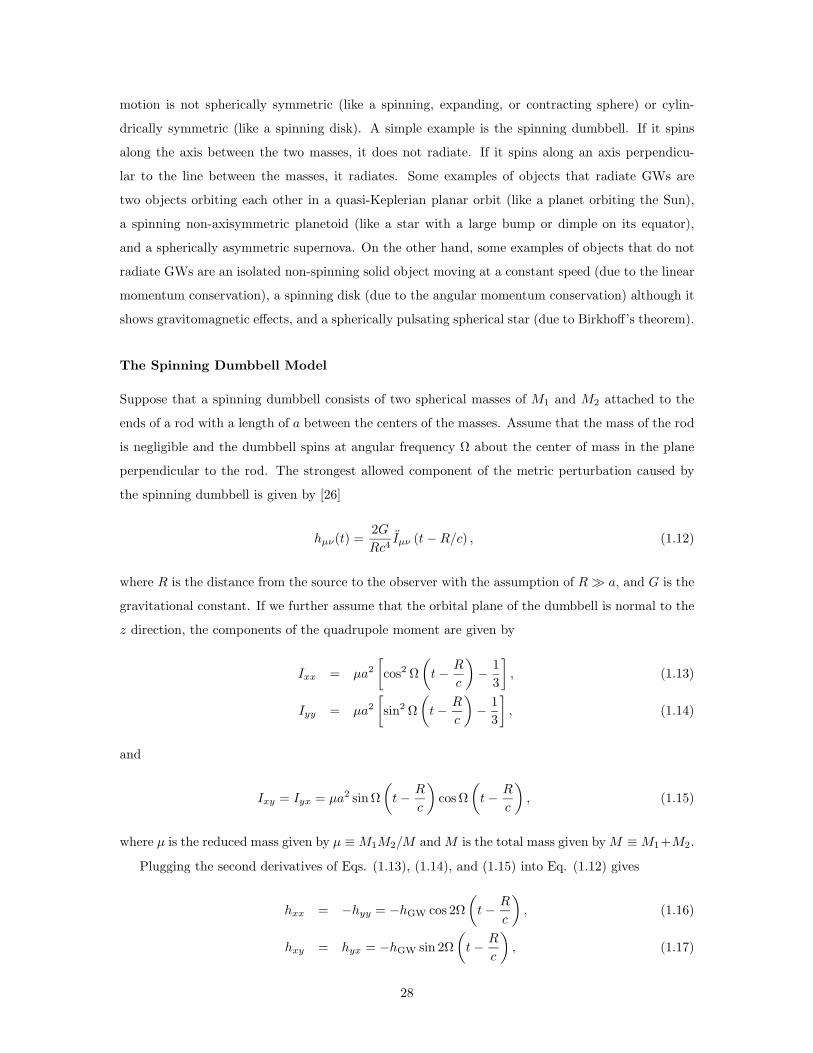
The Spinning Dumbbell Model

Suppose that a spinning dumbbell consists of two spherical masses of M1 and M2 attached to the

ends of a rod with a length of a between the centers of the masses. Assume that the mass of the rod

is negligible and the dumbbell spins at angular frequency Ω about the center of mass in the plane

perpendicular to the rod. The strongest allowed component of the metric perturbation caused by

the spinning dumbbell is given by [26]

hµν(t) =2G

Rc4Iµν (t − R/c) , (1.12)

where R is the distance from the source to the observer with the assumption of R ) a, and G is the

gravitational constant. If we further assume that the orbital plane of the dumbbell is normal to the

z direction, the components of the quadrupole moment are given by

Ixx = µa2

[

cos2 Ω

(

t − R

c

)

− 1

3

]

, (1.13)

Iyy = µa2

[

sin2 Ω

(

t − R

c

)

− 1

3

]

, (1.14)

and

Ixy = Iyx = µa2 sinΩ

(

t − R

c

)

cosΩ

(

t − R

c

)

, (1.15)

where µ is the reduced mass given by µ ≡ M1M2/M and M is the total mass given by M ≡ M1+M2.

Plugging the second derivatives of Eqs. (1.13), (1.14), and (1.15) into Eq. (1.12) gives

hxx = −hyy = −hGW cos 2Ω

(

t − R

c

)

, (1.16)

hxy = hyx = −hGW sin 2Ω

(

t − R

c

)

, (1.17)

28

where hGW is the amplitude of the oscillation given by

hGW =4Gµa2Ω2

Rc4. (1.18)

If it is possible to have an experimental setup that allows extreme parameters such as M1 = M2 =

1000 kg, a = 1 m, Ω/(2π) = 1 kHz, and R = 3000 km (the distance between the LIGO Hanford

Site and the LIGO Livingston Site), then the GW-induced strain at the detector is hGW ∼ 10−37.

Suppose that a bar (or an interferometer with arms) of L = 100 km is used to detect the GW-induced

strain, and then, the induced length change of the bar (or the interferometer) is ∆L = hGWL ∼ 10−32

m. This is extremely small, and below the resolution of any presently known measurement system.

Therefore, it is not technically feasible to generate and detect GWs in a laboratory. For this reason,

in order to detect GWs, we need violent astronomical events in the universe such as coalescences

and collisions of stars and supernova explosions. Astronomical sources of GWs will be described in

the next section.

1.2.3 Astronomical Sources of Gravitational Waves

Overview

A variety of objects and processes in the universe radiate detectable GWs on Earth. They include

(1) inspirals of binary star systems such as neutron star (NS) and black hole (BH) binaries, (2)

pulsars with spin precession, an excited NS oscillation mode, and small distortions of the NS shape

away from axisymmetry, (3) bursts from sources such as stellar collapses, the mergers of compact

binary star systems, the generators of gamma ray bursts, and other energetic phenomena, and

(4) stochastic background from the early universe (cosmological) and the random superposition of

many weak signals from binary star systems (astrophysical). In this section, these GW sources are

discussed.

Inspirals of Binary Star Systems

Radio observations of pulsars confirm the existence of binary NS systems in our Galaxy [27, 28].

General Relativity predicts the decay of a binary orbit due to the emission of gravitational radiation.

The decay rate inferred from observations of PSR1913+16 agrees with the prediction within 0.3%

[29, 30, 31]. Other than PSR1913+16, there are a number of systems known to exhibit orbital decay

in accord with the quadrupole formula [29]. The orbital decay is easily modeled for compact binary

systems containing NSs or stellar mass BHs. The binary orbit is expected to evolve through the

LIGO detection band by the emission of GWs alone, making it possible to accurately compute the

evolution without reference to complicated micro-physics.

29

When a compact binary system first forms, the orbit may be widely separated and highly eccen-

tric. Gravitational radiation causes the orbit to shrink and circularize so that the binary components

eventually spiral together along a sequence of nearly circular orbits [28]. For binary NSs or stellar

mass BHs, the gravitational radiation eventually enters the frequency band of Earth-based GW

detectors. At this point, the orbit decays rapidly and the gravitational waveform chirps upward in

frequency and amplitude, sweeping through the LIGO detection band [32, 33].

For low-mass binary systems, the waveforms are well approximated by a post-Newtonian expan-

sion in the LIGO detection band. If the dumbbell in Sec. 1.2.2 is a binary star system with masses

M1 and M2 with no rod, but the two stars are influenced by the gravitational force between each

other, then the gravitational interaction between the two stars gives a simple expression for the spin

(orbiting) angular frequency Ω =√

GM/a3. The metric perturbation is given in terms of more

physically intuitive quantities by

hGW =rS1rS2

aR, (1.19)

where rS1 and rS2 are the Schwarzschild radii of the stars defined by rS1 ≡ 2GM1/c2 and rS2 ≡

2GM2/c2. A rough estimate for the amplitude of the metric perturbation in Eq. (1.19) is

hGW ∼ 10−21

(

10 km

a

)(

10 Mpc

R

)(

M1

M#

)(

M2

M#

)

. (1.20)

For a NS/NS binary, the typical NS mass is near the Chandrasekhar mass, M1 % M2 % 1.4M#. For

a larger strain amplitude, a and R should be as small as possible.

For a binary star system with eccentricity e, the gravitational luminosity averaged over an orbital

period is given from Eq. (1.11) by

LGW =32

5

G4

c5

µ2M3

a5f(e), (1.21)

where

f(e) =

(

1 +73

24e2 +

37

96e4

)

(1 − e2)−72 (1.22)

is the eccentricity correction function. As the binary system loses energy by gravitational radiation,

the stars spiral in toward each other. For circular orbits (e = 0), the total energy of the system

given by E = −GµM/(2a) decreases as

dE

dt=

GµM

2a2

da

dt= −LGW = −32

5

G4

c5

µ2M3

a5. (1.23)

30

Consequently, the separation between the stars evolves as

a3a = −64

5

G3µM2

c5, (1.24)

which indicates that the rate of decrease in the separation a increases as a decreases. Likewise, using

the orbital angular frequency Ω =√

GM/a3, the orbital period P = 2π/Ω evolves as

P

P= −96

5

G3

c5

µM2

a4, (1.25)

which indicates that P decreases as the separation a decreases.

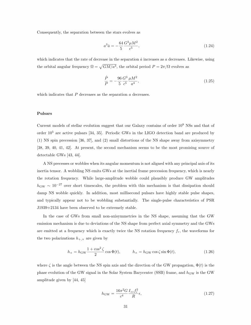
Pulsars

Current models of stellar evolution suggest that our Galaxy contains of order 109 NSs and that of

order 105 are active pulsars [34, 35]. Periodic GWs in the LIGO detection band are produced by

(1) NS spin precession [36, 37], and (2) small distortions of the NS shape away from axisymmetry

[38, 39, 40, 41, 42]. At present, the second mechanism seems to be the most promising source of

detectable GWs [43, 44].

A NS precesses or wobbles when its angular momentum is not aligned with any principal axis of its

inertia tensor. A wobbling NS emits GWs at the inertial frame precession frequency, which is nearly

the rotation frequency. While large-amplitude wobble could plausibly produce GW amplitudes

hGW ∼ 10−27 over short timescales, the problem with this mechanism is that dissipation should

damp NS wobble quickly. In addition, most millisecond pulsars have highly stable pulse shapes,

and typically appear not to be wobbling substantially. The single-pulse characteristics of PSR

J1939+2134 have been observed to be extremely stable.

In the case of GWs from small non-axisymmetries in the NS shape, assuming that the GW

emission mechanism is due to deviations of the NS shape from perfect axial symmetry and the GWs

are emitted at a frequency which is exactly twice the NS rotation frequency fr, the waveforms for

the two polarizations h+,× are given by

h+ = hGW1 + cos2 ζ

2cosΦ(t), h× = hGW cos ζ sinΦ(t), (1.26)

where ζ is the angle between the NS spin axis and the direction of the GW propagation, Φ(t) is the

phase evolution of the GW signal in the Solar System Barycenter (SSB) frame, and hGW is the GW

amplitude given by [44, 45]

hGW =16π2G

c4

Izzf2r

Rε, (1.27)

31

where R is the distance from the observer to the NS, Izz is its principal moment of inertia about

the rotation axis, and ε ≡ (Ixx − Iyy)/Izz is the equatorial ellipticity.

One possible source of ellipticity is tiny hills in the NS crust, which are supported by crustal

shear stresses. For low-mass X-ray binaries (LMXBs), lateral temperature variations in the crust of

order 0.5% or lateral composition variations of 0.5% in the charge-to-mass ratio could build up NS

ellipticities of order 10−8−10−7. Another possible source of NS ellipticity is strong internal magnetic

fields. Toroidal magnetic fields of order 1012 − 1013 G would lead to sufficient GW emission to halt

the spin-up of LMXBs and account for the observed spin-down of millisecond pulsars [46].

A simple model of a pulsar is 1.4M# NS of radius 10 km with the principal moment of inertia

about the rotation axis Izz = 1045 g cm2 and the magnetic field B ∼ 1012 G. Then, a rough estimate

for the GW amplitude is given by

hGW ∼ 10−31

(

fr

1 kHz

)2 (10 kpc

R

)

. (1.28)

If pulsars are born rapidly rotating, then there should be several of the most recent pulsars with

such an amplitude present in our Galaxy at any time.

Bursts

GW bursts are expected to be produced from catastrophic phenomena in the universe such as stellar

collapses, the mergers of compact binary star systems as they form a single body, the generators of

gamma ray bursts, and other energetic phenomena [47, 48, 33, 49, 50, 51]. Perturbed or accreting

BHs, NS oscillation modes and instabilities, as well as cosmic string cusps and kinks are also potential

burst sources. The expected rate, strength, and waveform morphology for such events are poorly

known.

Stochastic Background

A stochastic background of gravitational radiation is analogous to the cosmic microwave background

radiation although its spectrum is unlikely to be thermal [52]. Sources of a stochastic background

could be cosmological or astrophysical in origin. Examples of the former are zero-point fluctuations

of the spacetime metric amplified during inflation, and first-order phase transitions and decaying

cosmic string networks in the early universe [52, 53, 54, 55]. An example of an astrophysical source is

the random superposition of an extremely large number of unresolved and independent GW emission

events [52, 53, 56].

The spectrum of a stochastic background is usually described by the dimensionless quantity

ΩGW(f) which is the GW energy density per unit logarithmic frequency ρGW, divided by the critical

32

energy density ρc to close the universe,

ΩGW(f) ≡ f

ρc

dρGW

df, (1.29)

where the critical density is ρc ≡ 3c2H20/(8πG) and H0 is the present day Hubble expansion rate.

The measurable (one-sided) power spectrum of the GW strain SGW(f) is given by [57]

SGW(f) =3H2

0

10π2f−3ΩGW(f). (1.30)

For a stochastic GW background with ΩGW(f) ≡ Ω0 (constant) as is predicted in the LIGO detection

band by inflationary models in the infinitely slow-roll limit or by cosmic string models [58, 54], the

power in GWs falls off as 1/f3 [57, 56]. A rough estimate for the GW strain amplitude in this case

is given by

hGW(f) =√

SGW(f) = 5.6 × 10−22h100

√

Ω0

(

100 Hz

f

)3/2

Hz−1/2, (1.31)

where h100 ≡ H0/H100 and H100 ≡ 100 km/s/Mpc. Here we have assumed that the stochastic

background is isotropic, unpolarized, stationary, and Gaussian.

1.3 Laser-Interferometric Gravitational-Wave Detectors

1.3.1 The History of Gravitational-Wave Detectors

As stated already, GWs are ripples in the fabric of spacetime, and therefore, a passing GW changes

the separation of adjacent test masses. This tidal effect is the basis of all present GW detectors. The

great challenge of this type of detection, though, is the extraordinarily small effect that GWs would

produce on a detector. The amplitude of any wave falls off as the inverse of the distance from the

source. Thus, even GWs from merging binary BHs die out to a very small amplitude by the time

they reach the Earth. For GW sources occurring with a reasonable observation rate, the predicted

magnitude of the GW amplitude in the vicinity of the Earth is extremely small, on the order of

hGW ∼ 10−21 or lower. In fact, current theoretical models on the event rate and strength of such

events suggest that an amplitude sensitivity of 10−22 over a time scale of 1 ms is required to detect

a few GW events per year (such as coalescing NS binaries). In other words, if the Fourier spectrum

of a possible GW signal is considered, the required spectral density of the amplitude sensitivity for

the 1 ms time scale is 10−22/√

1000 Hz % 3× 10−24/√

Hz over the frequency range of the signal. To

detect such a small effect, several detection techniques have been proposed: resonant bar detectors

[59, 60] and interferometers such as Michelson interferometers [3, 1], Sagnac interferometers [61],

atom interferometers [62, 63], and displacement-noise-free interferometers [25, 64].

33

A resonant bar detector or the so-called Weber bar [59] is composed of a large cylindrical bar with

transducers attached to detect any vibrations. This type of instrument was the first type of GW

detector. The idea is that a passing GW rings up the bar at its resonant frequency, which basically

amplifies the wave naturally. Alternatively, a nearby supernova might be strong enough to be seen

without resonant amplification. Modern forms of the bar detector are still operated, cryogenically

cooled, with superconducting quantum interference devices to detect the motion. Unfortunately,

one downside of bar detectors is that their sensitivity is limited to very narrow bandwidths.

The rough idea of a laser-interferometric GW detector was found by Pirani in 1956 [65]. Later,

the first explicit suggestion of such a detector was made by Gertsenshtein and Pustovoit in 1962 [66].

In the mid-1960s, Weber [59], unaware of the work done by Gertsenshtein and Pustovoit, reinvented

the idea, but left it in his laboratory notebook unpublished and unpursued. In 1970, Weiss at

MIT, unaware of the work done by Gertsenshtein and Pustovoit or Weber, reinvented the idea and

carried out a detailed design and feasibility study [67], which is currently used in the operational

GW detectors such as Laser Interferometer Gravitational-Wave Observatory (LIGO) [1], VIRGO

[4], GEO600 [5], and TAMA300 [6]. The biggest advantage of interferometric detectors over bar

detectors is their broadband sensitivity that allows for detection of GWs at all frequencies in the

GW detection band.

1.3.2 The Principle of Laser-Interferometric Gravitational-Wave Detec-

tors

The basic principle of a Michelson interferometer as a GW detector is given by the postulate that

the infinitesimal spacetime interval ds for light is zero, or

ds2 = 0. (1.32)

This is the key that makes it possible for us to detect GWs with a Michelson interferometer [1, 3, 26].

Consider a Michelson interferometer that consists of a laser at frequency ω, a beamsplitter, two

test mass mirrors with equal arm lengths of L, and a photodetector as shown in Fig. 1-1. Assume

that the beamsplitter is perfectly balanced and lossless and the mirrors are perfectly reflecting and

lossless. Suppose, without the loss of generality, that the Michelson interferometer is set up such

that its two arms are aligned along the x and y axes and then, only the h+ polarization of the GW is

considered. Moreover, assume that the curvature of spacetime where the Michelson interferometer

is located is weak so that the weak-field limit in Eq. (1.3) can be used.

Consider that the laser travels in the arm along the x axis. The infinitesimal spacetime interval

34

LASER

Photodetector

Test Mass x

Test Mass y

L

L

Beamsplitter

Figure 1-1: A Michelson interferometer that consists of a laser at frequency ω, a beamsplitter, twotest mass mirrors with an equal arm length of L, and a photodetector.

ds that the laser travels is given by

ds2 = 0 = gµνdxµdxν % (ηµν + hµν)dxµdxν

= −c2dt2 + [1 + hxx (t − eZ · x/c)] dx2, (1.33)

which indicates that the passing GW modulates the infinitesimal spacetime interval in the x arm by

a fractional amount of hxx. The light travel time from the beamsplitter to the x test mass mirror

is, hence, given by

∫ τx1

0dt =

1

c

∫ L

0

√

1 + hxx (t − eZ · x/c)dx % 1

c

∫ L

0

[

1 +1

2hxx (t − eZ · x/c)

]

dx, (1.34)

where we have assumed that hxx + 1. Likewise, the light travel time from the x test mass mirror

to the beamsplitter (for the round-trip) is given by

∫ τx2

0dt = −1

c

∫ 0

L

√

1 + hxx (t − eZ · x/c)dx % −1

c

∫ 0

L

[

1 +1

2hxx (t − eZ · x/c)

]

dx. (1.35)

Therefore, the total round-trip time is found to be

τxtot = τx1 + τx2 % 2L

c+

1

c

∫ L

0hxx (t − eZ · x/c) dx. (1.36)

Similarly, the total round-trip time between the beamsplitter and the y test mass mirror for the

35

laser that travels along the y arm is given by

τytot %2L

c+

1

c

∫ L

0hyy (t − eZ · x/c) dy. (1.37)

The photodetector at the interferometer output measures change in the interference of the two

laser beams induced by the passing GW. If the input electric field to the beamsplitter is E0, assuming

that any common constant phase or reflection-induced constant phase shift is absorbed into the

amplitudes of the electric fields, the interferometer output field at the beamsplitter is given by

E =1

2E0

(

eiωτxtot − eiωτytot)

% i

2E0φGW, (1.38)

where

φGW(t) = ω(τxtot − τytot) %ω

c

∫ L

0[hxx (t − eZ · x/c) dx − hyy (t − eZ · x/c) dy] . (1.39)

is the GW-induced phase shift. If we assume that the GW propagates along the z axis so that

eZ = ez, then hxx = −hyy ≡ hGWeiΩt and eZ · x = 0. Under this assumption, the phase shift can

be simplified to the expression [26]

φGW(t) = hGW(t)4πL

λ

sin(ΩL/c)

ΩL/ceiΩL/c (1.40)

where Ω/(2π) is the frequency of the GW and λ is the laser wavelength. Eq. (1.40) indicates that

in order to measure an extremely small value of hGW(t) on the order of 10−22, large L and short λ

are required.

1.4 Quantum Noise in Gravitational-Wave Detectors

1.4.1 Introduction

Although there are several noise sources that limit the sensitivity of laser-interferometric GW de-

tectors, such as seismic [68, 69, 70, 71, 72] and thermal noise [73, 74, 75, 76, 77, 78, 79, 80, 81],

the detector sensitivity is ultimately limited by quantum noise that comes from the quantum nature

of photons due to the Heisenberg uncertainty principle. The limiting quantum noise sources of the

GW detectors are (1) photon shot noise that arises from uncertainty due to quantum mechanical

fluctuations in the number of photons at the interferometer output and (2) quantum radiation pres-

sure noise that arises from mirror displacements induced by quantum radiation pressure fluctuations

[82, 83]. Shot noise and radiation pressure noise1 dominate in different frequency bands. Radiation

1Quantum radiation pressure noise is often shortened to radiation pressure noise in the GW community. It shouldnot be confused with classical radiation pressure noise.

36

pressure noise exerts a force on the interferometer mirrors, which respond to the force only at low

frequencies due to the mechanical susceptibility. Shot noise dominates at higher frequencies where

the mirror response to radiation pressure noise becomes smaller. Both shot noise and radiation

pressure noise are caused by quantum fluctuations of a vacuum electromagnetic field that enters the

unused or antisymmetric port of the interferometers [84]. Shot and radiation pressure noises are

manifestations of the two quadratures of the vacuum.

The sensitivities of the currently operational laser-interferometric GW detectors such as LIGO

[1], VIRGO [4], GEO600 [5], and TAMA300 [6] are already limited by such quantum noise at high

frequencies in the GW detection band (10 Hz - 10 kHz). Next generation GW detectors such as

Advanced LIGO [7], which are planned to be operational in the next few years, are also expected to

be limited by quantum noise at almost all frequencies in the GW detection band [82].

In the following sections, the origin of the quantum noise in GW detectors is described. The

Heisenberg uncertainty principle is reviewed in the quantum optical picture, and then, photon shot

noise and quantum radiation pressure noise are derived based on it. The quantum noise in LIGO

and Advanced LIGO is also shown to see how it limits the detector sensitivities. Finally, the most

rigorous derivation of the quantum noise is briefly introduced and will be fully described in Chap.

5.

1.4.2 The Heisenberg Uncertainty Principle

The Heisenberg uncertainty principle introduced by Heisenberg in 1927 states that it is fundamen-

tally impossible to simultaneously obtain the precise knowledge of two non-commuting observables

[85]. For observables A and B, if the commutation relation,

[A,B] = AB − BA, (1.41)

is a non-zero constant, the product of the uncertainties of simultaneous measurements on the ob-

servables is bounded by

∆A∆B ≥ 1

2| 〈[A,B]〉 |, (1.42)

where

〈O〉 = 〈Ψ|O |Ψ〉 (1.43)

is the operator mean of observable O in the system state Ψ and

∆O ≡√

⟨

(O − 〈O〉)2⟩

=√

〈O2〉 − 〈O〉2 (1.44)

37

is the operator standard deviation of observable O in the system state Ψ.

The most common example of the Heisenberg uncertainty principle is the position and momentum

of a free particle. The better position is known, the less well the momentum is known, and vice versa.

This principle also applies to a particle trapped in a harmonic potential. The particle oscillates in the

potential simple-harmonically. This situation is analogous to the oscillation of an electromagnetic

field at frequency ω. In the Heisenberg picture, an electromagnetic field characterized by its field

annihilation operator a and its field creation operator a† satisfies the commutation relation [86, 87,

88]

[

a, a†] = 1. (1.45)

Following the commutation relation, the two observable quadrature fields (the so-called amplitude

and phase quadratures) defined by [88, 89]

a1 ≡ a + a† Amplitude Quadrature, (1.46)

a2 ≡ −i(

a − a†) Phase Quadrature, (1.47)

form an arbitrary quadrature operator,

aθ ≡ ae−iθ + a†eiθ = a1 cos θ + a2 sin θ. (1.48)

From Eq. (1.45), the commutation relation of the observables is given by

[a1, a2] = 2i. (1.49)

Therefore, for the observables a1 and a2, Eq. (1.42) leads to the uncertainty relation,

∆a1∆a2 ≥ 1, (1.50)

from which, we can see that it is impossible to simultaneously measure the amplitude and phase

quadratures of an optical field with 100% accuracy. The ground state of an electromagnetic field is a

vacuum state or the state with no average photons in it, and is represented by |0〉 in the Schrodinger

picture. Even if there is no average number of photons in the vacuum state, it has fluctuations in

both amplitude and phase quadratures and their variances are equal since they are indistinguishable.

38

1.4.3 Quantum Noise Sources

Photon Shot Noise

Photon shot noise is the direct consequence of the quantum nature of photons. Measuring the

power of an electromagnetic field is equivalent to determining the number of photons arriving at a

photodetector during a measurement time interval. A coherent state |α〉 is defined as the eigenstate

of the annihilation operator [90, 89],

a |α〉 = α |α〉 . (1.51)

The coherent state can be obtained by applying the displacement operator [89]

D (α) ≡ e−12 |α|

2

eαa†−α∗a (1.52)

to a vacuum state |0〉, such that

D(α) |0〉 = |α〉 , (1.53)

which yields the coherent state in the basis of Fock or number states |n〉,

|α〉 = e−12 |α|

2∞∑

n=0

αn

√n!

|n〉 . (1.54)

The photon number probability distribution is therefore found to be

P (n) = |〈n|α〉|2 =〈n〉n e−〈n〉

n!, (1.55)

where 〈n〉 =⟨

a†a⟩

= |α|2 is the average photon number. Eq. (1.55) is also called the Poisson

distribution or often referred to as counting statistics. When 〈n〉 ) 1, the Poisson distribution can

be approximated by a Gaussian distribution with the standard deviation given by

∆n =√

〈n2〉 − 〈n〉2 = |α| =√

〈n〉. (1.56)

In a Michelson interferometer as shown in Fig. 1-1, the average photon number per unit time at

the output of the interferometer is given by

⟨

dn

dt

⟩

=λ

2πhcPout, (1.57)

and therefore, the standard deviation of the average photon number detected for a time interval of

39

τ is given by

∆n =√

〈n〉 =

√

⟨

dn

dt

⟩

τ =

√

λPoutτ

2πhc. (1.58)

Since we are using the power of the interferometer output as a monitor of the differential position

of the two test masses, we can obtain the displacement fluctuations by setting the optical power

fluctuations as equivalent to position difference fluctuations, given by the fractional photon number

fluctuation divided by the fractional output power change per unit position difference. Assuming

that we are interested in the linear response of the detector at the mid-fringe of the interferometer

(Pout|mid−fringe = Pin/2) under the condition ΩL/c + 1 so that the detector response in Eq. (1.40)

is flat in the band, the standard deviation in the displacement L due to fluctuations in the average

photon number detected for a time interval of τ is given by

∆Lshot =∆n/ 〈n〉1

Pout

dPoutdL

=

√

hcλ

4πPinτ. (1.59)

In the frequency domain defined by

O(t) =1

2π

∫ ∞

−∞O(Ω)eiΩtdΩ for an operator O(t), (1.60)

where Ω is the sideband frequency relative to the carrier frequency, the strain noise caused by the

photon shot noise in terms of the equivalent GW noise is thus found to be

hshot(Ω) =∆Lshot(Ω)

L=

1

L

√

hcλ

2πPin, (1.61)

where we have used a factor of√

2 from our preference for one-sided spectra. It is important to note

that Eq. (1.61) is frequency-independent and thus, flat in the frequency domain. Increasing the

input laser power Pin can improve the strain associated with the shot noise and thus enhance the

detector sensitivity at all frequencies. However, this is not the case due to the presence of quantum

radiation pressure noise that scales as√

Pin, which will be discussed later in this section.

Shot noise is currently the limiting noise source at frequencies above 100 Hz in the LIGO detectors

[91] and is also expected to be one of the dominant limiting noise sources in Advanced LIGO [7]. In

displacement-noise-free interferometers [25], shot noise is the only limiting fundamental noise source

and therefore, reducing the shot noise directly improves the detector sensitivity at all frequencies in

the GW detection band.

40

Quantum Radiation Pressure Noise

The optical measurement of the position of an interferometer test mass is analogous to the mea-

surement of a particle with light, the so called Heisenberg microscope, in which the registration of

the arrival of a photon that bounces off the particle is a measure of the recoil of the particle caused

by the change in the momentum of the photon upon reflection. In a Michelson interferometer as

shown in Fig. 1-1, we register an arrival rate of photons that we interpret as a measurement of the

difference in phase between optical fields returning from the two arms.

The force exerted by an optical field of power Pm perfectly reflecting normally from a lossless

mirror test mass in each interferometer arm is given by

Frad =2Pm

c=

Pin

c, (1.62)

where we have used Pm = Pin/2 since the beamsplitter splits the input power equally. The fluctuation

in this force is caused by shot noise fluctuation in Pin given by

∆Pin = hω∆n = hω√

〈n〉 =

√

2πchPinτ

λ(1.63)

as discussed early in this section, so that in the frequency domain, it is given by

∆Frad(Ω) =∆Pin(Ω)

c=

√

2πhPin

cλ, (1.64)

which is frequency-independent. Assuming that the beamsplitter is much more massive than the

two mirror test masses, the mirror position fluctuation caused by the radiation pressure fluctuation

is given by

∆Lrad(Ω) =1

mΩ2∆Frad(Ω) =

1

mΩ2

√

2πhPin

cλ. (1.65)

The power fluctuations in the two arms are anti-correlated, meaning that when one additional photon

goes into one arm, one less photon goes into the other arm, doubling the effect on the output of the

interferometer. Therefore, the strain noise caused by the radiation pressure noise in terms of the

equivalent GW noise is found to be

hrad(Ω) =2∆Lrad(Ω)

L=

1

mΩ2L

√

8πhPin

cλ, (1.66)

which scales as Ω−2 due to the frequency response of the suspended mirrors, and is hence significant

at low frequencies. It is important to note that unlike the shot noise, the radiation pressure noise

increases with increasing Pin. Shot noise and radiation pressure noise are both shown in Fig. 1-2.

41

10−3 10−2 10−1 10010−26

10−25

10−24

10−23

10−22

10−21

10−20

10−19

Frequency (Hz)

Stra

in (H

z−1/

2 )

Shot Noise

Radiation Pressure Noise

Total Quantum Noise

Figure 1-2: Shot noise and quantum radiation pressure noise in a Michelson interferometer. Thetest mass, input laser power, laser wavelength, and arm length used for the figure are m = 10 kg,Pin = 5 W, λ = 1064 nm, and L = 500 km. At high frequencies, the shot noise dominates whereasat low frequencies, the radiation pressure noise dominates due to its f−2 dependence.

Standard Quantum Limit

The total quantum noise of a Michelson interferometer, or the so-called optical readout noise, is the

quadrature sum of the shot noise and radiation pressure noise,

htot(Ω) =√

h2shot(Ω) + h2

rad(Ω). (1.67)

At low frequencies, the radiation pressure noise dominates whereas at high frequencies, the shot

noise dominates. In addition, the shot noise decreases as the input power Pin increases whereas the

radiation pressure increases with larger Pin. If the total quantum noise is minimized with respect

to the input power Pin, the minimum noise or the so-called standard quantum limit (SQL) is found

to be [83, 92, 93, 94],

hSQL(Ω) =

√

4h

mΩ2L2, (1.68)

at the optimum power PSQL = cλmΩ2/(4π). Since this expression does not depend on Pin or λ, or

any other feature of the readout scheme, it hence places the ultimate quantum limit on precision

measurement.

42

1.4.4 Quantum Noise in LIGO and Advanced LIGO

Advanced Interferometer Configurations

Present day and next generation GW detectors utilize more complex interferometer configurations

than the simple Michelson interferometer. For example, as shown in Fig. 1-3, a power-recycled

Fabry-Perot Michelson interferometer (PRFPMI) configuration is used in LIGO [91] and a dual-

recycled (power-recycled and signal-recycled) Fabry-Perot Michelson interferometer (DRFPMI) con-

figuration is planned for Advanced LIGO [7].

(b)(a)

LASER

Photodetector

ArmCavity

BS

ArmCavity

PRM

LASER

Photodetector

ArmCavity

BS

ArmCavity

SRM

PRM

Figure 1-3: Interferometer configurations: (a) a power-recycled Fabry-Perot Michelson (PRFPMI)interferometer and (b) a dual-recycled (power-recycled, signal-recycled) Fabry-Perot Michelson(DRFPMI) interferometer. PRM: power-recycling mirror, SRM: signal-recycling mirror, BS: beam-splitter. The PRFPMI interferometer configuration is used in LIGO and the DRFPMI configurationis planned for Advanced LIGO.

Fabry-Perot cavities in the arms of the Michelson interferometer increase the light storage time

of the arms. The strain sensitivity of the Michelson interferometer at frequencies limited by shot

noise can also be enhanced by increasing the laser power incident on the beamsplitter. Since the

interferometer is operated on a dark fringe so that the laser power which is not lost to absorption,

scattering, or leakage out of the dark port goes back to the laser source, a partially transmitting

mirror2 can be inserted in between the laser source and the beamsplitter to recycle the laser back

into the interferometer. This mirror, which is conventionally called a power-recycling mirror (PRM),

and the interferometer form a power-recycling cavity (PRC). Likewise, a mirror can also be inserted

between the beamsplitter and photodetector to recycle the GW-induced phase shift back into the

interferometer (with optimization and limitations due to the losses in the interferometer). This

mirror, which is conventionally called a signal-recycling mirror (SRM), and the interferometer form

2The mirror transmission is equal to the interferometer losses.

43

a signal-recycling cavity (SRC). Details of the advanced interferometer configurations can be found

in Refs. [82, 95, 96, 7, 1].

Conventional Gravitational Wave Detectors such as LIGO

For a conventional GW detector with arm lengths L and mirror masses m in the PRFPMI configu-

ration, the quantum noise in the GW strain signal is given by [82]

h(Ω) =hSQL√

2

√

K +1

K , (1.69)

where

hSQL(Ω) =

√

8h

mΩ2L2(1.70)

is the SQL3, and K is the effective coupling constant that relates motion of the mirrors to the output

signal, given by4

K =2γ4

Ω2(γ2 + Ω2)

Pin

PSQL. (1.71)

Here γ is the linewidth of the arm cavities (typically γ ∼ 2π × 100 Hz), and PSQL is the input laser

power required to reach the SQL in the PRFPMI detector, given by PSQL = mL2γ4/(4ω). Assuming

that Pin = PSQL, if Ω + γ, then K ) 1/K, and thus,

h(Ω) % hSQLγ

Ω=

1

Ω2

√

8hγ2

mL2, (1.72)

which indicates that the radiation pressure noise dominates in the band. If Ω ) γ, then 1/K ) K,

and thus,

h(Ω) % hSQLΩ2

2γ2= Ω

√

2h

mL2γ4, (1.73)

which indicates that the shot noise dominates in the band. The frequency dependence of the shot

noise and radiation pressure noise in the PRFPMI detector is shown in Fig. 1-4.

Fig. 1-4 also shows the sensitivities of all the currently operational LIGO interferometers [97].

They are limited by shot noise at frequencies above ∼200 Hz. Radiation pressure noise is completely

masked by seismic noise [68], thermal noise [79, 80, 81], and control noise [98] at low frequencies.

3This is a factor of√

2 different from the SQL in Eq. (1.68) because in this interferometer with Fabry-Perot cavityarms, the effect is doubled by the cavities formed by two mirrors in each arm.

4Since the power-recycling gain of a conventional GW detector is typically constant in the LIGO detection band(10 Hz - 10 kHz), it is absorbed into the input laser power to the beamsplitter Pin, such that Pin is not the laserpower to the PRM, but to the beamsplitter.

44

101 102 103 10410−24

10−23

10−22

10−21

10−20

10−19

10−18

10−17

Frequency (Hz)

Stra

in (H

z−1/

2 )

LHO 4km (2006.03.13)LLO 4km (2006.06.04)LHO 2km (2006.06.18)Seismic NoiseThermal NoiseQuantum NoiseLIGO Goal 4km (Total Noise)

Figure 1-4: The strain sensitivity of the LIGO interferometers during the S5 science run. LHO 4km:LIGO Hanford 4 km Detector, LHO 2km: LIGO Hanford 2 km Detector, LLO: LIGO LivingsonDetector. The neutron star binary inspiral range for 1.4M#/1.4M# neutron stars is 14.5 Mpc forLHO 4km, 15.1 Mpc for LLO 4km, and 7.4 Mpc for LHO 2km [97]. For all the detectors, shot noiseis the limiting noise source at frequencies above 200 Hz.

Since the radiation pressure noise is not significant, increasing the laser power can simply increase

the sensitivity at frequencies above ∼200 Hz although higher laser power can lead to problems with

thermal loading (deformations of the interferometer mirrors due to absorbed laser power) [1, 99, 100].

Next Generation Gravitational Wave Detectors such as Advanced LIGO

For a next generation GW detector in the DRFPMI configuration with a detuned SRC, the quantum

noise in the GW strain signal is given by [96]

h(Ω) = hSQL

√

(C11 sin ζ + C21 cos ζ)2 + (C12 sin ζ + C22 cos ζ)2

2Kt2SRM|D1 sin ζ + D2 cos ζ|2 , (1.74)

where ζ is the homodyne phase5,

C11 = C22 = (1 + r2s)

(

cos 2φ +K2

sin 2φ

)

− 2rs cos[2(β + Φ)], (1.75)

C12 = −t2s(sin 2φ + K sin2 φ), C21 = t2s(sin 2φ−K cos2 φ), (1.76)

D1 = −(

1 + rse2i(β+Φ)

)

sinφ, D2 = −(

−1 + rse2i(β+Φ)

)

cosφ, (1.77)

5This definition of the homodyne phase is slightly different in meaning from that in the field of quantum optics.

45

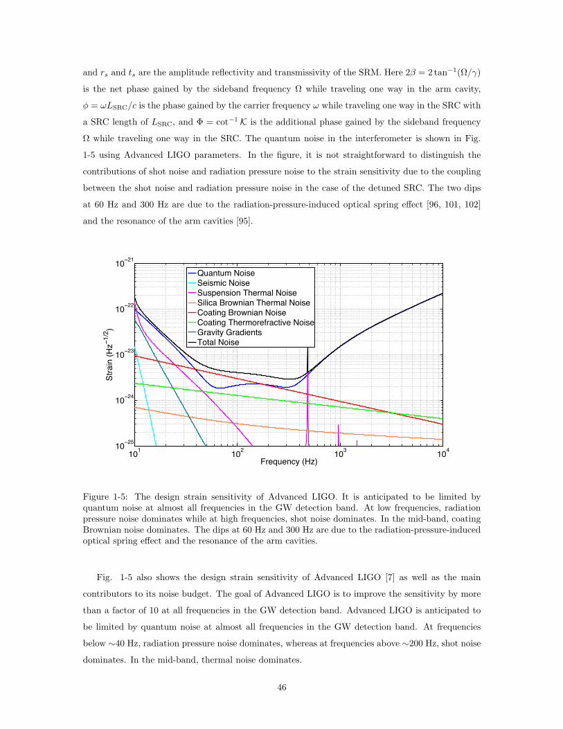
and rs and ts are the amplitude reflectivity and transmissivity of the SRM. Here 2β = 2 tan−1(Ω/γ)

is the net phase gained by the sideband frequency Ω while traveling one way in the arm cavity,

φ = ωLSRC/c is the phase gained by the carrier frequency ω while traveling one way in the SRC with

a SRC length of LSRC, and Φ = cot−1 K is the additional phase gained by the sideband frequency

Ω while traveling one way in the SRC. The quantum noise in the interferometer is shown in Fig.

1-5 using Advanced LIGO parameters. In the figure, it is not straightforward to distinguish the

contributions of shot noise and radiation pressure noise to the strain sensitivity due to the coupling

between the shot noise and radiation pressure noise in the case of the detuned SRC. The two dips

at 60 Hz and 300 Hz are due to the radiation-pressure-induced optical spring effect [96, 101, 102]

and the resonance of the arm cavities [95].

101 102 103 10410−25

10−24

10−23

10−22

10−21

Frequency (Hz)

Stra

in (H

z−1/

2 )

Quantum NoiseSeismic NoiseSuspension Thermal NoiseSilica Brownian Thermal NoiseCoating Brownian NoiseCoating Thermorefractive NoiseGravity GradientsTotal Noise

Figure 1-5: The design strain sensitivity of Advanced LIGO. It is anticipated to be limited byquantum noise at almost all frequencies in the GW detection band. At low frequencies, radiationpressure noise dominates while at high frequencies, shot noise dominates. In the mid-band, coatingBrownian noise dominates. The dips at 60 Hz and 300 Hz are due to the radiation-pressure-inducedoptical spring effect and the resonance of the arm cavities.

Fig. 1-5 also shows the design strain sensitivity of Advanced LIGO [7] as well as the main

contributors to its noise budget. The goal of Advanced LIGO is to improve the sensitivity by more

than a factor of 10 at all frequencies in the GW detection band. Advanced LIGO is anticipated to

be limited by quantum noise at almost all frequencies in the GW detection band. At frequencies

below ∼40 Hz, radiation pressure noise dominates, whereas at frequencies above ∼200 Hz, shot noise

dominates. In the mid-band, thermal noise dominates.

46

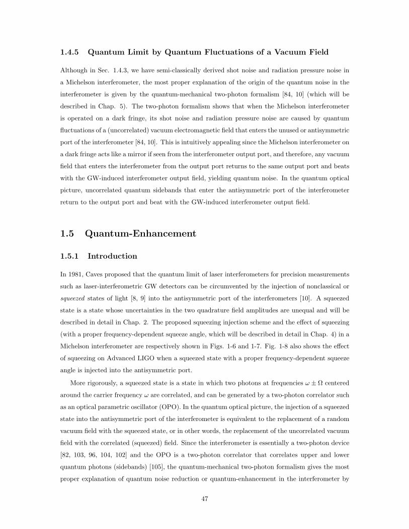
1.4.5 Quantum Limit by Quantum Fluctuations of a Vacuum Field

Although in Sec. 1.4.3, we have semi-classically derived shot noise and radiation pressure noise in

a Michelson interferometer, the most proper explanation of the origin of the quantum noise in the

interferometer is given by the quantum-mechanical two-photon formalism [84, 10] (which will be

described in Chap. 5). The two-photon formalism shows that when the Michelson interferometer

is operated on a dark fringe, its shot noise and radiation pressure noise are caused by quantum

fluctuations of a (uncorrelated) vacuum electromagnetic field that enters the unused or antisymmetric

port of the interferometer [84, 10]. This is intuitively appealing since the Michelson interferometer on

a dark fringe acts like a mirror if seen from the interferometer output port, and therefore, any vacuum

field that enters the interferometer from the output port returns to the same output port and beats

with the GW-induced interferometer output field, yielding quantum noise. In the quantum optical

picture, uncorrelated quantum sidebands that enter the antisymmetric port of the interferometer

return to the output port and beat with the GW-induced interferometer output field.

1.5 Quantum-Enhancement

1.5.1 Introduction

In 1981, Caves proposed that the quantum limit of laser interferometers for precision measurements

such as laser-interferometric GW detectors can be circumvented by the injection of nonclassical or

squeezed states of light [8, 9] into the antisymmetric port of the interferometers [10]. A squeezed

state is a state whose uncertainties in the two quadrature field amplitudes are unequal and will be

described in detail in Chap. 2. The proposed squeezing injection scheme and the effect of squeezing

(with a proper frequency-dependent squeeze angle, which will be described in detail in Chap. 4) in a

Michelson interferometer are respectively shown in Figs. 1-6 and 1-7. Fig. 1-8 also shows the effect

of squeezing on Advanced LIGO when a squeezed state with a proper frequency-dependent squeeze

angle is injected into the antisymmetric port.

More rigorously, a squeezed state is a state in which two photons at frequencies ω ± Ω centered

around the carrier frequency ω are correlated, and can be generated by a two-photon correlator such

as an optical parametric oscillator (OPO). In the quantum optical picture, the injection of a squeezed

state into the antisymmetric port of the interferometer is equivalent to the replacement of a random

vacuum field with the squeezed state, or in other words, the replacement of the uncorrelated vacuum

field with the correlated (squeezed) field. Since the interferometer is essentially a two-photon device

[82, 103, 96, 104, 102] and the OPO is a two-photon correlator that correlates upper and lower

quantum photons (sidebands) [105], the quantum-mechanical two-photon formalism gives the most

proper explanation of quantum noise reduction or quantum-enhancement in the interferometer by

47

LASER

SqueezedState

OpticalCirculator

Photodetector

MichelsonInterferometer

Figure 1-6: A schematic of a Michelson interferometer with squeezing injected into the antisymmetricport of the interferometer via the optical circulator. The squeezing-enhanced interferometer fieldwith a possible gravitational wave signal that beats against it is detected by the photodetector.

squeezing, which will be described in detail in Chap. 5.

1.5.2 Ideal Squeezed State Production and Quantum Enhancement

In this section, a squeezed state, or more rigorously a squeezed coherent state, is conceptually obtained

by use of operators. Suppose that we have a two-photon squeeze operator for two photons (upper

and lower sideband photons) or the so-called signal and idler fields [as(ω + Ω) and ai(ω −Ω)] with

respect to the carrier frequency ω (without worrying about the physical origin of the operator for

the moment) [105]

Ssi(ξ) ≡ eξ∗asai−ξa†

sa†i , (1.78)

where ξ = reiφ. Here r is the squeeze factor and φ is the squeeze angle. In addition, the displacement

operators for the signal and idler fields [Ds(αs) and Di(αi)] are given in Eq. (1.52). A squeezed

coherent state is obtained by acting with the displacement operators [Ds(αs) and Di(αi)] on the

two-photon vacuum state |0, 0〉 followed by the squeeze operator Ssi(ξ) [106, 105], such that

|αs,αi, ξ〉 = Ssi(ξ)Ds(αs)Di(αi) |0, 0〉 . (1.79)

48

10−3 10−2 10−1 10010−24

10−23

10−22

10−21

10−20

10−19

Frequency (Hz)

Stra

in (H

z−1/

2 )

Quantum Noise

Squeezed Quantum Noise

Figure 1-7: The effect of squeezing on a Michelson interferometer when a squeezed vacuum fieldwith a proper frequency-dependent squeeze angle (which will be described in detail in Chap. 4) isinjected into the antisymmetric port. The test mass, input laser power, laser wavelength, and armlength used for the figure are m = 10 kg, Pin = 5 W, λ = 1064 nm, and L = 500 km. The effect ofsqueezing is assumed to be quantum noise reduction by 20 dB or increase in strain sensitivity by afactor of 10.

Using the useful unitary transformation properties of the squeeze operator [89, 88]

S†si(ξ)asSsi(ξ) = as cosh r − a†

ieiφ sinh r, (1.80)

S†si(ξ)aiSsi(ξ) = ai cosh r − a†

seiφ sinh r, (1.81)

we find the quadrature variances of a1 and a2 [105],

V1(r,φ) ≡ (∆a1)2 =

⟨

|a1 − 〈a1〉|2⟩

= cosh 2r −√

1 − Ω2

ω2sinh 2r cos 2φ, (1.82)

V2(r,φ) ≡ (∆a2)2 =

⟨

|a2 − 〈a2〉 |2⟩

= cosh 2r +

√

1 − Ω2

ω2sinh 2r cos 2φ. (1.83)

Fig. 1-9 shows the quadrature variances of a1 and a2 as a function of φ. The periodic dependence

of squeezing and anti-squeezing on φ is evident.

If Ω/ω + 1, which is often the case since Ω/(2π) ∼ 10 kHz at most and ω/(2π) = c/λ, where λ

49

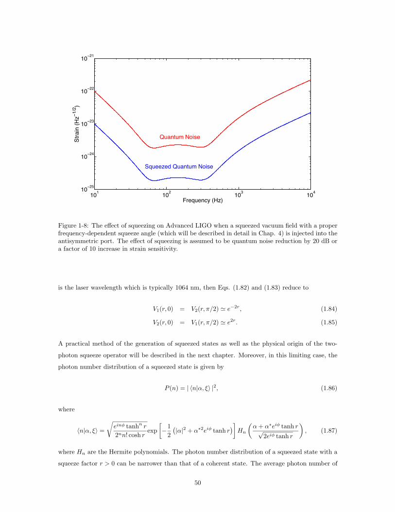
101 102 103 10410−25

10−24

10−23

10−22

10−21

Frequency (Hz)

Stra

in (H

z−1/

2 )

Quantum Noise

Squeezed Quantum Noise

Figure 1-8: The effect of squeezing on Advanced LIGO when a squeezed vacuum field with a properfrequency-dependent squeeze angle (which will be described in detail in Chap. 4) is injected into theantisymmetric port. The effect of squeezing is assumed to be quantum noise reduction by 20 dB ora factor of 10 increase in strain sensitivity.

is the laser wavelength which is typically 1064 nm, then Eqs. (1.82) and (1.83) reduce to

V1(r, 0) = V2(r,π/2) % e−2r, (1.84)

V2(r, 0) = V1(r,π/2) % e2r. (1.85)

A practical method of the generation of squeezed states as well as the physical origin of the two-

photon squeeze operator will be described in the next chapter. Moreover, in this limiting case, the

photon number distribution of a squeezed state is given by

P (n) = | 〈n|α, ξ〉 |2, (1.86)

where

〈n|α, ξ〉 =

√

einφ tanhn r

2nn! cosh rexp

[

−1

2

(

|α|2 + α∗2eiφ tanh r)

]

Hn

(

α + α∗eiφ tanh r√2eiφ tanh r

)

, (1.87)

where Hn are the Hermite polynomials. The photon number distribution of a squeezed state with a

squeeze factor r > 0 can be narrower than that of a coherent state. The average photon number of

50

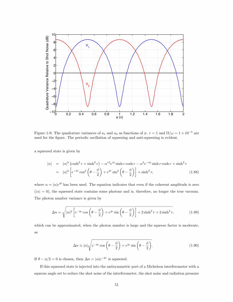
0 0.2 0.4 0.6 0.8 1 1.2 1.4 1.6 1.8 2−10

−8

−6

−4

−2

0

2

4

6

8

10

φ (π)

Qua

drat

ure

Varia

nce

Rela

tive

to S

hot N

oise

(dB)

V2

V1

Figure 1-9: The quadrature variances of a1 and a2 as functions of φ. r = 1 and Ω/ω = 1× 10−5 areused for the figure. The periodic oscillation of squeezing and anti-squeezing is evident.

a squeezed state is given by

〈n〉 = |α|2(

cosh2 r + sinh2 r)

− α∗2eiφ sinh r cosh r − α2e−iφ sinh r cosh r + sinh2 r

= |α|2[

e−2r cos2(

θ − φ

2

)

+ e2r sin2

(

θ − φ

2

)]

+ sinh2 r, (1.88)

where α = |α|eiθ has been used. The equation indicates that even if the coherent amplitude is zero

(|α| = 0), the squeezed state contains some photons and is, therefore, no longer the true vacuum.

The photon number variance is given by

∆n =

√

|α|2[

e−4r cos

(

θ − φ

2

)

+ e4r sin

(

θ − φ

2

)]

+ 2 sinh2 r + 2 sinh4 r, (1.89)

which can be approximated, when the photon number is large and the squeeze factor is moderate,

as

∆n % |α|

√

e−4r cos

(

θ − φ

2

)

+ e4r sin

(

θ − φ

2

)

. (1.90)

If θ − φ/2 = 0 is chosen, then ∆n = |α|e−2r is squeezed.

If this squeezed state is injected into the antisymmetric port of a Michelson interferometer with a

squeeze angle set to reduce the shot noise of the interferometer, the shot noise and radiation pressure

51

noise in Eqs. (1.61) and (1.66) become [10, 96, 82]

hshot(Ω) =1

L

√

hcλ

2πPine−r, hrad(Ω) =

1

mΩ2L

√

8πhPin

cλer. (1.91)

Since the shot noise and radiation pressure noise are the manifestations of the orthogonal quadra-

tures, if the squeeze factor r is constant, the shot noise and radiation pressure noise cannot be

reduced simultaneously. This issue will be discussed in Chap. 4.

1.5.3 Previous Experimental Efforts

Following the 1981 proposal of Caves [10], a handful of experimental efforts have realized the proof-

of-principle on the table-top scale at MHz frequencies. The pioneering experiment was performed

by Xiao et al. [11] using a Mach-Zehnder interferometer a few years after the first observation of

squeezed states by Slusher et al. in 1985 [12]. Later, squeezing-enhancement in table-top realizations

of Michelson interferometer configurations similar to those used in the current and future large-scale

GW detectors was demonstrated [13, 14]. McKenzie et al. [13] and Vahlbruch et al. [14] showed

squeezing-enhancement in power-recycled and dual-recycled Michelson interferometers on the table-

top scale at MHz frequencies, respectively.

However, these demonstrated techniques were not yet practical for the implementation of squeezing-

enhancement in large-scale GW detectors with suspended optics and complex readout and control

schemes such as LIGO and Advanced LIGO. This is the starting point of the thesis. The goal of the

thesis will be stated in the next section based on the previous experimental efforts.

1.6 The Goal of this Work

The goal of this thesis work is a detailed theoretical and experimental study of techniques necessary

for quantum-enhancement in laser-interferometric GW detectors. The work focuses on techniques

for the practical realization of quantum-enhancement in large-scale GW detectors with suspended

optics and readout and control schemes compatible with next generation GW detectors such as

Advanced LIGO.

Chap. 2 describes the theory of squeezed states including the generation, degradation, detec-

tion, and control of squeezed states using sub-threshold OPOs and homodyne detectors in the

two-photon formalism [19, 20]. Chap. 3 describes the experimental characterization of the tech-

niques discussed in Chap. 2 and presents experimental results. Chap. 4 discusses key require-

ments for quantum-enhanced GW detectors such as the frequency band, level, long-term stability,

and frequency-dependence of squeezing. Chap. 5 describes the theory of quantum-enhanced GW

detectors, especially in a quantum-enhanced signal-recycled Michelson interferometer (SRMI) con-

52

figuration, using a two-photon mathematical framework of quadrature field propagation. Chap. 6

describes the experimental demonstration of quantum-enhancement in a prototype GW detector in

the SRMI configuration using the techniques that have been developed throughout the period of

my Ph.D. work. Finally, Chap. 7 discusses possible future improvements and investigations toward

the actual implementation of the quantum-enhancement in long baseline laser-interferometric GW

detectors such as Advanced LIGO. The appendices show tables of constants, acronyms, and crystal

properties, a list of publications, and other work which may or may not be related to squeezing.

53

Chapter 2

Theory of Squeezed States

2.1 Overview

In 1927, Dirac proposed the wave-particle duality of light to account for interference phenomena and

yet explain the excitation of a specific atom located along a wavefront absorbing one photon of energy.

In this quantum theory of radiation, each mode of a radiation field can be understood by a quantized

simple harmonic oscillator [87, 86, 107]. An important consequence of the quantization of radiation

is the fluctuations associated with the zero-point energy or the so-called vacuum fluctuations. These

fluctuations have no classical analog and are responsible for many interesting phenomena in quantum

optics. The quantization of radiation fields is well described in Refs. [87, 86, 107, 89], and thus, not

fully derived in this thesis.

In classical physics, an electromagnetic field consists of waves with a well-defined amplitude and

phase. This is not the case when we treat the field quantum-mechanically. There are fluctuations

associated with both the amplitude and phase of the field. An electromagnetic field in a number

state |n〉 has a well-defined amplitude, but completely uncertain phase, while a field in a coherent

state has equal amount of uncertainties in the two quadratures that are conjugate to each other. The

uncertainties satisfy the Heisenberg uncertainty principle such that the product of the uncertainties in

the two quadrature field amplitudes is equal to or greater than half the magnitude of the expectation

value of the commutator of the variables as discussed in Sec. 1.4.2.

A squeezed state is a state in which fluctuations are reduced below the symmetric quantum

limit in one quadrature component. This is possible at the expense of increased fluctuations in the

canonically conjugate quadrature so that the Heisenberg uncertainty principle is not violated. A field

in a squeezed state has attractive applications in optical communication, photon detection, noise-

free amplification [108, 109], correlated twin-beam generation [110, 111], quantum teleportation

[112, 113], entanglement [114, 115], quantum imaging [116, 117, 118], quantum cryptography [119],

55

spectroscopic measurement [120, 121], polarization measurement [122], and precision measurement

[10, 13, 11, 122, 16, 15].

In this chapter, the concept of the quantization of radiation is used to explain states of light

such as coherent and squeezed states. In Sec. 2.2, the ball-on-stick picture is introduced to visu-

alize various quantum states. Furthermore, the generation, degradation, detection, and control of

squeezed states are theoretically introduced in Secs. 2.3, 2.5, 2.6, and 2.7, respectively, and then

experimentally demonstrated in the next chapter. Second-order nonlinear optical processes for the

generation of squeezed states are discussed in Sec. 2.4. In this thesis, we focus on the production

of squeezed states using sub-threshold optical parametric oscillators (OPOs) with second-order non-

linearity since the OPO-based squeezing has been the most commonly used technique (due to its

reliability and large squeezing level) for the generation of squeezed states. Other methods of squeez-

ing include Kerr squeezing [123, 124], quantum radiation pressure driven ponderomotive squeezing

[125, 126] and electromagnetically induced transparency (EIT) induced squeezing [127, 128], but

these techniques are not covered in this thesis.

It is important to note that throughout this chapter, we use the operator-linearization formalism

in which the linearization of operators is used to facilitate calculations of nonlinear equations of

motion. In the rest of the thesis, all equations are linear and the linearization of operators is not

used. Although the creation and annihilation operators are denoted δa† and δa in this chapter, the

amplitude and phase variances (∆a1 and ∆a2 in the time domain or Va1 and Va2 in the frequency

domain1) obtained from δa† and δa are essentially equivalent to ∆a1 and ∆a2 or Va1 and Va2

obtained from a† and a used in the other chapters. In other words, δa† and δa in this chapter are

equivalent to a† − a∗ and a − a in the other chapters.

2.2 States of Light

2.2.1 The Ball-on-Stick Picture

Overview

Various states of light and vacuum can be visually understood by use of the so-called ball-on-stick

picture of an electromagnetic field. This is analogous to the phasor diagram in classical physics where

the orthogonal axes are the real and imaginary parts of an electromagnetic field. The similarity is

that the stick represents the classical steady state coherent amplitude of the field whereas the

difference is that the ball on the stick represents noise that can be classical or quantum mechanical.

The noise ball can be regarded as a representation of the contour height of a probability distribution

1Va1 and Va2 will be defined later in this chapter.

56

ωt

a1

a2

u1

u2

∆a1

∆a2

ωt

a1

a2

u1

u2

∆a1

∆a2

u1

u2

∆a1?

∆a2?

Figure 2-1: Ball-on-stick pictures. Left : A coherent state with the minimum uncertainty. Center :A noisy state both classically and quantum-mechanically compared with a coherent state. Right : Avacuum state that is a coherent state of vacuum. In the left and center pictures, a1 and a2 [definedin Eqs. (1.46) and (1.47)] are the orthogonal amplitude and phase quadrature axes that rotate atthe field frequency ω with respect to the universal amplitude and phase quadrature axes with zerofrequency, denoted u1 and u2 respectively. In the right picture, the question marks in the vacuumquadrature variances reflect the fact that the amplitude and phase quadratures are undefined in thiscase.

function – the Wigner quasi-probability distribution function of an electromagnetic field given by [9]

WG(a1, a2) =2

π

1

∆a1∆a2exp

[

− (a1 − 2α1)2

2(∆a1)2− (a2 − 2α2)2

2(∆a2)2

]

, (2.1)

where we have only considered Gaussian statistics, and α1 = (α + α∗)/2 = |α| cos θ, and α2 =

(α − α∗)/(2i) = |α| sin θ. Wigner functions corresponding to a coherent state, a vacuum state,

amplitude and phase squeezed states are shown in Figs. 2-1 and 2-2. The Wigner function of any

Gaussian state can be completely defined by its standard deviation contour and a coherent amplitude

stick.

In this section, several common states such as a coherent state, a vacuum state, an amplitude

squeezed state of light, a phase squeezed state of light, and a squeezed state of vacuum are plotted

in the ball-on-stick picture to intuitively understand the various states. In Sec. 2.3.4, we will revisit

this ball-on-stick picture to visualize how an OPO generates a squeezed state.

The Coherent State

In quantum mechanics, a coherent state is a specific kind of quantum state of the quantum harmonic

oscillator whose dynamics most closely resemble the oscillating behavior of a classical harmonic

oscillator system. For instance, a coherent state describes the oscillating motion of a particle in a

quadratic potential well. In quantum optics, the coherent state |α〉 is defined in Eq. (1.54) [90, 89].

As shown in Fig. 2-1, the uncertainty on the stick is spread in all directions equally. A field in

a coherent state is a minimum-uncertainty state with equal uncertainties in the two quadrature

57

ωt

a1

a2

u1

u2

∆a1

∆a2

ωt

a1

a2

u1

u2

∆a1

∆a2

u1

u2

∆a1?

∆a2?

Figure 2-2: Ball-on-stick pictures. Left : An amplitude squeezed state compared with a coherentstate. Center : A phase squeezed state compared with a coherent state. Right : A squeezed state ofvacuum compared with a vacuum state. In the left and center pictures, a1 and a2 [defined in Eqs.(1.46) and (1.47)] are the orthogonal amplitude and phase quadrature axes that rotate at the fieldfrequency ω with respect to the universal amplitude and phase quadrature axes with zero frequency,denoted u1 and u2 respectively. In the right picture, the question marks in the vacuum quadraturevariances reflect the fact that the amplitude and phase quadratures are undefined in this case.

components so that ∆a1 = ∆a2 = 1.

The Noisy State

A state can be noisy both classically or quantum-mechanically. As shown in Fig. 2-1, the area of

the noise ball is always greater than unity and its shape can be both elliptic and circular so that

∆a1 > 1 and ∆a2 > 1 simultaneously, but its semiminor axis can never be less than the radius of

the noise ball of the coherent state.

The Vacuum State

A vacuum state is a coherent state of light with no coherent steady state amplitude and the minimum

uncertainty. Since the vacuum has no coherent amplitude, its amplitude and phase quadrature axes

are undefined. This means it is meaningless to discuss amplitude and phase quadratures since they

are nonexistent unless it beats with a coherent field. To reflect this, we use a question mark in our

notation, so that ∆a1? and ∆a2? denote the undefined quadrature variances, which are shown in

Fig. 2-1.

The Amplitude Squeezed State of Light

An amplitude (coherent) squeezed state of light is obtained when a coherent state of light is squeezed

in the amplitude quadrature. The semiminor axis of the squeezed noise ball is less than the radius

of the noise ball of the coherent state. However, the area of the noise ellipse must remain equal to or

greater than unity so that the Heisenberg uncertainty principle is not violated. The state is shown

58

in Fig. 2-2. In this case, ∆a1 < 1 and ∆a2 > 1, but ∆a1∆a2 = 1 (in the case of perfect squeezing).

The Phase Squeezed State of Light

A phase (coherent) squeezed state of light is obtained when a coherent state of light is squeezed in

the phase quadrature. Similar to the amplitude squeezed state of light, the area of the ellipse ball

must be equal to or greater than unity. The state is shown in Fig. 2-2. In this case, ∆a1 > 1 and

∆a2 < 1, but ∆a1∆a2 = 1 (in the case of perfect squeezing).

The Squeezed State of Vacuum

A squeezed state of vacuum is obtained when a vacuum state is squeezed. Just like a vacuum state, a

squeezed vacuum state has no coherent amplitude, and therefore, its quadrature axes are undefined.

The quadrature axes can be defined only when the state interacts with a coherent field. However,

this interaction converts the squeezed vacuum state to a squeezed state of light, and therefore, it is

no longer a squeezed state of vacuum. The state is shown in Fig. 2-2. Here, similar to the amplitude

or phase squeezed state of light, ∆a1? < 1 and ∆a2? > 1, but ∆a1?∆a2? = 1 (in the case of perfect

squeezing).

2.2.2 Equivalence of Squeezed Light and Squeezed Vacuum

A squeezed state of light or a squeezed state of vacuum are often shortened to be squeezed light or

squeezed vacuum, respectively. In addition, in the previous section, a squeezed state of light and

a squeezed state of vacuum are separately described. However, they are essentially identical since

they are vacuum fluctuations on top of the coherent stick that are squeezed, not light. The light

often refers to the coherent amplitude or the stick.

2.3 Generation of Squeezed States

2.3.1 Introduction

In classical optics, the sideband model is widely used to visually understand amplitude and phase

modulation. Amplitude- or phase-modulated fields can be considered as the sum of correlated

coherent sidebands relative to the frequency of a carrier field. Likewise, in quantum optics, the

coherent state can be the sum of uncorrelated quantum sidebands which are a pair of creation

and annihilation operators in the ground state of a simple harmonic oscillator, hω/2, at every

frequency and beat against the carrier field. For a coherent state, all quantum sidebands have

random amplitude and phase and therefore, the result is broadband white noise or shot noise in

both the amplitude and phase quadratures. In other words, quantum noise is distributed equally

59

(randomly) in both the amplitude and phase quadratures. A squeezed state can be considered as

the sum of correlated quantum sidebands relative to the carrier frequency, just as amplitude- and

phase-modulated fields are the sum of correlated coherent sidebands relative to the carrier frequency.

At frequencies where squeezing occurs, the upper and lower quantum sidebands around the carrier

frequency become correlated or synchronized with each other. This quantum sideband correlation

picture can be understood most rigorously by the two-photon formalism [19, 20]. In the formalism,

a squeezed state is obtained by acting with displacement operators on a vacuum state followed by a

two-photon squeeze operator, as described in Sec. 1.5.2.

Among many methods of generating squeezed states in practice, optical parametric oscillation

(OPO)2 has been one of the most common techniques that do the operation described above since

it was first observed by Wu et al. in 1986 [129]. An OPO is a two-photon correlator that correlates

upper and lower quantum sidebands centered around the frequency of a carrier field or half the

frequency of an energetic pump field. Squeezing is basically equivalent to the sum of correlated

quantum sidebands, and thus, must be treated using the two-photon formalism. The generation of

squeezed states is described in many textbooks, often using degenerate OPO (DOPO) as a model

of squeezing-production. However, this sometimes leads to the misunderstanding of squeezing. In

the following sections, the production of squeezed states using nondegenerate OPO (NDOPO) is

introduced to properly understand the origin and physical meaning of squeezed states. The proper

understanding of squeezed states in the two-photon formalism is necessary to understand the injec-

tion of squeezed states into laser-interferometric gravitational wave (GW) detectors since they are

essentially two-photon devices and squeezed states are two-photon correlated states produced by

OPOs as two-photon correlators.

2.3.2 Quantization of Quadrature Field Amplitudes in Two-Photon For-

malism

Consider a carrier field at ω and a pair of sidebands relative to the carrier at ω±Ω. The upper and

lower sidebands are the so-called signal and idler of the carrier field [130]. The total electric field is

given by integrating the signal and idler fields over all positive and negative frequencies around zero

frequency,

E(t) =

∫

dΩ[

E(ω + Ω)eiΩt + E(ω − Ω)e−iΩt]

eiωt

+

∫

dΩ[

E†(ω + Ω)e−iΩt + E†(ω − Ω)eiΩt]

e−iωt. (2.2)

2Throughout the thesis, OPO stands for both optical parametric oscillation and optical parametric oscillatoralthough this abbreviation might be confusing.

60

Using the standard operator expressions, E(ω + Ω) and E(ω − Ω) can be written as

E(ω + Ω) = E√

ω + Ω

2ωas(ω + Ω), E(ω − Ω) = E

√

ω − Ω

2ωai(ω − Ω), (2.3)

where

E =

√

hω

2πε0cA, (2.4)

and the subscripts (s and i) stand for the signal and idler. Here h is Planck’s constant, ε0 is the

permittivity of vacuum, c is the speed of light in vacuum, and A is the effective cross section of the

field. It is important to note that the coefficients,√

(ω ± Ω) /2, are necessary for the correct energy

eigenvalues, h (ω ± Ω). As Ω → 0, both equations reduce to the field equations in the degenerate

case. as and ai satisfy the commutation relations,

[

as, a†s′

]

% 2πδ(Ω − Ω′

), (2.5)[

ai, a†i′

]

% 2πδ(Ω − Ω′

). (2.6)

Frequency

Re(E)

ω+Ωω-Ω

-ω+Ω-ω-Ω

-ω

ωCarrier

Carrier

as

ai†

ai

as†

Im(E)

Figure 2-3: The signal and idler fields relative to the frequency of a carrier field. The signal andidler fields can be classical or quantum-mechanical.

Eq. (2.2) can be rewritten in terms of two orthogonal quadrature electric fields as

E(t) = E1(t) cosωt + E2(t) sinωt

=

∫

dΩ[

E1(Ω)eiΩt + E†1(Ω)e−iΩt

]

cosωt +

∫

dΩ[

E2(Ω)eiΩt + E†2(Ω)e−iΩt

]

sinωt, (2.7)

61

where

E1(Ω) = E(ω + Ω) + E†(ω − Ω), (2.8)

E2(Ω) = −i[

E(ω + Ω) − E†(ω − Ω)]

. (2.9)

Defining the amplitude and phase quadrature fields by

a1(Ω) =

√

ω + Ω

ωas(ω + Ω) +

√

ω − Ω

ωa†

i (ω − Ω) Amplitude Quadrature, (2.10)

a2(Ω) = −i

[

√

ω + Ω

ωas(ω + Ω) −

√

ω − Ω

ωa†

i (ω − Ω)

]

Phase Quadrature, (2.11)

Eqs. (2.8) and (2.9) can be rewritten as

E1(Ω) =E√2a1(Ω), (2.12)

E2(Ω) =E√2a2(Ω). (2.13)

Hence, the electric field in Eq. (2.7) is given in terms of a1 and a2 by

E(t) =E√2

∫

dΩ (a1 cosωt + a2 sinωt) eiΩt +E√2

∫

dΩ(a†1 cosωt + a†

2 sinωt)e−iΩt

=E√2

[(∫

a1eiΩtdΩ

)

cosωt +

(∫

a2eiΩtdΩ

)

sinωt

]

+E√2

[(∫

a†1e

−iΩtdΩ

)

cosωt +

(∫

a†2e

−iΩtdΩ

)

sinωt

]

, (2.14)

which clearly indicates that a1 and a2 are the orthogonal quadratures. The second component is

often ignored since it is the complex conjugate of the first component.

As Ω → 0, Eqs. (2.10) and (2.11) reduce to the amplitude and phase quadrature operators in

the degenerate case,

a1 = a + a†, (2.15)

a2 = −i(

a − a†) . (2.16)

In most cases, Ω + ω. For example, for an optical field at λ = 1064 nm, ω/(2π) % 1015 Hz. The

frequency of interest Ω is typically on the order of MHz or lower, and therefore, the coefficients√

1 ± Ω/ω in Eqs. (2.10) and (2.11) are often reduced to unity3.

3However, this simplification often leads to the misunderstanding of the commutation relations in Eqs. (2.5) and(2.6), and then Eqs. (2.15) and (2.16) are incorrectly used as if the carrier was at zero frequency.

62

2.3.3 Generation of Squeezed States in Optical Parametric Oscillation

Overview

We now turn to the discussion of how to generate squeezed states in practice or more specifically how

to do the two-photon squeeze operation described in Sec. 1.5.2. Although there are many methods

of generating squeezed states, we focus on OPO with second-order nonlinearity, which is one of the

most common and reliable methods of squeezing. In this section, a model of optical cavities with

second-order nonlinear media in the form of quantum Langevin equations of motion is introduced.

Equations of Motion for Optical Cavities with Second-Order Nonlinear Media

As shown in Fig. 2-4, consider that three different fields as(ω + Ω), ai(ω − Ω), and b(2ω) enter

a system that involves a second-order nonlinear interaction, the most general Hamiltonian for the

system is given by [131, 132, 133]

H = Hsys + Hu + Hint, (2.17)

where Hsys is the Hamiltonian for the internal modes in the closed system (cavity) given by

Hsys = h(ω + Ω)a†sas + h(ω − Ω)a†

iai + h(2ω)b†b, (2.18)

Hu is the Hamiltonian for the open system that interacts with the universe given by

Hu = ih

∫ ∞

−∞

[

√

2γus

(

u†sas − a†

sus

)

+√

2γui

(

u†i ai − a†

i ui

)

+√

2γub

(

u†b b − b†ub

)]

dΩ, (2.19)

and Hint is the Hamiltonian for the nonlinear interaction given by

Hint =1

2ihε

(

a†sa

†i b − asaib

†)

. (2.20)

Here as and ai are signal and idler fields with respect to the fundamental frequency ω, b is a

second-harmonic field at the second-harmonic frequency 2ω, ε is the second-order nonlinear coupling

constant, and us, ui, and ub are the external modes coupled with the associated internal modes. The

origin of the second-order nonlinearity will be described in Sec. 2.4.

Using the quantum Langevin approach [131, 132], the Heisenberg equations of motion for the

intra-cavity fields [as(ω + Ω), ai(ω −Ω), b(2ω)] are respectively given in terms of all the input fields

63

εBin

δvsl δvb

l

δvsout δvb

out

γsout γb

out

as

b

γsin γb

in

γsl γb

l

δvil

γil

ai

γiout

δviout

γiin

Aiin As

out BoutAioutAs

in

Figure 2-4: A model of an optical cavity with a second-order nonlinear medium with three inputfields [Ain

s (ω + Ω), Aini (ω −Ω), Bin(2ω)], three intra-cavity fields [as(ω + Ω), ai(ω −Ω), b(2ω)], three

output fields [Aouts (ω + Ω), Aout

i (ω−Ω), Bout(2ω)], vacuum fields associated with the correspondingoutput coupling losses [δvout

s (ω+Ω), δvouti (ω−Ω), δvout

b (2ω)], and vacuum fields associated with thecorresponding intra-cavity losses [δvl

s(ω + Ω), δvli(ω − Ω), δvl

b(2ω)].

and cross-couplings with them by [131, 132, 133]

as =1

ih[as,Hsys + Hint] − γtot

s as +√

2γins Ain

s ei(ω+Ω)t +√

2γouts δvout

s +√

2γlsδv

ls, (2.21)

ai =1

ih[ai,Hsys + Hint] − γtot

i ai +√

2γini Ain

i ei(ω−Ω)t +√

2γouti δvout

i +√

2γliδv

li, (2.22)

b =1

ih[b,Hsys + Hint] − γtot

b b +√

2γinb Binei(2ω)t +

√

2γoutb δvout

b +√

2γlbδv

lb. (2.23)

Transforming into the rotating frame of each field with

as → e−i(ω+Ω)tas, Ains → e−i(ω+Ω)tAin

s , (2.24)

ai → e−i(ω−Ω)tai, Aini → e−i(ω−Ω)tAin

i , (2.25)

b → e−i(2ω)tb, Bin → e−i(2ω)tBin, (2.26)

we simplify Eqs. (2.21), (2.22), and (2.23) to be [134]

as = −(

γtots − iωd

s

)

as +1

2εa†

i b +√

2γins Ain

s +√

2γouts δvout

s +√

2γlsδv

ls, (2.27)

ai = −(

γtoti − iωd

i

)

ai +1

2εa†

sb +√

2γini Ain

i +√

2γouti δvout

i +√

2γliδv

li, (2.28)

b = −(

γtotb − iωd

b

)

b − 1

2εasai +

√

2γinb Bin +

√

2γoutb δvout

b +√

2γlbδv

lb, (2.29)

where as, ai, and b are intra-cavity fields, Ains , Ain

i , and Bin are input fields, δvouts , δvout

i , and δvoutb

64

are output coupling vacuum fields, δvls, δvl

i, and δvlb are fields associated with intra-cavity losses

characterized by the associated cavity decay constants γ’s respectively, and γtots , γtot

i , and γtotb are

the sum of all the decay constants in each mode so that γtots = γin

s +γouts +γl

s, γtoti = γin

i +γouti +γl

i,

and γtotb = γin

b + γoutb + γl

b. Here ωds , ωd

i , and ωdb are the cavity detunings given by ωd

s = ω + Ω− ωcs,

ωdi = ω − Ω − ωc

i , and ωdb = 2ω − ωc

b , where ωcs, ωc

i , and ωcb are the cavity resonance frequencies

in the corresponding modes. We have assumed that the nonlinear coupling constant ε which is

usually temperature dependent is optimized and is therefore real4. Throughout the rest of the

chapter, we will assume that the cavity detunings and the frequency of interest Ω are much smaller

than the associated decay rates and therefore, we will ignore them, such that γtots − iωd

s % γtots ,

γtoti − iωd

i % γtoti , and γtot

b − iωdb % γtot

b . This general system of equations accounts for all second-

order nonlinear interactions including DOPO and NDOPO and second-harmonic generation (SHG).

Which interaction to choose depends on the phase-matching condition, which will be described in

Sec. 2.4.4.

Quadrature Field Amplitudes

The most common method of generating the analytic form of squeezed quadrature variances is to

expand the operators about their steady state values and then linearize the resulting expressions

to first-order in the fluctuation terms [136]. To linearize the equations of motion, we make the

substitution for the annihilation and creation operators for as and a†s,

as = as + δas, a†s = a∗

s + δa†s (2.30)

(similarly for ai, b, Ains , Ain

i , and Bin). as is the complex expectation value 〈as〉 (so that as = 〈as〉)

and δas is the operator for the fluctuations in as so that 〈δas〉 = 0. δAins , δAin†

s , δAini , and δAin†

i

satisfy the commutation relations,

[

Ains , Ain†

s′

]

= 2πδ(Ω − Ω′

), (2.31)[

Aini , Ain†

i′

]

= 2πδ(Ω − Ω′

), (2.32)

and all others vanish.

We then separate Eqs. (2.27), (2.28), and (2.29) into the time-dependent fluctuation component

and time-independent coherent amplitude component. The coherent components of the equations

4The nonlinear coupling constant ε is a function of the phase mismatch parameter ∆k, so that ε =κ0zei∆kz/2sinc(∆kz/2), where κ0 is a constant and z is the nonlinear interaction length. The dependence of ∆kon the temperature of the nonlinear medium will be described in Sec. 2.4. Refs. [134, 135] describe the cases of cavitydetunings and complex nonlinear coupling constants.

65

are given by

0 = −γtots as +

1

2εa∗

i b +√

2γins Ain

s , (2.33)

0 = −γtoti ai +

1

2εa∗

s b +√

2γini Ain

i , (2.34)

0 = −γtotb b − 1

2εasai +

√

2γinb Bin. (2.35)

Assuming that the pump field is undepleted, as is often the case, (εasai + γtotb b), Eq. (2.35) reduces

to

0 % −γtotb b +

√

2γinb Bin. (2.36)

Solving for the intra-cavity states yields

as

a∗i

=

γtots − 1

2εb

− 12εb

∗ γtoti

−1

√

2γins Ain

s√

2γini Ain∗

i

, (2.37)

where b =√

2γinb Bin/γtot

b . The fluctuation components of Eqs. (2.27), (2.28), and (2.29) are

similarly given by

δas = −γtots δas +

1

2εa∗

i δb +1

2εbδa†

i +√

2γins δAin

s +√

2γouts δvout

s +√

2γlsδv

ls, (2.38)

δai = −γtoti δai +

1

2εa∗

sδb +1

2εbδa†

s +√

2γini δAin

i +√

2γouti δvout

i +√

2γliδv

li, (2.39)

δb = −γtotb δb − 1

2εasδai −

1

2εaiδas +

√

2γinb δBin +

√

2γoutb δvout

b +√

2γlbδv

lb. (2.40)

In terms of frequency components defined in Eq. (1.60), Eqs. (2.38), (2.39), and (2.40) can be

rewritten in a compact form,

iΩxc = Mcxc + Minxin + Moutvout + Mlvl, (2.41)

where the field vectors are defined by

xc ≡

δas

δa†s

δai

δa†i

δb

δb†

, xin ≡

δAins

δAin†s

δAini

δAin†i

δBin

δBin†

, vout ≡

δvouts

δvout†s

δvouti

δvout†i

δvoutb

δvout†b

, vl ≡

δvls

δvl†s

δvli

δvl†i

δvlb

δvl†b

, (2.42)

66

and the coupling matrices are defined by

Mc ≡

−γtots 0 0 1

2εb12εa

∗i 0

0 −γtots

12εb

∗ 0 0 12εai

0 12εb −γtot

i 0 12εa

∗s 0

12εb

∗ 0 0 −γtoti 0 1

2εas

− 12εai 0 − 1

2εas 0 −γtotb 0

0 − 12εa

∗i 0 − 1

2εa∗s 0 −γtot

b

, (2.43)

Min ≡ diag

(

√

2γins ,

√

2γins ,

√

2γini ,

√

2γini ,

√

2γinb ,

√

2γinb

)

, (2.44)

Mout ≡ diag

(

√

2γins ,

√

2γouts ,

√

2γouti ,

√

2γouti ,

√

2γoutb ,

√

2γoutb

)

, (2.45)

Ml ≡ diag

(

√

2γls,√

2γls,√

2γli,√

2γli,√

2γlb,√

2γlb

)

. (2.46)

Thus, the cavity field vector is found to be

xc = (iΩI − Mc)−1 (Minxin + Moutvout + Mlvl) , (2.47)

where I ≡ diag(1, 1, 1, 1, 1, 1) is the identity matrix. The output field vector defined by

xout ≡(

δAouts , δAout†

s , δAouti , δAout†

i , δBout, δBout†)T

, (2.48)

where T is the transpose, is thus found to be [131, 132]

xout = Moutxc − vout

= Mout (iΩI − Mc)−1

Minxin +[

Mout (iΩI − Mc)−1

Mout − I]

vout

+Mout (iΩI − Mc)−1

Mlvl, (2.49)

which indicates that the output field xout is determined by the input field xin and the vacuum fields

vout and vl with the associated transfer functions Mout (iΩI − Mc)−1

Min, Mout (iΩI − Mc)−1

Mout−

I, and Mout (iΩI − Mc)−1

Ml.

Following the amplitude and phase quadrature fields in Eqs. (2.10) and (2.11), the quadrature

field amplitudes of the input field (δAin1 and Ain

2 ) are defined in the frequency domain (the same as

in the time domain) by

δAin1 (Ω) ≡

√

ω + Ω

ωδAin

s (ω + Ω) +

√

ω − Ω

ωδAin†

i (ω − Ω), (2.50)

δAin2 (Ω) ≡ −i

[

√

ω + Ω

ωδAin

s (ω + Ω) −√

ω − Ω

ωδAin†

i (ω − Ω)

]

, (2.51)

67

(similarly for δvout1 , δvout

2 , δvl1, δv

l2, δA

out1 , and δAout

2 ). Correspondingly, Eqs. (2.31) and (2.32) imply

the commutation relations for the quadrature field amplitudes in the frequency domain,

[

δAin1 (Ω), δAin†

2 (Ω′

)]

= −[

δAin2 (Ω), δAin†

1 (Ω′

)]

= −2iδ(Ω − Ω′

), (2.52)

(similarly for δvout1 , δvout

2 , δvl1, and δvl

2) and all others vanish.

For simplicity, we assume the frequency of interest is much smaller than the linewidth of the

OPO cavity at each wavelength such that Ω + γjs , γj

i for j = in, out, and l. It is also reasonable

to assume |a|δb + |b|δa in the case of the undepleted pump since |a| +| b| and the fluctuations in

the pump and seed fields are on the same order. In addition, we assume γjs % γj

i for j = in, out,

and l and thus drop the subscript by denoting γja ≡ γj

s % γji for j = in, out, and l. Under these

assumptions, the quadrature field amplitudes of the output field are found to be

δAout1 (Ω) =

√

2γina

[

C +D

2

(

√

ω + Ω

ω − Ωeiφ +

√

ω − Ω

ω + Ωe−iφ

)]

δAin1 (Ω)

+

√

2γouta

[

C +D

2

(

√

ω + Ω

ω − Ωeiφ +

√

ω − Ω

ω + Ωe−iφ

)]

− 1

δvout1 (Ω)

+√

2γla

[

C +D

2

(

√

ω + Ω

ω − Ωeiφ +

√

ω − Ω

ω + Ωe−iφ

)]

δvl1(Ω)

−i√

2γina

D

2

(

√

ω + Ω

ω − Ωeiφ −

√

ω − Ω

ω + Ωe−iφ

)

δAin2 (Ω)

−i√

2γouta

D

2

(

√

ω + Ω

ω − Ωeiφ −

√

ω − Ω

ω + Ωe−iφ

)

δvout2 (Ω)

−i√

2γlaD

2

(

√

ω + Ω

ω − Ωeiφ −

√

ω − Ω

ω + Ωe−iφ

)

δvl2(Ω), (2.53)

δAout2 (Ω) =

√

2γina

[

C − D

2

(

√

ω + Ω

ω − Ωeiφ +

√

ω − Ω

ω + Ωe−iφ

)]

δAin2 (Ω)

+

√

2γouta

[

C − D

2

(

√

ω + Ω

ω − Ωeiφ +

√

ω − Ω

ω + Ωe−iφ

)]

− 1

δvout2 (Ω)

+√

2γla

[

C − D

2

(

√

ω + Ω

ω − Ωeiφ +

√

ω − Ω

ω + Ωe−iφ

)]

δvl2(Ω)

−i√

2γina

D

2

(

√

ω + Ω

ω − Ωeiφ −

√

ω − Ω

ω + Ωe−iφ

)

δAin1 (Ω)

−i√

2γouta

D

2

(

√

ω + Ω

ω − Ωeiφ −

√

ω − Ω

ω + Ωe−iφ

)

δvout1 (Ω)

−i√

2γlaD

2

(

√

ω + Ω

ω − Ωeiφ −

√

ω − Ω

ω + Ωe−iφ

)

δvl1(Ω), (2.54)

where φ is the phase of the pump field (or equivalently the squeeze angle) such that Bin = |Bin|eiφ

68

and

C ≡√

2γouta

γtota

1

1 − x2, D ≡ −

√

2γouta

γtota

x

1 − x2. (2.55)

Here x is the coupling of the nonlinear interaction normalized to the OPO threshold given by

x =ε|b|

2γtota

(2.56)

and should be less than unity not to lase.

Reduction to the Degenerate Case

In most cases, Ω + ω, and therefore, the quadrature field amplitudes in NDOPO are approximately

equal to those in DOPO. In the DOPO limit (Ω/ω → 0), the two modes coalesce into a single mode

at frequency ω, such that

√

ω + Ω

ω − Ωeiφ +

√

ω − Ω

ω + Ωe−iφ → 2 cosφ, (2.57)

√

ω + Ω

ω − Ωeiφ −

√

ω − Ω

ω + Ωe−iφ → 2i sinφ. (2.58)

The quadrature field amplitudes, δAout1 (Ω) and δAout

2 (Ω), then reduce to

δAout1 (Ω) =

[

2√

γina γout

a

γtota

1 − x cosφ

1 − x2

]

δAin1 (Ω) +

[

2γouta

γtota

1 − x cosφ

1 − x2− 1

]

δvout1 (Ω)

+

[

2√

γlaγ

outa

γtota

1 − x cosφ

1 − x2

]

δvl1(Ω) −

[

2√

γina γout

a

γtota

x sinφ

1 − x2

]

δAin2 (Ω)

−[

2γouta

γtota

x sinφ

1 − x2

]

δvout2 (Ω) −

[

2√

γlaγ

outa

γtota

x sinφ

1 − x2

]

δvl2(Ω), (2.59)

δAout2 (Ω) =

[

2√

γina γout

a

γtota

1 + x cosφ

1 − x2

]

δAin2 (Ω) +

[

2γouta

γtota

1 + x cosφ

1 − x2− 1

]

δvout2 (Ω)

+

[

2√

γlaγ

outa

γtota

1 + x cosφ

1 − x2

]

δvl2(Ω) −

[

2√

γina γout

a

γtota

x sinφ

1 − x2

]

δAin1 (Ω)

−[

2γouta

γtota

x sinφ

1 − x2

]

δvout1 (Ω) −

[

2√

γlaγ

outa

γtota

x sinφ

1 − x2

]

δvl1(Ω), (2.60)

which agree with the quadrature field amplitudes in the degenerate case [131].

Quadrature Variances

In squeezing experiments, spectrum analyzers are often used to obtain squeezed and anti-squeezed

quadrature variances after measuring squeezed fields with photodetectors. The detection of squeezed

69

states will be described in Sec. 2.6. As defined by Eq. (1.44), the normalized quadrature variances

of the output field [V outA1

(Ω) and V outA2

(Ω)] in the frequency domain for quadrature fields [δAout1 and

δAout2 ] are given by [131, 137]

V outA1

(Ω) ≡⟨

∣

∣

∣Aout

1 (Ω) −⟨

Aout1

⟩∣

∣

∣

2⟩

=

⟨

∣

∣

∣δAout

1 (Ω)∣

∣

∣

2⟩

Amplitude Variance, (2.61)

V outA2

(Ω) ≡⟨

∣

∣

∣Aout

2 (Ω) −⟨

Aout2

⟩∣

∣

∣

2⟩

=

⟨

∣

∣

∣δAout

2 (Ω)∣

∣

∣

2⟩

Phase Variance, (2.62)

(similarly for all the input modes). From Eqs. (2.59) and (2.60), the amplitude and phase quadrature

variances of the output field are, respectively, found to be

V outA1

(Ω) =

[

2√

γina γout

a

γtota

1 − x cosφ

1 − x2

]2

V inA1

(Ω) +

[

2γouta

γtota

1 − x cosφ

1 − x2− 1

]2

V outv1

(Ω)

+

[

2√

γlaγ

outa

γtota

1 − x cosφ

1 − x2

]2

V lv1

(Ω) +

[

2√

γina γout

a

γtota

x sinφ

1 − x2

]2

V inA2

(Ω)

+

[

2γouta

γtota

x sinφ

1 − x2

]2

V outv2

(Ω) +

[

2√

γlaγ

outa

γtota

x sinφ

1 − x2

]2

V lv2

(Ω), (2.63)

V outA2

(Ω) =

[

2√

γina γout

a

γtota

1 + x cosφ

1 − x2

]2

V inA2

(Ω) +

[

2γouta

γtota

1 + x cosφ

1 − x2− 1

]2

V outv2

(Ω)

+

[

2√

γlaγ

outa

γtota

1 + x cosφ

1 − x2

]2

V lv2

(Ω) +

[

2√

γina γout

a

γtota

x sinφ

1 − x2

]2

V inA1

(Ω)

+

[

2γouta

γtota

x sinφ

1 − x2

]2

V outv1

(Ω) +

[

2√

γlaγ

outa

γtota

x sinφ

1 − x2

]2

V lv1

(Ω), (2.64)

Since all the input vacuum modes are in the coherent state, from Eq. (1.50), V (Ω) = 1 for all the

vacuum modes, such that Eqs. (2.63) and (2.64) become

V outA1

(Ω) =

[

2√

γina γout

a

γtota

1 − x cosφ

1 − x2

]2

V inA1

(Ω) +

[

2√

γina γout

a

γtota

x sinφ

1 − x2

]2

V inA2

(Ω)

+

[

2γouta

γtota

1 − x cosφ

1 − x2− 1

]2

+

[

2γouta

γtota

x sinφ

1 − x2

]2

+

[

2√

γlaγ

outa

γtota

1 − x cosφ

1 − x2

]2

+

[

2√

γlaγ

outa

γtota

x sinφ

1 − x2

]2

, (2.65)

V outA2

(Ω) =

[

2√

γina γout

a

γtota

1 + x cosφ

1 − x2

]2

V inA2

(Ω) +

[

2√

γina γout

a

γtota

x sinφ

1 − x2

]2

V inA1

(Ω)

+

[

2γouta

γtota

1 + x cosφ

1 − x2− 1

]2

+

[

2γouta

γtota

x sinφ

1 − x2

]2

+

[

2√

γlaγ

outa

γtota

1 + x cosφ

1 − x2

]2

+

[

2√

γlaγ

outa

γtota

x sinφ

1 − x2

]2

, (2.66)

70

and therefore, the quadrature variances of the output field are linear functions of the quadrature

variances of the input or seed field, V inA1

(Ω) and V inA2

(Ω). Since all the coefficients of the input

quadrature variances are frequency-independent, the frequency-dependency of the output quadrature

variances is completely determined by the quadrature variances of the input field at low frequencies.

At high frequencies, although we have omitted the high frequency cutoff determined by the linewidth

of the OPO cavity since we have assumed Ω + γina , γout

a , γla, it appears in the 1 − x2 denominator

and therefore, all the coefficients containing 1− x2 in the denominators decay to zero at frequencies

where Ω > γina , γout

a , γla.

In the case of generating a squeezed state of light, the seed field is a bright field which is

typically noisy at frequencies below 1 MHz due to its classical laser noise and therefore is not shot-

noise-limited. In other words, V inA1

(Ω) and V inA2

(Ω) are much greater than unity at low frequencies

including the GW detection band. On the other hand, in the case of generating a squeezed state of

vacuum, the seed field is a vacuum field in the coherent state, and therefore, V inA1

(Ω) = V inA2

(Ω) = 1

at all frequencies, such that Eqs. (2.65) and (2.66) become

V outA1

(Ω) = 1 + 4ηout2x2 − x cosφ− x2 cosφ

(1 − x2)2, (2.67)

V outA2

(Ω) = 1 + 4ηout2x2 + x cosφ + x2 cosφ

(1 − x2)2, (2.68)

where ηout ≡ γouta /γtot

a is the escape efficiency. As defined in Sec. 1.5.2, φ is the squeeze angle that

determines which quadrature to squeeze. The squeezed and anti-squeezed quadrature variances are

found from Eqs. (2.67) and (2.68) to be

V outA1

∣

∣

∣

φ=0= V out

A2

∣

∣

∣

φ=π= 1 − 4ηout

x

(1 + x)2, (2.69)

V outA2

∣

∣

∣

φ=0= V out

A1

∣

∣

∣

φ=π= 1 + 4ηout

x

(1 − x)2. (2.70)

Therefore, the generated level of squeezing5 is completely determined by the escape efficiency ηout

and the nonlinear coupling efficiency x. These equations are often seen in many publications [138,

139, 140, 141, 18, 142, 143]. Again, it is important to note that they are in the limiting case we

have assumed. Throughout the rest of the thesis, we will continue to assume that Ω + ω so that

any term that contains Ω/ω will be ignored.

2.3.4 The Ball-on-Stick Picture Revisited

In the previous section, the generation of squeezed states in an OPO has been mathematically

described using the two-photon formalism. Although the two-photon description of the squeeze

5The detected level of squeezing is always lower than the generated level of squeezing since the detection efficiencyof a detector has to be taken into account.

71

state production is rigorous and precise, its mathematical complexity does not appeal to an intuitive

understanding. In this section, to facilitate the two-photon description of the squeezing generation,

we revisit the ball-on-stick picture to visualize how the OPO produces a squeezed state.

(c)

(b)(a)

εω+Ω

ω+Ωω-Ω

OPO

SignalIdler

SeedCorrelated

Pump2ω

Pump2ω

ω+Ω

ω-Ω

Signal

Idler

ωtu1

u2

Signal

Idler

+Ω-Ω

ωtu1

u2

Signal

Idler

Figure 2-5: The production of a squeezed state in the ball-on-stick picture: (a) difference frequencygeneration in nondegenerate optical parametric oscillation, (b) energy level diagram for the interac-tion, (c) a phase-squeezed state created by the sum of correlated signal and idler photons.

Fig. 2-5 shows the production of a squeezed state in the ball-on-stick picture. Suppose that two

coherent photons at ω + Ω are injected as a seed into a second-order nonlinear medium ε, and then,

an idler photon at ω−Ω is created due to the difference frequency generation in the NDOPO excited

by one of the seed photons at ω + Ω in the presence of a pump photon at 2ω, leaving the other seed

photon (signal) transmitted, as shown in Fig. 2-5(a). The transmitted signal and generated idler

photons are, therefore, correlated. The energy level diagram for the interaction is shown in Fig.

2-5(b).

Suppose that the signal and idler photons beat with a coherent field (carrier) at ω. Assuming

that the signal and idler photons have an equal amplitude for simplicity6, they rotate with respect

6The equal amplitude is assumed since we want modulation to occur only along the amplitude or phase axis ofthe carrier. If the signal and idler amplitudes are not equal, the modulation axis is tilted relative to the amplitude orphase axis of the carrier, but does not lose generality.

72

to the carrier axis at ω counterclockwise at +Ω and clockwise at −Ω respectively in the ball-on-stick

picture as shown in Fig. 2-5(c). The sum of these signal and idler vectors travels only along the

amplitude axis of the carrier, modulating the amplitude of the carrier at Ω. This is analogous to

classical amplitude modulation (AM). If the idler has an initial phase of π so that the signal rotates

counterclockwise at Ωt and the idler rotates clockwise at Ωt + π, the sum of these signal and idler

vectors travels only along the phase axis of the carrier, modulating the phase (frequency) of the

carrier at Ω. This is analogous to classical frequency modulation (FM).

Squeezing is just like AM and FM, but quantum-mechanically. Assume that two vacuum photons

(vacuum fluctuations) at ω + Ω enter the second-order nonlinear medium. Due to the difference

frequency generation in the NDOPO excited by the vacuum photons at ω + Ω, the transmitted

signal and generated idler vacuum photons at ω±Ω are correlated. They rotate with respect to the

carrier just like the coherent signal and idler photons in the ball-on-stick picture. Assuming that the

initial phase difference between the two is 0 or π, the sum of these signal and idler vacuum photons

travels only along either the amplitude or phase axis of the carrier, yielding quantum-mechanical

AM and FM. In practice, when a number of photons enter the OPO, not all of them interact with

the pump fields, and thus, the signal-idler photon correlations are not perfect. Then, the sum of all

the vectors becomes an ellipse – or a squeezed state. The probabilistic distribution of the correlated

photons is given by the Wigner quasi-probability distribution function in Eq. (2.1). Fig. 2-6 shows

the Wigner functions of a coherent state and amplitude and phase squeezed states.

Figure 2-6: The Wigner functions given by Eq. (2.1) for three common states. Left : A coherent state.Center : An amplitude-squeezed state with ∆a1 = e−1/2 and ∆a2 = e1/2. Right : A phase-squeezedstate with ∆a1 = e1/2 and ∆a2 = e−1/2.

73

2.4 Second-Order Nonlinear Optical Processes for Squeezed

State Production

2.4.1 Overview

In the previous section, we have assumed that the nonlinearity ε is a given quantity. However, to

understand its origin, we need to take a close look at the physics of nonlinear optical processes. In

the following sections, requirements for optimum second-order nonlinear optical processes necessary

for the efficient generation of squeezed states are described.

2.4.2 Atomic Polarization of a Dielectric Medium

When an electromagnetic field enters a dielectric medium under the condition that its frequency is

far from the atomic resonances of the medium, the atomic polarization of the medium is given by

P = ε0(

χ(1)E + χ(2)E2 + χ(3)E3 + ...)

, (2.71)

where ε0 is the permittivity of vacuum, E is the applied electric field, and χ(1), χ(2), and χ(3) are the

linear or first-order, second-order, and third-order susceptibilities of the medium, respectively. The

atomic polarization is the overall effect of the dipole moments of each of the atoms that compose

the medium. When the applied electric field propagates through the medium, it excites the dipole

moments and induces the atomic polarization. Depending on the strength of the applied electric

field, the polarization oscillates at the frequency of the field if it is linear, at the second-harmonic

frequency of the field if it is second-order, at the third-harmonic frequency of the field if it is third-

order, and so on, and then, re-radiates fields at those frequencies. When the applied electric field

is weak, the linear effect is dominant. When the field is strong, it excites the second-order effects

such as SHG and OPO, and if it is even stronger, it excites the third-order effects such as Kerr

and Raman effects. Materials with somewhat strong second- or third-order susceptibilities have

χ(2) ∼ 10−10 − 10−13 m/V or χ(3) ∼ 10−18 − 10−23 m2/V2.

Nonlinear Medium Pump Wavelength 12χ

(2)ijk (pm/V) BPM Type Seed-Pump Angle

Ba2NaNb5O15 532 nm (zxx) 11.7 I 0

MgO:LiNbO3 532 nm (zxx) 5.9 I 90

KNbO3 (KN) 532 nm (zyy) 11.7 I 90

KH2PO4 (KDP) 488 nm (zxy) 0.5 I 37

LiIO3 351 nm / 413 nm (zxx) 7.1 I 30

KTiOPO4 (KTP) 532 nm (zyy) 4.5 II 90

Table 2.1: Nonlinear crystals often used in optical parametric oscillation. BPM: birefringent phase-matching. The values are from Refs. [105, 144].

74

Although the third- or higher-order susceptibility can also generate squeezed states, we focus on

the second-order susceptibility throughout this thesis. Nonlinear crystals often used in OPOs are

shown in Table 2.1. The type of nonlinear crystals is chosen for an OPO based on the transparency

window (pump wavelength), nonlinearity, phase-matching type, and phase-matching temperature.

Phase-matching types will be described in Sec. 2.4.4.

2.4.3 Conservation Laws

Both energy and momentum must be conserved in all physical processes including second-order

nonlinear optical processes such as up-conversion and down-conversion processes. The energy and

momentum conservation laws are respectively given by

∑

i

hωi =∑

j

hωj Energy Conservation, (2.72)

∑

i

hki =∑

j

hkj Momentum Conservation, (2.73)

where the left/right hand sides are the inputs/outputs and i/j are the indices of input/output

photons. The photon energies are scalars while the photon momenta are vectors.

In the case of SHG, two photons at frequency ω get absorbed into the medium with the atomic po-

larization and it radiates a single photon at frequency 2ω, and therefore, the energy and momentum

conservation laws impose

hω + hω = h(2ω), (2.74)

hnωω

c+

hnωω

c=

hn2ω(2ω)

c. (2.75)

The condition for the energy conservation is already satisfied while the condition for the momentum

conservation, also called the phase-matching condition, is satisfied when nω = n2ω.

In the case of NDOPO, when the medium is pumped by a photon at frequency 2ω, the medium

absorbs the photon and generates signal and idler photons. The energy and momentum conservation

equations in this nonlinear interaction are given by

h(2ω) = h(ω + Ω) + h(ω − Ω), (2.76)

hn2ω(2ω)

c=

hnω+Ω(ω + Ω)

c+

hnω−Ω(ω − Ω)

c. (2.77)

In practice, the sideband frequency of interest Ω is much smaller than the frequency of the field since

the linewidth of a typical OPO cavity is ∼100 MHz and the frequency of a typical near-infrared laser

is ∼100 THz. Thus, it is fair to assume nω+Ω % nω−Ω, which leads to the phase-matching condition

n2ω = nω. This is the same as the phase-matching condition for SHG.

75

2.4.4 Phase Matching Types

Overview

Since the SHG and OPO cavities select photons with energies that satisfy the energy conservation

law, the only fundamental condition that needs to be satisfied for nonlinear optical processes is the

phase-matching condition. However, this is not easily achievable since dielectric media are dispersive,

meaning that the refractive index n of a dielectric medium is usually an increasing function of

frequency ω, provided that the frequency of the applied electric field is far detuned from the atomic

resonances of the medium. There are three methods commonly used to achieve phase-matching: (1)

type I phase-matching, (2) type II phase-matching, and (3) quasi-phase-matching (QPM). In this

section, these phase-matching types are described in detail.

103 104 105 106 107 108 109 110 1110

0.1

0.2

0.3

0.4

0.5

0.6

0.7

0.8

0.9

1

Temperature (°C)

Norm

alize

d SH

G C

onve

rsio

n Ef

ficie

ncy

z = 3 mmz = 6 mmz = 9 mm

Figure 2-7: The effect of the phase mismatch on the SHG conversion efficiency in the case of type Iphase-matching for various crystal lengths. The shorter the nonlinear interaction length, the widerthe effective nonlinear interaction temperature range. The temperature stability of a short crystalis high at the expense of decrease in the nonlinear interaction length, or vice versa.

Type I Phase-Matching

In type I phase-matching, the birefringent property of nonlinear media with both fast and slow axes,

depending on the polarization, is used to match the refractive indices at two different frequencies.

The fast and slow axes are often called the ordinary and extraordinary axes. The most popular

nonlinear medium for type I phase-matching is lithium niobate (LiNbO3) which is typically doped by

76

magnesium oxide (MgO) which increases its optical damage threshold and reduces the effect of green-

induced infrared absorption (GRIIRA) [145]. MgO:LiNbO3 has a bulk second-order nonlinearity of

about 4.3 pm/V and an intra-crystal loss of about 0.1 - 1.0 %/cm.

The refractive index of this material strongly depends on the temperature (dno/dT = 3.3 ×

10−6 K−1 in the ordinary axis and dne/dT = 37 × 10−6 K−1 in the extraordinary axis, both

at λ = 1.0 - 4.0 µm), and therefore, tuning the temperature of the crystal is an ideal method

for achieving type I phase-matching. The phase mismatch parameter ∆k that depends on the

temperature and wavelength for type I phase-matching using MgO:LiNbO3 is given by the Sellmeier

equation [146, 147],

∆k = k2ω − 2kω = A

(

1 − λ0

λ

)

+ B (T − T0) , (2.78)

which has been approximated as a linear function near λ = λ0 and T = T0. Here A = −8666 cm−1,

B = 7.49 cm−1K−1, λ0 = 1064 nm, and T0 = 107 C. The conversion efficiency (in power) of ideal

single-pass SHG7 is given by [130]

ηSHG = sinc2

(

∆kz

2

)

, (2.79)

where z is the length of the nonlinear interaction. The effect of the phase mismatch on the single-

pass SHG conversion efficiency (not within a cavity) for various crystal lengths is plotted in Fig.

2-7.

Type II Phase-Matching

In type II phase-matching, the correlated signal and idler fields are generated in orthogonal polar-

izations. This technique is often used for spin squeezing and two-photon correlation measurements.

However, this technique is not useful for quadrature squeezing in GW detectors since the signal and

idler quantum sidebands are orthogonally polarized, and thus will not be discussed in this thesis.

Quasi-Phase-Matching

QPM is a relatively new technique, but is getting more and more popular nowadays because quasi-

phase-matched crystals have access to the largest nonlinear coefficient for nonlinear optical processes

such as SHG and OPO. Since this phase-matching technique is used in Chaps. 3 and 6, the details

of QPM will be fully described in the next section.

7This will be defined in Eq. (2.101).

77

2.4.5 Quasi-Phase-Matching with Periodically Poled Materials

Comparison with Birefringent Phase-Matching

Birefringent phase matching (BPM) has been traditionally used in many nonlinear optical processes

such as SHG and OPO. Although BPM is convenient, it has a few severe disadvantages. The

phase matching range is restricted by the birefringent and dispersive properties of the nonlinear

material. Moreover, the effective nonlinear coefficients vary, depending on both the propagation

and polarization directions of the interacting beams. It is worth noting that the largest nonlinear

coefficient for two-wave mixing, d33, cannot be used in BPM. One way to go around the problems

with BPM is to use QPM.

Periodically poled nonlinear crystals utilize QPM in which a crystal is fashioned in such a way

that the direction of one of its principal axes is reversed periodically as shown in Fig. 2-8 [148, 149].

In a properly chosen crystal orientation and polarization directions of the participating optical fields,

this results in a periodic modulation of the nonlinear coefficient tensor element dij responsible for

the interaction. QPM offers advantages over traditional BPM in nonlinear optical processes. QPM

permits access to the highest effective nonlinear coefficients of materials, thus providing greater

conversion efficiency. Such materials have recently had a considerable effect in the field of nonlinear

optics. In addition, periodically poled materials offer the flexibility of grating-engineered phase

matching, allowing any wavelength combination, within the transparency range of the material at

any temperature by a correct choice of the period of the domain inversion to be phase-matched in

a noncritical geometry [150].

Λ

Figure 2-8: Left : A homogeneous single crystal. Right : A periodically poled material in which thepositive crystalline axis alternates in orientation with period Λ. An inversion in the direction ofthe axis has the consequence of inverting the sign of the effective nonlinear coefficient, deff . Thisperiodic alternation of the sign of deff can compensate for a nonzero wavevector mismatch ∆k. Eachtime the field amplitude of the generated wave is about to begin to decrease as a consequence of thewavevector mismatch, a reversal of the sign occurs, which allows the field amplitude to continue togrow monotonically.

Although the QPM interaction reduces the effective nonlinear coefficient by a factor of 2/π as

shown in Sec. 2.4.5, the overall conversion efficiency determined by d33 can still be several times

larger than that given by the off-diagonal elements, d24 or d31, with BPM. d33 can be accessed

only if all the interacting waves are polarized in the same direction, which is impossible in BPM.

78

Furthermore, QPM is well suited for noncritical phase matching and thereby, spatial walk-off can

be avoided, which leads to better beam quality [150].

Mathematical Framework for Quasi-Phase-Matching

When fundamental and second-harmonic fields travel through a nonlinear crystal in which they

interact, the coupled equations that describe DOPO and SHG given by [148, 149, 130]

dE1

dz= −σ1µ0c

2n1E1 −

iω1µ0c

2n1deffE2E

∗1e−i(k2−2k1)z, (2.80)

dE2

dz= −σ2µ0c

2n2E2 −

iω2µ0c

2n2d∗effE2

1ei(k2−2k1)z, (2.81)

where E1 and E2 are the fundamental and second-harmonic fields respectively, z is the nonlinear

interaction length, c is the speed of light in vacuum, µ0 is the permeability of vacuum, deff is the

effective nonlinear coupling coefficient, σ1 and σ2 are the electrical conductivities of the medium

at the fundamental and second-harmonic frequencies (ω1 and ω2), and n1 and n2 are the refractive

indices at the fundamental and second-harmonic frequencies respectively, remain unchanged in QPM

except that deff is replaced by a periodic function d(z), which can be expanded in a Fourier series

d(z) = dbulk

∞∑

m=−∞ameim 2π

Λ z, (2.82)

where Λ is the period of d(z) and

am =1

Λ

∫ Λ

0

d(z)

dbulke−im 2π

Λ zdz. (2.83)

Substituting Eq. (2.82) into Eqs. (2.80) and (2.81) yields

dE1

dz= −σ1µ0c

2n1E1 −

iω1µ0c

2n1dbulkE2E

∗1

∞∑

m=−∞amei∆kz, (2.84)

dE2

dz= −σ2µ0c

2n2E2 −

iω2µ0c

2n2dbulkE

21

∞∑

m=−∞ame−i∆kz, (2.85)

where ∆k = m 2πΛ − (k2 − 2k1). Phase-matching is obtained if the following condition is satisfied:

∆k = m2π

Λ− (k2 − 2k1) = 0 for some integer m. (2.86)

A nonlinear crystal for QPM is typically fabricated such that d(z) is spatially periodic with d(z)

79

0 2 4 6 8 10 12 14 16 18 200

0.5

1

1.5

2

2.5

Distance Traveled through a Nonlinear Crystal (µm)

Seco

nd−H

arm

onic

Powe

r (a.

u.)

BPM (Δk = 0)BPM (Δk ≠ 0)QPM (Δk = 0 for m = 1)

0 2 4 6 8 10 12 14 16 18 200

5

10

15

20

25

30

35

40

Distance Traveled through a Nonlinear Crystal (µm)

Seco

nd−H

arm

onic

Powe

r (a.

u.)

BPM (Δk = 0)BPM (Δk ≠ 0)QPM (Δk = 0 for m = 1)

Figure 2-9: Upper : The evolution of a second-harmonic field in (a) phase-matched BPM (∆k = 0),(b) non-phase-matched BPM (∆k 0= 0), and (c) phase-matched QPM (∆k = 0 for m = 1). TheBPM and QPM crystal nonlinearities used in the figure are comparable. The vertical lines indicatethe grating period (9µm). Lower : The evolution of the second-harmonic field in (a) phase-matchedBPM (∆k = 0) using MgO:LiNbO3, (b) non-phase-matched BPM (∆k 0= 0) using MgO:LiNbO3,and (c) phase-matched QPM (∆k = 0 for m = 1) using PPKTP. The BPM and QPM crystalnonlinearities used in the figure are given in Table 4.1. The vertical lines indicate the grating period(9µm).

80

that switches from dbulk to −dbulk every Λ/2. In this case

am = −i

(

1 − cos mπ

mπ

)

for m 0= 0 (2.87)

such that, choosing m = 1, the effective nonlinear constant is

deff = amdbulk =2

πdbulk. (2.88)

According to Eqs. (2.84) and (2.85), in principle, quasi-phase-matched configurations can give rise

to the same conversion efficiency as in the ideal ∆k = 0 phase-matched case, except that a longer

interaction path is required to achieve it. An inversion in the direction of the axis has the consequence

of inverting the sign of the effective nonlinear coefficient, deff . This periodic alternation of the sign

of deff can compensate for a nonzero wavevector mismatch ∆k. Each time the field amplitude of

the generated wave is about to begin to decrease as a consequence of the wavevector mismatch, a

reversal of the sign occurs, which allows the field amplitude to continue to grow monotonically.

In SHG with no second-harmonic input, the generated second-harmonic field amplitude after a

distance of nonlinearity z = L is given by

E2(L) = −ω2µ0c

2n2dbulkE

21

∞∑

m=1

1 − cos mπ

mπ

∫ L

0e−i∆kzdz

= −ω2µ0c

2n2dbulkE

21L

∞∑

m=1

1 − cos mπ

mπe−i ∆kL

2sin∆kL/2

∆kL/2. (2.89)

The generated second-harmonic power is proportional to |E2(L)|2 and its evolution over the distance

is shown in Fig. 2-9.

Grating Period

Assuming that all the interacting waves have the same polarization, when the fundamental and

second-harmonic waves are quasi-phase-matched, i.e. ∆k = 0, the grating period can be deduced as

Λ =2πm

k2 − 2k1=

mλ1

2(n2 − n1). (2.90)

Here, the refractive indices n1 and n2 are given by the one-pole Sellmeier equation with an IR

correction of the form [151]

n2 = A +B

1 − Cλ−2− Dλ2, (2.91)

where λ is the vacuum wavelength in units of µm, and A,B,C, and D are constants as shown in

Table 2.2. For KTiOPO4 (KTP), the grating period Λ for m = 1 at 1064 nm is typically ∼ 9µm.

81

A B C D

nx 2.16747 0.83733 0.04611 0.01713ny 2.19229 0.83547 0.04970 0.01621nz 2.25411 1.06543 0.05486 0.02140

Table 2.2: Sellmeier equation coefficients for flux-grown KTP [151].

Types of Quasi-Phase-Matching

There are two types of QPM in SHG and OPO, depending on the two possible orientations for

the linear polarization vectors of the incident beams [150]. In the type I process, both polarization

vectors are parallel whereas in the type II process, the polarization vectors are orthogonal.

In the type I QPM process, the largest nonlinear coefficient, d33 for KTP and its isomorphs such

as KTiOAsO4 (KTA) and RbTiOAsO4, can be used when the polarization of the fundamental field is

chosen to be parallel to the direction of the polar axis of the crystal. Consequently, the polarization

of the second-harmonic wave is also parallel to the polar axis (z-direction). The grating period for

this type is given by

ΛI =mλ1

2(nz2 − nz

1), (2.92)

where nz1 and nz

2 are the refractive indices along the polar axis of the crystal for the fundamental

and second-harmonic waves.

The type II QPM process is realized by employing the d24 nonlinear coefficient for a z-cut,

x-propagation direction. Here, two orthogonal fundamental components are used to generate a

second-harmonic wave that is polarized perpendicular to the polar axis (y-axis) in SHG. In this

case, the grating period is found by replacing nz1 with (nz

1 + ny2)/2, such that

ΛII =mλ1

2ny2 − nz

1 − ny1

, (2.93)

where ny1 and ny

2 are the refractive indices along the y axis of the crystal for the fundamental and

second-harmonic waves. However, the type II QPM is a much less efficient process compared to the

type I QPM since the d24 nonlinear coefficient is several times smaller than d33. For KTP, d24 = 4.5

pm/V and d33 = 16.9 pm/V as shown in Table 4.1.

Quasi-Phase-Matching against Thermal Expansion

Since QPM does not use the dn/dT effect to satisfy the phase-matching condition, the only parameter

that needs to be stabilized is the grating period Λ against the thermal expansion of the medium in

82

28 30 32 34 36 38 40 420

0.1

0.2

0.3

0.4

0.5

0.6

0.7

0.8

0.9

1

Temperature (°C)

Norm

alize

d SH

G C

onve

rsio

n Ef

ficie

ncy

Figure 2-10: The SHG conversion efficiency of PPKTP against the thermal expansion of the mediumin the light propagation direction. The parameters used for the figure are L = 10 mm, α = 0.2×10−6

K−1, and T0 = 35C.

the light propagation axis. From Eq. (2.86), the phase mismatch is given by

∆k(T ) =2π

Λ(T )− 2π

Λ0, (2.94)

where Λ0 is the optimum grating period, using λ2 = λ1/2, and

Λ(T ) = Λ0 + αL(T − T0) (2.95)

is the grating period as a function of the temperature of the medium T . Here α is the thermal

expansion coefficient in the light propagation direction and T0 is the optimum temperature. Fig.

2-10 shows the normalized SHG conversion efficiency of periodically poled KTP (PPKTP) against

its thermal expansion. The effective FWHM temperature range of PPKTP is much larger than that

of LiNbO3 with a typical crystal length of z = 6 mm (shown in Fig. 2-7).

2.4.6 Second-Harmonic Generation

To pump an OPO cavity, an energetic second-harmonic field that is typically generated by the

process of SHG is needed. Although commercial SHG lasers are available, frequency-doubling the

fundamental field is desirable to pump the OPO and generate a squeezed field at the carrier frequency

83

unless the fundamental pump of an independent SHG laser is phase-locked to the carrier that is used

in an interferometer whose quantum noise needs to be squeezed.

ε

δval δvb

l

δvaout δvb

out

γaout γb

outγain γb

in

γal γb

l

Aout BoutAin

a

b

Figure 2-11: A model of a SHG cavity that consists of a second-order nonlinear medium and twocoupling mirrors. A pump field at the fundamental frequency Ain(ω) enters the SHG cavity and asecond-harmonic field Bout(2ω) is generated due to the nonlinear interaction in the crystal.

A model of a SHG cavity is shown in Fig. 2-11. Consider that a pump field at the fundamental

frequency enters the SHG cavity composed of a second-order nonlinear crystal and two coupling

mirrors and a second-harmonic field is generated due to the nonlinear interaction in the crystal. The

Hamiltonian for the nonlinear interaction is given by

Hint =1

2ihε

(

a†2b − a2b†)

, (2.96)

and therefore, the quantum Langevin equations for a SHG or DOPO cavity in steady state are found

from Eqs. (2.21), (2.22), and (2.23) to be

0 = −(

γtota − iωd

a

)

a + εa∗b +√

2γina Ain, (2.97)

0 = −(

γtotb − iωd

b

)

b − 1

2εa2, (2.98)

where wda = w − wc

a and wdb = 2ω − wc

b are the cavity detunings at the fundamental and second-

harmonic frequencies, respectively. Solving Eq. (2.98) for b and substituting it into Eq. (2.97)

yield

0 = −(

γtota − iωd

a

)

a − ε2

2(

γtotb − iωd

b

) |a|2 a +√

2γina Ain. (2.99)

The second term of the equation represents the increased cavity decay rate due to the nonlinear

84

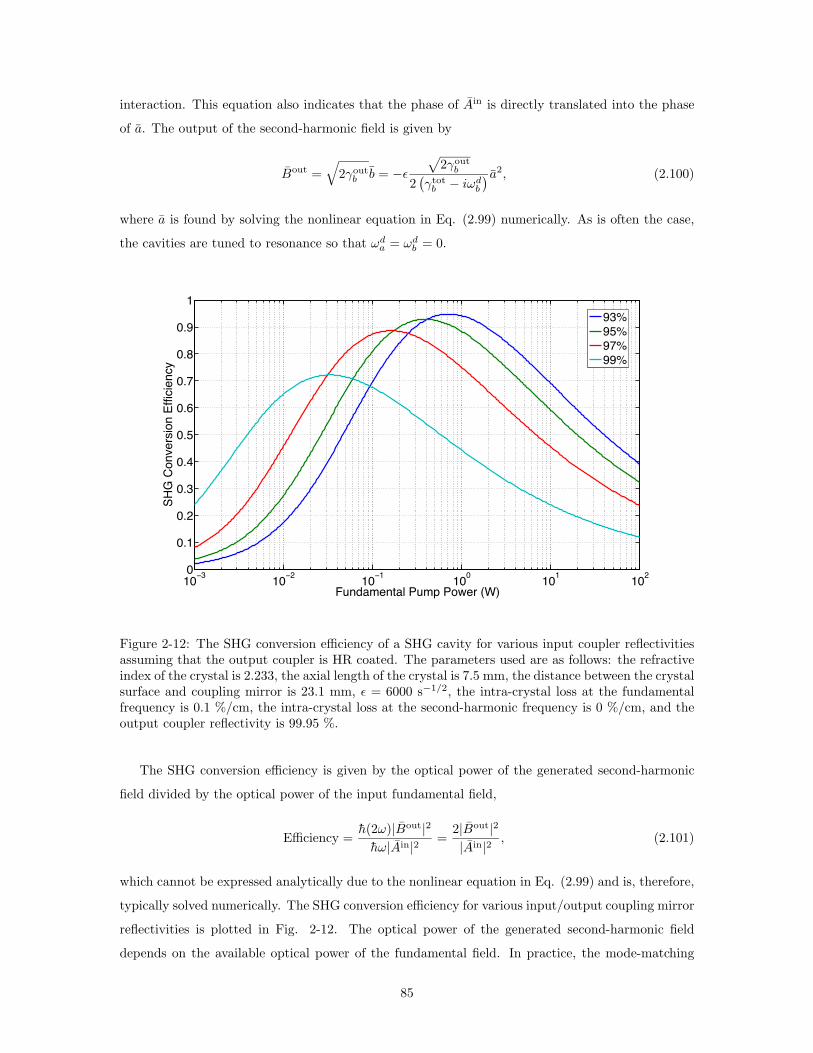
interaction. This equation also indicates that the phase of Ain is directly translated into the phase

of a. The output of the second-harmonic field is given by

Bout =√

2γoutb b = −ε

√

2γoutb

2(

γtotb − iωd

b

) a2, (2.100)

where a is found by solving the nonlinear equation in Eq. (2.99) numerically. As is often the case,

the cavities are tuned to resonance so that ωda = ωd

b = 0.

10−3 10−2 10−1 100 101 1020

0.1

0.2

0.3

0.4

0.5

0.6

0.7

0.8

0.9

1

Fundamental Pump Power (W)

SHG

Con

vers

ion

Effic

ienc

y

93%95%97%99%

Figure 2-12: The SHG conversion efficiency of a SHG cavity for various input coupler reflectivitiesassuming that the output coupler is HR coated. The parameters used are as follows: the refractiveindex of the crystal is 2.233, the axial length of the crystal is 7.5 mm, the distance between the crystalsurface and coupling mirror is 23.1 mm, ε = 6000 s−1/2, the intra-crystal loss at the fundamentalfrequency is 0.1 %/cm, the intra-crystal loss at the second-harmonic frequency is 0 %/cm, and theoutput coupler reflectivity is 99.95 %.

The SHG conversion efficiency is given by the optical power of the generated second-harmonic

field divided by the optical power of the input fundamental field,

Efficiency =h(2ω)|Bout|2

hω|Ain|2=

2|Bout|2

|Ain|2, (2.101)

which cannot be expressed analytically due to the nonlinear equation in Eq. (2.99) and is, therefore,

typically solved numerically. The SHG conversion efficiency for various input/output coupling mirror

reflectivities is plotted in Fig. 2-12. The optical power of the generated second-harmonic field

depends on the available optical power of the fundamental field. In practice, the mode-matching

85

efficiency of the mode of the fundamental field to the cavity mode needs to be taken into consideration

to estimate the right optical power coupled to the SHG cavity.

2.4.7 Classical Optical Parametric Oscillation

Before generating squeezed states, it is convenient to examine the classical behavior of an OPO to

optimize the coupling of the pump field to the vacuum seed. This is usually done by optimizing

the parametric amplification of a bright seed when pumping the OPO. In a DOPO cavity, the

coherent intra-cavity field at the fundamental frequency is obtained from Eq. (2.97) and its complex

conjugate,

0

0

=

−γtota εb

εb∗ −γtota

a

a∗

+√

2γina

Ain

Ain

, (2.102)

where we have assumed that there is no cavity detuning and the classical amplitude Ain is real

without the loss of generality. Solving the equations for a and using the transmitted field Aout =√

2γouta a yield

Aout = 2√

ηinηout1 + xeiφ

1 − x2Ain, (2.103)

where ηin ≡ γina /γtot

a . The parametric gain is defined by

G =|Aout(x)|2

|Aout(0)|2=

1 + x2 + 2x cosφ

(1 − x2)2, (2.104)

which can be greater or smaller than 1, depending on the phase φ. If φ = 0, then G = 1/(1 − x)2,

which indicates parametric amplification. If φ = π, then G = 1/(1+x)2, which indicates parametric

deamplication. The parametric gain as a function of the pump power is plotted in Fig. 2-13.

2.4.8 Designing Stable Resonators with Nonlinear Media

Cavities with High Refractive Index Media

The resonator stability condition for an empty cavity with two mirrors as described in Refs. [152, 153]

cannot be applied to a cavity with a crystal due to its high refractive index that slows down the

propagation of light in the material. In this section, a more generalized resonator stability condition

for such cavities is derived. It will be shown that in the limit of n = 1, the condition reduces to the

condition for empty cavities as expected.

A cavity composed of two curved mirrors and a crystal in between them is schematically shown

in Fig. 2-14. For a stable resonator, the wavefront R(z) of a Gaussian beam must match the mirror

86

0 0.1 0.2 0.3 0.4 0.5 0.6 0.7 0.8 0.9 110−1

100

101

102

103

104

105

106

x

Para

met

ric G

ain

Parametric Amplification

Parametric Deamplification

Figure 2-13: The parametric gain obtained through an OPO cavity. If φ = 0, parametric amplifica-tion occurs. If φ = π, parametric deamplification occurs.

curvature at each mirror. Assume that the beam waist is located exactly at the middle point of the

crystal in order to maximize the nonlinear interaction in the case of a nonlinear crystal as a high

refractive index material.

n

l

d1 d2

R1 R2

Figure 2-14: An optical cavity composed of two external mirrors and a crystal in between them.The refractive index and length of the crystal are n and l. The radii of curvature of the mirrors areR1 and R2, respectively.

Starting with waist size ω0 at the center of the crystal and propagating toward the mirror R1,

the ABCD matrices for free space with index n and distance l/2, the interface from index n to index

1, and free space with index 1 and distance d1 are respectively given by [153, 154, 152]

M1 =

1 l2n

0 1

, M2 =

1 0

0 n

, M3 =

1 d1

0 1

. (2.105)

87

The combined ABCD matrix is therefore found to be

M = M3M2M1 =

1 d1

0 1

1 0

0 n

1 l2n

0 1

=

1 l2n + nd1

0 n

. (2.106)

The spot size ω1 and the radius of curvature R1 of the beam at d1 are given by

q1 =Aq0 + B

Cq0 + D, (2.107)

where

1

q0= −i

λ

nπω20

,1

q1=

1

R1− i

λ

πω21

. (2.108)

The real and imaginary parts in Eq. (2.107) yield

l

2n+ nd1 =

nπ2ω41R1

π2ω41 + λ2R2

1

,nπω2

0

λ=

nπλω21R2

1

π2ω41 + λ2R2

1

. (2.109)

The corresponding equations for the spot size ω2 and the radius of curvature R2 of the beam at d2

are similarly given by

l

2n+ nd2 =

nπ2ω42R2

π2ω42 + λ2R2

2

,nπω2

0

λ=

nπλω22R2

2

π2ω42 + λ2R2

2

. (2.110)

Using the definitions

L1 ≡ l

2n2+ d1, L2 ≡ l

2n2+ d2, (2.111)

which we call the “effective” distances that are not equal to the physical distances, the waist size ω0

is found to be

ω40 =

λ2

π2L1(R1 − L1) =

λ2

π2L2(R2 − L2). (2.112)

If we also define the “effective” total distance between the mirrors by

Leff ≡ L1 + L2 =l

n2+ d1 + d2, (2.113)

L1 and L2 can be rewritten in terms of Leff , R1, and R2 as

L1 =R2 − Leff

R1 + R2 − 2LeffLeff , L2 =

R1 − Leff

R1 + R2 − 2LeffLeff . (2.114)

It is important to note that n2 in Eq. (2.113) comes from two effects: one factor of n is due to the

88

slow propagation and the other factor of n is due to the refraction at the interface from index n to

index 1. As n → 1, the effective distance reduces to the physical distance L.

Resonator Stability Condition

Likewise, if we define the “effective” g parameters by

geff1 ≡ 1 − Leff

R1, geff

2 ≡ 1 − Leff

R2, (2.115)

the waist size ω0 and the spot sizes, ω1 and ω2, are respectively found in terms of the effective g

parameters and the effective total distance Leff (similar to the equations in Refs. [152, 153]) to be

ω20 =

Leffλ

π

√

geff1 geff

2 (1 − geff1 geff

2 )

(geff1 + geff

2 − 2geff1 geff

2 )2(2.116)

and

ω21 =

Leffλ

π

√

geff2

geff1 (1 − geff

1 geff2 )

, ω22 =

Leffλ

π

√

geff1

geff2 (1 − geff

1 geff2 )

. (2.117)

It is obvious from Eqs. (2.116) and (2.117) that real and finite solutions for the Gaussian beam

parameters and spot sizes can exist only if the effective g parameters are confined to a stability range

defined by

0 < geff1 geff

2 < 1. (2.118)

This is the resonator stability condition for cavities with high refractive index media such as nonlinear

crystals.

For nonlinear interactions through nonlinear crystals contained inside cavities such as OPO and

SHG, the waist size ω0 needs to be considered as well as the cavity stability because the strength

of the interaction is inversely proportional to the waist size ω0. In general, it is difficult to satisfy

both requirements. If the waist size is made small to maximize the nonlinear interaction, the cavity

becomes near-concentric, and therefore, unstable since geff1 geff

2 is very close to 1. If the cavity is

made stable, the waist size needs to be large, resulting in decrease in the strength of the nonlinear

interaction which is proportional to the intensity.

The generalized resonator stability condition and waist size allow us to visualize the requirements.

They are useful since the design of an OPO or SHG cavity is a delicate issue. Fig. 2-15 shows an

example of a symmetric cavity with a nonlinear crystal in between two cavity mirrors.

89

1 2 3 4 5 6 7 8 9 10−0.5

0

0.5

1

1.5

2

g 1eff g 2ef

f

1 2 3 4 5 6 7 8 9 100

20

40

60

d1 (mm)

ω0 (µ

m)

Figure 2-15: geff1 geff

2 and the waist size ω0 as functions of the distance between the crystal face andthe end mirror d1 in the case of a symmetric cavity (d1 = d2). The radii of curvature of the mirrorsare R1 = R2 = 10 mm. The refractive index of the material is 1.8. To satisfy both requirementsthat the 0 < geff

1 geff2 < 1 and the waist size is small, it is optimal to choose 4 - 8 mm for d1, taking

into account that d1 < 3 mm is too close to the crystal face to be practical.

2.5 Degradation of Squeezed States

A squeezed state is a manifestation of the sum of correlated quantum sidebands centered around the

frequency of a carrier field, as described in Sec. 2.3. The quantum correlation, however, degrades or

decoherence occurs when it interacts with the universe through losses, assuming that the universe

consists of random vacuum fields. The beamsplitter model of optical losses or decoherence is often

used to understand the interaction of squeezed states with the universe [134, 137, 142]. In this

section, the beamsplitter model is reviewed to see how the level of squeezing decreases.

Ain Aout

δv

Loss

Beamsplitter

ηloss

Figure 2-16: A beamsplitter model of squeezing degradation. Ain, Aout, and δv are the input field,output field, and vacuum field that couples in at the unused port of the beamsplitter when an opticalloss occurs. ηloss is the power transmissivity through the beamsplitter.

90

As shown in Fig. 2-16, consider that field Ain enters a beamsplitter with power transmissivity

ηloss and the output is Aout. Any loss mechanism can be interpreted as a beamsplitter and therefore

treated in this beamsplitter model. When an optical loss occurs, a random vacuum field couples

into the incoming field at the unused port of the beamsplitter and replaces the portion of the field

that is lost by the beamsplitter. When the vacuum field is δv, the output field Aout is given by

Aout(t) =√

ηlossAin(t) + i√

1 − ηlossδv(t). (2.119)

In the frequency domain, Eq. (2.119) becomes

Aout(Ω) =√

ηlossAin(Ω) + i√

1 − ηlossδv(Ω). (2.120)

Linearizing the operators [136] and taking the fluctuation components, we find

δAout(Ω) =√

ηlossδAin(Ω) + i√

1 − ηlossδv(Ω), (2.121)

and therefore, the amplitude and phase quadrature variances of the output field, respectively, are

found to be

V out1 = ηlossV

in1 + 1 − ηloss, (2.122)

V out2 = ηlossV

in2 + 1 − ηloss. (2.123)

When the transmission is 100% or ηloss = 1, the output squeezing level is retained. When the

transmission is 0% or ηloss = 0, squeezing completely disappears as expected.

2.6 Detection of Squeezed States

2.6.1 Overview

In the previous sections, the generation and degradation of squeezed states have been discussed. In

the following sections, the detection of squeezed states with one or two photodiodes and the conver-

sion of the induced photocurrent(s) into frequency spectra are described. In squeezing experiments,

spectrum analyzers are often used to obtain quadrature variances. The detailed operation of spec-

trum analyzers to obtain quadrature variances is well-described in Ref. [137]. Two methods of detect-

ing squeezed states are introduced: (1) balanced homodyne detection [140, 141, 17, 155, 16, 156, 139]

and (2) unbalanced homodyne detection [15, 13, 14]. The balanced homodyne detection is useful

in situations where both the amplitude and phase quadrature variances of an optical field in a

squeezed state need to be studied. The unbalanced homodyne detection is the scheme used to ob-

91

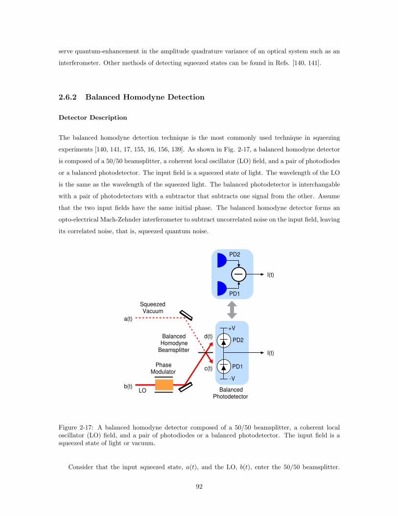
serve quantum-enhancement in the amplitude quadrature variance of an optical system such as an

interferometer. Other methods of detecting squeezed states can be found in Refs. [140, 141].

2.6.2 Balanced Homodyne Detection

Detector Description

The balanced homodyne detection technique is the most commonly used technique in squeezing

experiments [140, 141, 17, 155, 16, 156, 139]. As shown in Fig. 2-17, a balanced homodyne detector

is composed of a 50/50 beamsplitter, a coherent local oscillator (LO) field, and a pair of photodiodes

or a balanced photodetector. The input field is a squeezed state of light. The wavelength of the LO

is the same as the wavelength of the squeezed light. The balanced photodetector is interchangable

with a pair of photodetectors with a subtractor that subtracts one signal from the other. Assume

that the two input fields have the same initial phase. The balanced homodyne detector forms an

opto-electrical Mach-Zehnder interferometer to subtract uncorrelated noise on the input field, leaving

its correlated noise, that is, squeezed quantum noise.

BalancedHomodyne

Beamsplitter

+V

PD2

PD1

-V

PhaseModulator

SqueezedVacuum

LO

a(t)

b(t)

c(t)

d(t)

I(t)

PD1

PD2

I(t)

BalancedPhotodetector

Figure 2-17: A balanced homodyne detector composed of a 50/50 beamsplitter, a coherent localoscillator (LO) field, and a pair of photodiodes or a balanced photodetector. The input field is asqueezed state of light or vacuum.

Consider that the input squeezed state, a(t), and the LO, b(t), enter the 50/50 beamsplitter.

92

The output fields, c(t) and d(t), are given by

c(t)

d(t)

=1√2

1 i

i 1

a(t)

b(t)

. (2.124)

The photocurrents induced by the two photodiodes, PD1 and PD2, are given by

Ic(t) =1

2E2c†c =

E2

4(a† − ib†)(a + ib), (2.125)

Id(t) =1

2E2d†d =

E2

4(−ia† + b†)(ia + b), (2.126)

where E is given by Eq. (2.4). As in Sec. 2.3.3, we linearize the operators, a(t) and b(t), such that

a(t) → a + δa(t) and b(t) → b + δb(t). In addition, we further assume that b(t) has variable phase

θ(t) relative to a(t), such that b = (b + δb)eiθ. Then, ignoring second-order fluctuation terms such

as δa†δb, δaδb†, δb†δa, and δbδa†, Eqs. (2.125) and (2.126) become

Ic(t) =E2

4[a2 + b2 − 2ab sin θ + aδa1(t) + bδb1(t)

−a (δb1(t) sin θ + δb2(t) cos θ) − b (δa1(t) sin θ − δa2(t) cos θ)], (2.127)

Id(t) =E2

4[a2 + b2 + 2ab sin θ + aδa1(t) + bδb1(t)

+a (δb1(t) sin θ + δb2(t) cos θ) + b (δa1(t) sin θ − δa2(t) cos θ)], (2.128)

where δa1 = δa + δa†, δa2 = −i(δa − δa†), δb1 = δb + δb†, and δb2 = −i(δb − δb†) in the limiting

case of Ω + ω, as defined in Eqs. (2.50) and (2.51). Therefore, the difference photovoltage obtained

from the difference photocurrent multiplied by current-to-voltage conversion coefficient R is given

by

Vc−d = R(Ic − Id)

= −RE2

2

[

2ab sin θ + a (δb1 sin θ + δb2 cos θ) + b (δa1 sin θ − δa2 cos θ)]

, (2.129)

which can be decomposed into the time-independent DC component (first term) and the time-

dependent fluctuation component (terms containing δa1, δa2, δb1, and δb2). In the frequency domain,

the fluctuation component is given by

Vc−d(Ω) = −RE2

2

[

a(

δb1 sin θ + δb2 cos θ)

+ b (δa1 sin θ − δa2 cos θ)]

, (2.130)

93

and therefore, the variance of the photovoltage is found to be

Nc−d(Ω) =

⟨

∣

∣

∣Vc−d(Ω)

∣

∣

∣

2⟩

=R2E4

4

[

a2(

Vb1 sin2 θ + Vb2 cos2 θ)

+ b2(

Va1 sin2 θ + Va2 cos2 θ)]

. (2.131)

In most cases, the amplitude of the squeezed field is much smaller than the amplitude of the LO

(a + b). In the case of a squeezed vacuum field, it does not contain any coherent amplitude (a = 0).

Thus, Eq. (2.131) becomes

Nc−d(Ω) % R2E4b2

4

(

Va1(Ω) sin2 θ + Va2(Ω) cos2 θ)

. (2.132)

Since Va1(Ω) = Va2(Ω) = 1 at all frequencies when the input field is blocked so that a random

vacuum field enters the balanced homodyne detector, the normalized variance of the input squeezed

field can be obtained by dividing the variance of the photovoltage when the input field is unblocked

by the variance when it is blocked, such that

V θa (Ω) ≡

Nc−d(Ω)∣

∣

∣

Unblocked

Nc−d(Ω)∣

∣

∣

Blocked

= Va1(Ω) sin2 θ + Va2(Ω) cos2 θ. (2.133)

As shown in the derivation, the biggest advantages of the balanced homodyne detector are the

cancellation of classical noise on the LO and the measurement of the linear response of the input

squeezed field so that both amplitude and phase quadratures can be observed. If the beamsplitter is

not perfectly balanced, the subtraction of the classical noise becomes imperfect, leaving some excess

noise in the squeezing spectrum, especially at low frequencies.

Detection Efficiency

So far we have assumed that the mode overlap between the input squeezed light and LO is perfect,

but this is not often the case experimentally. The homodyne efficiency is the degree of the mode

overlap between the two fields given by

ηhom =

(

Pmax − Pmin

Pmax + Pmin

)2

, (2.134)

where Pmax and Pmin are the maximum and minimum values of the interference fringe measured

by the photodetectors (assuming that both photodetectors measure the same homodyne visibility)

[137, 141].

In general, photodiodes do not convert all incident photons to electrons in the conduction band.

The quantum efficiency of photodiodes is the efficiency of the energy conversion from photons to

94

electrons, defined by8

ηPD =hc

λe

I

P, (2.135)

where c is the speed of light in vacuum, h is Planck’s constant, e is the electron charge, λ is the laser

wavelength, I is the induced photocurrent, and P is the incident optical power.

Taking into account these two effects and a possible optical loss in the path between the OPO and

homodyne detector (characterized by ηloss and following Sec. 2.5, the quadrature variance detected

by the imperfect homodyne detector is given by making the substitution V θa → ηlossηhomηPDV θ

a +1−

ηlossηhomηPD, such that when the OPO-generated squeezed field characterized by Eqs. (2.69) and

(2.70) is detected by the imperfect homodyne detector, the detected quadrature variance is given

from Eq. (2.133) by

V θa (Ω) = ηlossηhomηPD

[

Va1(Ω) sin2 θ + Va2(Ω) cos2 θ]

+ 1 − ηlossηhomηPD

= V deta1

sin2 θ + V deta2

cos2 θ, (2.136)

where the squeezed and anti-squeezed quadrature variances measured by the detector (assuming

that the amplitude quadrature is initially squeezed) are, respectively, given by

V deta1

≡ 1 − 4ηlossηoutηhomηPDx

(1 + x)2, V det

a2≡ 1 + 4ηlossηoutηhomηPD

x

(1 − x)2. (2.137)

Note that the squeezing level is completely determined by the detection efficiencies (ηhom and ηPD),

the escape efficiency ηout, the optical loss 1 − ηloss, and the nonlinear coupling efficiency x. More

details about the detection efficiencies can be found in Ref. [137].

2.6.3 Unbalanced Homodyne Detection

Detector Description

Although squeezed states can be measured by a balanced homodyne detector, it is useful only for

stand-alone squeezed state generators. When a squeezed state of light is used to reduce quantum

noise in an optical system where its field is the quantity of interest to measure, the balanced homo-

dyne detector may not be practical. This is analogous to the situation in which a squeezed state

of light is injected into the antisymmetric port of a Michelson interferometer with an offset from a

dark fringe that leaks out some amount of the carrier light that a possible GW signal beats against.

This scheme called the DC readout scheme [7, 95, 157] is planned to be used in Advanced LIGO. In

this case, another detection method is needed for this type of detection. In this section, unbalanced

8More rigorously, quantum efficiency is a quantity defined for a photosensitive device as the percentage of photonshitting the photoreactive surface that will produce an electron-hole pair.

95

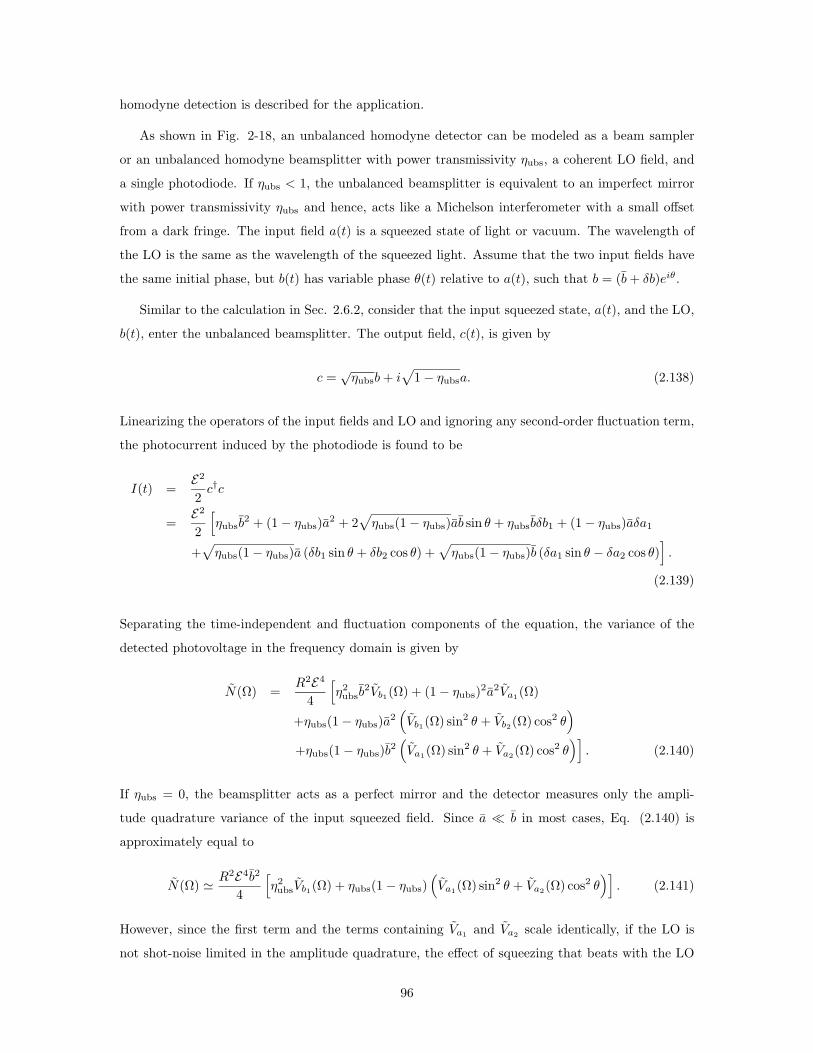
homodyne detection is described for the application.

As shown in Fig. 2-18, an unbalanced homodyne detector can be modeled as a beam sampler

or an unbalanced homodyne beamsplitter with power transmissivity ηubs, a coherent LO field, and

a single photodiode. If ηubs < 1, the unbalanced beamsplitter is equivalent to an imperfect mirror

with power transmissivity ηubs and hence, acts like a Michelson interferometer with a small offset

from a dark fringe. The input field a(t) is a squeezed state of light or vacuum. The wavelength of

the LO is the same as the wavelength of the squeezed light. Assume that the two input fields have

the same initial phase, but b(t) has variable phase θ(t) relative to a(t), such that b = (b + δb)eiθ.

Similar to the calculation in Sec. 2.6.2, consider that the input squeezed state, a(t), and the LO,

b(t), enter the unbalanced beamsplitter. The output field, c(t), is given by

c =√

ηubsb + i√

1 − ηubsa. (2.138)

Linearizing the operators of the input fields and LO and ignoring any second-order fluctuation term,

the photocurrent induced by the photodiode is found to be

I(t) =E2

2c†c

=E2

2

[

ηubsb2 + (1 − ηubs)a

2 + 2√

ηubs(1 − ηubs)ab sin θ + ηubsbδb1 + (1 − ηubs)aδa1

+√

ηubs(1 − ηubs)a (δb1 sin θ + δb2 cos θ) +√

ηubs(1 − ηubs)b (δa1 sin θ − δa2 cos θ)]

.

(2.139)

Separating the time-independent and fluctuation components of the equation, the variance of the

detected photovoltage in the frequency domain is given by

N(Ω) =R2E4

4

[

η2ubsb

2Vb1(Ω) + (1 − ηubs)2a2Va1(Ω)

+ηubs(1 − ηubs)a2(

Vb1(Ω) sin2 θ + Vb2(Ω) cos2 θ)

+ηubs(1 − ηubs)b2(

Va1(Ω) sin2 θ + Va2(Ω) cos2 θ)]

. (2.140)

If ηubs = 0, the beamsplitter acts as a perfect mirror and the detector measures only the ampli-

tude quadrature variance of the input squeezed field. Since a + b in most cases, Eq. (2.140) is

approximately equal to

N(Ω) % R2E4b2

4

[

η2ubsVb1(Ω) + ηubs(1 − ηubs)

(

Va1(Ω) sin2 θ + Va2(Ω) cos2 θ)]

. (2.141)

However, since the first term and the terms containing Va1 and Va2 scale identically, if the LO is

not shot-noise limited in the amplitude quadrature, the effect of squeezing that beats with the LO

96

is contaminated by the dominant classical noise of the LO.

+V

a(t)

b(t)c(t)

d(t)

I(t)

UnbalancedHomodyne

Beamsplitter

LO

PhaseModulator

Figure 2-18: An unbalanced homodyne detector composed of a beam sampler or an unbalancedhomodyne beamsplitter, a coherent LO field, and a single photodiode. The input field is a squeezedstate of light or vacuum.

Similar to the balanced homodyne detection, since Va1(Ω) = Va2(Ω) = 1 at all frequencies when

the input field is blocked so that a random vacuum field enters the unbalanced homodyne detector,

the normalized variance of the input squeezed field can be obtained by dividing the variance of the

photovoltage when the input field is unblocked by the variance when it is blocked, such that at

frequencies where Vb1(Ω) = 1,

V θa (Ω) ≡

N(Ω)∣

∣

∣

Unblocked

N(Ω)∣

∣

∣

Blocked

= (1 − ηubs)[

Va1(Ω) sin2 θ + Va2(Ω) cos2 θ]

+ ηubs. (2.142)

If Vb1 ) 1, assuming that the generated squeezing level is moderate, then V θa % 1, and thus, the

effect of squeezing cannot be observed.

Detection Efficiency

Similar to the balanced homodyne detection in the previous section, the detection efficiency is

determined by the mode overlap between the LO and the input squeezed field and the quantum

efficiency of the photodiode.

2.7 Control of Squeezed States

2.7.1 Overview

Squeezed states are a much utilized resource required to perform quantum non-demolition readout

[158] and to enhance the sensitivity of quantum noise limited applications [10]. The application of

97

squeezed states requires, firstly, the generation of quality squeezed states and, secondly, the readout

and control of the phase of the states, such that the appropriate quadrature is measured. When

we generate a squeezed state in a sub-threshold OPO and detect it with a homodyne detector, we

need to control the so-called squeeze angle which is defined by the difference between the semiminor

axis of the squeezed noise ball (ellipse) and the amplitude axis of a coherent field that the squeezed

field beats against. For the readout and control of squeezed states of light, information about the

squeeze angle can be obtained from the parametric amplification or deamplification of a coherent

seed field such that the standard RF modulation/demodulation or DC readout techniques can be

used to stabilize the phase [159, 137]. For quantum states which do not have a coherent amplitude

at the carrier frequency such as a squeezed state of vacuum, the standard phase-locking techniques

are not available.

In this situation, there are two available control schemes: (1) quantum noise-locking [160, 17]

and (2) coherent control of squeezing [161, 18]. In the former scheme, the squeeze angle is modulated

and the squeezing spectrum is demodulated to obtain an error signal for feedback control. In this

case, the field that carries the squeezed state can be completely devoid of a coherent amplitude. In

the latter scheme, the parametric amplification or deamplification of a coherent sideband along with

a squeezed vacuum field is measured to obtain an error signal for feedback control.

Throughout this thesis, the quantum noise-locking technique is experimentally used because it

has some advantage over the the coherent control in squeezing-enhanced laser interferometric GW

detectors. In the following sections, the two methods of controlling squeezed states of vacuum are

described.

2.7.2 Quantum Noise Locking

Introduction

An error signal for the quantum noise locking technique can be obtained for the case of locking

the squeezed vacuum phase on a homodyne detector in an analogous way to coherent modulated

techniques [162]. The squeezed vacuum phase is modulated at some frequency, and then, the noise

power detected by the homodyne detector is demodulated. This produces an error signal which has

zero crossings at both the minimum and maximum variance points. This technique, which we refer

to as quantum noise-locking or noise-locking [160], has application in the locking of the phase of

quantum states that have non-polar symmetric phase space distribution functions. This technique

has been used already in previous squeezed vacuum experiments [163, 164, 17, 155].

Moreover, in applications where the properties of squeezed vacuum states are desirable, the

noise-locking technique is a good choice for phase control. One could conceive a scheme where a

vacuum squeezed state is generated with coherent phase modulation sidebands without a coherent

98

carrier amplitude imposed on it [18]. One such application may be in laser-interferometric GW

detectors where low-frequency squeezing at the optimum phase is required. The relative immunity

of squeezed vacuum states to classical noise sources can result in squeezing being produced in the

GW detection band [17, 18, 134]. For this reason, the quantum noise-locking technique will be used

in the experiments in Chaps. 3, 4, and 6.

Noise-Locking Error Signal

In this section, the error signal of the quantum noise-locking technique is derived theoretically.

Much of the rigorous derivation is described in Ref. [160]. Fig. 2-19 shows two input fields, a and

b, with relative phase denoted θ that interfere on a balanced beamsplitter. These operators satisfy

the standard commutation relations in Eq. (1.45). The output fields, c and d, are incident on the

photodetectors (PD1 and PD2). In the case of noise-locking the phase of a squeezed vacuum field

on the homodyne detector, a is the squeezed state and b is the LO. The output of the balanced

homodyne detector is sent to a band-pass filter (BPF). The band-pass-filtered output is sent to an

envelope detector which gives an output proportional to the real envelope of the input. This signal

is then demodulated at the modulation frequency and low-pass filtered to give the error signal.

The generation of noise-locking error signals requires modulation of the relative phase between

the two input fields. The phase of the LO is modulated at frequency Ωm so that θ = θ0 +θ1 sinΩmt,

where θ0 is the average DC phase and θ1 is the modulation depth. For small modulation depth

(θ1 + θ0), we make the approximation eiθ1 sinΩmt % J0(θ1)+J1(θ1)eiΩmt−J1(θ1)e−iΩmt. If the input

squeezed field has a coherent amplitude, the DC component in Eq. (2.129) can be modulated and

the photodetector signal can be demodulated to obtain an error signal. However, in the absence of a

coherent amplitude in the squeezed vacuum field, the DC term vanishes and therefore, the correlated

noise obtained by band-pass-filtering and envelope-detecting the signal needs to be demodulated to

acquire an error signal. When the phase of the LO is modulated in the case of a = 0, the difference

photovoltage in Eq. (2.129) becomes

Vc−d = −RE2b

2[δa1(J0 sin θ0 + 2J1 cos θ0 sinΩmt) − δa2(J0 cos θ0 − 2J1 sin θ0 sinΩmt)] . (2.143)

In the frequency domain, neglecting J21 (θ0) terms, the variance of the photovoltage after band-pass-

filtering the photovoltage is given by

Nc−d(Ω) % R2E4b2

4

[

J20

(

Va1 sin2 θ0 + Va2 cos2 θ0

)

+2J0J1

(

Va1 − Va2

)

sin 2θ0 sinΩmt]

∆Ω, (2.144)

where ∆Ω is the detection bandwidth. Here we have assumed a perfect band-pass filter with hard

99

HomodyneBeamsplitter

+V

PD2

PD1

-V

BandpassFilter

EnvelopeDetector

Low-PassFilter

Mixer

Oscillator

Adder

PhaseModulator

SqueezedVacuum

LO

Monitor

a(t)

b(t)

c(t)

d(t)

PD1

PD2

BalancedPhotodetector

Figure 2-19: A balanced homodyne detector with a noise-locking servo. Two input fields, a(t) andb(t), interfere with relative phase, θ, on a balanced 50/50 beamsplitter. a(t) is a squeezed vacuumfield and b(t) is a coherent local oscillator (LO) field. Here the LO beam b(t) passes through a phasemodulator with an applied sinusoidal modulation signal at frequency Ωm/2π. The output fields,c(t) and d(t), are incident on the photodiodes, PD1 and PD2, that form a balanced photodetectorwhen PD1 and PD2 are respectively biased negatively and positively. The balanced photodetectorcan be replaced with a pair of photodetectors with a differencer that subtracts one signal from theother. To derive the noise-locking error signal, the output of the homodyne is band-pass-filtered(BPF), and then envelope-detected (ED). The output of the envelope detector is demodulated atthe modulation frequency, and then low-pass filtered (LPF), yielding a control signal that is fed backto the phase modulator.

edges although experimentally this is not the case. Demodulating Eq. (2.144) at Ωm and low-pass

filtering its output to remove sinΩmt and sin 2Ωmt terms yields the noise-locking error signal,

κ =J0(θ1)J1(θ1)R2E4b2

2

(

Va1 − Va2

)

∆Ω sin 2θ0, (2.145)

which has zero crossings at θ0 = 0 and π/2. The error signal amplitude depends on the quadrature

variances and their asymmetry. Thus, if there is no asymmetry in the quadrature variances (Va1 =

Va2 = 1), the error signal vanishes. The error signal compared with the quadrature variance of a

squeezed vacuum field is shown in Fig. 2-20.

Stability of Noise-Locking

Since it is the variance or noise power of the detected squeezed vacuum field which is used to derive

the error signal, the noise performance of the squeeze angle control depends on the variance of the

100

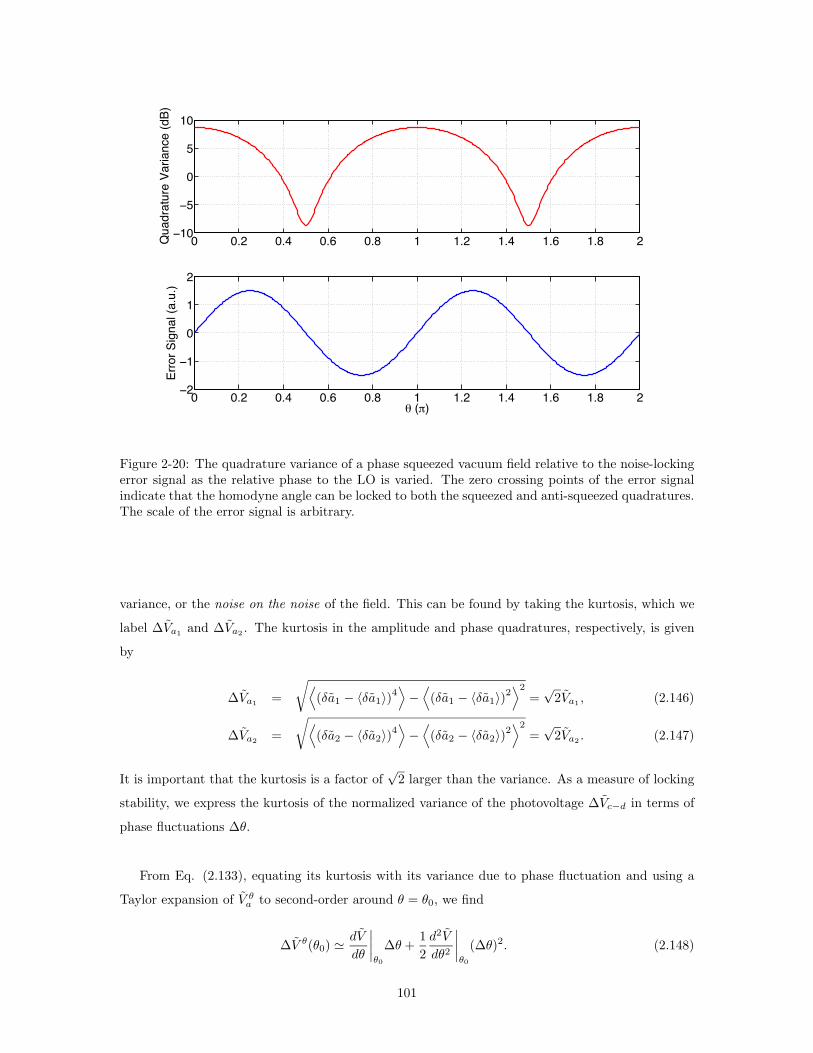
0 0.2 0.4 0.6 0.8 1 1.2 1.4 1.6 1.8 2−2

−1

0

1

2

θ (π)

Erro

r Sig

nal (

a.u.

)

0 0.2 0.4 0.6 0.8 1 1.2 1.4 1.6 1.8 2−10

−5

0

5

10

Qua

drat

ure

Varia

nce

(dB)

Figure 2-20: The quadrature variance of a phase squeezed vacuum field relative to the noise-lockingerror signal as the relative phase to the LO is varied. The zero crossing points of the error signalindicate that the homodyne angle can be locked to both the squeezed and anti-squeezed quadratures.The scale of the error signal is arbitrary.

variance, or the noise on the noise of the field. This can be found by taking the kurtosis, which we

label ∆Va1 and ∆Va2 . The kurtosis in the amplitude and phase quadratures, respectively, is given

by

∆Va1 =

√

⟨

(δa1 − 〈δa1〉)4⟩

−⟨

(δa1 − 〈δa1〉)2⟩2

=√

2Va1 , (2.146)

∆Va2 =

√

⟨

(δa2 − 〈δa2〉)4⟩

−⟨

(δa2 − 〈δa2〉)2⟩2

=√

2Va2 . (2.147)

It is important that the kurtosis is a factor of√

2 larger than the variance. As a measure of locking

stability, we express the kurtosis of the normalized variance of the photovoltage ∆Vc−d in terms of

phase fluctuations ∆θ.

From Eq. (2.133), equating its kurtosis with its variance due to phase fluctuation and using a

Taylor expansion of V θa to second-order around θ = θ0, we find

∆V θ(θ0) %dV

dθ

∣

∣

∣

∣

θ0

∆θ +1

2

d2V

dθ2

∣

∣

∣

∣

θ0

(∆θ)2. (2.148)

101

Expanding both sides, the equation becomes

√2(Va1 sin2 θ0 + Va2 cos2 θ0) =

∣

∣

∣(Va1 − Va2) sin 2θ0∆θ + (Va1 − Va2) cos 2θ0(∆θ)2

∣

∣

∣, (2.149)

which when solved for ∆θ at the two locking points (θ0 = 0,π/2) yields

∆θ|θ0=π/2 =

√ √2Va1

Va2 − Va1

, (2.150)

∆θ|θ0=0 =

√ √2Va2

Va2 − Va1

. (2.151)

In the case of perfect squeezing in the amplitude quadrature with a squeeze factor of r, taking into

account that the variance is proportional to ∆Ω and the kurtosis is proportional to√

∆Ω, Eqs.

(2.150) and (2.151) become

∆θ|θ0=π/2 ∝√

1

e4r − 1

(

2

∆Ω

)1/4

, (2.152)

∆θ|θ0=0 ∝√

1

1 − e−4r

(

2

∆Ω

)1/4

. (2.153)

If the detection efficiency ηdet is taken into account, the amplitude and phase quadrature variances

are given by Va1 = ηdete−2r + 1 − ηdet and Va2 = ηdete2r + 1 − ηdet, and then, Eqs. (2.152) and

(2.153) become

∆θ|θ0=π/2 ∝

√

ηdete−2r + 1 − ηdet

ηdet(e2r − e−2r)

(

2

∆Ω

)1/4

, (2.154)

∆θ|θ0=0 ∝

√

ηdete2r + 1 − ηdet

ηdet(e2r − e−2r)

(

2

∆Ω

)1/4

. (2.155)

The stability of the two locking points is plotted as a function of squeeze factor r in Fig. 2-21.

For both the squeezed and anti-squeezed quadratures, the stability of the noise-locking improves as

the squeeze factor is increased. This is not surprising since it is from the quadrature asymmetry

that the error signal is derived. Eqs. (2.152) and (2.153) show that the locking stability for both

quadratures improves as the detection bandwidth is increased, albeit with a weak dependence.

2.7.3 Coherent Control of Squeezing

Introduction

Although the noise-locking technique is powerful in that it does not require any coherent fields, its

stability is limited by the kurtosis of the squeezed vacuum field. The coherent control technique is

102

0 0.2 0.4 0.6 0.8 1 1.2 1.4 1.6 1.8 210

2

10 1

100

101

r

Dq (

a.u

.)

SqueezedAnti squeezed

Figure 2-21: The stability of the two locking points as a function of squeeze factor r. As r increases,the level of fluctuations in θ decreases for the squeezed quadrature and converges to unity for theanti-squeezed quadrature.

another useful method of locking the squeeze angle of a squeezed vacuum field that beats with a

coherent LO field [161]. A subcarrier field which is frequency-shifted by Ωs from the carrier frequency

is injected into an OPO cavity within its linewidth. Due to the nonlinear interaction between the

subcarrier as a signal field at frequency ω + Ωs and the pump field at frequency 2ω, the difference

frequency generation takes place in the NDOPO, yielding the idler field at frequency ω−Ωs that is

correlated with the signal. Since squeezing is a representation of the quantum correlation between

upper and lower quantum sidebands centered around the carrier frequency, the coherent correlation

between the signal and idler fields can also be used to obtain information about the squeeze angle.

Once the squeezed vacuum is generated by the NDOPO along with the coherent signal and idler

fields, when it is detected by a homodyne detector with a LO field, the beat between the LO and

signal/idler can be used to obtain the homodyne angle.

Error Signal for Squeeze Angle Control

Assuming that γins % γin

i , γouts % γout

i , and the amplitude of the input signal field is real without the

loss of generality, from Eqs. (2.37) and (2.45), the amplitudes of the output fields are given by

Aouts

Aout∗i

= 2√

γina γout

a

γtota − 1

2E b

− 12E b∗ γtot

a

−1

Ains

0

, (2.156)

103

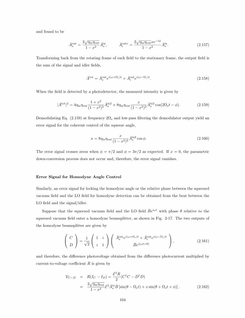
and found to be

Aouts =

2√

ηinηout

1 − x2Ain

s , Aout∗i =

2√

ηinηoutxe−iφ

1 − x2Ain

s . (2.157)

Transforming back from the rotating frame of each field to the stationary frame, the output field is

the sum of the signal and idler fields,

Atot = Aouts ei(ω+Ωs)t + Aout

i ei(ω−Ωs)t. (2.158)

When the field is detected by a photodetector, the measured intensity is given by

|Atot|2 = 4ηinηout1 + x2

(1 − x2)2Ain2

s + 8ηinηoutx

(1 − x2)2Ain2

s cos(2Ωst − φ). (2.159)

Demodulating Eq. (2.159) at frequency 2Ωs and low-pass filtering the demodulator output yield an

error signal for the coherent control of the squeeze angle,

κ = 8ηinηoutx

(1 − x2)2Ain2

s cosφ. (2.160)

The error signal crosses zeros when φ = π/2 and φ = 3π/2 as expected. If x = 0, the parametric

down-conversion process does not occur and, therefore, the error signal vanishes.

Error Signal for Homodyne Angle Control

Similarly, an error signal for locking the homodyne angle or the relative phase between the squeezed

vacuum field and the LO field for homodyne detection can be obtained from the beat between the

LO field and the signal/idler.

Suppose that the squeezed vacuum field and the LO field Beiωt with phase θ relative to the

squeezed vacuum field enter a homodyne beamsplitter, as shown in Fig. 2-17. The two outputs of

the homodyne beamsplitter are given by

C

D

=1√2

1 i

i 1

Aouts ei(ω+Ωs)t + Aout

i ei(ω−Ωs)t

Bei(ωt+θ)

, (2.161)

and therefore, the difference photovoltage obtained from the difference photocurrent multiplied by

current-to-voltage coefficient R is given by

VC−D = R(IC − ID) =E2R

2(C†C − D†D)

=2√

ηinηout

1 − x2E2Ain

s B [sin(θ − Ωst) + x sin(θ + Ωst + φ)] . (2.162)

104

Demodulating Eq. (2.162) at frequency Ωs and low-pass filtering the demodulator output yield an

error signal,

κ =2√

ηinηout

1 − x2E2Ain

s B [sin θ + x sin(θ + φ)] . (2.163)

The combination of both error signals in Eqs. (2.160) and (2.162) gives an error signal for controlling

the homodyne angle, θ.

105

Chapter 3

Experimental Generation,

Detection, and Control of

Squeezed States

3.1 Overview

In the previous chapter, the generation, degradation, detection, and control of squeezed states

using a sub-threshold optical parametric oscillator (OPO) with a second-order nonlinear medium

and a homodyne detector have been theoretically introduced. In this chapter, the experimental

demonstration of the generation, detection, and control of squeezed states is presented. We focus

on the generation of squeezed states using a periodically-poled KTiOPO4 (PPKTP) crystal in a

quasi-phase-matched OPO in a linear traveling-wave cavity configuration. The reasons for choosing

PPKTP as a nonlinear medium and the optical configuration will be explained in Chap. 4. In Sec.

3.2, the apparatus of a squeezed vacuum generator built in the Caltech 40m lab [165] is described1.

In Sec. 3.3, experimental results of squeezing are presented.

3.2 Experimental Apparatus

3.2.1 Overview

As schematically shown in Fig. 3-1, the squeezed vacuum generator – or squeezer – consists of (1)

a laser source, (2) a second-harmonic generator (SHG), (3) an optical parametric oscillator (OPO),

1Although a few different squeezers (mainly with different crystals) have been built during my Ph.D., the latestsqueezer built at Caltech is mainly discussed in this chapter. Some results presented in this chapter come from theprevious squeezers, but the overall performance of squeezing is intact.

107

PO

AuxiliaryNd:YAG LASER

PO

Fiber InputCoupler

PO

FaradayIsolator

FaradayIsolator

BS

BS

PBSDBS

DBS

PM1

PM2

FaradayIsolator

Fiber OutputCoupler

PZT1

PZT2

Fiber Mode Cleaner

PZT3

BS

PD2

PD3

HPD1

HPD2

PD1

λ/2

λ/2

OPO

SHG

PZT4

Beam Dump

Beam Dump

Nd:YAGMOPA LASER

SpectrumAnalyzer

Subtractor

S

S

S

Figure 3-1: A schematic of the squeezer. SHG: second-harmonic generator, OPO: optical paramet-ric oscillator, PM1 and PM2: phase modulators, PZT1-4: piezo-electric transducers, DBS: dichroicbeamsplitter, λ/2: half-wave plate, PBS: polarizing beamsplitter, BS: 50/50 beamsplitter, PO: pick-off beam sampler, PD1-3: photodetectors, HPD1 and HPD2: homodyne photodetectors. Spectrumanalyzers HP8591E (Hewlett-Packard) and SR785 (Stanford Research Systems) are used to measurethe response of the homodyne detector at MHz and lower frequencies respectively.

(4) subcarrier optics, (5) a homodyne detector with a mode-cleaned local oscillator (LO) field, and

(6) feedback control systems to lock the SHG and OPO cavities and the squeeze angle. Simply put,

the OPO pumped by a second-harmonic field generated by the SHG produces a squeezed vacuum

field, which is then detected by the homodyne detector with the LO. In the following sections, the

roles and properties of each major component are described.

3.2.2 Laser

The main laser source that powers the squeezer is a single-frequency Nd:YAG Master Oscillator

Power Amplifier (MOPA) laser in which a Lightwave 126 (Lightwave Inc.) master laser is amplified

by a series of laser amplifiers. The laser wavelength is 1064 nm. The output of the MOPA laser is

about 6 W, and about 1.5 W of it is utilized for the SHG, OPO, and other optics in the squeezer.

Although a pre-stabilized laser system [166] is available at the Caltech 40m lab [165], it is not

necessary for the generation of squeezed states, and thus, it is not discussed here.

108

PhaseModulator

DichroicMirror

OutputCoupler

PZTMgO:LiNbO 3

Photodetector

Oven

Mixer

Low-PassFilter

High VoltageAmplifier

Oscillator

SecondHarmonic

Field

FundamentalField

Low-PassFilter

DifferentialAmplifier

SettingTemperature

Thermistor Heater

Figure 3-2: A detailed schematic of the SHG that consists of a 5% MgO:LiNbO3 crystal and anexternal coupling mirror. The reflectivity of the mirror is 95.0% at 1064 nm and 4.0% at 532 nm.The reflectivity of the curved surface of the crystal is 99.95% at both 1064 nm and 532 nm. Thus,the SHG forms a cavity at 1064 nm, but not at 532 nm. The SHG cavity is locked on resonance bythe transmission PDH locking technique. The temperature of the crystal is also controlled by thefeedback control system using a PID controller.

3.2.3 Second-Harmonic Generator

The role of the SHG is to generate a second-harmonic field to pump the OPO. A detailed schematic

of the SHG is shown in Fig. 3-2. The SHG is a cavity composed of a 5% MgO:LiNbO3 hemilithic

crystal (Photon LaserOptik Inc.) and an external coupling mirror. One surface of the crystal is flat

and AR coated. The other surface is curved with a radius-of-curvature of 8 mm and its reflectivity is

99.95% at both 1064 nm and 532 nm. The coupling mirror has a radius-of-curvature of 50 mm and

is located at 48 mm from the center of the crystal. Its reflectivities are 95.0% at 1064 nm and 4.0%

at 532 nm. It is mounted on a piezo-electric transducer (PZT) as an actuator that adjusts the cavity

length to resonance at 1064 nm. The SHG cavity is locked by the transmission Pound-Drever-Hall

(PDH) technique in which the 1064 nm transmission through the SHG cavity is demodulated at the

frequency at which the phase of the 1064 nm pump is modulated and the mixer output is low-pass

filtered and fed back to the PZT after some amplification. The crystal is enclosed in an oven heated

by a current-driven NiCr wire and is maintained at 114.05 C to optimize the SHG conversion

efficiency for type I phase-matching in which the fundamental field is polarized in the ordinary axis

of the crystal while the second-harmonic field is polarized in the extraordinary axis. When the

temperature is optimized, their matched refractive index is 2.23. The measured dependence of the

109

SHG conversion efficiency on the temperature of the crystal is shown in Fig. 3-3. As compared to

the single-pass SHG conversion efficiency in Fig. 2-7, the measured SHG conversion efficiency does

not show a clear sinc function that has been predicted in Sec. 2.4.4. This is due to the dependence

of the cavity-SHG conversion efficiency on the fundamental pump power as shown in Fig. 2-12.

104 106 108 110 112 114 116 1180

1

2

3

4

5

6

7

8

9

Temperature (°C)

Seco

nd H

arm

onic

Powe

r (a.

u.)

Figure 3-3: The measured dependence of the SHG conversion efficiency on the temperature of thecrystal. As compared to the single-pass SHG conversion efficiency in Fig. 2-7, the measured SHGconversion efficiency does not show a clear sinc function that has been predicted in Sec. 2.4.4. Thisis due to the dependence of the cavity-SHG conversion efficiency on the fundamental pump poweras shown in Fig. 2-12.

The SHG cavity is pumped by 1.2 W of the MOPA laser at 1064 nm and generates 350 mW at 532

nm, which is then used to pump the OPO cavity. The cavity size of 20 mm - 60 mm is often chosen

because both the fundamental and second-harmonic fields diverge significantly at large distances due

to their small waist sizes. The mode structure of the SHG cavity using the fundamental field and

the corresponding modes of the second-harmonic field are shown in Fig. 3-4. The mode structure

of the generated second-harmonic field is also shown.

3.2.4 Optical Parametric Oscillator

The role of the OPO is to produce squeezed states of vacuum, and therefore, the OPO is the

core of the experiment. A detailed schematic of the OPO is shown in Fig. 3-5. The OPO is a

cavity composed of a 10 mm long, quasi-phase-matched, domain-engineered PPKTP crystal (Raicol

Inc.) with AR coated flat surfaces and two external coupling mirrors with radii-of-curvature of 10

110

−6 −4 −2 0 2 4 6−5

0

5

10

15

Pum

p Tr

ansm

issio

n (a

.u.)

−6 −4 −2 0 2 4 6−0.2

0

0.2

0.4

0.6

Cavity Length (a.u.)Seco

nd H

arm

onic

Powe

r (a.

u.)

Figure 3-4: The mode structure of the SHG cavity using the fundamental transmission and thecorresponding modes of the second-harmonic field. The evident modes are TEM00 modes. Highermodes of the cavity are suppressed by optimizing the transmission of the TEM00 modes. The reasonwhy a few higher modes are present in the pump transmission, but no corresponding higher modesare present in the second-harmonic power is because the SHG cavity mirror reflectivities are chosento optimize the SHG conversion efficiency of the fundamental pump field in the optimized TEM00

transmission.

mm. The reflectivities of the input and output coupling mirrors are 99.95% at both 1064 nm and

532 nm and 92.0% at 1064 nm and 4.0% at 532 nm respectively. The OPO cavity length is 2.3

mm. The crystal is mounted on a heater that consists of a current-driven NiCr wire in an oven

and maintained at 33.5 C to optimize the 1064/532 parametric down-conversion. To optimize

the temperature, the parametric gain of a bright seed field is usually examined and maximized by

tuning the temperature. The measured dependence of the nonlinear interaction strength in the OPO

cavity on the temperature of the crystal is shown in Fig. 3-6. The OPO cavity is locked by the

transmission PDH locking technique with a frequency-shifted subcarrier which will be described in

the next section. One of the coupling mirrors is mounted on a PZT as an actuator used to keep

the cavity on resonance at 1064 nm. The pump is aligned and mode-matched to the OPO cavity

by optimizing the parametric gain. The measured dependence of the OPO parametirc gain on the

pump power is shown in Fig. 3-7.

When pumped by the second-harmonic pump at frequency 2ω, the OPO correlates upper and

lower quantum sidebands centered around the carrier frequency ω. The sum of the correlated

quantum sidebands appears as a squeezed vacuum field, as discussed in Chap. 2. In the case of

111

PhaseModulator

DichroicMirror

OutputCoupler

PZTPPKTP

Photodetector

Oven

MixerLow-PassFilter

High VoltageAmplifier

Oscillator

SecondHarmonic

Field

SubcarrierField

Low-PassFilter


SettingTemperature

Thermistor

Heater

Polarizer

InputCoupler

SqueezedVacuum

Figure 3-5: A detailed schematic of the OPO that consists of a periodically-poled KTiOPO4 (PP-KTP) crystal and two coupling mirrors. Both surfaces of the crystal are AR coated. The reflectivitiesof the input and output coupler are 99.95% at both 1064 nm and 532 nm and 92.0% at 1064 nmand 4.0% at 532 nm respectively, and therefore, the OPO forms a cavity at 1064 nm, but not at532 nm. The subcarrier field is used to lock the OPO cavity using the transmission PDH lockingtechnique. The polarization of the subcarrier is orthogonal to that of the squeezed vacuum field.The subcarrier is frequency-shifted relative to the fundamental field so that the vacuum field atthe fundamental frequency can resonate and interact with the second-harmonic pump in the OPOcavity. The temperature of the PPKTP crystal is maintained stable by the feedback control systemusing a PID controller.

generating squeezed vacuum as opposed to squeezed light, the seed field that couples into the cavity

from the input coupler contains no coherent amplitude, and therefore the squeeze angle which is

defined by the angle between the amplitude axis and the squeeze axis or the semiminor axis of the

noise ellipse does not exist unless the squeezed vacuum beats with a coherent field.

3.2.5 Subcarrier Optics

The role of the subcarrier is to lock the OPO cavity on resonance for the stable generation of squeezed

states. A coherent seed at the carrier frequency cannot be used as a locking probe field because

it contaminates squeezing at low frequencies due to its laser excess noise. Instead, a frequency-

shifted subcarrier field which is orthogonally polarized to the squeezed vacuum can be used as a

locking probe. There are two possible ways to generate such a subcarrier field: (1) an acousto-optic

modulator (AOM), and (2) a second laser. The first scheme is useful if the closest usable mode is near

112

20 25 30 35 40 450

5

10

15

20

25

30

35

40

Temperature (°C)

Seco

nd H

arm

onic

Powe

r (a.

u.)

Figure 3-6: The measured dependence of the nonlinear interaction strength in the OPO cavity on thetemperature of the crystal. This is obtained by using the OPO cavity as a SHG and measuring thegenerated second-harmonic power. As discussed in the previous section, the measured temperaturedependence does not show a clear sinc function due to the dependence of the cavity-SHG (notsingle-pass SHG) conversion efficiency on the fundamental pump power. The nonlinear interactiontemperature range of PPKTP is much larger than that of MgO:LiNbO3.

the carrier frequency. In general, since the OPO cavity length is short, the free spectral range (FSR)

is about 5 - 10 GHz, and therefore, the usable modes tend to be away from the carrier frequency by

several GHz or so. If an AOM for such a high frequency-shift is available, the first scheme can be

used. Double-passing a beam through an AOM is often used to obtain a high frequency-shift, but

its low diffraction efficiency at GHz frequencies might lead to a large optical loss in the frequency-

shifted subcarrier. On the other hand, the second scheme does not have this problem although the

frequency ranges of the two lasers have to overlap. However, this scheme requires the second laser

to be phase-locked to the main laser to maintain the constant frequency-shift. In this experiment,

the closest TEM00 mode in the orthogonal polarization to the squeezed vacuum is 642 MHz away

from the carrier frequency. Since such a high frequency-shift AOM is costly, the second scheme is

employed.

The second laser is also a Lightwave 126 (Lightwave Inc.) laser with a throughput of 650 mW.

About 150 mW of it is injected into the OPO cavity in the P polarization. A random vacuum

field centered around the carrier frequency enters the OPO cavity in the S polarization so that the

generated squeezed vacuum comes out of the cavity in the S polarization. A vacuum field in the

P polarization does not participate in the nonlinear optical process in the OPO cavity due to its

113

0 50 100 150 200 250 300 350 40010

1

100

101

102

103

104

105

106

Second Harmonic Pump Power (mW)

Pa

ram

etr

ic G

ain

Parametirc AmplificationParametric DeamplificationNo Pump

Figure 3-7: The measured dependence of the OPO parametric gain on the pump power. When thepump and seed are in phase in the crystal, the seed is parametrically amplified. When they are outof phase in the crystal, the seed is parametrically deamplified.

non-interacting polarization with the pump field. The OPO cavity is locked using the transmission

PDH technique in which the subcarrier is phase-modulated by an electro-optic modulator (EOM) as

a phase modulator (PM), the transmission is demodulated at the modulation frequency, yielding an

error signal, and then, the control signal is fed back to the PZT-actuated mirror of the OPO cavity.

To maintain the 642 MHz frequency-shift between the two lasers, the second laser is phase-locked

to the MOPA laser. The beat of the two lasers is detected by a PD1611 photodetector (New Focus

Inc.) with a bandwidth of 1 GHz. To maximize the beat signal with respect to the DC power of the

two lasers, their optical powers are set to be equal. The beat signal is demodulated at the frequency

of 642 MHz given by an external oscillator, yielding an error signal, and then, the produced control

signal is fed back to the piezo and thermal actuators of the second laser.

3.2.6 Homodyne Detector

The role of the homodyne detector is to measure the quadrature variance of an input squeezed field.

The homodyne detector is composed of a 50/50 beamsplitter, a pair of photodetectors (HPD1 and

HPD2), and a LO field. The difference between the two optical responses measured by the HPD1 and

HPD2 with a LO field is analyzed by spectrum analyzers HP8591E (Hewlett-Packard) and SR785

(Stanford Research Systems) at MHz and lower frequencies respectively. The homodyne beamsplitter

used in this experiment is a polarization-sensitive 50/50 beamsplitter so that the splitting ratio of

114

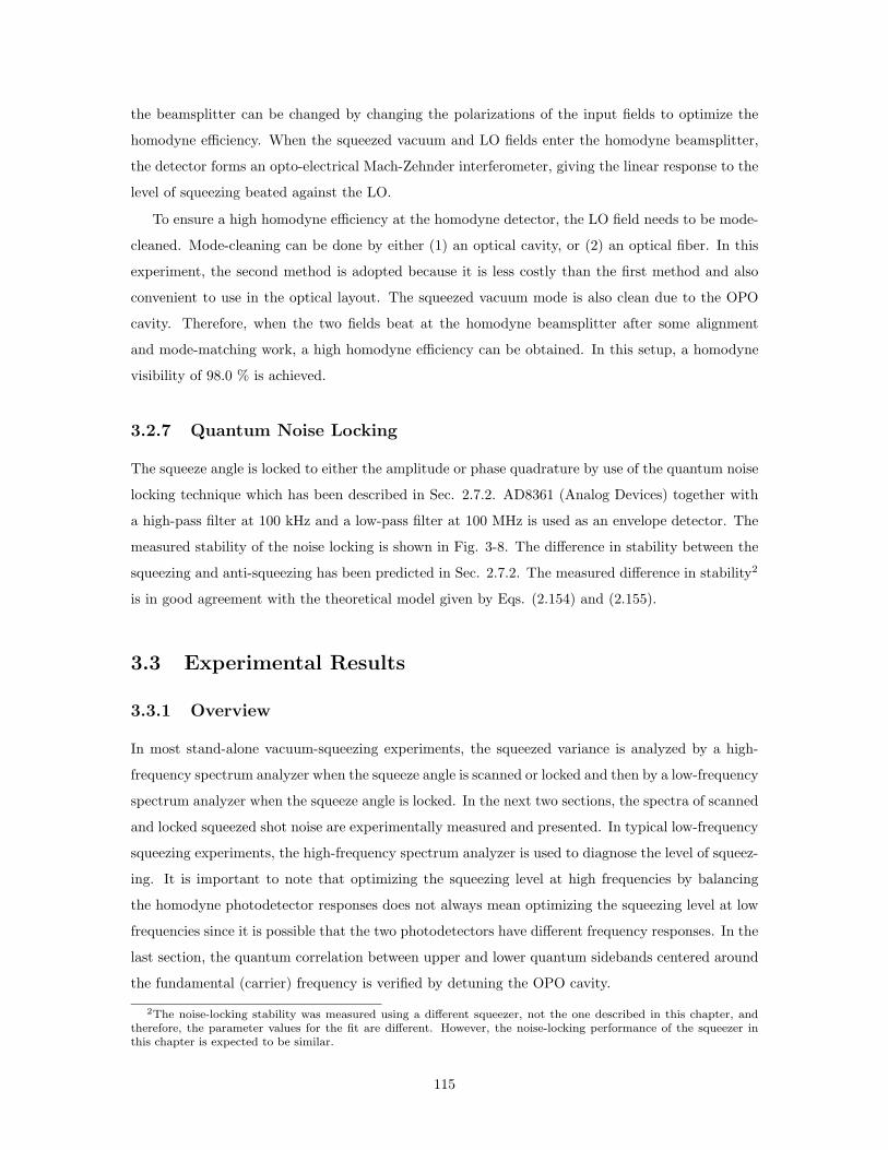
the beamsplitter can be changed by changing the polarizations of the input fields to optimize the

homodyne efficiency. When the squeezed vacuum and LO fields enter the homodyne beamsplitter,

the detector forms an opto-electrical Mach-Zehnder interferometer, giving the linear response to the

level of squeezing beated against the LO.

To ensure a high homodyne efficiency at the homodyne detector, the LO field needs to be mode-

cleaned. Mode-cleaning can be done by either (1) an optical cavity, or (2) an optical fiber. In this

experiment, the second method is adopted because it is less costly than the first method and also

convenient to use in the optical layout. The squeezed vacuum mode is also clean due to the OPO

cavity. Therefore, when the two fields beat at the homodyne beamsplitter after some alignment

and mode-matching work, a high homodyne efficiency can be obtained. In this setup, a homodyne

visibility of 98.0 % is achieved.

3.2.7 Quantum Noise Locking

The squeeze angle is locked to either the amplitude or phase quadrature by use of the quantum noise

locking technique which has been described in Sec. 2.7.2. AD8361 (Analog Devices) together with

a high-pass filter at 100 kHz and a low-pass filter at 100 MHz is used as an envelope detector. The

measured stability of the noise locking is shown in Fig. 3-8. The difference in stability between the

squeezing and anti-squeezing has been predicted in Sec. 2.7.2. The measured difference in stability2

is in good agreement with the theoretical model given by Eqs. (2.154) and (2.155).

3.3 Experimental Results

3.3.1 Overview

In most stand-alone vacuum-squeezing experiments, the squeezed variance is analyzed by a high-

frequency spectrum analyzer when the squeeze angle is scanned or locked and then by a low-frequency

spectrum analyzer when the squeeze angle is locked. In the next two sections, the spectra of scanned

and locked squeezed shot noise are experimentally measured and presented. In typical low-frequency

squeezing experiments, the high-frequency spectrum analyzer is used to diagnose the level of squeez-

ing. It is important to note that optimizing the squeezing level at high frequencies by balancing

the homodyne photodetector responses does not always mean optimizing the squeezing level at low

frequencies since it is possible that the two photodetectors have different frequency responses. In the

last section, the quantum correlation between upper and lower quantum sidebands centered around

the fundamental (carrier) frequency is verified by detuning the OPO cavity.

2The noise-locking stability was measured using a different squeezer, not the one described in this chapter, andtherefore, the parameter values for the fit are different. However, the noise-locking performance of the squeezer inthis chapter is expected to be similar.

115

102

103

10465

60

55

50

45

40

35

30

25

20

Frequency (Hz)

Err

or

Sig

na

l Sp

ect

rum

(d

Bm

)

SqueezedAnti squeezed

Figure 3-8: The stability of the noise locking technique. The noise spectrum of the noise lockingerror signal in the case of locking to the squeezed quadrature is smaller than in the case of lockingto the anti-squeezed quadrature. The theoretical model given by Eqs. (2.154) and (2.155) withthe measured efficiency of η = 0.55 and the initial squeeze factor of r = 0.9 that yields a stabilityseparation of 4.2 dB is in good agreement with the measured stability difference.

3.3.2 Spectrum of Scanned Squeezed Shot Noise

When the squeezed field has no coherent amplitude, the homodyne angle is equivalent to the squeeze

angle. The squeeze angle can be scanned by scanning either the phase of the pump field relative to

the OPO cavity (PZT3) or the phase of the LO relative to the squeezed vacuum (PZT4). In this

experiment, the second scheme (PZT4) is used because in the first scheme, the PZT could be noisy

enough to excite either the SHG or OPO cavity if it is in their vicinity.

Fig. 3-9 shows the fixed-frequency, zero-span spectra of the shot noise and squeezed/anti-

squeezed shot noise when scanning the squeeze angle at 10 Hz. The periodic oscillation of the

noise power with respect to the squeeze angle is evident in the figure. All the measurements are

done at 900 kHz with zero frequency span. The resolution bandwidth (RBW) is 100 kHz and the

video bandwidth (VBW) is 3 kHz. The squeeze angle is scanned by the PZT4 at 10 Hz, but cali-

brated to θ in the figure. The electronic noise, which consists of the electronic noise of the HPD1

and HPD2, a SR560 low-noise pre-amplifier (Stanford Research Systems) used as a subtracter with

a gain of 1000, and the SR785 spectrum analyzer, was measured to be 17.4 dB below the shot noise

level. This large separation between the shot noise level and electronic noise is sufficient to observe

squeezing without subtracting the electronic noise. The measured squeezed/anti-squeezed noise

116

0 0.5 1 1.5 2−10

−5

0

5

10

15

20

θ [π radian]

Noise

Pow

er R

elat

ive to

Sho

t Noi

se [d

B]

Shot Noise

Squeezed/AntisqueezedShot Noise

Figure 3-9: The fixed-frequency spectra of shot noise and squeezed/anti-squeezed noise power whenthe squeeze angle was scanned. The measurements were done at 900 kHz with zero frequency span.The resolution bandwidth (RBW) is 100 kHz and the video bandwidth (VBW) is 3 kHz. The squeezeangle was scanned by the PZT4 with a ramp function at 10 Hz. The electronic noise was 17.4 dBbelow the shot noise level. The measured squeezed/anti-squeezed noise power is in good agreementwith the theoretical fit (solid curve) given by Eqs. (2.132), (2.69), and (2.70) based on the measuredcomposite efficiency of η = ηoutηhomηPDηloss = 0.85. The nonlinear coupling efficiency is found fromthe fit to be x = 0.75.

power is in good agreement with the theoretical fit (solid curve) given by Eqs. (2.132), (2.69), and

(2.70) based on the measured composite efficiency of η = ηoutηhomηPDηloss = 0.85. The nonlinear

coupling efficiency is found from the fit to be x = 0.75.

There are a few important things to note: (1) the imbalance in level between the squeezing

and anti-squeezing spectra, and (2) fitting to estimate the generated level of squeezing in the OPO.

Ideally, the squeezing and anti-squeezing levels are equal in the OPO, such that ∆a1∆a2 = 1.

However, since squeezing is more susceptible to optical losses than anti-squeezing as discussed in

Sec. 2.5, the product of the amplitude and phase quadrature variances becomes greater than unity,

such that ∆a1∆a2 > 1. As for the second point, one could try to fit Eq. (2.132) with Eqs. (2.69)

and (2.70) as input quadrature variances to the squeezing/anti-squeezing spectrum. However, this

is not an easy task since as losses increase, the asymmetry between the squeezing and anti-squeezing

levels increases, making it more likely to see anti-squeezing than squeezing. If equal weight is on

each data point when fitting, it is often the case to incorrectly estimate the initial level of squeezing

in the OPO. In addition, as the squeezing level increases, there are fewer data points in the squeeze

angle range of squeezing. This makes it difficult to fit the right function to the data. For these

117

103 104 105−95

−90

−85

−80

−75

−70

Frequency [Hz]

Noise

Pow

er [d

Bm]

Squeezed Shot Noise

Shot Noise

Electronic Noise

7.4 dB

Figure 3-10: The broadband spectra of shot noise, squeezed shot noise, and electronic noise. Thespectra are averaged 2000 times. The squeeze angle is noise-locked without any coherent light.The spikes at 13.5 kHz and 15.7 kHz are due to the modulation of the PZT4 for the noise-lockingtechnique. The shot noise and squeezed shot noise spectra are in good agreement with the theoreticalpredictions (solid lines) based on the measured optical power and losses. The noise increase atfrequencies below 2 kHz in both the shot noise and squeezed shot noise spectra is due to theinadequate isolation of scattered photons (mainly from the homodyne detector) and the imperfectbalancing of the homodyne photodetector responses.

reasons, if one wants to measure the exact level of squeezing, one should lock the squeeze angle and

take the average of the squeezing data points over some period of time.

3.3.3 Spectrum of Locked Squeezed Shot Noise

When the squeeze angle is locked, a broadband squeezing spectrum can be obtained. The noise

locking technique is used, in which the squeeze angle is locked by dithering the PZT4 to obtain an

error signal and correcting the phase of the LO with the same PZT. Fig. 3-10 shows the noise power

of the squeezed and anti-squeezed shot noise when locking the squeeze angle as well as the electronic

noise of the detection system. A broadband squeezing of 7.4 ± 0.1 dB at frequencies above 3 kHz

and a cutoff frequency for squeezing at 700 Hz are evident. The spikes at 13.5 kHz and 15.7 kHz are

due to the modulation of the PZT4 for the noise-locking technique. Ignoring the low frequency noise

increase, the shot noise and squeezed shot noise spectra are in good agreement with the theoretical

predictions based on the measured optical power and losses.

The noise increase at frequencies below 2 kHz in both the shot noise and squeezed shot noise

spectra is due to the inadequate isolation of scattered photons (mainly from the homodyne detector)

118

500 550 600 650 700 750 800−4

−2

0

2

4

6

8

10

Frequency (MHz)

Noise

Pow

er R

elat

ive to

Sho

t Noi

se (d

B)

SqueezedAntisqueezed

Figure 3-11: The degradation of squeezing as a function of the detuning of the subcarrier frequency-shift. As the detuning increases, the destruction of the correlation between upper and lower quantumsidebands around the fundamental frequency leads to decrease in the squeezing level. The measureddata are compared with the theoretical fits that yield the resonance frequency to be 642.9 MHz.

and the imperfect balancing of the homodyne photodetector responses. To observe squeezing at

lower frequencies requires careful shielding of the LO or ambient light induced scattered photons

from coupling to the OPO cavity. This was demonstrated very well in Refs. [17] and [18], and is

not part of the initial goals of the present experimental demonstration.

3.3.4 Verification of Quantum Correlations

By detuning the frequency-shift of the subcarrier, the OPO cavity can be detuned with respect

to the fundamental frequency. This destroys the quantum correlation between upper and lower

quantum sidebands centered around the fundamental frequency. As discussed in Sec. 2.3.3, when

the OPO cavity is detuned continuously, the quantum correlation is weakened gradually, degrading

the overall level of squeezing in a frequency-dependent manner. The measured destruction of the

quantum correlation as a function of the detuning is shown in Fig. 3-11. The figure also shows

theoretical fits to the measured data points3. The resonance frequency is found to be 642.9 MHz

from the fits. As the detuning keeps increasing, the next TEM00 mode at one FSR away from the

resonance frequency hits resonance, and squeezing can be observed again.

3The measured maximum level of squeezing seems to be lower than the locked level of squeezing in Fig. 3-10because this measurement was taken at a different time when the squeezer was not optimized. In other words, thismeasurement was necessary before optimizing the squeezer, in order to find out the subcarrier resonance frequency.

119

Chapter 4

Requirements for Quantum

Enhanced Gravitational Wave

Detectors

4.1 Overview

The basic generation, degradation, detection, and control of squeezed states have been theoreti-

cally described in Chap. 2 and experimentally demonstrated in Chap. 3. However, although these

techniques are useful for stand-alone squeezers and quantum-enhancement in table-top scale inter-

ferometers, they are not directly applicable to quantum-enhanced laser-interferometric gravitational

wave (GW) detectors. Key requirements toward the actual implementation of quantum-enhancement

in GW detectors, such as Advanced LIGO, include (1) squeezing in the GW detection band (10 Hz

- 10 kHz), (2) a high level of squeezing (ideally 10 dB or higher)1, (3) long-term stability, and (4)

frequency-dependent squeezing. In this chapter, these four requirements are studied and solutions

to them are also presented.

4.2 Squeezing in the Gravitational Wave Band

4.2.1 Overview

The first requirement is to generate squeezed states in the GW detection band. However, this is not

an easy task because the frequency of squeezing is limited by various noise sources that couple into

an optical parametric oscillator (OPO) that generates squeezed states. The limiting noise sources

1Although this is not exactly a requirement, generating a high level of squeezing is necessary since losses in theinterferometer and injection optics attenuate some amount of squeezing.

121

are (1) seed noise [134, 17, 142], (2) pump noise [134, 167, 168, 169], (3) photothermal noise [134],

and (4) scattered photon noise [18, 17]. In the following sections, these noise sources are discussed

in detail.

4.2.2 Seed Noise

The seed noise is represented by V inA1

(Ω) and V inA2

(Ω) in Eqs. (2.65) and (2.66). When the seed is

shot-noise-limited in some frequency band so that V inA1

(Ω) = V inA2

(Ω) = 1, then squeezing is achievable

in the band. If the seed is noisy so that V inA1

(Ω) > 1 or V inA2

(Ω) > 1, the quadrature of the output

field where the input seed is noisy cannot be squeezed. Typically, the seed is not shot noise limited

at frequencies below 1 MHz due to its laser classical noise (laser amplitude and phase noise). In

most cases, this is the dominant noise that limits the frequency of squeezing. For this reason, the

generation of squeezed states has been traditionally done in the MHz regime [17, 18].

To solve this issue, a few schemes have been proposed and experimentally demonstrated. Bowen

et al. used two OPOs to cancel classical noise on a pair of squeezed light fields generated by the two

OPOs with two seeds that originate from a single laser source and share the same classical noise,

and achieved broadband squeezing at frequencies down to 220 kHz [170]. Another scheme is to use

a vacuum field at the fundamental frequency as a seed to the OPO cavity since it is in the coherent

state at all frequencies [17, 16, 18]. However, this leads to two issues: (1) the OPO cavity needs to

be controlled without coherent light in the case of a singly-resonant OPO cavity which is often used

as a squeezed state generator [13, 17, 155, 138, 139, 142], and (2) the generated squeezed vacuum

does not contain a coherent amplitude that is often used as a probe to lock the squeeze angle when

mixed with a local oscillator (LO) field.

Squeezing in the audio frequency band was first observed by McKenzie et al. [17]. They seeded a

sub-threshold OPO with a vacuum field while locking the OPO cavity manually and controlled the

homodyne angle using the quantum noise-locking technique [160]. Later, Vahlbruch et al. achieved

the generation of squeezing in the full GW detection band, using a frequency-shifted bright subcarrier

field along with the squeezed vacuum field and detecting photons generated in a nondegenerate OPO

(NDOPO) to obtain the information of the squeeze angle [18]. They used another frequency-shifted

subcarrier to lock the OPO cavity to the mode which is one free-spectral-range (FSR) away from the

carrier mode such that the vacuum field at the carrier frequency can resonate in the OPO cavity in a

TEM00 mode. Recently, a doubly-resonant OPO cavity for the production of low-frequency squeezed

states has been proposed and demonstrated [115]. This scheme does not require a subcarrier field

to lock the OPO cavity since it is done by the pump field with a phase compensation plate.

122

4.2.3 Pump Noise

The pump noise is represented by V inB1

(Ω) and V inB2

(Ω), but they do not appear in Eqs. (2.65) and

(2.66) because we have assumed |a|δb + |b|δa in the case of the undepleted pump. This assumption

is valid in most cases since typically |a| +| b| and the fluctuations in the pump and seed fields are

on the same order. However, if this is not the case, the pump noise couples into Eqs. (2.65) and

(2.66). For example, if a second-harmonic generator (SHG) is noisy and adds noise to the generated

second-harmonic field, the assumption |a|δb + |b|δa is no longer valid. The details of this case can

be found in Ref. [134].

4.2.4 Photothermal Noise

The photothermal noise arises from changes in temperature of the optical medium due to absorbed

optical power [79, 171, 172]. By nature, photothermal effects are significant at low frequencies since

thermal effects are typically slow. This effect may be significant in most nonlinear crystals since many

have relatively high absorption rates. For example, a MgO:LiNbO3 crystal has a linear absorption

rate of about 4 %/cm at 532 nm [142]. High absorption rates coupled with the high circulating power

required for strong nonlinear interaction result in a large amount of optical power absorbed into the

crystal, which may cause a significant temperature change. The average temperature change due

to the power absorbed in the crystal can be compensated for by using a temperature controller and

does not pose significant problems for most experimental systems.

Instead, we focus on the effect of photothermally induced temperature fluctuations, caused by

fluctuations in the circulating power in an OPO cavity. The circulating power fluctuations could have

both classical and quantum origins, or in the case of a shot noise limited system, only the quantum

mechanical origin. The photothermal noise caused by thermal-expansive noise and thermal-refractive

noise has two degrading effects on the production of squeezed light in the OPO. The first effect is

via fluctuations in the nonlinearity. This arises as the nonlinear strength is temperature-dependent

due to the phase-matching condition. It is a significant noise source in birefringent phase-matched

crystals since they have strong temperature dependence. The second effect is via optical path length

fluctuations. The temperature fluctuations cause the optical path length to change, potentially

causing a detuning of the optical cavity. These effects appear as 1/(Ω2 + Ω2T ) in variance, where Ω

is the sideband (measurement) frequency and ΩT is the thermal relaxation cutoff frequency of the

nonlinear medium, and are, therefore, primarily significant at low frequencies. The full derivation

of the photothermal-noise-coupled quadrature variances can be found in Ref. [134].

However, the photothermal noise can completely vanish in the absence of the bright seed since

the coupling of the photothermal noise is proportional to the seed power. In addition, by use of

quasi-phase-matched crystals instead of type I phase-matched crystals, the effect of the photothermal

123

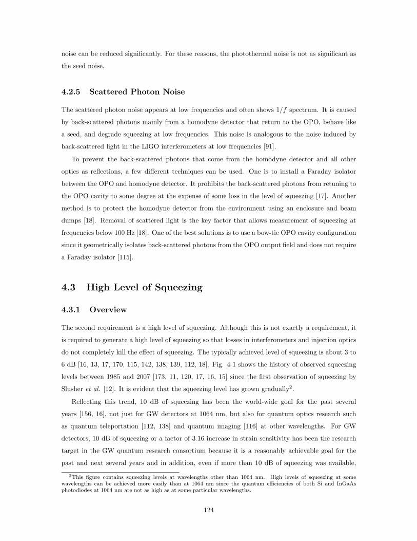
noise can be reduced significantly. For these reasons, the photothermal noise is not as significant as

the seed noise.

4.2.5 Scattered Photon Noise

The scattered photon noise appears at low frequencies and often shows 1/f spectrum. It is caused

by back-scattered photons mainly from a homodyne detector that return to the OPO, behave like

a seed, and degrade squeezing at low frequencies. This noise is analogous to the noise induced by

back-scattered light in the LIGO interferometers at low frequencies [91].

To prevent the back-scattered photons that come from the homodyne detector and all other

optics as reflections, a few different techniques can be used. One is to install a Faraday isolator

between the OPO and homodyne detector. It prohibits the back-scattered photons from retuning to

the OPO cavity to some degree at the expense of some loss in the level of squeezing [17]. Another

method is to protect the homodyne detector from the environment using an enclosure and beam

dumps [18]. Removal of scattered light is the key factor that allows measurement of squeezing at

frequencies below 100 Hz [18]. One of the best solutions is to use a bow-tie OPO cavity configuration

since it geometrically isolates back-scattered photons from the OPO output field and does not require

a Faraday isolator [115].

4.3 High Level of Squeezing

4.3.1 Overview

The second requirement is a high level of squeezing. Although this is not exactly a requirement, it

is required to generate a high level of squeezing so that losses in interferometers and injection optics

do not completely kill the effect of squeezing. The typically achieved level of squeezing is about 3 to

6 dB [16, 13, 17, 170, 115, 142, 138, 139, 112, 18]. Fig. 4-1 shows the history of observed squeezing

levels between 1985 and 2007 [173, 11, 120, 17, 16, 15] since the first observation of squeezing by

Slusher et al. [12]. It is evident that the squeezing level has grown gradually2.

Reflecting this trend, 10 dB of squeezing has been the world-wide goal for the past several

years [156, 16], not just for GW detectors at 1064 nm, but also for quantum optics research such

as quantum teleportation [112, 138] and quantum imaging [116] at other wavelengths. For GW

detectors, 10 dB of squeezing or a factor of 3.16 increase in strain sensitivity has been the research

target in the GW quantum research consortium because it is a reasonably achievable goal for the

past and next several years and in addition, even if more than 10 dB of squeezing was available,

2This figure contains squeezing levels at wavelengths other than 1064 nm. High levels of squeezing at somewavelengths can be achieved more easily than at 1064 nm since the quantum efficiencies of both Si and InGaAsphotodiodes at 1064 nm are not as high as at some particular wavelengths.

124

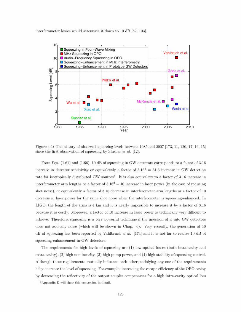
interferometer losses would attenuate it down to 10 dB [82, 103].

1980 1985 1990 1995 2000 2005 20100

2

4

6

8

10

12

Year

Sque

ezin

g Le

vel (

dB)

Slusher et al.

Vahlbruch et al.

Wu et al. McKenzie et al.

Goda et al.

Polzik et al.

Xiao et al. Goda et al.

Squeezing in Four−Wave MixingMHz Squeezing in OPOAudio−Frequency Squeezing in OPOSqueezing−Enhancement in MHz InterferometrySqueezing−Enhancement in Prototype GW Detectors

Figure 4-1: The history of observed squeezing levels between 1985 and 2007 [173, 11, 120, 17, 16, 15]since the first observation of squeezing by Slusher et al. [12].

From Eqs. (1.61) and (1.66), 10 dB of squeezing in GW detectors corresponds to a factor of 3.16

increase in detector sensitivity or equivalently a factor of 3.163 = 31.6 increase in GW detection

rate for isotropically distributed GW sources3. It is also equivalent to a factor of 3.16 increase in

interferometer arm lengths or a factor of 3.162 = 10 increase in laser power (in the case of reducing

shot noise), or equivalently a factor of 3.16 decrease in interferometer arm lengths or a factor of 10

decrease in laser power for the same shot noise when the interferometer is squeezing-enhanced. In

LIGO, the length of the arms is 4 km and it is nearly impossible to increase it by a factor of 3.16

because it is costly. Moreover, a factor of 10 increase in laser power is technically very difficult to

achieve. Therefore, squeezing is a very powerful technique if the injection of it into GW detectors

does not add any noise (which will be shown in Chap. 6). Very recently, the generation of 10

dB of squeezing has been reported by Vahlbruch et al. [174] and it is not far to realize 10 dB of

squeezing-enhancement in GW detectors.

The requirements for high levels of squeezing are (1) low optical losses (both intra-cavity and

extra-cavity), (2) high nonlinearity, (3) high pump power, and (4) high stability of squeezing control.

Although these requirements mutually influence each other, satisfying any one of the requirements

helps increase the level of squeezing. For example, increasing the escape efficiency of the OPO cavity

by decreasing the reflectivity of the output coupler compensates for a high intra-cavity optical loss

3Appendix D will show this conversion in detail.

125

although it requires a high pump power. A low value of nonlinearity can also be compensated for

by a high pump power, but a high pump power often leads to photothermal problems because a

nonlinear crystal absorbs some mount of the pump power, leading to an increase in its temperature

and making the OPO cavity unstable.

In the following sections, the first three requirements are discussed since they are strongly related

to each other. The last requirement will be described in Sec. 4.4 since it is directly related to the

third requirement for quantum-enhancement (long-term stability).

MgO:LiNbO3 KTP PPLN PPKTP

A 4.3 pm/V 4.5 pm/V 16.5 pm/V 16.9 pm/VB BPM type I BPM type II QPM QPMC 60 - 120 C 60 - 100 C above 200 C around 35 CD 0.1 - 1.0 %/cm 0.1 - 0.3 %/cm a few %/cm 0.1 - 0.3 %/cmE a few %/cm 1 %/cm high 1 %/cmF 0.7 %/cm negligible 0.7 %/cm negligibleG 250 MW/cm2 500 MW/cm2 300 MW/cm2 500 MW/cm2

H 50 MW/cm2 100 MW/cm2 60 MW/cm2 100 MW/cm2

I strong GRIIRA grey-tracking photorefractive effect grey-trackingdoping inhomogeneity type II QPM high optical loss

Table 4.1: Comparison of the optical properties of different nonlinear media [175, 176, 177, 178, 179,180, 181, 150, 182, 183, 138, 184]. A: nonlinearity (bulk), B: phase-matching type, C: phase-matchingtemperature, D: optical loss at 1064 nm, E: optical loss at 532 nm, F: GRIIRA, G: damage thresholdat 1064 nm (10 ns), H: damage threshold at 532 nm (10 ns), I: disadvantages. Since different papersreport different parameter values, their averages are taken into account. KTP and PPKTP do notshow the sign of GRIIRA [138]. PPLN is lossy because the poles cause scattering, while PPKTP isnot lossy because the poling technique for PPKTP is much easier than for PPLN.

4.3.2 Low Optical Losses

Overview

In Sec. 2.5, the degradation of squeezed states using the beamsplitter model in the quantum optical

picture has been introduced. This model can be applied to any lossy mechanism including intra-

cavity losses in an OPO cavity, losses in the path of a squeezed vacuum field between the OPO and a

homodyne detector, and losses at the homodyne detector. These losses are major losses of squeezing

and thus discussed in this section.

OPO Intra-Cavity Losses

As discussed in Sec. 3.2.4, a typical OPO cavity is composed of either an AR/AR coated nonlinear

crystal and two coupling mirrors [16, 112, 138, 115] or a hemilithic crystal with a HR coated surface

and an external coupling mirror [13, 17, 170, 18]. The intra-cavity losses mainly come from the

intra-crystal loss, the imperfect AR coating of one or two crystal surface(s), and the mirror internal

126

loss. Table 4.1 shows the intra-crystal losses of various nonlinear media at both 1064 nm and 532

nm. The imperfect AR coating loss depends on how well coating manufacturers can do their job

and how much money can be afforded, but R < 0.2% is an easily achievable AR coating. The

mirror internal loss is negligible compared to the intra-crystal and AR coating losses since they are

typically less than 0.1%. Comparing these losses, the biggest intra-cavity loss typically comes from

the AR coating, assuming that low-loss crystals are chosen. If one designs an OPO in a bow-tie

cavity configuration, its non-coupling mirror losses need to be small as well.

0 2 4 6 8 10 12 14 16 18 20−10

−9.5

−9

−8.5

−8

−7.5

−7

−6.5

−6

−5.5

Number of Optics

Qua

drat

ure

Varia

nce

Rela

tive

to S

hot N

oise

(dB)

99.95%

99.5%

99.0%

Figure 4-2: The degradation of squeezing for various transmissivities or reflectivities as the numberof optical elements increases, assuming that mirrors with the same reflectivity are used consecutivelyfor each reflectivity. 99.95% is the reflectivity of typical supermirrors, 99.5% is the reflectivity ofmost standard mirrors, and 99.0% is the reflectivity of cheap mirrors. The initial level of squeezingis assumed to be 10 dB.

Losses in Propagation of Squeezed States

Once a squeezed vacuum field is produced in a well-designed OPO cavity, it is also important to

propagate the field to a GW detector and length sensing photodetector. One should minimize

the number of optics used in the path between the OPO and photodetector because every optical

element has some finite loss. As often used in squeezing experiments [138, 112], one could utilize

supermirrors. Fig. 4-2 shows the degradation of squeezing as a function of the number of optical

elements for various transmissivities or reflectivities, as the degree of the squeezing degradation has

been given by Eq. (2.122). If the optical elements are reflective optics such as mirrors, the values

are their reflectivities. If they are transmissive optics such as lenses and waveplates, the values are

127

their transmissivities. Since about twenty optics need to be used to guide, align, and mode-match

the squeezed vacuum to the interferometer as discussed in Chap. 6, the reflectivity or transmissivity

of each optical element is important although each loss may not be significant, or “a little at a time

adds up to a lot.”

Losses in Homodyne Detection

The homodyne detection is another big loss factor. It consists of two different losses/efficiencies:

(1) the homodyne efficiency and (2) the quantum efficiency of each photodetector. They have been

defined in Sec. 2.6.2.

The measurement of the interference fringe visibility is possible only in stand-alone squeezers,

not in the case of injecting the squeezed vacuum field into the interferometer since the squeezed

vacuum and interferometer fields are counter-propagating. This issue will be explained and resolved

in Sec. 6.3.5.

The quantum efficiency of photodiodes at 1064 nm is in general not very high. The bandgap of

Si photodiodes is too large for photons with a wavelength of 1064 nm to excite electrons into the

conduction level. In addition, most commercial InGaAs photodiodes are designed and optimized for

the telecommunication wavelength of 1.5 µm and do not have a high responsivity at 1064 nm. After

all, typical InGaAs photodiodes have a quantum efficiency of 75 - 85% and sometimes about 93% at

most. This is, unfortuantely, an unavoidable loss of squeezing. Imperfect AR coatings on windows

that protect photodiodes also lead to some loss. However, it is desirable not to remove the windows

since photodiodes are susceptible to humidity and their performance degrades with time.

4.3.3 Recent Progress in Crystal Development

Choosing the right kind of nonlinear media for the production of squeezed states is critical since it

defines many important parameters such as nonlinearity, phase-matching type, pump induced seed

absorption, damage threshold, and absorption loss. Choosing a nonlinear material with the highest

nonlinearity does not mean choosing the right medium since its applicability to the generation of

squeezed states needs to be well considered [16]. In this section, updates on crystal development and

applications are summarized. Moreover, the optimal choice of nonlinear media is proposed toward

10 dB of squeezing at 1064 nm.

LiNbO3 is the most commonly used nonlinear crystal with unique electro-optical, piezoelec-

tric, photoelastic, and nonlinear optical properties. Its applications include laser frequency dou-

bling, Pockels cells, optical parametric processes, Q-switching devices, acousto-optic devices, optical

switches for GHz frequencies, and optical waveguides. LiNbO3 is usually doped by magnesium oxide

(MgO) which increases its optical damage threshold and reduces the effect of green-induced infrared

absorption (GRIIRA) [145]. However, the doping increases inhomogeneity in the crystal and there-

128

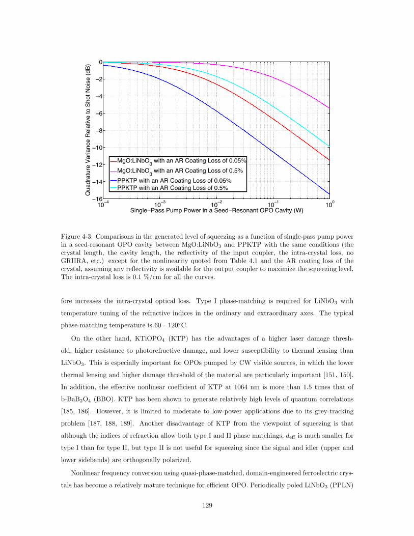
10−4 10−3 10−2 10−1 100−16

−14

−12

−10

−8

−6

−4

−2

0

Single−Pass Pump Power in a Seed−Resonant OPO Cavity (W)

Qua

drat

ure

Varia

nce

Rela

tive

to S

hot N

oise

(dB)

MgO:LiNbO3 with an AR Coating Loss of 0.05%MgO:LiNbO3 with an AR Coating Loss of 0.5%PPKTP with an AR Coating Loss of 0.05%PPKTP with an AR Coating Loss of 0.5%

Figure 4-3: Comparisons in the generated level of squeezing as a function of single-pass pump powerin a seed-resonant OPO cavity between MgO:LiNbO3 and PPKTP with the same conditions (thecrystal length, the cavity length, the reflectivity of the input coupler, the intra-crystal loss, noGRIIRA, etc.) except for the nonlinearity quoted from Table 4.1 and the AR coating loss of thecrystal, assuming any reflectivity is available for the output coupler to maximize the squeezing level.The intra-crystal loss is 0.1 %/cm for all the curves.

fore increases the intra-crystal optical loss. Type I phase-matching is required for LiNbO3 with

temperature tuning of the refractive indices in the ordinary and extraordinary axes. The typical

phase-matching temperature is 60 - 120C.

On the other hand, KTiOPO4 (KTP) has the advantages of a higher laser damage thresh-

old, higher resistance to photorefractive damage, and lower susceptibility to thermal lensing than

LiNbO3. This is especially important for OPOs pumped by CW visible sources, in which the lower

thermal lensing and higher damage threshold of the material are particularly important [151, 150].

In addition, the effective nonlinear coefficient of KTP at 1064 nm is more than 1.5 times that of

b-BaB2O4 (BBO). KTP has been shown to generate relatively high levels of quantum correlations

[185, 186]. However, it is limited to moderate to low-power applications due to its grey-tracking

problem [187, 188, 189]. Another disadvantage of KTP from the viewpoint of squeezing is that

although the indices of refraction allow both type I and II phase matchings, deff is much smaller for

type I than for type II, but type II is not useful for squeezing since the signal and idler (upper and

lower sidebands) are orthogonally polarized.

Nonlinear frequency conversion using quasi-phase-matched, domain-engineered ferroelectric crys-

tals has become a relatively mature technique for efficient OPO. Periodically poled LiNbO3 (PPLN)

129

and LiTaO3 (PPLT) have been the main focus of research for the past several years [175, 180].

However, when pumped by a visible light source, CW OPOs using these materials are significantly

affected by thermal effects originating from the relatively high absorption of the pump. Furthermore,

PPLN and PPLT show strong photorefractive effects that prevent the stable operation of CW OPOs

near room temperature. To reduce these effects, the nonlinear crystals have to be operated at tem-

peratures near above 140 C, which is inconvenient and significantly reduces the wavelength tuning

range obtainable with a single grating period. Therefore, the development and characterization of

new periodically poled materials with low visible absorption and negligible photorefractive effects is

of great relevance.

Recent progress in the electric field poling of flux-grown KTP has made periodically poled KTP

(PPKTP) a very promising candidate. With its high nonlinearity of |deff | % 10.8 pm/V, PPKTP is

an interesting alternative to PPLN and PPLT. The properties of these different kinds of nonlinear

crystals are compared in Table 4.1. PPKTP has already been used in CW resonant second-harmonic

generation (SHG) [180, 181, 150] and OPO [175, 176, 177, 178, 179] at 1064 nm. These experiments

showed high second-harmonic conversion efficiencies and parametric gains. Very recently, PPKTP

has been used in the generation of entangled photons at 1064 nm [182] and bright squeezed light from

a CW SHG also at 1064 nm [183]. In the latter experiment, Andersen and Buchhave observed a noise

reduction of 13 % below the shot noise limit in the generated second-harmonic field. They reported

that this noise reduction is greater than what could be expected using a normal birefringence phase-

matched KTP crystal with the same experimental parameters. Aoki et al. reported the generation

of CW squeezed vacuum at 946 nm using a PPKTP crystal in an OPO and observed a squeezing

level of 5.6±0.1 dB and an anti-squeezing level of 12.7±0.1 dB [138]. Very recently, Suzuki et

al. have observed 7.2±0.2 dB of CW squeezing at 860 nm using a PPKTP crystal in a bow-tie

cavity [139]. Hirano et al. also observed the generation of pulsed squeezed light from a single-pass

degenerate optical parametric amplifier (OPA) pumped by a CW second-harmonic wave using a

PPKTP crystal and reported a squeezing level of 3.2 dB and an anti-squeezing level of 6.0 dB at

1064 nm [184]. These demonstrations of high level squeezing agree with the theoretical prediction

that a considerable amount of squeezing can be generated with large input pump powers and well-

phase-matched interactions [190]. To see the squeezing level gain, Fig. 4-3 compares MgO:LiNbO3

and PPKTP in the generated level of squeezing as a funtion of single-pass pump power in a seed

resonant OPO cavity with the same conditions (the crystal length, the cavity length, the reflectivity

of the input coupler, no GRIIRA, etc.) except for the nonlinearity quoted from Table 4.1, the

intra-crystal loss, and the AR coating loss of the crystal, assuming any reflectivity is available for

the output coupler to maximize the squeezing level. In the figure, we can learn that the separation

in the level of squeezing between MgO:LiNbO3 and PPKTP for different losses changes weakly, and

therefore, even if the crystal or the AR coating on its surfaces is lossy, PPKTP in an OPO cavity

130

gives a gain of about 4 dB compared with MgO:LiNbO3 in the same OPO cavity.

Recent experiments on quasi-phase-matching in gallium arsenide (GaAs), which has a very high

nonlinear coefficient of 69 - 170 pm/V (several to ten times larger than that of PPKTP and PPLN)

and a wide transparency range of 0.7 - 17 µm, make this material very attractive for SHG and OPO

as well as squeezing in the mid-IR range [191, 192]. However, the growth of periodically poled GaAs

structures with sufficient quality and thickness is a delicate issue.

4.3.4 Cavity Configurations

As discussed in Chap. 2, the optical configuration of an OPO cavity needs to be well-designed

to optimize the level of squeezing generated in the OPO. From Eq. (2.69), the generated level of

squeezing is completely determined by the nonlinear coupling efficiency x and the escape efficiency

ηout. Typically, the input coupler is HR-coated. Fig. 4-4 shows the theoretically achievable levels

of squeezing as a function of pump power for various output coupler reflectivities. An input coupler

with a reflectivity of 99.5% and an intra-cavity loss of 0.2% are assumed for the figure.

10−3 10−2 10−1 100 101−16

−14

−12

−10

−8

−6

−4

−2

0

P/Pth

Qua

drat

ure

Varia

nce

Rela

tive

to S

hot N

oise

(dB)

98%94%90%86%

Figure 4-4: The theoretically achievable levels of squeezing as a function of pump power normalizedto the OPO threshold in the case of an output coupling reflectivity of 86% for various outputcoupler reflectivities. The reflectivity of the input coupler and the intra-cavity loss are 99.8% and0.2% respectively.

What we can read from this figure is that if a sufficiently high pump power is available, a

low-reflectivity output coupler should be used to obtain a high level of squeezing. However, if

it is not available, an output coupler with a higher reflectivity should be used since the level of

131

squeezing decays more quickly. In addition, when a high pump power is used, it triggers undesirable

photothermal effects [134], degrading the level of squeezing, although it is not shown in the figure.

This situation also requires a high mode-matching efficiency between the pump and the cavity mode

in the case of a singly-resonant OPO cavity since otherwise, it would cause unnecessary photothermal

noise [134].

4.4 Long-Term Stability

4.4.1 Overview

The third requirement is long-term stability for the practical use of squeezing in the GW detectors

such as LIGO, VIRGO, GEO600, and TAMA300 that typically run for a few years continuously

although there are periods for maintenance from time to time during their science runs. First of

all, the OPO cavity needs to be kept stably locked on resonance to maintain a constant level of

squeezing. In the case of an empty cavity, a bright coherent field is typically used to lock the

cavity on resonance. However, as discussed in Sec. 4.2.2, in the case of the OPO cavity, a bright

field cannot be used as a seed to produce squeezing in the GW detection band, and therefore, an

alternative method is required to maintain vacuum at the fundamental frequency on resonance in

the OPO cavity. Secondly, the phase-matching condition of the OPO needs to remain satisfied. In

type I phase-matching, temperature tuning of the nonlinear crystal via change in refractive index

with temperature, or the so-called dn/dT effect, is used to match the two refractive indices in the

ordinary and extraordinary axes of the nonlinear crystal. In the case of quasi-phase-matching in a

periodically poled nonlinear crystal, temperature tuning of the crystal is also required, but against

thermal expansion. Thus, in all cases, stable temperature control of the crystal is required, which

indicates that a temperature control servo and an oven for the crystal need to be well-designed.

Finally, the interface of squeezing to the interferometer also needs to be stabilized. Otherwise, the

coupling of the anti-squeezed noise that comes with the squeezed noise would degrade the strain

sensitivity of the GW detector. However, since the injected squeezed vacuum field does not contain

any coherent amplitude, the standard scheme to read out the relative phase between the squeezed

vacuum and the interferometer field is not applicable, and therefore, an alternative readout scheme

is necessary.

In summary, the following three requirements need to be satisfied for the stable operation of

squeezing in the GW detectors: (1) stable control of the OPO cavity resonance, (2) stable control

of OPO phase-matching, and (3) stable control of squeezing (the squeeze angle). In the following

sections, these requirements are discussed and a few different techniques are compared. In Chap. 7,

a few ideas about increased stability by cavity-less generation of squeezed states will be presented.

132

4.4.2 Control of OPO Cavity Resonance

Control with a Subcarrier

In many cases, the OPO cavity is a singly resonant cavity in which the cavity mirror reflectivities

form a cavity at the fundamental frequency, but not at the second-harmonic frequency. The second-

harmonic field typically singly or doubly passes through the OPO. In this case, a frequency-shifted

subcarrier can be used to lock the OPO cavity such that a vacuum field at the fundamental frequency

resonates in the OPO cavity. The frequency of the subcarrier can be either one FSR away from the

TEM00 mode in which the vacuum at the fundamental frequency resonates or one of the TEM00

modes near the fundamental vacuum resonance frequency in the orthogonal polarization. The dif-

ference in optical length between the two polarizations is attributed to the birefringent property

of nonlinear crystals (certainly in type I phase-matched crystals, but even in quasi-phase-matched

periodically poled crystals). In the former case, the FSR of a typical OPO cavity is on the order of

GHz due to its short cavity distance, and therefore, it is most likely that a second laser is used to

supply the subcarrier unless a GHz acousto-optic modulator (AOM) is available. In the latter case,

if a TEM00 near the fundamental vacuum resonance frequency is available and its frequency shift is

on the order of 100 MHz, passing some portion of the fundamental field through an AOM singly or

doubly is sufficient to frequency-shift it.

If locking the OPO cavity with a subcarrier is only of interest, both methods work well. However,

if the generated squeezed vacuum field is injected into the interferometer, the second method works

better than the first method in that in the first method, since the frequency-shifted subcarrier is in

the same polarization as the squeezed vacuum field, it is not an easy task to isolate the squeezed

vacuum field from the composite field without attenuating the level of squeezing. One could suggest

an optical cavity to filter out the subcarrier, but mode-matching the squeezed vacuum field to such

a cavity is typically 80% in practice, meaning that 20% of squeezing is lost in the filtering process.

Without filtering, the subcarrier travels along with the squeezed vacuum to the interferometer and

might have an undesirable effect on the interferometer although it could be rejected by the signal-

recycling cavity (SRC) or output mode-cleaner (OMC) in Advanced LIGO, depending on the design

of the cavity resonance frequencies. On the other hand, in the second method, a polarizer can easily

separate the squeezed vacuum from the subcarrier without any significant optical loss and hence,

locking the OPO cavity can be done independently from the interferometer.

Control with a Second-Harmonic Pump

A doubly resonant OPO cavity at both the fundamental and second-harmonic wavelengths has a

few advantages over a singly resonant OPO cavity [115]. One advantage is that the pump power

can be increased by a factor of the cavity finesse, and thus, when the power of the incident second-

133

harmonic field is insufficient, this is a good strategy. As discussed in Sec. 4.3.4, in principle, the

more pump power is available, the higher the achievable level of squeezing is. However, since the

nonlinear crystal absorbs some amount of the pump power, the pump with a higher power makes

the cavity thermally unstable. Another advantage is that the mode coupling of the pump to the seed

is perfect in the doubly resonant OPO cavity compared to the singly resonant OPO cavity because

the cavity selects the resonating mode. This is an efficient pumping process in that no pump power

is wasted in the OPO cavity. One disadvantage is that vacuum at the fundamental frequency might

not resonate exactly due to the difference in optical travel distance between the fundamental and

second-harmonic frequencies. In type I phase-matching, their refractive indices are equivalent under

the condition that the phase-matching condition is satisfied. In quasi-phase-matching, a tunable

phase compensation plate that compensates for the phase difference between the two frequencies is

required, but it might be lossy in the cavity.

4.4.3 Control of OPO Phase Matching

In type I phase matching, the dependence of the refractive index of a nonlinear crystal on its

temperature or the so-called dn/dT effect is used to match the refractive indices of the material in

the ordinary and extraordinary axes. As mentioned in Sec. 2.4.4, in the case of LiNbO3, dno/dT =

3.3 × 10−6 K−1 in the ordinary axis and dne/dT = 37 × 10−6 K−1 in the extraordinary axis, both

at λ = 1.0 - 4.0 µm. These are fairly large values for temperature change on the order of 10 mK.

As shown in Fig. 2-7, the strength of nonlinear interaction in both SHG and OPO cavities strongly

depends on the temperature of the nonlinear crystals, and therefore, temperature fluctuations in the

crystals are directly coupled to nonlinearity fluctuations, that is, fluctuations in the generated level

of squeezing. In addition, as the size of the crystal increases, the effective temperature range gets

narrower. The typical size of nonlinear crystals is about 6 mm, and therefore, the effective FWHM

temperature range is 0.5 K.

On the other hand, periodically poled nonlinear crystals do not require temperature-tuning of

their refractive indices for phase-matching. The only requirement for temperature control is to

maintain the grating period against thermal expansion. The typical FWHM temperature range of

PPKTP at 1064 nm is 5 K, which is about 10 times larger than that of LiNbO3 in type I phase-

matching. Another advantage of the large temperature range of PPKTP is that it significantly

reduces difficulties in fabrication of ovens for temperature control that would be needed for type I

phase-matching. In this respect, periodically poled nonlinear crystals such as PPKTP are better in

stability against fluctuations in phase-matching than nonlinear crystals that require type I phase-

matching such as LiNbO3.

134

4.4.4 Control of Squeezing

Overview

In Sec. 2.7, two methods of controlling squeezed vacuum fields without a carrier field have been

described. However, while these techniques are useful in stand-alone squeezers, the validity of the

techniques for the injection and control of a squeezed vacuum field in a laser-interferometric GW

detector needs to be investigated. In this section, practical issues and solutions are discussed.

Quantum Noise Locking

The quantum noise locking technique is useful in any optical system since it does not require any

coherent sidebands (although there are vacuum sidebands that are generated by modulating the

squeeze angle of the squeezed vacuum field). The only requirement is that the length sensing

detector of an interferometer is required to detect its quantum noise that is demodulated to obtain

an error signal for noise-locking the squeeze angle. Because of the absence of any coherent sidebands,

the level of shot noise that is equal to the quadrature sum of all the fields incident on the length

sensing photodetector does not change. One disadvantage is its low stability (both long-term and

short-term). Since the noise-locking error signal relies on the noise on the noise or kurtosis, its

variance strongly couples to the stability of the noise-locking. Therefore, as shown in Eqs. (2.152)

and (2.153), unless the generated level of squeezing is very large, the stability of the noise-locking

cannot be better than the stability of the coherent control method.

Advantages

• Does not require any coherent sidebands• Does not require any frequency filters or photodetectors• Requires only the length sensing detector to measure the quantum noise of an interferometer

Disadvantages

• Low stability• Lower achievable level of squeezing

Table 4.2: Advantages and disadvantages of the quantum noise locking technique.

Coherent Control of Squeezing

The coherent control method has the obvious advantage over the quantum noise locking method

that its stability is much higher, indicating that the maximum achievable level of squeezing is higher

[138]. On the other hand, it has one serious disadvantage that the coherent signal and idler fields

co-propagate with the squeezed vacuum field. In the DC readout scheme of Advanced LIGO as

shown in Fig. 4-5, all RF sidebands are removed by the OMC before measuring the carrier field

with the length sensing photodetector. The purpose of the OMC is to remove RF sidebands that

135

are not filtered by the arm cavities of the interferometer and clean the mode of the interferometer

carrier field, and therefore, the signal and idler fields should not transmit through the OMC since

they would otherwise contaminate the carrier field that possible GW signals would beat with. In

this respect, an error signal for the coherent control needs to be obtained from the beat between

the signal/idler and interferometer RF sidebands (not the interferometer carrier) at the rejection

port of the OMC. One could suggest putting a pickoff mirror in between the optical circulator and

OMC, but it should be suspended not to pick up any ground and mechanical noise, assuming that

the OMC is suspended for the same reason.

If these issues can be overcome, the coherent control technique should be used in the imple-

mentation of squeezing in next generation GW detectors such as Advanced LIGO since its control

stability can simply be enhanced by increasing the gain of the servo.

LASER

SqueezedVacuum

OpticalCirculator

Photodetector

Fabry-PerotMichelson

PowerRecycling

Mirror

Signal RecyclingMirror

InputMode

Cleaner

OutputMode

Cleaner

Photodetector

Figure 4-5: The optical configuration and readout scheme of Advanced LIGO. Another filter cavitycalled the output mode cleaner (OMC) is planned to be added to the interferometer output toremove any RF sidebands and clean the mode of the carrier field.

4.5 Frequency-Dependent Squeezing

4.5.1 Introduction

The fourth requirement is frequency-dependent squeezing. In Chap. 1, two limiting quantum noise

sources in GW detectors have been addressed. They are photon shot noise at high frequencies

136

Advantages

• High stability• Higher achievable level of squeezing• Easy to control

Disadvantages

• Requires RF sidebands• Requires a complicated optical setup to generate and detect correlated signal and idler fields• Requires a filter cavity that filters out the RF sidebands before the length sensingphotodetector• Requires the beat between the signal/idler and RF sidebands (not the carrier field) from theinterferometer to obtain an error signal for the coherent control

Table 4.3: Advantages and disadvantages of the coherent control method.

that arises from uncertainty due to quantum mechanical fluctuations in the number of photons

at the interferometer output and quantum radiation pressure noise at low frequencies that arises

from mirror displacements induced by quantum radiation pressure fluctuations [82, 83]. As in Eqs.

(1.61) and (1.66), in a simple Michelson interferometer, the strain associated with the shot noise is

proportional to 1/√

Pin while the strain associated with the radiation pressure noise is proportional

to√

Pin. Thus, increasing the laser power improves the strain sensitivity by reducing the shot noise

while degrading it by increasing the radiation pressure noise, or vice versa.

The effect of the radiation pressure noise is to ponderomotively squeeze the optical fields with a

frequency dependent squeeze angle due to the frequency dependent response of the test masses [82].

This presents difficulty in injecting squeezed states into the interferometer because the squeeze angle

of the squeezed state source must be matched to the ponderomotive squeeze angle. Squeezing with a

frequency-independent or constant squeeze angle improves the sensitivity at some frequencies in the

GW detection band, but degrades it at other frequencies due to the orthogonality of amplitude and

phase quadratures corresponding to radiation pressure noise and shot noise in the GW detectors.

For a conventional GW detector with arm lengths L and mirror masses m, the quantum noise in

the GW strain signal when a squeezed field a with squeeze factor r and squeeze angle θ is injected

into the dark port of the interferometer is given by [82, 193]

h(Ω) = hSQL

√

1 + K2

2K

[

Va1 sin2 (θ + Φ) + Va2 cos2 (θ + Φ)]

, (4.1)

where hSQL is given by Eq. (1.70), Ω is the sideband (measurement) frequency, K is the effective

coupling constant given by Eq. (1.71), Va1 and Va2 are the amplitude and phase quadrature variances

of the input squeezed field, and Φ = cot−1 K is the phase gained by the sideband frequency Ω while

traveling one way in the SRC4. Fig. 4-6 shows quantum noise and squeezed quantum noise with

4In other words, it is the effective ponderomotive squeeze angle of the interferometer.

137

101 102 103 10410−24

10−23

10−22

10−21

Frequency (Hz)

Stra

in (H

z−1/

2 )

Unsqueezed Quantum NoisePhase−Squeezed Quantum NoiseAmplitude−Squeezed Quantum Noise

Figure 4-6: The comparison of the unsqueezed quantum noise and the squeezed quantum noise withfrequency-independent squeeze angles in a conventional GW detector with parameters m = 30 kg,L = 4 km, λ = 1064 nm, γ/(2π) = 100 Hz, P = PSQL, and a squeeze factor of r = 2. Squeezingwith a constant squeeze angle reduces the quantum noise at high frequencies while increasing it atlow frequencies, or vice versa. Phase-squeezing and amplitude-squeezing correspond to θ = 0 andθ = π/2 respectively.

a constant (frequency-independent) squeeze angle in a conventional GW detector. Squeezing with

a constant squeeze angle reduces the quantum noise at high frequencies while increasing it at low

frequencies, or vice versa. Squeezing with squeeze angle θ = −Φ reduces the quantum noise at all

frequencies.

Squeezed states generated by OPOs are generally frequency-independent, but the desired angle

may be produced by using optical filters placed between the squeezed state source and the interfer-

ometer so that broadband squeezing can be achieved in the GW detection band. A few different

filtering schemes have been proposed: (1) optical cavities with narrow linewidths comparable to the

bandwidth of the interferometer (100 Hz) [82, 104], (2) filters by use of electromagnetically induced

transparency (EIT) [193], and (3) filters for squeeze amplitude attenuation [194]. The properties

and practicality of these filters are discussed in the following sections.

4.5.2 Cavities with Narrow Linewidths

A scheme that uses a pair of successive lossless Fabry-Perot filter cavities as a frequency-dependent

squeeze angle filter has been proposed [82], and the proof of principle has been experimentally

demonstrated at MHz frequencies [159]. When an input squeezed field is incident on a cavity which

138

is not impedance-matched and the carrier frequency and cavity resonance frequency are equal, its

sidebands obtain frequency-dependent phase shifts when the field reflects back. Since squeezing is

the sum of the quantum sidebands centered around the carrier frequency, the sum of those quantum

sidebands with frequency-dependent phase shifts yields frequency-dependent squeezing.

The two filter cavities (denoted I and II) produce phase shifts θI± and θII± on the sidebands at

frequencies ±Ω. The net phase shifts acquired by the two cavities are given by θ± = θI± + θII±.

Assuming that the carrier frequency of the squeezed field is equal to the resonant frequency of the

cavities, the phase shifts are given by

θI± = tan

(

±Ω

γI

)

, θII± = tan

(

±Ω

γII

)

, (4.2)

where γI and γII are the HWHM linewidths of the cavities. The detail calculations of the squeeze

angle rotation will be given in Sec. 5.2.2.

The biggest problem of this type of filter cavities is that the cavity filters, while producing the

desired squeeze angle, are difficult to build because they require cavities with narrow linewidths

comparable to the bandwidth of the interferometer (100 Hz), which require either km-scale cavities

or high-finesse cavities. For squeeze-angle rotation, high-finesse cavities are somewhat undesirable

due to high optical losses. For example, assuming a round-trip optical loss of 20 × 10−6, a cavity

would have to be nearly 100 m to maintain an effective loss of 10% or less.

4.5.3 Filters by Use of Electromagnetically Induced Transparency

Overview

Alternative filter designs based on EIT media have been proposed [193]. Several properties of

EIT media make them a potentially advantageous alternative to ultra low-loss or km-scale optical

cavities. First, EIT media typically have narrow transmission resonance linewidths. The narrowest

linewidth reported is 1.3 Hz in a paraffin coated cell with 85Rb as the EIT medium [195]. The

EIT media can also be very compact, with typical lengths of ∼ 10 cm. Second, the resonance

linewidth may be adjusted in non-invasive ways, by changing the atomic density [196] or drive field

intensity [197], to optimize the filtering. Altering the linewidth of an optical cavity, on the other

hand, usually requires changing the transmission of the mirrors or the macroscopic cavity length.

Other variable reflectivity techniques such as three-mirror cavities are possible, but issues of fringe

control, scattered light and mode mismatch are compounded in such systems. Third, EIT media

can be nearly 100% transmissive for the probe field [198, 199]. Fourth, mode matching of the spatial

mode of the squeezed (probe) beam to that of the EIT is not critical, as it is for an optical cavity,

where mode mismatch can be a significant source of optical loss [198]. Fifth, EIT media have also

been shown to preserve squeezed states in transmission [200, 201]. These reasons lead naturally to

139

ωbc

ωd

ω-Ω

ω+Ω

ω

∆

δΩ

Ω

|a⟩

|b⟩

|c⟩

LASER

SQZ

EIT

OpticalCirculator

Photodetector

MichelsonInterferometer

Pickoff

SqueezedVacuum

Figure 4-7: Left : A generic three-level EIT system. The susceptibility of the EIT medium, χ, isa function of the frequency of the probe field, ω, the sideband frequency, Ω (relative to the carrierfrequency of the probe, ω), the frequency of the ground state splitting, ωbc, the two-photon detuningof the probe field, δ = ω − ωd − ωbc, the one-photon detuning of the drive field, ∆, and the lengthof the EIT medium, l. Right : A proposed configuration for a squeeze EIT filter and GW detector,where SQZ: squeezed field generator, EIT: EIT filter.

consideration of using EIT for squeezed state filters.

Theory of Squeeze Amplitude Attenuation and Squeeze Angle Rotation by EIT

The energy level scheme for one photon resonant EIT is shown in Fig. 4-7. Using the parameters

defined in Fig. 4-7, the EIT transmission as a function of the sideband frequency, Ω, is given by

T (ω + Ω) = exp

(

i

∫ l

0keit(ω + Ω, z) dz

)

, (4.3)

where keit is the wavevector of the probe field through the EIT medium. For most cases, it is

reasonable to assume that the susceptibility of the medium |χ(ω + Ω, z)| + 1 and Ω + ω, then the

wavevector can be written as

keit(ω + Ω, z) =ω + Ω

c

√

1 + χ(ω + Ω, z) % ω

c

(

1 +χ(Ω, z)

2

)

. (4.4)

In the frequency domain defined by Eq. (1.60), substituting Eq. (4.4) into Eq. (4.3) and moving

into the rotating frame of the probe field a with frequency ω [131], we find the EIT transmission at

sideband frequencies ±Ω,

T (±Ω) = T±eiΘ± , (4.5)

140

where

T± ≡ exp

(

− ω

2c

∫ l

0χ2(±Ω, z) dz

)

, (4.6)

Θ± ≡ ω

2c

∫ l

0χ1(±Ω, z)dz. (4.7)

Here χ1(Ω, z) and χ2(Ω, z) are the real and imaginary parts of χ(Ω, z), respectively. χ1(Ω, z) is

responsible for phase shift and χ2(Ω, z) is responsible for signal strength attenuation.

When the input field a is injected into an EIT medium, the output field b and its adjoint b† are

given in terms of a and its adjoint a† by

b(Ω) = T (Ω)a(Ω) + L+(Ω)v(Ω), (4.8)

b†(−Ω) = T ∗(−Ω)a†(−Ω) + L∗−(−Ω)v†(−Ω), (4.9)

where L± is the EIT absorption coefficient such that

L± =√

1 − T 2± (4.10)

and v is a vacuum field coupled in by the absorption loss. a(Ω) and a†(−Ω) satisfy the commutation

relations[

a(±Ω), a†(±Ω′)]

= 2πδ(Ω − Ω′

), (4.11)

and all others vanish [similarly for v(Ω) and v†(−Ω)]. Using the definitions of the amplitude and

phase quadratures in Eqs. (2.10) and (2.11), we find the quadrature field amplitudes of the output,

in a compact matrix form, to be

b = Ma +√

1 −(

A2+ + A2

−)

vs, (4.12)

where we use the two-photon matrix representation

a ≡

a1

a2

(4.13)

for the operator, a (and similarly for b and v), and

M = eiϕ−

cosϕ+ − sinϕ+

sinϕ+ cosϕ+

A+ iA−

−iA− A+

(4.14)

is a matrix representing propagation through the EIT medium. M comprises an overall phase shift,

141

ϕ−, rotation by angle, ϕ+, and attenuation by a factor, A+. Here we have defined

ϕ± ≡ 1

2(Θ+ ± Θ−) , A± ≡ 1

2(T+ ± T−) , (4.15)

and performed a unitary transformation on v, such that

√

1 −(

A2+ + A2

−)

vs =1

2

L+ + L− i (L+ − L−)

−i (L+ − L−) L+ + L−

v (4.16)

and vs behaves as ordinary unsqueezed vacuum. For symmetrical lineshapes with respect to the

carrier, χ1(Ω) = −χ1(−Ω), and ϕ+ therefore vanishes, giving no quadrature angle rotation, but

attenuating the signal strength. For asymmetrical lineshapes, nonzero ϕ+ gives quadrature angle

rotation.

Application to GW Detectors

Assuming no losses other than those associated with the EIT filter, a squeezed field b with squeeze

factor r and squeeze angle θ = θ0 + ϕ+ is injected into the antisymmetric port of the GW detector

through the EIT filter as shown in Fig. 4-7. The input angle θ0 may be arbitrarily chosen by

microscopic variations in the distance between the squeezed state source and the interferometer.

Following Eq. (4.1), the spectral density of the noise at the output of the GW detector is given by

S(Ω) =h2

SQL

2

(

K +1

K

)

[

V+ sin2 (θ + Φ) + V− cos2 (θ + Φ)]

, (4.17)

where the noise in the anti-squeezed and squeezed quadratures, V+ and V−, respectively, is given by

V+

V−

=

A2+ A2

−

A2− A2

+

e+2r

e−2r

+

1 −(

A2+ + A2

−)

1 −(

A2+ + A2

−)

. (4.18)

EIT Filter Overview

The following three kinds of EIT filters are proposed: (i) low-pass, band-pass, and high-pass squeeze

amplitude attenuation filters, (ii) an S-shaped filter as a frequency-dependent squeeze angle rotator,

and (iii) an intra-cavity EIT filter as a frequency-dependent squeeze angle rotator.

To obtain expressions for the EIT transmission T (±Ω), it is useful to use the formulas for EIT

susceptibility χ [202, 203]

ω

2 c

∫ l

0χ1(±Ω, z) dz = A(∆)

Γ(δ ± Ω)

Γ2 + (δ ± Ω)2+ B(∆)

Γ2

Γ2 + (δ ± Ω)2, (4.19)

ω

2 c

∫ l

0χ2(±Ω, z)dz = A(∆)

Γ2

Γ2 + (δ ± Ω)2+ B(∆)

Γ(δ ± Ω)

Γ2 + (δ ± Ω)2+ C(∆), (4.20)

142

10 100 10000.1

1.0

10

Frequency [Hz]

S h / S h(U

nsqu

eeze

d)

a2 squeezed a1 squeezed

Band pass Optimal rotation/intra−cavity EIT

S resonance, low absorption S resonance, high absorption

Low pass

High pass

Figure 4-8: The noise spectral density of a GW detector, normalized to the noise density with nosqueezed state injection. We show the effect of low-pass (red), band-pass (green), high-pass (cyan),S-shaped (blue for low and brown for high absorption levels), and intra-cavity (black) filters andcompare it to frequency independent schemes. The dashed curves show unfiltered squeezing of thea1 (green) and a2 (red) quadratures.

where Γ is the EIT resonance linewidth and the coefficients A, B and C depend on the intensity and

detuning, ∆, of the drive field. The first term on the right hand side in Eq. (4.19) corresponds to

asymmetric phase dependence on the two-photon detuning δ±Ω and the second term is responsible

for symmetrical Lorentzian dependence. Similarly, the first term in Eq. (4.20) corresponds to

symmetrical dependence on the absorption coefficient of the EIT medium, the second term indicates

asymmetric absorption, and the third term corresponds to broadband absorption in the medium.

Inserting Eqs. (4.19) and (4.20) into Eqs. (4.6) and (4.7) respectively, we get explicit expressions

for T± and θ±, which are used to calculate the noise at the output of the GW interferometer S(Ω),

as described in Sec. 4.5.3.

Squeeze Amplitude Attenuation Filters

If we take A = −C, B = 0, C ≥ 10, and δ = 0 [197], then ω2c

∫ l0 χ2(±Ω, z)dz ≥ 10 for Ω ) Γ and

ω2c

∫ l0 χ2(±Ω, z)dz % 0 for Ω + Γ, and we obtain a symmetric EIT transmission line with A− = 0

and ϕ+ = 0. This can be used as a squeeze amplitude filter that retains squeezing at low frequencies,

but causes ordinary (unsqueezed) vacuum to replace the anti-squeezed noise at higher frequencies

that are outside the EIT bandwidth. This is equivalent to the low-pass filters proposed in Ref.

[194]. Similarly, buffer-gas-induced electromagnetically induced absorption (BGIEIA) [202] may be

used as a high-pass filter. BGIEIA is similar to EIT, with a narrowband absorption resonance

143

instead of the transmission resonance of EIT. High-pass filtering with BGIEIA can be realized with

parameters A ≥ 10, B = 0, C = 0, and δ = 0, such that ω2c

∫ l0 χ2(±Ω, z)dz % 0 for Ω ) Γ and

ω2c

∫ l0 χ2(±Ω, z)dz ≥ 10 for Ω + Γ. A combination of two EIT resonances, equally detuned from the

carrier (obtained by Zeeman splitting [204]), serves as a band-pass filter. In Fig. 4-8 the effect of low-

pass, band-pass, and high-pass EIT filters on the noise spectral density of a GW detector are shown.

The noise spectra are normalized by the noise spectral density of a conventional interferometer with

no squeezed state injection, which corresponds to the unity in Fig. 4-8. In each case, the harmful

effects of squeezing with a constant squeeze angle are reduced.

Squeeze Angle Rotation Filters

In principle, optimum squeeze angle rotation, corresponding to θ % −Φ, can be obtained with an

asymmetrical or S-shaped EIT filter, realized under conditions similar to BGIEIA with parameters

A % 0, B = −π/2, and C > |B|. In this case, the noise spectral density can be optimized over most

frequencies. However, as is evident from the curves labeled S resonance in Fig. 4-8, the improvement

is small because of the high off-resonance losses associated with the coefficient C. Optimization would

require setting C = 0. The noise is decreased at both high and low frequencies, but worsened in

the middle of the band due to two effect. First, the imbalance in absorption (A− 0= 0) between the

upper and lower sidebands required to obtain the squeeze angle rotation causes the quadratures to

be mixed and the noise may be higher than shot noise. Second, the imperfect squeeze angle rotation,

θ % −Φ, couples in noise from the anti-squeezed quadrature.

Placing an EIT medium in an optical cavity narrows the cavity linewidth [205, 206]. We consider

a symmetric EIT transmission resonance, such as the one used for our low-pass filter, with a large

linewidth Γ % 10 kHz, such that T± % 1, ϕ+ % 0, and ϕ− % ±ωl2cΩ

dχ1

dΩ

∣

∣

∣

Ω=0in the frequency band of

interest (100Hz). This configuration may be understood in terms of the group velocity of the light

through the EIT medium

vg =c

ω

(

dχ1

dΩ

∣

∣

∣

∣

0

)−1

. (4.21)

We may then express

ϕ− % l

2vgΩ =

Ωlec

, (4.22)

where le = c2vg

l is the effective cavity length. The EIT medium serves as an additional delay line

inside the cavity. A group velocity as low as 8 m/s in a 12 cm long Rb vapor cell was demonstrated

by Budker et al. [195], giving an effective length on the order of 106 m. To use an intra-cavity EIT

medium as a squeeze angle rotation filter, we must detune the cavity (but not the EIT medium)

from the carrier. For this case, the rotation arises from the detuned cavity, similar to the filters

in Ref. [82], and not from the EIT. The EIT acts only to modify the resonant linewidth of the

144

cavity by increasing its effective length. To achieve the required 100 Hz linewidth for the filter,

we use an EIT with a large effective length, combined with a short cavity. The performance of

this cavity is essentially identical to that of an isolated cavity with no EIT and length equal to le,

and may achieve optimal squeeze angle rotation with a much smaller optical loss than a traditional

cavity of the same linewidth with the same real (not effective) length, giving improved GW detector

sensitivity at all frequencies. We note that T± % 1 is a reasonable approximation because of the

narrowed linewidth of the system (Ti vg/l + Γ, where Ti is the transmission of the cavity input

mirror). Detailed calculations show that the effective loss of the system may even be reduced by

placing the EIT in a shorter cavity for some parameter choices. The broadband reduction of noise

from such an intra-cavity EIT filter is shown in Fig. 4-8, and corresponds exactly to the much

coveted optimal frequency-dependent squeezing of Ref [82].

4.5.4 Filters for Squeeze Amplitude Attenuation

Introduction

Although frequency-dependent squeezing can be performed by an EIT filter that has advantages

over other filter designs in optical losses, compactness, and the tunability of the filter linewidth, an

EIT medium for the laser wavelength used in the existing or future GW detectors such as LIGO and

Advanced LIGO (1064 nm) is unavailable.

To avoid the harmful effects of squeezing with a constant squeeze angle and the need for a low-loss

or high-finesse cavity, another kind of filter cavities that behaves as a high-pass filter for the squeeze

amplitude instead of giving a frequency-dependent squeeze angle has been proposed [194]. These

filters operate on the principle that the squeezed state with a frequency-independent squeeze angle

has beneficial effects over some frequency band, but harmful effects over other frequency bands, and

those harmful effects can be mitigated by introducing a frequency-dependent optical loss.

When a squeezed vacuum field with a constant squeeze angle is injected into an impedance-

matched optical cavity, it is entirely reflected by the filter cavity outside of the cavity linewidth

whereas within the linewidth it is entirely transmitted and replaced by a vacuum field that cou-

ples in due to the cavity transmission and intra-cavity losses of the squeezed vacuum field. When

this squeeze amplitude filter is applied to a squeezed vacuum field before being injected into GW

detectors, the interferometer shot noise can be reduced by squeezing at high frequencies while anti-

squeezing is attenuated at low frequencies, giving a semi-broadband reduction of the quantum noise.

In this section, such a squeeze amplitude high-pass filter is theoretically described and then

experimentally demonstrated by measuring the reflection of a squeezed vacuum field from the filter

cavity. It is found that cavity detunings play an important role in the performance of the high-pass

filtering effect.

145

Theory

Consider a squeezed vacuum field [a = (a1, a2)T ] with a constant squeeze angle injected into a

filter cavity with input mirror reflectance r1 and transmittance t1, output mirror reflectance r2, and

intra-cavity mirror reflectance r3 that accounts for intra-cavity losses, as shown in Fig. 4-9. Then,

moving into the rotating frame of the carrier field, the reflection from the filter cavity b is given in

the frequency domain defined in Eq. (1.60) by

b1 = ρ(Ω)a1 +√

1 − |ρ(Ω)|2v1, b2 = ρ(Ω)a2 +√

1 − |ρ(Ω)|2v2, (4.23)

where ρ is the cavity reflection coefficient given by

ρ(Ω) = r1 −t21r2r3e−2iΩLAF/c

1 − r1r2r3e−2iΩLAF/c, (4.24)

and v = (v1, v2)T is the vacuum field that couples with the reflection due to the transmission and

intra-cavity loss of the input squeezed vacuum field. Here LAF is the half-length of the amplitude

filter cavity.

r1, t2

a

b

Loss-AssociatedVacuum Mode

r3, t3Intra-CavityLoss

r2, t2 Transmission-AssociatedVacuum Mode

Figure 4-9: A schematic of a squeeze amplitude filter cavity that consists of input mirror reflectancer1 and transmittance t1, output mirror reflectance r2, and intra-cavity mirror reflectance r3 thataccounts for intra-cavity losses.

The mathematical description of the filter is similar to that of the EIT filter that has been given

in Sec. 4.5.3, except that in the case of the squeeze amplitude filter, the linewidth of the filter cavity

is symmetric and the center frequency of the input squeezed vacuum field is equal to the resonance

frequency of the filter cavity (or not detuned from it). The quadrature variances of the reflection is

146

then given by

Vb1(Ω) = |ρ(Ω)|2Va1 + 1 − |ρ(Ω)|2, Vb2(Ω) = |ρ(Ω)|2Va2 + 1 − |ρ(Ω)|2, (4.25)

where we have used Vv1 = Vv2 = 1. At frequencies below the linewidth of the filter, the squeezed

vacuum field transmits through the filter cavity, whereas at frequencies above the linewidth, the field

reflects back by the cavity, and therefore, the filter cavity behaves as a squeeze amplitude high-pass

filter.

Experiment

To demonstrate the squeeze amplitude filtering effect at a wavelength of 1064 nm, a squeezed vacuum

field is prepared using a sub-threshold OPO. Since it is known that squeezed fields generated by

light-seeded OPO cavities have squeezing only at MHz frequencies, a vacuum field is used as a

seed to the OPO. The OPO (different from the OPO in Chap. 3) that consists of a hemilithic

7%MgO:LiNbO3 crystal and an output coupling mirror is pumped by 600 mW of a second-harmonic

field at 532 nm. Type I phase-matching is used to satisfy the OPO phase-matching condition. The

FSR and FWHM linewidth of the OPO cavity at 1064 nm are 362.1 MHz and 2.0 MHz respectively.

The second-harmonic pump doubly passes through the OPO5. The cavity is locked using the Pound-

Drever-Hall (PDH) locking techcnique with a frequency-shifted subcarrier field. The OPO crystal

is temperature-controlled at the phase-matching temperature of 72.1C to maximize the nonlinear

interaction between the seed and pump fields.

The generated squeezed vacuum field is injected into a test filter cavity that consists of three

mirrors with a FWHM linewidth of 856 kHz and a FSR of 713 MHz. The triangular geometry is

chosen such that the reflected field can be geometrically isolated from the injected field. The filter

cavity is locked with a coherent light injected into the cavity from its back so that the reflected

squeezed vacuum field and control field do not propagate in the same direction. A Faraday isolator

is used to remove the control field from coupling into the OPO cavity. To ensure a higher isolation

efficiency, the control field is frequency-shifted relative to the center frequency of the squeezed

vacuum field. The frequency of the control field is carefully tuned so that the center frequency

of the squeezed vacuum field matches the resonance frequency of the filter cavity. The filtered

squeezed vacuum field is measured by a homodyne detector that consists of a 50/50 beamsplitter

and a pair of photodiodes with matched quantum efficiencies of 90%. The difference photocurrent

of the photodetectors is measured by an HP4195A spectrum analyzer (Hewlett-Packard) to measure

the effect of the filter cavity on both squeezed and anti-squeezed shot noise spectra.

The experimental result is shown in Fig. 4-10. The cutoff of the squeezed and anti-squeezed

5Thus, the OPO is not a cavity at 532 nm

147

0.4 0.6 0.8 1 1.2 1.4 1.6 1.8 2

−1

0

1

2

3

4

5

6

7

8

Frequency (MHz)

Qua

drat

ure

Varia

nce

Rela

tive

to S

hot N

oise

(dB)

Unfiltered Squeezed Shot Noise

Unfiltered Anti−squeezedShot Noise

Filtered Squeezed Shot Noise

Filtered Anti−squeezedShot Noise

Figure 4-10: The spectra of squeezed and anti-squeezed quadrature variances which are both filteredand unfiltered by the squeeze amplitude filter. The harmful effect of the anti-squeezing is attenuatedby the filter cavity. The measured spectra are also compared with the theoretical model (solidcurves).

shot noise spectra at about 1 MHz is due to the OPO cavity linewidth. The high-pass filtering

effect of the filter cavity on the squeezed and anti-squeezed shot noise spectra is present in the

mid-band. The peaks at 1.23 MHz are due to the modulation of the OPO crystal for the PDH-

locking technique. The cavity resonance frequency is slightly detuned from the center frequency of

the squeezed vacuum field, such that the cross-coupling of the squeezed and anti-squeezed shot noise

spectra is present (similar to the detuning effect in Sec. 4.5.3). Taking this effect into consideration,

theoretical predictions with the filter cavity mode-matching efficiency ηm and cavity detuning ωd as

free parameters are also shown in Fig. 4-10. They are found to ηm = 0.79 and ωd/(2π) = 320 kHz.

148

Chapter 5

Theory of Quantum Enhanced

Gravitational Wave Detectors

5.1 Overview

In Sec. 1.5, it has been briefly mentioned that the sensitivity of quantum-noise-limited laser inter-

ferometers for precision measurements such as gravitational wave (GW) detectors can be improved

by the injection of squeezed states of light [8, 9] into the antisymmetric port of the interferometers

[10, 207]. The proposed squeezing injection scheme and the effect of squeezing on the sensitivity of

a Michelson interferometer (with a proper frequency-dependent squeeze angle) have been shown in

Fig. 1-6 and 1-7. The effect of squeezing on Advanced LIGO (with a proper frequency-dependent

squeeze angle) has been shown in Fig. 1-8.

In the quantum optical picture, the injection of an optical field in a squeezed state into the

antisymmetric port of the interferometer is equivalent to the replacement of a vacuum (uncorrelated)

field that couples into the port by a correlated field, or in other words, the replacement of an

uncorrelated vacuum field with a correlated (squeezed) field. Since an interferometer is essentially

a two-photon device [82, 103, 96, 104, 102, 20, 19] and a squeezer is a two-photon correlator that

correlates upper and lower quantum sidebands centered around the carrier frequency, the most

proper explanation of the propagation of a squeezed state in the interferometer and its interaction

with the interferometer field is given by the two-photon formalism [19, 20]. In other words, quantum-

enhancement in the interferometer is equivalent to inserting a two-photon correlator (an OPO in

our case) in the path of two uncorrelated photons (vacuum) that couple into the antisymmetric port

of the interferometer as shown in Fig. 5-1.

In this chapter, a basic theory of the propagation of a squeezed vacuum field in an interferom-

eter and its interaction with the interferometer field using the two-photon formalism is described.

149

LASER

OpticalCirculator

Photodetector

Two-PhotonCorrelator

ω+Ω

ω-Ω

LASER

OpticalCirculator

Photodetector

Two-PhotonCorrelator

ω+Ω

ω-Ω

ω+Ω

ω-Ω

UncorrelatedPhotons

UncorrelatedPhotons

CorrelatedPhotons

Michelson Michelson

Figure 5-1: A model of a Michelson interferometer with a two-photon correlator inserted in the pathof two vacuum (uncorrelated) photons that enter the antisymmetric port of the interferometer. Thetwo-photon correlator or an OPO correlates the two input uncorrelated photons, and the output istwo correlated photons (squeezed vacuum).

A signal-recycled Michelson interferometer (SRMI) is used as a model to understand quantum-

enhancement since it is a relatively simple interferometer configuration, but similar to the configura-

tion of Advanced LIGO. The SRMI configuration will be used in the next chapter to experimentally

demonstrate quantum-enhancement. The effect of squeezing on more complex interferometers is

best understood using computer simulations [103].

5.2 Theory of a Quantum-Enhanced Signal-Recycled Michel-

son Interferometer

5.2.1 Equivalent Optical Model

Overview

The interferometer configurations that are used in the currently operational GW detectors such as

LIGO, VIRGO, GEO, and TAMA and envisioned for Advanced LIGO are very complex. Therefore, it

is difficult to understand how a squeezed vacuum field that enters the antisymmetric port propagates

in such a complex interferometer, interacts with the interferometer field, and reduces its quantum

noise. Thevenin’s equivalent optical circuitry is the optical version of Thevenin’s theorem that

any combination of voltage sources, current sources, and resistors with two terminals is electrically

equivalent to a single voltage source and a single series resistor. Using this theorem, the complex

interferometer components which are all linear media can be simplified to simple optical elements.

In this section, the optical equivalent model of a SRMI detector is studied since it is a relatively

150

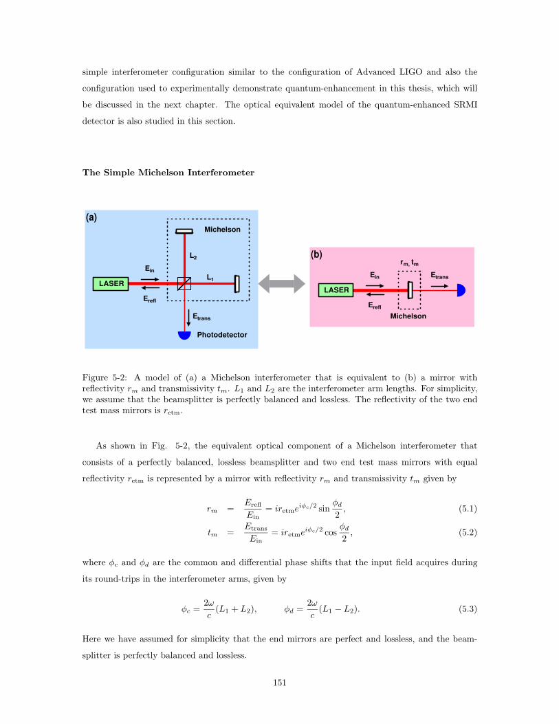
simple interferometer configuration similar to the configuration of Advanced LIGO and also the

configuration used to experimentally demonstrate quantum-enhancement in this thesis, which will

be discussed in the next chapter. The optical equivalent model of the quantum-enhanced SRMI

detector is also studied in this section.

The Simple Michelson Interferometer

(b)

(a)

Ein

L1LASER

Erefl

Etrans

L2

Ein

LASER

Erefl

Etrans

rm, tm

Michelson

Michelson

Photodetector

Figure 5-2: A model of (a) a Michelson interferometer that is equivalent to (b) a mirror withreflectivity rm and transmissivity tm. L1 and L2 are the interferometer arm lengths. For simplicity,we assume that the beamsplitter is perfectly balanced and lossless. The reflectivity of the two endtest mass mirrors is retm.

As shown in Fig. 5-2, the equivalent optical component of a Michelson interferometer that

consists of a perfectly balanced, lossless beamsplitter and two end test mass mirrors with equal

reflectivity retm is represented by a mirror with reflectivity rm and transmissivity tm given by

rm =Erefl

Ein= iretmeiφc/2 sin

φd

2, (5.1)

tm =Etrans

Ein= iretmeiφc/2 cos

φd

2, (5.2)

where φc and φd are the common and differential phase shifts that the input field acquires during

its round-trips in the interferometer arms, given by

φc =2ω

c(L1 + L2), φd =

2ω

c(L1 − L2). (5.3)

Here we have assumed for simplicity that the end mirrors are perfect and lossless, and the beam-

splitter is perfectly balanced and lossless.

151

(b)

(a)

L1LASER

L2

a

LASER

rm, tm

b

c

a

b

c

v

rl, tl

Michelson

Loss

rs, ts

SignalRecycling

Mirror

Michelson

SignalRecycling

Mirror

OpticalCirculator

Photodetector

Figure 5-3: A model of (a) a quantum-enhanced SRMI that is equivalent to (b) a three-mirrorring cavity that consists of a Michelson-interferometer equivalent mirror with reflectivity rm andtransmissivity tm, a signal-recycling mirror (SRM) with reflectivity rs and transmissivity ts, and amirror that accounts for an optical loss in the interferometer with equivalent coupling reflectivityrl and transmissivity tl. Field a is the main laser that enters the interferometer at the input port.Field v enters the interferometer when the loss occurs. Field b which is either a random vacuumfield or a squeezed vacuum field enters the antisymmetric port of the interferometer. Field c is theinterferometer output field.

The Quantum-Enhanced Signal-Recycled Michelson Interferometer

An optical equivalent model of a quantum-enhanced SRMI that consists of a balanced beamsplitter,

two end test mass mirrors, a signal-recycling mirror (SRM), and an optical circulator is shown in Fig.

5-3. The SRMI is optically equivalent to a three-mirror ring cavity1 with resonance frequency ωc

that consists of a Michelson-interferometer equivalent mirror with reflectivity rm and transmissivity

tm, the SRM with reflectivity rs and transmissivity ts, and a mirror that accounts for an optical

loss in the interferometer with equivalent coupling reflectivity rl and transmissivity tl. Field a is

the main laser at frequency ω that enters the interferometer at the input port, field v enters the

interferometer when the loss occurs, field b which is either a random vacuum field or a squeezed

vacuum field enters the antisymmetric port of the interferometer, and field c is the interferometer

output field.

This three-mirror triangular cavity model is essentially equivalent to a two-mirror Fabry-Perot

cavity model with the only difference that the extra mirror accounts for optical losses inside the

interferometer that can be absorbed into losses in the Michelson-equivalent mirrors or SRM. The

three-mirror cavity model is chosen in this thesis since it is easier to visualize the couplings of the

vacuum field and the squeezed vacuum field that enter the signal-recycling cavity (SRC) than in the

two-mirror cavity model.

1This is not exactly correct although it is not important here since a three-mirror cavity is polarization-sensitive

152

5.2.2 Quadrature Field Propagation

To understand the propagation of the squeezed vacuum field in the interferometer requires the two-

photon formalism, as we have discussed in Chap. 2. Consider as(ω+Ω), bs(ω+Ω), and cs(ω+Ω) to

be upper quantum sidebands (signals) and a†i (ω−Ω), b†i (ω−Ω), and c†i (ω−Ω) to be lower quantum

sidebands (idlers). Assuming that the input fields to the cavity are perfectly mode-matched, the

signal and idler of the interferometer output are respectively given by

cs(ω + Ω) = tsa(ω + Ω)as(ω + Ω) + rsb(ω + Ω)bs(ω + Ω) + lsv(ω + Ω)vs(ω + Ω), (5.4)

c†i (ω − Ω) = ti∗a (ω − Ω)a†i (ω − Ω) + ri∗

b (ω − Ω)b†i (ω − Ω) + li∗v (ω − Ω)v†i (ω − Ω), (5.5)

where tsa(ω + Ω) and tia(ω − Ω) are the frequency-dependent cavity transmission coefficients seen

from the input port of the interferometer, rsb(ω + Ω) and ri

b(ω − Ω) are the frequency-dependent

cavity reflection coefficients seen from the output port of the interferometer, and lsv(ω + Ω) and

liv(ω−Ω) are the frequency-dependent cavity transmission coefficients seen from the loss port. They

are respectively given by

tsa(ω + Ω) =−tmtse−i(ωd+Ω)LSRC/c

1 − rmrsrle−2i(ωd+Ω)LSRC/c, tia(ω − Ω) = tsa(ω − Ω), (5.6)

rsb(ω + Ω) = rs −

t2srlrme−2i(ωd+Ω)LSRC/c

1 − rsrlrme−2i(ωd+Ω)LSRC/c, ri

b(ω − Ω) = rsb(ω − Ω), (5.7)

lsv(ω + Ω) =√

1 − |tsa(ω + Ω)|2 − |rsb(ω + Ω)|2, liv(ω − Ω) = lsv(ω − Ω), (5.8)

where ωd is the detuning from the cavity resonance given by ωd = ω − ωc and LSRC is the length of

the SRC which is the distance between the SRM and beamsplitter.

For simplicity, we transform into the rotating frame of the carrier frequency ω in the frequency

domain defined by Eq. (1.60), such that Eqs. (5.4) and (5.5) become

cs(Ω) = tsa(ωd + Ω)as(Ω) + rsb(ωd + Ω)bs(Ω) + lsv(ωd + Ω)vs(Ω), (5.9)

c†i (−Ω) = ti∗a (ωd − Ω)a†i (−Ω) + ri∗

b (ωd − Ω)b†i (−Ω) + li∗v (ωd − Ω)v†i (−Ω), (5.10)

where tsa(ωd+Ω) = tsa(ω+Ω), tia(ωd−Ω) = tia(ω−Ω), rsb(ωd+Ω) = rs

b(ω+Ω), rib(ωd−Ω) = ri

b(ω−Ω),

lsv(ωd + Ω) = lsv(ω + Ω), and liv(ωd − Ω) = liv(ω − Ω). Following the definition of the amplitude and

phase quadrature fields in Eqs. (2.10) and (2.11) for fields a, b, and c in the limiting case of Ω + ω

similar to Eqs. (2.15) and (2.16), the amplitude and phase quadrature fields of the output field c

can be written in a compact matrix form,

c = Maa + Mbb + Mvv Quadrature Field Propagation, (5.11)

153

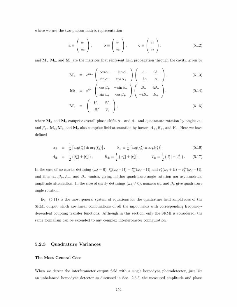
where we use the two-photon matrix representation

a ≡

a1

a2

, b ≡

b1

b2

, c ≡

c1

c2

, (5.12)

and Ma,Mb, and Mc are the matrices that represent field propagation through the cavity, given by

Ma ≡ eiα−

cosα+ − sinα+

sinα+ cosα+

A+ iA−

−iA− A+

, (5.13)

Mb ≡ eiβ−

cosβ+ − sinβ+

sinβ+ cosβ+

B+ iB−

−iB− B+

, (5.14)

Mv ≡

V+ iV−

−iV− V+

, (5.15)

where Ma and Mb comprise overall phase shifts α− and β− and quadrature rotation by angles α+

and β+. Ma,Mb, and Mv also comprise field attenuation by factors A+, B+, and V+. Here we have

defined

α± ≡ 1

2

[

arg(tsa) ± arg(tia)]

, β± ≡ 1

2

[

arg(rsb) ± arg(ri

b)]

, (5.16)

A± ≡ 1

2

(

|tsa| ± |tia|)

, B± ≡ 1

2

(

|rsb | ± |ri

b|)

, V± ≡ 1

2

(

|lsv| ± |liv|)

. (5.17)

In the case of no carrier detuning (ωd = 0), tsa(ωd + Ω) = ti∗a (ωd −Ω) and rsb(ωd + Ω) = ri∗

b (ωd −Ω),

and thus α+,β+, A−, and B− vanish, giving neither quadrature angle rotation nor asymmetrical

amplitude attenuation. In the case of cavity detunings (ωd 0= 0), nonzero α+ and β+ give quadrature

angle rotation.

Eq. (5.11) is the most general system of equations for the quadrature field amplitudes of the

SRMI output which are linear combinations of all the input fields with corresponding frequency-

dependent coupling transfer functions. Although in this section, only the SRMI is considered, the

same formalism can be extended to any complex interferometer configuration.

5.2.3 Quadrature Variances

The Most General Case

When we detect the interferometer output field with a single homodyne photodetector, just like

an unbalanced homodyne detector as discussed in Sec. 2.6.3, the measured amplitude and phase

154

105 106 107 108−0.4

−0.2

0

0.2

0.4

0.6

0.8

1

Frequency (Hz)

Qua

drat

ure

Rota

tion

(π)

α+(0×HWHM), β+(0×HWHM)

β+(0.3×HWHM)

β+(0.6×HWHM)

β+(0.9×HWHM)β+(1.2×HWHM)

α+(0.3×HWHM)α+(0.6×HWHM)α+(0.9×HWHM)

α+(1.2×HWHM)

Figure 5-4: Quadrature rotation angles α+ and β+ for various SRC detunings. The HWHM is thehalf linewidth at the half maximum of the SRC.

quadrature variances of the field, given by

Vc1(Ω) =⟨

|c1(Ω) − 〈c1〉|2⟩

, (5.18)

Vc2(Ω) =⟨

|c2(Ω) − 〈c2〉|2⟩

, (5.19)

(similarly for Va1 , Va2 , Vb1 , and Vb2), are found in terms of the amplitude and phase quadrature

variances of the input fields a, b, and v to be

Vc1

Vc2

=

cos2 α+ sin2 α+

sin2 α+ cos2 α+

A2+ A2

−

A2− A2

+

Va1

Va2

+

cos2 β+ sin2 β+

sin2 β+ cos2 β+

B2+ B2

−

B2− B2

+

Vb1

Vb2

+

V 2+ V 2

−

V 2− V 2

+

Vv1

Vv2

. (5.20)

This is the most general system of equations for the SRMI output quadrature variances which

are linear combinations of the quadrature variances of the input fields with frequency-dependent

coupling transfer functions. When all the fields a, b, and v are shot-noise-limited, Va1 = Va2 = Vb1 =

Vb2 = Vv2 = Vv2 = 1, and thus, Vc2 = Vc2 = 1 as expected. Although it is previously said that a, b,

155

and c are an unsqueezed field, a squeezed field, and a vacuum field, respectively, the derived model

is general enough to allow any of them to be squeezed fields or noisy fields as one wishes.

If a is shot-noise-limited at all frequencies and v is a vacuum field, not a squeezed vacuum field

to compensate for the decoherence or loss of squeezing, Va1 = Va2 = Vv1 = Vv2 = 1. Moreover, if b is

a squeezed vacuum field with a squeeze factor of r in the amplitude quadrature, Eq. (5.20) becomes

Vc1

Vc2

=

cos2 α+ sin2 α+

sin2 α+ cos2 α+

A2+ A2

−

A2− A2

+

1

1

+

cos2 β+ sin2 β+

sin2 β+ cos2 β+

B2+ B2

−

B2− B2

+

e−2r

e2r

+

V 2+ V 2

−

V 2− V 2

+

1

1

. (5.21)

The result of the squeezed quadrature variance for rs =√

0.93, rl =√

0.9995, retm =√

0.995, r =

1, wd/(2π) = 50 kHz, φd = π + π/30, and LSRC = 2 m is plotted in Fig. 5-5.

103 104 105 106 107−10

−9

−8

−7

−6

−5

−4

−3

−2

−1

0

Frequency (Hz)

Qua

drat

ure

Varia

nce

Rela

tive

to S

hot N

oise

(dB)

DetunedResonant

Figure 5-5: The simulation results of the squeezed quadrature variance of an interferometer outputfield for rs =

√0.93, rl =

√0.9995, retm =

√0.995, r = 2,φd = π + π/30, and L = 2 m in two cases:

(a) wd/(2π) = 10 kHz and (b) wd/(2π) = 0. The squeezing level decrease at frequencies below 1MHz is due to the cavity pole of the SRC.

156

Case of No Cavity Detuning

In the case of no cavity detuning (ωd = 0), α+ = β+ = 0 and A− = B− = V− = 0, and therefore,

there is no cross-coupling between the amplitude and phase quadrature variances of the interferom-

eter input and squeezed vacuum fields. This simplifies Eq. (5.20) to be

Vc1

Vc2

= A2+

Va1

Va2

+ B2+

Vb1

Vb2

+ V 2+

Vv1

Vv2

, (5.22)

where A+, B+, and V+ are also simplified to be

A+ = |tsa| =tmts

√

1 + r2mr2

sr2l − 2rmrsrl cos(2ΩLSRC/c)

, (5.23)

B+ = |rsb | =

√

r2s + (r2

s + t2s)2r2

l r2m − 2(r2

s + t2s)rsrlrm cos(2ΩLSRC/c)

1 + r2mr2

sr2l − 2rmrsrl cos(2ΩLSRC/c)

, (5.24)

V+ = |lsv| =√

1 − |tsa|2 − |rsb |2. (5.25)

Again, if a is shot-noise-limited at all frequencies and v is a vacuum field, Va1 = Va2 = Vv1 =

Vv2 = 1. In addition, if b is a squeezed vacuum field with a squeeze factor of r in the amplitude

quadrature, Eq. (5.22) becomes

Vc1

Vc2

=(

1 − |rsb |2

)

1

1

+ |rsb |2

e−2r

e2r

. (5.26)

A result of the squeezed quadrature variance for rs =√

0.93, rl =√

0.9995, retm =√

0.995, r =

1, wd/(2π) = 0 Hz, φd = π + π/30, and LSRC = 2 m is also plotted in Fig. 5-5.

5.3 Theory of Quantum-Enhancement in Advanced Interfer-

ometer Configurations

Long baseline laser-interferometric GW detectors such as LIGO, VIRGO, GEO600, and TAMA300

are based on a Michelson interferometer with a Fabry-Perot cavity in each arm and a power-recycling

cavity (PRC) formed from a mirror called a power-recycling mirror (PRM) between the laser source

and the Michelson interferometer to increase the optical gain of the displacement measurement

or equivalently increase the signal-to-shot-noise ratio. The next generation GW detectors such as

Advanced LIGO are planned to improve their sensitivities by making use of even higher laser powers

[95, 7].

The next generation GW detectors also plan to employ a detuned SRM in order to manipulate

and optimize the frequency response of the detectors to possible GW signals. The SRC is detuned

157

from carrier resonance to recycle a GW signal at some frequencies and resonantly extract it at

other frequencies [208, 209]. This configuration is called the resonant sideband extraction (RSE). A

detuned SRC exhibits two optical resonances at frequencies in the GW detection band that can be

chosen to optimize the sensitivity in the presence of other noise sources, as shown in Fig. 1-8. The

peak at a higher frequency arises from the unbalanced response of a GW sideband resonating in

the detuned SRC. The peak at a lower frequency arises because the GW sidebands induced by the

differential displacement of the arms enter the detuned SRC, forming a radiation pressure induced

opto-mechanical spring which enhances the optical response at the resonant frequency of the spring

[96, 101]. The configuration allows the possibility of overcoming the standard quantum limit (SQL),

which has been addressed in Sec. 1.4.3.

As discussed in Sec. 1-8, a Michelson interferometer with Fabry-Perot cavity arms is optically

equivalent to a simple Michelson interferometer with arms that possess cavity frequency responses.

Likewise, a Michelson interferometer with two Fabry-Perot cavity arms and both a PRC and SRC is

optically equivalent to a three-mirror cavity that consists of the PRM, Michelson-equivalent mirror,

and SRM [210]. However, the two-photon transfer function of such an interferometer with unequal

losses and reflectivities in the arms is extremely complex, and therefore the propagation of a squeezed

vacuum field in the interferometer and its interaction with the interferometer field are better under-

stood by use of computer simulations. A few computer programs are available to calculate signal

and noise fields in complex interferometers [103]. Fig. 1-8 shows the result of a computer simulation

of quantum-enhancement in Advanced LIGO.

158

Chapter 6

Demonstration of Quantum

Enhancement in a Gravitational

Wave Detector

6.1 Overview

In the previous chapters, the techniques necessary for the implementation of quantum-enhancement

in long baseline laser-interferometric gravitational wave (GW) detectors have been studied. The

generation, degradation, detection, and control of squeezed states using a sub-threshold optical

parametric oscillator (OPO) and a homodyne detector have been theoretically discussed in Chap. 2

and experimentally demonstrated in Chap. 3. The key requirements for the implementation of the

quantum-enhancement in GW detectors such as squeezing in the GW detection band, the high level

of squeezing, the long-term stability of squeezing, and frequency-dependent squeezing have been

investigated in Chap. 4. The propagation of a squeezed vacuum field in a GW detector, especially

in a signal-recycled Michelson interferometer (SRMI) configuration, and its interaction with the

interferometer field have been theoretically formulated in Chap. 5. With these building blocks, an

experimental test of quantum-enhancement in a GW detector is ready to be conducted.

In this chapter, the apparatus and results of the quantum-enhancement experiment in the LIGO

40m prototype interferometer at California Institute of Technology (Caltech) [15] are presented.

In Sec. 6.2, the role of the Caltech 40m LIGO interferometer prototype is described. In Sec.

6.3, the details of the squeezer, the prototype interferometer, the interface of the squeezer to the

interferometer, the length sensing photodetector, and the readout and control schemes are presented.

In Sec. 6.4, the experimental results of broadband quantum-enhancement and an increase in signal-

159

to-noise ratio (SNR) by squeezing are described.

6.2 Caltech 40m LIGO Interferometer Prototype

The Caltech 40m LIGO Prototype Interferometer plays an important role in Advanced LIGO R&D

as a test bed or staging area for the design, testing, refinement, and staging of advanced GW detector

configurations anticipated for Advanced LIGO, which require a full interferometer for testing. It is

anticipated that Advanced LIGO will operate with both power- and signal-recycling mirrors (PRM

and SRM), operated in the resonant sideband extraction (RSE) configuration. These signal recycling

techniques need to be prototyped with a full interferometer.

The interferometer can also be used as a test bed or staging area for the design, testing, re-

finement, and staging of other advanced detector elements. With its full control systems similar to

Advanced LIGO’s, the Caltech 40m LIGO Interferometer Prototype is an ideal choice for testing

quantum-enhancement before implementing it in long baseline GW detectors such as LIGO. The

details of the conceptual design of the Caltech 40m LIGO Interferometer Prototype can be found

in Ref. [165]. Although quantum-enhancement is compatible with an output mode cleaner (OMC)

that is planned to be used in Advanced LIGO, the experiment is conducted without an OMC since

it is not ready at the time of the experiment.

6.3 Experimental Apparatus

6.3.1 Overview

As shown in Fig. 6-1, the quantum-enhanced prototype GW detector consists of the following

components: (1) a pre-stabilized laser (PSL) system that is the light source of the interferometer

and squeezed vacuum generator that includes a Nd:YAG Master Oscillator Power Amplifier (MOPA)

laser with a throughput of 5 W at 1064 nm and all the optical and electro-optical devices to stabilize

the frequency, amplitude, and mode of the laser, (2) a triangular optical cavity – or mode cleaner –

which consists of three free hanging mirrors with a linewidth of 4 kHz, (3) a test interferometer in

a signal-recycled Michelson interferometer configuration that comprises a 50/50 beamsplitter, two

high-reflective end mirrors, and a SRM, all suspended as single loop pendulums, (4) a squeezed

vacuum generator – or squeezer – that consists of a second-harmonic generator (SHG), an optical

parametric oscillator (OPO), a monitor homodyne detector, subcarrier optics to lock the OPO cavity,

and an optical circulator to inject the generated squeezed vacuum field to the antisymmetric port

of the interferometer, and (5) a length sensing detector that consists of a high quantum efficiency

photodetector to sense differential motion of the interferometer mirrors. In the following sections,

the details of each major component are described.

160

PO

λ/4

Nd:YAGMOPA LASER

AuxiliaryNd:YAG LASER

BS

FICPO

FI

FI

BS

BS

PO BS BS PO

PO

PBS

PBS

PBS

PBS

DBS

DBS

PM5

PM4

PM3

PM2

PM1

PM6

AOMλ/4

FI

FOC

PZT3

PZT5

PZT4

PZT6

PZT1PZT2

ReferenceCavity

FR

FM

BS

PD8

PD4

PD3

PD2

PD5

PD6

PD10

PD11HPD1

HPD2

PD9

PD1

TestMass

TestMass

BS

λ/2

λ/2

λ/2

λ/2

OPO

SHG

InterferometerModeCleaner

Squeezer

SignalRecycling

Mirror

LengthSensingDetector

PO

PD7

Pre-StabilizedLaser

PMC

Figure 6-1: A schematic of the quantum-enhanced prototype gravitational wave detector that con-sists of the following parts: (1) a pre-stabilized laser (PSL) system that is the light source of theinterferometer and squeezed vacuum generator that includes a Nd:YAG Master Oscillator PowerAmplifier (MOPA) laser with a throughput of 5 W at 1064 nm and all the optical and electro-optical devices to stabilize the frequency, amplitude, and mode of the laser, (2) a triangular opticalcavity – or mode cleaner (MC) – which consists of three free hanging mirrors with a linewidth of4 kHz, (3) a test interferometer in a SRMI configuration that comprises a 50/50 beamsplitter, twohigh-reflective end mirrors, and a SRM, all suspended as single loop pendulums, (4) a squeezedvacuum generator – or squeezer – that consists of a second-harmonic generator (SHG), an opti-cal parametric oscillator (OPO), a monitor homodyne detector, subcarrier optics to lock the OPOcavity, and an optical circulator to inject the generated squeezed vacuum field to the antisymmet-ric port of the interferometer, and (5) a length sensing detector that consists of a high quantumefficiency photodetector to sense differential motion of the interferometer mirrors. BS: 50/50 beam-splitter, DBS: dichroic beamsplitter, PD1-PD11: photodetectors, HPD1 and HPD2: homodynephotodetectors, PO: pickoff mirror, λ/2: half-wave plate, λ/4: quarter-wave plate, PBS: polarizingbeamsplitter, PMC: pre-mode cleaner, AOM: acousto-optic modulator, PM1-6: electro-optic mod-ulators as phase modulators, PZT1-6: piezo-electric transducers, FI: Faraday isolator, FR: Faradayrotator, FIC: fiber input coupler, FOC: fiber output coupler, FM: flipper mirror. The referencecavity, pre-mode cleaner, mode cleaner, signal-recycling cavity, SHG, and OPO are controlled usingthe Pound-Drever-Hall locking technique.

161

6.3.2 Pre-Stabilized Laser

The PSL system is the light source of the interferometer and squeezed vacuum generator that includes

a Lightwave MOPA laser (Lightwave Electronics Inc.) with a throughput of 5 W at 1064 nm and all

the optical and electro-optical devices to stabilize the frequency, amplitude, and mode of the laser

[166]. It was designed and developed by Lightwave Electronics Inc. in collaboration with the LIGO

group. The MOPA laser is based on a diode-pumped, narrow-linewidth, single-frequency laser as the

master oscillator and a double-passed power amplifier. The PSL consists of three major components:

the frequency stabilization servo system (FSS), the intensity servo system (ISS), and the pre-mode

cleaner (PMC). The laser has three frequency actuators: a PZT of the master oscillator (fast), an

electro-optic modulator (medium), and a Peltier element that controls the temperature of the master

oscillator (slow). The electro-optic modulator (EOM) can also be used as an amplitude stabilization

actuator.

In the FSS, the laser is frequency-locked to one of the resonance frequencies of a monolithic

optical cavity suspended in a vacuum chamber as a frequency reference, using the Pound-Drever-

Hall (PDH) locking technique. An error signal for controlling the laser frequency is fed back to

the frequency actuators. In this way the frequency noise is reduced by the FSS and limited by the

stability of the reference cavity. To match the frequency of the laser with the resonance frequency

of the cavity, an acousto-optic modulator (AOM) shifts the laser frequency by 3.3 MHz and allows

additional servos (mode cleaner and the arm common mode) to further change the laser frequency,

while keeping the laser resonant in the reference cavity. The length, free spectral range (FSR),

finesse, and FWHM bandwidth of the reference cavity are 203.3 mm, 736.5 MHz, 9518, and 77.4

kHz, respectively. The EOM modulation frequency for the PDH technique is 21.5 MHz [211].

In the ISS, a small portion of the laser is measured by a photodetector after the PMC and the

signal is sent to feedback control electronics, yielding an error signal [212]. It is fed back to the

diode current actuator and EOM. A relative intensity noise of 10−8 Hz−1/2 between 100 Hz and 1

kHz and 5 × 10−6 Hz−1/2 between 1 kHz and 100 kHz is achieved.

The PMC is a triangular cavity that filters out higher-order Gaussian modes of the input beam.

The laser after the PMC is mainly a Gaussian TEM00 mode, and this helps decrease the intensity

noise of the laser. The PDH technique is used to generate an error signal, which is fed back to the

PZT on the concave mirror located at the edge of the PMC. The length, FSR, finesse (high), and

FWHM bandwidth (high) of the PMC are 210 mm, 713.8 MHz, 4100, and 174 kHz, respectively.

The EOM modulation frequency for the PDH technique is 35.5 MHz [211].

162

6.3.3 Mode Cleaner

Before the PSL-enhanced laser is injected into the interferometer, the triangular optical cavity or

the MC with a linewidth of 4 kHz serves to further suppress the laser intensity and frequency

fluctuations, and to filter out higher-order spatial modes of the input beam. It also plays a role

in giving a low beam position and pointing jitter. The MC consists of three free hanging mirrors

with a half-length of 13.5 m. The length is carefully chosen such that two sets of RF sidebands (33

MHz and 166 MHz) that are used to lock the Michelson interferometer and signal-recycling cavity

(SRC) respectively can transmit through the MC. The suspended optics are placed on passive seismic

isolation stacks within a single vacuum volume with a pressure of 10−6 torr. The MC is locked to

the laser using the PDH technique.

6.3.4 Interferometer

Components

The interferometer consists of three free hanging mirrors and a balanced beamsplitter, all suspended

as single loop pendulums that attenuate seismic noise at frequencies above the pendulum resonant

frequency (∼ 1 Hz), and therefore, the optics behave as free masses above the pendulum resonant

frequency. A feedback control system suppresses the seismically driven motion of the suspended

mirrors. Four pairs of magnets affixed to each optic, along with current-carrying coils, act as

actuators to keep the SRC locked on resonance to the laser frequency. The SRM and Michelson

interferometer form the SRC to enhance the detector sensitivity. The suspended optics are placed on

passive vibration isolation stacks within the single vacuum volume with the same pressure of 10−6

torr as the MC. More details about the interferometer components can be found in Refs. [95, 165].

Configuration

The SRMI configuration is chosen since it is an important feature of the optical configuration en-

visioned for Advanced LIGO [7, 95]. The Michelson interferometer is locked on a dark fringe with

a small offset such that a small amount of the carrier light comes out of the SRC, while the SRC

is locked on resonance to the carrier. The carrier light at the antisymmetric port acts as a local

oscillator field (LO) that a GW-induced signal beats against – this is called the DC readout scheme

[7].

Two sets of RF sidebands at 33 MHz and 166 MHz are generated by the phase modulators, PM3

and PM4, respectively. The photodetector at the symmetric port (PD6) is used to lock the SRC and

the photodetector in one of the Michelson arms (PD7) is used to lock the Michelson interferometer.

Once the Michelson offset is introduced, the photodetector used for locking the offseted Michelson is

switched from the PD7 to the length sensing photodetector (PD11) for stabilizing the optical power

163

at the PD11. The Michelson interferometer and SRC locking schemes will be described in Sec. 6.3.7.

Displacement Sensitivity

The displacement sensitivity of the interferometer is shown in Fig. 6-5. The comparison between the

measured sensitivity without squeezing and the theoretically predicted shot-noise-limited displace-

ment sensitivity based on the measured optical power of 100 µW indicates that the interferometer is

shot-noise-limited at frequencies above 42 kHz. At frequencies below 42 kHz, the noise is dominated

by laser intensity noise and interferometer length noise that appear in the differential motion of the

arms. The peaks at frequencies above 42kHz are also due to the interferometer length noise. In

addition, the optical power at the antisymmetric port is changed to verify the√

P scaling of the

shot noise as shown in Fig. 6-2. The figure shows that as the optical power doubles, the noise floor

increases by 3 dB at frequencies above 42 kHz and by 6 dB at frequencies below 42 kHz, indicating

that the detector is shot-noise-limited above 42 kHz. Below 42 kHz, the detector is dominated by

the laser noise. Quantum radiation pressure noise is buried under the laser noise as well as other

technical noise, and only the shot noise is accessible for showing quantum-enhancement1.

104 105−165

−160

−155

−150

−145

−140

−135

−130

−125

−120

Frequency [Hz]

Noise

Lev

el [1

0log

(Vrm

s2

/Hz)

]

50 µW

100 µW

200 µW

Photodetector Dark Noise

Figure 6-2: The noise floor of the SRMI detector for different optical powers at the length sensingphotodetector. As the optical power doubles, the noise floor increases by 3 dB at frequencies above42 kHz and by 6 dB at frequencies below 42 kHz, indicating that the detector is shot-noise-limitedabove 42 kHz. Below 42 kHz, the detector is dominated by the laser noise. For the proper comparisonof the noise floors at different powers, the photodetector noise must be subtracted from each noisefloor.

1As of today, no interferometer has ever seen quantum radiation pressure noise, not just the experiments withinjected squeezing.

164

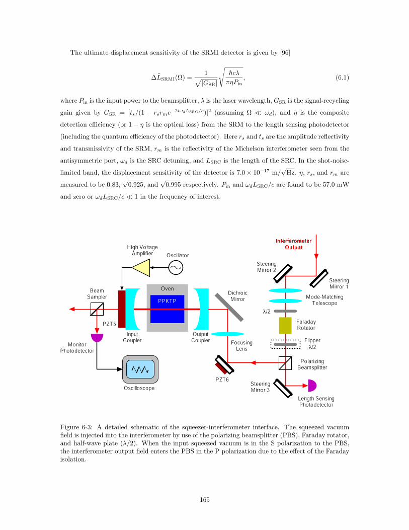
The ultimate displacement sensitivity of the SRMI detector is given by [96]

∆LSRMI(Ω) =1

√

|GSR|

√

hcλ

πηPin, (6.1)

where Pin is the input power to the beamsplitter, λ is the laser wavelength, GSR is the signal-recycling

gain given by GSR = [ts/(1 − rsrme−2iωdLSRC/c)]2 (assuming Ω + ωd), and η is the composite

detection efficiency (or 1 − η is the optical loss) from the SRM to the length sensing photodetector

(including the quantum efficiency of the photodetector). Here rs and ts are the amplitude reflectivity

and transmissivity of the SRM, rm is the reflectivity of the Michelson interferometer seen from the

antisymmetric port, ωd is the SRC detuning, and LSRC is the length of the SRC. In the shot-noise-

limited band, the displacement sensitivity of the detector is 7.0 × 10−17 m/√

Hz. η, rs, and rm are

measured to be 0.83,√

0.925, and√

0.995 respectively. Pin and ωdLSRC/c are found to be 57.0 mW

and zero or ωdLSRC/c + 1 in the frequency of interest.

DichroicMirror

OutputCoupler

PZT5

PPKTP

MonitorPhotodetector

Oven

High VoltageAmplifier Oscillator

InputCoupler Focusing

Lens

Mode-MatchingTelescope

SteeringMirror 2

SteeringMirror 1

FaradayRotator

BeamSampler

λ/2

Flipperλ/2

SteeringMirror 3

Length SensingPhotodetector

PolarizingBeamsplitter

Oscilloscope

PZT6

Figure 6-3: A detailed schematic of the squeezer-interferometer interface. The squeezed vacuumfield is injected into the interferometer by use of the polarizing beamsplitter (PBS), Faraday rotator,and half-wave plate (λ/2). When the input squeezed vacuum is in the S polarization to the PBS,the interferometer output field enters the PBS in the P polarization due to the effect of the Faradayisolation.

165

6.3.5 Squeezed Vacuum Generator

Overview

The squeezed vacuum generator or squeezer is essentially identical to the squeezer discussed in Chap.

3 except for the photodetector. The squeezer consists of a SHG, an OPO, a monitor homodyne

detector, subcarrier optics to lock the OPO cavity, and an optical circulator to inject the generated

squeezed vacuum field to the antisymmetric port of the interferometer. The squeezer is powered by

1.5 W of the Nd:YAG MOPA laser that also powers the SRMI detector. In this section, the squeezed

vacuum injection optics are mainly described while the SHG, OPO, subcarrier optics, and monitor

homodyne detector have been described in Chap. 3.

SHG, OPO, and Subcarrier Optics

The SHG, OPO, and subcarrier optics are essentially identical to the squeezer components in Chap.

3, and therefore, they will not be discussed here. For details, Chap. 3 should be reviewed.

Monitor Homodyne Detector

A balanced homodyne detector is used to monitor the generated squeezed vacuum field before

injecting it to the interferometer. The monitor homodyne detector is essentially identical to the

homodyne detector discussed in Chap. 3, and therefore, it will not be discussed here. For details,

Chap. 3 should be reviewed.

As shown in Fig. 6-1, a flipper mirror is installed in the path of the squeezed vacuum field. When

the flipper mirror is up, the squeezed vacuum is directed toward the monitor homodyne detector to

monitor the level of squeezing before the injection. When the flipper mirror is down, the squeezed

vacuum is injected into the interferometer.

Squeezed Vacuum Injection Optics

A detailed schematic of the interface of the squeezer to the interferometer is shown in Fig. 6-3.

The squeezed vacuum field is injected into the interferometer via a polarizing beamsplitter (PBS),

Faraday rotator, and half-wave plate. When the input squeezed vacuum is in the S polarization to

the PBS, the squeezing-enhanced interferometer output field enters the other port of the PBS in the

P polarization due to the effect of the Faraday isolation.

Another important set of optical components is steering mirrors and mode-matching optics.

However, to align and mode-match the input squeezed vacuum field to the interferometer mode

is not an easy task since the squeezed vacuum field and interferometer output field are counter-

propagating. This is done by optimizing the transmission of the interferometer output field through

166

the OPO cavity in a TEM00 mode using the steering mirrors and mode-matching telescope. The

alignment and mode-matching procedure is as follows:

1. Block the seed and subcarrier and scan the OPO cavity using the PZT on the input cou-

pler (PZT5). Set up a photodetector in the seed path to monitor the transmission of the

interferometer field through the OPO cavity.

2. Flip the flipper half-wave plate in between the Faraday rotator and PBS. The orientation of

the half-wave plate is such that the interferometer field is directed toward the OPO cavity.

When the flipper is not in place, the orientation of the half-wave plate between the Faraday

rotator and mode-matching telescope is such that the field transmits through the PBS toward

the length sensing photodetector.

3. Align and mode-match the interferometer output field through the OPO cavity using steering

mirrors 1 and 2 and the mode-matching telescope. When the OPO cavity is scanned, the mode

structure measured by the monitor photodetector indicates the coupling of the interferometer

mode to the OPO cavity mode or equivalently the optical loss due to the mode-mismatch

between the interferometer and squeezed vacuum field. Once it is optimized, the procedure

ensures the squeezed vacuum field to be aligned and mode-matched to the interferometer.

4. Now that the squeezed vacuum injection path has been optimized, the interferometer field path

has also been determined. Use steering mirror 3 to align the beam onto the length sensing

photodetector.

The squeeze angle is locked to the amplitude quadrature of the interferometer field by the noise-

locking technique using the PZT-actuated mirror (PZT6) in Fig. 6-1. The squeeze angle readout

and control scheme will be described in Sec. 6.3.7.

6.3.6 Length Sensing Photodetector

To measure the quantum-enhancement in the differential motion in the arms of the prototype GW

detector, a high quantum efficiency photodiode in a transimpedance amplifier is used. The pho-

todiode is an ETX500T photodiode (JDS Uniphase) with a quantum efficiency of 93%. The op-

erational amplifier used for the transimpedance amplifier is OPA657 (Texas Instrument) and the

transimpedance is 10 kΩ. Its input voltage noise and input current noise are 4.8 nV/√

Hz and 1.3

fA/√

Hz at frequencies above 100 Hz respectively. This operational amplifier is chosen because its

low input current noise allows the photodetector to be Johnson-noise-limited in the frequency band

between 100 Hz and 10 MHz. This ensures about 8 dB of separation between the electric noise of

the photodetector and the shot noise of 100 µW. The measured noise floor of the photodetector is

167

shown in Fig. 6-2. A broadband noise floor of about 7 nV/√

Hz is achieved with this photodetector

circuit.

(a)

(c)

(e)(d)

(b)

Envelope Detector50Ω Load Impedance

RF Low-Pass Filter5MHz Cutoff50Ω System

Buffer1MΩ Load Impedance

600Ω Source Impedance

RF Amplifier20dB Gain

50Ω Load Impedance50Ω Source Impedance

Oscilloscope1MΩ Load Impedance

HP8591E Spectrum Analyzer50Ω Load Impedance

Active High-Pass Filter100Hz Cutoff

1MΩ Load Impedance600Ω Source Impedance

SR785 Spectrum Analyzer100MΩ Load Impedance

Photodetector50Ω SourceImpedance

Amplifier40dB Gain

1MΩ Load Impedance600Ω Source Impedance

InterferometerOutput Field

OpticalCirculator

PZT6

RF Power Splitter50Ω System

Low-Pass Filter1kHz Cutoff

RF Band-Pass Filter2MHz-100MHz

Frequency Band

MichelsonOffset

OffsetInput

Oscillator

Mixer

Adder


Low-Pass Filter1kHz Cutoff

Variable GainAmplifier

Figure 6-4: A detailed schematic of the readout and control schemes to (a) detect the squeezing-enhanced interferometer output field, (b) control the Michelson offset, (c) monitor the level ofsqueezing, (d) control the squeeze angle using the noise-locking technique and the PZT-actuatedmirror (PZT6), and (e) measure the broadband quantum-enhancement.

6.3.7 Readout and Control Schemes

The readout and control schemes to (a) detect the squeezing-enhanced interferometer output field,

(b) control the Michelson offset, (c) monitor the level of squeezing, (d) control the squeeze angle

using the noise-locking technique, and (e) measure the broadband quantum-enhancement are shown

in Fig. 6-4. The length sensing photodetector measures the squeezing-enhanced interferometer

output field. The output of the photodetector is low-pass filtered with a cutoff frequency of 5 MHz

to remove the beats between the carrier and 33 MHz sidebands and between the carrier and the 166

MHz sidebands. The output of the low-pass filter is high-pass filtered with a cutoff frequency of

100 Hz, amplified by an amplification factor of 100, and measured by the SR785 spectrum analyzer

(Stanford Research Systems) to see the noise spectrum of the interferometer. The 5 MHz low-pass

filter output is also measured via the RF amplifier by the HP8591E spectrum analyzer (Hewlett-

Packard) to monitor the level of squeezing at MHz frequencies. The output of the RF amplifier is

also used to lock the squeeze angle using the quantum noise locking technique. The phase modulator

168

used in this experiment is the PZT (PZT6) in Fig. 6-1. The output of the 5 MHz low-pass filter is

also measured by the oscilloscope to monitor the DC power fluctuations of the interferometer output

field. It is also compared with a Michelson offset setting value by the differential amplifier and its

output is fed back to the coil drivers that actuate on the Michelson mirror positions.

Some preparation is required to calibrate the shot noise and observe quantum-enhancement in the

interferometer. The procedure for controlling the Michelson offset and squeeze angle and measuring

the effect of the broadband quantum-enhancement in the interferometer is the following:

1. Block the squeezed vacuum not to inject it into the interferometer, or equivalently let random

vacuum noise enter the interferometer. This is necessary to calibrate the shot noise level in

the interferometer before observing the effect of squeezing.

2. Lock the interferometer using the PD6, PD7, and RFPD which is located at the interferometer

output port between the optical circulator and PD11 via a flipper mirror (not shown in the

figure). Also, make sure that the carrier-to-sideband power ratio is sufficiently high so that

the contribution of the sideband shot noise to the overall shot noise level is small2. This can

be verified by using an optical spectrum analyzer (scanning Fabry-Perot cavity).

3. Flip down the flipper mirror after switching to the PD6 and PD7 from the RFPD (so that the

interferometer lock does not drop) and detect the interferometer output field with the PD11.

Filter out the 33 MHz and 166 MHz beats with the carrier. Make sure on the oscilloscope that

the DC power level is constant.

4. Turn on the Michelson offset feedback control system and set the offset to an optimum value

so that the power of the interferometer output field at the PD11 is 100 µW. Increase the

control gain to stabilize the shot noise so that its fluctuation level is within the possible level

of squeezing.

5. Measure the broadband noise power of the interferometer field with the SR785 spectrum ana-

lyzer. Make sure that the shot noise level is sufficiently higher than the electronic noise of the

measurement system. Compare the measured shot noise level with the theoretically predicted

shot noise level.

6. Change the laser power at the PD11 to see how the noise power changes with the increasing

or decreasing laser power. If it is shot noise, it goes up by 3 dB as the laser power doubles. If

it is laser intensity or frequency noise, it goes up by 6 dB as it doubles. This gives an estimate

of the cutoff frequency of squeezing.

2Another way of minimizing the effect of the sidebands is to place an OMC between the output port of the inter-ferometer beamsplitter and the photodetector and reject the sidebands outside the linewidth of the OMC. However,this might degrade the level of squeezing by introducing an extra optical loss due to the possible mode-mismatchbetween the OMC and the squeezed vacuum field.

169

7. Inject the squeezed vacuum into the interferometer. Start with a low squeezing level (by

attenuating the OPO pump power) not to disturb the lock of the interferometer (although, in

principle, it should not disturb it). Make sure that the optical crosstalk between the OPO and

interferometer is sufficiently attenuated by tweaking the Faraday isolator.

8. Scan the squeeze angle using the PZT6 to verify the effect of squeezing with the HP8591E

spectrum analyzer. This gives an estimate of how much the injection of squeezing reduces the

shot noise.

9. Turn on the noise-locking feedback control system to lock the squeeze angle to the squeezed

quadrature. Optimize the control gain and phase and modulation frequency.

10. Measure the broadband noise power of the interferometer with the SR785 spectrum analyzer

to verify the broadband quantum-enhancement. Monitor the HP8591E spectrum analyzer and

the oscilloscope to check if the interferometer stays locked during the measurement.

11. Excite the interferometer beamsplitter to simulate a GW signal at a frequency where the shot

noise is flat and verify an increase in SNR by the injection of the squeezed vacuum. If the

effect of squeezing is proper, the simulated GW signal strength does not change regardless of

the presence of squeezing.

6.4 Experimental Results

6.4.1 Overview

With all the necessary components ready, the squeezing injection has been tested. In the following

sections, experimental results of broadband squeezing-enhancement in the prototype GW detector

in the quantum noise limited frequency band and an increase in SNR with a simulated GW signal

by the squeezing-enhancement are presented.

6.4.2 Broadband Squeezing-Enhancement in the Interferometer

The effect of quantum-enhancement in the SRMI detector is represented by squeeze factor r in the

displacement sensitivity of the detector in Eq. 6.1 such that

∆LSRMI(Ω) =1

√

|GSR|

√

hcλ

πηPine−r (6.2)

or in terms of the familiar quadrature variance,√

V (Ω) = e−r. This is an approximate form of the

most rigorous equation given in Refs. [96, 82]. The squeeze factor r is a function of η, rm, rs, and ωd

as discussed in Sec. 5.2. Since the frequency of interest Ω is much smaller than the linewidth of the

170

104 10510−17

10−16

10−15

Frequency [Hz]

Disp

lace

men

t [m

/Hz1/

2 ]

Squeezed Shot NoiseTheoretically Predicted Shot Noise

Shot Noise

Figure 6-5: The noise floor of the SRMI detector with and without the injection of a squeezed vacuumfield. The theoretically predicted shot noise level based on the measured optical power is comparedwith the measured noise floor of the SRMI detector. The interferometer is shot-noise-limited atfrequencies above 42 kHz. With the squeezing injection, the shot noise is reduced broadband inthe shot-noise-limited frequency band by a squeeze factor of r = 0.34. The peak at 18 kHz in thesqueezing spectrum is due to the PZT modulation for the noise locking technique. The other peaksare due to the interferometer input PZT noise coupled to the interferometer length noise.

SRC, Eq. (6.2) can be approximated as a frequency-independent equation. When the displacement

sensitivity is normalized to the shot noise level to see the effect of squeezing, Eq. (6.2) can be divided

by Eq. (6.1) to obtain

∆LSRMI

∣

∣

∣

Squeezed

∆LSRMI

∣

∣

∣

Unsqueezed

= e−r. (6.3)

The result of the broadband squeezing-enhancement in the interferometer is shown in Fig. 6-5.

The comparison between the two spectra shows that the quantum noise floor of the interferometer

is reduced by the injection of the squeezed vacuum field by a squeeze factor of r = 0.34 in the shot-

noise-limited frequency band. This is equivalent to a factor of 2 increase in laser power (without

squeezing) or equivalently a factor of 2 decrease in laser power for the same shot noise level when the

interferometer is squeezed. The injected squeezing level is 9.3 dB (inferred based on the measured

level of squeezing and optical losses) or 7.4± 0.1 dB (measured by the monitor homodyne detector).

The measurable squeezing effect is limited to frequencies above 42 kHz in this experiment since the

quantum noise is masked by the classical noise at lower frequencies. However, squeezing-enhancement

171

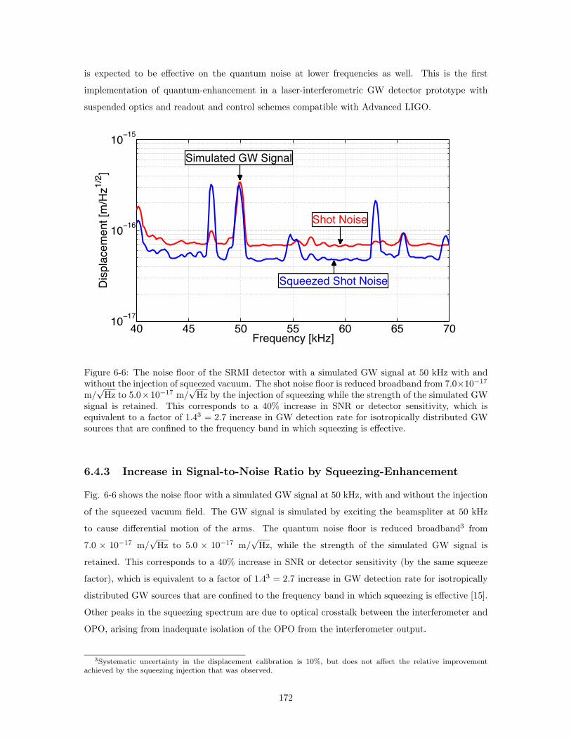
is expected to be effective on the quantum noise at lower frequencies as well. This is the first

implementation of quantum-enhancement in a laser-interferometric GW detector prototype with

suspended optics and readout and control schemes compatible with Advanced LIGO.

40 45 50 55 60 65 7010−17

10−16

10−15

Frequency [kHz]

Disp

lace

men

t [m

/Hz1/

2 ]

Simulated GW Signal

Shot Noise

Squeezed Shot Noise

Figure 6-6: The noise floor of the SRMI detector with a simulated GW signal at 50 kHz with andwithout the injection of squeezed vacuum. The shot noise floor is reduced broadband from 7.0×10−17

m/√

Hz to 5.0×10−17 m/√

Hz by the injection of squeezing while the strength of the simulated GWsignal is retained. This corresponds to a 40% increase in SNR or detector sensitivity, which isequivalent to a factor of 1.43 = 2.7 increase in GW detection rate for isotropically distributed GWsources that are confined to the frequency band in which squeezing is effective.

6.4.3 Increase in Signal-to-Noise Ratio by Squeezing-Enhancement

Fig. 6-6 shows the noise floor with a simulated GW signal at 50 kHz, with and without the injection

of the squeezed vacuum field. The GW signal is simulated by exciting the beamspliter at 50 kHz

to cause differential motion of the arms. The quantum noise floor is reduced broadband3 from

7.0 × 10−17 m/√

Hz to 5.0 × 10−17 m/√

Hz, while the strength of the simulated GW signal is

retained. This corresponds to a 40% increase in SNR or detector sensitivity (by the same squeeze

factor), which is equivalent to a factor of 1.43 = 2.7 increase in GW detection rate for isotropically

distributed GW sources that are confined to the frequency band in which squeezing is effective [15].

Other peaks in the squeezing spectrum are due to optical crosstalk between the interferometer and

OPO, arising from inadequate isolation of the OPO from the interferometer output.

3Systematic uncertainty in the displacement calibration is 10%, but does not affect the relative improvementachieved by the squeezing injection that was observed.

172

Chapter 7

The Future

7.1 Overview

In Chap. 6, quantum-enhancement in the Caltech 40m LIGO Interferometer Prototype using the

techniques described in Chaps. 2, 3, 4, and 5 has been experimentally demonstrated. Although the

proof-of-principle of quantum-enhanced gravitational wave (GW) detectors has been demonstrated,

several possible improvements can be incorporated into the techniques used in Chap. 6. In this

chapter, some possible future improvements and investigations are proposed and studied.

7.2 Possible Future Improvements

7.2.1 Bow-Tie Optical Parametric Oscillators

It has been shown in Sec. 4.2 that any scattered light (which is not shot noise limited) from a

homodyne detector or an interferometer couples into an optical parametric oscillator (OPO) as

a seed and degrades squeezing at low frequencies. In Advanced LIGO, the optical power of the

interferometer output field in the DC readout scheme [7, 95] is about 100 mW. Although back-

scattered light can be substantially avoided by placing a multiple number of Faraday isolators in

the squeezing injection path, this solution is not realistic since Faraday isolators are typically lossy

(about 10%) and using even a few of them leads to a significant loss in the level of squeezing.

One way to go around this problem is to use a cavity configuration that geometrically isolates

interferometer back-scattered light from the input squeezed vacuum. A good example is a bow-tie

cavity configuration as shown in Fig. 7-1. Even if back-scattered light couples into the OPO cavity, it

cannot couple out of the OPO cavity, and therefore, do not co-propagate with the squeezed vacuum

field. A bow-tie OPO has been demonstrated by Grosse et al. [115] although it has not been tested

with an interferometer yet. It is expected to improve the performance of squeezing in it, especially

173

at low frequencies.

SqueezedVacuum

VacuumSeed

NonlinearCrystal

Figure 7-1: A schematic of a bow-tie OPO cavity that geometrically isolates back-scattered lightfrom the squeezed vacuum field. Even if back-scattered couples into the OPO cavity, it cannotcouple out of the OPO cavity, and therefore, does not co-propagate with the squeezed vacuum field.

7.2.2 Doubly-Resonant Optical Parametric Oscillators

Another improvement is a doubly-resonant OPO. It has three advantages: (1) to increase the pump

power, (2) to mode-match the pump to the seed perfectly, and (3) to lock the OPO cavity with

the pump field. Since a high-power laser with a throughput of several watts at 1064 nm is costly

or unavailable in many situations such as LIGO, it is difficult to obtain about a few watts at 532

nm from a second-harmonic generator (SHG). However, the OPO cavity can be made resonant at

both 1064 nm and 532 nm so that the nonlinear interaction between the two fields can be enhanced.

The doubly-resonant cavity also makes it possible for both beams to be mode-matched perfectly,

indicating that no extra pump that does not interact with the seed resonates in the cavity. Since

nonlinear crystals are typically absorptive at 532 nm, the doubly-resonant OPO helps stabilize the

temperature of the crystal. The other advantage is that the OPO cavity can be locked by use of the

second-harmonic pump, due to which, a frequency-shifted subcarrier used to lock the OPO cavity

at 1064 nm is not necessary. A doubly-resonant OPO has also been demonstrated by Grosse et al.

[115].

7.3 Possible Future Investigations

7.3.1 Generation of Squeezed States in Optical Waveguides

In the past, various efforts have been made to obtain squeezed states without optical cavities so that

squeezing occurs broadband, not limited by the linewidth of the cavities. Shelby et al. demonstrated

the generation of 0.58 dB of squeezing from four-wave mixing in a 114 m long optical fiber which

was cooled down to 4.2 K to suppress Brillouin scattering [213]. It has also been shown recently that

174

optical confinement using waveguides helps increase the generation rate of correlated photon pairs.

Periodically poled waveguides, for example, produce large numbers of correlated photon pairs with

only a few µW of pump [214, 215, 216]. Fiorentino et al. demonstrated the generation of 2.9 × 106

correlated photon pairs/s per mW of pump from a periodically poled KTiOPO4 (PPKTP) waveguide

in a 1-nm band, which was more than 50 times higher than the bulk PPKTP crystal generation

rate [217]. If the optical loss in the PPKTP waveguide is decreased, the PPKTP waveguide may be

an interesting approach to the cavity-less generation of squeezed states since it is compact without

the need for an optical cavity. The cavity-less generation of squeezed states is strongly desired since

instability in the performance of squeezing mostly comes from cavities used in the squeezer such as

the OPO and SHG.

7.3.2 Generation of Squeezed States in Microcavities

Recently, Kerr-nonlinearity induced OPO in a toroidal microcavity that is a silica-based whispering-

gallery-type resonator [218, 219] has been shown by Kippenberg et al. [220]. The OPO threshold

was measured to be only 174 µW, which is more than two orders of magnitude lower than for optical-

fiber-based OPO. The micro-OPO showed a high conversion efficiency of 36% and a signal-to-idler

ratio of 97%. A phase-sensitive amplification process that can exclude competing Brillouin or Raman

processes with a highly idieal coupling junction can provide an excellent candidate system for the

generation of squeezed states of light in a microcavity.

7.3.3 Metamaterial-Enhanced Optical Parametric Oscillation

The optics community has been excited by recent demonstrations of negative-index metamaterials.

The unique properties of metamaterials were verified in Caloz et al. in 2001 [221]. Eleftheriades

et al. and Caloz et al. invented a method to realize left-handed metamaterials using artificial

lumped-element loaded transmission lines in microstrip technology [222]. The first superlens with a

negative refractive index provided resolution three times better than the diffraction limit and was

demonstrated at microwave frequencies by Grbic and Eleftheriades [223]. Subsequently, the first

optical superlens (an optical lens that exceeds the diffraction limit) was invented and demonstrated

in 2005 by Fang et al. [224].

Negative-index metamaterials can also be used in an OPO and SHG to enhance their efficiencies.

A theoretical model of the OPO and SHG enhanced by negative-index metamaterials was studied

by Popov and Shalaev [225, 226] and the metamaterial-enhanced SHG was demonstrated in 2006

by Klein et al. [227, 228]. OPO enables transparency, amplification, and oscillation with no cavity

in strongly absorbing negative index-metamaterials. The opposite directions of the wave vector and

the Poynting vector in such materials result in extraordinary optical properties, including backward

phase-matching and the generation of entangled pairs of left- and right-handed counter-propagating

175

photons. Metamaterial-enhanced OPO may be an interesting approach to increasing the level of

squeezing dramatically.

7.3.4 Quantum-Enhanced Laser Interferometers in Resonant Sideband

Extraction

The resonant sideband extraction (RSE) scheme is the interferometer configuration envisioned for

Advanced LIGO. However, squeezing-enhancement has not been tested with the RSE yet. Al-

though in principle, squeezing-enhancement should also be effective in the RSE configuration just

as squeezing-enhancement in the signal-recycled Michelson interferometer configuration has been

demonstrated, an interesting feature of the RSE is that the detuned signal-recycling cavity (SRC)

rotates the squeeze angle in the interferometer. Since a squeezed vacuum field from an OPO has a

constant squeeze angle, the injection of the squeezed vacuum into the antisymmetric port reduces

quantum noise at some frequencies, but increases it at other frequencies, especially near the arm

cavity resonance and optical spring frequencies. Therefore, to reduce the interferometer quantum

noise broadband, squeezing with a frequency-dependent squeeze angle is required. As discussed in

Sec. 4.5, filter cavities such as kilometer-scale or high-finesse empty cavities, squeeze amplitude

filter cavities, and cavities with electromagnetically induced transparency (EIT) media can be used

to overcome this problem. When radiation pressure noise becomes significant in the Advanced LIGO

interferometers, frequency-dependent squeezing in the GW detection band needs to be investigated

before implementing squeezing in the detectors.

7.3.5 Quantum-Enhanced Laser Interferometers with an Output Mode

Cleaner

An output mode cleaner (OMC) is planned to be installed in Advanced LIGO [7, 95]. The purpose

of the OMC is to clean the mode of the interferometer output field and to remove all RF sidebands

so that oscillator phase noise does not couple in and the perfect overlap of the LO and GW signals

at the length sensing photodetector is ensured. Therefore, the OMC will play an important role in

Advanced LIGO. However, squeezing with the OMC has not been tested yet.

Presumably there will be some mode-mismatch between the OMC and interferometer output

field, which leads to some optical loss which is expected to be about 20%, indicating that about

20% of squeezing is lost. Although this test is fairly simple, squeezing with the OMC should be

investigated to make sure that nothing bad happens.

176

7.3.6 Coherent Control of Squeezing with an Output Mode Cleaner

As discussed in the previous section and Sec. 4.4.4, one of the purposes of the OMC is to remove

RF sidebands that travel along with the interferometer carrier field. This is because the carrier

field that possible GW signals beat with would be contaminated by RF sidebands with oscillator

phase noise that is not filtered by the interferometer arms. For the same reason, signal and idler

fields along with an input squeezed vacuum field should not transmit through the OMC since they

would otherwise contaminate the interferometer carrier field. Hence, an error signal for the coherent

control of squeezing needs to be obtained from the beat between the signal/idler and interferometer

RF sidebands (not the interferometer carrier) at the reflection/rejection port of the OMC. One could

also suggest putting a pickoff mirror in between the optical circulator and OMC to pick off some tiny

amount of the beat between the signal/idler and interferometer field, but this requires the pickoff

mirror to be suspended since the OMC is planned to be suspended as well. Either way, the coherent

control of squeezing with the OMC needs to be investigated.

177

Conclusion

Theoretical analysis and experimental demonstration of techniques necessary for quantum-enhanced

gravitational-wave (GW) detectors have been performed and presented in this thesis. Chapter 1

has described the physics of GWs, possible sources of GWs, the basic theory of laser-interferometric

GW detectors, and quantum noise in the GW detectors (photon shot noise and quantum radia-

tion pressure noise), and has briefly addressed the proposed scheme of quantum-enhancement in

the GW detectors. The goal of the thesis has also been addressed. Chapter 2 has described the

theory of squeezed states including the generation, degradation, detection, and control of squeezed

states using sub-threshold optical parametric oscillators (OPOs) and homodyne detectors in the

two-photon formalism. Chapter 3 has described the experimental characterization of the techniques

discussed in Chapter 2 and presented experimental results. Chapter 4 has discussed key require-

ments for quantum-enhanced GW detectors such as the frequency band, level, long-term stability,

and frequency-dependence of squeezing. Chapter 5 has described the theory of quantum-enhanced

GW detectors, especially in a quantum-enhanced signal-recycled Michelson interferometer (SRMI)

configuration, using a two-photon mathematical framework of quadrature field propagation. Chap-

ter 6 has described the experimental demonstration of quantum-enhancement in a prototype GW

detector using the techniques that have been developed throughout the period of my Ph.D. work.

Finally, Chapter 7 has discussed possible future improvements and investigations toward the actual

implementation of the quantum-enhancement in long baseline laser-interferometric GW detectors

such as Advanced LIGO.

In the demonstration of quantum-enhancement in the prototype GW detector, by injecting a

squeezed vacuum field of 9.3 dB (inferred) or 7.4 ± 0.1 dB (measured) at frequencies above 3 kHz

and a cutoff frequency for squeezing at 700 Hz into the antisymmetric port of the prototype GW

detector in the SRMI configuration, the shot noise floor of the detector was reduced broadband from

7.0×10−17 m/√

Hz to 5.0×10−17 m/√

Hz while the strength of a simulated GW signal was retained,

resulting in a 40% increase in signal-to-noise ratio or detector sensitivity, which is equivalent to a

factor of 1.43 = 2.7 increase in GW detection rate for isotropically distributed GW sources that are

confined to the frequency band in which squeezing was effective. This is the first implementation of

quantum-enhancement in a prototype GW detector with suspended optics and readout and control

179

schemes similar to those used in LIGO and Advanced LIGO. It is, therefore, a critical step toward

implementation of quantum-enhancement in long baseline GW detectors.

180

Appendix A

Tables of Constants

A.1 Physical Constants

Parameter Symbol Value Units

Speed of Light in Vacuum c 299792458 m/sPlanck Constant h 1.05457266 × 10−34 J sBoltzmann Constant kB 1.380658 × 10−23 J/KElementary Charge e 1.60217733 × 10−19 CElectron Rest Mass me 9.1093897 × 10−31 kgProton Rest Mass mp 1.6726231 × 10−27 kgPermeability of vacuum µ0 4π × 10−7 H/mPermittivity of vacuum ε0 1/(µ0c2) C2/J/mGravitational Constant G 6.67300 × 10−11 m3/kg/s2

Fine Structure Constant α 1/137.0359895 -Stefan-Boltzmann Constant σB 5.67 × 10−8 W/m2/K4

Avogadro Constant NA 6.022 × 1023 mol−1

Atomic Mass Unit u 1.66054 × 10−27 kg

Table A.1: Values of the constants from the National Institute of Standards and Technology (NIST)[229].

181

A.2 Astrophysical Constants

Parameter Symbol Value Units

Astronomical Unit AU 1.495978706×1011 mTropical Year (1994) yr 31556925.2 sSidereal Year (1994) yr 31558149.8 sJansky Jy 10−26 W/m2/HzParsec pc 3.085677580 × 1016 mLight Year ly 0.9461 × 1016 mSchwarzschild Radius of the Sun 2GM#/c2 2.95325008 kmSolar Mass M# 1.98892 × 1030 kgSolar Luminosity L# (3.846 ± 0.008) × 1026 WSolar Equatorial Radius R# 6.96 × 108 mEarth Mass M⊕ 5.97370 × 1024 kgEarth Equatorial Radius R⊕ 6.378140 × 106 mv# around Center of Galaxy Θ 220(20) km/sSolar Distance from Galactic Center R 8.0(5) kpcHubble Expansion Rate H0 100h0 (0.6 < h0 < 0.8) km/s/MpcAge of the Universe t0 11.5 + 1 ± 1.5 Gyr

Table A.2: Values of the constants from Lawrence Berkeley National Laboratory (LBNL) [230] andCERN [231].

182

Appendix B

Tables of Acronyms

B.1 LIGO Related Acronyms

Acronym Full Name

BH black holeBS 50/50 beamsplitterDRFPMI dual-recycled Fabry-Perot Michelson interferometerDRMI dual-recycled Michelson interferometerFPMI Fabry-Perot Michelson interferometerGEO English-German Collaboration/Gravitational-Wave DetectorGW gravitational waveIMC input mode cleanerLHO LIGO Hanford ObservatoryLIGO Laser Interferometer Gravitational-Wave ObservatoryLLO LIGO Livingston ObservatoryLMXB low-mass X-ray binaryMC mode cleanerMOPA master oscillator power amplifierNS neutron starOMC output mode cleanerPMC pre-mode cleanerPRC power-recycling cavityPRM power-recycling mirrorPSL pre-stabilized laserPSR pulsarRSE resonant sideband extractionSQL standard quantum limitSRC signal-recycling cavitySRM signal-recycling mirrorSRMI signal-recycled Michelson interferometerTAMA Japanese Laser-Interferometric Gravitational-Wave DetectorVIRGO French-Italian Collaboration/Gravitational-Wave Detector

Table B.1: LIGO related acronyms and their full names in alphabetical order.

183

B.2 Squeezing Related Acronyms

Acronym Full Name

AM amplitude modulationAOM acousto-optic modulatorAR anti-reflectionBPM birefringent phase-matchingBS 50/50 beamsplitterDBS dichroic beamsplitterDOPO degenerate optical parametric oscillator/oscillationEIA electromagnetically induced absorptionEIT electromagnetically induced transparencyEOM electro-optic modulatorFI Faraday isolatorFM flipper mirror / frequency modulationFR Faraday rotatorFSR free spectral rangeFWHM full width at half maximumGRIIRA green-induced infrared absorptionHPD homodyne photodetectorHR high-reflectionHWHM half width at half maximumKTP potassium titanyl phosphateLO local oscillatorNDOPO nondegenerate optical parametric oscillator/oscillationOPO optical parametric oscillator/oscillationPBS polarizing beamsplitterPD photodetectorPDH Pound-Drever-HallPM phase modulatorPO pickoff mirrorPPKTP periodically poled potassium titanyl phosphatePPLN periodically poled lithium niobatePZT piezo-electric transducerQPM quasi-phase-matchingRF radio frequencySHG second-harmonic generator/generationTEM transverse electromagnetic

Table B.2: Squeezing related acronyms and their full names in alphabetical order.

184

Appendix C

Tables of Crystal Properties

C.1 Potassium Titanyl Phosphate

Parameter Value

Chemical Formula KTiOPO4

Crystal Structure OrthorhombicLattice Constant a = 12.814×10−10 m

b = 6.404×10−10 mc = 10.616×10−10 m

Density at 293 K 3.03 g/cm3

Melting Temperature 1450 KThermal Expansion at 373 K α1 = 8.7 × 10−6 K−1

α2 = 10.5 × 10−6 K−1

α3 = −0.2 × 10−6 K−1

Hardness 5 MohsTransmittance Range 0.35 - 4.5 µmAverage Refractive Index 1.8Nonlinear Coefficients at 1064 nm / 532 nm d31 = 6.5 pm/V

d32 = 5.0 pm/Vd33 = 13.7 pm/Vd34 = 6.1 pm/V

Optical Damage Threshold 10 - 40 MW/cm2

Table C.1: Properties of Potassium Titanyl Phosphate (KTiOPO4). The values are from AlmazOptics Inc. [232].

185

C.2 Lithium Niobate

Parameter Value

Chemical Formula LiNbO3

Crystal Structure Trigonal, 3mLattice Constant a = 5.148×10−10 m

b = 13.863×10−10 mDensity at 293 K 4.644 g/cm3

Melting Temperature 1530 KCurie Temperature 1415Dielectric Constant at 100 kHz ea = 85

ec = 29Thermal Conductivity at 300 K 5.6 W/m/KThermal Expansion at 300 K αa = 15 × 10−6 K−1

αc = 5 × 10−6 K−1

Hardness 5 MohsTransmittance Range 0.35 - 5.5 µmBandgap 4.0 eVElectro-Optic Coefficients at 633 nm at high frequencies r33 = 31 pm/V

r31 = 9 pm/Vr22 = 3.4 pm/V

Average Refractive Index 1.8Nonlinear Coefficients at 1064 nm / 532 nm d31 = −4.5 pm/V

d33 = −0.27 pm/Vd22 = 2.1 pm/V

Optical Damage Threshold at 1064 nm, t = 10 ns 250 MW/cm2

Table C.2: Properties of Lithium Niobate (LiNbO3). The values are from Almaz Optics Inc. [232].

186

Appendix D

Expression of Noise in Decibels

In squeezing experiments, the decibel (dB) is often used to characterize the level of noise power

[12, 11, 173, 16, 18, 112, 155, 160]. It is defined by a dimensionless logarithmic unit to show the

ratio of the magnitude of a physical quantity relative to a specified reference level [233]. Because of

the logarithmic property, very large or very small ratios can be expressed by convenient numbers.

To assume a specific reference level, dBm is often used in RF electronics where the reference level is

1 mW [234].

When measuring P (such as electric power, optical power, and noise power), it is conventional

to use the base-10 logarithm of a ratio of the measured quantity P to the specified reference level

P0 so that x dB is given by

x dB = 10log10

(

P

P0

)

. (D.1)

This expression of decibels is often used in seismology, acoustics, electrical or optical power mea-

surements (especially, in RF electronics), and squeezing experiments in quantum optics.

When measuring amplitude V (such as electrical signals), it is conventional to use the base-10

logarithm of a ratio of the square of the measured quantity V to the square of the specified reference

level V0. This is due to the fact that in most cases, power P is proportional to the square of amplitude

V , so that P = CV 2, where C is a constant. Thus, x dB is given by

x dB = 10log10

(

V 2

V 20

)

= 20log10

(

V

V0

)

. (D.2)

This expression of decibels is often used in analysis of amplifiers, attenuators, and noise in electronics,

and gravitational wave (GW) physics in which the strain sensitivity of a laser-interferometric GW

detector is expressed in linear scale. It is important to note that Eq. (D.2) is essentially equivalent

to Eq. (D.1) under the condition P = CV 2 as in most applications. Eqs. (D.1) and (D.2) can

187

also be expressed in terms of squeeze factor r. Since the squeeze factor is defined by V/V0 = e−r,

substituting this into Eq. (D.2) yields

x dB = 20log10e−r = − 20

ln10r % −8.69r. (D.3)

For example, a squeeze factor of r = 0.5 corresponds to 4.34 dB of squeezing.

Historically, the spectrum of squeezed shot noise is measured in units of dBm and compared to

the spectrum of shot noise which is also measured in units of dBm, yielding the level of squeezing

in units of dB. In the GW community, the amplitude spectral density in units of V/√

Hz is often

used to analyze the strain sensitivity of an interferometer. Thus, it is instructive to state that,

following the definitions in Eqs. (D.1) and (D.2), 10 dB of squeezing means 10 dB of decrease in

noise power, which is equivalent to a factor of 3.16 decrease in noise voltage. For example, in a

laser-interferometric GW detector, 10 dB of squeezing (with a frequency-dependent squeeze angle

perfectly matched to the ponderomotive squeeze angle of the interferometer) corresponds to a factor

of 3.16 increase in strain sensitivity at frequencies where the detector is quantum-noise-limited.

188

Appendix E

Publications

The majority of this thesis has been published, submitted to, or accepted for publication in peer-

reviewed journals. Some selected articles resulting from the work performed during my Ph.D. are

as follows:

1. Quantum Enhancement in a Prototype Gravitational Wave Detector, K. Goda,

O. Miyakawa, E. E. Mikhailov, S. Saraf, R. Adhikari, K. McKenzie, R. Ward, S. Vass, A.

Weinstein, and N. Mavalvala, Submitted (2007).

2. Generation of a Stable Low-Frequency Squeezed Vacuum Field with Periodically-

Poled KTiOPO4 at 1064 nm, K. Goda, E. E. Mikhailov, O. Miyakawa, S. Saraf, S. Vass,

A. Weinstein, and N. Mavalvala, Submitted, arXiv:quant-ph/0703001v1 (2007).

3. Utility Investigation of Artificial Time-Delay in Displacement-Noise-Free Inter-

ferometers, K. Somiya, K. Goda, Y. Chen, and E. E. Mikhailov, Phys. Rev. D 76, 022002

(2007).

4. Frequency-Dependent Squeeze Amplitude Attenuation and Squeeze Angle Rota-

tion by Electromagnetically Induced Transparency for Gravitational Wave Inter-

ferometers, E. E. Mikhailov, K. Goda, T. Corbitt, and N. Mavalvala, Phys. Rev. A 73,

053810 (2006).

5. Interferometers for Displacement-Noise-Free Gravitational Wave Detection, Y.

Chen, A. Pai, K. Somiya, S. Kawamura, S. Sato, K. Kokeyama, R. L. Ward, K. Goda, and E.

E. Mikhailov, Phys. Rev. Lett. 97, 151103 (2006).

6. Optical Measurement of Cell Membrane Tension, G. Popescu, T. Ikeda, K. Goda, C.

A. Best, M. Laposata, S. Manley, R. R. Dasari, K. Badizadegan, and M. Feld, Phys. Rev.

Lett. 97, 218101 (2006).

189

7. Noninvasive Measurements of Cavity Parameters by Use of Squeezed Vacuum, E.

E. Mikhailov, K. Goda, and N. Mavalvala, Phys. Rev. A 74, 033817 (2006).

8. Photothermal Fluctuations as a Fundamental Limit to Low-Frequency Squeezing

in a Degenerate Optical Parametric Amplifier, K. Goda, K. McKenzie, E. E. Mikhailov,

P. K. Lam, D. E. McClelland, and N. Mavalvala, Phys. Rev. A 72, 043819 (2005).

9. Quantum Noise Locking, K. McKenzie, E. E. Mikhailov, K. Goda, P. K. Lam, N. Grosse,

M. B. Gray, N. Mavalvala, and D. E. McClelland, J. Opt. B: Quantum Semiclass. Opt. 7,

S421 (2005).

10. Frequency Resolving Spatiotemporal Wavefront Sensor, K. Goda, D. Ottaway, B.

Connelly, R. Adhikari, N. Mavalvala, and A. Gretarsson, Opt. Lett. 29, 1452 (2004).

190

Appendix F

Other Work

F.1 Overview

During my Ph.D., other than the work on the quantum-enhancement in gravitational wave (GW)

detectors, I have worked on several different projects, some of which are related to squeezing and

others are not. All the projects have been published in peer-reviewed journals. In this chapter, these

projects are briefly presented. For the details of each project, the published papers in Appendix E

should be consulted.

F.2 Noninvasive Measurements of Cavity Parameters by Use

of Squeezed Vacuum

F.2.1 Introduction

High Q cavities such as whispering gallery mode (WGM) cavities have recently demonstrated quality

factors (Q) as high as 2×1010 and have shown the potential to reach even higher Q values [235, 219,

236]. However, there are difficulties in measurement of the linewidth and Q of such high Q cavities.

While in theory, the Q factor could be as high as 1012 and is limited only by Rayleigh scattering [237],

in practice, it is limited by other losses in the cavity. They include absorption and scattering losses

due to impurities in the cavity material, and light-induced losses due to nonlinear processes. Due to

the extremely small mode volume and high Q-factor of the cavity, the cavity build-up intensity is

extremely high, even in the case of an input with small power (as small as several mW). Such a high

resonator intensity leads to very efficient nonlinear processes inside WGM cavities, such as Raman

scattering, second-harmonic generation, and four-wave mixing [238]. Whereas this is beneficial in

many applications, it causes additional losses in the cavity and thus makes the Q factor measurement

191

unreliable (at least, making it power-dependent).

In the following sections, an alternative method of measuring Q factors by use of a squeezed

vacuum field is proposed and demonstrated. This technique is advantageous over traditional optical

methods in that it utilizes the injection of squeezed vacuum into a test cavity not to excite any non-

linear processes in the cavity. When the input field is detuned from the cavity resonance frequency,

it transmits only the upper or lower quantum sidebands within the cavity linewidth while reflecting

the counterparts (associated upper or lower sidebands) and all the other sidebands. The linewidth of

the cavity can then be measured by observing the destruction of the correlation between the upper

and lower quantum sidebands with respect to the carrier frequency. The linewidth and Q factor

of a test cavity using the method agree with those measured by traditional optical methods. More

details about the technique can be found in Ref. [155].

F.2.2 Theory

Overview

A theory of the noninvasive method of measuring cavity parameters by use of squeezed vacuum fields

is identical to the theory of quantum-enhanced GW detectors in Chap. 5, except that the Michelson

interferometer is replaced by a test cavity whose parameters are of interest and no interferometer

field is required. The test cavity is also identical to the squeeze amplitude filter cavity in Sec. 4.5.4

except that the center frequency of the probe squeezed vacuum field is detuned from the cavity

resonance of the test cavity.

Destruction of Quantum Sideband Correlation as a Probe for Cavity Parameter Mea-

surements

When a squeezed vacuum field [a = (a1, a2)t] is injected into a test cavity with a resonance frequency

of ωc as shown in Fig. 4-9, assuming that the input squeezed vacuum is perfectly mode-matched to

the test cavity1, the reflection is given by

b = Maa + Mvv, (F.1)

where v is a vacuum field that couples in associated with the transmission and intra-cavity loss of

the input field and Ma and Mv are the matrices that represent quadrature field propagation through

1The case of imperfect mode-matching is discussed in Ref. [155]

192

the cavity, given by

Ma = eiα−

cosα+ − sinα+

sinα+ cosα+

A+ iA−

−iA− A+

, (F.2)

Mv =

V+ iV−

−iV− V+

, (F.3)

where Ma comprises overall phase shift α− and quadrature rotation by angle α+. Ma and Mv also

comprise field attenuation by factors A+ and V+. Here we have defined

α± ≡ 1

2

[

arg(rsa) ± arg(ri

a)]

, A± ≡ 1

2

(

|rsa| ± |ri

a|)

, V± ≡ 1

2

(

|lsv| ± |liv|)

, (F.4)

where rsa and ri

a are the frequency-dependent reflection coefficients of the test cavity and lsv and liv

are the frequency-dependent cavity transmission coefficients. They are respectively given by

rsa(ω + Ω) = r1 −

t21r2r3e−2i(ωd+Ω)Lc/c

1 − r1r2r3e−2i(ωd+Ω)Lc/c, ri

a(ω − Ω) = rsa(ω − Ω), (F.5)

lsv(ω + Ω) =√

1 − |rsa(ω + Ω)|2, liv(ω − Ω) = lsv(ω − Ω), (F.6)

where ωd is the detuning from the cavity resonance given by ωd = ω − ωc and Lc is the half-length

of the test cavity.

When the reflection field is measured by a homodyne detector, the amplitude and phase quadra-

ture variances of the field are found in terms of the amplitude and phase quadrature variances of

the input fields a and v to be

Vb1

Vb2

=

cos2 α+ sin2 α+

sin2 α+ cos2 α+

A2+ A2

−

A2− A2

+

Va1

Va2

+

V 2+ V 2

−

V 2− V 2

+

1

1

. (F.7)

Note that if the input field is a vacuum field or in the coherent state such that Va1 = Va2 = 1, then

Vb1 = Vb2 = 1, as expected, and no cavity information is contained in the output state.

If the carrier frequency is detuned downward from the cavity resonance frequency, the cavity

transmits only the upper sidebands within the cavity linewidth and replaces them by vacuum at

those frequencies while reflecting the associated lower sidebands and all the other sidebands. Hence,

the cavity-coupled reflected field is composed of the uncorrelated sidebands within the linewidth

and the reflected correlated sidebands outside of it. The consequence is the destruction of the

correlation within the linewidth between the upper and lower quantum sidebands. This is analogous

to the destruction of the correlation between electro-optically modulated coherent sidebands in pairs,

in which the beat between the carrier and the upper or lower sideband can be measured only when

either sideband is absorbed into the cavity, reflecting the carrier and other sideband. The beat

193

could not be observed if all the fields were reflected. Similar measurements could be done with the

transmission of the squeezed vacuum field through the cavity. However, the signal-to-noise ratio

would not be as good as in the reflection method because the background of the transmission signal

is shot noise.

It is convenient to define the test cavity linewidth γ, the quality factor Q, and the finesse F , as

γ =2

πωFSR sin−1

[

1 − r1r2r3

2√

r1r2r3

]

% 1 − r1r2r3

π√

r1r2r3ωFSR, (F.8)

Q =ω

γ, (F.9)

F =π√

r1r2r3

1 − r1r2r3% ωFSR

γ(F.10)

respectively. The approximations made in Eqs. (F.8) and (F.10) are valid for high Q cavities. r1,

r1r2r3, ωd, and ωFSR will be treated as free fitting parameters. We also assume the input mirror is

lossless.

Squeezed Vacuum vs. Classically Noisy Light

Since we are interested in having as little light (at the carrier frequency) as possible in the test

cavity, it is instructive to calculate the average photon number in the field we use. The average

photon number in squeezed light with squeeze factor r and squeeze angle θ is given by Eq. (1.88).

As the number of coherent photons becomes zero (α → 0), resulting in squeezed vacuum, Eq. (1.88)

becomes

〈n〉 =⟨

a†a⟩

= sinh2 r. (F.11)

This is the average photon number in squeezed vacuum generated by squeezing. Note that if the field

is unsqueezed (r = 0), 〈n〉 = 0. For a squeeze factor of 1.5 corresponding to the squeezed or anti-

squeezed level of −13 dB which is the current experimental limit [142, 138], 〈n〉 = 4.53. Therefore,

it is fair to say that the optical influence of ideal squeezed vacuum on cavities is negligible.

Similarly, it is instructive to compare this technique to using a classical state. For simplicity,

assuming that the quadrature variance in both quadratures is frequency-independent, we consider

the case in which the lower sideband is fully transmitted through an impedance-matched cavity and

the upper sideband is fully reflected at the input mirror such that ria = 0 and rs

a = 1 at Ω = ωd,

respectively, which gives A+ = A− = 1/2 from Eq. (F.4). Thus, the amplitude and phase quadrature

variances of the reflected field are found to be

Vb1(ωd) = Vb2(ωd) =1

4

(

Va1 + Va2

)

+1

2. (F.12)

194

In the absence of coherent light, the signal contrast can be defined as the quadrature variance

at detuning frequency ωd compared to the cavity-uncoupled quadrature variance at off-resonance

frequencies (|Ω − ωd| ) γ), in which case Vb1 = Va1 and Vb2 = Va2 , and the signal contrasts at the

two orthogonal quadratures are respectively given by

S1(ωd) =Vb1(ωd)

Va1

=14 (Va1 + Va2) + 1

2

Va1

, (F.13)

S2(ωd) =Va2

Vb2(ωd)=

Va2

14 (Va1 + Va2) + 1

2

. (F.14)

In the limiting case of Va2 ) Va1 and Va2 ) 1, we obtain

S1(ωd) % Va2

4Va1

, (F.15)

S2(ωd) % 4. (F.16)

We see that S2 has about the same limiting level as in the classical case, while S1 grows if Va1

gets smaller. Classically, Va1 ≥ 1 (the shot noise limit), but using squeezed vacuum we can obtain

Va1 < 1, or improved signal contrast for a measurement in the squeezed quadrature. The cavity-

coupled responses of the classical and anti-squeezed quadrature variances behave almost identically

in the case of the impedance-matched cavity, whereas squeezing improves the signal contrast of the

measurement.

Fundamental Limit on Measurement Uncertainty

It is important to note that even in the absence of technical noise, quadrature variance measurements

are intrinsically contaminated by quantum noise itself. The standard deviation of the quadrature

variances is given by [160]

∆Vb1 =√

2Vb1 , ∆Vb2 =√

2Vb2 . (F.17)

Thus, the noise of the measurement is proportional to the measured value itself, and many averages

can be performed to achieve smaller uncertainty levels.

This is different from the classical case where the parameters of a cavity are measured by measur-

ing the transmission of a probe optical field incident on the cavity as a function of cavity detuning.

In this case, the measurements are fundamentally limited by shot noise: the number of measured

photons (n) has uncertainty proportional to√

n. Therefore, the signal-to-noise ratio grows as the

number of the transmitted photons increases.

195

F.2.3 Experimental Demonstration

To demonstrate the proposed technique, a squeezed vacuum field is prepared by a squeezed vacuum

generator (different from the squeezer in Chap. 3) that consists of an optical parametric oscillator

(OPO) with a monolithic 5%MgO:LiNbO3 crystal and a second-harmonic generator (SHG). The

SHG pumped by the Nd:YAG laser generates 250 mW at 532 nm, which then pumps the OPO

below threshold with a vacuum seed. The resultant field generated by the OPO is a squeezed

vacuum field with a squeezing bandwidth of 66.2 MHz defined by the OPO cavity linewidth. A

subcarrier field, frequency-shifted by an acousto-optic modulator (AOM) to a frequency that is

coincident with the cavity TEM01 mode, is injected into the other end of the OPO cavity. The

cavity is thus locked to the TEM01 mode, offset by 220 MHz from the carrier frequency, using the

Pound-Drever-Hall (PDH) locking technique [162]. The frequency-shift is necessary to ensure that

no cavity transmitted light at the fundamental frequency is injected into the OPO cavity since it acts

as a seed and degrades broadband squeezing due to the imperfect isolation of the Faraday isolator

[17, 170]. This is especially important for high Q cavities with linewidths as narrow as kHz because

low-frequency squeezing is difficult to achieve.

6 7 8 9 10 11 12 13 14 15 16−3

−2

−1

0

1

2

3

4

5

6

7

Frequency (MHz)

Qua

drat

ure

Varia

nce

Rela

tive

to S

hot N

oise

(dB)

Figure F-1: Measured squeezed and anti-squeezed shot noise spectra relative to shot noise (dots) andfits to the data points (curves). The resolution bandwidth of the spectrum analyzer is 100 kHz. Thedata are exponentially averaged 100 times. The apparent peak at 13.3 MHz is due to the couplingof the phase modulation at the frequency for the Pound-Drever-Hall (PDH) locking technique. Theoverall decrease in the squeezing and anti-squeezing levels with frequency is due to the OPO cavitylinewidth. With the optically measured FSR, the linewidth is found from the fits to be γ = 844±40kHz.

196

The squeezed vacuum is injected into a triangular test cavity with a FSR of 713 MHz and

FWHM of γ = 856 ± 34 kHz, both measured by traditional methods using light. The frequency

shift of the subcarrier is 231 ± 0.1 MHz so that the carrier frequency is detuned from the TEM00

mode by 11.0 ± 0.1 MHz. As a result of this frequency shift, only the upper sidebands are within

the cavity linewidth, destroying the correlation between the upper and lower sidebands and, there-

fore, destroying the squeezing or anti-squeezing. This cavity-coupled squeezed vacuum reflection is

measured by a balanced homodyne detector. The difference of the two photodetector signals is sent

to an HP4195A spectrum analyzer (Hewlett-Packard) to measure the quadrature variance of the

squeezed or anti-squeezed quadrature. The results are shown in Fig. F-1. The experimental data

are exponentially averaged 100 times. The resolution bandwidth of the spectrum analyzer is 100

kHz. Since the squeezed vacuum does not carry any coherent amplitude, the noise-locking technique

[160] is employed to lock the homodyne angle to either the squeezed or anti-squeezed quadrature at

2 MHz.

We have assumed that the input mirror is lossless. This assumption is valid since it is a single-

pass loss and does not influence the linewidth of the cavity. We then fit Eq. (F.7) to the measured

data points with free parameters r1, r2, r3, and ωd. Both the data and the fits are shown in Fig.

F-1. The resulting fitting values are√

r1r2r3 = 0.99628 ± 0.00016, r1 = 0.99783 ± 0.00005, and

ωd/(2π) = 11.098 ± 0.017 MHz. Therefore, the FWHM linewidth of the cavity is found to be

γ = 844 ± 40 kHz, which agrees with the classically measured linewidth of the cavity within the

uncertainty (γ = 856 ± 34 kHz). We note that ωFSR can be determined from the fit, but here we

have used the optically measured value to estimate the linewidth.

F.3 Frequency-Resolving Spatiotemporal Wavefront Detec-

tion

F.3.1 Introduction

A variety of wavefront sensing techniques for spatial profiling of laser beams exist [239]. Shack-

Hartmann detectors [240], for example, provide high spatial resolution, and heterodyne techniques

[241, 242, 243] afford high sensitivity to lower-order spatial modes of a laser field with specific

symmetries. None of these techniques, however, addresses the need for spatial profiling of a single-

frequency component of a laser field, such as the sidebands of a phase-modulated laser field.

In the following sections, a technique that constructs the spatial wavefront of a RF sideband

of a phase-modulated laser field is theoretically introduced and experimentally demonstrated. The

development of this technique was motivated by the need to separately measure the spatial modes

of the carrier and phase-modulated sidebands exiting the output port of a laser-interferometric GW

197

detector [91], where different frequency components of the phase-modulated laser field that are

incident upon the interferometer experience different spatial filtering effects. More details of the

technique can be found in Ref. [244].

Many laser-interferometric GW detectors such as LIGO comprise a Michelson interferometer

with kilometer-long Fabry-Perot cavities in each arm and a several-meter long power-recycling cav-

ity (PRC) at the input [91, 2]. Interferometric signals are used to hold all three cavities on resonance

and the Michelson interferometer on a dark fringe. Discriminants for these interferometer lengths,

as well as for mirror misalignments, are derived by injecting a phase-modulated laser field into the

interferometer. Laser fields induced by passing GWs at the output port are measured by heterodyne

detection in which the RF phase-modulated sidebands of the carrier field beat with the carrier field

[245]. The carrier is resonant in the arm cavities, which have g parameters of ∼ 0.33 [152] and are

effective spatial filters. The RF sidebands, however, resonate only in the PRC, which is nearly de-

generate with a g parameter of ∼ 1, and do not experience any significant spatial filtering. Moreover,

the RF sidebands are significantly more sensitive to misalignments or other spatial distortions of the

PRC than the carrier field [246]. Consequently, the spatial modes of the carrier and RF sidebands

exiting the interferometer may be quite different. Maximum signal sensitivity requires perfect spatial

overlap between the transverse modes of the carrier and RF sidebands. It is, therefore, desirable to

measure the spatial mode of the RF sideband field independent of the carrier field. Furthermore,

before the heterodyne detector is fully optimized, the RF sidebands at frequencies above and below

the carrier frequency, referred as the upper and lower sidebands respectively, can experience different

spatial distortions, and knowledge of the spatial profiles of the upper and lower sidebands circulating

in various parts of the interferometer is expected to be a valuable tool in optimizing the sensitivity

of the GW detectors2.

F.3.2 Description of Frequency-Resolving Wavefront Sensing

The basic principle behind the wavefront sensing technique is to measure the beat note between

a test laser and a reference laser that spatially overlaps it. The wavefront sensor has two distinct

properties: (1) high spatial resolution and (2) frequency discrimination. The high spatial resolution

is achieved by used of a reference field with high modal purity for interference with the test laser, as

well as a high spatial resolution scan. A relatively fast (up to 10 Hz) scan rate is achieved, which is

necessary to measure profiles faster than the dominant angular pointing fluctuations of the beams

in the LIGO interferometers. Frequency discrimination is realized by heterodyne detection, which

is used to measure the beat note between the reference laser and the frequency component of the

test laser that is of interest. The frequency discrimination implemented by heterodyne detection is

2The wavefront camera is currently used in the LIGO interferometers for aligning the interferometers and studyingan output mode cleaner (OMC) [247].

198

distinct from previous heterodyne spatial profiling techniques [242, 243]. Both these techniques are

limited in the spatial resolution that can be obtained, and they cannot measure the spatial properties

of the upper and lower sidebands independently, which is a key feature of this method.

π/2

PD1

Pinhole

Galvo X

Galvo Y

BS

PD2MixerMixer

Band-PassFilter

Band-PassFilter

Low-PassFilter

Low-PassFilter

MixerPhaseShifter

Oscillator

VI

VQ

TestLaser

Low-PassFilter

Band-PassFilter

ReferenceLaser

Figure F-2: A schematic of the wavefront sensor that consists of a reference laser which is frequency-shifted from an input test laser, two photodetectors (PD1 and PD2), a beamsplitter (BS), a pairof galvanometers (Galvos X and Y), a pinhole in front of the PD1, a demodulator that generatesthe I-phase and Q-phase of the combined field, and a feedback control loop that phase-locks thereference laser to the test laser.

A schematic of the wavefront sensor is shown in Fig. F-2. The wavefront sensor consists of a

reference laser, two photodetectors (PD1 and PD2), a beamsplitter (BS), a pair of galvanometers, a

pinhole, a demodulator, and a phase-locking feedback control loop. The reference laser is expanded

by a pair of lenses before the BS to give a fairly flat phase front at the photodetection plane of

the PD1 when it interferes with the test laser. The beat between the two lasers measured by the

PD2 is demodulated by a mixer at a fixed frequency of the oscillator after band-pass filtering the

beat between the reference laser and the sideband of the test laser of interest, and the demodulator

output is fed back to the reference laser to phase-lock it to the test laser so that the frequency of the

reference laser is stable during the measurement time interval. The beat between the two lasers is

also measured by the PD1 and then demodulated in two orthogonal quadratures at the frequency of

the beat between the reference laser and the sideband to obtain the I-phase and Q-phase, which are

used to obtain the amplitude and phase of the sideband. The PD1 measures the spatial content of

the amplitude and phase of the combined field. The galvanometers (Galvos X and Y) make a spiral

scan over the PD1 with the pinhole to measure each pixel of the beat. The spiral pattern is chosen

to circumvent a scan rate limit resulting from the inertia of the galvanometers. The spatial profiles

of the amplitude and phase of the combined field are reconstructed from the measured I-phase and

199

Q-phase and given by

|E(x, y)| =√

V 2I (x, y) + V 2

Q(x, y), (F.18)

φ(x, y) = tan−1

[

VQ(x, y)

VI(x, y)

]

, (F.19)

where VI(x, y) and VQ(x, y) are the demodulated voltages in the I-phase and Q-phase respectively,

and the x and y are the transverse coordinates of the combined beam at the detection plane of the

PD1.

F.3.3 Experimental Demonstration

To perform an experimental demonstration of the wavefront sensor, a bench-top experimental setup

was constructed to measure the spatial amplitude and phase variation of a RF sideband of a phase-

modulated input test field. An important feature of the setup was the need to generate a test

field similar to one that is expected from a LIGO interferometer, but with a controllable spatial

mode. The test field was generated by transmitting a RF sideband of the test laser in a higher-order

Hermite-Gaussian mode of a high-finesse cavity, while transmitting the carrier as well, such that

the cavity transmission is composed of the carrier and the single sideband. A low-power, monolithic

Nd:YAG laser (Lightwave Model 120) was used as a laser source. In the experiment, the test field

was phase-modulated by a phase-modulator at 81.9 MHz. The frequency of one of the 81.9-MHz

sidebands was matched to the resonant frequency of a TEM21 mode of the cavity. A RF sideband

at twice the 81.9-MHz frequency also passed through the cavity in a TEM42 mode.

ReferenceLaser

TestLaser

TEM00 TEM00TEM21

21.5 MHz 81.9 MHz

103.4 MHz

Figure F-3: The frequency spectrum that was incident upon the wavefront sensor. The frequency ofthe reference laser was offset from one of the 81.9-MHz sidebands of the test laser by 21.5 MHz. Onecan choose this frequency by sweeping the reference laser frequency to coincide with any frequencycomponent of the test laser to be probed.

The frequency spectrum that was incident upon the wavefront sensor is shown in Fig. F-3. In this

demonstration, the frequency of the reference laser was offset from one of the 81.9-MHz sidebands of

the test laser by 21.5 MHz. One can choose this frequency by sweeping the reference laser frequency

to coincide with any frequency component of the test laser to be probed. The 21.5-MHz beat was

200

detected on the PD2 and demodulated with the mixer. The resulting discriminant was used for

locking the reference laser frequency to that of the test laser. All the band-pass filters have a center

frequency of 21.5 MHz to transmit only the beat between the reference laser frequency and the

81.9-MHz sideband. A scan frequency of 5 Hz with a sampling rate of 1000 points per scan with

no dwell time at each point were achieved. The limitation here was the sampling rate of the data

acquisition system used (National Instruments Model PCI 6052E).

Figure F-4: Top maps: The measured amplitude and phase of the first-order sideband in the TEM21

mode. Left : The amplitude profile, color coded according to the bars at the right to show spatialvariation in the relative amplitude. Right : The phase profile, showing the sudden phase transitionsthat appear alternately as the amplitude changes polarity. Bottom maps : Theoretical predictions ofthe amplitude and phase of the first-order sideband in the TEM21 mode, with color coding identicalto that of the top maps and with no free parameters except for an overall phase shift.

Measured maps of the spatial variation in the amplitude and phase of the first-order TEM21

sideband are shown at the top of Fig. F-4. The amplitude plot clearly shows the six lobes that char-

acterize a TEM21 mode, and the sudden phase transitions that appear alternately as the amplitude

switches polarity are evident in the phase plot. These sharp phase transitions are superimposed on

the gradual phase variation in the radial direction because of the spherical curvature of the TEM21

mode phase front. The optical power of the sideband was 40 times less than that of the carrier dur-

ing the experiment. Both maps show good qualitative agreement with the theoretical predictions

illustrated at the bottom of Fig. F-4.

The theoretical maps were generated by use of the exact optical parameters of the test and refer-

ence lasers. The Hermite-Gaussian mode of the cavity through which the test laser was transmitted

201

overlapped the flat wavefront of the reference field on the photodetection plane of the PD1. The

blurring of the sharp phase transitions in the center of the image is due to the limited isolation

that the cavity provides for transmission of a TEM12 mode. The slight astigmatism of the cavity

prevented complete degeneracy of the TEM21 and TEM12 modes. The best isolation that could be

achieved was a reduction of 100 in optical power. Theoretical calculations clearly show this blurring

of the phase transitions when a TEM12 of one-tenth the amplitude is added to a TEM21 mode.

Although they are not shown, clear images of a TEM42 mode with 300 times less power than the

carrier power were also obtained.

F.4 Displacement-Noise-Free Interferometers and Utility of

Time-Delay Devices

F.4.1 Introduction

Displacement-Noise-Free Interferometry

GW detection does not require freely falling test masses because non-geodesic test-mass motion

affects travel times of pulses only when they arrive and leave the test masses, whereas the effect

of GWs is distributed [248]. This idea was further explored in Ref. [249], which showed that

once the number N of test masses is large enough, the number of available light-pulse-travel-time

measurement channels [O(N 2)] exceeds the total number of clock- and displacement-noise channels

[O(N )], and there must exist clock- and displacement-noise-free channels. Ref. [249] also showed

that interferometers can be combined to realize displacement- and laser-noise free GW detection. As

argued there, when lasers are used as clocks, motions of laser devices cause Doppler-shifts to laser

frequencies, and are indistinguishable from laser noise. Therefore, displacement-noise-free detection,

strictly speaking, requires the cancellation of laser noise. Henceforth, the term displacement-noise-

free interferometry (DFI) is used in the following sections to describe displacement- and laser-noise

free interferometer configurations.

Refs. [248] and [249] study DFI by calculating pulse time delays between emitters and receivers,

which are fixed on point test masses. This approach, although mathematically simpler and in

principle applicable to laser interferometry, does not provide practical interferometer configurations.

Configurations that have been adopted and constructed so far require composite mirrors, namely

mirrors with multiple reflective surfaces. Apart from being experimentally challenging, the use

of composite mirrors gives rise to the fundamental difficulty that thermal fluctuations of relative

positions between the multiple reflective surfaces are not canceled. In addition, so far only 2-

dimensional (2-D) configurations have been explored, for which it can be proved that shot-noise-

limited sensitivity to GWs can be no better than ∼ f3 at low frequencies.

202

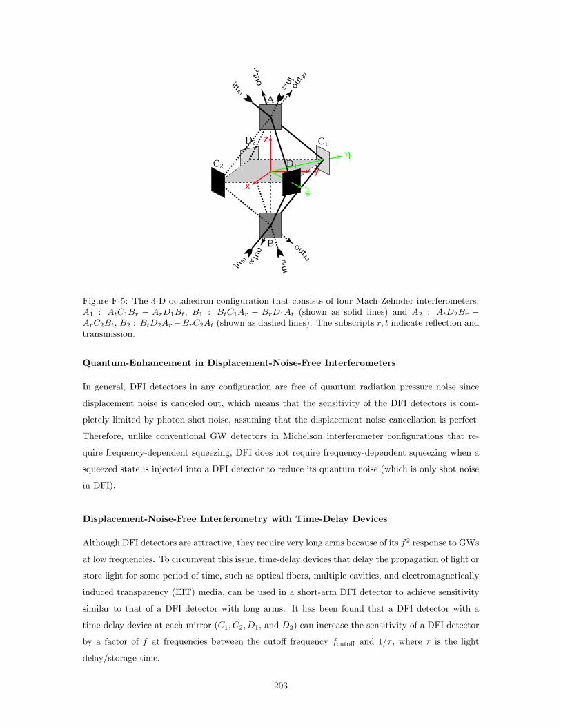
C1

C2

D2

A

B

x

z

inA

1

ou

tB

1

inA

2 ou

t B2

inB

2

outA

2

ou

tA

1

inB

1

D1y

Figure F-5: The 3-D octahedron configuration that consists of four Mach-Zehnder interferometers;A1 : AtC1Br − ArD1Bt, B1 : BtC1Ar − BrD1At (shown as solid lines) and A2 : AtD2Br −ArC2Bt, B2 : BtD2Ar −BrC2At (shown as dashed lines). The subscripts r, t indicate reflection andtransmission.

Quantum-Enhancement in Displacement-Noise-Free Interferometers

In general, DFI detectors in any configuration are free of quantum radiation pressure noise since

displacement noise is canceled out, which means that the sensitivity of the DFI detectors is com-

pletely limited by photon shot noise, assuming that the displacement noise cancellation is perfect.

Therefore, unlike conventional GW detectors in Michelson interferometer configurations that re-

quire frequency-dependent squeezing, DFI does not require frequency-dependent squeezing when a

squeezed state is injected into a DFI detector to reduce its quantum noise (which is only shot noise

in DFI).

Displacement-Noise-Free Interferometry with Time-Delay Devices

Although DFI detectors are attractive, they require very long arms because of its f2 response to GWs

at low frequencies. To circumvent this issue, time-delay devices that delay the propagation of light or

store light for some period of time, such as optical fibers, multiple cavities, and electromagnetically

induced transparency (EIT) media, can be used in a short-arm DFI detector to achieve sensitivity

similar to that of a DFI detector with long arms. It has been found that a DFI detector with a

time-delay device at each mirror (C1, C2, D1, and D2) can increase the sensitivity of a DFI detector

by a factor of f at frequencies between the cutoff frequency fcutoff and 1/τ , where τ is the light

delay/storage time.

203

Overview

In the following sections, a simple 3-D configuration that implements DFI without composite mir-

rors is discussed. First of all, Mach-Zehnder (MZ) interferometry is used so that laser noise can be

canceled right in the beginning. Moreover, each mirror participates in at least two MZ interferom-

eters, and thus has its location sensed redundantly. Finally, by combining the MZ output signals,

the redundant displacement information can be canceled out, leaving non-vanishing response to

GWs. In particular, it is shown that the 3-D configuration has ∼ f2 sensitivity at low frequencies,

which is the best one can achieve with DFI. A 3-D DFI configuration with time-delay devices is also

discussed. The details about the DFI and the DFI with time-delay devices can be found in Refs.

[25, 64] respectively.

F.4.2 Detector Description

The 3-D DFI detector configuration is shown in Fig. F-5. The mirrors are located on the eight

vertices of a regular octahedron with an edge length of 2L. All laser beams in the detector propagate

along the edges of the octahedron. A Cartesian coordinate system is attached to the octahedron,

with the origin coinciding with its center, the z axis coinciding with its B-A axis, the x axis in parallel

with the C1-D1 (D2-C2) direction, and the y axis in parallel with the C2-D1 (D2-C1) direction. ξ

and η are defined as shown in the figure. A balanced beamsplitter is located at each of vertices A

and B with normal directions in parallel with the x axis. The four perfectly reflective mirrors at

C1,2 and D1,2 are oriented such that the laser beams from A are reflected directly toward B. We

assume all the perfect mirrors to have an amplitude reflectivity of r = 1, and both beamsplitters to

have an amplitude reflectivity of −1/√

2 for the laser beams that travel from the +x side (traveling

toward the −x direction), and an amplitude reflectivity of +1/√

2 for the laser beams that travel

from the −x side. The edge lengths are assumed to be an integer multiple of the laser wavelength

in absence of laser noise, mirror motion, and GWs.

Likewise, four MZ interferometers can be constructed in a configuration as shown in Fig. F-5.

At the zero point, the output ports ( outA1,A2,B1,B2) are kept dark, while each input port is also the

bright port for another interferometer. During operations, for each MZ, I = A1, A2, B1, B2, if φ(t)I

and φ(r)I represent the additional phase shifts gained by the beams transmitted and reflected from

its first beamsplitter, respectively, then the output optical amplitude is proportional to

eiφ(t)I − eiφ(r)

I ∝ φ(t)I − φ(r)

I ≡ δφI . (F.20)

For interferometers A1 and A2, the first beamsplitter means A, while for B1 and B2, it means B. In

Eq. (F.20), we have a minus sign in front of eiφ(r)I , because light always incident from the +x side

of the beamsplitters with the first reflection always encounters a −1/√

2 reflectivity.

204

θ

ϕ

x

y

z

eX

eY

eZ

Figure F-6: The orthonormal system (eX , eY , eZ) used to describe a generic plane GW. eZ is thepropagation direction.

These additional phase shifts can arise from laser noise, displacement noise, and GWs. Because

we only consider linear order in GWs and the noises, we can first include only effects of laser and

displacement noises, construct a combination from the outputs of the four MZ interferometers that

is free from these noises, and then calculate its response to GWs. For dark-port detection, each MZ

is already free from laser noise, and therefore, we only need to consider displacement noise. For a

mirror with normal direction n and incident wavevector k, the phase shift gained by the reflected

light when the mirror moves spatially by δx is 2(n · k)(n · δx). For A1 and B1 interferometers, we

have

φ(t)A1

(t) =

√2ω

c[ηC1(t − 2L/c) + xB(t)] , (F.21)

φ(r)A1

(t) =

√2ω

c[ξD1(t − 2L/c) − xA(t − 4L/c)] , (F.22)

φ(t)B1

(t) =

√2ω

c[ηC1(t − 2L/c) + xA(t)] , (F.23)

φ(r)B1

(t) =

√2ω

c[ξD1(t − 2L/c) − xB(t − 4L/c)] , (F.24)

where ω is the laser frequency, c is the speed of light in vacuum, and ηC1 is the motion of C1 along

the η axis and so on. Thus, we have

δφA1 − δφB1 =[

φ(t)A1

− φ(r)A1

]

−[

φ(t)B1

− φ(r)B1

]

=

√2ω

c[xB(t) − xA(t) − xB(t − 4L/c) + xA(t − 4L/c)] . (F.25)

Note that motions of C1 and D1 are already canceled in this subtraction because the two MZs sense

their motions equally, due to the fact that |AD1| = |BD1| = |AC1| = |BC1| = 2L. Similarly, the

205

combination of the other two MZs is given by

δφA2 − δφB2 =

√2ω

c[xB(t) − xA(t) − xB(t − 4L/c) + xA(t − 4L/c)] . (F.26)

Consequently, the total combination

φDFI ≡ [δφA1 − δφB1 ] − [δφA2 − δφB2 ] (F.27)

is free from any displacement noise. This is also anticipated because A1 and A2 sense the beam-

splitters in the same way, and so do B1 and B2.

F.4.3 Detector Response to Gravitational Waves

The response of φDFI to GWs is calculated in this section. For a particular case with a plane GW

coming directly along the z axis such that eZ = ez in Eq. (1.5) and

hTT(t,x) = h(t − z/c) [eξ ⊗ eξ − eη ⊗ eη] , (F.28)

it is relatively simple to argue, based on the symmetry of the octahedron and the scheme of combining

the output signals from the interferometers, that the beams in all four branches or those involving

C1, D1, C2 and D2 respectively experience equal GW contributions. For the branch involving D1,

the response to GWs is given by

φGWDFI

ωL/c=

1

2

∫ 1

0dζ

h[t + (2Lζ −√

2L(1 − ζ))/c] + h[t + (2L(1 + ζ) +√

2Lζ)/c]

−h[t + (2Lζ +√

2L(1 − ζ))/c] − h[t + (2L(1 + ζ) −√

2Lζ)/c]

. (F.29)

In the frequency domain defined in Eq. (1.60), Eq. (F.29) becomes

φGWDFI(Ω) =

iωhe−i√

2ΩL/c

4Ω

(2 −√

2)[

1 − e(4+2√

2)iΩL/c]

+ (2 +√

2)[

e4iΩL/c − e2√

2iΩL/c]

, (F.30)

where φGWDFI and h are the Fourier transforms of φGW

DFI and h., and Ω is the GW frequency. Eq. (F.30)

shows a non-vanishing response to GWs.

For GWs with generic propagation directions and polarizations, the detector response to GWs

at low frequencies goes like ∼ f2 with

[

φGWDFI

]

ΩLc

,1=

4√

2

3

(

ΩL

c

)2 (ωL

c

)

[

h×(1 + cos2 θ) cos 2ϕ + 2h+ cos θ sin 2ϕ]

, (F.31)

where θ and ϕ are shown in Fig. F-6. For general frequencies and generic incoming GWs, the

206

10−2 10−1 100 101 10210−4

10−3

10−2

10−1

100

101

2Ω L/(π c)

|φDF

IG

W/(h

ω L

/c)|

Figure F-7: The response of the DFI detector to GWs. It is peaked when 2ΩL/(πc) ∼ 1 and decaysas ∼ f2 at low frequencies.

analytical formula for the transfer function is complicated, and therefore, not presented here.

F.4.4 Practicability of 3-D DFI Detectors

Without displacement noise, ideal DFI configurations are shot-noise-limited at all frequencies, and

therefore, the detector sensitivity can be improved by simply turning up the laser power. At fre-

quencies f > fc ≡ c/L, the 3-D configuration has comparable shot-noise-limited sensitivity to

conventional GW detector configurations with similar arm lengths and optical power, but without

optical cavities, at frequencies f < fc, the shot-noise-limited sensitivity degrades as (f/fc)2.

In practice, the effectiveness of displacement noise cancellation is limited by experimental im-

perfections. For example, the following requirements must be satisfied to optimize the performance

of DFI: (1) all interferometer arms have equal lengths, (2) beamsplitters are exactly 50/50, (3) mir-

rors are lossless, (4) beams incident on each mirror must all hit the same point. If a DFI detector

does not perfectly satisfy these requirements, it limits the displacement-noise reduction factor (in

amplitude) at max(δL/L, |RBS − TBS|, ε), where δL is the length accuracy, RBS and TBS are the

power reflectivity and transmissivity of the beamsplitters, and ε is the optical loss in the mirrors (in

power). It is reasonable to expect a 100 to 1000-fold reduction in displacement noise.

207

F.4.5 Utility of Time-Delay Devices in DFI Detectors

Although the DFI detector can evade displacement noise, it requires an arm length to be comparable

to the wavelength of GWs for detection since the detector response decays as f2 at low frequencies

up to the cutoff frequency

fcutoff =c

2L. (F.32)

The f2 response comes from the unique nature of the DFI detector with folded interferometer arms.

To decrease the f2 cutoff frequency, the DFI detector requires a very long arm, which is also a

requirement for Michelson-type GW detectors, but to detect an appreciable GW signal against

background displacement noise.

To circumvent this problem in DFI detectors, time-delay devices that delay the propagation of

light or store light for some period of time, such as optical fibers, multiple cavities, and electromag-

netically induced transparency (EIT) media, can be used in a short-arm DFI detector to achieve

sensitivity similar to that of a DFI detector with long arms. It has been found that a DFI detector

with a time-delay device at each mirror (C1, C2, D1, and D2) can increase the sensitivity of a DFI

detector by a factor of f at frequencies between the cutoff frequency fcutoff and 1/τ , where τ is the

light delay/storage time. Much of the derivation can be found in Ref. [64].

F.5 Quantitative Phase Imaging by Use of Stabilized Optical

Interferometry

F.5.1 Introduction

Optical microscopy has been the most commonly used method of investigation in medicine and

biology. Various related technologies have been developed over the past years [250]. Numerous

biological samples, including live cells, are quite transparent at visible wavelengths and behave es-

sentially as phase objects. Techniques such as phase contrast and Nomarski microscopy provide

contrast of nearly invisible samples by transforming the phase information into the intensity distri-

bution, thus revealing morphometric features of biological systems without the need for exogenous

contract agents [251]. However, the information obtained with these techniques about the phase

shift is only qualitative. Retrieving quantitative phase information from transparent objects with

high accuracy and low noise allows for novel applications in the biological investigation of structure

and dynamics [252]. Both interferometric [253, 254, 255] and non-interferometric [256] techniques

have been proposed for quantitative phase imaging of biological samples.

Recently, a stabilized Hilbert phase microscope as a quantitative phase imager with sub-nanometer

208

phase sensitivity and millisecond time resolution has been developed [255]. Its long-term stability

over extended periods of time allows for investigating the dynamics of biological systems on time

scales from seconds to a cell lifetime. Its high time resolution also enables investigation of many

processes that take place at the cellular level at kHz frequencies, including cytoskeletal dynamics

[257], cell membrane fluctuations [258], and neural activity [259]. In the next section, the stabilized

Hilbert phase microscope is introduced, and then, in the last section, measurement of cell membrane

tension using the microscope is carried out. The details of the microscope can be found in Ref. [255].

F.5.2 Stabilized Hilbert Phase Microscopy

A schematic of the Hilbert phase microscope is shown in Fig. F-8. The laser source is a He-Ne laser

at 632.8 nm. The laser is collimated and divided into the sample and reference arms to form a Mach-

Zehnder interferometer. The sample beam provides an illumination field for an inverted microscope

equipped with an immersion 100× objective with an NA of 1.2 that allows for a transverse resolution

of 0.26 µm. The tube lens is positioned such that the image of the sample is formed at the CCD

plane via the beamsplitter cube. The reference beam is collimated and expanded by a telescope that

consists of another microscope objective and recombined with the sample beam at the beamsplitter.

At the CCD plane, the reference beam can be approximated by a plane wave, which interferes with

the sample beam that contains the information of the sample.

The reference beam is purposely misaligned with respect to the sample beam such that uniform

fringes are created at an angle of 45 with respect to the x and y axes in the CCD detection plane,

such that for a given sample, the spatially varying irradiance at the image (CCD) plane across either

the x or y axis has the form

I(x) = IR + IS(x) + 2√

IRIS(x) cos[qx + φ(x)], (F.33)

where IR and IS(x) are the reference and sample irradiance distributions respectively, q is the

spatial frequency of the fringes, and φ(x) is the spatially varying phase associated with the object

(the quantity of interest in this microscope). The CCD (Hamamatsu Photonics C7770) has an

acquisition rate of 291 frames/s with 640×480 pixels per image and the fringes are sampled by

4-6 CCD pixels per period. High-pass filtering Eq. (F.33) gives I(x) = 2√

IRIS(x) cos[qx + φ(x)],

which is then demodulated at the spatial frequency q to obtain I(x) = 2√

IRIS(x) cosφ(x). Hilbert-

transforming the cosine function using the Kramers-Kronig relation

z(x) =1

2I(x) + i

P

2π

∫

I(x′

)

x − x′ dx′

(F.34)

209

CCD

Lens

Beamsplitter

Beamsplitter Sample

Objective

Objective

Pinhole

REFERENCEARM

SAMPLE ARMComputer

LASER

Fiber Fiber

Fiber

PD

Grating

LP HPMixerAdder PreAmp

HVAmp

LO

PZT

Lens

Figure F-8: A schematic of the stabilized Hilbert phase microscope in a Mach-Zehnder interferometerconfiguration that consists of a laser source, two balanced beamsplitters, two objectives, a sample,a tube lens, a pinhole, a photodetector (PD), a CCD camera, and an amplitude grating. Theinterference fringe spatially filtered by the grating is detected by the PD, high-pass filtered, amplified,and demodulated by a local oscillator (LO) that modulates the optical phase in the reference arm,yielding an error signal that is fed back to the interferometer via a piezo-electric transducer (PZT).

retrieves the phase information of the sample from a single-exposure image, given by

φ(x) = tan−1 Im[z(x)]

Re[z(x)]. (F.35)

In order to suppress fluctuations in relative phase between the two arms, a feedback control

system is used to lock the interferometer on an interference fringe. A small mirror in front of the

CCD deflects a portion of the interfering beams before they reach the CCD. At a plane conjugate to

the image (CCD) plane, an amplitude grating with the same period as the interferogram is placed.

Due to this spatial matching, each diffraction order n produced by the sample beam overlaps with

the order n − 1 of the reference beam. The interfering beams are spatially isolated by an aperture

and detected by a photodetector. The interference fringe is then detected by the PD, high-pass

filtered, amplified, and demodulated by a local oscillator (LO) that modulates the optical phase in

the reference arm, yielding an error signal that is fed back to the interferometer via a piezo-electric

transducer (PZT). The cutoff frequency of the high-pass filter is 1 kHz, the LO modulation frequency

is 15 kHz, and the cutoff frequency of the low-pass filter is 300 Hz.

The long-term stability of the microscope over extended periods of time due to the feedback

control system allows for investigating the dynamics of biological systems on time scales from seconds

210

to a cell lifetime. Its high time resolution due to the high sampling rate of the CCD also enables

investigation of many processes that take place at the cellular level at kHz frequencies.

F.5.3 Measurements of Cell Membrane Tension

The stabilized Hilbert phase microscope allows for transferring the information encoded in the phase

of the imaging field into the intensity distribution of the final image, and therefore, the optical phase

shift through a given sample can be regarded as a powerful endogenous contrast agent since it

contains information about both the thickness and refractive index of the sample. In this respect,

mature erythrocytes or red blood cells (RBCs) represent a very particular type of structure in that

they lack nuclei and major organelles, and hence, they can be modeled as optically homogeneous

objects and are useful for studying cell membranes, which have broad applications in both science

and technology [260, 261]. The RBC has a composite membrane that consists of a lipid bilayer

coupled to a two-dimensional spectrin network, which grants the cell its characteristic properties of

both softness and strong shear elasticity [262, 263].

The membrane tension of RBCs was measured by the stabilized Hilbert phase microscope, ana-

lyzed and compared with a theoretical model. The result is described in Ref. [255], and therefore,

will not be discussed any further here.

211

Bibliography

[1] A. Abramovici, W. Althouse, R. Drever, Y. Gursel, S. Kawamura, F. Raab, D. Shoemaker,

L. Sievers, R. Spero, K. Thorne, R. Vogt, R. Weiss, S. Whitcomb, and M. Zucker. Science,

256:325, 1992.

[2] B. Barish and R. Weiss. Phys. Today, 52:44, 1999.

[3] K. S. Thorne. In 300 Years of Gravitation. Cambridge University Press, Cambridge, 1987.

[4] L. Di Fiore and the VIRGO Collaboration. Class. Quant. Grav., 19:1421, 2002.

[5] B. Willke and the GEO Collaboration. Class. Quant. Grav., 19:1377, 2002.

[6] M. Ando and the TAMA Collaboration. Phys. Rev. Lett., 86:3950, 2001.

[7] Advanced LIGO. http://www.ligo.caltech.edu/advLIGO, 2001.

[8] D. F. Walls. Nature, 306:141, 1983.

[9] G. Breitenbach, S. Schiller, and J. Mlynek. Nature, 387:471, 1997.

[10] C. M. Caves. Phys. Rev. D, 23:1693, 1981.

[11] M. Xiao, L.-A. Wu, and H. J. Kimble. Phys. Rev. Lett., 59:278, 1987.

[12] R. E. Slusher, L. W. Hollberg, B. Yurke, J. C. Mertz, and J. F. Valley. Phys. Rev. Lett.,

55:2409, 1985.

[13] K. McKenzie, D. A. Shaddock, D. E. McClelland, B. C. Buchler, and P. K. Lam. Phys. Rev.

Lett., 88:231102, 2002.

[14] H. Vahlbruch, S. Chelkowski, B. Hage, A. Franzen, K. Danzmann, and R. Schnabel. Phys.

Rev. Lett., 95:211102, 2005.

[15] K. Goda, O. Miyakawa, E. E. Mikhailov, S. Saraf, R. Adhikari, R. Ward, K. McKenzie,

A. Weinstein, and N. Mavalvala. Submitted to Nature, 2007.

213

[16] K. Goda, E. E. Mikhailov, O. Miyakawa, S. Saraf, S. Vass, A. Weinstein, and N. Mavalvala.

arXiv:quant-ph/0703001, 2007.

[17] K. McKenzie, N. Grosse, W. P. Bowen, S. E. Whitcomb, M. B. Gray, D. E. McClelland, and

P. K. Lam. Phys. Rev. Lett., 93:161105, 2004.

[18] H. Vahlbruch, S. Chelkowski, B. Hage, A. Franzen, K. Danzmann, and R. Schnabel. Phys.

Rev. Lett., 97:011101, 2006.

[19] B. L. Schumaker and C. M. Caves. Phys. Rev. A, 31:3093, 1985.

[20] C. M. Caves and B. L. Schumaker. Phys. Rev. A, 31:3068, 1985.

[21] A. Einstein. Sitzungsberichte der Preussischen Akademie der Wissenschaften zu Berlin, 1915.

[22] A. Einstein. Annalen der Physik, 1916.

[23] A. Einstein. The Meaning of Relativity. Princeton University Press, 1922.

[24] S. L. Shapiro and S. A. Teukolsky. Black Holes, White Dwarfs, and Neutron Stars. Wiley-

Interscience, 1983.

[25] Y. Chen, A. Pai, K. Somiya, S. Kawamura, S. Sato, K. Kokeyama, R. L. Ward, K. Goda, and

E. E. Mikhailov. Phys. Rev. Lett., 97:151103, 2006.

[26] P. R. Saulson. Fundamentals of Interferometric Gravitational Wave Detectors. World Scientific,

1994.

[27] B. Abbott and the LIGO Scientific Collaboration. Phys. Rev. D, 69:122001, 2004.


[29] J. M. Weisberg and J. H. Taylor. Astrophys. J.

[30] J. H. Taylor, L. A. Fowler, and J. M. Weisberg. Nature, 277:437, 1979.

[31] R. A. Hulse and J. H. Taylor. Astrophys. J. Lett., 195:L51, 1975.



[34] G. G. Pavlov, D. Sanwal, and M. A. Teter. Proc. IAU Symp., 218:239, 2004.

[35] F. Haberl. Space Res., 33:638, 2004.

[36] D. I. Jones and N. Andersson. Mon. Not. R. Astron. Soc., 331:203, 2002.

214

[37] C. Van Den Broeck. Class. Quantum Grav., 22:1825, 2005.

[38] L. Bildsten. Astrophys. J., 501:L89, 1998.

[39] G. Ushomirsky, C. Cutler, and L. Bildsten. Mon. Not. R. Astron. Soc., 319:902, 2000.

[40] C. Cutler. Phys. Rev. D, 66:084025, 2002.

[41] A. Melatos and D. J. B. Payne. Astrophys. J., 623:1044, 2005.

[42] B. J. Owen. Phys. Rev. Lett., 95:211101, 2005.

[43] B. Abbott and the LIGO Scientific Collaboration. Phys. Rev. Lett., 94:181103, 2005.



[46] B. Abbott and the LIGO Scientific Collaboration. arXiv:gr-qc/0605028, 2006.



[49] T. Zwerger and E. Muller. Astron. Astrophys., 320:209, 1997.

[50] H. Dimmenlmeier, J. A. .Font, and E. Muller. Astrophys. J. Lett., 560:L163, 2001.

[51] B. Zhang and P. Meszaros. Int. J. Mod. Phys. A, 19:2385, 2003.

[52] B. Abbott and the LIGO Scientific Collaboration. Phys. Rev. Lett., 95:221101, 2005.

[53] M. Maggiore. Phys. Rep., 331:283, 2000.

[54] B. Abbott and the LIGO Scientific Collaboration. Astrophys. J., 659:918, 2007.

[55] B. Abbott and the LIGO Scientific Collaboration. arXiv:astro-ph/0703234, 2007.

[56] B. Abbott, the LIGO Scientific Collaboration, and ALLEGRO. Phys. Rev. D, 76:022001, 2007.


[58] R. R. Caldwell, R. A. Battye, and E. P. S. Shellard. Phys. Rev. D, 54:7146, 1996.

[59] J. Weber. Phys. Rev., 117:306, 1960.

[60] C. W. Misner, K. S. Thorne, and J. A. Wheeler. Gravitation. W. H. Freeman and Co., 1973.

[61] K. X. Sun, M. M. Fejer, E. G. Gustafson, and R. L. Byer. Phys. Rev. Lett., 76:16, 1996.

215

[62] C. S. Adams, M. Sigel, and J. Mlynek. Phys. Rep., 240:143, 1994.

[63] P. R. Berman. Atom Interferometry. Academic Press, 1997.

[64] K. Somiya, K. Goda, Y. Chen, and E. E. Mikhailov. Phys. Rev. D, 76:022002, 2007.

[65] F. A. E. Pirani. Acta Physica Polonica, 15:389, 1956.

[66] M. E. Gertsenshtein and V. I. Pustovoit. Soviet Physics - JETP, 16:433, 1963.

[67] R. Weiss. MIT Research Lab. of Electronics, Quarterly Progress Report No. 105, 1972.

[68] A. Bertolini, G. Cella, E. D’Ambrosio, R. DeSalvo, V. Sannibale, A. Takamori, and H. Ya-

mamoto. Gravitational Waves. Third Edoardo Amaldi Conference, 1999.

[69] K. Tsubono. Gravitational Wave Experiments. World Scientific, 1995.

[70] C. Casciano. Seismic Isolation for the Test Masses of the VIRGO Gravitational Wave Antenna.

Ph.D. Thesis, University of Pisa, 2002.

[71] G. Cella, R. DeSalvo, V. Sannibale, H. Tariq, N. Viboud, and A. Takamori. Nucl. Instrum.

Meth. A, 487:652, 2002.

[72] M. Barton, A. Bertolini, E. Black, G. Cella, E. Cowan, E. D’ambrosio, R. DeSalvo, K. Lib-

brecht, V. Sannibale, A. Takamori, N. Viboud, P. Willems, and H. Yamamoto. LIGO Internal

Working Note, LIGO-T990075-00, 1999.

[73] M. M. Fejer, S. Rowan, G. Cagnoli, D. R. M. Crooks, A. Gretarsson, G. M. Harry, J. Hough,

S. D. Penn, P. H. Sneddon, and S. P. Vyatchanin. Phys. Rev. D, 70:082003, 2004.

[74] K. Numata, A. Kemery, and J. Camp. Phys. Rev. Lett., 93:250602, 2004.

[75] G. M. Harry, A. M. Gretarsson, P. R. Saulson, S. E. Kittelberger, S. D. Penn, W. J. Startin,

S. Rowan, M. M. Fejer, D. R. M. Crooks, G. Cagnoli, J. Hough, and N. Nakagawa. Class.

Quantum Grav., 19:883, 2002.

[76] S. D. Penn, P. H. Sneddon, H. Armandula, J. C. Betzweiser, G. Cagnoli, J. Camp, D. R. M.

Crooks, M. M. Fejer, A. M. Gretarsson, G. M. Harry, J. Hough, S. E. Kittelberger, M. J.

Mortonson, R. Route, S. Rowan, and C. C. Vassiliou. Class. Quantum Grav, 20:2917, 2003.

[77] D. R. M. Crooks, G. Cagnoli, M. M. Fejer, A. M. Gretarsson, G. M. Harry, J. Hough, N. Nak-

agawa, S. Penn, R. Route, S. Rowan, and P. H. Sneddon. Class. Quantum Grav, 21:S1059,

2004.

[78] K. Numata, M. Ando, K. Yamamoto, S. Otsuka, and K. Tsubono. Phys. Rev. Lett., 91:260602,

2003.

216

[79] V. B. Braginsky, M. L. Gorodetsky, and S. P. Vyatchanin. Phys. Lett. A, 264:1, 1999.

[80] P. R. Saulson. Phys. Rev. D, 42:2437, 1990.

[81] Y. Levin. Phys. Rev. D, 57:659, 1988.

[82] H. J. Kimble, Y. Levin, A. B. Matsko, K. S. Thorne, and S. P. Vyatchanin. Phys. Rev. D,

65:022002, 2002.

[83] V. Giovannetti, S. Lloyd, and L. Maccone. Science, 306:1330, 2004.

[84] C. M. Caves. Phys. Rev. Lett., 45:75, 1980.

[85] W. Heisenberg. Zeitschrift fur Physik, 43:172, 1927.

[86] S. Weinberg. The Quantum Theory of Fields. Cambridge University Press, 1995.

[87] R. Loudon. The Quantum Theory of Light. Oxford University Press, 1973.

[88] D. F. Walls and G. J. Milburn. Quantum Optics. Springer-Verlag, Berlin, 1994.

[89] M. O. Scully and M. S. Zubairy. Quantum Optics. Cambridge, 1997.

[90] R. J. Glauber. Phys. Rev., 131:2766, 1963.

[91] B. Abbott and the LIGO Scientific Collaboration. Nucl. Instrum. Meth., A517:154, 2004.

[92] V. B. Braginsky and F. Ya. Khalili. Quantum Measurements. Cambridge University Press,

Cambridge, 1992.

[93] C. M. Caves, K. S. Thorne, R. W. P. Drever, V. D. Sandberg, and M. Zimmermann. Rev.

Mod. Phys., 52:341, 1980.

[94] K. Bencheikh, J. A. Levenson, P. Grangier, and O. Lopez. Phys. Rev. Lett., 75:3422, 1995.

[95] O. Miyakawa, R. Ward, R. Adhikari, M. Evans, B. Abbott, R. Bork, D. Busby, J. Heefner,

A. Ivanov, M. Smith, R. Taylor, S. Vass, A. Weinstein, M. Varvella, S. Kawamura, F. Kawazoe,

S. Sakata, and C. Mow-Lowry. Phys. Rev. D, 74:022001, 2006.

[96] A. Buonanno and Y. Chen. Phys. Rev. D, 64:042006, 2001.

[97] LIGO Sensitivities. http://www.ligo.caltech.edu/∼jzweizig/distribution/LSC−Data/, 2007.

[98] D. Sigg. LIGO-P980007-00-D, 1998.

[99] E. D’Ambrosio. Phys. Rev. D, 67:102004, 2003.

[100] R. O’Shaughnessy, S. Strigin, and S. Vyatchanin. arXiv:gr-qc/0409050v1, 2004.

217



[103] T. Corbitt, Y. Chen, and N. Mavalvala. Phys. Rev. A, 72:013818, 2005.

[104] J. Harms, R. Schnabel, and K. Danzmann. Phys. Rev. D, 70:102001, 2004.

[105] M. Matsuoka. Quantum Optics. University of Tokyo Press, 1996.

[106] S. M. Barnett and P. L. Knight. J. Opt. Soc. Am. B, 2:467, 1985.

[107] E. R. Pike and S. Sarkar. The Quantum Theory of Radiation. Oxford Science Publications,

1995.

[108] P. K. Lam, E. H. Huntington, T. R. Ralph, and H.-A. Bachor. Phys. Rev. Lett., 79:1471, 1997.

[109] T. C. Ralph and H.-A. Bachor. Opt. Commun., 110:301, 1995.

[110] A. Heidmann, R. J. Horowicz, S. Reynaud, E. Giacobino, C. Fabre, and G. Camy. Phys. Rev.

Lett., 59:2555, 1987.

[111] M. Fiorentino, P. L. Voss, J. E. Sharping, and P. Kumar. IEEE Photonics Technol. Lett.,

14:983, 2002.

[112] A. Furusawa, J. L. Sorensen, S. L. Braunstein, C. A. Fuchs, H. J. Kimble, and E. S. Polzik.

Science, 282:706, 1998.

[113] H. Yonezawa, T. Aoki, and A. Furusawa. Nature, 431:430, 2004.

[114] C. A. Sackett, D. Kielpinski, B. E. King, C. Langer, V. Meyer, C. J. Myatt, M. Rowe, Q. A.

Turchette, W. M. Itano, D. J. Wineland, and C. Monroe. Nature, 404:256, 2000.

[115] N. B. Grosse, W. P. Bowen, K. Mckenzie, and P. K. Lam. Phys. Rev. Lett., 96:063601, 2006.

[116] M. I. Kolobov. Rev. Mod. Phys., 71:1539, 1999.

[117] C. Fabre, J. B. Fouet, and A. Maitre. Opt. Lett., 25:76, 1999.

[118] N. Treps, U. Andersen, B. Buchler, P. K. Lam, A. Maitre, H.-A. Bachor, and C. Fabre. Phys.

Rev. Lett., 88:203601, 2002.

[119] C. H. Bennett, F. Bessette, G. Brassard, L. Salvail, and J. Smolin. J. Cryptography, 5:3, 1992.

[120] E. S. Polzik, J. Carri, and H. J. Kimble. Appl. Phys. B, 55:279, 1992.

[121] E. S. Polzik, J. Carri, and H. J. Kimble. Phys. Rev. Lett., 68:3020, Phys. Rev. Lett.

218

[122] P. Grangier, R. E. Slusher, B. Yurke, and A. LaPorta. Phys. Rev. Lett., 59:2153, 1987.

[123] A. G. White, P. K. Lam, D. E. McClelland, H.-A. Bachor, and W. J. Munro. J. Opt. B:

Quantum Semiclass. Opt., 2:553, 2000.

[124] F. A. A. El-Orany, M. S. Abdalla, and J. Perina. Euro. Phys. J. D, 41:391, 2006.

[125] T. Corbitt, Y. Chen, E. Innerhofer, H. Muller-Ebhardt, D. Ottaway, H. Rehbein, D. Sigg,

S. Whitcomb, C. Wipf, and N. Mavalvala. Phys. Rev. Lett., 98:150802, 2007.

[126] T. Corbitt, Y. Chen, F. Khalili, D. Ottaway, S. Vyatchanin, S. Whitcomb, and N. Mavalvala.

Phys. Rev. A, 73:023801, 2006.

[127] A. Dantan, M. Pinard, and P. R. Berman. Euro. Phys. J. D, 27:193, 2003.

[128] M. Fleischhauer, U. Rathe, and M. O. Scully. Phys. Rev. A, 46:5856, 1992.

[129] L.-A. Wu, H. J. Kimble, J. L. Hall, and H. Wu. Phys. Rev. Lett., 57:2520, 1986.

[130] R. W. Boyd. Nonlinear Optics. Academic Press, 2003.

[131] M. J. Collett and C. W. Gardiner. Phys. Rev. A, 30:1386, 1984.

[132] C. W. Gardiner and M. J. Collett. Phys. Rev. A, 31:3761, 1985.

[133] C. W. Gardiner. Phys. Rev. Lett., 70:2269, 1993.

[134] K. Goda, K. McKenzie, E. E. Mikhailov, P. K. Lam, D. E. McClelland, and N. Mavalvala.

Phys. Rev. A, 72:043819, 2005.

[135] A. G. White. Classical and Quantum Dynamics of Optical Frequency Conversion. Ph.D.

Thesis, The Australian National University, 1997.

[136] B. Yurke. Phys. Rev. A, 20:408, 1984.

[137] B. C. Buchler. Electro-optic Control of Quantum Measurements. Ph.D. Thesis, The Australian

National University, 2001.

[138] T. Aoki, G. Takahashi, and A. Furusawa. Opt. Express, 14:6930, 2006.

[139] S. Suzuki, H. Yonezawa, F. Kannari, M. Sasaki, and A. Furusawa. Appl. Phys. Lett., 89:061116,

2006.

[140] P. K. Lam. Applications of Quantum Electro-Optic Control and Squeezed Light. Ph.D. Thesis,

The Australian National University, 1996.

219

[141] W. P. Bowen. Experiments toward a Quantum Information Network with Squeezed Light and

Entanglement. Ph.D. Thesis, The Australian National University, 2003.

[142] P. K. Lam, T. C. Ralph, B. C. Buchler, D. E. McClelland, H.-A. Bachor, and J. Gao. J. Opt.,

1999.

[143] Y. Takeno, M. Yukawa, H. Yonezawa, and A. Furusawa. Opt. Express, 15:4321, 2007.

[144] Y. Yamamoto, S. Machida, and O. Nilsson. Phys. Rev. A, 24:4025, 1986.

[145] Y. Furukawa, K. Kitamura, A. Alexandrovski, R. K. Route, M. M. Fejer, and G. Foulon. Appl.

Phys. Lett., 78:1970, 2001.

[146] S. D. Smith, H. D. Riccius, and R. P. Edwin. Opt. Commun., 20:188, 1977.

[147] S. D. Smith, H. D. Riccius, and R. P. Edwin. Opt. Commun., 17:332, 1976.

[148] A. Yariv. Optical Electronics in Modern Communications. Oxford University Press, 1997.

[149] S. Somekh and A. Yariv. Appl. Phys. Lett., 6:301, 1972.

[150] S. Wang. Ph.D. Thesis, Royal Institute of Technology, 2005.

[151] T. Y. Fan, C. E. Huang, B. Q. Hu, R. C. Eckardt, Y. X. Fan, R. L. Byer, and R. S. Feigelson.

Appl. Opt., 26:2394, 1987.

[152] A. E. Siegman. Lasers. University Science Books, 1986.

[153] H. Kogelnik and T. Li. Appl. Opt., 5:1550, 1966.

[154] F. L. Pedrotti and L. S. Pedrotti. Introduction to Optics. Prentice Hall, 1989.

[155] E. E. Mikhailov, K. Goda, and N. Mavalvala. Phys. Rev. A, 74:033817, 2006.

[156] Y. Takeno, M. Yukawa, H. Yonezawa, and A. Furusawa. Opt. Express, 15:4321, 2007.

[157] P. Fritschel. LIGO Internal Working Note, G030460-00-R, 2003.

[158] P. Grangier, J. A. Levenson, and J-P. Poizat. Nature, 396:537, 1998.

[159] S. Chelkowski, H. Vahlbruch, B. Hage, A. Franzen, N. Lastzka, K. Danzmann, and R. Schnabel.

Phys. Rev. A, 71:013806, 2005.

[160] K. McKenzie, E. E. Mikhailov, K. Goda, P. K. Lam, N. Grosse, M. B. Gray, N. Mavalvala,

and D. E. McClelland. J. Opt. B: Quantum Semiclass. Opt., 7:S421, 2005.

[161] S. Chelkowski, H. Vahlbruch, K. Danzmann, and R. Schnabel. Phys. Rev. A, 75:043814, 2007.

220

[162] R. W. P. Drever, J. L. Hall, F. W. Kowalski, H. Hough, G. M. Ford, A. J. Munley, and

H. Ward. Appl. Phys. B, 31:97, 1983.

[163] C. Schori, J. L. Sorensen, and E. S. Polzik. Phys. Rev. A, 66:033802, 2002.

[164] J. Laurat, T. Coudreau, G. Keller, N. Treps, and C. Fabre. Phys. Rev. A, 70:042315, 2004.

[165] B. Abbott, G. Billingsley, L. Jones, R. Karwoski, J. Romie, M. Smith, D. Ugolini, S. Vass,

and A. Weinstein. LIGO Internal Working Note, LIGO-T010115, 2001.

[166] J. Rollins, D. Ottaway, M. Zucker, and R. Weiss. Opt. Lett., 29:1876, 2002.

[167] K. Wodkiewicz and M. S. Zubairy. Phys. Rev. A, 27:2003, 1983.

[168] D. D. Crouch and S. L. Braunstein. Phys. Rev. A, 38:4696, 1988.

[169] J. Gea-Banacloche and M. S. Zubairy. Phys. Rev. A, 42:1742, 1990.

[170] W. P. Bowen, R. Schnabel, N. Treps, H.-A. Bachor, and P. K. Lam. J. Opt. B: Quantum

Semiclass. Opt., 4:421–424, 2002.

[171] Y. T. Liu and K. S. Thorne. Phys. Rev. D, 62:122002, 2000.

[172] M. Cerdonio, L. Conti, A. Heidmann, and M. Pinard. Phys. Rev. D, 63:082003, 2001.

[173] L-A. Wu, S. F. Pereira, H. J. Kimble, and K. C. Peng. Phys. Rev. Lett., 68:3663, 1992.

[174] H. Vahlbruch, M. Mehmet, N. Lastzka, B. Hage, S. Chelkowski, A. Franzen, S. Goβler,

K. Danzmann, and R. Schnabel. arXiv:0706.1431, 2007.

[175] D. R. Weise, U. Strobner, A. Peters, J. Mlynek, S. Schiller, A. Arie, A. Skliar, and G. Rosen-

man. Opt. Commun., 184:329, 2000.

[176] G. M. Gibson, M. Ebrahimzadeh, M. J. Padgett, and M. H. Dunn. Opt. Lett., 23:397, 1999.

[177] A. Garashi, A. Arie, A. Skliar, and G. Rosenman. Opt. Lett., 23:1739, 1998.

[178] T. J. Edwards, G. A. Turnbull, M. H. Dunn., and M. Ebrahimzadeh. Opt. Express, 6:58, 2000.

[179] M. Ebrahimzadeh, G. A. Turnbull, T. J. Edwards, D. J. M. Stothard, I. D. Lindsday, and

M. H. Dunn. J. Opt. Soc. Am. B, 16:1499, 1999.

[180] A. Arie, G. Rosenman, A. Korenfeld, A. Skliar, M. Oron, M. Katz, and D. Eger. Opt. Lett.,

23:28, 1998.

[181] I. Juwiler, A. Arie, A. Skliar, and G. Rosenman. Opt. Lett., 24:1236, 1999.

[182] B. Dayan, A. Peer, A. A. Friesem, and Y. Silberberg. Phys. Rev. Lett., 94:043602, 2005.

221

[183] U. L. Andersen and P. Buchhave. Opt. Express, 10:887, 2002.

[184] T. Hirano, K. Kotani, T. Ishibashi, S. Okude, and T. Kuwamono. Opt. Lett., 30:1722, 2005.

[185] J. Laurat, T. Coudreau, N. Treps, A. Maitre, and C. Fabre. Phys. Rev. Lett., 91:213601, 2003.

[186] S. Feng and O. Pfister. Opt. Lett., 29:2800, 2004.

[187] B. Boulanger, M. M. Fejer, R. Blachman, and P. F. Bordui. Appl. Phys. Lett., 65:2401, 1994.

[188] T. A. Dricoll, H. J. Hoffman, R. E. Stone, and P. E. Perkins. J. Opt. Soc. Am. B, 3:683, 1986.

[189] W. R. Bosenberg and D. R. Guyer. Appl. Phys. Lett., 61:387, 1992.

[190] V. S. Chickarmane and G. S. Agarwal. Opt. Lett., 23:1132, 1998.

[191] T. Skauli, K. L. Vodopyanov, T. J. Pinguet, A. Schober, O. Levi, L. A. Eyres, M. M. Fejer,

J. S. Harris, B. Gerard, L. Becouarn, E. Lallier, and G. Arisholm. Opt. Lett., 27:628, 2002.

[192] I. Shoji, T. Kondo, A. Kitamoto, M. Shirane, and R. Ito. J. Opt. Soc. Am. B, 14:2268, 1997.

[193] E. E. Mikhailov, K. Goda, T. Corbitt, and N. Mavalvala. Phys. Rev. A, 73:053810, 2006.

[194] T. Corbitt, N. Mavalvala, and S. Whitcomb. Phys. Rev. D, 70:022002, 2004.

[195] D. Budker, D. F. Kimball, S. M. Rochester, and V. V. Yashchuk. Phys. Rev. Lett., 83:1767,

1999.

[196] M. D. Lukin, M. Fleischhauer, A. S. Zibrov, S. G. Robinson, V. L. Velichansky, L. Hollberg,

and M. O. Scully. Phys. Rev. Lett., 79:2959, 1997.

[197] S. E. Harris. Phys. Today, 50:36, 1997.

[198] H. Xia, A. J. Merriam, S. J. Sharpe, G. Y. Yin, and S. E. Harris. Phys. Rev. A, 59:3190, 1999.

[199] D. A. Braje, V. Balic, G. Y. Yin, and S. E. Harris. Phys. Rev. A, 68:041801, 2003.

[200] D. Akamatsu, K. Akiba, and M. Kozuma. Phys. Rev. Lett., 92:203602, 2004.

[201] M. Arikawa, K. Honda, D. Akamatsu, Y. Yokoi, K. Akiba, S. Nagatsuka, A. Furusawa, and

M. Kozuma. arXiv:0707.1971v1, 2007.

[202] E. E. Mikhailov, I. Novikova, Y. V. Rostovtsev, and G. R. Welch. Phys. Rev. A, 70:033806,

2004.

[203] A. V. Taichenachev, V. I. Yudin, R. Wynands, M. Stahler, J. Kitching, and L. Hollberg. Phys.

Rev. A, 67:033810, 2003.

222

[204] R. Wynands and A. Nagel. Appl. Phys. B, 68:1, 1999.

[205] G. Muller, M. Muller, A. Wicht, R.-H. Rinkleff, and K. Danzmann. Phys. Rev. A, 56:2385,

1997.

[206] M. Lukin, M. Fleischhauer, M. Scully, and V. L. Velichansky. Opt. Lett., 23(4):295, 1998.

[207] W. G. Unruh. Quantum Optics, Experimental Gravitation and Measurement Theory. Plenum,

New York, 1982.

[208] B. J. Meers. Phys. Rev. D, 38:2317, 1988.

[209] J. Mizuno, K. A. Strain, P. G. Nelson, J. M. Chen, R. Schilling, A. Rudiger, W. Winkler, and

K. Danzmann. Phys. Rev. Lett., 175:273, 1993.

[210] J. E. Mason. Signal Extraction and Optical Design for an Advanced Gravitational Wave

Interferometer. Ph.D. Thesis, California Institute of Technology, 2001.

[211] A. D. Michele, A. Weinstein, and D. Ugolini. LIGO Internal Working Note, LIGO-T010159-

00-R, 2001.

[212] F. Nocera. Class. Quantum Grav., 21:S481, 2004.

[213] R. M. Shelby, M. D. Levenson, S. H. Perlmutter, R. G. DeVoe, and D. F. Walls. Phys. Rev.

Lett., 59:691, 1987.

[214] S. Tanzilli, H. De Riedmatten, H. Tittel, H. Zbinden, P. Baldi, M. De Micheli, D. B. Ostrowsky,

and N. Gisin. Electron. Lett., 37:28, 2001.

[215] K. Sanaka, K. Kawahara, and T. Kuga. Phys. Rev. Lett., 86:5620, 2001.

[216] A. B. U’Ren, C. Silberhorn, K. Banaszek, and I. A. Walmsley. Phys. Rev. Lett., 93:093601,

2004.

[217] M. Fiorentino, C. Santori, S. M. Spillane, R. G. Beausoleil, and W. J. Munro. Phys. Rev. A,

75:032334, 2007.

[218] D. K. Armani, T. J. Kippenberg, S. M. Spillane, and K. J. Vahala. Nature, 421:925, 2003.

[219] K. J. Vahala. Nature, 424:839, 2003.

[220] T. J. Kippenberg, S. M. Spillane, and K. J. Vahala. Phys. Rev. Lett., 93:083904, 2004.

[221] C. Caloz, C. C. Chang, and T. Itoh. J. Appl. Phys., 90:11, 2001.

[222] G. V. Eleftheriades, A. K. Iyer, and P. C. Kremer. IEEE Trans. on Microwave Theory and

Techniques, 50:2702, 2002.

223

[223] A. Grbic and G. V. Eleftheriades. Phys. Rev. Lett., 92:117403, 2004.

[224] N. Fang, H. Lee, C. Sun, and X. Zhang. Science, 308:534, 2005.

[225] A. K. Popov, V. V. Slabko, and V. M. Shalaev. Laser Phys. Lett., 3:293, 2006.

[226] A. K. Popov and V. M. Shalaev. Opt. Lett., 31:2169, 2006.

[227] M. W. Klein, M. Wegener, N. Feth, and S. Linden. Opt. Express, 15:5238, 2007.

[228] M. W. Klein, C. Enkrich, M. Wegener, and S. Linden. Science, 313:502, 2006.

[229] National Institute of Standards and Technology. http://physics.nist.gov/cuu/Constants, 2007.

[230] Lawrence Berkeley National Laboratory. http://www.lbl.gov, 2007.

[231] CERN. http://public.web.cern.ch/Public/Welcome.html, 2007.

[232] Almaz Optics Inc. http://www.almazoptics.com/KTP.htm, 2007.

[233] P. Horowitz and W. Hill. The Art of Electronics. Cambridge University Press, 1989.

[234] Mini-Circuits. http://www.minicircuits.com, 2007.

[235] V. S. Ilchenko, A. A. Savchenkov, A. B. Matsko, and L. Maleki. Phys. Rev. Lett., 92:043903,

2004.

[236] A. A. Savchenkov, V. S. Ilchenko, A. B. Matsko, and L. Maleki. Phys. Rev. A, 70:051804,

2004.

[237] M. L. Gorodetsky, A. D. Pryamikov, and V. S. Ilchenko. J. Opt. Soc. Am. B, 17:1051, 2000.

[238] A. A. Savchenkov, A. B. Matsko, D. Strekalov, M. Mohageg, V. S. Ilchenko, and L. Maleki.

Phys. Rev. Lett., 93:243905, 2004.

[239] J. M. Geary. Introduction to Wavefront Sensors. SPIE Press, Bellingham, Washington, 1995.

[240] R. V. Shack and B. C. Platt. J. Opt. Soc. Am., 61:656, 1971.

[241] E. Morrison, B. J. Meers, D. I. Robertson, and H. Ward. Appl. Opt., 33:5037, 1994.

[242] Y. Hefetz, N. Mavalvala, and D. Sigg. J. Opt. Soc. Am. B, 14:1597, 1997.

[243] G. Mueller, Q. Shu, R. Adhikari, D. B. Tanner, D. Reitze, D. Sigg, N. Mavalvala, and J. Camp.

Opt. Lett., 25:266, 2000.

[244] K. Goda, D. Ottaway, B. Connelly, R. Adhikari, N. Mavalvala, and A. Gretarsson. Opt. Lett.,

29:1452, 2004.

224

[245] P. Fritschel, R. Bork, G. Gonzalez, N. Mavalvala, D. Ouimette, H. Rong, D. Sigg, and

M. Zucker. Appl. Opt., 40:4988, 2001.

[246] P. Fritschel, N. Mavalvala, D. Shoemaker, D. Sigg, M. Zucker, and G. Gonzalez. Appl. Opt.,

37:6734, 1998.

[247] J. Betzwieser, K. Kawabe, and L. Matone. LIGO Internal Working Note, LIGO-T040156-00-D,

2004.

[248] S. Kawamura and Y. Chen. Phys. Rev. Lett., 93:211103, 2004.

[249] Y. Chen and S. Kawamura. Phys. Rev. Lett., 96:231102, 2006.

[250] D. J. Stephens and V. J. Allan. Science, 300:82, 2003.

[251] F. Zernike. Science, 121:345, 1955.

[252] C. Yang, A. Wax, M. S. Hahn, K. Badizadegan, R. R. Dasari, and M. S. Feld. Opt. Lett.,

26:1271, 2001.

[253] T. Ikeda, G. Popescu, R. R. Dasari, and M. S. Feld. Opt. Lett., 30:1165, 2005.

[254] G. Popescu, T. Ikeda, C. A. Best, K. Badizadegan, R. R. Dasari, and M. S. Feld. J. Biomed.

Opt., 10:060503, 2005.

[255] G. Popescu, T. Ikeda, K. Goda, C. A. Best-Popescu, M. Laposata, S. Manley, R. R. Dasari,

K. Badizadegan, and M. S. Feld. Phys. Rev. Lett., 97:218101, 2006.

[256] D. Paganin and K. A. Nugent. Phys. Rev. Lett., 80:2586, 1998.

[257] L. Miao, O. Vanderline, M. Stewart, and T. M. Roberts. Science, 300:1405, 2003.

[258] A. E. Pelling, S. Sehati, E. B. Gralla, J. S. Valentine, and J. K. Gimzewski. Science, 305:1147,

2004.

[259] D. A. Dombeck, M. Blanchard-Desce, and W. W. Webb. J. Neurosci, 24:299, 2004.

[260] R. Lipowsky. Nature, 349:475, 1991.

[261] E. Sackmann. Science, 271:43, 1996.

[262] D. Boal. Mechanics of the Cell. Cambridge University Press, Cambridge, England, 2002.

[263] R. M. Hochmuth and R. E. Waugh. Annual Review of Physiology, 49:209, 1987.

225

development of techniques for quantum-enhanced laser

Documents