development of thermal sprayed tube and mesh heat

Development of thermal sprayed tube and mesh

heat exchangers for waste heat recovery

by

Xuerui Han

A thesis submitted in partial fulfillment of the requirements for the degree of

Master of Science

Department of Mechanical Engineering

University of Alberta

© Xuerui Han, 2020

ii

Abstract

Development of a lab-scale heat exchanger with increased mesh to tube contact area was

accomplished by flattening tubing prior to attaching wire mesh. This novel heat exchanger

prototype utilizes thermal sprayed coating to attach wire mesh onto tubing surfaces instead of

conventional brazing or welding of extended surfaces. Twin wire arc spray equipment was utilized

to deposit stainless steel coating onto stainless steel mesh and tube. Four samples with varied

coating thicknesses and spray deposition settings were fabricated to be compared with an

unmeshed sample to quantify the heat transfer enhancement of the mesh.

A simple heated wind tunnel was designed in tandem with the lab scale prototype. Air propelled

by axial fan towards the sample placed inside a rectangular duct, is heated by a propane torch,

mimicking the environment at the exhaust of flare or flue gas stacks. Steady state inlet and outlet

water temperatures were measured. For heat transferred into the water, meshed and coated samples

performed 38% to 217% better than bare tube. Temperature difference trends were in line with

previous studies but magnitudes were 1.5 to 4 times greater, demonstrating the heat transfer

enhancement from wire mesh, flattened tube, and thicker coatings.

A fin model is developed to quantify the heat transfer from mesh wires and integrated into a

discretized energy balance to predict outlet temperatures a priori and quantify thermal resistances

in each sample. The results of the model indicate that coating thickness has the largest impact on

thermal resistance, with values at least 1 or 2 orders of magnitude greater than other thermal

resistances in the heat transfer network of the lab scale meshed tubular heat exchangers. The fin

temperature distribution also exhibits small lengths of temperature variation along the fin, meaning

future designs need not utilize fins longer than 4 mm, showing potential reductions in material,

weight and size without impacting performance.

iii

Acknowledgements

Without the following people who have assisted me along the way, this degree would hardly have

been possible. I would like to thank my supervisors Dr. André McDonald and Dr. Sanjeev Chandra

for their guidance and support throughout my research. You have been invaluable in teaching me

the approach to research, defining the problem, designing an experiment, gathering data, making

sense of data, and presenting useful and intelligent information to the academic community.

During my collaboration and visit to the University of Toronto for sample fabrication, I would like

to extend a warm thank you to all the support I received from the Centre for Advanced Coating

Technologies staff and colleagues. Thank you for welcoming me during my stay, sharing the lab

space / equipment, as well as teaching me the ropes. In particular I would like to thank Dr. Larry

Pershin, Jordan Bouchard, and Sudarshan Devaraj.

During the experimentation phase at the University of Alberta Protective Clothing and Equipment

Research Facility, I am grateful for all the support and enthusiasm that Mr. Stephen Paskaluk

provided. Many of the troubleshooting fixes that you delivered allowed me to resume my data

collection. Thank you for maintaining a safe work environment for the duration of my experiments.

It is with the input of the many brilliant staff at the University of Alberta Mechanical Engineering

machine shop that much of my designs were brought to reality. In particular, I would like to thank

Daniel Mooney, Rick Conrad, and Wade Parker for their seemingly infinite patience with my

repeated design consultations, tool borrowing, and machining requests.

Lastly, I would like to sincerely appreciate my friends and family for supporting me throughout

this endeavor. Thanks to Ojaswi Dhoubhadel and Usama Asad, for gifting me with endless

laughter and adventure. Dillon Lee for your deep care and the countless occasions where you lifted

my spirits and listened to my predicaments. My parents, who encouraged and supported me even

when I doubted myself. My colleagues Jacob John, Adekunle Ogunbadejo, and Guriqbal Munday

who were always eager to listen and help and made the tougher days easier.

The heart of man plans his way, but the Lord establishes his steps. Prov. 16:9

iv

Contents Abstract _____________________________________________________________________ ii

Acknowledgements ____________________________________________________________ iii

List of Tables _______________________________________________________________ vii

List of Figures _______________________________________________________________ viii

Nomenclature ________________________________________________________________ x

1 Introduction ______________________________________________________________ 1

1.1 Heat exchanger types and classifications ____________________________________ 1

1.2 Low grade waste heat recovery ___________________________________________ 3

1.3 Thermal sprayed coating ________________________________________________ 4

1.4 Novel thermal sprayed heat exchanger _____________________________________ 5

1.5 Spray-on-mesh for low grade heat recovery _________________________________ 6

1.6 Objectives ____________________________________________________________ 8

1.7 Thesis organization ____________________________________________________ 8

2 Lab-scale meshed tubular heat exchanger design and fabrication ___________________ 10

2.1 Design of lab-scale heat exchangers ______________________________________ 10

2.1.1 Tubing machining method __________________________________________ 10

2.1.2 Wire mesh selection _______________________________________________ 12

2.1.3 Mesh clamping method _____________________________________________ 13

2.2 Experimental Method __________________________________________________ 16

2.2.1 Wire-arc spray fabrication __________________________________________ 16

3 Mathematical model for lab-scale heat exchanger heat transfer heat transfer analysis ____ 19

3.1 Discretized heat exchanger energy balance _________________________________ 19

3.2 Defining all components of 𝑞fin for each discretized segment __________________ 20

3.3 Solving the 1st order linear differential equation _____________________________ 22

4 Application of lab-scale heat exchangers in heated air tests ________________________ 24

4.1 Design of simple heated wind tunnel ______________________________________ 24

4.1.1 Fan and duct design _______________________________________________ 24

4.1.2 Heating source for duct _____________________________________________ 25

4.2 Experimental method __________________________________________________ 27

4.2.1 Fan and propane torch operation______________________________________ 27

4.2.2 Hydraulic system configuration ______________________________________ 27

v

4.2.3 Temperature measurement __________________________________________ 28

5 Results and Discussion ____________________________________________________ 30

5.1 Steady state measurements ______________________________________________ 30

5.1.1 Water temperature difference at four flowrate set points ___________________ 30

5.1.2 Air temperature measurements _______________________________________ 30

5.2 Flow characterization in lab-scale heat exchangers ___________________________ 33

5.2.1 Rate of heat transfer in heat exchangers ________________________________ 33

5.2.2 Internal flow heat transfer coefficient __________________________________ 35

5.2.3 External flow heat transfer coefficient _________________________________ 37

5.3 Application of discretized mesh and tube heat exchanger model ________________ 38

5.3.1 Solving for wire mesh fin heat transfer coefficient in discretized model _______ 38

5.3.2 Prediction of outlet water temperature with average air side heat transfer

coefficient in discretized model ______________________________________________ 40

5.4 One-dimension heat transfer Biot approximation ____________________________ 41

5.5 Infinite fin approximation and effective fin length ___________________________ 42

5.6 Coating thickness _____________________________________________________ 44

5.6.1 Coating cross section ______________________________________________ 44

5.7 Thermal sprayed coating conductive resistance ______________________________ 47

5.7.1 Effects of high temperature gradient areas due to high thermal resistances _____ 50

5.8 Heat transfer rate for finned vs. bare tube heat exchangers _____________________ 52

6 Conclusions and future work ________________________________________________ 54

6.1 Conclusion __________________________________________________________ 54

6.2 Future work _________________________________________________________ 55

6.2.1 Improvements on sources of measurement uncertainty / error _______________ 55

6.2.2 Improvements on testing capability ___________________________________ 56

6.2.3 Improvements on mathematical modelling ______________________________ 56

6.2.4 Future investigation into coating thermal resistances ______________________ 57

6.2.5 Future design considerations for mesh fins _____________________________ 57

References __________________________________________________________________ 58

Appendix A _________________________________________________________________ 61

A.1 Industrial-scale prototype heat exchanger design for industrial waste heat recovery _ 61

i. Prototype heat exchanger description _____________________________________ 61

ii. Prototype heat exchanger test cart design __________________________________ 63

vi

iii. Hydraulic system sizing and calculation _________________________________ 65

iv. Air flow control and measurement system design __________________________ 67

A.2 Hydraulic design calculations for industrial-scale prototype ____________________ 69

A.3 Application of industrial-scale prototype heat exchanger ______________________ 73

i. Experimental Method __________________________________________________ 73

ii. Results and Discussion _________________________________________________ 78

iii. Overall summary of tests _____________________________________________ 83

A.4 Circulator pump performance curves ______________________________________ 85

A.5 Simulated results of flue gas prototype heat exchanger tests ____________________ 85

Appendix B _________________________________________________________________ 88

B.1 Drawings for tube bending, tube press, and assembly process __________________ 88

vii

List of Tables

Table 1: Wire arc spray parameters (settings for best coating as defined in previous work [29]) ............................. 17 Table 2: Fin temperature distribution and heat transfer rate equations ..................................................................... 21 Table 3: Inlet and outlet water temperature measurements for each sample at four flowrates .................................. 30 Table 4: Crossflow air temperature and speed measurement ..................................................................................... 31 Table 5: Bare tube heat exchanger fluid properties and water side heat transfer coefficient ..................................... 36 Table 6: Bare tube heat exchanger heat transfer resistances and heat transfer coefficients ...................................... 38 Table 7: Model predicted heat transfer coefficients for meshed heat exchangers assuming perfect fin to tube contact

..................................................................................................................................................................................... 39 Table 8: Apparent average heat transfer coefficients for meshed heat exchangers and predicted outlet temperature

accuracy ...................................................................................................................................................................... 41 Table 9: All samples produced and corresponding coating thicknesses ..................................................................... 44 Table 10: Polishing settings for sample preparation (machine specific) .................................................................... 45 Table 11: Temperature difference and coating conductive resistance between base of mesh fins and heat exchanger

tube relative to thick coating sample (modeled as perfect contact) ............................................................................. 49 Table 12: Comparison of thermal resistance values in the heat exchanger thermal resistance network .................... 50 Table 13: Average heat transfer rate comparison table .............................................................................................. 52 Table 14: Chronological iterations of prototype heat exchanger test cart .................................................................. 64 Table 15: Operational flow rates and friction losses for various diameter hydraulic systems ................................... 69 Table 16: Loss coefficients for various hydraulic components .................................................................................... 70 Table 17: Flue gas heat exchanger test results for three water flow rates .................................................................. 79 Table 18: Summary Table for Prototype Heat Exchanger Performance Tests ............................................................ 83

viii

List of Figures

Figure 1: Four possible flow configurations of heat exchangers: (1) counter flow, (2) parallel flow, (3) cross-flow,

(4) hybrid [2] ________________________________________________________________________________ 1 Figure 2: Heat exchanger categories ______________________________________________________________ 2 Figure 3: Rezaey (Left) and Fu (Right) lab scale samples [28], [30] ____________________________________ 10 Figure 4: Tube dimensions round (Left) and flattened (Right) __________________________________________ 11 Figure 5: Bent and flattened bare tube heat exchanger _______________________________________________ 12 Figure 6: Welded mesh sample [43]______________________________________________________________ 13 Figure 7: Woven mesh sample [44] ______________________________________________________________ 13 Figure 8: Two wire mesh clamping methods, wire tie method (L) compared with screw and nut method (R) with

partial masking by aluminum foil to protect screw threads from coating deposition _________________________ 14 Figure 9: Various sample masking tests, heat resistant tape (Top Left), tape melted onto mesh after spraying (Top

Right), Aluminum foil over tap (Bottom Left), and Aluminum sheet secured with wire (Bottom Right) ___________ 15 Figure 10: Heat exchanger tube with wire mesh fastened by screws and nuts, masked with aluminum sheet, hung

from sample holder with wire, tube ends protected with masking tape ___________________________________ 16 Figure 11: Rectangular shape spray torch trajectory (Left) and linear torch trajectory (Right) ________________ 17 Figure 12: Energy Balance Conceptualization _____________________________________________________ 19 Figure 13: Energy balance for infinitesimal section of finned heat exchanger _____________________________ 19 Figure 14: Unit cell section of heat exchanger (L) and three consecutive H-EX segments with different colored fins

(R) ________________________________________________________________________________________ 20 Figure 15: Heat exchanger tube cross section with fins labeled 1 through 4 ______________________________ 21 Figure 16: Heat exchanger segments with length labeled _____________________________________________ 22 Figure 17: Duct drawing and detailed views of slot, sample fitment, and torch insertion _____________________ 25 Figure 18: Propane torch flames reaching the outlet of the duct (Left), Propane torch head sealed into duct port

with heat resistant foil tape (Right) ______________________________________________________________ 26 Figure 19: Liquid system of lab scale heat exchanger test setup ________________________________________ 28 Figure 20: Duct cross section measurement points (red dots) for air pressure and temperature, Pitot tube and

thermocouple probe used for measurements (Bottom Left) ____________________________________________ 29 Figure 21: Temperature difference plot for all samples at four flow rates ________________________________ 32 Figure 22: Thermal resistance network associated with heat transfer in a double-pipe heat exchanger [45] _____ 33 Figure 23: Table of Nusselt numbers for various tube cross sections [45] ________________________________ 35 Figure 24: Entrance length and overall dimensions of lab scale meshed heat exchanger _____________________ 37 Figure 25: Temperature distribution along longitudinal fin, thinly coated (<1 mm) sample __________________ 43 Figure 26: Temperature distribution along longitudinal fin, medium thickness (>1 mm) coating ______________ 44 Figure 27: Various tube, coating and mesh wire cross sections: high speed rectangular trajectory thin coating with

extended gaps (Top Left), high speed rectangular trajectory thin coating with void between tube and wire (Top

Right), low speed linear trajectory medium coating with void (Bottom Left), and low speed rectangular trajectory

thick coating with void (Bottom Right) ____________________________________________________________ 45 Figure 28: Thermal resistance network for meshed tubular heat exchanger _______________________________ 47 Figure 29: Unevenly heated center of wire mesh heat exchanger _______________________________________ 51 Figure 30: Coating delamination from tube surface, showing gap between mesh and tube ___________________ 51 Figure 31: Specification for prototype heat exchanger constructed by Rezaey and Chandra [28] ______________ 62 Figure 32: Original prototype mounting design - seated within stack, isometric view (Top) and top-down view

(Bottom) ___________________________________________________________________________________ 62 Figure 33: Wire mesh mounting prior to wire-arc coating and bonding __________________________________ 63 Figure 34: Staggered Meshed and Unmeshed Sandwich Design for Comparative Testing ____________________ 63 Figure 35: Final portable test cart for prototype heat exchanger _______________________________________ 65 Figure 36: Header pipe fluid distribution _________________________________________________________ 66 Figure 37: Fluid system - proposed design for pump sizing ____________________________________________ 67 Figure 38: Schematic of testing setup for hot flue gas - cold water test ___________________________________ 68

ix

Figure 39: Heat Exchanger Single Tube Path Schematic _____________________________________________ 72 Figure 40: Photograph of hot flue gas - cold water test setup __________________________________________ 75 Figure 41: Torch tip trajectory across heat exchanger prototype _______________________________________ 76 Figure 42: Flame used for heating passes _________________________________________________________ 77 Figure 43: Large vane axial fan for air cooling tests _________________________________________________ 78 Figure 44: 500 mm/s robot speed flame spray heating _______________________________________________ 80 Figure 45: 1500 mm/s robot speed flame spray heating ______________________________________________ 80 Figure 46: 4.02 GPM cool air test temperature log __________________________________________________ 82 Figure 47: 6.85 GPM cool air test temperature log __________________________________________________ 82 Figure 48: 8.14 GPM cool air test temperature log __________________________________________________ 82 Figure 49: Main screen of Coil program graphical user interface ______________________________________ 86 Figure 50: Input for calculating TWH flue gas heating scheme for prototype heat exchanger _________________ 87 Figure 51: Output results of simulated prototype heat exchanger _______________________________________ 87

https://d.docs.live.net/32cf55e4235838cf/Desktop/Han_Thesis%20Draft%20v5.docx#_Toc49283428

x

Nomenclature

A area, m2

Bi Biot number, dimensionless

Cp specific heat at constant pressure, J/kg K

D diameter, m

e exponential, dimensionless

f friction factor, dimensionless

h convection heat transfer coefficient, W/m2 K

k thermal conductivity, W/m K

L length, m

ṁ mass flow rate, kg/s

Nu Nusselt number, dimensionless

P Perimeter, m

Pr Prandtl number, dimensionless

q̇ heat transfer rate, W

R thermal resistance, °C /W

Re Reynolds number, dimensionless

U overall heat transfer coefficient, W/m2 K

T temperature, °C

x distance, m

xi

Greek Symbols

∆ delta, difference

δ characteristic length, m

π pi

ρ density, kg/m3

∞ ambient

Subscripts

b base

c cross-section

fin mesh wire fin

h entrance length

i inner

o outer

s surface

tube bare tube

w water

1

1 Introduction

1.1 Heat exchanger types and classifications Heat exchangers transfer heat between two or more fluids. They can range in size from microscale

heatsinks used for cooling microchips up to cooling towers which can be several hundred meters

tall. Heat exchangers are useful in heating, cooling, and energy recovery processes. If the fluids

are kept separate, heat exchangers are commonly categorized into four main types by their flow

configuration: counter flow, parallel flow, crossflow, and hybrids of the previous types [1]. The

diagram below depicts each flow type. Note that while some diagrams depict single-pass flow,

multi-pass configurations do exist, especially for the hybrid flow configurations.

(1) (2)

(3) (4)

Figure 1: Four possible flow configurations of heat exchangers: (1) counter flow, (2) parallel flow, (3) cross-flow, (4) hybrid [2]

Another method to characterize heat exchangers is by dividing them into recuperative or

regenerative [3]. Recuperative heat exchangers work by having at least two concurrently flowing

fluids move within the heat transfer volume. Regenerative heat exchangers use one flow path,

alternating between hot and cold fluid flows. Regenerative heat exchangers can be dynamic or

static depending on if the component passing the heat is stationary or moving.

2

Recuperative heat exchangers can be further classified by whether there is fluid contact or not.

Indirect recuperative heat exchangers do not place the fluids in contact with each other and a wall,

tube, or other impermeable membrane prevents mixing [4]. Direct recuperative heat exchangers

put two fluids together with mixing by design as part of the heat transfer process, examples include

steam injectors or cooling towers. The mixed fluids may or may not be miscible and one of the

fluids may not be recovered in the heat transfer process. The figure below organizes the

aforementioned heat exchangers into a hierarchical diagram. The focus of this thesis is on indirect

recuperative heat exchangers.

Figure 2: Heat exchanger categories

Indirect recuperative heat exchangers have several working principles, one type uses fluid flowing

in concentric pipes (Double-Pipe), others have tube banks enclosed in a shell (Shell-and-Tube),

and yet another approach uses plate-fins which are attached to the tubes in order to enhance heat

transfer performance by increasing surface area [5].

Heat transfer in heat exchangers depends on a multitude of factors such as: heat transfer

coefficients of tube material and fluids, fluid flow rates, fluid flow characteristics, surface

geometry, extended surfaces, and heat transfer area. Conventional plate-fin exchangers utilize thin

fins attached to bare tubes with welding or brazing methods to increase the heat transfer surface

area [6].

The novel thermally sprayed heat exchangers covered in this thesis are derived from the

aforementioned indirect recuperative type heat exchanger. Instead of conventional joining methods

such as welding or brazing, these spray-on-mesh crossflow heat exchangers utilize wire mesh

Heat Exchangers

Recuperative

Indirect

Direct

Renegerative

Dynamic

Static

3

bonded to the tube surfaces with a thermal sprayed coating process. A proposed usage case for

these tubular heat exchangers is waste heat recovery.

1.2 Low grade waste heat recovery The oil and gas industry in Alberta accounts for over 80% of Canada’s crude oil production [7]. A

necessary component of natural resources extraction, transport and refining is flaring. The energy

sector uses flares to safely vent poisonous and/or combustible volatile organic compounds (VOCs)

which are an unusable or not captured as a byproduct from a multitude of upstream to downstream

processes. It may be uneconomical to store or process these VOC byproducts. These exhausts are

controversial due to their highly visible smoke, steam or flame emissions which could be a visual

indicator of greenhouse gas and/or pollutant release into the atmosphere. Release of VOCs directly

into the atmosphere without combusting them into carbon dioxide and water can be more harmful

to the environment.

Flare stack discharge temperatures are typically around 500 to 1100 degrees Celsius [8], [9]. Flue

gas chimneys are present to exhaust combustion end product. Cooling towers are ubiquitous in

many facilities in order to dissipate waste heat generated by industrial processes. By harnessing

these sources of waste heat to preheat feedstock or water for existing processes, operators can

reduce the energy demand and ultimately, carbon emissions can be cut down.

Energy recovered by a heat exchanger integrated into an organic Rankine cycle (ORC), electricity

can be generated via turbine, further reducing carbon footprints by capturing energy from waste

heat sources. A literature review by Mondejar, et al. showed that ORC systems had the potential

to create 15% in fuel savings in diesel powered cargo ships [10]. A case study by Khatita, et al.

examines how different working fluids and operating conditions in an oil and gas plant in Egypt

would provide the best profitability, confirming that waste heat energy recapture is economically

feasible [11]. Lastly, Mudasar, et al. showed that a biogas fueled ORC was “an efficient solution

for domestic scale power generation applications in rural areas [12].”

Unfortunately, flue gas and flare stacks present difficult operating conditions due to extreme

temperatures, rapid temperature changes, fouling agents from incomplete combustion,

carburization, and corrosive gas mixtures. It has been shown in real world case study, with the

right conditions, such as heat, humidity, carbide precipitation, metals used in flare tips are

susceptible to cracking from intergranular corrosion from a condition known as sensitization [13].

4

Other elements such as sulfur can also attack the metal by embedding ions within the material

causing corrosion. The usage of thermally sprayed coatings in order to protect stainless steel flare

tips from sulfidation and prolong service life has been successfully demonstrated in industry in a

Saudi Aramco study by Taie, et al. further showing potential for thermal spray coatings for use in

flue or flare gas waste heat recovery applications [14].

Conventional materials such as copper, aluminum or steel heat exchangers are not ideal for

operating in such environments due to factors such as material limitations (Al melts at 660°C, Cu

begins to form thermodynamically unstable oxides above 200°C), maintenance downtime (regular

removal of soot and other fouling agents requiring stoppage to flaring or exhaust operations), and

costs associated with fabrication and installation. A simple-to-fabricate, suitable material, and

scalable form-factor thermal sprayed heat exchanger may be a feasible solution to overcome cost

and material limitations for this application.

1.3 Thermal sprayed coating The novel heat exchangers under investigation in this research utilize thermal spray processes to

bond wire meshes to heat exchanger tubes. Thermal spray processes are coating deposition

methods where solid particles or wires are fed into a nozzle and accelerated by gas propellants,

impacting substrate surfaces and forming coatings. In thermal spraying, particles are heated via

acetylene flame, electrical current, or plasma jet such that they are in a molten or semi-molten state

before landing on the substrate surface. Mechanical interlocking is the primary bonding

mechanism for the sprayed coatings as particles are deposited onto substrates [15].

Wire or powder particles can be customized with various alloys and nonmetallic materials to

enhance a coating’s performance depending on substrate surface characteristics, substrate material

properties, and operational environment demands [16], [17]. Not only have thermal spray coatings

have been developed for performance enhancing coatings, they have also been used in dimensional

restoration and can form strong multilayered, thick machinable coatings [18], [19]. The

customizability of coatings with the ability of multilayered buildup lends itself to high performance

and niche requirements such as acting as a structural bonding agent for an extended surface in a

heat exchanger operating at high temperature environments inside flare or flue gas stacks.

The present study aims to use thermal spray coatings for joining and heat transfer in fabrication of

coatings-based spray-on-mesh heat exchangers. Compared with conventional heat exchanger

5

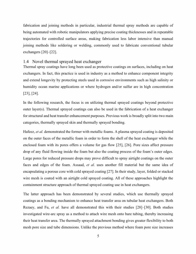
fabrication and joining methods in particular, industrial thermal spray methods are capable of

being automated with robotic manipulators applying precise coating thicknesses and in repeatable

trajectories for controlled surface areas, making fabrication less labor intensive than manual

joining methods like soldering or welding, commonly used to fabricate conventional tubular

exchangers [20]–[22].

1.4 Novel thermal sprayed heat exchanger Thermal spray coatings have long been used as protective coatings on surfaces, including on heat

exchangers. In fact, this practice is used in industry as a method to enhance component integrity

and extend longevity by protecting steels used in corrosive environments such as high salinity or

humidity ocean marine applications or where hydrogen and/or sulfur are in high concentration

[23], [24].

In the following research, the focus is on utilizing thermal sprayed coatings beyond protective

outer layer(s). Thermal sprayed coatings can also be used in the fabrication of a heat exchanger

for structural and heat transfer enhancement purposes. Previous work is broadly split into two main

categories, thermally sprayed skin and thermally sprayed bonding.

Hafeez, et al. demonstrated the former with metallic foams. A plasma sprayed coating is deposited

on the outer faces of the metallic foam in order to form the shell of the heat exchanger while the

enclosed foam with its pores offers a volume for gas flow [25], [26]. Pore sizes affect pressure

drop of any fluid flowing inside the foam but also the coating process of the foam’s outer edges.

Large pores for reduced pressure drops may prove difficult to spray airtight coatings on the outer

faces and edges of the foam. Assaad, et al. uses another fill material but the same idea of

encapsulating a porous core with cold sprayed coating [27]. In their study, layer, folded or stacked

wire mesh is coated with an airtight cold sprayed coating. All of these approaches highlight the

containment structure approach of thermal sprayed coating use in heat exchangers.

The latter approach has been demonstrated by several studies, which use thermally sprayed

coatings as a bonding mechanism to enhance heat transfer area on tubular heat exchangers. Both

Rezaey, and Fu, et al. have all demonstrated this with their studies [28]–[30]. Both studies

investigated wire-arc spray as a method to attach wire mesh onto bare tubing, thereby increasing

their heat transfer area. The thermally sprayed attachment bonding gives greater flexibility to both

mesh pore size and tube dimensions. Unlike the previous method where foam pore size increases

6

greatly disrupts coating feasibility, but small foam pores increase pressure drop, decreasing heat

exchanger efficiency. It is possible to attach mesh with greater variety of pore sizes with thermal

sprayed coating [28]. Thermal sprayed coatings used to bond surface area enhancements onto

substrate, such as fins on tubes, are an alternative to existing bonding methods such as welding or

brazing which may be uneconomical or difficult due to geometry, material properties, or required

application.

1.5 Spray-on-mesh for low grade heat recovery The aforementioned wire-arc coating deposition method is applied to heat exchanger fabrication

such that wire mesh is attached to bare tubing. In doing so, the coating bonds the mesh to the bare

tubes, adding to the heat exchanger heat transfer area and enhancing heat transfer similarly to

welded, brazed or soldered fins in conventional tubular heat exchangers. Because the heat travels

through the tube wall into the coating and from the coating into the mesh (or the reverse direction,

depending on the temperature gradient), the coating must fulfill dual purposes: adequate strength

to hold the mesh in place during operation and high heat transfer coefficient to conduct heat

between the mesh and tube.

In addition, the coating must be able to withstand thermal cycling without cracking or delaminating

as flares may be operated at full capacity only intermittently. The melting point of the heat

exchanger materials must be well in excess of the maximum temperatures that can be reached in

the flare or flue gas stack. The coating must be erosion resistant as there may be particulate matter

carried by the moving gases in the flare or flue stacks. Lastly, coating materials must resist high

temperature corrosion and/or oxidation.

Out of the two aforementioned approaches, the thermally sprayed bonding method is selected over

the thermally sprayed skin due to the low pressure drop and improved fowling resistance. A metal

foam would be difficult to clean once soot and other particulates are trapped within its pores.

Furthermore, a large pressure drop is not feasible in a flare system, especially near the outlet where

flowrates and velocities must be high to facilitate good combustion of VOCs [8]. Wire mesh layers

can be configured to have less pressure drop than foam core.

Previous studies on heat transfer in mesh utilize different heat transfer pathways and predict heat

transfer coefficients or effective conductive coefficients from measurements at the base or edge of

the mesh or stacked mesh network, via soldered or other bonding connection. However the heat

7

transfer enhancement capabilities of a thermally sprayed coating acting as a bonding mechanism

for an extended surface has not been studied in depth at high temperatures and forced convection

flow regime.

The interest in quantifying heat transfer in mesh goes back decades as evident in Tong and

London’s ASME study [31]. In Li and Wirtz’s study, the wire mesh is transferring heat away from

a heated plate which is attached to the mesh base. Heat transfer coefficient is calculated measuring

the rate of heat dissipation. The mesh geometry is a folded serpentine configuration [32]. Chang

introduces a theoretical model to predict an effective thermal conductivity for wire screens which

is highly sensitive to mesh porosity [33]. Shuangtao et al. use ultra-fine fins stacked in many layers

and create a numerical model. The porosity difference between their ultrafine mesh and the mesh

used in the present study is by one or two orders of magnitude [34]. These aforementioned mesh

modeling methods are insufficient for the present study due to differing mesh geometry, mesh heat

transfer application, and mesh connection method.

For a deeper investigation into the flow characteristics in a single mesh wire, Khan, Culham and

Yovanovich model the flow around a mesh to deduce heat transfer coefficients, building upon

basic correlations from Churchill and Bernstein, Morgan, Zukauskas, and Hilpert [35], [36]. The

idea of modeling wire mesh as fins is developed from two separate studies from Tian, et al. and

Wang, et al., both studies use woven meshes whereas the present study investigates welded mesh

[37], [38]. Isothermal fins were modeled in the previous studies, this approach will be enhanced

by addition of adiabatic cross member fins that form the wire mesh.

Tian, et al. use heat transfer from heated face sheets soldered onto mesh layers to quantify heat

transfer coefficient. Their study investigates a host of parameters including wire mesh orientation,

shape, and material [39]. Similarly, Park, Ruch, and Wirtz test multilayered woven and welded

mesh, providing a modified Colburn j-factor [40]. In a study by Jones and Prenger [41], heat is

transferred via a common wall separating two ducts with mesh screens filling the duct cross

section, creating a different heat transfer pathway than the one created in this present study. All

three approaches are similar in terms of heat transfer from base plate onto mesh, and investigate

heat dissipation rates, as such they differ compared to the tube and mesh structure in the present

study. The current study utilizes wire mesh bonded to tube as extended surface enhance forced

8

convection heat transfer performance, imparting more heat into the liquid inside the tubes

ultimately increasing the water inlet and outlet temperature difference.

All aforementioned approaches are slightly different from the present study, whether it is in heat

transfer pathway, mesh type, orientation, geometry, or modeling approach. The closest related

studies were conducted by Fu, et al. and Rezaey in their studies on miniature tubular heat

exchangers with mesh attached via thermal sprayed coating [28]–[30]. The work presented in the

present study provides a more detailed look into wire mesh heat transfer performance

enhancement, coating thermal resistances, and mesh temperature distribution utilizing newly

designed tube and mesh heat exchangers with thermal sprayed coatings.

1.6 Objectives The overall objectives of this study were to develop lab-scale spray-on-mesh and tube heat

exchanger with novel flattened tube profile for improved mesh to tube contact and thermal sprayed

coating application. This can be broken into the following stages:

1. Design and fabricate four lab-scale heat exchanger samples with differing coating parameters to

test the effect on heat exchanger performance.

2. Develop heat transfer model for spray-on mesh to predict outlet temperature with known inlet

properties and predict heat transfer coefficient.

3. Quantify thermal resistances in the thermal sprayed mesh and tube heat exchanger to identify

areas of improvement.

4. Understand fin temperature distribution to provide insight on fin geometry and size in future

designs to improve fin efficiency.

1.7 Thesis organization Thermal sprayed lab-scale tube and mesh heat exchangers were designed and heat transfer

performance was tested. Chapter 2 describes the parametric design decisions as well as fabrication

procedure of lab-scale heat exchangers. Chapter 3 outlines the discretized heat transfer model

proposed to predict outlet water temperature while integrating wire mesh as extended surfaces. A

thermal resistance network is developed in order to compare the thermal resistances throughout

the heat exchanger heat transfer network. Chapter 4 discusses the experimental methods using the

custom designed heated duct setup for the forced convection heat transfer tests. Chapter 5 presents

9

the results and discussion. Measured temperature differences are presented as results of the heated

air force convection tests. Included in this section are resulting thermal sprayed coating cross

sections deposited with the various spray parameter combinations. Chapter 6 details conclusion

and possible future work for consideration.

10

2 Lab-scale meshed tubular heat exchanger design and

fabrication

2.1 Design of lab-scale heat exchangers

2.1.1 Tubing machining method The flat tube design of the miniature heat exchangers is a continuation of the work completed by

Rezaey and Fu, et al. with additional learnings being applied from attempts at testing Rezaey’s

industrial scale prototype heat exchanger [28]–[30]. Details on the attempted tests and difficulties

encountered with regards to the prototype heat exchanger are detailed in the Appendix A.

Fu, et al. used U shaped bends due to the ductile nature of aluminum [30]. Rezaey used threaded

pipe elbow joints to form the U shape bends due to less ductile stainless-steel tubing selected as

material for their miniature heat exchangers [28]. It was noted that the joint fittings were prone to

leakage. Considering usage cases where the heat exchanger is at -40 degrees Celsius winter

ambient outdoor temperature initially, and heated up to several hundred degrees when the flare or

flue gas exhaust is operating, thermal expansion and contraction could cause leakage in threaded

elbows which connect the heat exchanger tubing. Eliminating any extra leak points is beneficial to

operational reliability.

Images of both prior designs are shown in the figure below. In both designs, a woven wire mesh

is either placed flat atop of the tube or bent around the tubing in a wavy pattern to maximize

conformity to the tubing surfaces.

Figure 3: Rezaey (Left) and Fu (Right) lab scale samples [28], [30]

11

The design chosen going forward adopts elements of both previous designs. A thicker wall

stainless steel tube is used. This tube can be bent, thus eliminating costs and leakage associated

with the elbow fittings while increasing the operating temperature with a higher melting point

material compared to aluminum. An additional design change is introduced. The rectangular area

where the wire mesh is to be joined to the tube will be compressed flat. The flattening of tubes was

derived from a study on flattened tube external flows for improved efficiency in residential heat

pump systems [42]. Although the study focuses on flattened tubes oriented parallel to the airflow

to decrease pressure losses, the flattened tube profile served as inspiration for the design in the

present study. The study does not utilize surface area enhancements such as mesh attached via

thermal spray. A diagram of the flattened tube cross section is included below. It is assumed that

the tube outer perimeter does not change and the tube flattening process does not affect the

thickness of the tubing.

Figure 4: Tube dimensions round (Left) and flattened (Right)

Wire mesh acts as an extended surface attached to the bare, flattened tube. It was hypothesized

that a flattened tube surface will provide a better mating surface between the flat wire mesh and

the tube surface increasing both strength of the bond between the mesh to tube as well as heat

transfer performance by decreasing thermal resistance with increasing contact surface area. This

assembly method also eliminates the wavy pattern previously required for adhering mesh to tube,

improving manufacturability. Flattening the tube is a one step process and is less complex than

bending the flat mesh around round tubing and ensuring the mesh is in contact with the tube at all

points. A drawing of the assembly and press fabricated for compressing the tubing is included in

the Appendix B. A bent and flattened bare tube sample is pictured below.

12

Figure 5: Bent and flattened bare tube heat exchanger

All design choices included consideration for machinability and compatibility with existing off-

the-shelf components. The tubing was available as standard 9.53 mm (3/8-inch) outer diameter,

fitting standard sized tube benders. The flattening press was cut with waterjet from steel plate.

Compression force is achieved by using high strength nuts and bolts inserted into bolt holes

throughout the steel plate, by design. The tubing ends were also left non-flattened to fit onto

industry standard compression fittings. This allows for direct integration with standardized pipe

fittings such as NPT threaded hydraulic appurtenances.

2.1.2 Wire mesh selection There are many types of wire mesh available from off-the-shelf suppliers. Mesh comes in two

construction methods: weaved and welded. The convenience of off-the-shelf mesh offers includes

variety in pore sizes and wire diameter. Instead of the previously used weaved wire mesh, a welded

mesh is selected. In weaved mesh, the wires used in the mesh are interlaced creating a woven

texture which is not flat. Wires are interlocked above and below each other so they are no longer

straight, nor is the mesh truly flat. In welded mesh, the wire above, always stays on top and the

wire below always stays at the bottom. Thus, creating a much flatter mesh, suitable for bonding

onto bare tubing. Woven mesh also has steel wires in contact but not attached, whereas in welded

13

mesh, the wires are fused together decreasing contact resistance for heat transfer between mesh

wires.

Figure 6: Welded mesh sample [43]

Figure 7: Woven mesh sample [44]

The welded 4 pores per inch (PPI) mesh was selected due to previous experiments showing that

despite mesh density increasing (pore sizes decreasing) pressure drop across the samples were

quite low for meshes with pore sizes between 0.1 to 0.5 inches. Furthermore, smaller pore sizes up

to 10 PPI increase heat transfer performance, it was only at 20 PPI, that temperature differences

began to decrease [28]. The denser mesh has thinner wire which further improves machinability.

During fabrication, the wire mesh sheets were easily cut using a sheet metal brake because the

wire diameter was in the same as the sheet metal thickness the brake was designed to cut. Welded

mesh also holds its shape well without fraying after cutting or slight bending. Woven mesh wires

at the edges of a mesh patch tend to fray and fall out during handling.

2.1.3 Mesh clamping method The wire mesh clamping method was finalized through many iterative tests. Initially, small

diameter metal wire was used to tie mesh to tube every few inches along the tube. This works well

to create small test pieces but was very time consuming as wire had to be bent, cut, and twisted

tightly to ensure a close bond between the wire mesh sheet and the bare tube’s flattened face. Wires

14

used to tie the mesh to tube were not removable after the sample was coated as they were coated

along with the wire mesh.

Securing two layers of mesh sheet, sandwiching the tube, was difficult with the wire tie method.

Wires would not easily feed through wire mesh pores and line up while wrapping around the tube.

Another method was tested with machine screws and nuts. Screw heads and nuts were large enough

to interfere with the wire mesh pores, screw shank and thread sections could fit through the mesh.

This method was much quicker than using wires to tie the mesh(es) to the tube. Every few inches,

a screw and nut were used to compress the two sheets of mesh against the tube. Furthermore, this

method allowed most of the screws to be removed after spraying so long as their threads were not

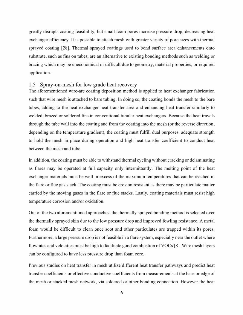
filled with coating, jamming the nut permanently. The following figure shows both wire mesh

clamping methods.

Figure 8: Two wire mesh clamping methods, wire tie method (L) compared with screw and nut method (R) with partial masking

by aluminum foil to protect screw threads from coating deposition

During the wire-arc spraying process, samples were masked such that the only exposed areas were

where mesh was over bare tube. This selective deposition would ensure as much bare mesh was

left on the sample as possible because coated mesh would decrease heat transfer performance

compared to bare mesh. The coating was only to be used to attached mesh to tube. The masking

15

also protected the threads of the machine screws from being filled with coating so the nuts could

be unscrewed after the coating process was complete. Several masking methods were trialed

utilizing woven heat resistant tapes, aluminum foil and finally aluminum sheet in order to mask

the coating without melting onto the mesh and bonding to the sample. Masking was also required

on the tube ends to ensure they were smooth and intact for installation of compression fittings at a

later stage of the experiment.

Figure 9: Various sample masking tests, heat resistant tape (Top Left), tape melted onto mesh after spraying (Top Right),

Aluminum foil over tap (Bottom Left), and Aluminum sheet secured with wire (Bottom Right)

Securing the sample in the sample holder placed within the spray hood was also an iterative

process. Initially, samples were placed onto a vertical plate and clamped at one end with clamps

placed on the bare tube section of the sample. This method was unfeasible as the samples moved

during the spray process due to the air pressure and particles launched from the torch nozzle onto

the sample. Both ends were clamped for the next test. The clamping method was deemed

unfeasible because the clamping force required to hold the samples securely meant that the screws

securing the mesh were compressed against the sample holder backplate and causing the mesh to

be pushed away from the tube surface. In the end, for the single pass linear pattern sample, a

modified clamping method was used to clamp the masking material rather than the tube or mesh.

16

For the rectangular spray pattern samples (see next section for explanation on spray patterns), a

thin wire was used to hang the sample from a different sample holder setup to avoid putting

pressure on the sample and causing gaps between mesh and tube while ensuring the sample stayed

in place during spraying. The full-sized samples were much heavier than the test pieces so

movement during thermal spray deposition was not a concern. The final configuration for the mesh

on tube heat exchanger samples is shown in the figure below.

Figure 10: Heat exchanger tube with wire mesh fastened by screws and nuts, masked with aluminum sheet, hung from sample

holder with wire, tube ends protected with masking tape

2.2 Experimental Method

2.2.1 Wire-arc spray fabrication A high-density arc spray coating system (Thermion AVD 456 HD, Thermion Inc. WA, USA) was

used to spray stainless steel wire (Metcoloy 2, Oerlikon Surface Solutions AG, ZH, Switzerland)

onto the flattened tube and mesh sheet assemblies. Four samples are fabricated in order to compare

several coating parameters. In this study, there are two aspects of the coating process which are

manipulated, spray nozzle tip trajectory and speed. All other spray parameters were set in

accordance to the results of a previous study which found the appropriate standoff distance, current

and voltages to deposit the strongest and least porous coating [29]. A custom gantry style robotic

manipulator was set to two torch tip movement speeds: 500 and 1000 inches per minute.

17

Two spray patterns were utilized. For the rectangular pattern, the robot sprays one horizontal pass

followed by a small vertical step and then another horizontal pass in the opposite direction

followed by a small vertical step, continuing for a user specified total vertical distance and

horizontal pass length, forming a rectangular spray area. A linear pattern was also possible due to

the slender coated area where the mesh is over the flattened tube section and the sufficient width

of the wire-arc spray plume. Only the interface area where the mesh is in contact with the tube flat

surface requires coating deposition in order to bond the mesh to the tube. A single pass back and

forth over the mesh where the tube is located creates a more consistent coating with the plume

centered directly over the area of interest. See the figure below for a schematic of the different

spray patterns on the lab scale heat exchanger sample. The following table summarizes the spray

parameters used in the fabrication of lab scale spray-on mesh heat exchangers.

Figure 11: Rectangular shape spray torch trajectory (Left) and linear torch trajectory (Right)

Table 1: Wire arc spray parameters (settings for best coating as defined in previous work [29])

Parameter Value

Torch Value Arc

Wire feed rate 7 m/min

Voltage 34 V

Inlet Pressure 689 kPa (100 psi)

Standoff distance 152.4 mm (6 inches)

Coating thickness was determined based on mesh wire diameter. The wire used had a 0.81 mm

(0.032-inch) diameter. Actual sample thicknesses are not possible to measure because the coating

does not spray evenly onto the wire mesh and tube interface resulting in areas of thinner coating

18

atop the wires and thicker coating where wire mesh pores topology accumulated thermal sprayed

coating. Several small test pieces of mesh and tube were used to test different coating thicknesses

before any samples of the lab scale heat exchangers were made. A few passes were deposited each

time, after which the sample thickness and weight were measured. It was determined through cross

section cuts put under a microscope, coatings greater than 0.9 mm thickness was sufficient in fully

embedding the wire underneath the coating and onto the flattened tube surface. Bare tube segments

were used to test the coating thickness buildup per pass. This information was used to fabricate

the meshed samples. It was found that for the 212 mm/s low spray torch tip speed (500 in/min),

11 passes were sufficient to build up a 0.9 mm thick coating. For the 423 mm/s high-speed spray

(1000 in/min), 22 passes were required.

19

3 Mathematical model for lab-scale heat exchanger heat

transfer heat transfer analysis

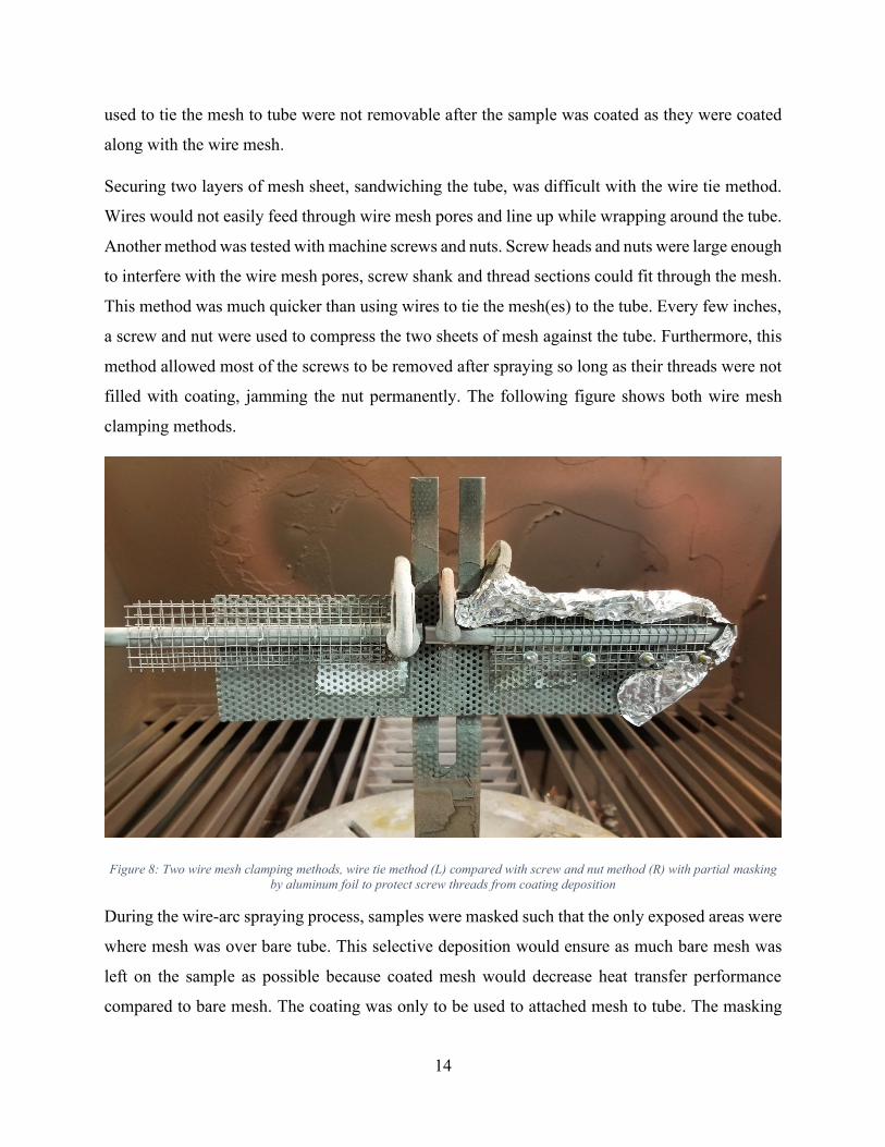
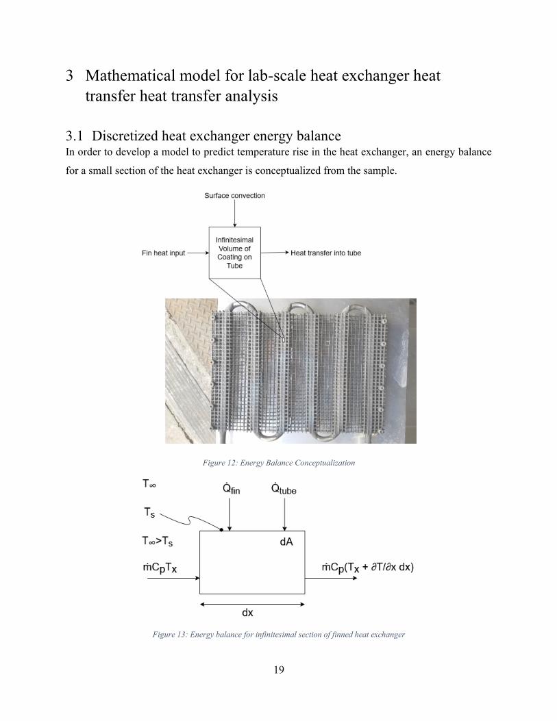
3.1 Discretized heat exchanger energy balance In order to develop a model to predict temperature rise in the heat exchanger, an energy balance

for a small section of the heat exchanger is conceptualized from the sample.

Figure 12: Energy Balance Conceptualization

Figure 13: Energy balance for infinitesimal section of finned heat exchanger

20

From this energy balance, we can derive a first order different equation as follows:

�̇�𝐶p𝑇 + �̇�fin + �̇�tube = �̇�𝐶p (𝑇 +𝜕𝑇

𝜕𝑥𝑑𝑥) (3 − 1)

�̇�𝐶p𝑇 + �̇�fin𝑑𝑥 + 𝑈tube𝑑𝐴tube(𝑇∞ − 𝑇s) = �̇�𝐶p (𝑇 +𝜕𝑇

𝜕𝑥𝑑𝑥) (3 − 2)

If wall resistance is neglected, assuming perfect contact between fin and tube 𝑇s =

𝑇water inside = 𝑇, furthermore 𝑑𝐴tube = 𝑃tube𝑑𝑥, then the equation simplifies to:

�̇�fin + 𝑈tube𝑃tube(𝑇∞ − 𝑇) = �̇�𝐶𝑝

𝜕𝑇

𝜕𝑥(3 − 3)

𝑑𝑇

𝑑𝑥+

𝑈tube𝑃tube

�̇�𝐶p𝑇 =

𝑈tube𝑃tube

�̇�𝐶p𝑇∞ + �̇�fin (3 − 4)

3.2 Defining all components of �̇�fin for each discretized segment In order to quantify the contribution of the mesh wires, they are modelled as fins. The wire spacing

in the fin creates pores in the mesh that are 6.35 by 6.35 mm (0.25 by 0.25 inch). Thus, it is

convenient to consider each unit cell consisting of a single wire (with cross wires) and divide the

heat exchanger into 6.35 mm (0.25-inch) sections. �̇�fin is a constant for each segment (𝑑𝑥 =

6.35 mm) and is composed of two types of wires modelled as two types of fins. Longitudinal wires

are bonded directly to the tube with thermal sprayed coating. The grey rectangle in the above

diagram represents the thermal spray coating adhering the wire mesh to the tube. Longitudinal

wires extend outwards from the tube axially. Connected to longitudinal wires are transverse wires

which extend perpendicularly, at regular intervals, from the longitudinal wires.

Figure 14: Unit cell section of heat exchanger (L) and three consecutive H-EX segments with different colored fins (R)

21

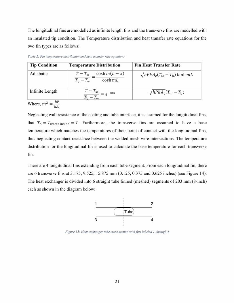
The longitudinal fins are modelled as infinite length fins and the transverse fins are modelled with

an insulated tip condition. The Temperature distribution and heat transfer rate equations for the

two fin types are as follows:

Table 2: Fin temperature distribution and heat transfer rate equations

Tip Condition Temperature Distribution Fin Heat Transfer Rate

Adiabatic 𝑇 − 𝑇∞

𝑇b − 𝑇∞=

cosh 𝑚(𝐿 − 𝑥)

cosh 𝑚𝐿

√ℎ𝑃𝑘𝐴c(𝑇∞ − 𝑇b) tanh 𝑚𝐿

Infinite Length 𝑇 − 𝑇∞

𝑇b − 𝑇∞= 𝑒−𝑚𝑥 √ℎ𝑃𝑘𝐴c(𝑇∞ − 𝑇b)

Where, 𝑚2 =ℎ𝑃

𝑘𝐴c

Neglecting wall resistance of the coating and tube interface, it is assumed for the longitudinal fins,

that 𝑇b = 𝑇water inside = 𝑇. Furthermore, the transverse fins are assumed to have a base

temperature which matches the temperatures of their point of contact with the longitudinal fins,

thus neglecting contact resistance between the welded mesh wire intersections. The temperature

distribution for the longitudinal fin is used to calculate the base temperature for each transverse

fin.

There are 4 longitudinal fins extending from each tube segment. From each longitudinal fin, there

are 6 transverse fins at 3.175, 9.525, 15.875 mm (0.125, 0.375 and 0.625 inches) (see Figure 14).

The heat exchanger is divided into 6 straight tube finned (meshed) segments of 203 mm (8-inch)

each as shown in the diagram below:

Figure 15: Heat exchanger tube cross section with fins labeled 1 through 4

22

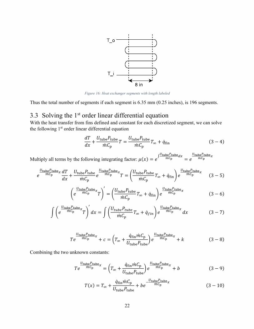
Figure 16: Heat exchanger segments with length labeled

Thus the total number of segments if each segment is 6.35 mm (0.25 inches), is 196 segments.

3.3 Solving the 1st order linear differential equation With the heat transfer from fins defined and constant for each discretized segment, we can solve

the following 1st order linear differential equation

𝑑𝑇

𝑑𝑥+

𝑈tube𝑃tube

�̇�𝐶p𝑇 =

𝑈tube𝑃tube

�̇�𝐶p𝑇∞ + �̇�fin (3 − 4)

Multiply all terms by the following integrating factor: 𝜇(𝑥) = 𝑒∫

𝑈tube𝑃tube�̇�𝐶p

𝑑𝑥= 𝑒


𝑥

𝑒𝑈tube𝑃tube

�̇�𝐶p𝑥 𝑑𝑇

𝑑𝑥+

𝑈tube𝑃tube

�̇�𝐶p𝑒


𝑥𝑇 = (

𝑈tube𝑃tube

�̇�𝐶p𝑇∞ + �̇�fin) 𝑒


𝑥(3 − 5)

(𝑒𝑈tube𝑃tube

�̇�𝐶p𝑥

𝑇)

′

= (𝑈tube𝑃tube

�̇�𝐶p𝑇∞ + �̇�fin) 𝑒


𝑥(3 − 6)

∫ (𝑒𝑈tube𝑃tube

�̇�𝐶p𝑥

𝑇)

′

𝑑𝑥 = ∫ (𝑈𝑡𝑢𝑏𝑒𝑃𝑡𝑢𝑏𝑒

�̇�𝐶𝑝𝑇∞ + �̇�𝑓𝑖𝑛) 𝑒


𝑥𝑑𝑥 (3 − 7)

𝑇𝑒𝑈tube𝑃tube

�̇�𝐶p𝑥

+ 𝑐 = (𝑇∞ +�̇�fin�̇�𝐶p

𝑈tube𝑃tube) 𝑒


𝑥+ 𝑘 (3 − 8)

Combining the two unknown constants:

𝑇𝑒𝑈tube𝑃tube

�̇�𝐶p𝑥

= (𝑇∞ +�̇�fin�̇�𝐶p



𝑥+ 𝑏 (3 − 9)

𝑇(𝑥) = 𝑇∞ +�̇�fin�̇�𝐶p

𝑈tube𝑃tube+ 𝑏𝑒

−𝑈tube𝑃tube

�̇�𝐶p𝑥

(3 − 10)

23

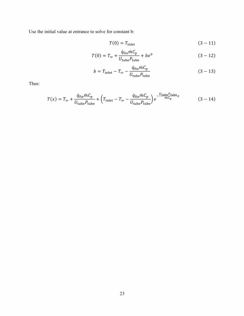
Use the initial value at entrance to solve for constant b:

𝑇(0) = 𝑇inlet (3 − 11)

𝑇(0) = 𝑇∞ +�̇�fin�̇�𝐶p

𝑈tube𝑃tube+ 𝑏𝑒0 (3 − 12)

𝑏 = 𝑇inlet − 𝑇∞ −�̇�fin�̇�𝐶p

𝑈tube𝑃tube

(3 − 13)

Thus:

𝑇(𝑥) = 𝑇∞ +�̇�fin�̇�𝐶p

𝑈tube𝑃tube+ (𝑇inlet − 𝑇∞ −

�̇�fin�̇�𝐶p


−𝑈tube𝑃tube

�̇�𝐶p𝑥

(3 − 14)

24

4 Application of lab-scale heat exchangers in heated air tests

4.1 Design of simple heated wind tunnel

4.1.1 Fan and duct design In order to test the heat exchanger in conditions similar to flare stack exhausts, a testing apparatus

consisting of a fan and duct were designed. Previous learnings from the three prototype heat

exchanger tests show that the following factors are guidelines in the design in order to achieve a

measurable inlet to outlet temperature difference:

• A high temperature air source is required, on the order of several hundred degrees Celsius

• Air source must also flow quickly in the order of several meters per second for convection

• The quick flowing air must be hot enough or the duct insulated enough so the air is still hot upon

reaching the heat exchanger tube / mesh

• The duct length must be sufficient to allow air to mix to a uniform temperature after being heated

and before reaching the heat exchangers located downstream inside the duct

• The difference in crossflow air and tube water temperature should be maximized

• The heat source should not be a point source or moved across the heat exchanger cross section

• A distributed heat source is ideal, the heat exchanger samples should occupy the whole duct cross

section in order to capture maximum heat

A previous duct and fan combo unit utilized a vane axial fan (DDA12T10033B, Canarm/LFI Ltd.

ON, Canada) to propel air into a rectangular cross section duct. The setup was effective at moving

air upwards of 5 m/s, as such another fan was ordered in-kind from Canarm Ltd. A custom duct

with integrated adapter was designed and sent to Midwest Fabricators Ltd. Drawings for the duct

are shown in below. One end of the duct is designed to fit the 1-foot diameter axial fan outlet. The

duct transitions into a 254 mm by 305 mm (10 inch by 12 inch) rectangle cross-section in order to

fit the lab scale heat exchangers, the photograph in the figure shows the fit.

25

Figure 17: Duct drawing and detailed views of slot, sample fitment, and torch insertion

4.1.2 Heating source for duct A propane torch setup was utilized in order to provide sufficient heat input into the air flowing

inside the duct in order to heat the air upwards of 700 degrees Celsius. Preliminary testing of this

heating method was conducted with an existing galvanized sheet metal duct and fan system which

26

was built for cold room testing. The propane torch design was inspired by propane fed, forced air

construction site heaters. Upon verifying the proposed heating method was sufficient at achieving

the high temperature airflow, a stainless-steel duct was built in order to withstand the extreme heat

and flame impingement as the thin galvanized duct warped from the high temperatures.

A hole was cut in the side of the stainless-steel duct, slightly downstream from the vane axial fan,

in order to feed the torch tip into the duct. The propane torch (Model No. 95-B, Tiger Torch Ltd.

AB, Canada), fan and duct setup was constructed at the University of Alberta Protective Clothing

and Equipment Research Facility. This lab designed for combustion testing in order to ensure safe

operation. A custom electrical trigger and igniter box was wired to ensure controlled ignition and

safe operation. Extra foil tape was used to seal the area around the torch tip to prevent airflow

escaping and drawing the flame out at the port in the duct instead of downstream of the duct.

A regulator was used on the propane tank, the outlet pressure was set at 34 kPa (5 psi), the lowest

level required for consistent ignition and stable combustion. Custom sized orifices were inserted

into the torch stem to further adjust the gas flow in order to have stable combustion while the fan

was blowing over the torch tip inside of the duct. At higher gas regulator settings, the flame tips

could extend outside of the duct (several feet in length) and create extremely high temperatures

(measured upwards of 700 degrees Celsius). The final pressure was set such that there was

sufficient combustion gas pressure at the torch tip such that the flame stayed ignited near the torch

tip and did not burn back up the torch stem. In an effort to protect and preserve the samples during

initial testing, for the following tests the pressure was decreases such that the flame length was

contained within the duct and not directly impinging onto the samples. As such, future tests which

aim to push the upper limits of the materials can be conducted at higher pressures.

Figure 18: Propane torch flames reaching the outlet of the duct (Left), Propane torch head sealed into duct port with heat

resistant foil tape (Right)

27

4.2 Experimental method Samples were placed near the outlet of the duct where a set of movable covers were installed. The

covers were guided by rails near the outlet of the duct to allow the sample to move forward and

backwards up to 457 mm (18 inches) (see Figure 17). Samples were placed as far back as the duct

opening allowed and the flame was extended as far downstream as possible (by adjusting the

regulator pressure) to heat the air up as much as possible but without directly impinging onto the

samples themselves. Thus the samples were considered to be heated by flame heated air only.

4.2.1 Fan and propane torch operation The fan was started and sufficient time elapsed to ensure the fan was spinning at full speed before

the torch was ignited. Because of the placement of the torch directly downstream of the fan, it was

imperative that the torch was ignited only after the fan was operating. Otherwise, without the

airflow, the flame would cause damage to the fan and duct area closest to the torch tip. Each test

could require upwards of ten minutes to reach steady state, care is required to ensure propane

pressure is constant throughout the test and fan temperatures are not too high to damage the motor.

Operating the propane torch heated duct and fan system for more than fifteen minutes continuously

resulted in the fan noise changing and suspected degradation of performance. As such, operating

the system for longer than required is not recommended unless a higher temperature rated fan or

fan cooling system is used.

4.2.2 Hydraulic system configuration Domestic cold water was supplied through a hose, into a fine particulate filter and throttling glove

valve before being fed through a turbine flow meter (FTB-421, Omega Engineering, Inc. QC,

Canada) just upstream of the sample, and finally into the lab scale heat exchanger samples. The

turbine flow meter was connected to a Teensy USB Development Board (3.2, PJRC.COM, LLC.

OR, USA) with a frequency counter program loaded into the board, as USB cable attached to a

laptop computer displays the readout.

Lab scale heat exchangers were made from 9.5 mm (3/8-inch) diameter stainless steel tubing (SS-

T6-S-035-6M, Swagelok Company, OH,USA) bent to shape and flattened at specific lengths. At

each inlet and outlet of the samples, a threaded compression fitting (SS-600-1-4, Swagelok

Company, OH,USA) connected to a tee fitting (SS-4-T, Swagelok Company, OH,USA) is used to

allow for a probe tip J-type thermocouple (TC-J-NPT-G-72, Omega Engineering, Inc. QC,

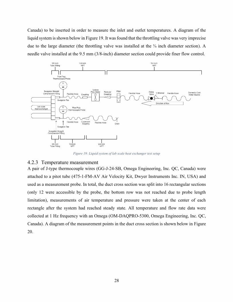
28

Canada) to be inserted in order to measure the inlet and outlet temperatures. A diagram of the

liquid system is shown below in Figure 19. It was found that the throttling valve was very imprecise

due to the large diameter (the throttling valve was installed at the ¾ inch diameter section). A

needle valve installed at the 9.5 mm (3/8-inch) diameter section could provide finer flow control.

Figure 19: Liquid system of lab scale heat exchanger test setup

4.2.3 Temperature measurement A pair of J-type thermocouple wires (GG-J-24-SB, Omega Engineering, Inc. QC, Canada) were

attached to a pitot tube (475-1-FM-AV Air Velocity Kit, Dwyer Instruments Inc. IN, USA) and

used as a measurement probe. In total, the duct cross section was split into 16 rectangular sections

(only 12 were accessible by the probe, the bottom row was not reached due to probe length

limitation), measurements of air temperature and pressure were taken at the center of each

rectangle after the system had reached steady state. All temperature and flow rate data were

collected at 1 Hz frequency with an Omega (OM-DAQPRO-5300, Omega Engineering, Inc. QC,

Canada). A diagram of the measurement points in the duct cross section is shown below in Figure

20.

29

Figure 20: Duct cross section measurement points (red dots) for air pressure and temperature, Pitot tube and thermocouple

probe used for measurements (Bottom Left)

Five heat exchanger samples were tested inside the heated duct. One sample was a bent and

flattened bare tube, with the four other samples each made with a different coating application

trajectory and thickness combination. Each sample was tested at four water flow rates: 560, 860,

1120, and 1400 mL/minute. Airflow was supplied by a constant single speed fan and air speed

varied based on sample porosity. To ensure measurements were recorded at steady state, the test

was stopped only when the measured outlet water temperature no longer increased for at least 45

seconds.

30

5 Results and Discussion

5.1 Steady state measurements

5.1.1 Water temperature difference at four flowrate set points Steady state water temperature difference measurements for each of the five samples are presented

in the table below. Each sample is tested at four flowrates: 560, 860, 1120, and 1400 mL/min. Inlet

temperatures are a measurement of the domestic cold-water supply temperature which fluctuated

between 8 to 12 degrees Celsius. A previous study by Rezaey tested similar samples of reduced

size (7 inch by 7 inch vs. 12 inch by 8 inch) and tube diameter (1/4 inch outer diameter vs. 3/8

inch outer diameter) at flowrates from 500 to 900 mL/min [28]. The lower two flow rates tested in

the present study can be used as comparisons to the previous study.

Table 3: Inlet and outlet water temperature measurements for each sample at four flowrates

Sample Flowrate Tinlet Toutlet ∆T

- mL/min ℃ ℃ ℃

Bare Tube 560 11.2 25.8 14.6

Bare Tube 860 9.6 19.9 10.3

Bare Tube 1120 9.4 18.0 8.6

Bare Tube 1400 12.2 17.1 4.9

500 in/min, Rectangular Pattern, Thin 560 11.2 29.9 18.7








500 in/min, Rectangular Pattern, Thick 560 7.7 51.4 43.7




500 in/min, Linear Pattern, Medium 560 9.4 38.5 29.1




5.1.2 Air temperature measurements In the table below, the average air temperature and speeds for each sample is listed. As expected,

the bare tube sample, which had the least airflow restrictions, resulted in the highest air speed. Air

speed and air temperature have an inverse relationship. When the axial fan supplied airflow is

31

unrestricted, the air carries the heat from the propane torch flame out of the duct at a more rapid

rate and therefore lowers the duct average air temperature. Hence, for the bare tube sample, average

duct air temperature measured at the sample is lowest. For the thickest coated sample, the reduction

in mesh porosity caused by the thicker coating results in airflow restrictions. This is evident in the

lowest measured average air speed. Air accumulating upstream of the sample reduces the rate that

the air carries the heat out of the duct, therefore increasing the air temperature measured at the

sample.

Table 4: Crossflow air temperature and speed measurement

Sample Average Air Temp Average Speed

- ℃ m/s

Bare Tube 177 ± 126 (n = 12) 8.4 ± 2.9 (n = 12)

500 in/min, Linear Pattern, Medium Coating 223 ± 184 (n = 12) 6.4 ± 3.9 (n = 12)

1000 in/min, Rectangular Pattern, Thin Coating 237 ± 201 (n = 12) 5.8 ± 3.4 (n = 12)

500 in/min, Rectangular Pattern, Thin Coating 227 ± 187 (n = 12) 5.8 ± 3.5 (n = 12)

500 in/min, Rectangular Pattern, Thick Coating 272 ± 187 (n = 12) 4.8 ± 1.0 (n = 12)

There is a large standard deviation for both air temperature and speed. A mesh section upstream

of the sample could be used in the duct to promote better mixing of the air for a more uniform

temperature. A flow straightener could also be used to decrease the lateral velocities of the air to

reduce speed (pressure) measurement differences. Increased number of measurements may also

help to reduce standard deviation and identify measurement outliers after normal distribution is

demonstrated.

The figure below is a plot of the temperature difference data for each flowrate across all five

samples. As expected, the coating thickness has a direct relation to temperature difference. Thicker

coated samples had greater water inlet and outlet temperature difference. Bare tube samples had

the smallest temperature difference, meaning all meshed samples exhibited heat transfer

enhancements from the wire mesh extended surface. Lower flow rates resulted in higher water

inlet and outlet temperature differences because the water had a longer duration spent inside the

heated area of the heat exchanger and was subjected to higher amounts of heat transferred into the

same volume than at higher flow rates.

32

Figure 21: Temperature difference plot for all samples at four flow rates

In general, the temperature difference treads agree with the previous study by Rezaey. The

magnitude of temperature difference however, was 1.5 to 4 times greater than measured from

Rezaey’s studies [28]. This increased performance is due to several factors which differentiate the

samples in the present study from the previous study. Factors which serve to enhance the

performance of the samples in the present study compared to Rezaey’s study include larger mesh

area, longer heated tube length, and thicker coating between wire mesh and tube. Factors which

benefit Rezaey’s samples in terms of heat transfer performance include higher pore density mesh

(5, 10, 20 PPI vs. 4 PPI in the present study), higher average air temperatures (upwards of 320

degrees Celsius vs. 272 degrees Celsius), thinner tube wall (0.01 inch vs. 0.035 inch), and smaller

diameter tubing (1/4 inch vs. 3/8 inch). Despite more factors leaning in favor of samples in

Rezaey’s study, the results are indicative that coating thickness between the mesh and tube greatly

improve the heat transfer performance over the other factors. Coating thickness thermal resistances

are further discussed and quantified in section 5.6.

0

5

10

15

20

25

30

35

40

45

50

400 600 800 1000 1200 1400 1600

Tem

per

atu

re D

iffe

ren

ce (

Cel

siu

s)

Flowrate (mL/min)

500 in/min, Rectangular Pattern,Thick Coating

500 in/min, Linear Pattern, MediumCoating

500 in/min, Rectangular Pattern, ThinCoating

1000 in/min, Rectangular Pattern,Thin Coating

Bare Tube

33

5.2 Flow characterization in lab-scale heat exchangers

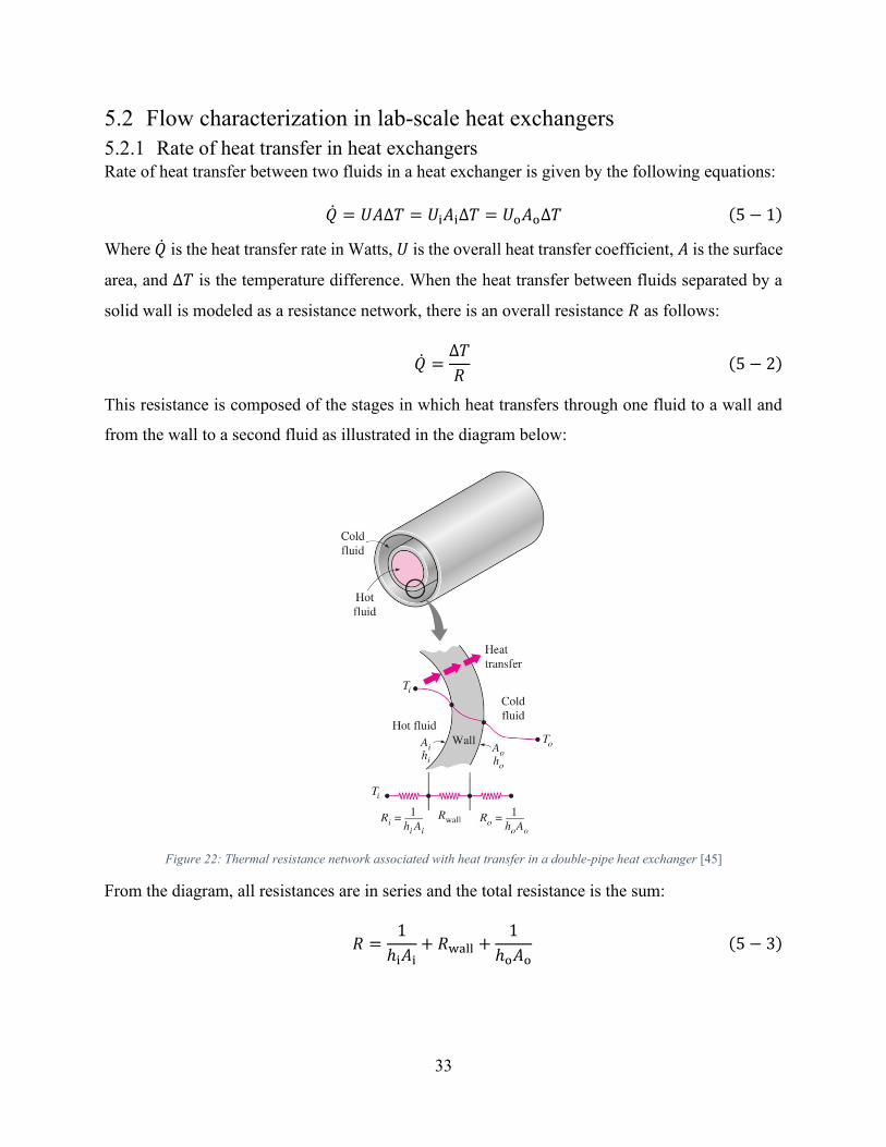
5.2.1 Rate of heat transfer in heat exchangers Rate of heat transfer between two fluids in a heat exchanger is given by the following equations:

�̇� = 𝑈𝐴∆𝑇 = 𝑈i𝐴i∆𝑇 = 𝑈o𝐴o∆𝑇 (5 − 1)

Where �̇� is the heat transfer rate in Watts, 𝑈 is the overall heat transfer coefficient, 𝐴 is the surface

area, and ∆𝑇 is the temperature difference. When the heat transfer between fluids separated by a

solid wall is modeled as a resistance network, there is an overall resistance 𝑅 as follows:

�̇� =∆𝑇

𝑅(5 − 2)

This resistance is composed of the stages in which heat transfers through one fluid to a wall and

from the wall to a second fluid as illustrated in the diagram below:

Figure 22: Thermal resistance network associated with heat transfer in a double-pipe heat exchanger [45]

From the diagram, all resistances are in series and the total resistance is the sum:

𝑅 =1

ℎi𝐴i+ 𝑅wall +

1

ℎo𝐴o

(5 − 3)

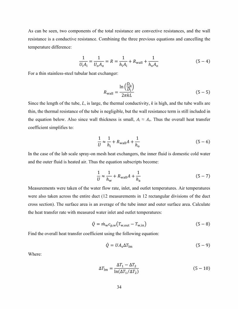
34

As can be seen, two components of the total resistance are convective resistances, and the wall

resistance is a conductive resistance. Combining the three previous equations and cancelling the

temperature difference:

1

𝑈i𝐴i=

1

𝑈o𝐴o= 𝑅 =

1

ℎi𝐴i+ 𝑅wall +

1

ℎo𝐴o

(5 − 4)

For a thin stainless-steel tubular heat exchanger:

𝑅wall =ln (

𝐷o

𝐷i)

2𝜋𝑘𝐿(5 − 5)

Since the length of the tube, L, is large, the thermal conductivity, k is high, and the tube walls are

thin, the thermal resistance of the tube is negligible, but the wall resistance term is still included in

the equation below. Also since wall thickness is small, Ai ≈ Ao. Thus the overall heat transfer

coefficient simplifies to:

1

𝑈≈

1

ℎi+ 𝑅wall𝐴 +

1

ℎo

(5 − 6)

In the case of the lab scale spray-on mesh heat exchangers, the inner fluid is domestic cold water

and the outer fluid is heated air. Thus the equation subscripts become:

1

𝑈≈

1

ℎw+ 𝑅wall𝐴 +

1

ℎa

(5 − 7)

Measurements were taken of the water flow rate, inlet, and outlet temperatures. Air temperatures

were also taken across the entire duct (12 measurements in 12 rectangular divisions of the duct

cross section). The surface area is an average of the tube inner and outer surface area. Calculate

the heat transfer rate with measured water inlet and outlet temperatures:

�̇� = �̇�w𝑐p,w(𝑇w,out − 𝑇w,in) (5 − 8)

Find the overall heat transfer coefficient using the following equation:

�̇� = 𝑈𝐴s∆𝑇lm (5 − 9)

Where:

∆𝑇lm =∆𝑇1 − ∆𝑇2

ln(∆𝑇1 ∆𝑇2⁄ )(5 − 10)

35

Thus the overall heat transfer can be calculated as follows:

𝑈 =�̇�w𝑐p,w(𝑇w,out − 𝑇w,in)

𝐴s∆𝑇lm

(5 − 11)

5.2.2 Internal flow heat transfer coefficient Using well established internal flow characteristics, we can find hw via Nusselt number

correlations) and subtract it from the overall heat transfer to ultimately find ha:

ℎa = (1

𝑈−

1

ℎw− 𝑅wall𝐴)

−1

(5 − 12)

The bare tube samples were tested at four different water flow rates. For the two lower flow rates,

the flow is laminar and a Nusselt number can be found in tables such as the following, provided in

Cengel’s textbook:

Figure 23: Table of Nusselt numbers for various tube cross sections [45]

For the two higher flow rates, the flow is turbulent and the Nusselt number can be found with the

Gnielinski equation, valid for developing or fully developed turbulent flow in smooth tubes:

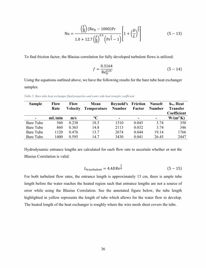
36

Nu =(

𝑓8

) (ReD − 1000)Pr

1.0 + 12.7 (𝑓8

)0.5

(Pr23 − 1)

[1 + (𝐷

𝐿)

23

] (5 − 13)

To find friction factor, the Blasius correlation for fully developed turbulent flows is utilized:

𝑓 =0.3164

ReD0.25

(5 − 14)

Using the equations outlined above, we have the following results for the bare tube heat exchanger

samples:

Table 5: Bare tube heat exchanger fluid properties and water side heat transfer coefficient

Sample Flow

Rate

Flow

Velocity

Mean

Temperature

Reynold's

Number

Friction

Factor

Nusselt

Number

hw, Heat

Transfer

Coefficient

- mL/min m/s ℃ - - - W/(m2 K)

Bare Tube 560 0.238 18.5 1510 0.045 3.74 350

Bare Tube 860 0.365 14.8 2113 0.032 3.74 346

Bare Tube 1120 0.476 13.7 2674 0.044 19.14 1766

Bare Tube 1400 0.595 14.7 3430 0.041 26.45 2447

Hydrodynamic entrance lengths are calculated for each flow rate to ascertain whether or not the

Blasius Correlation is valid:

𝐿h,turbulent = 4.4𝐷𝑅𝑒16 (5 − 15)

For both turbulent flow rates, the entrance length is approximately 13 cm, there is ample tube

length before the water reaches the heated region such that entrance lengths are not a source of

error while using the Blasius Correlation. See the annotated figure below, the tube length

highlighted in yellow represents the length of tube which allows for the water flow to develop.

The heated length of the heat exchanger is roughly where the wire mesh sheet covers the tube.

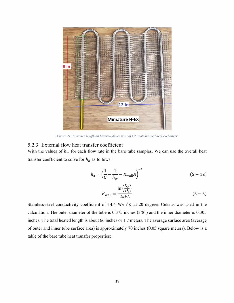
37

Figure 24: Entrance length and overall dimensions of lab scale meshed heat exchanger

5.2.3 External flow heat transfer coefficient With the values of ℎ𝑤 for each flow rate in the bare tube samples. We can use the overall heat

transfer coefficient to solve for ℎ𝑎 as follows:

ℎa = (1

𝑈−

1

ℎw− 𝑅wall𝐴)

−1

(5 − 12)

𝑅wall =ln (

𝐷o

𝐷i)

2𝜋𝑘𝐿(5 − 5)

Stainless-steel conductivity coefficient of 14.4 W/m2K at 20 degrees Celsius was used in the

calculation. The outer diameter of the tube is 0.375 inches (3/8”) and the inner diameter is 0.305

inches. The total heated length is about 66 inches or 1.7 meters. The average surface area (average

of outer and inner tube surface area) is approximately 70 inches (0.05 square meters). Below is a

table of the bare tube heat transfer properties:

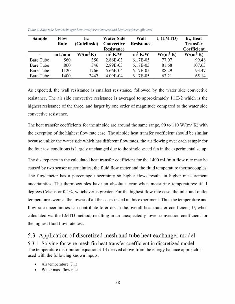
38

Table 6: Bare tube heat exchanger heat transfer resistances and heat transfer coefficients

Sample Flow

Rate

hw

(Gnielinski)

Water Side

Convective

Resistance

Wall

Resistance

U (LMTD) ha, Heat

Transfer

Coefficient

- mL/min W/(m2 K) m2 K/W m2 K/W W/(m2 K) W/(m2 K)

Bare Tube 560 350 2.86E-03 6.17E-05 77.07 99.48

Bare Tube 860 346 2.89E-03 6.17E-05 81.68 107.63

Bare Tube 1120 1766 5.66E-04 6.17E-05 88.29 93.47

Bare Tube 1400 2447 4.09E-04 6.17E-05 63.21 65.14

As expected, the wall resistance is smallest resistance, followed by the water side convective

resistance. The air side convective resistance is averaged to approximately 1.1E-2 which is the

highest resistance of the three, and larger by one order of magnitude compared to the water side

convective resistance.

The heat transfer coefficients for the air side are around the same range, 90 to 110 W/(m2 K) with

the exception of the highest flow rate case. The air side heat transfer coefficient should be similar

because unlike the water side which has different flow rates, the air flowing over each sample for

the four test conditions is largely unchanged due to the single speed fan in the experimental setup.

The discrepancy in the calculated heat transfer coefficient for the 1400 mL/min flow rate may be

caused by two sensor uncertainties, the fluid flow meter and the fluid temperature thermocouples.

The flow meter has a percentage uncertainty so higher flows results in higher measurement

uncertainties. The thermocouples have an absolute error when measuring temperatures: ±1.1

degrees Celsius or 0.4%, whichever is greater. For the highest flow rate case, the inlet and outlet

temperatures were at the lowest of all the cases tested in this experiment. Thus the temperature and

flow rate uncertainties can contribute to errors in the overall heat transfer coefficient, U, when

calculated via the LMTD method, resulting in an unexpectedly lower convection coefficient for

the highest fluid flow rate test.

5.3 Application of discretized mesh and tube heat exchanger model

5.3.1 Solving for wire mesh fin heat transfer coefficient in discretized model The temperature distribution equation 3-14 derived above from the energy balance approach is

used with the following known inputs:

• Air temperature (𝑇∞)

• Water mass flow rate

39

• Water specific heat

• Bare tube overall heat transfer

• Bare tube cross section perimeter

• Section length

• Fin perimeter (wire circumference)

• Find conductivity (stainless steel)

• Cross section area of fin (wire cross section area)

• Length of fin (longitudinal and transverse wire lengths)

• Distances of transverse fins along longitudinal fin

• Measured inlet temperature

Using the Microsoft Excel data analysis tool: Solver, the measured outlet temperature is the

target reached by adjusting the fin heat transfer coefficient value, the following results were

generated:

Table 7: Model predicted heat transfer coefficients for meshed heat exchangers assuming perfect fin to tube contact

Sample Flow

Rate

hmodel

- mL/min W/(m2 K)

500 in/min, Rectangular Pattern, Thin Coating 560 203








500 in/min, Rectangular Pattern, Thick Coating 560 24902




500 in/min, Linear Pattern, Medium Coating 560 11412




The model predictions for apparent fin heat transfer coefficient shows a high degree of variation

for the thicker coating samples. But as with the aforementioned bare tube case, the air side heat

transfer coefficient should stay roughly identical for each sample because air speed and

temperature were largely the same. These fin heat transfer coefficients are classified as “apparent”

because the true heat transfer performance of the fins should not vary much between the samples

as all of them use the same fins; the same wire mesh dimensions, same number of mesh layers (2),

40

same pore sizes (4 PPI), and finally the same wire diameters (0.81 mm). Thus, what remains

different between the samples is the thermal sprayed coating. The difference in heat transfer

coefficient is caused by the difference in conductive resistance in the thermal sprayed coating

which affects the heat transfer between the mesh and tube.

5.3.2 Prediction of outlet water temperature with average air side heat transfer

coefficient in discretized model The model is more accurate when used in predicting the outlet temperature instead of solving for

heat transfer coefficient. The model temperature outputs are not as varied as the previous heat

transfer coefficient outputs. The following is a chart of the outlet temperature prediction by taking

the average (with the outlier value removed) of the heat transfer coefficients.

The outlier for each sample’s heat transfer coefficient is removed in accordance to the Chauvenet’s

criterion as it was determined that the chance for a data point to be as deviant as the outlier were

less than half of one measurement from four measurements [46]. By removing the outlier, the

standard deviation for each sample decreased to at least 1/3 of the value before removing the

outlier. It is assumed that the data collected were normally distributed but due to the low number

of data points, the uncertainty of the mean and standard deviation from their true values remains

high. Collecting more data points would result in less uncertainty and more confidence in applying

Chauvenet’s criterion to reject outlier data.

41

Table 8: Apparent average heat transfer coefficients for meshed heat exchangers and predicted outlet temperature accuracy

Sample Flow

Rate

Toutlet Average

hmodel*

Model

predicted

Toutlet

% Error

(+ over, -

under)

- mL/min ℃ W/(m2 K) ℃ -

500 in/min, Rect. Pattern, Thin Coating 560 29.9

118

29.2 -2.2%

500 in/min, Rect. Pattern, Thin Coating 860 24.6 24.6 0.2%


500 in/min, Rect. Pattern, Thin Coating 1400 17.2 17.0 -1.1%

1000 in/min, Rect. Pattern, Thin Coating 560 35.0

285

31.3 -10.5%



1000 in/min, Rect. Pattern, Thin Coating 1400 19.0 18.8 -1.1%

500 in/min, Rect. Pattern, Thick Coating 560 51.4

8146

41.3 -19.7%

500 in/min, Rect. Pattern, Thick Coating 860 39.7 37.4 -5.9%

500 in/min, Rect. Pattern, Thick Coating 1120 33.5 35.2 5.1%

500 in/min, Rect. Pattern, Thick Coating 1400 27.9 28.9 3.4%

500 in/min, Lin. Pattern, Med. Coating 560 38.5

2029

31.4 -18.4%

500 in/min, Lin. Pattern, Med. Coating 860 27.6 26.7 -3.4%

500 in/min, Lin. Pattern, Med. Coating 1120 22.6 24.3 7.5%

500 in/min, Lin. Pattern, Med. Coating 1400 22.1 21.7 -1.8%

* Outlier removed

It can be observed that the model predicts more accurately, the outlet temperatures of the higher

water flowrate cases. The lowest water flow rate (560 mL/min) for each case exhibits consistently

larger percent error in predicted outlet temperature compared to the other flow rate cases. One

source of error could be air bubbles in the water. At the lowest flowrate, by inspection through the

semi-transparent housing of the turbine flow meter, air bubbles were present. Two-phase flow

changes heat transfer characteristics. Two possible explanations for two-phase flow are low

pressure throttling effect (cavitation) from the throttling valve upstream of the sample and

localized vaporization during low flow rates at disturbances on the tube inner wall or hotspots.

Vapor bubbles from the boiling causes two phase flow. The discretized model was not developed

to account for two phase flow. In order to account for the localized vaporization, pinch point

analysis may be utilized to find the two-phase flow heat transfer coefficient. This was not

investigated in the present study.

5.4 One-dimension heat transfer Biot approximation In order to make the fin approximation for the wire mesh, the Biot number is checked to verify

that the fin has a constant cross section temperature at any point. This approximation simplifies

42

the steady state heat transfer equation into one dimension and can simplify non-uniform cross

sections. Although in the wire mesh case, the wires are assumed to be constant cross section. The

Biot number is a ratio of the internal conduction resistance and the external convection resistance

of the geometry. If the Biot number is much smaller than unity, this indicates that the internal

conduction resistance is less than the external convection resistance and therefore the fin

approximation is possible. The equation is as follows:

𝐵𝑖 =ℎ𝛿

𝑘≪ 1 (5 − 16)

Where ℎ is the convective heat transfer coefficient, 𝛿 is half the thickness of the fin (radius of the

cylindrical wire), 𝑘 is the thermal conductivity of the fin material (stainless steel). In the case of

the wire mesh, the Biot number is 0.2, slightly over the accepted value of 0.1 when the

simplification is justified. The accuracy of the fin approximation can be improved with a more

conductive material such as copper or aluminum, a thinner wire, or in operating cases where the

airflow decreases the heat transfer coefficient.

5.5 Infinite fin approximation and effective fin length The resulting heat transfer coefficient will also be used to check if the infinite fin approximation

is valid.

𝑞finite fin

𝑞infinite fin=

√ℎ𝑃𝑘𝐴c(𝑇∞ − 𝑇b) tanh 𝑚𝐿

√ℎ𝑃𝑘𝐴c(𝑇∞ − 𝑇b)= tanh 𝑚𝐿 (5 − 17)

To do so, we inspect the value of 𝑚𝐿, 𝑚2 =ℎ𝑃

𝑘𝐴c, where 𝐿 is the fin length and 𝑚 depends on the

fin cross section area, cross section perimeter, material thermal conductivity, and heat transfer

coefficient. When 𝑚𝐿 is greater than 2.5, tanh 𝑚𝐿 is greater than 0.9 meaning the finite fin is

over 90% what an infinite length fin (with all the other fin properties the same) would perform in

terms of heat transfer. At about 𝑚𝐿 = 5, tanh 𝑚𝐿 = 1, so the finite fin heat transfer rate is same

as an infinite fin.

To extend this concept, we can calculate the optimal length for the fins such that the finite length

fin performs essentially identically to an infinite length fin of the same cross section geometry. For

the case of the lab scale heat exchangers, the convective heat transfer coefficient is greater than

8000 W/m2 K. With the perimeter, cross section area, thermal conductivity known, the value of 𝑚

43

is over 1600 m-1. If 𝑚𝐿 = 5 is when the finite fin heat transfer rate is the same as an infinite fin of

the same cross section and geometry, then we can find 𝐿.

5

𝑚= 𝐿 (5 − 18)

𝐿 ≈ 0.003 m (5 − 19)

Thus, the effective fin length is 3 mm. The first set of transverse fins is located at 3.175 mm (0.125

inch) along the longitudinal fin. Therefore, according to the heat transfer model, they are not as

effective because there are no longer any large temperature gradients at that point on the

longitudinal fin. The transverse fin tips for each unit cell are also assumed to be insulated and reach

the air temperature. From the above effective length calculation, the assumption is reasonable since

the wire mesh wire fins reach the air temperature around 3 mm whereas the transverse fins are

over 3 mm long. Plots of the fin model temperature distributions are generally in agreement with

the above calculation as fin temperatures have reached the air temperature around 3 mm away

from the base. The plots of fin temperatures are shown below.

Figure 25: Temperature distribution along longitudinal fin, thinly coated (<1 mm) sample

0

50

100

150

200

250

0 0.002 0.004 0.006 0.008 0.01

Tem

per

atu

re [

℃]

Length from Base of Fin [m]

44

Figure 26: Temperature distribution along longitudinal fin, medium thickness (>1 mm) coating

5.6 Coating thickness In total, four samples were fabricated in order to compare the different coating impacts on heat

transfer performance. The samples with coating thicknesses slightly larger than the wire diameter

(0.81 mm) are referred to as thin samples. The medium sample coating thickness is around 1 mm

in thickness. The thick sample has a coating thickness of over 1.2 mm. The following table lists

the coatings thicknesses which were deposited:

Table 9: All samples produced and corresponding coating thicknesses

Sample Coating

Thickness

[mm]

Bare Tube -

500 in/min, Linear Trajectory Pattern 1.04

1000 in/min, Rectangular Trajectory Pattern 0.87



5.6.1 Coating cross section Wire-arc sprayed test pieces were cut with a diamond bladed linear precision saw (IsoMet 4000,

BUEHLER LTD, IL, USA). Resin mounted samples were made and polished with an automated

sample grinder (EcoMet 300, BUEHLER LTD, IL, USA). Settings and materials used for

polishing are listed in the two tables below.

0

50

100

150

200

250

0 0.002 0.004 0.006 0.008 0.01

Tem

per

atu

re [

℃]

Length from Base of Fin [m]

45

Table 10: Polishing settings for sample preparation (machine specific)

Polishing

Settings

Sandpaper Grit

Succession

100 rpm base 240

60 rpm head 320

Counterrotation 400

With water 600

6 lb. force 1200

The following images of wire and tube cross sections were taken with a tabletop SEM (TM3000,

Hitachi High-Tech Corp. Fukuoka, Japan). The cross-section area where the wire is in contact with

the tube is the main area of interest.

Figure 27: Various tube, coating and mesh wire cross sections: high speed rectangular trajectory thin coating with extended

gaps (Top Left), high speed rectangular trajectory thin coating with void between tube and wire (Top Right), low speed linear

trajectory medium coating with void (Bottom Left), and low speed rectangular trajectory thick coating with void (Bottom Right)

As can be seen in the images above, it is common to have a slight void between the wire and tube

surface for all coating thicknesses. Any voids are not ideal for heat transfer performance as they

increase contact resistance between the wire and the tube. The cause of this space was initially

thought to be insufficiencies from the clamping method which left gaps between the mesh and

tube. But after several cross-section cuts from various locations on the test samples, and various

46

attempts at ensuring the clamping method set the mesh flush with the tube before coating, the void

still persists. For the worst cases, as in the top left SEM image above, not only are voids present

between the wire and the tube, the coating has gaps which could be prone to wire and coating

delamination.

A thicker coating may reduce the contact resistance detriment to heat transfer because the coating

thickness offers alternative paths of heat conduction. This is reflected in the performance of the

coated tube and mesh heat exchangers. Thicker coatings resulted in higher temperature differences

compared to thinner coated samples.

47

5.7 Thermal sprayed coating conductive resistance In order to compare the coating performance of the four coated samples, the average apparent heat

transfer coefficient calculated from the thickest coated heat exchanger sample is used as the fin

heat transfer coefficient for all samples with the assumption of perfect contact between the mesh

fins and bare tube. Thus, all other samples with thinner coating and different coating application

settings must exhibit a temperature difference between the base of the fin and the surface of the

tube. This temperature difference is caused by the conductive resistance in the thermal sprayed

coating bonding mesh wire to bare tube. To quantify the value of the coating conductive resistance,

the resistance network analogy can be utilized. Below is a diagram illustrating the coating as part

of the heat transfer pathway:

Figure 28: Thermal resistance network for meshed tubular heat exchanger

Thermal resistance can be defined by the following equation:

48

�̇� =∆𝑇

𝑅(5 − 2)

For the coating resistance, we have:

𝑅coating =𝑇fin base − 𝑇tube outer

�̇�fin

(5 − 20)

𝑇fin base − 𝑇tube outer = 𝑇difference (5 − 21)

From the previously developed discretized model, a constant temperature difference term is added

to the fin equations since the fin base temperature is no longer equivalent to the water temperature

within the tube as perfect contact is no longer the assumption. The convective resistance of the air

side and conductive resistance within the fin wire elements are accounted for in the fin equations.

The bare tube model considers the conductive resistance of the tube wall and convective resistance

of the water flowing inside the tube. Thus the temperature difference between the fin base and tube

surface should represent the coating conductive resistance.

Thus, assuming a constant temperature difference between the fin base temperature and the tube

surface temperature, a solver is used to find the temperature difference with known heat transfer

coefficient, inlet / outlet temperatures, and fin parameters. The heat transfer rate in equation 5-20

is calculated by summing the fin heat transfer rates across the whole sample (all of the 192

discretized segments).

The table below shows the temperature differences for each sample and the calculated average

wall resistance across the whole heat exchanger. Note that since the thick coating was considered

to be in perfect contact with the tube, the temperature difference between the mesh wire fins and

tube is zero by definition. Thus all results are relative comparisons to the thick coating sample.

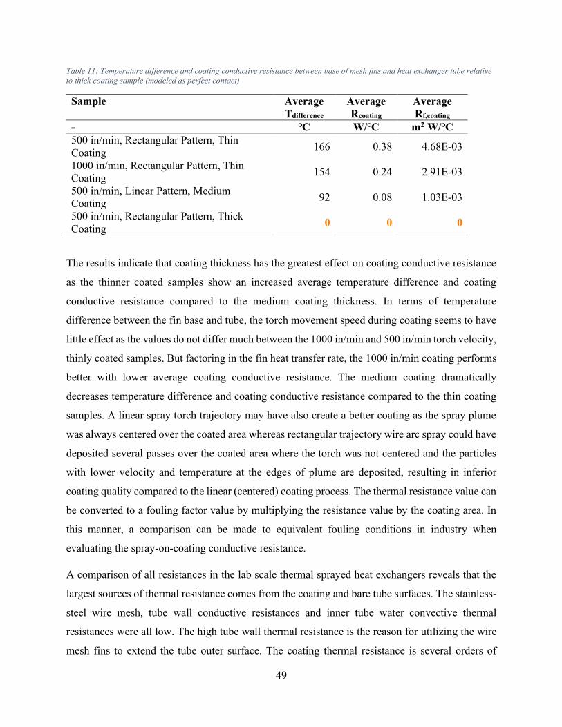
49

Table 11: Temperature difference and coating conductive resistance between base of mesh fins and heat exchanger tube relative

to thick coating sample (modeled as perfect contact)

Sample Average

Tdifference

Average

Rcoating

Average

Rf,coating

- ℃ W/℃ m2 W/℃

500 in/min, Rectangular Pattern, Thin

Coating 166 0.38 4.68E-03

1000 in/min, Rectangular Pattern, Thin

Coating 154 0.24 2.91E-03

500 in/min, Linear Pattern, Medium

Coating 92 0.08 1.03E-03

500 in/min, Rectangular Pattern, Thick

Coating 0 0 0

The results indicate that coating thickness has the greatest effect on coating conductive resistance

as the thinner coated samples show an increased average temperature difference and coating

conductive resistance compared to the medium coating thickness. In terms of temperature

difference between the fin base and tube, the torch movement speed during coating seems to have

little effect as the values do not differ much between the 1000 in/min and 500 in/min torch velocity,

thinly coated samples. But factoring in the fin heat transfer rate, the 1000 in/min coating performs

better with lower average coating conductive resistance. The medium coating dramatically

decreases temperature difference and coating conductive resistance compared to the thin coating

samples. A linear spray torch trajectory may have also create a better coating as the spray plume

was always centered over the coated area whereas rectangular trajectory wire arc spray could have

deposited several passes over the coated area where the torch was not centered and the particles

with lower velocity and temperature at the edges of plume are deposited, resulting in inferior

coating quality compared to the linear (centered) coating process. The thermal resistance value can

be converted to a fouling factor value by multiplying the resistance value by the coating area. In

this manner, a comparison can be made to equivalent fouling conditions in industry when

evaluating the spray-on-coating conductive resistance.

A comparison of all resistances in the lab scale thermal sprayed heat exchangers reveals that the

largest sources of thermal resistance comes from the coating and bare tube surfaces. The stainless-

steel wire mesh, tube wall conductive resistances and inner tube water convective thermal

resistances were all low. The high tube wall thermal resistance is the reason for utilizing the wire

mesh fins to extend the tube outer surface. The coating thermal resistance is several orders of

50

magnitude higher than all thermal resistances other than bare tube convective thermal resistance

and is a bottleneck to the fin heat transfer, somewhat mitigating the heat transfer enhancement that

the fins provide.

Coating thermal resistance can be broken down into two contact resistances, the mating surfaces

between the mesh wire and the coating as well as the mating surfaces between the coating and the

tube surface. Furthermore, the coating layer has a conductive resistance. Further studies are

required to better determine the magnitudes of the surface interface thermal resistances and the

internal conductive thermal resistance of the coating.

Table 12: Comparison of thermal resistance values in the heat exchanger thermal resistance network

Thermal Resistance Value or Range

[℃/W]

Bare Tube (Convective) 0.2

Fin (Convective) 0.002

Coating (Conductive) 0.08 - 0.38

Tube Wall (Conductive) 0.001

Inner Tube (Convective) 0.009 - 0.07

5.7.1 Effects of high temperature gradient areas due to high thermal resistances By design, the materials in the tube, mesh and coating are all stainless steel in order to avoid

uneven thermal expansion due to material property differences, leading to coating failure. Despite

similar material properties, uneven heating and high temperature differentials across the sample

can still cause uneven thermal expansions leading to coating failure. As previously discussed,

thinner coatings have a greater thermal resistance than thicker coatings. The temperature different

between the mesh fin tip and base is higher than thicker coatings.

It is suspected that the thinner coating structural strength is lower than the medium or thick coating

and due to uneven heating, the hotspot area mesh and coating experiences more thermal expansion

compared to the surrounding material. These factors are compounded by the thermal resistance in

the coating causing even greater localized temperature differences. Increased thermal expansion

force caused the coating and mesh to buckle upwards, away from the tube surface. Uneven heating

is caused by the fan creating flame vortices at the center of the duct resulting in hotter air at the

center than the edges. This is evident in the following image where a circular shape (annotated

with a blue circle) is noticeable at the center of the meshed sample.

51

Figure 29: Unevenly heated center of wire mesh heat exchanger

After several rounds of testing, each sample was subjected to at least 10 minutes of continuous

heating by air approaching an average temperature of 300℃. Hot spots were measured to be

upwards of 600℃. Tests were completed with both water flowing through the heat exchanger tubes

and while they were dry. The only sample which failed by delamination of coating from tube was

the high-speed (1000 in/min torch tip speed) thin coating. The picture below shows the area where

the coating failed.

Figure 30: Coating delamination from tube surface, showing gap between mesh and tube

Avoiding uneven heating during operation and using thicker coatings would increase the heat

exchanger durability. Running the heating system while the heat exchanger has no water flowing

within also puts the materials at greater stresses due to the higher temperatures reached. Thus, any

52

field application should require the flare or flue stack startup to be linked directly with fluid pumps

feeding the heat exchanger, to ensure that whenever hot air passes through the stack, water is

flowing inside the heat exchanger.

5.8 Heat transfer rate for finned vs. bare tube heat exchangers The surface area of the wire mesh fins is coincidentally the same surface area as the tube within

heated section of the duct at around 0.05 square meters. The convective heat transfer coefficient

of the wire mesh extended surface is much higher than the bare tube (8000 vs. 100 W/m2K) which

in indicative that at the same temperature difference, the fins enhance the rate of heat transfer

greatly compared to a bare tube. But despite the greatly increased heat transfer coefficient, the

actual resulting water temperature difference inside of the meshed and bare tube samples do not

reflect the large difference between the two heat transfer coefficients on the outer surfaces of the

tube. This is in part due to the thermal resistances in other parts of the heat transfer network. There

are locations in the heat transfer network which bottleneck the heat transfer.

As can be seen in the following table of average heat transfer for each sample calculated from the

water flow rate and water temperature difference between the inlet and outlet, the wire mesh

nonetheless does improve the heat transfer rate for each of the coated samples.

Table 13: Average heat transfer rate comparison table

Sample Avg. Heat

Transfer Rate

[W]

%

Improvement

Over Bare Tube

Bare tube 569 -

500 in/min, Rectangular Pattern, Thin Coating 789 39%

1000 in/min, Rectangular Pattern, Thin Coating 935 64%

500 in/min, Linear Pattern, Medium Coating 1115 96%

500 in/min, Rectangular Pattern, Thick Coating 1807 217%

The large difference in heat transfer rate between the coated sample are indicative of differences

in heat transfer rates between the samples which are due to differences in the thermal sprayed

coatings and subsequent differences in airflow caused by the coatings. All other parameters of the

samples were kept the same such as: meshed area, layers of mesh, mesh wire geometry, wire mesh

connections, tube length, tube diameter, water / air flowrates, and water inlet / air temperatures.

The thicker coated sample decreased wire mesh porosity which reduced the airflow speed (less

53

than 5 m/s), accumulating hot air upstream of the sample, causing the sample to heat water to much

higher temperatures compared to the other samples. Air speed for the other three coated samples

were relatively similar (approximately 6 m/s). The unmeshed bare tube sample had least

obstruction to airflow, evident in the highest measured airflow velocity of 8 m/s.

Thus, not only does the thicker coating accumulate heated air upstream of the sample, it also has

lower thermal resistances compared to the thinner coatings. Therefore the performance of the thick

coated mesh and tube heat exchanger is significantly better than thin or unmeshed samples.

54

6 Conclusions and future work

6.1 Conclusion Mesh and tube heat exchangers were fabricated and thermal spray coating was applied to bond the

mesh to tube. From previous studies, it was observed that mesh to tube contact area was limited.

Potential to increase heat transfer rate and structural integrity between the mesh and tube remained

by using thicker thermal sprayed coating. To increase mesh to tube contact area and provide a

larger area for thermal sprayed coating application, the tube surfaces which are connected to the

wire mesh are flattened with a custom designed press. Coating thickness was increased enough to

fully embed the wire mesh onto the tube under the thermally sprayed coating.

Samples were placed inside a custom designed duct, fan and propane torch air heating system. The

resulting temperature difference between the water inlet and outlet was 1.5 to 4 times greater than

achieved in a previous study. Temperature difference trends at different water flow rates were in

line with the previous study. Heat transfer rates, calculated from water inlet and outlet temperature

differences, were enhanced by at least 39% and up to 217% compared to bare tube samples after

the addition of thermal sprayed mesh. Air side heat transfer coefficient was predicted to have

increased by 40 to 80 times from bare tube to mesh and coated tubes. Unfortunately, the magnitude

of heat transfer enhancements on the air side is not translated to the same magnitude of heat transfer

into the water inside the tube. This was due to thermal resistances in the coating which bonds the

mesh to the tube.

Using the inlet temperature and heated air properties as inputs, a discretized model was developed

to predict outlet temperatures. The air side convective heat transfer coefficient is adjusted such

that the model predicts an outlet water temperature comparable to experimental data to within 20%

error, and less than 8% error if the lowest flowrate data is omitted for each sample due to the

possible presence of two phase flow. An apparent convective heat transfer coefficient was

calculated, ranging from several hundred to several thousand W/m2 K.

The large range in the apparent heat transfer coefficient can be explained by coating differences

between the samples. By assuming that the best performing, thickest coated sample had minimal

thermal resistance, its heat transfer coefficient was applied to all samples tested and deemed as the

air side convective heat transfer coefficient. The aforementioned model is further developed with

the addition of a temperature difference to predict the coating thermal resistance. It was found that

55

the largest contribution to thermal resistance was coating thickness. Spray trajectory and torch tip

velocities may have caused a difference in coating quality, but their effect was not large enough to

cause a noticeable difference in heat transfer performance, when compared to coating thickness.

A thicker coating can decrease conductive thermal resistances by 1 to 2 orders of magnitude. The

convective resistance of bare tube is also reduced by 2 orders of magnitude with the addition of

wire mesh fins. Tube wall conductive resistance is insignificant compared to the other sources of

thermal resistance in the heat transfer network.

Fin temperature distributions also indicate that fin temperature gradients are only present in the

first 3 to 4 mm of the wire mesh fin. As such, the majority of the fin lengths and cross fins do not

contribute to the heat transfer performance of the lab-scale samples.

6.2 Future work

6.2.1 Improvements on sources of measurement uncertainty / error Each lab-scale heat exchanger was tested at four water flow rates. Each test was run only once, for

a total of 20 tests. To determine the air-side heat transfer coefficient, only four data points were

usable for each sample. This low sample size, in addition to each sample being at a different water-

side flow rate, has high uncertainty. Chauvenet’s criterion was used, but the mean and standard

deviations from the four data points is highly uncertain. More data points would result in higher

statistical significance and enable confirmation of the normal distribution assumed when using the

aforementioned criterion.

A potential source for uncertainties is in the water temperature measurement. Thermocouples used

had a tolerance range of 2.2℃. This meant that measuring small temperature differences between

inlet and outlet had a high degree of uncertainty. Improved thermocouples with smaller

uncertainties could be utilized, but because the thermocouples are unique with probe tips and

threads designed for NPT threaded ports and submersion, this may prove challenging. Calibration

of existing thermocouples may be a more feasible option.

Airflow inside the duct also tended to be concentrated in a toroidal shape due to the vortex

generated from the axial fan blade rotation and airflow dead-zone at the center due to the blade

center hub obstructing airflow. This was apparent in temperature measurements as the central area

was much hotter than the corners or sides of the duct. Similar airflow pattern was also measured

using the pitot tube when determining the airflow velocity. Lastly, scorch marks on the wire mesh

56

for each sample show a clear toroidal cross section imparted onto the sample after testing. The

average air temperature in the duct was determined with 12 equally spaced measurement points.

To improve the uniformity of the duct cross section temperatures, flow straightener(s) and metal

foam layer(s) could be used upstream in the duct to ensure the airflow is mixed and straightened

before reaching the sample. Consideration for pressure drop is required to ensure sufficient flow

velocity for a forced convection heat transfer system. Canarm supplies fans with in-kind

dimensions and higher horsepower motors to provide more airflow.

6.2.2 Improvements on testing capability Testing was done with a fixed speed fan and lowest propane pressure settings for the air heating

torch. Future tests could feature multiple airflow set points and increased air temperatures. Altering

the airflow can give further insight into the air side heat transfer coefficient of the mesh wire fins.

Temperatures were kept low in order to protect the samples in order that they were not destroyed

before any data was collected. During tests, air temperatures were below 300℃, but preliminary

tests show that the setup is capable of up to 700℃ air at the duct outlet. Propane torch pressures

can be increased in order to achieve higher air temperatures.

Lastly, the capabilities of the fan, duct and, torch setup are such that it may be possible to direct

the duct outlet onto the crossflow surface area of the large-industrial scale prototype which had

previously been too large to test with existing systems. Details of the previous attempted at testing

the industrial scale prototype are provided in Appendix A. Given high speed airflow and high

temperatures made possible by using a propane torch system, the industrial scale heat exchanger

may finally be subjected to enough high temperature airflow such that it produces a significant

temperature difference in the fluid contained within the tubes.

6.2.3 Improvements on mathematical modelling Furthermore, the completed model could be used to compute results from former experiments in

Rezaey’s work [28]. The tests done previously featured different mesh geometries and pore

densities. The temperature data from those tests would serve to validate the model further and

expand the model’s applicability in predicting outlet temperatures or heat transfer coefficients of

different mesh geometries and layouts. A determination of thermal sprayed coating thermal

resistance is also useful to compare the thinly coating samples from Rezaey’s work to the thicker

coatings fabricated in the present study.

57

6.2.4 Future investigation into coating thermal resistances Given that coating difference account for a large part of the thermal resistance in the heat

exchanger samples, greater detail should be placed upon investigation of coating internal

conductive resistances and contact resistances. The lumped coatings resistance values presented

in section 5.6 do not separate the multiple thermal resistances within the mesh wire to coating to

tubing interfaces. There are at least three thermal resistances in that subsystem which require

further investigation. Contact resistances between the wire mesh and coating, due to imperfections

in the bond surfaces between wire and coating. Conductive resistances within the coating volume

which may be affected by coating porosities. Contact resistance between the coating and the tube

as illustrated by the voids in the cross-section SEM images provided in section 5.6.1.

6.2.5 Future design considerations for mesh fins Since the mesh fin temperature distribution shows that only the initial 3 to 4 mm from the base of

the fin have a significant temperature gradient, future designs may consider utilizing less mesh

area. This offers the possibility to arrange the tube in denser packed geometries as less space is

required for the extended surfaces. This gives way to higher performance designs with longer tube

length fitting within a smaller heated area, decreases weight, more compact designs, and greater

fin efficiency.

58

References [1] B. Zohuri, Compact Heat Exchangers, 1st ed. Springer International Publishing, 2017.

[2] Thermopedia, “Heat Exchangers,” 2011. http://www.thermopedia.com/content/832/ (accessed

Apr. 05, 2020).

[3] S. P. Sukhatme and S. Devotta, “Classification of Heat Transfer Equipment,” in Heat Transfer

Equipment Design, R. K. Shah, E. C. Subbarao, and R. A. Mashelkar, Eds. Taylor & Francis,

1988, pp. 7–15.

[4] D. P. Sekulić and R. K. Shah, Fundamentals of Heat Exchanger Design, 1st ed. John Wiley &

Sons, Inc., 2003.

[5] S. S. Mehendale, “Single-Phase Heat Exchangers,” in Handbook of Thermal Science and

Engineering, F. A. Kulacki, Ed. Springer, Cham, 2017.

[6] K. Thulukkanam, Heat Exchanger Design Handbook, 1st ed. CRC Press, 2000.

[7] Natural Resources Canada, “Crude oil facts,” 2020. https://www.nrcan.gc.ca/science-data/data-

analysis/energy-data-analysis/energy-facts/crude-oil-facts/20064 (accessed Mar. 21, 2020).

[8] United States Environmental Protection Agency, “AP 42, Fifth Edition Compilation of Air

Pollutant Emissions Factors, Volume 1: Stationary Point and Area Sources - Section 13.5 -

Industrial Flares,” 2018.

[9] United States Environmental Protection Agency, “CATC Air Pollution Technology Fact Sheet -

Flare,” 2003.

[10] M. E. Mondejar, J. G. Andreasen, L. Pierobon, U. Larsen, M. Thern, and F. Haglind, “A review of

the use of organic Rankine cycle power systems for maritime applications,” Renew. Sustain.

Energy Rev., vol. 91, no. March, pp. 126–151, 2018, doi: 10.1016/j.rser.2018.03.074.

[11] M. A. Khatita, T. S. Ahmed, F. H. Ashour, and I. M. Ismail, “Power generation using waste heat

recovery by organic Rankine cycle in oil and gas sector in Egypt: A case study,” Energy, vol. 64,

pp. 462–472, 2014, doi: 10.1016/j.energy.2013.11.011.

[12] R. Mudasar, F. Aziz, and M. H. Kim, “Thermodynamic analysis of organic Rankine cycle used for

flue gases from biogas combustion,” Energy Convers. Manag., vol. 153, no. October, pp. 627–

640, 2017, doi: 10.1016/j.enconman.2017.10.034.

[13] Fernando B. Mainier, Marcone F. Reis, Fabiano R. C. Nunes, and Annelise Zeemann, “Impact of

Deterioration of Flare of an Offshore Oil Platform,” J. Mater. Sci. Eng. B, vol. 6, no. 1, Feb. 2016,

doi: 10.17265/2161-6221/2016.1-2.003.

[14] I. Taie, A. Al-Shahrani, N. Qari, A. Fihri, W. Al-Obaid, and G. Alabedi, “High temperature

corrosion resistant coatings for gas flare systems,” Ceram. Int., vol. 44, no. 5, pp. 5124–5130, Apr.

2018, doi: 10.1016/J.CERAMINT.2017.12.114.

[15] D. E. Crawmer, “Coating Structures, Properties, and Materials,” in ASM Handbook, Volume 5A:

Thermal Spray Technology, J. Robert C. Tucker, Ed. ASM International, 2013.

[16] L. Pawlowski, The Science and Engineering of Thermal Spray Coatings, 2nd ed. John Wiley &

Sons, 2008.

[17] C. U. Hardwicke and Y. C. Lau, “Advances in thermal spray coatings for gas turbines and energy

generation: A review,” J. Therm. Spray Technol., vol. 22, no. 5, pp. 564–576, 2013, doi:

59

10.1007/s11666-013-9904-0.

[18] J. C. Tan, L. Looney, and M. S. J. Hashmi, “Component repair using HVOF thermal spraying,” J.

Mater. Process. Technol., vol. 92–93, pp. 203–208, 1999, doi: 10.1016/S0924-0136(99)00113-2.

[19] V. Champagne and D. Helfritch, “Critical Assessment 11: Structural repairs by cold spray,”

Mater. Sci. Technol. (United Kingdom), vol. 31, no. 6, pp. 627–634, 2015, doi:

10.1179/1743284714Y.0000000723.

[20] A. Kutay and L. Weiss, “Economic Impact of Automation: The Case of Robotic Thermal

Spraying,” Pittsburgh, 1990. doi: 10.1017/CBO9781107415324.004.

[21] S. Deng, D. Fang, Z. Cai, H. Liao, and G. Montavon, “Application of external axis in robot-

assisted thermal spraying,” J. Therm. Spray Technol., vol. 21, no. 6, pp. 1203–1215, 2012, doi:

10.1007/s11666-012-9818-2.

[22] W. Goetzler, M. Guernsey, and J. Young, “Opportunities for Joining Technologies in HVAC &

R,” 2015.

[23] Kermetico Inc., “HVAF Alloy Coatings to Protect Petrochemical Heat Exchangers from H₂S and

CO₂ Corrosion,” 2013. https://kermetico.com/applications/hvaf-alloy-coatings-protect-

petrochemical-heat-exchangers-h2s-co2-corrosion (accessed Mar. 24, 2020).

[24] H. Wilson, R. Johnsen, I. Co-Supervisor:, and A. Barnoush, “Thermal Sprayed Aluminium for

Subsea Heat Exchanger Surfaces Effect of Temperature on Protection Current Requirement and

Calcareous Development,” The Norwegian University of Science and Technology, 2014.

[25] P. Hafeez, S. Chandra, and J. Mostaghimi, “Heat transfer during high temperature gas flow

through metal foam heat exchangers,” J. Heat Transfer, vol. 139, no. 12, pp. 1–11, 2017, doi:

10.1115/1.4037082.

[26] P. Hafeez, S. Yugeswaran, S. Chandra, J. Mostaghimi, and T. W. Coyle, “Fabrication of High-

Temperature Heat Exchangers by Plasma Spraying Exterior Skins on Nickel Foams,” J. Therm.

Spray Technol., vol. 25, no. 5, pp. 1056–1067, 2016, doi: 10.1007/s11666-016-0413-9.

[27] J. Assaad, A. Corbeil, P. F. Richer, and B. Jodoin, “Novel stacked wire mesh compact heat

exchangers produced using cold spray,” J. Therm. Spray Technol., vol. 20, no. 6, pp. 1192–1200,

2011, doi: 10.1007/s11666-011-9663-8.

[28] R. Rezaey, “Experimental Investigation of Heat Transfer and Fluid Flow in Laser Sintered Heat

Exchangers,” University of Toronto, 2017.

[29] R. Rezaey, S. Salavati, L. Pershin, T. Coyle, S. Chandra, and J. Mostaghimi, “Fabrication of wire

mesh heat exchangers for waste heat recovery using wire-arc spraying,” J. Therm. Spray Technol.,

vol. 23, no. 4, pp. 609–615, 2014, doi: 10.1007/s11666-014-0058-5.

[30] Y. Fu, J. Wen, and C. Zhang, “An experimental investigation on heat transfer enhancement of

sprayed wire-mesh heat exchangers,” Int. J. Heat Mass Transf., vol. 112, pp. 699–708, 2017, doi:

10.1016/j.ijheatmasstransfer.2017.05.026.

[31] L. S. Tong and A. L. London, “HEAT-TRANSFER AND FLOW-FRICTION

CHARACTERISTICS OF WOVEN-SCREEN AND CROSSED- ROD MATRIXES,” Trans. Am.

Soc. Mech. Eng., vol. Vol: 79, 1957.

[32] C. Li and R. A. Wirtz, “Development of a High Performance Heat Sink Based on Screen-Fin

Technology,” Reno, 2003. doi: 10.1109/STHERM.2003.1194339.

60

[33] W. S. Chang, “Porosity and Effective Thermal Conductivity of Wire Screens,” 1990.

[34] C. Shuangtao, H. Yu, Z. Hongli, and X. Lan, “A numerical model of thermal analysis for woven

wire screen matrix heat exchanger,” Cryogenics (Guildf)., vol. 49, no. 9, pp. 482–489, Sep. 2009,

doi: 10.1016/j.cryogenics.2009.07.001.

[35] M. M. Yovanovich, F. Aiaa, W. A. Khan, and J. R. Culham, “Convection Heat Transfer From

Tube Banks in Crossflow: Analytical Approach,” 2005.

[36] W. A. Khan, J. R. Culham, and M. M. Yovanovich, “Analytical model for convection heat transfer

from tube banks,” J. Thermophys. Heat Transf., vol. 20, no. 4, pp. 720–727, Oct. 2006, doi:

10.2514/1.15453.

[37] J. Tian, T. J. Lu, H. P. Hodson, D. T. Queheillalt, and H. N. G. Wadley, “Cross flow heat

exchange of textile cellular metal core sandwich panels,” Int. J. Heat Mass Transf., vol. 50, no.

13–14, pp. 2521–2536, Jul. 2007, doi: 10.1016/j.ijheatmasstransfer.2006.11.042.

[38] M. C. Wang, L. Qiao, S. Chandra, and J. Mostaghimi, “FORCED CONVECTION HEAT

TRANSFER FROM POROUS FINS,” 2013.

[39] J. Tian et al., “The effects of topology upon fluid-flow and heat-transfer within cellular copper

structures,” Int. J. Heat Mass Transf., vol. 47, no. 14–16, pp. 3171–3186, Jul. 2004, doi:

10.1016/j.ijheatmasstransfer.2004.02.010.

[40] J. W. Park, D. Ruch, and R. A. Wirtz, “Thermal /fluid characteristics of kotropic plain-weave

screen laminates as heat exchange surfaces,” 2002, doi: 10.2514/6.2002-208.

[41] G. F. Jones and F. C. Prenger, “Analysis of a Screen Heat Exchanger,” J. Heat Transfer, vol. 114,

pp. 997–892, 1992.

[42] T. Matsuda, “Development of Flat Tube Heat Exchanger for Heat Pump Air Conditoner,” 2014.

[43] “Welded Wire Mesh Products,” P&R Metals, Inc., 2020.

https://www.prmetals.com/images/_p/_ci/category-wire-mesh-v2-910-

1490281990_792_363_78_int.jpg (accessed Jul. 12, 2020).

[44] “Woven Wire Mesh Anodes,” Anomet Products, 2020.

http://www.anometproducts.com/sites/default/files/mesh_Trans.gif (accessed Jul. 12, 2020).

[45] Y. A. Cengel, Heat Transfer: A Practical Approach, 2nd Editio. McGraw-Hill

Science/Engineering/Math, 2002.

[46] J. R. Taylor, Introduction to Error Analysis, 2nd ed. Univ Science Books, 1997.

[47] A. G. McDonald and H. L. Magande, Introduction to Thermo-Fluids Systems Design. 2012.

[48] T. H. Kuehn, R. J. Couvillion, N. Coleman, John W. Suryanarayana, and Z. Ayub, Fundamentals:

2005 ASHRAE Handbook. 2005.

[49] TWI Ltd, “Oxyfuel Cutting - Process and fuel gases,” TWI Connect, September/October, Great

Abington, 2000.

[50] F. C. McQuiston, J. D. Parker, and J. D. Spitler, Heating, Ventilating, and Air Conditioning:

Analysis and Design, 6th Edition. Wiley, 2004.

[51] F. C. McQuiston, J. D. Parker, and J. D. Spitler, “COIL – Plate-Fin-Tube Coil Analyzer.” Wiley.

61

Appendix A

A.1 Industrial-scale prototype heat exchanger design for industrial

waste heat recovery Initial experiments at the beginning of the research project attempted to quantify the performance

of a prototype waste heat recovery heat exchanger developed by Rezaey and Chandra with gas-to-

liquid heat exchange. Previous tests were air-to-air heat transfer which did not reflect the proposed

flue or flare gas operational environment. Tests were only possible at low air crossflow speeds and

a forced convection flow regime was not achieved. The following sections detail the tests

attempted and difficulties encountered. Ultimately a decision to shift research direction onto the

lab-scale heat exchanger prototypes concluded the work with the industrial-scale prototype.

i. Prototype heat exchanger description The industrial-scale prototype is a dual loop, five pass, air-to-liquid design. The final design

dimensions and specifications are listed in Figure 31 below. The heat exchanger was designed to

operate inside of a gas exhaust stack, near the top of the stack for ease of installation and/or

maintenance, as shown in the render (Figure 32). Half of the tube rows have metal wire mesh

sheets attached to the tube surface with wire-arc spray coating as shown in Figure 33. The other

half are left as bare tubes. The tube, wire mesh and wire-arc coating are all made of stainless steel.

Header piping (see brown piping in Figure 34) distributes liquid into the tube rows ensuring the

liquid going into the tubes with mesh attached does not mix with liquid entering the unmeshed

tubes. The meshed and bare tube loops rows are layered in alternating order such that the

performance of the meshed and unmeshed loops could be compared depending on airflow direction

or alternatively, by flipping the heat exchanger over (180 degrees). A diagram illustrating the four-

layer stacked configuration is shown below in Figure 34, including details on the flipped

configuration.

62

Figure 31: Specification for prototype heat exchanger constructed by Rezaey and Chandra [28]

Figure 32: Original prototype mounting design - seated within stack, isometric view (Top) and top-down view (Bottom)

63

Figure 33: Wire mesh mounting prior to wire-arc coating and bonding

Figure 34: Staggered Meshed and Unmeshed Sandwich Design for Comparative Testing

ii. Prototype heat exchanger test cart design Since the prototype heat exchanger, with header piping, weighed over 100 lbs., a wheeled cart was

deemed necessary to maneuver and position the prototype in the laboratory space or test

environment, especially in the event that an offsite test was to happen. In addition, the

aforementioned comparative (meshed vs. bare tube) capability of the heat exchanger means the

heat exchanger must accept air flows in both directions of the air side cross section. This required

the jig to allow the whole heat exchanger and header piping assembly to flip 180 degrees to test

meshed and unmeshed tube rows.

A custom jig was created with off the shelf structural perforated steel tubing and angle iron with

custom brackets to cradle the prototype from its existing structure and mounting points. This jig

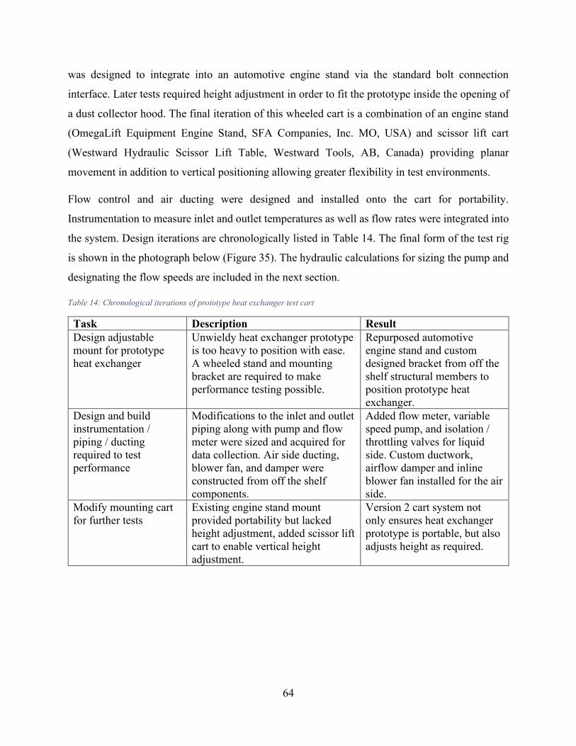
64

was designed to integrate into an automotive engine stand via the standard bolt connection

interface. Later tests required height adjustment in order to fit the prototype inside the opening of

a dust collector hood. The final iteration of this wheeled cart is a combination of an engine stand

(OmegaLift Equipment Engine Stand, SFA Companies, Inc. MO, USA) and scissor lift cart

(Westward Hydraulic Scissor Lift Table, Westward Tools, AB, Canada) providing planar

movement in addition to vertical positioning allowing greater flexibility in test environments.

Flow control and air ducting were designed and installed onto the cart for portability.

Instrumentation to measure inlet and outlet temperatures as well as flow rates were integrated into

the system. Design iterations are chronologically listed in Table 14. The final form of the test rig

is shown in the photograph below (Figure 35). The hydraulic calculations for sizing the pump and

designating the flow speeds are included in the next section.

Table 14: Chronological iterations of prototype heat exchanger test cart

Task Description Result

Design adjustable

mount for prototype

heat exchanger

Unwieldy heat exchanger prototype

is too heavy to position with ease.

A wheeled stand and mounting

bracket are required to make

performance testing possible.

Repurposed automotive

engine stand and custom

designed bracket from off the

shelf structural members to

position prototype heat

exchanger.

Design and build

instrumentation /

piping / ducting

required to test

performance

Modifications to the inlet and outlet

piping along with pump and flow

meter were sized and acquired for

data collection. Air side ducting,

blower fan, and damper were

constructed from off the shelf

components.

Added flow meter, variable

speed pump, and isolation /

throttling valves for liquid

side. Custom ductwork,

airflow damper and inline

blower fan installed for the air

side.

Modify mounting cart

for further tests

Existing engine stand mount

provided portability but lacked

height adjustment, added scissor lift

cart to enable vertical height

adjustment.

Version 2 cart system not

only ensures heat exchanger

prototype is portable, but also

adjusts height as required.

65

Figure 35: Final portable test cart for prototype heat exchanger

iii. Hydraulic system sizing and calculation The design of the fluid system follows the guidelines from McDonald and Magande’s book,

Introduction to Thermo-Fluids Systems Design, in order to get an estimated head requirement in

order to specify a pump suitable for the desired performance in the overall heat exchanger test

system [47]. All subsequently mentioned numerical limits, reference tables and figures in this

section are from the thermo-fluids design textbook unless otherwise stated.

Design notes:

• Heat exchanger tube ID is fixed at 0.87 inch

• Hard pipe sections connecting to heat exchanger flanges are fixed at 1.25-inch nominal diameter

66

o These sections are necessary because they fit onto the flanges of the prototype and they

include ports for submersion probe thermocouples

• Hose, pump, and flowmeters are available in the ½, ¾, 1, 1 ¼ inch diameters

o Lower diameter hose has reduced bend radius, i.e. more flexible

• Lower diameter flow meters are more sensitive to lower flow rates (2-10 GPM range)

• Assume flow splits equally from header pipe to each of the two loops, and as such, flow rate is

halved as illustrated in the following diagram:

Figure 36: Header pipe fluid distribution

• As per Table A.12 (adapted from 2005 Fundamentals, ASHRAE [48]), centrifugal pump suction

line flow velocity must be <4.9 ft/s [47]

o Use 4.9 ft/s as the maximum operating point

• Rubber hose roughness is similar or less than commercial steel pipe so Figure A.4 will be used for

calculations [47].

• A strainer will be installed on the supply side before the pump to protect the pump from any

particles which may be in the water as per guidelines [47]

• Isolation valves are used to isolate major hydraulic appurtenances such as the pump, flow meter,

as well as the heat exchanger [47]

• A water tank has been included in the design for portability, in the event that domestically supplied

water is not available in the test environment

o Water supply lines (domestic or tank) are assumed to have 0 head meaning the pump will

be required to supply all the work required to move the water through the system in order

to size the pump conservatively and not rely on supply side water pressure

67

• Ensure that flow rate is acceptable upon reaching the heat exchanger by staying below the 10 ft/s

erosion limit for carbon steel piping (Table A.13) [47]

• A throttling globe valve is included for fine flow rate control as per guidance [47]

Below is a sketch of the fluid system and will be used to perform the head loss calculations:

Figure 37: Fluid system - proposed design for pump sizing

The calculated minimum operating point is 7 GPM and 14.71 ft w.g. Calculations are shown in

section A.2. An adjustable circulator pump capable of exceeding this operating point was

selected. The Bell & Gossett ecocirc pump is able to supply a maximum head of 19 ft w.g. or

maximum flow rate of 16 GPM. The pump has a controller so the motor can be adjusted for

different operating points. The data sheet and pump curves for the pump are attached in section

A.4.

iv. Air flow control and measurement system design Tests were performed using domestic water supplies and air. An assortment of rigid and flexible

ducts and fittings were used as well as custom fabricated duct adapters to accommodate the 4-inch

diameter opening of a Tankless Water Heater (TWH) exhaust with the 17 by 17-inch cross section

of the prototype heat exchanger. Fluid control systems for both air and water were designed and

sourced from off the shelf components. An adjustable circulator pump which exceeded the

operating point requirements to avoid to the point design was selected (Bell & Gossett ecocirc®

19-16, Xylem Inc. NY, USA) and inline blower fan capable of up to 230 cfm airflow (Rule

Industries Model 240 4” Blower, Xylem Inc. NY, USA) were utilized for fluid flow control.

68

Dampers and throttling valves were sourced to provide finer adjustment for the air side and water

side.

A turbine flow meter (FTB792, Omega Engineering, Inc. QC, Canada) and Pitot tube measurement

kit (475-1-FM-AV Air Velocity Kit, Dwyer Instruments Inc. IN, USA) were used to measure the

flow rates of water and air, respectively. K-Type probe tip thermocouples with industrial protection

heads (NB1-CASS-14U-6, Omega Engineering, Inc. QC, Canada) measured water temperature at

ports near the inlet and outlet of the heat exchanger. Several J-Type thermocouples (GG-J-24,

Omega Engineering, Inc. QC, Canada) placed inside the ductwork were used to measure air

temperatures. A Keysight data acquisition (DAQ) / data logger switch unit (34970A, Keysight

Technologies, Inc. CA, USA) is used to record the various thermocouple outputs during the

experiments. The schematic below, Figure 38, shows the air and water side of the setup including

the appurtenances and instrumentations.

Figure 38: Schematic of testing setup for hot flue gas - cold water test

Before any tests were conducted, the system was assembled and pressurized with water. The

system is designed to be run as an open system other than a throttling valve to control the flow

rate, but as a measure of safety, the outlet valve was shut and the complete system was tested for

leaks. Over a duration of 30 minutes, a few drips were observed at threaded pipe interfaces, but

69

overall the system was not leaking in any major way. All NPT threaded joints were installed with

Teflon tape and inspected before testing.

A.2 Hydraulic design calculations for industrial-scale prototype Using Figure A.4, the choices of diameters for the hydraulic systems, and the max flow velocity

of 4.9 ft/s, we have the following operating points [47]:

Table 15: Operational flow rates and friction losses for various diameter hydraulic systems

Operating parameter Flow rate

(GPM)

Friction loss

(ft w.g. / 100

ft)

½ inch diameter, 4.9 ft/s 3.1 34

¾ inch diameter, 4.9 ft/s 7 22

1-inch diameter, 4.9 ft/s 13 15

1¼ inch diameter, 4.9 ft/s 19 13

It was necessary to ensure the flow rate is acceptable upon reaching the tubes inside the prototype

heat exchanger. For stainless steel pipes, this should be less than 15 ft/s from Table A.13 [47].

Since flow rate is halved at the heat exchanger after going from header to individual tube loops,

use the half of the highest flow rate case in the table above.

�̇� = 𝑉ave𝐴c

𝑉ave =�̇�

𝐴c

9.5 GPM (half of the 19 GPM maximum, as shown in the table above)

9.5 GPM =0.02117 ft3

s

𝑉ave =0.2117 ft3/s

𝜋[0.87 in ∙

1 ft12 in]

2

4

= 5.13 ft/s

Therefore, all 4 cases above are acceptable if the highest flow rate case is acceptable.

Calculate friction losses (in ft w.g.) to find pump head requirement. Calculations will be shown

for ¾ inch case:

Major Losses for ¾ inch, Q = 7 GPM (assuming fastest possible flow in pump suction piping)

70

Total length of pipe (excluding heat exchanger tubes), flow rates and corresponding friction losses

from Figure A.4 [47]:

2 × 26 inch hard pipe segments, 11

4 inch diameter @ 7 GPM flow rate →

1.75 ft w. g.

100 ft

3 × 5 foot hose segments, 3

4 inch diameter @ 7 GPM flow rate →

22 ft w. g.

100 ft

Major head loss equation is:

𝐻l,maj. = 𝐿1 (Head Loss in ft w. g.

100 ft for segment 1, at segment 1 flow rate)

+ 𝐿2 (Head Loss in ft w. g.

100 ft for segment 2, at segment 2 flow rate) + ⋯.

𝐻l,maj. = 4.33 ft (1.75 ft w. g.

100 ft) + 15 ft (

22 ft w. g.

100 ft)

𝐻l,maj. = 3.38 ft w. g.

Minor Losses

Using loss coefficients, K, on pipe fittings:

𝐻l,min. = ∑ 𝐾 ∙𝑉s

2

2𝑔

The following table is a compilation of the loss coefficients in the fluid system, some figures are

from component data sheets while most are from Table A.14 [47, p. 349].

Table 16: Loss coefficients for various hydraulic components

Component Loss Coefficient, K

Sharp edged entrance 0.5

Gate valve, screwed 0.3

Strainer 7.0

Flow meter 5.1

Globe valve 14.0

Ball valve 0.05

Expansion 0.15

90-degree elbow 2.0

Using the loss coefficients, the minor head losses are calculated:

71

𝐻l,min. = [∑ 𝐾34

inch section] ∙

(𝑉ave,

34

inch section)

2

2 (32.2 ft

s )+ [∑ 𝐾

114

inch section] ∙

(𝑉ave,1

14

inch section)

2

2 (32.2ft

s )

+ 𝐻l,heat exchanger

𝑉ave = 4.9ft

s at the

3

4 inch section

By conservation of mass, we can find the average flow velocity at the 1¼ inch section:

�̇� = 𝑉ave𝐴c = 4.9ft

s∙ 𝜋

[34 in ∙

1 ft12 in]

2

4= 𝑉

ave,114

inch section∙ 𝜋

[114 in ∙

1 ft12 in]

2

4

𝑉ave,1

14

inch section= 1.8 ft/s

Substituting known values:

𝐻l,min. = [2(0.30) + 0.5 + 0.05 + 7.0 + 5.1 + 14 + 0.15] ∙(

4.9fts )

2

2 (32.2ft

s )+ [2(2.0) + 2(0.05)]

∙(

1.8 fts )

2

2 (32.2 ft

s )+ 𝐻l,heat exchanger

𝐻l,min. = 10.215 + 0.206 + 𝐻l,heat exchanger

To calculate the head loss in the prototype heat exchanger, tracing the path of the water as it enters

one of the tubes in the heat exchanger:

𝐻l,heat exchanger = [𝑓𝑙heat exchanger tube

𝐷i+ ∑ 𝐾]

𝑉ave2

2𝑔

The following diagram shows the heat exchanger tube geometry from a top down view and the

loss coefficients associated with flow through one tube:

72

Figure 39: Heat Exchanger Single Tube Path Schematic

To find friction factor, f, using a Moody chart, the following values must be computed:

�̇� =7 GPM

2= 3.5 GPM = 0.0078

ft3

s

𝑉ave =0.0078

ft3

s

𝜋[0.87 in ∙

1 ft12 in]

2

4

= 1.89 ft/s

Take the density and viscosity of water at 145 degrees Fahrenheit (this temperature is chosen as

the estimated water temperature which would be travelling through the tubes during testing) and

calculate the Reynold’s number:

𝑅𝑒Di =𝜌𝑉𝐷i

𝜇=

61 lb/ft3(1.89 ft/s)(0.87 in ∙ 1 ft 12 in⁄ )

2.9 × 10−4 lb/(ft ∙ s)

Assume surface roughness of tubes is similar to commercial steel pipe as per Table A.1 [47, p.

339]:

휀

𝐷i=

0.046 mm

0.87 in ∙25.4 mm

in

= 0.0021

With the Reynold’s number and roughness ratio, we can find friction factor from a Moody Chart.

Reading from the chart, we get:

𝑓 = 0.029

Thus, we can calculate the head loss for the heat exchanger:

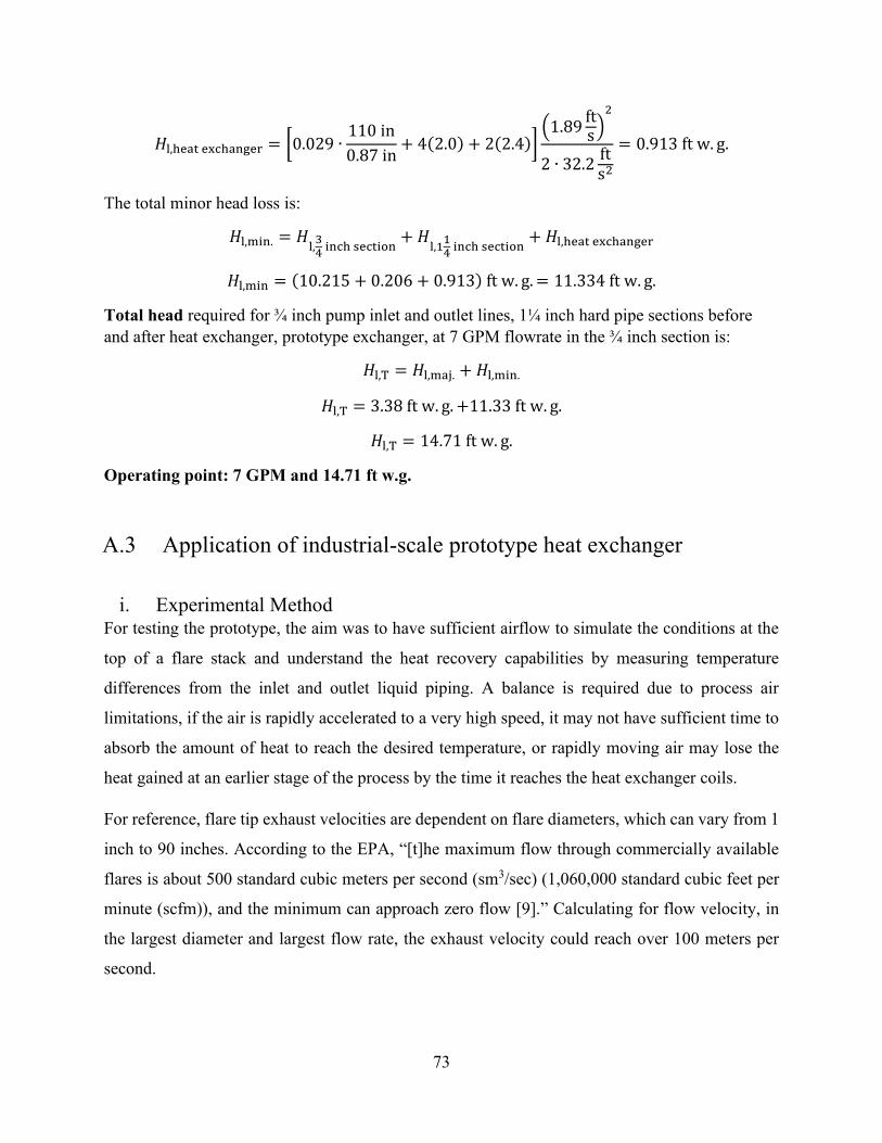
73

𝐻l,heat exchanger = [0.029 ∙110 in

0.87 in+ 4(2.0) + 2(2.4)]

(1.89fts)

2

2 ∙ 32.2fts2

= 0.913 ft w. g.

The total minor head loss is:

𝐻l,min. = 𝐻l,

34

inch section+ 𝐻

l,114

inch section+ 𝐻l,heat exchanger

𝐻l,min = (10.215 + 0.206 + 0.913) ft w. g. = 11.334 ft w. g.

Total head required for ¾ inch pump inlet and outlet lines, 1¼ inch hard pipe sections before

and after heat exchanger, prototype exchanger, at 7 GPM flowrate in the ¾ inch section is:

𝐻l,T = 𝐻l,maj. + 𝐻l,min.

𝐻l,T = 3.38 ft w. g. +11.33 ft w. g.

𝐻l,T = 14.71 ft w. g.

Operating point: 7 GPM and 14.71 ft w.g.

A.3 Application of industrial-scale prototype heat exchanger

i. Experimental Method For testing the prototype, the aim was to have sufficient airflow to simulate the conditions at the

top of a flare stack and understand the heat recovery capabilities by measuring temperature

differences from the inlet and outlet liquid piping. A balance is required due to process air

limitations, if the air is rapidly accelerated to a very high speed, it may not have sufficient time to

absorb the amount of heat to reach the desired temperature, or rapidly moving air may lose the

heat gained at an earlier stage of the process by the time it reaches the heat exchanger coils.

For reference, flare tip exhaust velocities are dependent on flare diameters, which can vary from 1

inch to 90 inches. According to the EPA, “[t]he maximum flow through commercially available

flares is about 500 standard cubic meters per second (sm3/sec) (1,060,000 standard cubic feet per

minute (scfm)), and the minimum can approach zero flow [9].” Calculating for flow velocity, in

the largest diameter and largest flow rate, the exhaust velocity could reach over 100 meters per

second.

74

For testing in air-to-water heat transfer configuration, the air temperature was required to be in

excess of 340 degrees Celsius upon reaching the heat exchanger and coil velocities should be above

5 meters per second. This temperature requirement is the minimum to begin exceeding previous

air-to-air tests [28]. Airflow velocity was problematic in prior testing because the velocity was too

low (≈1 meter per second) due to heater output limitations. The airflow velocity was too low to

reach the desired forced convection heat transfer regime and closer to a free convection

environment.

Flue gas heating domestic cold water

For the flue gas test, the prototype heat exchanger and engine stand combo were fitted with a duct

adapter to reduce the 17 by 17-inch square opening of the exchanger to a 4-inch round duct. As

part of the ductwork, the 230 cfm 4-inch inline blower fan was installed to pull air onto the heat

exchanger coils along with a flow control damper. A 4-inch round duct is the size which fit over

the flue gas outlet of a natural gas burning, Rinnai tankless water heater (TWH) unit (Rinnai V75i,

Rinnai America Corporation, GA, USA). This TWH unit flue exhaust can reach temperatures of

300 degrees Fahrenheit and was the first available candidate to generate hot exhaust flue gasses

for testing the prototype heat exchanger as it was available for use from a previous research project.

Figure 40 is a photograph of the test setup and instrumentation.

During the tests, the TWH was run with the hottest setting and continuous flow of cool water. In

this operating condition, the TWH was constantly operating at the highest burner setting in order

to generate the hottest flue gasses. Two sets of three thermocouples were used, one set placed near

the flue gas outlet and another set near the heat exchanger tubes to measure the temperature drop

of the flue gas. The flow rate of water through the heat exchanger was initially kept as low as

possible to decrease the flow velocity and increase the heating time. The fan ran at full speed and

the damper was fully open to draw as much hot air as possible onto the heat exchanger tube

surfaces.

75

Figure 40: Photograph of hot flue gas - cold water test setup

Flame impingement heating passes

In order to increase temperature on the heat exchanger tubes, another approach was attempted. A

flame spray torch (6P-II, Oerlikon Metco AG, ZH, Switzerland) attached to a robotic manipulator

(HP20, Motoman, Mississauga, ON, Canada) was used for direct flame impingement passes over

the heat exchanger tubes. To operate the system safely, the prototype heat exchanger was placed

in front of the thermal spray hood with the ventilation system running. This ensures any

combustion or incomplete combustion gases were safely exhausted from the lab.

The robotic manipulator arm was programmed to move at the highest possible speed, traversing

over the cross-section area to provide even heating. A schematic of the final traverse pattern is

shown below in Figure 41. The red dots represent the points which were “taught” to the robot

during programming. White arrows approximate the linear trajectory that the torch tip followed.

The linear traverse speed of the robot was set to the maximum allowable, 1500 mm per second.

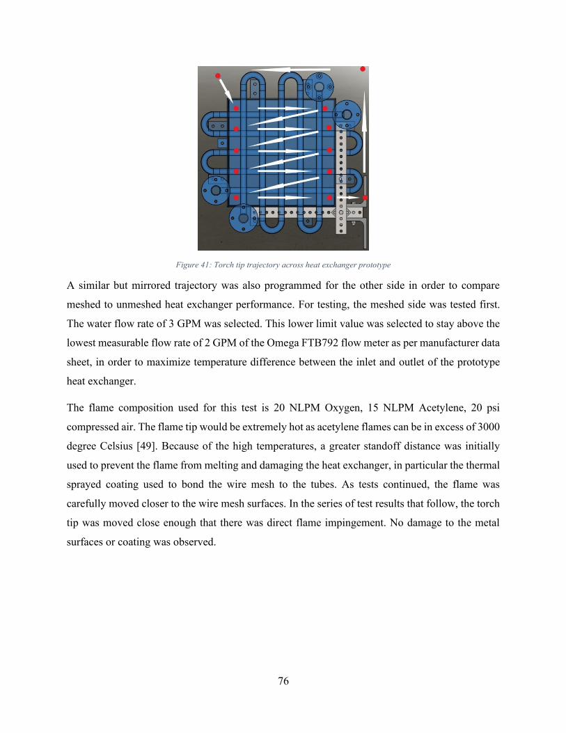
76

Figure 41: Torch tip trajectory across heat exchanger prototype

A similar but mirrored trajectory was also programmed for the other side in order to compare

meshed to unmeshed heat exchanger performance. For testing, the meshed side was tested first.

The water flow rate of 3 GPM was selected. This lower limit value was selected to stay above the

lowest measurable flow rate of 2 GPM of the Omega FTB792 flow meter as per manufacturer data

sheet, in order to maximize temperature difference between the inlet and outlet of the prototype

heat exchanger.

The flame composition used for this test is 20 NLPM Oxygen, 15 NLPM Acetylene, 20 psi

compressed air. The flame tip would be extremely hot as acetylene flames can be in excess of 3000

degree Celsius [49]. Because of the high temperatures, a greater standoff distance was initially

used to prevent the flame from melting and damaging the heat exchanger, in particular the thermal

sprayed coating used to bond the wire mesh to the tubes. As tests continued, the flame was

carefully moved closer to the wire mesh surfaces. In the series of test results that follow, the torch

tip was moved close enough that there was direct flame impingement. No damage to the metal

surfaces or coating was observed.

77

Figure 42: Flame used for heating passes

Air cooling heated water from TWH

A reversal of heat transfer direction was explored in the final test setup. The outlet heated water of

the TWH was fed into the inlet piping of the heat exchanger. A large vane axial fan which roughly

covers the 17 by 17-inch square cross section of the heat exchanger was placed in front of the

prototype heat exchanger coils and ambient air was blown over the tubes to cool the water flowing

inside. The flue gas exhaust from the TWH was directed into the thermal spray hood allowing the

ventilation system to remove the flue or natural gas from incomplete combustion. A photo of the

setup is shown below.

78

Fan Specification:

- 24” impeller diameter

- 1140 RPM

- 0.54 HP

- Woods Fans (Canada) Limited

Measured air pressure:

- 0.18 to 0.22 in wc

- Dwyer Pitot tube

- Approx. 1800 to 2000 fpm

- Air flow was non-uniform

Ambient air temperature:

- 23 degrees C

Measured maximum water

temperature (TWH outlet):

- 44 degrees C

Prototype heat exchanger test

loop:

- Meshed tube loop

Sampling frequency:

- 1 Hz

Again, the test was run with the meshed tube rows first, to see if an appreciable temperature

difference between inlet and outlet is measurable. If not, no bare tube tests will be conducted as

the performance comparison is not possible without significant temperature differences. The

Keysight data logger was set to record the temperature every second. The water flowrate was tested

at three set points of 4, 6 and 8 GPM using the throttling valve. The fan was a single speed unit. A

pitot tube was used to measure the airflow velocity of the vane axial fan.

ii. Results and Discussion

Flue gas heating domestic cold water

In total, three water flow rates were tested. At each water flow rate set point, the system ran

continuously for 15 minutes to ensure steady state, measurements were taken when the outlet water

temperature was no longer rising. The result of the flue gas test is as follows:

Figure 43: Large vane axial fan for air cooling tests

79

Table 17: Flue gas heat exchanger test results for three water flow rates

Inlet air

temperature

[℃]

Water

flow rate

[GPM]

Inlet water

temperature

[℃]

Outlet

water

temperature

[℃]

Temperature

difference

[℃]

115.5 3.03 11.7 14.7 3.0

117.0 5.07 11.7 13.0 1.3

118.0 7.01 11.7 12.6 0.9

An NTU-based calculator software was used to compared predicted results with actual results. The

software, COIL – Plate-Fin-Tube Coil Analyzer, was used for predicting coil performance is

bundled with the McQuiston HVAC Analysis & Design textbook [50]. Detailed inputs and outputs

for modelling the flue gas heating tests are included in section A.5.

For the entering and leaving fluid temperatures, the simulated temperature difference is 2.7 degrees

Fahrenheit (1.5 degrees Celsius) falling in line with the experimental result temperature difference

as listed in Table 17. The flow rate in the calculation was higher than experimentally achieved

(12.2 GPM) so the calculated performance was slightly better than experimentally achieved

results. Thus, for the test case, with the flue gas from the TWH, an industry standard plate-fin tube

exchanger may perform better than the mesh-based prototype.

Since the overall fluid temperature difference is quite low, the results of the test and similar

simulated result indicate that the flue gas temperature was insufficient to change the water

temperature in a significant manner. Various factors affected the amount of heat transferred:

• The water flow rate was near the minimum as the flow meter required at minimum 2 GPM

• The duct system lost heat (~20-25 degrees Celsius) from the TWH to the air inlet on the heat

exchanger (TWH flue gas exhaust was around 140 degrees Celsius, close to the 300-degree

Fahrenheit figure as the manufacturer had specified)

• Ducting losses are difficult to mitigate because the duct is already as short as possible given the lab

spacing and configuration of the test equipment

• Airflow is too low due to the large expansion from 4-inch round to 17-inch square, the low volume

flow rate flue gas exhaust from the TWH results in an even lower average flow velocity upon

reaching the expanding duct adapter, at the duct expansion, flue gasses also cool rapidly

80

Result: In order to increase temperature difference between the water inlet and outlet of the heat

exchanger requires increased coil velocities and temperatures.

Flame impingement heating passes

The time to reach steady state temperatures was unknown. As such, tests were run for over 500

seconds to allow sufficient time for the system to reach steady state. Two tests were run to see if

the high (1500 mm/s) and low (500 mm/s) trajectory speed would cause a noticeable difference in

temperature rise. The inlet and outlet water temperature are logged for the duration of the test at

every 5 seconds with the Keysight DAQ and are shown in the plots below. The logging will show

if a steady temperature difference is achieved and when the temperature difference reaches steady

state, if at all.

Figure 44: 500 mm/s robot speed flame spray heating

Figure 45: 1500 mm/s robot speed flame spray heating

Again, similar to the flue gas heating test, the results of the flame impingement test indicate that

the flame impingement passes over the heat exchanger mesh and tube were insufficient to change

the water temperature in a significant manner, although as expected, the outlet temperature was

0

5

10

15

20

0 100 200 300 400 500 600Tem

per

atu

re (

deg

. C)

Time Elapsed (sec.)

Inlet Temp

Outlet Temp

0

5

10

15

20

0 200 400 600 800 1000 1200

Tem

per

atu

re (

deg

. C)

Time Elapsed (sec.)

Inlet Temp

Outlet Temp

81

slightly higher than at the inlet. The increased flame spray torch tip traverse speed did not produce

a noticeable increase in outlet temperature.

The meshed side tests showed that inlet / outlet temperature difference stayed the same at 1 or 2

degrees Celsius. The overall temperature fluctuation of the domestic water supply had more effect

on the temperature measurement than the heating due to flame impingement. As such, the

unmeshed tube loops were not tested, the comparison between the meshed and unmeshed tubes is

not measurable at these minimal temperature differences. Various factors impacted the amount of

heat transferred:

• To maximize water temperature difference, the water flow rate was near the minimum (flow meter

required at minimum 2 GPM for accurate measurements)

• The flame impingement was only onto the first layer of the multi layered heat exchanger, meaning

the tube loop deeper inside was not heated as much as the outermost tube and was mixing the colder

water contained inside it with the heated tube loop once reaching the header before the outlet,

ultimately reducing outlet temperature

• Heat was essentially a point source, and despite the very hot point moving across the whole cross

section, there was not enough heat being transferred from the flame across the complete heat

exchanger cross section, areas were cooling down before the flame had a chance to pass over again

• A larger flame or torch array could be considered to cover more of the cross section and reduce the

need to traverse the flame over the cross section


exchanger, the system requires increased simultaneous heat transfer across the whole cross section

area. A single, very high temperature point source is not sufficient even if moved over the cross-

section area at high speeds.

Air cooling heated water from TWH

The inlet and outlet water temperatures of the TWH supplied domestic hot water cooled by ambient

room temperature air is logged for over 10 minutes at three flow rates. The plots of the

temperatures are shown in the figures below.

82

Figure 46: 4.02 GPM cool air test temperature log



The approximately 0.5-degree Celsius temperature difference in the two higher flow rate tests are

too insignificant and could be a result of thermocouple discrepancy (systematic error). As can be

seen over the majority of the 10-minute tests, the temperature difference remains unchanged. The

parallel nature of the inlet and outlet temperature plots indicates that the fluctuations are caused

by temperature changes at the source (TWH) and not by airflow cooling the water through

convection heat transfer. Thus, at the two high flowrate test cases (6.85 and 8.14 GPM), the heat

exchanger cooling performance is not measurable.

43

43.5

44

44.5

45

0 100 200 300 400 500 600 700Tem

per

atu

re (

Cel

ciu

s)

Time (Seconds)

Inlet

Outlet

43

43.5

44

44.5

45

45.5

0 100 200 300 400 500 600 700 800 900 1000

Tem

per

atu

re (

Cel

ciu

s)

Time (Seconds)

Inlet

Outlet

42

42.5

43

43.5

44

44.5

0 100 200 300 400 500 600 700Tem

per

atu

re (

Cel

ciu

s)

Time (Seconds)

Inlet

Outlet

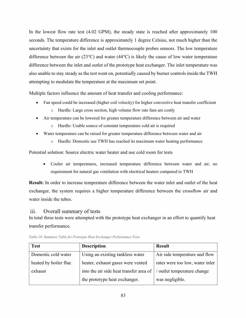
83

In the lowest flow rate test (4.02 GPM), the steady state is reached after approximately 100

seconds. The temperature difference is approximately 1 degree Celsius, not much higher than the

uncertainty that exists for the inlet and outlet thermocouple probes sensors. The low temperature

difference between the air (23℃) and water (44℃) is likely the cause of low water temperature

difference between the inlet and outlet of the prototype heat exchanger. The inlet temperature was

also unable to stay steady as the test went on, potentially caused by burner controls inside the TWH

attempting to modulate the temperature at the maximum set point.

Multiple factors influence the amount of heat transfer and cooling performance:

• Fan speed could be increased (higher coil velocity) for higher convective heat transfer coefficient

o Hurdle: Large cross section, high volume flow rate fans are costly

• Air temperature can be lowered for greater temperature difference between air and water

o Hurdle: Usable source of constant temperature cold air is required

• Water temperature can be raised for greater temperature difference between water and air

o Hurdle: Domestic use TWH has reached its maximum water heating performance

Potential solution: Source electric water heater and use cold room for tests

• Cooler air temperatures, increased temperature difference between water and air, no

requirement for natural gas ventilation with electrical heaters compared to TWH


exchanger, the system requires a higher temperature difference between the crossflow air and

water inside the tubes.

iii. Overall summary of tests In total three tests were attempted with the prototype heat exchanger in an effort to quantify heat

transfer performance.

Table 18: Summary Table for Prototype Heat Exchanger Performance Tests

Test Description Result

Domestic cold water

heated by boiler flue

exhaust

Using an existing tankless water

heater, exhaust gases were vented

into the air side heat transfer area of

the prototype heat exchanger.

Air side temperature and flow

rates were too low, water inlet

/ outlet temperature change

was negligible.

84

Domestic cold water

heated by flame

impingement

A robotic manipulator with a flame

spray torch traverses rapidly over

the air side cross section area to

heat up water flowing inside the

tubes.

Heat imparted over the tube

and mesh cross section was

insufficient to change water

temperature by more than

3˚C.

Heated water cooled by

ambient air

Using a large vane axial fan, room

temperature air was blown over the

cross-section area to cool heated

water flowing inside the tubes.

Temperature difference

between air (21˚C) and water

(44˚C) was too small to cool

water by more than 2˚C.

All tests had elements which were improvements but also insufficiencies. For the first test, both

air side flow rates and temperatures were not high enough. The second test improved on the air

side temperatures, but area of effect was not large enough. The third test provided sufficient

airflow, but temperature difference was insufficient. From the various tests performed with the

prototype, each test showed both areas of improvement leading to a redesigned heat exchanger and

compatible test setup which was fabricated in an effort to continue development of novel thermally

sprayed tubular heat exchangers. It was important to design the samples alongside the test

apparatus so aforementioned testing challenges could be avoided and capabilities of the test system

would be sufficient to heat the samples. The following sections apply the aforementioned learnings

leading to a modified approach to continue development of thermal sprayed mesh tubular heat

exchangers.

85

A.4 Circulator pump performance curves

A.5 Simulated results of flue gas prototype heat exchanger tests COIL – Plate-Fin-Tube Coil Analyzer was used to give comparable performance of industry

standard plate-fin tube exchangers [51].

86

Figure 49: Main screen of Coil program graphical user interface

The following screenshot outlines the inputs to the program. Care was taken to get a close

approximation to the prototype heat exchanger as possible with the assumption that a similar sized

plate-fin tube would perform in the same order of magnitude as the novel mesh tube prototype. As

previously stated, the fin / tube materials are stainless steel, the dimensions are 17”, there are 2

tube rows with 5 tubes per row. These measurements are specified to reflect the dimensions to the

prototype heat exchanger. Because wire meshes are used instead of fins, the fin pitch is spaced in

the same dimensions that the mesh sheets are spaced. Fin thickness was taken to be wire thickness

of the wire that is weaved to form the mesh. Dry bulb temperature and face velocity were chosen

in accordance to the best estimates from the TWH outlet temperature measurement and duct blower

fan specifications.

87

Figure 50: Input for calculating TWH flue gas heating scheme for prototype heat exchanger

Results of the calculation program were outputted in the following window:

Figure 51: Output results of simulated prototype heat exchanger

88

Appendix B

B.1 Drawings for tube bending, tube press, and assembly process

development of thermal sprayed tube and mesh heat

Documents