dfg funded project gepavas project report - uni-duesseldorf.de · dfg funded project gepavas...
TRANSCRIPT

DFG funded ProjectGepavas
(Gerichtete und Parallele Verifikation von abstrakten Spezifikationen)
Project ReportWork Conducted Until June 2010
Jens Bendisposto, Markus Borgermans, Michael Leuschel
Institut fur Informatik, Universitat DusseldorfUniversitatsstr. 1, D-40225 Dusseldorf
{ bendisposto, leuschel } @cs.uni-duesseldorf.de

Table of Contents
DFG funded Project Gepavas (Gerichtete und Parallele Verifikation von ab-
strakten Spezifikationen) Project Report Work Conducted Until June 2010 . . . 1Jens Bendisposto, Markus Borgermans, Michael Leuschel
1 Management Summary . . . . . . . . . . . . . . . . . . . . . . . . . . . . . . . . . . . . . . . . . . 31.1 Overview . . . . . . . . . . . . . . . . . . . . . . . . . . . . . . . . . . . . . . . . . . . . . . . . . . 31.2 Published papers and presentations . . . . . . . . . . . . . . . . . . . . . . . . . . . 31.3 Outlook . . . . . . . . . . . . . . . . . . . . . . . . . . . . . . . . . . . . . . . . . . . . . . . . . . . 3
2 Workpackage T1: Case Studies . . . . . . . . . . . . . . . . . . . . . . . . . . . . . . . . . . . . 52.1 Overview of Case Studies . . . . . . . . . . . . . . . . . . . . . . . . . . . . . . . . . . . . 52.2 Models with Invariant Violations . . . . . . . . . . . . . . . . . . . . . . . . . . . . . 52.3 Models with Deadlocks . . . . . . . . . . . . . . . . . . . . . . . . . . . . . . . . . . . . . . 62.4 Models with GOAL to be found . . . . . . . . . . . . . . . . . . . . . . . . . . . . . . 72.5 Models without Errors . . . . . . . . . . . . . . . . . . . . . . . . . . . . . . . . . . . . . . 82.6 Tool developments . . . . . . . . . . . . . . . . . . . . . . . . . . . . . . . . . . . . . . . . . . 10
3 Workpackage E1: Empirical Evaluation . . . . . . . . . . . . . . . . . . . . . . . . . . . . 113.1 Initial Motivation: Model Checking High-level versus Low-level
Specifications . . . . . . . . . . . . . . . . . . . . . . . . . . . . . . . . . . . . . . . . . . . . . . 113.2 A small empirical study . . . . . . . . . . . . . . . . . . . . . . . . . . . . . . . . . . . . . 113.3 Looking for Answers . . . . . . . . . . . . . . . . . . . . . . . . . . . . . . . . . . . . . . . . 123.4 Depth-First versus Breadth-First: A thorough empirical Evaluation 143.5 Evaluation the potential of using Heuristics . . . . . . . . . . . . . . . . . . . . 163.6 Overall Conclusions of all Experiments . . . . . . . . . . . . . . . . . . . . . . . . 203.7 Experimental Results (Figures and Tables) . . . . . . . . . . . . . . . . . . . . 20
4 Workpackage I1: Generic Parallelisation Prototype . . . . . . . . . . . . . . . . . . 304.1 Interfacing with SICStus Prolog . . . . . . . . . . . . . . . . . . . . . . . . . . . . . . 304.2 Share data using the SICStus C-Interface . . . . . . . . . . . . . . . . . . . . . . 304.3 Using ProB with shared memory . . . . . . . . . . . . . . . . . . . . . . . . . . . . . 324.4 Using Berkely DB . . . . . . . . . . . . . . . . . . . . . . . . . . . . . . . . . . . . . . . . . . 324.5 Combining ProB and Spin . . . . . . . . . . . . . . . . . . . . . . . . . . . . . . . . . . 324.6 Future Work . . . . . . . . . . . . . . . . . . . . . . . . . . . . . . . . . . . . . . . . . . . . . . . 32
5 Workpackages T2/I2: Abstract Interpretation of B . . . . . . . . . . . . . . . . . . 345.1 Predicate Analysis . . . . . . . . . . . . . . . . . . . . . . . . . . . . . . . . . . . . . . . . . . 345.2 Generic Abstract Interpretation Framework for B. . . . . . . . . . . . . . . 355.3 Flow Analysis for B . . . . . . . . . . . . . . . . . . . . . . . . . . . . . . . . . . . . . . . . 36
6 Workpackage T3: Intelligent Techniques for Directed and Parallel ModelChecking . . . . . . . . . . . . . . . . . . . . . . . . . . . . . . . . . . . . . . . . . . . . . . . . . . . . . . 376.1 Proof supported and proof-directed model checking . . . . . . . . . . . . . 386.2 Automatic Flow Analysis . . . . . . . . . . . . . . . . . . . . . . . . . . . . . . . . . . . . 49
7 Workpackage I3: Parallel and Directed ProB. . . . . . . . . . . . . . . . . . . . . . . . 647.1 Implementation and Evaluation of Proof-Directed MC . . . . . . . . . . 657.2 Experimental results . . . . . . . . . . . . . . . . . . . . . . . . . . . . . . . . . . . . . . . . 65

1 Management Summary
1.1 Overview
Workpackages T1 (case studies), E1 (empirical evaluation) have been completed.A directed model checking algorithm has been implemented and empiricallyevaluated. Parts of workpackage T3 and to some extend also I3 have been startedmuch earlier than planned, and have already generated a scientific paper. Indeed,two avenues of research have been identified as particularly promising: proof-directed model checking and flow-analysis guided model checking. This explainsthat more resources were put into pursuing these avenues. This shift of focus hasbeen triggered by the further emergence of Event-B and the Rodin platform,where a model checker has direct access to proof obligations and the variousprovers.
Workpackage I1 (parallel prototype) is nearing completion. However, due tothe rising availability of multi-core systems, we have concentrated our efforts ona shared memory approach. Other approaches will be investigated in the nextphase of the project. The project is thus progressing very well.
1.2 Published papers and presentations
The following papers have been published within the project:
– Michael Leuschel, The High Road to Formal Validation, Proceedings ABZ2008, LNCS 5238, p. 4–23.
– Jens Bendisposto, Michael Leuschel: Proof Assisted Model Checking for B,Proceedings ICFEM 2009, LNCS 5885 , p. 504–520.
– Jens Bendisposto and Michael Leuschel. Parallel Model Checking of Event-BSpecifications with ProB. Preliminary Proceedings PDMC 2009, Eindhoven,November 2009.
– Mireille Samia, Harald Wiegard, Jens Bendisposto, Michael Leuschel : High-Level versus Low-Level Specifications: Comparing B with Promela and ProBwith Spin, Proceedings TFM-B 2009, Nantes, June, 2009, APCB.ISBN:2951246102.
In addition, two papers have been submitted for publication “Automatic FlowAnalysis for Event-B” and “Directed Model Checking for B: An Evaluation andNew Techniques”.
1.3 Outlook
The outcome of the empirical evaluation is that we believe that proof-directedand flow-analysis-directed model checking to be the most promising avenues forfurther work. We believe that a genetic library is less likely to yield good results.1
1 In the project description we promised we would evaluate whether this approach islikely to be fruitful or not.

On the other hand, an avenue that we had discarded in the original descriptionnow seems more more likely to be fruitful: (dynamic) partial order reduction.This change is again triggered by the rise of Event-B, which with its simplerevents, provides a much better basis for partial order reduction. Furthermore,Event-B has been designed for modelling reactive systems, and as such there isa much bigger need but also potential for partial order reduction.
Hence, in phase two of the project we plan to:
– pursue proof- and flow-analysis-directed model checking much more con-cretely, and
– develop and experiment with (dynamic) partial order reduction techniquesfor Event-B.

2 Workpackage T1: Case Studies
2.1 Overview of Case Studies
We have chosen a variety of case studies for evaluating the effectiveness of exist-ing and new techniques for model checking, in particular directed and parallelmodel checking. All models are either classical B models or Rodin Event-B mod-els. We have included several industrial specifications (some stemming from vari-ous EU projects, such as Rodin and Deploy2), as well as academic specificationsof various intricate algorithms. There are a few artificial benchmarks as well,testing specific aspects of the model checking algorithm. We have also includedsome classical puzzles as well, in particular to test directed model checking.
The case studies have been partitioned into four classes:
1. Models with invariant violations,2. Models with deadlocks,3. Models with no errors (i.e., no deadlocks or invariant violations), but where
a particular GOAL predicate is to be found. Indeed, in ProB the user candefine a particular GOAL predicate and ask the model checker to find stateswhich make the predicate true. The main difference with point 1 is that thegoals are often much more precise (sometimes a concrete particular state)than the invariant violations.
4. Models with no errors, and where the full state space needs to be explored.
Below we briefly describe the individual models. They are used extensively inthe empirical evaluation E1 (Section 3), as well as in the later tasks of the project.Note that new models will be added as the project progresses. We then describein subsection 2.6 tool developments that we have made, so that the performanceof a particular model checking technique can be automatically evaluated for allthose models.
2.2 Models with Invariant Violations
– Scheduler errThe process scheduler from [34] for 5 processes, where an error has beenadded to the model.
– Simpson Four SlotA model of Simpson’s four slot algorithm. This B model only represents theindividual steps of the algorithm. It is intended to be used in conjunctionwith a CSP model to describe the sequencing of the steps. Here, the B modelon its own is model checked (thus leading to invariant violations).
– TravelAgencyA B model of a distributed online travel agency, through which users canmake hotel and car rental bookings. It consists of 6 pages of B and wasdeveloped within the ABCD3 project.
2 EU funded FP7 research project 214158: DEPLOY (Industrial deployment of ad-vanced system engineering methods for high productivity and dependability).
3 “Automated validation of Business Critical systems using Component-based Design,”EPSRC grant GR/M91013.

– Peterson errPeterson is the specification of the mutual exclusion protocol for n processesas defined in [47]. Here we have used 4 processes and have introduced anerror in the protocol.
– SecureBuildingThe model of a secure building equipped with access control; see [?].
– NastyVendingMachineThe model of a simple ticket vending machine. Note that we have comparedthe performance of ProB with Spin in [35] (also in Appendix ?).
– Alstom axl3A train model by Alstom (confidential). This is not the final model but anintermediate one which still contains errors.
– dfcheck housesetA simple model (derived from Schneider’s houseset example [51]), where anoperation can add new house numbers to a set. An invariant violation occurswhen the set exceeds a certain limit.
– BreadthFirstTest, DepthFirstTest , DepthFirstTest2 Three artificialmodels, to test certain performance aspects of depth-first and breadth-firstsearch.
– Abrial Press m2 errA larger development of a mechanical by press by Abrial [2]. The develop-ment of the mechanical press started from a very abstract model and wentthrough several refinements. The final model contained “about 20 sensors,3 actuators, 5 clocks, 7 buttons, 3 operating devices, 5 operating modes,7 emergency situations, etc.” [2]. This model is a variation of the secondrefinement, where an error has been introduced.
– SAP M PartnerAn Event-B model of a business process generated by SAP from a MCMchoreography model. This model describes the behaviour of an individualpartner. See [56].
– Needham-SchroederThe Needham-Schroeder public key protocol is an authentication protocol forcreating a secure connection over a public network [44]. The model consistsof a network with the two normal users called Alice and Bob, an attackernamed Eve and the keyserver. The first version of this protocol, developedin 1978, contains an error which was found in 1995 [41].This model is a slightly simplified version (reducing the messages sent byEve), to allow the model checker to more quickly find a counter example.The shortest counter example has 14 steps.
2.3 Models with Deadlocks
– Abrial Earley 3 v3, Abrial Earley 3 v5, Abrial Earley 4 v3A model developed by Jean-Raymond Abrial, with the help of DominiqueCansell. The purpose was to formally derive the Earley parsing algorithm in

Event-B and to establish its correctness. The model contains four levels of re-finement and very complicated guards. Every event corresponds to a step inthe parsing algorithm. The purpose was to animate the model for a particulargrammar and to reproduce the sequence in http://en.wikipedia.org/wiki/Earley parser.However, ProB did locate deadlocks (in fully proven models). For more de-tails see [11].
– Alstom axl3 deadlockThe same model as above; but this time we only look for deadlocks.
– Alstom exemple7Another model by Alstom (confidential). This is again not the final modelbut an intermediate one which still contains errors. One counter exampletrace has length 22.
– Bosch CrsCtrlThe second level of refinement of a Bosch model of an adaptive cruise controlsystem, developed within Deploy.
– SAP MChoreographyAn Event-B model of a business process generated by SAP from a MCMchoreography model. This model describes the behaviour of an global system.See [56].
– DiningThe classical Dining philosophers problem, with 8 philisophers.
– CXCC0CXCC (Cooperative Crosslayer Congestion Control) [50] is a cross-layerapproach to prevent congestion in wireless networks. The key concept isthat, for each end-to-end connection, an intermediate node may only for-ward a packet towards the destination after its successor along the route hasforwarded the previous one. The information that the successor node hassuccessfully retrieved a package is gained by active listening. The model isdescribed in [10]. The invariants used in the model are rather complex.
2.4 Models with GOAL to be found
– WegenetzThe problem is to find a target state within a graph. The shortest solutionneeds 14 moves.
– RussianPostalPuzzleThis is a B model of a cryptographic puzzle. (see, e.g., [23]). The shortestsolution needs 10 moves.
– TrainTorchPuzzleThe shortest solution needs 7 moves.
– BlocksWorldA model of blocksworld, with five blocks; the goal being to put all blocks inthe right-order on top of each other. The shortest solution needs 6 moves.
– FarmerThe Farmer/Fox/Goose/Grain puzzle. The shortest solution needs 9 moves.

– HanoiThe well-known towers of Hanoi puzzle. The shortest solution needs 33moves.
– Puzzle8The well-known eight puzzle.4 The goal is to arrive at a configuration wherethe eight tiles are in the correct order. The shortest solution needs 17 moves.
– RushHourThe Rush Hour puzzle.5 This is the hardest puzzle (number 40 in the regularversion of the game). The shortest solution needs 83 moves.
– Abrial Press m13This is the last level of refinement of [2]; already described above. The goalis the guard of a partcular event (traiter arret moteur 2).The shortest solution has length 3.
– Abrial Queue m1Level 1 of a non-blocking concurrent Queue algorithm, derived by Abrialand Cansell in [4]. The goal is to find a particular configuration of the datas-tructures of the algorithm(#pp.(pp:PROCESS & pp:dom(tld) & tld(pp)=hdd(pp) & tld(pp)=Tail))).The shortest solution has length 4.
– SystemOnChip RouterA system-on-chip router developed by Satpathy. The shortest solution haslength 4.
2.5 Models without Errors
– Scheduler1Another version of the process scheduler, for 5 processes. The first level ofrefinement from [37].
– Volvo CruiseVolvo Vehicle Function. The B specification machine has 15 variables, 550lines of B specification, and 26 operations. The invariant consists of 40 con-juncts. This B specification was developed by Volvo as part of the EuropeanCommission IST Project PUSSEE (IST-2000-30103).
– USB4USB is a specification of a USB protocol, developed by the French companyClearSy.
– Nokia NotaA model developed by Nokia within the RODIN Project6 for the validationand verification of Nokia’s NoTA hardware platform; see [45].
– HuffmanM Event-B model of a Huffman encoder/decoder.– Cansell Contention
A Firewire-Leader election protocol by Dominique Cansell, see also [48].
4 See, e.g., http://en.wikipedia.org/wiki/Fifteen puzzle.5 See http://en.wikipedia.org/wiki/Rush Hour (board game).6 http://rodin.cs.ncl.ac.uk/

– DeMoney GS R1 Part of a model of an electronic purse by Trusted Logic,developed within the SecSafe project. See for example [12].
– SystemOnChip Router1See above, but not searching for goal.
– Mondex m2, Mondex m3The mechanical verification of the Mondex Electronic Purse was proposedfor the repository of the verification grand challenge in 2006. We use anEvent-B model developed at the University of Southampton [17]. We havechosen two refinements from the model, m2 and m3. The refinement m2 isa rather big development step while the second refinement m3 was used toprove convergence of some events introduced in m2, in particular, m3 onlycontains gluing invariants.
– Siemens ATP0This Siemens Mini Pilot was developed within the Deploy Project. It isa specification of a fault-tolerant automatic train protection system, thatensures that only one train is allowed on a part of a track at a time. Themodel contains a single refinement level and rather complex invariants.
– SSF obsw1The Space Systems Finland example is a model of a subsystem used forthe ESA BepiColombo mission. The BepiColombo spacecraft will start in2013 on its journey to Mercury. The model is a specification of parts of theBepiColombo On-Board software, that contains a core software and two sub-systems used for tele command and telemetry of the scientific experiments,the Solar Intensity X-ray and particle Spectrometer (SIXS) and the Mer-cury Imaging X-ray Spectrometer (MIXS). The model was a mini pilot ofthe Deploy project.
– ETH elevator12This is the twelfth revienement of an elevator model by ETH Zurich.
– EchoThe Echo algorithm [19] is designed to find the shortest paths in a net-work topology. A start node sends an explore-message to all neighbors. Eachnode is marked with red, when it receives an explore-message for the firsttime. Moreover, it memorizes the nodes, from which it received the mes-sage, as a shortest path to the initialization node. It also sends, in turn,explore-messages to its other neighbors. Whenever the node receives eitheran explore-message or an echo-message from all its neighbors, to which itsent one of such messages, the node will be marked green and sends an echo-message to the nodes, from which it had first received an explore-message.When all nodes are marked green, the cycle is finished.In the B model, every type of message type has one corresponding operation.The operations are active, as soon as a node sends the appropriate message.The execution of the operation reflects the receipt of the message by thenode’s recipient. By the non-deterministic order, the selection of the activeoperations is assured that any various long message runtime in the channelof the model is taken into account. It is possible that many messages aresimultaneously on the channel. The edges are depicted as functions between
the nodes. With the proper invariants, it is easy to verify if a protocol ensuresthat all nodes are marked green, when no message is in the channel. Fur-thermore, all shortest paths must be known as soon as all nodes are markedgreen.
2.6 Tool developments
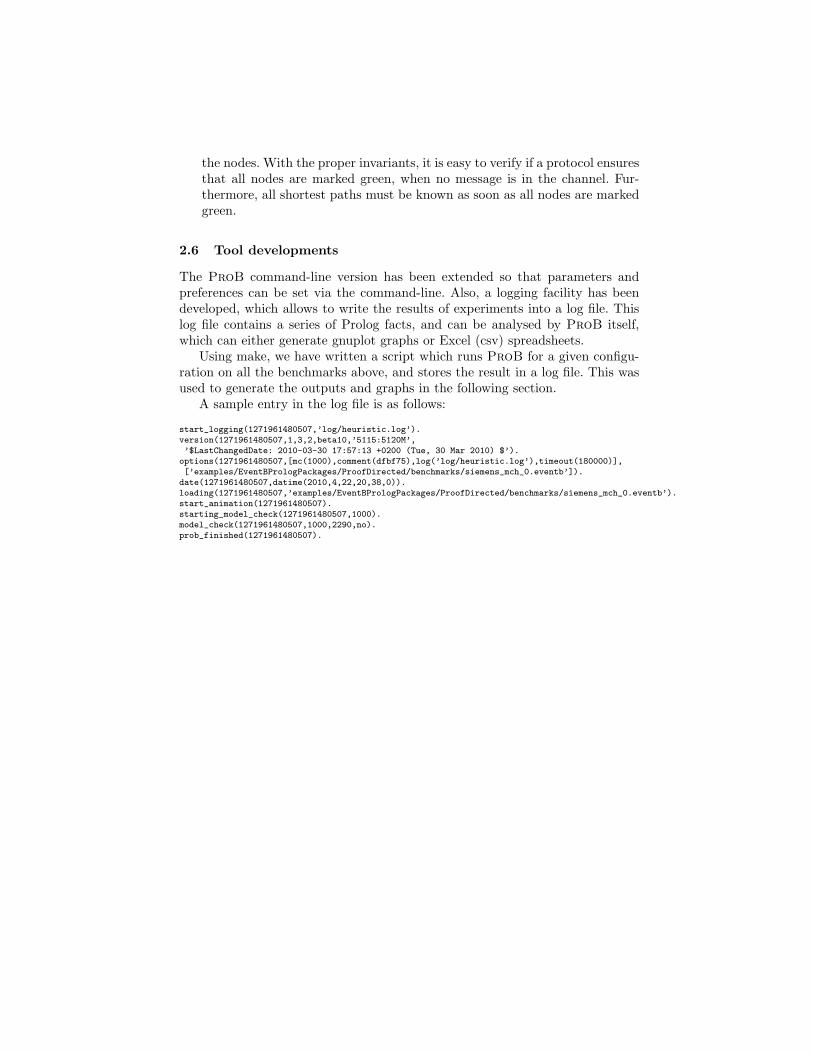
The ProB command-line version has been extended so that parameters andpreferences can be set via the command-line. Also, a logging facility has beendeveloped, which allows to write the results of experiments into a log file. Thislog file contains a series of Prolog facts, and can be analysed by ProB itself,which can either generate gnuplot graphs or Excel (csv) spreadsheets.
Using make, we have written a script which runs ProB for a given configu-ration on all the benchmarks above, and stores the result in a log file. This wasused to generate the outputs and graphs in the following section.
A sample entry in the log file is as follows:
start_logging(1271961480507,’log/heuristic.log’).version(1271961480507,1,3,2,beta10,’5115:5120M’,’$LastChangedDate: 2010-03-30 17:57:13 +0200 (Tue, 30 Mar 2010) $’).
options(1271961480507,[mc(1000),comment(dfbf75),log(’log/heuristic.log’),timeout(180000)],[’examples/EventBPrologPackages/ProofDirected/benchmarks/siemens_mch_0.eventb’]).
date(1271961480507,datime(2010,4,22,20,38,0)).loading(1271961480507,’examples/EventBPrologPackages/ProofDirected/benchmarks/siemens_mch_0.eventb’).start_animation(1271961480507).starting_model_check(1271961480507,1000).model_check(1271961480507,1000,2290,no).prob_finished(1271961480507).

3 Workpackage E1: Empirical Evaluation
3.1 Initial Motivation: Model Checking High-level versus Low-levelSpecifications
Most model checking tools work on relatively low-level formalisms. E.g., themodel checker smv [43, 13] works on a description language well suited for spec-ifying hardware systems. The model checker SPIN [28, 30, 9] accepts the Promelaspecification language, whose syntax and datatypes have been influence by theprogramming language C. Recently, however, there have also been model check-ers which work on higher-level formalisms, such as ProB [36, 38] which acceptsB [1]. Other tools working on high-level formalisms are, for example, fdr [25]for CSP and alloy [33] for a formalism of the same name (although they bothare strictly speaking not model checkers).
It is relatively clear that a higher level specification formalism enables a moreconvenient modelling. On the other hand, conventional wisdom would dictatethat a lower-level formalism will lead to more efficient model checking. However,our own experience has been different. During previous teaching and researchactivities, we have accumulated anecdotal evidence that using a high-level for-malism such as B can be much more productive than using a low-level formalismsuch as Promela. Furthermore, quite surprisingly, it turned out that the use of ahigh-level model checker such as ProB was much more effective in practice thanusing a very efficient model checker such as SPIN on the corresponding low-levelmodel.
3.2 A small empirical study
We first tried to put this anecdotal evidence on a more firm empirical footing, bysystematically comparing the development and validation time of B models withthat of the corresponding Promela models. [57, 49] studies the elaboration of B-models for ProB and Promela models for SPIN on ten different problems. Withone exception (the Needham-Schroeder public key protocol), all B-models aremarkedly more compact than the corresponding Promela models. On average,the Promela models were 1.85 longer (counting the number of symbols). Thetime required to develop the Promela models was about 2-3 times higher thanfor the B models, and up to 18 times higher in extreme cases. No model tookless time in Promela. Some models could not be fully completed in Promela.The study also found that in practice both model checkers ProB and SPIN werecomparable in model checking performance, despite ProB working on a muchhigher-level input language and being much slower when looking purely at thenumber of states that can be stored and processed.
Other independent experimental evaluations also report good performanceof ProB compared against SMV.

3.3 Looking for Answers
Within this project we first tried to analyse and understand the counter-intuitivebehaviour described above in subsection 3.2. The results have been published in[35].
Granularity One tricky issue is the much finer granularity of low-level models.If one is not careful, the number of reachable states can explode expponentially,compared to a corresponding high-level model.
In summary, translating high-level models into Promela is often far fromtrivial. Additional intermediate states and additional state variables are some-times unavoidable. When writing Promela models, for example, great care hasto be taken to make use of atomic (or even dstep) primitives and resetting deadtemporary variables to default values. However, restrictions of atomic make itsometimes very difficult or impossible to hide all of the intermediate states. Moredetails can be found in [35].
Searching for Errors in Large State Spaces Let us disregard the granularityissue and let us look at simple problems, with simple datatypes, which can beeasily translated from B to Promela, so that we have a one-to-one correspondenceof the states of the models. In such a setting, it is obvious to assume that theSPIN model checker for Promela will outperform the B model checker by severalorders of magnitude. Indeed, SPIN generates a specialised model checker in Cwhich is then compiled, whereas ProB uses an interpreter written in Prolog.Furthermore, SPIN has accrued many optimisations over the years, such as partialorder reduction [31, 46] and bitstate hashing [29].
However, it is our experience that even in this setting, this potential speedadvantage of SPIN often does not necessarily translate into better performancein practice in real-life scenarios. Indeed—contrary to what may be expected—we show in this section that SPIN sometimes fares quite badly when used as adebugging tool, rather than as verification tool. Especially for software systems,verification of infinite state systems cannot be done by model checking (withoutabstraction). Here, model checking is most useful as a debugging tool: trying tofind errors in a very large state space.
One experiment reported on in [35] is the NastyVendingMachine (see Sec-tion 2). It has a very large state space, where there is a systematic error inone of the operations of the model (as well as a deadlock when all tickets havebeen withdrawn). To detect the error, it is important to enable this operationand then exercise this operation repeatedly. It is not important to generate longtraces of the system, but it is important to systematically execute combinationsof the individual operations. This explains why depth-first behaves so badly onthis model, as it will always try to exercise the first operation of the model first(i.e., inserting the 10 cents coin). Note that a very large state space is a typicalsituation in software verification (sometimes the state space is even infinite).
In a corrected non-deadlocking model of the vending machine, the state spaceis again very large, but here the error occurs if the system runs long enough;

it is not very critical in which order operations are performed, as long as thesystem is running long enough. This explains why for this model breadth-firstwas performing badly, as it was not generating traces of the system which werelong enough to detect the error.
In order to detect both types of errors with a single model checking algorithm,ProB has been using a mixed depth-first and breadth-first search [38]. Moreprecisely, at every step of the model checking, ProB randomly chooses betweena depth-first and a breadth-first step. This behaviour is illustrated in Fig. 1,where two different possible runs of ProB are shown after exploring 5 nodes ofthe B model from [35].
initialise_machine(0,0,0,0,0,0,2)
insert_10cents insert_20cents insert_50centsinsert_100centsinsert_200centsinsert_card
insert_10cents insert_20cents
insert_50cents
insert_100centsinsert_200cents insert_10centsinsert_20cents insert_50centsinsert_100cents insert_200centsinsert_10cents
insert_20centsinsert_50centsinsert_100centsinsert_200cents
insert_10centsinsert_20centsinsert_50centsinsert_100centsinsert_200cents
initialise_machine(0,0,0,0,0,0,2)
insert_10cents insert_20centsinsert_50centsinsert_100centsinsert_200centsinsert_card
insert_10cents insert_20centsinsert_50centsinsert_100centsinsert_200cents insert_10centsinsert_20centsinsert_50centsinsert_100centsinsert_200cents
insert_10cents insert_20centsinsert_50centsinsert_100centsinsert_200cents insert_10centsinsert_20centsinsert_50centsinsert_100centsinsert_200cents
Fig. 1. Two different explorations of ProB after visiting 5 nodes of the NastyVend-ingmachine
The motivation behind ProB’s heuristic is that many errors in softwaremodels fall into one of the following two categories:
– Some errors are due to an error in a particular operation of the system; henceit makes sense to perform some breadth-first exploration to exercise all theavailable functionality. In the early development stages of a model, this kindof error is very common.
– Some errors happen when the system runs for a long time; here it is oftennot so important which path is chosen, as long as the system is runninglong enough. An example of such an error is when a system fails to recoverresources which are no longer used, hence leading to a deadlock in the longrun.
In summary, if the state space is very large, SPIN’s depth-first search canperform very badly as it fails to systematically test combinations of the variousoperations of the system. Even partial order reduction and bitstate hashing donot help. Similarly, breadth-first can perform badly, failing to locate errors thatrequire the system to run for very long. We have argued that ProB’s combineddepth-first breadth-first search with a random component does not have thesepitfalls.

3.4 Depth-First versus Breadth-First: A thorough empiricalEvaluation
We report on a first extensive empirical evaluation of directed model checkingapproaches for B and Event-B. The experiments for parallel model checking usingthe first prototype are still being undertaken, and will be reported on later.
First task was to compare depth-first versus breadth-first, as well as thedefault mixed depth-first/breadth-first approach of ProB.
The results are summarised in Tables 1–4. Relative times are computed withProB in default settings (which up to know was a mixed depth-first/breadth-first strategy with one-third probability of doing depth-first; more on that below).The experiments were run on a MacBook Pro with a 3.06 GHz Core2 Duoprocessor, and ProB 1.3.2 compiled with SICStus Prolog 4.1.2.
Pure Depth-First In a considerable number of cases pure depth-first is thefastest method, e.g., for the Peterson err, Abrial Earely3 v5, Alstom axl3, andBlocksWorld benchmarks.
However, we can see in Figure 1 that for some models Depth-First fares verybadly:
– In Alstom ex7 in Figure 2, pure depth-first search even fails to find thedeadlock when given an hour of cputime. This real-life example thus supportsour claim from [35] and subsection 3.3 that when state space is too large toexamine fully, depth-first will sometimes not find a counter example. Thisis actually a quite common case for industrial models: they are typically (atleast before abstraction) too large to handle fully.
– Another similar example is Abrial Press m13 in Figure 3, where pure depth-first is about 900 times slower than ProB in the reference settings.
– Another bad example is Puzzle8, where depth-first is more than 7 timesslower or Simpson4Slot where it is 163 times slower than ProB in the ref-erence settings. Finally, for the artificially constructed BFTest, depth-firstsearch fails to find the invariant violation.
For finding goals, the geometric mean was 0.92, i.e., slightly better than thereference setting. Overall, pure depth-first seemed to fare best for the deadlockingmodels with a geometric mean of 0.43. For finding invariant violations, however,the geometric mean was 1.03, i.e., slightly worse than the reference setting.
The bad performance in the Huffman benchmark is actually not relevant:here not all nodes were evaluated. As such, the time to examine 10,000 nodeswas measured. The pure-depth first search here encountered more complicatedstates, than the other approaches, explaining the additional time required formodel checking.
In conclusion, the performance of pure depth-first alone can vary quite dra-matically, from very good to very bad. A such, pure depth first search is not agood choice as a default setting of ProB. Note, however, that we allow the userto override the default setting and put ProB into pure depth-first mode.

Pure Breadth-First In most cases pure Breadth-First is worse than the ref-erence setting; in some cases considerably so. The geometric mean was alwaysabove 1, i.e., worse than the reference setting.
For Alstom ex7 pure breadth-first also fails to find the deadlock.Peterson err in Figure 1 gives a similar picture, Breadth-First being 134
times slower than DF and 11 times slower than the reference settings of ProB.Other examples where BF is not so good: Abrial Earley3 v5, DiningPhil, Syste-mOnChip Router, Wegenetz.
There are some more examples where it performs considerably better thanpure depth-first: Puzzle8, Simpson4Slot, Abrial Press m13 and the “artificial”benchmarks BFTest and DFTest2.
In conclusion, breadth-first on its own is not appropriate, except in specialcircumstances. Note, a user can set ProB into breadth-first mode, but the de-fault is another setting (see below).
Mixed Mixed Depth-first/Breadth-first The motivation behind ProB’smixed depth-first/breadth-first heuristic is that many errors in software modelsfall into one of the following two categories:
– Some errors are due to an error in a particular operation of the system; henceit makes sense to perform some breadth-first exploration to exercise all theavailable functionality. In the early development stages of a model, this kindof error is very common.
– Some errors happen when the system runs for a long time; here it is oftennot so important which path is chosen, as long as the system is runninglong enough. An example of such an error is when a system fails to recoverresources which are no longer used, hence leading to a deadlock in the longrun.
An interesting real-life benchmark is Alstom ex7: here both pure depth-firstand pure breadth-first fail to find the deadlock. However, the mixed strategyfinds the deadlock.
We have experimented with four different versions of the mixed strategy:DF75, DF50, DF33, DF25. The reference setting was DF33, where there is a33 % chance of going depth-first at each step. Best overall geometric mean isobtained when using DF50 (which is now the new default setting of ProB).
In summary, let us look at the radar plots in Figure 2, where we summarisethe results for pure depth-first, pure breadth-first, the old reference setting andthe new one. We can clearly see the quite erratic performance of pure depth-first (relative to the reference setting), and the less erratic but usually worseperformance of pure breadth-first. We can also see that the new reference settingusually lies within the reference setting circle, smoothing out most of the (bad)erratic behaviour of the pure depth-first approach.
The Houseset benchmark clearly shows that mixed DF/BF has problem goingdeep if there is a large branching factor. This may indicate a possible way toimprove our current algorithm, by favouring at least some very deep paths.

0.0
0.1
1.0
10.0 SchedulerErr
Simpson4Slot
Peterson_err
TravelAgency
SecureBldg_M21_err3
Abrial_Press_m2_err
SAP_M_Partner
Needham-‐Schroeder
NastyVending
Houseset
BFTest
DFTest1
DFTest2
GEOMEAN
DF Rel.
DF50 Rel.
DF33 Rel.
BF Rel.
0.0
0.1
1.0
10.0 Abrial_Earley3_v3
Abrial_Earley3_v5
Abrial_Earley4_v3
Alstom_axl3
Alstom_ex7
Bosch_CrsCtl
SAP_MChoreography
DiningPhil
CXCC0
GEOMEAN
DF Rel.
DF50 Rel.
DF33 Rel.
BF Rel.
0.0
0.1
1.0
10.0 RussianPostal
TrainTorch
BlocksWorld
Farmer
Hanoi
Puzzle8
RushHour
Abrial_Press_m13
Abrial_Queue_m1
SystemOnChip_Router
Wegenetz
GEOMEAN
DF Rel.
DF50 Rel.
DF33 Rel.
BF Rel.
Fig. 2. Radar plot for invariant, deadlock and goal checking (DF/BF Analysis)
3.5 Evaluation the potential of using Heuristics
Directed Model Checking uses additional information about the model or thedestination state in form of a heuristic that guides the model checker towardsa target state. This additional information can be collected using for instancestatic analysis or it can be given by the modeler.
Currently the state space of ProB is stored as a Prolog fact database. Everystate can be quickly accessed using its ID or using the hash-value of its state;see Figure 3 The model checker also maintains a pending list of open nodes,using two predicates: retracting a fact from one of the predicates yields the leastrecently added open node (for depth-first traversal) and rectracting from theother predicate yields the oldest open node (for breadth-frist traversal). Thisapproach allowed us to implement a mixed depth-first / breadth-first approachby randomly selecting either an element from the front or the end of the pendinglist of open nodes.
We have implemented a priority queue in C++ using the STL (StandardTemplate Library) multimap data structure. One can thus efficiently add newopen nodes with a particular weight, and then either chose the node with thelowest or highest weight.
We evaluated some strategies to assign weights to newly encountered nodes.In particular a random search, a search based on the number of successor states,a search based on the (term)size of the state as well as some custom heuristic
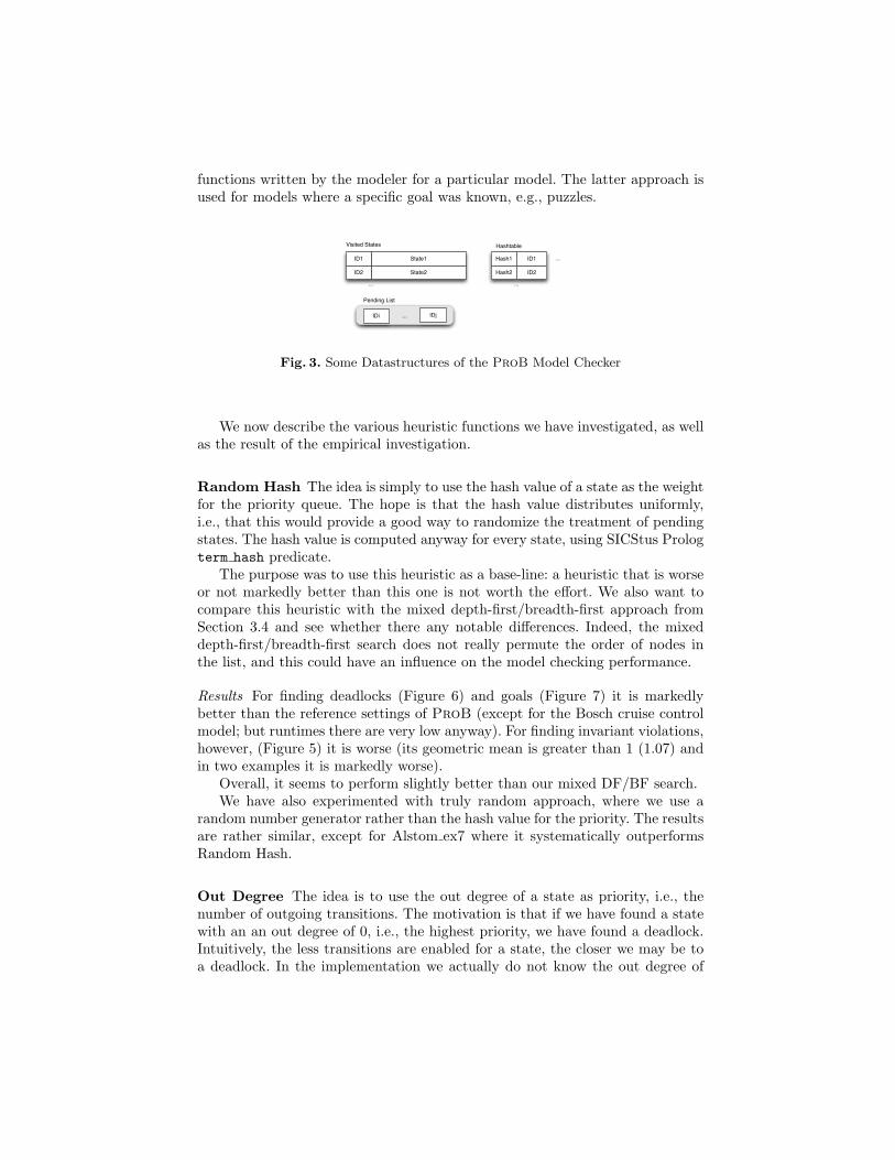
functions written by the modeler for a particular model. The latter approach isused for models where a specific goal was known, e.g., puzzles.
ID1 State1 ID1Hash1
Visited States Hashtable
...
Pending List
IDi ... IDj
ID2 State2 ID2Hash2
... ...
Fig. 3. Some Datastructures of the ProB Model Checker
We now describe the various heuristic functions we have investigated, as wellas the result of the empirical investigation.
Random Hash The idea is simply to use the hash value of a state as the weightfor the priority queue. The hope is that the hash value distributes uniformly,i.e., that this would provide a good way to randomize the treatment of pendingstates. The hash value is computed anyway for every state, using SICStus Prologterm hash predicate.
The purpose was to use this heuristic as a base-line: a heuristic that is worseor not markedly better than this one is not worth the effort. We also want tocompare this heuristic with the mixed depth-first/breadth-first approach fromSection 3.4 and see whether there any notable differences. Indeed, the mixeddepth-first/breadth-first search does not really permute the order of nodes inthe list, and this could have an influence on the model checking performance.
Results For finding deadlocks (Figure 6) and goals (Figure 7) it is markedlybetter than the reference settings of ProB (except for the Bosch cruise controlmodel; but runtimes there are very low anyway). For finding invariant violations,however, (Figure 5) it is worse (its geometric mean is greater than 1 (1.07) andin two examples it is markedly worse).
Overall, it seems to perform slightly better than our mixed DF/BF search.We have also experimented with truly random approach, where we use a
random number generator rather than the hash value for the priority. The resultsare rather similar, except for Alstom ex7 where it systematically outperformsRandom Hash.
Out Degree The idea is to use the out degree of a state as priority, i.e., thenumber of outgoing transitions. The motivation is that if we have found a statewith an an out degree of 0, i.e., the highest priority, we have found a deadlock.Intuitively, the less transitions are enabled for a state, the closer we may be toa deadlock. In the implementation we actually do not know the out degree of
a node until it has been processed. Hence, we use the out degree of the (first)predecessor node for the priority.
Results Indeed, for finding deadlocks this heuristic obtained the best geometricmean of 0.5. So, this simple heuristic works surprisingly well. For finding goals,this heuristic still obtains geometric mean of 0.63, but it is worse than therandom hash function. For finding invariant violations it does not work at all;its geometric mean is 1.56.
A further refinement of this heuristic is to combine the out degree with therandom hash heuristic, i.e., if two nodes have the same out degree (which canhappen quite often) we use the hash value as heuristic to avoid a degenerationinto depth-first search. This refinement leads to a further performance improve-ment for deadlock finding (geometric mean of 0.34 compared to 0.50), and forgoal finding. But it is markedly worse for invariant violation finding.
In conclusion, the out degree heuristic, especially when combined with ran-dom hash, works surprisingly well for its intended purpose of finding deadlocks.In future work, we plan to further refine this approach, by using a static flowanalysis to guide model checker into deadlocks and/or particular enablings forevents.
Term Size The idea of this heuristic is to use the term size of the state (i.e.,the number of constant and function symbols appearing in its representation)as priority. The motivation for this heuristic is that the larger the state is, themore complicated it will be to process (for checking invariants and computingoutgoing transitions). Hence, the idea is to process simpler states first, in anattempt to maximise the number of nodes processed per time unit.
Results For finding goals this heuristic has a geometric mean of 0.85, i.e., it isbetter than the reference setting of ProB, but worse than random hash. Fordeadlock and invariant checking, it also performs worse than random hash. Insummary, this heuristic does not seem worth pursuing further.
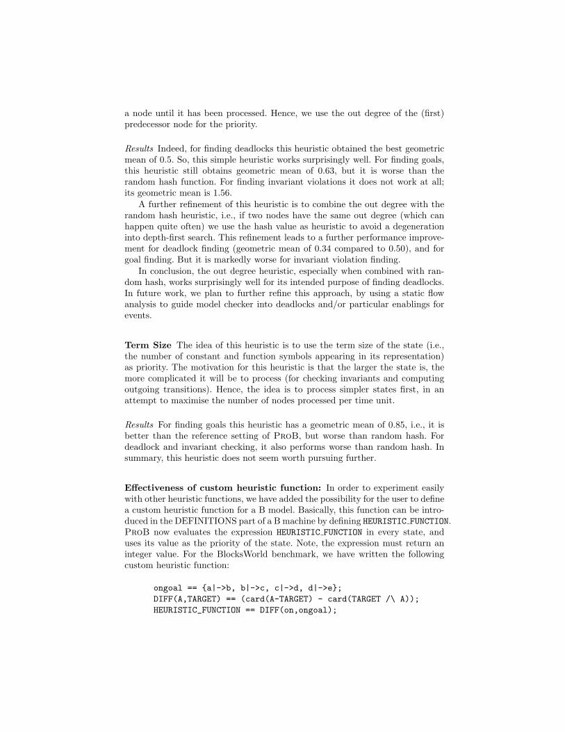
Effectiveness of custom heuristic function: In order to experiment easilywith other heuristic functions, we have added the possibility for the user to definea custom heuristic function for a B model. Basically, this function can be intro-duced in the DEFINITIONS part of a B machine by defining HEURISTIC FUNCTION.ProB now evaluates the expression HEURISTIC FUNCTION in every state, anduses its value as the priority of the state. Note, the expression must return aninteger value. For the BlocksWorld benchmark, we have written the followingcustom heuristic function:
ongoal == {a|->b, b|->c, c|->d, d|->e};DIFF(A,TARGET) == (card(A-TARGET) - card(TARGET /\ A));HEURISTIC_FUNCTION == DIFF(on,ongoal);

Note the machine as a variable on is of type Objects +-> Objects and theGOAL for the model checker is to find a state where on = ongoal is true.
In the benchmarks, we have mainly written heuristic functions which esti-mate the distance between a target goal state and the current state. In future,we plan to derive the definition of those heuristic functions automatically. Asimple distance heuristic, can be derived if the goal of the model checking is tofind specific values for certain variables of the machine (such as on = ongoal).Basically, for current state s = 〈s1, . . . , sn〉 and a target state t = 〈t1, . . . , tn〉 weuse as heuristic h(s) = Σ1≤i≤n∆(si, ti) where
– ∆(x, target) = abs(x− target) if x integer– ∆(x, target) = card(x− TARGET )− card(TARGET ∩A) if x a set– ∆((x, y), (t1, t2)) = ∆(x, t1) +∆(y, t2) for pairs,– in all other cases: ∆(x, target) = 0 if x = target and 1 otherwise
If the value of a particular variable is not relevant, then we simply set ∆(si, ti) =0 for that variable.
This defines a kind of Hamming distance for B states. We have applied this(manually) in the BlocksWorld example above.
We have only evaluated this approach for finding goals. Here, it obtainedthe best overall geometric mean of 0.34. For Puzzle8 and Abrial press m13,this approach yielded by far the best solution. For RussianPostal, TrainTorch,Blocksworld, Abrial Queue m1 it obtains the best result. There was one exper-iment were it is markedly worse than ProB in the reference settings: Syste-mOnChip Router. Here the heuristic did not pay off at all. Indeed, here the lastevent changes all of the four variables, relevant for the model checking GOAL,in one step. This only confirms the fact that we are working with heuristic func-tions, which are not guaranteed to always improve the performance.
Summary of heuristic function experiments: We have summarised themain findings of our experiments in Figure 4. We can conclude that:
– for invariant checking, the random hash heuristic fared best.7 This seems toindicate that it is maybe useful to combine some more random componentinto the depth-first/breadth-first techniques of Section 3.4, e.g., to also ran-domly permute the operation order. Indeed, the approaches from Section 3.4always process the operations in the same order, and does not shuffle thestates inside the pending list.
– for deadlock checking, the out-degree-hash heuristic is the best. It shouldprovide a good basis for further improved deadlock checking techniques.
– for goal finding, a custom heuristic function provides (except in one case)by far the best result. The next step is to derive those heuristic functionsautomatically.
7 However, note that DF50 had an overall geometric mean of 0.58, and was hencebetter overall than random hash.

0.01
0.10
1.00
10.00 SchedulerErr
Simpson4Slot
Peterson_err
TravelAgency
SecureBldg_M21_err3
Abrial_Press_m2_err
SAP_M_Partner Needham-‐Schroeder
Houseset
BFTest
DFTest1
DFTest2
GEOMEAN
DF33_BF66
HashRand
OutDegree
OutDegHash
0.01
0.10
1.00
Abrial_Earley3_v3
Abrial_Earley3_v5
Abrial_Earley4_v3
Alstom_axl3
Alstom_ex7
Bosch_CrsCtl
SAP_MChoreography
DiningPhil
CXCC0
GEOMEAN
DF33_BF66
HashRand
OutDegree
OutDegHash
0.01
0.10
1.00
10.00 RussianPostal
TrainTorch
BlocksWorld
Farmer
Hanoi
Puzzle8
RushHour
Abrial_Press_m13
Abrial_Queue_m1
SystemOnChip_Router
Wegenetz
GEOMEAN
DF33_BF66
OutDegHash
CUSTOM
Fig. 4. Radar plot for invariant, deadlock and goal checking (Heuristic Analysis)
The out-degree-hash heuristic also provides reasonably good performance(its geometric mean is 0.41, which is better than the best mixed-depth-firstone of 0.57 for DF75).
3.6 Overall Conclusions of all Experiments
– The mixed depth-breadth-first strategy is a good idea, it is much more robustthan either depth-first and breadth-first. Still, it may be useful to improvethe approach by randomising the order of transitions and by favouring somevery deep paths.
– The use of heuristics can pay off considerably. The out-degree heuristic wassuccessful for deadlock checking, while measuring a distance to a target statewas generally very successful for goal finding tasks.Still, more refined heuristics are required to fully exploit the potential. Itis probably a good idea to use control flow graph information to guide themodel checker more precisely.
3.7 Experimental Results (Figures and Tables)
Note: we use geometric mean [24], as the arithmetic mean is useless for nor-malised results. Of course, the geometric mean itself should also be taken with agrain of salt (various articles also attack its usefulness). Indeed, without know-ing how representative the chosen benchmarks are for the overall population of

B specifications, we can conclude little. In Section 2 we have tried to assem-ble a variety of benchmarks from our own experience; but this sample may beinadequate for other application scenarios.
Thus, we also provide all figures in the tables below, so that minimum, max-imum relative runtimes can be seen, as well as the absolute runtime of thereference benchmark. Indeed, the relative runtimes are less reliable, when theabsolute runtime of the reference benchmark is already very low.

Invariant Benchmark DF DF75 DF50 DF33 (abs+rel) DF25 Rel BF
SchedulerErr 0.33 0.33 0.33 30 ms 1.00 1.00 2.67Simpson4Slot 163.33 0.22 0.67 90 ms 1.00 0.78 2.11Peterson err 0.08 0.08 0.22 360 ms 1.00 3.06 11.17TravelAgency 0.16 0.27 0.10 630 ms 1.00 0.78 2.43SecureBldg M21 err3 0.50 0.50 1.00 20 ms 1.00 1.00 1.00Abrial Press m2 err 0.26 3.38 0.34 880 ms 1.00 1.81 1.26SAP M Partner 0.58 1.08 1.00 120 ms 1.00 0.92 0.83NastyVending 0.02 0.08 8.00 130 ms 1.00 2.85 1.00NeedhamSchroeder 1.28 1.52 0.95 22620 ms 1.00 0.70 1.37Houseset 0.05 0.06 0.22 2610 ms 1.00 2.66 ** 336.27BFTest ** 15000.00 11592.75 0.75 80 ms 1.00 1.00 0.88DFTest1 0.20 0.35 0.71 2360 ms 1.00 1.01 1.02DFTest2 7.86 0.50 0.60 2930 ms 1.00 0.99 1.00
GEOMEAN 1.03 0.78 0.58 394 ms 1.00 1.24 2.35DF: out of memory
0.0
0.1
1.0
10.0
100.0
1000.0
10000.0
SchedulerErr
Simpson4Slot
Peterson_err
TravelAgency
SecureBldg_M21_err3
Abrial_Press_m2_err
SAP_M_Partner
Needham-‐Schroeder
NastyVending
Houseset
BFTest
DFTest1
DFTest2
GEOM
EAN
DF Rel.
DF75 Rel.
DF50 Rel.
DF33 Rel.
DF25 Rel
BF Rel.
Table 1. Relative times for checking models with invariant violations (DF/BF Anal-ysis)

Deadlock Benchmark DF DF75 DF50 DF33 (abs+rel) DF25 Rel BF
Abrial Earley3 v3 0.33 0.44 0.93 270 ms 1.00 1.19 1.19Abrial Earley3 v5 0.13 0.32 0.75 4320 ms 1.00 2.18 7.95Abrial Earley4 v3 0.89 0.89 1.00 90 ms 1.00 1.00 1.00Alstom axl3 0.10 0.17 0.20 51270 ms 1.00 3.51 14.61Alstom ex7 ** 4.20 0.23 0.35 856320 ms 1.00 ** 1.21 ** 3.00Bosch CrsCtl 1.00 1.00 1.00 3 ms 1.00 4.00 4.00SAP MChoreography 0.50 0.50 0.50 20 ms 1.00 1.00 1.00DiningPhil 0.13 0.26 0.36 1690 ms 1.00 2.49 6.20CXCC0 0.50 1.00 1.00 10 ms 1.00 2.00 2.00
GEOMEAN 0.43 0.44 0.59 540 ms 1.00 1.82 3.02AVG 0.00 0.00 0.00 0 ms 0.00 0.00 0.00
0.0
0.1
1.0
10.0
Abrial_Earley3_v3
Abrial_Earley3_v5
Abrial_Earley4_v3
Alstom_axl3
Alstom_ex7
Bosch_CrsCtl
SAP_MChoreography
DiningPhil
CXCC0
GEOM
EAN
DF Rel.
DF75 Rel.
DF50 Rel.
DF33 Rel.
DF25 Rel
BF Rel.
Table 2. Relative times for checking models with deadlocks (DF/BF Analysis)

Goal Benchmark DF DF75 DF50 DF33 (abs+rel) DF25 Rel BF
RussianPostal 0.95 0.14 0.73 220 ms 1.00 1.05 1.50TrainTorch 1.14 1.17 0.69 350 ms 1.00 1.06 0.94BlocksWorld 0.07 0.25 1.16 440 ms 1.00 1.18 1.07Farmer 0.50 1.00 0.50 20 ms 1.00 1.00 1.00Hanoi 0.54 0.48 1.00 500 ms 1.00 0.84 0.90Puzzle8 7.56 2.86 0.40 59060 ms 1.00 0.11 0.71RushHour 0.41 0.66 0.90 127020 ms 1.00 1.09 1.11Abrial Press m13 899.78 1.64 1.26 800 ms 1.00 0.66 2.23Abrial Queue m1 1.60 3.00 1.00 50 ms 1.00 1.60 1.40SystemOnChip Router 0.05 0.14 0.08 2050 ms 1.00 1.04 1.45Wegenetz 0.08 0.08 0.25 120 ms 1.00 0.17 2.58
GEOMEAN 0.92 0.57 0.58 715 ms 1.00 0.71 1.26
0.0
0.1
1.0
10.0
100.0
RussianPostal
TrainTorch
BlocksWorld
Farmer
Hanoi
Puzzle8
RushHour
Abrial_Press_m13
Abrial_Queue_m1
SystemO
nChip_Router
Wegenetz
GEOM
EAN
DF Rel.
DF75 Rel.
DF50 Rel.
DF33 Rel.
DF25 Rel
BF Rel.
Table 3. Relative times for checking models with goals to be found (DF/BF Analysis)

No Error Benchmark DF DF75 DF50 DF33 (abs+rel) DF25 Rel BF
Scheduler1 1.00 1.00 1.00 6010 ms 1.00 1.00 1.00Volvo Cruise 1.01 1.01 1.01 5360 ms 1.00 1.00 1.00USB4 1.00 1.00 1.00 3270 ms 1.00 1.00 1.00Nokia Nota 1.09 1.03 1.01 44220 ms 1.00 1.00 1.00Huffman 17.98 1.15 1.05 11100 ms 1.00 1.00 0.98Cansell Contention 1.00 1.01 1.01 1490 ms 1.00 1.01 1.01Demoney GS R1 1.00 1.01 1.00 1580 ms 1.00 1.00 1.00SystemOnChip Router 0.99 1.00 1.00 27020 ms 1.00 1.00 1.01Mondex m2 1.10 0.95 0.96 1700 ms 1.00 1.02 1.14Mondex m3 1.09 0.95 0.96 1910 ms 1.00 1.01 1.12Siemens ATP0 1.12 1.10 1.00 2090 ms 1.00 0.98 0.93SSF obsw1 1.10 1.05 1.04 22500 ms 1.00 1.00 1.00Echo 0.98 0.98 1.00 440 ms 1.00 1.00 1.00ETH Elevator12 0.83 0.86 0.93 106520 ms 1.00 1.01 0.90
GEOMEAN 1.25 1.00 1.00 6687 ms 1.00 1.00 1.01
0.1
1.0
10.0
100.0
Scheduler1
Volvo_Cruise
USB4
Nokia_Nota
Huffman
Cansell_Conten?on
Demoney_GS_R1
SystemO
nChip_Router
Mondex_m2
Mondex_m3
Siemens_ATP0
SSF_obsw1 Echo
ETH_Elevator12
GEOM
EAN
DF Rel.
DF75 Rel.
DF50 Rel.
DF33 Rel.
DF25 Rel
BF Rel.
Table 4. Relative times for checking models without errors (DF/BF Analysis)
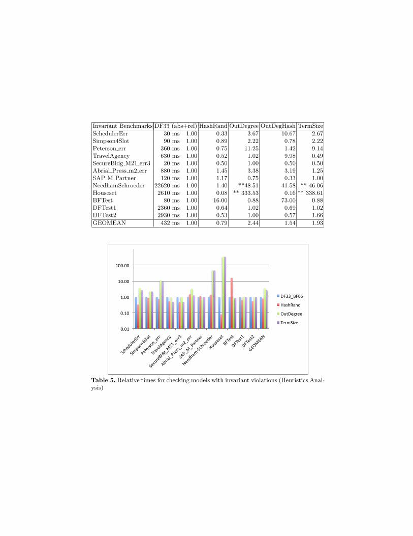
Invariant Benchmarks DF33 (abs+rel) HashRand OutDegree OutDegHash TermSize
SchedulerErr 30 ms 1.00 0.33 3.67 10.67 2.67Simpson4Slot 90 ms 1.00 0.89 2.22 0.78 2.22Peterson err 360 ms 1.00 0.75 11.25 1.42 9.14TravelAgency 630 ms 1.00 0.52 1.02 9.98 0.49SecureBldg M21 err3 20 ms 1.00 0.50 1.00 0.50 0.50Abrial Press m2 err 880 ms 1.00 1.45 3.38 3.19 1.25SAP M Partner 120 ms 1.00 1.17 0.75 0.33 1.00NeedhamSchroeder 22620 ms 1.00 1.40 **48.51 41.58 ** 46.06Houseset 2610 ms 1.00 0.08 ** 333.53 0.16 ** 338.61BFTest 80 ms 1.00 16.00 0.88 73.00 0.88DFTest1 2360 ms 1.00 0.64 1.02 0.69 1.02DFTest2 2930 ms 1.00 0.53 1.00 0.57 1.66
GEOMEAN 432 ms 1.00 0.79 2.44 1.54 1.93
0.01
0.10
1.00
10.00
100.00
SchedulerErr
Simpson4Slot
Peterson_err
TravelAgency
SecureBldg_M21_err3
Abrial_Press_m2_err
SAP_M_Partner
Needham-‐Schroeder
Houseset
BFTest
DFTest1
DFTest2
GEOM
EAN
DF33_BF66
HashRand
OutDegree
TermSize
Table 5. Relative times for checking models with invariant violations (Heuristics Anal-ysis)

Deadlock Benchmarks DF33 (abs+rel) HashRand OutDegree OutDegHash TermSize
Abrial Earley3 v3 270 ms 1.00 0.74 1.22 0.70 1.22Abrial Earley3 v5 4320 ms 1.00 0.41 5.88 0.16 7.95Abrial Earley4 v3 90 ms 1.00 0.89 1.00 0.89 1.00Alstom axl3 51270 ms 1.00 0.82 0.09 0.16 0.08Alstom ex7 856320 ms 1.00 0.55 ** 1.91 1.10 **1.57Bosch CrsCtl 3 ms 1.00 8.00 1.00 1.00 4.00SAP MChoreography 20 ms 1.00 0.50 0.50 0.50 1.00DiningPhil 1690 ms 1.00 1.16 0.05 0.03 1.59CXCC0 10 ms 1.00 0.25 0.25 0.25 0.25
GEOMEAN 432 ms 1.00 0.80 0.58 0.34 1.07
0.01
0.10
1.00
10.00
Abrial_Earley3_v3
Abrial_Earley3_v5
Abrial_Earley4_v3
Alstom_axl3
Alstom_ex7
Bosch_CrsCtl
SAP_MChoreography
DiningPhil
CXCC0
GEOM
EAN
DF33_BF66
HashRand
OutDegree
TermSize
OutDegHash
Table 6. Relative times for checking models with deadlocks (Heuristics Analysis)

Goal Benchmarks DF33 (abs+rel) HashRand OutDegree OutDegHash TermSize CUSTOM
RussianPostal 220 ms 1.00 0.45 0.77 0.36 1.18 0.45TrainTorch 350 ms 1.00 0.97 0.26 1.14 0.20 0.20BlocksWorld 440 ms 1.00 1.16 0.07 0.07 1.20 0.02Farmer 20 ms 1.00 1.00 1.00 0.50 1.00 1.00Hanoi 500 ms 1.00 0.52 0.92 0.52 0.90 0.34Puzzle8 59060 ms 1.00 20.54 1.31 2.69 0.71 0.03RushHour 127020 ms 1.00 0.42 0.60 0.56 1.12 0.79Abrial Press m13 800 ms 1.00 0.49 2.36 2.21 2.48 0.20Abrial Queue m1 50 ms 1.00 0.40 16.60 0.60 2.80 0.40SystemOnChip Router 2050 ms 1.00 0.10 0.05 0.04 1.50 72.42Wegenetz 120 ms 1.00 0.17 0.33 0.08 0.08 0.08
GEOMEAN 715 ms 1.00 0.64 0.63 0.41 0.85 0.34
0.01
0.10
1.00
10.00
RussianPostal
TrainTorch
BlocksWorld
Farmer
Hanoi
Puzzle8
RushHour
Abrial_Press_m13
Abrial_Queue_m1
SystemO
nChip_Router
Wegenetz
GEOM
EAN
DF33_BF66
HashRand
OutDegree
TermSize
CUSTOM
Table 7. Relative times for checking models with goals to be found (Heuristics Anal-ysis)

noerror DF33 (abs+rel) HashRand OutDegree OutDegHash TermSize
Scheduler1 6010 ms 1.00 1.00 1.00 1.00 1.02Volvo Cruise 5360 ms 1.00 1.01 1.00 1.01 1.01USB4 3270 ms 1.00 1.00 0.99 1.00 1.00Nokia Nota 44220 ms 1.00 1.10 0.90 0.92 1.12Huffman 11100 ms 1.00 1.64 1.04 2.09 1.03Cansell Contention 1490 ms 1.00 1.00 1.01 1.01 1.02Demoney GS R1 1580 ms 1.00 1.00 0.99 1.01 1.03SystemOnChip Router 27020 ms 1.00 1.00 0.98 1.00 1.02Mondex m2 1700 ms 1.00 1.03 1.44 1.27 0.97Mondex m3 1910 ms 1.00 1.02 1.39 1.24 0.96Siemens ATP0 2090 ms 1.00 1.81 1.03 0.92 0.93SSF obsw1 22500 ms 1.00 1.12 1.01 1.02 1.19ETH Elevator12 106520 ms 1.00 1.09 0.54 0.56 0.66GEOMEAN 6687 ms 1.00 1.12 1.00 1.04 0.99
Table 8. Relative times for checking models without errors (Heuristics Analysis)

4 Workpackage I1: Generic Parallelisation Prototype
We investigated different approaches for building a parallel version of ProB.Because Multicore platforms become more and more popular we decided to notonly investigate a distributed version of ProB, but also a version that workson multicore platforms. However the lack of thread support in SICStus Prologmakes the implementation of a multicore version more difficult. In this reportwe describe some attempts we tried (i.e., using shared memory for inter processcommunication, using a database) and the lessons we learnt from these proto-types.
4.1 Interfacing with SICStus Prolog
Because SICStus Prolog does not yet support multithreading it is necessary toparallelize the model checking using different processes. To share data amongthese processes we considered the following approaches:
– Share data using socket communication to a Java process.– Share data using the SICStus to C interface.– Share data using direct socket communication between the Prolog Processes.
We use the first approach for interaction of the ProB core and our Plug-infor the Rodin tool. It has the advantage that we could reuse a large numberof frameworks for distributed computing. However when developing the RodinPlug-in we noticed that the communication has a performance impact that istolerable when animating a model but it could become a problem when it comesto more frequent interaction between Java and Prolog during model checking.The Jasper Java interface of SICStus Prolog has turned out to be quite hard tosetup and fragile across different platforms. The second approach was intensivelypursued in the first project phase. It is required in particular when using sharedmemory to communicate between processes running on the same platform. Wereport on this approach in section 4.2. The last method was used in the firstprototype that used a tuple space for communication. The prototype turnedout to be not very robust against changes of the environment, i.e., a process isgetting killed or a network connection is lost. Also the blackboard approach doesonly scale until a certain amount of traffic because of the client server structure.Implementing a more sophisticated concept in pure Prolog does not seems tobe a good idea because it requires to write a lot of functionality from scratch.Instead we want to investigate to use Java as the control layer while Prologprocesses share the data directly.
4.2 Share data using the SICStus C-Interface
ProB uses two main facts to represent the state space. To represent a stateit asserts a visited_expression/2 fact containing a unique id of the nodeand the state itself in a Prolog encoding. We represent a transition using a

transition/3 fact containing the ids of the source and the destination stateand a representation of the transition event, i.e., an encoding of the opetartion’sname and its parameters. We also have a few additional predicates as flags,e.g. invariant_violated/1 to mark all stated that violate the invariant. Thereason for this is that SICStus Prolog does not support multi indexing, i.e.,finding all states violating the invariant would be inefficient if this information isincorporated into the visited_expression fact. However our C representationallows multi indexing therefore we can join all information about a particularstate into a single structure. In addition we gain the possibility to efficientlysearch for incoming transitions. Without duplicating the transition facts thisis not possible using SICStus Prolog.
However the representation in C has also some drawbacks. It is difficult tosupport sharing of data structures. Let us consider the following Prolog predi-cate.
share :- fact(A), fact(B), R=tree(A,B), assert(fact(R)).
If we call share Prolog will fetch the data structures A and B from thedatabase, combine them and store them as a new structure. Notice that Prologdoes not have to copy A and B. The new fact tree(A,B) contains pointers to theoriginal structures. Discovering these structural sharing using the foreign inter-face is difficult because the internal representation is hidden from the interface.
Our prototype implementation stores states and transitions in the memorycontrolled by the C extension rather than Prolog together with some countersand index structures to provide a fast lookup of transitions. To save memory asymbol table mapping atoms to integer values was implemented. Is is also storedin the shared memory. However for the prototype the memory architecture isimplemented as a static structure and has to be configured manually beforecompiling ProB.
Big segments of memory are allocated at startup of ProB and will be filledwhen model checking starts. ProB uses two segments for storing structs of tran-sitions and visited expressions, with some meta information and a pointer tothe term associated with these expressions, the terms are stored in two otherchunks, containing the serialized terms as a string. For indexing transitions bysource and destination three segments are allocated, a src- and dst-array point-ing to an index element list in the third segment. Another segment stores somecounter and the last one is used to store the symbol table.
Prolog terms are represented as a tree and can be accessed on the C-levelwith a hand full of functions provided by SICStus Prolog. Using these functionsit is possible to determine how many arguments a functor has and to get the typeand value of any atom. To flatten a term a recursive function in the extension iscalled and saves the term representing atoms as ids from the symbol table andarity of functors in a string. Saving the additional information of arity is usedto deserialize the string to a tree in a single run.

4.3 Using ProB with shared memory
On Linux and OS X systems we can use the shared memory implementationfor inter process communication (IPC) to share information among processes.The implementation provides functions to allocate, attach and detach sharedmemory segments and to create semaphores for synchronization. The idea is touse distributed shared memory to increase the power of ProB by using moreCPUs and to have more RAM available. Indeed our prototype implementationof the Prolog to C interface already uses shared memory. In combination withOSS we can use the same implementation to get a version of ProB that can beused in a cluster.
4.4 Using Berkely DB
SICStus Prolog contains an interface to the Berkely Database(bdb) Becausethis interface is built in we wanted to evaluate if its performance is sufficient toshare the state space among instances of the ProB process. We had the hopethat SICStus can use faster techniques (i.e., direct copying of memory blocks)than a foreign interface can. We developed a simple prototype to compare theperformance of asserting facts in the Prolog database and storing the facts ina database. We also tried to access the database concurrently with multiplethreads. Storing a million facts into the Berkeley database is about 40 timesslower than asserting them in Prolog. This performance loss is not surprisingbecause the database uses disk I/O while Prolog uses memory. But the approachdoes not scale at all. Using two processes (one only reading and one reading andwriting) the performance of the database collapses writing 100000 facts takesabout 7 seconds using a single process. If we add a process that only reads factsfrom the database writing the same facts takes more than 2 minutes. Becausewe cannot control the way the database is used by Prolog we cannot fine-tuneit, i.e., we cannot exploit the fact that we never remove entries from the statespace. We will not consider using the SICStus bdb library in the future, but itmight be an option to use a distributed database together with the Prolog to Cinterface instead of OSS.
4.5 Combining ProB and Spin
We did investigate using Spin, using Spin’s C-interface to link the ProB inter-preter via Prolog’s C-interface. However, after discussions with Gerhard Holz-mann and Dragan Bosnacki, this avenue seems very tricky as our Prolog inter-preter is inherently non-deterministic.
4.6 Future Work
We currently evaluate if it is reasonable to use the shared memory approach fora multicore version of ProB. We require that the additional costs of storing the
state space in the shared memory can be compensated by sharing the computa-tion among a reasonable low number (i.e., two) processes. Luckily, first resultshave shown that this is the case for the majority of the benchmarks, but thereare also several models where we clearly fail. In some cases the version that usesshared memory is up to 16 times slower than the Prolog version. We suspect thatour rather naive encoding of the state (and in particular the symbol table) is thereason for these problems. However, we are confident that these issues can besolved. The next steps are therefore the optimization of the symbol table and abetter memory management. It is clearly necessary to not allocate huge blocks ofmemory. Instead we want to implement our own page table and manage smallerchunks to get a more scalable system. Furthermore, we plan to port ProB toa distributed memory system using OSS. In addition we started to work on aprototype that uses Java to control communicating Prolog processes. We willnot further pursue the database approach unless the OSS version turns out tobe not sufficient and we will also not consider to combine ProB and Spin.

5 Workpackages T2/I2: Abstract Interpretation of B
During the evolution of the project, we realised that in addition to a “classical”abstract interpretation, we would need a flow analysis. The latter can actuallyalso be viewed as a predicate-abstraction-based abstract interpretation. This isdescribed in Workpackage T3.
As far as classical abstract interpretation is concerned, we have developedand implemented a particular predicate analysis technique to infer intervals forintegers and cardinalities. We describe this in Section 5.1. We have also developeda generic abstract interpretation framework, which approximates the effects ofB operations. We describe this in Section 5.2.
5.1 Predicate Analysis
A static analysis of predicates provides information that can be used in severalcontexts.
– Sometimes the constraint solver has to enumerate all possible values of vari-ables to find values that satisfy a predicate. The additional information canbe used to restrict the search to a subset of such values.
– Some variables can be represented more effectively when additional infoabout the possible values is known. E.g., a relation could be stored as amap if we known that it is a function.
We also plan to use our analysis to enable translation of B predicates to SATsolvers via Kodkod. Finally, we also plan to use our analysis to detect erroneoussettings of MAXINT, MININT in ProB.
The analysis we implemented as a prototype is easily extensible for differentkinds of information and works as follows. For each node in the abstract syntaxtree of a predicate we store an arbitrary number of “inferred information points”,depending of the node’s type. E.g. for an integer expression we store the integerinterval of possible values, identified by intval. For a set, we store the integerinterval of possible cardinalities, identified by card.
Each type of information point can also be used for all elements of a set(elem). E.g. for a set of integers, we can store the cardinality of the set (card)and the integer interval in wich all elements are located (elem:intval).
We generate constraints between those information points by applying pat-tern matching to the syntax tree. E.g. for a predicate x ∈ S we can propagatethe information of each point elem:I(S) to an information point I(x). For apredicate x < y we can propagate the minimum of intval(x) to intval(y) andthe maximum of intval(y) to intval(x).
The prototype’s constraint solving technique is a naıve approach where infor-mation is propagated until a fixpoint or a maximum number of inference stepsis reached. The appliction of modern constraint solving techniques should befuture work.

Example. For the predicate x ∈ 1 .. 10 we generate the following “inferred in-formation points” with their initial values: intval(x) = (−∞,∞), intval(1) =[1, 1], intval(10) = [10, 10], card(1 .. 10) = [0,∞), elem:intval(1 .. 10) =(−∞,∞). For x..y we can propagate the minimum resp. maximum of intval(x)and intval(y) to the node elem:intval(1 .. 10). Additionally we can use theinformation elem:intval(1 ..10) to limit the maximum cardinality card(1 ..10).With the inference rule of membership as presented above, we can derive theinformation: intval(x) = (1, 10), card(1 .. 10) = [0, 10], elem:intval(1 .. 10) =[1, 10]. Whereas the example seems trivial, the generality of the presented ap-proach can be easily applied to more complex problems.
5.2 Generic Abstract Interpretation Framework for B
We have developed a framework for applying abstract interpretation to B andEvent-B machines.
1. The state of a machine is represented using abstract domains. Our frameworkcurrently supports three domains: Boolean domains, integer domains and setdomains. The set domain is approximated by an interval domain representingbounds of the set cardinality.
2. We have abstract counterparts for the B functions, such as union (∪), addi-tion (+), ... They take abstract values and produce a new abstract value.
3. We have abstract counterpart for the B predicates, such as membership (∈),<, ... They take abstract values and succeed if the predicate may be true.They can also narrow down the abstract values of its argument: e.g., afterchecking that a value is v is greater than zero (v > 0) we now definitelyknow in the remainder of the abstract interpretation that v must be greaterthan zero.
4. We have abstract counterparts for the B substitutions. In general these be-have exactly like the concrete B substitutions; the only difference being thatthe environment contains abstract rather than concrete values.In the implementation we reuse the ProB interpreter-part for substitutionsalmost without modification. Note that non-determinism may arise for sub-stitutions such as the IF-THEN-ELSE, in case the abstract values are notprecise enough to decide which branch is taken. This situation does, however,not a pose a problem for the interpreter: it was already designed to workwith partially instantiated states, where this same situation also arises.
5. The abstract interpretation procedure starts off with an abstract representa-tion of the initial states and then repeatedly applies the abstract counterpartfor all operations of the machine. This gives rise to new abstract states. Inthe mono-variant version of the procedure, only a single abstract state isretained and all states are merged using the leastupper-bound operator. Inthe polyvariant version, multiple abstract states are allowed. A wideningoperator can be applied to ensure convergence of the procedure.

5.3 Flow Analysis for B
We have also started to investigate the foundations of a new kind of flow analysisfor Event-B. Flow analysis answers questions like “Can event h take place afterevent g was observed? If so, under which conditions?”. We report on this worklater in Section 6.2, together with its application to directed model checking.

6 Workpackage T3: Intelligent Techniques for Directedand Parallel Model Checking
Thus far we have concentrated within this workpackage on directed model check-ing. In particular we incorporated static information gained from a prover intothe process of consistency checking (i.e., checking that all reachable states satisfythe invariant). Section 6.1 describes how we can use information about invariantpreservation to reduce the size of the invariant we have to check, while sec-tion 6.2 describes an approach to reduce the number of guards evaluations usingautomatic flow analysis. We have also developed some more potential use cases,where flow analysis can help to improve model checking. We have a prototypeimplementation that shows that flow analysis is feasible for many Event-B mod-els. A paper on automatic flow analysis has been submitted. We believe thatflow analysis can help to find intelligent strategies for directed model checkingand we want to continue to improve this kind of analysis in this work package.
6.1 Proof supported and proof-directed model checking
The Rodin platform for the formal Event-B notation provides an ideal frameworkfor integrating model checking and prove techniques. Indeed, Rodin is based onthe extensible Eclipse platform and as such it is easy for provers, model checkersand other arbitrary tools to interact. We report how we ca make use of this tightinteraction inside Rodin to improve the ProB [36, 38] model checking algorithmby using information provided by the various Rodin provers.
More concretely, we show how we can optimize the consistency checking ofEvent-B and B models, i.e., checking whether the invariants of the model holdin all reachable states. The key insight is that from the proof information we candeduce that certain events are guaranteed to preserve the correctness of specificparts of the invariant. By keeping track of which events lead to which states, wecan avoid having to check a (sometimes considerable) amount of invariants.
The Rodin platform interactively checks a model, generates and dischargesproof obligations for Event-B. These proof obligations deal with different aspectsof the correctness of a model. In this report we only deal with proofs that arerelated to invariant preservation, i.e., if the invariant holds in a state and weobserve an event, the invariant still holds in the successor state:
I(v) ∧G(v, t) ∧ SBA(v, t, v′) =⇒ I(v′)
By SBA(v, t, v′) we mean the substitution S expressed as a Before-After pred-icate. The primed variables refer to the state after the event happened, the un-primed variables to the state before the event happened. In our small example,SBA(v, t, v′) is the predicate x′ = x + ab. If we want to express, that x is apositive integer, i.e. x ∈ N1, we need to prove:
x ∈ N1 ∧ a ∈ N ∧ b ∈ N ∧ x′ = x+ ab =⇒ x′ ∈ N1
This implication is obviously very easy to prove, in particular, it is possible toautomatically discharge this obligation using the Rodin tool.
For each pair of invariant and event the Rodin Proof Obligation Generator,generates a proof obligation (PO) that needs to be discharged in order to provecorrectness of a model as mentioned before. A reasonable number of these POsare discharged fully automatically by the tool. If an obligation is discharged,we know that if we observe an event and the invariant was valid before, thenit will be valid afterwards. Before generating proof obligations, Rodin staticallychecks the model. Because this also includes type checking, the platform caneliminate a number of proof obligations that deal with typing only. For instancethe invariant x ∈ Z does not give rise to any proof obligation, its correctness isguaranteed by the type checker.
The propagation and exploitation of this kind of proof information to helpthe model checker is the key concept of the combination of proving and modelchecking presented in this report.

Consistency checking One core application of ProB is the consistency check-ing of a B model, i.e., checking whether the invariant of a B machine is satisfiedin all initial states and whether the invariant is preserved by the operations ofthe machine. ProB achieves this by computing the state space of a B model, by
– computing all possible initializations of a model and– by computing for every state all possible ways to enable events and comput-
ing the effects of these events (i.e., computing all possible successor states).
Graphically, the state space of a B model looks like in Figure 5. Note thatthe initial states are represented as successor states of a special root node.
ProB then checks the invariant for every state in the state space. (Note thatProB can also check assertions, deadlock absence and full LTL properties [39].)
Another interesting aspect is that ProB uses a mixture of depth-first andbreadth-first evaluation of the state space, which can lead to considerable per-formance improvements in practice [35].
root
State3
InitialState2
InitialState2 Event1
State4Event1
Event2
Event3
Event3
Event2
Fig. 5. A simple state space with four states
Proof-Supported Consistency Checking The status of a proof obligationcarries valuable information for other tools, such as a model checker. As de-scribed, ProB does an exhaustive search, i.e. it traverses the state space andverifies that the invariant is preserved in each state. This section describes howwe incorporate proof information from Rodin into the ProB core.
Assuming we have a model, that contains the invariant [I1, I2, I3]8 and wefollow an event evt to a new state. If we would, for instance, know that evtpreserves I1 and I3, there would be no need to check these invariants. Thiskind of knowledge, which is precisely what we get from a prover, can potentiallyreduce the cost of invariant verification during the model checking.8 Sometimes it is handier to use a list of predicates rather than a single predicate, we
use both notations equivalently. If we write [P1, P2, . . . , Pn], we mean the predicateP1 ∧ P2 ∧ . . . ∧ Pn.
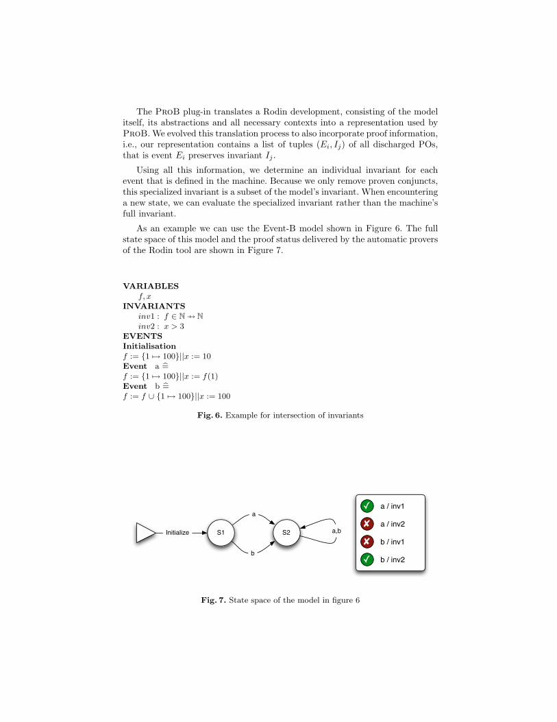
The ProB plug-in translates a Rodin development, consisting of the modelitself, its abstractions and all necessary contexts into a representation used byProB. We evolved this translation process to also incorporate proof information,i.e., our representation contains a list of tuples (Ei, Ij) of all discharged POs,that is event Ei preserves invariant Ij .
Using all this information, we determine an individual invariant for eachevent that is defined in the machine. Because we only remove proven conjuncts,this specialized invariant is a subset of the model’s invariant. When encounteringa new state, we can evaluate the specialized invariant rather than the machine’sfull invariant.
As an example we can use the Event-B model shown in Figure 6. The fullstate space of this model and the proof status delivered by the automatic proversof the Rodin tool are shown in Figure 7.
VARIABLESf, x
INVARIANTSinv1 : f ∈ N 7→ Ninv2 : x > 3
EVENTSInitialisationf := {1 7→ 100}||x := 10Event a b=f := {1 7→ 100}||x := f(1)Event b b=f := f ∪ {1 7→ 100}||x := 100
Fig. 6. Example for intersection of invariants
S1 S2
a
b
a,bInitialize
✓
✓
✘
✘
a / inv1
a / inv2
b / inv1
b / inv2
Fig. 7. State space of the model in figure 6

The proof status at the right shows, that Rodin is able to discharge theproof obligations a/inv1 and b/inv2 but not a/inv2 and b/inv1. This means, ifa occurs, we can be sure that f ∈ N 7→N holds in the successor state if it holds inthe predecessor state. Analogously, we know, that if b occurs, we are sure, thatx > 3 holds in the successor state if it holds in the predecessor state.
Consider a situation, where we already verified that all invariants hold forS1 and we are about to check S2 is consistent. We discovered two incomingtransitions corresponding to the events a and b. From a, we can deduct thatf ∈ N 7→ N holds. From b, we know that x > 3 holds. To verify S2, we need tocheck the intersection of unproven invariants, i.e., {f ∈ N 7→ N} ∩ {x > 3} = ∅,thus we already know that all invariants hold for S2.
This is of course only a tiny example but it demonstrates, that using proofinformation we are able to reduce the number of invariants for each event sig-nificantly, and sometimes by combining proof information from different events,we are able to get rid of the whole invariant. We actually have evidence that thisis not only a theoretical possibility, but happens in real world specifications (seeSection 7.2).
Algorithm 8 describes ProB’s consistency checking algorithm, we will justifyit formally in section 6.1. The algorithm employs a standard queue data structureto store the unexplored nodes. The key operations are:
– Computing the successor states, i.e., “state →evt succ”.– Verification of the invariant “∃invi ∈ Inv(state) s.t . invi is false”– Determining whether “succ 6∈ Visited”
The algorithm terminates when there are no further queued states to ex-plore or when an error state is discovered. The underlined parts highlight theimportant differences with the algorithm in [38].
In contrast to the algorithm, the actual implementation does the calculationof the intersection (Inv(succ) := Inv(succ) ∩ Unproven(op)) in a lazy manner,i.e., for each state 6∈ V isited, we store the event names as a list. As soon aswe evaluate the invariant of a state, we calculate and evaluate the intersectionon the fly. The reason is, that storing the invariant’s predicate for each state istypically more expensive than storing the event names.
Verification To show, that our approach is indeed correct, we developed aformal model of an abstraction of algorithm 8. We omitted few technical de-tails, such as the way the state space is traversed by the actual implemen-tation and also we omitted the fact, that our implementation always uses allavailable information. Instead, we have proven correctness for any traversaland any subset of the available information. Our model was developed usingEvent-B and fully proven in Rodin. The model is available as a Rodin 1.0archive from http://deploy-eprints.ecs.soton.ac.uk/152/. In this reportwe present only some parts of the model and some lemmas, without their proofs.All the proofs can be found in the file, we thus refer the reader to the Rodinmodel.
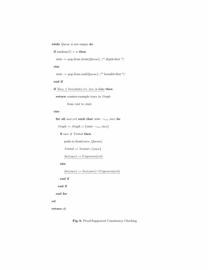
while Queue is not empty do
if random(1) < α then
state := pop from front(Queue); /* depth-first */
else
state := pop from end(Queue); /* breadth-first */
end if
if ∃invi ∈ Inv(state) s.t. invi is false then
return counter-example trace in Graph
from root to state
else
for all succ,evt such that state →evt succ do
Graph := Graph ∪ {state →evt succ}
if succ 6∈ Visited then
push to front(succ, Queue);
Visited := Visited ∪ {succ}
Inv(succ) := Unproven(evt)
else
Inv(succ) := Inv(succ) ∩ Unproven(evt)
end if
end if
end for
od
return ok
Fig. 8. Proof-Supported Consistency Checking

We used three carrier sets STATES, INVARIANTS and EVENTS. We as-sume, that these sets are finite. For invariants and events this is true by definitionin Event-B, but the state space can in general be unbounded. However, the as-sumption of only dealing with finite state spaces is reasonable in the context ofour particular model, because we can interpret the STATES set as the subset ofall states that can be traversed by the model checker within some finite numberof steps.9 The following definitions are used to prove some properties of Event-B:
truth ⊆ STATES× INVARIANTStrans ⊆ STATES× STATESpreserve = {s | {s} × INVARIANTS ⊆ truth}violate = STATES \ preservelabel ⊆ trans× EVENTSdischarged ⊆ EVENTS× INVARIANTS
The model also contains a set truth: pair of a state s and an invariant i is intruth if and only if i holds in s. The set preserve is defined as the set of stateswhere each invariant holds, the relations trans and label describe, how two statesare related, i.e. a triple (s 7→ t) 7→ e is in label (and therefore s 7→ t ∈ trans) ifand only if t can be reached from s by executing e. The observation that is thefoundation of all theorems we proved and is the following assumption:
∀i, t · (∃s, e · s ∈ preserve ∧ (s 7→ t) ∈ trans∧
(s 7→ t) 7→ e ∈ label ∧ (e 7→ i) ∈ discharged)
⇒ (t 7→ i) ∈ truth
The assumption is, that if we reach a state t from a state s where all invariantshold by executing an event e and we know, that the invariant i is preserved by e,we an be sure, that i holds in t. This statement is what we prove by dischargingan invariant proof obligation in Event-B, thus it is reasonable to assume that itholds.
We are now able to prove a lemma, that will capture the essence of ourproposal; it is enough to find for each invariant i one event that preserves thisinvariant leading from a consistent state into a state t to prove, that all invariantshold in t.
Lemma 1. ∀t · t ∈ STATES∧ (∀i · i ∈ INVARIANTS∧ (∃s, e · s ∈ preserve∧ e ∈EVENTS ∧ (s 7→ t) ∈ trans ∧ (s 7→ t) 7→ e ∈ label ∧ e 7→ i ∈ discharged)) ⇒ t ∈preserve
Proof. All proofs have been done using Rodin and can be found in the modelarchive. ut9 Alternatively, we can remove this assumption from our Rodin models. This only
means that we are not be able to prove termination of our algorithm; all otherinvariants and proofs remain unchanged.

We used five refinement steps to prove correctness of our algorithm. Wewill describe the first three steps, the last two steps are introduced to provetermination of new events. The first refinement step mc0 contains two eventscheck state ok and check state broken. The events take a yet unprocessed stateand move it either into a set containing consistent or inconsistent states. Al-gorithm 9 shows the check state ok event, check state broken is defined analo-gously, except that it has the guard s 6∈ preserve and it puts the state into theset inv broken.
event check state ok
any s
where
s ∈ open
s ∈ preserve
then
inv ok := inv ok ∪ {s}
open := open \ {s}
end
Fig. 9. Event check state ok from mc0
At this very abstract level this machine specifies that our algorithm separatesthe states into two sets. If they belong to preserve, the states are moved into theset inv ok . Otherwise, they are moved into inv broken. Lemma 2 guarantees,that our model always generate correct results.
Lemma 2. mc0 satisfies the invariants
1. inv ok ∪ inv broken = STATES \ open2. open = ∅⇒ inv ok = preserve ∧ inv broken = violate
The next refinement strengthens the guard and removes the explicit knowl-edge of the sets preserve and violate, the resulting proof obligation leads tolemma 3.
Lemma 3. For all s ∈ open
{s} × INVARIANTS \ discharged[label[inv ok C trans B {s}]]) ⊆ truth
⇔ s ∈ preserve

The third refinement introduces the algorithm. We introduce a new relationinvs to verify in this refinement. The relation keeps track of those invariants,that need to be checked, in the initialization, we set invs to verify := STATES×INVARIANTS.
The algorithm has three different phases. It first selects a state that has notbeen processed yet then it checks if the invariant holds and moves the state intoeither inv ok or inv broken. Finally, it uses the information about dischargedproofs to remove some elements from invs to verify as shown in algorithm 10.
event mark successor
any p s e
where
p ∈ inv ok
s ∈ trans[{p}]
(p 7→ s) 7→ e ∈ label
(p 7→ s) 7→ e 6∈ marked
ctrl = mark
then
invs to verify := invs to verify �− ({s}× (invs to verify [{s}]∩ unproven[{e}]))
marked := marked ∪ {(p 7→ s) 7→ e}
end
Fig. 10. Event mark successor from mc2
We take some state s and event e, where we know that s is reachable via efrom a state p, where all invariants hold. Then we remove all invariants but those,that are not proven to be preserved by e. This corresponds to the calculation ofthe intersection in algorithm 8.
The main differences between the formal model and our implementation are,that the model does not explicitly describe how the states are chosen and thealgorithm uses all available proof information while the formal model can use anysubset. In addition, the model does not stop if it detects an invariant violation.We did not specify these details because it causes technical difficulties (e.g., we

need the transitive closure of the trans relation) but does not seem to provideenough extra benefit.
Correctness of algorithm 8 is established by the fact that the outgoing edgesof a state are added to the Graph only after the invariants have been checked forstate. Hence, the removal of a preserved invariant only occurs after it has beenestablished that the invariant is true before applying the event. This correspondsto the guard p ∈ inv ok . However, the proven proof obligations for an eventonly guarantee preservation of a particular invariant, not that this invariant isestablished by the event. Hence, if the invariant is false before applying the event,it could be false after the event, even if the corresponding proof obligation isproven and true. If one is not careful, one could easily set up cyclic dependenciesand our algorithm would incorrectly infer that an incorrect model is correct.
Proof-Assisted Consistency Checking for Classical-B In the setting ofEvent-B and the Rodin platform, ProB can rely on the other tools for providingtype inference and as we have seen the proof information.
In the context of classical B, we are working on a tighter integration withAtelier B [54]. However, at the moment ProB does not have access to the proofinformation of classical B models.
ProB does perform some additional analyses of the model and annotates theAST (Abstract Syntax Tree) with additional information. For instance for eachevent we calculate a set of variables that are possibly modified. For instance ifwe analyze the operation10
Operation1 = BEGIN x := z || y := y ∧ {x 7→ z} END
the analysis will discover that the set of variables that could potentially influencethe truth value of the invariant is {x, y}.
This analysis was originally used to verify the correct usage of SEES in theclassical B-Method. The SEES construct was used in the predecessor of Event-B,so-called classical B, to structure different models. In classical B a machine cansee another machine, i.e., it is allowed to call operations that do not modifythe state of the other machine. To support this behavior, it was necessary toknow if an operation has effect on state variables, that is the set of modifiedvariables is the empty set. It turned out, that the information is more valuablethan originally thought, as it is equivalent to some proof obligation:
If u and v are disjoint sets of state variables, and the substitution of an oper-ation is SBA(v, t, v′) we know that u = u′ and thus a simplified proof obligationfor the preservation of an invariant I(u) over the variables u is
I(u) ∧G(u ∪ v, t) ∧ SBA(v, t, v′)⇒ I(u)
which is obviously true. These kind of proof obligations are not generated byany of the proving environments for B we are aware of. In particular Rodin does
10 Operations are the equivalent of events in classical B.

not generate them. For a proving environment, this is a good idea as they do notcontain valuable information for the user and they can be filtered out by simplesyntax analysis. But for the model checker these proofs are very valuable; in mostcases they allow us to reduce the number of invariants we need to check. As thistype of proof information can be created from the syntax, we can use them evenif we do not get proof information from Rodin, i.e., when working on classical Bmachines. As such, we were able to use Algorithm 8 also for classical B modelsand also obtain improvements of the model checking performance (although lessimpressive than for Event-B).
Conclusion and Future Work First of all, we never found a model whereusing proof information significantly reduced the performance, i.e., the additionalcosts for calculating individual invariants for each state are rather low. Usingproof information is the new default setting in ProB.
We got a number of models, in particular those coming from industry, whereusing the proof information has a high impact on the model checking time. Inother cases, we gained only a bit or no improvement. This typically happens ifthe invariant is rather cheap to evaluate compared to the costs of calculating theguards of the events. We used an out-of-the-box version of Rodin11 to produceour experimental results. Obviously, it is possible to further improve them byadding manual proof effort. In particular, it gives the user a chance to influ-ence the speed of the model checker by proving invariant preservation for thoseparts that are difficult to evaluate, i.e., those predicates that need some kind ofenumeration.
Related Work A similar kind of integration of theorem proving into a modelchecker was previously described in [?]. In their work Pnueli and Shahar intro-duced a system to verfify CTL and LTL properties. This system works as a layeron top of CMU SMV and was sucessfully applied to fragments of the Futurebus+system [?]. SAL is a framework and tool to combine different symbolic analysis[52], and can also be viewed as an integration of theorem proving and modelchecking. Mocha [5] is another work where a model checker is complemented byproof, mostly for assume-guarantee reasoning. Some more works using theoremproving and model checking together are [20, 7, 21, 26].
In the context of B, the idea of using a model checker to assist a prover hasalready been exploited in practice. For example, in previous work [11] we havealready shown how a model checker can be used to complement the provingenvironment, by acting as a disprover. In [11] it was also shown that sometimesthe model checker can be used as a prover, namely when the underlying setsof the proof obligation are finite. This is for example the case for the vehiclefunction mentioned in [36]. Another example is the Hamming encoder in [18],where Dominique Cansell has used ProB to prove certain theorems which aredifficult to prove with a classical prover (due to the large number of cases).
11 For legal reasons, it is necessary to install the provers separately

Future Work We have done but a first step towards exploiting the full poten-tial for integrating proving and model checking. For instance, we may feed thetheorem prover with proof obligations generated by the model checker in orderto speed up the model checking. A reasonable amount of time is spent evaluatingthe guards. If the model checker can use the theorem prover to prove that anevent e is guaranteed to be disabled after an event f occurs, we can reduce theeffort of checking guards. We may need to develop heuristics to find out whenthe model checker should try to get help from the provers.
Also we might feed information from the model checker back into the provingenvironment. If the state space is finite and we traverse all states, we can use thisas a proof for invariant preservation. ProB restricts all sets to finite sets [38]to overcome the undecidability of B, so this needs to be handled with care. Weneed to ensure, that we do not miss states because ProB restricted some sets.Also we need to ensure that all states are reachable by the model checker, thuswe may need some additional analysis of the model.
We also think of integrating a prover for classical B, to exploit proof infor-mation. The integration is most likely not as seamless as in Rodin and the costsof getting proof information is higher.
Although the cost of calculating the intersections of the invariants for eachstate is too low to measure it, the stored invariants take some memory. It mightbe possible to find a more efficient way to represent the intersections of invariants.

6.2 Automatic Flow Analysis
Event-B [3] has only very limited ways to express ordering of events. In particularit lacks a notion of sequential composition, or other ways to explicitly describethe ordering of events. If we specify software or systems that include software inEvent-B, we often have some implicit algorithmic structure.12 Unfortunately thisinformation is implicit only and therefor not directly usable by tools nor directlyvisible to users. We report on a method to uncover this implicit algorithmicstructure. This information can be useful for analyzing or comprehending modelsand for automatic code generation. We also show how to use this information toimprove model checking. We use Event-B to illustrate our approach and presentan implementation for Event-B inside the animator an model checker ProB.Our method, however, is not limited to that particular specification languageand can also be used for a range of other formalisms such as TLA+.
Preliminaries We follow the style of [3] of expressing variables and substitutionin formulas. In particular, let v = v1, . . . , vn be a sequence of n distinct variables,t = t1, . . . , tn a sequence of n formulas and F a formula. Then F [t/v] is obtainedfrom F by replacing simultaneously all free occurrences of each vi by ti. Welet F (v) denote a formula, whose free variables are among v1, . . . , vn. Once theformula F (v) has been introduced, we denote by F (t) the formula F [t/v] withv replaced by t.
In Event-B a state consists of a set of variables that are modified by events.The values of the variables are constrained by invariants I(v). Each event iscomposed of a guard G(t, v) and an action S(t, v), where t are parameters of theevent. We will only consider events of the form
evt = any twhen G(t, v)then vi1 , . . . , vik
:= E1(v, t), . . . , Ek(v, t) end
for some ij ∈ i1, . . . , in. Note that t can be empty and G(t, v) can be true.Also note that k can be 0, in which case we write the action part as skip.
All assignments of an action S(t, v) occur simultaneously. Variables vj1 , . . . , vjl
that do not appear on the left-hand side of an assignment of an action are notchanged by the action. The effect of an assignment can be described by a before-after predicate:
S(v, t, v′) = v′i1 = E1(v, t) ∧ . . . v′ik= Ek(v, t) ∧ v′j1 = vj1 ∧ . . . v′jl
= vjl
A before-after predicate describes the relationship between the state just be-fore an assignment has occurred, x, and the state just after the assignment hasoccurred, x′.
12 To order events in Event-B the usual method is to introduce abstract program coun-ters.

Note that Event-B also allows non-deterministic actions of the form x :∈E(t, v) or x :| Q(t, v, x′). To simplify the presentation of our method, and with-out loss of generality, we assume that those are rewritten to the above formusing new parameters, one for every non-deterministic action which denotes thechosen element. For instance, we rewrite
any max when max > 10 then x :∈ 1..max end
into
any max, choice when max > 10 ∧ choice : 1..max then x := choice end
Dependency Between Events We are interested in how events influenceeach other. The motivations are multiple: either we may try to understand thedynamic behavior of our model, we may wish to generate code by determiningthe control flow or we may wish to improve the performance of model checking...
Suppose we have an event g with action x, y := x + 1, 0. There are variousways it can influence another event:
1. it can disable another event. E.g., the event h with guard y > 0 will for surebe disabled after executing g.
2. it can enable another event. E.g., the event h′ with guard y = 0 would forsure be enabled after executing g.
3. it can be independent of another event. For example, the enabling of theevent h′′ with guard z > 0 would not be modified by executing g, i.e., it willbe enabled after g if and only if it was enabled before. (Note that, dependingon the action part of h′′, the effect of h′′ could have been modified.)
In cases 1 and 2 the enabling or disabling may depend on the current stateof the model. Take for example the event h′′′ with guard y = 0 ∧ x > 1. Thenh′′′ would be enabled after g if x > 0 holds in the state before executing g, anddisabled otherwise. The predicate x > 0 is what we call an enabling predicate,and which we define as follows:
Definition 1 (Enabling predicate). The predicate P is called enabling pred-icate for an event h after an event g, denoted by g ;P (v,t,s) h, if and only if thefollowing holds
I(v) ∧G(v, t) ∧ S(v, t, v′)⇒ (P (v, t, s)⇔ H(v′, s))
where I(v) is the invariant of the machine, G(v, t) is the guard of g with pa-rameters t and S(v, t, v′) the before-after predicate of its action part, and whereH(v, s) is the guard of h with parameters s.
In the absence of non-deterministic actions, an equivalent definition can beobtained using the weakest precondition notation:
I(v) ∧G(v, t)⇒ (P (v, t, s)⇔ [S(t, v)]H(v, s))

where [S]P denotes the weakest precondition which ensures that after executingthe action S the predicate P holds.
Note that it is important for us that the action part S(t, v) of an event doesnot contain any non-determinism (i.e., that all non-determinism has been liftedto the parameters t; see Section 6.2). Indeed, in the absence of non-determinism,the negation of an enabling predicate is a disabling predicate, i.e., it guaranteesthat the event h is disabled after g if it holds (together with the invariant) beforeexecuting g. However, if we have non-determinism the situation is different.There may even exist no solution for P (v, t, s) in Def. 1, as the following exampleshows.
Example 1. Take x :∈ {1, 2} as the action part of an event g with no parametersand the guard true and x = 1 as the guard of h. Then [S(t, v)]H(v) ≡ falseas there is no way to guarantee that h is enabled after g. Indeed, there is nopredicate over x that is equivalent to x′ = 1 in the context Def. 1 : the before afterpredicate S(v, t, v′) is x′ ∈ {1, 2} and does not link x and x′. Similarly, there is noway to guarantee that h is disabled after g. In particular, ¬[S(t, v)]H(v) ≡ trueis not a disabling predicate.
Note that if I(v) ∧G(v) ∧ [S(t, v)]H(v, s) is inconsistent, then any predicateP (v, t, s) is an enabling predicate, i.e., in particular P (v, t, s) ≡ false.
How can we compute enabling predicates? Obviously, [S(t, v)]H(v) alwayssatisfies the definition of an enabling predicate. What we can do, is simplify itin the context of I(v)∧G(v).13 We will explain later in Sect. 6.2 exactly how wecompute enabling predicates.
Example 2. Take for instance a model of a for loop that iterates over an arrayand increments each value by one. Assuming the array is modeled as a functionf : 0..n → N and we have a global counter i : 0..(n + 1), we can model the forloop (at a certain refinement level) using two events terminate and loop.
terminate = when i > n then skip end
loop = when i ≤ n then f(i) := f(i) + 1||i := i+ 1 end
We can now try to find enabling predicates for each possible combination ofevents. Table 9 shows the proof obligations from Def. 1 and simplified predicatesP which satisfy it.
The directed graph on the left in Figure 11 is a graphical representation ofTable 9. Every event is represented by a node and there for every enabling pred-icate first;P second from Table 9 there is an edge between the correspondingnodes.
The right picture shows the same graph if we take independence of eventsinto account, i.e., if an event g cannot change the guard of another event h, we13 This is similar to equivalence preserving rewriting steps within sequent calculus
proofs, where I(v), G(v) are the hypothesis and [S(t, v)]H(v) is the goal of the se-quent.

Event Pairs (first ;P second) Enable Predicate Definition (wp notation) Simplified P
terminate ;P terminate i > n =⇒ (P ⇐⇒ i > n) trueloop ;P loop i ≤ n =⇒ (P ⇐⇒ (i+ 1) ≤ n) (i+ 1) ≤ nloop ;P terminate i ≤ n =⇒ (P ⇐⇒ (i+ 1) > n) (i+ 1) > nterminate ;P loop i > n =⇒ (P ⇐⇒ i ≤ n) false
Table 9. Enable Predicates for a simple model
do not insert an edge between g and h. In particular, as terminate does notmodify any variables, it cannot modify the truth value of any guard. On firstsight it seems as if we may have also lost some information, namely that afterthe execution of terminate the event loop is certainly disabled. We will returnto this issue later and show that for the purpose of reducing model checking andother application, this is actually not relevant.
terminate loop
(i+1) > n
false
(i+1) ≤ ntrue terminate loop
(i+1) > n
(i+1) ≤ n
Fig. 11. Graph Representations of Dependence for a Simple Model
In Event-B models of software components independence between events oc-curs very often, e.g., if an abstract program counter is used to activate a specificsubset of the events at a certain point in the computation. We can formallydefine independence as follows.
Definition 2 (Independence of events). Let g and h be events. We say thath is independent from g — denoted by g 6; h — if the guard of h is invariantunder the substitution of g, i.e., iff the following holds:
I(v) ∧G(v, t) ∧ S(v, t, v′) =⇒ (H(v, s) ⇐⇒ H(v′, s))
Our first observation is that an event g can only influence the enablednessof an event h (we do not require g 6= h) if g modifies some variables that areread in the guard of h. We denote the set of variables used in the guard of hby read(h) and the set of variables modified by g by write(g). If write(g) andread(h) are disjoint, then h is trivially independent from g:
Lemma 4. For any two events h and g we have that read(h) ∩ write(g) = ∅⇒ g 6; h.
This happens in our loop example, because read(terminate) = ∅, and henceall events (including terminate itself) are independent from terminate.
However, read(h) ∩ write(g) = ∅ is sufficient for independence of eventsbut not necessary. Take for instance the events from figure 12. Event g clearlymodifies variables that are read by h and therefor read(h)∩write(g) 6= ∅ but gcan not enable or disable h.
event g event h
begin when
x := x + 1 x + y > 5
y := y - 1 then
end end
Fig. 12. Independent events
The trivial independence can be decided by simple static analysis, i.e., bychecking if read(h) ∩ write(g) = ∅. Non trivial independence is in general un-decidable. In practice, it is a good idea to try to prove that two events areindependent in the sense of Def. 2, as it will result in a graph representationwith fewer edges. However, it is not crucial for our method that we detect allindependent events.
As we have seen in the right side of Fig. 11, the information we gain aboutenabling and independence can be represented as a directed graph, now formallydefined as follows.
Definition 3 (Enable Graph). An Enable Graph for an Event-B model isa directed edge labeled graph G = (V,E,L). The vertices V of the graph arethe events of the model. Two events can be linked by an edge if they are notindependent, i.e., (g 7→ h) 6∈ E ⇒ g 6; h. Each existing edge g 7→ h is labeledwith the enabling predicate, i.e., g ;L(g 7→h) h.
Above we define a family of enable graphs, depending on how precise ourinformation about independence is. Below, we often talk about the enable graphfor a model, where we assume a fixed procedure for computing independenceinformation.
Aside. There is another representation of the graph that is sometimes moreconvenient for human readers. We can represent the graph as a forest where eachtree has one event as its root and only the successor nodes as leafs. The alternaterepresentation is shown in figure 13 for a small example.
Computing the Enabling Predicates As mentioned in section 6.2, the weak-est precondition [S(t, v)]H(v, t, s) obviously satisfies the property of enablingpredicates. We can use the syntax tree library of the Rodin tool to calculate theweakest precondition. However, these candidates for enabling predicates need tobe simplified, otherwise they are as complicated as the original guard and we willgain no benefit from them. therefor we simplify the candidate, in the context ofthe invariant I(v) and the guard of the preceding event G(v, t).

a
c
b aPQ
true false
b c
trueQ
b
a c
falsep
c
Fig. 13. Representations of the Enable Graph
Consider the model shown in figure 6.2. The weakest precondition for g pre-ceding h is [x := x+ 2]x = 1 which yields x = −1. This contradicts the invariantx > 0 and thus h can never be executed after g took place. In the context of theinvariant, x = −1 is equivalent to false.
invariant x > 0
event g event h
begin when x = 1
x := x + 2 end
end
Fig. 14. Simplification
The simplification of the predicates is an important step in our method, deriv-ing an enabling predicate P (v, t, s) from the weakest precondition [S(t, v)]H(v, s).Recall, that we simplify the predicate [S(t, v)]H(v, s) in the context of the in-variant I(v) (and the guard G(v, t))
I(v) ∧G(v, t)⇒ (P (v, t, s)⇔ [S(t, v)]H(v, s))
A very important requirement in our setting is that the simplifier never in-creases the number of conjuncts. We have to keep the input for our enable andflow graph constructions small to prevent exponential blowup. Our simplifiershall find out if a conjunct is equivalent to true or false. In the first case the con-junct can be removed from the predicate in the second case the whole predicateis equivalent to false.
We have implemented a first prototype simplifier in Prolog that uses a rel-atively simple approach. The core algorithm is presented in Fig. 15. First itnormalizes all negated formulas; this is part of the conjuncts function, whichalso translates the formula into a set of conjuncts. For example, the formulax 6= false is normalized to x = true and ¬(a ≤ b) is normalized to a > b.Then we successively try to add the conjuncts of the formulas to a set of currentconjuncts K. If we try to add the conjunct C we can observe two special cases:
1. c is already a member of K: then we skip c because we know that it is truein the context of K.

KI := closure(conjuncts(I(v))) (is precomputed)Kg := closure(conjuncts(G(v, t))) (is precomputed for every event g)K := closure(KI ∪Kg)WP := conjuncts([S(t, v)]H(v, s))P := ∅while WP 6= emptyset do
choose C and remove from WPif C 6∈ K thenK := closure(K ∪ {C})if inconsistent(K) thenP := {false}; WP := ∅
elseP := P ∪ {C}
end ifend if
odP is the simplified version of [S(t, v)]H(v, s)
Fig. 15. Algorithm for simplifying the weakest precondition in the context of the in-variant and guard of g
2. c is inconsistent with a member of K: then the enabling predicate is false.
The second special case is detected using a few number of Prolog clauses such asthe following (where, the first argument is the binary operator followed by thearguments to the operator):
inconsistent_fact(not_equal,X,X).
inconsistent_fact(less,X,X).
inconsistent_fact(less,X,Y) :- value(X), value(Y), X >= Y.
inconsistent_fact(equal,X,Y) :- value(X), value(Y), X \= Y.
inconsistent_fact(member,_,empty_set).
% some more rules [...]
The first rule states that x 6= x is inconsistent, the second one that x < x isinconsistent, the third one that x < y is inconsistent if x and y are known valueswith x ≥ y, and so on.
In any other case we add the conjunct and calculate the closure of K usingsome rules that combine two formulas, computing new logical consequences (e.g.,deriving from transitivity of the arithmetic operators, i.e., x ≤ y and y < zimplies x < z).
For example, assume we have built the set of conjuncts K = {x < 2, y = 5}and we now try to add x = y. Combining x = y with y = 5 yields x = 5 whichwe add to K.
Assume we have only the rules mentioned above. Now we combine x = 5 andx < 2, yielding the new fact 5 < 2. This triggers the third Prolog rule detectingan inconsistency.
The actual implementation does not always recompute everything from scratch.As outlined in algorithm 15 we precompute a closure KI from the conjuncts of

the invariant. This set can be reused for the whole model. For each event g weprecompute a closure Kg from the guards. This set can be reused for all enablingpredicates where g is the first event.If the algorithm has not stopped because ofa contradiction the enabling predicate is the conjunction of the formulas storedin P .
Using the Enable Graph for Model Checking The enable graph containsvaluable information for a model checker. In this section we describe how it canbe used within ProB. When checking the consistency of an Event-B model,ProB traverses the state space of the model starting from the initialization andchecks the model’s invariant for each state it encounters. The cost for checkinga state is the sum of the cost of evaluating the invariant for the state and thecalculation of the successors. Finding successor states requires to find solutionsfor the guards of each event. A solution means that the event is applicable andwe can find some parameter values. ProB then applies the actions to the currentstate using the parameter values resulting in some successor states. In some casesthe enable graph can be used to predict the outcome of the guard evaluation.The special case of an enabling predicate P = false is very important. It meansthat no matter how we invoke g we can omit the evaluation of the guard of hbecause it will be false after observing g. In other words it is a proof that theproperty h is disabled holds in any state that is reachable using g.
When encountering a new state s via event e, we look up e in the enablegraph. We can safely skip evaluation of the guards of all events f that have anedge (e,f) which is labeled with false in the Enabled Graph. We can even goa step further if we have multiple ways to reach s. When considering an eventto calculate successor states we can arbitrary chose one of the incoming eventsand use the information from the enable graph. For instance, if we have fourevents a, b, c and d and we know that a disables c and b disables d. Furthermorewe encounter a state s via a but do not yet calculate the successors. Later weencounter s again, this time via b. When calculating the successors we can skipboth, c and d.
The reason is that we have a proof for c is disabled because the state wasreachable using event a and a proof that d is disabled because the state wasreachable using event b. Thus the conjunction c and d are disabled is also true.
Because we use the invariant when simplifying the enabling predicate (seeSection 6.2), the invariant must hold in the previous state in order to use theflow information. However we believe this is reasonable because most of the timewe are hunting bugs and thus we stop at a state that violates the invariant. Theimplementation must take this into account and in case of an invariant violationit must not use the information gained by flow analysis. Also it needs to checknot only the invariant but also the theorems if they are used in the simplifier.
Enable Graph Case study In this section, we will apply the concept to amodel of the extended GCD algorithm taken from [27]. The model consists ofa refinement chain, where the last model consists of two loops. The first loop

builds a stack of divisions. The second loop calculates the result from this stack.The last refinement level contains five events excluding the initialization. Theevents up and dn are the loop bodies, the events upini, dnini initialize the loopsand gcd is the end of the computation. The event init is the INITIALISATIONof the model.
gcd
init
true
falsefalse
false
false
upini
false
dn=false & a mod b != 0 dn = true
dn=false & a mod b = 0
false
up
t(f) mod r(f) != 0
false
t(f) mod r(f) = 0
false
false dnini false
f > 0
false
f-1 = 0
falsedn
f-1 > 0
f = 0
Fig. 16. Enable graph of the extended GCD example
The first step is to extract the read and write sets for each event; the result isshown in Table 10. Then we construct the enable graph. We calculate the weakestprecondition for each pair of independent events and simplified them. Both stepswere done manually but they were not very difficult. For instance, the mostcomplicated weakest precondition was [Sup]Gdnini. In the presentation belowwe left out all parts of the guard and substitution that do not contain sharedidentifiers, e.g., the guard contains up = TRUE but the substitution does notmodify up. The next step is calculating the weakest precondition mechanically,finally we simplify the relational override using the rule (r �− a 7→ b)(a) = b.

event read(event) write(event)
init ∅ {a, b, d, u, v, up, f, s, t, q, r, uk, vk, dn, dk}upini {up} {up, f, s, t, q, r}up {up, r, f, dn} {f, s, t, r, q}gcd {up, f, dn} {d, u, v}dnini {up, dn, r, f} {dn, dk, uk, vk}dn {dn, f} {uk, vk, f}
Table 10. Read and write sets
[Sup]Gdnini = [f := f + 1, r �− {f + 1 7→ f(t) mod r(f)}] (r(f) = 0)= (r �− {f + 1 7→ t(f) mod r(f)})(f + 1) = 0
= t(f) mod r(f) = 0
The other simplification were much easier, for example, replacing dn =TRUE ∧ dn = FALSE by false. The constructed graph is shown in figure 16.
The enable graph can be used by the model checker to reduce the number ofguard evaluations. Let us examine one particular run of the algorithm for fixedinput numbers. The run will start with init and upini then contain a certainnumber of up events, say n. This will be followed by dnini and then exactly ndn events and will finish with one gcd event. In all, the calculation takes 2n+ 4steps. After each step, the model checker needs to evaluate 5 event guards (onefor each event, except for the guard of the initialization which does not need tobe evaluated) yielding 10n+20 guard evaluations in total. Using the informationof the enable graph we only need a total of 4n+4 guard evaluations. For example,after observing up, we only need to check the guards of up and dnini: they arethe only outgoing edges of up in Fig. 16 which are not labelled by false.
Flow Construction Beside the direct use in ProB the enable graph can beused to construct a flow. A flow is an abstraction of the model’s state spacewhere an abstract state represents a set of concrete states. Each abstract stateis characterized by a set of events, representing all those concrete states wherethose (and only those) events are enabled.
The flow graph is a graph where the vertices are labeled with sets of events,i.e., the set of enabled events. The edges are labeled with an event and a predicatecomposed from the enable predicates for this event. The construction of the flowgraph takes the enable graph as its input. Starting from the state where only theinitialization event is enabled the algorithm unfolds the enable graph. We willdescribe the unfolding in a simple example, an algorithm is shown in Figure 18and 19.
Figure 17 shows a simple flow graph construction. On the left side the enablegraph for the events init, a and b are shown. The graph reveals that b alwaysdisables itself while it does not change the enabledness of a. The event a keeps

itself enabled if and only if P holds and it enables b if and only if Q holds. Theinit event enables a and disables b.
We start the unfolding in the state labeled with {init}. In this case we donot have a choice but to execute init. From the enable graph on the left handside we know that after init occurs a is the only enabled event. Therefor wehave to execute a. We know that if P is true then a will be enabled afterwardsand analogously if Q holds then b will be enabled. Combining all combinationof P and Q and their negations, we get the new states {}, {b} and {a, b}. If wecontinue, we finally get the graph shown on the right hand side. If more thanone event is enabled, we add edges for each event separately. We can combineedges by disjunction of the predicates. In our case we did that for the transitionfrom {a, b} to {a} which can be used by either executing b or a.
The algorithm in Figure 19 calculates for a given event e the successors inthe flow graph by combining all possible configurations. The algorithm also usesa list of independent events that are enabled in the current state and thereforthey are also enabled in any new state. The algorithm in Figure 18 produces theflow graph starting form the state {init}.
a
ba
P Q
b
b
false {a}
{}
{b}
{a,b}
(a,¬P∧¬Q)
(a,¬P∧Q)
(a,P∧Q)
(a,P∧¬Q)
(a,P∧¬Q) ∨
(b,true)
(a,¬P∧Q)
(a,¬P∧¬Q)(b,true)
Fig. 17. Simple Flow Graph Construction
Generating the Flow Graph can be infeasible because the graph can be of sizeO(2#Events). However, in cases where constructing the flow graph is feasible, wegain a lot of information about the algorithmic structure and we can generatecode if the model is deterministic enough. We will discuss applicability andrestrictions of the methods in section 6.2.
Flow Graph Case Study If we apply the flow construction to the examplegraph shown in figure 16 we get the flow graph shown in figure 21. Compared

todo := {{init}}done := ∅flow := ∅while todo 6= emptyset do
choose node from todoforeach e ∈ node dokeep := node ∩ independent(e)atoms := expand(e, keep)todo := (todo ∪ ran(atoms))flow := flow ∪ {node 7→ atoms}
oddone := done ∪ {node}todo := todo− done
od
Fig. 18. Algorithm for constructing a Flow Graph
Given: enable graph as EG : (Events× Events) 7→ Predicatedef expand(e, keep) =true pred := {f 7→ true|(e 7→ f) ∈ dom(EG) ∧ EG(e 7→ f) = true}maybe pred := {f 7→ p|(e 7→ f) ∈ dom(EG) ∧ EG(e 7→ f) = p ∧ p 6= false}result := ∅
foreach s ⊆ node dotargets := dom(true pred) ∪ dom(s) ∪ keeppredicate :=
Vran(s) ∧ ¬(
Wran(s�−maybe pred)
result := result ∪ {predicate 7→ targets}od
return resultend def
Fig. 19. Algorithm for expanding the Enable Graph (i.e., computing successor config-urations)

to the structured model developed by Hallerstede in [27] shown in 20 we see avery similar shape.
up
upini
dn
dnini gcd
Fig. 20. Structural model from [27]
However, the automatic flow analysis helped us to discover an interestingproperty. The flow graph contains a state that corresponds to concrete stateswhere no event is enabled, i.e., states where the system deadlocks. Thus themodel contains a potential deadlock. Inspection showed that the deadlock ac-tually does not occur. The reason why the flow graph contains the deadlockstate is a guard that is too strong. The guards of dn and gcd only cover f ≥ 0.The invariant implicitly prevents the system from deadlocking by restricting thevalues of f .
{dnini}{init}
{}
{upini}
{up} {dn}
{gcd}
true
a mod b ≠ 0
a mod b = 0
t(f) mod r(f) ≠ 0
t(f) mod r(f)
= 0
true
f > 0
f = 0
f < 0
f-1 > 0
f -1 = 0
f -1 < 0
Fig. 21. Example for a relation between abstract and concrete states
In Figure 21 we can see that is is possible to automatically generate sequentialcode from a flow graph. The events up and dn can be translated into while loopsand upini and dnini are if − then− else statements. In the particular case thetermination of the computation was encoded into the gcd event.

Applicability and Restrictions An important question is when to apply amethod and maybe even more important when not to apply it. It is clear that flowanalysis is probably not applicable if the model does not contain an algorithmicstructure. In the worst case for flow construction, any combination of events canbe enabled in some state, leading to 2card(Events) states, where card(Events) isthe number of events. However in case of software developments it is very likelythat eventually the model will contain events that are clustered, i.e, at each pointduring the computation a hopefully small set of events is enabled. We conjecturethat the more concrete a model is, the better are results from simplification.
Constructing the enable graph is relatively efficient; it requires to calculateO(card(Events)2) enabling predicates. In case of software specifications gener-ating the enable graph and using the information gained for guard reductionis probably worth trying. We can also influence the graph interactively. For in-stance, suppose the enable graph contains an edge labeled with card(x) > 0.Suppose we know that after the first event x = ∅ but the simplifier was tooweak to figure it out, i.e., the empty set is written down in a difficult way, let’ssay x := S∩T where S and T are disjoint. By specifying (and proving) a theoremthat helps the simplifier, e.g., x = ∅, we can interactively improve the graph.We believe that expressing these theorems does not only improve the graph butalso our understanding of a model because we explicitly formalize properties ofthe model that are not obvious (at least not for the automatic simplifier).
Constructing the flow graph is much more fragile; it can blow up very fast. Itis crucial to inspect the enable graph and try to reduce the size of the predicatesas much as possible. However our experience is that Event-B models of softwareat a sufficient low level of refinement typically have some notion of an abstractprogram counter that implicitly control the flow in a model. These abstractprogram counter are not very complicated and therefor it is likely that they areexploited by the simplifier.
Related and Future Work
Inferring Flow Information Model checking itself explores the state space ofa model, and as such infers very fine-grained flow information. For Event-B,the ProB model checker [36, 38] can be used for that purpose. However, it isquite rare that the complete state space of a model can be explored. When itis possible, the state space can be very large and flow information difficult toextract. Still, the work in [40] provides various algorithms to visualize the statespace in a condensed form. The signature merge algorithm from [40] merges allstates with the same signature, and as such will produce a picture very similarto the flow graph. However, the arcs are not labelled by predicates and theconstruction requires prior traversal of the state space.
Specifying Flow Information There is quite a lot of related work, where flowinformation is provided explicitly by the modeler (rather than being deducedautomatically, as in our method). For example, several works use CSP to specify

the sequencing of operations of B machines [55, 14, 16] or of Z specifications [22,42, 53, 8].
In the context of Event-B, there are mainly three other approaches that arerelated to our flow analysis. Hallerstede introduced in [27] a new approach tosupport refinement in Event-B that contains information about the structureof a component. Also Butler showed in [15] how structural information can bekept during refinement of a component. Both approaches have the advantage toincorporate the information about structure into the method, yielding in betterprecision. However both methods require the developer to use the methods fromthe beginning while automatic flow analysis can be applied to existing projects.In particular automatic flow analysis can actually be used to discover propertiesof a model such as liveness and feasibility of events. Hallerstede’s structuralrefinement approach does not fully replace our automatic flow analysis. Bothmethods overlap to some extend but we think that they can can be combined,such that the automatic flow analysis uses structural information to ease thegeneration of the flow graph and in return our method can suggest candidatesfor the intermediate predicates used during structural refinement. Actually theenable predicated can be used as candidates.
The third approach is yet unpublished but implemented as a plug-in forRodin [32]. It allows the developer to express flow properties for a model and toverify them using proofs.
Future Work The next step is to fully integrate our method into the next releaseof ProB, and use it to improve the model checking procedure and help the userin analyzing or comprehending models. We also plan to use the technique todevelop a new algorithm for test-case generation. In [56] we have introduce afirst test-case generation algorithm for Event-B, tailored towards event coverage.One issue is that quite often it is very difficult to cover certain events. Here theflow analysis will hopefully help guide the model checker towards enabling thosedifficult events.
Conclusion In summary, we have developed techniques to infer algorithmic struc-ture from a formal specification. From an Event-B model, we have derived theenable graph, which contains information about independence and dependenceof events. This graph can be used for model comprehension and to improvemodel checking. We have described a more sophisticated flow analysis, whichderives a flow graph from an Event-B model. It can again be used for modelcomprehension, model checking but also for code generation.

7 Workpackage I3: Parallel and Directed ProB
The techniques mentioned in Section 3.4 and Section 6.1 have been integratedinto the core ProB codebase and are now available in the latest distributions.The heuristic model checking algorithm has been integrated into the ProBcodebase, but is currently not available in the compiled versions (due to issuesgenerating a shared library version for the C++ priority queue under Windows).The implementation of the flow analysis from Section 6.2 is still ongoing. Be-low, we describe an empirical evaluation of the proof directed model checkingtechnique from Section 6.1.

7.1 Implementation and Evaluation of Proof-Directed MC
To show, that our approach is indeed correct, we developed a formal model of theAlgorithm used in ProB. The model was developed in Event-B and fully provenin Rodin. We have shown that the proof supported model checking algorithm isa refinement of the original algorithm. Thus the new algorithm accepts a stateif and only if the old one does.
7.2 Experimental results
To verify that the combination of proving and model checking results in a consid-erable reduction of model checking effort, we prepared an experiment consistingof specifications we got from academia and industry. The specification are takenfrom the benchmarks chosen in T1. In addition we prepared a constructed ex-ample as one case, where the prover has a very high impact on the performanceof the model checker. It basically contains an event, that increments a number xand an invariant ∀a, b, c.a ∈ N∧ b ∈ N∧ c ∈ N⇒ (a = a∧ b = b∧ c = c∧ x = x).Because the invariant contains the variable modified by the event, we cannotsimply remove it. But Rodin can automatically prove that the event preservesthe invariant, thus our tool is able to remove the whole invariant. Without proofinformation, ProB needs to enumerate all possible values for a,b and c whichresults in an expensive calculation.
Except for the case of the Siemens specification, we removed all interactiveproofs from the models and used only those proof information, that Rodin wasable to automatically generate using default settings. In the case of the Siemensmodel, we used both, a version with automatic proofs only and a developmentversion with few additional interactive proofs; the development version was notfully proven.
The results have been gathered using a Mac Book Pro, 2.4 GHz Intel Core 2Duo Computer with 4 GB RAM running Mac OS X 10.5. We collected 5 samplesfor each model and calculated the average and standard deviation of the timesmeasured in milliseconds.. The result of the experiment is shown in tables 11and 12. The proof assisted model checking algorithm requires to pre-calculatespecialized invariants for each event. We tried to measure the time requiredfor this calculation but we could not find a case where the pre-calculation hadsignificant impact on the total time so it can be neglected.
We believe that proof information can be used as a heuristic to direct themodel checker in order minimize its work when verifying a model or in orderto optimize the search when finding an invariant violation. If we think thatour model is correct we use the observation that if we have multiple eventsleading to a state, the invariant we only need to check is the intersection of thesets unproven invariants of these events. Instead of ProB’s mixed depth andbreadth first search, we can do a best fist search based on the total number ofremaining invariants. This approach does not reduce the number of states butcan significantly reduce the number of invariant evaluations.

w/o proof using proofinformation [ms] information [ms] Speedup-Factor
Mondex m2 1747± 21 1767± 38 0.99Mondex m3 1910± 20 1893± 6 1.01Earley Parser m2 309810± 938 292093± 1076 1.06Scheduler 9387± 124 8167± 45 1.15SSF 35447± 285 30590± 110 1.16SAP 50783± 232 34927± 114 1.45Earley Parser m3 7713± 40 5047± 15 1.53Siemens (auto proof) 51560± 254 24127± 93 2.14Siemens 51533± 297 23677± 117 2.18CXCC 18470± 151 6700± 36 2.76Constructed Example 18963± 31 967± 6 19.61
Table 11. Experimental results (multiple refinement level check)
w/o Proof [#] w Proof [#] Savings [%]
Earley Parser m2 − − -Mondex m3 440 440 0Earley Parser m3 540 271 50Constructed Example 42 22 50SAP 48672 16392 66Scheduler 20924 5231 75Mondex m2 6600 1560 76SSF 24985 5009 80CXCC 88480 15368 83Siemens 280000 10000 96Siemens (auto proof) 280000 10000 96
Table 12. Number of invariants evaluated (single refinement level check).
References
1. J.-R. Abrial. The B-Book. Cambridge University Press, 1996.
2. J.-R. Abrial. Case study of a complete reactive system in Event-B: Amechanical press controller. In Tutorial at ZB’2005, 2005. Available athttp://www.zb2005.org/.
3. J.-R. Abrial. Modeling in Event-B: System and Software Engineering. CambridgeUniversity Press, 2010.
4. J.-R. Abrial and D. Cansell. Formal construction of a non-blocking concurrentqueue algorithm (a case study in atomicity). J. UCS, 11(5):744–770, 2005.
5. R. Alur, T. A. Henzinger, F. Y. C. Mang, S. Qadeer, S. K. Rajamani, andS. Tasiran. Mocha: Modularity in model checking. In A. J. Hu and M. Y. Vardi,editors, CAV, volume 1427 of Lecture Notes in Computer Science, pages 521–525.Springer, 1998.
6. Y. A. Ameur, F. Boniol, and V. Wiels, editors. ISoLA 2007, Workshop OnLeveraging Applications of Formal Methods, Verification and Validation, Poitiers-Futuroscope, France, December 12-14, 2007, volume RNTI-SM-1 of Revue des Nou-velles Technologies de l’Information. Cepadues-Editions, 2007.
7. K. Arkoudas, S. Khurshid, D. Marinov, and M. C. Rinard. Integrating model check-ing and theorem proving for relational reasoning. In R. Berghammer, B. Moller,and G. Struth, editors, RelMiCS, volume 3051 of Lecture Notes in Computer Sci-ence, pages 21–33. Springer, 2003.
8. D. A. Basin, E.-R. Olderog, and P. E. Sevinc. Specifying and analyzing securityautomata using csp-oz. In F. Bao and S. Miller, editors, ASIACCS, pages 70–81.ACM, 2007.
9. M. Ben-Ari. Principles of the Spin Model Checker. Springer, 2008.
10. J. Bendisposto, M. Jastram, M. Leuschel, C. Lochert, B. Scheuermann, andI. Weigelt. Validating Wireless Congestion Control and Realiability Protocols us-ing ProB and Rodin. FMWS 2008: Workshop on Formal Methods for WirelessSystems, Aug. 2008.
11. J. Bendisposto, M. Leuschel, O. Ligot, and M. Samia. La validation de modelesEvent-B avec le plug-in ProB pour RODIN. Technique et Science Informatiques,27(8):1065–1084, 2008.
12. D. Bert, M.-L. Potet, and N. Stouls. Genesyst: A tool to reason about behavioralaspects of B event specifications. application to security properties. In ZB 2005,pages 299–318, 2005.
13. J. R. Burch, E. M. Clarke, K. L. McMillan, D. L. Dill, and L. J. Hwang. Symbolicmodel checking: 1020 states and beyond. Information and Computation, 98(2):142–170, Jun 1992.
14. M. Butler. csp2B: A practical approach to combining CSP and B. Formal Aspectsof Computing, 12:182–198, 2000.
15. M. Butler. Decomposition structures for event-b. In M. Leuschel and H. Wehrheim,editors, IFM, volume 5423 of Lecture Notes in Computer Science. Springer, 2009.
16. M. Butler and M. Leuschel. Combining CSP and B for specification and propertyverification. In Proceedings of Formal Methods 2005, LNCS 3582, pages 221–236,Newcastle upon Tyne, 2005. Springer-Verlag.
17. M. Butler and D. Yadav. An incremental development of the Mondex system inEvent-B. Formal Aspects of Computing, 20(1):61–77, 2008.

18. D. Cansell, S. Hallerstede, and I. Oliver. UML-B specification and hardware im-plementation of a hamming coder/decoder. In J. Mermet, editor, UML-B Speci-fication for Proven Embedded Systems Design. Kluwer Academic Publishers, Nov2004. Chapter 16.
19. E. J. Chang. Echo algorithms: Depth parallel operations on general graphs. IEEETransactions on Software Engineering, 8(4), 1982.
20. D. Dams, D. Hutter, and N. Sidorova. Using the inka prover to automatesafety proofs in abstract interpretation - a case study. In F. Bellegarde andO. Kouchnarenko, editors, Workshop on Modelling and Verification, C.I.S., Be-sancon, France, 1999. Alternative title: Combining Theorem Proving and ModelChecking - A Case Study.
21. P. Dybjer, Q. Haiyan, and M. Takeyama. Verifying haskell programs by combiningtesting, model checking and interactive theorem proving. Information & SoftwareTechnology, 46(15):1011–1025, 2004.
22. C. Fischer. Combining object-z and csp. In A. Wolisz, I. Schieferdecker, andA. Rennoch, editors, FBT, volume 315 of GMD-Studien, pages 119–128. GMD-Forschungszentrum Informationstechnik GmbH, 1997.
23. S. Flannery. In Code: A Mathematical Adventure. Profile Books Ltd, 2001.24. P. J. Fleming and J. J. Wallace. How not to lie with statistics: the correct way to
summarize benchmark results. Commun. ACM, 29(3):218–221, 1986.25. Formal Systems (Europe) Ltd. Failures-Divergence Refinement — FDR2 User
Manual (version 2.8.2).26. E. L. Gunter and D. Peled. Model checking, testing and verification working
together. Formal Asp. Comput., 17(2):201–221, 2005.27. S. Hallerstede. Structured Event-B Models and Proofs. In ABZ 2010, LNCS.
Springer-Verlag, 2010.28. G. J. Holzmann. The model checker Spin. IEEE Trans. Software Eng., 23(5):279–
295, 1997.29. G. J. Holzmann. An analysis of bitstate hashing. Formal Methods in System
Design, 13(3):289–307, 1998.30. G. J. Holzmann. The Spin Model Checker: Primer and Reference Manual. Addison-
Wesley, 2004.31. G. J. Holzmann and D. Peled. An improvement in formal verification. In D. Hogrefe
and S. Leue, editors, FORTE, volume 6 of IFIP Conference Proceedings, pages 197–211. Chapman & Hall, 1994.
32. A. Iliasov. Flows Plug-In for Rodin.http://wiki.event-b.org/index.php/Flows#Flows plugin.
33. D. Jackson. Alloy: A lightweight object modelling notation. ACM Transactionson Software Engineering and Methodology, 11:256–290, 2002.
34. B. Legeard, F. Peureux, and M. Utting. Automated boundary testing from Z andB. In Proceedings FME’02, LNCS 2391, pages 21–40. Springer-Verlag, 2002.
35. M. Leuschel. The high road to formal validation. In E. Borger, M. Butler, J. P.Bowen, and P. Boca, editors, ABZ, volume 5238 of Lecture Notes in ComputerScience, pages 4–23. Springer, 2008.
36. M. Leuschel and M. Butler. ProB: A model checker for B. In K. Araki, S. Gnesi,and D. Mandrioli, editors, FME 2003: Formal Methods, LNCS 2805, pages 855–874.Springer-Verlag, 2003.
37. M. Leuschel and M. Butler. Automatic refinement checking for B. In K.-K. Lau andR. Banach, editors, Proceedings ICFEM’05, LNCS 3785, pages 345–359. Springer-Verlag, 2005.

38. M. Leuschel and M. J. Butler. ProB: an automated analysis toolset for the Bmethod. STTT, 10(2):185–203, 2008.
39. M. Leuschel and D. Plagge. Seven at a stroke: LTL model checking for high-levelspecifications in B, Z, CSP, and more. In Ameur et al. [6], pages 73–84.
40. M. Leuschel and E. Turner. Visualizing larger states spaces in ProB. In H. Tre-harne, S. King, M. Henson, and S. Schneider, editors, Proceedings ZB’2005, LNCS3455, pages 6–23. Springer-Verlag, April 2005.
41. G. Lowe. An attack on the Needham-Schroeder public key authentication protocol.Information Processing Letters, 56(3):131–136, November 1995.
42. B. P. Mahony and J. S. Dong. Blending object-z and timed csp: An introductionto tcoz. In ICSE, pages 95–104, 1998.
43. K. L. McMillan. Symbolic Model Checking. PhD thesis, Boston, 1993.44. R. Needham and M. Schroeder. Using encryption for authentication in large net-
works of computers. 21(12):993–999, Dezember 1978.45. I. Oliver. Experiences in using b and uml in industrial development. In J. Julliand
and O. Kouchnarenko, editors, B’2007, volume 4355 of Lecture Notes in ComputerScience, pages 248–251. Springer, 2007.
46. D. Peled. Combining partial order reductions with on-the-fly model-checking. InD. L. Dill, editor, CAV, LNCS 818, pages 377–390. Springer, 1994.
47. G. Peterson. Myths about the mutual exclusion problem. Inf. Process. Lett.,12(3):115–116, 1981.
48. J. Rehm and D. Cansell. Proved development of the real-time properties of theieee 1394 root contention protocol with the event b method. In Ameur et al. [6],pages 179–190.
49. M. Samia, H. Wiegard, J. Bendisposto, and M. Leuschel. High-Level versus Low-Level Specifications: Comparing B with Promela and ProB with Spin. In Attiogbeand Mery, editors, Proceedings TFM-B 2009, pages –. APCB, June 2009.
50. B. Scheuermann, C. Lochert, and M. Mauve. Implicit hop-by-hop conges-tion control in wireless multihop networks. Ad Hoc Networks, 2007. doi:10.1016/j.adhoc.2007.01.001.
51. S. Schneider. The B-Method: An introduction. Palgrave Macmillan, 2001.52. N. Shankar. Combining theorem proving and model checking through symbolic
analysis. In C. Palamidessi, editor, CONCUR, LNCS 1877, pages 1–16. Springer,2000.
53. G. Smith and J. Derrick. Specification, refinement and verification of concurrentsystems-an integration of object-z and csp. Formal Methods in System Design,18(3):249–284, 2001.
54. F. Steria, Aix-en-Provence. Atelier B, User and Reference Manuals, 1996. Availableat http://www.atelierb.societe.com.
55. H. Treharne and S. Schneider. How to drive a B machine. In J. P. Bowen, S. Dunne,A. Galloway, and S. King, editors, ZB’2000, LNCS 1878, pages 188–208. Springer,2000.
56. S. Wieczorek, V. Kozyura, A. Roth, M. Leuschel, J. Bendisposto, D. Plagge, andI. Schieferdecker. Applying Model Checking to Generate Model-based IntegrationTests from Choreography Models. In Proceedings TESTCOM/FATES 2009, pageto appear. Springer-Verlag, 2009.
57. H. Wiegard. A comparison of the model checker ProB with Spin. Master’s thesis,Institut fur Informatik, Universitat Dusseldorf, 2008. Bachelor’s Thesis.