Differential and Integral Calculus

Frank de Zeeuw

January 17, 2016

0 Introduction 2

1 Functions 9

2 Limits and Continuity 14

3 More Limits 20

4 Tangent Lines 26

5 Differentiation 31

6 Trigonometric Functions 37

7 Exponential and Logarithmic Functions 44

8 Implicit & Logarithmic Differentiation, Inverse Functions 50

9 The Intermediate Value Theorem and the Mean Value Theorem 57

10 Maclaurin Series and Taylor Series 61

11 Antiderivatives & Substitution 69

12 Definite Integrals 77

13 Integration by parts and other topics 85

14 Trigonometric Substitution, Partial Fractions, and Numerical Integration 95

15 Improper Integrals 107

16 Differential Equations 111

17 Two-variable Limits and Continuity 116

18 Partial Derivatives and the Chain Rule 120

19 Two-variable Optimization 125

These are merged lecture notes from several courses I taught at UBC in Vancouver, specifically MATH180in 2008, MATH100 in 2009, and MATH105 in 2011. These are courses for engineers and other non-math-majors,so the notes are more calculation-oriented than proof-oriented, and not very rigorous.

1

Chapter 0

Introduction

The following is a rough overview of the course, and is intended to give an impression of whatthe main concepts are. To keep this outline short and simple, I left out a number of smallertopics, as well as some more complicated ones. For a complete list of topics, see the website,or see the contents of chapters 1-4 in the textbook.

0.1 Background • 0.2 Limits & Derivatives • 0.3 Applications

0.1 Background

Algebra. Algebra is the art of correctly manipulating formulas and equations. A large portionof the mistakes that are made on exams are simple algebra errors. Almost every problem orexercise you do will come down to some algebraic manipulations, and the smallest algebramistake will ruin the final answer.Algebra includes manipulation of sums, products, fractions, roots, exponentiation, equations,inequalities and many more things like that. You should already know how to do these things,but I’ll quickly mention two of them here that show up all the time. First is the good oldquadratic formula

x =−b±

√b2 − 4ac

2a,

which gives the two solutions to a quadratic equation ax2 + bx + c = 0 (or you can tell fromthe square root that there’s only one or no solutions). Second is the factorization

a2 − b2 = (a− b)(a+ b),

so simple yet so often forgotten.

Functions. In my view there are 3 important perspectives on functions in calculus.

• The most concrete way to give a function is as a formula of a variable x, for instance

2x+ 3, x2, sinx, ex, log x,x3 + 2

x2 + 1,√x− 2, |x|, ...

Such a formula then ’functions’ if we take a real number, plug it into the formula and getback another real number.

• Abstractly, a function is a rule that for any real number gives you another real number.Because ’something given by a formula’ is not a good definition, we will need to understandthis more general definition, although we won’t go very deep.

2

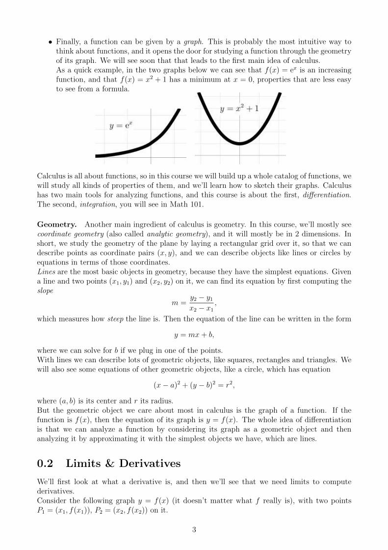
• Finally, a function can be given by a graph. This is probably the most intuitive way tothink about functions, and it opens the door for studying a function through the geometryof its graph. We will see soon that that leads to the first main idea of calculus.As a quick example, in the two graphs below we can see that f(x) = ex is an increasingfunction, and that f(x) = x2 + 1 has a minimum at x = 0, properties that are less easyto see from a formula.

Calculus is all about functions, so in this course we will build up a whole catalog of functions, wewill study all kinds of properties of them, and we’ll learn how to sketch their graphs. Calculushas two main tools for analyzing functions, and this course is about the first, differentiation.The second, integration, you will see in Math 101.

Geometry. Another main ingredient of calculus is geometry. In this course, we’ll mostly seecoordinate geometry (also called analytic geometry), and it will mostly be in 2 dimensions. Inshort, we study the geometry of the plane by laying a rectangular grid over it, so that we candescribe points as coordinate pairs (x, y), and we can describe objects like lines or circles byequations in terms of those coordinates.Lines are the most basic objects in geometry, because they have the simplest equations. Givena line and two points (x1, y1) and (x2, y2) on it, we can find its equation by first computing theslope

m =y2 − y1

x2 − x1

,

which measures how steep the line is. Then the equation of the line can be written in the form

y = mx+ b,

where we can solve for b if we plug in one of the points.With lines we can describe lots of geometric objects, like squares, rectangles and triangles. Wewill also see some equations of other geometric objects, like a circle, which has equation

(x− a)2 + (y − b)2 = r2,

where (a, b) is its center and r its radius.But the geometric object we care about most in calculus is the graph of a function. If thefunction is f(x), then the equation of its graph is y = f(x). The whole idea of differentiationis that we can analyze a function by considering its graph as a geometric object and thenanalyzing it by approximating it with the simplest objects we have, which are lines.

0.2 Limits & Derivatives

We’ll first look at what a derivative is, and then we’ll see that we need limits to computederivatives.Consider the following graph y = f(x) (it doesn’t matter what f really is), with two pointsP1 = (x1, f(x1)), P2 = (x2, f(x2)) on it.

3

For reasons which will become clear later on, we want to approximate the graph at each pointby a line, i.e. we want to find the line that at that point is most ’similar’ to the graph. Theline that does this is the ’tangent line’, which goes through the point in the same direction asthe graph. That direction is the slope of the line. In this picture, let’s say the tangent linethrough P1 has slope m1 = 1

2and the one through P2 has slope m2 = −1. The derivative is a

new function that keeps track of all these slopes.

The derivative of f is the function f ′ that for any x0 gives theslope of the tangent line to the graph y = f(x) at (x0, f(x0)).

Suppose the two lines above have equations y = m1x+ b1 and y = m2x+ b2. Then we have

f ′(x1) = m1, f ′(x2) = m2.

This definition is a bit tricky but it’s crucial. Students often mistakingly say things like ’thederivative is the tangent line’ or ’the derivative is the slope of the tangent’, which are wrongand lead to confusion. A derivative is a function, and its value for a given x is the slope of thetangent line to the graph above that x. And the graph we’re talking about is the graph of theoriginal function f , whose derivative is the function f ′.

As a first example of why this might be useful,consider the picture on the right. This shouldillustrate that at points where the graph has amaximum or minimum, the tangent lines arehorizontal. We’ll see later that this gives aneasy way to detect a maximum or minimum.

In many applications, that’s exactly what we want: the function might give the cost of some-thing, and we would like to minimize that cost.

But this wouldn’t be useful unless we had some (easy) way of computing the derivative of afunction. We do, of course, and that’s what this course is about. First we’ll see how to computethe slope of the tangent line to a graph at some point. To do this we introduce secant lines,which is just a fancy name for a line through two points on a graph.

4

For such a line, the slope is easy to compute, if we know the two points P and Q that determinethe secant line. Let’s name the points P = (xP , f(xP )) and Q = (xQ, f(xQ)). Then the slopeformula y2−y1

x2−x1 we saw above gives us the slope mPQ of the secant line,

mPQ =f(xQ)− f(xP )

xQ − xP.

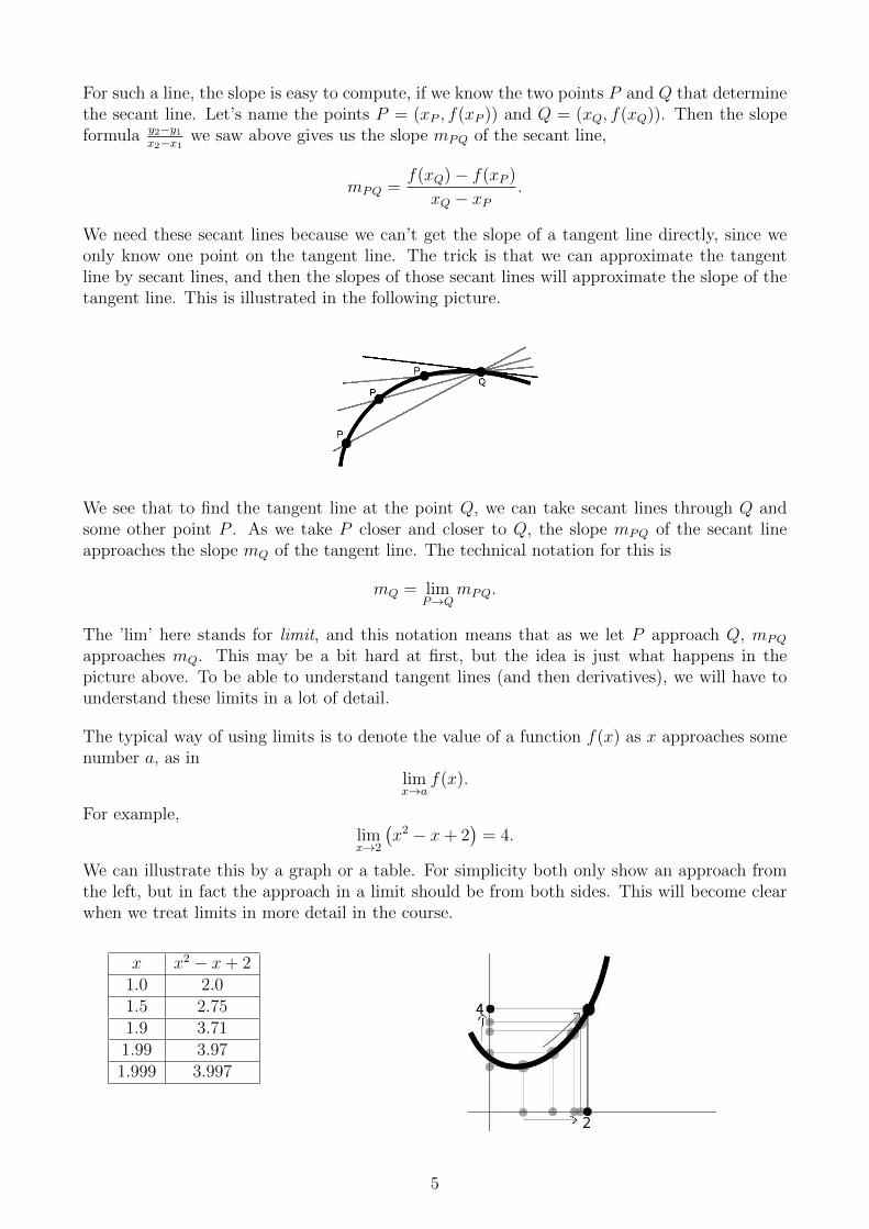
We need these secant lines because we can’t get the slope of a tangent line directly, since weonly know one point on the tangent line. The trick is that we can approximate the tangentline by secant lines, and then the slopes of those secant lines will approximate the slope of thetangent line. This is illustrated in the following picture.

We see that to find the tangent line at the point Q, we can take secant lines through Q andsome other point P . As we take P closer and closer to Q, the slope mPQ of the secant lineapproaches the slope mQ of the tangent line. The technical notation for this is

mQ = limP→Q

mPQ.

The ’lim’ here stands for limit, and this notation means that as we let P approach Q, mPQ

approaches mQ. This may be a bit hard at first, but the idea is just what happens in thepicture above. To be able to understand tangent lines (and then derivatives), we will have tounderstand these limits in a lot of detail.

The typical way of using limits is to denote the value of a function f(x) as x approaches somenumber a, as in

limx→a

f(x).

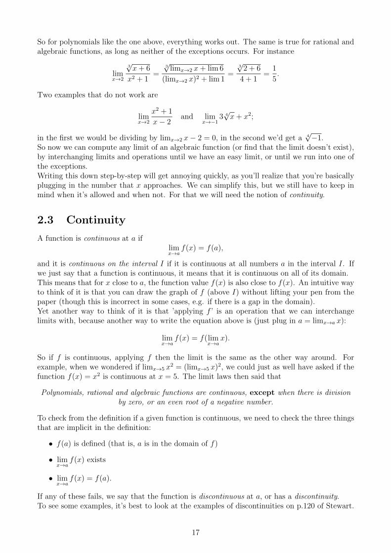
For example,limx→2

(x2 − x+ 2

)= 4.

We can illustrate this by a graph or a table. For simplicity both only show an approach fromthe left, but in fact the approach in a limit should be from both sides. This will become clearwhen we treat limits in more detail in the course.

x x2 − x+ 21.0 2.01.5 2.751.9 3.711.99 3.971.999 3.997

5

Let’s go through a complete example of computing the slope of a tangent line to a graph at apoint. Let the graph be y = x2 +x and the point Q = (xQ, x

2Q+xQ) = (0, 0). Then the equation

of the tangent line looks like y = mQx (because plugging x = 0, y = 0 into y = mQx+ b givesb = 0), and we wish to compute mQ.Let P = (xP , x

2P +xP ) be the point that will approach Q. Then by the formula above the slope

of the secant line is

mPQ =f(xP )− f(xQ)

xP − xQ=

(x2P + xP )− 0

xP − 0

=xP (xP + 1)

xP= xP + 1.

Now we can write down the slope mQ of the tangent line as a limit with P approaching Q.Note that actually we only need to let xP approach xQ = 0. So

mQ = limP→Q

mPQ = limxP→0

(xP + 1) = 1.

That’s all. Now we know that the tangent line at the origin has slope 1, and the equation ofthe tangent line is y = 1 · x = x. Most of what we will do in this course is building up themachinery that we need to do this systematically for much more complicated functions.We can also write down the result above in terms of the derivative f ′ of f(x) = x2 + x,

f ′(0) = 1.

By itself that’s not very useful notation. But we will learn how to compute that

f ′(x) = 2x+ 1

as a function, and then the above computation can be replaced by just plugging in f ′(0) =2 · 0 + 1 = 1. That will save a lot of time.

The main skill we’ll have to learn is computing derivatives of functions, starting with thedefinition

f ′(x) = limy→x

f(y)− f(x)

y − x.

This is just what we did above: inside the limit is the slope of a secant line between two pointson the graph, we take the limit as one point approaches the other, so that the secant linesapproach the tangent line, and we get out of it the slope of the tangent line.

This might still seem pretty complicated, but we’ll learn how to take any function, break it intosimpler pieces, take the derivatives of those pieces, and then put them back together. That waywe will be able to differentiate (a different word for ’computing the derivative of’) just about

6

f(x) ax+ b x2 x3 x3 + x2 + 5x x2 + xf ′(x) a 2x 3x2 3x2 + 2x+ 5 2x+ 1

f(x) 1x

√x sinx cosx ex

f ′(x) −1x2

12√x

cosx − sinx ex

any reasonable function, as long as we know the derivatives of a number of basic functions.The table below displays some of these basic derivatives. You don’t need to understand themyet, but you might already see some sort of pattern.As a simple example of how we can break functions up into smaller pieces, consider f(x) =x3 + x2 + 5x from the first row of the table. It splits up like this:

f ′(x) = (x3 + x2 + 5x)′ = (x3)′ + (x2)′ + (5x)′ = 3x2 + 2x+ 5.

0.3 Applications

Finally, let’s take a quick look at one application of differential calculus, optimization. This isonly one of the many applications we will see in this course, but it’s a good example, becauseit’s easy to see the use of it, as well as why calculus is necessary for it.

By optimization we mean finding the input value for which a certain function returns thebest possible output. ’Best’ means either a maximum or a minimum: if your function tellsyou the money you make from an investment, then you might want to maximize that, or ifthe function gives the distance of the route that you’re taking somewhere, then you want tominimize that. The observation that we made before about a maximum or minimum having ahorizontal tangent line is what allows us to find it using the derivative.Let’s look at a very simple example, the function f(x) = 2x− x2. Here’s what its graph lookslike:

With your future differentiating skills you will easily see that the derivative of f is f ′(x) = 2−2x.So for any number a on the x-axis, we know that f ′(a) = 2− 2a is the slope of the tangent lineto the graph of f at the point (a, f(a)). And to find the maximum we need to find the pointthat has a horizontal tangent line, in other words a point where the slope of the tangent line iszero. So we just have to solve the equation

f ′(a) = 2a− 2 = 0 ⇒ a = 1.

That means that the only place the graph can have a horizontal tangent line is at a = 1, soif it has a maximum or a minimum anywhere, it must be there. Now the value of f there isf(1) = 1, while at for instance x = 0, it is f(0) = 0, so it can’t be a minimum, since f(0) issmaller. Hence f(1) must be a maximum.

7

Indeed, this corresponds to what we see in the picture, the question mark is exactly in between0 and 2. Of course, we could have seen that from the graph right away, but the point is thatif we can do it without looking at the graph, we will also be able to do it for much harderfunctions, whose graphs may be much harder to draw.This is still a pretty abstract application, but here’s a more concrete situation where we coulduse it. Imagine a lifeguard standing on the beach at the water’s edge. He sees a person in thewater screaming for help, 100m further down the beach and 100m into the water. Suppose hecan swim 1m/s and can run 2m/s. Of course he wants to get there as soon as possible, butshould he jump straight in and swim diagonally (that’s

√2 · 100 ≈ 141m), or should he run the

100m along the water first and then swim the 100m? Well, swimming diagonally would take141m1m/s

= 141 seconds, while the other way would take 100m2m/s

+ 100m1m/s

= 150 seconds. So should hejump right in?Well, he can also run along the water some of the way, and swim from there. Suppose he runs20m, then he will have to swim

√802 + 1002 = 128m, and he will get there in 20m

2m/s+ 128m

1m/s= 138

seconds, that’s a bit faster! But can he do any better?We won’t do it now, because it’s a bit too hard, but you can write down a function for thetime, dependent on how far the lifeguard runs along the water. Then if like above you lookfor horizontal tangent lines, you’ll find that it has a maximum somewhere in between, whichcorresponds approximately to running 42m along the water. Doing this will take him 137seconds, and he can be certain that there’s no faster way.Of course, it’s hard to imagine a lifeguard getting his notebook out to save a few seconds, anddoing calculations for probably a few minutes (depending on how well he paid attention in hiscalculus class). But hopefully you see that this way we can solve a problem in an exact way,that we couldn’t really have found an answer for in any other way.

8

Chapter 1

Functions

1.1 Functions • 1.2 Graphs of Functions • 1.3 Catalog of Functions • 1.4 Combining Functions

1.1 Functions

Abstractly, a function is a rule that for each element of one set D gives an element of anotherset E. The set D is called domain of the function, and E is the range. The notation for afunction is

f : D → R.

The way to think of an abstract function is as a group of arrows between two blobs (the sets):each arrow then goes from one element in the domain to one element in the range, and fromeach element, there is only one arrow going to the range, while each element of the range canbe pointed to by zero, one, or more elements from the domain.

In this course, the domains will always be ’intervals’ of ’real numbers’. I’ll have to sidetrackhere to explain what those things mean.

A real number is a number that you can write down in (possibly infinite) decimal notation. This in-cludes whole numbers (also called integers), like 0, 1, 2, 13, -5, it includes rational numbers like 1

3 =0.333 · · · , 57 = 0.714 · · · , −172 = −8.5, and then there are the irrational numbers. Some irrational numbers

have familiar forms like√

2, π, e, but others only exist in decimal notation, like 0.123456789101112 · · · .The collection of all of the real numbers is denoted by R.

9

Another, more intuitive, way to think of R is as ’the real line’: imagine a line, infinite in both directions,with marks for 0 and 1. Then every real number has a place on this line, and every spot on this line is areal number.Mathematicians have more precise definitions of R, but we don’t need those in calculus.An interval is a segment of the real line, or a combination of several (or even infinitely many) segments.Examples of basic intervals are

[1, 2], (5, 7), [0, 2π), (−1, 3].

So an interval is described by its start and end point, and the type of bracket (’[’ or ’(’) tells you whetherthe start/end point is in the interval (if ’[’), or not in it (if ’(’). In general, an interval is a combinationof basic intervals like those above, for instance

[1, 3] ∪ [4, 5) ∪ (5, 6].

Note that 5 is not in this interval.

We will also have to work with infinite intervals like [0,∞), (−∞, 2] and (−∞,∞) = R. But be warned

that this is just notation, ∞ is not a number!

Finally, note that this interval notation is closely related to inequalities: [2, 3) is the set of real numbers

x such that x ≥ 2 and x < 3.

So in this course, the definition of function will be:

A function (with domain D and range E, both intervals) is a rule that for each number in Dgives a number in E.

Functions as FormulasThis abstract definition is good for understanding functions, and setting the boundaries of whatthey can be, but in practice it’s not so useful. No one wants to describe a function by drawinga diagram with infinitely many arrows! So within this universe of abstract functions, we reallyonly deal with the small world of functions that can be concretely described by some kind offormula. Some basic examples are

2x+ 3, x2,√x− 2,

1

x2 + 1, |x|, sinx, ex, ...

We will catalog some of these basic kinds of functions in section 3. And then there are severalways to combine functions to create new ones, see section 4.Functions given by formulas are easier to deal with, because we can manipulate their formulasusing algebra. But we would still be kind of helpless if we didn’t have a more intuitive or visualway to think about functions.

1.2 Graphs of Functions

The graph of a function is the set of points in the xy-plane given by the coordinates (x, f(x)),where x can be any number in the domain of f . We think of a graph as the picture we getwhen we take the domain on the x-axis in the xy-plane, and then straight above each x in thedomain we draw a point at height f(x). But note that a graph can be infinite, and the picturewe draw is only a finite snapshot of it.Another way of describing the graph of f is as the set of points (x, y) that satisfy the equationy = f(x). For instance, the graph of the function f(x) = x2 is a parabola, and is also given bythe equation y = x2. There are other curves that are given by an equation but that are not thegraph of some function. For example, the equation x2 + y2 = 1 gives a circle, which is not thegraph of a function. We know that it’s not the graph of a function because for some x-valuesthere are more than 1 points above (or below) it, for example with x = 0 the circle contains(0, 1) and (0,−1). We can summarize this as the Graph Test, which we can use to check if agiven curve is the graph of some function:

10

A curve is the graph of a function if for each x there is at most 1 point on the curve with thatx-coordinate.

Note that for some x there might be no point on the graph with that x-coordinate; then thatx is not in the domain.

1.3 Catalog of Functions

We will take a quick tour through the zoo of functions, focusing on the formulas and domainsof the most important functions. For more detail (and pictures), see Stewart 1.2.When we talk about the domain of a function, we really mean the biggest domain that thatkind of function can have: if you have a function on a certain domain, you can always restrictthe function to a smaller domain. So when I say ’the domain of a constant function is R’, itmeans that the biggest domain a constant function can have is R, even though it could alsohave a smaller domain.On the last page you can see graphs of some of the basic functions; it’s useful to know these byheart.

• Constant Functions The simplest kind of function just always gives the same value, nomatter what the input:

f(x) = c

for some real number c. These functions are so simple they’re boring, but sometimes itis important to remember that they’re still functions. The domain is R, and the graph isjust a horizontal line.

• Linear Functions A linear function looks like

f(x) = ax+ b

for two real numbers a and b. They’re the next simplest kind, but already much moreinteresting. In fact, calculus is based on using linear functions to analyze any function.The domain is R and the graph is a line, but it cannot be a vertical line: a vertical linecannot be the graph of a function because it has more than one point above one value ofx.

• Polynomials A polynomial is a function that is built up out of addition and multiplica-tion, for instance

x2 + 1 or 2x7 − 3x4 − 5.

Constant and linear functions are of course also polynomials. Polynomials have domainR.

• Rational Functions Rational functions are built up out of addition, multiplication anddivision. Using basic algebra we can always rearrange such a function into a fraction oftwo polynomials, like

x5 + 2

x2 − 2or

x− 1

x2 + 7.

Because we cannot divide by zero, a rational function is not defined at the x for whichits denominator is zero. The first example above is not defined at 2 or −2, so its domainconsists of all real numbers except 2 and −2. On the other hand, the second example is

11

defined for all real numbers, because x2 + 7 is always greater than 7.But sometimes we have to be careful. The rational function

x3 − 1

x2 − 1

looks like it might not be defined at 1, but if we simplify

x3 − 1

x2 − 1=

(x− 1)(x2 + x+ 1)

(x− 1)(x+ 1)=x2 + x+ 1

x+ 1,

we see that x = 1 actually is in the domain. The easy way to check if this might happenis to see if the numerator is zero for the x that you think is not in the domain. Forinstance, for x = 1 the numerator was 13 − 1 = 0, but for x = −1 the numerator is(−1)3 − 1 = 2 6= 0, so −1 is indeed not in the domain.

• Algebraic Functions Algebraic functions are built up out of addition, multiplication,division and roots (

√·, 3√·, 4√·,...). For example,

√x+ 1 and

x2 +√x+ 1√

1− x2.

Domains of algebraic functions are trickier. Aside from avoiding division by zero, we mustalso avoid taking even roots of negative numbers. The ’even roots’ are

√·, 4√·, 6√·,..., and

we cannot take an even root of a negative number, because if for instance√−8 = a, then

a2 = −8, which is not possible because squares are always positive. On the other hand,there is no problem with 3

√−8 = −2, since (−2)3 = −8.

So the domain of the first example above is where x + 1 ≥ 0, i.e. [−1,∞). The domainof the second example is more complicated: because of the

√x, we must have x ≥ 0, and

because of the√x2 − 1 we must have x ≤ 1. But we also cannot have x = 1, because

then we would divide by zero. Hence the domain is [0, 1).

• Trigonometric, Exponential & Logarithmic We will devote more time to these later.Trigonometric functions are sin x, cosx and all their family members, exponential func-tions are of the form ax, and logarithmic functions are of the form loga x, where a > 0 isthe base of the logarithm. The only one of these with an unusual domain is loga x, whichhas domain (0,∞).

• Many More... Just so you don’t think that these are somehow all the functions weknow, I should say that there are many more functions out there. Below you’ll see thatwe can combine any known functions to get new ones, which sometimes have completelynew behavior. Later we’ll also see inverse functions like arcsin = sin−1. At the end ofthe course we’ll see Taylor Series, which open the door for defining lots of new functions,although we won’t really go into that in this course. And there’s many, many more.

1.4 Combining Functions

Simple combinationsThere are several ways to combine functions to build new ones. For instance, we can add,multiply or divide two functions. For instance, let f(x) =

√x+ 1 and g(x) = 2x− 4. Then the

12

new functions f + g, f · g = fg, fg

= f/g are determined by

(f + g)(x) = f(x) + g(x) =√x+ 1 + 2x− 4,

(fg)(x) = f(x) · g(x) =(√

x+ 1)· (2x− 4) ,

f

g(x) =

f(x)

g(x)=

√x+ 1

2x− 4.

Think about the domains of these new functions: a point is only in the domain of the newfunction if it was in the domain of both the old functions. BUT there is one exception for f/g:because dividing by zero is never allowed, the denominator function shouldn’t take the value0. In this example, we don’t want 2x − 4 = 0, which solves to x = 2. So x = 2 is not in thedomain of f/g, even though it is in the domain of f and g.

CompositionThe second most important way of making new functions is composition. The composition oftwo functions f and g is the function f ◦ g, defined by

(f ◦ g)(x) = f(g(x)).

For example, if f(x) =√x and g(x) = x+ 3, then

(f ◦ g)(x) =√g(x) =

√x+ 3.

So f ◦ g is the function that first does g to x, and then does f to the result of that.As you may guess, determining the domain of f ◦ g is a bit trickier: it consists of all x in thedomain of g such that g(x) is in the domain of f . In the example the domain of g is all of R,but the only x from R that are in the domain of f ◦ g are the ones for which g(x) = x+ 3 is inthe domain of f , which is [0,∞). So we need the x for which x+ 3 is in [0,∞), which happensfor x ≥ −3, so the domain of f ◦ g is [−3,∞).

GlueingAnother way to create new functions is take two (or more...) functions, restrict their domainsso that they don’t overlap, and then glue the two functions together.For example, take f(x) = −x and f(x) = x. Restrict the domain of f to (−∞, 0] and that off to (0,∞), so they don’t overlap. Then glueing them gives this the familiar absolute valuefunction |x|. This is called a piecewise defined function, and we describe it with curly bracketnotation:

|x| ={

x if x ≥ 0−x if x < 0.

13

Chapter 2

Limits and Continuity

2.1 Definition • 2.2 Computing Limits • 2.3 Continuity • 2.4 Examples of limits

2.1 Definition

Our main definition is the following.

limx→a

f(x) = L

means that however x approaches the fixed number a, thevalue of the function at x, f(x), approaches the number L.If such an L does not exist, we say that the limit does notexist.

Note that in this definition the value of f at a itself does not matter.For example, the following picture illustrates this for limx→2 (x2 − x+ 2) = 4:

The tricky part of this definition is the different ways that x can approach a. For instance, xcan approach a from the left or the right, and the result for f(x) might be different. Considerthe following graph, which uses the graphing convention that an open circle means that thatpoint is not on the graph; here f(1) = 1, not 2.

14

Here as x goes to 1 from the left, f(x) goes to 1, but if x comes from the right, f(x) goes to2. So in this case, the definition above tells us that limx→1 f(x) does not exist, because twodifferent ways of approach give different approached values. Nevertheless, we would still like tohave notation for one-sided limits, which only involve the x on one side of a.

We write limx→a−

f(x) = L

if as x approaches a from the left, f(x) approaches L.Similarly, we write

limx→a+

f(x) = L

if as x approaches a from the right, f(x) approaches L.

So be warned, a tiny change of notation (a− instead of a) makes a big difference in meaning.In the second graph above, where the two-sided limit did not exist, we have

limx→1−

f(x) = 1 and limx→1+

f(x) = 2.

It is still possible for a one-sided limit to not exist. For example, limx→01x2

does not exist,because as x gets smaller and smaller, 1

x2gets bigger and bigger, so does not approach any

number.This gives a way to check if a two-sided limit exists, by first checking if the two one-sided limitsexist, and then seeing if their values are equal.

We have limx→a

f(x) = L

if bothlimx→a−

f(x) = L and limx→a+

f(x) = L.

If the left and right limit are not equal, or if one of theone-sided limits does not exist, then the (two-sided) limitdoes not exist.

So in the first graph above, we have limx→2 f(x) = 4 since the left and right limits are bothequal to 4. In the second graph, limx→1 f(x) does not exist, since the left and right limits aredifferent.This left/right approach is especially convenient (and necessary) for piecewise defined functions,when the number a is on the border between two of the pieces. The most common example ofthis is the absolute value function, so let’s look at

limx→0|x|.

To determine the existence and value of this limit, we need to look at the one-sided limitsfirst. For the left-hand limit, we only need to consider x with x < 0, for which the definition of|x| says |x| = −x. Hence

limx→0−

|x| = limx→0−

(−x) = 0.

The last step is true because as x approaches 0, so does −x.Similarly,

limx→0+

|x| = limx→0+

x = 0.

So indeed the left and right limit are equal, and we can conclude that limx→0 |x| = 0.Of course the above limit would have been easy to see from the graph of |x|, but we want to beable to determine limits without looking at the graph of the function, especially because later

15

on we will have to use limits to draw graphs.As another example, consider

f(x) =

{2x− 1 if x ≤ 1x2 if x > 1.

Then to the left of x = 1, the function is gives by 2x − 1, and on the right by x2, so if wecalculated the two one-sided limits separately, we get

limx→1−

f(x) = limx→1−

(2x− 1) = 2

(limx→1−

x

)− 1 = 2 · 1− 1 = 1,

limx→1+

f(x) = limx→1+

x2 =

(limx→1+

x

)2

= 12 = 1.

So the left and right limits exist and both equal, hence we can conclude that limx→1 f(x) = 1.

Remark that when we say ’x approaches a’, we don’t care about what happens when x equalsa, since that is not part of the approach. If instead of |x| we considered the (weird) function

h(x) =

−x if x < 013 if x = 0x if x > 0,

the left and right limits would still be 0, so the limit exists and limx→0 h(x) = 0, even thoughh(0) = 13.

2.2 Computing Limits

The following example illustrates the basic approach to computing limits of functions given bynice formulas.

limx→5

(2x2 − 3x+ 4) = limx→5

(2x2) + limx→5

(−3x) + limx→5

4

= 2(limx→5

x)2 − 3(limx→5

x) + (limx→5

4)

= 2 · 52 − 3 · 5 + 4 = 50− 15 + 4 = 39.

The idea is to reduce the big limit to several small limits which are easy to determine, usuallyone of the types

limx→a

x = a or limx→a

b = b.

Since the left/right issue is not a problem for these two easy limits, we do not have to worryabout that in this approach.The question is if all the steps above are actually valid: is it true for instance that

limx→5

x2 =(

limx→5

x)2

?

We call this ’interchanging the order of the operations’: on the left you square x first and thenconsider the limit of that, on the right you first take the limit and then square that.This is what the ’limit laws’ (Stewart 2.3) answer: can we interchange the limit operation withthe basic arithmetic operations? I like to summarize these laws as follows:

Limits interchange perfectly with addition, multiplication, division and root taking, exceptthat we can’t divide by 0, and we can’t take even roots of anything negative.

16

So for polynomials like the one above, everything works out. The same is true for rational andalgebraic functions, as long as neither of the exceptions occurs. For instance

limx→2

3√x+ 6

x2 + 1=

3√

limx→2 x+ lim 6

(limx→2 x)2 + lim 1=

3√

2 + 6

4 + 1=

1

5.

Two examples that do not work are

limx→2

x2 + 1

x− 2and lim

x→−13 4√x+ x2;

in the first we would be dividing by limx→2 x− 2 = 0, in the second we’d get a 4√−1.

So now we can compute any limit of an algebraic function (or find that the limit doesn’t exist),by interchanging limits and operations until we have an easy limit, or until we run into one ofthe exceptions.Writing this down step-by-step will get annoying quickly, as you’ll realize that you’re basicallyplugging in the number that x approaches. We can simplify this, but we still have to keep inmind when it’s allowed and when not. For that we will need the notion of continuity.

2.3 Continuity

A function is continuous at a iflimx→a

f(x) = f(a),

and it is continuous on the interval I if it is continuous at all numbers a in the interval I. Ifwe just say that a function is continuous, it means that it is continuous on all of its domain.This means that for x close to a, the function value f(x) is also close to f(x). An intuitive wayto think of it is that you can draw the graph of f (above I) without lifting your pen from thepaper (though this is incorrect in some cases, e.g. if there is a gap in the domain).Yet another way to think of it is that ’applying f ’ is an operation that we can interchangelimits with, because another way to write the equation above is (just plug in a = limx→a x):

limx→a

f(x) = f(limx→a

x).

So if f is continuous, applying f then the limit is the same as the other way around. Forexample, when we wondered if limx→5 x

2 = (limx→5 x)2, we could just as well have asked if thefunction f(x) = x2 is continuous at x = 5. The limit laws then said that

Polynomials, rational and algebraic functions are continuous, except when there is divisionby zero, or an even root of a negative number.

To check from the definition if a given function is continuous, we need to check the three thingsthat are implicit in the definition:

• f(a) is defined (that is, a is in the domain of f)

• limx→a

f(x) exists

• limx→a

f(x) = f(a).

If any of these fails, we say that the function is discontinuous at a, or has a discontinuity.To see some examples, it’s best to look at the examples of discontinuities on p.120 of Stewart.

17

The game is now to determine which functions are continuous where on their domains, andespecially if the basic functions are continuous on all of their domain.Of course, outside of its domain a function is not defined, so the first of the three conditionsabove fails, and the function is certainly not continuous. By the limit laws, all algebraicfunctions are continuous on their domains; the two exceptions correspond to points outside ofthe domains. For instance, the function 1

xis continuous on its domain, which consists of all

real numbers except for 0. Since the function is not defined at 0, it doesn’t make much senseto say that it’s continuous there or not.The same is true for exponential and trigonometric functions, and their inverses (which we’llmeet later): they are all continuous on all of their domain. But note that some of thesefunctions do not have all of R as their domain; for instance, integer multiples of π/2 are not inthe domain of tanx = sinx/ cosx, since there cosx is 0.So in summary, all the elementary functions above are continuous on their domains. Of thethree conditions, only the first one ever fails for these functions, mostly because of division byzero or even roots of negative numbers. When the second and third condition fail, it is mostoften for piecewise defined functions (including |x|), which is why most continuity questions inthe book or the homework are about such functions.The final thing to know is:

A composition of two continuous functions is continuous as well.

With that fact we can figure out if any function given by some sort of formula is continuousor not, by breaking it up as a composition of simple functions, and using what we know aboutthose. The only hard part may be when piecewise defined functions are involved, in which casewe will have to analyze the left and right limits.For example, the function

f(x) =1

2 + sin x

is continuous on its domain (which is R: we never divide by zero because −1 ≤ sinx ≤ 1),because it is a composition f = g ◦ h of the functions g(x) = 1

2+xand h(x) = sinx, a rational

and a trigonometric function, both of which we know to be continuous.On the other hand, the function

f(x) =

x2 + 1 if x < 11 if x = 12x

if x ≥ 1.

is not continuous at x = 1. We check the three conditions for continuity:

• The function is clearly defined at x = 1.

• To find limx→1 f(x), we need to check the left and right limits (because it’s piecewisedefined):

limx→1−

f(x) = limx→1−

x2 + 1 = 2, limx→1+

f(x) = limx→1+

2

x= 2.

Since the two one-sided limits are equal, the two-sided limit exists, and limx→1 f(x) = 2.

• But limx→1 f(x) = 2 6= f(1)!

So one of the conditions fails, and the function is not continuous at x = 1. At all other x,however, the function is given by x2 + 1 or 2

x, which we know to be continuous, except for 2

xat

x = 0, but that doesn’t happen. So this f(x) is continuous at all x except 1.

18

2.4 Examples of Limits

Right now we have two main methods for computing limits:

• We can interchange limits and continuous functions, until we end up with easy limits, orwe run into one of the exceptions. In practice, we do this by saying why the function iscontinuous (if it is), and then just plugging in.

• We can compute the left and right limits, and see if they are equal. Especially useful forpiecewise defined functions.

In later chapters we will add to this two harder approaches, the Squeeze Theorem and Taylorseries.

Many of the limit questions on exams are however of a slightly different nature: they requiresome algebraic trick before one of the methods above can be applied. We give some examplesof these.The most common kind is the following type of limit calculation:

limx→1

x2 − 1

x− 1= lim

x→1

(x− 1)(x+ 1)

x− 1= lim

x→1x+ 1 = 2.

Here the function is a rational function that seems to be undefined at the number that xapproaches, so we couldn’t just plug in. But after a cancellation there is no problem at all.What makes it hard is that the factors that cancel each other may be hidden, and you wil haveto factor a polynomial first. Another example is

limx→−4

x2 + 5x+ 4

x2 + 3x− 4= lim

x→−4

(x+ 4)(x+ 1)

(x+ 4)(x− 1)= lim

x→−4

x+ 1

x− 1=

3

5.

Another very common kind looks like this:

limx→9

√x− 3

x− 9= lim

x→9

√x− 3

x− 9·√x+ 3√x+ 3

= limx→9

x− 9

(x− 9)(√x+ 3)

= limx→9

1√x+ 3

=1

6.

The trick is that when you see something of the form a+√b in a rational function, multiplying

top and bottom by the conjugate a−√b will lead to (a+

√b)(a−

√b) = a2 − b2, which might

clear up some cancellation.But note that the second kind is actually a lot like the first kind, because for instance we couldhave used x− 9 = (

√x− 3)(

√x+ 3), although such a factorization may be harder to spot.

Another algebraic step that you might have to take is clearing denominators, like in

limx→a

1a− 1

x

x− a= lim

x→a

x−aax

x− a= lim

x→a

x− aax(x− a)

= limx→a

1

ax=

1

a2.

19

Chapter 3

More Limits

3.1 Infinite Limits • 3.2 Limits at Infinity • 3.3 Squeeze Theorem

We will introduce two new kinds of limits:

• Infinite limits are limits that actually don’t exist, but in a specific way, namely as xapproaches a, f(x) keeps growing, for example

limx→0

1

x2=∞, or lim

x→0

−1

x2= −∞.

• Limits at infinity are limits where x keeps getting larger (either positive or negative; theylook like

limx→∞

1

x2= 0, or lim

x→−∞

1

x2= 0.

When limx→a f(x) is infinite, the graph y = f(x) has the vertical asymptote x = a. For instance,limx→0

1x2

=∞ tells us that x = 0 is a vertical asymptote of y = 1x2

.If limx→∞ f(x) exists and equals L, then y = f(x) has the horizontal asymptote y = L. Forexample, limx→∞

1x2

= 0 implies that y = 0 is a horizontal asymptote of y = 1x2

.

3.1 Infinite Limits

Definition: If however x approaches a, f(x) grows larger than any positive number, we write

limx→a

f(x) =∞,

instead of saying that the limit does not exist. If f(x) grows below any negative number, wewrite limx→a f(x) = −∞.We can make the same definitions for left and right limits, but we won’t spell that out here.For example, limx→a− f(x) =∞ means that if x approaches a from the left, f(x) grows largerthan any positive number (and it doesn’t matter what happens to the right of a).

SubtletiesWhat we mean precisely by ’grows larger than any positive number’ is that no matter how largea number N we take, if we take x close enough to a, f(x) will be larger than N . For instance,we have

limx→0+

1

x=∞

because for any N , if we take x = 1N+1

, which is very close to a = 0, then f( 1N+1

) = 11/(N+1)

=

N + 1 > N . For example, if our big number is N = 1000, then f( 11001

) = 1001, so 1x

grows

20

larger than 1000.In the same way, limx→0−

1x

= −∞, because 1x

grows below any large negative number.

Just like with regular limits, a two-sided infinite limit exists if the corresponding one-sidedlimits both exist and are equal (so both ∞ or both −∞). For example, we just saw thatlimx→0−

1x6= limx→0+

1x, so the two-sided limit limx→0

1x

does not exist, but is not ∞ or −∞!On the other hand,

limx→0−

1

x2=

(limx→0−

1

x

)2

=∞ = limx→0+

1

x2,

so limx→01x2

=∞ (but we could still say that it doesn’t exist).So beware of the difference between a limit not existing, and a limit being infinite. All infinitelimits are limits that do not exist, but not all non-existing limits are infinite. Above we see anexample (limx→0

1x) of a two-sided limit that does not exist, but is not infinite either.

It’s also possible to have a one-sided limit that doesn’t exist, but isn’t infinite. Right now theonly example of a function with a non-existing one-sided limit that we have seen is limx→0+

1x,

which is indeed an infinite one-sided limit, but at the end of this chapter we will see an exampleof a function with a non-existing one-sided limit that is not infinite. (It’s normal if you haveto read this paragraph a couple of times...)Whenever one of limx→a− f(x), limx→a+ f(x) or limx→a f(x) is ∞ or −∞, we say that thevertical line x = a is a vertical asymptote of the graph of f(x). See the end of section 2.2 inStewart for lots of pictures of this.

ExamplesWe’ve now seen one way of showing that a limit is infinite, by arguing from the definition, likewe did for limx→0+

1x

above. From that we can handle 1xa

for any a > 0, as follows:

limx→0+

1

xa=

(limx→0+

1

x

)a=∞a =∞,

where∞a is actually not allowed, and we should instead argue that if you have something thatgoes to∞, and then in the process you take a positive power of it, it will still go to infinity. Forx→ 0−, it’s a bit trickier, because you could have trouble with even roots of negative numbers.Fortunately, now that we’ve settled 1

xa, we don’t need to argue from the definition anymore; we

can do most other examples by reducing to one of those. For example, a limit like limx→11

(x−1)2

we can do with the substitution trick: set u = x− 1. Then 1(x−1)2

= 1u2

, and x→ 1 is the sameas u→ 0. Hence

limx→1

1

(x− 1)2= lim

u→0

1

u2=∞.

A more complicated example, now with the substitution u = x− 2 (so x = u+ 2):

limx→2+

x− 3

x2 − 4= lim

x→2+

x− 3

(x− 2)(x+ 2)= lim

u→0+

(u+ 2)− 3

u((u+ 2) + 2)

= limu→0+

u− 1

u(u+ 4)=

(limu→0+

u− 1

u+ 4

)(limu→0+

1

u

)=−1

4· ∞ =∞.

Of course, there’s plenty of ways to make this more complicated. For one, you first need to seethat you might be dealing with an infinite limit; usually you can tell that when you plug in,you get division by zero, but you don’t get 0

0(in which case there would probably be some kind

of cancellation). This works for rational and algebraic functions, but there are other functionsthat have vertical asymptotes. For example, in limx→0

1sin2(x)

we would get division by zero, but

21

it’s not an algebraic function. Still, we can make the substitution u = sin(x), and use the factthat as x→ 0, also sin(x)→ 0 (in other words, limx→0 sin(x) = 0), and we get

limx→0

1

sin2(x)= lim

u→0

1

u2=∞.

Later we’ll also see that limx→0+ ln(x) = −∞, and that one you can’t recognize as division byzero.

3.2 Limits at Infinity

Definition: We saylimx→∞

f(x) = L

if as x gets bigger and bigger, f(x) approaches L.We can make the same definition for lim

x→−∞. Note again that ∞ is not a number, just notation.

The basic examples are limx→∞1x

= 0 and limx→−∞1x

= 0, which say that as x gets bigger andbigger, 1

xgets closer and closer to 0. More generally, for any number a > 0 we have

limx→∞

1

xa= 0,

because as x grows large, xa grows large as well, so 1xa

becomes small.Almost the same thing is true for x → −∞, except that we would have to avoid taking evenroots of negative numbers.If a limit at infinity exists and equals some number L, then we say that the line y = L is ahorizontal asymptote of the graph of the function. See Stewart 2.6 for several examples andpictures.

The same rules for interchanging apply, except that now we do not want to end up withlimx→±∞ x, but with limx→±∞

1x, because for those we can just write 0. For instance,

limx→∞

(2

x2+

1

x

)= 2

(limx→∞

1

x

)2

+

(limx→∞

1

x

)= 02 + 0 = 0.

However, for limits at infinity we cannot use continuity to justify plugging in, since after all ∞is not a number, so plugging it in does not even make sense. All that we can do is interchangeand then evaluate limx→∞

1x

to 0 everywhere it occurs (although you could still think of it as’plugging in ∞’, but you’re not allowed to say that out loud). In practice, you won’t have towrite down the interchanging steps, but you should write down how you get to the 1

x-form.

Actually, it’s enough to get to 1xa

with a > 0 everywhere, since we know those evaluate to 0 aswell.For rational functions, we do this by dividing top and bottom by the highest power of x thatoccurs, like in

limx→∞

2x2 − x+ 3

3x2 + 5= lim

x→∞

1x2

1x2

· 2x2 − x+ 3

3x2 + 5= lim

x→∞

2− 1x

+ 3x2

3 + 5x2

=2−

(limx→∞

1x

)+(limx→∞

3x2

)3 +

(limx→∞

5x2

)=

2− 0 + 0

3 + 0=

2

3.

22

In general, we see that when the top and bottom polynomials have the same degree, we getthe quotient of the leading coefficients. On the other hand, when the degrees are not the same,two kinds of things can happen:

limx→∞

5x+ 2

2x3 − 1= lim

x→∞

5x2

+ 2x3

2− 1x3

=0 + 0

2− 0= 0,

limx→∞

2x3 − 1

5x+ 2

(=

2− 0

0 + 0

)does not exist (=∞).

We also need this trick of dividing by a power of x for some limits of algebraic functions, butit becomes a bit trickier. For example, (recall x5/2 = x2

√x and x−5/2 ·

√f =

√x−5 · f)

limx→∞

x2 +√x+ 2x5 + 2

x2√x+ 3x2

= limx→∞

1x5/2

1x5/2

· x2 +√x+ 2x5 + 2

x2√x+ 3x2

= limx→∞

1√x

+√

1x5

(x+ 2x5 + 2)

1 + 3√x

= limx→∞

0 +√

1x4

+ 2 + 2x5

1 + 0=√

0 + 2 + 0 =√

2.

As before, we may also have to rationalize or do some other algebra, before we can do theinterchanging.Another kind of example is

limx→∞

(√x2 + 1− x

).

The way to think of it is that as x becomes very large, the +1 becomes insignificant, and wesort of approach

√x2 − x, which should be zero. Working this out formally requires the good

old conjugate trick:

limx→∞

(√x2 + 1− x

)·

(√x2 + 1 + x√x2 + 1 + x

)= lim

x→∞

√x2 + 1

2 − x2

√x2 + 1 + x

= limx→∞

1√x2 + 1 + x

·1x1x

= limx→∞

1x√

1 + 1x2

+ 1=

0√1 + 0 + 1

= 0.

3.3 A nasty example and the Squeeze Theorem

We will give an example of a function whose limit at 0 does not exist, and whose left and rightlimit at 0 do not exist and are not infinite one-sided limits either. Then we will see an exampleof a limit that does exist but for which we need a new method, the Squeeze Theorem.First let’s take another look at the graph of the function sin x:

What is limx→∞ sinx? It depends on how x approaches ∞: if for instance we let x go to ∞over the peaks, where the value is always 1, the limit would be 1. But if x goes over the valleys,where the value is always −1, the limit would be −1. So different approaches of x give differentvalues for the limit, hence the limit does not exist, and is not ∞ or −∞ either. But becausethis is a limit at infinity, there is no left/right distinction.

23

Now consider sin(

1x

), whose graph to the right of zero looks like

What is limx→0+ sin(

1x

)? In the same way as for sinx, different approaches of x give different

limits, so this right limit does not exist, and it is not an infinite limit, either.Let’s go one step further and consider x · sin

(1x

):

It seems that limx→0

(x · sin

(1x

))= 0, but how do we prove that? Interchanging does not work:

since limx→0 sin(

1x

)does not exist, we can’t write lim

(x sin

(1x

))= (limx) · (lim sin

(1x

)). We

also cannot simplify it algebraically.Right now we need to introduce the third method for determining limits, which will help ushandle x sin(1/x):

Squeeze Theorem: Suppose we have g(x) ≤ f(x) ≤ h(x)in some interval around a, and

limx→a

g(x) = L, limx→a

h(x) = L.

Then we can conclude that

limx→a

f(x) = L.

Note that this is not so much a method for calculating a limit, as it is a method of proving thata certain limit really is what we suspect it is.

• For f(x) = x sin( 1x) we can apply the theorem with g(x) = −|x| and h(x) = |x|. Then since

−|x| ≤ x ≤ |x| and −1 ≤ sin(

1x

)≤ 1 we have

−|x| ≤ x · sin(

1

x

)≤ |x|

on all of R, so the condition of the theorem is satisfied, with L = 0 = limx→0−|x| = limx→0 |x|.Hence we conclude that limx→0

(x · sin

(1x

))= 0.

• Another example is

limx→1

√x2 − 1 cos

(2

x− 1

).

We can take g(x) =√x2 − 1 and h(x) = −

√x2 − 1, then we have g(x) ≤ f(x) ≤ h(x) since

−1 ≤ cos(

2x−1

)≤ 1. Since limx→1 g(x) = limx→1 h(x) = 0, we get that

limx→1

√x2 − 1 cos

(2

x− 1

)= 0.

24

In all honesty, in this course we won’t see other applications of the Squeeze Theorem thanfunctions involving sin( 1

x), cos( 1

x) or some variation like cos

(2

x−1

). What’s most important is

to get a sense of such functions, because they provide our only examples of certain possibilities.For instance, limx→0+ sin(1/x) is a one-sided limit that doesn’t exist but doesn’t equal ∞ or−∞. Or x2 sin(1/x) is a differentiable function whose derivative is not continuous; I haven’tshown that but you can check for yourself.

25

Chapter 4

Tangent Lines

4.1 Tangent Lines • 4.2 The Derivative • 4.3 Differentiability • 4.4 Rates • 4.5 Tangent Problems

4.1 Tangent Lines

Definition. The tangent line to a graph y = f(x) at the point (a, f(a)) is the line throughthat point with slope

m = limx→a

f(x)− f(a)

x− a,

if that limit exists.

Recall from the Introduction where this formula came from. Inside the limit is the slope of thesecant line through (x, f(x)) and (a, f(a)), and as x → a, the points come closer and closer,and the slope of the secant line approaches the slope of the tangent line.

Example.To find the equation of the tangent line to y =

√x+ 1 at (3, 2), we compute its slope

m = limx→3

√x+ 1−

√3 + 1

x− 3= lim

x→3

√x+ 1− 2

x− 3·√x+ 1 + 2√x+ 1 + 2

= limx→3

(x+ 1)− 22

(x− 3)(√x+ 1 + 2)

= limx→3

1√x+ 1 + 2

=1√

3 + 1 + 2=

1

4.

So the tangent line has equation y = 14x + b, and plugging in (3, 2) and solving for b gives

2 = 14(3) + b⇒ b = 2− 3

4= 5

4. Hence the equation of the tangent line is y = 1

4x+ 5

4.

Example.Now for y = x3 + 8, at the point (−2, 0). We’ll have to use polynomial division to factorx3 + 8 = (x+ 2)(x2 − 2x+ 4). Then

m = limx→−2

(x3 + 8)− ((−2)3 + 8)

x− (−2)= lim

x→−2

x3 + 8

x+ 2

= limx→−2

(x+ 2)(x2 − 2x+ 4)

x+ 2= lim

x→−2(x2 − 2x+ 4) = 12.

So the tangent line has equation y = 12x + b, and plugging in (−2, 0) and solving for b gives0 = 12(−2) + b = b− 24⇒ b = 24. Hence the equation of the tangent line is y = 12x+ 24.

26

Example.Let’s find the tangent line at a general point (a, a2 + 1) on the graph of f(x) = x2 + 1. Theslope is

ma = limx→a

f(x)− f(a)

x− a= lim

x→a

(x2 + 1)− (a2 + 1)

x− a= lim

x→a

x2 − a2

x− a

= limx→a

(x− a)(x+ a)

x− a= lim

x→a(x+ a) = 2a.

So now we know that for any point on the graph, the slope of the tangent line is 2a. Then wecan also find the equation by plugging (a, a2 + 1) into y = 2ax+ b and solving for b:

a2 + 1 = 2a · a+ b⇒ b = a2 + 1− 2a2 = 1− a2.

Therefore the equation of the tangent line is y = 2ax+ (1− a2).

4.2 The Derivative

In the last example above, we saw that it might not be too hard to give a formula (2a) for theslope of the tangent line at all points a of the graph at once. We can consider that formula asa function (2x), which is the main object of study in differential calculus.

Definition. The derivative of a function f is the function f ′ that gives theslope f ′(a) of the tangent line to the graph y = f(x) at a point (a, f(a)), foreach a in the domain of f at which the tangent line exists.

More precisely, the derivative is given by the limit that defines the slope of the tangent line (ifit exists):

f ′(a) = limx→a

f(x)− f(a)

x− a= lim

h→0

f(a+ h)− f(a)

h.

The second formula is new, so let us check that they are the same. In the first, we let x approacha, in the second h approaches 0, which means a+ h approaches a. So we replaced x by a+ h,x − a by (a + h) − a = h, and x → a by a + h → h, which is the same as a → 0. There areseveral different notations for the derivative, see p.157 of Stewart. The only one that I oftenuse is

dy

dx=

d

dxf(x) = f ′(x), if y = f(x).

There are (sometimes) two advantages to this notation: you do not need to name the function,which is convenient when you’re talking about a graph y = x2+1 without defining f(x) = x2+1;and it emphasizes the variable x with respect to which you’re taking the derivative, which isuseful when there are parameters (a, b, ...) floating around, or if the variable has an unusualname (like in dy

dt).

See Stewart p.161 for several more notations, including for higher derivatives like

f ′′(x) =d

dx

(d

dxf(x)

)=d2y

dx2.

Finally, instead of saying take the derivative, we use the word differentiate.

In the third example above we saw that for the function f(x) = x2, the slope of the tangentline at (a, a2) is 2a, which we can now rephrase as

f ′(x) = 2x, ord

dxx2 = 2x.

27

What makes this notation so useful is that there is a kind of calculation procedure (which iswhere the word calculus comes from), with which we can differentiate most functions usingstraightforward rules, without having to compute all those limits. Next week we will learn howto do this.For now let’s see two more examples of determining derivatives from the limit definition. Takethe functions f(x) = 1

xand g(x) = 1 +

√x. Then we work out the limits much like in the

examples above:

f ′(a) = limx→a

1x− 1

a

x− a= lim

x→a

a−xxa

x− a= lim

x→a

1

xa

a− xx− a

= limx→a

−1

xa=−1

a2,

g′(a) = limx→a

(1 +√x)− (1 +

√a)

x− a= lim

x→a

√x−√a

x− a·√x+√a√

x+√a

= limx→a

x− a(x− a)(

√x+√a)

= limx→a

1√x+√a

=1

2√a.

To understand derivatives better, it is useful to consider what the graph of the derivative f ′

looks like, given the graph of the original function f . I will not draw pictures, but summarizewhich properties of the graph of f translate into which properties of the graph of f ′. All ofthese can be justified from the interpretation of the derivative as the slope of the tangent line,the last few are clarified in the next section.

• If f is at a maximum or minimum (peak or valley), then f ′ = 0 (intersects the x-axis).

• If f is increasing (going up), then f ′ is positive (above the x-axis).

• If f is decreasing, then f ′ is negative.

• The steeper f (up or down), the larger f ′ (positive or negative).

• If f has a discontinuity, then f ′ does not exist.

• If f has a corner, then f ′ does not exist and has a jump discontinuity there.

• If f has a vertical tangent line, then f ′ has a vertical asymptote.

4.3 Differentiability

Above we defined the tangent line by a limit, but only if that limit exists. It can of coursehappen that that limit does not exist, and we introduce the following word for that.

Definition. We say that a function f is differentiable at a if the tangent line at a exists, i.e. ifthe limit defining the slope of the tangent line exists. We say it is differentiable on an intervalI if it is differentiable at all numbers a in I.

There are 3 basic examples of functions that are not differentiable at some point.• A corner: the typical example of non-differentiability is the function f(x) = |x| at x = 0,for which the slope of the tangent line would be given by

limx→0

|x| − |0|x− 0

= limx→0

|x|x,

which does not exist because the left and right limit are different (−1 and 1). In the graph of|x|, this is easy to recognize: at x = 0 there is a ’corner’ where there couldn’t be a tangent line.

28

• A vertical asymptote: another example is g(x) = 3√x = x

13 at x = 0. Here the slope of

the tangent line would be

limx→0

x13 − 0

x− 0= lim

x→0

1

x23

=

(limx→0

1

x

) 23

=∞,

which means the limit does not exist, hence neither does the tangent line. Again we can see inthe graph what this means: if there was a tangent line, it would have to be vertical. With ourcurrent definition, we do not allow vertical tangent lines, because we do not want to have todeal with the slope being infinite.• A discontinuity: the last kind of example is any function with a discontinuity. Take forexample the function

h(x) =

{x if x < 1

x+ 1 if x ≥ 1,

which has a jump discontinuity at x = 1. Now if we try to compute the left limit (so we useh(x) = x, but h(1) = 2) of the slope of the tangent line at x = 1, we get

limx→1−

h(x)− h(1)

x− 1= lim

x→1−

x− 2

x− 1= −∞.

What happens is that as x approaches 1 from the left, the secant line doesn’t approach atangent line at all, it approaches a vertical line which is clearly not a tangent line. But notethat the limit from the right does exist, and equals 1.

The last example leads to a more general point. For the secant/tangent picture to work at all,the function has to be continuous. We can state and prove this formally: (this is somethingmathematicians like to do a lot, and although in this course we try to spare you, you shouldstill see some examples)

Fact: If f is differentiable at a, then f is continuous at a.Proof: If f is differentiable at a, then limx→a

f(x)−f(a)x−a exists. But as x→ a, the denominator

x−a goes to zero. Then the numerator f(x)−f(a) must go to zero as well, otherwise the limitwould be infinite. So as x→ a we have f(x)− f(a)→ 0, which is equivalent to f(x)→ f(a).This exactly means f is continuous at a.

Turning this statement around, when f is not continuous at a, then it also is not differentiableat a. But it is not true that if a function is continuous, it must also be differentiable: |x| forinstance is continuous, but not differentiable.

4.4 Rates of Change and Velocities

There are different ways of looking at the slope of the tangent line, which I will quickly introducehere. For many more examples, see Stewart 2.7 and the suggested exercises.Think of f(x) as some quantity for which we care about how it changes as a function of x.There are two different ways of measuring the rate of change: we could measure the averagerate of change on some interval [x1, x2]:

f(x2)− f(x1)

x2 − x1

,

or we could measure the instantaneous rate of change at some x1:

limx→x1

f(x)− f(x1)

x− x1

.

29

For instance, p(t) could be the position function of a car, a running athlete, or a moving particle,

as a function of time. Then the average velocity between t2 and t1 is given by p(t2)−p(t1)t2−t1 , the

distance travelled divided by the time spent. On the other hand, the velocity (which is thesame as instantaneous velocity) at time t1 is given by

v(t1) = limt→t1

p(t)− p(t1)

t− t1.

4.5 Tangent Line Problems

There is a large variety of trickier problems involving tangent lines, and usually one of theseshows up on the exam. I will give examples of the most typical ones here, although I’ll onlywork out one of them, since they will become easier once we can use the differentiation rules.

• Find the line through (1, 0) that is tangent to y = 1x.

• Find the line through (0, 0) that is normal to y = 1x.

• Find the line that is tangent to both y = x2 and y = x2 − 2x+ 2.

• Find the line that is tangent to y = x4 − 2x2 − x in two different points.

Note that a graph has lots of tangent lines, one for each point. But in these questions, we areasked for a tangent line satisfying some extra condition, like going though some other point noton the graph.I’ll do the first one. Let the line be given by

y = mx+ b.

Then since it goes through the point (1, 0), we get 0 = m · 1 + b, so b = −m and we can assumethe equation is

y = mx−m.

Now we know the line is tangent to y = 1x

at some point, but we don’t know which one yet, solet’s name it (a, 1

a) for now. Above we computed the derivative f ′(x) = −1

x2, and that gives us

the slope of the tangent line at the point (a, 1a), namely m = −1

a2. Hence the equation of our

line looks like

y =−1

a2x+

1

a2.

Finally, the line has to actually go through the point (a, 1a), so we have to have 1

a= −1

a2a + 1

a2.

Multiplying by a2 gives a = −a+ 1, so a = 12. Hence the tangent line we’re looking for is

y = −4x+ 4.

So we have to determine the line by using all the information we’re given step-by-step. In thiscase, it has to pass through (1, 0), meet the graph in some undetermined point (a, f(a)), andit has to be tangent to the graph at that point, so have slope f ′(a).The other questions are similar, but a bit more complicated. For the second, we have to knowwhat normal means: given a line with slope m, the line normal to it is the line with slope −1

m.

And the line normal to a graph (at a certain point) is the line that is normal to the tangent lineto the graph (at that point). So the normal line to the graph y = f(x) at the point (a, f(a))has slope −1

f ′(a), and the equation of the normal line can then be found just like for the tangent

line.The last two questions are quite a bit harder, since they involve two undetermined points,which we’ll both have to name.

30

Chapter 5

Differentiation

5.1 Polynomials • 5.2 Product Rule • 5.3 Quotient Rule • 5.4 Chain Rule

We will introduce the differentiation rules, which will help us compute the derivative of justabout any function, without having to do the limit calculations. However, to justify theserules, and to understand them, we will have to show the limit calculations that are behindthem, which we do in the proofs. You won’t have to be able to reproduce these proofs, or muchless come up with them yourselves. But you can still learn a lot from trying to understandthem.Note that these rules are only valid at values of x where the functions involved are differentiable,but we will not mention that every time.

5.1 Polynomials

We start with the mother of all differential rules:

Power Rule: (xn)′ = nxn−1for any real number n

We could also write this as ddx

(xn) = nxn−1, or f(x) = xn ⇒ f ′(x) = nxn−1. Here are a fewexamples:

(x3)′ = 3x2, , (x17)′ = 17x16, (√x)′ = (x

12 )′ =

1

2x

12−1 =

1

2√x,(

1

x

)′= (x−1)′ = (−1) · x−1−1 =

−1

x2,

(1

x3/2

)′= −3

2· 1

x5/2, (xπ)′ = πxπ−1.

Proving this rule, for any real number, is not so easy (we’ll do it in Ch. 8), but here we willdo it for n a positive integer. We already saw this for x2, and this is what it looks like forf(x) = x3:

f ′(a) = limx→a

x3 − a3

x− a= lim

x→a

(x− a)(x2 + ax+ a2)

x− a= lim

x→a(x2 + ax+ a2) = 3a2.

Here we used the factorization (x3 − a3) = (x − a)(x2 + ax + a2), which may not be easy tocome up with, but is easy to check:

= x(x2 + ax+ a2)− a(x2 + ax+ a2) = (x3 + ax2 + a2x)− (ax2 + a2x+ a3) = x3 − a3.

31

For general n, we can factor xn − an in the same way:

(xn − an) = (x− a)(xn−1 + axn−2 + a2xn−2 + · · ·+ an−3x2 + an−2x+ an−1).

Proof of the power rule: (for n a positive integer) Let f(x) = xn. By definition,

f ′(a) = limx→a

xn − an

x− a= lim

x→a

(x− a)(xn−1 + axn−2 + · · ·+ an−2x+ an−1)

x− a= lim

x→a(xn−1 + axn−2 + · · ·+ an−2x+ an−1)

= an−1 + aan−2 + · · · an−2a+ an−1

= nan−1.

To be able to differentiate any polynomial, and more, we need the following three rules, wherec is a real number:

Constant Rule:ddx(c) = 0

Constant Multiple Rule: (cf )′ = cf ′

Sum Rule: (f + g)′ = f ′ + g′

Note that in the first rule it is better to use the ddx

notation, to make clear that we aredifferentiating with respect to x.Of course the Sum Rule, together with the Constant Multiple Rule, implies a similar rule forsubtractions: (f − g)′ = (f + (−g))′ = f ′ + (−g)′ = f ′ − g′.

Proofs: For the Constant Rule, let f(x) = c. Then

f ′(a) = limx→a

c− cx− a

= limx→a

0 = 0.

Note that the limit is not 00, because c− c is always 0, while x− a is just approaching 0.

The Constant Multiple rule is pretty easy:

(cf)′(a) = limx→a

cf(x)− cf(a)

x− a= lim

x→acf(a)− f(a)

x− a= cf ′(a).

Finally, the Sum Rule is a consequence of the fact that we can interchange limits and sums:

(f + g)′(a) = limx→a

(f(x) + g(x))− (f(a) + g(a))

x− a= lim

x→a

(f(x)− f(a)) + (g(x)− g(a))

x− a

= limx→a

((f(x)− f(a))

x− a+

(g(x)− g(a))

x− a

)=

(limx→a

(f(x)− f(a))

x− a

)+

(limx→a

(g(x)− g(a))

x− a

)= f ′(a) + g′(a).

32

With these rules we can differentiate any polynomial:

(x3 − 2x+ 5)′ = (x3)′ + (2x)′ + (5)′ (sum rule)

= 3x2 + 2(x)′ + 0 (power, constant multiple, constant rule)

= 3x2 + 2, (power rule)

(5x7 + 3x6 − x2)′ = 5(x7)′ + 3(x6)′ − (x2)′ (sum, constant multiple)

= 35x6 + 18x5 − 2x (power rule)

In fact, we can already do more than polynomials:

(3√x+

5

x2+ 7)′ = 3 · 1

2√x

+ 5 · −2

x3+ 0 =

3

2√x− 10

x3.

5.2 The Product Rule

Let’s see what happens when we differentiate the product of two functions. When we saw thesum rule, it said that we could interchange sums with differentiation, just like with limits. Forproducts, that is not at all true: (fg)′ 6= f ′g′! Instead, we have:

Product Rule: (fg)′ = f ′g + fg′

To see why the derivative of products takes this surprising form, we will go through the proof,which is a step harder than the previous ones:

Proof: The trick is to add 0 = (f(a)g(x)− f(a)g(x)) in the middle of the numerator; againthis is not easy to come up with, but we see that it works.

(fg)′(a) = limx→a

f(x)g(x)− f(a)g(a)

x− a= lim

x→a

f(x)g(x) + (f(a)g(x)− f(a)g(x))− f(a)g(a)

x− a

= limx→a

(f(x)g(x)− f(a)g(x)) + (f(a)g(x)− f(a)g(a))

x− a

=

(limx→a

f(x)g(x)− f(a)g(x)

x− a

)+

(limx→a

f(a)g(x)− f(a)g(a)

x− a

)=

(limx→a

g(x) · f(x)− f(a)

x− a

)+

(limx→a

f(a) · g(x)− g(a)

x− a

)=

((limx→a

g(x))·(

limx→a

f(x)− f(a)

x− a

))+

((limx→a

f(a))·(

limx→a

f(a) · g(x)− g(a)

x− a

))= g(a)f ′(a) + f(a)g′(a).

Note that in the second to last step we used the fact that we can interchange limits andproducts, and in the last step we used the continuity of g to get limx→a g(x) = g(a). Weknow that g is continuous because we’re assuming it to be differentiable (see section 4.2).

Now we can use the product rule to compute for instance((x2 − 2) · (x3 − 2)

)′= (x2 − 2)′ · (x3 − 2) + (x2 − 2) · (x3 − 2)′

= 2x · (x3 − 2) + (x2 − 2) · 3x2

= 2x4 − 4x+ 3x4 − 6x2 = 5x4 − 6x2 − 4x.

33

We can actually check this, by first multiplying out and then differentiating the polynomial:((x2 − 2) · (x3 − 2)

)′=(x5 − 2x3 − 2x2 + 4

)′= 5x4 − 6x2 − 4x.

In this case, the second way was actually easier, but later on we’ll see examples where we can’tdo without the product rule.

5.3 The Quotient Rule

Now let’s turn to division. As a starter, let’s differentiate f(x) = 1x

without using the powerrule:

f ′(a) = limx→a

1x− 1

a

x− a= lim

x→a

a−xxa

x− a= lim

x→a

1

xa

−(x− a)

x− a)= lim

x→a

−1

xa=−1

a2,

which is the same as we deduced from the power rule before. In a similar way, we can get ournext rule:

Reciprocal Rule:

(1f

)′= − f ′

f2

So this says that ddx

1f(x) = − f ′(x)

f(x)2 . Let’s see the proof.

Proof: (1

f

)′(a) = lim

x→a

1f(x)− 1

f(a)

x− a= lim

x→a

f(a)−f(x)f(x)f(a)

x− a

= limx→a

1

f(x)f(a)

−(f(x)− f(a))

x− a

=

(limx→a

1

f(x)f(a)

)·(− lim

x→a

(f(x)− f(a))

x− a

)=

1

f(a)2· (−f ′(a)).

Here’s an example, with f(x) = xn:(1

xn

)′= − (xn)′

(xn)2= −nx

n−1

x2n= − n

xn+1,

which we can check by using the Power Rule(1

xn

)′= (x−n)′ = −nx−n−1 = − n

xn+1.

In this case the power rule turned out to be easier, but in the next example it would be helpless:(1

x2 + 1

)′= − (x2 + 1)′

(x2 + 1)2= − 2x

(x2 + 1)2.

34

Now we can do any rational function f(x)g(x)

, by writing it as f(x) · 1g(x)

and applying the productrule and the reciprocal rule. For instance:(

x3 + 1

x2 + 2

)′=

((x3 + 1) · 1

x2 + 2

)′= (x3 + 1)′ · 1

x2 + 2+ (x3 + 1) ·

(1

x2 + 2

)′=

3x2

x2 + 2+ (x3 + 1) ·

(− 2x

(x2 + 2)2

)=

3x2(x2 + 2)

(x2 + 2)2−(

2x(x3 + 1)

(x2 + 2)2

)=

3x4 + 6x2 − 2x4 − 2x

(x2 + 2)2

=x4 + 6x2 − 2x

(x2 + 2)2.

Doing this in general we get the next rule, whose proof we won’t write out here:

Quotient Rule:

(fg

)′= f ′g−fg′

g2

Let’s do the example above again, but now straight from the Quotient Rule:(x3 + 1

x2 + 2

)′=

(x3 + 1)′ · (x2 + 2)− (x3 + 1) · (x2 + 2)′

(x2 + 2)2

=3x2 · (x2 + 2)− (x3 + 1) · 2x

(x2 + 2)2

=x4 + 6x2 − 2x

(x2 + 2)2.

It’s also good to see that the Reciprocal Rule is just a special case of the Quotient Rule:(1

g(x)

)′=

1′ · g(x)− 1 · g′(x)

g(x)2=

0 · g(x)− g′(x)

g(x)2=−g′(x)

g(x)2.

5.4 The Chain Rule

So we know how to do rational functions and roots (since they’re powers), does that mean thatwe can do all algebraic functions? No, because of functions like

F (x) =√x2 + 1,

√x2 +

√x.

They are compositions of functions (F = f ◦ g, f =√x, g(x) = x2 + 1), and even though

we know the derivatives of those (f ′ = 12√x, g′ = 2x), we don’t know the derivative of the

composition (warning: it is not the composition of the derivatives). The solution is the nextrule, which is a bit more complicated than the others, and whose proof we will not do:

35

Chain Rule: If F (x) = f(g(x)), then F ′(x) = f ′(g(x)) · g′(x)

The function F (x) =√x2 + 1 we can write as a composition f◦g with f(x) =

√x, g(x) = x2+1,

whose derivatives are f ′(x) = 12√x

and g′(x) = 2x, so that applying the Chain Rule gives:(√x2 + 1

)′= f ′(g(x)) · g′(x) =

1

2√g(x)

· 2x =x√x2 + 1

.

For F (x) =√x2 +

√x we have F = f ◦ g with f(x) =

√x, g(x) = x2 +

√x, so f ′(x) = 1

2√x

and g′(x) = 2x+ 12√x. Then

F ′(x) =1

2√g(x)

· g′(x) =1

2√x2 +

√x· (2x+

1

2√x

) =(2x+ 1

2√x)

2√x2 +

√x.

We can also prove the Reciprocal Rule using the Chain Rule and the Power Rule. Let F (x) =1

g(x)= f(g(x)), with f(x) = 1

x, f ′(x) = −1

x2. Then(

1

g(x)

)′= F ′(x) = f ′(g(x)) · g′(x) = − 1

g(x)2· g′(x) =

−g′(x)

g(x)2,

just as we derived before from the limit definition.

In the dydx

notation, the Chain Rule is especially easy to remember. Let y = F (x) = f(g(x)),

and write y = f(u), u = g(x). Then f ′(u) = dydu

and g′(x) = dudx

, so we could write the ChainRule as

dy

dx=dy

du· dudx.

In fact this looks a little bit like a proof: just cancel the du’s. But this is not possible, becausethe du’s are not separate objects and these are not really fractions, that’s just notation, as youcan see when you look at it in terms of f and g.

36

Chapter 6

Trigonometric Functions

6.1 Definitions • 6.2 Identities • 6.3 Continuity and limits • 6.4 Derivatives

6.1 Definitions

From high school, you probably know the functions sin(t) and cos(t) as defined by

cos(t) =adj

hyp, sin(t) =

opp

hyp,

where adj, hyp and opp are the lengths of the adjacent, hypotenuse and opposite sides of aright-angled triangle with one angle named t:

Here we do things a bit differently. First of all, the input of the functions sin(t) and cos(t) willalways be in radians, although we may still describe angles in degrees. Recall that to changebetween radians and degrees, all you need to know is

π radians = 180◦.

For instance, a right angle is 90◦ = 12· 180◦ = π

2radians.

Next, in the triangle above the angle t has to be less than π2, otherwise the hypotenuse wouldn’t

intersect the opposite side anymore. But there is a natural way of defining the trigonometricfunctions that allows the t to be any number. Consider a point Pt on a circle with radius 1,such that the line through P and the origin makes an angle t with the x-axis.

37

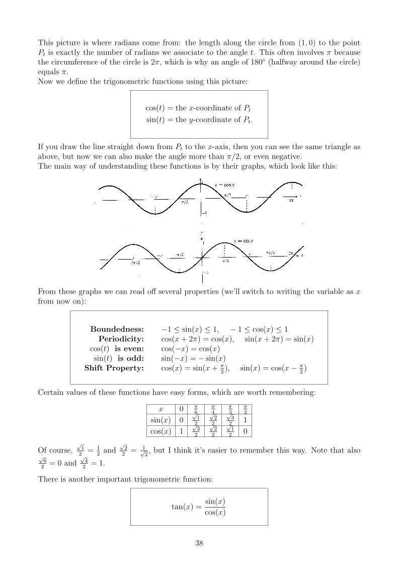
This picture is where radians come from: the length along the circle from (1, 0) to the pointPt is exactly the number of radians we associate to the angle t. This often involves π becausethe circumference of the circle is 2π, which is why an angle of 180◦ (halfway around the circle)equals π.Now we define the trigonometric functions using this picture:

cos(t) = the x-coordinate of Pt

sin(t) = the y-coordinate of Pt.

If you draw the line straight down from Pt to the x-axis, then you can see the same triangle asabove, but now we can also make the angle more than π/2, or even negative.The main way of understanding these functions is by their graphs, which look like this:

From these graphs we can read off several properties (we’ll switch to writing the variable as xfrom now on):

Boundedness: −1 ≤ sin(x) ≤ 1, − 1 ≤ cos(x) ≤ 1Periodicity: cos(x+ 2π) = cos(x), sin(x+ 2π) = sin(x)

cos(t) is even: cos(−x) = cos(x)sin(t) is odd: sin(−x) = − sin(x)

Shift Property: cos(x) = sin(x+ π2), sin(x) = cos(x− π

2)

Certain values of these functions have easy forms, which are worth remembering:

x 0 π6

π4

π3

π2

sin(x) 0√

12

√2

2

√3

21

cos(x) 1√

32

√2

2

√1

20

Of course,√

12

= 12

and√

22

= 1√2, but I think it’s easier to remember this way. Note that also

√0

2= 0 and

√4

2= 1.

There is another important trigonometric function:

tan(x) =sin(x)

cos(x)

38

This function is convenient because it equals oppadj

, which means it relates the angle t with theslope of the hypotenuse. To see this, suppose we have any line y = mx + b. It intersectsthe x-axis in A = (− b

m, 0), and the y axis in B = (0, b). Then A, B and O = (0, 0) form a

right-angled triangle, so if we let t be the angle between the line and the x-axis, we get (with|BO| = b the length of the line segment between B and O, and |AO| = b/m)

tan(t) =opp

adj=|BO||AO|

=b

b/m= m,

or in other words,slope of a line = tan (angle with x-axis) .

Finally there are three other trigonometric functions, which are just reciprocals of the threeabove. Personally, I think they are useless, but they might occur on the final exam. Just try toremember which functions they are reciprocals of, and when you encounter one in a question,rewrite them in terms of cos(x), sin(x) and tan(x), and never look back.

sec(x) =1

cos(x), csc(x) =

1

sin(x), cot(x) =

1

tan(x).

The first one is the secant function, the second the cosecant, and the third is the cotangent.

6.2 Identities

Because of their symmetric definition using the circle, the trigonometric functions satisfy nu-merous identities. We introduce the most important ones.The most basic trigonometric identity is

sin2(x) + cos2(x) = 1,

which is nothing but the Pythagorean Theorem for the triangle with sides sin(t), cos(t) andhypotenuse 1 (the radius of the circle defining the functions).The most important identities are probably the addition formulas:

sin(x+ y) = sin(x) cos(y) + cos(x) sin(y)

cos(x+ y) = cos(x) cos(y)− sin(x) sin(y)

Proving these requires quite a bit of geometry, which we’ll avoid here.The three formulas above, and the properties from the previous section, are the basis for mosttrigonometric identities. For instance, putting x = y in the addition formulas gives the double-angle formulas:

sin(2x) = 2 sin(x) cos(x), cos(2x) = cos2(x)− sin2(x).

We can get two different formulas for cos(2x) by substituting either sin2(x) = 1 − cos2(x) orcos2(x) = 1− sin2(x) into cos(2x) = cos2(x)− sin2(x):

cos(2x) = 2 cos2(x)− 1, cos(2x) = 1− 2 sin2(x).

39

From these we can get the often useful half-angle formulas:

cos2(x) =1 + cos(2x)

2, sin2(x) =

1− cos(2x)

2.

With these we can for instance derive one of the special values from the table above (usingcos(π

2) = 0, which is easy to see from the circle definition):

cos(π

4

)=

√1 + cos(2 · π

4)

2=

√1 + 0

2=

1√2

=

√2

2.

6.3 Continuity and limits

We will not prove it here, but from the graphs it is plausible that

sin(x) and cos(x) are continuous functions.

By the definition of continuity, this implies the basic limits

limx→0

sin(x) = sin(0) = 0, limx→0

cos(x) = cos(0) = 1.

The following limits are less easy to prove, but are very important, because we will need themto find the derivatives of sin(x) and cos(x). To prove them, we will have to use the SqueezeTheorem.

limx→0

sin(x)

x= 1, lim

x→0

cos(x)− 1

x= 0.

Proof:We will first prove the one with sin(x)

x, and then deduce the other one from that. We’ll do this

by sandwiching sin(x)x

between two other functions whose limits we know, and then using theSqueeze Theorem.

On the right is a part of the picture thatdefined sin and cos at the beginning of thischapter. There we see that sin t is the dis-tance from Pt to the x-axis, and the angle tis also the length of the curve from (1, 0) toPt (because the circle has radius 1). We’veadded the tangent line to the circle at Pt, andthe distance along that line from Pt to thex-axis is tan(t). That’s because the tangentline makes a right angle with the radius at

Pt, so we get a right triangle with adjacentside 1, so the opposite side has length tan(t).

From this picture we can see that

tan(x) > x > sin(x),

at least when 0 < x < π/2, otherwise the picture would be different. If we divide this by sin(x),

we get (using tan(x) = sin(x)cos(x)

):1

cos(x)>

x

sin(x)> 1.

40

Now if we take the reciprocal (so flip the inequalities), we get:

cos(x) <sin(x)

x< 1,

for 0 < x < π/2. Similarly, we can get that cos(x) < sin(x)x

< 1 when −π/2 < x < 0, by

observing that these three functions are all even (i.e. cos(x) = cos(−x) and sin(−x)−x = sin(x)

x), so

what is true for x is also true for −x.So we have our function sin(x)

xsqueezed in between two other functions (whose limits we know)

on an interval around 0, as the Squeeze Theorem requires. Since we have limx→0 1 = 1 andlimx→0 cos(x) = cos(0) = 1, we can conclude by the Squeeze Theorem that limx→0

sin(x)x

= 1.

For the second limit, we could do something similar, but it’s easier to use the half-angle formulacos(x) = 1− 2 sin2(x/2) to rewrite it in terms of the first limit:

limx→0

cos(x)− 1

x= lim

x→0

(1− 2 sin2(x/2))− 1

x= lim

x→0

−2 sin2(x/2)

x

= limx→0

(− sin(x/2)

x/2· sin(x/2)

)=

(− lim

x→0

sin(x/2)

x/2

)·(

limx→0

sin(x/2))

= −1 · 0 = 0

Trig limitsBecause of all the trigonometric identities, limits involving trig functions come with their ownset of tricks. To write the second limit above in terms of the first one, we used cos(x) =1− 2 sin2(x/2), but we could also have used the following ’conjugate’ trick, which comes downto (1− cos(x)) · (1 + cos(x)) = 1− cos2(x) = sin2(x):

limx→0

cos(x)− 1

x· cos(x) + 1

cos(x) + 1= lim

x→0

cos2(x)− 1

x · (cos(x) + 1)= lim

x→0

− sin2(x)

x · (cos(x) + 1)

= limx→0

(sin(x)

x· − sin(x)

cos(x) + 1

)=

(limx→0

sin(x)

x

)·(

limx→0

− sin(x)

cos(x) + 1

)= 1 · 0

1 + 1= 0

Another common trick is forcing a limit into the form lim sin(x)x

by multiplying by a constant:

limx→0

sin(5x)

x= 5 · lim

x→0

sin(5x)

5x= 5 · lim

u→0

sin(u)

u= 5 · 1 = 5.

Here we used the substitution u = 5x, but it’s okay to leave that step out.A more complicated example is

limx→0

sin(mx)

sin(nx)=m

nlimx→0

sin(mx)

mx

nx

sin(nx)=m

n

(limx→0

sin(mx)

mx

)·(

limx→0

sin(nx)

nx

)−1

=m

n.

6.4 Derivatives

We can now determine the derivative of sin(x), using the two limits above and the additionformula for sin(x+ y):

41

d

dxsin(x) = cos(x)

Proof: It turns out to be more convenient to use the second formula for the derivative, f ′(x) =

limh→0f(x+h)−f(x)

h:

d

dxsin(x) = lim

h→0

sin(x+ h)− sin(x)

h

= limh→0

(sin(x) cos(h) + cos(x) sin(h))− sin(x)

h

= limh→0

sin(x)(cos(h)− 1) + cos(x) sin(h)

h

=(

limh→0

sin(x))·(

limh→0

(cos(h)− 1)

h

)+(

limh→0

cos(x))·(

limh→0

sin(h)

h

)= sin(x) · 0 + cos(x) · 1 = cos(x).

We could find the derivative of cos(x) in a similar way, but it is easier to write cos(x) in termsof sin(x). and vice versa, using the shift property and the evenness and oddness:

cos(x) = cos(−x) = sin(−x+

π

2

), − sin(x) = − cos

(x− π

2

)= − cos

(−x+

π

2

).

Using these identities we get (using the Chain Rule)

d

dxcos(x) =

d

dxsin(−x+

π

2

)= cos

(−x+

π

2

)· ddx

(−x+

π

2

)= − cos

(−x+

π

2

)= − sin(x).

So we have

d

dxcos(x) = − sin(x)

Now we can also get the derivative of tan(x), by using the quotient rule:

d

dxtan(x) =

(sin(x)

cos(x)

)′=

(sin(x))′ · cos(x)− sin(x) · (cos(x))′

cos2(x)

=cos(x) cos(x)− sin(x)(− sin(x))

cos2(x)

=cos2(x) + sin2(x)

cos2(x)

=1

cos2(x).

42

With these new functions, we get lots of new examples using the Chain Rule, like

(sin(√x))′

= cos(√x) ·

(√x)′

=cos(√x)

2√x

,

(√cos2(x) + 1

)′=

1

2√

cos2(x) + 1· (cos2(x) + 1)′ =

−2 cos(x) sin(x)

2√

cos2(x) + 1.

43

Chapter 7

Exponential and Logarithmic Functions

7.1 Exponential functions • 7.2 Logarithmic functions • 7.3 ex, ln(x), and derivatives • 7.4 Limits

7.1 Exponential functions

An exponential function is a function of the form

f(x) = ax,

where a is a positive real number. Often we also refer to C · ax as an exponential function, forC any real number.This definition is not entirely straightforward. If x is an integer, we know what this means, e.g. a5 = a ·a ·a ·a ·a,

a−2 = 1a·a . Also if x is a rational number m

n , then amn = (a

1n )m, and a

1n is that number that raised to the n-th

power gives a. But what if x is irrational, like√

2 or π? Basically, we define the function at those numbers to be

whatever it has to be to make it continuous. For instance, we would define a√2 = limr→

√2 a

r, where we only let

the r’s in the limit be rational numbers (see Stewart p.53 for more detail). Still, that’s a tricky definition, but

to define these functions (as well as the logarithmic functions) rigorously, requires more advanced mathematics

that we want to avoid in this course.

The graph of an exponential function looks like one of these:When a > 1, it is an increasing function, when 0 < a < 1 it is decreasing, and when a = 1 it isof course constant. No matter what a is, we always have

a0 = 1.

44

The most important properties (calles exponent laws) of exponential functions are the following,which hold for any a:

ax+y = ax · ay axy = (ax)y (ab)x = ax · bx

7.2 Logarithmic functions

A logarithmic function is a function of the form f(x) = loga(x), for a a positive real number.Here loga(x) is the logarithm of x to the base a, defined by

y = loga(x) ⇔ x = ay.

In words, loga(x) is the power to which you have to raise a to get x. For example,

log2(8) = 3, log3(9) = 2, log5

(1

5

)= −1, log 1

5(5) = −1.

The function loga(x) is the inverse of the function ax. We will see later on what that means inmore detail, but for now we just need to know that they cancel each other out:

loga(ax) = x, aloga(x) = x

Both of these are tautological after carefully reading the definitions: loga(ax) is the power to

which you have to raise a to get ax, which is of course x, and aloga(x) is a raised to the powerto which you have to raise a to get x, which is x.Because of this, loga(x) has properties corresponding exactly to the properties that ax has. Forinstance,

loga(1) = 0, loga

(1

x

)= − loga(x),

which correspond to a0 = 1 and a−y = 1ay

. More generally, the main properties (logarithm laws)of loga(x) are

45

loga(x) + loga(y) = loga(xy) loga

(xy

)= loga(x)− loga(y)

loga(xy) = y loga(x)

Here are two examples of how these rules work:

log2(10) + log2(12)− log2(15) = log2

(10 · 12

15

)= log2(8) = 3,

loga2(a3) = 3 loga2(a) =

3

2loga2(a

2) =3

2,

which indeed makes sense because (a2)32 = a2· 3

2 = a3.Another important rule tells us how to change from a logarithm in one base to a logarithm ina different base:

loga(x) =logb(x)

logb(a)

To justify this, we observe that

bloga(x) logb(a) = (blogb(a))loga(x) = aloga(x) = x,

which by definition means loga(x) logb(a) = logb(x).As an example,

3log9(4) = 3log3(4)log3(9) = 3

log3(4)2 = (3log3(4))1/2 = 41/2 = 2.

7.3 ex, ln(x) and derivatives

Let’s try to compute the derivative of the exponential function f(x) = ax:

f ′(x) = limh→0

f(x+ h)− f(x)

h= lim

h→0

ax+h − ax

h= lim

h→0

ax · ah − ax

h

= limh→0

ax · ah − 1

h= ax · lim

h→0

ah − 1

h= ax · f ′(0),

where we can take ax outside of the limit because it is independent of h, and we have usedf ′(0) = limh→0

a0+h−a0h

.We do not know the derivative of ax yet, but we do know a lot about it: the derivative of anexponential function is the function itself, multiplied by a constant, f ′(0).We can’t determine the actual value of this constant yet, though. To do this we have to dothings backwards: we’ll define a function g(x) such that g′(0) = 1, and then for any other f(x)we can find f ′(0) in terms of the function g(x). More precisely, we define

f(x) = ex is the exponential function such that f ′(0) = limh→0

eh − 1

h= 1.

46

In other words, e is the real number such that limh→0eh−1h

= 1. Such a definition only makessense if we know that there is a number for which this limit actually exists, but right now we donot have the tools to prove this. On p.179 of Stewart, you can find some numerical evidence,including the fact that

e = 2.71828 · · · .The function ex is often called the natural exponential function or even the exponential function.Because f ′(x) = f ′(0) · ax for any exponential function, and because for f(x) = ex we havef ′(0) by definition, we know its derivative right away:

(ex)′ = ex

So ex is a very special function, because it is the only function that is its own derivative (well,there’s f(x) = 0...).Because this number is so special, we also give a special name to the logarithm to the base e:

ln(x) = loge(x)

We call ln(x) the natural logarithm, and the letters stand for logarithmus naturalis. Note thatmost mathematicians actually refer to this function as log(x), while in high school and in oldbooks log(x) is used to refer to log10(x). We’ll avoid this confusion by never using log(x)without specifying the base.

From the basic properties of logarithms and exponential we now get

ln(ex) = x, eln(x) = x, ln(e) = 1, ln(x) = y ⇔ ey = x.

Now, using the Chain Rule, we can also find the derivative of any ax, using the trick

a = eln(a) ⇒ ax = ax = (eln(a))x = e(ln(a))·x,

so that we can apply the Chain Rule like so:

d

dxax =

d

dxe(ln(a))·x = e(ln(a))·x · d

dx((ln(a)) · x)

= e(ln(a))·x · ln(a) = ax · ln(a).

We can add another derivative to our inventory:

47

(ax)′ = ax · ln(a)

Of course, since ln(e) = 1, this contains the fact that (ex)′ = ex.

We have one more function that we need to know the derivative of, namely f(x) = ln(x) (ormore generally loga(x)). To prove what the derivative is we will have to wait till we have learnedimplicit differentiation, but we can use it already:

(ln(x))′ = 1x with domain (0,∞).

So if f(x) = ln(x), then f ′(x) is the function 1x, not with its whole domain, but with domain

consisting of all x > 0. This is because ln(x) only exists for x > 0, so it cannot have tangentlines at any x ≤ 0, therefore its derivative cannot be defined there. Note that we do have

d

dxln(|x|) =

1

x,

with full domain (all x 6= 0), because ln(|x|) is defined for all x 6= 0 (and you will see that thederivative is this if you write out the piecewise definition).Finally, we can also get the derivative of loga(x) using

loga(x) =loge(x)

loge(a)=

ln(x)

ln(a),

sod

dxloga(x) =

d

dx

ln(x)

ln(a)=

1

ln(a)

d

dxln(x) =

1

x · ln(a),

again with domain restricted to (0,∞).

ddx loga(x) = 1

x ln(a) with domain (0,∞).

7.4 Limits

As you might expect, all exponential and logarithmic functions are continuous. So most limitsinvolving them can be evaluated by plugging in. We won’t see many limits with these functionswhere we need to do some algebra before we can evaluate, but we will need some importantlimits at infinity and infinite limits. The proofs here get trickier, and you only need to readthem if you want to challenge your limit skills. But you should at least be aware of these limits,and that proving them requires the Squeeze Theorem. The first basic ones are

limx→∞

ex =∞, limx→−∞

ex = 0.

48

These say what the graph of ex looks like (so we can’t just read them off from the graph,because we need them to be able to draw the graph...).The first one is easy because we know that ex > x and limx→∞ x = ∞, so then ex must go to∞ as well. The second one we get using the Squeeze Theorem, because for negative x (so − 1

x

is positive),

0 < ex < −1

x,

and limx→−∞ 0 = 0 and limx→−∞− 1x

= 0. So ex is squeezed in between and also goes to zero.The corresponding limits for ln(x) are

limx→∞

ln(x) =∞, limx→0+

ln(x) = −∞.

To prove the first one, observe that the graph y = ln(x) contains the points (2n, ln(2n)) =(2n, n ln(2)) for n an integer, which clearly go to ∞ (in the y-direction) as we go to ∞ in thex-direction. But the derivative is 1

x> 0, so the function is increasing, hence it must go to ∞

as a whole.Now we can deduce the second from the first, using the substitution u = 1

x; then as x → 0+,

u→∞, so plugging in x = 1u

gives

limx→0+

ln(x) = limu→∞

ln

(1

u

)= − lim

u→∞ln(u) = −∞.

Another pair of limits that we’ll need later on is, with a > 0 any real number,

limx→∞

xa

ex= 0, lim

x→∞

lnx

xa= 0.

What these say is basically that ex beats any power xa (no matter how large a), and any powerxa beats lnx (no matter how small a). We’ll first prove the second using the Squeeze Theorem,and the inequality

0 <ln(x)

x<

ln(√x

2)

√x

2 =ln(√x)√x· 2√

x<

2√x,

where for the last step we used that ln(√x) <

√x so ln(

√x)√x

< 1. So ln(x)x

is squeezed in between

0 and 2√x, and limx→∞

2√x

= 0, so by the Squeeze Theorem we have limx→∞lnxx

= 0. But thenalso

0 = limx→∞

lnxa

xa= lim

x→∞

a lnx

xa= a lim

x→∞

lnx

xa,

which implies the second limit since a 6= 0.Finally, to prove the first we use the substitution u = ex, so plugging in x = lnu gives

limx→∞

xa

ex= lim

u→∞

(lnu)a

elnu= lim

u→∞

(lnu)a

u= lim

u→∞

(lnu

u1/a

)a=

(limu→∞

lnu

u1/a

)a= 0a = 0,

where limu→∞lnuu1/a

= 0 is the second limit, with 1/a instead of a.

49

Chapter 8

Implicit & Logarithmic Differentiation,Inverse Functions

8.1 Implicit differentiation • 8.2 Logarithmic differentiation • 8.3 Inverse functions •8.4 Derivatives of inverse functions

8.1 Implicit differentiation

First, I should point out the difference between a graph and a curve. A graph is the set of points(x, y) in the xy-plane that satisfy an equation y = f(x), where f is some function. A curve isthe set of points in the xy-plane that satisfy any kind of equation, like 3x2y3 + 5x5 − 7 = 0 orex + tan(x) = 0.Every graph is a curve, but not every curve is a graph. You can see if a given curve is a graphusing the Vertical Line Test: if it intersects any vertical line in no more than one point, thenit is a graph. This is because a graph can only have one y-value above every x-value. Whetheryou can actually find the function that the curve is the graph of, is a different matter.

How do we find the tangent lines to a curve like the circle x2 + y2 = 1? We’ve seen how to findtangent lines to graphs y = f(x), but the circle is not the graph of a function, because it hastwo points on some vertical lines. So we need a new trick. Recall that when y = f(x), dy

dxis

the same as f ′(x). Then the Chain Rule tells us for instance that

d

dxy2 =

d

dxf 2(x) = 2f(x) · f ′(x) = 2y · dy

dx.

With this notation we can take an equation like x2 + y2 = 1 and (although we can’t write it asy = f(x)) we can differentiate it on both sides:

d

dx

(x2 + y2

)=

d

dx1

2x+ 2ydy

dx= 0.

Then we can solve for dydx

and we get

dy

dx=−2x

2y= −x

y.

So the slope of the tangent line to the circle at a point (a, b) on the circle is −ab. For instance,

at the point (0, 1) the slope is −01

= 0 and at (√

1/2,√

1/2) it is −1, both of which make sense

50

if you draw the picture.For the circle, we can actually check this result, because although it is not a graph, we can splitit up into the two graphs y =

√1− x2 and y = −

√1− x2. For each of those we can find the

slope of the tangent line with regular differentiation:

y =√

1− x2 ⇒ dy

dx=

−x√1− x2

=−xy,

y = −√

1− x2 ⇒ dy

dx=

x√1− x2

=x

−y=−xy,

just like we found using implicit differentiation.We can now also use dy

dxto find horizontal tangent lines (which we’ll see later have special

importance), by putting dydx

equal to 0:

dy

dx= 0 ⇒ − x

y= 0 ⇒ x = 0,

so the points with horizontal tangent are (0, 1) and (0,−1), as we can obiously see in a drawing.We can also find the vertical tangent lines, which occur when dy

dx=∞ (actually, we should say

’does not exist’), so when the denominator y = 0. And indeed, the corresponding points are(1, 0) and (−1, 0).

So implicit differentiation is a way of finding dydx

when y is given implicitly by an equation likex2 + y2 = 1, instead of explicitly as y = f(x).In the case of the circle we could circumvent it, but for many other curves it is by far the easiestway to find the tangent lines. Take for instance the curve

6x2 = y3 − y,

for which we don’t know how to write y as a function of x (maybe it’s possible, but it won’t beas easy as using implicit differentiation).Then just as above

d

dx6x2 =

d

dx

(y3 − y

)12x = 3y2 dy

dx− dy

dx= (3y2 − 1) · dy

dx,

⇒ dy

dx=

12x

3y2 − 1.

Then the slope of the tangent line at the point (1, 2) (check that it’s on the curve; you don’t have to

know how to find such a point, just like you don’t have to know how to draw such a curve) is 12·13·22−1

= 1211

,which makes sense in the picture.Putting 12x

3y2−1= 0 gives x = 0, hence from the original equation 0 = y3 − y = y(y2 − 1), so

y = 0 or y = ±1. Therefore the points with horizontal tangent are (0, 0), (0, 1) and (0,−1),which again makes sense in the picture.More difficult are the vertical tangent lines, for which dy

dx=∞, so the denominator is 3y2−1 = 0.

Solving gives y = ± 1√3

= ±3−1/2. Only y = −3−1/2 gives points on the curve, because then

0 < y3 − y = −3−3/2 + 3−1/2, so x = ±√

16(y3 − y) = ±

√16(3−1/2 − 3−3/2) exists. So we’ve

identified the two points on the left and right of the egg:(±√

16(3−1/2 − 3−3/2),−3−1/2

).

51

Now let’s look at a more difficult example, the lemniscate (see Stewart # 29 on p. 213), givenby

2(x2 + y2)2 = 25(x2 − y2).

Maybe it is possible to write y as a function of x, but we just don’t want to try.But still we can find dy

dxjust like above:

d

dx

(2(x2 + y2)2

)=

d

dx25(x2 − y2)

4(x2 + y2) · ddx

(x2 + y2

)= 25

(2x− 2y

dy

dx

)4(x2 + y2) ·

(2x+ 2y

dy

dx

)= 50x− 50y

dy

dx

=⇒ 8x(x2 + y2) + 8y(x2 + y2)dy

dx= 50x− 50y

dy

dx

=⇒(8y(x2 + y2) + 50y

) dydx

= 50x− 8x(x2 + y2)

=⇒ dy

dx=

50x− 8x(x2 + y2)

8y(x2 + y2) + 50y.

So at for instance the point (3, 1) (check that it’s on the curve; you don’t have to know how tofind such a point, other than by guessing) the tangent line has slope

50 · 3− 8 · 3(9 + 1)

8(9 + 1) + 50=

150− 240

130= − 9

13,

which makes sense in the picture.

With implicit differentiation, we can now give the proof of

d

dxln(x) =

1

x.

By definition of the logarithm, if y = ln(x) then x = ey, so differentiating on both sides gives

d

dxx =

d

dxey

1 = ey · dydx

=⇒ dy

dx=

1

ey=

1

eln(x)=

1

x.

8.2 Logarithmic Differentiation

Logarithmic differentiation is when you simplify the differentiation process by using the equation

d

dxln(f(x)) =

f ′(x)

f(x)

which you get from ddx

ln(x) = 1x

and the Chain Rule.For instance, take f(x) = xx. You can’t apply the Power Rule, and it’s not quite an exponentialfunction ax. But ln(f(x)) = ln(xx) = x ln(x), so

f ′(x)

f(x)=

d

dxln(f(x)) =

d

dx(x ln(x)) = x′ ln(x) + x(ln(x))′ = ln(x) + 1,

52

=⇒ (xx)′ = f ′(x) = f(x) · (ln(x) + 1) = xx(ln(x) + 1).

Actually, we already had a way to do this derivative, using eln(x) = x and the Chain Rule:

xx = (x)x = (eln(x))x = ex ln(x),

⇒ (xx)′ =(ex ln(x)

)′= ex ln(x) · (x ln(x))′ = ex ln(x) · (ln(x) + 1) = xx(ln(x) + 1).

But logarithmic differentiation can do more. For instance, we could differentiate

f(x) =

√xex

2

(x2 + 1)10

the old-fashioned way using the Quotient Rule and Product Rule, but that would be quite abit of work. Now we can use

ln

( √xex

2

(x2 + 1)10

)= ln(

√x) + ln(ex

2

)− ln((x2 + 1)10

)=

1

2ln(x) + x2 − 10 ln(x2 + 1)

to get

f ′(x) = f(x) · ddx

ln

( √xex

2

(x2 + 1)10

)= f(x) · d

dx

(1

2ln(x) + x2 − 10 ln(x2 + 1)

)=

√xex

2

(x2 + 1)10·(

1

2x+ 2x− 20x

x2 + 1

).

This trick is useful whenever you have a function that is a product of several factors whichthemselves have exponents, because then applying the logarithm changes products into sumsand exponents into multiplications, so that instead of the cumbersome Product and QuotientRules, you deal with the Sum Rule, which is much easier.

We can also use logarithmic differentiation to finally give the proof of the Power Rule (xa)′ =axa−1 with exponent a an arbitrary number (recall that before we only proved this for integerexponents). Let f(x) = xa, a any real number. Then

f ′(x)

f(x)=

d

dxln(xa) =

d

dxa ln(x) =

a

x,

⇒ f ′(x) = f(x) · ax

= xa · ax

= axa−1.

8.3 Inverse Functions

Given a function f with domain D and range R, so

f : D → R,

an inverse function for f is defined to be a function f−1 with domain R and range D, so

f−1 : R→ D,

with the two propertiesf−1(f(x)) = x and f(f−1(x)) = x.

Equivalently, these properties can be expressed as: y = f(x) ⇔ f−1(y) = x.Do not confuse the notation f−1(x) with (f(x))−1 = 1

f(x).

Let’s see some examples; pictures of the first two are below.

53

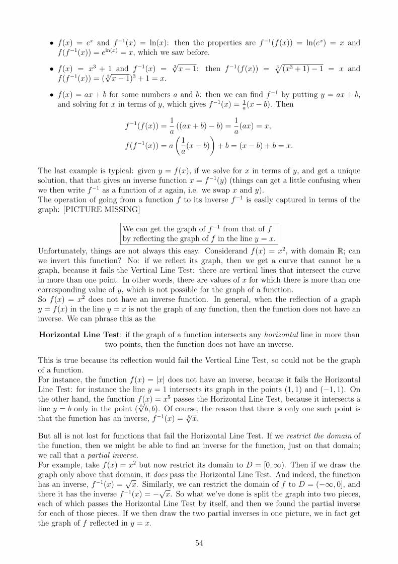
• f(x) = ex and f−1(x) = ln(x): then the properties are f−1(f(x)) = ln(ex) = x andf(f−1(x)) = eln(x) = x, which we saw before.

• f(x) = x3 + 1 and f−1(x) = 3√x− 1: then f−1(f(x)) = 3

√(x3 + 1)− 1 = x and

f(f−1(x)) = ( 3√x− 1)3 + 1 = x.

• f(x) = ax + b for some numbers a and b: then we can find f−1 by putting y = ax + b,and solving for x in terms of y, which gives f−1(x) = 1

a(x− b). Then

f−1(f(x)) =1

a((ax+ b)− b) =

1

a(ax) = x,

f(f−1(x)) = a

(1

a(x− b)

)+ b = (x− b) + b = x.

The last example is typical: given y = f(x), if we solve for x in terms of y, and get a uniquesolution, that that gives an inverse function x = f−1(y) (things can get a little confusing whenwe then write f−1 as a function of x again, i.e. we swap x and y).The operation of going from a function f to its inverse f−1 is easily captured in terms of thegraph: [PICTURE MISSING]

We can get the graph of f−1 from that of fby reflecting the graph of f in the line y = x.

Unfortunately, things are not always this easy. Considerand f(x) = x2, with domain R; canwe invert this function? No: if we reflect its graph, then we get a curve that cannot be agraph, because it fails the Vertical Line Test: there are vertical lines that intersect the curvein more than one point. In other words, there are values of x for which there is more than onecorresponding value of y, which is not possible for the graph of a function.So f(x) = x2 does not have an inverse function. In general, when the reflection of a graphy = f(x) in the line y = x is not the graph of any function, then the function does not have aninverse. We can phrase this as the

Horizontal Line Test: if the graph of a function intersects any horizontal line in more thantwo points, then the function does not have an inverse.

This is true because its reflection would fail the Vertical Line Test, so could not be the graphof a function.For instance, the function f(x) = |x| does not have an inverse, because it fails the HorizontalLine Test: for instance the line y = 1 intersects its graph in the points (1, 1) and (−1, 1). Onthe other hand, the function f(x) = x5 passes the Horizontal Line Test, because it intersects aline y = b only in the point ( 5

√b, b). Of course, the reason that there is only one such point is

that the function has an inverse, f−1(x) = 5√x.

But all is not lost for functions that fail the Horizontal Line Test. If we restrict the domain ofthe function, then we might be able to find an inverse for the function, just on that domain;we call that a partial inverse.For example, take f(x) = x2 but now restrict its domain to D = [0,∞). Then if we draw thegraph only above that domain, it does pass the Horizontal Line Test. And indeed, the functionhas an inverse, f−1(x) =

√x. Similarly, we can restrict the domain of f to D = (−∞, 0], and

there it has the inverse f−1(x) = −√x. So what we’ve done is split the graph into two pieces,

each of which passes the Horizontal Line Test by itself, and then we found the partial inversefor each of those pieces. If we then draw the two partial inverses in one picture, we in fact getthe graph of f reflected in y = x.

54

A very important source of examples is trigonometry, for instance f(x) = sin(x). This functionfails the Horizontal Line Test miserably: y = sin(x) intersects the line y = 0 in infinitely manypoints! But again we can restrict the domain; the standard choice (which could have beenanything) is to take D = [−π

2, π

2], and then the range is R = [−1, 1]. Then we define

arcsin(x) = sin−1(x) with domain [−1, 1] and range[−π

2, π

2

],

This function does not have any simpler formula, we only know it as the inverse of sin(x). Soif we want to evaluate for instance arcsin 1

2, then we need to find an x between −π/2 and π/2

that gives sin(x) = 1/2: if we remember the table right, we know that sin(π/6) = 1/2, soarcsin 1

2= π

6.

See Stewart, 1.6 for pictures of these inverse trigonometric functions.Similarly, if we restrict cos(x) to the domain D = [0, π], then we can define the partial inverse

arccos(x) = cos−1(x) with domain [−1, 1] and range [0, π] ,

and if we restrict tan(x) to D = [−π/2, π/2] (i.e., we take the piece between two asymptotes),then it’s range is R = (−∞,∞), then we define

arctan(x) = tan−1(x) with domain (−∞,∞) and range[−π

2, π

2

].

When differentiating these functions in the next section, we’ll need the following identities:

cos(arcsin(x)) =√

1− x2

This is cos(θ) where θ is the angle such that sin(θ) = x. Since sin(θ) = opphyp

, draw a right

triangle with angle θ, hypotenuse 1 and opposite side x. Then since cos(θ) = adjhyp

= adj, we get

cos(θ) =√

1− x2, using Pythagoras.Similarly, we get

sin(arccos(x)) =√

1− x2

by drawing a triangle with angle θ = arccos(x), hypotenuse 1 and adjacent side x. Thensin(θ) = opp =

√1− x2.

Finally, we also need

cos(arctan(x)) =1√

1 + x2

In this case, θ = arctan(x) so x = tan(θ) = oppadj

. So draw the triangle with opposite side x and

adjacent side 1, then the hypotenuse is 1 + x2 by Pythagoras, so cos(θ) = adjhyp

= 1√1+x2

.

8.4 Derivatives of inverse functions

Having learned these new functions, we’d like to know how to differentiate them, so to know

d

dxf−1(x),

if we know f . This involves implicit differentiation.Write y = f−1(x), which by definition is equivalent to x = f(y) (a little confusing, but f−1

55

is the function we’re differentiating, so we take its variable to be x). Then differentiatinngx = f(y) on both sides gives

d

dxx =

d

dxf(y)

1 = f ′(y) · dydx

=⇒ dy

dx=

1

f ′(y)=

1

f ′(f−1(x)),

so we have what me might call the Inverse Function Rule:

d

dxf−1(x) =

1

f ′(f−1(x))

Do not misuse this as ddxf−1(x) = 1

f ′(x), that wouldn’t make sense because x is from the domain

of f−1(x), so might not be in the domain of f or f ′ at all, hence you shouldn’t be plugging xinto f ′.Let’s quickly test this on f−1(x) =

√x, so f(x) = x2 with domain [0,∞), and f ′(x) = 2x.

Then the rule givesd

dx

√x =

1

f ′(√x)

=1

2√x,

as we already learned. We can also test it on f−1(x) = ln(x), so f(x) = ex:

d

dxlnx =

1

f ′(ln(x))=

1

eln(x)=

1

x.

For the example f(x) = x3 + 1, f−1(x) = 3√x− 1 that we saw above we have

d

dx3√x− 1 =

1

3(f−1(x))2=

1

3( 3√x− 1)2

=1

3(x− 1)−2/3.

All of these we could of course already do, but for the inverse trigonometric functions we reallyneed it (unless we go through the implicit differentiation again, of course). With f(x) = sin(x),f ′(x) = cos(x) we get

f ′(f−1(x)) = cos(arcsin(x)) =√

1− x2,

using the identity cos(arcsin(x)) =√

1− x2, which we saw at the end of the last section. So

d

dxarcsin(x) =

1√1− x2

Similarly when f(x) = cos(x) we get

d

dxarccos(x) = − 1√

1− x2.

Finally, when f(x) = tan(x) and f ′(x) = 1cos2(x)

we have

f ′(f−1(x)) =11

(cos(arctan(x)))2

=1(11

1+x2

)2 =1

1 + x2,

sod

dxarctan(x) =

1

1 + x2.

56

Chapter 9

The Intermediate Value Theorem andthe Mean Value Theorem

9.1 Intermediate Values Theorem • 9.2 Mean Value Theorem

9.1 The Intermediate Value Theorem

The following theorem captures one of the most basic properties of continuous functions.

If f is a continuous function on [a, b], and d is a number between f(a)and f(b), then there is a number c in [a, b] such that f(c) = d.

In terms of the graph of f , this property is almost too simple: if (a, f(a)) is below the liney = N , and (b, f(b)) is above it, then if you draw the graph from one point to the other, youmust cross the line y = N , i.e. there is some point (c, f(c)) on that line.This theorem is important to mathematicians because it allows us to formally prove lots ofstatements about function that seem intuitively true. The point is that the formal definition ofcontinuity (which, remember, is just about limits and values of the function, not about drawingthe graph) is so general that continuous functions can do a lot of things that do not match ourintuitive idea of ’something you can draw without taking your pen off the paper’. For instancewe saw that functions involving sin

(1x

)can have weird properties, like having infinitely many

squiggles in a tiny piece of the graph, which is not something you do with a pen.Should you take more advanced math classes, you will see how theorems like this (and theMVT below) are used to build up a logically strict theory of functions, and how that will helpyou understand issues that don’t make sense intuitively. For now, though, we will merely use itto prove a few simple statements. Questions like these do show up on the exam for this course.Note that the conclusion of the theorem only says that some such number c exists, it gives youno clue about what it really is (other than the interval it is in). Nor does it say that this c isthe only such number, there could easily be several such c.

Roots of functions. A root of a function f(x) is a number c such that f(c) = 0.For instance, let f(x) = x4 + x− 3, which is certainly continuous. We can’t explicitly find

a root of this function (like we could for simpler functions like x2 − 4). Suppose we take a = 0and b = 2. Then f(0) = −3 and f(2) = 16 + 2 − 3 = 15. So N = 0 is between f(0) andf(2), hence by the Intermediate Value Theorem, there is a number c between 0 and 2 such thatf(c) = N = 0, i.e. a root of the function.

57

In general, to show that a function has a root in some interval, it is enough to find twonumbers a and b in that interval such that f(a) < 0 and f(b) > 0 (or the other way around).We can take the above example further. Since f(1) = 1 + 1− 3 < 0, and f(2) > 0, there is in

fact a root of f between 1 and 2. Similarly, f(11

2

)=(

32

)4+ 3

2− 3 =

(32

)4 − 32> 0, so there

is a root between 1 and 112. Next f

(54

)= 625

256+ 5

4− 3 = 625

256− 7

4= 625−64·7

4> 0, so the root is

between 1 and 114.

You see that we can keep going like this to get an approximation to a root of f (which in factis 1.164 · · · ). This is called the bisection method, because we keep cutting in half the intervalthat the root is in. It is nice in theory, but actually very inefficient; soon we will see that usinginformation from the derivative, we can approximate roots much, much faster (with Taylorpolynomials or Newton’s method).Of course, f might have more roots than just this one: indeed, since f(−2) = 16 − 2 − 3 > 0and f(0) < 0, there is another root somewhere in the interval [−2, 0]. And actually, we are notat all sure that there isn’t more than one root in these intervals.

Solutions to equations. A solution to an equation f(x) = g(x) is a number c such thatf(c) = g(c). Of course, this is nothing but a root of the function f(x)− g(x), so this is reallythe same thing, but it is good to know the distinction.Take for instance the equation cos(x) = x. Since for a = 0, we have cos(a) = 1 > 0 = aand for b = π/2, we have cos(b) = 0 < π/2 = b, there must be a solution to this equationbetween 0 and π/2. That follows from applying the Intermediate Value Theorem to the functionf(x) = cos(x)− x, which is continuous (on any interval) and has f(0) > 0 and f(π/2) < 0.Again we could approximate this solution by looking at cos(π/4) = 1/

√2 < π/4, so the solution

is between 0 and π/4. And we can go on like this, although evaluating cos and comparing thevalues gets harder (without a calculator).

9.2 The Mean Value Theorem

The mean value theorem is the big brother of the intermediate value theorem. In a similar way,it asserts the existence of some number c, but now instead of just continuous, the function hasto be differentiable.

If f is a differentiable function on [a, b], then there is a number c in[a, b] such that

f ′(c) =f(b)− f(a)

b− a.

Again, try to think of what this means in terms of the graph of f . The expression f(b)−f(a)b−a

(called a difference quotient) is the slope of the line between the two points (a, f(a)) and(b, f(b)), which are the endpoints of the graph above the interval [a, b]. Then the theorem saysthere is a point (c, f(c)) on the graph where the slope f ′(c) is exactly that difference quotient.In other words, a point on the graph where the slope of the graph is equal to the slope ofthe line between the endpoints of the graph. Or to look at it in another way, f(b)−f(a)

b−a is theaverage rate of change over the interval [a, b], and the theorem says there is a point where theinstantaneous rate of change equals the average rate of change.If you try some pictures, this should be pretty intuitive (though not as much as the IVT), butit may not be clear why this conclusion is useful. As it turns out, it is very useful, at least tomathematicians. Recall that the derivative f ′(a) is defined as the limit, as b goes to a, of the

difference quotient f(b)−f(a)b−a , but that doesn’t give us any kind of equation between values of

58

the derivative and of the function itself. That’s exactly what the MVT does: it gives a relationbetween the values of f on the endpoints of an interval [a, b] and the value of the derivative atsome number within that interval. Even if we don’t know what that number is exactly, we canstill deduce a lot of information about the function from its derivative.

Let’s see a simple example of how this works. Let f(x) =√x, and consider the interval [1, 2].

Then f is certainly differentiable there, so the Mean Value Theorem says there is a number cwith 1 ≤ c ≤ 2 such that

f ′(c) =f(2)− f(1)

2− 1=√

2− 1.

So the average slope over [1, 2] is√

2−1, and at some number in between, the slope f ′(c) of thegraph equals that graph. In fact, in this case we can find that c explicitly: since f ′(x) = 1

2√x,

we are looking for c such that

1

2√c

=√

2− 1 ⇒√c =

1

2(√

2− 1)⇒ c =

1

4(√

2− 1)2≈ 1.457,

so indeed there is such a c in that interval. This was possible because the function is prettysimple, and there is only one number c overall where the graph has this slope.

I should also show you an example where the conclusion fails. Take for instance f(x) = |x| onthe interval [−2, 2], where it is not differentiable at all values: there is a corner at x = 0. Thenf(2)−f(−2)

2−(−2)= |2|−|−2|

4= 0, but there is no c anywhere with f ′(c) = 0, because f ′(x) = −1 to the

left of 0 and f ′(x) = 1 to the right.So the differentiability condition is crucial.

The MVT has many more different applications than the IVT, and we will only see a few. Firstof all, it can provide formal proofs of many facts about differentiable functions that we havebeen using throughout this course, or that we’re about to see:

• If f ′(x) > 0, then f is increasing, and if f ′(x) < 0, then f is decreasing.

• If f ′′(x) > 0, then f is concave up, and if f ′′(x) < 0, then f is concave down.

• If F ′(x) = f(x), then all antiderivatives of f are of the form F (x) + c for a constant c.

• Taylor’s inequality

You can find these proofs in the book, but let me illustrate the first one. It seems easy to explainwhen you point at a picture (and that’s what I did earlier on in the class): if f ′(x) > 0, thenthe tangent line has positive slope, so is going up, hence the graph must be going up, right?Well, mathematicians are never happy when an argument about functions involves ’pointing ata picture’, because that picture can never represent all the possibilities. It clearly works for thetypical graph that you would draw, but does it also work for graphs involving sin

(1x

)? And

even if it does, how do we know that there are no other functions where crazy things happen?This is why we want to use the MVT to give a formal proof. So, suppose f ′(x) > 0 on some

interval [a, b]. Then by the MVT, there is a c in [a, b] such that f ′(c) = f(b)−f(a)b−a . Therefore

f(b) − f(a) = f ′(c)(b − a), and f ′(c)(b − a) > 0 since both f ′(c) > 0 and b − a > 0. Sof(b)− f(a) > 0, i.e. f(b) > f(a), which exactly means that f is increasing from a to b.

I will list the different types of questions involving the MVT that you may encounter.

59

Roots of functions. We can often use the MVT to show that some root is unique. Forinstance, let f(x) = x3 − x − 1. Then f(1) = −1 and f(2) = 5, so by the IVT f has at leastone root in [1, 2]. But to show that there isn’t more than one root in that interval, we need theMVT.Suppose there were at least 2 roots, let’s say f(a) = 0 and f(b) = 0, with a and b in [1, 2] anda < b. Then the MVT says there is c in [a, b] such that (with f ′(x) = 3x2 − 1)

3c2 − 1 =f(b)− f(a)

b− a= 0,

so 3c2 = 1 and c =√

1/3. But√

1/3 < 1 is not in the interval [1, 2], so something must bewrong: the assumption that there were at least two roots must be false, hence there is at mostone.

Bounded derivative ⇒ bounded function. Suppose we know that 3 ≤ f ′(x) ≤ 5 for allvalues of x. Then we can bound, for instance, the difference between f(2) and f(8): by the

MVT, there is a c such that f ′(c) = f(8)−f(2)8−2

, so f(8)− f(2) = 6f ′(c). Since 3 ≤ f ′(c) ≤ 5, weget that 18 ≤ f(8)− f(2) ≤ 30. And this is true for any function whose derivative is boundedlike that.

Inequalities between functions. We can also use the MVT to prove inequalities like

sin(x) < x for all x > 0.

This is obvious when x > 1, since then sin(x) ≤ 1 < x. So suppose x ≤ 1. Then there is a cbetween 0 and x so that (since d

dxsin(x) = cos(x))

cos(c) =sin(x)− sin(0)

x− 0=

sin(x)

x,

so since cos(c) < 1 (for 0 < x ≤ 1) we have sin(x)x

< 1, hence sin(x) < x.Another example is

ex > x+ 1 for all x 6= 0.

Let x be any nonzero number, then the MVT gives c in the interval [0, x] or [x, 0] (whichevermakes sense) such that

ec =ex − e0

x− 0=ex − 1

x.

If x > 0, then ec > 1, and multiplying through by x gives ex − 1 = ec · x > x, so we getex > x+ 1.If x < 0, then ec < 1, so ex − 1 = ec · x > x, since x is negative and ec < 1. Hence we getex > x+ 1 for all x 6= 0.

60

Chapter 10

Maclaurin Series and Taylor Series

10.1 Polynomial approximation • 10.2 Maclaurin polynomials • 10.3 Maclaurin series • 10.4 Comput-

ing with Maclaurin series • 10.5 Limits with Maclaurin series • 10.6 Taylor polynomials and series •10.7 Taylor’s Inequality and error estimation

10.1 Polynomial approximation

Recall that the linear approximation to a function f(x) around a = 0 is given by

T1(x) = f(0) + f ′(0)x

Why I renamed L(x) to T1(x) will become clear soon. Because this is the function whose graphy = T1(x) is the tangent line to y = f(x) at x = 0, this seems to be the best approximation tof(x) by a linear function. But what if we try to approximate f(x) using a quadratic functionax2 + bx+ c, or using a polynomial of higher degree? That’s what this chapter is about.Another way to look at it is that T1(x) is the easiest function that has T1(0) = f(0) andT ′1(0) = f ′(0). This makes sense because f(0) and f ′(0) are the most basic pieces of informationabout f around 0, so if we want to approximate f there, why not try to imitate f by makinga new function with just those two pieces of information.Then the next step would be to find the easiest function that has T2(0) = f(0) and T ′2(0) = f ′(0),and also T ′′2 (0) = f ′′(0). That should look like

T2(x) = f(0) + f ′(0)x+ ax2,

since then T2(0) = f(0) and T ′2(0) = f ′(0) already work; the quadratic term doesn’t changethat since it and its derivative are zero at x = 0. Then we can determine a by taking the secondderivative:

T ′2(x) = f ′(0) + 2ax, T ′′2 (x) = 2a,

so if we want T ′′2 (0) = f ′′(0), we should take a =f ′′(0)

2, which gives us the quadratic approxi-

mation to f(x) at a = 0:

T2(x) = f(0) + f ′(0)x+f ′′(0)

2x2

For instance, let f(x) = ex. If you use the linear approximation T1(x) = e0 + e0x = 1 +x to approximate e0.1 = 1.10517 · · · , you get T1(0.1) = 1.1. But if we use the quadraticapproximation T2(x) = e0 + e0x+ e0

2x2 = 1 + x+ x2

2, we get

T2(0.1) = 1 + 0.1 +0.01

2= 1.105,

61

which is a better approximation.Similarly, to approximate

√99.7 = 9.98498873 · · · we can take the function f(x) =

√100 + x

and use the linear approximation T1(x) = 10+ 120x, which gives T1(−0.3) = 10−3/200 = 9.985,

pretty good. But using f ′′(x) = ddx

12(x+100)−1/2 = −1

4(x+100)−3/2, so f ′′(0) = −1

4· 1√

1003 = −1

4000,

we get the quadratic approximation

T2(x) = 10 +1

20x− 1

8000x2,

which gives the approximation T2(−0.3) = 10 − 3/200 − 18000

9100

= 9.98498875; that’s muchbetter.

Before we go even further, a little notation: we define f (n)(x) to be the n-th derivative of f(x).So f (1) = f ′, f (2) = f ′′, f (3) = f ′′′, etc, and also f (0) = f itself.

Now let’s find the cubic approximation (a cubic is a polynomial of degree 3). It should look like

T3(x) = f(0) + f ′(0)x+f ′′(0)

2x2 + bx3,

and we want to have T(3)3 (0) = T ′′′3 (0) = f (3)(0). Since

T(1)3 (x) = f ′(0) + f ′′(0)x+ 3bx2, T

(2)3 (x) = f ′′(0) + 6bx, T

(3)3 = 6b,

to get T(3)3 (0) = f (3)(0), we should choose b = f (3)(0)

6, so the cubic approximation is

T3(x) = f(0) + f ′(0)x+ +f ′′(0)

2x2 +

f (3)(0)

6x3

Let’s apply this cubic approximation to the two examples above. For f(x) = ex we getT3(x) = 1 + x + x2

2+ x3

6, which gives an approximation to e0.1 = 1.10517 · · · of T3(0.1) =

1 + 0.1 + 0.01/2 + 0.001/6 ≈ 1.105167, again an improvement.For f(x) =

√x we get f (3)(x) = d

dx−14

(x + 100)−3/2 = 38(x + 100)−5/2, and f (3)(0) = 3

800000, so

the cubic approximation is

T3(x) = 10 +1

20x− 1

8000x2 +

3

6 · 800000x3,

which gives T3(−0.3) = 9.84988733125, which again is closer to√

99.7 = 9.98498873309 · · · .

10.2 Maclaurin polynomials

Just like we did above for n = 1, 2, 3, we can approximate a function around 0 by a polynomialTn(x) of any degree n. These polynomials are called Maclaurin polynomials. They are a specialcase of Taylor polynomials, which are approximations around some number a, which doesn’thave to be 0; we will get to those later, but I will focus on Maclaurin polynomials because theyare simpler, and if you understand those, Taylor polynomials are only one step further.The formulas we found for T2(x) and T3(x) generalize to the following formula for the Maclaurinpolynomial of degree n:

Tn(x) = f(0) + f ′(0)x+f (2)(0)

2!x2 +

f (3)(0)

3!x3 +

f (4)(0)

4!x4 + · · ·+ f (n)(0)

n!xn

62

Here n! stands for n · (n − 1) · (n − 2) · · · 2 · 1, so 1! = 1, 2! = 2 · 1 = 2, 3! = 3 · 2 · 1 = 6,4! = 4 · 3 · 2 · 1 = 24, etc. These factorials show up here because if you take g(x) = xn and youdifferentiate it n times, you get g′(x) = n · xn−1, g′′(x) = n · (n− 1) · xn−2, etc.So Tn(x) is constructed in such a way that Tn(0) = 0, T ′n(0) = f ′(0), T ′′n (0) = f ′′(0), and so on,

up to T(n)n (0) = f (n)(0), and that makes it a good approximation to f(x) around x = 0.

The easiest example to find the Maclaurin polynomials of is f(x) = ex, because f (n)(x) = ex,so f (n)(0) = 1 for all n. Therefore

Tn(x) = 1 + x+1

2!x2 +

1

3!x3 +

1

4!x4 + · · ·+ 1

n!xn.

We could use this to approximate numbers like e0.1 as closely as we want (although rightnow, to know how close we are, we need to know the actual value; soon we will see thatTaylor’s inequality solves this). Next week we will see Newton’s method, which is actuallyeven more efficient at approximating values than these polynomials. What’s special aboutthese polynomials is that they approximate the whole function on an interval; with Newton’smethod, to get approximations to different values, you need to do the same thing all over again,but once you have computed a Maclaurin polynomial, you can plug in any number (near 0),and you get your approximation.What’s more, they also have lots of theoretical applications. For instance, we do not yet knowhow to evaluate limits like

limx→0

ex − 1

x,

where plugging in gives an undefined 00, and there is no algebraic simplification possible. But

what if we approximate ex in this limit by, say, T2(x) = 1 + x+ 12x2? Then we get

limx→0

(1 + x+ 12x2)− 1

x= lim

x→0

x+ 12x2

x= lim

x→0

1 + 12x

1= 1.

In fact, it is not hard to see that if you take T3(x) instead, or any higher degree Tn(x), thenthe same happens. So if you believe me when I say that as you take larger and larger n, youcan approximate ex as closely as you want by a Tn(x), then we must have

limx→0

ex − 1

x= 1.

If you don’t believe me, wait till we learn about Taylor’s Inequality, then we will be able toprove this.

This approach in fact lets you compute pretty much any limit you could think of, except maybeones with |x| or some other non-differentiable function (makes sense because then you can’tcompute f (n)(0)). Before we do more of this, I’ll go one step further and introduce Maclaurinseries, which will allow us to skip over this approximation argument when doing limits this way,and that will make the computations a bit easier.

10.3 Maclaurin series

This section may seem a bit mysterious, and with good reason, because it uses some mathe-matics that will not be covered in this course at all. You can tell from the fact that in thebook, this material comes at the end of chapter 11, and we don’t treat anything from the first9 sections of that chapter. Nevertheless, if you’re able to suspend your disbelief, this is a very

63

useful simplification of the ideas around Maclaurin (and Taylor) polynomials, and it is a sneakpeak at some deeper mathematics.Above we saw that we could approximate functions and their values with Maclaurin polynomi-als, and higher degree polynomials give better approximations. What if we could instead use’polynomials’ of infinite degree? Would they be ’infinitely close’, i.e. exactly right? Amazingly,yes. We call that the Maclaurin series of a function:

f(x) = f(0) + f ′(0)x+f (2)(0)

2!x2 +

f (3)(0)

3!x3 + · · ·+ f (n)(0)

n!xn +

f (n+1)(0)

(n+ 1)!xn+1 + · · ·

This says that around 0, the function f is equal, not just approximately equal, but equal, tothe thing on the right. The thing on the right is a ’series’, an infinite sum of functions.To see that an infinite sum can even make sense, think of

2 = 1 +1

2+

1

4+

1

8+

1

16+ · · · .

So an infinite sum of numbers can be equal to something finite. Apparently, it is even possiblefor an infinite sum of functions to be finite for every number you plug in (from some interval),since that’s what the equation for the Maclaurin series above says.Another way to think of it is that limn→∞ Tn(x) = f(x), i.e. if you ’let the n in Tn(x) go toinfinity’, you get exactly f(x).There are two important aspects that I’ve ignored here:

• First of all, this only makes sense if f is infinitely differentiable at 0, i.e. if f (n)(0) existsfor any n. Luckily, this is the case for many functions we know, like ex and sin(x).

• Second, it may not work for all x, but possibly only for an interval around 0, and thenoutside that interval, the series does not equal a finite number at all. Whether or not itdoes will again depend on Taylor’s Inequality. The first example we will see that onlyworks on a restricted interval is 1

1−x

The basic example is again ex, whose Maclaurin series is

ex = 1 + x+1

2x2 +

1

3!x3 +

1

4!x4 + · · · .

We could also describe this series by saying that its ’general term’ is 1n!xn. This one is in fact

correct for any x, so for instance

e = e1 = 1 + 1 +1

2+

1

3!+

1

4!+

1

5!+ · · · .

Let’s find the Maclaurin series of sin(x). Then

f ′(x) = cos(x), f (2)(x) = − sin(x), f (3)(x) = − cos(x), f (4)(x) = sin(x), . . . ,

so

f ′(0) = cos(0) = 1, f (2)(x) = − sin(0) = 0, f (3)(x) = − cos(0) = −1, f (4)(x) = sin(0) = 0, . . . ,

and if we wanted to, we could keep going with this list, because it repeats itself every foursteps. Hence in the Maclaurin series for sin(x), the even powers of x all drop out, and the oddones alternately have a minus or not:

sin(x) = x− 1

3!x3 +

1

5!x5 − 1

7!x7 +

1

9!x9 + · · · .

64

This one also works for all x, so we magically get all kinds of series, like

1√2

= sin(π/4) =π

4− 1

3!

π3

43+

1

5!

π5

45− · · ·

Who knew√

2 and π were related?

To get the Maclaurin series of cos(x), we could do similar computations, but instead we will usea nice trick. Since d

dxsin(x) = cos(x), the Maclaurin series for cos(x) should be the derivative

of the Maclaurin series for sin(x), and we can compute that term by term. So

d

dxx = 1,

d

dx

−1

3!x3 = − 3

3 · 2 · 1x2 = − 1

2!x2,

d

dx

1

5!x5 =

1

4!x4, etc,

which gives us

cos(x) = 1− 1

2!x2 +

1

4!x4 − 1

6!x6 +

1

8!x8 + · · · .

Note that differentiating this again would give the Maclaurin series for − sin(x) (and look backat ex: you can see that its Maclaurin series is its own derivative!).

Finally let’s do one that doesn’t work for all x, but only on some interval around 0. I’ll justgive it, and you could check the derivatives f (n)(0) yourself. It is

1

1− x= 1 + x+ x2 + x3 + x4 + x5 + · · · , only on (−1, 1).

It makes sense that this doesn’t hold for all x, because for instance for x = 1, 11−x is not defined.

What’s more, if you plug in x = 2, then f(2) = −1, but the series would be 1+2+4+8+16+· · · ,which surely can’t be finite, because each term is larger than the last. In fact, for any x with|x| ≥ 1, we would get a series with each term larger than the previous one, which can nevergive a finite number.As a little trick to see this equality, try multiplying the right side by 1− x, then we get

(1−x)(1+x+x2 + · · · ) = (1−x)+(1−x) ·x+(1−x) ·x2 + · · · = 1−x+x−x2 +x2−x3 + · · · ,

and since every term other than 1 gets cancelled, this equals 1.

10.4 Computing with Maclaurin series

We’ve seen how to compute the coefficients in Maclaurin series using repeated derivatives, butthat is often a lot of work. Fortunately, we can compute a lot of them by reducing them tothe four basic ones we saw above (in this course, those four are the only ones that you shouldknow by heart). Here are some examples:

e3x = 1 + (3x) +1

2!(3x)2 +

1

3!(3x)3 + · · · = 1 + 3x+

9

2!x2 +

27

3!x3 + · · ·

sin(x2)

x2=

1

x2·(

(x2)− 1

3!(x2)3 +

1

5!(x2)5 − · · ·

)= 1− 1

3!x4 +

1

5!x8 − · · ·

1

1 + x=

1

1− (−x)= 1 + (−x) + (−x)2 + (−x)3 + · · · = 1− x+ x2 − x3 + · · ·

x

1 + x2= x · 1

1− (−x2)= x · (1 + (−x2) + (−x2)2 + (−x2)3 + · · · ) = x− x3 + x5 − x7 + · · ·

65

With some more clever trickery, we can find the Maclaurin series of ln(1 + x). Note that ln(x)does not exists at 0, so ln(x) has no Maclaurin series itself; the Maclaurin series for ln(1 + x)is actually a Taylor series for ln(x) around x = 1 in disguise.We can use that

d

dxln(1 + x) =

1

1 + x= 1− x+ x2 − x3 + · · · .

Then it’s not hard to see what Maclaurin series has this as a derivative: it must be

ln(1 + x) = x− 1

2x2 +

1

3x3 − 1

4x4 + · · · .

Because the Maclaurin series for 11−x only works on (−1, 1), the same is true of this one.

10.5 Limits with Maclaurin series

Now that we know about Maclaurin series, limit computations like we did above become a loteasier:

limx→0

ex − 1

x= lim

x→0

(1 + x+ x2 + · · · )− 1

x= lim

x→0

x+ x2 + · · ·x

= limx→0

1 + x+ · · ·1

= 1.

We only have to write down as many of the terms in the Maclaurin series as we need, since weknow what happens to the rest.I will give a few examples that hopefully speak for themselves. You should check first thatplugging in actually gives 0

0!

limx→0

sin(x)

x= lim

x→0

x− 13!x3 + · · ·x

= limx→0

1− 13!x2 + · · ·1

= 1

limx→0

sin(mx)

sin(nx)= lim

x→0

(mx)− 13!

(mx)3 + · · ·(nx)− 1

3!(nx)3 + · · ·

= limx→0

m− 13!

(mx)2 + · · ·n− 1

3!(nx)2 + · · ·

=m

n

limx→0

cos(2x)− ex2

x2= lim

x→0

(1− 12!

(2x)2 + 14!

(2x)4 − · · · )− (1 + (x2) + (x2)2 + · · · )x2

= limx→0

(−1

24− 1

)x2 + ( 1

4!24 − 1)x4 + · · ·

x2= −1

24− 1 = −3.

10.6 Taylor Polynomials and series

We saw that Maclaurin polynomials give approximations to functions around 0. Taylor polyno-mials are the more general version of Maclaurin polynomials, and they approximate functionsaround a, for some number a.The formulas for Taylor polynomials are basically the same as for Maclaurin polynomials, ex-cept that instead of writing them as a polynomials in x, we write them as polynomials in x−a,because then it will be easier to plug in values close to a. For example, the Taylor polynomialof degree 2 for f(x) =

√x around a = 25 looks like

T2(x) = 5 +1

10(x− 25)− 1

1000(x− 25)2.

This gives an approximation to√

26 of 5 + 110· 1 − 1

1000· 12 = 5.099. If we had multiplied out

this polynomial, plugging in 26 would have been much more work.

66

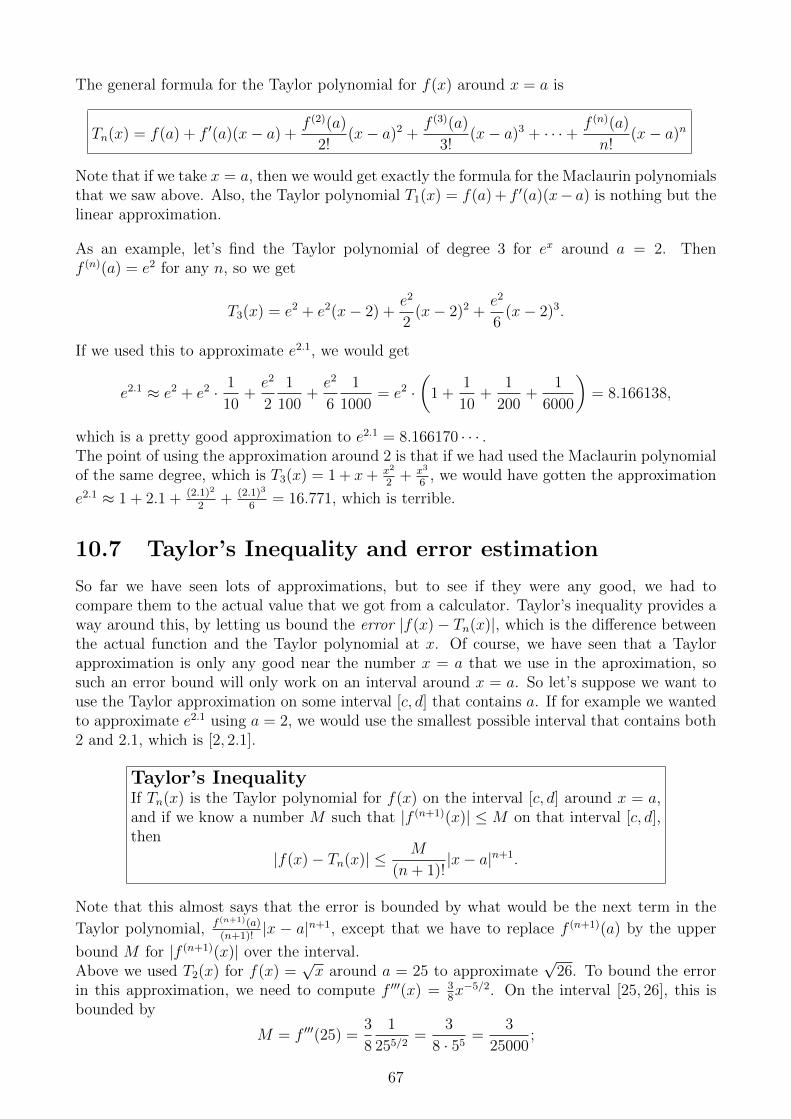
The general formula for the Taylor polynomial for f(x) around x = a is

Tn(x) = f(a) + f ′(a)(x− a) +f (2)(a)

2!(x− a)2 +

f (3)(a)

3!(x− a)3 + · · ·+ f (n)(a)

n!(x− a)n

Note that if we take x = a, then we would get exactly the formula for the Maclaurin polynomialsthat we saw above. Also, the Taylor polynomial T1(x) = f(a) + f ′(a)(x− a) is nothing but thelinear approximation.

As an example, let’s find the Taylor polynomial of degree 3 for ex around a = 2. Thenf (n)(a) = e2 for any n, so we get

T3(x) = e2 + e2(x− 2) +e2

2(x− 2)2 +

e2

6(x− 2)3.

If we used this to approximate e2.1, we would get

e2.1 ≈ e2 + e2 · 1

10+e2

2

1

100+e2

6

1

1000= e2 ·

(1 +

1

10+

1

200+

1

6000

)= 8.166138,

which is a pretty good approximation to e2.1 = 8.166170 · · · .The point of using the approximation around 2 is that if we had used the Maclaurin polynomialof the same degree, which is T3(x) = 1 + x+ x2

2+ x3

6, we would have gotten the approximation

e2.1 ≈ 1 + 2.1 + (2.1)2

2+ (2.1)3

6= 16.771, which is terrible.

10.7 Taylor’s Inequality and error estimation

So far we have seen lots of approximations, but to see if they were any good, we had tocompare them to the actual value that we got from a calculator. Taylor’s inequality provides away around this, by letting us bound the error |f(x)− Tn(x)|, which is the difference betweenthe actual function and the Taylor polynomial at x. Of course, we have seen that a Taylorapproximation is only any good near the number x = a that we use in the aproximation, sosuch an error bound will only work on an interval around x = a. So let’s suppose we want touse the Taylor approximation on some interval [c, d] that contains a. If for example we wantedto approximate e2.1 using a = 2, we would use the smallest possible interval that contains both2 and 2.1, which is [2, 2.1].

Taylor’s InequalityIf Tn(x) is the Taylor polynomial for f(x) on the interval [c, d] around x = a,and if we know a number M such that |f (n+1)(x)| ≤ M on that interval [c, d],then

|f(x)− Tn(x)| ≤ M

(n+ 1)!|x− a|n+1.

Note that this almost says that the error is bounded by what would be the next term in the

Taylor polynomial, f (n+1)(a)(n+1)!

|x − a|n+1, except that we have to replace f (n+1)(a) by the upper

bound M for |f (n+1)(x)| over the interval.Above we used T2(x) for f(x) =

√x around a = 25 to approximate

√26. To bound the error

in this approximation, we need to compute f ′′′(x) = 38x−5/2. On the interval [25, 26], this is

bounded by

M = f ′′′(25) =3

8

1

255/2=

3

8 · 55=

3

25000;

67

this is because the function x−5/2 is decreasing, so the maximum on [25, 26] occurs at 25.Hence Taylor’s Inequality with a = 25, x = 26 and n = 2 gives

|√

26− T2(26)| ≤ 3/25000

3!|26− 25|3 =

1

50000= 0.00002.

And indeed, the true error is

√26− T2(26) = 5.0990195− 5.099 = 0.0000195,

which is less that 0.00002.

We can also use Taylor’s inequality to estimate the error in a linear approximation. For instance,if we approximate e−0.1 with the linear approximation T1(x) = 1+x we got T1(−0.1) = 0.9. Weuse Taylor’s inequality with a = 0, n = 1 on the interval [−0.1, 0], so we can take M = e0 = 1(now since the function is increasing, we plug in the right endpoint of the interval). Then

|e−0.1 − T1(−0.1)| ≤ M

2!| − 0.1− 0|2 =

1

2(0.1)2 =

1

200= 0.005.

Therefore we know that e−0.01 is between 0.9 − 0.005 = 0.895 and 0.905, without having useda calculator (with a calculator we would get 0.9048 · · · ).

Another typical approach is to ask for an approximation that has error less than some number.For instance, we could ask for an approximation to e−0.1 that has an error of less than 0.0000001(so the linear approximation is not good enough). Then we have to find the n such that theerror bound for Tn is less than 0.0000001, so with M = 1 as above we need

0.0000001 ≥ M

n!| − 0.1− 0|n+1 =

1

n! · 10n+1.

For n = 2, this is 16·1000

, not good enough yet, for n = 3 this is 124·104

= 0.000004 · · · , still notquite good enough, and finally for n = 4 we get 1

120·105= 0.00000008 · · · , which will do.

So we have to use T4(x) = 1 + x+ 12x2 + 1

3!x3 + 1

4!x4, which gives

T4(−0.1) = 1− 1

10+

1

200− 1

6000+

1

240000= 0.9048375,

and with a calculator we would get e−0.1 = 0.904837418036 · · · , so the true error is indeed

0.000000082 · · · < 0.0000001.

68

Chapter 11

Antiderivatives & Substitution

11.1 Antiderivatives • 11.2 Substitution

11.1 Antiderivatives

• Reminder about DerivativesFirst I’ll remind you of a few derivatives that we’ll be using a lot:

(xn)′ = nxn−1,

(sinx)′ = cosx, (cosx)′ = − sinx, (tanx)′ = sec2 x,

(secx)′ = secx tanx, (sin−1 x)′ =1√

1− x2, (tan−1 x)′ =

1

x2 + 1,

(ex)′ = ex, (ln |x|)′ = 1

x

• About (ln |x|)′ = 1x

The last one deserves some extra attention, since this will show up again and again in integra-tion.You may only remember the derivative (ln x)′ = 1

x; this is of course correct, but is only true for

x in the domain of lnx, so for x > 0. For x ≤ 0, lnx doesn’t exist, and so a derivative wouldn’tmake sense.We can (and should) extend this differentiation formula to negative x by taking ln |x| instead.Think of the graphs: ln x only has a graph to the right of the y-axis, while ln |x| also has themirror image of the same graph to the left of the y-axis. We do have to actually check that thederivative is still 1/x for x < 0, which we do as follows:

x < 0 ⇒ |x| = −x ⇒ (ln |x|)′ = (ln(−x))′ =1

−x· (−1) =

1

x.

• AntidifferentiationAntidifferentiation (or ’taking the derivative’) is doing differentiation in reverse: given a functionf(x), find a function F (x) such that F ′(x) = f(x). This F (x) is then called an antiderivativeof f(x).Here are a few examples of important antiderivatives that you can obtain by reversing thedifferentiation formulas above:

f(x) = xn −→ F (x) =1

n+ 1xn+1 ( for n 6= −1),

69

f(x) = sinx −→ F (x) = − cosx, f(x) = cos x −→ F (x) = sinx,

f(x) = 1x2+1

−→ F (x) = tan−1 x, f(x) = 1√1−x2 −→ F (x) = sin−1 x

f(x) = ex −→ F (x) = ex, f(x) = 1x−→ F (x) = ln |x|

• ExamplesJust like with differentiation, we can combine these basic antiderivatives into more complexones. I will give a few examples first, and then explain some of the steps. Note that anantiderivative is easily checked: just differentiate it and see if you get the orginal function back.But I won’t do that in this writeup.

f(x) = 3x7 − 5 sin(x) −→ F (x) = 3 · 18· x8 − 5 · (− cos(x)) = 3

8x8 + 5 cos(x),

f(x) = e3x + 2√1−x2 + 1 −→ F (x) = 1

3e3x + 2 sec(x) + x,

f(x) = sin(2x− 3) −→ F (x) = −12

cos(2x− 3),

f(x) = (3x+ 7)5 + 1x+1

−→ F (x) = 16(3x+ 7)6 · 1

3+ ln |x+ 1| = 1

18(3x+ 7)6 + ln |x+ 1|

• ’Compensating’There is one informal trick that I used here several times; let me explain it for sin(2x− 3). Wecan guess that an antiderivative should involve − cos(2x − 3), but if we differentiate that, wewould get 2 sin(2x− 3) (with the 2 coming from the chain piece (2x− 3)′), which is not quitewhat we want. However, we can fix it by ’compensating’ for the 2 by putting a 1

2in front of

− cos(2x− 3). And indeed, then it works:(−1

2cos(2x− 3)

)′= −1

2· (− sin(2x− 3) · 2) = sin(2x− 3).

In general, if you know that F (x) is an antiderivative for f(x), then it’s easy to get one forf(ax+ b): you compensate for the a with 1

a, and you get 1

aF (ax+ b).

In the next section we will see a more systematic method that also includes this trick, but oftenit might be easier to do it this way.

• A function has infinitely many antiderivativesAbove I intentionally said ’an’ antiderivative instead of ’the’ antiderivative, because any functionhas many, in fact infinitely many, antiderivatives.To see this, consider f(x) = 2x. We can easily guess one antiderivative, F (x) = x2. ButG(x) = x2 + 1 is also a derivative: (x2 + 1)′ = 2x+ 0 = 2x. And so is x2 − 17, etc.In general, if F (x) is an antiderivative of f(x), then there are infinitely many antiderivatives ofthe form F (x) + C, for some constant C, and there are no others.

• Indefinite IntegralA bit of notation: we will write

∫f(x)dx for the ’general antiderivative’ F (x) + C of f(x),

where C is a constant.For example:∫

4x2dx =4

3x3 + C,

∫e−5xdx =

−1

5e−5x + C,

∫1

x− 2dx = ln |x− 2|+ C.

We call∫f(x)dx the indefinite integral of f(x), and then we call f(x) the integrand of the

integral. Evaluating an integral is called integration.

• Antidifferentiation RulesIn differentiation, we had lots of rules that let us differentiate combinations of functions. In

70

antidifferentiation, there aren’t nearly as many rules; the ones we’ve used above are: the sumrule, the constant mutiple rule, and a rule for compositions of functions where the inner functionis a linear function (ax+ b):∫

(f(x) + g(x)) dx =∫f(x)dx+

∫g(x)dx∫

af(x)dx = a∫f(x)dx∫

f(ax+ b)dx = 1aF (ax+ b) + C, if F (x) is an antiderivative of f.

However, for integrals there is in general no product rule for∫f(x)g(x)dx, no quotient rule for∫ f(x)

g(x)dx, and no chain rule for

∫f(g(x))dx.

Unlike for differentiation, where every function has a derivative and we have the rules to find it,for antidifferentiation there will be many functions that we won’t be able to find an antideriva-tive for.

11.2 Substitution

• Turning the chain rule aroundAs I said, for integration there is no analog to the chain rule, in the sense of a formula for∫f(g(x))dx. However, we do get a formula by simply turning the chain rule around:∫

f ′(g(x)) · g′(x)dx = f(g(x)).

Of course, this won’t be nearly as useful as a formula for∫f(g(x))dx would have been, but it

will have to do.To apply to this to an integral, we’ll have to identify a g and an f such that the integrand lookslike f ′(g(x)) · g′(x). This may involve some guessing.◦ For instance, to evaluate

∫2x cos(x2)dx we can guess g′(x) = 2x, and then deduce the rest:

g′(x) = 2x ⇒ g(x) = x2 ⇒ f ′(g(x)) = cos(g(x)) ⇒ f ′(x) = cos(x) ⇒ f(x) = sin(x),

=⇒∫

2x cos(x2)dx = f(g(x)) = sin(x2) + C.

◦ Here’s a harder one: ∫cos(x)

sin(x)dx.

We can see the integrand as 1sin(x)

· cos(x), and then guess g′(x) = cos(x), and deduce:

g′(x) = cos(x) ⇒ g(x) = sin(x) ⇒ f ′(g(x)) =1

g(x)⇒ f ′(x) =

1

x⇒ f(x) = ln |x|,

=⇒∫

cos(x)

sin(x)dx = f(g(x)) = ln | sin(x)|+ C.

• Substitution (aka change of variables)We can do the above trick more systematically, in several steps. Basically, we guess what theinner function g(x) is, then change variables to u = g(x), turning the integral into one in termsof u, which will hopefully be simpler.I will show the steps for the example

∫2x cos(x2)dx:

71

• Substitute u = x2.

• Replace dx by du, using dudx

= 2x⇒ du = 2xdx.

• Solve the resulting∫f(u)du.

• Write in terms of x again, using u = x2.

It will look like this:∫2x cos(x2)dx

u=x2=

∫cos(u) · (2xdx)

du=2xdx=

∫cos(u)du = sin(u) + C = sin(x2) + C.

• Examples◦ Let’s do ∫

x2(x3 + 1)7dx.

If we pick u = x3, then dudx

= 3x2, so du = 3x2dx. There’s no 3 in the integrand, so it will beeasier to use 1

3du = x2dx. Then∫

x2(x3+1)7dxu=x3=

∫(u+1)7(x2dx)

13du=x2dx

=1

3

∫(u+1)7du =

1

3·18

(u+1)8+C =1

24(x3+1)8+C.

◦ Let’s do a slightly harder one: ∫ex

(ex)2 + 1dx.

If we pick u = ex, then du = exdx, and we get:∫ex

(ex)2 + 1dx =

∫1

u2 + 1· (exdx) =

∫1

u2 + 1du = arctan(u) + C = arctan(ex) + C.

• How to choose u?To apply the substitution method, first the integrand should look like a product of two functions.Then the ’smaller’ (or ’simpler’) of those two might be your g′(x) = u′, and if you know anantiderivative of that one, then that will be your g(x) = u. If you recognize this u inside the’bigger’ function, that’s a good sign. But you’ll have to try and see what comes out.I’m not saying this always works; there are plenty of exceptions, though for the examples we’veseen so far it works. When this does fail, you’ll have to try choosing u to be any smaller functionthat you see inside another one. For example, if the ’bigger’ function is tan(

√x+ 2), you can

try u = x+ 2 or u =√x+ 2; either might work.

So to summarize:

• Write your integrand as a product of a ’smaller’ and a ’bigger’ function;

• Let u′ be the smaller function, antidifferentiate it to get u, and try substituting that;

• If the above fails, try choosing u to be any inner function.

There is often more than one choice for u. In the first of the two examples above, we couldhave used u = x3 + 1, then 1

3du = x2dx again, and you get∫

x2(x3 + 1)7dx =1

3

∫u7du =

1

3· 1

8u8 + C =

1

24(x3 + 1)8 + C,

72

just like before.It’s important to make sure that after you substituted u and du, the x is really gone. Otherwisethe substitution is useless, like in this example:∫

2x sin(x2 + x+ 1)dx =

∫sin(u+ x+ 1)du = ???

This is a common mistake. (In this example, I don’t think there is an antiderivative.)

• More examples◦ Let’s apply this to ∫ √

tan(x)− 3 sec2(x)dx.

The integrand is a product of√

tan(x)− 3 and sec2(x), the ’smaller’ one is sec2(x), and weknow (from page 1) an antiderivative for that: tan(x), which does indeed show up in the ’bigger’factor. So we choose u = tan(x), which implies du = sec2(x)dx, and we can work it out:∫ √

tan(x)− 3 · (sec2(x)dx) =

∫ √u− 3du =

1

3/2(u− 3)3/2 + C =

2

3(tan(x)− 3)3/2 + C.

◦ Let’s try ∫cos(ln |x|)

xdx.

To see it as a product of a ’smaller’ and a ’bigger’ function, we should write the integrand ascos(ln |x|) · 1

x. That should lead us to try u′ = 1

x, which implies u = ln |x|. In the ’bigger’

function we can recognize this u inside cos(x). So let’s substitute u = ln |x|, with du = 1xdx:∫

cos(ln |x|)x

dx =

∫cos(ln |x|) ·

(1

xdx

)=

∫cos(u)du = sin(u) + C = sin(ln |u|) + C.

• Manipulating firstYou will see many integrals where there doesn’t seem to be a possible substitution right away.Often you will have to do some kind of manipulation of the integrand, by algebra, trigonometryor exponential/logarithmic formulas, to get it into a form where you can do a substitution (orsome other method that we’ll learn later). In the last section of this chapter I will remind youof some of the trig or exponential identities that you might have to use.

◦ For example, consider ∫(x+ 1)2

xdx.

You can see this as a product in several ways, but none will lead to a useful substitution.However, a little algebra will make the integral easy (and we won’t even need substitution):∫

(x+ 1)2

xdx =

∫x2 + 2x+ 1

xdx =

∫ (x2

x+

2x

x+

1

x

)dx

=

∫xdx+

∫2dx+

∫1

xdx =

1

2x2 + 2x+ ln |x|+ C.

◦ A different kind of example is ∫1

x2 + 9dx.

73

This should make you think of∫

1x2+1

dx = arctan(x) +C, except that the 9 is in the way. Butyou can fix that with some algebra:

1

x2 + 9=

1

9· 1x2

9+ 1

=1

9· 1(

x3

)2+ 1

.

But now there’s a 3 – why is that better? Because you can substitute it away, using u = x/3,du = 1

3dx, 3du = dx:∫1

x2 + 9dx =

1

9

∫1(

x3

)2+ 1

dx =1

9

∫1

u2 + 1· 3du =

3

9arctan(u) + C =

1

3arctan

(x3

)+ C.

◦ Another one: ∫1

ex + e−xdx.

It’s hard to guess what to do. But maybe (maybe) it reminds you of one we did earlier, namely∫ex

(ex)2+1dx. And we can turn it into that one:

1

ex + e−x=ex

ex· 1

ex + e−x=

ex

(ex)2 + ex · e−x=

ex

(ex)2 + 1.

So we can do it with the substitution u = ex, like before:∫1

ex + e−xdx =

∫ex

(ex)2 + 1dx =

∫1

u2 + 1du = arctan(u) + C = arctan(ex) + C.

◦ Now consider ∫x+ 1

x− 1dx.

One way to do this is with the substitution u = x − 1: then du = dx, and to get rid of the xin the numerator we can plug in x = u+ 1 (which we get by rewriting u = x− 1):∫

x+ 1

x− 1dx =

∫x+ 1

udu =

∫(u+ 1) + 1

udu =

∫u+ 2

udu

=

∫ (u

u+

2

u

)du =

∫1du+

∫2

udu = u+ 2 ln |u|+ C1 = x− 1 + 2 ln |x− 1|+ C1.

But we can also do this one without a substitution, if we use the following algebra trick:∫x+ 1

x− 1dx =

∫(x− 1 + 1) + 1

x− 1dx =

∫x− 1

x− 1+

2

x− 1dx

=

∫1dx+

∫2

x− 1dx = x+ 2 ln |x− 1|+ C2.

That was a little easier.But wait! They’re different: the first has x − 1, the second x. But this is okay, it just meansthat the C’s are different, which is why I’ve given them different names. If for C2 we plug inC2 = C1 − 1, the second result becomes the same as the first.◦ Here’s a harder example that has two fairly different choices for u, neither of which is easilyrecognizable: ∫

x√x− 2

dx.

The ’smaller’ function would be x, but if u′ = x then u = 12x2, and we can’t substitute that.

So we’ll have to try any of the smaller functions that occurs inside. There are 2 and it turnsout they both work:

74

◦ First we’ll use u = x− 2, so du = dx. Then we’ll have to use x = u+ 2 to get rid of thex: ∫

x√x− 2

dx =

∫u+ 2√udu

This is an integral we can do after a little algebra: u+2√u

= u√u

+ 2√u

= u1/2 + 2u−1/2.Using that we get:

=

∫u1/2du+ 2

∫u−1/2du =

1

3/2u3/2 + 2 · 1

1/2u1/2 + C

=2

3(x− 2)3/2 + 4(x− 2)1/2 + C.

◦ The other option is to take u =√x− 2, so 2du = 1√

x−2dx, and to get rid of x we can

solve for x = u2 + 2. Then∫x ·(

1√x− 2

dx

)= 2

∫(u2 + 2)du =

2

3u3 + 4u+ C

=2

3(x− 2)3/2 + 4(x− 2)1/2 + C.

• Using trig formulasAnother class of integrals is those where you have to first manipulate the integrand with sometrig identities, like:∫

tan(x)dx =

∫sin(x)

cos(x)dx

u=cos(x)=

∫1

u(sin(x)dx)

−du=sin(x)dx=

−∫

1

udu = − ln |u|+ C = ln | cos(x)|+ C.

That was just using the definition of tan, but here’s a common one where you need the identitysin2(x) = 1

2− 1

2cos(2x) to lower the exponent of sin:∫

sin2(x)dx =

∫ (1

2− 1

2cos(2x)

)dx =

∫1

2dx+

1

2

∫cos(2x)dx =

1

2x+

1

4sin(2x) + C.

We’ll see many more of these later.

• Exponentials with other basesWe also need to be able to deal with functions that involve exponentials to bases other thane, like 10x. Fortunately, with the identity ax = eln(a)x you can rewrite those in terms of anexponential to base e, and use the (easy) antiderivative that you know for ex.For instance,∫

10xdx =

∫ (eln(10)

)xdx =

∫eln(10)xdx =

1

ln(10)eln(10)x + C =

1

ln(10)10x + C.

Note that ln(10) is just a number, so∫eln(10)xdx works just like

∫e3xdx = 1

3e3x + C.

Of course we can make them a little more complicated:∫2√x

√xdx

u=√x

=

∫2u(

1√xdx

)2du= 1√

xdx

= 2

∫2udu

75

= 2

∫eln(2)udu = 2 · 1

ln(2)eln(2)u + C =

2

ln(2)2√x + C.

• Trig & exponential identitiesHere I will remind you of a few formulas that you will often need in integration. You shouldalso be familiar with the graphs of all these functions; I won’t reproduce those here, but youcan find them in the book in sections 1.3, 1.4 and 6.7.First the fundamental identities for sin and cos:

sin2(x) + cos2(x) = 1, sin(2x) = 2 sin(x) cos(x), cos(2x) = cos2(x)− sin2(x).

I call these ’fundamental’ because you can derive all the other ones from them. For instance,plugging the first one into the third one in the form sin2(x) = 1− cos2(x) gives

cos(2x) = cos2(x)− (1− cos2(x)) = 2 cos2(x)− 1,

which gives us the following very useful formula for lowering the exponent of a cos; and I’ll alsogive the analogous one for sin, which is derived similarly:

cos2(x) =1

2+

1

2cos(2x), sin2(x) =

1

2− 1

2cos(2x).

Then there are the other trig functions, defined as follows:

sec(x) =1

cos(x), csc(x) =

1

sin(x),

tan(x) =sin(x)

cos(x), cot(x) =

1

tan(x)=

cos(x)

sin(x).

The only two identities for these that you might need are the ones that you get by dividingsin2(x) + cos2(x) = 1 by respectively cos2(x) and sin2(x):

tan2(x) + 1 = sec2(x), 1 + cot2(x) = csc2(x).

Finally, there’s inverse functions for all of these, but there aren’t many important identities forthose. The ones you’ll see most are arctan(x) = tan−1(x) and arcsin(x) = sin−1(x); occasionallyyou might see sec−1(x).

There are also some identities that you should know for ex and ln(x):

e0 = 1, ea+b = ea · eb, ea·b = (ea)b =(eb)a, e−a =

1

ea,

ln(1) = 0, ln(a · b) = ln(a) + ln(b), ln(ab) = b · ln(a), ln

(1

a

)= − ln(a).

The following two express that ex and ln(x) are inverse functions of one another:

eln(x) = x, ln(ex) = x.

These are particularly useful in dealing with exponentials to different bases:

7x =(eln(7)

)x= eln(7)·x,

as well as with those pesky tower functions (that have an x in both the base and the exponent):

xx =(eln(x)

)x= ex ln(x), (sin(x))cos(x) =

(eln(sin(x))

)cos(x)= ecos(x) ln(sin(x)).

76

Chapter 12

Definite Integrals

12.1 Definite integrals • 12.2 Fundamental Theorem of Calculus • 12.3 Substitution • 12.4 Riemann

sums

Note: There are no pictures in this chapter and the ones that follow, so often you’ll have todraw the relevant picture yourself (which shouldn’t be hard), or you’ll have to find a similarpicture in the book.

12.1 Definite integrals

• Temporary definition of definite integralWe define the new concept of a definite integral:∫ b

a f(t)dt is the net area under the graph of f(x) between a and b.

Several specifications should be made:

◦ ’under’ means between the graph and the x-axis.

◦ ’net’ area means that we count area above the x-axis positively, and we count area belowthe x-axis negatively.

◦ Normally a < b and we look at the area from left to right. If b < a, then the area shouldbe counted negatively, as if it’s going from right to left.

◦ Although we’re using the same symbol∫

as in the last chapter, right now these symbolshave nothing to do with each other: the indefinite integral

∫f(t)dt stands for the general

antiderivative of f , while∫ baf(t)dt is defined as an area.

◦ This definition is ’temporary’ because we’re not defining what area is; it’s an intuitivenotion, but in mathematics that’s not quite good enough. Later in this chapter we’ll seehow to define area and definite integrals precisely, using Riemann sums.

◦ The function f(t) inside is referred to as the integrand. The numbers a and b are thelimits of integration; a is the lower limit and b the upper limit.

• Properties of definite integralsWe can deduce several properties of definite integrals that we’ll need later.To begin with: ∫ a

a

f(t)dt = 0,

∫ a

b

f(t)dt = −∫ b

a

f(t)dt.

77

The first follows from the word ’between’ – there is no area between a and a. The secondcaptures the remark above that if you go from right to left instead of from left to right, thearea counts negatively.The next two properties describe what happens to a definite integral if you modify the integrand:∫ b

a

c · f(t)dt = c ·∫ b

a

f(t)dt,

∫ b

a

(f(t) + g(t)) dt =

∫ b

a

f(t)dt+

∫ b

a

g(t)dt.

The first says that the area under a scaled function equals the area under that function, scaledby the same factor. The second says that to calculate the area under the sum of two functionsyou can simply take the areas under the two functions separately, and add the two resultstogether. But note that this only makes sense if the two integrals have the same limits ofintegration.Both of these make perfect sense if you think of how areas work. Note that these happen toexactly match the properties of the indefinite integral

∫f(t)dt.

Finally, we can combine two integrals that have the same integrand but different limits ofintegration, but only in the special case where the upper limit of one integral is the lower limitof the other: ∫ b

a

f(t)dt+

∫ c

b

f(t)dt =

∫ c

a

f(t)dt.

Again this makes perfect sense if you look at the picture of such areas. But note that it onlyworks if the integrands really are the same.

• Examples using geometrySoon we’ll see a strong technique for evaluating definite integrals, but right now we can onlydo a few using area formulas that we know from geometry. For instance, when the integrand isa linear function, an area under the graph (a line) is a combination of rectangles and triangles.Another type that we can do is where the area is a half or quarter circle.Here are some examples of these.

◦ Let’s evaluate∫ 3

02xdx. If we draw the picture, we see that the area between 0 and 3 under

the graph is a triangle, with base 3 and height 2 · 3 = 6. Hence its area is 12· 3 · 6 = 9, so we

have∫ 3

02xdx = 9.

◦ Now we do∫ 2

−2(5 − 2x)dx. Again we draw the picture, and we see a triangle on top of a

rectangle. The rectangle is 4 by 1, so has area 4. The triangle is 4 by 8, so has area 16. Hencewe have

∫ 2

−2(2x+ 5)dx = 20.

◦ A different one is∫ 4

0(1− x)dx. Now the area consists of 2 triangles: one is 1 by 1 and above

the x-axis, the other is 3 by 3, but below the x-axis. As defined above, the second triangleshould be counted negatively, giving us

∫ 4

0(1− x)dx = 1

2· 1 · 1− 1

2· 3 · 3 = −4.

◦ We evaluate∫ 3

−3

√9− x3dx. The area is a half circle, with center at the origin, and radius

3. Hence the area of the whole circle would be π · 32, and the area of a half circle is 9π2

. So∫ 3

−3

√9− x3dx = 9π

2.

12.2 The Fundamental Theorem of Calculus

• Area FunctionsBy an area function of f we shall mean a function of the form

A(x) =

∫ x

a

f(t)dt.

78

This type of function will be important in the Fundamental Theorem that’s coming up.◦ As an example, consider A(x) =

∫ x0

(2t + 1)dt. Then when we draw the picture we can seethat A(0) = 0, A(1) = 2 (1 by 1 rectangle and a 1 by 2 triangle), and A(3) = 12 (3 by 1rectangle, 3 by 6 triangle).In fact, we can find a general formula: A(x) is the area of an x by 1 rectangle plus an x by(2x+ 1)− 1 = 2x triangle, which gives us A(x) = x+ 1

2· x · 2x = x2 + x.

You may notice that this is an antiderivative of A(x). The next theorem tells us that thisalways happens.

• Fundamental Theorem of Calculus (FTC)We have defined indefinite integrals (antiderivatives) and definite integrals (like area functions)in very different ways; we even used the same symbol. Of course, this was for a reason, whichis given by the Fundamental Theorem:

FTC: An area function of f is an antiderivative of f .

This is the short version; what we will most often make use of are the following two consequences(and especially of the first one), which together make up the long version:

◦∫ ba f(x)dx = F (b)− F (a), if F is an antiderivative of f , and f is continuous on [a, b]

◦ ddx

∫ xa f(t)dt = f(x)

There are different approaches as to what to call FTC: the book calls the two consequences theFTC, I prefer the short version above. Either way, these are just different versions of the sameidea, and it’s okay to refer to any of it as the FTC.In the first one, the restriction that f must be continuous on the interval [a, b] is important: ifthere is a discontinuity of f between a and b, then the formula might be wrong. We’ll see moreabout this later.

•Why?You can find a detailed proof of the FTC in the book; here I will give an outline of the idea,but first I’ll say why the consequences are consequences.◦ The second is just a restatement (if A(x) is an antiderivative of f(x), then f(x) is a derivativeof A(x)).◦ For the first consequence, take the area function A(x) =

∫ xaf(t)dt and let F (x) be any

antiderivative of f(x). Then we know that they only differ by some constant, so F (x) =A(x) + C. But then, since A(a) =

∫ aaf(t)dt = 0, we already have

F (b)− F (a) = (A(b) + C)− (A(a) + C) = A(b)− A(a) = A(b) =

∫ b

a

f(t)dt.

◦ To show that the FTC is true, we show that the derivative of A(x) =∫ xaf(t)dt is in fact

f(x). We’ll have to use the definition of derivative, which tells us

A′(x) = limh→0

A(x+ h)− A(x)

h.

With the sum property for definite integrals above we get

A(x+ h)− A(x) =

∫ x+h

a

f(t)dt−∫ x

a

f(t)dt =

∫ x+h

x

f(t)dt

79

By definition of the definite integral, this is the thin area under the graph of f(x) between xand x+h. Since in the limit h is going to zero, this strip gets thinner and thinner. Because it’sso thin, it’s pretty much a rectangle with width (x + h) − x = h and height f(x), so the areaof the strip will approach the area of the rectangle, which is width times height, h · f(x). Then

A′(x) = limh→0

A(x+ h)− A(x)

h= lim

h→0

h · f(x)

h= lim

h→0f(x) = f(x).

• Examples using∫ baf(x)dx = F (b)− F (a)

This is one of the most important tools in this course: to evaluate a definite integral, find anantiderivative F (x) of the integrand, and plug in the limits. Since we do not yet have thatmany techniques for finding antiderivatives (substitution is in the next section), I will only doa few examples here.One piece of notation: since the form F (b) − F (a) will occur a lot, and it might be annoyingto write out the F twice if it’s complicated, we will use a vertical bar like this:

F (b)− F (a) = F (x)∣∣∣ba.

The examples don’t require much explanation, I’ll just write down the solutions:∫ 2

1

x3dx =1

3x3∣∣∣21

=

(1

323

)−(

1

313

)=

8

3− 1

3=

7

3,∫ π

π/2

sin(x)dx = − cos(x)∣∣∣ππ/2

= (− cos(π))− (− cos(π/2)) = −(−1)− 0 = 1,∫ 2

−1

(x2 − 3x+ 2)dx =

(1

3x3 − 3

2x2 + 2x

) ∣∣∣2−1

=

(1

38− 3

24 + 2 · 2

)−(

1

3(−1)3 − 3

2(−1)2 + 2(−1)

)=

8

3− 6 + 4 +

1

3+

3

2+ 2 =

9

2.

• Examples using ddx

∫ xaf(t)dt = f(x)

This formula is usually pretty straightforward to use. Here are two examples:

d

dx

∫ x

2

t5dt = x5,

d

dx

∫ 3

x

e−t2

dt =d

dx

(−∫ x

3

e−t2

dt

)= − d

dx

∫ x

3

e−t2

dt = −e−x2 .

The second one used the property∫ ab

= −∫ ba

of definite integrals that we saw before.There is one tricky variation to this type of question, for instance

d

dx

∫ x3

0

sin(t)dt.

Here instead of an x in the limit of integration, we have a function of x. So this is a compositionF (G(x)) with the outer function F (x) =

∫ x0

sin(t)dt and the inner function G(x) = x3. To

80

differentiate a composition like that, we use the chain rule, ddxF (G(x)) = F ′(G(x)) ·G′(x). We

know that G′(x) = 3x2, and we can also do

F ′(x) =d

dx

∫ x

0

sin(t)dt = sin(x).

Hence we haved

dx

∫ x3

0

sin(t)dt = F ′(G(x)) ·G′(x) = sin(x3) · 3x2.

12.3 Substitution

We’ve seen how to use substitution for indefinite integrals, but for definite integrals there is atwist to how the limits are plugged in. There are two ways to do this:

(A) Work out the integral with substitution, return to x, and then plug in the limits.

(B) Adjust the limits to the substitution, and plug them in without having to return to x.

I’ll explain this in a few examples.

◦ I’ll do the integral

∫ 3

2

2x sin(x2)dx both ways, with the substitution u = x2, du = 2xdx:

(A) :

∫ 3

2

2x sin(x2)dx =

∫ x=3

x=2

sin(u)du = − cos(u)∣∣∣x=3

x=2= − cos(x2)

∣∣∣32

= − cos(9) + cos(4).

The important thing here is to make clear that the limits 2 and 3 should not be plugged in foru, but for x. So to write

∫ 3

2sin(u)du would have been very wrong, because it would mean that

you’re going to plug in u = 2 and u = 3.For method (B), we write the limits in terms of u = x2:

x = 2⇒ u = 22 = 4, x = 3⇒ u = 32 = 9,

and use that to adjust the limits:

(B) :

∫ 3

2

2x sin(x2)dx =

∫ 9

4

sin(u)du = − cos(u)∣∣∣94

= − cos(9) + cos(4).

In general method (B) is slightly more efficient, but it’s important to understand both ways(and even more important not to confuse them).

◦ Question: Find the net area under the graph of ln(x)x

on the interval [e, e2].The net area is given by the definite integral∫ e2

e

ln(x)

xdx.

I’ll use method (B). The substitution to use is

u = ln(x), du =1

xdx,

so the limits become

x = e ⇒ u = ln(e) = 1,

x = e2 ⇒ u = ln(e2) = 2.

Then we get ∫ e2

e

ln(x)

xdx =

∫ 2

1

udu =1

2u2∣∣∣21

=1

2

(22 − 12

)=

3

4.

81

12.4 Riemann sums

• Real definition of the definite integralAt the beginning of this chapter I gave a ’temporary’ definition of the definite integral, whichdepended on an intuitive sense of what area is. Now I will introduce the real definition, andthen I will explain what the components of the formula mean.∫ b

a

f (x)dx = limn→∞

n∑k=1

f (xk)∆x,

where xk = a+ (k − 1) · b− an

, ∆x =b− an

.

Note: The book uses slightly different notation in this definition. It writes lim∆→0

instead of

limn→∞

, xk instead of xk, and ∆xk instead of ∆x. You can use either notation.

• Approximating areas with rectanglesNote: you need to look at the relevant picture here – either the ones I showed you in class, orfor instance Figure 5.9 in the book.The definition above basically gives a formula for the area of a shape where one side can be’curvy’. The idea behind it is to fill up such an area with smaller shapes whose area we know(rectangles), and then adding the areas of those rectangles to get an approximation for thelarger area. By using more and more smaller and smaller rectangles, the approximation shouldget better and better, at least if we do it right.This can be done in general, but here we use a simple and systematic approach: we userectangles that all have the same width, and we match their heights to the graph. Let’s workout formulas for the resulting approximation, for a function f(x) on the interval [a, b].If we use n rectangles of equal width, we should divide the interval up into n equal parts, sothe width of a rectangle must be

∆x =b− an

.

Then the k-th rectangle will have its left side above

xk = a+ (k − 1) ·∆x = a+ (k − 1) · b− an

.

To see that there should be a k − 1 there, note that the first rectangle has its left side abovea = a+ 0 ·∆x, the second above a+ 1 ·∆x, etc.Then the height of each rectangle should match the height of the graph (at the left side of therectangle), so the height of the k-th rectangle should be f(xk).Finally we can write down the sum of the areas (width × height) of the rectangles, which isthe approximation for the area under the graph:

(f(x1) ·∆x) + (f(x2) ·∆x) + (f(x3) ·∆x) + · · ·+ (f(xn) ·∆x).

Such a sum is called a Riemann sum.• Sum notationFor convenience, we will write out Riemann sums using the summation symbol

∑, which is

defined byn∑k=1

f(k) = f(1) + f(2) + f(3) + · · ·+ f(n).

82

For example:5∑

k=1

k2 = 12 + 22 + 32 + 42 + 52,

3∑k=1

1

k + 1=

1

1 + 1+

1

2 + 1+

1

3 + 1.

• Refining the rectanglesSo the Riemann sum for f(x) on [a, b] with n rectangles is given by

n∑k=1

f(xk)∆x.

The only step left is to make the rectangles smaller and smaller, which you’ll have to believemakes the area approximation better and better. This is done by letting n get larger andlarger, which makes ∆x smaller and smaller, hence also the rectangles. This process is exactlydescribed by the limit limn→∞, so we have our whole definition:∫ b

a

f(x)dx = limn→∞

n∑k=1

f(xk)∆x,

where xk = a+ (k − 1) · b− an

, ∆x =b− an

.

• Different kinds of Riemann sumsAbove we chose to let the rectangle touch the graph with its top left corner. This is just achoice, we could also have chosen the top right corner, or even another point on the top edge,like the midpoint. These choices give different Riemann sums, and we name them as follows.

The sumn∑k=1

f(xk)∆x is called a

• left Riemann sum if xk = a+ (k − 1) · b−an

;

• right Riemann sum if xk = a+ k · b−an

;

• midpoint Riemann sum if xk = a+(k − 1

2

)· b−a

n.

I used left Riemann sums to define the definite integral, but I could just as well have used anyof the others, since the resulting limit has the same value. This is because as the rectangles getsmaller and smaller, it matters less and less which point of the top edge is on the graph.

• Questions you might be asked about Riemann sumsHere are the two main types of questions that you should be able to answer about Riemannsums.

◦ Write the right Riemann sum with n = 3 for∫ 4

2sin(x)dx.

We first compute the width and the xk:

∆x =4− 2

3=

2

3, xk = 2 + k · 2

3.

Then we write out the formula:

n∑k=1

f(xk)∆x =3∑

k=1

sin

(2 + k · 2

3

)· 2

3= sin

(2 +

2

3

)· 2

3+ sin

(2 +

4

3

)· 2

3+ sin (4) · 2

3.

83

◦ Identify the definite integral that this is a Riemann sum for:

limn→∞

n∑k=1

√1 +

3k − 3

n· 3

n.

This type of question is a bit like puzzling, you have to recognize the parts of the Riemann sumin it, and extract the f , the a and the b.In this case, it’s easy to guess that 3

nis the ∆x, so b−a

n= 3

nand b− a = 3.

Then√

1 + 3k−3n

should be f(xk), so a good guess seems to be xk = 1 + 3k−3n

= 1 + (k − 1) · 3n,

which makes sense because it has ∆x = 3n

in it. But now we can read off that a = 1, whichtogether with b − a = 3 gives b = 4. Finally, since we know what xk is, we also see thatf(x) =

√x.

Together this gives us the definite integral that the sum above is a left (because of the (k− 1))Riemann sum for: ∫ 4

1

√xdx.

Actually, we could also have chosen xk = 3k−3n

and f(x) =√

1 + x. Then a = 0, so b = 3, andthe integral we get as answer is ∫ 3

0

√1 + xdx.

This is also correct, and equivalent to the first integral, because we can obtain it by substitutingu = x+ 1 and adjusting the limits of integration accordingly.As you see, this type of question can have more than one correct answer.

84

Chapter 13

Integration by parts and other topics

13.1 Integration by parts • 13.2 Trigonometric integrals • 13.3 Odd and even functions • 13.4 Averages

and the MVT

13.1 Integration by parts

• Turning the product rule aroundEarlier we saw that there is no chain rule for integration, but that we can still turn the chainrule for differentiation around, which gave us the substitution method. Similarly, there is noproduct rule for integration, but we can still derive an integration rule from the product rulefor differentiation, as follows:

(uv)′ = u′v + uv′ =⇒ uv′ = (uv)′ − u′v

=⇒∫uv′dx =

∫(uv)′dx−

∫u′vdx

=⇒∫udv = uv−

∫vdu.

To get this last formula we used that dvdx

= v′, so v′dx = dv, and similarly u′dx = du; and weused that the integral of the derivative of uv is just uv, so

∫(uv)′dx = uv+C (and it’s okay to

leave out the C here, because there will be a C from the second integral anyway).This is the indefinite integral version; let’s right away give the definite integral version:∫ b

a

u(x)v′(x)dx = u(x)v(x)∣∣∣ba−∫ b

a

v(x)u′(x)dx.

Note that here we can’t use the du and dv notation, because it has to be clear that we’replugging in x = a and x = b.

A common mistake in using integration by parts for definite integrals is to forget the∣∣∣ba, i.e.

to just leave the u(x)v(x) in the answer. That’s clearly wrong, because the result of a definiteintegral cannot have an x in it.I will give several examples of applying this method, and then I will try to give a heuristic forchoosing the u and v, which is probably the hardest thing about this method.• Examples◦ Let’s do the integral

85

∫x cos(x)dx.

The choice for for u and dv to make here is:

u = x dv = cos(x)dxdu = dx v = sin(x)

So we have uv = x sin(x) and vdu = sin(x)dx, and we get

⇒∫x cos(x)dx = x sin(x)−

∫sin(x)dx = x sin(x) + cos(x) + C.

With integration by parts, it’s usually worth it to check your answer, so let’s differentiate it(with the product rule):

(x sin(x) + cos(x))′ = (x sin(x))′ + (cos(x))′ = (sin(x) + x cos(x))− sin(x) = x cos(x).

Here’s what the result will look like for a definite integral:∫ π

0

x cos(x)dx = (x sin(x) + cos(x))∣∣∣π0

= (π sin(π) + cos(π))− (0 + cos(0)) = (−1)− (1) = −2.

We see that doing integration by parts for definite integrals is not very different, since we cansimply do it for the indefinite integral first, and the plug in the limits.

◦ Let’s do∫

ln(x)

x2dx.

It’s harder to choose u and dv here, so let me write out several choices:

u = 1x2

dv = ln(x)dxdu = − 1

x3dx v =?

u = ln(x)x

dv = 1xdx

du = 1−ln(x)x2

dx v = ln |x|u = ln(x) dv = 1

x2dx

du = 1xdx v = − 1

x

We see right away that the first one is useless, since we can’t integrate ln(x) (yet).In the second one, dv does integrate nicely, and we can differentiate u, but then du is prettycomplicated. That’s not good, since we’d be getting an integrand vdu that’s uglier than theintegrand we started with.The third one looks better: we get uv = − ln(x)

xand vdu = 1

x· − 1

xdx = − 1

x2dx, and we get∫

ln(x)

x2dx = − ln(x)

x−∫− 1

x2dx = − ln(x)

x− 1

x+ C = − ln(x) + 1

x+ C .

Again, let’s check by differentiating (with the quotient rule):(− ln(x) + 1

x

)′= −(ln(x) + 1)′ · x− (ln(x) + 1) · (x)′

x2= −

1x· x− (ln(x) + 1)

x2=

ln(x)

x2.

• Choosing u and dvThere is no perfect strategy for choosing u and dv, but two guidelines are:

• u should become simpler when you differentiate it;

• dv should be easy to integrate.

86

This was clear for ln(x)x2

: we couldn’t integrate ln(x), so dv = ln(x)dx is not a good choice; andln(x)x

actually becomes more complicated when you differentiate, so u = ln(x)x

is also no good.But be aware that even when these conditions hold, it sometimes still doesn’t work...

• Examples◦ Let’s apply this to ∫

x sec2(x)dx.

If we choose u = x, then du = dx is very simple, and we can integrate dv = sec2(x)dx, since(tan(x))′ = sec2(x) so v = tan(x).No other choices would work: we can’t integrate sec(x) (yet), and sec2(x) does not have asimple derivative. In general, if the integrand is x times something more complicated, youshould always try u = x, since du = dx is one of the best simplifications that you can get: thex just goes away!To continue with the integral, with uv = x tan(x) and vdu = tan(x)dx we have∫

x sec2(x)dx = x tan(x)−∫

tan(x)dx.

As often happens, the integral we’re left with is simpler, but we’re not done yet. Luckily we’veseen this one before (in the substitution section), we have to use the definition of tan(x) first,and then substitute u = cos(x), du = − sin(x)dx:∫

tan(x)dx =

∫sin(x)

cos(x)dx = −

∫1

udu = − ln |u|+ C = − ln | cos(x)|+ C.

Then the integral is ∫x sec2(x)dx = x tan(x) + ln | cos(x)|+ C .

◦ Now consider ∫ln(x)dx.

The integrand doesn’t look like a product, but we could see it as the product of ln(x) and 1.We still don’t know how to integrate ln(x), but its derivative is nice and simple; and we doknow how to integrate 1.So let’s choose

u = ln(x) dv = 1 · dxdu = 1

xdx v = x

Then uv = x ln(x) and vdu = x · 1xdx = dx, so∫

ln(x)dx = x ln(x)−∫dx = x ln(x)− x+ C .

Let’s check that (it’s an important one – you might want to memorize it):

(x ln(x)− x)′ = (x ln(x))′ − (x)′ =

(1 · ln(x) + x · 1

x

)− 1 = ln(x).

• Repeated integration by partsNow consider ∫

x2exdx.

87

Since the derivative of x2 is a bit simpler and ex is easy to integrate, let’s try

u = x2 dv = exdxdu = 2xdx v = ex

Then uv = x2ex and vdu = 2xexdx, so∫x2exdx = x2ex − 2

∫xexdx.

This is not an overwhelming success, since∫xexdx is not very easy, but it is an improvement.

In fact, if we now apply integration by parts to∫xexdx, with the easy choice

u = x dv = exdxdu = dx v = ex

,

then uv = xex and vdu = exdx, and we can work out∫xexdx = xex −

∫exdx = xex − ex + C.

Putting these together we get∫x2exdx = x2ex − 2 (xex − ex) + C = (x2 − 2x− 2)ex + C .

• Repeat and solve for IA different type is ∫

e2x cos(x)dx.

A reasonable choice isu = e2x dv = cos(x)dx

du = 2e2xdx v = sin(x).

Then uv = e2x sin(x) and vdu = 2e2x sin(x), so∫e2x cos(x)dx = e2x sin(x)− 2

∫e2x sin(x)dx.

This doesn’t look like an improvement – it’s just like the one we started with! However, if wetry the new integral anyway, with the choice

u = e2x dv = sin(x)dxdu = 2e2xdx v = − cos(x)

,

then we get ∫e2x sin(x)dx = −e2x cos(x) + 2

∫e2x cos(x)dx.

We end up with the integral we started with! That may sound bad, but actually it’s a goodthing, because if we put them together, we get∫

e2x cos(x)dx = e2x sin(x)− 2

(−e2x cos(x) + 2

∫e2x cos(x)dx

)

= e2x sin(x) + 2e2x cos(x)− 4

∫e2x cos(x)dx.

88

So we have our original on both sides of the equation, which means we can solve for it. It’susually easiest to call the integral I, and solve for I:

I =

∫e2x cos(x)dx = e2x sin(x) + 2e2x cos(x)− 4I

=⇒ 5I = e2x sin(x) + 2e2x cos(x) + C =⇒ I =e2x

5(sin(x) + 2 cos(x)) + C.

13.2 Trigonometric integrals

In this section we will see how to deal with integrals of the forms∫sinm(x) cosn(x)dx,

∫tanm(x) secn(x)dx.

• Strategy for∫

sinm(x) cosn(x)dxHere are two special cases of this kind of integral where we can use a simple substitution:∫

sinm(x) cos(x)dxu=sin(x)

=

∫umdu =

1

m+ 1um+1 + C =

1

m+ 1sinm+1(x) + C,∫

cosn(x) sin(x)dxu=cos(x)

= −∫undu = − 1

n+ 1un+1 + C = − 1

n+ 1cosn+1(x) + C.

So when either cos(x) or sin(x) occurs to the power 1, the integral is easy. In the general case,our strategy will be to reduce it to (a combination of) these simpler integrals.We will do this reducing by using one of the following familiar trigonometric formulas:

sin2(x) = 1− cos2(x), sin2(x) =1

2− 1

2cos(2x),

cos2(x) = 1− sin2(x), cos2(x) =1

2+

1

2cos(2x).

Which one to use will depend on whether one of m and n is odd, or if both are even:

• If m is odd, we split off one sin(x), and in the remaining even power of sin(x)we substitute sin2(x) = 1 − cos2(x), to get a combination of integrals of the form∫

cosn(x) sin(x)dx.

• If n is odd, we can similarly split off one cos(x) and substitute cos2(x) = 1−sin2(x),to get integrals of the form

∫sinm(x) cos(x)dx.

• If both m and n are even, then we substitute sin2(x) = 12− 1

2cos(2x) and cos2(x) =

12

+ 12

cos(2x) whenever possible, and see what new integrals we get.

• Examples of∫

sinm(x) cosn(x)dx

◦∫

cos3(x)dx

Since there is an odd power of cos(x), we split off one cos(x) and substitute cos2(x) = 1−sin2(x):∫cos3(x)dx =

∫cos2(x) · cos(x)dx =

∫(1− sin2(x)) cos(x)dx

u=sin(x)=

∫(1− u2)du = u− 1

3u3 + C = sin(x)− 1

3sin3(x) + C.

89

◦∫

sin2(x)dx

There are no odd powers, so we use sin2(x) = 12− 1

2cos(2x):∫

sin2(x)dx =

∫ (1

2− 1

2cos(2x)

)dx =

1

2x− 1

4sin(2x) + C.

◦∫

sin4(x)dx

Again we use sin2(x) = 12− 1

2cos(2x), but now we’re not done right away:∫

sin4(x)dx =

∫(sin2(x))2dx

=

∫ (1

2− 1

2cos(2x)

)2

dx =

∫ (1

4− 1

2cos(2x) +

1

4cos2(2x)

)dx.

To integrate the third term, we need to separately use cos2(2x) = 12

+ 12

cos(4x) (which is theformula cos2(x) = 1

2+ 1

2cos(2x) with 2x plugged in for x):∫

1

4cos2(2x)dx =

∫ (1

8+

1

8cos(4x)

)dx =

1

8x+

1

32sin(4x) + C.

With this we can finish the main integral:∫sin4(x)dx =

∫ (1

4− 1

2cos(2x)

)dx+

∫1

4cos2(2x)dx

=

(1

4x− 1

4sin(2x)

)+

(1

8x+

1

32sin(4x) + C

)=

3

8x− 1

4sin(2x) +

1

32sin(4x) + C.

◦∫

sin5(x) cos2(x)dx

Since we have an odd power of sin(x), we split off one sin(x) and substitute sin2(x) = 1−cos2(x):∫sin5(x) cos2(x)dx =

∫(sin2(x))2 · cos2(x) · sin(x)dx =

∫(1− cos2(x))2 · cos2(x) · sin(x)dx

=

∫ (cos2(x)− 2 cos4(x) + cos6(x)

)· sin(x)dx

u=cos(x)= −

∫ (u2 − 2u4 + u6

)du

= −1

3cos3(x) +

2

5cos5(x)− 1

7cos7(x) + C.

• The integrals∫

tan(x)dx,∫

sec(x)dx, and∫

sec3(x)dxBefore attacking integrals like

∫tanm(x) secn(x)dx, we will first do some of the basic ones,

because these are not done with the general strategy.◦ We’ve seen the integral of tan(x) before, obtained by substituting u = cos(x):∫

tan(x)dx = ln | cos(x)|+ C.

◦∫

sec(x)dx is notoriously tricky, it’s very hard to come up with its solution. I’ll try to explainwhere it comes from, but if you find this hard to follow, this is one integral that’s worth

90

memorizing.The trick comes down to observing (out of the blue) that

(sec(x) + tan(x))′ = sec(x) tan(x) + sec2(x) = (sec(x) + tan(x)) · sec(x),

so the derivative of f(x) = sec(x) + tan(x) equals itself times sec(x), in other words

f ′(x) = f(x) · sec(x) ⇒ sec(x) =f ′(x)

f(x)=

d

dxln |f(x)|.

What we have here is sec(x) as the derivative of something else, so we know an antiderivative:∫sec(x)dx = ln | sec(x) + tan(x)|+ C.

◦ A related integral of this type that I should mention is∫

sec3(x)dx (note that∫

sec2(x)dx =tan(x) + C is easy). It requires integration by parts, with the following choice for u and dv:

u = sec(x) dv = sec2(x)dxdu = sec(x) tan(x)dx v = tan(x)

,

so we get uv = sec(x) tan(x) and vdu = sec(x) tan2(x), hence (using tan2(x) = sec2(x)− 1, seebelow)

I =

∫sec3(x)dx = sec(x) tan(x)−

∫sec(x) tan2(x)dx

= sec(x) tan(x)−∫

sec(x)(sec2(x)− 1

)dx

= sec(x) tan(x)−∫ (

sec3(x)− sec(x))dx = sec(x) tan(x)− I + ln | sec(x) + tan(x)|

⇒ I =1

2sec(x) tan(x) +

1

2ln | sec(x) + tan(x)|+ C.

Here we used the ”solve for I” trick that we encountered in the section on integration by parts.

• Strategy for∫

tanm(x) secn(x)dxFor integrals of the form

∫tanm(x) secn(x)dx there is a similar strategy to the one we used for∫

sinm(x) cosn(x)dx, although it differs in that it doesn’t work in all cases.Because the derivatives of tan(x) and sec(x) are

(tan(x))′ = sec2(x), (sec(x))′ = sec(x) tan(x),

we again have certain cases that can be done by a simple substitution:∫tanm(x) · sec2(x)dx

u=tan(x)=

∫umdu =

1

m+ 1tanm+1(x) + C,∫

secn(x) · (sec(x) tan(x))dxu=sec(x)

=

∫undu =

1

n+ 1secn+1(x) + C.

And again we try to do the other ones by reducing to these. For that we need the basic relationbetween tan(x) and sec(x), which we derive as follows:

sin2(x) + cos2(x) = 1 ⇒ sin2(x)

cos2(x)+

cos2(x)

cos2(x)=

1

cos2(x)⇒ tan2(x) + 1 = sec2(x).

There are now two cases where this approach works, but also one where it doesn’t:

91

• If n is even, we split off one sec2(x), substitute sec2(x) = tan2(x)+1 in the remainingpower of sec(x), to get a combination of integrals of the form

∫tanm(x) · sec2(x)dx;

• If m is odd and n ≥ 1, we split off sec(x) tan(x), substitute tan2(x) = 1− sec2(x)in the power of tan(x) that remains, to get a combination of integrals of the form∫

secn(x) · (sec(x) tan(x))dx;

• When neither of these conditions applies, we have to try something else.

• Examples for∫

tanm(x) secn(x)dx

◦∫

tan6(x) sec4(x)dx

We have an even power of sec(x), so we split off one sec2(x) and substitute sec2(x) = tan2(x)+1for the other:∫

tan6(x) sec4(x)dx =

∫tan6(x)(tan2(x) + 1) · sec2(x)dx =

∫ (tan8(x) + tan6(x)

)· sec2(x)dx

u=tan(x)=

∫(u8 + u6)du =

1

9tan9(x) +

1

7tan7(x) + C.

◦∫

tan5(x) sec7(x)dx

Now we have an odd power of tan(x), so we split off sec(x) tan(x) and then substitute tan2(x) =sec2(x)− 1 in the rest:∫

tan5(x) sec7(x)dx =

∫(sec2(x)− 1)2 sec6(x) · (sec(x) tan(x))dx

=

∫(sec10(x)− 2 sec8(x) + sec6(x)) · (sec(x) tan(x))dx

u=sec(x)=

∫(u10 − 2u8 + u6)du =

1

11sec11(x)− 2

9sec9(x) +

1

7sec7(x) + C.

13.3 Odd and even functions

• DefinitionA function f(x) is called:

• Even if f(−x) = f(x) for all x in the domain of f ;

• Odd if f(−x) = −f(x) for all x in the domain of f .

Some examples:f(x) = x2 is even because f(−x) = (−x)2 = x2 = f(x),

f(x) = x3 is odd because f(−x) = (−x)3 = −x3 = −f(x),

x6 −√

1− x2 is even because (−x)6 −√

1− (−x)2 = x6 −√

1− x2,

cos(x) is even because cos(−x) = cos(x),

sin(x) is odd because sin(−x) = − sin(x),

x sin(x) is even because (−x) sin(−x) = x sin(x),

tan(x) is odd because tan(−x) =sin(−x)

cos(−x)=− sin(x)

cos(x)= − tan(x),

Note: most function are neither odd nor even.• SymmetryThese two properties have clear meanings in terms of symmetry of the graph of the function:

92

• If f(x) is even, then its graph y = f(x) is symmetric in the y-axis.This means that if you reflect it in the y-axis, in other words you look at the graphy = f(−x), then that’s the same graph as y = f(x).

• If f(x) is odd, then its graph y = f(x) is symmetric in the origin.This means that if you reflect it in the y-axis and then in the x-axis, and get the graphy = −f(−x), then that’s the same graph as y = f(x).

• Integrals of odd and even FunctionsIf you know that a function is odd or even, then that can help you do some integrals of it,namely the ones that have symmetric limits like

∫ a−a. For even functions, the left part of the

graph will have the same area as the right part, so we only have to compute one and multiplyit by two. For odd functions, the left part of the graph will have the same area as the rightpart, but counted negatively, so the areas of the left and right part will cancel each other out,and the integral equals 0.

• If f(x) is odd and continuous on [−a, a], then

∫ a

−af(x)dx = 0.

• If f(x) is even and continuous on [−a, a], then

∫ a

−af(x)dx = 2

∫ a

0

f(x)dx.

The second one will merely make the calculation a bit more efficient (plugging in 0 is usuallyeasy), but the first one can make the entire calculation redundant.

A few examples of integrals of odd and even functions (check for yourself if the function is oddor even): ∫ 7

−7

x4dx = 2

∫ 7

0

x4dx = 2 · 1

5x5∣∣∣70

=2

5· (75 − 0) =

2

5· 75,∫ 1

−1

tan(x)dx = 0,

∫ 2

−2

x5 cos(x)dx = 0.

13.4 Averages and the Mean Value Theorem

• AveragesYou already know what a discrete average is: for instance, if f(k) gives your score on the k-thhomework, and there are n homeworks in total, then your average score is

f =1

n

n∑k=1

f(k).

This is called a discrete average because this is a discrete function, which means it only takesvalues on isolated numbers.In calculus however, we deal with functions that take values on all numbers in an interval [a, b],so we couldn’t take a sum like above. What we can do instead is take the integral over theinterval, and we divide by the length of the interval (similarly to dividing by n above). Thisgives the average value of a function:

f =1

b− a

∫ b

a

f(x)dx.

• Example◦ Suppose that the elevation (in km) of a hiking trail is given by

h(x) =1

10(2 + 6x− x2),

93

where x is the distance along the trail in km, running from x = 0 to x = 6. (This is actuallypretty much going up and down the Grouse Grind, if you know what that is...)Then the average elevation of the trail is

h =1

6− 0

∫ 6

0

1

10(2 + 6x− x2)dx =

1

60(2x+ 3x2 − 1

3x3)∣∣∣60

=1

60(12 + 108− 72) =

4

5.

So the average height of this trail is 800m.Why would this be useful? It’s in a way the best summary that you can give of the trailin a single number. And that’s useful because if you have two completely different trails, youcouldn’t really compare their elevation functions, but you can compare their average elevations.This is of course also why we compute the average of your grades at the end of a course!

• The Mean Value Theorem for integralsThe following fact about averages is called the Mean Value Theorem for integrals:

If f is a continuous function on [a, b], then there is a point c in [a, b] for which f(c) = f .

In other words, on an interval, there is always a point where the value of the function equalsits average value over that interval.

• Example◦ For the hiking trail example above, this theorem says that there should be a c in [0, 6] suchthat h(c) = h = 4

5. Because h(x) is simple enough, we can find this c algebraically:

4

5= h(c) =

1

10(2 + 6c− c2) ⇒ 40 = 10 + 30c− 5c2 ⇒ 5c2− 30c+ 30 = 0 ⇒ c2− 6c+ 6 = 0

=⇒ c =1

2

(6±√

36− 24)

= 3±√

3,

using the quadratic formula. So in fact there are two c, c = 3−√

3 ≈ 1.3 and c = 3+√

3 ≈ 4.7,as we would expect, since we go up and down the same trail.

94

Chapter 14

Trigonometric Substitution, PartialFractions, and Numerical Integration

14.1 Trigonometric substitution • 14.2 Partial fractions • 14.3 Numerical integration

14.1 Trigonometric substitution

• IntroductionWe do not yet know how to handle integrals involving variations of the functions

√1− x2,

√1 + x2,

√x2 − 1.

For instance, we cannot yet do integrals like∫ √1− x2dx,

∫1√

4 + x2,

∫x2

(2x2 − 3)3/2.

The basic observation that we need for solving these is that√1− sin2(θ)

∗= cos(θ),

√1 + tan2(θ)

∗= sec(θ),

√sec2(θ)− 1

∗= tan(θ).

I’ve put a ∗ over these equalities because they’re not quite true: the right hand sides should be| cos(θ)|, | sec(θ)|, and | tan(θ)|, since

√x2 = |x|, not x. But I’m going to ignore this for now,

and go into the finer details later.Here is why these equations help: to do for instance

∫ √1− x2dx, we can use the substitution

x = sin(θ) ⇒ dx = cos(θ)dθ

to get ∫ √1− x2dx =

∫ √1− sin2(θ) · (cos(θ)dθ) =

∫cos2(θ)dθ,

and this is a trigonometric integral that we can do.Note that this substitution is a bit different from the ones we’re used to: instead of somethinglike u = x2 when we see x2 in the integrand, we’re writing x = sin(θ), even though we don’tsee a sin(θ) in the integrand.Similarly, we can use the substitutions x = tan(θ), dx = sec2(θ)dθ to do∫ √

1 + x2dx =

∫ √1 + tan2(θ) · (sec2(θ)dθ) =

∫sec3(θ)dθ,

95

an integral we saw in the last chapter. And we can use x = sec(θ), dx = sec(θ) tan(θ)dθ for∫ √x2 − 1dx =

∫ √sec2(θ)− 1 · (sec(θ) tan(θ)dθ) =

∫tan2(θ) sec(θ)dθ,

which we can finish using tan2(θ) = 1− sec2(θ).

• Different forms of√

1− x2,√

1 + x2,√x2 − 1.

There are a number of different forms of these root functions for which we can use thesesubstitutions. I will illustrate these here without doing the integrals yet.For instance, for

√9− x2 we couldn’t use x = sin(θ) itself, but we can modify it to x = 3 sin(θ):

√9− x2

x=3 sin(θ)=

√32 − 32 sin2(θ) = 3

√1− sin2(θ) = 3 cos(θ).

Here are some examples of modified substitutions that work, with increasing difficulty:

√1 + 4x2

x= 12

tan(θ)=

√1 + 22 · (1/2)2 · tan2(θ) =

√1 + tan2(θ) = sec(θ),√

(x+ 1)2 − 25x=5 sec(θ)−1

=√

(5 sec(θ))2 − 52 = 5√

sec2(θ)− 1 = 5 tan(θ),

√2− 3x2

x=√

2√3

sin(θ)

=

√2− 3 · (

√2/√

3)2 sin2(θ) =√

2− 2 sin2(θ) =√

2 cos(θ).

• Examples of integrals

◦∫

1√1− x2

dx

We actually already know an antiderivative for the integrand, but it’s a good example, solet’s pretend we don’t know that antiderivative. Since we see a

√1− x2, we should use the

substitution x = sin(θ), dx = cos(θ)dθ, so∫1√

1− x2dx =

∫1√

1− sin2(θ)· cos(θ)dθ =

∫cos(θ)

cos(θ)dθ =

∫dθ = θ + C,

which is not the answer yet, because we have to return to x. To do that, we have to invert therelation x = sin(θ), which gives θ = sin−1(x). So the integral is what we thought it would be:∫

1√1− x2

dx = θ + C = sin−1(x) + C.

◦∫

1

(4x2 + 9)3/2dx

We use the substitution x = 32

tan(θ), dx = 32

sec2(θ), so∫1

(4x2 + 9)3/2dx =

∫1

(9 tan2(θ) + 9)3/2

(3

2sec2(θ)dθ

)=

3

2

∫sec2(θ)

93/2(sec2(θ))3/2dθ

=3

2 · 33

∫sec2(θ)

sec3(θ)dθ =

1

18

∫cos(θ)dθ = − 1

18sin(θ) + C.

To return to x, we invert x = 32

tan(θ) to get θ = tan−1(2x/3), which we plug in:

= − 1

18sin(tan−1(2x/3)) + C = − 1

18

2x/3√(2x/3)2 + 1

+ C = −1

9

x

3√

(2x/3)2 + 1+ C

96

= −1

9

x√4x2 + 9

+ C.

Here we used the identity sin(tan−1(x)) = x√x2+1

, which I will explain after the next integral.

◦∫ 6

3

√x2 − 9

xdx

We do the indefinite integral first, using the substitution x = 3 sec(θ), dx = 3 sec(θ) tan(θ)dθ:∫ √x2 − 9

xdx =

∫ √32 sec2(θ)− 32

3 sec(θ)(3 sec(θ) tan(θ)dθ) =

∫3 tan(θ)

3 sec(θ)(3 sec(θ) tan(θ)dθ)

= 3

∫tan2(θ)dθ = 3

∫(sec2(θ)− 1)dθ = 3 tan(θ)− 3θ + C.

To return to x, we invert x = 3 sec(θ) to get θ = sec−1(x/3), which we plug in:

= 3 tan(sec−1(x/3))− 3 sec−1(x/3) + C = 3√

(x/3)2 − 1− 3 sec−1(x/3) + C

=√x2 − 9− 3 sec−1(x/3) + C.

Here we used tan(sec−1(x)) =√x2 − 1, which I will explain now.

• Identities like sin(tan−1(x)) =x√x2 + 1

.

When doing trigonometric substitution integrals, you very often end up with formulas likesin(sin−1(x)), tan(sec−1(x), or sin(tan−1(x)). You have to simplify these using identities, butthere are too many different ones to memorize them, so you will have to know how to derivethem. There are two ways to do this: one is by ’reference triangle’, which the book does in 7.3;I’ll do the other method here because it doesn’t require a drawing.The easiest ones are

sin(sin−1(x)) = x, tan(tan−1(x)) = x, sec(sec−1(x)) = x.

The ones involving sec and tan we can reduce to the above using tan =√

sec2−1 and sec =√tan2 +1:

tan(sec−1(x)) =√

(sec(sec−1(x)))2 − 1 =√x2 − 1,

sec(tan−1(x)) =√

(tan(tan−1(x)))2 + 1 =√x2 + 1.

The ones with sin−1 inside we can do using tan = sincos

, sec = 1cos

, and cos =√

1− sin2:

tan(sin−1(x)) =sin(sin−1(x))

cos(sin−1(x))=

x√1− (sin(sin−1(x)))2

=x√

1− x2,

sec(sin−1(x)) =1

cos(sin−1(x))=

1√1− (sin(sin−1(x)))2

=1√

1− x2.

Finally, the ones with sin outside we can do as follows:

sin(tan−1(x)) =sin(tan−1(x))

cos(tan−1(x))· cos(tan−1(x))

1= tan(tan−1(x)) · 1

sec(tan−1(x))=

x√x2 + 1

,

sin(sec−1(x)) =sin(sec−1(x))

cos(sec−1(x))· cos(sec−1(x))

1= tan(sec−1(x)) · 1

sec(sec−1(x))=

√x2 − 1

x.

97

• The area of a circle!Let’s see an important application of this technique, namely the area of a circle. You alreadyknow what that is, of course, but you’ve probably never seen why.A circle with center at the origin and radius r is given by the equation x2 + y2 = r2, so thetop half of the circle is given by the function f(x) =

√r2 − x2. Then the area A of the circle

is given by 4 times the area of a quarter circle, which is given by the definite integral

A = 4

∫ r

0

√r2 − x2dx.

To compute this integral, we use the substitution x = r sin(θ), dx = r cos(θ)dθ. Here it’s easierto change the limits right away, using θ = sin−1(x/r): x = 0 gives θ = sin−1(0) = 0, x = r givesθ = sin−1(1) = π

2. Then

A = 4

∫ π/2

0

√r2 − r2 sin2(θ) · (r cos(θ)dθ) = 4r

∫ π/2

0

√r2 cos2(θ) cos(θ)dθ = 4r2

∫ π/2

0

cos2(θ)dθ

= 4r2

∫ π/2

0

(1

2+

1

2cos(2θ)

)dθ = 4r2

(1

2θ +

1

4sin(2θ)

) ∣∣∣π/20

= 4r2

((1

2· π

2+

1

4sin(π)

)− (0 + 0)

)= 4r2 · π

4= πr2.

• Completing the squareIn the examples above, underneath the square root we always had two terms, one with an x2

and one with a constant. But we can also deal with cases like√x2 + 2x+ 10, by completing

the square: √x2 + 2x+ 2 =

√x2 + 2x+ 1 + 1 =

√(x+ 1)2 + 1,

so we can use the substitution x = tan(θ)− 1 to simplify the integral∫ √x2 + 2x+ 2dx =

∫ √(x+ 1)2 + 1dx =

∫ √tan2(θ) + 1 sec2(θ)dθ =

∫sec3(θ)dθ.

In general, completing the square goes like this:

x2 + ax+ b =

(x2 + 2 · a

2x+

a2

4

)+

(b− a2

4

)=(x+

a

2

)2

+

(b− a2

4

)If this looks a bit mysterious, here’s the idea: we want x2+ax to look like (x+c)2 = x2+2cx+c2,so we take 2c = a, hence c = a

2, and then we compensate for the extra a2

4by subtracting it

from b.Here’s a harder example of an integral with completing the square:∫

1

(5 + 4x− x2)3/2dx =

∫1

(9− (x− 2)2)3/2dx

x=3 sin(θ)+2=

∫1

93/2(1− sin2(x))3/23 cos(θ)dθ

=1

9

∫cos(θ)

cos3(θ)dθ =

1

9

∫sec2(θ)dθ =

1

9tan(θ) + C =

1

9tan(sin−1((x− 2)/3)) + C

=1

9

x−23√

1−(x−2

3

)2+ C =

1

9

x− 2√9− (x− 2)2

+ C =1

9

x− 2√5 + 4x− x2

+ C.

98

• SubtletiesAs I warned at the start, I’ve been ignoring a subtlety here: since

√x2 = |x| (think of

√(−1)2 =

1 6= −1), I should have been writing√1− sin2(θ) =

√cos2(θ) = | cos(θ)|,

and similarly for the other ones. As it turns out, this is no problem for the sin and tansubstitutions, but for the sec things get a little tricky. To see how this works, we have to take acloser look at what values θ can take (its range); I’m assuming you’re familiar with the graphsof sin−1, tan−1, sec−1 (if not, look them up; see p.470 of the book).When we’re substituting x = sin(θ), we’re actually defining the new variable θ = sin−1(x), andthe range of sin−1(x) is −π/2 ≤ θ ≤ π/2. So in our manipulations, we’re are only dealingwith those θ. And luck has it that −π/2 ≤ θ ≤ π/2 happens to be an interval on whichcos(θ) is positive, which implies | cos(θ)| = cos(θ). So for the sin substitution, the formula√

1− sin2(θ) =√

cos2(θ) = cos(θ) is correct after all.Let me summarize it like this:

θ = sin−1(x) ⇒ − π

2≤ θ ≤ π

2⇒ cos(θ) ≥ 0 ⇒

√1− sin2(θ) = cos(θ).

For the tan substitution, the same thing happens (note that −π/2 and π/2 are not in the rangeof tan−1, because it has horizontal asymptotes there):

θ = tan−1(x) ⇒ − π

2< θ <

π

2⇒ sec(θ) ≥ 0 ⇒

√tan2(θ) + 1 = sec(θ).

However, for the sec substitution, something different happens. We’re defining θ = sec−1(x),but as you can see from the graph of that function, it has a weird range: it consists of twointervals, 0 ≤ θ < π/2 and π/2 < θ ≤ π. Similarly, its domain consists of two pieces, x ≤ −1and x ≥ 1. Because of this, there are actually two different sec substitutions, and which oneyou use depends on what values x takes (this is why integrals for which you need a secantsubstitution are usually given as definite integrals). The two cases look like this:

x ≤ −1 ⇒ π

2< θ ≤ π ⇒ tan(θ) < 0 ⇒

√sec2(θ)− 1 = | tan(θ)| = − tan(θ)

x ≥ 1 ⇒ 0 ≤ θ <π

2⇒ tan(θ) > 0 ⇒

√sec2(θ)− 1 = | tan(θ)| = tan(θ)

As if this isn’t hard enough, we usually substitute something like x = 3 sec(θ), so we’reactually dealing with θ = sec−1(x/3). That means we have to replace x ≥ 1 by x/3 ≥ 1 andx ≤ −1 by x/3 ≤ −1.Here are some examples that illustrate the sec-subtlety (we have respectively the cases x ≥ 1,x ≤ −1 and x/3 ≤ −1):∫ 2

1

√x2 − 1dx =

∫ x=2

x=1

√sec2(θ)− 1 · sec(θ) tan(θ)dθ =

∫ x=2

x=1

tan2(θ) sec(θ)dθ,

∫ −1

−2

√x2 − 1dx =

∫ x=−1

x=−2

√sec2(θ)− 1 · sec(θ) tan(θ)dθ = −

∫ x=−1

x=−2

tan2(θ) sec(θ)dθ,∫ −3

−4

√x2 − 9dx =

∫ x=−3

x=−4

√(3 sec(θ))2 − 32 · 3 sec(θ) tan(θ)dθ = − 9

∫ x=−3

x=−4

tan2(θ) sec(θ)dθ.

99

14.2 Partial fractions

• IntroductionA partial fraction decomposition of a rational function like 1

(x+1)(x+2)is a decomposition as a

sum of simpler fractions, like

1

(x+ 1)(x+ 2)=

1

x+ 1− 1

x+ 2.

If you read this from right to left, it is nothing but ”making common denominators”. But inthis direction it turns out to be very useful for integration, as in∫

1

(x+ 1)(x+ 2)dx =

∫ (1

x+ 1− 1

x+ 2

)dx

=

∫1

x+ 1dx−

∫1

x+ 2dx = ln |x+ 1| − ln |x+ 2|+ C.

We could also have done this integral with completing the square and a trigonometric substi-tution, but that would have been a lot more work. So by manipulating the integrand with alittle algebra first, we can make some such integrals a lot easier. We will also see integrals likethis that we can’t do any other way. But first we’ll need a systematic way of getting such apartial fraction decomposition.

• Partial fractions by matching coefficients◦ Here’s how we could obtain the decomposition above:

1

(x+ 1)(x+ 2)=

A

x+ 1+

B

x+ 2=A(x+ 2) +B(x+ 1)

(x+ 1)(x+ 2);

since the denominators are equal, the numerators should also be equal:

=⇒ 1 = A(x+ 2) +B(x+ 1) = (A+B)x+ (2A+B).

This means that we have two polynomials, 1 = 0 · x1 + 1 · x0 and (A + B)x + (2A + B) =(A+B)x1 +(2A+B)x0, that are equal; this means that the coefficient of corresponding powersof x must be equal:

=⇒ 0 = A+B, 1 = 2A+B.

These two equations in two unknowns are easy to solve: the first gives B = −A, and pluggingthat into the second gives

1 = 2A+ (−A) = A ⇒ A = 1, B = −A = −1.

Plugging those into the equation defining A and B gives us the decomposition.

◦ Let’s find the partial fraction decomposition for3

(x− 2)(3x+ 5).

We write3

(x− 2)(3x+ 5)=

A

x− 2+

B

3x+ 5=A(3x+ 5) +B(x− 2)

(x− 2)(3x+ 5)

Numerators equal: 3 = A(3x+ 5) +B(x− 2) = (3A+B)x+ (5A− 2B)

Match coefficients: 0 = 3A+B, 3 = 5A− 2B

Solve equations: B = −3A ⇒ 3 = 5A− 2(−3A) = 11A ⇒ A = 3/11,

B = −3A = −9/11.

100

So3

(x− 2)(3x+ 5)=

3

11

1

x− 2− 9

11

1

3x+ 5,

and we can compute the integral∫3

(x− 2)(3x+ 5)dx =

∫ (3

11

1

x− 2− 9

11

1

3x+ 5

)dx

=3

11

∫1

x− 2dx− 9

11

∫1

3x+ 5dx =

3

11ln |x− 2| − 9

11· 1

3· ln |3x+ 5|+ C

=3

11ln |x− 2| − 3

11ln |3x+ 5|+ C.

Notice the 1/3 in∫

13x+5

dx = 13

ln |3x + 5|; it’s a common mistake to forget about that in acalculation like this.

◦ Let’s find the partial fraction decomposition for2x+ 1

(x− 2)(x− 1).

2x+ 1

(x− 2)(x− 1)=

A

x− 2+

B

x− 1=A(x− 1) +B(x− 2)

(x− 2)(x− 1)

Numerators equal: 2x+ 1 = A(x− 1) +B(x− 2) = (A+B)x+ (−A− 2B)

Match coefficients: 2 = A+B, 1 = −A− 2B

Solve equations: B = 2− A ⇒ 1 = −A− 2(2− A) = A− 4 ⇒ A = 5,

B = 2− A = −3.

So2x+ 1

(x− 2)(x− 1)=

5

x− 2− 3

x− 1,

and the integral is∫2x+ 1

(x− 2)(x− 1)dx =

∫5

x− 2dx−

∫3

x− 1dx = 5 ln |x− 2| − 3 ln |x− 2|+ C.

• Partial fractions by plugging in rootsThe method above is the most natural, but now we will see an alternative method that is alittle faster.◦ It starts in the same way; for example for 1

(x+1)(x+2), we again set

1

(x+ 1)(x+ 2)=

A

x+ 1+

B

x+ 2=A(x+ 2) +B(x+ 1)

(x+ 1)(x+ 2),

and we set the numerators equal:

1 = A(x+ 2) +B(x+ 1).

But then we plug in the roots of the linear factors (x = −1 is the root of x + 1, x = −2 thatof x+ 2) to simply pick out the A and B:

Plug in x = −1: 1 = A · (−1 + 2) +B · 0 = A ⇒ A = 1,

Plug in x = −2: 1 = A · 0 +B · (−2 + 1) = −B ⇒ B = −1.

101

We get the same A and B as before. The trick here is that by plugging in a root, the corre-sponding linear factor becomes 0, taking the A or the B out of the equation, and leaving theother easy to read off.

◦ Let’s do this forx+ 1

x(2x+ 3).

x+ 1

x(2x+ 3)=A

x+

B

2x+ 3=A(2x+ 3) +Bx

x(2x+ 3)

Numerators equal: x+ 1 = A(2x+ 3) +Bx

Plug in x = 0: 0 + 1 = A · (0 + 3) +B · 0 = 3A ⇒ A =1

3

Plug in x = −32: − 3

2+ 1 = A · 0 +B · −3

2⇒ B =

(−2

3

)·(−1

2

)=

1

3

So ∫x+ 1

x(2x+ 3)dx =

1

3

∫1

xdx+

1

3

∫1

2x+ 3dx =

1

3ln |x|+ 1

3· 1

2· ln |2x+ 3|+ C

=1

3ln |x|+ 1

6ln |2x+ 3|+ C.

• Three linear factors

◦ We can also see integrals of rational functions like

∫1

(x+ 1)(x+ 2)(x+ 3)dx.

For these ones, the plugging-in-roots method is considerably more convenient, because in thematching-coefficients method we would have to solve three equations in three unknowns. Theprocedure is the same:

1

(x+ 1)(x+ 2)(x+ 3)=

A

x+ 1+

B

x+ 2+

C

x+ 3

=A(x+ 2)(x+ 3) +B(x+ 1)(x+ 3) + C(x+ 1)(x+ 2)

(x+ 1)(x+ 2)(x+ 3)

Numerators equal: 1 = A(x+ 2)(x+ 3) +B(x+ 1)(x+ 3) + C(x+ 1)(x+ 2)

Plug in x = −1: 1 = A · 1 · 2 +B · 0 + C · 0 = 2A ⇒ A = 1/2

Plug in x = −2: 1 = A · 0 +B · (−1) · (1) + C · 0 = −B ⇒ B = −1

Plug in x = −3: 1 = A · 0 +B · 0 + C · (−2) · (−1) = C ⇒ C = 1/2

So ∫1

(x+ 1)(x+ 2)(x+ 3)dx =

∫ (1

2

1

x+ 1− 1

x+ 2+

1

2

1

x+ 3

)dx

=1

2ln |x+ 1| − ln |x+ 2|+ 1

2ln |x+ 3|+ C.

◦ Another example:

∫x2 + 1

x(1− 3x)(x− 3)dx

x2 + 1

x(1− 3x)(x− 3)=A

x+

B

1− 3x+

C

x− 3=A(1− 3x)(x− 3) +Bx(x− 3) + Cx(1− 3x)

x(1− 3x)(x− 3)

102

Numerators equal: x2 + 1 = A(1− 3x)(x− 3) +Bx(x− 3) + Cx(1− 3x)

Plug in x = 0: 0 + 1 = A · 1 · (−3) +B · 0 + C · 0 = −3A ⇒ A = −1/3

Plug in x = 13:

1

9+ 1 = A · 0 +B · 1

3·(−8

3

)+ C · 0 = −8

9B ⇒ B = −5

4

Plug in x = 3: 9 + 1 = A · 0 +B · 0 + C · (−8) = −8C ⇒ C = −5

4

So ∫x2 + 1

x(1− 3x)(x− 3)dx =

∫ (−1

3

1

x− 5

4

1

1− 3x− 5

4

1

x− 3

)dx

= −1

3ln |x| − 5

4· 1

−3ln |1− 3x| − 5

4ln |x− 3|+ C

= −1

3ln |x|+ 5

12ln |1− 3x| − 5

4ln |x− 3|+ C.

• For which functions can we use this?We can use the method above whenever we have a

rational function whose denominator factors completely into linear factors,without repeated factors.

For example, it does not work for the rational functions

1

x2 + 1,

x− 3

x2 + x+ 1,

1

(x− 2)2,

x+ 1

x3(x+ 3);

the first two have a denominator that does not factor into linear factors, as you can check usingthe quadratic formula (D = b2 − 4ac is negative, so there are no real roots); the third has thefactor (x− 2) twice; and the fourth has the factor x three times.

• Manipulating algebraically firstFor a rational function whose denominator factors into linear factors, without repeated factors,there are two steps that we might have to undertake to get it into the form that we can workwith:◦ Factoring: The examples above were all provided in factored form, but you may also haveto factor them yourself. For instance, to evaluate

∫1

x2+3x+2dx you first have to factor the

denominator, using the quadratic formula or any other method that you like. You’d get∫1

x2 + 3x+ 2dx =

∫1

(x+ 1)(x+ 2)dx,

an example we saw above.◦ Long division: The examples above also all had the property that the degree of the numeratoris strictly less than the degree of the denominator. If this isn’t the case, you will have to firstchange that by doing long division.

For example, take

∫x3 − 2x

x2 + 3x+ 2dx =

∫x3 − 2x

(x+ 1)(x+ 2)dx.

The degree of the numerator is 3, and the degree of the denominator is 2. If we tried to do themethod above right away, it would fail, since when we set the numerators equal, we’d get

x3 − 3x = A(x+ 2) +B(x+ 1),

103

which is not possible (setting the coefficients of x3 equal gives 1 = 0). What’s risky is thatplugging-in-roots might still look possible, but don’t do it because it will give wrong answers.What we should do instead is use long division to make the degree of the numerator less:

x3 − 2x

x2 + 3x+ 2= x− 3 +

5x+ 6

x2 + 3x+ 2,

and then we can integrate the right hand side:∫x3 − 2x

x2 + 3x+ 2dx =

∫(x− 3)dx+

∫5x+ 6

(x+ 1)(x+ 2)dx.

I won’t explain polynomial long division here; see the bottom of p.482 of the book for a workedout example.

14.3 Numerical integration

Numerical integration is the approximation of integrals by sums, which can be useful when youcan’t evaluate a definite integral, but you would still like to have an approximate value for it.One way to do this is using Riemann sums: although we introduced these to be able to definedefinite integrals, we could just as well use them to approximate integrals.

• The Midpoint RuleOf the three types of Riemann sums (left, right, and midpoint), the midpoint sums are themost suitable for approximation. You can see this if you draw the picture: a rectangle in themidpoint sum will always be partly above the graph and partly below, and the extra area fromabove the graph will partly compensate for the missed area below the graph.We get the midpoint sum by splitting up the interval [a, b] into n equal smaller intervals, usingxk = a + k · b−a

n. Then the k-th midpoint rectangle will have its bottom corners at xk−1 and

xk, so it has width ∆x = b−an

. Next we choose its height so that the graph of f(x) hits the top

of the rectangle in the middle, which happens if the height is f(xk−1+xk

2

). Then the area of the

k-th rectangle is

f

(xk−1 + xk

2

)·∆x.

Adding up all these areas we get the resulting formula, that approximates∫ baf(x)dx with n

rectangles:

Midpoint Rule: M(n) =n∑k=1

f

(xk−1 + xk

2

)·∆x

with ∆x =b− an

, xk = a+ k ·∆x

• The Trapezoid RuleThe other approximation rule that we will use is obtained by using trapezoids instead of rect-angles. As you will see when you draw the picture, a trapezoid can fit much more snuglyunderneath a graph than a rectangle can.For this we will need the area of a trapezoid with a horizontal base of width w and two differentheights (and so a slanted side on top) of height a and b, which is a+b

2· w. When we fit such a

trapezoid underneath a graph, with its bottom corners at xk−1 and xk like for the rectangles

104

above (and so with width ∆x), then the two heights will be f(xk−1) and f(xk). Hence one suchtrapezoid will have area

f(xk−1) + f(xk)

2·∆x.

To approximate an integral∫ baf(x)dx, we again divide up the interval using xk = a + k ·∆x,

and add up the areas of all the trapezoids:

n∑k=1

f(xk−1) + f(xk)

2·∆x.

This is not quite what we will call the trapezoid rule, because there is a slight improvementthat we can make. I’ll illustrate this for n = 3:

3∑k=1

f(xk−1) + f(xk)

2·∆x =

(f(x0) + f(x1)

2+f(x1) + f(x2)

2+f(x2) + f(x3)

2

)·∆x

=

(f(x0)

2+

(f(x1)

2+f(x1)

2

)+

(f(x2)

2+f(x2)

2

)+f(x3)

2

)·∆x

=

(f(x0)

2+ f(x1) + f(x2) +

f(x3)

2

)·∆x

As you see, except for the first and last term, each two consecutive terms f(xk)2

+ f(xk)2

add upto f(xk). This happens in general, and it leads to the final form of our trapezoid rule.

The resulting formula, that approximates∫ baf(x)dx with n trapezoids, is:

Trapezoid Rule: T (n) =

(f(x0)

2+

n−1∑k=1

f(xk) +f(xn)

2

)·∆x

with ∆x =b− an

, xk = a+ k ·∆x

• ExampleI’ll give one easy example here; for more examples please see the book, which gives picturesand calculates the actual values of the approximations.I’ll approximate the following integral with n = 4:∫ 4

2

x2dx.

To use the midpoint rule, we first need ∆x = 4−24

= 12

and xk = 2 + k2. Then let’s write out all

the midpoints:

x0 + x1

2=

2 + 2.5

2= 2.25,

x1 + x2

2= 2.75,

x2 + x3

2= 3.25,

x3 + x4

2= 3.75.

Then we get the approximation

M(4) = f

(x0 + x1

2

)·∆x+ f

(x1 + x2

2

)·∆x+ f

(x2 + x3

2

)·∆x+ f

(x3 + x4

2

)·∆x

= 2.252 · 1

2+ 2.752 · 1

2+ 3.252 · 1

2+ 3.752 · 1

2(= 18.625).

105

For the trapezoid rule, we use the same ∆x and xk, and we get

T (4) =f(x0)

2+ f(x1) + f(x2) + f(x3) +

f(x4)

2=

22

2+ 2.52 + 32 + 3.52 +

42

2(= 18.75).

Just for comparison, in this case the exact value of the definite integral is∫ 4

2

x2dx =1

3x3∣∣∣42

=1

3(43 − 23) =

56

3≈ 18.666 · · · .

106

Chapter 15

Improper Integrals

15.1 Summary • 15.2 Examples

15.1 Summary

By our definitions, what we will call improper integrals are not really integrals. But we will seebelow that we can handle them as limits of normal (proper) integrals, and they are not muchharder to compute.There are 2 types, which are improper integrals with:

• Infinite intervals: For example ∫ ∞0

e−xdx;

these have an infinite interval of integration, which means that they represent the area ofan infinitely long region. But we will see that such a region can still have a finite area, ifit is ’thin enough’.There are three types of infinite intervals: those that extend infinitely far to the right(∫∞a

), to the left (∫ a−∞), or to both sides (

∫∞−∞).

• Unbounded functions: For example ∫ 1

0

1√xdx;

these have an integrand that is unbounded somewhere on the interval of integration (inthis example at x = 0). So they represent the area of a region that is infinitely tall, whichagain can have a finite area.

Calculating improper integralsBoth types can be calculated as a limit of a proper integral. I will illustrate that for both byexample:∫ ∞

0

e−xdx = limc→∞

∫ c

0

e−xdx = limc→∞

(−e−x

) ∣∣∣c0

= limc→∞

(−e−c + 1

)= 0 + 1 = 1,

∫ 1

0

1√xdx = lim

c→0+

∫ 1

c

1√xdx = lim

c→0+

(2√x) ∣∣∣1

c= lim

c→0+

(2− 2

√c)

= 2− 0 = 2.

So for both types, we circumvent the ’problem’ in the interval using a limit:

107

• for infinite intervals we use (leaving out the integrand for brevity):∫ ∞a

= limc→∞

∫ c

a

,

∫ a

−∞= lim

c→−∞

∫ a

c

,

∫ ∞−∞

=

∫ 0

−∞+

∫ ∞0

= limc→∞

∫ c

0

+ limc→−∞

∫ 0

c

;

• for a point p where the integrand is unbounded we use∫ b

p

= limc→p+

∫ b

c

,

∫ p

a

= limc→p−

∫ c

a

.

If the resulting limit exists, we say the improper integral converges. If the limit does not exist,we say the improper integral diverges. This happens for instance in∫ ∞

1

1

xdx = lim

c→∞

∫ c

1

1

xdx = lim

c→∞ln |x|

∣∣∣c1

= limc→∞

ln |c| =∞ ⇒ integral diverges.

Subtleties of improper integrals with unbounded functions• Recognizing improper integrals with unbounded functionsWhile improper integrals with infinite intervals are easy to spot (they have ±∞ in one of thelimits of integration), the ones with unbounded functions can be harder to spot. Here are somecommon examples: ∫ 1

0

1

xpdx,

∫ b

a

1

(x− b)pdx,

∫ b

a

1

(x− c)pdx,

for any p > 0. In the first two you clearly have division by 0 when you plug in one of the limits,but the third is trickier: here we have an unbounded function if a ≤ c ≤ b, but not otherwise.To compute this, we would have to split it up as

∫ ba

=∫ ca

+∫ bc.

In other examples it is not so clear that there is division by 0:∫ 1

0

1√1− x2

dx,

∫ π/2

0

tan(x)dx,

∫ 1

0

ln(x)dx.

For the last two we have to know that tan(x) has a vertical asymptote at x = π/2, and thatln(x) has a vertical asymptote at x = 0.

• One-sided limitsAs we saw in the example ∫ 1

0

1√xdx = lim

c→0+

∫ 1

c

1√xdx

above, we have to use one-sided limits for these improper integrals. Another example, wherethe limit is from the other side, is∫ 1

0

1√1− x2

dx = limc→1−

∫ c

0

1√1− x2

dx.

We have to do this because the function has an asymptote at 0, and we have to approach thisfrom inside the integration interval (in fact, in the examples above the function doesn’t existon the other side), otherwise the integral inside the limit would still include the asymptote.Fortunately, in most cases this does not make the limit more difficult to evaluate.

• Be careful with the FTCNote that if a function is unbounded on [a, b], then it is not continuous on [a, b]. This means

108

that the Fundamental Theorem of Calculus does not hold for this function (since continuityis a condition for that). For example, for the following integral we cannot use the FTC rightaway: ∫ 1

−1

1

xdx 6= ln |x|

∣∣∣1−1,

since 1/x is unbounded at 0. And the result would be wrong, since the integral is the sum of

the two diverging improper integrals∫ 0

−11xdx and

∫ 1

01xdx, so it must diverge as well.

15.2 Examples

Examples of improper integrals with infinite intervals

• Evaluate

∫ ∞0

1

(x+ 2)3dx.∫ ∞

0

1

(x+ 2)3dx = lim

c→∞

∫ c

0

1

(x+ 2)3dx = lim

c→∞

(−1

2

1

(x+ 2)2

) ∣∣∣c0

= −1

2limc→∞

(1

(c+ 2)2− 1

4

)= −1

2·(

0− 1

4

)=

1

8.

• Evaluate

∫ −1

−∞

1

x2dx.

∫ −1

−∞

1

x2dx = lim

c→−∞

∫ −1

c

1

x2dx = lim

c→−∞

(−1

x

) ∣∣∣−1

c= lim

c→−∞

(1 +

1

c

)= 1 + 0 = 1.

• Evaluate

∫ ∞−∞

1

x2 + 1dx.

∫ ∞−∞

1

x2 + 1dx =

∫ 0

−∞

1

x2 + 1dx+

∫ ∞0

1

x2 + 1dx =

(limc→−∞

∫ 0

c

1

x2 + 1dx

)+

(limc→∞

∫ c

0

1

x2 + 1dx

)

=

(limc→−∞

arctan(x)∣∣∣0c

)+(

limc→∞

arctan(x)∣∣∣c0

)=

(limc→−∞

(arctan(0)− arctan(c))

)+(

limc→∞

(arctan(c)− arctan(0)))

=

(limc→−∞

(− arctan(c))

)+(

limc→∞

arctan(c))

= −(−π2

) +π

2= π.

Here we need to know the graph of arctan(x), and in particular that it has the horizontalasymptote y = π/2 to the right, and the horizontal asymptote y = −π/2 to the left. Thesecorrespond to the vertical asymptotes of tan(x).

• Evaluate

∫ 1

−∞xe2xdx.

This integral requires integration by parts, and it’s better to do it as an indefinite integral first:∫xe2xdx =

1

2xe2x − 1

2

∫e2xdx =

1

2xe2x − 1

4e2x + C.

Then we can work out the improper integral in one go:∫ 1

−∞xe2xdx = lim

c→−∞

∫ 1

c

xe2xdx = limc→−∞

((1

2xe2x − 1

4e2x

)∣∣∣∣1c

)

109

= limc→−∞

((1

2e2 − 1

4e2

)−(

1

2ce2c − 1

4e2c

))=e2

4− 0 =

e2

4.

Note that we used limc→−∞

ce2c = 0, which follows by l’Hopital’s rule, or by observing that

after replacing c by −u, it is equivalent to lim−u→−∞

(−u)e−2u = − limu→∞

u

e2u, which is 0 since the

denominator e2u grows much faster than the numerator u.Examples of improper integrals with unbounded functions

• Evaluate

∫ 3

2

1

(x− 2)3/4dx.

∫ 3

2

1

(x− 2)3/4dx = lim

c→2+

∫ 3

c

1

(x− 2)3/4dx = lim

c→2+4(x− 2)1/4

∣∣∣3c

= 4 limc→2+

(1− (c− 2)1/4

)= 4 · (1− 0) = 4.

• Evaluate

∫ 1

0

1√1− x2

dx.

∫ 1

0

1√1− x2

dx = limc→1−

∫ c

0

1√1− x2

dx = limc→1−

arcsin(x)∣∣∣c0

= limc→1−

(arcsin(c)− arcsin(0))

= limc→1−

arcsin(c) = arcsin(1) =π

2.

• Evaluate

∫ 3

0

1

xdx.

∫ 3

0

1

xdx = lim

c→0+

∫ 3

c

1

xdx = lim

c→0+(ln |3| − ln |c|) = −∞,

so this integral diverges.

• Evaluate

∫ 2

0

13√x− 1

dx. This is one where the asymptote x = 1 of the integrand lies inside

the interval of integration, so we have to split up the integral:∫ 2

0

13√x− 1

dx =

∫ 1

0

13√x− 1

dx+

∫ 2

1

13√x− 1

dx

=

(limc→1−

∫ c

0

13√x− 1

dx

)+

(limd→1+

∫ 2

d

13√x− 1

dx

)=

(limc→1−

3

2(x− 1)2/3

∣∣∣c0

)+

(limd→1+

3

2(x− 1)2/3

∣∣∣2c

)=

3

2

(limc→1−

((c− 1)2/3 − 1)

)+

3

2

(limd→1+

(1− (c− 1)2/3)

)=

3

2(0− 1) +

3

2(1− 0) = 0.

110

Chapter 16

Differential Equations

16.1 Introduction • 16.2 Examples • 16.3 Word problems

16.1 Introduction

• Differential equation: A differential equation (DE) is an equation involving a variable t, afunction y(t), and its derivative y′(t) (or some higher derivative like y′′(t)). For instance:

y′(t) = 2y(t) + 3, y′ = t3y2, y′ =et

1 + y2.

The study of DEs is a large and important part of mathematics, and in this course wewill only scratch its surface. We will see examples like the ones above, but there are manyother forms that we will not see, like cos(y′) = y2 + t or y′′ = 2y + 3.All DEs in this course will be first-order and separable, which we will define below.

• First-order: A DE is called first-order if the only derivative it involves is y′ (so no higherderivatives like y′′).

• Linear: A first-order DE is called linear if we can put it in the form y′ = ay + b.

• Solution: A solution to a DE is a function y(t) that satisfies the equation.For example, y(t) = e2t is a solution of y′ = 2y, because y′(t) = (e2t)′ = 2e2t = 2y(t).

• General solution: The general solution of a first-order DE is a function that depends ona constant C and gives all possible solutions.For example, y(t) = C · e2t is the general solution of y′ = 2y.Note: An antiderivative y(t) of a function f(t) is a solution to the DE y′(t) = f(t).The general antiderivative (aka

∫f(t)dt) is the general solution y(t) + C to that DE.

• Initial Value Problem: An initial value problem (IVP) is a DE together with an initialcondition, which gives one value of the function. For instance:

y′(t) = 2y(t), y(0) = 3.

An IVP has a unique solution, which you get from the general solution by determining theconstant using the initial condition. For example, the IVP above has the unique solutiony(t) = 3e2t, which we obtain from the general solution as follows:

y(t) = Ce2t ⇒ 3 = y(0) = Ce0 = C ⇒ C = 3.

111

• Separable: A first-order DE is called separable if we can put it in the form

y′(t) =g(t)

h(y).

An example is y′(t) = t2+1y3

. But often a separable DE is not given in this form, and wehave to put it in that form ourselves:

y′ = t3y2 ⇒ y′ =t3

1/y2; y′ = et+y ⇒ y′ =

et

e−y.

Separable equations are the only type of DE that we will learn to solve in this course.

Method for solving (some) separable equations

dy

dt=g(t)

h(y)

=⇒ h(y)dy = g(t)dt

=⇒∫h(y)dy =

∫g(t)dt

=⇒ H(y) = G(t) + C, where H ′ = H, G′ = g

=⇒ Solve this equation for y to get the general solution.

This method works for many separable equations, though not all, since the last two steps mightnot be possible:

• It might not be possible to find an antiderivative for h(y) or g(t);

• It might not be possible to solve the equation H(y) = G(t) + C for y.

In this course, you will usually only see DEs for which this works out, but you should be awareof these limitiations.

16.2 Examples

• Find the general solution to y′ =t2

y2.

dy

dt=t2

y2⇒ y2dy = t2dt ⇒

∫y2dy =

∫t2dt

⇒ 1

3y3 =

1

3t3 + C1 ⇒ y3 = t3 + 3C1 = t3 + C

⇒ y(t) =3√t3 + C .

• Solve the initial value problem y′ = y, y(0) = 2.

dy

dt= y ⇒

∫1

ydy =

∫dt ⇒ ln |y| = t+ C

⇒ |y| = et+C = eC · et

⇒ y = ±eC · et

112

⇒ y = Aet.

This often happens with DEs like this: we get |y| = f(t), where f(t) is always positive. Thismeans that either y = f(t) or y = −f(t), both of which are possible. In this case we have eCet

or −eCet, and we can glue these together as Aet with arbitrary A (which also includes y = 0,a solution that we missed before because we divided by y).

y(0) = 2 ⇒ 2 = y(0) = Ae0 = A ⇒ A = 2

⇒ y(t) = 2et.

• Solve the initial value problem y′ =t+ 1

ty, y(1) = −1.

dy

dt=t+ 1

ty⇒

∫ydy =

∫t+ 1

tdt =

∫ (1 +

1

t

)dt

⇒ 1

2y2 = t+ ln |t|+ C1 ⇒ y2 = 2t+ 2 ln |t|+ 2C1

⇒ y = ±√

2t+ 2 ln |t|+ C.

When taking square roots we have to be careful: the general solution consists of two familiesof functions, those with + and those with −. Then from the initial condition y(1) = −1 wehave to see which family we’re in; in this case the one with −.

y(1) = −1 ⇒ − 1 = y(1) = −√

2 + 0 + C ⇒ C + 2 = 1 ⇒ C = −1

⇒ y(t) = −√

2t+ 2 ln |t| − 1.

• Solve the initial value problem y′ = t2y3, y(1) = 3.

dy

dt= t2y3 ⇒

∫1

y3dy =

∫t2dt ⇒ − 1

2

1

y2=

1

3t3 + C1

⇒ 1

y2= −2

3t3 − 2C1 = −2

3t3 + C ⇒ y2 =

1

C − 23t3

⇒ y = ± 1√C − 2

3t3.

Again we have two options, and now y(1) = 3 tells us we should take the +. Then

3 = y(1) =1√

C − 2313⇒ C − 2

3=

1

9⇒ C =

7

9

⇒ y(t) =1√

79− 2

3t3

=3√

7− 6t3.

113

16.3 Word problems

• Population growthLet P (t) be the number of fruit flies in thousands that we have in a box after t days, startingwith 100 fruit flies. A reasonable model for this population is given by the DE

P ′(t) = kP (t)

(1− P (t)

K

).

This is called the logistic equation. The factor kP (t) reflects that the rate at which the population

reproduces is proportional to the population size; the factor 1−P (t)K

reflects that because of limitedspace and food, the growth will slow down as the population approaches some maximum K.Solve this initial value problem under the assumption that k = 1, K = 1 (this is not so realistic,but it makes the calculation easier).

So the DE is P ′ = P (1− P ), which is separable, and we can solve it as before:

dP

dt= P (1− P ) ⇒

∫1

P (1− P )dP =

∫dt,

where we need partial fractions to get 1P (1−P )

= 1P

+ 11−P , so we get (note the − in front of

ln |1− P |):

t+ C1 =

∫1

PdP +

∫1

1− PdP = ln |P | − ln |1− P | = ln

∣∣∣∣ P

1− P

∣∣∣∣⇒

∣∣∣∣ P

1− P

∣∣∣∣ = et+C1 = eC1et = Cet.

To be able to solve for P , we’ll have to get rid of the absolute value. We know that P (t) ≥ 0,so |P | = P ; and P (t) < 1 since it can’t grow past its maximum of 1000, so |1 − P | = 1 − P ;therefore we have

∣∣ P1−P

∣∣ = P1−P . Then:

P

1− P= Cet ⇒ P = Cet − Cet · P ⇒ P (1 + Cet) = Cet

⇒ P (t) =Cet

1 + Cet· e−t

e−t=

C

e−t + C.

Now we plug in the initial condition P (0) = 0.1:

1

10=

C

1 + C⇒ 1 + C = 10C ⇒ C =

1

9,

⇒ P (t) =1/9

e−t + 1/9=

1

9e−t + 1.

• A savings accountSuppose you have a savings account with an initial balance of $1000. The interest rate is 5%,annually and compounded continuously. You make deposits at a continuous annual rate of $500.Set up an initial value problem for the balance B(t) (with t in years) of this account and solveit. How long will it take until you have $10, 000 in this account?

The rate of change of the balance, B′(t), equals the rate of change due to the deposits plusthe rate of change due to interest. The first is simply 500, and the second 5% of the currentamount, so 0.05B(t). This gives

B′(t) = 0.05B(t) + 500.

114

The initial condition is B(0) = 1000.To solve this initial value problem, we first find the general solution to this separable DE:

dB

dt= 0.05B + 500 ⇒

∫1

0.05B + 500dB =

∫dt

⇒ 1

0.05ln |0.05B + 500| = t+ C1 ⇒ ln |0.05B + 500| = 0.05t+ C2

⇒ |0.05B + 500| = e0.05t+C2 = eC2 · e0.05t. = C3e0.05t.

We could argue away the absolute value like in the examples above, but for word problems it’soften easier: we know that B > 0 (it starts positive and only grows), hence also 0.05B+500 > 0,so we get

⇒ 0.05B + 500 = C3 · e0.05t ⇒ B =1

0.05(C3e

0.05t − 500) = 20C3e0.05t − 10000

⇒ B(t) = Ce0.05t − 10000.

Now we plug in the initial condition:

1000 = B(0) = C − 10000 ⇒ C = 11000 ⇒ B(t) = 11000e0.05t − 10000.

To answer the last question, we solve:

11000e0.05t − 10000 = 10000 ⇒ e0.05t =20000

11000=

20

11

⇒ t =1

0.05ln

(20

11

)≈ 12 years.

115

Chapter 17

Two-variable Limits and Continuity

17.1 Introduction • 17.2 Examples

17.1 Introduction

Here is the definition of a 2-variable limit:

lim(x,y)→(a,b)

f(x, y) = L

means that as (x, y) approaches (a, b) along any path, the value f(x, y) approaches L. Ifdifferent paths give different L, we say that the limit does not exist (DNE).This is similar to the definition of a 1-variable limit limx→a f(x), with the distinction that in2 dimensions there are many different ways for (x, y) to approach (a, b) (ie different ’paths’),whereas in 1 dimension x can only approach a from the left or the right. This will matterwhen we want to prove non-existence (see the 2-path test below), though not really when we’recomputing the value of a limit that does exist.

We say that a function f(x, y) is continuous at (a, b) if

lim(x,y)→(a,b)

f(x, y) = f(a, b).

In other words, a function is continuous at (a, b) if we can compute lim(x,y)→(a,b) f(x, y) by justplugging in. So we can show that a function is continuous by computing a limit, but once weknow that most functions are continuous, that also lets us compute many limits by pluggingin.

Fact: All combinations (by addition, multiplication, division, composition) of basic functions(rational functions, roots, exponentials, trigonometric, etc.) are continuous,

unless there somehow is: division by zero, ln(0), or a piecewise defined function.

Of these 3 exceptions, we will probably only see division by zero; the others I just have tomention for correctness, I will ignore them below.

Computing limitsTo compute a limit lim

(x,y)→(a,b)f(x, y), here’s what you do:

• Try to plug in (a, b) (in your head or on the side);

116

• If there is no division by zero, then f(x, y) is continuous at (a, b), so you can computethe limit by plugging in.

• If there is division by zero, and it’s of the form zerozero, then it’s possible that the limit does

exist; you can try one of the following tricks:

– factoring

– multiplying by the conjugate

– substituting to 1 variable

If none of these applies, there might be a different trick you have to use, or the limitmight not exist.

Showing a limit does not existIf plugging in gives zero

zero, but no trick seems to work, you might have to use the

2-path test for non-existence:If f(x, y) approaches different values for 2 different paths approaching (a, b),

then the limit does not exist.

In most examples that we will see, we will have (a, b) = (0, 0), and the different paths are lines(y = mx), parabolas (y = mx2), or something similar (y = mxk).

17.2 Examples

For each of the following limits, compute the limit, or show that it doesn’t exist.

• lim(x,y)→(1,2)

x+ y

9x− y2

When we try to plug in, we don’t get division by zero, hence the function is continuous at (1, 2),hence we can compute the limit by plugging in:

lim(x,y)→(1,2)

x+ y

9x− y2=

1 + 2

9 · 1− 22=

3

5.

• lim(x,y)→(1,3)

x2 − 1

xy + x− y − 1Here plugging in would give division by zero, and we have zero

zero, so we need to do somethingelse first. The form x2 − 1 is begging to be factored, which suggests we have to factor thebottom as well:

lim(x,y)→(1,3)

x2 − 1

xy + x− y − 1= lim

(x,y)→(1,3)

(x− 1)(x+ 1)

(x− 1)(y + 1)= lim

(x,y)→(1,3)

x+ 1

y + 1=

2

4=

1

2.

• lim(x,y)→(1,1)

√x−√yx− y

Again we have zerozero, and in this case the square roots suggest that we should multiply by a

conjugate on top and on bottom:

lim(x,y)→(1,1)

√x−√yx− y

·√x+√y

√x+√y

= lim(x,y)→(1,1)

x− y(x− y)(

√x+√y)

= lim(x,y)→(1,1)

1√x+√y

=1

2.

117

Note that another way to do the same thing is to factor x− y = (√x−√y)(

√x+√y) on the

bottom.

• lim(x,y)→(1,1)

x2y2 − 1

xy − 1Here we could note that x and y always occur in the same form xy. That allows us to makethe substitution u = xy, reducing the limit to a 1-variable one. Note that as (x, y)→ (1, 1) wehave u→ 1 · 1 = 1.

lim(x,y)→(1,1)

x2y2 − 1

xy − 1

u=xy= lim

u→1

u2 − 1

u− 1= lim

u→1

(u− 1)(u+ 1)

u− 1= lim

u→1u+ 1 = 2.

• lim(x,y)→(0,0)

sin(x2 + y2)

x2 + y2

Just like for the one above, x and y only occur in one form, as x2 + y2, so we can substituteu = x2 + y2. Then u→ 02 + 02 = 0, so

lim(x,y)→(0,0)

sin(x2 + y2)

x2 + y2

u=x2+y2

= limu→0

sin(u)

u= 1.

Note that here we used the standard trigonometric limit limx→0

sin(x)

x= 1; if this isn’t familiar,

see p.155 of the book or ask me. The other one that you should know is limx→0

cos(x)− 1

x= 0,

and you should be able to do variations of these.

• lim(x,y)→(0,0)

x+ y

x− yHere plugging in would give zero

zero, and none of the tricks above seems to work. That suggeststhe limit might not exist, which we might be able to prove with the 2-path test.The easiest type of path to try is a line, so let’s try an arbitrary line y = mx, and then see iffor two different m we get different values:

lim(x,y)→(0,0)

x+ y

x− yy=mx

= limx→0

x+mx

x−mx= lim

x→0

x(1 +m)

x(1−m)= lim

x→0

1 +m

1−m=

1 +m

1−m.

So for two different m, for instance m = 2 and m = 3, the results are 1+21−2

= −3 and 1+31−3

= −2(in fact pretty much any two m give different results). Therefore if (x, y) approaches (0, 0)along the paths y = 2x and y = 3x, the function approaches different values, so by the 2-pathtest this limit does not exist.

• lim(x,y)→(0,0)

x2 + 2y

2x2 + yThis is similar to the one above, but now lines y = mx do not help:

lim(x,y)→(0,0)

x2 + 2y

2x2 + y

y=mx= lim

x→0

x2 + 2mx

2x2 +mx= lim

x→0

x+ 2m

2x+m=

0 + 2m

0 +m= 2.

So whatever line we approach along, the function value approaches 2. This does not mean thatthe test failed, just that with lines it does not work.We can try something else, like parabolas y = mx2:

lim(x,y)→(0,0)

x2 + 2y

2x2 + y

y=mx2

= limx→0

x2 + 2mx2

2x2 +mx2= lim

x→0

1 + 2m

2 +m=

1 + 2m

2 +m.

118

This is what we want, since now for instance m = 1 and m = 2 give the values 1 and 5/4. Thatmeans that if we approach along y = x2 and y = 2x2, we get different values, so by the 2-pathtest this limit does not exist.

Note that you do not have to guess these paths out of thin air; they’re usually of the formy = mxk, and you choose the exponent k so that all the x’s will factor out. For instance, if thedenominator is x3 + y4, plugging in y = mx3/4 gives x3 +m4(x3/4)4 = x3 +m4x3 = x3(1 +m4).

119

Chapter 18

Partial Derivatives and the Chain Rule

18.1 Introduction • 18.2 Chain rule

18.1 Introduction

DefinitionsThe partial derivatives of f(x, y) are defined as follows:

• ∂f

∂x: the partial derivative of f(x, y) with respect to x is the derivative of f(x, y) with y

considered constant;

• ∂f

∂y: the partial derivative of f(x, y) with respect to y is the derivative of f(x, y) with x

considered constant.

The symbol ∂ is just pronounced ’d’, and it signifies that we’re not dealing with a normal1-variable derivative, but with a partial derivative.Some other notation for partial derivatives that we will use:

∂f

∂x=

∂

∂xf(x, y) = fx = fx(x, y),

∂f

∂y=

∂

∂yf(x, y) = fy = fy(x, y).

ExamplesThere will be more examples below, but here are a few to illustrate:

f(x, y) = x2 + y ⇒ ∂f

∂x= 2x.

After a bit of practice this will come naturally, but at first you can think of really putting in aconstant c for y to see what the derivative looks like: ∂f

∂x= d

dx(x2 + c) = 2x+ 0 = 2x.

f(x, y) = xy ⇒ ∂f

∂x= y;

here you can think of ∂f∂x

= ddx

(cx) = c. Of course, in the real answer you have to make sure toput a y and not a c.It can get a bit trickier when you have to use the chain rule:

∂

∂y

√xy =

1

2√xy· ∂∂y

(xy) =1

2√xy· x =

1

2

x√xy

=1

2

√x√y

;

120

here you can think of ∂f∂y

= ddy

√cy = 1√

2c· c.

Partial derivative at a point (a, b)A partial derivative of a 2-variable function is a 2-variable function itself, so we can evaluate itat a point (a, b), which we will write as ∂f

∂x(a, b). For example, if we want the partial derivative

with respect to x of f(x, y) = 3x2 + 2xy + 5y at the point (1, 4), then we write

∂f

∂x= 6x+ 2y ⇒ ∂f

∂x(1, 4) = 6 · 1 + 2 · 4 = 14.

Different notation for the same thing would be

∂f

∂x(1, 4) = (6x+ 2y)

∣∣∣(x,y)=(1,4)

= 14,

∂

∂x(3x2 + 2xy + 5y)

∣∣∣(x,y)=(1,4)

= (6x+ 2y)∣∣∣(x,y)=(1,4)

= 14.

These forms can come in handy if you don’t want to write out the partial derivative by itself,or if you don’t want to separately define f .Here’s a trick that can save a lot of work, and also tests if you understand this notation; onthe other hand, please do not use this if you do not fully understand it.

∂

∂x

(x4

x2 + y2

) ∣∣∣(x,y)=(1,0)

=d

dx

(x4

x2 + 0

) ∣∣∣x=1

=d

dxx2∣∣∣x=1

= 2x∣∣∣x=1

= 2.

The trick is that instead of differentiating with respect to x and plugging in (a, b), you can’slip in’ y = b first, which gives you a 1-variable derivative that is often easier (in this case youwould have had to do an elaborate quotient rule).

WarningIt is important to note that ∂f

∂x(a, b) means ’differentiate f(x, y) with respect to x, then plug in

(a, b)’, and not the other way around. So:

∂f

∂x(a, b) 6= ∂

∂x(f(a, b)) ;

the second is a derivative of a constant, hence always zero. The same distinction exists forfunctions of 1 variable (f ′(a) 6= d

dxf(a) = 0), but with 2 variables it’s easier to get confused.

Similarly, the vertical bar notation∣∣∣(x,y)=(a,b)

means that you plug in (a, b) after you’ve differ-

entiated.

Geometric InterpretationI can’t give the pictures here, but I’ll describe the graphical interpretation of partial derivatives.Please draw the picture yourself.

• ∂f

∂x(a, b) = slope of the curve z = f(x, b) in the plane y = b;

• ∂f

∂y(a, b) = slope of the curve z = f(a, y) in the plane x = a.

In other words: to find ∂f∂x

(a, b), you hold y constant at b; this is the same as intersecting thesurface z = f(x, y) with the plane y = b, the result of which is the curve z = f(x, b); then youdifferentiate f(x, b) and plug in a, which gives the slope of the tangent line above x = a.

121

18.2 The Chain Rule for z = f (x(t), y(t))

In two variables, there are different kinds of Chain Rules; the one we will see is for situationslike z = f(x(t), y(t)), where z is a function of x and y, and x and y are both functions of t. Insuch a situation, t is called the independent variable, because it doesn’t depend on any othervariable, while x, y and z are called dependent variables, since they depend on other variables.Recall that one way to write the 1-variable Chain Rule for y = f(x(t)) is dy

dt= dy

dxdxdt

. The samenotation works best for the 2-variable Chain Rule with 1 independent variable:

dz

dt=∂z

∂x

dx

dt+∂z

∂y

dy

dt

Note that since z = f(x, y) is a 2-variable function, ∂z∂x

and ∂z∂y

are partial derivatives, so arewritten with ∂’s, while the other derivatives are of 1-variable functions, so are written with d’s.This notation is nice and short, but can be a bit misleading; we should also write it out moreexplicitly, with z = g(t) denoting z directly as a function of t:

z = g(t) = f(x(t), y(t)) ⇒ dz

dt= g′(t) = fx(x(t), y(t)) · x′(t) + fy(x(t), y(t)) · y′(t).

Then if we plug in a value t = a, we get:

dz

dt

∣∣∣t=a

= g′(a) = fx(x(a), y(a)) · x′(a) + fy(x(a), y(a)) · y′(a).

Note that in theory we could always write out z = g(t) explicitly, and differentiate that asa 1-variable function; but in practice this might be too much work, since this will be a morecomplicated function, hence more work to differentiate.

ExamplesLet’s apply this to

z = f(x, y) = x2 + 5y2, x(t) = t2, y(t) = t3.

Then

dz

dt=∂z

∂x

dx

dt+∂z

∂y

dy

dt

=

(∂

∂x(x2 + 5y2)

)·(d

dtt2)

+

(∂

∂y(x2 + 5y2)

)·(d

dtt3)

= 2x · 2t+ 10y · 3t2

= 2t2 · 2t+ 10t3 · 3t2

= 4t3 + 30t5.

In this case it’s not hard to write out z = g(t) explicitly:

z = f(t2, t3) = (t2)2 + 5(t3)2 = t4 + 5t6,

and then differentiate this as a 1-variable function, which gives the same result:

dz

dt=

d

dt

(t4 + 5t6

)= 4t3 + 30t5.

Here is another example:

z = f(x, y) = xy, x(t) = cos(t), y(t) = sin(t).

122

Then

dz

dt=∂z

∂x

dx

dt+∂z

∂y

dy

dt

=

(∂

∂xxy

)·(d

dtcos(t)

)+

(∂

∂yxy

)·(d

dtsin(t)

)= y · (− sin(t)) + x · cos(t)

= sin(t) · (− sin(t)) + cos(t) · cos(t)

= cos2(t)− sin2(t)(= cos(2t)).

Again, we can check this:

z = f(cos(t), sin(t)) = cos(t) sin(t) ⇒ dz

dt= (− sin(t))·sin(t)+cos(t)·cos(t) = cos2(t)−sin2(t).

Implicit DifferentiationWith this Chain Rule, we can revisit implicit differentiation, a topic you have probably seenin your differential calculus course. The goal is to find dy

dxif y and x are given implicitly by an

equationF (x, y) = 0.

For instance, for the circle x2 + y2 − 1 = 0, we would like to find dydx

, the slope of the tangentline, without having to write y as a function of x.Assuming y = y(x) is a function of x, we can do this as follows, using the Chain Rule:

0 = F (x, y(x)) ⇒ 0 =∂F

∂x

dx

dx+∂F

∂y

dy

dx=∂F

∂x+∂F

∂y

dy

dx.

For the example of the circle, F (x, y) = x2 + y2 − 1, this gives

0 = 2x+ 2y · dydx

⇒ dy

dx= −x

y.

In general, we get the following formula for implicit differentiation:

0 = F (x, y(x)) ⇒ 0 = Fx + Fy ·dy

dx⇒ dy

dx= −Fx

Fy.

Geometric Interpretation: Curves on SurfacesThe situation where

z = f(x, y), x = x(t), y = y(t),

can be interpreted as a curve on a surface. The surface is z = f(x, y) (actually a graph), andthe curve on it is

(x(t), y(t), f(x(t), y(t))).

This is called a parametrized curve: for each value of t (the parameter), you get a 3D point,and all those points together make up a curve in 3D. Since by construction each of those points(x, y, z) satisfies z = f(x, y), this curve lies on the surface.Another way to see this is that (x(t), y(t)) gives a parametrized curve in the xy-plane, and youcreate the 3D curve by drawing a point above (x(t), y(t)) at height f(x(t), y(t)).In applications, t might represent time, so that the curve represents a path on the surface thatis traversed over time. Then a typical thing that you might want to know is the rate at whichat your height is changing, which is

dz

dt= fx · x′(t) + fy · y′(t).

123

For example, suppose you’re walking on the plane

x+ y + z = 1 ⇒ z = f(x, y) = 1− x− y,

above the unit circle (so you’re walking along an ellipse on the plane), which is parametrizedby

x(t) = cos(t), y(t) = sin(t).

Then you’re height is changing at the rate

dz

dt= fx · x′(t) + fy · y′(t) = −1 · (− sin(t)) +−1 · cos(t) = sin(t)− cos(t).

For instance, at time t = 0 you’re at (x, y, z) = (cos(0), sin(0), f(cos(0), sin(0))) = (1, 0, 0), andyour height is changing at the rate

dz

dt

∣∣∣t=0

= sin(0)− cos(0) = −1,

which means you’re going downhill.

124

Chapter 19

Two-variable Optimization

19.1 Optimization • 19.2 Constrained optimization

19.1 Optimization

Local extremaOur main goal in optimization of 2-variable functions will be to find their local extrema:

• f(x, y) has a local maximum at (a, b) if f(x, y) ≤ f(a, b) for all (x, y) around (a, b).

• f(x, y) has a local minimum at (a, b) if f(x, y) ≥ f(a, b) for all (x, y) around (a, b).

’Local’ means it is the largest/smallest value ’in a neighborhood’ around (a, b); there couldbe larger/smaller values further away. The largest/smallest value overall is called the absolutemaximum/minimum, but we won’t cover those in this course.To find local extrema, we won’t really use these definitions directly, we will use critical points.

Critical pointsThe point (a, b) is called a critical point of f(x, y) if fx(a, b) = 0 and fy(a, b) = 0, or if fx or fydoes not exist at (a, b).Actually, we won’t see the second type (non-existing partial derivatives) much in this course,we’ll focus on the type where the partial derivatives are zero.Compare this definition to that for 1-variable functions f(x): they have a critical point atx = a if f ′(a) = 0 or if f ′(a) does not exist. Just like for 1-variable functions, the reason forconsidering critical points of 2-variable functions is this:

Fact: If f(x, y) has a local maximum or minimum at (a, b), then (a, b) is a critical point.=⇒ Critical points are the candidates to be local maxima or minima.

Saddle pointsA saddle point is a critical point (a, b) of f(x, y) around which both f(x, y) > f(a, b) andf(x, y) < f(a, b) occur.So a saddle point is a critical point that is not a local maximum or minimum. The correspondingtype of point for 1-variable functions is an inflection point. For instance x = 0 for f(x) = x3:it is a critical point since f ′(0) = 3 · 02 = 0, but a quick look at the graph shows that there arelower and higher points around it.The typical example of a saddle point is (0, 0) on the hyperbolic paraboloid z = x2 − y2; infact, it is called a saddle point because this surface looks like a saddle (if you draw it right).But keep in mind that not every saddle point has to look like a saddle.

125

Second Derivative TestThis is our main method for classifying a critical point as a local maximum, local minimumor saddle point. Given (a, b) with fx(a, b) = 0 and fy(a, b) = 0, compute the discriminantD(x, y) = fxxfyy − f 2

xy. Then:

• D(a, b) > 0 and fxx(a, b) < 0 =⇒ (a, b) is a local maximum;

• D(a, b) > 0 and fxx(a, b) > 0 =⇒ (a, b) is a local minimum;

• D(a, b) < 0 =⇒ (a, b) is a saddle point;

• D(a, b) = 0 =⇒ the test is inconclusive.

Compare this to the Second Derivative Test for critical points (x = a with f ′(a) = 0) of 1-variable functions: if f ′′(a) < 0, then x = a is a local maximum; if f ′′(a) > 0, then x = a is alocal minimum; and if f ′′(a) = 0, the test is inconclusive.

Examples• Find the critical points of x2 + y2 − 2x− 6y + 14, and classify them as local maximum, localminimum or saddle point.To find the critical points, we compute the partial derivatives and set them equal to 0:

fx = 2x− 2 = 0, fy = 2y − 6.

In this case, solving the equations is easy: the first gives x = 1, the second gives y = 3, so theonly critical point is (1, 3).To classify this critical point, we compute the second partial derivatives and the discriminant:

fxx = 2, fyy = 2, fxy = 0

⇒ D(x, y) = fxxfyy − f 2xy = 2 · 2− 02 = 4.

Then D(1, 3) = 4 > 0, so we have to look at fxx(1, 3) = 2 > 0, from which we can tell that

(1, 3) is a local minimum.

• Find and classify the critical points of x3 − 12xy + 8y3.

⇒ fx = 3x2 − 12y = 0, fy = −12x+ 24y2 = 0.

To solve these equations, we can isolate y = 14x2 from the first equation, and plug that into the

second:

0 = −12x+ 24

(1

4x2

)2

= −12x+24

16x4 = x

(3

2x3 − 12

)⇒ x = 0, x =

3

√2

3· 12 = 2.

The corresponding y-values are 1402 = 0 and 1

422 = 1, so the critical points are (0, 0) and (2, 1).

fxx = 6x, fyy = 48y, fxy = −12

⇒ D(x, y) = 6 · 48y − (−12)2 = 288xy − 144 = 144(2xy − 1).

Then D(0, 0) = −144 < 0, so (0, 0) is a saddle point. Also D(2, 1) = 144 · 3 > 0, and

fxx(2, 1) = 12 > 0, so (2, 1) is a local minimum.

• Find and classify the critical points of f(x, y) = 3y2 − 2y3 − 3x2 + 6xy.

⇒ fx = −6x+ 6y = 0, fy = 6y − 6y2 + 6x = 0

126

To solve these equations, we can get y = x from the first equation, and plug that into thesecond:

⇒ 6y − 6y2 + 6y = 0 ⇒ 0 = 12y − 6y2 = 6y(2− y) ⇒ y = 0, y = 2.

So the critical points are (0, 0) and (2, 2).

fxx = −6, fyy = 6− 12y, fxy = 6

⇒ D(x, y) = −6(6− 12y)− 62 = −72 + 72y = 72(y − 1).

Then for the critical point (0, 0) we have D(0, 0) = −72 < 0, so (0, 0) is a saddle point. .

For (2, 2) we have D(2, 2) = 72 > 0, so we look at fxx(2, 2) = −6 < 0, from which we can tell

that (2, 2) is a local maximum .

• Find and classify the critical points of f(x, y) = ex(x2 − y2).

⇒ fx = ex(x2 + 2x− y2) = 0, fy = −2yex = 0

From the second equation we immediately get y = 0. Plugging that into the second gives0 = x2 + 2x = x(x+ 2), so x = 0 or x = −2. Hence our critical points are (0, 0) and (−2, 0).

fxx = ex(x2 + 4x− y2 + 2), fyy = −2ex, fxy = −2yex

⇒ D(x, y) = −2e2x(x2 + 4x− y2 + 2)− 4y2e2x = −2e2x(x2 + 4x+ y2 + 2).

Then for the critical point (0, 0) we have D(0, 0) = −4 < 0, so (0, 0) is a saddle point. .

For (−2, 0) we have D(−2, 0) = −2e−4(4 − 8 + 0 + 2) = 4e−4 > 0, so we look at fxx(−2, 0) =

e−2 · (−2) > 0, which tells us that (2, 2) is a local maximum .

• Find and classify the critical points of f(x, y) = 1x

+ xy + 1y.

⇒ fx = − 1

x2+ y = 0, fy = x− 1

y2= 0

⇒ y =1

x2, x =

1

y2.

Plugging the first equation into the second gives

x =1

(1/x2)2= x4 ⇒ 1 = x3 ⇒ x = 1 ⇒ y =

1

12= 1.

Note that we divided by x when we went from x = x4 to 1 = x3, which would normally meanthat x = 0 can be a solution, but here x = 0 is not in the domain of f because it has 1

xin it.

So the only critical point is (1, 1).

fxx =2

x3, fyy =

2

y3, fxy = 1

⇒ D(x, y) =4

x3y3− 1.

Then D(1, 1) = 3 > 0, and fxx(1, 1) = 2 > 0, so (1, 1) is a local minimum. .

127

19.2 Constrained optimization

A constrained optimization problem (in 2 variables) consists of

an objective function f(x, y) and a constraint g(x, y) = 0.

The goal is to optimize the objective function subject to the constraint; or in other words,among the points (a, b) satisfying g(a, b) = 0, find the ones for which f(a, b) is the largest orsmallest.This kind of situation is quite common. Here are two different kinds of examples.• For instance, suppose you want to know what rectangle with perimeter 4 has the largestarea. If you call the sides of the rectangle x and y, then the area is xy and the perimeter is2x+ 2y = 4, so you have to solve the constrained optimization problem

f(x, y) = xy, g(x, y) = 2x+ 2y − 4 = 0.

In this case, you can probably guess that the answer is a square with sides x = y = 1.• An example from economics is optimizing a production function subject to a budget: ifx1/2y1/2 is the number of units produced using x units of labor and y units of capital, and3x + 2y = 100, for what choice of labor and capital will production be highest? Here theconstraint can be seen as a budget of 100 dollars, with labor costing 3 dollars per unit andcapital 2 dollars per unit. Then you have to solve the constrained optimization problem:

f(x, y) = x1/2y1/2, g(x, y) = 3x+ 2y − 100 = 0.

Turning constrained optimization into just optimizationBefore looking at the general method for solving constrained optimization problems, first we’lllook at a trick that works for easy examples.• Let’s look at the rectangle example above. From the constraint 2x + 2y = 4, we can isolatey = 2− x, and plug that into the objective function xy to get a new 1-variable function

h(x) = 2x− x2.

That one is easy to optimize: set h′(x) = 2 − 2x = 0, so x = 1. Then from the constraint weget y = 1, and that tells us that the square with sides x = y = 1 has the largest area.• For the production function example, doing the same thing gives

3x+ 2y = 100 ⇒ y = 50− 3

2x ⇒ h(x) = f(x, 50− 3

2x) =

√50x− 3

2x2

⇒ h′(x) =50− 3x

2√

50x− 32x2

= 0 ⇒ 50− 3x = 0 ⇒ x =50

3, y = 50− 3

2· 50

3= 25.

The first example was quite easy to do this way, the second was more work. For more compli-cated functions, this method can get too complicated. What’s more, for many constraints, itis impossible: take for example g(x, y) = y5 + xy + x5 = 0; then we wouldn’t be able to isolatey (or x) at all, and we simply can’t use this approach.

128

The method of Lagrange Multipliers

To optimize f(x, y) with the constraint g(x, y) = 0, solvethe 3 equations in 3 unknowns

∇f = λ∇g, g = 0.

Plug all the solutions (a, b) into f , and then compare tofind the largest and smallest.If there is only one solution (a, b), find any other point (c, d)that satisfies g = 0, and compare f(a, b) to f(c, d) to see if(a, b) is a maximum or a minimum.

More specifically, the 3 equations in 3 unknowns are

fx(x, y) = λ · gx(x, y), fy(x, y) = λ · gy(x, y), g(x, y) = 0.

To solve these equations, first isolate λ from one equation and then plug it into the other. Thatleaves you with 2 equations in the 2 unknowns x and y. Then try to isolate x or y and plug itinto the other equation.Note that λ (the multiplier) is what is called a dummy variable: it’s there to make the equationspossible, but we do not care what its value is; we only need the x and y values of a solution.

Explanation• Explanation by pictures: This won’t come off very well in these typed notes, but I can stilldescribe the graphical explanation. See Figures 12.95 and 12.98 in the book for appropriatepictures.Think of the constraint g(x, y) = 0 as a curve in the xy-plane above which you walk on thesurface z = f(x, y). The main observation behind Lagrange multipliers is this: at a maximumf(a, b) = M , the curve g = 0 is tangent to the level curve f(x, y) = M , since it reaches thatheight, but no higher level curve – that’s what it means to be a maximum.Then note that ∇f(a, b) is a vector orthogonal to the level curve f(x, y) = M , and similarly∇g(a, b) is orthogonal to g(x, y) = 0 (because you can also think of it as a level curve of g, atheight 0).So at the maximum (a, b) the two gradients are orthogonal to two curves that are tangent,which means that these vectors must be parallel, ie one is a multiple of the other: ∇f = λ∇g.

• Explanation by equations: Now let’s write the curve g(x, y) = 0 as a parametrized curve(x(t), y(t)), and suppose we’re walking over the surface z = f(x, y) above this parametrizedcurve. As we pass over a maximum, we must be switching from walking uphill (dz

dt> 0) to

walking downhill (dzdt< 0), so at the maximum itself, we should have dz

dt= 0. But as we’ve

learned, we can get a formula for dzdt

using the Chain Rule:

0 =dz

dt= fx · x′ + fy · y′ ⇒ fx

fy= −y

′

x′.

We can get a something similar by differentiating g(x(t), y(t)) = 0 on both sides with respectto t:

0 =d

dtg(x(t), y(t)) = gx · x′ + gy · y′ ⇒ gx

gy= −y

′

x′.

Comparing these, we getfxfy

= −y′

x′=gxgy

⇒ fxgx

=fygy.

129

So at a maximum (or minimum), fxgx

and fygy

have the same value, which we can call λ. But then

fx = λgx, fy = λgy ⇒ ∇f = λ∇g.

Examples

• Let’s reconsider the problem of optimizing the area of a rectangle with perimeter 4:

f(x, y) = xy, g(x, y) = 2x+ 2y − 4 = 0.

We have ∇f = 〈y, x〉 and ∇g = 〈2, 2〉, so our 3 equations are

y = 2λ, x = 2λ, 2x+ 2y = 4.

The first equation gives λ = y/2, and plugging that into the second equation gives x = y.Plugging that into the third equation gives 2x+ 2x = 4, so x = 1 and then also y = 1.To see whether it is a maximum or a minimum, we need another point satisfying 2x+ 2y = 4,like x = 0, y = 2. Then we compare f(1, 1) = 1 and f(0, 2) = 0, which tells us that x = 1,y = 1 is a maximum.

• Now let’s do this for the production function with budget from above:

f(x, y) = x1/2y1/2, g(x, y) = 3x+ 2y − 100 = 0.

We have ∇f =⟨ √

y

2√x,√x

2√y

⟩and ∇g = 〈3, 2〉, so our 3 equations are

√y

2√x

= 3λ,

√x

2√y

= 2λ, 3x+ 2y = 100.

Then isolating λ from the first equation and plugging that into the second gives:

λ =

√y

6√x⇒

√x

2√y

= 2 ·√y

6√x⇒ 3x = 2y.

Plugging that into the constraint gives 100 = 3x + 3x = 6x, so x = 100/6 = 50/3, andy = 50/2 = 25.Comparing f(50/3, 25) =

√50/3√

25 = 25√

2/3 and for instance f(0, 50) = 0, we see that wehave a maximum.• Find the extreme values of the function f(x, y) = x2 + 2y2 on the circle x2 + y2 = 1.We have ∇f = 〈2x, 4y〉, and with g(x, y) = x2 + y2 − 1 we have ∇g = 〈2x, 2y〉, so our 3equations are

2x = λ · 2x, 4y = λ · 2y, x2 + y2 = 1.

From the first equation we have λ = 1 or x = 0. If λ = 1, then the second equation gives thaty = 0, and the the third gives x = ±1. If we have x = 0, then the third equation gives y = ±1.So the possible extreme values are at the points

(1, 0), (−1, 0), (0, 1), (0,−1).

We evaluate f at each of these:

f(1, 0) = 1, f(−1, 0) = 1, f(0, 1) = 2, f(0,−1) = 2.

130

So we have two minima at (1, 0) and (−1, 0), and two maxima at (0, 1) and (0,−1).

• Find the extreme values of the function f(x, y) = x2 + xy + y2 − 2x − 5y subject to theconstraint x− y = 1.We have ∇f = 〈2x+ y− 2, x+ 2y− 5〉, and with g(x, y) = x− y− 1 we have ∇g = 〈1,−1〉, soour 3 equations are

2x+ y − 2 = λ, x+ 2y − 5 = −λ, x− y = 1.

Eliminating λ from the first two equations, we get

2x+ y − 2 = λ = −x− 2y + 5 ⇒ 3x+ 3y = 7 ⇒ y =7

3− x,

and plugging this into x− y = 1 gives

x− 7

3+ x = 1 ⇒ 2x = 1 +

7

3=

10

3⇒ x =

5

3, y =

7

3− 5

3=

2

3.

Evaluating at this point gives

f(5/3, 2/3) =25

9+

10

9+

4

9− 30

9− 30

9= −21

9= −7

3,

and evaluating at some other point that satisfies x − y = 1, like (1, 0), gives f(1, 0) = −1, sowe conclude that (5/3, 2/3) is a minimum for f subject to x− y = 1, and this is its only suchextreme value.

• Suppose that x units of labor and y units of capital can produce f(x, y) = 60x3/4y1/4 units of acertain product, and that a unit of labor costs $100, while a unit of capital costs $200. Assumethat $30, 000 is available to spend on production. How many units of labor and how many unitsof capital should be utilized to maximize production?The constraint equation is

g(x, y) = 100x+ 200y − 30000 = 0.

Then

∇f =

⟨45y1/4

x1/4, 15

x3/4

y3/4

⟩, ∇g = 〈100, 200〉,

and the 3 equations are

45y1/4

x1/4= 100λ, 15

x3/4

y3/4= 200λ, 100x+ 200y = 30000.

Eliminating λ gives

45

100

y1/4

x1/4= λ =

15

200

x3/4

y3/4⇒ y =

100

45· 15

200· x =

1

6x.

Plugging that into the third equation gives

30000 = 100x+200

6x =

800

6x ⇒ x =

6 · 30000

800= 225 ⇒ y =

1

6· 225 =

75

2.

So there is an extreme value at (225, 75/2). However, evaluating f(225, 75/2) would be hardwithout a calculator. Fortunately, we don’t have to, because another point satisfying theconstraint is (300, 0), and there f(300, 0) = 0, while clearly f(225, 75/2) > 0. So we canconclude that production is maximized by 225 units of labor and 37.5 units of capital.The last trick usually works in these production function problems: since for 0 capital or 0labor, production must be 0, and otherwise production is positive, we know that a uniqueextreme value must be a maximum.

131