Diffusion of water into purged volumes

Lubos Briedaa, John Newcomeb, and Therese Errigoc

aParticle In Cell Consulting LLC, Falls Church, VAbASRC Federal, Beltsville, MD

cNASA Goddard Space Flight Center, Goddard, MD

ABSTRACT

In this paper, we report on an experimental and numerical effort to characterize removal and infiltration ofatmospheric water vapor into a cavity purged with dry GN2. Multiple miniature sensors were used to trackhumidity and pressure inside a cylindrical enclosure with internal obstruction and a secondary volume. Thesemeasurements were compared against the well-known model of Scialdone. Although our data indicate a similarexponential-like decay, the fit parameters differed from the predicted values. In addition, a numerical model wasdeveloped to study the purge and infiltration problem in more detail. The model utilizes an Advection-Diffusionsolver for the contaminant species, and an incompressible Navier-Stokes solver for the flow velocity. Comparisonof preliminary numerical results with the experimental data is presented.

Keywords: purge, water infiltration, molecular contamination, diffusion

1. INTRODUCTION

In his 1978 and 1999 papers, Scialdone1,2 presented a simple analytical model for estimating the partial pressureof contaminants within a purged cavity. It should be noted that additional models for contaminant infiltrationalso exist, including the work of Woronowicz.3 However, the model of Scialdone is one of the one most widelyused by the industry, and as such, is the focus of this paper. Scialdone derives the partial pressure of thecontaminant from mass conservation,

VdP

dt= C(P0 − P )−Q(P − Pu) (1)

Here P is the partial pressure of the contaminant within the cavity, P0 is the ambient partial pressure of thecontaminant, and Pu is the partial pressure of the contaminant within the purge flow. The C and Q coefficientsare the diffusive flow rate through the aperture and the volumetric flow rate of the purge gas, respectively.Scialdone does not go into this detail, but this equation can also be derived from the more familiar form of massconservation found in fluid dynamics, ∂ρ/∂t+∇ · (ρ~u) = 0. If we assume isothermal environment and constantvolume, the mass conservation equation be rewritten utilizing the ideal gas law P = ρRT and the divergencetheorem to yield

VdP

dt= (PuA)inlet − (PuA)outlet

The uA term has units of volume per time: this is the volumetric flow rate given by the C and Q terms in theoriginal equation. In the model, (PuA)inlet = CP0 +QPu, the rate with which the contaminant enters the cavitydue to diffusion of ambient environment through the vent, and due to introduction from the purge gas. Theoutlet flow is given by (PuA)outlet = CP + QP . The first term corresponds to the diffusive counterpart to theCP0 influx term. The QP component is the power carried out by the purge flow.

Equation 1 can be integrated using the integration factor to yield

P = k exp

(−C +Q

Vt

)+CP0 +QPu

C +Q(2)

LB: GOES-R & MMS Contamination Control Engineer, e-mail: lubos.brieda@particleincell.comJN: GOES-R Mechanical Engineering Co-op, TE: MMS Contamination Control Engineer

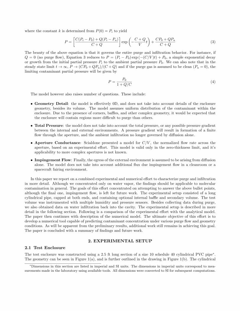
where the constant k is determined from P (0) = Pi to yield

P =

[C(Pi − P0) +Q(Pi − Pu)

C +Q

]exp

(−C +Q

Vt

)+CP0 +QPu

C +Q(3)

The beauty of the above equation is that it governs the entire purge and infiltration behavior. For instance, ifQ = 0 (no purge flow), Equation 3 reduces to P = (Pi − P0) exp (−(C/V )t) + P0, a simple exponential decayor growth from the initial partial pressure Pi to the ambient partial pressure P0. We can also note that in thesteady state limit t→∞, P → (CP0 +QPu)/(C +Q) and if the purge gas is assumed to be clean (Pu = 0), thelimiting contaminant partial pressure will be given by

P =P0

1 +Q/C(4)

The model however also raises number of questions. These include:

• Geometry Detail: the model is effectively 0D, and does not take into account details of the enclosuregeometry, besides its volume. The model assumes uniform distribution of the contaminant within theenclosure. Due to the presence of corners, baffles, and other complex geometry, it would be expected thatthe enclosure will contain regions more difficult to purge than others.

• Total Pressure: the model does not take into account the total pressure, or any possible pressure gradientbetween the internal and external environments. A pressure gradient will result in formation of a finiteflow through the aperture, and the ambient infiltration no longer governed by diffusion alone.

• Aperture Conductance: Scialdone presented a model for C/V , the normalized flow rate across theaperture, based on an experimental effort. This model is valid only in the zero-thickness limit, and it’sapplicability to more complex apertures is not known.

• Impingement Flow: Finally, the egress of the external environment is assumed to be arising from diffusionalone. The model does not take into account additional flux due impingement flow in a cleanroom or aspacecraft fairing environment.

In this paper we report on a combined experimental and numerical effort to characterize purge and infiltrationin more detail. Although we concentrated only on water vapor, the findings should be applicable to molecularcontamination in general. The goals of this effort concentrated on attempting to answer the above bullet points,although the final one, impingement flow, is left for future work. The experimental setup consisted of a longcylindrical pipe, capped at both ends, and containing optional internal baffle and secondary volume. The testvolume was instrumented with multiple humidity and pressure sensors. Besides collecting data during purge,we also obtained data on water infiltration back into the cavity. The experimental setup is described in moredetail in the following section. Following is a comparison of the experimental effort with the analytical model.The paper then continues with description of the numerical model. The ultimate objective of this effort is todevelop a numerical tool capable of predicting contaminant concentration under various purge flow and geometryconditions. As will be apparent from the preliminary results, additional work still remains in achieving this goal.The paper is concluded with a summary of findings and future work.

2. EXPERIMENTAL SETUP

2.1 Test Enclosure

The test enclosure was constructed using a 2.5 ft long section of a size 10 schedule 40 cylindrical PVC pipe∗.The geometry can be seen in Figure 1(a), and is further outlined in the drawing in Figure 1(b). The cylindrical

∗Dimensions in this section are listed in imperial and SI units. The dimensions in imperial units correspond to mea-surements made in the laboratory using available tools. All dimensions were converted to SI for subsequent computations.

configuration was selected to allow for model comparison, since we anticipated development of an azimuthally-symmetric code. Size 10 PVC end caps were fitted to both ends to seal the volume, and 3/8” diameter holeswere drilled in their centers. The depth of these holes was measured as 1.45 cm, which was slightly more thanthe typical thickness of the size 10 end cap. Due to the low inlet flow and hence low internal pressure, a frictionfit between the end caps and the pipe was deemed sufficient to seal the volume. As can be seen from Figure1(b), the length of the overlapping area was approximately 9 cm. A 1/4” AN bulkhead fitting was installed inthe inlet cap to interface with the GN2 source. An additional 3/8” diameter hole was drilled in the cylinder atthe midpoint to allow the pass-through of sensor wiring. This opening was sealed with multiple layers of Kaptontape. The volume of the test cavity was computed to be 0.0477 m3.

(a) Internal Geometry

0.1084.25[ ]

0.01270.5[ ]

0.2299[ ]

0.08893.5[ ]

0.253

9.98

[]

0.08573.375[ ]

0.01090.43[ ]

0.1264.98[ ]

0.43917.3[ ]

0.74129.2[ ]

0.02641.04[ ]

0.3915[ ]

1.02 40.13[ ]

0.1335.24[ ]

R0.17

6.71

[]

0.216 8.5[ ]

0.02220.875[ ]

0.0635

2.5

[]

0.01220.482[ ]

Sensor Pack Applicable Purge Tests Applicable Infiltration Tests

A All All

B 3, 4, 5, 6, 7, 8 3, 4, 5

C All All

D All All

E 3, 4 3

E' 5, 6 (baffle tests) 4

E'' 7, 8 (internal volume tests) 5

F All All

Units: meters [inches]

Note: Baffle only in place duringpurge tests 5 and 6, and infiltration test 4 Internal volume only in place duringpurge tests 7 and 8, and infiltration test 5

Total internal volume: 47.7 Liters

A B

E'

C D F

E

Aperture to ambient

environment

Purge gas inlet

Baffle

Internal volume

E''

(b) Test setup dimensions and sensor locations

Figure 1. Figure (a) shows a CAD drawing of the test volume. Note that the combined baffle and internal volumeconfiguration was not studied experimentally. Figure (b) shows the test dimensions and sensor locations.

The testing was performed at NASA Goddard Space Flight Center propulsion laboratory. The typical testsetup is shown in Figure 2(a). Figure 2(b) shows the inside of the test cylinder for the case containing the internalbaffle. An ultra high purity grade C gaseous nitrogen bottle source was used for most of the tests, except forthe subset utilizing internal baffle or the cup. Grade C GN2 contains at most 5.7 ppmv (parts per million byvolume) of water molecules.4 These runs were conducted using a GN2 from a dewar boil-off, due to a temporarylack of an available gas bottle. An adjustable pressure regulator was used to dial the upstream pressure to 30

psig, and an adjustable 0.1-4 scfh float-type rotameter was used to establish the inlet flow rate. 1/4” PTFE andstainless steel flex hoses and 1/4” AN fittings were used as necessary to plumb the volume to gas source.

(a) Laboratory Setup (b) Internal View with Baffle Installed

Figure 2. (a) Photograph of a typical test setup in the NASA/GSFC propulsion laboratory. (b) View of onside of the testcylinder with the baffle installed, also showing the sensor packs.

The initial set of testing was performed with no obstruction in the test volume. This setup provided thesimplest geometry, and also the closest correlation to the original Scialdone experiment. This configuration wastested at 2 scfh, 4 scfh, and 1 scfh. These flow rates approximately correspond to 1 L/min, 2 L/min, and 0.5L/min, respectively. Subsequently, the impact of internal geometry was tested. First, an internal baffle witha small central opening was included, effectively separating the cylinder into two interconnected volumes. Thebaffle was constructed from an ESD bagging material, which was taped to the cylinder wall. The volume wasalso tested with the inclusion of a secondary internal volume with a single vent facing away from the purge inlet.The secondary volume was constructed by wrapping a coffee cup in foil, and suspending it from a sensor harness.These secondary volume tests added some complexity found in an actual instrument, while being sufficientlysimple to allow correlation with the numerical analysis. All obstructed-flow testing was performed at a flow rateof 2 scfh. The tests are summarized in Table 1. At the conclusion of each test, the purge was discontinued, andthe ambient environment was allowed to infiltrate back into the cavity.

Table 1. List of purge runs and configurations

Test No. Configuration Start Date End Date Flow Rate Notes:1 Unobstructed Volume 6/11/14 6/12/14 2 scfh No temperature compensation2 Unobstructed Volume 6/13/14 6/16/14 2 scfh No temperature compensation3 Unobstructed Volume 7/1/14 7/1/14 4 scfh4 Unobstructed Volume 7/7/14 7/9/14 1 scfh5 Internal Baffle 7/9/14 7/9/14 2 scfh Flowmeter malfunction6 Internal Baffle 7/10/14 7/11/14 2 scfh7 Secondary Volume 7/17/14 7/18/14 2 scfh Loss of purge gas pressure8 Secondary Volume 7/18/14 7/21/14 2 scfh

2.2 Sensors

Sensor selection was an important part of the experimental effort. We were interested in obtaining the con-taminant concentration and pressure at multiple locations, while at the same time minimizing the impact tothe internal environment. As such, the sensors had to be both small in size, and also capable of measuringproperties of interest across the expected range of values at a fast response rate. Ease of integration with adata acquisition system was also considered. The resulting selection consisted of analog relative humidity (RH),

absolute pressure, and temperature sensors. The analog output allowed rapid prototyping and the ability toquickly and easily diagnose both hardware and software issues during the development of the test setup. Theindividual sensors are described in more detail below.

The Honeywell HIH-5030 surface mount (SMT) sensor5 was used to obtain the humidity data. This capac-itive relative humidity sensor is only approximately 1 cm long, and is capable of measuring from 0 to 100%RH. Although absolute measures would be required for eventual correlation with numerical results, the limitedavailability, high cost, and comparatively large size of absolute humidity sensors precluded this option. Absolutehumidity values must then be calculated from the relative humidity based on measured conditions (tempera-ture and pressure) in the test volume. For the purposes of this experiment, this method would be sufficientto reliably measure the moisture levels in a volume under purge. Manufacturer provided operating specifica-tions can be found in table 2. The HIH-5030 has an analog output which is ratiometric to relative humidity,Vout = Vsupply ∗ (0.00636) ∗ (RH) + 0.1515. The supply voltage (Vsupply) was 5 Vdc. Solving for RH, yieldsRH = (Vout/Vsupply−0.1515)/0.00636. The computed humidities were in a good agreement against a calibratedGE Parametrics PM880 hygrometer with a M2LR-00-010-0 probe.

Table 2. HIH-5030 Specifications

Parameter Minimum Maximum UnitAccuracy -3 +3 % RHVoltage Supply 2.7 5.5 VdcOperating Humidity 0 100 % RH

Absolute pressure was measured using the Freescale Semiconductor MPXHZ6130A sensor.6 The sensor is apiezoresistive transducer with an analog output ratiometric to absolute pressure. Manufacturer specificationscan be found in Table 3. Again, a transfer function was used to convert the sensor output voltage to pressure(in kPa), PkPa = (Vout/Vsupply + 0.07739)/0.007826.

Table 3. MPXHZ6130A Specifications

Parameter Minimum Maximum UnitAccuracy -1.5 +1.5 kPaVoltage Supply 4.75 5.25 VdcOperating Pressure 15 130 kPa

Temperature was obtained from Analog TMP36 sensor.7 Local gas temperature was needed to convert relativehumidity to absolute values. Since the experiment was conducted in a laboratory with limited control over theexternal air-conditioned environment, the temperature was seen to vary with a noticeable diurnal periodicity.Manufacturer specifications for this sensor can be found in Table 4. The measured temperature in (C) was givenby T = (Vout − 0.5) ∗ 100, where Vout is the sensor output voltage.

Table 4. TMP36 Specifications

Parameter Minimum Maximum UnitAccuracy -1.5 +1.5 ◦CVoltage Supply 2.7 5.5 VdcOperating Temperature -40 125 ◦C

2.3 Data Acquisition

National Instruments LabVIEW is often the defacto data acquisition system for collecting experimental data.However, due to the limited license availability of a LabVIEW system, an alternative was required. Initial sensorselection, testing, and calibration was performed using an Arduino micro-controller board. After success inprototyping, this platform was selected to perform the actual data collection for testing. Although this approachrequired development of the micro-controller code, the Arduino approach resulted in an increased flexibility at a

fraction of the cost of a LabVIEW system. The small size of the micro-controller board allowed the experimentto be run in multiple locations, and be moved without much effort.

In order to easily interface the sensors with the Arduino, some hardware was necessary. The selection ofsurface mount (SMT) sensors required the use of SMT to DIP boards to allow connection to the Arduino (whichuses standard 0.1” hole spacing). The humidity and pressure sensors were soldered to SOIC-14 SMT to DIPbreakout boards, and male DIP headers were attached to the SOIC-14 boards. Wiring harnesses were made toprovide power to the sensor packs, and to carry the sensor output voltages. Six sensor packs (including pressureand humidity sensors) and six wiring harnesses were assembled. A prototyping board with standard 0.1” holespacing was used to wire the sensor packs to the Arduino in parallel via the wiring harnesses. Male headersallowed this board to be attached directly to the Arduino itself, and for power, ground, and all analog voltages toreach the appropriate ports. Figures 3(a) and 3(b) show the humidity and pressure sensors surface mounted toa SOIC-14 board and the wiring to the sensor pack, and the breakout board connecting sensor pack wiring to theArduino for processing, respectively. The temperature sensors were not included in the sensor packs. Instead,one temperature sensor was suspended from a separate wire in the middle of the test volume. Another sensorwas connected by a short (about 3cm) harness to the Arduino board.

Purge flow and moisture infiltration testing was conducted using multiple sensor configurations. Initially,three sensor packs were used to measure internal conditions at a location near the purge inlet, in the middle,and at a location near the aperture. The sensors were installed near the enclosure wall, by taping the harness tothe wall using Kapton tape. One sensor pack was used outside. After two purge runs at 2 scfh and subsequenthumidity infiltration tests additional pressure and humidity sensors were added to the test volume. Locations forall setups can be found in Figure 1(b). The initial purge runs did not contain an internal temperature sensor,and used data from the external sensor for calculation of the absolute humidity.

(a) Sensor pack with wiring harness (b) Arduino Mega with breakout board

Figure 3. (a) Sensor pack containing one pressure and one humidity sensor, and (b) Arduino board used for data acquisition

2.4 Software

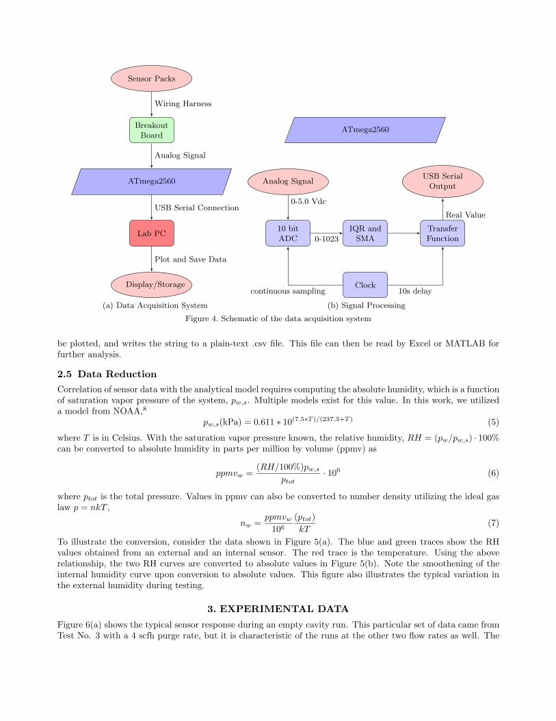
Figure 4 shows an overview of the data acquisition system and the processing performed by the Arduino. Analogvalues were constantly sampled by the Arduino micro-controller’s on-board analog to digital converter (ADC),and stored in a rolling buffer. These values were passed through a inter-quartile-range (IQR) filter in order toreject outliers. The remaining data was averaged and output over the serial communications port at a specifiedrate (every 10 seconds for this experiment).

A simple Java program was written in order to read the values transmitted by the Arduino over the serialport. This code operates separately from the Arduino, which reads and processes data whenever powered. Whenrun, the Java program receives incoming serial data as a string of values, parses this string to find values to

Sensor Packs

BreakoutBoard

ATmega2560

Lab PC

Display/Storage

Wiring Harness

Analog Signal

USB Serial Connection

Plot and Save Data

(a) Data Acquisition System

Analog Signal

10 bitADC

IQR andSMA

TransferFunction

ATmega2560

Clock

USB SerialOutput

0-5.0 Vdc

0-1023

10s delaycontinuous sampling

Real Value

(b) Signal Processing

Figure 4. Schematic of the data acquisition system

be plotted, and writes the string to a plain-text .csv file. This file can then be read by Excel or MATLAB forfurther analysis.

2.5 Data Reduction

Correlation of sensor data with the analytical model requires computing the absolute humidity, which is a functionof saturation vapor pressure of the system, pw,s. Multiple models exist for this value. In this work, we utilizeda model from NOAA,8

pw,s(kPa) = 0.611 ∗ 10(7.5∗T )/(237.3+T ) (5)

where T is in Celsius. With the saturation vapor pressure known, the relative humidity, RH = (pw/pw,s) · 100%can be converted to absolute humidity in parts per million by volume (ppmv) as

ppmvw =(RH/100%)pw,s

ptot· 106 (6)

where ptot is the total pressure. Values in ppmv can also be converted to number density utilizing the ideal gaslaw p = nkT ,

nw =ppmvw

106

(ptot)

kT(7)

To illustrate the conversion, consider the data shown in Figure 5(a). The blue and green traces show the RHvalues obtained from an external and an internal sensor. The red trace is the temperature. Using the aboverelationship, the two RH curves are converted to absolute values in Figure 5(b). Note the smoothening of theinternal humidity curve upon conversion to absolute values. This figure also illustrates the typical variation inthe external humidity during testing.

3. EXPERIMENTAL DATA

Figure 6(a) shows the typical sensor response during an empty cavity run. This particular set of data came fromTest No. 3 with a 4 scfh purge rate, but it is characteristic of the runs at the other two flow rates as well. The

0 20 40 60 80 100 1200

20

40

60

80

Time (hours)

Hu

mid

ity

(%R

H)/

Tem

per

atu

reAmbient RHInternal RH

Temperature (◦C)

(a) Raw Data

0 20 40 60 80 100 1200

0.5

1

1.5

·104

Time (hours)

Hu

mid

ity

(pp

mv)

AmbientInternal

(b) Converted Data

Figure 5. Computation of absolute humidity. Figure (a) shows relative humidity and temperature obtained from theinternal sensors. These are used to compute the absolute humidity in (b).

(a) sensor data (b) pressure and temperature

Figure 6. Experiment results for 4 scfh (∼2 L/min) flow rate purge. Note the tendency for lower humidity in the flowdirection in (a), and no impact of purge on pressure and temperature in (b).

figure plots the internal and external humidity, in parts per million. The humidity data is shown on a log scale.As can be seen from this figure, very little difference was observed between the 3 internal sensor locations (nearthe end cap containing the inlet, at the midpoint, and near the end cap containing the open aperture). Thedifference becomes apparent only once the concentration drops below 500 ppvm, corresponding roughly to 2.5%RH. It is interesting to note that the water content decreases with decreasing distance to the aperture. Thiswas unexpected, since we anticipated the highest concentration near the aperture due to water infiltration fromthe ambient environment. Likely, the finite speed of the purge gas moving through the aperture resulted in anadvective term preventing additional diffusion from the external environment.

Figure 6(b) shows the internal and external temperature and pressure for this same run. By looking at thisplot alone, it is not possible to determine when the purge flow was initiated. As such, we can note that the

(a) baffle (b) secondary volume

Figure 7. Internal humidity data for the configurations including internal obstructions: (a) baffle (run 6), (b) secondaryvolume (run 8).

purge gas does not have a significant impact on the internal temperature and pressure. The pressure drop thatforms in response to the moving fluid is too small to detect with these sensors. The slight difference between theinternal and external temperature readouts was attributed to a faulty sensor, and following this run, the secondsensor was replaced with a new unit.

The variation in internal humidity becomes more pronounced once additional objects are included in the testcavity. These results can be seen in Figure 7. The first plot shows the results for the test with the baffle. Thesecond plot shows corresponding results for the case with the secondary volume, constructed from a coffee cupwrapped in foil. Impact of the secondary volume can be seen in both sets of results. The baffle can be seen toreduce the water vapor concentration in the zone containing the purge inlet. Water concentration in this zoneis approximately 3 times smaller than in the downstream zone. In the case of the secondary volume, the waterconcentration inside the cup is approximately 7 times greater than outside. This can be attributed to the cupaperture facing away from the purge inlet. As such, it is difficult for the purge gas to enter the secondary volumeand carry away the water vapor. The removal of water vapor from within the secondary volume is then governedby diffusion arising from the the concentration gradient across the aperture. This behavior can be seen in thesimulation results presented in section 4.

3.1 Purge Model Correlation

The Scialdone model was derived assuming an empty volume, and as such, only the results from the emptycavity runs were compared against the model. Since very little variation was seen in the sensors, it made senseto average the internal sensors into a single corresponding trace. These results are plotted in Figure 8. The solidred line shows the results from the 4 scfh case, which were presented previously in Figure 6(a). The black andblue traces correspond to 2 scfh and 1 scfh, correspondingly.

The Scialdone model is governed by four sets of parameters: normalized purge flow rate Q/V , normalizedinfiltration rate C/V , the ambient partial pressure P0, and the initial partial pressure Pi. Since this modelgoverns the rate of change of some quantity, the initial and ambient concentrations in ppmv can be substitutedin lieu of the partial pressures. The Q/V parameter can also be easily computed from the known values of theflow rate Q and the enclosure empty volume V . The second parameter, C/V is not so easy to determine. Asnoted by O’Hanlon,9 in the continuum regime, volumetric flow rate through a short round tube does not have asimple analytical form. Scialdone performed a set of experiments to characterize the C value. Results from hisstudy are shown in Figure 3 in Reference 2. These results are given as a function of V/A, the volume of the testcavity divided by the aperture area. As such, it safe to assume that the given form is valid only in the limit ofthin orifices. The plot lists the relationship for the time constant τv ≡ V/C as τv = 0.42 · 24 · (V/A), where V/Cis in hours and V/A in meters. This equation is likely a typo, as the correct form should contain the exponent

Figure 8. Comparison against the analytical model. The dashed lines show the predicted water vapor decay using knownQ/V values in the Scialdone model.

Table 5. Fit parameters to experimental purge data for p = a exp(−bt) + c, t in hours

flow rate a b c2 scfh 9412.3 0.9182 270.274 scfh 10870.0 1.58895 329.151 scfh 8308.5 0.34059 600.38

of 0.25 to match the data on the log-log plot, τv = 0.42 · 24 · (V/A)0.25. Scialdone in fact alludes to this 0.25exponent in his earlier paper.1 Using the correct form of the equation, the ratio C/V can be computed as 0.0208hrs. Multiplying by volume, we obtain C = 9.95× 10−4 m−3/hr.

Using these values, the analytical model can be plotted. It is shown by the dashed line in Figure 8. As canbe seen, the agreement is only somewhat satisfactory, with a common trend existing in all three sets of curves.The analytical model predicts a must faster initial depletion of the contaminant than seen experimentally. Forinstance, at t = 120 min, the model predicted water vapor concentrations 1.5, 1.8, and 4.34 times smaller thanseen experimentally for 1, 2, and 4 scfh, respectively. The steady state value also differs between the experimentand the prediction. The sensor data indicate concentrations continuing to decay well past the time when steadystate was predicted by the model. Unfortunately, the 4 scfh run did not last long enough to obtain the steadystate value. However, by looking at the trend, it appears that both the 4 scfh and the 2 scfh cases resulted insteady state water concentrations below the predictions, while the 1 scfh run resulted in a steady concentrationhigher than predicted.

In order to study the discrepancy further, we fitted the experimental data to an equation of form p =a exp(−bt) + c. The fit coefficients are listed in Table 5 and the curves are plotted in Figure 8 with the dottedline. These fits also fail to predict the correct steady-state behavior, indicating that the response of the real systemcontains terms beyond the single exponential model. However, considering the fit parameter b = (C + Q)/Vallows us to obtain additional information about the test. Of main interest is comparing the expected purgeflow rate to characteristic value obtained from the experiment. Using the previously determined value of C, weobtain the characteristic flow rates listed in Table 6. The computed errors are well within the expected rangeof experimental error. In all three cases, it appears that the supplied purge flow rate was less than indicated bythe flow meter.

Table 6. Set and determined purge flow rates

Flow Rate Q (m3/hr) Q fit (m3/hr) Error (%)2 scfh 0.0567 0.0428 24.44 scfh 0.113 0.0748 34.01 scfh 0.0283 0.0153 46.1

(a) empty volume (b) baffle

(c) secondary volume

Figure 9. Water vapor infiltration into the cavity once the purge was stopped. The dashed line indicates the predictedresponse from the analytical model.

;

3.2 Water Infiltration

At the conclusion of each purge run, the flow was discontinued, and data collection was continued to obtain dataon water infiltration. These results are presented in Figure 9. This figure plots the water infiltration resultsfor three cases: empty cavity (corresponding to the end of Test No. 3), run with the baffle, and test with thesecondary volume. Data from all internal and external sensors is plotted. As before, the two ambient sensorsresulted in identical values. Similar trends can also be seen in the internal data, with very little variation seenin the empty cavity run. Inclusion of the internal geometry shows an impact on the sensor data. As expected,the area behind the baffle remains drier longer than the volume closer to the inlet aperture. Similarly, we cansee lower internal humidity inside the secondary volume in Figure 9(c).

The dashed line in all three plots is the predicted infiltration rate from Equation 3. A noticeable differencecan be seen in both the infiltration rate, and the steady-state behavior. The model predicts an exponentialgrowth until the internal concentration equilibrates with the ambient environment. This however was not seenexperimentally. Instead, in all infiltration cases, the internal humidity leveled off at values ranging from 50 to73% of the ambient. From Equation 2, it can be seen that independent of the value of C, P → P0 as t → ∞ ifQ = 0. This discrepancy is believed to arise to a finite concentration drop across the finite thickness aperture,

Table 7. Fit parameters to experimental infiltration data for p = a exp(−bt) + c, t in hours

case a b cempty -5983.3 -0.0628 6501.3baffle -6558.0 -0.0248 7626.6

cup -4857.8 -0.02839 5749.7

which is not taken into account in the model, which was derived assuming a zero-thickness orifice. Although notshown in the plot here, at the conclusion of each infiltration case, we removed the end cap and saw the internalsensors immediately equilibrate with the ambient reading.

We can also use these infiltration results to obtain a new estimate for C. The experimental data was fittedto an exponential of form p = a exp(−bt) + c using the online equation fitter at zunzun.com. The equation fitsare shown with a dotted line and the coefficients are listed in Table 7. Of note is the parameter b =≡ C/V .The average of these three cases is 0.03869, which is 85% larger than the 0.02086 value computed from V/C =0.42 · 24 · (V/A)0.25. The actual conductance across the aperture was higher in the experiment than expected.On the other hand, the infiltration rate decreased as the internal concentration started approaching the ambientenvironment. This finding indicates that the conductance term C is not a constant, but is instead a function ofthe concentration gradient, C = C(∇c), as well as geometry.

3.3 Sensitivity Studies

Finally, returning to Figure 8 and Equation 3, it is possible to study the sensitivity of different parameters onthe goodness of the fit. This study is presented in Figure 10 for the 2 scfh data set. The thick black line showsthe trace noted before, using the expected values for Q and C. The impact of error in the flow rate is plottedwith the dashed line. The red trace shows the deviation from the baseline if the flow rate is increased by 30%.The blue line is the counterpart to lower than expected flow rate. As can be seen, neither curve results in agood agreement, but improvement is seen for Q < Qinput. This was noted previously, and could be an indicationof flow meter calibration issues. The impact of the conductance parameter C is shown with the black dottedline. This trace shows prediction using the calculated Q, but using C obtained from the infiltration experimentdiscussed in the previous section. The impact of the purge flow impurities is shown with the thin blue line. Herewe assumed that the purge flow contains 5× the amount of water allowed for a grade C gas.

Alone, neither case results in a significant improvement. Combining the reduced flow rate and the experi-mentally determined C does however result in a notable improvement, at least for the initial decay. This plotis shown in green. The steady-state response is however incorrect, as was the case with the other cases. Thismay again be an indicator of the pressure and time dependent variation in the C term. It may also be anindicator of surface processes such as desorption and adsorption taking place. The yellow trace shows the modelprediction for comparable to the green trace, but with the constant (CP0 + QPu)/(C + Q) term multiplied byexp(−(C +Q)/V (0.06t). This double exponential form results in a much improved agreement, but the physicalmeaning of this fit still remains to be investigated. It should be pointed out that this double exponential form willresult in the internal pressure approaching zero which is a non-physical finding if any sources of the contaminantexist in the enclosure

4. NUMERICAL MODEL

In addition to the experimental effort, we also performed an initial study of the purge and infiltration behaviorusing numerical analysis. Transport of a contaminant in a moving medium is governed by the advection-diffusion(AD) equation. This equation describes the temporal evolution of concentration of some species due to threecontributions: diffusive flux, advective flux, and the production rate. Diffusive flux is governed by Fick’s law,~jdiff = −D∇c. This law describes the transport due to a concentration gradient ∇c, arising from the naturaltendency of systems to drive towards equilibrium. Advective flux governs transport due to velocity of the mediumin which the contaminant is dispersing. This term is given by ~jadv = ~vn. Inserting the two flux terms into themass conservation equation, ∂c/∂t+∇ ·~j = R, yields the advection-diffusion equation,

∂c

∂t+∇ · (−D∇c+ ~uc) = R (8)

Figure 10. Impact of various parameters on the correlation of the Scialdone model with experimental data. The doubleexponential curve plots a hypothetical model in which the constant (CP0 +QPu)/(C +Q) terms decays as an exponentialof time.

where c is concentration of the contaminant. In this work, the concentration was set to the number densityn, given in units of number of molecules per m3. The source term R governs a volumetric mass creation (forinstance due to a chemical reaction), and was set to zero in the simulation. Instead, the ambient environmentwas introduced through the boundary conditions. The binary diffusion coefficient D was set to 0.256× 104 m2/sper Ref. 10.

Computing the advective flux requires information on the velocity of the medium. In the case of the purgeflow, this is the nitrogen gas velocity, and it can be calculated from the Navier-Stokes (NS) equations. Since theflow speed (u = Q/A) was highly subsonic, the incompressible form of the NS equations can be utilized. It isgiven by

∂~u

∂t+ ~u∇ · ~u = −1

ρ∇p+

µ

ρ

(∇2~u

)(9)

From the saturation vapor pressure equation 5, it can be seen that the water forms only about 1% of the totalatmospheric pressure. As such, it is safe to assume that the purge flow will not be affected by the concentrationof the water vapor. This then allows us to decouple Equation 9 from Equation 8. The solution can be obtainedby first using the Navier-Stokes equation to march the velocity field forward, then using the newly computedvelocity to update the water concentration, and finally repeating the process until the specified amount of realtime is simulated. In order to speed up the calculation, the simulation was performed on a two-dimensionalazimuthally-symmetric (RZ) domain. The following paragraphs describe details of the two solvers, and alsopresent the preliminary simulation results. The code was developed in Java. Subset of the cases was executed onthe Amazon Web Services Elastic Compute Cloud (AWS EC2), with the rest executed on a desktop workstation.For the case of infiltration (with no purge flowing), the code was able to compute a weeks worth of results inabout a day.

4.1 Advection-Diffusion Solver

Both the AD and NS equations were solved using the Finite Volume Method (FVM) with a staggered grid.This approach is particularly suitable to this problem since it easily allows setting of zero-flux condition on solidwalls. In the FVM approach, the computational domain is divided into cells (control volumes). Quantities ofinterest are assumed to be known at cell centers. Fluxes and velocities are known along cell edges, resulting in astaggered grid. Discretization equations are computed by rewriting the governing equation using the divergencetheorem to obtain surface integrals. To illustrate this method, let’s consider the AD equation 8. We take volume

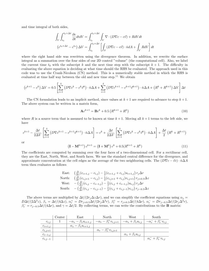
and time integral of both sides,∫V

∫ t0+∆t

t0

∂c

∂tdtdV =

∫ t0+∆t

t0

∫V

∇ · (D∇c− c~v) +RdV dt

(ct0+∆t − ct0

)∆V =

∫ t0+∆t

t0

[∫S

(D∇c− c~v) · ndA+

∫V

RdV

]dt

where the right hand side was rewritten using the divergence theorem. In addition, we rewrite the surfaceintegral as a summation over the four sides of our 2D control ”volume” (the computational cell). Also, we labelthe current time t0 with the subscript k and the next time step with the subscript k + 1. The difficulty inevaluating the above equation is deciding at what time should the RHS be evaluated. The approach used in thiscode was to use the Crank-Nicolson (CN) method. This is a numerically stable method in which the RHS isevaluated at time half way between the old and new time step.11 We obtain

(ck+1 − ck

)∆V = 0.5

[4∑

i=1

(D∇ck − ck~vk

)· n∆A+

4∑i=1

(D∇ck+1 − ck+1~vk+1

)· n∆A+

(Rk +Rk+1

)∆V

]∆t

The CN formulation leads to an implicit method, since values at k+ 1 are required to advance to step k+ 1.The above system can be written in a matrix form,

Ack+1 = Bck + 0.5(Rk+1 +Rk

)(10)

where R is a source term that is assumed to be known at time k+ 1. Moving all k+ 1 terms to the left side, wehave

ck+1 − ∆t

2∆V

[4∑

i=1

(D∇ck+1 − ck+1~vk+1

)· n∆A

]= ck +

∆t

2∆V

[4∑

i=1

(D∇ck − ck~vk

)· n∆A

]+

∆t

2

(Rk +Rk+1

)or (

I−Mk+1)ck+1 =

(I + Mk

)ck + 0.5(Rk+1 +Rk) (11)

The coefficients are computed by summing over the four faces of a two-dimensional cell. For a rectilinear cell,they are the East, North, West, and South faces. We use the standard central difference for the divergence, andapproximate concentration at the cell edges as the average of the two neighboring cells. The (D∇c− ~vc) · n∆Aterm then evaluates as follows

East:(

D∆z (ci+1,j − ci,j)− 1

2 (ci+1,j + ci,j)ui+1,j

)rj∆r

North:(

D∆r (ci,j+1 − ci,j)− 1

2 (ci,j+1 + ci,j)vi,j+1

)rj+0.5∆z

West: −(

D∆z (ci,j − ci−1,j)− 1

2 (ci,j + ci−1,j)ui,j)rj∆r

South: −(

D∆r (ci,j − ci,j−1)− 1

2 (ci,j + ci,j−1)vi,j)rj−0.5∆z

The above terms are multiplied by ∆t/(2rj∆z∆r), and we can simplify the coefficient equations using αz =D∆t/(2∆2z), βz = ∆t/(4∆z), α+

r = Drj+0.5∆t/(2rj∆2r), β+

r = rj+0.5∆t/(4∆r), α−r = Drj−0.5∆t/(2rj∆

2r),β−r = rj−0.5∆t/(4∆r), and γ = ∆t/2. By collecting terms, we can write the contributions to the B matrix:

Center East North West Southci,j 1 −αz − βzui+1,j −αr − β+

r vi,j+1 −αz + βzui,j −α−r + β−

r vi,jci+1,j αz − βzui+1,j

ci,j+1 αr − β+r vi,j+1

ci−1,j αz + βzui,jci,j−1 α−

r + β−r vi,j

and similarly for the A matrix (note, velocities here are at the k + 1 time):

Center East North West Southci,j 1 αz + βzui+1,j αr + β+

r vi,j+1 αz − βzui,j α−r − β−

r vi,jci+1,j −αz + βzui+1,j

ci,j+1 −αr + β+r vi,j+1

ci−1,j −αz − βzui,jci,j−1 −α−

r − β−r vi,j

4.2 Boundary Conditions and Geometry

There are two types of boundary conditions applicable to the advection-diffusion equation: specified concentra-tion, and specified normal flux. The specified concentration simply prescribes the value of c along the Dirichlet

boundary, c = g(s) ∈ ΓD. The specified flux boundary is derived as(~jadv +~jdiff

)· n ≡ (c~v−D∇c) · n = h(s) ∈

ΓR. Specifically for the zero flux boundary, we have (c~v −D∇C) · n = 0. Specifying this boundary condition inthe finite volume method is easy - the terms are simply not included for the zero-flux faces.

The zero-flux boundary was applied along all solid walls. The geometry of the problem was set from in-formation presented in the drawing in Figure 1(b) by ”sugar cubing” the internal cells. The location of eachcell’s centroid was computed, and if the location was outside the fluid domain, the entire cell was marked assolid. Outside the tube, the computational domain contained a section representing the ambient environment.The outer z and r edges of this ambient zone were set to a time-varying Dirichlet condition, with concentrationvarying according to the experimentally-collected ambient humidity data, e.g. the blue curve in Figure 5(b).The zero flux boundary was also applied along the axis of symmetry, (~j · er)r=0 = 0.

4.3 Infiltration Results

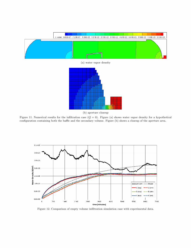
Figure 11(a) shows a snapshot of the computed water vapor density for a hypothetical case containing both thebaffle and the secondary volume. This figure is meant to illustrate the variation in the internal contaminantconcentration once a complex internal geometry is considered. The baffle is seen to have a noticeable affect onreducing the infiltration rate to the region located behind the baffle. Variation can also be seen between thewater vapor concentration inside the secondary volume, however, at the particular time of this snapshot, theinternal concentration is becoming comparable to that of the surrounding cavity.

This figure also illustrates the small external region corresponding to the ambient environment. A closeup ofthis region is shown in Figure 11(b). This figure plots the cell-centered concentration values and also illustrates the”sugar-cubing” of the geometry. Of importance is the concentration gradient that develops across the aperture.This is an artifact of a finite-thickness aperture, and is believed to be the reason for the internal concentrationnot reaching the ambient humidity, even after a prolonged infiltration test.

In addition to being able to obtain the graphical representation of the two-dimensional variation in thecontaminant concentration, the simulation code was also instrumented with virtual sensors that collected localpressure and humidity as a function of time. The location of these sensors was selected according to theexperimental sensor placement. The comparison between the numerical and experimental data can be seen inFigure 4.3. This figure plots results for an empty cavity case, in which neither the baffle nor the cup were present.The black line is the ambient humidity which was used to set the ambient Dirichlet boundary condition. Ascan be seen, the numerical predictions are in line with the experiment, however, a noticeable discrepancy exists.The simulation seems to predict a similar asymptoting behavior, however the rate of infiltration increase differsfrom data. Specifically, the experiment resulted in a faster initial build up of the water vapor, followed by arapid decay in rate. The simulation on the other hand resulted in a much more linear response. The spatialdifference in sensor data was also greater for the numerical case. These discrepancies will be investigated as partof future work. One possible explanation is that the experimental case includes additional sources of water, suchas surface desorption, that are not included in the experiment.

(a) water vapor density

(b) aperture closeup

Figure 11. Numerical results for the infiltration case (Q = 0). Figure (a) shows water vapor density for a hypotheticalconfiguration containing both the baffle and the secondary volume. Figure (b) shows a closeup of the aperture area.

Figure 12. Comparison of empty volume infiltration simulation case with experimental data.

4.4 Navier-Stokes Solver

The incompressible Navier-Stokes equation 9 is solved using the projection method.12 In this method, thevelocity update is split into two parts: a part due to advection and viscous diffusion, and a part due to thepressure gradient. First, a temporary velocity is computed,

~ut − ~uk

∆t= −~uk∇ · ~uk + ν

(∇2~uk

)(12)

Then, the pressure gradient is added to obtain the velocity at the next time step,

~uk+1 − ~ut

∆t= −1

ρ∇p (13)

Since from mass conservation ∇ · ~uk+1 = 0, we can write

∆t

ρ∇2p = ∇ · ~ut (14)

This Poisson’s equation is solved using the preconditioned conjugate gradient (PCG) solver, which is also usedin the implicit AD code. The resulting pressure field is then used in Equation 13 to compute the new velocityfield.

The NS solver also utilizes a staggered grid with pressure known at the cell center, and velocities known atthe midpoint of the cell edges. The boundary conditions for the solver included zero velocity along walls (no-slipcondition) and no flow across the axis of symmetry. A well-developed flow ∂u/∂r = 0 was specified at the outflowboundary. The purge flow was specified by setting u = uinlet along cell edges corresponding to the purge inlet.

4.5 Preliminary Purge Flow Results

Unlike the AD code, the NS solver utilized an explicit time integration scheme, and as such required smallertime steps than allowed under the implicit scheme. Yet even with smaller time steps that satisfied the CFLcondition, the combined AD+NS approach was found to result in regions with negative density. This finding islikely indicative in a remaining bug in the solver that will be investigated as part of future work. The resultspresented in this section were computed using a density limiter n > 1e19m−3. Presence of such a limiter howeverresults in an artificial mass increase, since contaminant concentration is numerically increased if it falls belowthe threshold value.

The preliminary purge flow simulation results are shown in Figure 13(a). This figure plots the water vaporconcentration for the hypothetical case containing both the baffle and the cup, with the initial internal concen-tration equal to the ambient environment, and purge flow rate Q = 1L/min. Figure 13(b) shows the flow speedat the corresponding time. As expected, the flow speed is increased whenever the flow encounters an obstruction,such as the baffle opening or the exit aperture. We can also note from these plots the impact of advection onthe contaminant concentration. In regions with increased flow velocity (such as through the aperture), there isa significant decrease in water vapor concentration compared to the surrounding environment. This is anotheraspect that is not included in the analytical model of Scialdone, but is discussed in the work of Woronowicz.However, diffusion does play an important role in the contaminant transfer. This is mainly visible in the sec-ondary volume. The primary flow passes over the cup, and ends up reducing the water concentration in frontof the cup opening. The resulting concentration gradient then helps drive off the internal moisture from withinthis secondary volume.

Fluid flows can be described as laminar or turbulent, with the Reynolds number providing an indicator ofthe expected flow regime. For a flow in a pipe, the Reynolds number is given by Re = uD/ν, where u is the flowspeed, D is the pipe diameter, and ν = µ/ρ is the kinematic viscosity. Generally, pipe flow with Re < 2300 isconsidered to be laminar, and turbulent for Re > 4000. Using the test pipe and aperture diameters of 0.25 and0.01 m, respectively, we can compute the two Reynolds number to be Repipe = 3630 and Reaperture = 160. In theprevious calculation, flow speed was computed as u ≡ Q/A = 0.21m/s for Q = 1L/min, and ν = 1.46×10−5m2/s.This is in fact confirmed by the numerical simulation. A laminar flow can be seen to exist across the aperture

(a) water vapor density

(b) flow speed

Figure 13. Preliminary purge flow simulation results. Figure (a) shows the water vapor density while (b) shows the flowspeed.

and the baffle opening. However, within the cavity, several vortexes can be seen to form. This vortex formationresults in some regions of the cavity being more difficult to dry off than other. The vortex formation mayhowever be assisted by the inlet boundary condition, containing only an axial flow. As such, the solution doeshave some resemblance to the lid-driven cavity case often studied in fluid-dynamics. It should also be noted thatthe preliminary results discussed in this section were computed without including treatment for turbulent flowin the numerical code. Turbulent features can be studied using approaches such as RANS, in which the flow issplit into a time-averaged value, and a random turbulent oscillation. Inclusion of the RANS model and studyingthe impact of the inlet boundary condition is left for future work.

5. CONCLUSION AND FUTURE WORK

In this paper we summarized an experimental and numerical effort to study the removal and infiltration of acontaminant such as water vapor into an enclosed cavity. More specifically, the results were compared againsta well known analytical model of Scialdone. By purging a cylindrical cavity containing multiple internal sen-sors, we found that although some similarities exist between the experiment and the model, there were alsoseveral discrepancies. The primary differences existed in the rate of contaminant removal and in the steadystate behavior. The analytical model predicted a faster initial dry off, but higher steady state contaminantconcentration. Some of these findings can be attributed to the fact that the model is based on the assumptionof the ambient contaminant diffusing into the cavity, without taking into account impact of flow velocity. Byallowing the external humidity to diffuse into the cavity once the purge was stopped, we were also obtain data ona contaminant infiltration. The most interesting finding here was that the internal concentration never reachedthe ambient levels, but instead leveled off at values ranging from 50 to 73% of the ambient. This finding seemsto indicate that the ”conductance” through the aperture is not a constant value but is instead a function of theconcentration gradient.

Besides providing data for the comparison with the analytical model, the experiment was also used to obtaina set of validation data for a numerical simulation. The numerical effort was based on a combined advection-diffusion and incompressible Navier-Stokes solver. Results from the simulation were presented but additionalwork still remains in improving the agreement. Once better agreement is achieved, we anticipate using the toolto study the purge and infiltration problem in more detail. Specifically, we will be interested in determiningthe temporal variation in the aperture conductance, and also will use the code to study the impact of externalimpingement flow on the infiltration rate. By combining the code with a particle tracing algorithm13 we willalso be able to study the impact of purge on particulate contamination, including in a complex flow field suchas a spacecraft fairing.14

Acknowledgement

The authors would like to acknowledge Gregory Bennett (GOES-R engineering co-op) for performing initialresearch on pressure and humidity sensors; John Fiorello Jr. and Zoe Dormuth (GOES-R engineering interns)for supporting data collection activities; Steve McKim, Hal Baesh, and the rest of GSFC propulsion lab formaking the testing possible; and Rob Studer at GOES-R, and Mark Secunda, David Hughes, Mike Woronowiczand Evelyn Lambert at NASA/GSFC contamination branch for fruitful discussions on purge testing and analysis.This effort was supported by the GOES-R and MMS projects.

REFERENCES

[1] Scialdone, J. J., “Water-vapor pressure control in a volume,” in [NASA Technical Paper 1172 ], (1978).

[2] Scialdone, J. J., “Preventing molecular and particulate infiltration in a confined volume,” in [SPIE Confer-ence on Optical System Contamination ], 3784 (1999).

[3] Woronowicz, M., “Observations on one-dimensional counterflow diffusion problem,” in [SPIE Conference onOptical System Contamination ], (2002).

[4] Author, U., “Preformance specification: propellant pressurizing agent, nitrogen,” Tech. Rep. MIL-PRF-27401D (1995).

[5] “Low voltage humidity sensors.” http://sensing.honeywell.com/honeywell-sensing-hih5030-5031%

20series-product-sheet-009050-2-en.pdf?name=HIH-5030-001.

[6] “Media resistant and high temperature accuracy integrated silicon pressure sensor for measuring absolutepressure.” http://cache.freescale.com/files/sensors/doc/data_sheet/MPXHZ6130A.pdf.

[7] “Low voltage temperature sensors.” http://www.analog.com/static/imported-files/data_sheets/

TMP35_36_37.pdf.

[8] “Vapor pressure.” http://www.srh.noaa.gov/images/epz/wxcalc/vaporPressure.pdf.

[9] O’Hanlon, J. F., [A user’s guide to vacuum technology ], John Wiley & Sons (2005).

[10] Schwertz, F. and Brow, J. E., “Diffusivity of water vapor in some common gases,” The Journal of ChemicalPhysics 19(5), 640–646 (1951).

[11] Tanehill, J., Anderson, D. A., and Pletcher, R. H., “Computational fluid mechanics and heat transfer,”Taylor &Francis (1997).

[12] Chorin, A. J., “On the convergence of discrete approximations to the navier-stokes equations,” Mathematicsof Computation 23(106), 341–353 (1969).

[13] Brieda, L., Gordon, T., and Arun, S., “Analysis of molecular conductance through a labyrinth vent,” in[SPIE Optics and Photonics ], (2014).

[14] Brieda, L., Barrie, A., Hughes, D., and Errigo, T., “Analysis of particulate contamination during launch ofthe mms mission,” in [SPIE Optics and Photonics ], (2010).