Diagnosing and Mitigating Market Power in Chile’sElectricity Industry.∗

M.Soledad Arellano†

Universidad de Chile

May 12, 2003

Abstract

This paper examines the incentives to exercise market power that generators wouldface and the different strategies that they would follow if all electricity supplies in Chilewere traded in an hourly-unregulated spot market. The industry is modeled as a Cournotduopoly with a competitive fringe; particular care is given to the hydro schedulingdecision. Quantitative simulations of the strategic behavior of generators indicate thatthe largest generator (”Endesa”) would have the incentive and ability to exercise marketpower unilaterally. It would do so by scheduling its hydro resources, which are shown tobe the real source of its market power, in order to take advantage of differences in priceelasticity: too little supply to high demand periods and too much to low demand periods.The following market power mitigation measures are also analyzed: (a) requiring Endesato divest some of its generating capacity to create more competitors and (b) requiringthe dominant generators to enter into fixed price forward contracts for power coveringa large share of their generating capacity. Splitting the largest producer in two or moresmaller firms turns the market equilibrium closer to the competitive equilibrium asdivested plants are more intensely used. Contracting practices proved to be an effectivetool to prevent large producers from exercising market power in the spot market. Inaddition, a more efficient hydro scheduling resulted. Conditions for the development ofa voluntary contract market are analyzed, as it is not practical to rely permanently onvesting contracts imposed for the transition period.

JEL Codes: D43, L11, L13, L94Key Words: Electric Utilities; Market Power; Scheduling of Hydro-Reservoirs; Contracts;Chile’s Electricity Industry

∗I am grateful to Paul Joskow and Franklin Fisher for their comments and suggestions. I also benefited fromcomments made by participants at the IO lunches and the IO Seminar held at MIT and from Seminars heldat the Instituto de Economia, Universidad Católica de Chile and Centro de Economía Aplicada, Universidadde Chile. Financial support from the MIT Center for Energy and Environmental Policy Research (CEEPR)is gratefully acknowledged.

†Center of Applied Economics, Department of Industrial Engeneering, Universidad de Chile. República701, Santiago Chile. Email: sarellano@dii.uchile.cl

1

1 IntroductionChile reformed and restructured its power industry in the early 1980’s. Competition amonggenerators was promoted and a ’simulated’ spot market was created. Prices in this marketwere not truly deregulated (except for the largest consumers who chose to enter into contractsdirectly with generators) but were based in the short-run marginal costs of generators in thesystem and the associated least cost dispatch. Two decades later, policymakers in Chile arediscussing the desirability of further de-regulating Chile’s wholesale electricity market. Inparticular, the simulated spot market that is in place today would be replaced by a real un-regulated spot market in which generators would be free to bid whatever prices they choosewith competition between generators determining the bids and market clearing prices. Onemajor concern that has been raised regarding this spot market deregulation proposal is thatthe high degree of concentration in the generation segment would enable incumbent gener-ators to exercise market power, leading to prices far above competitive levels. Internationalexperience on restructuring and reforms of the electricity industry on different countries (UK,US, New Zealand and so on) has taught us that this concern is legitimate. First of all, poli-cymakers must realize that the electricity industry is prone to the exercise of market power,as electricity cannot be stored, demand is very inelastic, producers interact very frequently,capacity constraints may be binding when demand is high and thus even a small supplier maybe able to profitably and unilaterally increase the market price by withholding supplies fromthe market. The importance of an adequate number of generating companies that competein the wholesale market has also been emphasized. For instance, the experience in the UK,has shed light on the market power problems that high concentration may create and dur-ing the late 1990s, the government embarked on a program to reduce concentration throughdivestiture and the encouragement of competitive entry. 1

This paper examines the incentives to exercise market power that generators would faceand the different strategies that they would follow if all electricity supplies in Chile were tradedin an hourly-unregulated spot market. The analysis will focus on the impact of such a reformin the biggest Chilean electric system, called the ”SIC”. Its installed capacity amounts to 6660MW. Electricity is produced by 20 different generating companies but two economic groups(called Endesa and Gener) control 76% of total installed capacity and 71% of total generation.These firms differ in size, composition of its production portfolio and associated marginal costfunctions. Endesa (”Firm 1”) owns a mixed hydro/thermal portfolio, concentrates 78% ofthe systems’ hydro reservoir capacity and its thermal capacity covers a wide range of fuel andefficiency levels. Gener (”Firm 2”) is basically a purely thermal producer and concentrates thelargest fraction of thermal resources in the SIC (46%). Analyzing Chile’s sector is especiallyinteresting because a large fraction of its generating capacity is stored hydro. Previousanalyses have focused on systems that were either mostly thermal or entirely hydro (e.g.Norway).Following Borenstein and Bushnell (1999) and Bushnell (1998), Chile’s electricity market

is modeled as a Cournot duopoly with a competitive fringe. Particular care is given to themodeling of hydro resources, which are not only important because of its large share in totalinstalled capacity and in total generation (61% and 62% respectively in 2000), but becauseof its impact on the incentives faced by producers when competing. As it will be analyzed in

1For more details on the lessons learned from the UK and US experience, see Joskow (2002).

2

the paper, having hydro resources as a source of electric generation, means that firms do nottake static production decisions at each moment in time, but that firms have to take accountthat more water used today, means less water is available for tomorrow: the model becomesdynamic rather than static.Quantitative simulation results suggest that if an unregulated spot market were imple-

mented in Chile, prices could rise far above competitive levels as suppliers, in particularEndesa, the largest supplier, would exercise unilateral market power. The large thermalportfolio owned by Gener, the second largest generator, is not enough for the exercise of mar-ket power, as the relevant plants are mostly base load plants. Indeed, Endesa has so muchmarket power and can move prices up so much, that Gener’s optimal strategy is to produce atfull capacity, profiting from the high prices set by Endesa. Even though Endesa keeps mostof its thermal plants outside of the market, the real source of its market power is its largehydro capacity. In particular, it schedules its hydro production in order to exploit differencesin price elasticity, allocating too little supply to high demand periods and too much to lowdemand periods, relative to the competitive equilibrium. This hydro scheduling strategy maybe observed no matter what planning horizon is assumed in the model (a month, a year);the only ”requirement” is that there is enough ”inter-period” differences in demand elastic-ity. The smaller are the intertemporal differences in demand elasticities, the closer is thehydro scheduling strategy to the traditional competitive supply-demand or value-maximizingoptimization analysis’ conclusions (i.e. water is stored when it is relatively abundant andreleased when it is relatively scarce). The importance of hydro resources for Endesa is suchthat when hydro flows are reduced (as occurs if the hydrological year is ”dry”), Endesa losesits market power. Under these circumstances, Gener has incentives to act strategically toincrease prices, but the resulting prices are still lower than when Endesa had all of its capacityunder normal hydrological conditions. Not surprisingly, alternative assumptions about theelasticity of demand for electricity turned out to be very important, as the more elastic isdemand, the less market power can be exercised.These results suggest that the exercise of market power should be of considerable con-

cern in Chile and that mitigation measures will be needed to prevent market power abusesin the newly deregulated spot market. Different market rules have been implemented as ashield against market power abuses throughout the world. Regulators have relied on elementssuch as splitting the generating companies into many small firms in order to reduce the de-gree of concentration of the generation sector (Australia, Argentina), vesting contracts inorder to reduce generating companies’ incentives to charge high prices (England and Wales,Australia) and continuing regulatory surveillance and threats (England and Wales, UnitedStates), among others. Each country / electric power system is different in terms of marketstructure, size, mix of generating technology and even culture. As a consequence, the experi-ence of another market, even if successful, should not blindly be put into practice elsewherewithout first carefully analyzing the individual characteristics of the specific electric powerindustry subject to reform. The effect of different market power mitigation measures thathave been implemented in other restructured electricity markets are also thoroughly analyzedin this paper for the case of Chile’s electricity industry. In particular, I analyze and estimatethe impact of two different sets of measures that could be implemented to reduce the incen-tive and ability of the dominant firms to exercise market power in a spot wholesale electricitymarket in Chile: (a) requiring the largest firm to divest some of its generating assets and (b)requiring the largest firms to enter into fixed price forward contracts covering a large share

3

of their capacity. I compare the new market equilibrium to the competitive equilibrium andto the base model equilibrium, in terms of aggregate levels, allocation of resources, markupsand overall welfare (when possible).The divestiture of some of Firm 1’s generating assets, either thermal or hydro storage

plants, turns the market equilibrium closer to the competitive equilibrium not only in termsof levels (prices and output) but also in terms of the allocation of resources, as former Firm1’s plants are more intensely and efficiently used and this more than compensates for anyreduction in production by the remaining producers with unilateral market power. Theapplication of fixed price forward contracts proved to be an effective tool to prevent largeproducers from exercising market power in the spot market. In addition, a more efficienthydro scheduling resulted. It is argued that it is not practical to rely permanently on vestingcontracts to ensure the development of the contract market as these contracts will eventuallyexpire and if conditions are not given for an appropriate voluntary contracting, market powerabusive practices will certainly take place at that time. It is emphasized that the regulationof the industry as a whole (as opposed to the contract market) must provide the incentivesfor producers and consumers to contract.This paper is organized as follows: the next chapter reviews the main findings of the

literature that are related to the topics covered in the paper. In Chapter 3 I briefly describethe Chilean power industry. In the fourth Chapter I analyze the model that will be the basictool for the analysis of market power in Chile’s electricity industry. Data used to estimate themodel are reported in Chapter 5. Quantitative simulations of each generators’ strategy andthe resulting market equilibrium are estimated under different assumptions in Chapter 6. InChapter 7, a modified version of the basic model is used to estimate the impact of two setsof mitigation measures. Both a qualitative and a quantitative analysis are done. Chapter 8concludes.

2 Literature ReviewThis paper is related to three areas of research: the modeling of electricity markets in orderto (ex-ante) simulate strategic behavior after the industry has been deregulated, the analysisof the strategic use of hydro resources to exercise market power and the impact of forwardcontracting on the incentives producers face to exercise market power.Three types of model have been used to simulate the strategic behavior of electricity firms.

In the supply function equilibrium (SFE) approach, used by Green and Newbery (1992) andHalseth (1998) based on the work by Klemperer and Meyer (1989), the producers bid a supplyfunction that relates quantity supplied to the market price. In the general case, the duopolysupply lies between the competitive and Cournot equilibrium; the range of feasible equilibriais reduced when uncertainty is added to the model.Green and Newbery (1992) modeled the England and Wales electricity market using the

Supply Function Equilibrium (SFE) framework developed by Klemperer and Meyer (1989)as applied to an empirical characterization of supply and demand, designed to match theattributes of the electricity system in England and Wales (making alternative assumptionsabout the elasticity of demand).2 They first present simulated values for prices, output

2Von der Fehr and Harbord (1993) and Halseth (1998) criticize on theoretical grounds the Green andNewbery (1992) use of the SFE approach.

4

and welfare for the duopoly case. They found that generators were able to drive prices farabove competitive levels, depending on the assumed elasticity of demand, while creating asignificant deadweight loss and producing supra-competitive profits for the generators.3 Theythen examined the impact of restructuring the industry so that there were five equal-sizedfirms. In this case, the equilibrium price was significantly lower and close to competitivelevels. In order to take account of the effect of potential entry, they examined the effectsof entry in the duopoly case under alternative assumptions about the price responses of theincumbents to the entry of generators who acted as price takers. If the incumbents adopteda strategy of not responding to entry by lowering prices, substantial entry was attracted bythe excess profits in the system. Eventually entry eroded the incumbents’ profits completely,yielding an equilibrium with inefficient expenditures on new generating capacity and highprices. The welfare losses in these cases were very large.Halseth (1998) used the SFE approach to analyze the potential for market power in the

Nordic market. In his model, the supply function is restricted to be linear, with a constantmarkup over marginal cost. This markup is independent of the particular technology usedby the producer but it varies between the different time periods. Asymmetry in productiontechnologies is incorporated through the marginal cost function (each production level is as-sociated to a specific marginal technology (hydro, nuclear or thermal). Due to the importanceof hydro production in the Nordic market (it accounts for 50% of annual production), thehydro scheduling issue is explicitly modeled. In particular, annual hydro production is re-stricted to be less than the annual inflow and the water inflow that is stored between periodshas to be within the reservoir capacity. He found that the potential for market power was lessthan expected due to the fringe’s excess capacity. Only two of the six largest producers hadincentives to reduce production.4 Remaining producers did not have incentive to do so. Inparticular, he found that hydro producers were not interested in reducing its market supply.He argued that since all of its income came from hydro production (with a very low marginalcost), the price increase had to be very large in order to induce it not to use its generatingcapacity to the full.5 It should be noted that all the results of this model are reported inannual terms. In particular, he found that hydro generating capacity was used to the full inthe year. However, nothing is said regarding how it is allocated throughout the year. Thisis an important omission because it may be the case that hydro producers do not exercisemarket power by using less than its hydro capacity but through a strategy that distinguishesbetween periods of high demand from periods of low demand.Auction theory has also been used to analyze strategic behavior in the electricity market.

Von der Fehr and Harbord (1993) model the UK electricity spot market as a first price, sealed-bid, multiple unit private-value auction with a random number of units. In their model,generators simultaneously bid supply schedules (reflecting different prices for each individualplant), then demand is realized and the market price is given by the offer price of the marginalplant. They argue that producers face two opposing forces when bidding: by bidding ahigh price, the producer gets higher revenue but a lower probability of being dispatched.

3Wolfram (1999) found that prices in the British market had been much lower than what Green andNewbery (1992) predicted.

4These two producers are Vattenfall and IVO. The portfolio of the first one is split between hydro (42%),nuclear (48%) and conventional thermal plants (10%). IVO is mostly a thermal producer.

5 Johnsen et al (1999) concluded from this result that market power cannot be exercised in a marketdominated by hydroelectric producers, to what they add, unless transmission constraint binds.

5

Equilibrium has different properties depending on the demand level. In particular, whendemand is low, producers bid a price equal to the marginal cost of the least efficient generatorand equilibrium is unique. When demand is high, there are multiple equilibria and the priceis equal to the highest admissible price.6 They remark that some of these equilibria mayresult in inefficient dispatching: the high cost generator will be dispatched with its totalcapacity if it submitted the lowest bid, while the low cost generator will be dispatched foronly a fraction of it. Finally they argue that their model is supported by the bidding behaviorobserved in the UK electricity industry from May 1990 to April 1991. In particular, theyreport that while bids were close to generation cost at the beginning of the period, theydiverged thereafter, Even though contracts were in place in the first part of the analyzedperiod, they argue that contracting practice is not a plausible explanation to the observedbidding behavior because contracts started to expire after the change of pattern took place.The coincidence of the first period with the low demand season (warm weather) and thesecond with the high demand season (cold weather) makes their model a more appropriateexplanation. It should be noticed however that they analyzed a very short period. In orderto be really able to separate the contract effect from the high/low demand effect, and in thisway to get more conclusive support to their theory, the following seasons should be analyzed.7

Finally a third approach that has been used in the literature is to model the electricityindustry as a Cournot oligopoly where producers are assumed to bid fix quantities. An-dersson and Bergman (1995) simulated market behavior of the Swedish electricity industryafter deregulation took place. They assumed a constant elasticity demand function (with anelasticity of demand equal to 0.3 in the main case), constant marginal costs for hydro andnuclear power plants and a non-linear marginal cost function for conventional thermal units.They found that prices would increase and production would be constrained. In particular,they found that the Cournot price equilibrium was 36% higher than the current (base) caseand 62% than the Bertrand equilibrium. Markups were not analyzed. They also analyzedthe impact of alternative market structures like splitting the largest company in 2 firms ofthe same size and a merge between the six smallest companies. In both cases equilibriumprice was reduced below the base case. Finally they analyzed the impact of increased priceresponsiveness solving the model for a higher elasticity value (0.6). Since hydro production ismodeled on an average basis, nothing is said regarding how resources are allocated within theyear (for instance there is no differentiation between peak and off peak periods). In addition,nothing is said regarding how the portfolio of resources is used and how it compares to thebase and Bertrand equilibrium cases. This is an important omission given the importance ofhydro resources in the Swedish electricity market.Borenstein and Bushnell (1999) and Bushnell (1998) modeled the California power in-

dustry as a Cournot triopoly with a competitive fringe.8 Cournot producers face a residualdemand where must run generation, the fringe’s supply and hydro generation in the case ofBorenstein and Bushnell (1999) are subtracted from total demand. Marginal cost functionswere estimated using cost data at the plant level. A big difference between those articles isgiven by the treatment of hydro resources: Bushnell (1998) assumes that Cournot producers

6Multiplicity of equilibria is given by the fact that both producers want to be the ”low bidder” becausethe received price is the same but the producer is ranked first, and thus output is greater.

7Wolfram (1998) analyzes the bidding behavior in the UK and tests the theoretical predictions of the multiunit auction theory.

8Their market definitions are slightly different.

6

use them strategically while Borenstein and Bushnell (1999) assume that they are allocatedcompetitively.9 In other words, in Bushnell (1998)’s model, hydro producers are ”allowed”to store water inflows from one period and use them in another one in order to manipulateprices. As a result, in his model the different periods are not independent and thus themaximization has to be solved simultaneously over the entire planning horizon, as opposedto Borenstein and Bushnell (1999)’s model where each period can be treated independently.Borenstein and Bushnell (1999) use a constant elasticity demand and estimate the model fora range of demand elasticity values (-0.1, -0.4 and -1.0) and six different demand levels. Theyfound that the potential for market power was greater when demand was high and the fringe’scapacity was exhausted, making it impossible for the small producers to increase production.In lower demand hours, Cournot producers had less incentive to withhold production becausethe fringe had excess capacity. In addition they found that the more elastic was demand, theless was the incentive to exercise market power. Finally they analyzed the hydro schedulingissue by allocating hydro production across periods so as to equalize marginal revenue. Theyfound that even though the resulting hydro allocation was very different from the one impliedby the peak shaving approach, prices did not change much because as hydro production wasmoved out from one period, the resulting price increase induces the other large producers andthe fringe to increase production. This result is different from Bushnell (1998)’s findings.Overall, the literature seems to agree on the following conclusions: more market power

can be exercised when the fringe’s capacity is exhausted (which usually occurs when demandis high) because this makes the residual demand curve faced by the firms with market powerless elastic. The exercise of market power results in high prices, reduced output and in aninefficient allocation (production costs are not minimized). Results are very sensitive to theelasticity of demand as well as the elasticity of fringe supply. In order to say somethingregarding the role of hydro resources in the exercise of market power, a formal study of thehydro scheduling issue is needed.The analysis of the hydro scheduling issue is always done following a similar approach:

producers maximize their inter-temporal profits subject to certain constraints such as hydrogeneration being within a range determined by min and max flow constraints and by theavailability of water. Then, an assumption is made regarding what sort of strategy producersmay choose. Scott and Read (1996), Scott (1998) and Bushnell (1998) used a quantitystrategy and the industry was modeled as a Cournot oligopoly. The main difference betweentheir approaches is given by the method they chose to solve the optimization problem. WhileScott and Read used a dual dynamic programming methodology (DDP), Bushnell solvedthe model by searching for the dual variables that satisfied the equilibrium conditions ofthe model. In particular, Scott and Read used DDP to optimize reservoir management forthe New Zealand electricity market over a medium term planning horizon (1 year). Theyestimate a ”water value surface” (WVS) that relates the optimal storage level at each periodto the marginal value of water (MVW). The latter is interpreted as the marginal cost ofgenerating at the hydro stations. The schedule of the system is determined by runningeach period a Cournot model in which the hydro plant is treated as a thermal plant usingthe WVS to determine the marginal cost of water (i.e. MVW), given the period and thestorage level at that period.10 The Scott and Read approach is rich in details as hydro

9 In particular, hydro production is allocated over the period using a peak shaving technique.10The water value surface consists on a set of curves, one for each period, which relates the storage level at

7

allocation for the whole planning horizon is derived as a function of the MVW. Howeverit is computationally intensive, especially when there is more than one producer who ownshydro-storage plants. It is also data demanding as information on water inflows is required ona very frequent basis. Bushnell modeled the Western US electricity market, where the threelargest producers had hydro-storage plants. He adopted a dual method to solve the model,treating the marginal value of water multiplier and the shadow prices on the flow constraintsas the decision variables. He derived an analytic solution by searching for values of the dualvariables that satisfy the equilibrium conditions at every stage of the multi-period problem.In order to solve his model, he simplified it by assuming that demand and the marginal costfunctions were linear.11 The planning horizon was assumed to be one month and the modelwas estimated for March, June and September. Bushnell (1998) found that firms could profitfrom shifting production from peak to off peak hours, i.e. from hours when the fringe wascapacity constrained to when it was not. In particular, he estimated that hydro productionwas reduced by 10% (relative to perfect competition) during the peak hours, resulting inmore than 100% price increase. Based on the estimated marginal water values for differentmonths, he found that against what it was expected producers did not shift production frommonths of high demand to months of low demand. He argued ”since the market is relativelycompetitive at least some of the time in each month, strategic firms do not need to reallocateacross months in order to find hours in which extra output will have little impact on prices”.12

The economic literature, both theoretical and empirical, also shows that the more of agenerator’s capacity is contracted forward at fixed prices, the less market power is exercisedin the spot market and the closer the outcome to a perfectly competitive market, in termsof prices and efficiency of output decisions. These results are explained by the change inproducers’ incentives that is observed as a consequence of contracting practices being intro-duced. In particular, the more contracted a producer is, the more his profits are determinedby the contract price as opposed to the spot market price (see Allaz and Vila (1993), Green(1993), Newbery (1995), Scott (1998) and Wolak (2000)). As a consequence, the firm has lessincentive (or no incentive at all in the margin) to manipulate the spot price, as this wouldhave little effect on its revenues. Indeed, for sufficiently high contract levels (when the firm is”over-contracted” 13) profits are maximized at a price below its marginal cost.14 Producers’incentive to raise the price is decreasing in the contracted quantity (Newbery 1995). Wolak(2000) and Scott (1998) pointed out that what is really important for the final outcome isthe overall level of contracting as opposed to the individual level. In order for contractingpractices to mitigate market power, there must be some price responsiveness in demand.In other words, the more inelastic is demand, the less important is the contracting level in

a certain period to the marginal value of water. It is derived recursively. The storage level at the beginningof a certain period is calculated by adding to the end of period storage level a demand curve for release ofwater (DCR), which is a function of MVW, and subtracting the (expected) water inflows of the period. Thisis done recursively starting from the end of the planning horizon, resulting on a water value surface. Thedemand curve for release of water is calculated by running a one stage Cournot model for a representativerange of MWVs holding all other inputs constant. The DCR is given by plotting hydro generation versusMWV.11The slope of the demand function was assumed to be constant across periods and set at a level such that

the elasticity of demand at the peak forecasted quantity was -0.1.12 p.3013A firm is over-contracted when the contracted quantity is more than what the firm can economically

produce.14Wolak (2000) uses a very simple framework to illustrate these effects.

8

producers’ incentives to manipulate the price.While the literature has extensively analyzed the impact that contracting practices have

on the ”market equilibrium”, the same has not happen with respect to their effect on hydroscheduling decisions. Scott (1998) shows that the higher the level of total contracting, thehigher is total and hydro generation.15 He also found a positive relationship between thetotal level of contracting and the marginal value of water. The effect of contracts on thehydro scheduling issue is not explicitly analyzed in his paper. In particular, it is shown thatthe higher the level of overall contracting, the higher is hydro generation, but it is impossibleto know how a particular firm allocates water across periods.16 For instance, what does thefirm do when it is over contracted in one period and under-contracted in the other one?Even though it is true that given a large forward contract position, the generator would

have less incentive to exercise market power, an important issue is whether the contractmarket will develop or not. In particular the relevant question is why would the producersvoluntarily give up to their market power position and sign these contracts?. As Harvey andHogan (2000) claim ”it is clear that generators will understand the incentives and will not belikely to volunteer for forward contracts at low prices that reduce their total profits”.17 Animportant element in the development of this market will be the price at which the contractswill be signed. Wolak (2000) uses a simple model of the spot market to show that producerswill be more willing to participate in the contract market the more elastic is demand forelectricity, as the lower spot price is more than compensated by increased sales. However, theelasticity of demand for electricity is usually less than one. He also argues that risk averseagents or regulation may also explain the development of a contract market. Wolak doesnot explicitly model the contract market and nothing is said regarding how the contractedquantity and prices are set. Allaz and Vila (1993) model the contract and the spot marketin a two period setting (contracts are signed in the first period and spot market transactionstake place in the second). They showed that producers are willing to sell contracts in anattempt to improve their situations on the spot market. Under these circumstances thecontract market develops even in the absence of uncertainty. However, this result stronglydepends on the Cournot assumption, as Green (1999) showed. In addition, they showed thatif both producers sell contracts simultaneously, a prisoner’s dilemma problem emerges. Whenrepeated interaction is added to the model, a reasonable assumption in the case of the powerindustry, producers should learn after a while and will probably collude and not sell contractsat all.Green (1999) uses the supply function equilibrium (SFE) approach to model the spot

market (assuming linear supply functions) and different conjectures (among them Bertrandand Cournot) to model the contract market. In his model, producers know that by sellingcontracts, the spot price is reduced while the equilibrium output is increased. They alsoknow that the equilibrium in the spot market could be the same if they had adopted a moreaggressive strategy in that market. Green argues that in order to be willing to participate inthe contract market they need an additional incentive. He points out two: a change in rival’sstrategy or a hedging premium. In the particular case of his linear model with risk neutralagents (contract price is equal to expected spot price) each producer’s strategy is independent

15Over a certain level of contracting hydro generation is greater than in PC.16 It is impossible to know the answer to this question because of the way results are reported (hydro

generation against total contracting level).17 pp.9-10

9

of his rivals’ contract sales. As a consequence, generators with Cournot conjectures sell nocontracts in equilibrium, as this does not affect his rival’s strategy. Under these circumstances,the contract market would not develop. Green (1999) points out that Allaz and Vila (1993)got a different result because in their model the producers’ strategy is given by the quantityoffered in the market and this quantity is a negative function of the rival’s contract sales.Finally, Green shows that when the buyers are risk averse and thus willing to buy contractsfor more than the expected spot price the contract market develops even if producers haveCournot conjectures. The hedging premium is the additional reason the firm needed to enterthe contract market.18

Powell (1993) also analyzed the impact of risk aversion in the development of the contractmarket. In particular, he added risk aversion on the part of the buyers to the Allaz and Vila(1993) model. He found that buyers were interested in purchasing hedging contracts, even at ahedging premium, because they wanted to be risk protected but also because of the contracts’”controlling monopoly power” effect. Indeed, Powell showed that the contract market woulddevelop even if the buyers were risk neutral and contracting were costly (contract price >expected spot price); buyers realized that the more contracted generators were, the lessmarket power could be exercised in the spot market, and this was reason enough to contracteven at a premium rate. An important element of his model is the contract price and how itis determined. He found that when generators do not cooperate in any market (contract /spot market) the competitive outcome may emerge and full hedging results. However whengenerators cooperate in one or both markets a price premium and only partial hedging results,being the size of the contract market smaller when generators cooperate only in that marketas they use it to pre- commit to a certain output level. Partial hedging is reinforced by thefact that the ”controlling monopoly power” effect turns contracts into public goods and eachbuyer wishes to free ride, reducing demand for contracts.The contract market may also develop as a result of regulation. When the England

and Wales market was deregulated the government put in place a set of contracts betweenthe privatized companies and the RECs. Approximately 87% of National Power and 88%of PowerGen’s capacity was covered in the initial portfolio (Green 1994). Green (1999)reported that generators remained heavily contracted after the first set of contracts expired.In particular, greater sales of contracts used to back sales in the competitive market made upfor much (but not all) of the fall in the coal contracts.19 He argues that contract prices havegenerally been above the pool prices and seem also to have been above the pool prices expectedat the time the contracts were signed. This suggests the existence of a hedging premium whichproducers had been explicitly allowed to charge as part of an agreement to keep wholesaleprices below specified levels. Similarly, Wolak (2000) pointed out that generators in the NSWand Victoria markets (Australia) were required to sell hedge contracts to retail suppliers ofelectricity in a quantity enough to cover their captive consumers’ demand. The prices ofthese contracts were set by the state government at generous levels relative to prices in thewholesale market. The vast majority of these vesting contracts have expired and it seems thatmany retailers have voluntarily purchased contracts to hedge the spot price risk associate withselling at a fixed price to end consumers. However, voluntary hedging has not been enough

18Green (1999) also argues that producers may use contract sales as a commitment device. In particularthey would sell contracts to commit to keep output high and spot price low in response to the threat of entryor of regulatory intervention.19 See Supplemental Materials for Green (1999) in www.stern.nyu.edu/~jindec/supps/green/green.pdf

10

to compensate for the expired vesting contracts.

3 Chile’s Electricity IndustryElectricity supply in Chile is provided through four non-interconnected electric systems: In-terconnected System of Norte Grande (SING) in the north, Central Interconnected System(SIC) in the center and Aysen and Magallanes in the south of the country. Total installed ca-pacity in 2000 amounted to 9713 MW. Due to differences in resource availability, each systemgenerates energy from different sources. While the north relies almost completely in thermalsources, the rest of the country also generates energy from hydroelectric sources and recentlyfrom natural gas. The most important source of energy in Chile is hydrological resources.They are concentrated in the central and southern part of the country, which explains whythe SIC relies heavily on hydro generation. Fuel resources are not abundant: natural gas anda large fraction of the oil used are imported and Chilean coal is not of good quality. In whatfollows, all the analysis and estimations will refer to the SIC, the biggest electric system.The SIC is largest system in the country in terms of installed capacity and concentrates

more than 90% of the country’s population. Gross generation in 2000 amounted to 29.577GWh, 37% of which was hydro-reservoir generation, 38% thermal generation and 26% hydro-Run-of-River (ROR) generation. Maximum demand in the year 2000 amounted to 4576 MW(April). The generating sector is highly concentrated: 93% of total installed capacity and90% of total generation are in hands of three economic groups (Endesa, Gener and Colbun)being Endesa the largest of them (See Table 1). The Hirschmann-Herfindahl index is 3716.In order to simplify the reading of the paper, I will refer to these companies as ”Firm 1”(Endesa), ”Firm 2” (Gener), and ”Firm 3”(Colbun). These three firms differ in terms of size,their generating plants portfolio and the associated marginal cost functions (See Figure 1).While Endesa relies mostly on hydro sources, Gener owns the majority of the thermal plantsof the system. Firm 3 has the lowest marginal cost plant, but is also the smallest firm interms of capacity. Firms 1 and 2 both own low and high marginal cost plants, being thisfeature more accentuated in the case of Firm 1.20

The electricity industry was reformed and restructures in the early 1980’s. Competitionamong generators was promoted, entry into the generation business was opened up to com-petitors and generators were encouraged to enter into supply contracts with large industrialcustomers and distribution companies. A spot market was created but generation priceswere not ”deregulated” in the usual sense of the term, except for the very largest industrialcustomers who chose to enter into contracts directly with generators.21 Rather, the systemdefined a ”simulated” perfectly competitive set of spot and forward contract prices. Genera-tors effectively were required to bid their available capacity and associated audited marginalcosts into the spot market. The marginal cost of the last generator required to balance sup-ply and demand, taking into account transmission constraints and losses, then determined

clearing price, called the Short Run Marginal Cost (SRMC), is given by the marginal costof the last generator required to balance supply and demand, taking into account transmis-sion constraints and losses. It is calculated by an independent entity, called the ”Load andEconomic Dispatch Center” (CDEC), according to marginal cost information reported bythe generators themselves. Neither distribution companies nor large consumers have accessto the simulated spot market. Large consumers are entitled to enter into contracts directlywith generators and to freely negotiate the price for electricity. Distribution companies arerequired to enter into long-term contracts with the generators, at a regulated price, in orderto purchase electricity for the supply of their regulated consumers. This regulated price is setevery 6 months by the regulatory agency called the National Energy Commission (CNE) andis based on 4-year projections of the nodal prices as determined by the regulator. Forwardcontract prices have been constrained indirectly by a requirement that they be no higherthan 110% and no lower than 90% of the prices charged to large industrial customers whonegotiate prices directly with generators. The transmission and distribution segments con-tinued to be regulated based on traditional cost-of-service regulatory principles because oftheir natural monopoly features. This economic policy was implemented in conjunction witha huge privatization effort, where most of the electricity companies were re-organized andthen sold to the private sector.22 As it was already mentioned, it is currently being analyzedthe convenience of implementing a real unregulated spot market in which prices would beset by generators’ bid through a competitive process. For a detailed analysis of the Chileanregulation, see Arellano (2001a, 2001b)

4 Theoretical ModelI will estimate an ex-ante model much in the spirit of Green and Newbery (1992), Borensteinand Bushnell (1999) and Bushnell (1998) using real demand and cost data for the year 2000.Following Borenstein and Bushnell (1999) and Bushnell (1998) the industry is modeled as aCournot duopoly (Firms 1 and 2) with a competitive fringe.23 The model that is analyzedin this Chapter will be referred to as the ”base model”.The portfolio of generation sources is very important; in fact, it defines the way market

power can be exercised. The whole idea behind the exercise of market power is to reduceoutput in order to increase market price. However, the decisions that producers can makeare different depending on whether they are in a purely thermal / purely hydro or in a mixedelectric system. In a purely thermal system, the only decision that can be taken is when toswitch on or off a plant and how much to produce at every moment in time; in this context,market power is exercised by reducing output when rival generators are capacity constrained,which usually corresponds to periods of high demand. A system with hydro-reservoirs, onthe other hand, allows producers to store water during some periods and release it in someothers; in other words, they are able to ”store” power and release it to the market at theirconvenience. Therefore, hydro producers are entitled to decide not only when to switch onor off their plants and how much to produce, but also to decide when they want to use their

22For more information on the privatization process, see Luders and Hachette (1991).23 I also estimated the model assuming that the third largest firm (Colbun, ”Firm 3”) had market power

but it turned out that it always ended up behaving as a price taker. In other words, it wasn’t big enough tobe able to use its resources strategically.

12

hydro resources over a certain period of time. This (dynamic) scheduling decision is notavailable to thermal producers.24 In a purely hydro system producers exercise market powerby exploiting differences in demand elasticities in different hours. In particular, they shiftproduction from periods where demand elasticity is high to periods when it is low.25

Only water from hydro reservoirs (hydro storage) can be used strategically. Since wa-ter from run of the river (ROR) sources can’t be stored, it can’t be used by producers tomanipulate the price. ROR plants will be treated in the model as ”must-run” (MR) unitsexcept for those ROR plants that are associated to a reservoir system upstream, in whichcase it will be included as part of the reservoir complex. In the Chilean system, Firm 1 andthe Fringe own hydro-reservoir plants. Their hydro capacity amounts to 78% and 22% oftotal hydro-reservoir capacity respectively. Firm 2 is a purely thermal plant, concentratingthe largest fraction of thermal resources in the SIC (46%). See Table 1 for more detailedinformation. In order to simplify the model as much as possible, I will assume that Firm 1and the Fringe only have one reservoir complex. They will be made up by the aggregate ofindividual reservoirs.The model will determine hydro scheduling by Firm 1. However, since the Fringe also

owns a medium size reservoir, it will be necessary to allocate its hydro production in a certainmanner. In particular, I will use the Peak Shaving approach. The basic idea is the following:when there are no flow constraints, producers schedule hydro generation so as to equalize themarginal profit that they earn from one more unit of production over the whole period inwhich the hydro plant is being used. If the market were perfectly competitive, prices wouldbe equalized. If there were market power, then generators would equalize marginal revenuesover time. As long as demand level is a good indicator of the firm’s marginal revenue, apeak shaving strategy would consist in allocating hydro production to the periods of higherdemand.26 In addition, producers also have to take account of minimum flow constraints,given by technical requirements and irrigation needs, and maximum flow constraints, given bycapacity. As a result, hydro production by the fringe was distributed across periods allocatingas much as possible (given min/max flow constraints) to every period in order to eliminateor reduce demand peaks.27

Cournot producers face a residual demand given by:DR(Pt) = D(Pt)− Sf (Pt)− qMR

t − qPShtwhereD(Pt) is market demand, DR(Pt) is residual demand, Sf (Pt) is the Fringe’s thermal

supply function , qMRt is must-run units’ generation and qPSht is the Fringe’s hydro production

from reservoirs distributed across periods according to a Peak shaving strategy.Each firm’s maximization problem is given by:

24Notice that even in a perfectly competitive market producers are able to hydro schedule. The differenceis that when the market is competitive, difference between on peak and off-peak hours is reducedas opposedto when producers exercise market power in which case difference is enlarged.25 See Johnsen et al (1999), Bushnell (1998) and Halseth (1998).26This is true when using either a linear or a constant price-elasticity demand.27For more detail on the peak shaving approach see Borenstein and Bushnell (1999).

13

Firm 1’s Optimization problem

maxXt

Pt(qt)(q1ht + q1Tht)− CT1(q1Tht) subject to (1)

q1ThMIN ≤ q1Tht ≤ q1ThMAXt ∀t (thermal production min/max constraints) (2)

q1hMIN ≤ q1ht ≤ q1hMAXt∀t (hydro production min/max constraints) (3)Xt

q1ht ≤ q1htot (hydro resources availability) (4)

Firm 2’s optimization problem

maxXt

Pt(qt)(q2Tht)− CT2(q2Tht) subject to (5)

q2ThMIN ≤ q2Tht ≤ q2ThMAXt ∀t (thermal production min/max constraints) (6)

where:Pt(qt) = is the inverse function of the residual demand in period tqt = is total production by firms 1 and 2 in period t, (qt= q1t + q2t ),qit= qiTht + qihtis total production by Firm i in period t,qiTht = total energy produced by Firm i out of thermal plants, period tq1ht= total energy produced by Firm 1 out of hydro-storage plants, period tCTi(qiTht)= Total Cost function, thermal plants, firm iqiThMIN(MAX)=Minimum (maximum) thermal production, Firm i, period tq1hMIN(MAX) = Minimum (maximum) hydro production, Firm 1, period tq1htot = available hydro production for the whole periodt =time period within the planning horizon. The planning horizon of the model will be

assumed to be a month and will be divided in 6 sub-periods (t=1,2,..6) of equal length.Firm 1’s Lagrangean is given by:

L =Xt

Pt(qt) ∗ (q1ht + q1Tht)− CT1(q1Tht)− λ1t(q1Tht − q1ThMAX) (7)

−α1t(q1ThMIN − q1Tht)− γ1t(q1ht − q1hMAX)− δ1t(q1hMIN − q1ht)− σ1(Xt

q1ht − q1htot)

Firm 2’s optimization problem is simpler because it only owns thermal plants. Its Lagrangeanis given by

L =Xt

Pt(qt)(q2Tht)− CT2(q2Tht)− λ2t(q2Tht − q2ThMAX)− α2t(q1ThMIN − q2Tht) (8)

Where λit, αit, γ1t, δ1t and σ1 are the Lagrange multipliers for maximum thermal capacity,minimum thermal capacity, maximum hydro capacity, minimum hydro capacity and availablehydro flows constraint respectively. They all must be positive. It is important to keep inmind that σ1 is the only multiplier that is constant over time; it indicates the marginal valueof water, i.e. the additional profit Firm 1 would get if an additional unit of water becameavailable.

14

FOC for Firms 1 and 2 are:28

∂L

∂q1Tht= Pt(qt) + q1t

∂Pt(qt)

∂qt− ∂CT1(q1Tht)

∂qt− λ1t + α1t = 0 (9)

∂L

∂q1ht= Pt(qt) + q1t

∂Pt(qt)

∂qt− γ1t + δ1t − σ1 = 0 (10)

∂L

∂q2Tht= Pt(qt) + q2t

∂Pt(qt)

∂qt− ∂CT2(q2Tht)

∂qt− λ2t + α2t = 0 (11)

These conditions can be reformulated as follows:MR1t = c1 + λ1t − α1t (9’)MR1t = σ1 + γ1t − δ1t = Ω1t (10’)MR2t = c2 + λ2t − α2t (11’)whereMRi and ci are Firm i’s marginal revenue and (thermal) marginal cost respectively.Each firm schedules its production in order to equalize marginal revenue to thermal mar-

ginal cost each period (adjusted for shadow prices), as expected (constraints 9’ and 11’). Inaddition, Firm 1 allocates water across time so as to equalize the marginal cost of water (Ω1t)with the cost of producing an additional unit of power from the marginal thermal plant (con-straints 9’ and 10’).29 This means that an extra unit of water will be used to generate poweruntil its cost is equal to the cost of the most expensive thermal plant in use. The intuitionof this is the following: an additional unit of water would replace production from the leastefficient thermal plant that is in use and profits would increase by the cost of production thathas been saved. If minimum and maximum hydro production constraints were not binding,then marginal cost and marginal revenue would be constant as the marginal value of water(σ1) is constant over time. Firm 1 would allocate hydro storage resources in order to equalizemarginal cost across periods. Firm 1 peak shaves marginal revenues rather than prices. Ifthermal and/or hydro min/max capacity constraints are binding, these conclusions still holdbut applied to a broader definition of marginal cost / marginal value of water that includesthe shadow price of increasing/decreasing installed capacity.The Fringe solves exactly the same optimization problem solved by Firm 1; the only

difference is that ∂Pt(qt)/∂qFt = 0 as it does not have any market power, and thus behavesas a price taker. As a consequence, the fringe uses its plants (thermal and hydro) until themarginal cost (thermal or hydro plants) is equal to the market price:

P = cF + λFt − αFt (12)

P = σF + γFt − δFt = ΩFt (13)

Some final remarks regarding the model that will be used to analyze the exercise of marketpower are in order. First of all, and as the reader has probably noticed, this is a completelydeterministic model. In particular, hydrological resources, marginal costs and load levels areassumed to be known in advance by the agents. Certainty with respect to thermal marginalcost functions and demand fluctuations should not be a real concern, as the former are well

28 Slackness conditions are not reported.29Notice that Firm 1 allocates its plants (thermal and hydro) efficiently given the total level of production

(which is inefficient as the firm produces until marginal cost = marginal revenue < price).

15

known in the electricity industry and the shape of the load curve has been relatively stablein the past years. Certainty with respect to hydrological inflows is clearly a more arbitraryassumption. In the context of my model, this should not be too problematic either becauseI assumed that producers maximize over a short time horizon (one month). The longer theplanning horizon, the more uncertain are the hydro inflows, and the more important it isto incorporate uncertainty into the model. Secondly, the model lacks dynamic competitionelements. This omission is clearly important for this particular industry. In the context ofa power exchange system, the producers interact on a very frequent basis providing optimalconditions to engage in (tacit) collusive practices. For instance, producers can easily learntheir competitors’ strategies, monitor their behavior and credibly threat in case of deviatingfrom the ”collusive” strategy. In this sense, the results of the model should be seen as a lowerbound of market power. On the other hand, the model does not incorporate the effect of highprices on potential entry or in consumption patterns; accordingly market power might beoverestimated. Finally, transmission constraints and contracts were not taken into accountyet.30

5 Model Parameters

5.1 Supply side

Each firm’s marginal cost function was calculated aggregating their thermal plants’ marginalcost functions. I assumed that each plant had a constant marginal cost up to its expectedcapacity level.31 The constant marginal cost at the plant level (and at the plant ”mouth”)was calculated as the monthly average of the weekly marginal cost reported by the CDEC.This reported value does not incorporate transmission losses. Since market behavior willbe modeled as if all transactions took place at the same geographic node, it is necessary toincorporate the fact that the MC of delivering energy at one node of the system is differentfrom the MC of ”producing” energy because a fraction of the energy that is generated inthe plant is lost while it is being transmitted to the consumption node. In other words, themarginal cost of a KW produced by a plant located in node A and consumed at node B is”production MCA” + ”transmission charge”. In order to incorporate this, I calculated foreach plant a ”system-equivalent marginal cost” as Production MC x Penalty factor (calculatedby the CNE).Each plant’s capacity was adjusted for transmission losses, auto-consumption and av-

erage availability.32 Unfortunately it was not possible to get separate data for scheduledand non-scheduled (non-expected) maintenance periods.33 Related papers do not adjust fortransmission losses that occur within the market but only for those that take place whenenergy is imported. I think this assumption is not appropriate for the Chilean case. The30The effect of contracts is Chapter 7.31 Start-up costs were not taken into account.32As it was discussed in Borenstein et al (2000) the use of average availability may underestimate true

expected capacity.33Availability figures are high for international standards. This may be due to the way they are calculated:

a plant is considered to be available if it doesn’t go down when it is dispatched. However plants that are notdispatched but are available are also considered being available. The issue here is that there is no certaintythat those apparently available, non-dispatched plants would be effectively available if dispatched. In addition,availability data seems to include maintenance periods, which is a strategic variable.

16

distance from North to South in the SIC is approximately 2300 kms. (about 1430 miles)and so transmission losses are likely to be important. In order to take them into accountI adjusted capacity by the transmission loss factor. In other words, if maximum capacityis q, then the maximum delivered capacity is q*(1-LF) where LF is the loss factor. Finallysince demand will be calculated as the sales of the system, auto-consumption must also besubtracted from total production. I used the last 5 years average for both the transmissionloss and auto-consumption factors (4.6% and 2% respectively).Resulting marginal cost functions are plotted in Figure 2. Notice that both Firms own

low and high marginal cost plants, being this feature more accentuated in the case of Firm 1.

5.2 Demand

As it was said before, Cournot producers face a residual demand given by:DR(Pt) = D(Pt)− Sf (Pt)− qMR

t − qPShtWhere D(Pt) is market demand, DR(Pt) is residual market demand, Sf (Pt) is the fringe

supply’s function (adjusted by transmission losses), qMRt is must-run units’ generation and

qPSht is the hydro production from reservoirs owned by the fringe that is distributed acrossperiods according to a Peak shaving strategy.

5.2.1 Market demand :

I constructed a step function representation of April-2000’s load curve with 6 discrete loadlevels (t=1 for the highest load level).34 The load level of each step was set equal to theaverage of the loads covered by those hours in the full load profile (see Figure 3).35 Each loadlevel has an associated price given by the regulated price, which is the price paid by finalconsumers. This price-quantity point will be referred to as the ”anchor point” for each period(Figure 4). Given that there is only one price-quantity observation for each period, it is notpossible to directly estimate the market demand function; all that can be done is to assumea functional form and parameterize it using each period’s anchor point and an assumptionfor the price-elasticity of demand for electricity.Demand is assumed to be linear D(Pt) = At −BPt.36 As a consequence, price elasticity

increases as the level of production is reduced and the elasticity of demand at the price wherethe market clears is always higher when there is market power.The empirical literature has emphasized the importance of price elasticity of demand in

the results. In my model, demand elasticity will also turn out to be very important, asCournot equilibrium will be closer to the competitive equilibrium the more elastic is demand.In addition hydro scheduling will be determined in part by demand elasticity. Estimates ofthe price elasticity of demand for electricity vary widely in the literature. As Dahl (1993)pointed out, the estimation of price elasticity is sensitive to the type of model used, to theestimation technique and to the data set used. In addition, studies differ on their definition

34 I chose April because historically it has been the month where the maximum demand of the year takesplace.35The observed load per hour was increased by 13% to take account of spinning reserves.36A linear functional form is consistent with the peak shaving criteria that will be used later to allocate

hydro generation: periods of high demand are also periods of high marginal revenue.

17

of short run and long run price elasticity.37 In lagged adjustment models short run is definedas the 1-year response to a permanent increase in prices. Garcia-Cerruti (2000) using panelaggregate data for selected California counties (1983-1997) estimated that short run priceelasticity went from -0.132 to -0.172, while the range for the long run was from -0.17 to -0.19.In the particular case of Chile, Galetovic et al (2001) used a partial adjustment model toestimate the demand for electricity by commercial and residential users. Their estimates ofshort run (long run) price elasticity were -0.33 (-0.41) and -0.19 (-0.21) for residential andcommercial users respectively.38 Short run estimates of price elasticity are lower when theperiod in which the consumption pattern may be adjusted is shorter. Wolak and Patrick(2001) looked for changes in electricity consumption due to half hourly price changes inthe England and Wales market. They focused on 5 large and medium sized industrial andcommercial customers. Not surprisingly, they got much lower estimates of price elasticity.In the water supply industry, which was the most price responsive industry analyzed, priceelasticity estimates went from nearly zero (at peak) to -0.27. The steel tube industry wasthe least price responsive industry, with price elasticity estimates going from nearly zero to-0.007 (there is no indication of the demand level at which the upper estimate was observed).Finally, Dahl (1992) found no clear evidence that the developing world’s energy demand wereless price elastic than for the industrial world.Because of the large variation in the price-elasticity estimates, I follow the traditional

approach of estimating and reporting the results of the model for different values of elasticity.In particular, the market demand will be estimated for 5 different assumptions of priceelasticity of demand E = -0.1, -1/3, -1/2, -2/3, -1.0, measured at the anchor point at peakhours. In the main body of the paper I only report results for -1/3 and -2/3.39 These valuesmay appear to be high compared to some of the estimates reported. However under theassumption that consumers are sensitive to price changes at least until a certain degree, it isnot reasonable to assume that consumers will not react to the exercise of market power. Inparticular, we should expect them to learn, after a while, that the price is higher in certainperiods than in others and to adjust their consumption behavior accordingly.40 This changeshould mitigate the potential for market power. It is very difficult to explicitly incorporatethis demand side reaction to market power into the model. An indirect way of doing it is toassume that the market is more price responsive than short run estimates of price elasticityindicate. Results for the E=-2/3 assumption are reported as a way to illustrate the effectof increasing price-sensitivity of demand. The results for the case of E = -0.1, E=-1/2 andE=-1.0 are reported in the Appendix 1.

37Nesbakken (1999) suggested that since there is a lot of individual variation in energy used, estimatesbased on micro data were more reliable.38As I mentioned before, the regulated price in Chile is fixed for a period of 6 months. During that period,

it changes mostly according to he evolution of inflation. This means that the authors did not have much pricevariation over time. However, since the price that was used to estimate price elasticity was the final price,and since that price includes transmission and distribution charges that vary across consumers according todifferent parameters, they did have cross-section price variation.39For comparison purposes, I report price elasticity values (”E”) assumed by other authors. A constant

elasticity of demand was assumed by Borenstein and Bushnell (1999), estimating the model for E=-0.1, -0.4and -1.0 and by Andersson and Bergman (1995) who used E=-0.3. A linear demand was assumed by Wolfram(1999) with E=-0.17 at the mean price and quantity and by Bushnell (1998) who assumed E=-0.1 at peakforecasted price/quantity point.40 See Wolak and Patrick (2001) and Herriges et al (1993) for estimations of elasticity of substitution within

the day.

18

The price elasticity assumption was incorporated in the model through the slope para-meter B, which was calculated such that the elasticity at the peak demand level was equalto ”E”. This implies that I will work with parallel demands (”same slope”). The interceptwas calculated so as to fit anchor quantity and anchor price at each demand level (given thecalculated slope B).41 See Table 2 for demand parameters used assuming E = -1/3.By assuming that market demand is linear and the slope is constant across load levels,

I am implicitly assuming that market demand at peak hours is less elastic than demandat off peak hours (at a constant price).42 Neither the linear demand assumption nor theanchor point chosen had any influence on the results. The main conclusions (even order ofmagnitudes) were the same when running the simulation assuming that the slope was notconstant.43

5.2.2 Fringe’s supply:

In order to minimize the number of steps that the residual demand faced by Cournot pro-ducers have, I decided to use a linear approximation of the Fringe’s supply function. Thislinear function is given by the following expression (see Figure 5):

MCF =

3.66 for 0 ≤ QF ≤ 54.9 MW−114.60441 + 2.156038QF for 54.9 ≤ QF ≤ 58.5 MW

11.51217 for 58.5 ≤ QF ≤ 399.9 MW−333.526 + 0.8628848QF for 399.9 ≤ QF ≤ 433.7 MW

(14)

5.2.3 Must run quantity:

The plants that have to be dispatched all the time (no matter the price) and thus cannot beused strategically by their owners were designated as ”must run” plants. They include twosmall co-generator thermal plants that produce electricity and steam and all the hydro-RORplants that are not associated to any reservoir system. qMRwas calculated as April 2000’saverage generation per hour in the case of thermal plants, and in the case of hydro-RORplants, as the average generation in a normal hydro year calculated according to the EnergyMatrix provided by the CDEC.44

41A similar approach was used by Bushnell (1998).42Empirical evidence supports the assumption of price elasticity being a function of the output level as the

linear functional form implies. However, evidence is not conclusive regarding whether demand at peak hoursis more or less elastic than at off peak hours. Aigner et al (1994) estimated that demand for electricity in thewinter was more elastic during peak periods while in the spring/autumn season it was the off peak demandthe one that was more price responsive.43 In the ”different slope approach”, the slope parameter B was such that the elasticity at every anchor

point was equal to ”E”. Results are reported in Appendix #1. I decided to report in the paper the resultsfor the same slope approach because when using the different slope approach, residual demands intersect ona certain (and relevant) price range making it more difficult to interpret results. Results are almost the sameunder both approaches.44 Since must run plants’ production was subtracted from total demand, must run plants were also removed

from the set of available units (in other words, they are not included in the aggregated marginal cost function).

19

5.2.4 Hydro-reservoir generation by the Fringe ( qPSh).

In order to allocate the hydro-storage generation by the Fringe, I calculated, for each plant,the average generation per month (in this case April) in a normal hydrological year based onthe Energy Matrix estimated by the CDEC. This monthly hydro generation was assumed tobe total hydro production available for the period. It was allocated over the month accordingto the peak shaving strategy described before. Minimum and maximum flow constraints werealso taken into account. qPSh used to estimate the model is the average hydro generationper hour allocated to each sub-period according to this approach. Since the Fringe ownsrelatively small hydro-storage plants, the amount of hydro production that can be allocatedthrough a peak shaving approach is also small. Peaks are only slightly reduced and the shapeof the ”shaved load” curve remains mostly the same. (See Figure 6).

5.2.5 Residual demand :

Table 3 summarizes what was subtracted from market demand (April 2000) to get the residualdemand faced by the Cournot producers. The shape and position of residual demands facedby Cournot producers is explained by a combination of three elements: the anchor point, thefringe’s supply for thermal production and the load curve shape that results after allocatingfringe’s hydro production through a peak shaving strategy (Figure 7).

5.3 Hydro data

Minimum hydro production per hour is given by technical requirements and by irrigationcontracts. Maximum hydro production per hour is determined by technical requirements.Total April’s available hydro production is 1118.1 GWh according to the Energy Matrixprovided by the CDEC (See Table 4).45 Fringe’s hydro production was allocated accordingto the Peak shaving strategy, as was explained before. Hydro scheduling by Firm 1 will be aresult of the model.

6 Simulation Results

6.1 Competitive equilibrium

As a benchmark case, I calculated the competitive equilibrium. System’s hydro-storage pro-duction (by the Fringe and Firm 1) was allocated according to the peak shaving strategy.The competitive equilibrium was calculated as the quantity - price point where demand (netof hydro production) and the aggregate marginal cost function intersect. The estimatedCompetitive Equilibrium for E=-1/3 and E=-2/3 are reported in Tables 5 and 6.Observe that the equilibrium is exactly the same for the first four periods (t=1 to 4) and

almost the same for the fifth one. This is a consequence of net demand being the same inthose periods, or, in other words, of hydro production being so large that its allocation acrossthe month completely flattens demand in those periods, eliminating (reducing) the peaks.See Figure 8.

45Unfortunately, the CDEC does not have and estimation for the Laja system (the largest in the country).Because of that I used the observed average generation of that hydro system in April of a normal year.

20

6.2 Cournot equilibrium

The Cournot-Fringe model was solved with GAMS/CONOPT using an iterative process. Istarted assuming that each firm produced at the average level observed in April 2000, andthen solved for the Cournot equilibrium for Firm 2. Given the resulting production schedule,I solved for Firm 1 and used the resulting Cournot equilibrium as an input for Firm 2’smaximization problem. I continued this iteration process until the model converged to asolution for each of the firms.46 Results are reported in Tables 7 and 8.Total quantity is smaller than in the competitive model and prices are considerably higher,

especially when demand is high (see Figures 9 and 10). Notice that as demand falls, theCournot equilibrium (price and production) converges monotonically to the competitive equi-librium. The exception is given by the last period when demand is at its lowest level whichmay be explained by Firm 2 increasingly constraining production as demand falls. The moreelastic is demand, the larger is total production and the closer is hydro scheduling to thecompetitive equilibriumWhen demand is at high and medium levels Firm 1 is the one that really enjoys market

power. Indeed, Firm 1 has so much market power and is able to drive prices up by so muchthat Firm 2’s optimal strategy is to produce at capacity. Firm 2 exercises market power onlyin the last 2 periods, when demand is low (see Figure 12).47

Firm 1 chooses to satisfy demand mainly through hydro production. In particular, it usesall the hydro production that is available but allocates it differently than in the competitivemodel. Firm 1 allocates relatively less water to high demand periods and relatively morewater to the low demand periods (See Figure 11). This hydro allocation enlarges the differencebetween peak and off-peak periods, as opposed to what is observed under competition. Thiseffect is smaller the more elastic is demand.48 Firm 1’s hydro scheduling strategy is consistentwith what has been found in the literature. In their study of the Norwegian electricitymarket, Johnsen et al (1999) argued that ”market power can not be exercised in marketsdominated by hydroelectric producers unless there are transmission constraints”. The hydroproducer exploits differences in demand elasticity, reducing production when the constraintis binding (and demand is less elastic). Notice that whether or not transmission constraints46Uniqueness of equilibrium was not investigated theoretically but empirically. In particular, the simulation

was solved for 400 randomly chosen starting points. The model always converged to the same aggregatedequilibrium: prices, each firm’s total production (q1, q2), marginal cost, marginal value of water and profits.The only exception is given by the Firm 1’s production strategy: even though it is true that the equilibrium forFirm 1’s total production is unique, this is not true for its production strategy, i.e. the decision of how muchis produced from its thermal and hydro-storage plants(q1Th, q1h). Multiplicity of equilibrium is explained byFirm 1 being able to allocate hydro production over time and by marginal cost being constant over relevantintervals of output. Indeed, observe that the FOCs are in terms of MR and MC and that the MR is a functionof total sales and independent of what plants were used. This problem only affects Firm 1 as it is the onlyone who is able to allocate hydro production over time and that is able to combine thermal and hydro plantsto produce a certain output level. I want to remark that in spite of this multiplicity of equilibrium, all thequalitative conclusions hold and magnitudes are very similar. Values reported in the tables for q1h and q1thare averages calculated over 400 different estimations of the model.47 Strictly speaking, Firm 2 is not producing at capacity as it still has some thermal plants that are not

being run. However, the big difference observed between the marginal cost of Firm 2’s next available plantand the marginal plant at that demand level (almost $30) prevents Firm 2 from increasing production. Bycontrast, Firm 1 has a large capacity at a relatively low marginal cost. See Figure 2.248 It cannot be argued that the demand assumptions are driving the results. Even though I am implicitly

imposing that peak demand is less elastic than off-peak demand (at a constant price) I am not imposing inany way how the water should be allocated across periods. This is just a result of the model.

21

bind has an impact on the elasticity of the residual demand faced by the Cournot producersas imports/exports of energy take place (or not). My model results show that transmissionconstraints are not a necessary condition for the exercise of market power by hydro producers.Capacity constraints (supply constraints) will have the same effect. In other words if a hydroproducer competes with a thermal producer, the first one may choose to restrict productionwhen the thermal producer is capacity constrained, and to increase production the rest ofthe time. In this way, one could say that Firm 1 faced a less elastic demand when Firm 2 iscapacity constrained. As a consequence, the shifting of hydro production is also the result ofFirm 1 exploiting differences in price elasticity.Firm 1’s large hydro capacity is the source of its market power. Accordingly, Firm 1

explicitly schedules its hydro production in order to exploit differences in price elasticity andexercises as much market power as it can. However Firm 1 also exercises market power in aless observable way, namely the use (or more strictly speaking the ”no use”) of its thermalcapacity. Indeed Firm 1 uses, on average, only 15% of its thermal capacity. If Firm 1’sthermal portfolio were in a third generator’s portfolio, Firm 1 would be more constrained inthe exercise of its market power.49 On the other side, Firm 2’s large thermal capacity wasnot enough to enable it to exercise market power. Behind this result is the fact that a largefraction of its capacity are baseload plants, which are usually not marginal and thus do notset the market price.Firm 1’s markups are decreasing as the demand it faces falls and they go from 76% to

66%, with a weighted average of 72% when demand elasticity is -1/3 . The more elastic isdemand, the smaller are the Lerner Indices, as expected. Firm 2’s markups do not exhibitthe same monotone pattern. In particular, the Lerner index is larger during the middle hours(Table 9).50

The Cournot equilibrium is not only inefficient because production falls short the com-petitive equilibrium production level but also because costs of production are not minimized.In particular, the Fringe is operating plants that are less efficient (higher marginal cost) thanthe ones that are being withheld by Firm 1 and hydro production is used to increase thedifference between peak and off peak periods.51

A final question regarding the exercise of market power in this industry is who are thewinners and the losers. In order to analyze this issue, I calculated each firm’s producersurplus, the consumer surplus and welfare (as the sum of producer and consumer surplus).Results are reported in Table 10.All of the producers are better off when market power is exercised. As expected the

less elastic is demand, the better off producers are and the worse off consumers are as moremarket power can be exercised. Observe that even though it is Firm 1 the one who is reallyable to constrain production and drive prices up, the real winner, in relative terms, is Firm2. The reason behind this result is clear: since Firm 2 is capacity constrained when demandis high, its production level is very close to the competitive level but the price is considerable

49 In Chapter 7 I estimate the market equilibrium assuming that Firm 1’s thermal portfolio is divested. Inparticular, I analyze the impact of selling Firm 1’s thermal portfolio to two different set of agents: i) a uniqueproducer and ii) many small producers with no market power.50The Lerner index shows market power that is exercised. Since Firm 2 is ”capacity constrained”, it is

probably not exercising market power. Consequently, Firm 2’s Lerner index doesn’t have an economic meaningduring those periods.51The possibility of inefficient dispatching was pointed out by Von der Fehr and Harbord (1993), Borenstein

et al (2000) and Wolfram (1998).

22

higher.52 Finally notice that the increase in the producer surplus almost compensates theconsumer surplus’ reduction, keeping welfare loss at a relatively low level.

6.3 Extensions to the Model

In order to evaluate how sensitive these results are to the assumptions used, I re-estimate themodel under two different conditions. First, I analyze the effect of a smaller amount of waterinflows being available to allocate over the planning horizon. This exercise is motivated by therole hydro resources play in Firm 1’s market power. Secondly, it is more realistic to think thatFirm 1 may prefer to schedule its hydro production over a longer planning horizon, savinga fraction of the hydropower available in a particular month to be used in a later period.Therefore, the effect of producers maximizing over an entire year rather than a month willbe studied.

6.3.1 Cournot equilibrium with reduced hydro inflows.

The model was estimated assuming that the hydrology was ”dry” rather than normal. Inparticular, I assumed that hydro flows were 60% of the flows registered in a ”normal” year.53

Since all hydro flows are assumed to be smaller, the fringe is also smaller and residual demandis relatively less elastic than in the base model. Data used to calculate residual demand arereported in Table 11 while Cournot and Competitive Equilibrium for the E=-1/3 case are inTables 12 and 13. The results for the E=-0.1, E=-1/2, E=-2/3 and E=-1.0 are reported inAppendix 1.Hydro flows are just enough to satisfy the minimum hydro production constraint; as a

consequence, Firm 1 and the Fringe have little hydro scheduling to do. In particular, theFringe is not able to schedule its plants differently than running them at minimum capacity.Therefore the shape of the load curve is completely preserved and peaks are not eliminated,just reduced by a very small amount.Since hydro resources are not abundant as before, thermal capacity is more intensely used,

driving prices considerably higher than in the base cases - no matter whether the market iscompetitive or not. The marginal value of water is also considerably higher as less efficientthermal plants must be dispatched in order to meet demand.Results reported in Table 13 show that even under these extreme circumstances significant

unilateral market power can be exercised. However, while Firm 1’s market power has beenreduced, Firm 2 now has the incentive and the ability to act strategically by withholdingsupplies from the market to keep prices from falling further. Prices are lower than whenFirm 1’s hydro capacity was larger but at the same time, they are still above the competitiveequilibrium. Unlike what happened before, prices are increasingly different the lower isdemand. How can this be explained? Observe that Firm 1 is capacity constrained whendemand is at its maximum level. Therefore, Firm 1 constrains more its thermal production(relative to the competitive equilibrium) the lower is demand. In addition, and contrarilyto what was found before, relatively more water is allocated to periods of high demand and

52Firm 1’s profits are considerably larger than Firm 2’s and so in absolute terms, the winner is Firm 1.53Actual values for the 1998/99 year (the driest in the past 40 years) are 55%, 78% and 60% for hydro

reservoirs, ROR and total hydro flows, respectively.

23

relatively less to periods of low demand.54 Firm 1 behaves like a price taker when demandis high and exercises some market power when demand is low. On the other hand, Firm 2constrains more its (thermal) production when demand is high.Firm 2 is still the producer who is benefited the most by the exercise of market power, but

similarly to what happens to the remaining producers, its net benefit is smaller than whenhydro flows are ”normal” (see Table 14). Observe that in relative terms, consumers’ loss issmaller (relative to the competitive equilibrium) when hydro flows are reduced as less marketpower is exercised. Since this more than compensates the smaller increase in the producersurplus, welfare loss is also smaller. The finding that the welfare loss from the exercise ofmarket power is smaller when hydro flows are reduced (as opposed to normal) does not meanthat in absolute terms society is also better off. Indeed society is better off when hydro flowsare normal than dry, even if market power is exercised.

6.3.2 Hydro scheduling over a longer planning horizon

The model that has been used so far to analyze the exercise of market power in Chile’selectricity industry assumed that the hydro producer was able to allocate its hydro productionover a 1 month planning horizon. Indeed, the optimization problem solved by Firm 1 in thatmodel, assumed that the water left in the reservoir at the end of the period had no value;accordingly, the incentive to use less water than what is available is reduced. In real life,however, producers usually maximize over a longer time horizon, and thus it is reasonable toexpect them to save a fraction of their hydro flows available in a particular month to be usedin a later period. An interesting question is whether Firm 1 would follow the same hydroscheduling strategy that was found optimal in the 1-month model if the planning horizon werelonger. In particular, would Firm 1 exploit inter-month differences in demand elasticity bymoving water around? If so, then water should be stored in those months in which demandis less elastic and released when demand is more elastic. According to Table 15, this meansthat hydro production should be shifted from October, November and December to March,January and the winter months (June-August).55

There are at least two different approaches to investigate Firm 1’s hydro scheduling strat-egy over the year: analysis of the marginal value of water (MVW) and a direct estimationof the model assuming that the planning horizon is longer. Since the data set required toestimate a comprehensive 1-year version of the model is not available, and therefore manyarbitrary assumptions would be needed, I will concentrate on the MVW analysis. A verysimple version of a 1-year model is analyzed and estimated in Appendix 2.The basic idea behind the MVW analysis is the following: given that generators allocate

their hydro production in order to equalize the marginal revenue across periods (subject tocapacity and/or production constraints) and that in equilibrium marginal revenue is equalto the MVW, it is possible to use the latter to determine the hydro scheduling strategy(when is water stored/ when it is released) that the producer would follow over the year. In

54The shadow price of the minimum hydro production constraint is, for the first time, different than zero.In particular, Firm 1 is willing to pay to reduce the lower bound limit when demand is at medium and lowlevels. Indeed it is willing to pay more the lower is the level of demand. This result is consistent with aproducer who is able to exercise market power only when demand is at medium-low levels.55Market demand was parameterized as before, and thus it was assumed that price elasticity was -1/3 at

the peak anchor point. Residual demand is not constant throughout the year because must run productionand the Fringe’s production fluctuates over the different months.

24

particular, if min/max flow constraints and min/max reservoir capacity constraints are notbinding, the MVW analysis would conclude that water inflows are stored in months in whichwater is cheap (low MVW) and released in months in which water is more expensive (highMVW). In other words, hydro production would be shifted from low MR months to highMR months. If the hydro scheduling strategy that I found that was optimal in the 1-monthmodel is also followed by producers over the year, I should find that: water is cheap (lowMVW) in October, November and December and more costly in March, January and thewinter months (June-August).56

In order to check for this hypothesis, I run the model and calculated the MVW for eachmonth of the year (Table 16). Observe that the MVW fluctuates over the year. Water ismore valuable in the first months of the year and less valuable in October, June, July andNovember. Accordingly, if Firm 1 could reallocate hydro flows throughout the year, it wouldstore a fraction of them in the second half of the year and would use them in the first half ofthe next year.57 The MVW is positively correlated to the inter-month differences in demandelasticity suggesting that the hydro scheduling strategy is consistent with the conclusionsof the 1-month model, as hydro production would be shifted from low demand elasticitymonths (low MVW) to high demand elasticity months (High MVW). MVW is also positivelycorrelated to the intra-month variation of demand elasticity (fluctuations of demand elasticitywithin each month). According to this evidence, the hydro producer would choose to ”flood”the market not only when average residual demand is relatively more elastic (and hence themarket more competitive) but also when the difference between min/max demand and priceelasticity across periods is larger, reinforcing the first effect.Even though the hydro producer has incentive to exploit inter-month differences in de-

mand elasticity, and intra-month demand fluctuations, the incentive is not strong enough tocompletely explain the hydro scheduling strategy over a longer planning horizon. Indeed,the correlation coefficient between average elasticity of demand and the MVW and betweenintra-month demand fluctuation and the MVW are relatively small (0.24 and 0.26 respec-tively). Unlike that, the correlation between MVW and the ratio inflows/net demand is verystrong (correlation coefficient = -0.93) suggesting that producers store hydro flows and re-lease them across months according to how scarce these flows are relative to demand. Thisrelationship being stronger implies that the value of water and its allocation over the yearis mainly explained by a traditional supply-demand analysis (i.e. store water when it is rel-atively abundant) than by a market power argument (i.e. store water when demand is lesselastic).Why is it that Firm 1 would not schedule its hydro plants in order to exploit inter-

month differences in demand elasticity? There are, at least, two possible explanations. First,producers may not need to allocate water from less elastic months to more elastic months inorder to exercise market power if they are already able to exercise it within a month. In the1-month version of the model, I found that Firm 1 exercised market power by constrainingits hydro production in periods of high demand, as its rivals were capacity constrained andby using the ”stored” water when the market was more competitive (low demand). If there

56Winter in the Southern hemisphere goes from June 21st to September 21st. January, February andSeptember coincide with vacation periods. In addition, the first two months are in the middle of the summer.AC use is not spread in Chile.57This simple analysis does not take into account any technical constraint regarding maximum and minimum

capacity of reservoirs.

25

is enough intra-month demand variability, it is more likely that there will be periods inwhich the producer will be able to release the stored water without a big impact on themarket price. The Cournot equilibrium converging each month to the competitive equilibriumas the demand level falls, indicates that the market is competitive a fraction of the time,providing qualitative support to this argument.58 In order to check for this hypothesis moreformally, I estimated a calibrated version of the model assuming that there were only inter-month differences in demand elasticity but no intra-month demand fluctuation. If it is truethat intra-month fluctuations are the reason why Firm 1 does not exploit differences indemand elasticity across months, then the correlation coefficient should be higher. Resultsare reported in Table 17, column (2). As expected, the correlation coefficient between theelasticity of demand and the MVW is higher but only marginally. At the same time, therelationship between the value of water and its availability (measured by the ratio inflows/netdemand) is still very strong. These results suggest that the intra-month demand fluctuationis only a second order explanation to the hydro scheduling strategy followed over the year.Alternatively, Firm 1 may not have incentive to exercise market power by shifting water

from one month to another because inter-month differences in price elasticity are not bigenough. Remember that the 1-month model, and associated marginal value of water wasestimated assuming that the price elasticity of market demand for electricity was -1/3 atthe peak anchor point. Even though elasticity of residual demand fluctuates both intra andinter-month as the size of the fringe and must run production varies, it may be possible thatthis fluctuation is not sufficiently large. In order to check for this hypothesis, I estimatedthe model assuming that the elasticity of market demand was different over the year (butconstant within each month).59 As a result of larger differences in price elasticity (almostten times), the correlation between the marginal value of water and the average elasticity ofdemand also increased; the correlation coefficient amounted to 0.88 (Table 17, column (3)).In other words, the larger are the differences in inter-month price elasticity of demand, thegreater the incentive to exercise market power by shifting water from one month to anotherand the smaller the relationship between the availability of water relative to demand andthe value of water. The larger the inter-month difference, the closer is the hydro schedulingstrategy to the market power explanation and further from the traditional supply/demandanalysis.60

Summing up, producers exercise market power by exploiting differences in price elasticity,allocating too little supply to periods in which demand is relatively less elastic, and relativelytoo much to periods with more elastic demand. This hydro scheduling strategy may beobserved no matter what the planning horizon of the model is; the only ”requirement” is thatthere is enough ”inter-period” demand variability. The smaller the fluctuation, the closer isthe hydro scheduling strategy to the traditional supply-demand analysis’ conclusions.

58The correlation coefficient between the price ratio Cournot/Competitive equilibrium and the MVW is-0.72.59 It could take one of the following values: -0.1, -0.33, -0.5, -0.67, -1.0. These were randomly allocated to

each month.60 In order to completely discard that this effect is explained by greater demand fluctuation within each

month, I re-calibrated the model, assuming the same inter-month difference in price elasticity but no intra-month fluctuation (Table 2.17, column (4)). The correlation coefficient between the marginal value of waterand the average elasticity is almost unchanged.

26

7 Mitigation MeasuresGovernments reforming electricity industries have taken different approaches to deal withsimilar market power problems. When Australia and Argentina de-regulated their powerindustries, they disaggregated their generation sector into many small firms that were laterprivatized (or are supposed to be in the case of the remaining state-owned generation com-panies). On the other hand, the newly formed generation firms were privatized in Chileand UK with large market shares. In the UK, however, firms were privatized with a highlevel of contracting (National Power with 87% and PowerGen with 88% at the moment ofprivatization and 72% and 70% respectively after the first set of 1 year contracts expired).Similarly generators in the New South Wales and Victoria markets (Australia) were requiredto sell hedge contracts to retailers of electricity in a quantity enough to cover their franchisemarket demand. The prices of these contracts were set by the state at fairly high levels.Finally, regulatory threats have also been used to prevent the exercise of market power: afterthe UK’s regulatory agency threatened National Power and PowerGen to be referred to theMonopolies and Mergers Commission, the producers agreed on a price cap. They also agreedto divest a fraction of their generating capacity to independent producers.61

In what follows I analyze two sets of measures that have been relatively successful in otherrestructured electricity systems and that are feasible to implement in Chile. Since Firm 1’slarge installed capacity, in particular its control of hydro-storage plants is the source of itsmarket power, it is reasonable to start analyzing the effect of requiring Firm 1 to divest someof its plants.62 Divestiture of thermal and hydro plants will be analyzed separately. In the firstcase, I will analyze the impact of transferring Firm 1’s thermal plants to a single firm with thepotential to exercise market power as well as transferring this capacity to small producers withno market power. Secondly, I will study the effect of dispatching Firm 1’s hydro storage plantscompetitively. In particular, I will calculate the market equilibrium under two alternativeassumptions: i) the entire set of hydro storage plants is dispatched competitively and ii) onlysome of them are. Finally, I will analyze the impact of requiring large generating companies tocontract a fraction of their production at fixed prices determined outside of the spot market.In order to have a quantitative estimation of the real impact of these measures I used

GAMS/CONOPT to estimate different versions of the original model, each of them adaptedto incorporate one of these mitigation measures. Even though the model results turned outto be sensitive to price elasticity of demand, I only report results for the E=-1/3 case, asthe more elastic is demand the less market power can be exercised, and the smaller the need(and the relevance) of mitigation measures.

61For more detail on an international comparison on restructuring and regulation of the electric powersector see Wolak (1999) and ENRE(1997).62 Similar exercises were done by Green and Newbery (1992) and Andersson and Bergman (1995). Green

and Newbery (1992) estimated what the market equilibrium would look like if the industry were a quintopolyrather than a duopoly. They found that reduction in output, the price increase and the deadweight losswould be considerably smaller. Andersson and Bergman (1995) analyzed the impact of i) splitting thelargest company in two firms and ii) a merge between the six smallest generators. In both cases, the marketequilibrium was closer to the competitive equilibrium.

27

7.1 Firm 1’s asset divestiture

7.1.1 Full divestiture of thermal plants.

A first alternative of asset divestiture is given by Firm 1 being allowed to keep its entirehydro capacity but required to divest all of its thermal plants. Under these circumstances,hydro scheduling is the only tool Firm 1 has to exercise market power.Thermal plants may be sold to a single producer or to many small suppliers. Both

scenarios will be analyzed. If the entire thermal capacity were sold to a single producer(Firm 3), three producers, a purely ”hydro” producer (Firm 1) and two purely thermalproducers (Firms 2 and 3) would make up the industry. Newly created Firm 3’s installedcapacity would be given by former Firm 1’s thermal plants. The competitive Fringe would beexactly the same as in the base Cournot model. Alternatively Firm 1’s thermal plants maybe transferred to many small producers, in which case the industry would be made up by apurely hydro, a purely thermal producer (Firms 1 and 2 respectively) and by a considerablylarger competitive fringe as it would also include Firm 1’s former thermal plants. In whatfollows, both cases will be referred to as ”Triopoly” and ”Duopoly with a larger thermal fringe(”DLTF”) respectively. Table 18 reports the resulting distribution of installed capacity.Marginal cost functions are plotted in Figure 13. Firm 1’s original marginal cost function

is above Firm 2’s over almost all the range. Notice that most of the plants that would besold are less efficient than the ones that the Fringe already had.63

While producers in the Triopoly case would face exactly the same residual demand thatFirms 1 and 2 faced in the base model, the transfer of the thermal capacity to the Fringe inthe DLTF case would result on Cournot producers facing a smaller and more elastic residualdemand. In other words, in the first case, 3 producers (instead of only 2) ”share” the samecake, while in the second, the original two producers ”share” a smaller cake. The otherelements of the model - Firm 1’s hydro capacity (and constraints), Firm 2’s marginal costfunction, must run generation, hydro resources available and hydro generation by the Fringe- remain the same.The optimization problem to be solved must be adapted to the new circumstances: i)

Firm 1 is a purely hydro producer and its only strategic decision is to schedule its hydroplants and ii) the presence of a new producer (Firm 3) in the Triopoly case or a Fringe witha larger thermal installed capacity (DLTF). Each firm’s maximization problem is given by:Firm 1’s Optimization problem

maxXt

Pt(qt)q1ht subject to (15)

q1hMIN ≤ q1ht ≤ q1hMAX ∀t (16)Xt

q1ht ≤ q1htot (17)

Firms 2 and 3’s optimization problem (i=2,3)

maxXt

Pt(qt)(qiTht)− CTi(qiTht) (18)

qiThMIN ≤ qit ≤ qiThMAX ∀t (19)63Given that the linear approximations used are not exactly the same, results from the different models are

not completely comparable

28

Relevant FOCs:

∂L

∂q1ht= Pt(qt) + q1ht

∂Pt(qt)

∂qt− γ1t + δ1t − σ1 = 0 ∀t (20)

∂L

∂qiTht= Pt(qt) + (qiTht)

∂Pt(qt)

∂qt− ∂CTi(qiTht)

∂qt− λit + αit = 0 ∀t, i = 2, 3 (21)

These conditions can be reformulated as follows:(200) MR1t = σ1 + γ1t − δ1t = Ω1t(210) MRit = ci + λit − αitAs before, thermal generators produce until marginal revenue equals marginal cost. Firm

1 equalizes marginal revenue to the marginal value of water but this value is no longer linkedto thermal marginal cost.64 The marginal value of water indicates how much total profitswould increase by having an additional unit of water available. In the case of a producerwith a mixed thermal/hydro portfolio, an additional unit of water would replace productionfrom the least efficient thermal plant that is in use and profits would increase by the cost ofproduction that has been saved. Therefore, in equilibrium the marginal value of water mustbe equal to the marginal cost. In the case of a purely ”hydro producer” this link no longerexists. In this case, the only way a hydro producer may increase his profits is by changingthe hydro scheduling. Under these circumstances, the marginal value of water indicates howmuch profits would change as a consequence of having rescheduled hydro production if anadditional unit of water became available.A priori it is not possible to know what circumstances (triopoly or DLTF model) are more

suitable for the exercise of market power. In both of them there are elements that increasemarket power while others reduce it (number of producers, size of the residual market, priceelasticity of demand). In order to analyze this issue, I will focus on two results of thesimulation: hydro scheduling and Firms 2 and 3 Lerner Indices.65

Results for both models are reported in Tables 19 and 20.66 Prices are higher and outputlower in the Triopoly model than in the DLTF model; both results are in between the basecase and the competitive equilibrium (See Figures 14 and 15). Reduction in prices and theincrease in total output when compared to the base case, may lead us to, mistakenly, concludethat each Cournot producer exercises less market power.In Chapter 6 I found that Firm 1 exercised market power by reducing hydro production

when demand was high and by increasing it when demand was low (relative to the competitiveequilibrium). Exactly the same strategy (and in similar amounts) is carried out when Firm1 is a purely hydro producer (See Figure 16). Firm 1’s ability to exercise market power isreduced but not by much. These results also suggest that Firm 1 exercises more marketpower in the Triopoly than in the DLTF case.In the base case, Firm 1 has so much market power, and can drive prices up by so much,

especially when demand is high, that Firm 2’s optimal strategy is to produce at capacity.

64Marginal revenue is equal to the marginal value of water if minimum and maximum hydro productionconstraints are not binding. Otherwise, min/max hydro production shadow prices must be added.65 In the case of Firm 1 there is no thermal marginal cost. Consequently it is not reasonable to talk of

markups in the sense of Lerner Indices. This is not a problem. Since Firm 1’s only tool available to exercisemarket power is the scheduling of its hydro-storage plants, it is this variable and not markups what shouldbe the focus of the analysis of Firm 1’s market power.66Equilibrium IS unique.

29

Firm 2 is able to exercise market power only when demand is low. As Firm 1’s installedcapacity is reduced, Firm 2’s relative position in the market is strengthened. As a result,Firm 2 constrains its production (relative to the competitive equilibrium and to the basemodel) in the intermediate and low demand levels, but it is still profitable to produce atcapacity when demand is high (Figure 17). In addition Firm 2 is able to exercise moremarket power in the Triopoly case, as there is another player who stands up against Firm 1.Firm 1 exercises (a little) less market power while Firm 2 exercises relatively more. How is

it then that total output is higher and prices are lower? The answer to this question is givenby the owner(s) of former Firm 1’s thermal plants increasing production enormously. As itcan be seen in Figures 18 and 19, former Firm 1’s thermal plants produce at a considerablyhigher rate after being divested. This increase is larger the lower is the demand level. It isalso larger when the plants are sold to small producers with no market power than when theyare sold to a single producer. Under these circumstances, Firm 3 would enjoy some marketpower and would exercise it at all demand levels except when demand is at its maximum.Even when these thermal plants are used to exercise market power and thus are dispatchedat reduced levels relative to the competitive equilibrium, these levels are still considerablylarger than when the plants were in Firm 1’s hands. Indeed, production is large enough tomore than compensate any reduction in production by the other Cournot producers (Figures15 and 19). Finally, it should be noticed that the allocation is still inefficient but less thanin the base model.67

Table 21 reports the effect of Firm 1’s thermal plants divestiture on total profits. Firms1 and 2 are worse off after the divestiture of Firm 1’s thermal plants. As expected, they aremarginally better off in the Triopoly than in the DLTF case. Using Firm 3’s profits as a proxyof the equivalent annuity of the amount paid for Firm 1’s thermal plants, one can see thatFirm 1 is at its best when it controls its original mixed thermal/hydro portfolio. If requiredto sell its thermal portfolio, it prefers to sell them to a unique seller who enjoys some marketpower and thus is willing to pay for it. Notice that even though Firm 2’s relative position inthe market is strengthened as Firm 1 is stripped off its thermal plants, and thus it is able toexercise market power, its profits (and markups) are considerably lower. Firm 2 would stillhave been better off by taking advantage of Firm 1’s original market power.Summarizing: as a result of the divestiture of its thermal plants, Firm 1’s market power

is reduced but in no case eliminated. Indeed, Firm 1 retains its hydro capacity, which is thetool it uses to exercise market power. As a result, Firm 1’s scheduling of its hydro plantsis closer to the efficient allocation but it still exhibits the pattern of ”less hydro productionwhen demand is high and more hydro production when demand is low”. At the same time,Firm 2 is able to constrain its production, in particular when demand is at medium and lowlevels. Even though both producers are able to exercise market power - in more or less degree- the market equilibrium (and welfare) is closer to the competitive equilibrium as former Firm1’s thermal plants are more intensely used. This is true even when those plants are sold to asingle producer who is able to exercise market power at certain demand levels.

67 In other words, Firm 2 could produce a fraction of what is currently being produced by the Fringe at alower marginal cost.

30

7.1.2 Divestiture of hydro resources

In the previous Chapter, I found that the source of Firm 1’s market power is the strategicmanagement of its hydro-storage plants. Accordingly, another policy that may be imple-mented to mitigate the exercise of market power is to dispatch Firm 1’s hydro storage plantscompetitively. Firm 1 may be entitled to keep the property of these plants but to transferits management to an independent agent such as the CDEC, who is currently in charge ofthe operation of the system.68 Under these circumstances, Firm 1 would only be able to usestrategically its thermal capacity.As a result, the industry would be made up by two large thermal producers (Firms 1 and 2)

who play Cournot and by a price-taking fringe that owns a small fraction of thermal capacitybut the entire hydro capacity of the system. This version of the model will be referred to as”Duopoly with a large hydro fringe” - DLHF. Installed capacity would be distributed amongproducers as it is reported in Table 22.Notice that there is a change in the relative position of each firm in the market: the

biggest firm in the industry is no longer Firm 1 but Firm 2. Supply and demand side of themodel are basically the same as in the base model. The only difference is that in this casethe entire system’s hydro production from reservoirs is distributed across periods accordingto a peak shaving strategy (See Table 23).69 Accordingly, Cournot producers face a smallerand more elastic residual demand.70

The importance of hydro production is clearly observed in Figures 20 and 21. In the basecase, the Fringe owned relatively small hydro storage plants and thus the amount of hydroproduction that could be allocated through a peak shaving strategy was also small. Peakswere only slightly reduced and the shape of the ”shaved load curve” (i.e. total demand - hydrogeneration) remained mostly the same. In the DLHF model, the entire hydro production isscheduled competitively. In this case, hydro generation is large enough to flatten demandover almost all the period. This means that the shaved load curve is almost flat during alarge fraction of the month, eliminating the peaks. Because of the anchors that I used (sameprice and same slope) this result translates into equal residual demands over the first fourperiods (Figure 21).Since Firm 1 does not have hydro resources to allocate across periods, the optimization

problem is completely static. There are no interactions between one period and another;each producer treats each period as a different and independent market. Each firm’s (i=1,2)maximization problem is given by

maxXt

Pt(qt)(qiTht)− CTi(qiTht) subject to (22)

qiThMIN ≤ qit ≤ qiThMAX ∀t (23)

The solution to this problem is given by six different and independent FOCs for each firm(equations 24 and 24’). In equilibrium each firm adjusts its production rate until marginal68Transferring these plants to many small producers is probably inefficient as the operation of the hydro

system would be extremely difficult. In addition, transferring all the hydro plants to a unique producer wouldnot work either as it was analyzed in the Triopoly version of the model.69 In this case, a peak shaving strategy consists in allocating more hydro production to the periods of higher

demand. Hydro-ROR plants are still assumed to be must run plants.70The residual demand faced by Cournot producers in this case is relatively more elastic than in the base

case the higher is the demand level.

31

revenue equals marginal cost (corrected by shadow prices if appropriate)

∂L

∂qiTht= Pt(qt) + (qiTht)

∂Pt(qt)

∂qt− ∂CTi(qiTht)

∂qt− λit + αit = 0 ∀t (24)

(240) MRi = ci + λit − αit ∀tResults are reported in Table 24.71 Thermal quantities and prices are the same in the firstfour periods, a result expected given that after allocating hydro production through a peakshaving strategy, residual demands were the same in those periods (Figure 21).Producers charge a price that is in between the one that would be charged in a compet-

itive market and in the base model. Prices and total output are considerably closer to thecompetitive equilibrium. This effect is more significant when demand is at high and mediumlevels, which are precisely the periods when Firm 1 was able to exercise more market power.The increase in total output is not the result of all producers increasing uniformly its pro-duction. On the contrary, observe what happens to the use of thermal capacity, the onlyresource that can be used strategically in this model. While Firm 1 increases the use of itsplants, Firm 2 reduces it. In a completely ”thermal” game, it is Firm 2 and not Firm 1 whoreally enjoys market power.Since hydro plants are dispatched competitively, hydro production is larger (with respect

to the base case) when demand is high and is smaller when demand is low. Total outputincreases when demand is at high and medium levels because the increase in hydro productionand Firm 1’s thermal production more than compensate Firm 2’s and the fringe’s reducedthermal production (Figures 22-27).According to Table 25, requiring Firm 1 to dispose of its hydro plants effectively reduces

its market power. In fact, the industry reduces its average markup from 61.5% to 40.1%.Reduction in average markup is, however, not a generalized result. Indeed Firm 2 increasesits average markup (from 44% to 48%) while Firm 1 reduces it (from 72% to 26%).Even though Firm 2 is, this time, able to exercise market power, it would have been better

off by taking advantage of the greater market power that Firm 1 could exercise when it hadall of its capacity. On the other hand, although Firm 1’s thermal plants are more intenselyused and that profits earned directly from these plants increased by almost 4 times, this isnot enough to make up for the (direct) reduction in profits that results from the loss of itsability to schedule its hydro plants unrestricted, as thermal plants represented only 7% ofFirm 1’s total profits in the base case. Indeed, Firm 1’s total profits are only 17% of whatit earned in the base case. On the aggregate, however, Firm 1 is not considerably worse off.In fact, when the revenue from the sale of its hydro plants is considered, Firm 1’s ”adjusted-profits” are only 3% lower than when it had all of its capacity. (Table 26).72 How is it thatprices can go down so much and there be a small effect on Firm 1’s profits? The explanationis twofold. On the one hand, prices are lower than in the base case but still higher than whatwould be observed under perfect competition, as Firm 2 is able to exercise market power.On the other hand, former Firm 1’s hydro plants are more intensely used in the periods ofhigh demand, when the price is higher, and less intensely used in the periods of low demand,when the price is lower, as opposed to the hydro scheduling strategy used by Firm 1 when

71Equilibrium is unique.72As in the previous exercise I am using the profits earned by the owner of former Firm 1’s hydro plants as

a proxy of the equivalent annuity of the amount paid for those plants.

32

it enjoyed market power. As a result, profits earned from former Firm 1’s hydro plants arelower than in the base case, but only by 15%, and they are still 20% higher than under perfectcompetition. This effect along with the increased profits Firm 1 earns from its thermal plantsexplains the result.As a final exercise of Firm 1’s assets divestiture, I analyzed the impact of requiring Firm

1 to divest only its largest hydro system, ”Laja”. Under these circumstances, Firm 1 wouldonly be able to strategically schedule 42% of the system’s total hydro production as opposedto 87% in the base model.73 This model will be referred to as ”Duopoly with a medium hydrofringe - DMHF”. See Table 22 for the resulting distribution of installed capacity.The most interesting result (Table 27) is how each firm’s relative position in the market

changes with the demand level. In the base model, we found that Firm 1 was the one thatreally enjoyed market power, while in the purely thermal game (DLHF), it was Firm 2. Inthis ”in-between” model, both firms seem to enjoy market power, although who can reallyexercise it varies with the demand level. When demand is at its peak, Firm 1 is the one whoconstrains its production; Firm 2’s optimal strategy is to produce at capacity. Unlike that, inthe middle hours, it is Firm 2 the one that enjoys market power; Firm 1’s production closelyresembles its production in the DLHF model - when its market power was reduced (Figures22-27).74

Summarizing: while the disposal of Firm 1’s hydro-storage plants considerably weakens itsrelative position in the market, Firm 2’s is strengthened. Indeed, Firm 2’s relative position inthe market is the strongest when the entire set of Firm 1’s plants is dispatched competitively.Even though Firm 2 is able to effectively exercise market power, the market equilibrium iscloser to the competitive equilibrium as total output is considerably larger.

7.1.3 Firm 1’s asset divestiture: Comparison and welfare analysis

Alternative forms of Firm 1’s asset divestiture have been analyzed. I found that the incentivesto exercise market power, even though smaller, are not reduced significantly since Firm 2 isleft in a position that enables it to withhold output to keep prices up from the competitivelevel. As a consequence of its installed capacity being reduced, Firm 1’s relative position inthe market is weakened while Firm 2’s is strengthened. This result is particularly importantwhen Firm 1 is prevented from strategically dispatching its hydro storage capacity, as it isthe main tool it has to exercise market power. It is in this case that Firm 2’s position is thestrongest and exercises the most market power, while Firm 1 exercises the least.In order to evaluate these policies, a welfare index was calculated as the sum of the

producer and consumer surplus (See Table 28). Observe that the four alternatives of assetdivestiture are very similar in terms of welfare, the producer surplus and consumer surpluschange. If any of these measures were implemented, welfare would be between 2.7 - 3.3%higher than when Firm 1 has its entire capacity and is able to exercise market power (basecase) and between 1.0 - 1.5% less than if the market were perfectly competitive.75 This result

73As a consequence of a larger share of hydro production being allocated competitively, the shaved loadcurve exhibits smaller peaks than in the base model. In fact, during the middle hours, shaved demand isalmost constant.74Estimated equilibrium is unique except for Firm 1’s production strategy.75The measure of welfare loss used does not take into account inefficiencies that may result from producers

allocating resources to maintain their market power, such as lobbying or, more generally, any deterringcompetition practice. Dynamic elements, such as entry, were not included either. If the high prices that

33

is explained by a reduction in the producer surplus (between 9 and 15%) and an increase inthe consumer surplus (between 14 and 21%) when compared to the base case.76 ,77

Aggregate results across the mitigation measures analyzed being similar does not meanthat the different forms of Firm 1’s asset divestiture are equivalent. On the contrary, thissimilarity hides important distributive differences. Firm 1’s direct profits are considerablymore affected when it is not allowed to schedule its hydro plants strategically; a reasonableresult given that its hydro capacity is the source of its market power. However, once revenuesfrom the sales of its assets are taken into account, Firm 1 is almost indifferent between thefour different alternatives that have been analyzed. However, Firm 2 and the ”initial” fringeare not.78 Indeed, the reduction in the producer surplus that would be observed if Firm 1’sability to exercise market power were constrained by any of the analyzed measures, would bealmost completely explained by the smaller profits earned by Firm 2 and the Fringe. Theyare certainly not indifferent among the different forms of Firm 1’s assets divestiture. Theystrongly prefer the status quo, and if that is not possible, they prefer the alternative thatkeeps more market power in the hands of Firm 1 (Triopoly over DLTF and DMHF overDLHF). On the consumer side, exactly the opposite happens. Consumers are better off theless market power can be exercised by Firm 1. Regulatory authorities will have to keep inmind the distributional effects that may take place as a result of each form of Firm 1’s assetdivestiture.79

Requiring the largest producer to divest some of its generating capacity to create morecompetitors does not eliminate the incentives or the ability to exercise market power, as underthose circumstances, both firms are able to constrain their production in different amounts.The main difference in this regard is that Firm 2 holds a stronger position in the market.At the same time, however, market equilibrium is considerably closer to the competitiveequilibrium not only in terms of levels (prices and output) but also in terms of the allocationof resources. This result is explained by former Firm 1’s plants (either thermal or hydrostorage) being more intensely and efficiently used, an outcome that should not come as asurprise since a large fraction of the capacity that was kept out of the market by Firm 1 werelow-marginal cost plants. The resulting higher (and more efficient) production level morethan compensates any reduction in production carried out by Cournot producers.

7.2 Forward contracting

As a final component of the analysis I analyze the impact of contracting practices. I assumethat - for reasons that will be later discussed - generators and buyers meet in a contract marketand sign contracts for a certain amount of energy and price (”strike price”). In particular,

result from the exercise of market power attract excessive entry as in Green and Newbery (1992) then thewelfare loss would be larger.76Given that none of these measures completely eliminates the exercise of market power, the producer

surplus is still higher (between 18 and 27%) and the consumer surplus is still lower (between 12 and 17%)than what would be observed if the market were perfectly competitive.77When compared to the base case, welfare only improves slightly as most of the reduction in the producer

surplus is compensated by an increase in the consumer surplus. This result is not a surprise given that Iassumed that market demand was relatively inelastic (E=-1/3 at the peak anchor point).78By the ”initial” fringe I refer to the small producers that were present in the industry before any Firm

1’s asset divestiture took place. In other words, it does not include the new owners of former Firm 1’s plants.79 In order to analyze the convenience of deregulating the system and implementing any of the policies that

have been proposed, one should also do a welfare analysis of the current regulation.

34

I assume that these contracts take the form of ”two-way options”, i.e. both parties dealwith the spot market and the consumer (producer) is compensated for the difference betweenthe spot price (P) and the strike price (W) if P>W (P<W). Contracts are private and arearranged before the spot market meets. After these contracts are signed, both parties (andpossibly some others) meet again in the spot market. The contract price may be determinedin different ways (by regulators, as a function of the expected spot price, and so on) but onceit is set, it is not changed and thus has no direct effect on the spot price.In order to quantitatively analyze the effect of contracting practices, each firm’s objective

function must be modified as follows:

maxXt

Pt(qt)(qit − kit)− CTi(qiTht) + kitWit i = 1, 2 (25)

where kit is the contracted quantity and Wit is the contracted price. The last term indicatesthe fixed revenue the firm gets from its contracts. This term has no effect in the solutionof the model, as the contracted quantity and price were determined outside the spot market(and before this market meets).FOCs are:80

∂L

∂qit= Pt(qt) + (qit − kit)

∂Pt(qt)

∂qit− ∂CTi(qit)

∂qit= 0 ∀t (26)

(260)MRit = cit ∀tThe producer equalizes marginal revenue to marginal cost, but marginal revenue is not afunction of the firm’s total production, as before, but only of the level of production thatis actually sold in the spot market. Notice that the smaller is this term, the closer is themarginal revenue to the price level, and the closer the ”market power” equilibrium to thecompetitive equilibrium. Equation (26’) can be used to analyze the impact of being over (k>q)or under (k<q) contracted. When the producer is under-contracted, the market outcome willlie somewhere between the perfect competition and the no-contract equilibrium. When theproducer is over-contracted (k>q), it does not behave as a net seller in the market but as anet buyer. In that case, the producer is no longer interested in driving prices up, but instead,it wants to drive prices down (and below marginal cost).The competitive equilibrium will be the benchmark used to calculate the level of contract-

ing at a certain time. In particular, when I say that the contracting level is x% I will meanthat the contracted quantity (k) is given by x% of the load that the firm would be expectedto generate under perfect competition. This approach allows me to incorporate the fact thatthe contracted quantity is not constant across the month.81

Results for different contracting levels (0%, 50% and 100%) are reported in Tables 29-31. As before, results will be reported for the case in which price elasticity of demand is-1/3.82 Notice that when k=0 we go back to the original base model and that when the firms

80For simplicity I am maximizing over q1t rather than over q1ht and q1Tht. Qualitative results regardinghydro scheduling and thermal/hydro split of production remain the same. I do not report first order conditionsfor minimum and maximum capacity constraints.81Unfortunately I do not have good information regarding contracting practices in Chile. I only have data

on the annual level of contracting but there is no additional information regarding how it is distributed acrossthe year, if there is any particular relationship with capacity, etc.82Conclusions are the same for the remaining cases.

35

are ”fully contracted” (contracting level = 100%) results are very close to the competitiveequilibrium.83

As expected, the more contracted the firms are, the lower are the prices and markups andthe higher is output. In particular, when the firms are ”fully contracted” the equilibrium isvery close to the competitive equilibrium. In addition, prices tend to be closer to marginalcost as the contracting level increases; indeed when Firm 1 is over-contracted (t=5 for acontracting level of 100%) price is lower than marginal cost as predicted by the theory.Total production increases with the contracting level, as has also been found in the lit-

erature. Two additional results are worth noting. First, notice that as the contracting levelincreases, Firm 2 loses all the market power that it had before. In the previous Chapter Ifound that Firm 2 could only exercise market power when demand was low, because in theremaining periods it was capacity constrained. However, when producers sell contracts andthe contracted quantity is sufficiently large, Firm 2 cannot exercise market power even inthose low demand periods. Secondly, observe what happens to Firm 1’s production level. Inaddition to the fact that it produces more the more contracted it is (Figure 32) there is animportant change in the way hydro production is scheduled (Figure 30). There may be twoeffects in place at the same time. On the one hand, I expect that the more contracted is thefirm, the more efficient is its hydro scheduling. I also expect that the firm would allocatemore production to those periods when it is over-contracted so as to drive the price down.What we observe is that as the contracting level increases, hydro scheduling is closer to theefficient (competitive) allocation. As a consequence, contracting practices result in gains inboth productive and allocative efficiency. In addition, Firm 1 uses (relatively) more waterwhen it is under-contracted (high demand periods) and less when it is over-contracted (whencompared to the PC equilibrium). This implies that the contracting practices’ ”distortionreducing effect” dominates the second effect. Indeed, Firm 1 increases total production whenit is over-contracted by relying as heavily as it can on its thermal plants; notice how closelyis thermal production to the competitive equilibrium (Figure 32).Note as well that my results differ from what was found by Scott (1998) regarding the

impact of contracting practices on hydro production. He found a positive relationship betweenhydro production and the contracting level. According to my results, the higher is thecontracting level, the closer is hydro scheduling to the optimal allocation, meaning that moreis produced from hydro sources when demand is high and less is produced in low demandperiods.The more contracted the firm is, the higher is the marginal value of water, a result that

is consistent with Scott (1998)’s findings for the electricity market in New Zealand (Table32). The intuition behind this result is the following: the more contracted the firm is, themore it produces and given that the marginal cost function is increasing, the more costly it isto produce. In equilibrium the marginal value of water has to be equal to thermal marginalcost, and thus the more the firm wants to produce, the more valuable is water.Do contracting practices help to mitigate market power? According to Table 33, the

answer is yes. Firm 1’s Lerner Indices are notably lower the more contracted the firm is.84

83Notice that a contracting level of 100% does not mean that contracted quantity = production (k=q).How much the firm will produce at every period is an endogenous variable and thus difficult to predict withcertainty at the time contracts are signed.84Notice that the markup is negative for t=5, contracting = 100% indicating that the price is less than the

marginal cost. This result is consistent with what we expected for periods when the firm is over-contracted.

36

This is in line with the role contracts have had in the UK, where according to Newbery(1997) ”[they] have turned out to be absolutely critical for introducing competition”. Byselling contracts, Firms 1 and 2 give up to some or most of their market power. As a result,the production level is closer to the competitive equilibrium and productive and allocativeefficiency greatly improve.85

These results suggest that generators engaging in forward contracting would greatly reducetheir incentives to exercise market power. A related and very important issue is whether thecontract market will develop or not. Four different lines of reasoning for the development ofthe contract market have been discussed in the literature.86 Wolak (2000) and Allaz and Vila(1993) argued that producers sell contracts in order to improve their situation in the spotmarket. This argument is probably weak as demand for electricity is relatively inelastic andthe result is sensitive to the Cournot assumption. In second place, Green (1999) and Powell(1993) argued that producers might sell contracts, even if this results in their position in thespot market being weakened, if there are risk averse buyers willing to pay a premium in orderto be risk protected. Powell (1993) showed that buyers might exhibit strategic behavior andbuy contracts, even at a premium price, as a way to prevent producers from exercising marketpower in the spot market. This result holds even if the buyers are risk neutral. Finally, Wolak(2000), Powell (1993) and Green (1999) showed the role that regulation had in the birth ofthe contract market in Australia and England and Wales.A priori it is difficult to know whether the conditions will be appropriate for the develop-

ment of a voluntary contract market in the post deregulation electricity industry in Chile. Atthis time, all that can be done is to conjecture. It is clear that in the transition period fromthe system that is in place today to a deregulated system, regulation that requires retailers topurchase hedge contracts in a quantity enough to cover their monopoly franchise demand maybe needed.87 However, at a certain time, these mandatory contracts will necessarily expire,and if the authority wants to rely on the contract market to prevent producers from exercisingmarket power, it must ensure that conditions will be given for this market to develop.Green (1999) and Powell (1993) have emphasized the role that risk averse buyers might

have in this regard. In order to analyze whether buyers in Chile are risk averse or not, oneneeds to examine who these buyers are and what do they purchase electricity for. In the caseof large consumers who use electricity as an input of production, it is reasonable to expectthem to be risk averse, as they usually sell on very thin margins. Accordingly, they wouldprobably be willing to pay a hedging premium for their purchased contracts. Unfortunatelythe number of large consumers that are entitled to contract with generators is small and

85Unfortunately it is not possible to carry out a welfare analysis as it was done in the previous sectionbecause that would require too many arbitrary assumptions (risk attitude of the agents, an estimation of therisk premium, estimation of the contract price and expected spot price, etc.)86For more detail, see Chapter 2.87The contracted price will probably not be important for the development of the market but it will certainly

have significant distributional effects. There are different approaches that may be used to set the strike pricein the vesting contracts. An alternative is to continue calculating the regulated price, using a similar butimproved methodology than the one that is used today (currently the regulated price is supposed to be anaverage of forecasted spot prices in a competitive market). This calculated price could be used as an anchorfor the contracts’ strike price. For instance it could be used as a price cap or as the middle point in a +/-x% band where the strike price could be allowed to fluctuate. The latter us is less restrictive than directlyimposing a price and allows the contracting parties to some degree of negotiation. In addition, if the regulatedprice were truly a good forecast of the competitive price, as it is supposed to be, the contract price wouldalso be a good proxy.

37

certainly not enough to guarantee the development of a deep contract market.88

A second set of potential buyers of contracts are the distribution companies. How inter-ested these firms are in voluntarily contracting strongly depends on the regulation of the pricecharged to end-consumers. If they are allowed to completely pass through the ”generation”price, it is very likely that they will have no incentive at all to contract. On the other side,if the final price is fixed (and constant) they would face the risk of any spot price changeand thus would be more inclined to contract. Forcing distribution companies to contract, forinstance by not giving them access to the spot market or by mandating them to contract acertain quantity, may be a dangerous policy. Even though it may result in a deepening (ora development) of the credit market, it may also result in anticompetitive practices at thesame time. Think for instance on a distribution company required to be fully contracted andallowed to completely pass through the contracted price to end consumers. If at the sametime, and for any reason, generation companies have incentives to contract, distribution com-panies may feel free to ask for certain ”rewards” in order to be willing to sign the contracts.These rewards will most likely come in the form of privileges that go against the developmentor the functioning of a competitive spot market.89

Producers and buyers engaging in contracting practices is an insurance against marketpower abuses in the spot market, as the more contracted generators are, the closer is theoutcome to the competitive equilibrium. Unfortunately, the development of the contractmarket is not always guaranteed as it has been showed in the literature. If the Chileanauthority wishes to rely on the contract market to mitigate market power, it must have tobe extremely careful in the incentives the regulation provides for the parties to voluntarilycontract. Focusing only in the regulation of the contract market is not only insufficient butalso myopic. Vesting contracts will expire sooner or later and at that time, it would bethe regulation of the whole industry the one that will be key in providing the incentives tocontract. A final warning regarding the importance of appropriate regulation and how muchit is desirable to rely on the contract market is given by Powell (1993)’s results: the moreopportunities producers have to cooperate, the more partial (as opposed to full) hedgingresults.

8 ConclusionsCurrently Chilean authorities are evaluating the desirability of moving one step forward inthe de-regulation process; in particular they are analyzing the costs and benefits of imple-menting an unregulated spot wholesale electricity market system. Concerns have been raisedthat this step will make it possible for generators to exercise market power due to the highconcentration of generation ownership that the industry exhibits, resulting in significantlyhigher spot market prices. The incentives and ability of Chilean generators would have toexercise market power were analyzed in this paper. In addition, complementary measuresthat could be implemented to mitigate market power were evaluated.The analysis was carried out modeling Chile’s electricity industry as a Cournot duopoly

88Large consumers in Chile are those whose maximum demand is greater than 2 MW. They amount toa negligible fraction of consumers and 50% of total consumption (more than 30% of it is located inside thedistribution companies’ franchise market and thus are not really free to choose who to contract with).89This is exactly what currently happens in Chile.

38

(Firms 1 and 2) with a competitive fringe. The model assumes that both producers ownthermal plants but only one of them (Firm 1) also owns hydro-storage plants. These plantsturned out to be very important because they allowed the producer to store water (andpower) and to allocate it over a certain planning horizon at its convenience. This alternativewas not available to Firm 2. There are two elements of the model that should be keptin mind when analyzing its results. First of all, results in general, and the magnitude ofdistortions in particular, depend on the demand elasticity. The approach taken in this paperwas to estimate the model assuming different parameters for the demand elasticity. Becauseof the importance of this parameter in the final result, more rigorous research in this topicis required for the Chilean case. Secondly, the model has no dynamic elements although apower exchange system is clearly a perfect scenario for repeated competition. It is reasonableto think that this omission results in my model underestimating market power.Quantitative simulations of producers’ behavior showed that if an unregulated spot market

were implemented in Chile’s electricity industry, generators would have the incentive and theability to exercise market power, raising prices significantly above competitive levels. Inparticular, Firm 1 would keep its thermal plants outside of the market and would allocateits hydro resources in order to take advantage of differences in price elasticity of demand;this means allocating too little supply to high demand periods and too much to low demandperiods (relative to the competitive equilibrium). As a consequence, differences between peakand off peak periods would be enlarged rather than reduced (as it would be the case if themarket were competitive). On the other side, Firm 2 would not be able to use its largethermal portfolio to exercise market power most of the time. In fact, when demand is high,Firm 1 has so much market power and can drive prices up by so much that Firm 2’s beststrategy is to produce at capacity. Firm 2 is able to constrain its production only whendemand is low. Results slightly change when hydro flows are reduced, as it is Firm 2 the onewho really enjoys and exercises market power.Conditions for the exercise of market power are more favorable the more inelastic is

demand, an expected result. However, since in this case a generator is able to ”shift power”from one period to another, there is an additional element that must be looked at whendiagnosing market power: the inter-period differences in price elasticity. In particular, thelarger the difference of price elasticity of demand across periods, the greater the incentiveFirm 1 has to exercise market power by shifting hydro production from one period to another.This result applies no matter the length of the planning horizon assumed in the model.Two sets of policies that mitigate market power by (a) breaking up the largest generating

company through divestiture of generating capacity and (b) by imposing fixed price forwardsupply contracts on varying amounts of the capacity owned by firms with market powerwere evaluated. Even though both firms would still be able to exercise a certain degree ofmarket power, the divestiture of Firm 1’s assets, either thermal or hydro storage plants, wouldturn the market equilibrium closer to the competitive equilibrium not only in terms of levels(prices and output) but also in terms of the allocation of resources as former Firm 1’s plants(either thermal or hydro storage) would be more intensely used and this would more thancompensate any reduction in production by the Cournot producers. The different forms ofFirm 1’s assets divestiture that were analyzed have a similar effect on aggregate welfare butthere are big differences in terms of the change at the firm and consumer level. In particular,the more market power Firm 1 is able to exercise, the better off are Firm 2 and the Fringe andthe worse off are the consumers. Regulatory authorities must be aware of the distributional

39

effects that may take place as a result of each form of Firm 1’s asset divestiture. The marketpower mitigation role of contracting practices was also analyzed. I found that the morecontracted the firms are, the closer is the market outcome to the competitive equilibrium. Inaddition, there was an interesting effect in terms of hydro scheduling: the more contracted isthe firm, the more efficient is the hydro scheduling, meaning that more water is allocated toperiods of high demand and less water to periods of low demand.Firm 1’s asset divestiture and contracting practices bring the market equilibrium closer to

the competitive equilibrium. However, requiring firms to contract entails less intervention inthe industry structure and in the firms’ behavior. After vesting contracts expire (if this is thecase) firms would be able to decide whom to contract with and at what price. Contractingpractices could even be useful to fulfill other objectives of the Chilean reform like transactionsbetween generating companies and distribution companies being more transparent and areduction of barriers to entry for new and small producers. Depending on the specific featuresof contracts (frequency, contracted quantity relative to total demand, etc.) they may increaseor reduce barriers to entry to the industry. Newbery (1997) argued that contracts in the UKhave been the mechanism for entering the industry with no risk. This has turned out to be aneffective disciplinary tool as customers may choose to sign long term contracts with an entrantif the incumbent producers charge high prices. In the case of Chile it has been proposed torequire distribution companies to openly bid their contracts and to purchase contracts fora quantity enough to satisfy their captive consumers’ demand. The open bidding processshould take place 2 years ahead of consumption. In this way, new IPPs would be able toparticipate in the bid and would have enough time to build a new plant. In order to furtherreduce barriers of entry, it may be desirable to spread bids (in terms of volume traded) over aperiod of time; in this way small producers would also be able to enter the industry. Finally,unlike the divestiture of Firm 1 assets, that mainly affected Firm 1, requiring producers tosell contracts in the transition period is probably more ”fair” in terms of the impact that ithas over the two firms, and thus will be probably easier to implement.Unfortunately, it is not clear whether or not the contract market will develop. Risk averse

consumers willing to pay a premium over the expected spot price, strategic behavior by con-sumers and the role of regulation in the development of the contract market were conceptuallyanalyzed. Regulation of the contract market, such as the imposition of vesting contracts maybe helpful in the transition period. However it is not desirable to rely exclusively on it, asvesting contracts will necessarily expire at a certain time. When that happens producers andconsumers must face the right incentives in order to voluntarily contract. In addition, sincethe contract and spot markets are interdependent, their regulations also are. One must bevery careful of the effects of any regulation intended to develop or deepen the contract marketas this normative may, at the same time, introduce distortions or incentives to manipulate theprice in the spot market. It should be kept in mind that the final goal is not the developmentof the contract market but a competitive spot market and so more importance must be givento the regulation of the whole industry and the incentives producers and consumers haveto voluntarily contract: how are final prices determined, is there a price pass through, howmany agents are entitled to engage in voluntary contracting practices, is there a mandate tosupply power and so on. Clearly more quantitative research is needed on this subject.Additional measures that may also be implemented to mitigate market power, like the

regulatory threat, the interconnection of the SIC system with the SING system and introduc-ing demand side bidding were not analyzed here. Wolfram (1999) emphasized the importance

40

of the regulatory threat. The basic idea is that a regulatory authority with real power topunish companies who exercise market power (or too much market power) provides enoughincentive for the firms to behave competitively (or closer to it). The regulatory threat mayalso be helpful to prevent producers from cooperating in the contract or in the spot market,a desirable result as cooperation results in only partial (as opposed to full) hedging. Wol-fram’s argument is similar to Green (1999)’s regarding the role of contracting practices as acommitment device. The interconnection of the SIC system with the SING system has beenproposed as a way to reduce the dependence the SIC has on its hydro-storage resources. Inaddition, by increasing the number of firms and the number of large consumers, competitionmay also be enhanced. Finally, giving large consumers access to the spot market would in-troduce demand side bidding. As a result, demand would be more price sensitive and theexercise of market power would be more difficult. This paperes result showed that the moreelastic is demand the closer is a welfare index to the competitive level. This calls for biggerefforts to increase the number of customers whose consumption decisions are affected by thespot market price.Before the regulatory authorities decide to deregulate the price and include some sort of

control mechanism to prevent market power abuses, there are two issues that I think shouldbe addressed. First of all, any market power mitigation measure that is introduced attemptsto control or influence the spot market’s price. As more controls are introduced, the spotmarket looks less like a real market and more like a centralized market subject to a differentform of regulation. The point is then why bother in reforming the price system and movetowards a system where prices are market-set if at the end the authority wants to introduceadditional controls that prevent the price from being really market based? The authorityshould introduce these control mechanisms not as a way to continue regulating the price butto get the ”market-based” price as close to the competitive price as possible. This leads toa second point: if the current pricing system already sets the price at a level that is closeto the competitive level, is it really desirable moving forward to a system where prices arecompletely market based, even though that entails the risk of market power abuses? Inorder to answer this question, some previous questions should be addressed: is the currentregulatory system pricing at levels that are really close to the competitive equilibrium? Ifyes, what additional benefits would have to de-regulate prices? Some people mention thatthe system would gain in transparency . Until now critics have come on qualitative groundsbut there are no quantitative estimations on how far or close current nodal price is fromthe competitive price. In order to analyze the convenience of deregulating the system (andimplementing any of these measures), a careful welfare analysis of the current regulationmust be done. It is clear that more quantitative work is needed before implementing a powerexchange system.

41

9 References

• Aigner, D.J, J.Newman and A.Tishler (1994): The Response of Small and MediumSize Business Customers to Time of Use Electricity Rates in Israel. Journal of AppliedEconometrics, Vol. 9.

• Allaz, B. and J.L. Vila (1993): Cournot Competition, Forward Markets and Efficiency.Journal of Economic Theory 59.

• Andersson, B. and L.Bergman (1995): Market Structure and the Price of Electricity:An Ex Ante Analysis of the Deregulated Swedish Electricity Market. The EnergyJournal, Vol. 16, No 2.

• Arellano, M.S. (2001a): El Sector Eléctrico Chileno, Alerta Roja. En www.asuntospublicos.org, Número 34, March 13 2001.

• Arellano, M.S. (2001b): El Sector Eléctrico Chileno, Alerta Roja. (Problemas y Prop-uestas) www.asuntospublicos.org, Número 66, May 20 2001.

• Blumstein, C., L.S Friedman and R.J. Green (2002): The History of Electricity Re-structuring in California. CSEM WP 103, August. Available from www.ucei.org

• Borenstein, S. and J.Bushnell (1999): An Empirical Analysis of the Potential for MarketPower in California’s Electricity Market” Journal of Industrial Economics 47, No. 3,September.

• Borenstein, S., J. Bushnell and C. Knittel (1999): Market Power in Electricity Markets:Beyond Concentration Measures. The Energy Journal 20 (4).

• Borenstein, S., J. Bushnell, E. Kahn and S.Stoft (1996): Market Power in CaliforniaElectricity Markets. POWER Working paper, PWP-036 (www.ucei.berkeley.edu/ucei)

• Borenstein, S., J.Bushnell and F.Wolak (Forthcoming): Measuring Market Inefficienciesin California’s Wholesale Electricity Industry. American Economic Review.

• Bushnell, J. (1998): Water and Power: Hydroelectric Resources in the Era of Competi-tion in the Western US. Power Working Paper PWP-056r (www.ucei.berkeley.edu/ucei)

• Cardell, J., C.Hitt and W.Hogan (1997): Market Power and Strategic Interaction inElectricity Networks. Resource and Energy Economics 19.

• CDEC-SIC (2000): Estadísticas de Operación 1990-1999.• Chang, H. and Y. Hsing (1991): The Demand for Residential Electricity: New Evidenceon Time Varying Elasticities. Applied Economics, 23.

• Chumacero, R., R.Paredes and J.M. Sánchez (2000): Regulación para Crisis de Abastec-imiento: Lecciones del Racionamiento Eléctrico en Chile. Cuadernos de Economía.

• CNE (2000): Informe de Precio de Nudo, Abril 2000.

42

• Dahl, C. (1993): A Survey of Energy Demand Elasticities for the Developing World.Journal of Energy and Development

• Donatos, G. and G.Mergos (1991): Residential Demand for Electricity: the Case ofGreece. Energy Economics 14.

• ENRE (1997): International Seminar on Restructuring and Regulation of the ElectricPower Sector. Seminar held in November 1995, Buenos Aires.

• Galetovic, A., R.Sanhueza and P.Serra (2001): Estimación de los Costos de Falla Resi-dencial y Comercial. Mimeo.

• Garcia-Cerruti, L.M. (2000): Estimating Elasticities of Residential Energy Demandfrom Panel County Data using Dynamic Random Variables Models with Heteroskedasticand Correlated Error Terms. Resource and Energy Economics 22.

• Green,R. and D. Newbery (1992): Competition in the British Electricity Spot Market.Journal of Political Economy, vol. 100, no 5.

• Green, R. (1994): ”Britain’s Unregulated Electricity Pool” in M.Einhorn (ed) FromRegulation to Competition: New Frontiers in Electricity Markets, Kluwer, Boston.

• Green, R. (1999): The Electricity Contract Market in England and Wales. The Journalof Industrial Economics, Volume XLVII, No.1, March.

• Green, R. (1999): Supplemental Materials for Green, R. (1999): The Electricity Con-tract Market in England and Wales (The Journal of Industrial Economics, VolumeXLVII, No.1, March). www.stern.nyu.edu/~jindec/supps/green/green.pdf

• Halseth, A (1998): Market Power in the Nordic Electricity Market. Utilities Policy 7.• Harvey, S. and W.Hogan (October 17, 2000): California Electricity Prices and ForwardMarket Hedging. Mimeo.

• Herriges, J., S.M. Baladi, W.Caves and B.Neenan (1993): The Response of IndustrialCustomers to Electric Rates Based upon Dynamic Marginal Costs. The Review ofEconomic and Statistics.

• Johnsen, T., S. K. Verma and C.Wolfram (1999): Zonal Pricing and Demand SideBidding in the Norwegian Electricity Market. POWER Working paper PWP 063.

• Joskow, P. (2002): Lessons Learned from Electricity Liberalization in the UK and US.June 24. Available from web.mit.edu/pjoskow/www

• Joskow, P. and E.Kahn (2002): A Quantitative Analysis of Pricing Behavior In Califor-nia’s Wholesale Electricity Market During Summer 2000. The Energy Journal, Vol.23,No.4.

• Klemperer, P. and M.Meyer (1989): Supply Function Equilibria in Oligopoly underUncertainty. Econometrica, Vol. 57, Issue 6.

43

• Luders, R. and Hachette, D. ”Privatizing the Economy: lessons from the experience ofChile”. International Center for Economic Growth, 1991.

• Nesbakken, R. (1999). Price Sensitivity of Residential Energy Consumption in Norway.Energy Economics 21, (1999).

• Newbery, D. (1995): Power Markets and Market Power. The Energy Journal, Vol. 16,no.3

• Newbery, D.(1997): Regulation of the Electricity Sector: Comments on Some Alterna-tive Models. In ENRE: International Seminar on Restructuring and Regulation of theElectric Power Sector. Seminar held in November 1995, Buenos Aires.

• Powell, A. (1993): Trading forward in an Imperfect Market: The case of Electricity inBritain. The Economic Journal, 103 (March).

• Scott, T. and E.G. Read (1996): Modeling Hydro Reservoir Operation in a DeregulatedElectricity Market. International Transactions in Operational research 3 (3-4).

• Scott, T.(1998): Hydro Reservoir Management for an Electricity Market with LongTerm Contracts. Thesis, University of Canterbury.

• Tirole, J. (1997): The Theory of Industrial Organization. The MIT Press.• Von der Fehr, N. and D. Harbord (1993) Spot Market Competition in the UK ElectricityIndustry, The Economic Journal 103 (May).

• Wolak, F. (1999): Market Design and Price Behavior in Restructured Electricity Mar-kets: An International Comparison. Competition Policy in the Asia Pacific Region,EASE Volume 8, Takatoshi Ito and Anne Krueger (editors). University of ChicagoPress. Also available from www.stanford.edu/~wolak

• Wolak, F. (2000): ”An Empirical Analysis of the Impact of Hedge Contracts on BiddingBehavior in a Competitive Electricity Market” International Economic Journal 14(2).Also available from www.stanford.edu/~wolak

• Wolak, F. and R.Patrick (1997): The Impact of Market Rules and Market Structure onthe Price Determination Process in the England and Wales Electricity Market. Down-loaded from www.stanford.edu/~wolak

• Wolak, F. and R.Patrick (2001): Estimating the Customer-Level Demand for ElectricityUnder Real Time Market Prices. NBER Working Paper 8213.

• Wolfram, C. (1998): Strategic Bidding in a Multiunit Auction: An Empirical Analysisof Bids to Supply Electricity in England and Wales. Rand Journal of Economics Vol29, N 4, Winter 1998.

• Wolfram, C. (1999): Measuring Duopoly Power in the British Electricity Spot Market.American Economy Review, Sept 1999.

44

Tables and Figures

Table 1: Installed capacity in the SIC (December 2000), MW

Economic Group

Thermal Hydro-ROR

Hydro-reservoir

Hydro Total % thermal

% hydro % total

Endesa (Firm 1) 939 238 2454 2693 3632 25.9% 74.1% 55% Gener (Firm 2) 1212 245 0 245 1457 83.2% 16.8% 22% Colbun (Firm 3) 370 0 697 697 1067 34.7% 65.3% 16% Other 102 403 0 403 504 20.1% 79.9% 8% Total 2622 886 3151 4037 6660 39.0% 61.0% 100% Source: CDEC-SIC

Table 2: Demand Estimation, April 2000, Elasticity = -1/3 Demand

level # hours Anchor

quantity MW Anchor price

US$/MW A B Elasticity at

anchor point 1 120 4749.7 31.1 6332.9 50.9 0.333 2 120 4329.6 31.1 5912.8 50.9 0.366 3 120 4091.1 31.1 5674.3 50.9 0.387 4 120 3643.3 31.1 5226.5 50.9 0.435 5 120 3270.8 31.1 4854.0 50.9 0.484 6 120 2988.5 31.1 4571.7 50.9 0.530

Table 3: Data to calculate residual demand (MW), Base Model

Demand level Hydro peak shaving

Thermal must run generation

Hydro ROR Must run generation

Total

1 274.6 14.2 380.3 669.1 2 183.8 14.2 380.3 578.2 3 183.8 14.2 380.3 578.2 4 183.8 14.2 380.3 578.2 5 183.8 14.2 380.3 578.2 6 183.8 14.2 380.3 578.2

Table 4: Hydro Data used to estimate the Base Model

Firm qhmin (MW) qh

max (MW) q~h (GWh month) Firm 1 743.7 2436.1 974.9 Fringe 183.8 489.2 143.2

Table 5: Base Model, Competitive results (E= -1/3)

t qth1 qth2 QRth qh1 qh2 QRh QR Qthfringe Qtot Price 1 673.1 944.4 1617.5 2133.1 0.0 2133.1 3750.6 420.5 4839.0 29.4 2 673.1 944.4 1617.5 1802.6 0.0 1802.6 3420.1 420.5 4418.9 29.4 3 673.1 944.4 1617.5 1564.1 0.0 1564.1 3181.6 420.5 4180.4 29.4 4 673.1 944.4 1617.5 1116.3 0.0 1116.3 2733.8 420.5 3732.6 29.4 5 673.1 944.4 1617.5 764.7 0.0 764.7 2382.2 420.1 3380.5 28.9 6 566.2 944.4 1510.6 743.7 0.0 743.7 2254.4 416.6 3249.3 26.0

45

Table 6: Base Model, Competitive results (E= -2/3) t qth1 qth2 QRth qh1 qh2 QRh QR Qthfringe Qtot Price 1 673.1 944.4 1617.5 2133.1 0.0 2133.1 3750.6 421.5 4840.0 30.2 2 673.1 944.4 1617.5 1802.6 0.0 1802.6 3420.1 421.5 4419.9 30.2 3 673.1 944.4 1617.5 1564.1 0.0 1564.1 3181.6 421.5 4181.4 30.2 4 673.1 944.4 1617.5 1116.3 0.0 1116.3 2733.8 421.5 3733.6 30.2 5 673.1 944.4 1617.5 764.7 0.0 764.7 2382.2 421.3 3381.7 30.0 6 673.1 944.4 1617.5 743.7 0.0 743.7 2361.2 418.4 3357.8 27.5

Table 7: Base Model, Cournot Equilibrium (E=-1/3)

t qth1 # qth2 QRth qh1 # qh2 QRh QR Qthfringe Qtot Price 1 133.7 944.4 1078.1 1743.0 0.0 1743.0 2821.3 441.2 3931.3 47.2 2 140.1 944.4 1084.5 1572.0 0.0 1572.0 2656.5 437.5 3672.3 44.0 3 120.3 944.4 1064.7 1472.6 0.0 1472.6 2537.3 434.9 3550.4 41.7 4 122.0 944.4 1066.4 1247.0 0.0 1247.0 2313.4 429.9 3321.5 37.4 5 127.0 867.7 994.7 1094.1 0.0 1094.1 2088.7 426.6 3093.6 34.6 6 131.9 773.6 905.4 995.1 0.0 995.1 1900.6 424.5 2903.3 32.8

# denotes Multiple equilibrium. Values reported are averages over 400 different simulations

Table 8: Base Model, Cournot Equilibrium (E=-2/3) t qth1# qth2 QRth qh1# qh2 QRh QR Qthfringe Qtot Price 1 377.7 944.4 1322.1 1768.1 0.0 1768.1 3090.2 429.0 4188.3 36.6 2 376.0 944.4 1320.4 1605.2 0.0 1605.2 2925.6 427.1 3930.9 35.0 3 378.3 944.4 1322.7 1483.6 0.0 1483.6 2806.3 425.8 3810.3 33.9 4 375.8 944.4 1320.2 1262.2 0.0 1262.2 2582.4 423.2 3583.9 31.7 5 379.6 944.4 1324.0 1072.2 0.0 1072.2 2396.2 421.1 3395.6 29.9 6 378.2 944.4 1322.5 932.5 0.0 932.5 2255.0 419.6 3252.8 28.5

# denotes Multiple equilibrium. Values reported are averages over 400 different simulations.

Table 9: Lerner Indices, Base Model E = -1/3 E= -2/3

T Firm 1 Firm 2 Firm 1 Firm 2 1 76% 38% 57% 25% 2 75% 41% 55% 26% 3 73% 43% 53% 27% 4 70% 48% 50% 29% 5 68% 48% 47% 31% 6 66% 45% 45% 32%

Table 10: Welfare Analysis Index (Perfect Competition = 100)

Elasticity Firm 1’s

Producer surplus

Firm 2’s Producer surplus

Fringe’s Producer surplus

Producer surplus

Consumer surplus

Welfare

E = -0.1 242.7 586.0 352.6 319.1 64.0 94.6 E= -1/3 124.0 178.9 145.8 138.3 73.3 95.9 E= -1/2 112.4 131.8 118.5 117.0 82.7 98.1 E= -2/3 107.3 120.6 111.7 110.6 84.9 98.4 E= -1.0 104.0 109.8 105.7 105.4 88.4 99.1

46

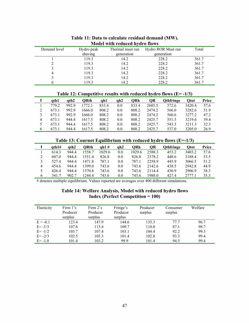
Table 11: Data to calculate residual demand (MW).

Model with reduced hydro flows Demand level Hydro peak

shaving Thermal must run

generation Hydro ROR Must run

generation Total

1 119.3 14.2 228.2 361.7 2 119.3 14.2 228.2 361.7 3 119.3 14.2 228.2 361.7 4 119.3 14.2 228.2 361.7 5 119.3 14.2 228.2 361.7 6 119.3 14.2 228.2 361.7

Table 12: Competitive results with reduced hydro flows (E= -1/3)

t qth1 qth2 QRth qh1 qh2 QRh QR Qthfringe Qtot Price 1 779.2 992.9 1772.1 833.4 0.0 833.4 2605.5 572.6 3420.4 57.6 2 673.1 992.9 1666.0 808.2 0.0 808.2 2474.2 566.0 3282.6 51.9 3 673.1 992.9 1666.0 808.2 0.0 808.2 2474.2 560.6 3277.2 47.2 4 673.1 944.4 1617.5 808.2 0.0 808.2 2425.7 551.5 3219.6 39.4 5 673.1 944.4 1617.5 808.2 0.0 808.2 2425.7 543.3 3211.3 32.3 6 673.1 944.4 1617.5 808.2 0.0 808.2 2425.7 537.0 3205.0 26.9

Table 13: Cournot Equilibrium with reduced hydro flows (E=-1/3)

t qth1# qth2 QRth qh1 # qh2 QRh QR Qthfringe Qtot Price 1 614.3 944.4 1558.7 1029.6 0.0 1029.6 2588.3 453.2 3403.2 57.6 2 607.0 944.4 1551.4 826.8 0.0 826.8 2378.2 448.6 3188.4 53.5 3 527.4 944.4 1471.8 787.1 0.0 787.1 2258.9 445.9 3066.5 51.2 4 454.6 944.4 1399.0 743.6 0.0 743.6 2142.6 438.5 2942.8 44.9 5 426.4 944.4 1370.8 743.6 0.0 743.6 2114.4 430.9 2906.9 38.3 6 341.7 902.7 1244.4 743.6 0.0 743.6 1988.0 427.4 2777.1 35.3

# denotes multiple equilibrium. Values reported are averages over 400 different simulations.

Table 14: Welfare Analysis, Model with reduced hydro flows Index (Perfect Competition = 100)

Elasticity Firm 1’s

Producer surplus

Firm 2’s Producer surplus

Fringe’s Producer surplus

Producer surplus

Consumer surplus

Welfare

E = -0.1 123.4 147.9 144.6 135.3 77.7 96.7 E= -1/3 107.6 115.4 109.7 110.0 87.1 98.7 E= -1/2 103.7 107.4 103.1 104.4 92.2 99.3 E= -2/3 102.5 105.3 101.4 102.8 93.3 99.4 E= -1.0 101.4 103.2 99.9 101.4 94.5 99.4

47

Table 15: Demand Indicators Total

demand (GWh)

Demand - qMR

(GWh) * Inflows (GWh)

Inflows (demand – qMR)

Average Net demand per day (GWh)

Max demand Min demand

Average Elasticity Residual Ddand

January 2733.43 2293.80 1058.98 46% 74.0 2.20 0.49 February 2520.23 2139.77 996.86 47% 76.4 1.90 0.47 March 2911.54 2532.46 1333.09 53% 81.7 1.85 0.51 April 2768.74 2484.73 1118.05 45% 82.8 2.00 0.48 May 2885.11 2587.79 1294.28 50% 83.5 1.69 0.45 June 2794.75 2466.61 1561.06 63% 82.2 1.82 0.50 July 2820.53 2487.82 1475.91 59% 80.3 1.79 0.49 August 2799.88 2478.86 1384.18 56% 80.0 1.75 0.49 September 2649.14 2307.95 1262.55 55% 76.9 1.94 0.48 October 2770.69 2399.68 1478.88 62% 77.4 1.93 0.40 November 2751.61 2328.93 1385.07 59% 77.6 1.90 0.40 December 2859.66 2410.97 1279.78 53% 77.8 1.98 0.40 * qMR includes production from must run thermal plants and hydro production from ROR plants.

Table 16: Marginal Value of Water (MVW)

E = -0.1 E = -1/3 E= - 0.5 E = -2/3 E = -1.0

January 0.00 11.13 11.13 13.91 17.90 February 0.00 11.13 11.13 13.54 17.75 March 0.00 10.62 11.13 13.36 17.75 April 0.00 11.13 11.89 15.78 19.85 May 0.00 9.53 11.13 12.78 17.29 June 0.00 0.00 7.78 11.13 14.21 July 0.00 1.92 10.08 11.13 15.41 August 0.00 6.45 11.13 11.13 15.78 September 0.00 8.47 11.13 11.98 17.03 October 0.00 0.00 9.82 11.13 15.78 November 0.00 2.21 11.13 11.13 17.01 December 0.00 9.88 11.13 14.61 20.28

48

Table 17: Marginal Value of Water under different price elasticity assumptions.

(1) (2) (3) (4) (1) (2) (3) (4) (1) (2) (3) (4) (1) (2) (3) Jan 11.13 10.08 0.00 0.00 0.49 0.49 0.15 0.15 0.10 0.0 0.03 0.0 46% 110% 46% Feb 11.13 9.33 17.75 17.25 0.47 0.47 1.36 1.36 0.08 0.0 0.23 0.0 47% 25% 47% Mar 10.62 8.88 0.00 0.00 0.51 0.51 0.15 0.15 0.08 0.0 0.03 0.0 53% 131% 53% Apr 11.13 11.13 15.78 15.45 0.48 0.48 0.94 0.94 0.10 0.0 0.19 0.0 45% 35% 45% May 9.53 7.85 9.53 7.85 0.45 0.45 0.45 0.45 0.06 0.0 0.06 0.0 50% 63% 50% Jun 0.00 0.00 0.00 0.00 0.50 0.50 0.50 0.50 0.09 0.0 0.09 0.0 63% 84% 63% Jul 1.92 1.14 1.92 1.14 0.49 0.49 0.49 0.49 0.08 0.0 0.08 0.0 59% 81% 59% Aug 6.45 5.32 11.13 11.13 0.49 0.49 0.73 0.73 0.09 0.0 0.13 0.0 56% 60% 56% Sep 8.47 7.02 11.98 11.13 0.48 0.48 0.92 0.92 0.09 0.0 0.16 0.0 55% 45% 55% Oct 0.00 0.00 11.13 11.13 0.40 0.40 0.72 0.72 0.06 0.0 0.11 0.0 62% 50% 62% Nov 2.21 1.08 17.01 16.62 0.40 0.40 1.00 1.00 0.06 0.0 0.12 0.0 59% 35% 59% Dec 9.88 7.90 14.61 14.02 0.40 0.40 0.72 0.72 0.06 0.0 0.09 0.0 53% 44% 53% Average 6.87 5.81 9.24 8.81 0.46 0.46 0.68 0.68 0.08 0.0 0.11 0.0 stdev 4.55 4.16 6.93 6.83 0.04 0.04 0.35 0.35 0.02 0.06 Corr MVW 0.24 0.27 0.88 0.89 0.26 0.77 -0.93 -0.22

MVW Average Elasticity of residual demand

St dev intra-month elasticity

Inflows/ net demand

Table 18:

Installed capacity in the SIC after full divestiture of Firm 1’s thermal plants (MW) Economic Group Thermal Hydro-reservoir Total Triopoly Endesa (Firm 1) 0 2454 2454 Gener (Firm 2) 1212 0 1212 Firm 3 939 0 939 Fringe 472 697 1169 DLTF Endesa (Firm 1) 0 2454 2454 Gener (Firm 2) 1212 0 1212 Fringe 1411 697 2108 Total 2622 3151 5773

Hydro-ROR not included in the table.

Table 19: Divestiture of Firm 1’s thermal plants - Triopoly (E=-1/3) t

qth1 qth2 qth3 QRth qh1 qh2 QRh QR QTh

Fringe Qtot Price Ex-Firm 1’s

thermal 1 0.0 944.4 673.1 1617.5 1620.8 0.0 1620.8 3238.3 431.9 4339.3 39.2 673.1 2 0.0 944.4 572.2 1516.6 1506.6 0.0 1506.6 3023.2 429.4 4030.8 37.0 572.2 3 0.0 920.5 500.7 1421.2 1435.1 0.0 1435.1 2856.3 427.8 3862.3 35.6 500.7 4 0.0 786.6 454.6 1241.2 1301.2 0.0 1301.2 2542.4 424.8 3545.4 33.0 454.6 5 0.0 662.4 454.6 1117.0 1177.0 0.0 1177.0 2294.0 422.0 3294.3 30.6 454.6 6 0.0 568.3 454.6 1022.9 1083.0 0.0 1083.0 2105.8 419.9 3104.0 28.8 454.6

49

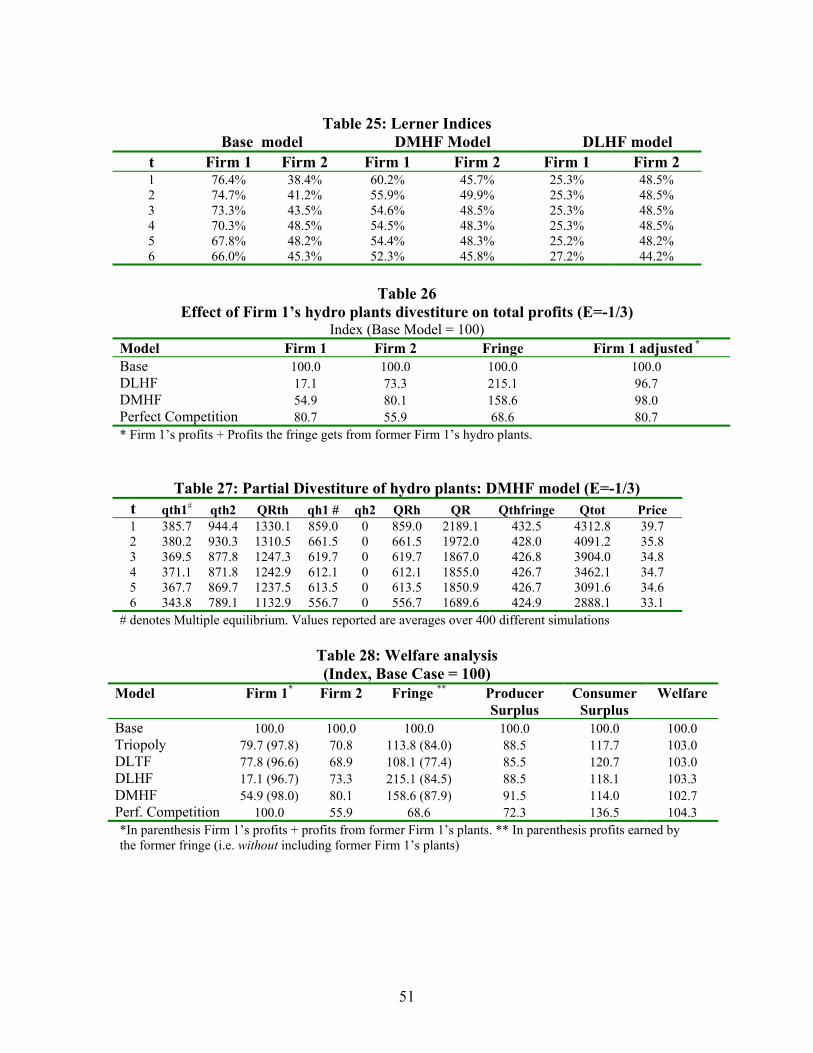
Table 25: Lerner Indices

Base model DMHF Model DLHF model t Firm 1 Firm 2 Firm 1 Firm 2 Firm 1 Firm 2 1 76.4% 38.4% 60.2% 45.7% 25.3% 48.5% 2 74.7% 41.2% 55.9% 49.9% 25.3% 48.5% 3 73.3% 43.5% 54.6% 48.5% 25.3% 48.5% 4 70.3% 48.5% 54.5% 48.3% 25.3% 48.5% 5 67.8% 48.2% 54.4% 48.3% 25.2% 48.2% 6 66.0% 45.3% 52.3% 45.8% 27.2% 44.2%

Table 26

Effect of Firm 1’s hydro plants divestiture on total profits (E=-1/3) Index (Base Model = 100)

Model Firm 1 Firm 2 Fringe Firm 1 adjusted *

Base 100.0 100.0 100.0 100.0 DLHF 17.1 73.3 215.1 96.7 DMHF 54.9 80.1 158.6 98.0 Perfect Competition 80.7 55.9 68.6 80.7 * Firm 1’s profits + Profits the fringe gets from former Firm 1’s hydro plants.

Table 27: Partial Divestiture of hydro plants: DMHF model (E=-1/3) t qth1# qth2 QRth qh1 # qh2 QRh QR Qthfringe Qtot Price 1 385.7 944.4 1330.1 859.0 0 859.0 2189.1 432.5 4312.8 39.7 2 380.2 930.3 1310.5 661.5 0 661.5 1972.0 428.0 4091.2 35.8 3 369.5 877.8 1247.3 619.7 0 619.7 1867.0 426.8 3904.0 34.8 4 371.1 871.8 1242.9 612.1 0 612.1 1855.0 426.7 3462.1 34.7 5 367.7 869.7 1237.5 613.5 0 613.5 1850.9 426.7 3091.6 34.6 6 343.8 789.1 1132.9 556.7 0 556.7 1689.6 424.9 2888.1 33.1

# denotes Multiple equilibrium. Values reported are averages over 400 different simulations

Table 28: Welfare analysis (Index, Base Case = 100)

Model Firm 1* Firm 2 Fringe ** Producer Surplus

Consumer Surplus

Welfare

Base 100.0 100.0 100.0 100.0 100.0 100.0 Triopoly 79.7 (97.8) 70.8 113.8 (84.0) 88.5 117.7 103.0 DLTF 77.8 (96.6) 68.9 108.1 (77.4) 85.5 120.7 103.0 DLHF 17.1 (96.7) 73.3 215.1 (84.5) 88.5 118.1 103.3 DMHF 54.9 (98.0) 80.1 158.6 (87.9) 91.5 114.0 102.7 Perf. Competition 100.0 55.9 68.6 72.3 136.5 104.3 *In parenthesis Firm 1’s profits + profits from former Firm 1’s plants. ** In parenthesis profits earned by the former fringe (i.e. without including former Firm 1’s plants)

51

Table 29: Cournot Equilibrium, Contracting level = 0% (E=-1/3) t K1 K2 qth1# qth2 QRth qh1 # qh2 QRh QR Qthfringe Qtot Price 1 0 0 133.7 944.4 1078.1 1743.0 0.0 1743.0 2821.3 441.2 3931.3 47.2 2 0 0 140.1 944.4 1084.5 1572.0 0.0 1572.0 2656.5 437.5 3672.3 44.0 3 0 0 120.3 944.4 1064.7 1472.6 0.0 1472.6 2537.3 434.9 3550.4 41.7 4 0 0 122.0 944.4 1066.4 1247.0 0.0 1247.0 2313.4 429.9 3321.5 37.4 5 0 0 127.0 867.7 994.7 1094.1 0.0 1094.1 2088.7 426.6 3093.6 34.6 6 0 0 131.9 773.6 905.4 995.1 0.0 995.1 1900.6 424.5 2903.3 32.8 # denotes Multiple equilibrium. Values reported are averages over 400 different simulations

Table 30: Cournot Equilibrium, Contracting level =50% (E=-1/3) t K1 K2 qth1 qth2 QRth qh1 qh2 QRh QR Qthfringe Qtot Price 1 1403.1 472.2 454.6 944.4 1399.0 1967.6 0.0 1967.6 3366.5 429.1 4464.4 36.7 2 1237.8 472.2 454.6 944.4 1399.0 1720.1 0.0 1720.1 3119.1 427.2 4124.6 35.1 3 1118.6 472.2 454.6 944.4 1399.0 1541.3 0.0 1541.3 2940.2 425.9 3944.4 34.0 4 894.7 472.2 454.6 944.4 1399.0 1205.4 0.0 1205.4 2604.4 423.4 3606.1 31.8 5 718.9 472.2 454.6 944.4 1399.0 931.3 0.0 931.3 2330.2 421.2 3329.7 29.9 6 655.0 472.2 454.6 944.4 1399.0 758.2 0.0 758.2 2157.1 418.8 3154.2 27.8

Table 31: Cournot Equilibrium, Contracting level =100% (E=-1/3) t K1 K2 qth1 qth2 QRth qh1 qh2 QRh QR Qthfringe Qtot Price 1 2806.2 944.4 673.1 944.4 1617.5 2134.7 0.0 2134.7 3752.2 420.5 4841.4 29.3 2 2475.7 944.4 673.1 944.4 1617.5 1804.6 0.0 1804.6 3422.1 420.5 4420.9 29.3 3 2237.2 944.4 673.1 944.4 1617.5 1566.2 0.0 1566.2 3183.6 420.5 4182.4 29.3 4 1789.4 944.4 673.1 944.4 1617.5 1118.4 0.0 1118.4 2735.8 420.5 3734.6 29.3 5 1437.8 944.4 673.1 944.4 1617.5 756.3 0.0 756.3 2373.8 420.3 3372.3 29.1 6 1310.0 944.4 566.4 944.4 1510.8 743.6 0.0 743.6 2254.4 416.6 3249.2 26.0

Table 32: Marginal Value of water (Ω1) Contracting Level

T 0% 50% 100% 1 11.13 17.13 29.27 2 11.13 17.13 29.27 3 11.13 17.13 29.27 4 11.13 17.13 29.27 5 11.13 17.13 29.27 6 11.13 17.13 25.98

Table 33: Lerner Indices

Contracting = 0% Contracting = 50% Contracting = 100% t Firm 1 Firm 2 Firm 1 Firm 2 Firm 1 Firm 2 1 76.4% 38.4% 53.3% 24.7% 0% 0% 2 74.7% 41.2% 51.2% 25.8% 0% 0% 3 73.3% 43.5% 49.6% 26.7% 0% 0% 4 70.3% 48.5% 46.2% 28.5% 0% 0% 5 67.8% 48.2% 42.8% 30.3% -1% 0% 6 66.0% 45.3% 38.5% 32.6% 0% 0%

52

Figures

Figure 1

Marginal Cost Functions

0

20

40

60

80

100

120

0 200 400 600 800 1000 1200

Adjusted Capacity, MW

US$

/ MW

Firm 1

Firm 2

Firm 3

Figure 2

Marginal Cost Functions

0

20

40

60

80

100

120

0 200 400 600 800 1000 1200 1400Adjusted capacity, MW

US$

/MW

Firm 1Fringe Firm 2

53

Figure 3

Load per hour (April 2000)

20002500300035004000450050005500

1 101 201 301 401 501 601 701Hour

MW

Figure 4

Anchor price/quantity

10

15

20

25

30

35

2500 3000 3500 4000 4500 5000

Output (MW)

pric

e

t=1

t=2

t=3

t=4

t=5

t=6

54

Figure 5

Fringe's MC if 2 strategic producers

0

10

20

30

40

50

60

0 100 200 300 400 500Capacity, MW

$/M

W

Figure 6

Peak shaving results (April 2000)

0

1000

2000

3000

4000

5000

6000

1 40 79 118

157

196

235

274

313

352

391

430

469

508

547

586

625

664

703

Ranking (hour)

MW

Load curve

Shaved demand

Hydro generation

55

Figure 9

Price

25

30

35

40

45

50

1 2 3 4 5 6

$/M

WCournot, E= -1/3

Cournot, E=-2/3

PC, E=-2/3

PC, E=-1/3

Figure 10 Total production

2500

3000

3500

4000

4500

5000

1 2 3 4 5 6

MW

Base, E= -1/3

Base, E=-2/3 PC

57

Figure 11

Firm 1's hydro production

0

500

1000

1500

2000

2500

1 2 3 4 5 6

MW Base, E=-1/3

Base, E=-2/3

PC

Figure 12

Firm 2's thermal production

600

700

800

900

1000

1 2 3 4 5 6

MW

Base, E= -1/3

PC

Base, E=-2/3

58

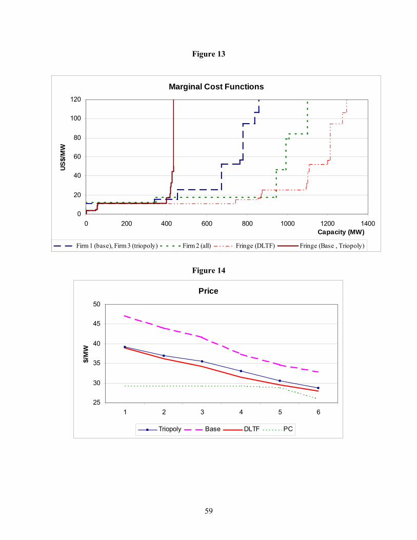
Figure 13

Marginal Cost Functions

0

20

40

60

80

100

120

0 200 400 600 800 1000 1200 1400Capacity (MW)

US$/

MW

Firm 1 (base), Firm 3 (triopoly) Firm 2 (all) Fringe (DLTF) Fringe (Base , Triopoly)

Figure 14

Price

25

30

35

40

45

50

1 2 3 4 5 6

$/M

W

Triopoly Base DLTF PC

59

Figure 15

Total Output

2800

3300

3800

4300

4800

1 2 3 4 5 6

MW

Triopoly Base DLTF PC

Figure 16

Firm 1's hydro production

700

900

1100

1300

1500

1700

1900

2100

1 2 3 4 5 6

MW

Triopoly Base DLTF PC

60

Figure 17

Firm 2's output

500

600

700

800

900

1000

1 2 3 4 5 6

MW

Triopoly Base DLTF PC

Figure 18

(Former) Firm 1's Thermal plants

0

200

400

600

800

1000

1 2 3 4 5 6

MW

Triopoly Base DLTF PC

61

Figure 19 Ba

qh1+qth2

1500170019002100230025002700290031003300

1 2 3 4 5 6

MW

Triopoly se DLTF PC

Figure 20

Peak shaving results (April 2000)

0

1000

2000

3000

4000

5000

6000

1 37 73 109

145

181

217

253

289

325

361

397

433

469

505

541

577

613

649

685

Ranking (hour)

MW

Load per hour Shaved demand - DLHF Shaved demand - base

Load per hour

Shaved demand (Base Model)

Shaved demand (DLHF)

62

Figure 21 2

Residual demand, DLHF model

0

5

10

15

20

25

30

35

40

1000 1500 2000 500 3000 3500 4000Output, MW

$/M

W

1 2 3 4 5 6

Figure 22

Price ($/MW)

0

10

20

30

40

50

1 2 3 4 5 6Base DLHF PC DMHF

63

Figure 23

Total Output, MW

01000

20003000

40005000

6000

1 2 3 4 5 6Base DLHF PC DMHF

Figure 24

Firm 1's thermal production (MW)

0

200

400

600

800

1 2 3 4 5 6Base DLHF PC DMHF

64

Figure 25

Firm 2's thermal production (MW)

600

700

800

900

1000

1 2 3 4 5 6Base DLHF PC DMHF

Figure 26

Former Firm 1 hydro-plants' production, MW

0

500

1000

1500

2000

2500

1 2 3 4 5 6Base DLHF PC DMHF

65

Figure 27

Fringe's thermal production (MW)

400

410

420

430

440

450

1 2 3 4 5 6Base DLHF PC DMHF

Figure 28

Pr

ice

15

20

25

30

35

40

45

1 2 3 4 5 6

$/M

W

0%

50%

100% , PC

66

Figure 29

Total production by Cournot producers

1500

2000

2500

3000

3500

4000

1 2 3 4 5 6

MW

PC, 100%

50%

0%

Figure 30

Firm 1 hydro's generation

500700900

1100130015001700190021002300

1 2 3 4 5 6

MW

0% 50% 100% PC

67

Figure 31

Firm 2's production

500

600

700

800

900

1000

1 2 3 4 5 6

0%

50%

100%, PC

Figure 32

50%

Firm 1's total production

1000120014001600180020002200240026002800

1 2 3 4 5 6

MW

0% 100% PC

68

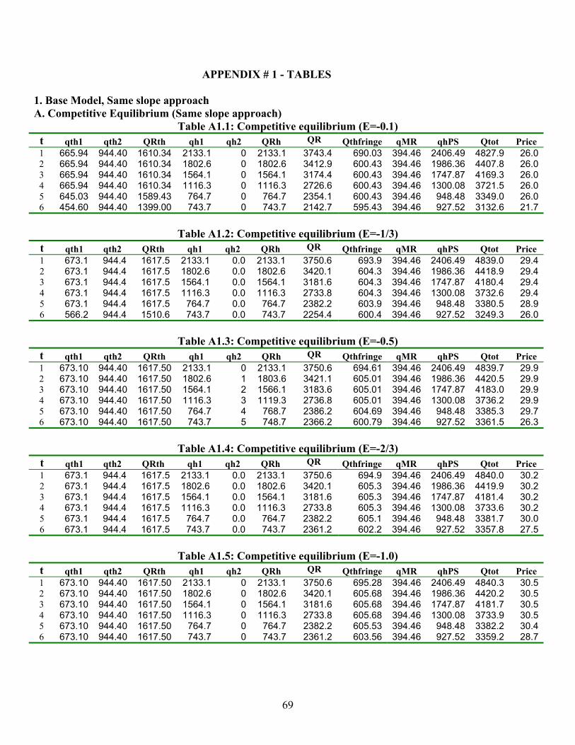
APPENDIX # 1 - TABLES

1. Base Model, Same slope approach A. Competitive Equilibrium (Same slope approach)

Table A1.1: Competitive equilibrium (E=-0.1) t qth1 qth2 QRth qh1 qh2 QRh QR Qthfringe qMR qhPS Qtot Price 1 665.94 944.40 1610.34 2133.1 0 2133.1 3743.4 690.03 394.46 2406.49 4827.9 26.02 665.94 944.40 1610.34 1802.6 0 1802.6 3412.9 600.43 394.46 1986.36 4407.8 26.03 665.94 944.40 1610.34 1564.1 0 1564.1 3174.4 600.43 394.46 1747.87 4169.3 26.04 665.94 944.40 1610.34 1116.3 0 1116.3 2726.6 600.43 394.46 1300.08 3721.5 26.05 645.03 944.40 1589.43 764.7 0 764.7 2354.1 600.43 394.46 948.48 3349.0 26.06 454.60 944.40 1399.00 743.7 0 743.7 2142.7 595.43 394.46 927.52 3132.6 21.7

Table A1.2: Competitive equilibrium (E=-1/3)

t qth1 qth2 QRth qh1 qh2 QRh QR Qthfringe qMR qhPS Qtot Price 1 673.1 944.4 1617.5 2133.1 0.0 2133.1 3750.6 693.9 394.46 2406.49 4839.0 29.42 673.1 944.4 1617.5 1802.6 0.0 1802.6 3420.1 604.3 394.46 1986.36 4418.9 29.43 673.1 944.4 1617.5 1564.1 0.0 1564.1 3181.6 604.3 394.46 1747.87 4180.4 29.44 673.1 944.4 1617.5 1116.3 0.0 1116.3 2733.8 604.3 394.46 1300.08 3732.6 29.45 673.1 944.4 1617.5 764.7 0.0 764.7 2382.2 603.9 394.46 948.48 3380.5 28.96 566.2 944.4 1510.6 743.7 0.0 743.7 2254.4 600.4 394.46 927.52 3249.3 26.0

Table A1.3: Competitive equilibrium (E=-0.5)

t qth1 qth2 QRth qh1 qh2 QRh QR Qthfringe qMR qhPS Qtot Price 1 673.10 944.40 1617.50 2133.1 0 2133.1 3750.6 694.61 394.46 2406.49 4839.7 29.92 673.10 944.40 1617.50 1802.6 1 1803.6 3421.1 605.01 394.46 1986.36 4420.5 29.93 673.10 944.40 1617.50 1564.1 2 1566.1 3183.6 605.01 394.46 1747.87 4183.0 29.94 673.10 944.40 1617.50 1116.3 3 1119.3 2736.8 605.01 394.46 1300.08 3736.2 29.95 673.10 944.40 1617.50 764.7 4 768.7 2386.2 604.69 394.46 948.48 3385.3 29.76 673.10 944.40 1617.50 743.7 5 748.7 2366.2 600.79 394.46 927.52 3361.5 26.3

Table A1.4: Competitive equilibrium (E=-2/3)

t qth1 qth2 QRth qh1 qh2 QRh QR Qthfringe qMR qhPS Qtot Price 1 673.1 944.4 1617.5 2133.1 0.0 2133.1 3750.6 694.9 394.46 2406.49 4840.0 30.22 673.1 944.4 1617.5 1802.6 0.0 1802.6 3420.1 605.3 394.46 1986.36 4419.9 30.23 673.1 944.4 1617.5 1564.1 0.0 1564.1 3181.6 605.3 394.46 1747.87 4181.4 30.24 673.1 944.4 1617.5 1116.3 0.0 1116.3 2733.8 605.3 394.46 1300.08 3733.6 30.25 673.1 944.4 1617.5 764.7 0.0 764.7 2382.2 605.1 394.46 948.48 3381.7 30.06 673.1 944.4 1617.5 743.7 0.0 743.7 2361.2 602.2 394.46 927.52 3357.8 27.5

Table A1.5: Competitive equilibrium (E=-1.0)

t qth1 qth2 QRth qh1 qh2 QRh QR Qthfringe qMR qhPS Qtot Price 1 673.10 944.40 1617.50 2133.1 0 2133.1 3750.6 695.28 394.46 2406.49 4840.3 30.52 673.10 944.40 1617.50 1802.6 0 1802.6 3420.1 605.68 394.46 1986.36 4420.2 30.53 673.10 944.40 1617.50 1564.1 0 1564.1 3181.6 605.68 394.46 1747.87 4181.7 30.54 673.10 944.40 1617.50 1116.3 0 1116.3 2733.8 605.68 394.46 1300.08 3733.9 30.55 673.10 944.40 1617.50 764.7 0 764.7 2382.2 605.53 394.46 948.48 3382.2 30.46 673.10 944.40 1617.50 743.7 0 743.7 2361.2 603.56 394.46 927.52 3359.2 28.7

69

B. Cournot equilibrium (Same slope approach)

Table A1.6: Cournot equilibrium (E=-0.1) t qth1 # qth2 QRth qh1 # qh2 QRh QR Qthfringe qMR qhPS Qtot Price 1 0.0 944.4 944.4 1612.3 0.0 1612.3 2556.7 500.3 394.46 274.6 3726.1 98.12 0.0 944.4 944.4 1447.7 0.0 1447.7 2392.1 488.6 394.46 183.8 3459.0 88.13 0.0 944.4 944.4 1328.4 0.0 1328.4 2272.8 480.2 394.46 183.8 3331.3 80.94 0.0 854.9 854.9 1149.3 0.0 1149.3 2004.2 467.6 394.46 183.8 3050.0 70.05 0.0 730.7 730.7 1025.1 0.0 1025.1 1755.9 458.8 394.46 183.8 2792.9 62.46 0.0 636.6 636.6 931.0 0.0 931.0 1567.7 452.2 394.46 183.8 2598.1 56.7

# denotes multiple equilibrium. Values reported are averages over 400 simulations.

Table A1.7: Cournot equilibrium (E=-1/3) t qth1 # qth2 QRth qh1 # qh2 QRh QR Qthfringe qMR qhPS Qtot Price 1 133.7 944.4 1078.1 1743.0 0.0 1743.0 2821.1 441.2 394.46 274.6 3931.4 47.22 140.1 944.4 1084.5 1572.0 0.0 1572.0 2656.5 437.5 394.46 183.8 3672.3 44.03 120.3 944.4 1064.7 1472.6 0.0 1472.6 2537.3 434.9 394.46 183.8 3550.4 41.74 122.0 944.4 1066.4 1247.0 0.0 1247.0 2313.4 429.9 394.46 183.8 3321.5 37.45 127.0 867.7 994.7 1094.1 0.0 1094.1 2088.8 426.6 394.46 183.8 3093.6 34.66 131.9 773.6 905.4 995.1 0.0 995.1 1900.6 424.5 394.46 183.8 2903.3 32.8

# denotes multiple equilibrium. Values reported are averages over 400 simulations.

Table A1.8: Cournot equilibrium (E=-0.5) t qth1 # qth2 QRth qh1 # qh2 QRh QR Qthfringe qMR qhPS Qtot Price 1 341.7 944.4 1286.1 1759.9 0.0 1759.9 3046.0 431.7 394.46 274.6 4146.8 39.02 341.7 944.4 1286.1 1595.3 0.0 1595.3 2881.4 429.3 394.46 183.8 3888.9 36.93 341.7 944.4 1286.1 1476.0 0.0 1476.0 2762.1 427.5 394.46 183.8 3767.8 35.34 341.7 944.4 1286.1 1252.1 0.0 1252.1 2538.2 424.1 394.46 183.8 3540.6 32.45 341.7 941.5 1283.2 1067.3 0.0 1067.3 2350.5 421.4 394.46 183.8 3350.1 30.16 341.7 847.4 1189.1 973.2 0.0 973.2 2162.3 420.0 394.46 183.8 3160.5 28.9

# denotes multiple equilibrium. Values reported are averages over 400 simulations.

Table A1.9:Cournot equilibrium (E=-2/3) t qth1 # qth2 QRth qh1 # qh2 QRh QR Qthfringe qMR qhPS Qtot Price 1 377.7 944.4 1322.1 1768.1 0.0 1768.1 3090.2 429.0 394.46 274.6 4188.3 36.62 376.0 944.4 1320.4 1605.2 0.0 1605.2 2925.6 427.1 394.46 183.8 3930.9 35.03 378.3 944.4 1322.7 1483.6 0.0 1483.6 2806.3 425.8 394.46 183.8 3810.3 33.94 375.8 944.4 1320.2 1262.2 0.0 1262.2 2582.4 423.2 394.46 183.8 3583.9 31.75 379.6 944.4 1324.0 1072.2 0.0 1072.2 2396.2 421.1 394.46 183.8 3395.6 29.96 378.2 944.4 1322.5 932.5 0.0 932.5 2255.0 419.6 394.46 183.8 3252.8 28.5

# denotes multiple equilibrium. Values reported are averages over 400 simulations.

Table A1.10: Cournot equilibrium (E=-1.0) t qth1# qth2 QRth qh1 # qh2 QRh QR Qthfringe qMR qhPS Qtot Price 1 454.6 944.4 1399.0 1768.2 0.0 1768.2 3167.2 426.3 394.46 274.6 4262.5 34.32 454.6 944.4 1399.0 1603.6 0.0 1603.6 3002.6 425.0 394.46 183.8 4005.8 33.23 454.6 944.4 1399.0 1484.3 0.0 1484.3 2883.3 424.1 394.46 183.8 3885.7 32.44 454.6 944.4 1399.0 1260.4 0.0 1260.4 2659.4 422.4 394.46 183.8 3660.1 31.05 454.6 944.4 1399.0 1074.2 0.0 1074.2 2473.2 421.0 394.46 183.8 3472.4 29.86 454.6 944.4 1399.0 933.0 0.0 933.0 2332.0 420.0 394.46 183.8 3330.2 28.9

# denotes multiple equilibrium. Values reported are averages over 400 simulations.

70

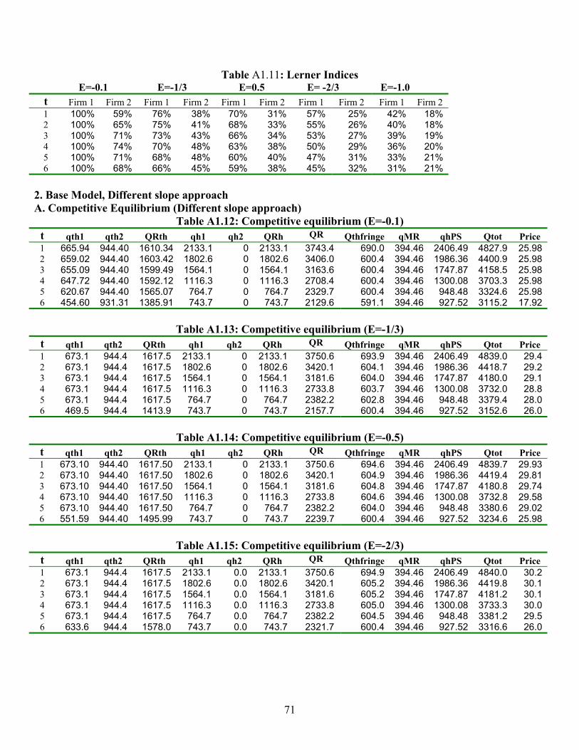
Table A1.11: Lerner Indices E=-0.1 E=-1/3 E=0.5 E= -2/3 E=-1.0

t Firm 1 Firm 2 Firm 1 Firm 2 Firm 1 Firm 2 Firm 1 Firm 2 Firm 1 Firm 2 1 100% 59% 76% 38% 70% 31% 57% 25% 42% 18% 2 100% 65% 75% 41% 68% 33% 55% 26% 40% 18% 3 100% 71% 73% 43% 66% 34% 53% 27% 39% 19% 4 100% 74% 70% 48% 63% 38% 50% 29% 36% 20% 5 100% 71% 68% 48% 60% 40% 47% 31% 33% 21% 6 100% 68% 66% 45% 59% 38% 45% 32% 31% 21%

2. Base Model, Different slope approach A. Competitive Equilibrium (Different slope approach)

Table A1.12: Competitive equilibrium (E=-0.1) t qth1 qth2 QRth qh1 qh2 QRh QR Qthfringe qMR qhPS Qtot Price 1 665.94 944.40 1610.34 2133.1 0 2133.1 3743.4 690.0 394.46 2406.49 4827.9 25.982 659.02 944.40 1603.42 1802.6 0 1802.6 3406.0 600.4 394.46 1986.36 4400.9 25.983 655.09 944.40 1599.49 1564.1 0 1564.1 3163.6 600.4 394.46 1747.87 4158.5 25.984 647.72 944.40 1592.12 1116.3 0 1116.3 2708.4 600.4 394.46 1300.08 3703.3 25.985 620.67 944.40 1565.07 764.7 0 764.7 2329.7 600.4 394.46 948.48 3324.6 25.986 454.60 931.31 1385.91 743.7 0 743.7 2129.6 591.1 394.46 927.52 3115.2 17.92

Table A1.13: Competitive equilibrium (E=-1/3)

t qth1 qth2 QRth qh1 qh2 QRh QR Qthfringe qMR qhPS Qtot Price 1 673.1 944.4 1617.5 2133.1 0 2133.1 3750.6 693.9 394.46 2406.49 4839.0 29.42 673.1 944.4 1617.5 1802.6 0 1802.6 3420.1 604.1 394.46 1986.36 4418.7 29.23 673.1 944.4 1617.5 1564.1 0 1564.1 3181.6 604.0 394.46 1747.87 4180.0 29.14 673.1 944.4 1617.5 1116.3 0 1116.3 2733.8 603.7 394.46 1300.08 3732.0 28.85 673.1 944.4 1617.5 764.7 0 764.7 2382.2 602.8 394.46 948.48 3379.4 28.06 469.5 944.4 1413.9 743.7 0 743.7 2157.7 600.4 394.46 927.52 3152.6 26.0

Table A1.14: Competitive equilibrium (E=-0.5)

t qth1 qth2 QRth qh1 qh2 QRh QR Qthfringe qMR qhPS Qtot Price 1 673.10 944.40 1617.50 2133.1 0 2133.1 3750.6 694.6 394.46 2406.49 4839.7 29.932 673.10 944.40 1617.50 1802.6 0 1802.6 3420.1 604.9 394.46 1986.36 4419.4 29.813 673.10 944.40 1617.50 1564.1 0 1564.1 3181.6 604.8 394.46 1747.87 4180.8 29.744 673.10 944.40 1617.50 1116.3 0 1116.3 2733.8 604.6 394.46 1300.08 3732.8 29.585 673.10 944.40 1617.50 764.7 0 764.7 2382.2 604.0 394.46 948.48 3380.6 29.026 551.59 944.40 1495.99 743.7 0 743.7 2239.7 600.4 394.46 927.52 3234.6 25.98

Table A1.15: Competitive equilibrium (E=-2/3)

t qth1 qth2 QRth qh1 qh2 QRh QR Qthfringe qMR qhPS Qtot Price 1 673.1 944.4 1617.5 2133.1 0.0 2133.1 3750.6 694.9 394.46 2406.49 4840.0 30.22 673.1 944.4 1617.5 1802.6 0.0 1802.6 3420.1 605.2 394.46 1986.36 4419.8 30.13 673.1 944.4 1617.5 1564.1 0.0 1564.1 3181.6 605.2 394.46 1747.87 4181.2 30.14 673.1 944.4 1617.5 1116.3 0.0 1116.3 2733.8 605.0 394.46 1300.08 3733.3 30.05 673.1 944.4 1617.5 764.7 0.0 764.7 2382.2 604.5 394.46 948.48 3381.2 29.56 633.6 944.4 1578.0 743.7 0.0 743.7 2321.7 600.4 394.46 927.52 3316.6 26.0

71

Table A1.16: Competitive equilibrium (E=-1.0) t qth1 qth2 QRth qh1 qh2 QRh QR Qthfringe qMR qhPS Qtot Price 1 673.10 944.40 1617.50 2133.1 0 2133.1 3750.6 695.3 394.46 2406.49 4840.3 30.512 673.10 944.40 1617.50 1802.6 0 1802.6 3420.1 605.6 394.46 1986.36 4420.1 30.453 673.10 944.40 1617.50 1564.1 0 1564.1 3181.6 605.6 394.46 1747.87 4181.6 30.424 673.10 944.40 1617.50 1116.3 0 1116.3 2733.8 605.5 394.46 1300.08 3733.7 30.335 673.10 944.40 1617.50 764.7 0 764.7 2382.2 605.1 394.46 948.48 3381.8 30.056 673.10 944.40 1617.50 743.7 0 743.7 2361.2 601.9 394.46 927.52 3357.6 27.26

B. Cournot equilibrium (Different slope approach)

Table A1.17: Cournot equilibrium (E=-0.1) t qth1 # qth2 QRth qh1 # qh2 QRh QR Qthfringe qMR qhPS Qtot Price 1 0.0 944.4 944.4 1612.3 0.0 1612.3 2556.7 500.1 394.46 274.6 3725.9 98.02 0.0 944.4 944.4 1426.7 0.0 1426.7 2371.1 496.3 394.46 183.8 3445.6 94.73 0.0 944.4 944.4 1295.5 0.0 1295.5 2239.9 491.1 394.46 183.8 3309.2 90.24 0.0 860.7 860.7 1091.1 0.0 1091.1 1951.8 484.9 394.46 183.8 3014.9 84.95 0.0 738.4 738.4 947.3 0.0 947.3 1685.8 480.7 394.46 183.8 2744.7 81.36 0.0 645.7 645.7 838.4 0.0 838.4 1484.1 476.8 394.46 183.8 2539.2 77.9

# denotes multiple equilibrium. Values reported are averages over 400 simulations.

Table A1.18: Cournot equilibrium (E=-1/3) t qth1 # qth2 QRth qh1 # qh2 QRh QR Qthfringe qMR qhPS Qtot Price 1 61.2 944.4 1005.6 1815.6 0.0 1815.6 2821.2 441.2 394.46 274.6 3931.5 47.22 59.0 944.4 1003.4 1608.1 0.0 1608.1 2611.5 440.0 394.46 183.8 3629.8 46.23 49.7 944.4 994.0 1472.7 0.0 1472.7 2466.8 438.6 394.46 183.8 3483.6 45.04 31.4 944.4 975.7 1219.2 0.0 1219.2 2194.9 435.5 394.46 183.8 3208.6 42.25 21.1 833.9 855.0 1058.6 0.0 1058.6 1913.6 434.0 394.46 183.8 2925.8 40.96 9.0 733.3 742.3 949.6 0.0 949.6 1691.9 432.9 394.46 183.8 2703.1 40.0

# denotes multiple equilibrium. Values reported are averages over 400 simulations.

Table A1.19: Cournot equilibrium (E=-0.5) t qth1 # qth2 QRth qh1 # qh2 QRh QR Qthfringe qMR qhPS Qtot Price 1 248.6 944.4 1193.0 1882.4 0.0 1882.4 3075.4 431.3 394.46 274.6 4175.7 38.62 241.2 944.4 1185.6 1657.7 0.0 1657.7 2843.2 430.5 394.46 183.8 3852.0 38.03 242.8 944.4 1187.2 1498.5 0.0 1498.5 2685.7 429.6 394.46 183.8 3693.5 37.14 232.2 944.4 1176.6 1213.3 0.0 1213.3 2389.9 427.5 394.46 183.8 3395.6 35.35 259.0 871.2 1130.2 977.1 0.0 977.1 2107.3 426.1 394.46 183.8 3111.6 34.16 206.6 767.5 974.1 894.8 0.0 894.8 1868.9 425.4 394.46 183.8 2872.5 33.5

# denotes multiple equilibrium. Values reported are averages over 400 simulations.

Table A1.20: Cournot equilibrium (E=-2/3) t qth1 # qth2 QRth qh1 # qh2 QRh QR Qthfringe qMR qhPS Qtot Price 1 341.7 944.4 1286.1 1933.0 0.0 1933.0 3219.1 427.5 394.46 274.6 4315.7 35.42 341.7 944.4 1286.1 1688.1 0.0 1688.1 2974.2 426.9 394.46 183.8 3979.3 34.93 341.7 944.4 1286.1 1523.2 0.0 1523.2 2809.3 426.2 394.46 183.8 3813.8 34.34 341.7 944.4 1286.1 1213.8 0.0 1213.8 2499.9 424.7 394.46 183.8 3502.8 32.95 341.7 944.4 1286.1 956.4 0.0 956.4 2242.5 423.0 394.46 183.8 3243.7 31.56 341.7 848.2 1190.0 809.3 0.0 809.3 1999.3 422.4 394.46 183.8 2999.9 30.9

# denotes multiple equilibrium. Values reported are averages over 400 simulations.

72

Table A1.21: Cournot equilibrium (E=-1.0) t qth1 # qth2 QRth qh1 # qh2 QRh QR Qthfringe qMR qhPS Qtot Price 1 454.6 944.4 1399.0 1969.6 0.0 1969.6 3368.5 424.8 394.46 274.6 4462.4 33.02 454.6 944.4 1399.0 1711.2 0.0 1711.2 3110.2 424.4 394.46 183.8 4112.8 32.73 454.6 944.4 1399.0 1538.8 0.0 1538.8 2937.7 423.9 394.46 183.8 3939.9 32.34 454.6 944.4 1399.0 1215.0 0.0 1215.0 2614.0 422.8 394.46 183.8 3615.1 31.35 454.6 944.4 1399.0 945.7 0.0 945.7 2344.6 421.8 394.46 183.8 3344.6 30.46 454.6 944.4 1399.0 743.6 0.0 743.6 2142.6 420.7 394.46 183.8 3141.5 29.5

# denotes multiple equilibrium. Values reported are averages over 400 simulations.

Table A1.22: Lerner Indices E=-0.1 E=-1/3 E=0.5 E= -2/3 E=-1.0

t Firm 1 Firm 2 Firm 1 Firm 2 Firm 1 Firm 2 Firm 1 Firm 2 Firm 1 Firm 2 1 100% 59% 76% 38% 71% 32% 62% 26% 48% 19% 2 100% 66% 76% 43% 71% 35% 62% 29% 47% 21% 3 100% 73% 75% 47% 70% 38% 61% 31% 47% 22% 4 100% 79% 74% 56% 69% 45% 60% 36% 45% 25% 5 100% 78% 73% 56% 67% 48% 58% 42% 43% 29% 6 100% 77% 72% 55% 67% 47% 57% 42% 42% 33%

3. Base Model, Same slope approach, Reduced Hydro Flows A. Competitive Equilibrium (Same slope approach)

Table A1.23: Competitive equilibrium (E=-0.1) t qth1 qth2 QRth qh1 qh2 QRh QR Qthfringe qMR qhPS Qtot Price 1 860.0 1101.3 1961.3 833.4 0.0 833.4 2794.7 629.9 242.4 952.7 3666.9 107.02 779.2 1101.3 1880.5 808.2 0.0 808.2 2688.7 606.1 242.4 927.5 3537.1 86.53 779.2 992.9 1772.1 808.2 0.0 808.2 2580.3 596.2 242.4 927.5 3418.9 78.04 705.2 992.9 1698.1 808.2 0.0 808.2 2506.3 566.8 242.4 927.5 3315.4 52.65 673.1 944.4 1617.5 808.2 0.0 808.2 2425.7 546.2 242.4 927.5 3214.3 34.86 535.8 944.4 1480.2 808.2 0.0 808.2 2288.4 536.0 242.4 927.5 3066.7 26.0

Table A1.24: Competitive equilibrium (E=-1/3)

t qth1 qth2 QRth qh1 qh2 QRh QR Qthfringe qMR qhPS Qtot Price 1 779.2 992.9 1772.1 833.4 0.0 833.4 2605.5 572.6 242.4 952.7 3420.4 57.62 673.1 992.9 1666.0 808.2 0.0 808.2 2474.2 566.0 242.4 927.5 3282.6 51.93 673.1 992.9 1666.0 808.2 0.0 808.2 2474.2 560.6 242.4 927.5 3277.2 47.24 673.1 944.4 1617.5 808.2 0.0 808.2 2425.7 551.5 242.4 927.5 3219.6 39.45 673.1 944.4 1617.5 808.2 0.0 808.2 2425.7 543.3 242.4 927.5 3211.3 32.36 673.1 944.4 1617.5 808.2 0.0 808.2 2425.7 537.0 242.4 927.5 3205.0 26.9

Table A1.25: Competitive equilibrium (E=-0.5)

t qth1 qth2 QRth qh1 qh2 QRh QR Qthfringe qMR qhPS Qtot Price 1 673.1 992.9 1666.0 833.4 0.0 833.4 2499.4 564.0 242.4 952.7 3305.7 50.22 673.1 944.4 1617.5 808.2 0.0 808.2 2425.7 558.7 242.4 927.5 3226.8 45.63 673.1 944.4 1617.5 808.2 0.0 808.2 2425.7 555.1 242.4 927.5 3223.2 42.54 673.1 944.4 1617.5 808.2 0.0 808.2 2425.7 548.4 242.4 927.5 3216.4 36.75 673.1 944.4 1617.5 808.2 0.0 808.2 2425.7 542.8 242.4 927.5 3210.9 31.96 673.1 944.4 1617.5 808.2 0.0 808.2 2425.7 538.6 242.4 927.5 3206.6 28.2

73

Table A1.26: Competitive equilibrium (E=-2/3) t qth1 qth2 QRth qh1 qh2 QRh QR Qthfringe qMR qhPS Qtot Price 1 673.1 944.4 1617.5 833.4 0.0 833.4 2450.9 559.0 242.4 952.7 3252.3 45.92 673.1 944.4 1617.5 808.2 0.0 808.2 2425.7 554.5 242.4 927.5 3222.6 42.03 673.1 944.4 1617.5 808.2 0.0 808.2 2425.7 551.8 242.4 927.5 3219.9 39.74 673.1 944.4 1617.5 808.2 0.0 808.2 2425.7 546.8 242.4 927.5 3214.8 35.35 673.1 944.4 1617.5 808.2 0.0 808.2 2425.7 542.6 242.4 927.5 3210.6 31.76 673.1 944.4 1617.5 808.2 0.0 808.2 2425.7 539.4 242.4 927.5 3207.5 29.0

Table A1.27: Competitive equilibrium (E=-1.0)

t qth1 qth2 QRth qh1 qh2 QRh QR Qthfringe qMR qhPS Qtot Price 1 673.1 944.4 1617.5 833.4 0.0 833.4 2450.9 553.3 242.4 952.7 3246.5 40.92 673.1 944.4 1617.5 808.2 0.0 808.2 2425.7 550.3 242.4 927.5 3218.4 38.43 673.1 944.4 1617.5 808.2 0.0 808.2 2425.7 548.5 242.4 927.5 3216.6 36.84 673.1 944.4 1617.5 808.2 0.0 808.2 2425.7 545.2 242.4 927.5 3213.2 33.95 673.1 944.4 1617.5 808.2 0.0 808.2 2425.7 542.4 242.4 927.5 3210.4 31.56 673.1 944.4 1617.5 808.2 0.0 808.2 2425.7 540.2 242.4 927.5 3208.3 29.7

B. Cournot equilibrium, Same slope approach, Reduced Hydro Flows

Table A1.28: Cournot equilibrium (E=-0.1) t qth1 # qth2 QRth qh1 # qh2 QRh QR Qthfringe qMR qhPS Qtot Price 1 486.8 992.9 1479.8 1041.5 0.0 1041.5 2521.2 524.4 242.4 119.3 3407.4 119.02 488.9 983.0 1472.0 834.2 0.0 834.2 2306.2 510.0 242.4 119.3 3177.9 106.53 455.6 944.4 1399.9 767.8 0.0 767.8 2167.7 502.9 242.4 119.3 3032.3 100.44 341.7 944.4 1286.1 743.6 0.0 743.6 2029.7 481.1 242.4 119.3 2872.5 81.65 231.8 863.9 1095.7 743.6 0.0 743.6 1839.3 468.2 242.4 119.3 2669.2 70.56 137.7 769.8 907.5 743.6 0.0 743.6 1651.1 461.6 242.4 119.3 2474.4 64.8

# denotes multiple equilibrium. Values reported are averages over 400 simulations.

Table A1.29: Cournot equilibrium (E=-1/3) t qth1 # qth2 QRth qh1 # qh2 QRh QR Qthfringe qMR qhPS Qtot Price 1 614.3 944.4 1558.7 1029.6 0.0 1029.6 2588.3 453.2 242.4 119.3 3403.2 57.62 607.0 944.4 1551.4 826.8 0.0 826.8 2378.2 448.6 242.4 119.3 3188.4 53.53 527.4 944.4 1471.8 787.1 0.0 787.1 2258.9 445.9 242.4 119.3 3066.5 51.24 454.6 944.4 1399.0 743.6 0.0 743.6 2142.6 438.5 242.4 119.3 2942.8 44.95 426.4 944.4 1370.8 743.6 0.0 743.6 2114.4 430.9 242.4 119.3 2906.9 38.36 341.7 902.7 1244.4 743.6 0.0 743.6 1988.0 427.4 242.4 119.3 2777.1 35.3

# denotes multiple equilibrium. Values reported are averages over 400 simulations.

Table A1.30: Cournot equilibrium (E=-0.5) t qth1 # qth2 QRth qh1 # qh2 QRh QR Qthfringe qMR qhPS Qtot Price 1 662.7 944.4 1607.1 1046.3 0.0 1046.3 2653.4 442.2 242.4 119.3 3457.3 48.02 662.7 944.4 1607.1 836.3 0.0 836.3 2443.4 439.0 242.4 119.3 3244.1 45.33 618.9 944.4 1563.3 760.9 0.0 760.9 2324.1 437.3 242.4 119.3 3123.1 43.84 454.6 944.4 1399.0 743.6 0.0 743.6 2142.6 433.3 242.4 119.3 2937.6 40.35 454.6 944.4 1399.0 743.6 0.0 743.6 2142.6 427.7 242.4 119.3 2932.0 35.56 454.6 944.4 1399.0 743.6 0.0 743.6 2142.6 423.5 242.4 119.3 2927.8 31.9

# denotes multiple equilibrium. Values reported are averages over 400 simulations.

74

75

Table A1.31:Cournot equilibrium (E=-2/3) t qth1 # qth2 QRth qh1 # qh2 QRh QR Qthfringe qMR qhPS Qtot Price 1 673.1 944.4 1617.5 1055.0 0.0 1055.0 2672.4 437.1 242.4 119.3 3471.3 43.72 673.1 944.4 1617.5 844.9 0.0 844.9 2462.4 434.8 242.4 119.3 3258.8 41.63 673.1 944.4 1617.5 743.6 0.0 743.6 2361.1 433.2 242.4 119.3 3156.0 40.34 477.5 944.4 1421.8 743.6 0.0 743.6 2165.4 430.4 242.4 119.3 2957.5 37.85 454.6 944.4 1399.0 743.6 0.0 743.6 2142.6 426.4 242.4 119.3 2930.7 34.46 454.6 944.4 1399.0 743.6 0.0 743.6 2142.6 423.3 242.4 119.3 2927.5 31.7

# denotes multiple equilibrium. Values reported are averages over 400 simulations.

Table A1.32: Cournot equilibrium (E=-1.0) t qth1 # qth2 QRth qh1 # qh2 QRh QR Qthfringe qMR qhPS Qtot Price 1 673.1 944.4 1617.5 1055.0 0.0 1055.0 2672.4 432.3 242.4 119.3 3466.4 39.52 673.1 944.4 1617.5 844.9 0.0 844.9 2462.4 430.7 242.4 119.3 3254.8 38.13 673.1 944.4 1617.5 743.6 0.0 743.6 2361.1 429.7 242.4 119.3 3152.4 37.24 607.8 944.4 1552.2 743.6 0.0 743.6 2295.8 426.8 242.4 119.3 3084.3 34.85 454.6 944.4 1399.0 743.6 0.0 743.6 2142.6 425.2 242.4 119.3 2929.4 33.36 454.6 944.4 1399.0 743.6 0.0 743.6 2142.6 423.0 242.4 119.3 2927.3 31.5

# denotes multiple equilibrium. Values reported are averages over 400 simulations.

Table A1.33: Lerner Indices E=-0.1 E=-1/3 E=0.5 E= -2/3 E=-1.0

t Firm 1 Firm 2 Firm 1 Firm 2 Firm 1 Firm 2 Firm 1 Firm 2 Firm 1 Firm 2 1 78% 51% 55% 32% 46% 25% 38% 21% 28% 16% 2 76% 56% 51% 34% 43% 27% 35% 22% 26% 16% 3 74% 57% 49% 35% 41% 28% 34% 23% 25% 16% 4 81% 70% 51% 40% 38% 30% 31% 24% 25% 18% 5 84% 75% 59% 47% 43% 34% 34% 27% 23% 18% 6 83% 72% 59% 49% 48% 38% 37% 29% 25% 19%

12 Appendix 2: A simple 1-year Cournot Model forChile’s Electricity Industry

The model that was used to analyze the exercise of market power in Chile’s electricity industryassumed that the hydro producer was able to allocate its hydro production over a 1 monthplanning horizon. In addition, in that model no value was given to the water left in thereservoir at the end of the month. Accordingly, even though Firm 1, the hydro producer, was”allowed” by the model to use only a fraction of the water available, incentives pushed morein the direction of using it all.In real life, however, producers usually maximize over a longer time horizon, and thus it

is reasonable to expect them to store a fraction of their hydro flows available in a particularmonth in order to use them in a later period. An interesting question is whether the hydroscheduling pattern that resulted in the 1-month period model would also be observed whena longer planning horizon is assumed. If so, generators would exploit differences in demandelasticity across months by shifting water from low demand elasticity months to high demandelasticity months. According to the data reported in Table 15, this means that water shouldbe stored in October, November and December and released in April, March, January and thewinter months.90 In the paper I report evidence based on MVW analysis suggesting that Firm1’s incentive to exercise market power by shifting hydro production from one month to anotherdepends on how large are the inter-month differences in demand elasticity/ The smaller thefluctuations, the closer is the hydro scheduling strategy to the traditional competitive supply-demand or value-maximizing optimization analysis’ conclusions (i.e. water is stored when itis relatively abundant and released when it is relatively scarce).The MVW analysis is helpful in that one can draw conclusions regarding how hydro flows

would be allocated across months, but it does not provide information regarding the size ofthe flows that are stored and later released. In addition, it is not possible to compare themarket equilibrium when market power is and is not exercised. In order to address theseissues, a very simple 1-year model was estimated. This model will still suffer the omissionof re-allocation across years but will probably shed lights of the re-allocations that happenwithin a year.Given that the estimation of this model was computationally intensive, I had to use many

simplifying assumptions. In addition, information on many variables was required but notavailable; as a consequence, additional assumptions were required.

12.1 The Model

The model is basically the same as the 1-month model. I assumed that there are only twoperiods per month (rather than 6): a high demand period and a low demand period (t=1and t=2 respectively). Each of them lasts for 360/372 hours. Notice that by reducing thenumber of periods to only two, I am implicitly reducing the demand variability. Given thatFirm 1 is allowed to store hydro flows one month and release them in a later period, a statevariable, namely the reservoir level, is introduced. Water inflows are assumed to get to the

90Market demand was parameterized as before, and thus it was assumed that price elasticity was -1/3 atthe peak anchor point. Residual demand is not constant throughout the year because must run productionand the fringe’s production fluctuates over the different months.

76

reservoir at the beginning of each month.Each period, Cournot producers face a residual demand given by:DR(Pt) = D(Pt)− Sf (Pt)− qMR

t − qPShtwhere D(P ) is expected market demand, DR(P ) is expected residual market demand,

Sf (P ) is the Fringe’s (thermal) supply function (adjusted by transmission losses), qMR ismust-run units’ generation and qPSh is the Fringe’s hydro production from reservoirs distrib-uted across periods according to a Peak shaving strategy.Firm 2’s optimization problem remains basically the same as in the 1-year model. Firm 1’s

optimization problem is modified to take account of the reservoir level, and the correspondingminimum and maximum capacity constraints.Firm 1’s Optimization problem

maxXt

Pt(qt)(q1ht + q1Tht)− CT1(q1Tht) subject to (27)

q1ThMIN ≤ q1Tht ≤ q1ThMAX ∀t (thermal production min/max constraints) (28)

q1hMIN ≤ q1ht ≤ q1hMAXt ∀t (hydro production min/max constraints) (29)

Sm = Sm−1 + Fm − q1hydrom∀m (Reservoir’s level evolution) (30)

SMIN ≤ Sm ≤ SMAX ∀m (Reservoir’s min/max capacity constraint) (31)

S0 = SINI (Reservoir’s initial level) (32)

S12 = SEND (Reservoir’s level at the end of the year) (33)

where:m = month index; m = 1,2,..12. m=1 for the first month of the hydrological year assumed.t = index for each period of 360/372 hours. Since I assumed that there are only two

periods per month, t = 1,2, 24. The periods are set in chronological order (t=1 for the highperiod, month 1; t=2 for the low period, month 1; t=3 for the high period, month 2, and soon).

Pt(qt) = is the inverse function of the expected residual demand in period tQt = is total production by firm 1 and 2 in period t, (Qt = q1t + q2t),qit = qiTht + qiht is total production by Firm i in period t,qiTht = total energy produced by Firm i out of thermal plants, period tq1ht= total energy produced by Firm 1 out of hydro-storage plants, period tCTi(qiTht) = Total Cost function, thermal plants, firm iqiThMIN= Minimum thermal production, Firm i, period tq1ThMAX = Maximum thermal production, Firm i, period tq1hMIN= Minimum hydro production, Firm 1, period tq1hMAX = Maximum hydro production, Firm 1, period tq1htot = available hydro production for the whole periodSm= reservoir level at the end of month m, measured in terms of energy.SINI= initial reservoir level.SEND= end of year reservoir level.Fm= water inflow expected to get to the reservoir at the beginning of month m. Measured

in terms of energy.

77

q1hydro.m= total energy produced by Firm 1 out of hydro storage plants, month m.q1hydro.m = q1h(2m−1) + q1h(2m).

91

The objective function is basically the same as in the 1-month model except for theresidual demand, which is in terms of expectation. Constraints (28) and (29) are the same asin the 1-month model and thus need no further explanation. Constraint (30) states that thehydro energy available in the reservoir at the end of each month is equal to the hydro energyavailable at the end of the previous month plus the water inflows (in terms of hydro energy)received at the beginning of the month and less the hydro energy that was produced duringthe month. Constraint (31) states the minimum and maximum bound for the reservoir level.Finally constraints (32) and (33) are initial and end conditions.92

This version of the model takes into the account the incentives Firm 1 has to re-allocatewater from one month to another (but always within a year). This is a good assumption forall the Chilean reservoirs except for El Laja (the biggest one) that is so big that its water canbe allocated from one year to another. For the moment it is not possible to estimate a modelwith such a long planning horizon because the information requirements cannot be fulfilled.This model’s treatment of uncertainty is certainly simplistic and incomplete. Only ex-

pected values of water inflows and demand per period are considered. Variability is not takeninto account because there was no information available. This omission is important, espe-cially with respect to hydro inflows, as hydro producers are likely to manage their reservoirstaking into account the probability of the hydrological year being normal, dry or rainy. Underthe current regulation, generators are required to ensure the power supply even under thedriest conditions. As a consequence it is reasonable to expect them to manage the reservoirsless aggressively. The exercise of market power is not likely to be the unique goal producerspursue as this model implicitly assumes.I assumed that the discount rate was equal to zero.

12.2 Model Estimation

The model was estimated under two different market assumptions: i) the market is perfectlycompetitive and ii) producers are able to exercise market power.Market demand was assumed to be linear. Each month’s slope was calculated such that

the elasticity at the peak demand level is -1/3. Anchor quantity to parameterize demandwas set to the average load (augmented by spinning reserves) of the highest/lowest 360/372hours. Anchor price was given by each month’s nodal price. Table A2.1 reports the dataused to parameterize the market demand and to estimate the residual demand.Capacity and marginal cost functions are the same as in the 1-month model.Hydro inflows are given by the average hydro generation per month reported by the

CNE for ”normal” hydrological year (See Table A2.2). In this sense, water inflows canbe interpreted as ”expected flows”. These inflows were used to allocate hydro productionaccording to a peak shaving strategy, when needed. In the model where Firms 1 and 2 aresupposed to be able to exercise market power, I allocated the Fringe’s hydro productionaccording to this approach. In this case, I assumed that its water inflows were not largeenough to store a portion of them given the min and max production constraints. As a

91q1hydrom−1 = q1h(t=1) + q1h(t=2), q1hydrom−2 = q1h(t−3) + q1h(t−4), and so on.92The model will be estimated under two versions: with and without constraint (2.21).

78

consequence, its hydro production per period was calculated by allocating hydro resourcesover a 1-month time period. When perfect competition is assumed, water inflows of the entiresystem are allocated according to the peak shaving strategy.As expected, results of the model turned out to be sensitive to the starting month of the

one-year period (i.e. hydro scheduling for the year Jan - Dec was slightly different than forApril - March, and so on). The longer the planning horizon, the less important the startingpoint is. Unfortunately, my data set is too short to further increase the time horizon. Inaddition I do not have information that could be used to simulate water inflows for a longerperiod. In an attempt to overcome this problem, I estimated the model and the competitiveequilibrium for the 12 possible starting points. I will report results for each estimation andwill look for general trends.I assumed that minimum and maximum capacity of the reservoirs were not restrictive,

as I did not have information for many of them. This assumption should not introduce toomany distortions as in the past years the reservoir level reached its maximum or minimumcapacity only a few times, and most of them took place in very rainy or dry years, and thusin periods in which inflows were different from the ones used to estimate this model.93

The reservoir level at the end of the year may be important too, being this anotherconsequence of the short time period used. In order to analyze how important this constraintis, I estimated two versions of the model:- Reservoir level at the end of the year restricted to be equal to the initial level; in this

way, Firm 1 is constrained to use all the water available in the year (”bounded estimation”).- Reservoir level at the end of the year restricted to be within min/max bound limits

(Constraint (33) is not included). Firm 1 is implicitly allowed to use only a fraction of thewater available for the whole year (”unbounded estimation”)It is worth to mention that even though results from these two versions of the model differ,

the differences are rather small. In particular, any change in the amount of hydro productionis usually compensated at least in part by a change in Firm 2’s thermal production.

12.3 Results

I do not intend to exhaustively analyze the results of this model’s simulation, as many ofthe results are similar, in qualitative terms, to what was found in the 1-month model andadditional insights are beyond this paper’s reach. I will focus on the question that motivatedthe estimation of this model: Would Firm 1 store water in low price-elasticity of demandmonths and release it in high price-elasticity of demand months as it could be extrapolatedfrom the 1-month model? The analysis will be made in comparative terms. In particular, Iwill compare each month’s rate of use of water inflows that results in the Cournot and in thecompetitive model. Results are reported in Tables A2.3, A2.4, A2.5 and A2.6The assumption for the reservoir level at the end of the year turned out not to be impor-

tant, as results from the ”bounded” and ”unbounded” almost coincide.The starting month assumption is more important for the competitive equilibrium than

for any of the Cournot models estimated. In the latter, the pattern of hydro scheduling isalmost always the same (but magnitudes differ), no matter what month was assumed to be

93The problem to this argument is that all the observations are from periods in which the management ofhydro resources is supposed to have been competitive.

79

the first. In particular, water is stored in June and July (winter months) and October andNovember. Water from June and July is completely shifted to August and September, whilewater stored in October and November is allocated to the first half of the year. In the case ofthe competitive equilibrium, when the model was estimated assuming that the initial monthwas any of the first 5 months, all the water available was exhausted in every 1-month period.Results start to change as June and the months in the second half of the year are assumedto be the ”initial month”, as there is enough water to be stored and used in a later period94.In a perfectly competitive industry, water would be stored in the second half of the year, therainy and melting season, and released in the first half of the next year. This allocation is inline with the availability of hydro production relative to demand as power is ”saved” in theperiods when it is relatively abundant and it is released when it is relatively scarce.As I mentioned, a Cournot producer would store power in June, July, October and No-

vember. According to these results, it could not be argued that water is allocated from lowelasticity months to high elasticity months. Indeed, as Table A2.6 reports, the correlationcoefficient between the average price elasticity of demand and the rate of use of availablehydro flows is positive, as expected, but relatively small (0.37). Firm 1’s hydro schedulingstrategy is closer to the conclusions of the traditional competitive supply-demand analysis,where water is stored in those periods in which it is relatively abundant and released when it isrelatively scarce. This conclusion is supported by the correlation coefficient between the rateof use of available hydro flows and the inflows/demand monthly ratio (-0.89). See ChartsA2.1 and A2.2 for a graphic support of the relative importance of each of the alternativeexplanations for the hydro scheduling strategy.In order to understand why Firm 1 does not inter-month differences in demand elasticity,

two alternative hypotheses are formally analyzed.1. Intra-month differences in demand elasticity are big enough and water can be allocated

within a month in order to exercise market power. In order to analyze this hypothesis, Iestimated the model assuming no intra-month differences in demand elasticity and keepingconstant inter-month differences. A priori, this explanation does not sound plausible as Iassumed that there are only two periods in each month and therefore, demand variabilityis considerably reduced. If this hypothesis is true, then we should observe that given thatproducers cannot exploit intra-month demand variability, greater inter-month reallocationshould be observed. As it is reported in Table A2.6, column (2), the resulting correlationcoefficient between the use rate of available inflows and price-elasticity of demand is stillpositive, but considerably smaller. At the same time, the correlation with the inflows/demandratio is still high and thus the relationship strong. Accordingly, intra-month variability seemsnot to be a good explanation.2. Inter-month differences in demand elasticity are relatively small. As a result, the

incentive to exploit them is also small. In order to test for this hypothesis, I estimated themodel assuming that price elasticity of market demand was not -1/3 at the peak anchor point,as I did in the previous exercise, but could take different values (E=-0.1, -1/3, -1/2, -2/3,-1.0) which were randomly allocated to each month. Consequently, inter-month variability ofprice elasticity of demand was 7 times higher. Results are fully supportive of this hypothesis.Indeed, the correlation coefficient is very high (0.95) and it is almost unaffected when nointra-month variability is assumed (column (4)).

94 In line with this result is the greater standard deviation that resulted in the competitive model.

80

Observe that the larger are inter-month differences in price elasticity, the more incentivesFirm 1 has to allocate its hydro resources in order to exercise market power and the lessrelevant is the traditional competitive supply-demand analysis in order to understand thehydro scheduling strategy (See Figures A2.3 and A2.4). Preliminary evidence from a 1-yearmodel is in line with the MVW analysis: producers’ incentive to exercise market power byshifting water from one month to another depends on how large inter-month differences inprice elasticity are. The smaller the difference, the closer is the hydro scheduling strategyto the traditional supply-demand analysis’ conclusions (i.e. more water to periods in whichwater is relatively scarce).I would like to conclude this analysis by emphasizing that this model is just an attempt to

address the issue of hydro scheduling over a longer planning horizon when firms have marketpower. It is clear that an additional modeling effort is needed in order to have more definitiveanswers. In particular, it is necessary to improve the treatment of uncertainty and to furtherincrease the planning horizon (in order to reduce the importance of the starting and finalpoints).

81

Tables Appendix 2 Table A2.1 : Data to estimate residual demand (E=-1/3)

Month t Average

Load (MW)

Price (US$/MW)

A B qPS qMR

Jan 1 4169.4 31.14 5559.2 44.6 180.7 590.9 Jan 2 3178.6 31.14 4238.1 34.0 137.8 590.9 Feb 3 4008.4 31.14 5344.6 42.9 148.6 566.2 Feb 4 3492.2 31.14 4656.3 37.4 144.0 566.2 Mar 5 4386.8 31.14 5849.1 47.0 489.2 509.5 Mar 6 3439.9 31.14 4586.6 36.8 372.3 509.5 Apr 7 4176.0 31.10 5568.1 44.8 259.9 394.5 Apr 8 3300.8 31.10 4401.1 35.4 137.8 394.5 May 9 4321.9 31.10 5762.5 46.3 406.9 399.6 May 10 3433.8 31.10 4578.4 36.8 137.9 399.6 June 11 4398.8 31.10 5865.1 47.1 489.2 455.7 June 12 3364.4 31.10 4485.9 36.1 387.6 455.7 July 13 4286.3 31.10 5715.0 45.9 489.2 447.2 July 14 3295.8 31.10 4394.4 35.3 313.0 447.2 Aug 15 4224.6 31.10 5632.7 45.3 489.2 431.5 Aug 16 3302.0 31.10 4402.7 35.4 396.4 431.5 Sept 17 4179.9 32.74 5573.2 42.6 489.2 473.9 Sept 18 3178.8 32.74 4238.4 32.4 368.9 473.9 Oct 19 4228.5 37.26 5637.9 37.8 489.2 498.7 Oct 20 3219.6 37.26 4292.9 28.8 322.0 498.7 Nov 21 4298.8 37.26 5731.7 38.5 489.2 587.0 Nov 22 3344.6 37.26 4459.4 29.9 317.4 587.0 Dec 23 4334.2 37.26 5778.9 38.8 489.2 603.1 Dec 24 3353.1 37.26 4470.8 30.0 249.7 603.1

Table A2.2 : Expected water inflows (GWh) Month Firm 1 Fringe Total January 940.5 118.5 1059.0 February 898.6 98.3 996.9 March 1012.6 320.5 1333.1 April 974.9 143.2 1118.0 May 1091.5 202.7 1294.3 June 1245.4 315.7 1561.1 July 1177.5 298.4 1475.9 August 1054.8 329.4 1384.2 September 953.7 308.9 1262.5 October 1177.1 301.8 1478.9 November 1094.7 290.4 1385.1 December 1004.9 274.9 1279.8

82

Table A2.3: Cournot model, “bounded version”

Hydro production / hydro production available Starting month ↓ Jan Feb Mar Apr May Jun Jul Aug Sep Oct Nov Dec Jan 100% 99% 99% 102% 100% 90% 97% 107% 109% 93% 98% 111% Feb 117% 100% 98% 102% 100% 89% 95% 105% 108% 90% 95% 108% Mar 115% 113% 98% 102% 100% 88% 94% 103% 106% 89% 94% 107% Apr 114% 112% 110% 100% 100% 87% 93% 102% 105% 88% 93% 106% May 113% 110% 109% 112% 100% 86% 92% 101% 103% 87% 92% 105% Jun 112% 109% 108% 112% 106% 85% 91% 100% 103% 87% 91% 104% Jul 111% 108% 106% 110% 104% 100% 90% 98% 101% 86% 90% 103% Aug 109% 106% 105% 109% 103% 97% 104% 97% 99% 85% 89% 102% Sep 109% 106% 105% 108% 103% 93% 99% 109% 99% 84% 89% 101% Oct 109% 106% 105% 108% 103% 90% 97% 107% 109% 84% 89% 101% Nov 106% 103% 102% 106% 100% 90% 97% 107% 109% 100% 87% 99% Dec 103% 100% 99% 103% 100% 90% 97% 107% 109% 97% 103% 96% Ratio > 100% use > monthly inflow, ratio < 100% use < monthly inflow (water is stored).

Table A2.4: Cournot model, “Unbounded version” Hydro production / hydro production available

Starting month ↓ Jan Feb Mar Apr May Jun Jul Aug Sep Oct Nov Dec Jan 100% 99% 99% 102% 100% 90% 96% 106% 108% 91% 96% 109% Feb 117% 100% 98% 102% 100% 89% 95% 105% 108% 90% 95% 108% Mar 115% 113% 98% 102% 100% 88% 94% 103% 106% 89% 94% 107% Apr 114% 112% 110% 100% 100% 87% 93% 102% 105% 88% 93% 106% May 113% 110% 109% 112% 100% 86% 92% 101% 103% 87% 92% 105% Jun 112% 110% 108% 112% 106% 85% 91% 100% 103% 87% 91% 104% Jul 111% 108% 106% 110% 104% 90% 90% 98% 101% 86% 90% 103% Aug 109% 106% 105% 109% 103% 90% 96% 97% 99% 85% 89% 102% Sep 109% 106% 105% 108% 103% 90% 96% 106% 99% 84% 89% 101% Oct 109% 106% 105% 108% 103% 90% 96% 106% 108% 84% 89% 101% Nov 106% 103% 102% 106% 100% 90% 96% 106% 108% 91% 87% 99% Dec 103% 100% 99% 103% 100% 90% 96% 106% 108% 91% 96% 96% Ratio > 100% use > monthly inflow, ratio < 100% use < monthly inflow (water is stored).

Table A2.5: Competitive model

Hydro production / hydro production available Starting month ↓ Jan Feb Mar Apr May Jun Jul Aug Sep Oct Nov Dec Jan 100% 100% 100% 100% 100% 92% 96% 101% 102% 92% 100% 113% Feb 124% 100% 100% 100% 100% 90% 94% 99% 100% 91% 99% 112% Mar 121% 121% 100% 100% 100% 89% 92% 97% 98% 89% 97% 110% Apr 120% 120% 108% 100% 100% 88% 92% 96% 97% 88% 96% 109% May 118% 118% 107% 118% 100% 87% 90% 95% 96% 87% 95% 107% Jun 117% 117% 106% 118% 107% 86% 90% 94% 95% 86% 94% 106% Jul 117% 117% 106% 106% 100% 100% 90% 94% 95% 86% 94% 106% Aug 117% 117% 100% 100% 100% 98% 102% 94% 95% 86% 94% 106% Sep 117% 108% 100% 100% 100% 96% 100% 105% 95% 86% 94% 106% Oct 117% 102% 100% 100% 100% 94% 98% 104% 105% 86% 94% 106% Nov 100% 100% 100% 100% 100% 95% 100% 105% 102% 100% 94% 106% Dec 100% 100% 100% 100% 100% 95% 99% 104% 104% 96% 104% 100% Ratio > 100% use > monthly inflow, ratio < 100% use < monthly inflow (water is stored).

83

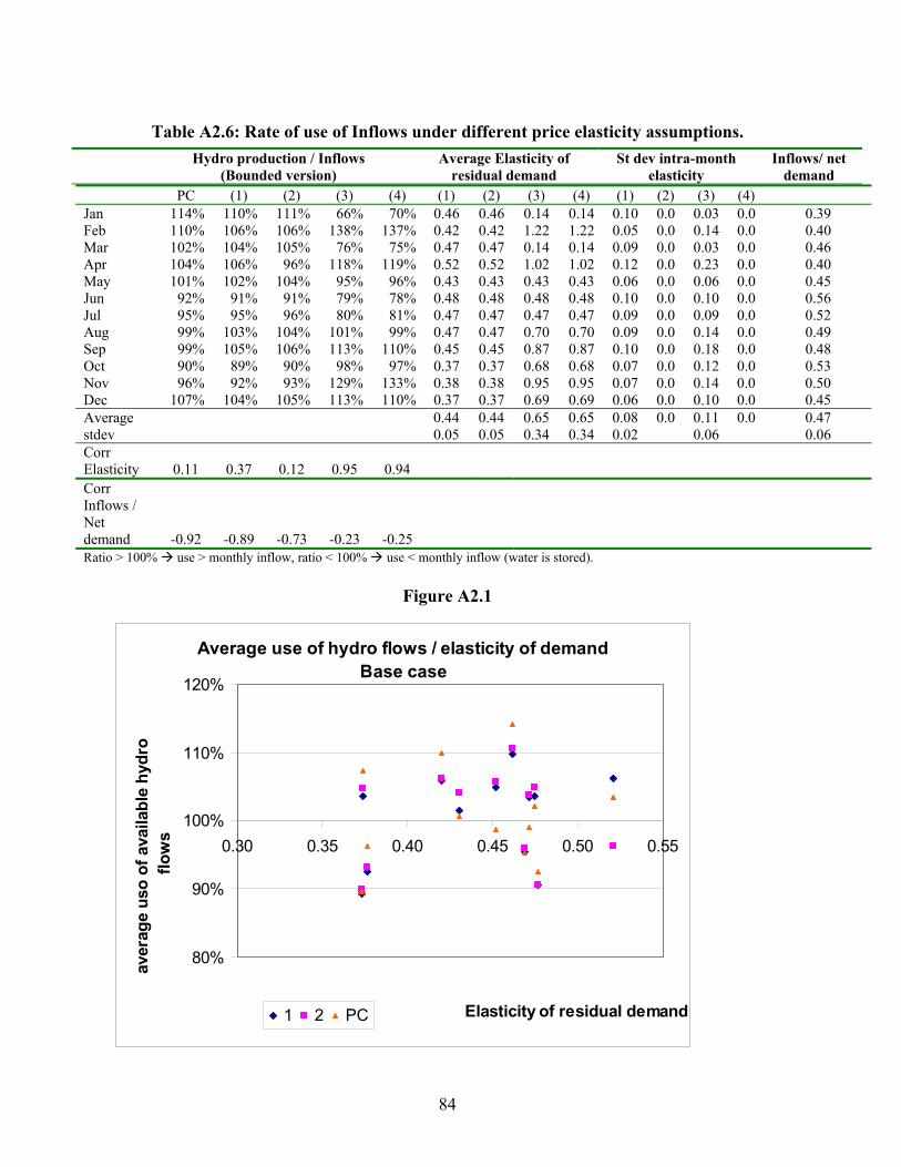
Table A2.6: Rate of use of Inflows under different price elasticity assumptions.

PC (1) (2) (3) (4) (1) (2) (3) (4) (1) (2) (3) (4) Jan 114% 110% 111% 66% 70% 0.46 0.46 0.14 0.14 0.10 0.0 0.03 0.0 0.39 Feb 110% 106% 106% 138% 137% 0.42 0.42 1.22 1.22 0.05 0.0 0.14 0.0 0.40 Mar 102% 104% 105% 76% 75% 0.47 0.47 0.14 0.14 0.09 0.0 0.03 0.0 0.46 Apr 104% 106% 96% 118% 119% 0.52 0.52 1.02 1.02 0.12 0.0 0.23 0.0 0.40 May 101% 102% 104% 95% 96% 0.43 0.43 0.43 0.43 0.06 0.0 0.06 0.0 0.45 Jun 92% 91% 91% 79% 78% 0.48 0.48 0.48 0.48 0.10 0.0 0.10 0.0 0.56 Jul 95% 95% 96% 80% 81% 0.47 0.47 0.47 0.47 0.09 0.0 0.09 0.0 0.52 Aug 99% 103% 104% 101% 99% 0.47 0.47 0.70 0.70 0.09 0.0 0.14 0.0 0.49 Sep 99% 105% 106% 113% 110% 0.45 0.45 0.87 0.87 0.10 0.0 0.18 0.0 0.48 Oct 90% 89% 90% 98% 97% 0.37 0.37 0.68 0.68 0.07 0.0 0.12 0.0 0.53 Nov 96% 92% 93% 129% 133% 0.38 0.38 0.95 0.95 0.07 0.0 0.14 0.0 0.50 Dec 107% 104% 105% 113% 110% 0.37 0.37 0.69 0.69 0.06 0.0 0.10 0.0 0.45 Average 0.44 0.44 0.65 0.65 0.08 0.0 0.11 0.0 0.47 stdev 0.05 0.05 0.34 0.34 0.02 0.06 0.06 Corr Elasticity 0.11 0.37 0.12 0.95 0.94 Corr Inflows / Net demand -0.92 -0.89 -0.73 -0.23 -0.25

Hydro production / Inflows (Bounded version)

Average Elasticity of residual demand

St dev intra-month elasticity

Inflows/ net demand

Ratio > 100% use > monthly inflow, ratio < 100% use < monthly inflow (water is stored).

Figure A2.1 Average use of hydro flows / elasticity of demand

Base case

80%

90%

100%

110%

120%

0.30 0.35 0.40 0.45 0.50 0.55

Elasticity of residual demand

aver

age

uso

of a

vaila

ble

hydr

o flo

ws

1 2 PC

84

Figure A2.2

Figure A2.3

Average use of hydro flows vs Inflows/ddandBase Case

80%

90%

100%

110%

120%

0.30 0.35 0.40 0.45 0.50 0.55 0.60

Inflows/demand

aver

age

uso

of a

vaila

ble

hydr

o flo

ws

1 2 PC

Figure A2.3

El

Average use of hydro flows / elasticity of demand(Larger inter-month difference)

60%

70%

80%

90%

100%

110%

120%

0.00 0.50 1.00 1.50

asticity of residual demand

aver

age

uso

of a

vaila

ble

hydr

o flo

ws

3 4 PC

85

86

Figure A2.4

Average use of hydro flows vs Inflows/ddand(Larger inter-month difference)

60%

70%

80%

90%

100%

110%

120%

0.30 0.35 0.40 0.45 0.50 0.55 0.60

Inflows/demand

aver

age

uso

of a

vaila

ble

hydr

o flo

ws

3 4 PC