diagnostic and treatment for linear mixed models
TRANSCRIPT

Diagnostic and treatment for linear mixed models
Julio M. Singer
in collaboration withFrancisco M.M. Rocha and Juvencio S. Nobre
Departamento de EstatısticaUniversidade de Sao Paulo, Brazil
www.ime.usp.br/∼jmsinger
JM Singer (USP) ICORS 2015, Kolkata, India 1 / 39

Ozone example
Ozone concentration: measured with expensive instrumentsAlternative: reflectance in passive filters / calibration curveDetails in Andre et al. (2014, Atm. Environ.)
JM Singer (USP) ICORS 2015, Kolkata, India 2 / 39

Ozone example
Experiment LPAE/FMUSP: predict period expected reflectance(latent value) accounting for possible outliers
Period Reflectance Period Reflectance1 27.0 6 47.91 34.0 6 60.41 17.4 6 47.32 24.8 7 50.42 29.9 7 50.72 32.1 7 55.93 35.4 8 54.93 63.2 8 43.23 27.4 8 52.14 51.2 9 38.84 54.5 9 59.94 52.2 9 61.15 77.75 53.95 48.2
JM Singer (USP) ICORS 2015, Kolkata, India 3 / 39

Ozone example
Linear mixed model:
yij = µ+ ai + eij , i = 1, . . . , 9, j = 1, 2, 3
ai ∼ N(0, σ2a) independent
eij ∼ N(0, σ2) independent
ai and eij independent
Consequently
V(yij) = σ2a + σ2
Cov(yij , yik) = σ2a
Cov(ylj , yik) = 0
Intraclass correlation coefficient: ρ = σ2a/(σ
2a + σ2)
JM Singer (USP) ICORS 2015, Kolkata, India 4 / 39

Gaussian LMM (matrix notation)
yi = Xiβ + Zibi + ei with V(bi) = G and V(ei) = Ri
so that
E(yi) = Xiβ and V(yi) = Ωi = ZiGZ>i + Ri
Ozone example
yi =
yi1yi2yi3
, Xi =
111
, β = µ, bi = ai, ei =
ei1ei2ei3
V(ai) = σ2a, V(eij) = σ2, Ωi =
σ2a + σ2 σ2a σ2aσ2a σ2a + σ2 σ2aσ2a σ2a σ2a + σ2
JM Singer (USP) ICORS 2015, Kolkata, India 5 / 39

Gaussian LMM (matrix notation)
y = Xβ + Zb + e
with
y = (y>1 , · · · ,y>n )> (N × 1, N =∑n
i=1mi)
X = (X>1 , · · · ,X>n )> (N × p)
Z = ⊕ni=1Zi (N × nq)
b = (b>1 , · · · ,b>n )> (nq × 1)
e = (e>1 , · · · , e>n )> (N × 1)
Γ = In ⊗G(θ) (nq × nq)
R = ⊕ni=1Ri(θ) (N ×N)
ConsequentlyV(y) = V = ZΓZ> + R
JM Singer (USP) ICORS 2015, Kolkata, India 6 / 39

Maximum likelihood methodology
(E)BLUE of β : β =(∑n
i=1 X>i Ω−1i Xi
)−1∑ni=1 X>i Ω
−1i yi
(E)BLUP of
bi : bi = GZ>i Ω−1i [Imi −Xi
(X>i Ω
−1i Xi
)−1X>i Ω
−1i ]yi
Ozone example
β = y, bi = k(yi − y), k = σ2a/(σ2a + σ2/3)
k: shrinkage constant
Predicted latent value for period i
yi = y + k(yi − y) = kyi + (1− k)y
JM Singer (USP) ICORS 2015, Kolkata, India 7 / 39

Diagnostics
Global influenceLeverage analysis [Nobre and Singer (2011, J. Applied Stat.)]Case deletion analysis [Tan et al. (2001, The Statistician)]
Local influence [Lesaffre and Verbeke (1998, Biometrics)]Residual analysis [Nobre and Singer (2007, Biom. Journal)]Three types of residuals to accommodate the extra source ofvariability present in LMM:
i) Marginal residuals, ξi = yi −Xiβ predictors of marginal errors,ξi = yi −E[yi] = yi −Xiβ = Zibi + ei
ξij = yij − y
ii) Conditional residuals, ei = yi −Xiβ − Zibi predictors of conditionalerrors ei = yi −E[yi|bi] = yi −Xiβ − Zibi
eij = yij − yi
iii) Random effects residuals, Zibi, predictors of random effects,Zibi = E[yi|bi]−E[yi] = (yi −Xiβ − Zibi)− (yi −Xiβ)
bij = yi − yJM Singer (USP) ICORS 2015, Kolkata, India 8 / 39

LMM Residual analysis
Standardized marginal residual: ξ∗ij = ξij/[diagij(V(ξi))]
1/2
V(ξi) = Ωi −Xi(XiΩ−1i Xi)
−1X>i
Standardized conditional residual: e∗ij = eij/[diagj(RiQiRi)]1/2
V(ei) = RiQiRi with Qi = Ω−1i −Ω
−1i Xi
(X>i Ω
−1i Xi
)−1X>i Ω
−1i
Modified Lesaffre-Verbeke index:
Vi = ||Imi − V(ξi)−1/2ξiξ
>i V(ξi)
−1/2||2, V∗i =√Vi/mi
Mahalanobis distance: Mi = b>i [V(bi − bi)]−1bi
JM Singer (USP) ICORS 2015, Kolkata, India 9 / 39

Confounding
e = RQe + RQZb
Hilden-Minton (1995, PhD thesis, UCLA): ability to check fornormality of e, using e, decreases as V[RQZ>b] = RQZGZ>QRincreases in relation to V[RQe] = RQRQR
Fraction of confounding for the k-th conditional residual ek
0 ≤ Fk =u>k RQZΓZ>QRuk
u>k RQRuk= 1−
u>k RQRQRuk
u>k RQRuk≤ 1
Least confounded residual: linear transformation c>e that minimizesFraction of Confounding
Least confounded residuals: homoskedastic, uncorrelated
Useful for constructing QQ plots to check for normality
JM Singer (USP) ICORS 2015, Kolkata, India 10 / 39

Residual diagnostics for Gaussian LMM
Diagnostic for Residual Plot
Linearity of effects fixed (E[y] = Xβ) Marginal ξ∗ij vs fitted values orexplanatory variables
Presence of outlying observations Marginal ξ∗ij vs observation indicesWithin-subjects covariance matrix (Vi) Marginal V∗i vs unit indicesPresence of outlying observations Conditional e∗ij vs observation indicesHomoskedasticity of conditional errors (ei) Conditional e∗ij vs predicted valuesNormality of conditional errors (ei) Conditional Normal QQ plot for c>k e
∗
Presence of outlying units Random effects Mi vs unit indicesNormality of the random effects (bi) Random effects χ2
q QQ plot for Mi
Diagnostic tools depend on correct specification of covariancestructure
JM Singer (USP) ICORS 2015, Kolkata, India 11 / 39

Post diagnostic treatment
Fine tuning of the model based on diagnostic toolsExamination of individual profiles [Rocha and Singer (2014), submitted]Plots of correlations vs lags [Grady and Helms (1995, SIM)]Use of covariates to model covariance structure [Curi and Singer(2006), Environ Ecol Stat]
Elliptically symmetric distributionsUseful to accommodate outliers (multivariate t, slash, contaminatednormal)Estimation similar but more complicated than gaussian caseLocal influence [Osorio et al. (2007, CSDA)]Residual analysis?
Skew-elliptical distributionsFitting is difficult in practice; usually must consider Bayesian methodsLocal influence [Jara et al. (2008, CSDA)]Residual analysis?
Robust estimation [Koller (2013), PhD thesis, ETH Zurich]M-methodsLimited choices for covariance structure
JM Singer (USP) ICORS 2015, Kolkata, India 12 / 39

Computation
Random effects G or RW Error RiLibrary Function Fits distribution matrix distribution matrix
lme4 lmer LMM gaussian unstructured G gaussian σ2Iminlmer NLMM gaussian unstructured G gaussian structuredglmer GLMM gaussian unstructured G exponential NA
familynlme lme LMM gaussian structured G gaussian structured
nlme NLMM gaussian structured G gaussian structuredgls LM NA NA gaussian structured
gee gee GEE-based NS structured RW exponential NAmodel family or NS
geepack geeglm GEE-based NS structured RW exponential NAmodel family or NS
heavy heavyLme ES-LMM elliptically unstructured G elliptically NAsymmetric symmetric
robustlmm rlmer Robust LMM symmetric diagonal or symmetric σ2Imiunstructured G
NA: not applicableNS: not specified
Some functions for diagnostic available only from authors
Difficult to use in more complicated problems
First version of functions for residual diagnostic based on lme4 and nlmeavailable from www.ime.usp.br/∼jmsinger/lmmdiagnostics.zip
JM Singer (USP) ICORS 2015, Kolkata, India 13 / 39

Ozone example - standard model (A)
Results (standard model): µ = 46.4, σ2a = 100.4, σ2 = 104.8, k = 0.75
Standardized marginal residuals - standard model
30 40 50 60
−3
−2
−1
01
23
Marginal fitted values
Sta
ndar
dize
d m
argi
nal r
esid
uals
1.3
5.1
Standardized marginal residuals
Den
sity
−4 −2 0 2 4
0.0
0.1
0.2
0.3
0.4
0.5
JM Singer (USP) ICORS 2015, Kolkata, India 14 / 39
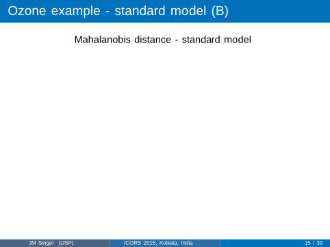
Ozone example - standard model (B)
Mahalanobis distance - standard model
2 4 6 8
01
23
45
67
Unit index
Mah
alan
obis
dis
tanc
e
1
2
JM Singer (USP) ICORS 2015, Kolkata, India 15 / 39

Ozone example standard model (C)
QQ plot for Mahalanobis distance - standard model
0.0 0.5 1.0 1.5 2.0 2.5 3.0
0.0
0.5
1.0
1.5
2.0
2.5
3.0
3.5
Chi−squared quantiles
Mah
alan
obis
dis
tanc
e
JM Singer (USP) ICORS 2015, Kolkata, India 16 / 39

Ozone example standard model (D)
Modified Lesaffre-Verbeke index - standard model
2 4 6 8
01
23
4
Unit index
Mod
ified
Les
affr
e−V
erbe
ke in
dex
3
JM Singer (USP) ICORS 2015, Kolkata, India 17 / 39

Ozone example - standard model (E)
Standardized conditional residuals - standard model
35 40 45 50 55
−3
−2
−1
01
23
Predicted values
Sta
ndar
dize
d co
nditi
onal
res
idua
ls
3.2 5.1
Standardized conditional residuals
Den
sity
−4 −2 0 2 4
0.0
0.1
0.2
0.3
0.4
JM Singer (USP) ICORS 2015, Kolkata, India 18 / 39

Ozone example - standard model (F)
Standardized least confounded conditional residuals - standardmodel
−2 −1 0 1 2
−1
01
2
N(0,1) quantiles
Sta
ndar
dize
d le
ast c
onfo
unde
d re
sidu
als
Standardized least confounded residuals
Den
sity
−4 −2 0 2 4
0.00
0.05
0.10
0.15
0.20
0.25
0.30
JM Singer (USP) ICORS 2015, Kolkata, India 19 / 39

Ozone example - heteroskedastic model 1 (A)
Suggested (heteroskedastic) model
yij = µ+ ai + eij with eij ∼ N(0, σ2i )
For parsimony: σ2i = τ2, i = 3, 5, σ2i = σ2, otherwise
Shrinkage constant: ki = σ2a/(σ2a + σ2i /3)
Predicted latent value for period i
yi = µ+ ki(yi − µ), µ =
9∑i=1
(wi/
9∑i=1
wi)yi, wi = (σ2a + σ2i )−1
Results
Heteroskedastic model 1: µ = 45.9, σ2a = 114.3, σ2 = 49.6,τ2 = 274.0, ki 6=3,5 = 0.87, ki=3,5 = 0.56
Homoskedastic model: µ = 46.4, σ2a = 100.4, σ2 = 104.8,k = 0.75
JM Singer (USP) ICORS 2015, Kolkata, India 20 / 39

Ozone example - heteroskedastic model 1 (B)
Modified Lesaffre-Verbeke index - heteroskedastic model 1
2 4 6 8
01
23
4
Unit index
Mod
ified
Les
affr
e−V
erbe
ke in
dex
9
JM Singer (USP) ICORS 2015, Kolkata, India 21 / 39
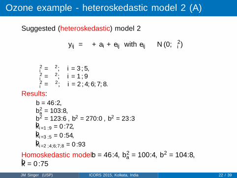
Ozone example - heteroskedastic model 2 (A)
Suggested (heteroskedastic) model 2
yij = µ+ ai + eij with eij ∼ N(0, σ2i )
σ2i = τ2, i = 3, 5,σ2i = ν2, i = 1, 9σ2i = σ2, i = 2, 4, 6, 7, 8.
Results:
µ = 46.2,σ2a = 103.8,σ2 = 123.6 , τ2 = 270.0 , ν2 = 23.3ki=1,9 = 0.72,
ki=3,5 = 0.54,
ki=2,4,6,7,8 = 0.93
Homoskedastic model: µ = 46.4, σ2a = 100.4, σ2 = 104.8,k = 0.75
JM Singer (USP) ICORS 2015, Kolkata, India 22 / 39

Ozone example heteroskedastic model 2 (B)
Standardized conditional residuals - heteroskedastic model 2
35 40 45 50
−3
−2
−1
01
23
Predicted values
Sta
ndar
dize
d co
nditi
onal
res
idua
ls
9.1
Standardized conditional residuals
Den
sity
−4 −2 0 2 4
0.0
0.1
0.2
0.3
JM Singer (USP) ICORS 2015, Kolkata, India 23 / 39

Ozone example - heteroskedastic model 2 (C)
Standardized least confounded conditional residuals -heteroskedastic model 2
−2 −1 0 1 2
−2
−1
01
2
N(0,1) quantiles
Sta
ndar
dize
d le
ast c
onfo
unde
d re
sidu
als
Standardized least confounded residuals
Den
sity
−4 −2 0 2 4
0.0
0.1
0.2
0.3
0.4
JM Singer (USP) ICORS 2015, Kolkata, India 24 / 39

Ozone example - data revisited
Period Reflectance Period Reflectance
1 27.0 6 47.91 34.0 6 60.41 17.4 6 47.32 24.8 7 50.42 29.9 7 50.72 32.1 7 55.93 35.4 8 54.93 63.2 8 43.23 27.4 8 52.14 51.2 9 38.84 54.5 9 59.94 52.2 9 61.15 77.75 53.95 48.2
JM Singer (USP) ICORS 2015, Kolkata, India 25 / 39

Ozone example – Latent value predictions
Sample Homoskedastic HeteroskedasticPeriod mean LMM LMM (3 variances) t (df=21.8) Robust
1 26.1 31.4 31.9 31.8 29.22 28.9 33.4 30.2 33.8 31.63 42.0 43.1 44.0 43.3 39.44 52.6 51.0 52.2 50.9 51.55 59.9 56.4 53.5 56.3 54.46 51.9 50.4 51.5 50.4 50.97 52.3 50.8 51.9 50.8 51.38 50.1 49.1 49.8 49.1 49.49 53.3 51.5 51.3 51.4 52.7
Mean 46.4 46.4 46.2 46.6 45.7
Shrinkage towards mean (sample mean-latent value prediction)Homoskedastic Heteroskedastic
Period LMM LMM (3 variances) t(df=21.8) Robust3 -1.1 -2.0 -1.3 2.65 3.5 6.4 3.6 5.5
JM Singer (USP) ICORS 2015, Kolkata, India 26 / 39

Boston house price example
Data originally from Harrison and Rubinfeld (1978, J Environ Econ &Manag)
Used as example of heavy-tailed data Belsley et al. (1980, Wiley),Longford (1993, Oxford)
Objective: Willingness to pay for better air quality based on theanalysis of housing market
Data on 14 variables obtained from 506 SMSA arising form 92 towns
Belsley et al. (1980) fitted standard linear model via OLS
yi = explanatory variables + ei, ei ∼ N(0, σ2)
i = 1, . . . , 506 and suggested that error distribution should haveheavier tails than the gaussian distribution
JM Singer (USP) ICORS 2015, Kolkata, India 27 / 39

Boston example: Belsley et al. model
Standardized conditional residuals - Belsley et al. model
−3 −2 −1 0 1 2 3
−4
−2
02
4
N(0,1) quantiles
Sta
ndar
dize
d m
argi
nal r
esid
uals
JM Singer (USP) ICORS 2015, Kolkata, India 28 / 39
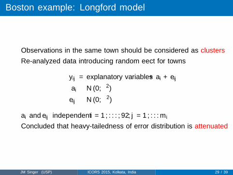
Boston example: Longford model
Observations in the same town should be considered as clusters
Re-analyzed data introducing random effect for towns
yij = explanatory variables + ai + eij
ai ∼ N(0, τ2)
eij ∼ N(0, σ2)
ai and eij independent i = 1, . . . , 92, j = 1, . . .mi
Concluded that heavy-tailedness of error distribution is attenuated
JM Singer (USP) ICORS 2015, Kolkata, India 29 / 39
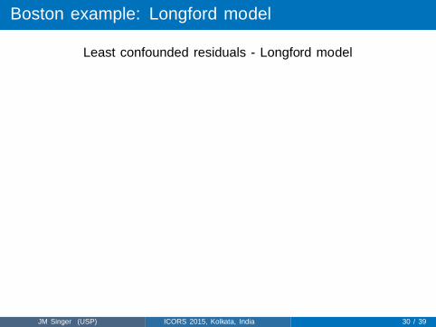
Boston example: Longford model
Least confounded residuals - Longford model
−3 −2 −1 0 1 2 3
−4
−3
−2
−1
01
23
N(0,1) quantiles
Sta
ndar
dize
d le
ast c
onfo
unde
d re
sidu
als
Standardized least confounded residuals
Den
sity
−6 −4 −2 0 2 4 6
0.0
0.1
0.2
0.3
JM Singer (USP) ICORS 2015, Kolkata, India 30 / 39

Boston example: Longford model
QQ plot for Mahalanobis distance - Longford model
0 2 4 6 8
05
1015
20
Chi−squared quantiles
Mah
alan
obis
dis
tanc
e
JM Singer (USP) ICORS 2015, Kolkata, India 31 / 39
Boston example: Longford model diagnostics
Modified Lesaffre-Verbeke index - Longford model
0 20 40 60 80
05
1015
20
Unit index
Mod
ified
Les
affr
e−V
erbe
ke in
dex
7677
80
81
8283
90
92
JM Singer (USP) ICORS 2015, Kolkata, India 32 / 39

Boston example: final model
Diagnostics re-examined after fitting alternative models
Final model
yij = explanatory variables + ai + eij
ai ∼ N(0, τ2)
ei ∼ Nmi(0,Ri), Ri compound symmetry
Ri = R∗i , i = 4, 15, . . . , 91, 92 : selected towns
Ri = R∗, otherwise
ai and ei independent i = 1, . . . , 92, j = 1, . . .mi
Compound symmetry to allow for possible within-unit spatialcorrelation
Different within-unit covariance matrix for selected SMSAs
JM Singer (USP) ICORS 2015, Kolkata, India 33 / 39

Boston example: final model
Standardized marginal residuals - final model
9.0 9.5 10.0 10.5
−4
−2
02
4
Marginal fitted values
Sta
ndar
dize
d m
argi
nal r
esid
uals
3.230.1
31.331.639.3
39.539.10
42.342.6
46.5
57.158.1
75.7
79.781.781.8
85.11
Standardized marginal residuals
Den
sity
−6 −4 −2 0 2 4 6
0.00
0.10
0.20
0.30
JM Singer (USP) ICORS 2015, Kolkata, India 34 / 39

Boston example: final model
Mahalanobis distance - final model
0 20 40 60 80
02
46
810
Unit index
Mah
alan
obis
dis
tanc
e
3
1631
3942
4546
57
6263
7577
79
81 86
JM Singer (USP) ICORS 2015, Kolkata, India 35 / 39

Boston example: final model
QQ plot for Mahalanobis distance - final model
0 2 4 6 8
01
23
45
Chi−squared quantiles
Mah
alan
obis
dis
tanc
e
JM Singer (USP) ICORS 2015, Kolkata, India 36 / 39

Boston example: final model
Standardized conditional residuals - final model
9.0 9.5 10.0 10.5
−4
−2
02
4
Predicted values
Sta
ndar
dize
d co
nditi
onal
res
idua
ls
3.230.1
31.331.639.3
39.539.10
42.342.6
46.5
57.158.1
75.7
79.781.781.8
85.11
Standardized conditional residuals
Den
sity
−6 −4 −2 0 2 4 6
0.00
0.10
0.20
0.30
JM Singer (USP) ICORS 2015, Kolkata, India 37 / 39

Boston example: final model
Least confounded residuals - final model
−3 −2 −1 0 1 2 3
−3
−2
−1
01
23
N(0,1) quantiles
Sta
ndar
dize
d le
ast c
onfo
unde
d re
sidu
als
Standardized least confounded residuals
Den
sity
−6 −4 −2 0 2 4 6
0.0
0.1
0.2
0.3
JM Singer (USP) ICORS 2015, Kolkata, India 38 / 39

Boston example: estimates of fixed effects
Gaussian LMM t -LMM RobustBelsley Longford Final df=2.19 LMM
Var Estim SE Estim SE Estim SE Estim SE Estim SE(Int) 9.756 0.150 9.672 0.214 9.669 0.125 9.682 0.250 9.612 0.158crim -0.012 0.001 -0.007 0.001 -0.006 0.002 -0.006 0.002 -0.006 0.001zn 0.000 0.001 0.000 0.001 0.000 0.000 0.001 0.001 0.001 0.001indus 0.000 0.002 0.002 0.005 0.003 0.003 0.003 0.006 0.004 0.003chasyes 0.091 0.033 -0.014 0.029 0.017 0.018 0.016 0.042 -0.004 0.022nox -0.006 0.001 -0.006 0.001 -0.005 0.001 -0.005 0.003 -0.005 0.001rm 0.006 0.001 0.009 0.001 0.018 0.001 0.018 0.002 0.014 0.001age 0.000 0.001 -0.001 0.001 -0.002 0.000 -0.002 0.001 -0.002 0.000dis -0.191 0.033 -0.125 0.047 -0.116 0.029 -0.117 0.058 -0.109 0.035rad 0.096 0.019 0.098 0.030 0.062 0.018 0.073 0.027 0.078 0.022tax -0.000 0.000 -0.000 0.000 -0.000 0.000 -0.000 0.000 -0.000 0.000ptratio -0.031 0.005 -0.030 0.010 -0.024 0.006 -0.025 0.011 -0.026 0.008blacks 0.364 0.103 0.582 0.101 0.657 0.088 0.639 0.186 0.659 0.076lstat -0.371 0.025 -0.282 0.024 -0.113 0.016 -0.099 0.032 -0.195 0.018
JM Singer (USP) ICORS 2015, Kolkata, India 39 / 39