diagnostic verification of atmospheric water cycle ...€¦ · diagnostic verification of...
TRANSCRIPT

Diagnostic Verification of Atmospheric Water
Cycle Predicted by Regional Mesoscale Models and Ensemble Systems
Dissertation zur Erlangung des Doktorgrades
der Naturwissenschaften im Department Geowissenschaften
der Universität Hamburg
vorgelegt von
Suraj Devidasrao Polade aus
Dawargaon, Indien
Hamburg 2012

Als Dissertation angenommen vom Department Geowissenschaften der Universität Hamburg auf Grund der Gutachten von Prof. Dr. Felix Ament und Prof. Dr. Susanne Crewell Hamburg, den 25. Januar 2012 Professor Dr. Jürgen Oßenbrügge (Leiter des Department Geowissenschaften)

i
Acknowledgements
I would like to express my profound gratitude towards my supervisors Felix Ament and
Susanne Crewell for their valuable time and discussions during the course. Their enthusiasm,
optimism and encouraging remarks throughout the project kept me motivated and made for
an enjoyable period of research. I am also grateful to Marco Clemens for his discussions. I
would like to acknowledge Axel Seifert for his comments and discussions during the QUEST
project, which was very helpful for this study. I would like to thank all QUEST members for
their lively discussions. Mark Carson is greatly acknowledged for proofreading my disserta-
tion and providing me valuable comments. I also would like to thank my colleagues Kathari-
na Lengfeld, Nicole Feiertag, Sarah Sandoval, and Seshagirirao Kolusu for their friendship
and help during the course. I express by special thanks to C. Seethala, who provided constant
moral support whenever I was in need. I would like to thank my parents and siblings for their
encouragement.
Hamburg, 25.01.2012 Suraj Polade

ii
iii
Abstract
Precipitation is the final component of a complex process chain of the atmospheric water
cycle. All model errors in this process chain are consequently accumulated in quantitative
precipitation forecasts (QPF). To diagnose the shortcomings of QPF, the following four key
variables of the atmospheric water cycle have been evaluated: integrated water vapour
content (IWV), low cloud cover (LCC), high cloud cover (HCC), and precipitation rate at the
surface. This comprehensive verification of all key variables is performed for nine
deterministic models and four ensemble systems from the forecast demonstration experiment
of Mesoscale Alpine Program (MAP D-PHASE) using measurements from the General
Observation Period (GOP) over Southern Germany for summer 2007. Verification of
individual key variables reveals that most of the models forecast the mean values of IWV
very well; however, they show large biases in the mean values of LCC, HCC, and
precipitation. At certain times and locations, all models show large errors in all key variables,
especially in HCC and precipitation. The models with convection parameterization predict
diurnal precipitation maxima a few hours earlier than observations, whereas deep-convection-
resolving models forecast the diurnal maxima too late. Early initiation of convection is a
specific problem of the Tiedtke convection scheme. The forecast performance of high
resolution models is superior to their corresponding low resolution models for all key
variables, except for IWV. Multivariate verification fails to quantify the shortcomings in
QPF, perhaps due to the limited availability of observations. Multimodel multiboundary
ensemble prediction systems (EPS) show superiority in the prediction of all key variables and
also has better representation of forecast uncertainty compared to EPS based on a single
model. EPS which accounts the small-scale perturbations, due to the uncertainty in boundary
and initial conditions from limited area models, lead to better forecasts for strong events.
However, all the EPS evaluated in this study are underdispersive which clearly implies that
they are not able to account for all possible uncertainties of short-range forecasts.

iv

v
Zusammenfassung
Die genaue Prognose der quantitativen Niederschlagsvorhersage (QPF, engl. quantitative
precipitation forecast) ist eine der schwierigsten Aufgaben, die noch nicht befriedigend in der
numerischen Wettervorhersage umgesetzt wurde. Da der Niederschlag das letzte Glied einer
komplexen Kette von Prozessen des atmosphärischen Wasserkreislaufs darstellt,
akkumulieren sich alle Modellfehler dieser Prozesskette in der quantitativen
Niederschlagsvorhersage. Um die Defizite der QPF zu untersuchen, haben wir den
kompletten atmosphärischen Wasserkreislauf beginnend mit dem integrierten
Wasserdampfgehalt (IWV, engl. integrated water vapor content) über die Bewölkung bis hin
zur Niederschlagsmenge an der Oberfläche ausgewertet. Eine umfassende Verifizierung des
atmosphärischen Wasserkreislaufs wurde für neun deterministische Modelle und vier
Ensembles des MAP D-PHASE Experiments, welches GOP Beobachtungen über
Süddeutschland vom Sommer 2007 einbezieht, durchgeführt. Die Überprüfung der
wichtigsten Größen zeigt, dass der IWV und der Bedeckungsgrad der tiefen Wolken (LCC,
engl. low cloud cover) sehr gut von den meisten Modellen vorhergesagt werden. Jedoch
treten große Abweichungen in der hohen Bewölkung (HCC, engl. high cloud cover) und der
Niederschlagprognose auf, deren hauptsächliche Ursache in den Schwächen des
Mikrophysikschemas und der ungenauen Behandlung der Konvektion in den Modellen liegt.
Außerdem zeigen alle Modelle große Fehler zu bestimmten Zeiten und Orten oder
Gitterzellen, im Vergleich zu den systematischen Fehlern der wichtigsten Größen. Dies zeigt
sich besonders in dem HCC und dem Niederschlag.
Modelle mit Konvektionsparametrisierung sagen das tägliche Niederschlagsmaximum zu
früh vorher, wobei Modelle, die Konvektion explizit auflösen, das tägliche Maximum zu spät
vorhersagen. Die verfrühte Vorhersage ist insbesondere ein Problem des Tiedke-
Konvektionsschemas. Die Qualität der Vorhersagen von hochauflösenden Modellen gegen-
über niedrigauflösenden Modellen ist für alle Schlüsselvariablen besser, jedoch nicht für den
IWV. Die Defizite der QPF können auch nicht durch multivariate Analysen quantifiziert
werden, möglicherweise aufgrund unzureichender Beobachtungsdaten. Das Multi-Models
Multi-Boundary Ensemble-Vorhersage-System (engl. ensemble prediction system, EPS) ist
für die Vorhersage aller Schlüsselvariablen besser geeignet. Desweiteren ist es den EPS-
basierten Einzelmodellen bei der Darstellung der Vorhersageunsicherheit überlegen. EPS
führt zu besseren Vorhersagen von starke Ereignissen, da es aufgrund von Unsicherheiten in

vi
Rand- und Anfangsbedingungen der Regionalmodelle kleinskalige Störungen berücksichtigt.
Dennoch zeigen alle in dieser Studie untersuchten EPS zu wenig Streuung, was eindeutig
zeigt, dass sie nicht in der Lage sind alle möglichen Unsicherheiten der kurzfristigen Vorher-
sage zu berücksichtigen.
vii
Contents
Acknowledgements
i
Abstract
iii
Zusammenfassung
v
List of Abbreviations
ix
1 Introduction and Motivation 1
1.1 Review of Representation of Atmospheric Water Cycle in Numerical
Models…………………………………………………………………
2
1.2 Different Verification Strategies …………………………………….... 5
1.3 Thesis Aims ……………………………………………………………. 7
2 Data and Methodology 9
2.1 Observations …………………………………………………………… 9
2.1.1 GPS Network to Observe IWV…………………………………... 10
2.1.2 Ceilometer Network to Observe LCC ……………………….….. 11
2.1.3 MSG based Retrieval of HCC …………………………….…….. 12
2.1.4 Gauge and Radar based Precipitation Estimate …………………. 13
2.2 Model Description ……………………………………………………... 15
2.3 Ensemble Forecasting …………………………………………………. 20
2.3.1 Introduction to Ensemble Forecasting ………………………….. 20
2.3.2 Description of Ensemble Systems ………………………………. 21
2.4 Comparison of Models grid-cell with Station Observations …….….… 24
2.5 Verifications Methodology ……………………………………….…... 25
2.6 Concept of Most-recent and 0000 UTC run Forecast …………………. 29
3 Evaluation of Integrated Water Vapor, Cloud Cover and Precipitation
Predicted by Mesoscale Models
31
3.1 Spatial and Temporal Averaged Verification …..……………….…….. 31
3.2 Verification of Mean Diurnal Variability ……………………..………. 34
3.2.1 Integrated Water Vapour ………………………………….…….. 34
3.2.2 Low Cloud Cover ……………………………………….……….. 36

viii
3.2.3 High Cloud Cover ………………………………………………. 38
3.2.4 Precipitation …………………………………………..………… 39
3.3 Spatial Distributions in Model Simulations …………………………... 42
3.3.1 Integrated Water Vapour ……………………………………….. 42
3.3.2 Low Cloud Cover ……………………………………………….. 43
3.3.3 High Cloud Cover ………………………………………………. 46
3.3.4 Precipitation ………………………………………………..…… 48
3.4 Verification of Models Skill with Forecast Length …………………… 51
4 Multivariate Multi-model Verification 53
4.1 Similarities among Variables ………………………….………….. 53
4.2 Similarities between Errors of Different Key Variables …………... 61
4.3 Similarities between Different Key Variables …………………….. 64
4.4 Similarities between Different Key Variables for Different Lag-
times ………………………………………………………………..
67
5 Evaluation of Integrated Water Vapor, Cloud Cover and Precipitation
Predicted by Ensemble Systems
71
5.1 Performance of Individual Ensemble Members and Ensemble Mean
Forecast …………………………………………………….
71
5.2 Representation of Forecast Uncertainty – An Assessment ………... 75
5.3 Assessment of Probabilistic Forecast Skill ………………………... 82
5.3.1 EPS Forecast Skill for Specific Events ……………………… 83
5.3.2 Global Skill of EPS’………………………………………….. 91
5.4 Summary …………………………………………………………... 92
6 Conclusions and Outlook 95
6.1 Summary and Conclusions ………………………………………… 95
6.2 Scope of Future Research ………………………………………… 101
References 103
Appendix A 121
Appendix B 135

ix
List of Abbreviations
3D-Var 3-Dimensional VARiational data assimilation
4D-Var 4-Dimensional VARiational data assimilation
ACSBTE Assumed Clear Sky Brightness Temperature
ALADIN Aire Limitée Adaptation dynamique Développement International
AROME Application of Research to Operational at Mesoscale
ARPA-SIM Regional Hydro-Meteorological Service of Emilia-Romagna, Italy
ARPEGE Action de Recherche Petite Echelle Grande Echelle (i.e. Research
Project on Small and Large Scales)
B01 Bechtold et al. [2001] convection parameterization scheme
BIAS Bias
BS Brier score
BSS Brier skill score
C00 Cuxart et al. [2000] turbulence is parameterization
CAPE Convective Available Potential Energy
CD01 Chen and Dudhia [2001] surface scheme
CM Cloud Mask
CNMCA National Meteorological Center, Italy
COPS Convective and Orographically-induced Precipitation Study
COSMO COnsortium for Small-scale MOdeling
COSMO-LEPS COnsortium for Small-scale MOdeling-Limited-area Ensemble
Prediction System
CPDF Complete Probability Distribution function
CRPS Continuous Ranked Probability Score
COSMO-SREPS COnsortium for Small-scale MOdeling- Short Range Ensemble
Prediction System
CTP Cloud Top Pressure
D07M Doms et al. [2007] microphysics scheme
D07T Doms et al. [2007] turbulence is parameterization scheme
DIST Distribution Method
D-PHASE Demonstration of Probabilistic Hydrological and Atmospheric
Simulation of flood Event in the Alpine region
DWD The German Meteorological Service

x
ECMWF European Centre for Medium-range Weather Forecasts
EPS Ensemble Prediction System
ESA European Space Agency
ETS Equitable Threat Score
EUMETSAT European Organization for the Exploitation of Meteorological
Satellites
FAR False Alarm Rate
FBIAS Frequency Bias
FUB Institute for Space Sciences at the Free University of Berlin,
Germany
FZK IMK-IFU Institute for Meteorology and Climate Research, Atmospheric
Environmental Research Division, Karlsruhe Institute of Technol-
ogy, Germany
G94 Grell et al. [1994] convection parameterization scheme
GFS Global Forecast System
GFZ German Research Centre for Geosciences
GME Global Mode
GOP General Observation Period
GPS Global Positioning System
H06 Heise et al. [2006] surface scheme
HCC High Cloud Cover
HIGHRES High Resolution
HP96 Hong and Pan [1996] turbulence is parameterization
HR Hit Rate
IFS Integrated Forecast System
INM Spanish Met Service
IWV Integrated Water Vapor content
LAM Limited Area Model
LAMEPSAT Limited Area Model Ensemble Prediction System Austria
LCC Low Cloud Cover
LIDAR Light Detection And Ranging
LOWRES Low Resolution
MAP Mesoscale Alpine Programme

xi
MSG Meteosat Second Generation
NCEP National Centers for Environmental Prediction
NOAA GFS National Oceanic and Atmospheric Administration Global Fore-
cast System
NP89 Noilhan and Planton [1989] surface scheme
NWP Numerical Weather Prediction
PDF Probability Distribution Function
PEPS Poor Man Ensemble System
PJ98 Pinty and Jabouille [1998] microphysics scheme
PQP German Priority Program on Quantitative Precipitation Forecast-
ing
QPF Quantitative Precipitation Forecast
R98 Reisner et al. [1998] microphysics scheme
RMSE Root Mean Squared Error
ROC Relative Operating Characteristic
ROCSS Relative Operating Characteristic Skill Score
SEVIRI The Spinning Enhanced Visible and InfraRed Imager
SRES Short Range Ensemble Forecasting Systems
STD Standard Deviation
T89 Tiedtke [1989] convection parameterization scheme
TDRE Trend Per Day in Random Error
TKE Turbulence Kinetic Energy
UM Global Unified Model
UTC Coordinated Universal Time
WWRP World Weather Research Programme
ZAMG Austrian Meteorological Service
ZHD Zenith Hydrostatic Delay
ZTD Zenith Total Delay
ZWD Zenith Wet Delay

xii
1
Chapter 1
Introduction and Motivation
Quantitative precipitation forecast (QPF) is one of the most challenging tasks of
weather prediction, which has not yet been satisfactorily resolved in the numerical weather
prediction (NWP) models [Ebert et al., 2003; Fritsch and Carbone, 2004]. Furthermore,
Hense et al. [2006] reported that in the last decades, no significant improvements have been
made in the skill of precipitation forecasts. However, accurate prediction of precipitation is
crucial for flood warning, daily weather forecasting, hydrological modeling, agriculture
purposes, etc.
The formation of precipitation involves different stages starting from water vapour. At
first, evaporation transports water vapour from the surface to the atmosphere. The atmospher-
ic instability causes air to rise further up in the atmosphere. At the point of saturation, the air
condenses and forms clouds. The hydrometeors inside the clouds grow by collision, coales-
cence, freezing and deposition and finally, fall out as precipitation. Since precipitation is the
final product of the atmospheric water cycle, errors in the representation of any of these
processes in the models would lead to inaccurate QPF. Precipitation formation processes
range from large-scale synoptic-lifting on a scale of ~1000 km to formation of cloud droplets
on micrometer scale. Most of these processes occur on a scale smaller than the model grid-
cell, and thus can not be resolved explicitly by NWP models; such small scale processes are
called as subgrid-scale processes. These subgrid-scale fluxes of heat, mass and moisture have
considerable impact on the grid-scale flow and thus their aggregate effects are accounted for
in the models by means of statistical approximations of grid-scale variables. The method of
accounting for statistical influence of the unresolved subgrid processes in the model with
respect to grid scale variables, by approximating the end effects without directly forecasting
them, is called parameterization. These approximations used in the parameterization of
precipitation formation processes lead to inaccurate QPF. Predictability of precipitation also
depends upon the lateral boundary and initial conditions. Uncertainty exists in initial and
boundary conditions due to the approximated observational basis. Hohenegger et al. [2006]
have shown that uncertainties in initial and boundary conditions grow very rapidly over the
whole model domain due to the non-linear dynamics.
Along with the imperfect parameterization of precipitation formation processes and
uncertainties in the initial and the boundary conditions, the non-linear interactions among

2 Introduction and Motivation
these processes are another limitation for prediction of the timing and intensity of precipita-
tion. Vannitsem [2006] reveals that the initial error due to the imperfect initial conditions
further deteriorates by the imperfect parameterization. Thus accurate prediction of precipita-
tion is not achievable by deterministic models even if they are able to resolve all processes
involved in the precipitation formation along with the quite accurate initial conditions, due to
their non-linear interactions among the precipitation formation processes. However, the
uncertainties arising due to imperfect initial conditions, and parameterization can be account-
ed for by the ensemble approach. Ensemble forecasting aims to incorporate all possible
uncertainty sources in a modeling system in terms of perturbations. The ensemble forecast
consists of multiple model runs initiated with the different perturbations.
Thus, as outlined above, the error arises in any process of atmospheric water cycle
due to the imperfect observation and parameterization leads to inaccurate precipitation
forecast. Hence, the main objective of this study is to validate the complete atmospheric
water cycle in mesoscale models to quantify the errors in this complex process chain. This
chapter aims at understanding and discussing the basis of representation of atmospheric water
cycle processes in current numerical models. A brief overview of different parameterization
schemes to represent the atmospheric water cycle and their limitations along with their
influence on the precipitation forecast are given in the first section. Different verification
strategies used in the literature to diagnose the models’ limitations are discussed in the second
section. The motivation and aim of this dissertation is provided at the end.
1.1 Review of Representation of Atmospheric Water Cycle in Numerical Models
As discussed, the fallout of hydrometeors from the clouds as precipitation starts by
condensation and growth of the hydrometeors. As the formation of hydrometeors occurs on
the micrometer scale, this process can not be resolved by NWP models. Thus, these micro-
physical processes are parameterized in the NWP models, in order to account the aggregate
effect of hydrometeor formation. The microphysical schemes emulate the processes by which
moisture is removed from the air, based on grid scale variables, and accounts for clouds and
precipitation. Microphysical schemes in numerical models can be categorized into bin and
bulk schemes. In the bin microphysics scheme, the total distribution of hydrometeors is
divided into a finite number of bin sizes. While in the bulk scheme, an analytic form of size
distribution is assumed for a few categories of hydrometeors. Most of the operational
mesoscale models use bulk microphysics schemes [Kessler, 1969; Kong and Yau, 1997] to
parameterize the effects of cloud microphysical processes. However bin microphysical

3 Introduction and Motivation
schemes are used in research models [Khain et al., 2004], especially in high-resolution cloud-
resolving models. This scheme can further be characterized into one or more moment
schemes: one moment scheme predicts only the mixing ratio for each species [e.g., Kessler,
1969; Kong and Yau, 1997], while in two-moment schemes, along with the mixing ratio, the
total number concentration of at least one species can be predicted [e.g., Ziegler, 1985;
Reisner et al., 1998; Seifert and Beheng, 2001]. Two-moment schemes provide greater
flexibility in representing the evolution of particle size distribution and thus improve the
microphysical processes. The type of hydrometeors and their characteristics considered in the
microphysical scheme greatly influence the precipitation distribution. Gilmore et al. [2004]
have shown that the inclusion of fast-falling graupel/hail species resulted in a larger amount
of accumulated precipitation. The increase of ground precipitation is also observed by
Reinhardt and Seifert [2006] by setting graupel/hail weighted towards large hail. Stein et al.
[2000] demonstrated that the importance of sophisticated cloud microphysics increases with
increasing model resolution, while Serafin and Ferretti [2007] claim that the microphysics
scheme does not have a significant impact on the precipitation forecast of coarse resolution
(convection parameterized) models.
Microphysical schemes require saturation of the air to form the hydrometeors, and
saturation can be attained by lifting of the air parcel. However, the rising of moist air and the
saturation can occur by different methods, such as large-scale ascent of moist air, convection
caused by the near surface heating of the moist air, moist air convergence, and orographic
lifting. Most of this lifting process can be resolved by mesoscale models, except convective
lifting. Convective lifting of the moist air occurs on scales which can not be resolved by the
mesoscale models. Thus, the end effect of subgrid-scale convection is parameterized in these
models. Convection schemes calculate the collective effects of an ensemble of convective
clouds in a model column as a function of grid-scale variables. They also redistribute heat,
and remove and redistribute moisture, producing clouds and precipitation. The end effect of
the subgrid-scale convection is accounted for by the convection parameterization in three
stages, first by determining the occurrence and the localization of convection (Trigger
function), secondly by determining the intensity of convection (closure), and finally by
determining the vertical distribution of heating, moistening and momentum changes. The
convection parameterization schemes can be categorized into three classes: schemes based on
moisture budgets [Kuo, 1965 and 1974], adjustment schemes [Manabe et al., 1965; Betts and
Miller, 1986] and Mass flux schemes [Arakawa and Schubert, 1974; Bougeault, 1985;
Tiedtke, 1989; Kain and Fritsch, 1990; Bechtold et al., 2001]. As most of the current

4 Introduction and Motivation
mesoscale models use convection parameterizations based on the bulk mass flux approach,
we intend to discuss the details of only this approach. In bulk mass flux schemes, the model
atmosphere is forced towards the convectively adjusted state when they are activated by the
mass exchange between clouds and the environment. Several studies revealed the limitation
of convection schemes for prediction of precipitation in convection-parameterized models
(hereafter coarse resolution models). Betts and Jakob [2002] and Guichard et al. [2004] have
shown that, in coarse resolution models, the maximum convective precipitation occur a
couple of hours earlier to that in the observations. Ebert et al. [2003] pointed out the frequent
occurrence of weak precipitation in coarse resolution models. Wulfmeyer et al. [2008] found
that the wind-ward/lee effect in coarse resolution models is characterized by too much rain
over the windward slope and over the crest of the mountain, and too little rain over leeward
side. Models with horizontal resolution smaller than 4 km can partially resolve the convection
(deep convection) and thus convection can be explicitly calculated, however, resolution
requirement for explicit calculation of convection is still questionable [Weisman et al., 2008;
Kain et al., 2008; Schwartz et al., 2009]. Studies by Clark et al. [2007] and Lean et al. [2008]
have shown deep-convection-resolving models (high resolution models) are better at repre-
senting the precipitation diurnal variability than coarse resolution models. Roberts and Lean
[2008] also found an improvement in heavy and highly localized precipitation forecasts by
high resolution models. However, high resolution models also suffer from limitations such as
explicit convection requiring grid-scale saturation, which leads to spurious delays in the onset
and subsequent over-prediction of convection [e.g., Kato and Saito, 1995; Kain et al., 2008].
Turbulent motion provides moisture to upward rising air. This turbulent motion oc-
curs on subgrid scales and thus can not be resolved by NWP models. The unresolved turbu-
lent vertical fluxes of heat, momentum and moisture within the boundary layer and through-
out the atmosphere are parameterized by turbulence schemes. Turbulence schemes can be
categorized into local closure [e.g. Troen and Mahrt, 1986; Stull, 1984] and nonlocal closure
schemes [e.g. Zhang and Anthes, 1982; Pleim and Chang, 1992; Noh et al., 2003]. The local
closure scheme estimates the turbulent fluxes at each point in model grids from the mean
atmospheric variables and/or their gradients, while in nonlocal schemes, fluxes are parame-
terized or treated explicitly. Troen and Mahrt [1986] and Stull [1984] have shown that local
closure assumptions are not valid in convective conditions as turbulent fluxes are dominated
by large eddies that transport fluid to longer distances. Lynn et al. [2001] and Wisse and de
Arellano [2004] suggested that the turbulence scheme is very sensitive to the evolution of
precipitation systems; thus use of higher order turbulent closure may be advantageous.

5 Introduction and Motivation
Martin et al. [2000] claim that the prediction of low-level clouds is mainly influenced by the
turbulence scheme, as they are very sensitive to the vertical temperature and moisture struc-
ture in the boundary layer.
Surface processes redistributed the moisture between the surface and atmosphere by
evapotranspiration, evaporation, and transpiration, and; however, they occur on subgrid scale
and thus need to be parameterized in NWP models. The surface processes in NWP models
are parameterized by soil models, which can be divided into two-layer or multilayer soil
models. In a two-layer soil model, the exchange process of heat and moisture between land
and atmosphere is calculated by various empirical formulas [Arakawa, 1972; Deardorff,
1978; Jacobsen and Heise, 1982]. However, a study by Chen et al. [1996] shows that, for
accurate and reliable calculation of surface soil fluxes, detailed knowledge of soil tempera-
ture and soil moisture stratification is required, which can not be achieved by two-layer soil
models. To overcome this issue, multilayer soil models were developed which calculate soil
fluxes on the basis of time-dependent solutions for temperature and moisture in the soil
[Sievers et al., 1983; Noilhan and Planton, 1989; Heise et al., 2006].
Pal and Eltahir [2003] and Cook et al. [2006] show that soil moisture affects the sub-
sequent precipitation via an enhanced advection of water vapor into a region due to the
changes in the large-scale synoptic setting. Findell and Eltahir [2003] have also shown that
soil moisture affects the local precipitation by modification of the boundary layer characteris-
tics.
1.2 Different Verification Strategies
Forecast verification is an essential component of model development, which plays a
major role in monitoring the quality and skill of forecasts. More precisely, verification is a
necessary step to get insights of forecast errors and hence to model diagnosis. Most of the
earlier verification activities are limited to the evaluation of a single forecast variable and/or
using only a few forecasting models. Using GPS observations, many studies validated the
prediction of integrated water vapour (IWV) and its diurnal cycle representation over Europe
[Guerova et al., 2005; Guerova et al., 2003; Köpken, 2001]. The vertical structure of clouds
and their diurnal variations are extensively studied by many researchers using ground-based
observations [Henderson and Pincus, 2009; Comstock and Jakob, 2004]. Similarly,
Chaboureau and Bechtold [2005] and Chaboureau et al. [2007] validated the model’s cloud
cover forecast with satellite-based observations. Also the precipitation forecast and its diurnal
representation are extensively verified by Buzzi et al. [1994], Cherubini et al. [2002], and
6 Introduction and Motivation
Schwitalla et al. [2008]. Several researchers developed short-range ensemble forecasting
systems (SRES) to account for errors in short-range forecasting [Chen et al., 2005; Bowler et
al., 2008; Marsigli et al., 2008]. Most of the short-range ensemble forecast verification
research has focused on single-variable forecasts. Du et al. [1997] and Marsigli et al. [2005]
validated the precipitation forecast predicted by short-range ensemble systems. Along with
these studies, which are concentrated on verification of single-variable forecasts by single
models or SRES, there are extensive research activities on verifying single-variable forecasts
by multiple models and SRES. Hogan et al. [2009] verified the cloud fraction forecast from
multiple models with CloudNET observations. Barrett et al. [2009] used CloudNet observa-
tions to verify the diurnal variation in cloud tops and base heights, cloud thickness and the
liquid water path of boundary layer clouds by several global and regional models. Clark et al.
[2009, 2007] evaluated the precipitation forecast and its diurnal cycle representation in
convection-resolved and convection-parameterized models. Also, there are several studies
which evaluated the diurnal cycle of precipitation diagnostically with different convection
parameterizations, different models resolutions and also with the different models physics
[Yang and Tung, 2003; Tartaglione et al., 2008; Zhang et al., 2008; Weusthoff et al., 2010;
Bauer et al., 2011]. Betts and Jakob [2002] extensively verified the problems in representing
the diurnal cycle of precipitation in a single model. Similarly Guichard et al. [2004] exten-
sively verified seven single-column and three cloud-resolving models for diurnal cycle
representation in precipitation. Kunii et al. [2011] evaluated the precipitation, surface temper-
ate and humidity forecasts by six SRES. Many researchers also validate the impact of initial
and boundary conditions on the mesoscale forecasts [Ivatek-Sahdan and Ivancan-Picek,
2006; Bei and Zhang, 2007]
As precipitation is the final component of the atmospheric water cycle, errors intro-
duced by imperfect parameterization, initial condition and models physics are accumulated in
its forecast. Consequently, recent verification activities are focused on evaluating all the
components of atmospheric water cycle. The evaluation of the complete atmospheric water
cycle in numerical models was first introduced by Crewell et al. [2008] using COSMO-EU
and COSMO-DE models over Germany. A similar approach is used by Böhme at al. [2011]
to explore long term evaluation of COSMO-DE and COSMO-EU models.

7
1.3 Thesis Aims
Since precipitation is the end product of a complex process chain of the atmospheric
water cycle, errors arising due to the representation of any of these processes in models lead
to inaccurate QPF. As most of the atmospheric water cycle processes occur on a subgrid
scale, they need to be parameterized in models. Because of limited understanding of these
processes, several parameterization schemes based on different assumptions are available to
represent them. However, the superiority of one parameterization scheme over another is
unknown. Convection and microphysics influence the precipitation forecast directly, while
turbulence and surface schemes influence precipitation forecast indirectly. Limited accuracy
of initial and boundary conditions due to observational error also contributes to error in
precipitation forecasts. Hence, the objective of this thesis is to comprehensively evaluate the
complete atmospheric water cycle in mesoscale models and ensemble systems for different
model resolutions, initial and boundary conditions, and parameterizations, and to quantify the
errors in precipitation forecasts.
The approach of a comprehensive evaluation of the atmospheric water cycle is applied
to a suite of nine state-of-the art mesoscale models and four ensemble systems from MAP D-
PHASE (Mesoscale Alpine Programme - Demonstration of Probabilistic Hydrological and
Atmospheric Simulation of flood Event in the Alpine region) [Rotach et al., 2009] experi-
ment and General Observation Period (GOP) observations [Crewell et al., 2008]. Thus it is
possible to distinguish between deficiencies of a particular model and overall problems of
today’s mesoscale models. Furthermore, it is very useful to detect clusters of models which
reveal the same kinds of errors. Mostly the models of such clusters share the same boundary
forcing, resolution or model code. This dominant influencing factor pinpoints the source of
errors. More specifically, the following questions, motivated by the previous sections, are
answered in this dissertation:
Q1. How accurate can atmospheric water cycle be forecast by today’s mesoscale models?
Q2. Is the performance of convection-permitting high-resolution models superior?
Q3. What is the most important factor, e.g., boundary conditions, model formulation or
resolution, affecting the forecast performance?
Q4. Are there clusters of models for specific factors such as model code, resolution, and
driving model?

8 Introduction and Motivation
Q5. Are observed similarities between the different key variables well represented by mod-
els?
Q6. Do the ensemble prediction systems reflect the uncertainty in forecasting the key varia-
bles of atmospheric water cycle?
Q7. Which is the primary perturbation affecting the EPS performance at short range, the
initial conditions or the model physics? How reliable is a multi-model EPS?
An overview on deterministic models, ensemble systems, and the observations used to
evaluate them are given in Chapter 2. Also, the verification strategies adopted are described
briefly. Chapter 3 addresses the first three questions, by evaluating the complete atmospheric
water cycle by deterministic models. The error in prediction of amount, spatial distribution
and timing of each of the atmospheric water cycle variables is assessed. Multivariate verifica-
tion of the atmospheric water cycle forecasted by deterministic models, questions (4) and (5)
are addressed in Chapter 4. Clustering of the models revealing the same kinds of error and
comparison of observed relationship among the predicted atmospheric water cycle variables
are discussed by assessing their linear relationship. The comprehensive evaluation of ensem-
ble systems is done in Chapter 5. The representation of forecast uncertainty and the perturba-
tion important for the short-range ensemble forecast is assessed. Different aspects of the
ensemble forecast are validated to answer questions (6) and (7). The last chapter gives overall
conclusions and future scope.
9
Chapter 2
Data and Methodology
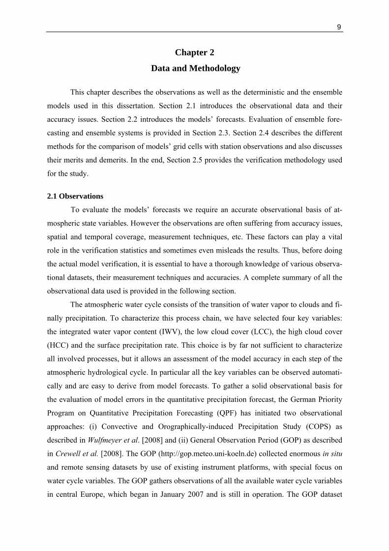
This chapter describes the observations as well as the deterministic and the ensemble
models used in this dissertation. Section 2.1 introduces the observational data and their
accuracy issues. Section 2.2 introduces the models’ forecasts. Evaluation of ensemble fore-
casting and ensemble systems is provided in Section 2.3. Section 2.4 describes the different
methods for the comparison of models’ grid cells with station observations and also discusses
their merits and demerits. In the end, Section 2.5 provides the verification methodology used
for the study.
2.1 Observations
To evaluate the models’ forecasts we require an accurate observational basis of at-
mospheric state variables. However the observations are often suffering from accuracy issues,
spatial and temporal coverage, measurement techniques, etc. These factors can play a vital
role in the verification statistics and sometimes even misleads the results. Thus, before doing
the actual model verification, it is essential to have a thorough knowledge of various observa-
tional datasets, their measurement techniques and accuracies. A complete summary of all the
observational data used is provided in the following section.
The atmospheric water cycle consists of the transition of water vapor to clouds and fi-
nally precipitation. To characterize this process chain, we have selected four key variables:
the integrated water vapor content (IWV), the low cloud cover (LCC), the high cloud cover
(HCC) and the surface precipitation rate. This choice is by far not sufficient to characterize
all involved processes, but it allows an assessment of the model accuracy in each step of the
atmospheric hydrological cycle. In particular all the key variables can be observed automati-
cally and are easy to derive from model forecasts. To gather a solid observational basis for
the evaluation of model errors in the quantitative precipitation forecast, the German Priority
Program on Quantitative Precipitation Forecasting (QPF) has initiated two observational
approaches: (i) Convective and Orographically-induced Precipitation Study (COPS) as
described in Wulfmeyer et al. [2008] and (ii) General Observation Period (GOP) as described
in Crewell et al. [2008]. The GOP (http://gop.meteo.uni-koeln.de) collected enormous in situ
and remote sensing datasets by use of existing instrument platforms, with special focus on
water cycle variables. The GOP gathers observations of all the available water cycle variables
in central Europe, which began in January 2007 and is still in operation. The GOP dataset

10 Data and Methodology
encompasses data collected by rain gauges, weather radars, micro rain radars, polarimetric
radars, disdrometers, ceilometers, GPS water vapor observations, lightning networks, satel-
lites, radiosondes, and special meteorological observation sites (e.g., CloudNET stations).
Figure 2.1: Central Europe topographical map indicating the D-PHASE domain (yellow
rectangle), the verification domain “Southern Germany” (thick black contour), the GPS
network (white circles), and the ceilometer network (red stars).
2.1.1 GPS Network to Observe IWV
The atmospheric integrated water vapour content (IWV) can be derived from ground-
based observations of the Global Positioning System (GPS). The studies by Tregoning et al.
[1998] and Doerflinger et al. [1998] showed that GPS-measured IWV has similar accuracy as
other instruments such as radiosondes and the water vapour radiometers. Continuous opera-
tions of GPS instruments in all weather conditions along with the fairly dense network make
them very useful for verification of model IWV. The IWV measurement by GPS is based on
the propagation delay of microwave signals (1.2 and 1.5 GHz, L-Band) transmitted by the
GPS satellite to the receiver. The delays can be estimated using high precision GPS satellite
orbits and receiver positions. This delay in the microwave signal occurs due to the different
atmospheric constituent called a total zenith delay (ZTD), which can be expressed as a zenith
hydrostatic delay (ZHD, about 90% of total zenith delay) and zenith wet delay (ZWD). The
hydrostatic delay is caused by the dry atmospheric components which only depend on the
total pressure and the temperature. Davis et al. [1985] shown that the ZHD is accurately
estimated from the surface pressure and air temperature. The remaining wet delay, ZWD, is
induced by the interaction of the GPS signal with the permanent dipole moment of water
vapor molecules. The ZWD is taken as difference between the observed total delay and the

11 Data and Methodology
hydrostatic delay [Dick et al., 2001], and is closely related to the integrated water vapor. Note
that IWV retrievals require very accurate delay observations and data analysis schemes
because a difference of 1 kg/m2 in IWV corresponds only to change in ZWD of ~6 mm.
These demands can only be achieved by networks of GPS receivers. Studies by Van Baelen et
al. [2005] and Niell et al. [2001] demonstrated that GPS derives IWV over land with an
accuracy of 1-2 kg/m². The German Research Centre for Geosciences (GFZ) provides near
real-time IWV observations from GPS during GOP with a temporal resolution of 15 minutes
and delay accuracy of 1-2 mm is equal to accuracy of ~0.3 kg/m² in IWV [Crewell et al.,
2008]. The German GPS network consisting of approximately 200 stations and our study
domain (Southern Germany) comprises 63 GPS stations (see Figure. 2.1).
2.1.2 Ceilometer Network to Observe LCC
A ceilometer is a simple lidar (Light Detection And Ranging)-based instrument which
measures the cloud-base height. Lidar transmits a laser pulse in the specific direction, and
receives the backscatter light from air molecules, aerosols and cloud droplets with a receiver
telescope. The delay in return signal indicates the altitude and intensity of the light represents
the concentration. Due to the low power operation and relatively long wavelength (λ~910nm,
λ~1030nm), ceilometers can operate continuously in any weather condition with low opera-
tion cost. The ceilometer system detects clouds by transmitting pulses of infrared light
vertically into the atmosphere. The receiver telescope detects backscattered light from water
droplets or aerosols. The strength of the backscattered signal depends on the amount of
scattering particles in a volume and their respective scattering efficiency. The time interval
between transmission and reception of the signal determines the height range of the scattering
volume. The cloud-base height is derived as an average height between the maximum
backscatter and the largest vertical gradient in backscatter signals. The maximum gradient of
backscatter signal is also used along with the maximum backscatter because the vertical
changes in aerosol/hydrometeor concentration dominate the received signals at long (λ~1 μm)
wavelength [Martucci et al., 2010]. The ceilometers are able to detect multiple cloud layers
simultaneously, providing cloud thickness where the layers do not totally attenuate the laser
beam. The cloud-base height derived from ceilometers might be biased towards lower values
due to the altitude limitation. Altitude limitation is mostly caused by long pulse length and
sensitivity of ceilometer detection, which then depends upon the ceilometer type. The accura-
cy of ceilometer cloud-base height is better than 30 m. The studies by Van Meijgaard and
Crewell [2005] inferred that, as backscatter gradients of ice clouds are weaker, ceilometers

12 Data and Methodology
often do not detect them. Hence ceilometers are well suited to study the low-level water
clouds. The German Meteorological Service (DWD) provides ceilometer observations of
more than 100 stations during GOP with a temporal resolution of 10 minute and cloud-base
accuracy of 30 m [Crewell et al., 2008]. Our study domain (Southern Germany) comprises 33
ceilometer stations (see Figure 2.1).
2.1.3 MSG based Retrieval of HCC
The Meteosat Second Generation (MSG) is a geostationary satellite developed by the
European Space Agency (ESA) and operated by the European Organization for the Exploita-
tion of Meteorological Satellites (EUMETSAT). The MSG covers the views of Europe,
Africa, and much of the Atlantic Ocean every 15 minutes and provides an excellent database
to study the diurnal variation of cloud systems. The Spinning Enhanced Visible and InfraRed
Imager (SEVIRI) on MSG has 12 spectral channels with 4 VIS/NIR channels (0.4 - 1.6 µm)
and 8 IR channels (3.9 - 13.4 µm). Our analysis is based on cloud products derived at the
Institute for Space Sciences at the Free University of Berlin, Germany (FUB). The cloud
product in FUB is derived from algorithms based on artificial neural networks which use
Assumed Clear Sky Brightness Temperature (ACSBTE) of the 10.8 μm channel as the main
input parameter [Reuter, 2005]. The ACSBTE algorithm uses assumptions of smoothness in
the diurnal cycles of surface temperature, their possibility to change with time, and that
clouds generally appear colder than the underlying surface in the 10.8 μm channel. Reuter
[2005] shows that ACSBTE values in the 10.8 μm channel can be derived at an accuracy of ±
3.3 K. The viewing and solar geometry information and measurements of the SEVIRI chan-
nels at 13.4, 12.0, 10.8, 8.7, 3.9, 1.6, 0.8, and 0.6 μm are used as additional input parameters
for the artificial neural network. Manual classification of cloudy and clear sky pixels were
used to train data for the neural network. The output of the network represents the cloud
probability at pixel level which can be interpreted as a mathematical probability that a
satellite pixel is cloudy.
The cloud-top pressure from the SEVIRI is derived using the CO2 slicing method.
Due to the constant mixing ratio of CO2 in the atmosphere the weighting function of 13.4
μm channel shows significant sensitivity in all pressure levels. The CO2 slicing method uses
the difference between the 13.4 μm CO2 absorption channel and 12 μm infrared channels to
derive the cloud-top pressure [Brusch, 2006]. Reuter et al. [2009] shows that the FUB
retrievals agree better in daytime with the synoptic stations compared to nighttime, because
the additional information from SEVIRI solar channels is not available in nighttime. Howev-
13 Data and Methodology
er, Reuter [2005] shows that nighttime retrievals improve considerably by using ACSBTE.
The hourly cloud product from FUB is utilized in this study because the model forecasts are
available at hourly basis. The FUB cloud product is derived on a normalized geostationary
projection with horizontal resolution of approximately 5 km [Reuter, 2005]. The accuracy of
CTP is approximately 52 hPa for high clouds [Crewell et al., 2008].
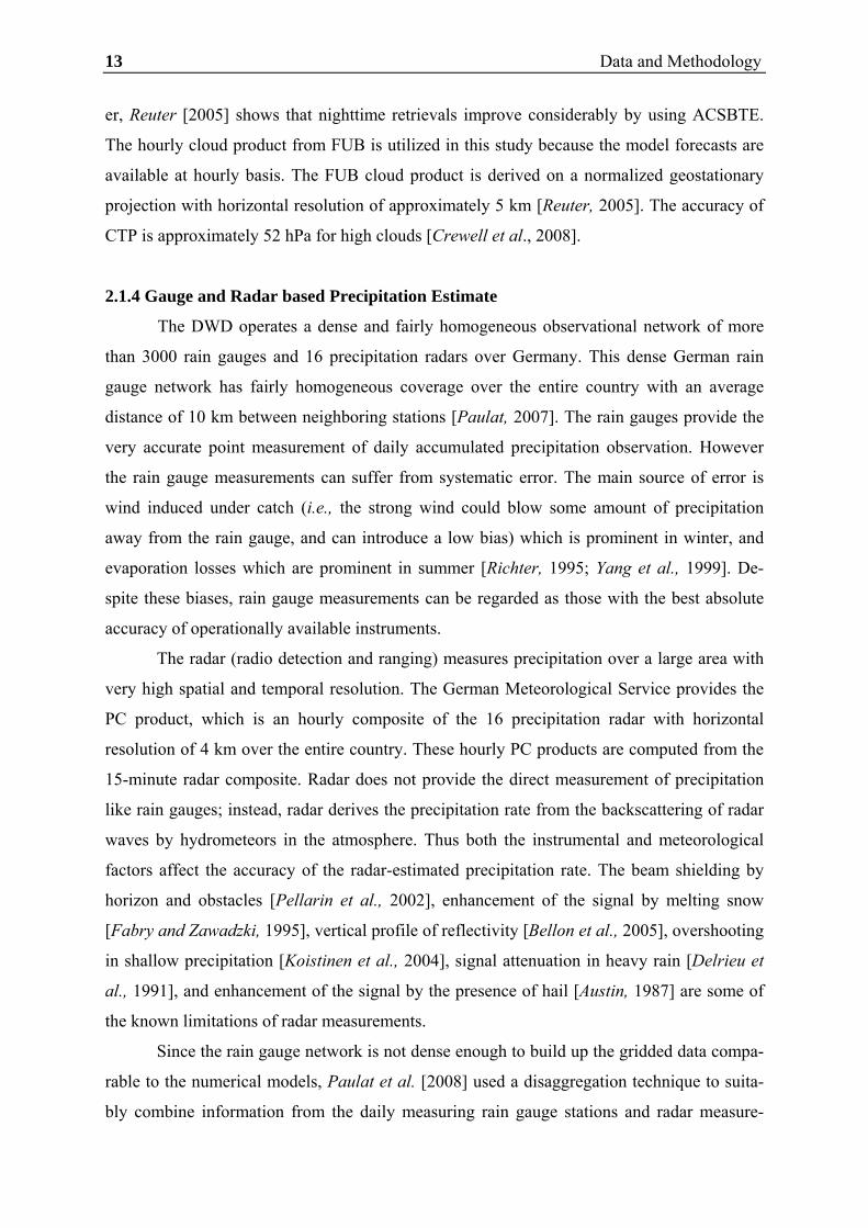
2.1.4 Gauge and Radar based Precipitation Estimate
The DWD operates a dense and fairly homogeneous observational network of more
than 3000 rain gauges and 16 precipitation radars over Germany. This dense German rain
gauge network has fairly homogeneous coverage over the entire country with an average
distance of 10 km between neighboring stations [Paulat, 2007]. The rain gauges provide the
very accurate point measurement of daily accumulated precipitation observation. However
the rain gauge measurements can suffer from systematic error. The main source of error is
wind induced under catch (i.e., the strong wind could blow some amount of precipitation
away from the rain gauge, and can introduce a low bias) which is prominent in winter, and
evaporation losses which are prominent in summer [Richter, 1995; Yang et al., 1999]. De-
spite these biases, rain gauge measurements can be regarded as those with the best absolute
accuracy of operationally available instruments.
The radar (radio detection and ranging) measures precipitation over a large area with
very high spatial and temporal resolution. The German Meteorological Service provides the
PC product, which is an hourly composite of the 16 precipitation radar with horizontal
resolution of 4 km over the entire country. These hourly PC products are computed from the
15-minute radar composite. Radar does not provide the direct measurement of precipitation
like rain gauges; instead, radar derives the precipitation rate from the backscattering of radar
waves by hydrometeors in the atmosphere. Thus both the instrumental and meteorological
factors affect the accuracy of the radar-estimated precipitation rate. The beam shielding by
horizon and obstacles [Pellarin et al., 2002], enhancement of the signal by melting snow
[Fabry and Zawadzki, 1995], vertical profile of reflectivity [Bellon et al., 2005], overshooting
in shallow precipitation [Koistinen et al., 2004], signal attenuation in heavy rain [Delrieu et
al., 1991], and enhancement of the signal by the presence of hail [Austin, 1987] are some of
the known limitations of radar measurements.
Since the rain gauge network is not dense enough to build up the gridded data compa-
rable to the numerical models, Paulat et al. [2008] used a disaggregation technique to suita-
bly combine information from the daily measuring rain gauge stations and radar measure-

14 Data and Methodology
ments. The disaggregation method is designed to exploit temporal information from radar
while maintaining maximum consistency with the daily measurements from the rain gauge
networks. Initially daily gauge sums are gridded on a cartesian grid by a statistical interpola-
tion scheme adopted from Frei and Schär [1998]. This interpolation technique is based on an
angular distance-weighting scheme. This scheme calculates the two components of weight
within the search radius, and the search radius is chosen in such a way that at least three
stations contribute to the averaging. At first, all stations are weighted by distance from the
grid point, with the empirically derived decorrelation length scale controlling the rate at
which the weight decreases with distance from the grid point. Second the distance-weight
component is determined by the directional (angular) isolation for each of the stations. Using
a second weighting particularly helps to improve the performance of the analysis along the
boundaries between high and low resolution networks as clusters of observations to one side
of the grid point are appropriately down-weighted.
To consider the effect of the poor rain gauge network in the mountainous terrain, Pau-
lat et al. [2008] used the detrended kriging approach of Widmann and Bretherton [2000]. The
high resolution precipitation climatology of the DWD over Germany for the years 1961-1990
[Müller-Westermeier, 1995] is used for kriging. The climatology provides the explicit height
gradients on 1 km horizontal resolution. Thus, in the detrended kriging approach, the daily
fractional rain gauge totals from the interpolation are multiplied by the gridded collocated
climatological anomalies. Frei et al. [2003] shows that the detrended kriging approach
increases area mean precipitation values in the Alpine region of Southern Germany by
typically 5-15% and does not have a major effect elsewhere.
Paulat et al. [2008] aggregated both the gridded daily rain gauge data and radar com-
posites on grids identical to the COSMO-7 model operated by MeteoSwiss with a horizontal
resolution of 7 km. This gridded product of daily precipitation is then temporally disaggre-
gated by fractioning the daily total rain gauge values according to contribution considered
from hourly radar estimate at every individual grid box. The basis of this technique is to
combine fairly dense and highly accurate rain gauges with the high spatial and temporal
resolution radar observations. This technique uses radar observations only to enhance tem-
poral resolution of rain gauge measurements and does not use the spatial information provid-
ed by radar observations, as this technique aims to retain the high accuracy of rain gauge
measurements, to keep the consistency with daily analyses from rain gauges alone and to
avoid effects from radar biases [Paulat et al., 2008].

15 Data and Methodology
2.2 Model Description
Knowledge of the model configuration, such as grid spacing, initial condition, along
with the physical parameterization is crucial for interpretation of verification results. The
section below introduces the basic models’ configurations, and provides a brief description of
the different physical parameterization schemes used, as well as the data assimilation meth-
ods.
The model output used for the verification in our study is gained by the MAP D-
PHASE experiment (Mesoscale Alpine Program - Demonstration of Probabilistic Hydrologi-
cal and Atmospheric Simulation of flood Events) in the Alpine region [Rotach et al., 2009].
The Mesoscale Alpine Programme (MAP) was first a research and development project of
the World Weather Research Programme (WWRP) which was initiated to understand the
atmospheric processes influencing weather in mountainous terrain [Bougeault et al., 2001;
Volkert, 2005]. D-PHASE was a forecast demonstration experiment of MAP. The main
objective was to demonstrate the benefits in forecasting heavy precipitation and related flood
events, as gained from the improved understanding, refined atmospheric and hydrological
modeling, and advanced technological abilities acquired through research work during the
MAP. D-PHASE was operated as a real time end-to-end heavy precipitation and flood
warning system from June to November 2007 to demonstrate the state-of-the-art forecasting
of precipitation related to high impact weather. Throughout the forecasting chain, warnings
were issued and re-evaluated as the potential flooding event approached, allowing forecasters
and end users to be alerted and make decisions in due time [Rotach et al., 2009]. More than
25 mesoscale models and 6 ensemble systems provided both real-time precipitation forecasts
and stored a comprehensive set of forecast fields in a central data archive for latter evalua-
tion. The target region of D-PHASE covered the entire Alpine region and adjacent areas (see
yellow box in Figure 2.1).
All model providers contributed to D-PHASE on a voluntary basis without any fund-
ing. Consequently the quality and completeness of the model data in the D-PHASE data
archive varies considerably; for example, not all model forecasts covered the whole D-
PHASE domain or reported all required variables. To ensure a fair model comparison in our
evaluation, we considered only those models which fulfill the following three criteria: (i) all
four key variables (IWV, LCC, HCC and precipitation rate) are reported. (ii) the model
domains cover at least 95% of the Southern Germany verification domain. (iii) data are
available for at least 95% of the time from June to August 2007. Table 2.1 lists the 9 models
which satisfy our selection criteria.

16 Data and Methodology
Table 2.1 lists the basic configuration of selected models such as horizontal resolu-
tion, forecast range, initiation frequency, driving model and the operational institute. As
shown in Table 2.1 this ensemble of 9 models provides clusters of models sharing certain
features: e.g. models based on the same model physics, models sharing the same boundary
conditions, convection-resolving and convection-parameterized models and models with
different data assimilation methods. The models can be sorted into three groups with respect
to the model code COSMO, French, and MM5. The COSMO models are developed by the
Consortium for Small-Scale Modelling (COSMO) and are designed for the operational NWP
and climate simulations. COSMO-DE and COSMO-EU are operated by DWD, whereas
COSMO-2 and COSMO-7 by MeteoSwiss and COSMO-IT and COSMO-ME by CNMCA
(National Meteorological Center) Italy. The French group of models AROME (Application of
Research to Operational at Mesoscale) and ALADFR are operated by Mètèo-France, while
MM5 model is operated by FZK IMK-IFU (Institute for Meteorology and Climate Research,
Atmospheric Environmental Research Division, Karlsruhe Institute of Technology) in
Germany.
Table 2.1: Summary of evaluated models (high resolution models are highlighted).
Model Grid
Spacing [km]
Forecast Range
[h]
Runs/day
Nested in Driving Global
Model Provided by
COSMO-DE 2.8 21 8 COSMO-EU GME (DWD) DWD COSMO-EU 7 78 4 GME GME (DWD) DWD COSMO-2 2.2 24 6 COSMO-7 IFS (ECMWF) Meteo-Swiss COSMO-7 7 72 2 IFS IFS (ECMWF) Meteo-Swiss COSMO-IT 2.8 30 1 COSMO-ME IFS (ECMWF) CNMCA COSMO-ME 7 72 1 IFS IFS (ECMWF) CNMCA AROME 2.5 30 1 ALADFR ARPEGE Meteo-France ALADFR 9.5 30 1 ARPEGE ARPEGE Meteo-France MM5 15 72 2 MM5_60 GFS (NOAA) FZK IMK-IFU
Out of 9 models, 4 models (COSMO-DE, COSMO-2, COSMO-IT, and AROME) are
high resolution models with horizontal grid spacing less than 3 km (see Table 2.1). These
high resolution models partially resolve convection, thus only shallow convection needs to be
parameterized and deep convection is explicitly calculated. The remaining 5 models (COS-
MO-EU, COSMO-7, COSMO-ME, ALADFR, and MM5) are coarse resolution models
which parameterize both shallow and deep convection (see Table 2.2). Hereafter, the high
resolution models are termed as HIGHRES models and coarse resolution models are termed
as LOWRES models. COSMO-DE and COSMO-2 have a very high frequency of reinitializa-
17 Data and Methodology
tion, i.e., 6-8 runs/day, however the forecast range is only 18 h for COSMO-DE and 24 h for
COSMO-2. In contrast the corresponding LOWRES models COSMO-EU and COSMO-7
have reinitialization frequencies of 4 and 2 runs/day respectively, and forecast ranges of 78
and 72 h respectively. COSMO-IT and COSMO-ME runs once a day with forecast ranges of
30 and 72 h respectively. The two French models were run once a day with a forecast range
of 30 h, where MM5 runs twice a day with a forecast range of 72 h. The COSMO-EU model
is driven by GME global models, COSMO-7 and COSMO-ME are forced by the ECMWF
(European Centre for Medium-Range Weather Forecasts) models. The boundary conditions
for ALADFR are provided by ARPEGE global model and for MM5 by NOAA GFS (Global
Forecast System) model. Note that all HIGHRES models are nested in their corresponding
LOWRES models.
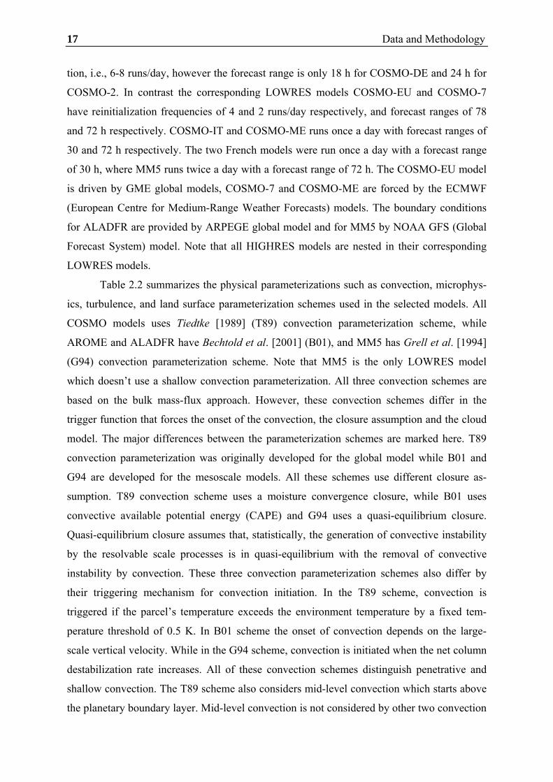
Table 2.2 summarizes the physical parameterizations such as convection, microphys-
ics, turbulence, and land surface parameterization schemes used in the selected models. All
COSMO models uses Tiedtke [1989] (T89) convection parameterization scheme, while
AROME and ALADFR have Bechtold et al. [2001] (B01), and MM5 has Grell et al. [1994]
(G94) convection parameterization scheme. Note that MM5 is the only LOWRES model
which doesn’t use a shallow convection parameterization. All three convection schemes are
based on the bulk mass-flux approach. However, these convection schemes differ in the
trigger function that forces the onset of the convection, the closure assumption and the cloud
model. The major differences between the parameterization schemes are marked here. T89
convection parameterization was originally developed for the global model while B01 and
G94 are developed for the mesoscale models. All these schemes use different closure as-
sumption. T89 convection scheme uses a moisture convergence closure, while B01 uses
convective available potential energy (CAPE) and G94 uses a quasi-equilibrium closure.
Quasi-equilibrium closure assumes that, statistically, the generation of convective instability
by the resolvable scale processes is in quasi-equilibrium with the removal of convective
instability by convection. These three convection parameterization schemes also differ by
their triggering mechanism for convection initiation. In the T89 scheme, convection is
triggered if the parcel’s temperature exceeds the environment temperature by a fixed tem-
perature threshold of 0.5 K. In B01 scheme the onset of convection depends on the large-
scale vertical velocity. While in the G94 scheme, convection is initiated when the net column
destabilization rate increases. All of these convection schemes distinguish penetrative and
shallow convection. The T89 scheme also considers mid-level convection which starts above
the planetary boundary layer. Mid-level convection is not considered by other two convection

18 Data and Methodology
schemes. The T89 and B01 schemes consider the entrainment and detrainment that occurs at
the lateral boundaries of cloud, while in the G94 scheme the mixing between cloud and
environment occurs only at the cloud base and cloud top.
Table 2.2: Summary of different convective, microphysics, turbulence, and land surface
schemes, as well as assimilation methods considered in evaluated models (high resolu-
tion models are highlighted).
Model Convection Microphysics Turbulence Land Surface
Assimilation method
COSMO-DE T89 shallow D07M (r, s, g, cd, ic)*
D07T H06 Nudging
COSMO-EU T89 deep + shallow
D07M (r, s, cd, ic)*
D07T H06 ”
COSMO-2 T89 Shallow
D07M (r, s, g, cd, ic) *
D07T H06 ”
COSMO-7 T89 deep + shallow
D07M (r, s, cd, ic) *
D07T H06 ”
COSMO-IT T89 Shallow
D07M (r, s, g, cd, ic) *
D07T H06 ”
COSMO-ME T89 deep + shallow
D07M (r, s, cd, ic) *
D07T H06 3D-Var
AROME B01 Shallow
PJ98 (r, s, g, cd, ic) *
C00 NP89 ”
ALADFR B01 deep + shallow
PJ98 (r, s, cd, ic) *
C00 NP89 ”
MM5 G94 Deep
R98 (r, s, g, cd, ic) *
HP96 CD01
none
*Representing the applied hydrometeor classes: r for rain, s for snow, g for graupel, cd for cloud
droplets, ic for ice crystals. B01=Bechtold et al. [2001]; C00=Cuxart et al. [2000]; CD01=Chen and
Dudhia [2001]; D07M=Doms et al. [2007]; D07T=Doms et al. [2007]; G94=Grell et al. [1994];
H06=Heise at al. [2006]; HP96=Hong and Pan [1996]; NP89=Noilhan and Planton [1989];
PJ98=Pinty and Jabouille [1998]; R98=Reisner et al. [1998]; T89=Tiedke [1989]
All COMSO models use Doms et al. [2007] (D07M) microphysics scheme, while
AROME and ALADFR models has Pinty and Jabouille [1998] (PJ98) microphysical scheme,
and MM5 model use Reisner et al. [1998] (R98) microphysical scheme. All three of these
microphysics schemes are mixed-phase bulk schemes similar to Lin et al. [1983]. All
schemes predict five hydrometeor species, two non-precipitating (cloud water and cloud ice)
and three precipitating (rain, snow, and graupel) species. For all schemes hydrometeor
species are described by a prognostic mixing ratio which is determined through various

19 Data and Methodology
microphysical processes (e.g., condensation, evaporation, sublimation, fall-out, break-up,
collision). However, D07M and PJ98 scheme are one-moment schemes, they predicts only
the mixing ratio of all five hydrometeors species. R98 is a two-moment scheme, which
explicitly predicts the number concentration of cloud ice, snow, and graupel, along with
mixing ratio of five hydrometer species. In the D07M scheme, size distribution properties of
hydrometeors, such as the intercept, the slope, and the number concentrations are depend
upon precipitation amount for raindrops, while fixed intercept parameter is set for graupel.
For snow size distribution a temperature and mixing ratio dependent intercept parameter is
assumed in the D07M scheme. In the PJ98 scheme, the size distribution properties of hydro-
meteors depend upon the precipitation amount of individual hydrometeors. In the R98
scheme, the properties of size distribution are set constant except for snow; the intercept
parameter of snow is allowed to vary with the snow mixing ratio. All HIGHRES models
consider all five hydrometeors species, while all LOWRES models consider only four
hydrometeors species, except MM5 model. MM5 is the only LOWRES model considering
the graupel hydrometeor species.
In COSMO models turbulence is parameterized by Doms et al. [2007] (D07T) turbu-
lence scheme, while AROME and ALADFR use Cuxart et al. [2000] (C00) turbulence
scheme and MM5 has Hong and Pan [1996] (HP96) turbulence scheme. D07T and C00 are
local turbulence schemes, while HP96 is a non-local turbulence scheme. In D07T and C00,
representation of the turbulence in the planetary boundary layer is based on a prognostic
Turbulence Kinetic Energy (TKE) equation combined with a diagnostic mixing length. In
both of these schemes turbulence fluxes are calculated implicitly in time by the exchange
coefficients for momentum, potential temperature, and humidity using tri-diagonal matrix.
However, D07T and C00 schemes differ by the order of closure used, which refers to the
highest turbulent moment predicted. D07T scheme have 2.5 order closure, while C00 have
1.5 order closure. HP96 turbulence scheme is a first-order, non-local closure scheme. It
predicts tendencies of mixing ratio, potential temperature, horizontal wind, cloud water, and
cloud ice in four different regimes depending on the bulk Richardson number.
In COSMO models the surface layer is parameterized by Heise et al. [2006] (H06)
scheme, while AROME and ALADFR use Noilhan and Planton [1989] (NP89) surface
scheme and MM5 has Chen and Dudhia [2001] (CD01) surface layer scheme. H06 uses a 10-
layer soil model with prognostic soil moisture for top 7 layers. NP89 has three soil layers
with prognostic soil moisture, while CD01 have four soil layers with prognostic soil mois-
ture.

20 Data and Methodology
All COSMO models use a nudging data assimilation method, except COSMO-ME
model which uses 3D-Var data assimilation method. Both French models AROME and
ALADFR use 3D-Var data assimilation method. MM5 is the only model used in this study
which didn’t use any data assimilation. For further details of the models, the reader is asked
to refer to Arpagaus et al. [2009].
2.3 Ensemble Forecasting
Ensemble forecasting is a relatively new forecasting method. Detailed descriptions of en-
semble forecasting and different methods available for generating ensemble forecasts are
provided in this section. Finally, the ensemble systems we utilized in our evaluation are
described.
2.3.1 Introduction to Ensemble Forecasting
Numerical weather prediction has three basic components: observation of the atmos-
pheric state, assimilation of observed data into initial conditions, and model integration. The
uncertainties are introduced at each of these steps during a forecast process: for example,
instrumental errors in the observations, errors introduced during data assimilation due to
mathematical assumptions, and imperfect parameterizations in models. Due to its highly
nonlinear nature, numerical weather prediction is chaotic in nature. Smaller differences in
initial states could lead to very different realizations in future states in such a chaotic system
[Lorenz, 1963]. To account for this chaotic nature, the forecast uncertainty is also necessary
to predict. Ensemble forecasting is a dynamical and flow-dependent approach to quantifying
such forecast uncertainty.
Ensemble forecasting aims to incorporate all possible uncertainty sources in a model-
ing system accurately and completely in terms of perturbations, and integrates the model in
time to produce an ensemble of forecasts. The ensemble forecast consists of the multiple
model runs initiated with the different perturbations. Generation of ensemble prediction
systems (EPS) can be grouped into three categories: 1-D, 2-D and 3-D EPS [Du, 2007]. The
ensemble systems which consider uncertainty only due to the initial conditions are called 1-D
EPS [Li et al., 2008]. The 2-D EPS consider the uncertainty due to the models physics and
dynamics along with the initial conditions [Du and Tracton, 2001]. Multi-model, multi-
physics, multi-dynamics, multi-ensemble systems are examples of the 2-D EPS. In 3-D EPS,
past memory or history is also considered in addition to uncertainty due to the initial condi-
tions, model physics and dynamics. The direct time-lagged approach is usually used to

21 Data and Methodology
consider the past memory [Lu et al., 2007]. There are multiple approaches to produce the
perturbations for generation of the ensemble system. The random perturbation approach uses
the Monte Carlo method to generate the perturbations, where a normal distribution is used to
represent typical uncertainty in the analysis [Mullen and Baumhefner, 1994]. The Time-
Lagged approach considers model runs which are initiated at different times [Mittermaier,
2007]. This approach is considered to lead to a larger ensemble spread compared to random
perturbations, as it reflects the error of the day [Du, 2007]. The Breeding approach uses
multiple concurrent forecasts rather than a time-lagged forecast and a current analysis to
calculate raw perturbations [Toth and Kalnay, 1997]. The Singular Vector approach uses the
linear version of a nonlinear model as well as an adjoint of the time lag method to generate
the perturbations [Li et al., 2008]. The coupled data-assimilation / perturbation-generation
approach uses multiple analyses available to initiate an ensemble of forecasts [Grimit and
Mass, 2002].
2.3.2 Description of Ensemble Systems
For the verification we have selected 3 limited area ensemble systems, COSMO-
LEPS (CLEPS), COSMO-SREPS (CSREPS), and LAMEPSAT, from the MAP D-PHASE
experiment with the same criteria used for deterministic models selection (Section 2.2).
However, LAMEPSAT does not report the IWV (see Table 2.3). We have also generated a
poor man ensemble system (PEPS) from 9 different deterministic (see Table 2.3) MAP D-
PHASE models. As deterministic models are used to generate ensemble forecast which
operated by different operational or research centres, no additional cost is required to gener-
ate ensemble forecasts, and hence is called as poor-man ensemble system.
CLEPS is a limited-area ensemble prediction system based on a non-hydrostatic
COSMO model implemented by ARPA-SIM (Regional Hydro-Meteorological Service of
Emilia-Romagna, Italy) in the framework of the COSMO consortium [Marsigli et al. 2005].
CLEPS uses a downscaling of the ECMWF 51-member global ensemble system. This high
resolution EPS is developed to improve early and medium-range (3-5 days) predictability of
extreme and localized mesoscale weather events. The size of the ensemble is limited to 16
members to decrease the computational expenses of running high resolution EPS with large
ensemble size. The 51 members of ECMWF EPS are divided into 16 clusters, and one
member of each cluster provides the initial and boundary conditions for the COSMO models
once a day. The small-scale error due to model uncertainty is sampled by the use of different

22 Data and Methodology
convective parameterization schemes (Tiedtke or Kain-Fritsch). The EPS runs once a day
with horizontal resolution of 10 km and forecast range of 132 hours.
CSREPS is a short-range (up to 3 days) high resolution ensemble prediction system
based on COSMO model provided by ARPA-SIM [Marsigli, 2009]. The system consists of
16 integrations of the non-hydrostatic limited-area model COSMO. CLEPS mainly considers
large-scale uncertainty through perturbations of initial and boundary conditions from
ECMWF EPS; thus, it is useful especially in the early medium-range forecasts (day 3-5).
Unlike CLEPS, CSREPS considers the large-scale uncertainty through different driving
models, as well as small-scale uncertainty through limited-area models to account for all
possible uncertainty in the high resolution short-range forecast. Initial and boundary condi-
tion perturbations are provided by some members of the Multi-Analysis Multi-Boundary
SREPS system of INM (Spanish Met Service): the 10-km COSMO runs of COSMO-SREPS
are driven by four low resolution (25 km) COSMO runs provided by INM, nested on four
different global models (Integrated Forecast System (IFS), Global Unified Model (UM),
Global Forecast System (GFS), and Global Model (GME)) which use independent analyses.
Each of the four 25-km COSMO runs provides initial and boundary conditions to four 10-km
COSMO runs, which are differentiated by applying different model perturbations. Four
parameters of the parameterization are randomly changed within their range of variability
such as the Tiedtke and Kain-Fritsch convection schemes and the maximal turbulent length
scale (tur_len) and length scale of thermal surface patterns (pat_len). The CSREPS ensemble
system runs once in a day with a horizontal resolution of 10 km and forecast range of 72 h.
LAMEPSAT is the ALADIN-Austria Ensemble system operated by ZAMG (Austri-
an Meteorological Service) based on the ALADIN model [Wang et al., 2006]. Only perturba-
tions in initial and boundary conditions are applied which are representative of large-scale
errors (see Table 2.3). The initial-condition perturbations are generated by down-scaling the
ECMWF singular vector perturbation, while lateral boundary perturbations are generated by
coupling with the ECMWF ensemble system. This 16 member ensemble system runs twice a
day with a horizontal resolution of 18 km and forecast range of 48 h.
PEPS is a poor man ensemble system generated from the 9 MAP D-PHASE deter-
ministic models (see Table 2.3). The ensemble forecast is generated by up-scaling all 9
deterministic models on to a common horizontal grid of 21 km. The forecast uncertainty due
to the large-scale error and also due to the small-scale error are accounted, as models with the
four different initial conditions and three different model physics are included. The forecast

23 Data and Methodology
range of PEPS is only 21 h as we want to consider all 9 models’ forecasts and COSMO-DE is
limited to this range.

24 Data and Methodology
2.4 Comparison of Models grid-cell with Station Observations
Comparing point observations with the model grid cell is challenging, as they have an
inherent mismatch between the spatial scales. Most ground-based instruments provide point
measurements. Models, on the other hand, predict the area-mean value of the variable within
the grid cell. There are a number of studies which address this issue; here we discuss some of
these approaches, their strengths and weaknesses.
The simplest approach is to directly compare the observation with the model grid cell.
Direct comparison can lead to serious errors as observations are representative of the point
whereas the model data represents the grid-mean value. However, this approach doesn’t add
any artifacts to the observations. Another approach is to average temporally the observations,
assuming that advection over time provides the same statistics as would be gathered from
observing instantaneous spatial variability [e.g., Barnett et al., 1998]. In this approach the
averaging time is calculated based on the wind speed at specific times which will vary with
model resolution. However, most of these studies average over fixed time intervals, even
though the resulting statistics can depend significantly on which interval is chosen [Hogan
and Illingworth, 2000]. Jakob [2004] argued that matching of grid cell size and time-
averaging intervals is misleading, as it depends on the meteorological conditions (e.g., wind
speed, presence of convection and frontal system).
Jakob [2004] proposed a probabilistic approach for comparison of station cloud ob-
servations with the model grid cell values. This approach assumes that clouds are randomly
distributed throughout the domain. With the above assumption, a cloud cover forecast can be
considered as the probability at a specific station and time. This approach is conceptually
appealing because they bridge the disparities of scales without reducing the information
content of the observations or relying on time averaging. However, it requires different
verification metrics which are appropriate for probabilistic rather than deterministic forecasts.
This increases the complexity of the interpretation of the results.
Ghelli and Lalaurette [2000] proposed the up-scaling approach in which the observa-
tions are up-scaled to the models grid cell. However, the number of observational stations in
each grid cell varies considerably, and the intercomparison of models with different resolu-
tions is difficult. A similar approach was proposed by Marsigli et al. [2008], called the
distribution method (DIST), which is based on the verification distribution parameter within
boxes of selected size. In this technique the verification domain is subdivided into a number
of boxes, each of them containing a certain number of observed and forecasted values. The
verification is performed using a categorical approach, by comparing for each box each

25 Data and Methodology
parameter of the forecast distribution such as mean, median, percentiles or maximum of the
observed distribution. This approach is very simple and quite intuitive in terms of the inter-
pretation of the verification results. Also local weaknesses of the model are not identified
because of averaging over large areas. We adopted the direct comparison approach as it does
not add any artifacts in the verification result. The next section shows how a simple direct
comparison approach can be used with little modification for different variables.
2.5 Verifications Methodology
Although the GOP comprises the whole of central Europe, certain observations such
as cloud-base height from ceilometers and gridded rain gauge data sets are limited to Germa-
ny. In this study, all verifications are restricted to the overlapping region where both observa-
tions and models forecast for all key variables are available (Southern Germany- Figure 2.1).
The largest amount of data is available in summer 2007 for both models and observations, as
the intense observing period COPS [Wulfmeyer et al., 2008] of the priority program took
place. Thus our study is focused exclusively for the summer period June to August 2007. The
different comparison strategies are presented for station observation to model grid cell as
explained in the previous section. We have adopted the nearest model grid-cell strategies for
IWV and LCC, and up-scaling for gridded HCC and gridded precipitation. In the following
section we will briefly explain the verification methodology adopted for all these key varia-
bles.
IWV: To compare the model grid cell with the station observation we use the grid cell
search strategy by Kaufmann [2008] which considers not just single grid cells horizontally
closest to the station but also the neighboring cells in a square of 5x5 grid cells. Among this
sample we selected the grid cell with the smallest effective distance, which is defined by the
sum of the horizontal distance plus the vertical distance enhanced by a factor of 500. Even
after this optimized search strategy, there will be a height difference between GPS station and
the model topography at the assigned grid cell. The horizontal displacement between obser-
vation sites and model grid points has a minor effect on the evaluation since GPS IWV is
determined from a number of delays to different satellites in different directions within 15
minutes. However, previous study by Guerova et al. [2003] reported that height differences
of a few meters between model grid cell and GPS station can introduce systematic errors.
Thus, to compare the model grid cell with the station observation, a correction factor due to
the height difference needs to be applied. The height difference can be minimized by a
careful selection of the model grid cell which is assigned to a certain measuring station.

26 Data and Methodology
When this remaining height difference is larger than 100 m, we have neglected those stations
from the evaluation. Otherwise we assumed that the modeled water vapor content at the
lowest model level is a good proxy for that in the lower height range. Then the modeled IWV
value can be corrected by adding
∆IWV = h
dzq mvm0
2,2 (2.1)
where the height difference ∆h is between the model grid cell and corresponding station, qv,2m
is the specific humidity and 2m is the air density at 2m level [Guerova et al., 2003]. Since
model output in the D-PHASE data archive is stored only in hourly intervals, we considered
only every fourth GPS observation in time, i.e. the observational interval centered on a clock
hour.
LCC: Cloud-base heights have not been reported by the D-PHASE models, and in
addition cloud base height is a poorly define variable (in case of partial cloudiness). There-
fore we have converted the ceilometer base height into binary information, which represents
whether there is a low cloud present or not. Only low level cloud cover is derived from the
ceilometer cloud base height as mid and high level clouds are often not detected by ceilome-
ter (Section 2.1.2). Low clouds are defined in the D-PHASE data archive as clouds below
1200 m. This binary low-cloud cover with values of either zero or one is used as an observa-
tional reference. In order to ensure a fair comparison, the model-predicted low-cloud cover is
also transformed into binary form using the unbiased threshold of 0.5. All model grid cells
with a low-cloud cover larger than 50% LCC are considered as overcast and the remaining
grid cells as clear sky. The choice of the threshold has no large impact, as the frequency
histogram (Figure 2.2) of almost all model predicted low cloud covers is strongly U-shaped.
For comparison of observed cloud cover from ceilometer to model, the nearest model grid
cell to the ceilometer station has been selected. Since model output in the D-PHASE data
archive is stored only in hourly intervals, we only considered every sixth ceilometer observa-
tion in time, i.e. the observational interval centered on a clock hour. The use of a threshold
instead of comparing all possible cloud amounts significantly decreases the uncertainties due
to the comparison of model grid cell with the station observation.
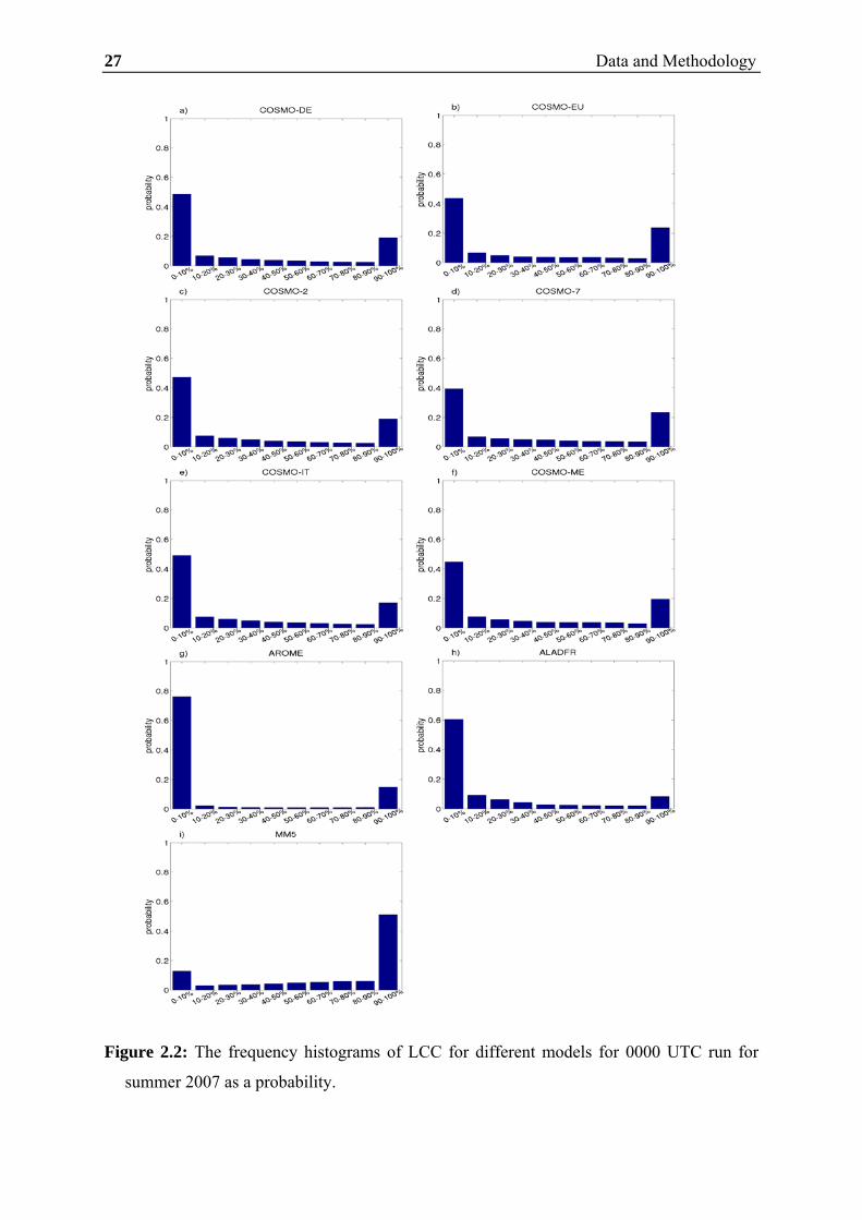
27 Data and Methodology
Figure 2.2: The frequency histograms of LCC for different models for 0000 UTC run for
summer 2007 as a probability.

28 Data and Methodology
Figure 2.3: Same as Figure 2.2, but for HCC.
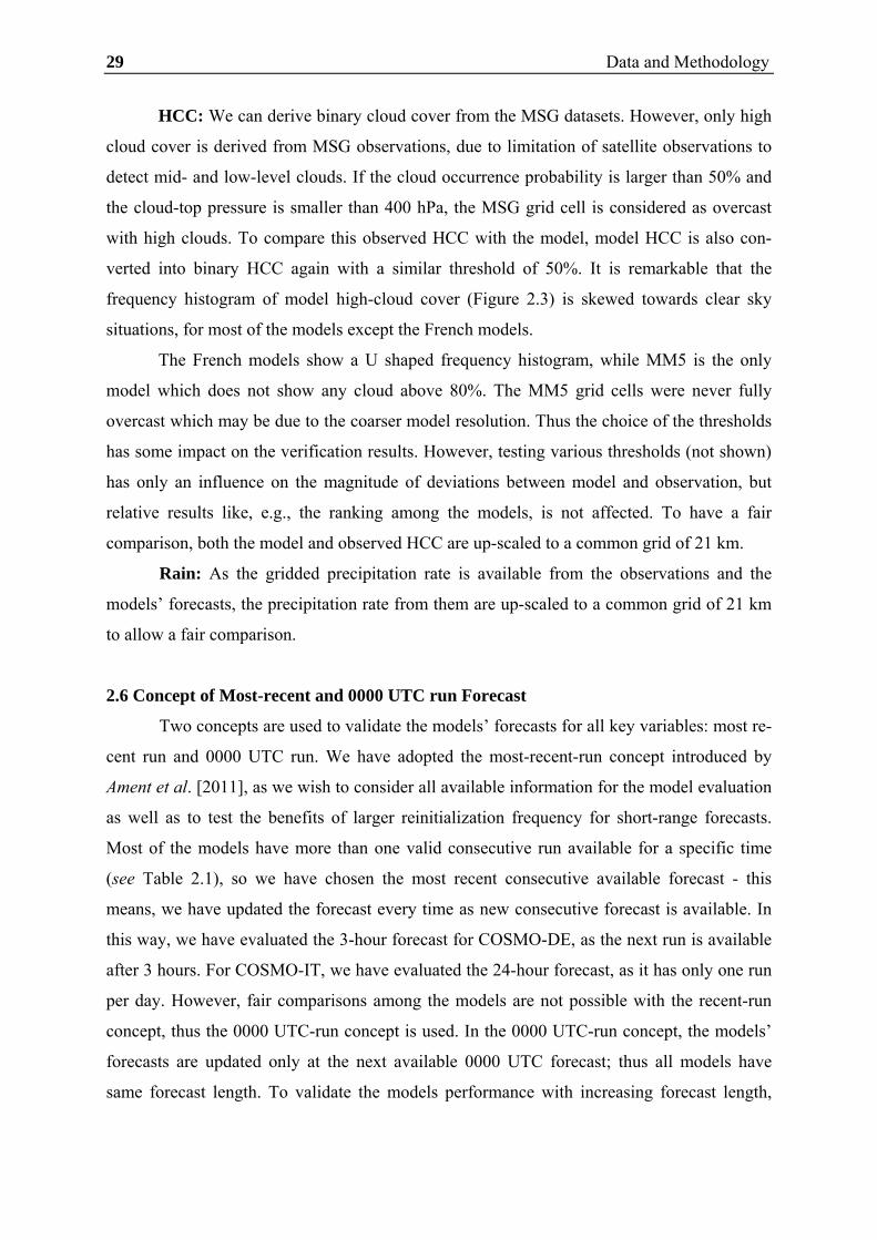
29 Data and Methodology
HCC: We can derive binary cloud cover from the MSG datasets. However, only high
cloud cover is derived from MSG observations, due to limitation of satellite observations to
detect mid- and low-level clouds. If the cloud occurrence probability is larger than 50% and
the cloud-top pressure is smaller than 400 hPa, the MSG grid cell is considered as overcast
with high clouds. To compare this observed HCC with the model, model HCC is also con-
verted into binary HCC again with a similar threshold of 50%. It is remarkable that the
frequency histogram of model high-cloud cover (Figure 2.3) is skewed towards clear sky
situations, for most of the models except the French models.
The French models show a U shaped frequency histogram, while MM5 is the only
model which does not show any cloud above 80%. The MM5 grid cells were never fully
overcast which may be due to the coarser model resolution. Thus the choice of the thresholds
has some impact on the verification results. However, testing various thresholds (not shown)
has only an influence on the magnitude of deviations between model and observation, but
relative results like, e.g., the ranking among the models, is not affected. To have a fair
comparison, both the model and observed HCC are up-scaled to a common grid of 21 km.
Rain: As the gridded precipitation rate is available from the observations and the
models’ forecasts, the precipitation rate from them are up-scaled to a common grid of 21 km
to allow a fair comparison.
2.6 Concept of Most-recent and 0000 UTC run Forecast
Two concepts are used to validate the models’ forecasts for all key variables: most re-
cent run and 0000 UTC run. We have adopted the most-recent-run concept introduced by
Ament et al. [2011], as we wish to consider all available information for the model evaluation
as well as to test the benefits of larger reinitialization frequency for short-range forecasts.
Most of the models have more than one valid consecutive run available for a specific time
(see Table 2.1), so we have chosen the most recent consecutive available forecast - this
means, we have updated the forecast every time as new consecutive forecast is available. In
this way, we have evaluated the 3-hour forecast for COSMO-DE, as the next run is available
after 3 hours. For COSMO-IT, we have evaluated the 24-hour forecast, as it has only one run
per day. However, fair comparisons among the models are not possible with the recent-run
concept, thus the 0000 UTC-run concept is used. In the 0000 UTC-run concept, the models’
forecasts are updated only at the next available 0000 UTC forecast; thus all models have
same forecast length. To validate the models performance with increasing forecast length,

30 Data and Methodology
first a specific number of forecast hours are excluded from the time series, which is called the
cutoff period.

31
Chapter 3
Evaluation of Integrated Water Vapor, Cloud Cover and Precipitation Pre-
dicted by Mesoscale Models
This chapter is dedicated to evaluate the performance of MAP D-PHASE mesoscale
models with respect to the prediction of integrated water vapor, cloud cover and precipitation. In
detail, the following questions will be addressed: How accurate can these key variables be
forecasted by today’s mesoscale models? Are there clusters of models revealing the same kinds
of error? In particular, is the forecasting performance of convection-permitting, high resolution
models superior? What is the most important factor, e.g. boundary conditions, model formulation
or resolution, affecting the forecast performance? To answer these questions, the models’ fore-
casts of all key variables (IWV, LCC, HCC, and precipitation) are statistically evaluated for
amount, timing (temporal distribution), and regional distribution aspects. Section 3.1 explores
the spatially and temporally averaged model biases and forecast skill. Section 3.2 illustrates the
models’ ability in representation of temporal distribution of all key variables by means of domain
average diurnal cycle. The models’ ability to represent the regional distribution is evaluated in
Section 3.3 and the impact of the forecast range on the model’s skill is assessed in Section 3.4.
3.1 Spatial and Temporal Averaged Verification
The overall model performance is assessed by verifying domain- and time-averaged key
variables for systematic error and error at a specific time and station or grid cell (random error).
This analysis will quantify the models’ ability in correctly predicting the average amount of key
variables. The verification scores depend respectively on the type of variables, for continuous
key variables such as IWV and precipitation rate the systematic errors is assessed by bias (BIAS)
while random error by standard deviation (STD). The systematic and random error in categorical
quantities such as LCC and HCC are assessed by frequency bias (FBIAS) and equitable threat
score (ETS: Appendix A) respectively. The verification of all key variables is performed only for
0000 UTC model runs to have a fair model comparison (see Section 2.6). The significance of the
result is assessed by bootstrap resampling method using 95% and 5% quantile of 1000 bootstrap
sample (see Appendix B).

32 Evaluation of Individual Key Variables
Figure 3.1 depicts the errors of all models concerning the four key variables where sys-
tematic errors are represented by green bars. The yellow bars indicate the forecast accuracy on an
hourly basis at a certain station (for IWV and LCC) or grid cell (for HCC and precipitation). The
BIAS in IWV is less than 1.5 kg/m2 for most of the models. All the models, except French
models AROME and ALADFR, have a tendency to be too dry, and MM5 is the wettest model.
Large IWV biases in MM5 and French models are likely due to deficits in their driving models
ARPEGE and GFS respectively. Bouteloup et al. [2009] reported significant overestimation of
summer precipitation by ARPEGE model over Europe.
Figure 3.1: Verification scores averaged over the whole Southern Germany domain and the
whole time period summer 2007. (a) BIAS (green) and standard deviation (yellow) in IWV
(kg/m2), (b) frequency bias (green) and equitable threat score (yellow) in LCC of hourly sta-
tion time series, (c) same as (b) but for HCC and (d) bias (green) and standard deviation
(yellow) in precipitation (mm/h) of hourly gridded time series. (The HIGHRES models are
highlighted by bold letters; Error bars represent the 95% and the 5% quantiles of the distri-
bution determined by a bootstrapping).

33 Evaluation of Individual Key Variables
The errors at a particular time and station are significantly larger than systematic error,
which is reflected by STD on the order of 3 kg/m2. There is no great difference between
HIGHRES convection-permitting models and LOWRES models. However, these HIGHRES
models tend to be slightly wetter than their LOWRES counterparts and the STD is slightly
smaller. All models show small interquantile distances for systematic and random error, which
implies small uncertainty in results.
The systematic error in low cloud cover (LCC) is described by FBIAS which is the ratio
of forecasted and observed frequency. An unbiased forecast has FBIAS of 1, underestimated
forecasts results in FBIAS values between 0 and 1, and overestimations are reflected by values
between 1 and ∞. To display corresponding under and overestimation with the same size of a
bar, we express the FBIAS in decibels (dB) which is the logarithm of FBIAS multiplied by 10.
The FBIAS is mostly determined by the model formulation, MM5 overestimates the LCC
frequency by a factor of 3 (~4dB), whereas French models AROME and ALADFR slightly
underestimate LCC. The COSMO models tend to overestimate the amount of low clouds.
However, these errors are smaller than 2dB. The underestimation of LCC by AROME and
ALADFR models is likely due to their large dry bias in IWV. Eventhough AROME and
ALADFR have significant differences in IWV, the smaller LCC difference between them is
mostly due to the different assumption used by AROME and ALADFR models to calculate the
cloud cover. Large overestimation of LCC is shown by MM5 model which is mostly due to the
strong overestimation in IWV.
The ETS (Appendix A) evaluates the accuracy of a correct forecast at a certain time and
station and is 1 for a perfect forecast. The ETS of all models is much smaller than this optimal
value and never exceeds 0.2. HIGHRES models have a tendency to outperform their correspond-
ing LOWRES models. This is true for all COSMO models but not for the pair AROME and
ALADFR. Similar to IWV, both systematic and random errors in LCC are extremely significant
with small interquantile distance.
In contrast to LCC, the FBIAS of the high cloud clover (HCC) is a severe problem for
almost all models. FBIAS of HCC is factor of two larger than that of LCC for all the models with
overestimation in COSMO and French models and underestimation in MM5. Similarly, ETS for
HCC is just half of that for LCC. It is important to be cautious of these findings, as satellite

34 Evaluation of Individual Key Variables
retrievals of high cloudiness tend to miss optically thin clouds. We will reopen this issue when
discussing the diurnal cycle. Larger interquantile distance suggests less significant results.
As shown in Figure 3.1, precipitation is overestimated by all models. Despite this similar-
ity, it is impossible to detect any further cluster of models behaving in the same way. The BIAS
seems to depend strongly on the model resolution, since pairs of high and coarse resolution
deviate significantly. Most models exhibit a similar random error expressed by STD. Note that
the STD is one order of magnitude larger than BIAS. Most likely the random error in precipita-
tion forecast is dominated by deficiencies in the time spectra of precipitation events, which is a
common problem for every model. The significance of results is suggested by a smaller inter-
quantile distance.
3.2 Verification of Mean Diurnal Variability
To quantify the models’ ability to represent temporal distributions, mean diurnal cycles in
all key variables are verified. The mean diurnal cycle in all key variables are calculated by
averaging all stations (IWV, LCC) or grid cells (HCC, precipitation) within the verification
domain for the whole summer. The verification statistics are calculated over the continuous time
series of all stations or grid cells within a verification domain for the whole time period.
3.2.1 Integrated Water Vapor
The observed IWV shows a mean diurnal variability of about 1 kg/m2 with diurnal mini-
mum in the early morning hours (0800-0900 UTC) and diurnal maximum in the late evening
hours (1800-2000 UTC, see Figure 3.2a). For the most recent model runs (Figure 3.2a), a pro-
nounced decrease of IWV at 1200 UTC is observed for all models which are restarted at 1200
UTC. This pronounced decrease is due to the dry bias introduced by the assimilation of daytime
radiosounding [Vömel et al., 2007]. Daytime radiosounding reports lower relative humidity
values due to solar heating of the measurement sensor.
The observed mean diurnal variability is very well reproduced by all models; however,
they exhibit a large offset to observations. The models’ offsets to observations show a clear
dependency on model formulation. All COSMO models show a smaller offset to observations,
whereas MM5 and French model pairs show a large offset. The time lags between forecasted key
variables and observations are verified only for 0000 UTC model runs in order to have a fair
comparison among models. Time lag is measured by means of the time difference between times

35 Evaluation of Individual Key Variables
of maxima in forecasted key variables to times of maxima in observations. Most of the models
show a negative time lag of 1-3 hour (Table 3.1), except COSMO-EU and COSMO-ME which
do not have any time lag with observations. This clearly emphasizes early prediction of IWV
maximum by most of the models.
Figure 3.2: Diurnal cycle (summer 2007) in IWV averaged over all stations within the Southern
Germany domain. (a) Most recent model run, (b) 0000 UTC run, (c) BIAS of 0000 UTC run,
and corresponding (d) standard deviations of 0000 UTC run. The solid lines denote the
HIGHRES models, the corresponding dashed lines represent their LOWRES counterparts
and the filled circles indicate start of new model runs.
As shown in Figure 3.2c, the models do not show any diurnal variability in the IWV bias,
but all models exhibit a nearly constant offset up to ~2 kg/m2. AROME and ALADFR exhibit a
strong dry bias, whereas all COSMO and MM5 models have a wet bias. ALADFR is the driest
model with bias of ~2 kg/m2 and MM5 is the wettest model with a bias of 1.2 kg/m2. Similar
ranking among the models is seen for spatial and temporal average IWV verification (Section
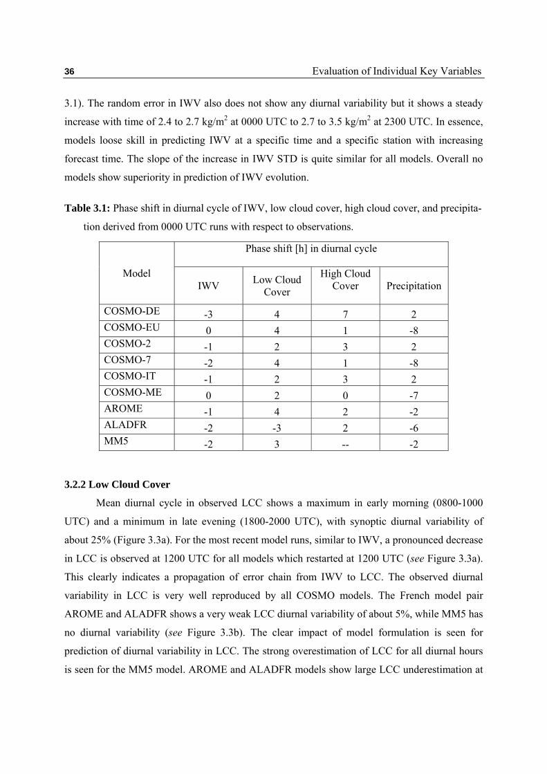
36 Evaluation of Individual Key Variables
3.1). The random error in IWV also does not show any diurnal variability but it shows a steady
increase with time of 2.4 to 2.7 kg/m2 at 0000 UTC to 2.7 to 3.5 kg/m2 at 2300 UTC. In essence,
models loose skill in predicting IWV at a specific time and a specific station with increasing
forecast time. The slope of the increase in IWV STD is quite similar for all models. Overall no
models show superiority in prediction of IWV evolution.
Table 3.1: Phase shift in diurnal cycle of IWV, low cloud cover, high cloud cover, and precipita-
tion derived from 0000 UTC runs with respect to observations.
3.2.2 Low Cloud Cover
Mean diurnal cycle in observed LCC shows a maximum in early morning (0800-1000
UTC) and a minimum in late evening (1800-2000 UTC), with synoptic diurnal variability of
about 25% (Figure 3.3a). For the most recent model runs, similar to IWV, a pronounced decrease
in LCC is observed at 1200 UTC for all models which restarted at 1200 UTC (see Figure 3.3a).
This clearly indicates a propagation of error chain from IWV to LCC. The observed diurnal
variability in LCC is very well reproduced by all COSMO models. The French model pair
AROME and ALADFR shows a very weak LCC diurnal variability of about 5%, while MM5 has
no diurnal variability (see Figure 3.3b). The clear impact of model formulation is seen for
prediction of diurnal variability in LCC. The strong overestimation of LCC for all diurnal hours
is seen for the MM5 model. AROME and ALADFR models show large LCC underestimation at
Model
Phase shift [h] in diurnal cycle
IWV Low Cloud
Cover
High Cloud Cover
Precipitation
COSMO-DE -3 4 7 2 COSMO-EU 0 4 1 -8 COSMO-2 -1 2 3 2 COSMO-7 -2 4 1 -8 COSMO-IT -1 2 3 2 COSMO-ME 0 2 0 -7 AROME -1 4 2 -2 ALADFR -2 -3 2 -6 MM5 -2 3 -- -2

37 Evaluation of Individual Key Variables
0000 to 1800 UTC and quite accurate variability thereafter. All COSMO models slightly overes-
timate the observed LCC diurnal variability for most of the diurnal hours. However, most of
them underestimate observed maxima in LCC, except the COSMO-7 model which shows the
same maxima as in observations. Most of the models predict diurnal maxima in LCC 2 to 4 hours
(Table 3.1) later than observations unlike IWV, except the ALADFR model. LCC diurnal
maxima in ALADFR is seen 3 hours prior to that of observations, which is similar for IWV.
Figure 3.3: Diurnal cycle (summer 2007) in LCC averaged over all stations within the Southern
Germany domain. (a) Most recent model run, (b) 0000 UTC run, (c) Frequency bias of 0000
UTC run on logarithmic scale, and corresponding (d) equitable thread score of 0000 UTC
run. The solid lines denote the HIGHRES models, the corresponding dashed lines represent
their LOWRES counterparts and the filled circles indicate start of new model runs
The frequency bias in LCC also shows stronger diurnal variability for all models with
minimum frequency error during 0800-1000 UTC and maximum frequency error during 1500-
1800 UTC (see Figure 3.3c). We can clearly mark the similarity in systematic error of models

38 Evaluation of Individual Key Variables
with same formulation. The diurnal variability in FBIAS is due to the time lag between the
observed and forecasted LCC. Initially, all COSMO models overestimated the LCC for the first
few forecast hours, followed by a slight underestimation at 0800-1000 UTC, and, thereafter a
common overestimation. The MM5 model consistently overestimates observed frequency, while
AROME and ALADFR underestimated until 1500-1600 UTC and a slight overestimation
thereafter. The random error in LCC (ETS) do not show any diurnal variability with very small
ETS (0.1-0.25) for most of the models, except for MM5 model which shows a large decrease in
ETS after 0600 UTC (see Figure 3.3d). The large decrease in ETS by the MM5 model is linked
with the large overestimation of LCC after 0600 UTC; this overestimation introduces a large
number of false alarms and thus a very small ETS (see Appendix A). HIGHRES models do not
shows superiority over LOWRES models in the prediction of LCC evolution.
3.2.3 High Cloud Cover
Weak diurnal variability is seen in MSG-observed HCC with synoptic variability of about
8% (see Figure 3.4a). For most-recent runs, a pronounced decrease in HCC is seen at 1200 UTC
for all models which restarted at 1200 UTC, except for the MM5 model. This clearly emphasizes
error chain propagation from IWV to HCC, which is similar for LCC. The MM5 model does not
show a pronounced decrease at 1200 UTC which is mostly due to its forecasts of very low
frequency of HCC. Similar to observations, all models also show weak mean diurnal variability
in HCC (see Figure 3.4a). No clear dependency on model formulation on representation of
diurnal variability in HCC is seen. However, all COSMO and French models show large overes-
timation in HCC for all diurnal hours, while the MM5 model shows perfect forecasts at 0 and 3
hours and underestimation thereafter. The large overestimation of COSMO and French models
compared to observations is likely due to optically thin clouds (such as cirrus), which are not
detectable by satellite observation [Wyser and Jones, 2005]. Using MODIS data, Dessler and
Yang [2003] found that 30% of cloud with optical thickness less than 0.05 are undetected by
MODIS instrument. Most of the models overestimate the observed frequency by a factor of 4
(6dB) with very weak diurnal variability (see Figure 3.4c). The diurnal variability in FBIAS is
due to the time lag between the observed and forecasted HCC variability. The MM5 model has
no frequency bias at the first forecast hour; however, the frequency bias increases with forecast
time. This exhibits a clear link with large underestimation of HCC frequency by the MM5 model

39 Evaluation of Individual Key Variables
after 0900 UTC. All models show a very small value of ETS in HCC with weak diurnal variabil-
ity. The MM5 model shows a continuous decrease in forecast skill with forecast time. A clear
trend in ETS is not seen with increasing forecast time for all models. No models show superiori-
ty in the prediction of HCC variability.
Figure 3.4: Diurnal cycle (summer 2007) in HCC averaged over all models grid and MSG grid
cells within the Southern Germany domain. (a) Most recent model run, (b) 0000 UTC run,
(c) Frequency bias of 0000 UTC run on logarithmic scale, and corresponding (d) equitable
thread score of 0000 UTC run. The solid lines denote the HIGHRES models, the corre-
sponding dashed lines represent their LOWRES counterparts and the filled circles indicate
start of new model runs.
3.2.4 Precipitation
Mean diurnal variability in observed precipitation has minima in early morning (0800-1000
UTC) and maxima in late evening (1800-2000 UTC), with a synoptic diurnal variability of about
~0.1mm/h (Figure 3.5a). Similar to other key variables, the precipitation rate also shows a

40 Evaluation of Individual Key Variables
pronounced decrease at 1200 UTC for a model which restarted at 1200 UTC (see Figure 3.5a).
The error introduced in IWV due to assimilation of erroneous radiosounding observations
propagates to LCC, HCC and also in precipitation. This clearly emphasizes a propagation of
error chain in atmospheric water cycle variables. The COSMO-DE model shows an interesting
zig-zag structure in the precipitation diurnal cycle (see Figure 3.5a) which is mostly caused since
it uses latent heat nudging to adjust the precipitation forecast with radar observations. In latent
heat nudging the vertical profile of modeled latent heat release on a specific model grid cell is
scaled according to the difference between the modeled and radar measured precipitation rate
based on an assumed relationship between precipitation formation and latent heat release.
Precipitation rate is overestimated by all models irrespective of model formulation or resolution.
All models have stronger precipitation maxima compared to observations, whereas AROME has
a largest precipitation maximum which is twice as large as observed. This overestimation in
AROME is mostly caused by an overestimated numerical diffusion which induces a too strong
outflow under convective cells [Bauer et al., 2011]. The dominant impact of spin-up effect on
the precipitation rate is seen in all models with large deviation of the precipitation rate from
observations for the first few forecast hours. Such a dominant impact is not observed for other
key variables. All COSMO LOWRES models predicted a diurnal maximum ~8 hours prior to
that of observation, ALADFR predicted 6 hours prior, and MM5 predicted 2 hours prior (see
Table 3.1). Thus, all the LOWRES models predicted diurnal maximum prior to that of observa-
tion, whereas all COSMO HIGHRES models predicted the diurnal maximum 2 hours later to that
of observation except for AROME which predicted it 2 hours prior to the observations.
HIGHRES models shows superiority in prediction of precipitation diurnal variability compared
to their LOWRES counterpart. However, precipitation diurnal variability in HIGHRES models is
not perfect. Guichard et al. [2004] argued that convection occur too early in convection parame-
terized models due to crude triggering criteria and quick onsets of convective precipitation. They
also indicated that the first cloud appearance to precipitation at the ground is delayed by a few
hours in cloud resolving models, whereas this delay is missing in convection parameterized
models. All COSMO LOWRES models have precipitation maxima 2 to 3 hours after the LCC
maxima, whereas maximum precipitation in HIGHRES COSMO models occurred 10 to 11 hours
after the LCC. In contrast to the Guichard et al. [2004] findings, we found a larger difference of
8 hours between maximum in LCC and precipitation for the convection-parameterized MM5
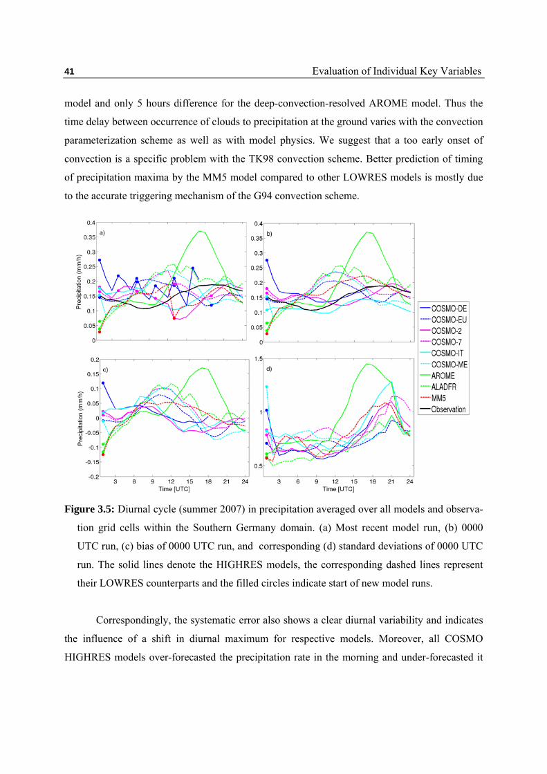
41 Evaluation of Individual Key Variables
model and only 5 hours difference for the deep-convection-resolved AROME model. Thus the
time delay between occurrence of clouds to precipitation at the ground varies with the convection
parameterization scheme as well as with model physics. We suggest that a too early onset of
convection is a specific problem with the TK98 convection scheme. Better prediction of timing
of precipitation maxima by the MM5 model compared to other LOWRES models is mostly due
to the accurate triggering mechanism of the G94 convection scheme.
Figure 3.5: Diurnal cycle (summer 2007) in precipitation averaged over all models and observa-
tion grid cells within the Southern Germany domain. (a) Most recent model run, (b) 0000
UTC run, (c) bias of 0000 UTC run, and corresponding (d) standard deviations of 0000 UTC
run. The solid lines denote the HIGHRES models, the corresponding dashed lines represent
their LOWRES counterparts and the filled circles indicate start of new model runs.
Correspondingly, the systematic error also shows a clear diurnal variability and indicates
the influence of a shift in diurnal maximum for respective models. Moreover, all COSMO
HIGHRES models over-forecasted the precipitation rate in the morning and under-forecasted it

42 Evaluation of Individual Key Variables
after 1000 UTC, except the last few forecast hours. The AROME model over-forecasted the
precipitation rate for all forecast hours except the first few and last forecast hours. All LOWRES
models over-forecasted it during 0600-1600 UTC and under-forecasted it prior and in later
forecast hours. Irrespective to the models formulation and resolution, all models show random
errors one order of magnitude larger than their systematic error. A consistent increase in random
error with forecast time is observed in all models; the slope increase is also quite similar for most
of the models, except the AROME model which has large slope.
3.3 Spatial Distributions in Model Simulations
In order to quantify the model ability in the representation of spatial distribution of the
four key variables, we have analyzed the temporally averaged spatial biases and random errors in
these variables. The spatial map shows Southern Germany domain (see Figure 3.6) and underly-
ing topography is denoted by contour lines.
3.3.1 Integrated Water Vapor
The average models’ biases of hourly IWV compared to the observations are shown in
Figure 3.6 along with the mean observed IWV. Observed IWV shows obvious dependency on
the underlying topography with smaller IWV values for stations located on higher elevation. In
general, high mean IWV values of ~25 kg/m2 are observed for those stations located inside
valleys or plain regions, and for some specific stations the values even exceeded 26 kg/m2,
whereas stations with higher elevations show IWV values smaller than 23 kg/m2. The smallest
IWV value of 8 kg/m2 is observed over the southernmost station in the Northern Alpine foreland
(Zugspitze [47.42N:10.98E:2964m]). The French models AROME and ALADFR have a strong
dry BIAS over most of the stations with the exception of a few stations in the Northern Alpine
foreland which show positive BIAS. The overall large positive BIAS is seen for the MM5 model
over most of the stations, except a few stations which exhibit smaller negative BIAS. All COS-
MO models have small positive BIAS over most of the stations, except a few stations which
have smaller negative BIAS. The LOWRES COSMO models with parameterized convection
have very small biases. The regions of larger and smaller IWV values are well captured by them.
The spatial BIAS structure looks similar for both COSMO-7 and COSMO-ME, in contrast to
COSMO-EU. The major difference between them is their driving model: COSMO-7 and COS-
MO-ME are driven by ECMWF whereas COSMO-EU is driven by GME model. So, the differ-

43 Evaluation of Individual Key Variables
ence in spatial BIAS structure between these models can be due to their driving models. The
deep-convection-permitting COSMO models have large wet biases compared to their corre-
sponding LOWRES counterpart. However, the spatial distribution of their BIAS is quite similar
to that of their LOWRES counterparts. Irrespective of model formulation or resolution, all the
models have a larger bias for the stations located on higher elevations. Also station (Zugspitze)
with the smallest observed IWV value is not captured by any model, which implies even higher
resolution models do not resolve all topographic structures. Most models exhibit similar random
error for IWV, except the MM5 model which has a stronger random error compared to other
models (Figure not shown). All models show stronger random error over stations situated on
higher elevation regions, which clearly emphasize the models’ limitations in prediction of IWV
over complex topography regions. These results also suggest even higher resolution models do
not resolve all topographic structures.
3.3.2 Low Cloud Cover
The average models’ FBIAS of hourly LCC compared to the observations is shown in
Figure 3.7 along with the mean observed LCC. Observed LCC is less than 50% over most of the
stations except for one single station (Deuselbach [49.76N:7.05E:480m]) in the Northwest where
observed LCC is 75% (see Figure 3.7a). This large amount of observed LCC over the Deusel-
bach station may be due instrument error. The western part of the domain has a higher amount of
LCC compared to the eastern parts. The stations in the southern part over the Northern Alpine
foreland have low LCC values. The MM5 model has a large overestimation all over the domain,
while French models AROME and ALADFR have a large underestimation over most of the
stations, except a few stations which show a small overestimation. All COSMO models have
small overestimation over most of the stations, except a few stations which show a small under-
estimation. The COSMO models with parameterized convection have larger FBIAS of 0.5-4 dB
over most of the stations. Overall, all models have larger FBIAS over higher elevation regions.
All convection-permitting COSMO models have comparably smaller FBIAS corresponding to
their LOWRES counterpart. However, COSMO-DE has a smaller FBIAS compared to COSMO-
2 and COSMO-IT models, which may be due their different driving models.
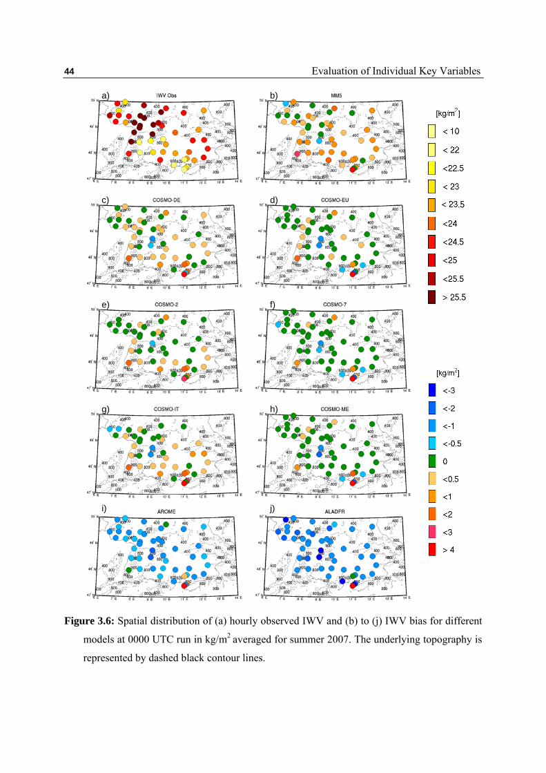
44 Evaluation of Individual Key Variables
Figure 3.6: Spatial distribution of (a) hourly observed IWV and (b) to (j) IWV bias for different
models at 0000 UTC run in kg/m2 averaged for summer 2007. The underlying topography is
represented by dashed black contour lines.
b) a)
c) d)
e) f)
g) h)
i) j)

45 Evaluation of Individual Key Variables
Figure 3.7: Spatial distribution of (a) hourly observed LCC and (b) to (j) LCC frequency bias for
different models at 0000 UTC run in %, averaged for summer 2007. The underlying topog-
raphy is represented by dashed black contour lines.
b) a)
c) d)
e) f)
g) h)
i) j)
[10*log(FBias)]

46 Evaluation of Individual Key Variables
The AROME and ALADFR models have a strong low FBIAS of 0 to 2dB for most of the
stations. Moreover AROME has a small bias compared to its LOWRES counterpart ALADFR.
The MM5 model shows very large FBIAS of 2 to 6 dB over most of the stations. The stations
with higher elevation are clearly marked with stronger frequency biases by all the models.
Overall superiority of HIGHRES models is seen in the prediction of LCC regional distributions
compared to their LOWRES counterpart with comparably smaller frequency biases. Error chain
propagation is clearly seen from IWV to LCC, since most of the stations with IWV dry bias (wet
bias) underestimate (overestimate) the LCC. However, this over or underestimation also depend
upon model resolution. HIGHRES models have a very small FBIAS in LCC over stations with
small IWV BIAS, while LOWRES models exhibit overestimation of LCC over these stations.
Most models exhibit similar random error, except the MM5 model which has a very small ETS
over the entire domain (Figure not shown). All models show small ETS values over stations
situated on higher elevation regions, which clearly emphasize the models’ limitations in predic-
tion of LCC over complex topography regions.
3.3.3 High Cloud Cover
Observed HCC is less than 16% over the entire domain, and a clear influence of under-
ling topography on the HCC amount is seen with stronger values over higher elevation regions
(see Figure 3.8a). The maximum HCC value is observed over the Black forest and northeastern
parts of the domain. Large HCC values over these regions are mainly due to the frequent occur-
rence of convection during summer. The north western parts show the smallest HCC values
which are approximately 10%. MM5 model has a large HCC underestimation over the entire
domain, while COSMO models show overall a large overestimation and AROME and ALADFR
have a small overestimation. Large overestimations by most of the models are likely due to
satellite observations miss optically thin clouds. The regional distribution of FBIAS does not
show any clear dependency on the model resolution. The COSMO-EU model has a larger FBIAS
compared to COSMO-7 and COSMO-ME; this may be due to their different driving models.
COSMO-7 and COSMO-ME models are driven by an ECMWF model whereas COSMO-EU is
driven by the GME model.
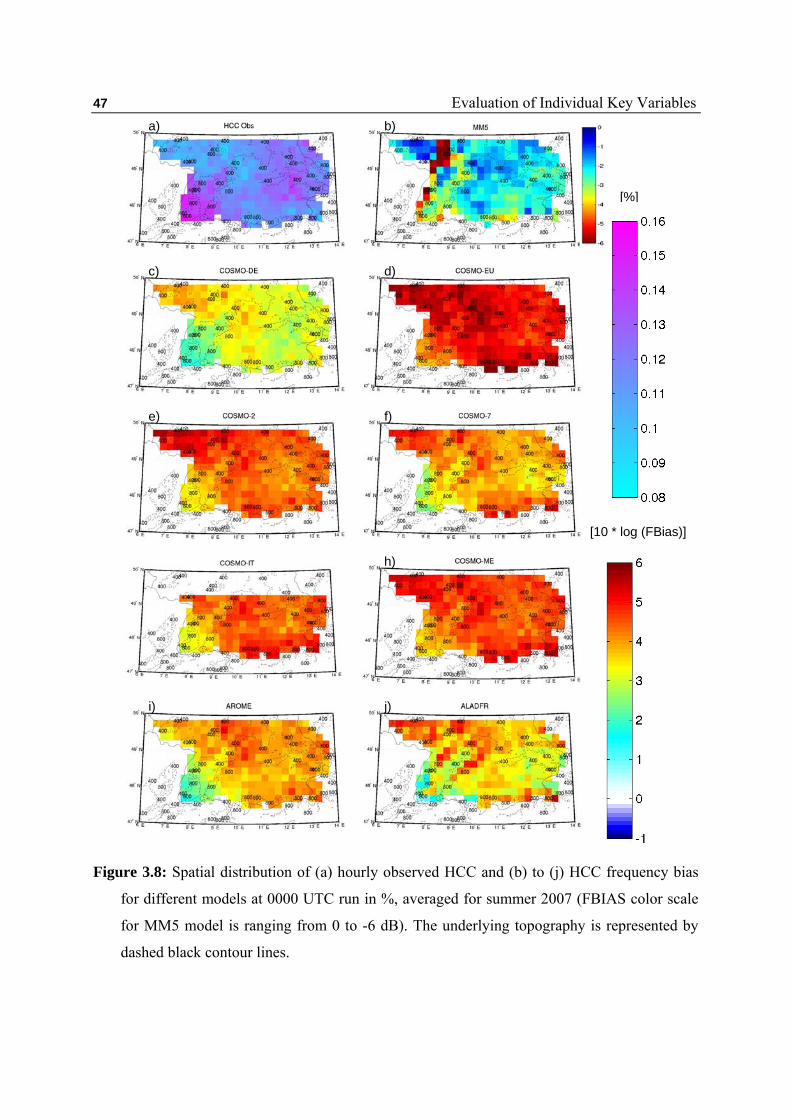
47 Evaluation of Individual Key Variables
Figure 3.8: Spatial distribution of (a) hourly observed HCC and (b) to (j) HCC frequency bias
for different models at 0000 UTC run in %, averaged for summer 2007 (FBIAS color scale
for MM5 model is ranging from 0 to -6 dB). The underlying topography is represented by
dashed black contour lines.
b)
[%]
a)
c) d)
e) f)
h)
j) i)
[10 * log (FBias)]

48 Evaluation of Individual Key Variables
However, COSMO-7 and COSMO-ME also show clear regional differences with larger
overestimation by the COSMO-ME model. Regional discrepancies between these two models
may be due to their different data assimilation methods. COSMO-ME used 3d-Var data assimila-
tion whereas a nudging data assimilation method was used in the COSMO-7 model. The COS-
MO-DE model has the smallest FBIAS compared to all models. COSMO-2 and COSMO-IT
models have a large FBIAS over the entire domain compared to the COSMO-DE model, which
is mostly due to their different driving models. The AROME model has a larger FBIAS com-
pared to its LOWRES counterpart ALADFR model. The MM5 model shows a large underesti-
mation over the entire domain with the largest underestimation of -6dB over the Black forest
region. The smallest FBIAS is seen in the ALADFR model compared to all other LOWRES
models, where the COSMO-DE model has the smallest FBIAS compared to all other HIGHRES
models. The Black forest region is marked by smaller biases for all models producing an overes-
timation of HCC. This clearly implies that models are not very good at accounting for the
topographical influence on the development of HCC, as no models are able to capture the
observed regional difference in HCC.
Most models exhibit similar random error in HCC, except COSMO-DE, COSMO-EU
and MM5 models which show smaller ETS over the entire domain (Figure not shown). However,
all models have small ETS values over higher elevation regions, which clearly emphasize the
models’ limitation in the prediction of HCC over complex topography regions. Small values of
ETS in COSMO-DE and COSMO-EU compared to other COSMO models indicate that initial
conditions dominantly influence the model skill for HCC forecast.
3.3.4 Precipitation
Observed precipitation shows an obvious dependency on the underlying topography, with
the maximum precipitation over the higher elevation regions (see Figure 3.9 a). The highest
hourly precipitation value of 0.35 mm/h is observed in the southern part of the study domain
(Northern Alpine foreland), and a second maximum of 0.25 mm/h is observed in the Black forest
region. Mainly, the northern part of the domain shows the least amount of precipitation, except
for a few higher elevation regions. The LOWRES models overestimated the precipitation amount
over large parts of the domain compared to their corresponding HIGHRES counterparts, except
for the AROME and ALADFR models pair. The AROME and ALADFR models strongly

49 Evaluation of Individual Key Variables
overestimate the precipitation over the entire domain, but the overestimation of the AROME
model is larger compared to the ALADFR model. The LOWRES models particularly have
stronger overestimation of more than 0.1 mm/h over the higher elevation region such as the
Black Forest, Northern Alpine foreland, and the smaller mountains on the northern side. The
correct distribution of precipitation in mountainous terrain is especially challenging for the
models with convection parameterization. Overall, HIGHRES models have smaller differences
compared to observation except for AROME. However, smaller precipitation BIAS is seen for
the LOWRES COSMO-EU model compared to the HIGHRES COSMO-DE models in spatial
and temporal average analysis (Figure 3.1); this is mainly because of the cancellation of large
positive and negative spatial biases. The stronger BIAS over the Northern Alpine foreland and
the Black forest region in all models is probably caused by the poor representation of topography
in the models. Irrespective of their resolution or the driving model or the way convection is
handled, all the models underestimate the precipitation over the northeastern region. Underesti-
mations are smaller for the ALADFR and AROME models, as they have, overall, stronger
overestimation. The COSMO-ME model has smaller regional biases compared to the other two
LOWRES COSMO models. These regional discrepancies are mainly due to the fact that COS-
MO-ME has 3D-Var data assimilation whereas the other two COSMO models use nudging data
assimilation. The smaller discrepancies between COSMO-7 and COSMO-EU may be due to
their different driving models, indicating the influence of the driving model on the regional
precipitation distributions. Convection-permitting HIGHRES COSMO models also have smaller
differences among them in representing the regional precipitation distribution. COSMO-2 and
COSMO-IT models show stronger underestimation in precipitation over the northmost part of
the study domain, whereas such underestimation is not seen for the COSMO-DE model. This
may be due to their different driving models along with COSMO-DE using latent heat nudging
for correction of the precipitation forecast with respect to radar observation.
All COSMO models with parameterized convection have stronger overestimation of pre-
cipitation amount on the windward side of all mountains, and stronger dry bias on the leeward
side. This effect can be seen as stronger biases over the Black forest, the Northern Alpine fore-
land and also over the small mountainous regions. This unrealistic representation of the spatial
pattern of precipitation is referred as the “windward/lee effect” [Wulfmeyer et al., 2008].

50 Evaluation of Individual Key Variables
Figure 3.9: Spatial distribution of (a) hourly observed precipitation and (b) to (j) precipitation
bias for different models at 0000 UTC run in mm/h averaged for Summer 2007. The under-
lying topography is represented by dashed black contour lines.
[mm/h]
[mm/h]
c) d)
f)
h)
i) j)
e)
g)

51 Evaluation of Individual Key Variables
As per Schwitalla et al. [2008], the possible reasons for this effect are (i) inaccurate
simulation of the flow at coarse resolution, and/or (ii) the convection parameterizations cannot
account for cell motion and hydrometeor advection. In reality this effect leads to a substantial
separation between the location where convection is triggered and the area where the rain
reaches the ground. However, ALADFR and MM5 convection-parameterized models do not
have this windward/lee effect. Thus, this effect seems to be affecting the models with the T89
convection parameterization scheme only; the ALADFR and MM5 models didn’t show this
effect as they use the B01 and G94 convection parameterization schemes respectively. Most
models exhibit similar regional distribution of precipitation random error, except the AROME
model which has large random error (Figure not shown). However, all models show stronger
precipitation random error over higher elevation regions, which indicate the models’ limitation in
prediction of precipitation over complex topography regions.
3.4 Verification of Models Skill with Forecast Length
The growth of forecast error with increasing forecast times is evaluated to identify the
dependency of error growth on initial conditions, model formulation, and resolution. The error
growth is calculated as the daily trend in random error. The trend per day in all key variables is
calculated only for 0000 UTC model runs. The analysis is done for various cutoff times starting
with a cutoff of zero and up to 21 hours with interval of 3 hours. The cutoff of 3 hours implies
that the first 3 hours of model forecasts are neglected from analysis (Chapter 2; Section 2.5.1).
Table 3.2 summarizes the mean daily random error and corresponding trend per day for all four
key variables. All HIGHRES models have a smaller trend per day in random error (TDRE) of
IWV corresponding to their LOWRES counterpart.
For all HIGHRES models, TDRE in IWV is smaller than 0.53 kg/m2/day, while for
LOWRES models TDRE ranges from 0.62-0.77 kg/m2/day. The MM5 model has the largest
TDRE of 0.77 kg/m2/day while COSMO-2 has the smallest TDRE of 0.32 kg/m2/day. ALL
models show TDRE smaller than 0.05 ETS in LCC, where the MM5 model has the largest
TDRE of 0.05 ETS and COSMO-ME has the smallest TDRE of 0.01 ETS. Interestingly, the
AROME and ALADFR models have positive TDRE, i.e. an increase of forecast skill with cutoff
hour (As perfect model has ETS =1). TDRE in HCC ranges between 0.02 - 0.07 ETS for all
models. Similar to LCC, TDRE in HCC also do not show any dependence on model formulation

52 Evaluation of Individual Key Variables
or resolution. The TDRE in precipitation for HIGHRES models is nearly twice as large as their
LOWRES counterpart, except for the French models. ALADFR has a larger TDRE than its
LOWRES counterpart AROME. Unlike other COSMO models, COSMO-IT and COSMO-ME
have very small TDRE, although they had similar daily mean STD. This is mostly due to the fact
that they have 3D-Var data assimilation; however, a positive impact of data assimilation is not
seen for IWV and cloud cover. AROME and ALADFR also used 3D-Var data assimilation;
however, a positive impact on forecast skill is not observed for all key variables, which implies
that data assimilation is not the dominant factor compared to model physics. MM5 is the only
model which shows an increase of model skill with forecast time, with negative TDRE. This
might be due to the dry-starting of the MM5 model, which thus needs some time to produce
precipitation, and also may be due to a large spin-up effect. The MM5 model has large TDRE in
IWV, LCC which might be due to the large IWV wet bias and corresponding large overestima-
tion of LCC. Small trend per day in all key variables compared to the mean daily random error
for all models suggest that there is no excessive drying or moistening occurred in the models
themselves through the parameterized precipitation or evaporation fluxes.
Table 3.2: Summary of random errors depicted by Figure 3.1 in terms of daily mean and tem-
poral trend. The random error is expressed by the standard deviation σ for continuous varia-
bles IWV and precipitation and by the equitable thread score ETS for the categorical quanti-
ties LCC and HCC (high resolution models are highlighted).
Model
IWV LCC HCC Precipitation
[kg/m2]
dt
d
[kg/m2/day]
ETS ETS
dt
d
/day
ETS
ETSdt
d
/day
[mm/h]
dt
d
[mm/h/day]
COSMO-DE 2.70 0.53 0.22 -0.03 0.11 -0.07 0.71 0.27
COSMO-EU 2.93 0.72 0.19 -0.02 0.11 -0.03 0.73 0.08
COSMO-2 2.57 0.32 0.22 -0.03 0.14 -0.05 0.78 0.26
COSMO-7 2.92 0.62 0.18 -0.03 0.15 -0.02 0.87 0.08
COSMO-IT 2.83 0.49 0.23 -0.03 0.15 -0.04 0.74 0.04
COSMO-ME 2.86 0.64 0.20 -0.01 0.14 -0.04 0.80 0.01
AROME 2.80 0.46 0.18 0.02 0.15 -0.07 0.99 0.11
ALADFR 2.74 0.62 0.21 0.04 0.15 -0.05 0.71 0.12
MM5_15 3.07 0.77 0.08 -0.05 0.09 -0.06 0.81 -0.03

53
Chapter 4
Multivariate Multi-model Verification
The skill in prediction of individual key variables (IWV, LCC, HCC, and Precipitation) is
assessed in Chapter 3. This classical verification approach is best suited to assess model perfor-
mance in forecasting individual key variables. However, this approach is not very well suited to
identify the reason for model shortcomings. Analyses of similarities among systematic errors of
different key variables give some hints for model shortcomings (Chapter 3). Therefore, the
prospect of analyzing the similarities is elaborated in this chapter by quantifying the similarities
among different models. In detail, the following questions are addressed in this chapter:- Are
there clusters of models revealing the same kinds of error? Are observed similarities between the
different key variables well represented by models? The similarities among different models and
observations for individual key variables are discussed in Section 4.1. Section 4.2 presents the
similarities between systematic errors of different key variables. The similarities of these varia-
bles between models and observations are explored in Section 4.3. Section 4.4 assesses the
similarities between model key variables and observations for different time lags.
4.1 Similarities among Variables
The clusters of models for specific factor such as model formulation, resolution, and driv-
ing model may help in identifying factors responsible for model shortcomings. The similarities
are quantified by means of linear statistical relationships. Most of the key variables evaluated in
this study are non-Gaussian distributed. Thus linear relationships among them are assessed by
Spearman’s rank correlation which is a nonparametric measure of linear and non-linear mono-
tonic association. Spearman’s rank correlation is not sensitive to non-Gaussian distributed data
like product-moment correlation. Spearman’s rank correlation is simply the product-moment
correlation coefficient of the ranks of the data [Wilks, 1995]. As the rank of data is used instead
of the data itself, rank correlation is less sensitive to large outlier values compared to product-
moment correlation. The rank correlations are calculated over each station for IWV and LCC and
over each grid cell for HCC and precipitation over the whole study domain for 0000 UTC
models run only. The significance of rank correlation is assessed by bootstrap resampling
methods using 95% and 5% quantiles of 1000 bootstrap samples (see Appendix B).
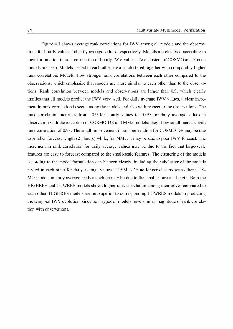
54 Multivariate Multimodel Verification
Figure 4.1 shows average rank correlations for IWV among all models and the observa-
tions for hourly values and daily average values, respectively. Models are clustered according to
their formulation in rank correlation of hourly IWV values. Two clusters of COSMO and French
models are seen. Models nested in each other are also clustered together with comparably higher
rank correlation. Models show stronger rank correlations between each other compared to the
observations, which emphasize that models are more similar to each other than to the observa-
tions. Rank correlation between models and observations are larger than 0.9, which clearly
implies that all models predict the IWV very well. For daily average IWV values, a clear incre-
ment in rank correlation is seen among the models and also with respect to the observations. The
rank correlation increases from ~0.9 for hourly values to ~0.95 for daily average values in
observation with the exception of COSMO-DE and MM5 models: they show small increase with
rank correlation of 0.93. The small improvement in rank correlation for COSMO-DE may be due
to smaller forecast length (21 hours) while, for MM5, it may be due to poor IWV forecast. The
increment in rank correlation for daily average values may be due to the fact that large-scale
features are easy to forecast compared to the small-scale features. The clustering of the models
according to the model formulation can be seen clearly, including the subcluster of the models
nested in each other for daily average values. COSMO-DE no longer clusters with other COS-
MO models in daily average analysis, which may be due to the smaller forecast length. Both the
HIGHRES and LOWRES models shows higher rank correlation among themselves compared to
each other. HIGHRES models are not superior to corresponding LOWRES models in predicting
the temporal IWV evolution, since both types of models have similar magnitude of rank correla-
tion with observations.

55 Multivariate Multimodel Verification
Figure 4.1: Rank correlation of IWV over all stations within the study domain for summer 2007
(a) hourly value (b) daily forecast average.
a)
b)

56 Multivariate Multimodel Verification
For IWV, model formulation is the dominant factor causing models to cluster together.
Figure 4.2 depicts the rank correlation for LCC among models along with the observations for
hourly values and daily average values. No clustering of models with model physics, resolution,
driving model, or the models nested in each other is seen. The rank correlation among the models
as well as with respect to observations is smaller than that for IWV. The smaller rank correlation
of 0.52 to 0.61 between the models and the observations for hourly LCC values denotes model
limitations in the prediction of low cloud cover. For daily average LCC values, a clear increment
in rank correlation is seen for all models and also with respect to the observations. The increment
in rank correlation for daily average values is mainly due to averaging out diurnal discrepancies,
though it may also due to the large-scale cloud structures, which are easy to forecast compared
to the individual clouds. The rank correlation increases from 0.52-0.61 for hourly values to 0.59-
0.66 for daily values with respect to observations. The clustering of models according to their
model formulation is seen. However, no clear clustering among the models nested in each other
is seen except for the COSMO-IT and COSMO-ME pair and French models pair. The HIGHRES
models show better rank correlation with observations compared to the corresponding LOWRES
models. Similar to the IWV, models with the same resolution show higher rank correlation
among themselves. Models are clustered together according to model formulation in LCC,
similar to IWV. However, unlike in IWV, HIGHRES models show a slightly stronger rank
correlation with the observations. Model formulation is the dominant factor for models to cluster
together in LCC.
The rank correlation for HCC in all the models and observations for hourly values and
daily average values are shown in Figure 4.3. Clustering of models according to their model
formulation is seen except for COSMO-DE and COSMO-EU models. COSMO-DE and COS-
MO-EU models differ from other COSMO models by their driving model. COSMO-DE and
COSMO-EU models are driven by the GME global models, while other COSMO models are
driven by the IFS (ECMWF) model. Thus driving models show a dominant impact on the
prediction of HCC. Clusters of models nested in each other are seen for most of the models pairs,
except for the COSMO-DE and COSMO-EU models.
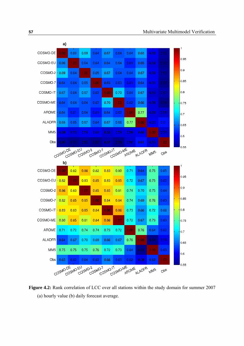
57 Multivariate Multimodel Verification
Figure 4.2: Rank correlation of LCC over all stations within the study domain for summer 2007
(a) hourly value (b) daily forecast average.
a)
b)
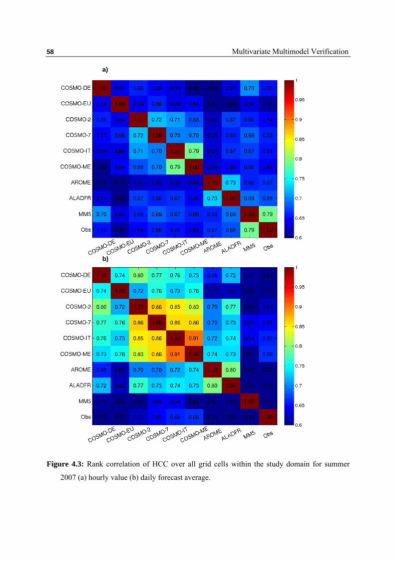
58 Multivariate Multimodel Verification
Figure 4.3: Rank correlation of HCC over all grid cells within the study domain for summer
2007 (a) hourly value (b) daily forecast average.
a)
b)

59 Multivariate Multimodel Verification
The rank correlation among the models is not significantly higher than with observations,
unlike what is seen for IWV and LCC, which implies models are not as similar to each other
compared to the observations. No clear improvement of HIGHRES models over their corre-
sponding LOWRES models is seen. For daily average HCC, rank correlation among the models
increases significantly; however, rank correlations decrease between models and observations.
This decrease of rank correlation for daily forecasts is not observed for IWV and LCC. Decrease
of rank correlation between models and observations may be due to the very poor forecasts of
HCC. However, this is contradictory to the fact that large-scale cloud structure is easy to forecast
compared to individual clouds. The MM5 model shows the largest rank correlation for hourly
values compared to other models, but has the smallest rank correlation for the daily average
values. This may be due to the best representation of diurnal variability of observed HCC by the
MM5 model compared to the other models. The COSMO models driven by the IFS (ECMWF)
model have a higher rank correlation with the observations compared to other COSMO models
as well as the rest of the models. The HIGHRES models do not show any clear improvement
over the LOWRES models. For HCC the clear impact of driving models on clustering is seen
along with model formulation.
Rank correlation among models and observations for precipitation is depicted in Figure
4.4 for hourly values and daily average values. The clustering of models according to their model
formulation and resolution is seen, while no clustering is seen among models nested in each
other. As summer precipitation is dominated by convective rain, clustering of the models accord-
ing to model resolution is more dominant, as convection is treated differently in HIGHRES and
LOWRES models. The deep convection is explicitly represented in HIGHRES models, while it
is parameterized in LOWRES models. The HIGHRES models show comparably larger rank
correlation with observations compared to their corresponding LOWRES counterpart for hourly
precipitation. The rank correlation among models is not larger than that with observation except
for the COSMO models, which implies that only COSMO models are similar to each other.
Clear improvement of rank correlation for daily average values is seen, but improvement of
HIGHRES models over the LOWRES models is no longer seen.

60 Multivariate Multimodel Verification
Figure 4.4: Rank correlation of precipitation over all grid cells within the study domain for
summer 2007 (a) hourly value (b) daily forecast average.
a)
b)

61 Multivariate Multimodel Verification
This implies that HIGHRES models better represent the observed diurnal variability
compared to corresponding LOWRES models; however, no improvement is conclusive in the
total amount of precipitation. For precipitation, model resolution is a dominant factor for the
models to cluster together.
4.2 Similarities between Errors of Different Key Variables
Precipitation is the final component of a process chain; thus, error in one key variable
should be propagated to other variables. In this section we explore whether it is possible to detect
any error chain by assessing error correlation between different variables. Assessment of similar-
ities between the biases of different key variables showed a propagation of error from IWV to
LCC; however, further propagation of error to other variables is not seen (see Section 3.5,
Chapter 3). Assessments of error correlation between different key variables are difficult due to
their different observational locations. To overcome this issue the study domain is divided into
six subdomains. The choice of subdomain is made in a way so that at least three observation
stations for each key variable are inside every subdomain (see Figure 4.5). Error in continuous
variables (IWV and precipitation) is represented by bias, while for categorical variables (LCC
and HCC) error is represented by frequency bias. The significant difference between rank
correlations of different models or observations are tested by a rank sum test and also by a
bootstrap resampling method with 1000 bootstrap samples (see Appendix B).
The rank correlations between subdomain-averaged biases of all key variables for sum-
mer 2007 are depicted in Figure 4.6. Rank correlation between IWV and LCC biases is very
small for most of the models except for the French models. Most of the models don’t even have
significant rank correlation except for the French models. No clusters of models according to
model physics, resolution, or driving model are seen. The MM5 model shows the lowest rank
correlation with value close to zero. IWV and HCC biases also have small rank correlation
values; however, rank correlations are significant for all models. The MM5 model shows the
largest rank correlation of 0.35, while all other models have correlations smaller than 0.25.
Similar to rank correlation between IWV and LCC biases, no clustering of models is found for
rank correlation between IWV and HCC biases. Rank correlations between IWV and precipita-
tion biases are less than 0.25 for most of the models, except for the COSMO-IT and the MM5
model. COSMO-IT and MM5 show a rank correlation of 0.3 and 0.35, respectively. Clusters of
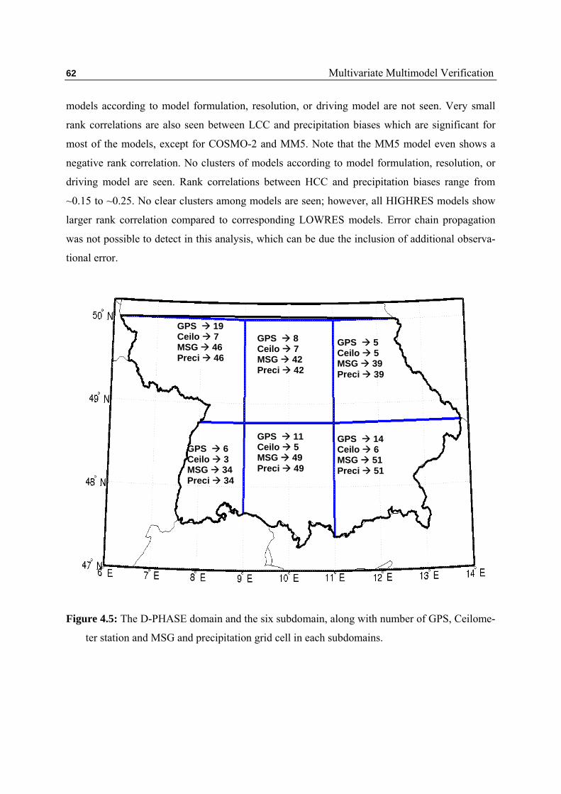
62 Multivariate Multimodel Verification
models according to model formulation, resolution, or driving model are not seen. Very small
rank correlations are also seen between LCC and precipitation biases which are significant for
most of the models, except for COSMO-2 and MM5. Note that the MM5 model even shows a
negative rank correlation. No clusters of models according to model formulation, resolution, or
driving model are seen. Rank correlations between HCC and precipitation biases range from
~0.15 to ~0.25. No clear clusters among models are seen; however, all HIGHRES models show
larger rank correlation compared to corresponding LOWRES models. Error chain propagation
was not possible to detect in this analysis, which can be due the inclusion of additional observa-
tional error.
Figure 4.5: The D-PHASE domain and the six subdomain, along with number of GPS, Ceilome-
ter station and MSG and precipitation grid cell in each subdomains.
GPS 19 Ceilo 7 MSG 46 Preci 46
GPS 8 Ceilo 7 MSG 42 Preci 42
GPS 5 Ceilo 5 MSG 39 Preci 39
GPS 6 Ceilo 3 MSG 34 Preci 34
GPS 11 Ceilo 5 MSG 49 Preci 49
GPS 14 Ceilo 6 MSG 51 Preci 51

63 Multivariate Multimodel Verification
Figure 4.6: The rank correlation for the systematic error of sub-domain averaged (a) IWV and
LCC, (b) IWV and HCC, (c) IWV and precipitation, (d) LCC and precipitation, and (e) HCC
and precipitation for summer 2007, Error bars denote the inter-quantile distance between
95% and 5% quantile from bootstrapping distribution, HIGHRES models denoted by green
bars and LOWRES models by red bars.
a) b)
c) d)
e)

64 Multivariate Multimodel Verification
4.3 Similarities between Different Key Variables
Propagation of errors in key variables absolute values was not found in the error correla-
tion analysis. Thus, another approach of assessing the strength of relationships between different
key variables in observations and models is proposed. This approach might be a new verification
technique to diagnose model shortcomings. The strength of relationships is assessed by mean of
rank correlation. Most of the earlier research activities were focused on relations between water
vapour and precipitation. Many researchers extensively studied the relationship between column-
integrated water vapour and precipitation over the tropics using observations [Back et al., 2010;
Holloway and Neelin, 2010; Sherwood et al., 2004] and also using cloud-resolving models
[Tompkins, 2001; Grabowski, 2003]. Studies by Zhang and Wang [2006] and Bechtold et al.
[2008] shown that the strength of this relationship is not well represented in global models. Very
few such studies are available over midlatitudes. Van Baelen et al. [2011] investigated the water
vapour distribution and its relationship with the evolution of precipitation systems over the
COPS region using GPS 2D and 3D tomography and ground based weather radar. They found a
predominant role of water vapour as a precursor to a local convective initiation. However, this
study is limited to a few numbers of cases and the main goal of this study was to better under-
stand the role of water vapour for convection initiation.
The rank correlations among the subdomain averaged key variables for summer 2007 in
the models and observations are depicted in Figure 4.7. The significance of result is tested by the
mean of the rank sum test and also by the bootstrap resampling method (see Appendix B). Weak
linear relationships between observed IWV and LCC are found with a rank correlation of ~0.2.
Observed IWV has a stronger linear relationship with HCC compared to LCC, with a rank
correlation of 0.4. A rank correlation of 0.35 is seen between IWV and precipitation, which is
comparably smaller than the correlation between IWV and HCC. A rank correlation of 0.43 is
seen between LCC and precipitation, and implies a stronger linear association. The strongest
linear relationship observed between HCC and precipitation with rank correlation of 0.54. The
weak linear association between IWV and LCC might be due to the fact that formation of low
clouds is initiated with the condensation of water vapour. Thus, an increase of low clouds is
associated with a decrease of IWV, which is also seen in diurnal variability (Section 3.2 Chapter
3). Formation of precipitation subsequently increases the high clouds (anvil formation) and
atmospheric water vapour. As the increase of HCC and IWV occurs nearly at the same time as

65 Multivariate Multimodel Verification
precipitation formation, a stronger relationship is found between them. However, a comparably
weak relationship is seen between IWV and precipitation, which may be due to the time delay
between precipitation formation and the increase of IWV. A stronger relationship is seen be-
tween LCC and precipitation as the formation of low clouds incites subsequent precipitation, but
with certain time delay. A very strong linear relationship is seen between HCC and precipitation,
as the formation of precipitation incites subsequent high clouds.
The observed strength of the relationship between IWV and LCC (see Figure 4.7a) is un-
derestimated by most of the models with significantly smaller rank correlation of 0.15-0.18,
except by French models. Significant overestimation of relationship strength is shown by the
AROME and ALADFR models with rank correlations of 0.20 and 0.30, respectively, and implies
that model clouds appear for less water vapour. The MM5 model shows a similar strength of
linear relationship as in the observations with rank correlation of 0.18, which implies the best
representation of the relationship between low clouds and water vapour. HIGHRES models do
not better represent the observed strength of the linear relationship compared to LOWRES
models. Most of the models quite well represent the observed relationship between IWV and
HCC (see Figure 4.7b) with slight under and overestimation. Most of the HIGHRES models
slightly underestimate the strength of the observed relationship with rank correlation of ~0.35
while LOWRES models overestimate with rank correlation of 0.42-0.48, except for the French
model pair. MM5 and AROME models show a comparably stronger overestimation of the
observed relationship. The observed strength of the relationship between IWV and precipitation
(see Figure 4.7c) is also quite well represented by most of the models with slight under- and
overestimation. Most of the LOWRES models overestimate the observed strength of the relation-
ship (rank correlation 0.35-0.48), except the COSMO-7 model. The slight underestimation of the
relationship strength is seen in the COSMO-7 model (rank correlation 0.31), while the MM5
model shows the largest overestimation with a rank correlation of 0.48. All HIGHRES models
underestimate the observed strength of the relationship with rank correlation of ~0.28-0.30.
The strength of linear relationship between LCC and precipitation (see Figure 4.7d) is
overestimated by all models with rank correlation of 0.55-0.68. This clearly emphasizes a
stronger dependency of model precipitation on LCC. Most of the HIGHRES models show less
overestimation compared to the corresponding LOWRES models, except the French model pair,
where AROME has a larger overestimation compared to the corresponding LOWRES model
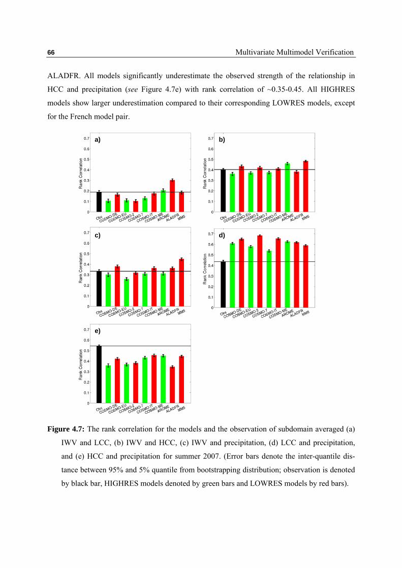
66 Multivariate Multimodel Verification
ALADFR. All models significantly underestimate the observed strength of the relationship in
HCC and precipitation (see Figure 4.7e) with rank correlation of ~0.35-0.45. All HIGHRES
models show larger underestimation compared to their corresponding LOWRES models, except
for the French model pair.
Figure 4.7: The rank correlation for the models and the observation of subdomain averaged (a)
IWV and LCC, (b) IWV and HCC, (c) IWV and precipitation, (d) LCC and precipitation,
and (e) HCC and precipitation for summer 2007. (Error bars denote the inter-quantile dis-
tance between 95% and 5% quantile from bootstrapping distribution; observation is denoted
by black bar, HIGHRES models denoted by green bars and LOWRES models by red bars).
a) b)
c) d)
e)
67 Multivariate Multimodel Verification
4.4 Similarities between Different Key Variables for Different Lag-times
Most of the atmospheric water cycle processes occur with some time delay between
them. Thus, the maximum relationship strength between key variables can be achieved at a
specific time lag. The approach of assessing relationships between different key variables in
models and observations is extended for different lag times. This will help to highlight the
observed time difference between the atmospheric water cycle processes and how it is represent-
ed in models.
The time-lag relationship among the different key variables is assessed for the ± 48 hour
lag time. Table 4.1 shows the summary of the largest rank correlation achieved and correspond-
ing lag time along with the rank correlation at the 0-lag hour. Observed IWV has the largest rank
correlation of 0.30 with the LCC at -9 hour lag which is significantly larger than correlation at 0-
lag hours. In other words, IWV has the largest linear relationship with the LCC nine hours
earlier. The largest relationship between IWV and HCC is found at a one-hour lag time, which is
in fact not significantly different from correlation at 0-lag hours. The largest rank correlation of
0.37 between observed IWV and precipitation is observed at -2 hours lag time, which is signifi-
cantly larger than the rank correlation at 0-lag hours. Observed LCC shows the largest rank
correlation of 0.45 with the precipitation which occurs 6 hours later, which is significantly larger
than correlation at 0-lag hours. HCC shows the largest rank correlation with precipitation one
hour earlier, which is not significantly larger than the rank correlation at 0-lag hours.
The lag of the largest correlation in IWV and LCC is quite well represented by most of
the models with difference of 1-2 hours, except by the French model pair. AROME and
ALADFR show the largest rank correlation at -5 and -3 lag hours respectively. A very small lag
delay between IWV and LCC in French models suggests the misrepresentation of IWV and LCC
relationship. As seen for 0-hour lag analysis, the relationship strength between IWV and LCC is
underestimated by most of the models except by the French models. All models show the largest
rank correlation between IWV and HCC at 0 to 2 hour lag; however, it is not significantly
different than the rank correlation at 0-lag hours. Thus IWV and HCC have the largest relation-
ship at 0-lag hours, which is very well reproduced by all models. No difference between
HIGHRES and LOWRES models is seen to represent the lag relationship between IWV and
HCC. The ranking of models for relationship strength between IWV and HCC is same as in 0-
hour lag analysis (Section 4.4). Most of the models very well reproduced the observed delay of -

68 Multivariate Multimodel Verification
2 hour between IWV and precipitation, except ALADFR which shows delay of -1 hour. The
ranking of models for relationship strength between IWV and precipitation is same as in 0-hour
lag analysis. All HIGHRES COSMO and MM5 models show a largest rank correlation between
LCC and precipitation at 2 hour lag, whereas COSMO LOWRES and French model show a
largest rank correlation at the 0 lag. In fact the observed delay of 6 hours between LCC and
precipitation is not reproduced by any of the models. This suggests a problem in the representa-
tion of the relationship between LCC and precipitation in all models. Models show the same
ranking as in 0 -hour lag analysis for the relationship strength between LCC and precipitation.
The lag of the largest rank correlation between HCC and precipitation is not represented by most
of the models, except COSMO-ME and the French models. This result emphasizes the problem
of representing the HCC-precipitation relationship in models. Models show the same ranking as
in 0-hour lag analysis for relationship strength between HCC and precipitation.
Another attempt is made to asses the dependency of the relationship strength between dif-
ferent key variables on topographical characteristics. The relationships between different key
variables over different subdomains are evaluated (Figure not shown). The clear impact of the
number of observational stations in individual subdomains on rank correlation is seen instead of
domain topographical characteristics. Subdomains with more stations show a stronger relation-
ship between different key variables compared to subdomains with less stations. These results
suggest the gridded observations of IWV and LCC will be very useful to assess linear relation-
ships between different key variables, which will ultimately help to reveal model shortcomings
in corresponding atmospheric processes.

69 Multivariate Multimodel Verification

70 Multivariate Multimodel Verification

71
Chapter 5
Evaluation of Integrated Water Vapor, Cloud Cover and Precipitation
Predicted by Ensemble Systems
This chapter is dedicated to evaluate the performance of ensemble prediction system
with respect to the prediction of integrated water vapor, cloud cover and precipitation. More
precisely, this chapter addresses the following questions: Do the ensemble prediction systems
reflect the uncertainty in forecasting the key variables? Is their performance similar? How
reliable is a multi-model EPS? What is the primary perturbation affecting the EPS perfor-
mance, the initial conditions or the model physics? Further, the quality of ensemble forecast-
ing systems is verified for complete probability density functions as well as for five thresh-
olds for reliability, resolution, sharpness and skill attributes of ensemble forecasts. This
chapter is organized as follows. Section 5.1 illustrates the performance of the individual
ensemble members as well as the ensemble means for prediction of IWV and precipitation.
Representation of forecast uncertainty in the prediction of IWV and precipitation by the
ensemble forecasting systems is evaluated in Section 5.2. The performance of probability
forecasts for all key variables from all ensemble systems is described in Section 5.3 for all the
probability density functions as well as for different thresholds.
5.1 Performance of Individual Ensemble Members and Ensemble Mean Forecast
Since we intend to evaluate the complete probability density function of each key var-
iable, the categorical variables such as LCC and HCC are limited to certain verification
methods. The verification of LCC and HCC is done only for categorical verification of a 50%
threshold. The ensemble prediction systems provide the forecast for each three-hour period,
so the observational data for IWV, LCC and HCC closest to every third clock hour are
considered. However, the precipitation observations are accumulated every three hours as in
the EPS. All key variables of the atmospheric water cycle predicted by CLEPS, CSREPS,
PEPS and LAMEPSAT (see Section 2.3) ensemble prediction systems are verified over the
whole study domain for summer 2007. However, the LAMEPSAT ensemble prediction
system does not provide the forecast for IWV (Chapter 2), thus only the three remaining
ensemble systems are verified for IWV. Verification statistics are calculated over the contin-
uous time series of all stations or grid cells within a verification domain for the whole time
period.
72 Evaluation of Ensemble Prediction Systems
All ensemble members are considered to have very small long-term statistical differ-
ences, as the ensemble method assumes an equally likely occurrence for individual members.
The equally likely test for ensemble members is very useful to find problems in the perturba-
tion method, as a large perturbation leads to very large differences in long-term statistics.
This section examines the performance of each individual ensemble member and also the
superiority of the ensemble mean over the individual ensemble members, which also helps to
diagnose equally likely occurrences within individual ensemble members.
Previous studies by Du et al. [1997] and Ebert [2001] showed the superiority of the
ensemble mean for precipitation forecast over individual ensemble members. The ensemble
mean is more skillful due to the cancellation of discrepancies among the members, and only
common features remain during the process of ensemble averaging. Many researchers have
proposed distinct methods to produce more accurate deterministic ensemble forecasts. A few
studies such as Van den Dool and Rukhovets [1994] and Krishnamurti et al. [1999, 2000]
used a weighted-averaging method to derive deterministic forecasts. In this method, the
ensemble forecasts are optimally weighted according to their skill. Xie and Arkin [1996] and
Huffman et al. [1997] used the inverse of the expected error variance to produce a determinis-
tic forecast. Ebert [2001] recommended a probability matching approach which is based on
setting the probability distribution function (PDF) of the less accurate data equal to that of the
more accurate data, which she claimed produces the most skillful deterministic forecasts from
the EPS compared to other methods. In this study our aim is to verify the relative perfor-
mance of the different ensemble systems instead of improving the deterministic forecasts
from the ensembles. So we chose the relatively simpler arithmetic mean to derive the deter-
ministic forecast from the EPS. The reader should be aware that, for a single-model based
ensemble system, ensemble averaging can remove random errors but not a systematic bias.
However, for a multi-model and/or multi-physics ensemble, bias could also be reduced. We
are intercomparing single-model ensemble systems (CLEPS, CSREPS, and LAMEPSAT)
with the multimodel EPS (PEPS, Chapter 2 Section2.3.2), and hence the standard deviation
(STD) is considered as a skill score for comparison instead of the root-mean-square, as the
latter one is a blend of random and systematic error. To better understand the performance of
ensemble prediction systems, the BIAS of individual ensemble members also given along
with the STD. Figure 5.1 depicts the BIAS and STD in IWV for individual members of
different ensemble systems and the corresponding ensemble mean. All three ensemble
systems show significant decrease of random error in IWV for the ensemble mean compared
to individual members.

73 Evaluation of Ensemble Prediction Systems
Figure 5.1: Bias (green bars) and standard deviation (orange bars) in IWV over the Southern
Germany study domain for summer 2007 for individual members of (a) CLEPS, (b)
CSREPS, and (c) PEPS.
Moreover, PEPS stands superior to other ensemble prediction systems with smaller
random error in the ensemble mean. The random error in CLEPS ensemble members roughly
varies between 3.4 to 4.2 kg/m2 with small discrepancies in different members, and is re-
duced to 3 kg/m2 for the ensemble mean. The random error of individual ensemble members
of CSREPS varies from 3.4 kg/m2 to 3.8 kg/m2, and is reduced to 3.1 kg/m2 for the ensemble
mean. As shown in Figure 5.1b, it is worth noting that each set of four ensemble members are
similar compared to other members for both biases and STD, which indicates the clear impact
of initial conditions from the four global models providing lateral forcing data. The random
error for almost all individual members of PEPS is smaller compared to members of CLEPS
and CSREPS. The random error for the ensemble mean in PEPS is also reduced to 2.4 kg/m2
and is significantly smaller than that for other ensemble members. Overall, CLEPS exhibits
small IWV wet biases except for first two ensemble members, while CSREPS has a small dry
bias for all ensemble members. Most of the ensemble members of PEPS exhibit an IWV wet
bias, while two ensemble members have a large dry bias. CLEPS and CSREPS are COSMO-
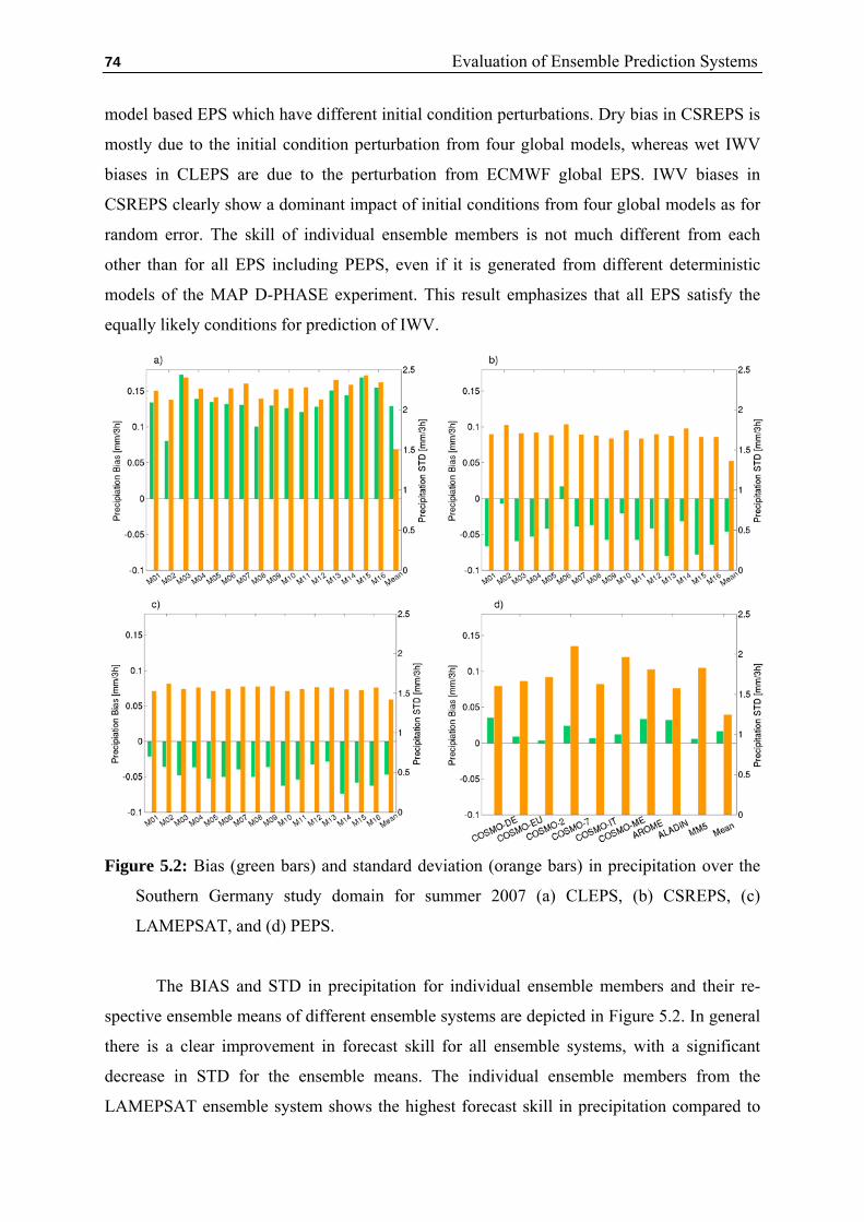
74 Evaluation of Ensemble Prediction Systems
model based EPS which have different initial condition perturbations. Dry bias in CSREPS is
mostly due to the initial condition perturbation from four global models, whereas wet IWV
biases in CLEPS are due to the perturbation from ECMWF global EPS. IWV biases in
CSREPS clearly show a dominant impact of initial conditions from four global models as for
random error. The skill of individual ensemble members is not much different from each
other than for all EPS including PEPS, even if it is generated from different deterministic
models of the MAP D-PHASE experiment. This result emphasizes that all EPS satisfy the
equally likely conditions for prediction of IWV.
Figure 5.2: Bias (green bars) and standard deviation (orange bars) in precipitation over the
Southern Germany study domain for summer 2007 (a) CLEPS, (b) CSREPS, (c)
LAMEPSAT, and (d) PEPS.
The BIAS and STD in precipitation for individual ensemble members and their re-
spective ensemble means of different ensemble systems are depicted in Figure 5.2. In general
there is a clear improvement in forecast skill for all ensemble systems, with a significant
decrease in STD for the ensemble means. The individual ensemble members from the
LAMEPSAT ensemble system shows the highest forecast skill in precipitation compared to

75 Evaluation of Ensemble Prediction Systems
other ensemble systems, which is likely due to the slightly larger negative BIAS in
LAMEPSAT (Figure 5.2c). The random error for the individual CLEPS ensemble members
ranges from 2.2 to 2.4 mm/3h with slight differences among the members, but for the ensem-
ble mean it is further reduced to 1.5 mm/3h. Similarly, for CSREPS the random error varies
from 1.7 to 1.9 mm/3h individually, and is reduced to 1.4 mm/3h for their mean.
LAMEPSAT showed a STD of 1.55 to 1.65 mm/3h for the individual members. Again for the
ensemble mean an improvement, with a smaller STD of 1.3 mm/3h, is observed. The random
error in PEPS is between 1.55 and 2.2 mm/3h for individual members, and reduces to 1.25
mm/3h for the mean. CLEPS exhibits a large positive bias for all ensemble members while
CSREPS and LAMEPSAT have large negative biases, and PEPS has smaller positive biases.
On average, the performance of the individual members of respective ensemble sys-
tems is quite similar except for PEPS, of which the members show large differences among
them. This large difference in PEPS’s ensemble members is mainly due to the different
treatment of convection in the models: some have parameterized convection while the others
calculate the convection explicitly. This result clearly implies that, except for PEPS, all other
EPS satisfy equally likely conditions for prediction of precipitation.
5.2 Representation of Forecast Uncertainty – An Assessment
For a perfect ensemble system, in the sense that it accurately accounts for all sources
of forecast uncertainty, the observation should be indistinguishable from the forecast of
ensemble members [Anderson, 1996; Hamill, 2001]. The spread of a perfect ensemble
forecasting system provides information about the forecast uncertainty. The large ensemble
spread is associated with large forecast uncertainty, and small spread is associated with small
forecast uncertainty. The representation of forecast uncertainty by CLEPS, CSREPS,
LAMEPSAT, and PEPS is analyzed in this section by the spread / skill relationship as well as
by rank histogram. The ensemble spread is calculated as a standard deviation of individual
ensemble forecasts from their mean [Zhu, 2005; Appendix A.6] while, ensemble error
(RMSE) is the distance measured from the ensemble mean to the observation. Grimit and
Mass [2007] suggest that, for perfect EPS, error and ensemble spreads should be positively
correlated on average, as ensemble error will be equal to spread. Thus, to support the spread
skill relationship, we also verified their correlation.
All EPS show a large increase in ensemble error with lead time for IWV forecasts
(Figure 5.3a). PEPS shows the least error and CSREPS shows the largest error compared to
the rest. For the initial lead time, all the EPS exhibit larger errors compared to the spread,

76 Evaluation of Ensemble Prediction Systems
suggesting all possible forecast uncertainties are not represented by them (underdispersive).
PEPS well represents the forecast uncertainty with smaller underdispersion (spread close to
the error), whereas CSREPS is most underdispersive. CLEPS represents a reasonable forecast
uncertainty after 36-hour lead time. For most of the ensemble systems, the difference be-
tween the ensemble spread and the error increases with lead time, indicating the EPS are
becoming more and more underdispersive with lead time. However for CLEPS, the differ-
ence between spread and error decreases up to 36 hours lead time and thereafter becomes
slightly overdispersive with quite good agreement between spread and error. This shows
CLEPS has good skill for medium-range forecasts. Additionally, the correlation between the
ensemble spread and the error is calculated over each station for the study period to support
this result. CLEPS and CSREPS have the lowest correlation of below 0.1 (Table 5.1): for
CSREPS, the correlation is small and negative; however, for PEPS a correlation of 0.55 is
observed between the ensemble spread and the error. In sum, the correlation for all ensemble
systems decreased with lead time. This emphasizes multimodel multi-analysis EPS (PEPS)
can account most of the forecast uncertainty compared to single-model EPS for IWV fore-
casts.
Figure 5.3: Spread and error (RMSE) as function of lead time in (a) IWV [kg/m2] and (b)
precipitation [mm/3h] over the Southern Germany study domain for summer 2007. (solid
line denotes the spread and dotted line denotes the error)
The evolution of the spread / skill relationship with lead time for precipitation is de-
picted in Figure 5.3b. The error (RMSE) in precipitation for CSREPS, PEPS and
LAMEPSAT is slightly increasing with lead time. For CLEPS the error in precipitation
decreases with lead time up to 30 hours lead time and increasing thereafter. The initial
decrease of precipitation error in CLEPS is mostly due to the larger scale ensemble perturba-
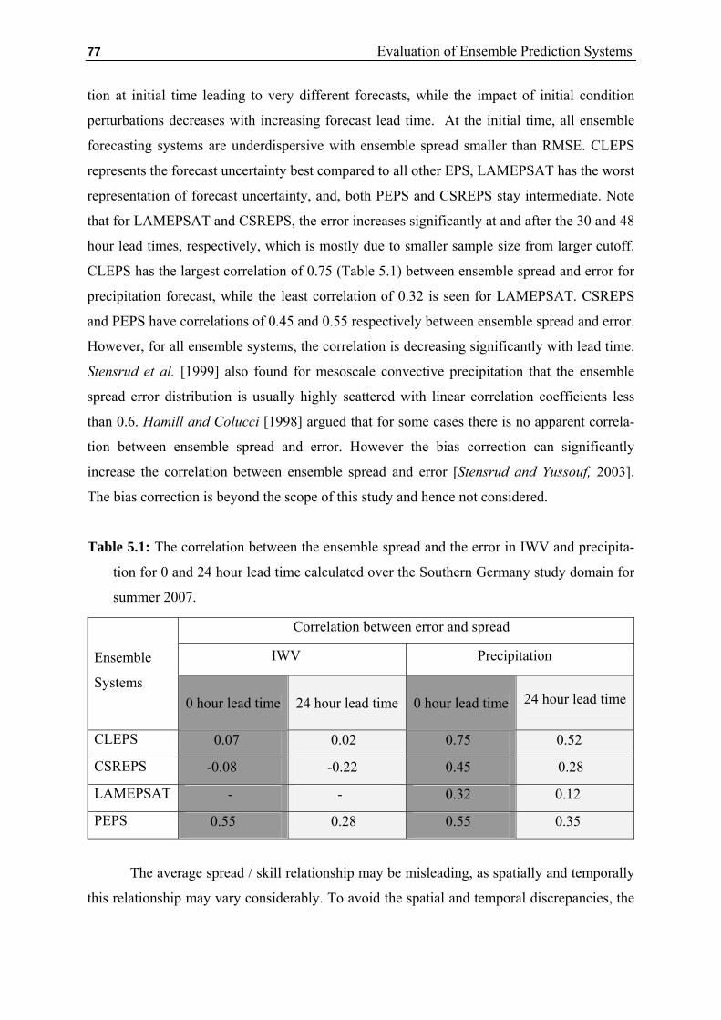
77 Evaluation of Ensemble Prediction Systems
tion at initial time leading to very different forecasts, while the impact of initial condition
perturbations decreases with increasing forecast lead time. At the initial time, all ensemble
forecasting systems are underdispersive with ensemble spread smaller than RMSE. CLEPS
represents the forecast uncertainty best compared to all other EPS, LAMEPSAT has the worst
representation of forecast uncertainty, and, both PEPS and CSREPS stay intermediate. Note
that for LAMEPSAT and CSREPS, the error increases significantly at and after the 30 and 48
hour lead times, respectively, which is mostly due to smaller sample size from larger cutoff.
CLEPS has the largest correlation of 0.75 (Table 5.1) between ensemble spread and error for
precipitation forecast, while the least correlation of 0.32 is seen for LAMEPSAT. CSREPS
and PEPS have correlations of 0.45 and 0.55 respectively between ensemble spread and error.
However, for all ensemble systems, the correlation is decreasing significantly with lead time.
Stensrud et al. [1999] also found for mesoscale convective precipitation that the ensemble
spread error distribution is usually highly scattered with linear correlation coefficients less
than 0.6. Hamill and Colucci [1998] argued that for some cases there is no apparent correla-
tion between ensemble spread and error. However the bias correction can significantly
increase the correlation between ensemble spread and error [Stensrud and Yussouf, 2003].
The bias correction is beyond the scope of this study and hence not considered.
Table 5.1: The correlation between the ensemble spread and the error in IWV and precipita-
tion for 0 and 24 hour lead time calculated over the Southern Germany study domain for
summer 2007.
The average spread / skill relationship may be misleading, as spatially and temporally
this relationship may vary considerably. To avoid the spatial and temporal discrepancies, the
Ensemble
Systems
Correlation between error and spread
IWV Precipitation
0 hour lead time 24 hour lead time 0 hour lead time 24 hour lead time
CLEPS 0.07 0.02 0.75 0.52
CSREPS -0.08 -0.22 0.45 0.28
LAMEPSAT - - 0.32 0.12
PEPS 0.55 0.28 0.55 0.35
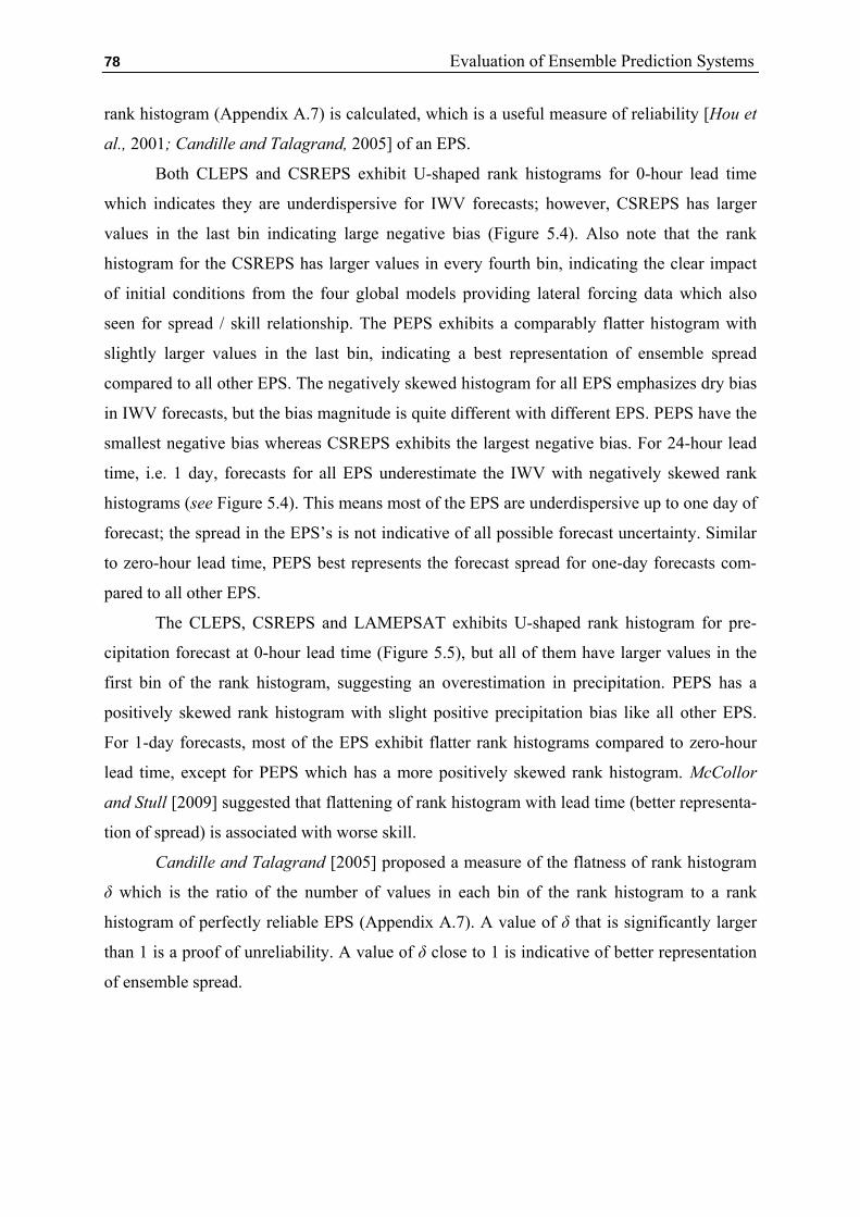
78 Evaluation of Ensemble Prediction Systems
rank histogram (Appendix A.7) is calculated, which is a useful measure of reliability [Hou et
al., 2001; Candille and Talagrand, 2005] of an EPS.
Both CLEPS and CSREPS exhibit U-shaped rank histograms for 0-hour lead time
which indicates they are underdispersive for IWV forecasts; however, CSREPS has larger
values in the last bin indicating large negative bias (Figure 5.4). Also note that the rank
histogram for the CSREPS has larger values in every fourth bin, indicating the clear impact
of initial conditions from the four global models providing lateral forcing data which also
seen for spread / skill relationship. The PEPS exhibits a comparably flatter histogram with
slightly larger values in the last bin, indicating a best representation of ensemble spread
compared to all other EPS. The negatively skewed histogram for all EPS emphasizes dry bias
in IWV forecasts, but the bias magnitude is quite different with different EPS. PEPS have the
smallest negative bias whereas CSREPS exhibits the largest negative bias. For 24-hour lead
time, i.e. 1 day, forecasts for all EPS underestimate the IWV with negatively skewed rank
histograms (see Figure 5.4). This means most of the EPS are underdispersive up to one day of
forecast; the spread in the EPS’s is not indicative of all possible forecast uncertainty. Similar
to zero-hour lead time, PEPS best represents the forecast spread for one-day forecasts com-
pared to all other EPS.
The CLEPS, CSREPS and LAMEPSAT exhibits U-shaped rank histogram for pre-
cipitation forecast at 0-hour lead time (Figure 5.5), but all of them have larger values in the
first bin of the rank histogram, suggesting an overestimation in precipitation. PEPS has a
positively skewed rank histogram with slight positive precipitation bias like all other EPS.
For 1-day forecasts, most of the EPS exhibit flatter rank histograms compared to zero-hour
lead time, except for PEPS which has a more positively skewed rank histogram. McCollor
and Stull [2009] suggested that flattening of rank histogram with lead time (better representa-
tion of spread) is associated with worse skill.
Candille and Talagrand [2005] proposed a measure of the flatness of rank histogram
δ which is the ratio of the number of values in each bin of the rank histogram to a rank
histogram of perfectly reliable EPS (Appendix A.7). A value of δ that is significantly larger
than 1 is a proof of unreliability. A value of δ close to 1 is indicative of better representation
of ensemble spread.

79 Evaluation of Ensemble Prediction Systems
Figure 5.4: Rank histogram in IWV for 0 hour lead time (left panel) and 24 hour lead time
(right panel) for (a, b) CLEPS, (c, d) CSREPS, (e, f) PEPS over the Southern Germany
study domain for summer 2007.
a) b)
c) d)
e) f)

80 Evaluation of Ensemble Prediction Systems
.
Figure 5.5: Rank histogram in precipitation for 0 hour lead time (left panel) and 24 hour lead
time (right panel) for (a, b) CLEPS, (c, d) CSREPS, (e, f) LAMEPSAT, (g, h) PEPS over
the Southern Germany study domain for summer 2007.
a) b)
c) d)
e) f)
g) h)
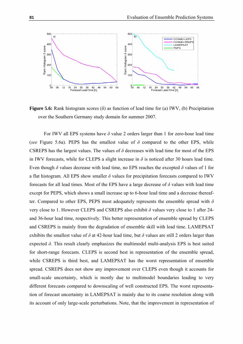
81 Evaluation of Ensemble Prediction Systems
Figure 5.6: Rank histogram scores (δ) as function of lead time for (a) IWV, (b) Precipitation
over the Southern Germany study domain for summer 2007.
For IWV all EPS systems have δ value 2 orders larger than 1 for zero-hour lead time
(see Figure 5.6a). PEPS has the smallest value of δ compared to the other EPS, while
CSREPS has the largest values. The values of δ decreases with lead time for most of the EPS
in IWV forecasts, while for CLEPS a slight increase in δ is noticed after 30 hours lead time.
Even though δ values decrease with lead time, no EPS reaches the excepted δ values of 1 for
a flat histogram. All EPS show smaller δ values for precipitation forecasts compared to IWV
forecasts for all lead times. Most of the EPS have a large decrease of δ values with lead time
except for PEPS, which shows a small increase up to 6-hour lead time and a decrease thereaf-
ter. Compared to other EPS, PEPS most adequately represents the ensemble spread with δ
very close to 1. However CLEPS and CSREPS also exhibit δ values very close to 1 after 24-
and 36-hour lead time, respectively. This better representation of ensemble spread by CLEPS
and CSREPS is mainly from the degradation of ensemble skill with lead time. LAMEPSAT
exhibits the smallest value of δ at 42-hour lead time, but δ values are still 2 orders larger than
expected δ. This result clearly emphasizes the multimodel multi-analysis EPS is best suited
for short-range forecasts. CLEPS is second best in representation of the ensemble spread,
while CSREPS is third best, and LAMEPSAT has the worst representation of ensemble
spread. CSREPS does not show any improvement over CLEPS even though it accounts for
small-scale uncertainty, which is mostly due to multimodel boundaries leading to very
different forecasts compared to downscaling of well constructed EPS. The worst representa-
tion of forecast uncertainty in LAMEPSAT is mainly due to its coarse resolution along with
its account of only large-scale perturbations. Note, that the improvement in representation of

82 Evaluation of Ensemble Prediction Systems
ensemble spread with increasing lead time by all EPS is due to the decrease of forecast skill
with forecast period as shown in previous section (Figure 5.3).
5.3 Assessment of Probabilistic Forecast Skill
Single verification measures are not sufficient to determine the performance of proba-
bilistic forecasts of the ensemble prediction systems [Murphy and Winkler, 1987; Murphy,
1991b] because of the multidimensionality of the forecast. In order to fully diagnose the
probability forecast, Murphy [1993] has shown that along with ensemble skill, reliability,
resolution, and sharpness attributes have to be verified, which emphasizes the different
aspects of forecast performance. Reliability indicates the extent to which a PDF estimate
proves close, a posteriori, to the distribution of observations, when this PDF estimate is
predicted. A prediction system which just predicts climatological frequency is a perfectly
reliable system. Resolution indicates the extent to which different forecast categories do in
fact reflect different frequencies of occurrence of the observed event. The deterministic
forecast has perfect resolution if it provides 0 or 1 probability value for a particular event
considered. Sharpness measures how much a forecast differs from the climatological mean
probability of the event. It only measures the variability of forecast and not the skill with
respect to observational truth. The performance of the ensemble prediction systems with
respect to these verification attributes for a complete probability density function (CPDF) and
for five thresholds for all key variables is explored in this section. The CPDF measures the
overall performance of the EPS for all possible events, while different thresholds are indica-
tive of the EPS performance for specific events. The quantile thresholds are chosen to define
the forecast events instead of actual values of the forecast, as forecast skill can be overstated
or understated when the samples are drawn from inhomogeneous datasets (e.g., different
season, regions with different probability of occurrence of event). Hamill and Juras [2006]
suggested the use of stratified samples, by season and for single stations or homogeneous
regions or alternatively, quantiles to define the forecast events instead of actual values of the
weather variable. The five thresholds are chosen on the basis of observational quantiles; 10%,
25%, 50%, 75%, and 90%, which are indicative of the very small, small, moderate, strong,
and very strong events. The events are defined at each station for IWV and on each grid cell
for precipitation with ensemble forecast exceeding the respective quantile thresholds. LCC
and HCC are categorical variables defined as values exceeding 50% threshold (Chapter 2
Section 2.5), thus it is considered as a representative of the 50% quantile threshold. Ensemble
83 Evaluation of Ensemble Prediction Systems
forecasts are converted to probabilistic forecasts by determining what percentage of the
ensemble members meets the specific event criterion.
5.3.1 EPS Forecast Skill for Specific Events
The EPS skills in the prediction of all key variables for five events are assessed by the
Brier skill score and its resolution and reliability component. The Brier score is defined as the
mean-square error of the probabilistic forecast, and it is one of the most widely used EPS
evaluation scores [Brier, 1950; Appendix A.8]. The Brier skill score is calculated as the Brier
score against a reference forecast. The reference forecast for the Brier skill score is the
climatological forecast in which the probability of the event is derived from the average of all
observations in the sample. The Brier skill score (BSS) can be decomposed into relative
reliability and relative resolution, which measure the reliability and resolution attributes of
EPS, respectively. BSS is a positive-oriented score, with BSS of 1 for perfect forecast, while
perfect forecasts would have the relative reliability equal to 0 and relative resolution equal to
1.
The ensemble prediction systems evaluated in this study have different ensemble siz-
es, CLEPS, CSREPS and LAMEPSAT have 16 ensemble members, while PEPS consist of
only 9 members. Thus to have a fair comparison, the Richardson [2001] transformation of the
Brier score and its component from M ensemble members to the Brier score for ∞ ensemble
members is used (Appendix A.8).
The temporal evolution of the Brier skill score and its two components, relative relia-
bility and relative resolution in IWV, for all five quantile thresholds are depicted in Figure
5.7. Most of the EPS have a constant decrease of BSS with forecast lead time, which clearly
indicates the degradation of forecast skill with forecast length. PEPS has the best BSS for all
five thresholds compared to all other EPS. CLEPS and CSREPS have almost similar skill for
most of thresholds except for the 10% and 25% quantile thresholds. All EPS show the best
skill for the 75% quantile threshold and the worst skill for the 10% quantile. PEPS has the
largest BSS of 0.62 for the 75% quantile and the least BSS of 0.2 for the 10% quantile.
CSREPS exhibits negative BSS for the 10% quantile whereas CLEPS has a very small
positive skill for zero-hour lead time, and negative BSS thereafter. For most of the thresholds,
CLEPS has better skill than CSREPS except for the 90% quantile threshold, where CSREPS
has a slightly better skill up to 18 hours lead time. Decrease of CSREPS skill after 18 hours
lead time may be because of smaller sample size for larger cutoff hours. Better skill of
CSREPS for the 90% quantile compared to CLEPS highlights the improvement of EPS skill

84 Evaluation of Ensemble Prediction Systems
for stronger events by the inclusion of small scale perturbations. The worst skill for the 10%
quantile threshold is due to the poor reliability and also poor resolution for all EPS (Figure
5.7a). However, for all other events, all EPS exhibit adequate resolution and reliability.
To better understand poor representation of EPS reliability for the 10% quantile
threshold (very small event), reliability diagrams for 10% and 70% quantile thresholds are
assessed. A reliability diagram is a diagram between the observed relative frequency and the
forecast probability for the particular thresholds corresponding to the forecast event [Wilks,
1995; Toth et al., 2003]. For the ideal probabilistic forecast, observation points lie on the
diagonal of the reliability diagram, indicating the event is always forecasted at the same
frequency as observed (see Appendix A.10). Also, the sharpness diagram is plotted along
with the reliability diagram which characterizes the relative frequency of occurrence of the
forecast probability category. The sharper EPS will have a forecast probability frequently
near 0 or 1, which indicates the forecasts deviate significantly from the climatological mean.
Reliability curves of IWV for the 10% quantile lie above the diagonal for most of the
forecast probabilities, except for the largest forecast probabilities, where all EPS are very
close to the diagonal (Figure 5.8a). Hence all EPS underestimate the occurrence of very small
IWV events when they predict rather smaller probabilities. Large underestimation for small
forecast probabilities is seen for all EPS whereas large probabilities are comparably well
forecasted by all EPS. The shallow slope of reliability curves for all EPS indicates the condi-
tional bias in IWV and reflects the fact that all EPS are overconfident. All EPS have a very
high degree of sharpness, indicating forecasts are not clustered near the climatological mean.
This implies no EPS is able to predict the very small forecast probabilities. All EPS exhibit
very good reliability for the 75% quantile threshold for IWV forecasts with slight underesti-
mation (Figure 5.8b). The reliability curve for the 75% quantile threshold also shows an
overall correct slope indicating no EPS is overconfident. All EPS show a high degree of
sharpness for the 75% quantile threshold; however, small probabilities are overestimated
compared to large probabilities. This clearly implies that all EPS underestimate the smaller
events while overestimating the larger events.
To better understand the poor EPS resolution for the 10% quantile threshold, EPS res-
olution is further investigated by using a Relative Operating Characteristic (ROC) curve and
skill score for area under the ROC curve (ROCSS). The ROC is a graph of the hit rate (HR)
against false alarm rate (FAR) for specific decision thresholds (Appendix A.11).

85 Evaluation of Ensemble Prediction Systems
Figure 5.7: Brier skill score (solid lines), relative reliability (line plus symbols), and relative
resolution (dashed lines) in IWV as function of lead time over the Southern Germany
study domain for summer 2007. (a) 10% quantile, (b) 25% quantile, (c) 50% quantile, (d)
75% quantile, and (e) 90% quantile thresholds.
All EPS exhibits large FAR for the 10% quantile threshold, but they have also large
HR (Figure 5.9a). PEPS has a higher HR compared to all other EPS and thus also the largest
ROCSS of 0.92. CLEPS and CSREPS have almost similar HR and also similar ROCSS of
0.75 and 0.73 respectively. Note that ROCSS for all EPS is higher than the generally accept-
a)
c) d)
e)
b)

86 Evaluation of Ensemble Prediction Systems
ed lower limit of useful resolution, 0.7. For the 75% quantile threshold, PEPS has a similar
discrimination as in the 10% quantile with very small FAR. CLEPS and CSREPS also have
very small FAR for the 75% quantile with ROCSS of 0.86 and 0.81 respectively (Figure
5.9b). As ROCSS for the 10% and 75% quantile thresholds are almost similar to each other,
the difference in BSS for them is mainly dominated by relative reliability.
Figure 5.8: IWV reliability diagram for CLEPS, CSREPS, and PEPS over the Southern
Germany study domain for summer 2007 (a) 10% quantile (b) 75% quantile thresholds.
Figure 5.9: IWV ROC curve for CLEPS, CSREPS, and PEPS over the Southern Germany
study domain for summer 2007 (a) 10% quantile (b) 75% quantile thresholds.
a) b)
a) b)

87 Evaluation of Ensemble Prediction Systems
Figure 5.10: Brier skill score and its component (relative resolution and relative reliability)
depending on lead time over the Southern Germany study domain for summer 2007. (a)
for LCC, (b) for HCC.
Figure 5.11: LCC (a) Reliability diagram (b) ROC curves for CLEPS, CSREPS, and PEPS
over the Southern Germany study domain for summer 2007.
a) b)
a) b)
88 Evaluation of Ensemble Prediction Systems
Most of the EPS exhibit negative BSS for LCC forecasts, except for PEPS which has
a smaller positive BSS (Figure 5.10a). All EPS have similar very low relative resolution.
PEPS has the best reliability and CLEPS is second best, whereas CSREPS has the worst
reliability. The negative BSS for CLEPS, CSREPS, and LAMEPSAT in LCC is mainly due
to the large overestimation of forecast probability by them (Figure 5.11a), especially for large
forecast probabilities. PEPS has the best representation of forecast probability with a slight
overestimation compared to all other EPS. ROC curves show all EPS have small HR and
FAR (Figure 5.11b). LAMEPSAT exhibits small HR values which never exceed 0.6, howev-
er it also has a very small FAR. Note that ROCSS never exceeds the acceptable limit of 0.7
for all EPS. However PEPS has the best ROCSS which is closer to the acceptable limit, while
LAMEPSAT has the worst ROCSS. For HCC, no EPS has a BSS larger than zero; all EPS
also exhibit poor relative resolution and reliability. The reliability curves are flatter for all
EPS with strong overestimation for all forecast probabilities (Figure not shown). ROC curves
in HCC for all EPS are quite similar to LCC, however, they have smaller ROCSS than for
LCC.
A constant decrease of BSS for precipitation forecasts is seen for most of the EPS,
which implies degradation of forecast skill with forecast length, except for CLEPS and
LAMEPSAT (Figure 5.12). A large increase of BSS after 30 hours lead time is observed for
LAMEPSAT, which is mostly due to the smaller sample size from the large cutoff hours. The
slight increase of skill after 24 hours lead time for CLEPS is mainly due to large scale
perturbations leading to more skillful forecasts for medium range. PEPS has a larger BSS
compared to other EPS for most of the thresholds, except for very small events, where
CLEPS has larger BSS. CLEPS has a negative BSS for 90% quantile threshold whereas
LAMEPSAT has negative BSS for almost all thresholds. Similar to IWV for precipitation,
CLEPS and CSREPS have similar skill for most of the thresholds except for the very strong
events, which clearly implies the benefit of small scale perturbations for prediction of strong-
er events. Most of the EPS have similar skill for very small, small, and moderate events, and
large degradation of skill for strong and very strong events. Surprisingly, LAMEPSAT has
better skill for strong and very strong events compared to other events. The weaker skill of
LAMEPSAT for all thresholds is mainly due to its poor relative reliability and resolution,
whereas all other EPS have quite good reliability for most of the thresholds, though all of
them have poor resolution.

89 Evaluation of Ensemble Prediction Systems
Figure 5.12: Brier skill score (solid lines), relative reliability (dashed lines), and relative
resolution (line plus symbols) in precipitation depending on lead time over the Southern
Germany study domain for summer 2007. (a) 10% quantile, (b) 25% quantile, (c) 50%
quantile, (d) 75% quantile, and (e) 90% quantile thresholds.
The reliability curve in precipitation for the 10% quantile lies very close to diagonal
for CLEPS and CSREPS, whereas PEPS has slight underestimation for all forecast probabili-
a)
d) c)
e)
b)

90 Evaluation of Ensemble Prediction Systems
ties (Figure 5.13a). LAMEPSAT has large overestimation for most of the forecast probabili-
ties except for very small forecast probabilities. The flatter reliability diagram for
LAMEPSAT emphasizes the conditional bias, whereas for all other EPS the slope of reliabil-
ity curves is near 45o. All EPS have a very high degree of sharpness, indicating forecasts are
not clustered near the climatological mean; however, they have very large relative frequency
for small forecast probabilities and very small relative frequency for large forecast probabili-
ties, except for LAMEPSAT. This implies, except for LAMEPSAT, that all EPS are overes-
timating small forecast probabilities and underestimating large forecast probabilities. For the
75% quantile threshold, most of the EPS exhibit large overestimation for all forecast proba-
bilities, except for PEPS which has a slight underestimation at smaller probabilities and a
slight overestimation at larger probabilities. Except for PEPS, all EPS have flat reliability
curves, implying that all of them are overconfident.
Figure 5.13: Precipitation reliability diagram for CLEPS, CSREPS, and PEPS over the
Southern Germany study domain for summer 2007 (a) 10% quantile (b) 75% quantile
thresholds.
The ROC curve for the 10% quantile threshold of precipitation exhibits large HR and
very small FAR for most of the EPS, except for the LAMEPSAT, which has a medium HR
and FAR (Figure 5.14a). Most of the EPS have small ROCSS which is smaller than the
acceptable limit of useful resolution (0.7), except for PEPS which has ROCSS of 0.73. All
EPS have larger HR and smaller FAR for the 75% quantile threshold (Figure 5.14b). Note
that ROCSS for all EPS is smaller than the acceptable limit, though CLEPS and PEPS have
ROCSS very close to 0.7. Better skill of LAMEPSAT for strong and very strong events
a) b)

91 Evaluation of Ensemble Prediction Systems
compared to other events is mainly because it has a very small FAR compared to other
events.
Figure 5.14: Precipitation ROC curve for CLEPS, CSREPS, and PEPS over the Southern
Germany study domain for summer 2007 (a) 10% quantile (b) 75% quantile thresholds.
5.3.2 Global Skill of EPS’
The global skill of all EPS’ is evaluated by continuous ranked probability scores
(CRPS, Appendix A.9). CRPS measures the distance between the predicted and the observed
cumulative density functions (CDFs) of scalar variables. The CRPS is a negatively oriented
score, reaching its minimum value of zero for a perfect deterministic system. A higher value
of the CRPS indicates a lower skill of the EPS. The global resolution and reliability attributes
of EPS are evaluated by CRPS Potential (CRPSpot) and CRPS Reliability (Reli) component of
CRPS, respectively. Like CRPS, its two components are also negatively oriented; that is, the
smaller those scores are, the better the EPS. As CRPS considers complete probability density
functions, thus it is not calculated for LCC and HCC.
CLEPS shows the best performance for IWV with the smallest CRPS value of 1.8
kg/m2, while PEPS shows the worst performance with CRPS of 5.8 kg/m2, and CSREPS has
an intermediate performance (Figure 5.15a). A constant increase of CRPS is seen for CLEPS
and CSREPS with increasing forecast time, which is representative of the decrease of the
forecast performance with the lead time. For the PEPS, the CRPS shows a slight decrease
with lead time. The CRPSpot value indicates PEPS has the highest resolution compared to
CLEPS and CSREPS, with a magnitude of 1.2 kg/m2, while CLEPS and CSREPS have
similar resolutions with a CRPSpot value ~1.5 kg/m2. CLEPS and CSREPS exhibit very good
reliability with Reli values smaller than 1.2 kg/m2, whereas PEPS has the worst reliability
b) a)

92 Evaluation of Ensemble Prediction Systems
with a very large Reli value of 4.5 kg/m2. Worst global skill of PEPS for IWV forecast is
mostly contributed from the lack of reliability.
PEPS has the best global skill for precipitation forecasts with a very small CRPS val-
ue of 0.3 mm/3h, whereas LAMEPSAT shows the worst skill with a CRPS value of 0.45
mm/3h (Figure 5.15b). The PEPS and LAMEPSAT show a decrease of EPS skill with
forecast time. CLEPS and CSREPS show an increase of forecast performance up to one day
of forecast and decrease thereafter, which implies both the EPS have better global skill for
medium-range forecasts, even though CLEPS is developed for short-range forecasts.
CSREPS has a slightly larger skill than CLEPS, emphasizing the benefit of inclusion of
small-scale perturbations. All EPS have similar resolution, except for LAMEPSAT. A sharp
decrease of forecast resolution is seen for LAMEPSAT after 24 hours leads time, which is
mostly due to the smaller sample size. Most of the EPS have very good forecast reliability
with values very close to zero, except for LAMEPSAT, which has poor reliability. Thus the
worst global skill of LAMEPSAT for precipitation is mainly dominated by poor reliability
along with poor resolution. This mostly comes from the coarse model resolution along with
considering only large-scale perturbations.
Figure 5.15: CRPS score and its component as function of lead time over the Southern
Germany study domain for summer 2007 (a) IWV (b) precipitation.
5.4 Summary
Most EPS satisfy the equally likely conditions for both IWV and precipitation, except
for the PEPS in precipitation. The deviation of PEPS from the equally likely conditions is
mostly due the inclusion of models with convection parameterization as well as the convec-
tion-permitting models.
b) a)
93 Evaluation of Ensemble Prediction Systems
Both spread skill analysis and rank histogram show that PEPS best represents the
forecast uncertainty for IWV with slight underdispersion. For precipitation, spread skill
analysis shows CLEPS has a better representation of forecast uncertainty than PEPS, whereas
the rank histogram shows PEPS has the best spread. As spread skill analysis is based on the
average skill over all stations/grid cells and period, it may be misleading. Thus we consider
PEPS to best represent the spread for precipitation. CLEPS better represents the forecast
uncertainty compared to CSREPS for both IWV and precipitation, whereas LAMEPSAT has
the worst representation of forecast uncertainty, which may be due to the coarse horizontal
resolution of model, and that it considers only large-scale uncertainty due to initial condi-
tions. All EPS have significant underdispersion in both IWV and precipitation except the
PEPS which has very small underdispersion.
Verification of EPS performance for different events shows PEPS has the best fore-
cast skill compared to other EPS in all key variables for most of the thresholds, whereas
LAMEPSAT shows the worst skill. This clearly implies that the benefits of multimodel
multiboundary perturbations are more beneficial for short-range prediction, while the worst
skill of LAMEPSAT is mainly due to its coarse resolution and only accounting large scale
perturbations into account. All EPS show poor skill for very small events (10% quantile) in
IWV, for all other events they show similar skill; this is due to the large underestimation of
small forecast probabilities, and all EPS are overconfident. For LCC and HCC forecasts, all
EPS have poor skill mainly because all produce large overestimates of forecast probabilities.
For precipitation, all EPS’ show a degradation of forecast skill with an increase of threshold,
where LAMEPSAT has negative skill for all thresholds. Degradation of skill with increasing
thresholds for precipitation forecasts by most of the EPS is mainly because of degradation of
reliability and resolution with large overestimation of forecast probabilities. For IWV and
precipitation forecasts, CLEPS shows better skill for very small, small and moderate events
compared to CSREPS, whereas CSREPS shows better skill for very strong events. This
clearly implies small-scale perturbations lead to an accurate forecast for stronger events for
the short range.
CLEPS shows good global skill and reliability in IWV which is similar to CSREPS.
PEPS shows very low global skill which is mostly dominated by the very low reliability, as
PEPS shows a good global resolution. For precipitation PEPS shows good global skill,
reliability, and resolution whereas LAMEPSAT shows the worst. CSREPS has slightly larger
global skill compared to CLEPS which is contributed by the better resolution.

94 Evaluation of Ensemble Prediction Systems
Marsigli et al. [2005] shows that CLEPS is not suitable for short-range forecasts be-
cause the main perturbations are designed to grow in the medium range and the sources of
small-scale error are not well described. CSREPS accounted small-scale perturbations
through the initial and boundary conditions from the mesoscale models as well as model
physics perturbation (Chapter 2). However, our analysis indicates that for precipitation
CSREPS is not beneficial over CLEPS for thresholds smaller than the 50% quantile. Never-
theless CSREPS have larger skill for the 75% and 90% quantiles, suggesting an improvement
for stronger events. Also for precipitation forecast CSREPS has a better global skill over
CLEPS. For IWV, CLEPS shows better global skill as well as better skill for different
thresholds compared to the CSREPS. The PEPS was more successful than all single model
EPS as it samples uncertainties in both the initial conditions and model formulation.

95
Chapter 6
Conclusions and Outlook
6.1 Summary and Conclusions
Precipitation is the end product of a complex process chain of the atmospheric water
cycle; thus errors in any component of the chain lead to inaccurate quantitative precipitation
forecasts (QPF). Most of the atmospheric water cycle processes are parameterized in models,
as they occur on scales smaller than models’ grid cells. Due to the limited understanding and
complexity in representing these atmospheric water cycle processes, a number of parameteri-
zation schemes are available with different assumptions. Limited accuracy of initial condi-
tions, due to sparse observational networks along with observational errors, also contributes
to errors in precipitation forecasts. Thus, the complete atmospheric water cycle forecast by
deterministic models and ensemble systems is evaluated in this dissertation to diagnose the
shortcomings in quantitative precipitation forecasts. Four key variables of the atmospheric
water cycle are evaluated: integrated water vapour (IWV), low cloud cover (LCC), high
cloud cover (HCC) and precipitation, which are representative of water in all three phases.
This comprehensive verification of the atmospheric water cycle is performed for nine deter-
ministic models and four ensemble systems from the forecast demonstration experiment
Mesoscale Alpine Programme (MAP D-PHASE) using measurements from the General
Observation Period (GOP) over Southern Germany for summer 2007. Verification of multi-
ple models and ensemble systems revealed specific models' weaknesses along with the causes
of shortcomings in QPF. We addressed these issues in detail in Chapters 3 through 5, and the
key findings are summarized in following sections.
How accurate can atmospheric water cycle variables be forecast by today’s mesoscale
models?
Verification of deterministic models is performed for three different aspects of model
forecasts such as amount, timing (temporal distribution), and regional distribution of all key
variables. Observed mean IWV is accurately forecasted by all COSMO models, while the
MM5 model shows ~5% overestimation and French models AROME and ALADFR show
~6% underestimation. Large IWV biases in MM5 and French models are likely due to
deficits in their driving models, ARPEGE and GFS, respectively. Observed shape of the
mean IWV diurnal cycle is very well reproduced by all models except for the above men-

96 Conclusions and Outlook
tioned offsets. However all model forecasts observed diurnal maxima a few hours (~0-3
hours) earlier than observations.
All COSMO models overestimate mean LCC frequency by ~45%, while the French
models AROME and ALADFR underestimate it by ~23% and the MM5 model overestimate
it by more than 100%. The over- and underestimation of LCC in MM5 and French models is
likely due to their respective large over- and underestimation of IWV. Although most of the
models forecast LCC maxima ~2 – 4 hours later than observations, the shape of the mean
LCC diurnal cycle is very well reproduced by all except the MM5 model. Most of the models
overestimate the mean HCC frequency by more than 100% compared to MSG observations.
This is likely due to underestimation in HCC frequency of MSG observations, as satellites
often miss optically thin high-level clouds. Very weak diurnal variability is observed in HCC;
all models forecast similar weak diurnal variability.
All models overestimate the mean precipitation rate by ~8–27%. Moreover, no model
is able to capture the observed mean diurnal variability. LOWRES models predict the maxi-
mum of the diurnal precipitation cycle ~2 – 8 hours earlier whereas HIGHRES models
predict diurnal precipitation maximum ~2 hours later. The sole exception is the AROME
model which shows large precipitation maxima 2 hours earlier than observations. The very
large diurnal precipitation maximum in the AROME model is mostly due to overestimation
in numerical diffusion, which induces too strong outflows under convective cells [Bauer et
al., 2011]. The COSMO models with parameterized convection show windward/lee effects in
regional distribution. As per Schwitalla et al. [2008], the possible reasons for this effect are
(i) inaccurate simulation of the flow at coarse resolution, and/or (ii) the convection parame-
terizations cannot account for cell motion and hydrometeor advection. In reality this effect
leads to a substantial separation between the location where convection is triggered and the
area where the rain reaches the ground. However, the windward/lee effect is not seen for
other models with parameterized convection.
Pronounced decreases in all key variables are observed at 1200 UTC for models
which are restarted at 1200 UTC. This is clearly due to the assimilation of daytime radio-
soundings. Daytime radiosoundings report too dry IWV values due to solar heating of meas-
urement sensors. Thus assimilation of these radiosounding observations into models intro-
duces a pronounced IWV dry bias on the order of ~6%. Clear error propagation in the process
chain from IWV to precipitation is seen in terms of a pronounced decrease at 1200 UTC for
all key variables.

97 Conclusions and Outlook
The observed regional distribution of key variables is not very well represented by
any models. All models exhibit large biases in all key variables over higher elevation regions.
Also all models show larger random error over regions of complex topography, which clearly
emphasizes the models' limitation in the prediction of these key variables over complex
topography. These results also suggest that even high resolution models do not resolve all
topographic structures. For all key variables, random errors are significantly larger than the
systematic error, specifically for HCC and precipitation.
Is the performance of convection-permitting high resolution models superior?
Most of the HIGHRES models overestimate IWV compared to their LOWRES coun-
terparts. LOWRES models show large error growth of ~24% per day compared to their
HIGHRES counterparts which have error growth of ~19% per day. However HIGHRES and
LOWRES models do not show any difference in forecast skill and also for representation of
the mean IWV diurnal cycle.
The mean LCC frequency and its regional distribution are better represented by all
HIGHRES models compared to their LOWRES counterparts. In addition, for LCC forecasts,
all HIGHRES models have smaller random error compared to their corresponding LOWRES
models. However, no clear difference between HIGHRES and LOWRES models is seen for
representation of diurnal variability in LCC. Also, for HCC forecasts, we do not see any clear
difference between HIGHRES and LOWRES models for amount, timing, and regional
distribution. Dependency of model resolution is not seen on error growth with forecast times
for the prediction of LCC and HCC. Domain mean and regional distribution of precipitation
are better represented by most of the HIGHRES models compared to their LOWRES coun-
terparts, except by the AROME model. HIGHRES models better represent mean diurnal
precipitation cycle compared to their LOWRES counterparts with a difference of only 2
hours to the observed precipitation maximum. LOWRES models predict precipitation maxi-
ma 2 – 8 hours earlier than observations. Compared to observations, COSMO LOWRES
models predict diurnal precipitation maxima ~6-8 hours earlier, while the MM5 model
predicts 2 hours earlier, which is mostly due to their different convection initiation criteria.
COSMO models use Tiedke convection scheme (T89), in which convection is initiated when
a parcel’s temperature exceeds the environment temperature by a fixed temperature threshold
of 0.5 K; whereas the MM5 model uses Grell’s convection scheme (G94), in which the
convection initiation criteria are based on the net column destabilization rate. It is most likely
that the net column destabilization rate-based convection initiation criteria in the G94 scheme
98 Conclusions and Outlook
better predict the time of convection initiation. However, Chaboureau et al. [2004] argued
that representation of succession of regimes, from dry to moist, non-precipitating to precipi-
tating, convection also plays a significant role in convection initiation. For precipitation
forecasts, most of the HIGHRES models show large error growth of ~35% per day corre-
sponding to their LOWRES models which have error growth of ~10% per day.
What is the most important factor, e.g. boundary conditions, model formulation or
resolution, affecting the forecast performance? Are there clusters of models for specific
factors such as model code, resolution, and driving model?
For prediction of IWV, LCC and HCC, model formulation is the most dominant fac-
tor. Models with the same formulation show similar systematic errors and also diurnal
variability. For precipitation forecasts, model resolution is the most dominant factor, because
summer precipitation is governed by convective rain which is treated differently in
HIGHRES and LOWRES models. Initial conditions are the second most dominant factor
affecting the forecast performance. Models with initial conditions from different global
models show clear discrepancies in forecasting regional distributions of HCC and precipita-
tion.
The positive impact of 3D-Var data assimilation over nudging is seen for precipitation
forecasts by the COSMO-IT model, which is not seen for the other three key variables.
Moreover, the positive impact of the 3D-Var data assimilation for AROME and ALADFR
models is seen for none of the key variables, which again clearly emphasizes model formula-
tion is a dominant factor affecting forecast performance.
For IWV forecast, models are clustered according to their code, and also models nest-
ed in each other are clustered together. However, for LCC forecasts, models are clustered
according to their code, but the clustering of models nested in each other is not seen. For
HCC forecasts, models cluster according to their formulation, and also cluster according to
their initial conditions. For precipitation forecasts, models are clustered according to their
resolution as HIGHRES and LOWRES models treat convection differently. Model formula-
tion is a second dominant factor for models to cluster together for precipitation forecasts.
Are observed similarities between the different key variables well represented by
models?
The similarities between the different key variables are assessed by means of linear
relationships by comparing the observed relationship with that from models. A weak linear

99 Conclusions and Outlook
relationship is observed between IWV and LCC with a rank correlation of 0.19. All COSMO
models underestimate this relationship with a rank correlation of ~0.15, while French models
overestimate this relationship with a rank correlation of 0.25. The MM5 model better repre-
sents the observed strength of the relationship between IWV and LCC, with a rank correla-
tion of 0.18. Moderate linear relationship strength is observed between IWV and HCC with a
rank correlation of 0.4, which is quite well represented by all models, but HIGHRES models
slightly underestimate (rank correlation ~0.36) and LOWRES models slightly overestimate
(rank correlation ~0.45). Moderate relationship strength is observed between IWV and
precipitation with a rank correlation of 0.33, which is very well reproduced by all models,
with slight underestimation in HIGHRES models (rank correlation ~0.29) and slight overes-
timation in LOWRES models (~0.35) except by MM5, which has a rank correlation of 0.48.
Stronger relationship strength is observed between LCC and precipitation with a rank correla-
tion of 0.43. All models strongly overestimate this relationship with a rank correlation of
0.55-0.68. This clearly indicates that the relationship between low cloud cover and precipita-
tion is misrepresented in models. However, most of the HIGHRES models slightly overesti-
mate the relationship strength between LCC and precipitation compared to their correspond-
ing LOWRES models, except AROME. A strong linear relationship is observed between
HCC and precipitation with a rank correlation of 0.54, which is clearly underestimated by all
models with a rank correlation of 0.35-0.45. However, HIGHRES models have stronger
underestimation compared to their corresponding LOWRES counterparts.
The atmospheric water cycle processes occurs with a certain time delay. Thus, key
variables can have larger linear relationships at a specific time lag. Observed time lags of
largest relationship between different key variables are compared with that from models to
determine how well models reproduce this time lag. A time lag of -9 hours is observed
between IWV and LCC, as the formation of LCC leads precipitation only after certain time
lags, which then leads to increases in IWV. This time lag between IWV and LCC is quite
well represented by most of the models except the French models, which show very small
time lag of ~5 hours. Very small time lag between IWV and LCC in the French models is due
to the misrepresentation of relationships between these two key variables. Observed IWV
does not show any time lag with HCC, as formation of precipitation leads to high clouds and
also increases IWV simultaneously. This observed time lag between IWV and HCC is very
well represented by all models. Observed time lag of -2 hour between IWV and precipitation
is also very well represented by all models. However, an observed time lag of 6 hours be-
tween LCC and precipitation is not represented by any of the models. COSMO HIGHRES
100 Conclusions and Outlook
and MM5 models show a time lag of only 2 hours, while COSMO LOWRES and French
models shows a time lag of 0 hours.
Do the ensemble prediction systems reflect the uncertainty in forecasting the key varia-
bles of the atmospheric water cycle?
Uncertainties in IWV and precipitation forecasts are very well represented by PEPS,
with slight underdispersion. CLEPS represents forecast uncertainty in IWV and precipitation
considerably better than CSREPS. LAMEPSAT has comparably poor representation of
forecast uncertainty for IWV and precipitation. The best representation of forecast uncertain-
ty by PEPS is likely due to the fact that it accounts for uncertainty by the initial conditions
and the model physics. Poor representation of forecast uncertainty by LAMEPSAT is mostly
due to its coarse horizontal resolution, and it accounts only the large-scale uncertainty by
initial conditions. CLEPS shows better ensemble spread compared to CSREPS, even though
CSREPS accounts for small-scale uncertainty due to initial and boundary conditions from the
limited-area model.
Which is the primary perturbation affecting the EPS performance at short range, the
initial conditions or the model physics? How reliable is a multi-model EPS?
PEPS shows the best forecast skill compared to other EPS in all key variables for
most of the events, whereas LAMEPSAT shows the worst skill. The better performance of
PEPS is mostly due to sample uncertainties in both the initial conditions and the model
formulation. The poor skill of LAMEPSAT is likely due to its coarse resolution and that it
accounts for only large-scale uncertainty by initial conditions.
All EPS show very poor skill for LCC and HCC forecasts, as a result of large overes-
timates of forecast probabilities. For precipitation, most of the EPS show a degradation of
forecast skill with an increase of threshold, which is mainly due to degradation of reliability
and resolution. CSREPS shows better skill over CLEPS for prediction of stronger events in
IWV and precipitation. This implies that small-scale perturbations due to the uncertainty in
initial and boundary conditions from limited-area models likely lead to an accurate forecast
for stronger events.
CLEPS shows better global skill in IWV, and is similar to CSREPS. PEPS has a very
low global skill for IWV forecasts perhaps due to its very low reliability. For precipitation
forecasts, PEPS has the best global skill, whereas LAMEPSAT shows the worst skill.

101 Conclusions and Outlook
CSREPS has slightly better global skill in precipitation forecasts compared to CLEPS as a
result of better resolution.
6.2 Scope of Future Research
Verification of the complete atmospheric water cycle from IWV and cloud cover to
precipitation at the ground reveals several model weaknesses. Nevertheless, this study is
restricted specifically due to limited availability of model forecasts. A comprehensive
evaluation of the complete atmospheric water cycle can be further elaborated by considering
the following aspects. Precipitation intensity is strongly controlled by cloud microphysics;
thus, the detailed validation of cloud microphysics will be advantageous to pinpoint the
shortcomings in QPF. Quantifying errors in representing specific atmospheric water cycle
processes can be done by changing their respective physical parameterization. However, such
studies are limited due to their high computation cost [Gallus and Pfeifer, 2008, five
microphysics scheme in WRF model]. The verification over different weather classifications
and over certain regions might be helpful to identify specific model deficiencies. However,
such studies require large forecast samples, as the smaller sample size can easily mislead
verification results. Long-term evaluation also might be more useful to point out the model
shortcomings, as it might average out stochastic errors arising due to the initial and boundary
conditions. Verification of EPS reveals that PEPS is the most skillful for short-range
prediction. Ensemble members of PEPS can be extended by adding more deterministic
models from operational centers. It is interesting to compare the skill of PEPS developed
from convection-parameterized models against convection-resolving models.

102 Conclusions and Outlook

103
References
Ament, F., T. Weusthoff, and M. Arpagaus, 2011: Evaluation of MAP D-PHASE heavy precipi-
tation alerts in Switzerland during summer 2007, Atmos. Res. 100, 2-3, 178-189.
Anderson, J. L., 1996: A method for producing and evaluating probabilistic forecasts from
ensemble model integrations. J. Climate, 9, 1518-1530.
Arakawa, A., and W. Schubert, 1974: Interaction of a cumulus ensemble with the large-scale
environment. Part I. J. Atmos. Sci., 31, 674-701.
Arakawa, A., 1972: Design of the UCL: A general circulation model. Tech. Rep. 7, 103 pp.
[Available from Dept. of Meteorology, c/o Mail Services, Box 951361, Los Angeles, CA
90095-1361.]
Arpagaus, M., M. W. Rotach, P. Ambrosetti, F. Ament, C. Appenzeller, H. S. Bauer, A. Beh-
rendt, F. Bouttier, A. Buzzi, M. Corazza, S. Davolio, M. Denhard, M. Dorninger, L. Fon-
tannaz, J. Frick, F. Fundel, U. Germann, T. Gorgas, G. Grossi, C. Hegg, A. Hering, S. Jaun,
C. Keil, M. A. Liniger, C. Marsigli, R. McTaggart-Cowan, A. Montani, K. Mylne, L. Pan-
ziera, R. Ranzi, E. Richard, A. Rossa, D. Santos-Muñoz, C. Schär, Y. Seity, M. Staudinger,
M. Stoll, S. Vogt, H. Volkert, A. Walser, Y. Wang, J. Werhahn, V. Wulfmeyer, C. Wunram,
and M. Zappa, 2009: MAP D-PHASE. Demonstrating forecast capabilities for flood events
in the Alpine region, Veröffentlichungen der MeteoSchweiz, 78, 75.
Austin, P. M., 1987: Relation between measured radar reflectivity and surface rainfall. Mon.
Weather Rev., 115, 1053-1070.
Back, L. E., and C. S. Bretherton, 2010: The relationship between wind speed and precipitation
in the Pacific ITCZ. J. Climate., 18, 4317-4328.
Barnett, T. P., J. Ritchie, J. Gloat, and G. Stokes, 1998: On the space-time scales of the surface
solar radiation field, J. Climate., 11, 88-96.
Barrett, A. I., R. J. Hogan, and E. J. O’Connor, 2009: Evaluating forecasts of the evolution of the
cloudy boundary layer using diurnal composites of radar and lidar observations. Geoph. Res.
Let., 36(17), 1-5. doi:10.1029/2009GL038919.

104
Bauer, H. S., T. Weusthoff, M. Dorninger, V. Wulfmeyer, T. Schwitalla, T. Gorgas, M. Arp-
agaus, and K. Warrach-Sagi, 2011: Predictive skill of a subset of models participating in D-
PHASE in the COPS region. Quar. J. Roy. Meteorol. Soc., 137(S1), 287-305.
doi:10.1002/qj.715.
Bechtold, P., E. Bazile, F. Guichard, P. Mascart and E. Richard, 2001: A mass-flux convection
scheme for regional and global models. Q. J. Roy. Meteor. Soc., 127, 869-886.
Bechtold, P., M. Köhler, T. Jung, F. Doblas-Reyes, M. Leutbecher, M. J. Rodwell, F. Vitart, and
G. Balsamo, 2008: Advances in simulating atmospheric variability with the ECMWF model:
From synoptic to decadal time-scales. Q. J. Roy. Meteor. Soc., 134, 1337–1351, doi:10.1002
/qj.289.
Bei, N., and F. Zhang, 2007: Impacts of initial condition errors on mesoscale predictability of
heavy precipitation along the Mei-Yu front of China. Q. J. Roy. Meteor. Soc, 133, 83-99.
Bellon, A., G. Lee, and I. Zawadzki, 2005: Error statistics of VPR corrections in stratiform
precipitation. J. Appl. Meteorol., 44, 998-1015.
Betts, A. K., and C. Jakob, 2002: Evaluation of the diurnal cycle of precipitation, surface ther-
modynamics and surface fluxes in the ECMWF model using LBA data. J. Geophy. Res.,
107, 8045, doi: 10.1029/2001JD000427
Betts, A., and M. Miller, 1986: A new convective adjustment scheme. Part II: Single column
tests using GATE wave, BOMEX, ATEX and arctic air-mass data sets. Q. J. Roy. Meteor.
Soc., 112, 693-709.
Böhme, T., S. Stapelberg, T. Akkermans, S. Crewell, J. Fischer, T. Reinhardt, A. Seifert, C.
Selbach, and N. Van Lipzig, 2011: Long-term evaluation of COSMO forecasting using
combined observational data of the GOP period. Meteorologische Zeitschrift, 20(2), 119-
132. doi:10.1127/0941-2948/2011/0225.
Bougeault, P., 1985: A simple parameterization of the large-scale effects of cumulus convection.
Mon. Weather Rev., 113, 2108-2121.
Bougeault, P., P. Binder, A. Buzzi, R. Dirks, J. Kuettner, R. Houze, R. B. Smith, R. Steinacker,
H. Volkert, 2001: The MAP special observing period. Bull. American Meteorol. Soc., 82(3),
433-462.
105
Bouteloup, Y., E. Bazile, F. Bouyssel and P. Marquet, 2009: Evolution of the physical parametri-
sations of ARPEGE and ALADIN-MF models. Aladin Newsletter Nr35 p48-58.
Bowler, N.E., A, Arribas, K.R. Mylne, K.B., Robertson, S.E. Beare, 2008: The MOGREPS
short-range ensemble prediction system. Q. J. Roy. Meteor. Soc., 134, 703-722.
Brier, G. W., 1950: Verification of forecasts expressed in terms of probabilities. Mon. Weather.
Rev., 78, 1-3.
Brusch, S., 2006: Fernerkundung des luftdrucks am oberrand von wolken mit MSG - SEVIRI.
Diploma thesis, Freie Universität Berlin, 111pp.
Buzzi, A., M. Fantini, P. Malguzzi and F. Nerozzi, 1994: Validation of a limited area model in
cases of mediterranean cyclogenesis: Surface fields and precipitation scores, Meteo. Atmos.
Phys., 53, 3-4, 137-153, DOI: 10.1007/BF01029609.
Candille, G., and O. Talagrand, 2005: Evaluation of probabilistic prediction systems for a scalar
variable. Q. J. Roy. Meteor. Soc., 131, 2131-2150.
Chaboureau, J.P., and P. Bechtold, 2005: Statistical representation of clouds in a regional model
and the impact on the diurnal cycle of convection during Tropical Convection, Cirrus and
Nitrogen Oxides (TROCCINOX). J. Geoph. Res., 110(D17), 1-11. doi 10.1029
/2004JD005645.
Chaboureau, J.P., P. Tulet, and C. Mari, 2007: Diurnal cycle of dust and cirrus over West Africa
as seen from Meteosat Second Generation satellite and a regional forecast model. Geophy.
Res. Let., 34(2), 1-5. doi:10.1029/2006GL027771.
Chaboureau, J.P., F. Guichard, J.-L. Redelsperger, and J.-P. Lafore, 2004: The role of stability
and moisture in the diurnal cycle of convection over land. Q. J. Roy. Meteor. Soc., 130,
3105-3117.
Chen, F., and J. Dudhia, 2001: Coupling an advanced land surface- hydrology model with the
Penn State–NCAR MM5 modeling system. Part I: Model implementation and sensitivity.
Mon. Wea. Rev., 129, 569-585.

106
Chen, F., K. Mitchell, J. Schaake, Y. Xue, H. Pan, V. Koren, Q. Duan, and A. Betts, 1996:
Modeling of land-surface evaporation by four schemes and comparison with FIFE observa-
tions. J. Geophys. Res., 101, 7251-7268.
Chen, J., J.S. Xue, and H. Yan, 2005: A new initial perturbation method of ensemble mesoscale
heavy rain prediction. Chinese J. Atmos. Sci. 5: 717-726.
Cherubini, T., A. Ghelli, and F. Lalaurette, 2002: Verification of precipitation forecasts over the
Alpine region using a high-density observing network. Weather. Forecast., 17, 238-249.
Clark, A. J., W. A. Gallus, and T. C. Chen, 2007: Comparison of the diurnal precipitation cycle
in convection-resolving and non-convection-resolving mesoscale models. Mon. Weather
Rev., 135, 3456-3473.
Clark, A. J., W. A. Gallus, M. Xue, and F. Kong, 2009: A comparison of precipitation forecast
skill between small convection allowing and large convection parameterizing ensembles.
Weather Forecast, 24, 1121-1140.
Comstock, J. M., and C. Jakob, 2004: Evaluation of tropical cirrus cloud properties derived from
ECMWF model output and ground based measurements over Nauru Island. Geophy. Res.
Let., 31(10), doi: 10.1029/2004GL019539.
Cook, B. I., G.B. Bonan, and S. Levis, 2006: Soil moisture feedbacks to precipitation in southern
Africa. J. Climate, 19, 4198-4206.
Crewell, S., M. Mech, T. Reinhardt, C. Selbach, H.D. Betz, E. Brocard, G. Dick, E. O'Connor, J.
Fischer, T. Hanisch, T. Hauf, A. Hünerbein, L. Delobbe, A. Mathes, G. Peters, H. Wernli,
M. Wiegner, and V. Wulfmeyer, 2008: The general observation period 2007 within the pri-
ority program on quantitative precipitation forecasting: Concept and first results. Meteorolo-
gische Zeitschrift, 17(6), 849-866. doi: 10.1127 /0941-2948/2008/0336.
Cuxart, J., Ph. Bougeault, and J. L. Redelsperger, 2000: A turbulence scheme allowing for
mesoscale and large-eddy simulations. Quar. J. Roy. Meteorol. Soc., 126, 1-30.
Davis, J. L., T. A. Herring, I. I. Shapiro, A. E. E. Rogers, and G. Elgered, 1985: Geodesy by
radio interferometry: Effects of atmospheric modeling errors on estimates of baseline length,
Radio Sci., 20, 1593-1607.

107
Deardorff, J. W., 1978: Efficient prediction of ground surface temperature and moisture with
inclusion of a layer of vegetation. J. Geophys. Res., 93, 1889-1903.
Delrieu, G., J.D. Creutin, and I. Saint-Andre, 1991: Mean K-R relationships: Practical results for
typical weather radar wavelengths. J. Atmos. Oceanic Technol., 8, 467-476.
Dessler, A.E., and P. Yang, 2003: The distribution of tropical thin cirrus clouds inferred from
Terra MODIS data. J. Climate., 16, 1241-1247.
Dick, G., G. Gendt, and C. Reigber, 2001: First experience with near real-time water vapor
estimation in a German GPS network, J. Atmos. Solar Terres. Phys., 63, 1295- 1304.
Doerflinger, E., R. Bayer, J. Chery, and B. Bürki, 1998: The Global Positioning System in
mountainous areas: Effect of the troposphere on the vertical accuracy, C.R. Acad. Sci. Paris,
326, 319- 325.
Doms, G., J. Forstner, E. Heise, H.-J. Herzog, M. Raschendorfer, T. Reinhardt, B. Ritter, R.
Schrodin, J.-P. Schulz, and G. Vogel, 2007: A description of the nonhydrostatic regional
model LM: Physical parameterization. Deutscher Wetterdienst, Offenbach, pp. 23-24
(www.cosmomodel.org/content/model/documentation/core/ cosmo Phys- Paramtr.pdf).
Du, J., S. L. Mullen, and F. Sanders, 1997: Short-range ensemble forecasting of quantitative
precipitation. Mon. Weather Rev. 125: 2427–2459.
Du, J., 2007: Uncertainty and ensemble forecast. Science and Technology. Retrieved from
http://www.weather.gov/ost/climate/STIP/STILecture1.pdf
Du, J., and M. S. Tracton, 2001: Implementation of a real-time short-range ensemble forecasting
system at NCEP: an update. Preprints, 9th Conference on Mesoscale Processes, Ft. Lauder-
dale, Florida, Amer. Meteor. Soc., 355-356.
Ebert, E. E., 2001: Ability of a poor man’s ensemble to predict the probability and distribution of
precipitation. Mon. Weather. Rev., 129, 2461-2480.
Ebert, E.E., U. Damrath, W. Wergen, and M.E. Baldwin, 2003: The WGNE assessment of short-
term quantiatitve precipitation forecasts. Bull. Amer. Meteor. Soc., 84, 481-492.
Efron, B., 1979: Bootstrap methods: Another look at the jack knife. Ann. Stat., 7, 1-26.
108
Fabry, F., and I. Zawadzki, 1995: Long-term radar observations of the melting layer of precipita-
tion and their interpretation. J. Atmos. Sci., 52, 838-851.
Findell, K. L., and E. A. B. Eltahir, 2003: Atmospheric controls on soil moisture- boundary layer
interactions. Part I: Framework development. J. Hydrometeor., 4, 552-569.
Frei, C., and C. Schär, 1998: A precipitation climatology of the Alps from high-resolution rain-
gauge observations. Inter. J. Climat., 18(8), 873-900.
Frei, C., J. H. Christensen, M. Déqué, D. Jacob, R. G. Jones, and P. L. Vidale, 2003: Daily
precipitation statistics in regional climate models: Evaluation and intercomparison for the
European Alps, J. Geophys. Res., 108(D3), 4124, doi:10.1029/2002JD002287.
Fritsch, J. M., and R. E. Carbone, 2004: Improving quantitative precipitation forecasts in the
warm season. Bull. Amer. Meteor. Soc., 85, 955-965.
Gallus, Jr, W. A., and M. Pfeifer, 2008: Intercomparison of simulations using 5 WRF microphys-
ical schemes with dual-Polarization data for a German squall line. Adv. Geosciences, 16,
109-116.
Ghelli, A., and F. Lalaurette, 2000: Verifying precipitation forecasts using upscaled observa-
tions. ECMWF Newsletter, Vol. 87, 9– 17.
Gilmore, M. S., J. M. Straka and E. N. Rasmussen, 2004: Precipitation uncertainty due to varia-
tions in precipitation particle parameters within a simple microphysics scheme. Mon.
Weather Rev., 132, 2610-2627.
Grabowski, W. W., 2003: MJO-like coherent structures: Sensitivity simulations using the cloud-
resolving convection parameterization (CRCP). J. Atmos. Sci., 60, 847-864.
Grell, G. A., J. Dudhia, and D. R. Stauffer, 1994: A description of the fifth generation Penn
State/NCAR Mesoscale Model (MM5), NCAR/TN- 398 STR, 122 pp., Natl. Cent. for Atmos.
Res., Boulder, Colorado.
Grimit, E. P., C. F. Mass, 2007: Measuring the ensemble spread–error relationship with a proba-
bilistic approach: Stochastic ensemble results. Mon. Weather. Rev., 135, 203-221.
Grimit, E.P., and C.F. Mass, 2002: Initial results of a mesoscale short-range ensemble forecast-
ing system over the pacific northwest. Weather Forecast, 17, 192-205.

109
Guerova, G., E. Brockmann, F. Schubiger, J. Morland, and C. Mätzler, 2005: An integrated
assessment of measured and modeled integrated water vapor in Switzerland for the period
2001-03. J. Appl. Meteor., 44, 1033-1044.
Guerova, G., E. Brockmann, J. Quiby, F. Schubiger, and C. Mätzler, 2003: Validation of NWP
mesoscale models with Swiss GPS network AGNES. J. Appl. Meteor., 42, 141-150.
Guichard, F., J. C. Petch, J.L. Redelsperger, P., Bechtold, J.P., Chaboureau, S., Cheinet, W.
Grabowski, H., Grenier, C. G. Jones, M. Köhler, J. M. Piriou, R. Tailleux, M. Tomasini,
2004: Modelling the diurnal cycle of deep precipitation convection over land with cloud re-
solving models and single column models. Q. J. Roy. Meteor. Soc., 130, 3139-3172.
Hamill, T. M., and J. Juras, 2006: Measuring forecast skill: is it real skill or is it the varying
climatology?, Quar. J. Roy. Meteorol. Soc., 132, 2905-2923.
Hamill, T. M., and S. J. Colucci, 1998: Evaluation of eta-RSM ensemble probabilistic precipita-
tion forecasts. Mon. Weather. Rev., 126, 711-724.
Hamill, T. M., 2001: Interpretation of rank histograms for verifying ensemble forecasts. Mon.
Weather Rev., 129, 550-560.
Henderson, P. W., and R. Pincus, 2009: Multiyear evaluations of a cloud model using ARM data.
J. Atmos. Sci., 66(9), 2925-2936. doi:10.1175/2009JAS2957.1
Heise, E., B. Ritter, and R. Schrodin, 2006: Operational implementation of the multilayer soil
model. Consortium for Small- Scale Modeling (COSMO) Tech. Rep. 9, 20 pp. [Available
online at http://www.cosmo-model.org/content/model/documentation/techReports/docs
/techReport 09.pdf.]
Hense, A., G. Adrian, C.H. Kottmeier, C. Simmer, and V. Wulfmeyer, 2006: The German
priority program SPP1167 PQP quantitative precipitation forecasting: an overview. 2nd In-
ternational Symposium on Quantitative Precipitation Forecasting (QPF) and Hydrology,
Boulder, CO, USA, June 4-8.
Hersbach, H., 2000: Decomposition of the continuous ranked probability score for ensemble
prediction systems. Weather Forecast, 15, 559-570.

110
Hogan, R. J., and A. J. Illingworth, 2000: Deriving cloud overlap statistics from radar. Quar. J.
Roy. Meteorol. Soc., 126: 2903-2909. doi: 10.1002/qj.49712656914.
Hogan, R. J., E. J.O. Connor, and A. J. Illingworth, 2009: Verification of cloud fraction fore-
casts. Q. J. Roy. Meteor. Soc. 135, 1494-1511.
Hohenegger, C., D. Lüthi, and C. Schär, 2006: Predictability mysteries in cloud-resolving
models. Mon. Weather Rev., 134, 2095-2107.
Holloway, C. E., and J. D. Neelin, 2010: Temporal relations of column water vapor and tropical
precipitation. J. Atmos. Sci., 1091-1105. doi:10.1175/2009JAS3284.1.
Hong, S. Y., and H. L. Pan, 1996: Nonlocal boundary layer vertical diffusion in a medium-range
forecast model. Mon.Wea. Rev. 124, 2322-2339.
Hou, D., E. Kalnay, and K. Drogemeier, 2001: Objective verification of the SAMEX98 ensem-
ble forecasts. Mon. Weather. Rev., 129, 73-91.
Huffman, G. J., and Coauthors, 1997: The global precipitation climatology project (GPCP)
combined precipitation data set. Bull. Amer. Meteor. Soc., 78, 5-20.
Ivatek-Sahdan, S., and B. Ivancan-Picek, 2006: Effects of different initial and boundary condi-
tions in ALADIN/HR simulations during MAP IOPs. Meteorologische Zeitschrift, 15(2),
187-197.
Jacobsen, I., and E. Heise, 1982: A new economic method for the computation of the surface
temperature in numerical models. Contrib. Atmos. Phys., 55, 128-142.
Jakob, C., R. Pincus, C. Hannay, K.-M. Xu, 2004: Use of cloud radar observations for model
evaluation: a probabilistic approach. J. Geophys. Res. 109, D03202, doi:10.1029/2003JD00
3473.
Jolliffe, I., 2007: Uncertainty and inference for verification measures. Weather Forecast, 22(3):
637-650.
Kain, J. S., and J. M. Fritsch, 1990: A one-dimensional entraining/detraining plume model and
its application in convective parameterizations. J. Atmos. Sci., 47, 2784-2802.
Kain, J. S., S. J. Weiss, D. R. Bright, M. E. Baldwin, J. J. Levit, G. W. Carbin, C. S.,Schwartz,
M. L. Weisman, K. K. Droegemeier, D. B. Weber, K. W. Thomas, 2008: Some practical
111
considerations regarding horizontal resolution in the first generation of operational convec-
tion allowing NWP. Weather. Forecast, 100804092600065. doi:10.1175/2008WAF2007
106.1.
Kato, T., and K. Saito, 1995: Hydrostatic and non-hydrostatic simulations of moist convection:
Applicability of the hydrostatic approximation to a high resolution model. J. Meteor. Soc.
Japan, 73, 59-77.
Kaufmann, P., 2008: Association of surface station to NWP model grid points, Federal office of
Meteorology and Climatology, MeteoSwiss., Report, 2008.
Kessler, E., 1969: On the distribution and continuity of water substance in atmospheric circula-
tions. Meteor. Monogr. 32, Amer.Meteor. Soc., Boston
Khain, A., A. Pokrovsky, M. Pinsky, A. Seifert, and V. Phillips, 2004: Simulation of effects of
atmospheric aerosols on deep turbulent convective clouds using a spectral microphysics
mixed-phase cumulus cloud model. Part I: Model description and possible application. J.
Atmos. Sci., 61, 2963-2982.
Koistinen, J., D. B. Michelson, H. Hohti, and M. Peura, 2004: Operational measurement of
precipitation in cold climates. Pp. 78-114 in Weather radar: Principles and advanced appli-
cations. Ed. P. Meischner. In series Physics of Earth and Space Environment, Springer-
Verlag, Berlin, Germany.
Kong, F., and M. K. Yau, 1997: An explicit approach to microphysics in MC2. Atmos. Ocean,
33, 257-291.
Köpken, C., 2001: Validation of integrated water vapor from numerical models using ground-
based GPS, SSM/I, and water vapor radiometer measurements. J. Appl. Meteor., 40, 1105-
1117.
Krishnamurti, T. N., C. M. Kishtawal, T. E. LaRow, D. R. Bachiochi, Z. Zhang, C. E. Williford,
S. Gadgil, and S. Surendran, 1999: Improved weather and seasonal climate forecasts from
multi-model superensemble. Science, 285, 1548-1550.
Krishnamurti, T. N., Z. Zhang, T. LaRow, D. Bachiochi, E. Williford, S. Gadgil, and S. Suren-
dran, 2000: Multimodel ensemble forecasts for weather and seasonal climate. J. Climate, 13,
4196-4216.
112
Kunii, M., K. Saito, H. Seko, M. Hara, T. Hara, M. Yamaguchi, J. Gong, M. Charron, J. Du, Y.
Wang, D. Chen, 2011: Verification and intercomparison of mesoscale ensemble prediction
systems in the Beijing 2008 olympics research and development project. Tellus, 63(3), 531-
549. doi:10.1111/j.1600-0870.2011.00512.x.
Kuo, H. L., 1965: On formation and intensification of tropical cyclones through latent heat
release by cumulus convection. J. Atmos. Sci., 22, 40-63.
Kuo, H. L., 1974: Further studies of the parameterization of the effect of cumulus convection on
large scale flow. J. Atmos. Sci., 31, 1232-1240.
Lean, H. W., P. A. Clark, M. Dixon, N. M. Roberts, A. Fitch, R. Forbes, and C. Halliwell, 2008:
Characteristics of High-Resolution Versions of the Met Office Unified Model for Forecast-
ing Convection over the United Kingdom. Mon. Weather Rev., 136(9), 3408-3424, doi:
10.1175/2008MWR2332.1.
Li, X., M. Charron, L. Spacek, G. Candille, 2008: A regional ensemble prediction system based
on moist targeted singular vectors and stochastic parameter perturbations. Mon. Weather.
Rev., 136, 443-462.
Lin, Y.-L., R. D. Farley, and H. D. Orville, 1983: Bulk parameterization of the snow field in a
cloud model, J. Appl. Meteorol., 22, 1065-1092.
Lorenz, E. N., 1963: Deterministic nonperiodic flow. J. Atmos. Sci., 20, 130-141.
Lu, C., H. Yuan, B. E. Schwartz, and S. G. Benjamin, 2007: Short-range numerical weather
prediction using time-lagged ensembles. Weather Forecast, 22, 580-595.
Lynn, B. H., D. R. Stauffer, P. J. Wetzel, W. K. Tao, P. Alpert, N. Perlin, R. D. Baker, R.
Munoz, A. Boone, and Y. Q. Jia, 2001: Improved simulation of Florida summer convection
using the PLACE land model and a 1.5-order turbulence parameterization coupled to the
Penn State-NCAR mesoscale model, Mon. Weather. Rev., 129, 1441-1461.
Manabe, S., J. Smagorinsky, and R. Strickler, 1965: Simulated climatology of a general circula-
tion model with a hydrological cycle. Mon. Weather Rev., 93, 769-798.
Mann, H. B., and D. R. Whitney, 1947: On a test of whether one of two random variables is
stochastically larger than the other. Ann. Math. Stat., 18, 50–60.
113
Marsigli, C., 2009: COSMO priority project: Short range ensemble predication system (SREPS).
COSMO Tech Report. 1-32
Marsigli, C., A. Montani, T. Paccagnella, 2008: A spatial verification method applied to the
evaluation of high-resolution ensemble forecasts. Meteorol. Appl. 15, 125-143.
Marsigli, C., F. Boccanera, and A. Montani, 2005: The COSMO-LEPS mesoscale ensemble
system: validation of the methodology and verification. Non. Proc. Geoph., 12, 527-536.
Martin, G. M., M. R. Bush, A. R. Brown, A P. Lock, and R. N. B. Smith, 2000: A new boundary
layer mixing scheme. Part II: Tests in climate and mesoscale models. Mon. Weather Rev.,
128(9), 3200-3217.
Martucci, G., C. Milroy, and C. D. O’Dowd, 2010: Detection of cloud base height using Jenoptik
CHM15K and Vaisala CL31 ceilometers. J. Atmos. Oceanic Technol., 27(2), 305-318.
doi:10.1175/2009JTECHA1326.1.
Mason, I., 1982: A model for assessment of weather forecasts. Aust. Meteor. Mag., 30, 291-303.
Mason, S., 2008: Understanding forecast verification statistics. Meteorol Appl., 15(1), 31-40.
McCollor, D., and R. Stull, 2009: Evaluation of probabilistic medium-range temperature fore-
casts from the North American ensemble forecast system. Weather Forecast, 24(1), 3-17.
doi:10.1175/2008WAF2222130.1.
Mittermaier, M. P., 2007: Improving short-range high-resolution model precipitation forecast
skill using time-lagged ensembles. Quar. J. Roy. Meteorol. Soc., 133: 1487-1500. doi:
10.1002/qj.135.
Molinari, J., and M. Dudek, 1986: Implicit versus explicit convective heating in numerical
weather prediction models. Mon. Weather Rev., 114, 1822-1831.Mon. Weather. Rev., 128,
3200-3217.
Müller-Westermeier, G., 1995: Numerisches verfahren zur erstellung klimatologischer karten.
Berichte des Deutschen Wetterdienstes 193, 17 pp.
Mullen, S. L., and D. P. Baumhefner, 1994: Monte Carlo simulation of explosive cyclogenesis.
Mon. Wea. Rev., 122, 1548-1567.

114
Murphy, A. H., 1973: A new vector partition of the probability score. J. Appl. Meteor., 12, 595-
600.
Murphy, A. H., and R. L. Winkler, 1977: Reliability of subjective probability forecasts of
precipitation and temperature. Appl. Stat., 26, 41-47.
Murphy, A. H., and R. L. Winkler, 1987: A general framework for forecast verification. Mon.
Weather. Rev., 115, 1330-1338.
Murphy, A. H., 1991a: Forecast verification: Its complexity and dimensionality. Mon. Weather.
Rev., 119, 1590-1601.
Murphy, A. H., 1991b: Probabilities, odds, and forecasts of rare events. Weather Forecast, 6,
302-307.
Murphy, A. H., 1993: What is a good forecast? An essay on the nature of goodness in weather
forecasting. Weather. Forecast, 8, 281-293.
Niell, A. E., A. J. Coster, F. S. Solheim, V. B. Mendes, P. C. Toor, R. B. Langley, C. A. Upham,
2001: Comparison of measurements of atmospheric wet delay by radiosonde, water vapor
radiometer, GPS, and VLBI. J. Atmos. Oceanic Technol., 18, 830-850.
Noh, Y., W. G. Cheon, S.Y. Hong, and S. Raasch, 2003: Improvement of the K-profile model for
the planetary boundary layer based on large eddy simulation data. Bound. Layer Meteor.,
107, 401-427.
Noilhan, J., and S. Planton, S. 1989: A simple parametrization of land surface processes for
meteorological models. Mon. Weather. Rev. 117: 536-549.
Pal, J. S., and E. A. B. Eltahir, 2003: A feedback mechanism between soil-moisture distribution
and storm tracks. Q. J. Roy. Meteor. Soc., 129, 2279-2297.
Paulat, M., 2007: Verifikation der niederschlagsvorhersage für Deutschland von 2001-2004. PhD
thesis University of Mainz, (available from the author), 155 pp.
Paulat, M., C. Frei, M. Hagen, and H.Wernli, 2008: A gridded dataset of hourly precipitation in
Germany: Its construction, climatology and application. Meteorologische Zeitschrift, 17(6),
719-732. doi:10.1127/0941-2948/2008/0332.

115
Pellarin, T., G. Delrieu, G.M. Saulnier, H. Andrieu, B. Vignal, and J.D. Creutin, 2002: Hydro-
logic visibility of weather radar systems operating in mountainous regions: Case study for
the Ardèche catchment (France). J. Hydrometeorol., 3, 539-555.
Pinty, J. P., and P. Jabouille, 1998: A mixed-phase cloud parameterization for use in a mesoscale
non-hydrostatic model: simulations of a squall line and of orographic precipitations. In Conf.
on Cloud Physics, Everett, WA. Amer. Meteor. Soc.; pp 217-220.
Pleim, J. E., and J. S. Chang, 1992: A non-local closure model for vertical mixing in the convec-
tive boundary layer. Atmos Env., A26, 965-981, ISSN 1352-2310.
Reinhardt, T., and A. Seifert, 2006: A three categories-ice scheme for LMK, Cosmo Newsletter
6, 115-120 (www.cosmo-model.org/content/model/.../cnl6_reinhardt.pdf).
Reisner, J., R.M. Rasmussen, and R. T. Bruintjes, 1998: Explicit forecasting of supercooled
liquid water in winter storms using the MM5 mesoscale model. Q. J. Roy. Meteor. Soc., 124,
1071-1107.
Reuter, M., 2005: Identification of cloudy and clear sky areas in MSG SEVIRI images by
analyzing spectral and temporal information. Ph.D. thesis, Freie Universität Berlin, 132 pp.
Reuter, M., W. Thomas, P. Albert, M. Lockhoff, R. Weber, K.G. Karlsson, and J. Fischer, 2009:
The CM-SAF and FUB cloud detection schemes for SEVIRI: Validation with synoptic data
and initial comparison with MODIS and CALIPSO. J. Appl. Meteorol. Climat., 48(2), 301-
316. doi:10.1175/2008JAMC1982.1.
Richardson, D. S., 2000: Skill and relative economic value of the ECMWF ensemble prediction
system. Q. J. Roy. Meteor. Soc., 126, 649-667.
Richardson, D. S., 2001: Measures of skill and value of ensemble prediction systems, their
interrelationship and the effect of ensemble size. Q. J. Roy. Meteor. Soc., 127, 2473-2489.
Richardson, D. S., 2003: Economic value and skill. Forecast Verification: A Practitioner’s Guide
in Atmospheric Science, I. Jolliffe and D. B. Stephenson, Eds., Wiley, 164-187.
Richter, D., 1995: Ergebnisse methodischer untersuchungen zur korrektur des systematischen
messfehlers des Hellmann-Nieder-schlagsmessers, Bericht Deutschen Wetterdienstes, 194,
93 pp. (To be obtained from German Weather Service, Offenbach a.M., Germany.)

116
Roberts, N. H., and H. W. Lean, 2008: Scale-selective verification of rainfall accumulations from
high-resolution forecasts of convective events. Mon. Weather Rev., 136, 78-97.
Rotach, M. W., P. Ambrosetti, F. Ament, C. Appenzeller, M. Arpagaus, H.-S. Bauer, A. Beh-
rendt, F. Bouttier, A. Buzzi, M. Corazza, S. Davolio, M. Denhard, M. Dorninger, L. Fon-
tannaz, J. Frick, F. Fundel, U. Germann, T. Gorgas, C. Hegg, A. Hering, C. Keil, M. Liniger,
C. Marsigli, R. McTaggart-Cowan, A. Montaini, K. Mylne, R. Ranzi, E. Richard, A. Rossa,
D. Santos-Muñoz, C. Schär, Y. Seity, M. Staudinger, M. Stoll, H. Volkert, A. Walser, Y.
Wang, J. Werhahn, V. Wulfmeyer, M. Zappa, 2009: MAP D-PHASE: Real-time demonstra-
tion of weather forecast quality in the Alpine Region. Bull. American Meteorol. Soc., 90(9),
1321. doi: 10.1175 /2009BAMS2776.1.
Schaefer, J. T., 1990: The critical success index as an indicator of warning skill. Weather.
Forecast, 5, 570-575.
Schwartz, C., and Coauthors, 2009: Next-day convection-allowing WRF model guidance: A
second look at 2-km versus 4-km grid spacing. Mon. Weather. Rev., 137, 3351-3372.
Schwitalla, T., H.S., Bauer, V., Wulfmeyer, and G. Zängl, 2008: Systematic errors of QPF in
low-mountain regions as revealed by MM5 simulations. Meteorologische Zeitschrift, 17(6),
903-919. doi:10.1127/0941-2948/2008/0338.
Seifert, A., and K. D. Beheng, 2001: A double moment parameterization for simulating autocon-
version, accretion and self-collection. Atmos. Res., 59-60, 265-281.
Serafin, S., and R. Ferretti, 2007: Sensitivity of a mesoscale model to microphysical parameteri-
zations in the MAP SOP events IOP2b and IOP8. J. Appl. Meteorol. Clim. 46: 1438-1454.
Sherwood, S. C., P. Minnis, and M. McGill, 2004: Deep convective cloud-top heights and their
thermodynamic control during CRYSTAL- FACE. J. Geophys. Res., 109, D20119, doi:10.
1029/2004JD004811.
Sievers, U., R. Forkel and W. Zdunkowski, 1983: Transport equations for heat and moisture in
the soil and their application to boundary layer problems. Contr. Atmos. Phys., 56, 58-83.
Stanski, H. R., L. J. Wilson, and W. R. Burrows, 1989: Survey of common verification methods
in meteorology. WMO World Weather Watch Tech. Rep. 8, WMO TD 358, 114 pp.

117
Stein, J., E. Richard, J.P. Lafore, J. P. Pinty, N. Asencio, and S. Cosma, 2000: High-resolution
non-hydrostatic simulations of flash flood episodes with grid nesting and ice phase parame-
terization. Meteorol. Atmos. Phys., 72, 203-221.
Stensrud, D. J., and N. Yussouf, 2003: Short-range ensemble predictions of 2-m temperature and
dew point temperature over New England. Mon. Weather. Rev., 131, 2510-2524.
Stensrud, D. J., H. E. Brooks, J. Du, M. S. Tracton, and E. Rogers, 1999: Using ensembles for
short-range forecasting. Mon. Weather. Rev., 127, 433-446.
Stull, R. B., 1984: Transilient turbulence theory. Part I: The concept of eddy-mixing across finite
distances. J. Atmos. Sci., 41, 3351-3367.
Swets, J. A., 1986: Form of empirical ROCs in discrimination and diagnostic tasks: Implications
for theory and measurement of performance. Psychol. Bull., 99, 181-198.
Talagrand, O., R. Vautard, and B. Strauss, 1997: Evaluation of probabilistic prediction systems.
In proceedings of Seminar on Predictability, European Centre for Medium- range Weather
Forecasts, Reading, UK, 1-25.
Tartaglione, N., M. Gabella, and S. Michaelides, 2008: Short range forecast verification of
convective rain for a night time event over the area of Cyprus. Atmos. Res., 88(1), 13-24.
doi:10.1016/j.atmosres.2007.09.003.
Tiedtke, M., 1989: A comprehensive mass flux scheme for cumulus parameterization in large-
scale models. Mon. Weather Rev., 117, 1779-1800.
Tompkins, A. M., 2001: Organization of tropical convection in low vertical wind shears: The
role of water vapor. J. Atmos. Sci., 58, 529-545.
Toth, Z., and E. Kalnay, 1997: Ensemble forecasting at NCEP: the breeding method. Mon.
Weather. Rev., 125, 3297-3318.
Toth, Z., O. Talagrand, G. Candille, and Y. Zhu, 2003: Probability and ensemble forecasts.
Forecast Verification: A Practitioner’s Guide in Atmospheric Science, I. Jolliffe and D.B.
Stephenson, Eds.,Wiley, 137-163.
Tregoning, P., R. Boers, and D. O'Brien, 1998: Accuracy of absolute precipitable water vapour
estimates from GPS observations, J. Geophys. Res., 103, 28, 701-719.

118
Troen, I., and L. Mahrt, 1986: A simple model of the atmospheric boundary layer: Sensitivity to
surface evaporation. Bound. Layer. Meteor., 47, 129-148.
Van Baelen, J., J. P. Aubagnac, and A. Dabas, 2005: Comparison of near real-time estimates of
integrated water vapor derived with GPS, radiosondes, and microwave radiometer. J. At-
mos. Oceanic Technol. 22, 201-210.
Van Baelen, J., M., Reverdy, F.,Tridon, L., Labbouz, G., Dick, M., Bender, and M. Hagen, 2011:
On the relationship between water vapour field evolution and the life cycle of precipitation
systems. Q. J. Roy. Meteor. Soc., 137(S1), 204-223. doi: 10.1002 /qj.785.
Van den Dool, H. M., and L. Rukhovets, 1994: On the weights for an ensemble-averaged 6–10-
day forecast. Weather Forecast, 9, 457-465.
Van Meijgaard, E., and S. Crewell, 2005: Comparison of model predicted liquid water path with
ground-based measurements during CLIWA-NET, Atmos. Res., 75, 201- 226.
Vannitsem, S., 2006: The role of scales in the dynamics of parameterization uncertainties. J.
Atmos. Sci., 63(6), 1659 - 1671.
Volkert, H., 2005: The Mesoscale Alpine Programme (MAP) - a multi-facetted success story.
Proceedings of ICAM/MAP 2005, Zadar, Croatia, 23-27 May 2005, 226-230. Available
online at http://meteo.hr/ICAM2005/proceedings.html.
Vömel, H., H. Selkirk, L. Miloshevich, J. Valverde-Canossa, J. Valdés, E. Kyrö, R. Kivi, W.
Stolz, G. Peng, J. A. Diaz, 2007: Radiation dry bias of the Vaisala RS92 humidity sensor. J.
Atmos. Oceanic Technol., 24, 953-963.
Wang, Y., T. Haiden, and A. Kann, 2006: The operational limited area modelling system at
ZAMG: ALADIN-AUSTRIA. Austrian Contributions to Meteorology and Geophysics.Vol.
37, Zentralanstalt für Meteorologie und Geodynamik (ZAMG), Vienna, Austria, 33 pp.
Weisman, M., C. Davis, W. Wang, K. Manning, and J. Klemp, 2008: Experiences with 0-36-h
explicit convective forecasts with the WRF-ARW model. Weather. Forecast. 23, 407-437.
Weusthoff, T., F. Ament, M. Arpagaus, and M. W. Rotach, 2010: Assessing the benefits of
convection permitting models by neighborhood verification: Examples from MAP D-
PHASE. Mon. Weather Rev., 138(9), 3418-3433.

119
Widmann, M., and C.S. Bretherton, 2000: Validation of mesoscale precipitation in the NCEP
reanalysis using a new grid cell dataset for the north western United States. J. Climate., 13,
1936-1950.
Wilks, D. S., 1995: Statistical Methods in the Atmospheric Sciences: An Introduction. Academic
Press, 467 pp.
Wilson, L. J., 2000: Comments on “Probabilistic predictions of precipitation using the ECMWF
Ensemble Prediction System.” Weather Forecast, 15, 361-364.
Wisse, J. S. P., and J. V. G. deArellano, 2004: Analysis of the role of the planetary boundary
layer schemes during a severe convective storm, Ann. Geophys., 22, 1861-1874.
Wulfmeyer, V., A., Behrendt, H.-S., Bauer, C., Kottmeier, U.,Corsmeier, A., Blyth, G., Craig, U.
Schumann, M. Hagen, S. Crewell, P. Di Girolamo, C. Flamant, M. Miller, A. Montani, S.
Mobbs, E. Richard, M. W. Rotach, M. Arpagaus, H. Russchenberg, P. Schlüssel, M. König,
V. Gärtner, R. Steinacker, M. Dorninger, D. D. Turner, T. Weckwerth, A. Hense, C. Sim-
mer, 2008: Research campaign: The convective and orographically induced precipitation
study. Bull. Amer. Meteor. Soc., 89(10), 1477-1486. doi:10.1175/2008BAMS2367.1.
Wyser, K., C. G. Jones, 2005: Modelled and observed clouds during surface heat budget of the
Arctic ocean (SHEBA). J. Geophys. Res. 110 (D09207). doi:10.1029/ 2004JD004751.
Xie, P., and P. A. Arkin, 1996: Analyses of global monthly precipitation using gauge observa-
tions, satellite estimates, and numerical model predictions. J. Climate, 9, 840-858.
Yang, M.J., and Q. C. Tung, 2003: Evaluation of rainfall forecasts over Taiwan by four cumulus
parameterization schemes. J. Meteorol. Soc. Japan, 81(5), 1163-1183. doi:10.2151/jmsj.81.
1163.
Yang, X., B. H. Sass, G. Elgered, J. M. Johansson, and T. R. Emardson, 1999: A comparison of
precipitable water vapor estimates by an NWP Simulation and GPS Observations. J. Appl.
Meteorol., 38, 941-956.
Zhang, D.L., and R. A. Anthes, 1982: A high-resolution model of the planetary boundary layer:
Sensitivity tests and comparisons with SESAME-79 data. J. Appl. Meteor., 21, 1594-1609.

120
Zhang, G. J., and H. Wang, 2006: Toward mitigating the double ITCZ problem in NCAR
CCSM3. Geophys. Res. Lett., 33, L06709, doi:10.1029/2005GL025229.
Zhang, Y., and Coauthors, 2008: On the diurnal cycle of deep convection, high-level cloud, and
upper troposphere water vapor in the multiscale modeling framework. J. Geophys. Res., 113,
D16105, doi:10.1029/2008JD009905.
Zhu, Y., 2005: Ensemble forecast : A new approach to uncertainty and predictability. Adv.
Atmos. Sci, 22(6), 781-788.
Ziegler, C. L., 1985: Retrieval of thermal and microphysical variables in observed convective
storms. Part I: Model development and preliminary testing. J. Atmos. Sci., 42, 1487- 1509.

121
Appendix A
Verification Scores
The different verification scores used for the verification of the deterministic models and
ensemble systems are described here. To verify the deterministic models, bias and standard
deviation are used for the continuous variables while frequency bias and equitable threat score
are used for the categorical variables. The representation of forecast uncertainty by ensemble
systems is verified by means of the spread / skill relationship as well as by rank histogram. As
suggested by Murphy [1991a], a complete diagnosis of the probabilistic forecast is done by
means of the Brier score, continuous rank probability score (CRPS), reliability diagram, Relative
Operating Characteristic (ROC) curve, and forecast value. Overviews of all these verification
methods are provided in the following sections.
A.1 BIAS
The systematic error in the prediction of a continuous variable is measured by BIAS,
which is calculated as follows:
N
iioim XX
NBIAS
1
1 , (A1)
where Xim is the model forecast and Xio is the observations and N is the total number of observa-
tions and model forecasts pair. BIAS ranges from -∞ to ∞ with a BIAS of 0 for prefect forecasts.
A.2 Standard Deviation
The random error in the prediction of continuous variables is measured by standard devi-
ation. Standard deviation is calculated as the square root of the difference between squares of the
root mean square error (RMSE) and BIAS, which is given by the following equation,
N
iioim XX
NRMSE
1
2)(1
22 BIASRMSE STD (A2)
Standard deviation ranges from 0 to ∞. Perfect forecast has standard deviation of 0.
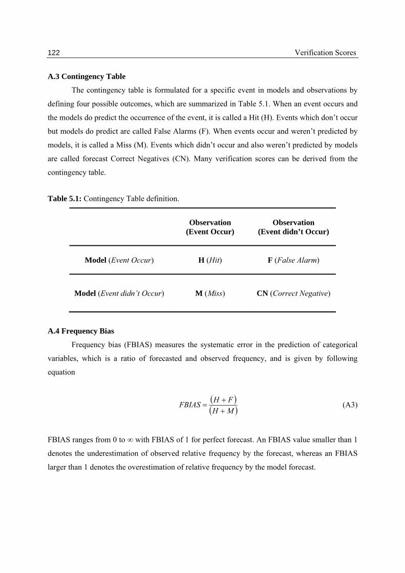
122 Verification Scores
A.3 Contingency Table
The contingency table is formulated for a specific event in models and observations by
defining four possible outcomes, which are summarized in Table 5.1. When an event occurs and
the models do predict the occurrence of the event, it is called a Hit (H). Events which don’t occur
but models do predict are called False Alarms (F). When events occur and weren’t predicted by
models, it is called a Miss (M). Events which didn’t occur and also weren’t predicted by models
are called forecast Correct Negatives (CN). Many verification scores can be derived from the
contingency table.
Table 5.1: Contingency Table definition.
Observation
(Event Occur)
Observation
(Event didn’t Occur)
Model (Event Occur) H (Hit)
F (False Alarm)
Model (Event didn’t Occur) M (Miss)
CN (Correct Negative)
A.4 Frequency Bias
Frequency bias (FBIAS) measures the systematic error in the prediction of categorical
variables, which is a ratio of forecasted and observed frequency, and is given by following
equation
MH
FHFBIAS
(A3)
FBIAS ranges from 0 to ∞ with FBIAS of 1 for perfect forecast. An FBIAS value smaller than 1
denotes the underestimation of observed relative frequency by the forecast, whereas an FBIAS
larger than 1 denotes the overestimation of relative frequency by the model forecast.

123 Verification Scores
A.5 Equitable Threat Score
The equitable threat score (ETS, [Schaefer, 1990]) measures the accuracy of a correct
forecast at a certain time and station for categorical variables, which is given by following
equation
RAN
RAN
HFMH
HHETS
, (A4)
where HRAN is number of hits by chance. ETS ranges from -1/3 to 1, where ETS value of smaller
than zero indicate no skill where ETS of 1 is representative of perfect forecast.
A.6 Spread and RMSE for Ensemble
The ensemble spread is calculated by measuring the deviation of ensemble forecasts from
their mean [Zhu, 2005], which is defined as below:
M
nn tftf
MtSpread
1
2
)()(1
1)( , at time t (A5)
where
M
nn tf
Mtf
1
)(1
)( is ensemble mean and fn’s are their ensemble members, where M is the
number of ensemble members.
The ensemble root mean square error (RMSE) is the distance measured from the ensem-
ble mean to the observation, which is given by the following equation
N
n
nofN
RMSE1
2
)(1
1 (A6)
where
M
nn tf
Mtf
1
)(1
)( is the ensemble mean and O’s are observations and N is available
forecast observation pairs.

124 Verification Scores
A.7 Rank Histogram
Rank histogram [Anderson, 1996; Talagrand et al., 1997; Hamill, 2001] is a useful
measure of reliability [Hou et al., 2001; Candille and Talagrand, 2005] of an EPS. The rank
histogram is calculated by sorting all m ensemble forecasts plus verifying observations. Then the
rank of the observations is determined with respective to the ensemble forecasts, and finally a
rank histogram is calculated as the sum of all individual ranks within the verification period and
stations or grid cell. In a perfect ensemble system, distribution of every single forecast is similar
to the distribution of the observations. In other words, statistically, the observations and every
individual ensemble members are indistinguishable. This leads to a flat-rank histogram (Figure
A1a). EPS with insufficient spread forces the observations to be outliers, which are accumulated
in the first or last bin of the histogram leading to a U-shaped histogram (Figure A1b). Over
dispersive ensemble systems with too-large spreads compared to the observations exhibit a bell
shaped histogram (Figure A1c). The EPS with positive biases exhibit positively skewed (Figure
A1d) and with negative bias exhibits negatively skewed histograms (Figure A1e) as it ranks
observational truth to the first or last rank respectively.
Candille and Talagrand [2005] proposed to measure the deviation of the rank histogram
from flatness for an EPS with M members and N available forecast observation pairs with the
following procedure: The number of values in each bin of the rank histogram is given by Si. For
a reliable ensemble system with a flat histogram, Si is equal to N / (M +1). Then
21
1 1
M
ii M
NS
measures the deviation of the histogram from the flatness. For perfect reliable ensemble systems,
the base value is defined as
)1(0
M
NM
So the ratio 0
(A7)
is the overall flatness of the rank histogram. A value of δ that is significantly larger than 1
indicates the system does not reflect equal likelihood of ensemble members.

125 Verification Scores
Figure A.1: Hypothetical ranked histograms for a 10 member EPS system. a) For perfect EPS,
b) for EPS with insufficient spread, c) for over dispersive ensemble systems d) for EPS with
positive bias, and e) for EPS with negative bias.
A.8 Brier Score and Brier Skill Score
The Brier score is defined as the mean square error of the probabilistic forecast, and it is
one of the most widely used EPS evaluation scores [Brier, 1950]. The Brier score is designed to
quantify the performance of a probabilistic forecast of a dichotomous event. It is given by the
following equation:
N
Kkk OP
NBS
1
21 , (A8)
where N is the number of forecasts, Pk is the forecast probability (fraction of ensemble members
that exceed threshold), and Ok is the verifying observation (equal to 1 if the observation exceeds
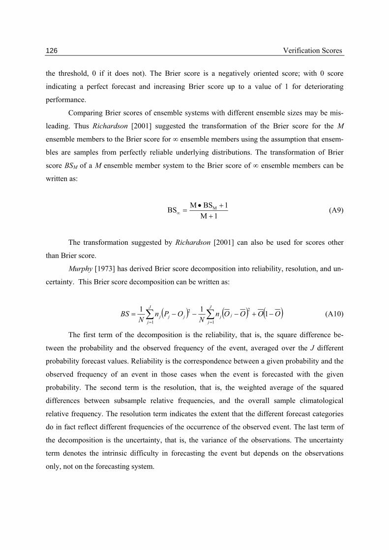
126 Verification Scores
the threshold, 0 if it does not). The Brier score is a negatively oriented score; with 0 score
indicating a perfect forecast and increasing Brier score up to a value of 1 for deteriorating
performance.
Comparing Brier scores of ensemble systems with different ensemble sizes may be mis-
leading. Thus Richardson [2001] suggested the transformation of the Brier score for the M
ensemble members to the Brier score for ∞ ensemble members using the assumption that ensem-
bles are samples from perfectly reliable underlying distributions. The transformation of Brier
score BSM of a M ensemble member system to the Brier score of ∞ ensemble members can be
written as:
1M
1BS MBS M
(A9)
The transformation suggested by Richardson [2001] can also be used for scores other
than Brier score.
Murphy [1973] has derived Brier score decomposition into reliability, resolution, and un-
certainty. This Brier score decomposition can be written as:
OOOOnN
OPnN
BS j
J
j
J
jjjjj
111 2
1 1
2 (A10)
The first term of the decomposition is the reliability, that is, the square difference be-
tween the probability and the observed frequency of the event, averaged over the J different
probability forecast values. Reliability is the correspondence between a given probability and the
observed frequency of an event in those cases when the event is forecasted with the given
probability. The second term is the resolution, that is, the weighted average of the squared
differences between subsample relative frequencies, and the overall sample climatological
relative frequency. The resolution term indicates the extent that the different forecast categories
do in fact reflect different frequencies of the occurrence of the observed event. The last term of
the decomposition is the uncertainty, that is, the variance of the observations. The uncertainty
term denotes the intrinsic difficulty in forecasting the event but depends on the observations
only, not on the forecasting system.
127 Verification Scores
The Brier score can be converted to a positively oriented skill score, as
refBS
BS1 BSS (A11)
The skill of a reference system (BSref) is often taken to be a simple climatological fore-
cast in which the probability of the event always is equal to O for all the forecasts. The Brier
score for such climatological forecasts is OOBSref 1 , then the Brier skill score can be
expressed as
(A12)
yreliabilit relativeresolution relative BSS
As BSS is positively oriented score, the perfect forecast will have the BSS value of 1. A
perfect forecast would have a relative resolution equal to 1 and a relative reliability equal to 0.
After Richardson [2001] adjustment for the ensemble size, the BSS can be written as:
1
1
1
1
M
BSSM
M
BSSMBSS MrelrelibMrelres (A13)
A.9 Continuous ranked probability score
The continuous ranked probability score (CRPS) defined in Stanski et al. [1989]
measures the global skill of the ensemble forecast. CRPS measures the distance between the
predicted and the observed cumulative density functions (CDFs) of scalar variables. The CRPS is
given by the following equation
dxxFxFCRPS OP
2
)()(
, (A14)
where FP and FO are the predicted and observed CDFs respectively over all possible realizations
(over all stations or grid cell for whole period). The CRPS has the dimension of the predicted

128 Verification Scores
variable. The CRPS is negatively oriented, reaching its minimum value of zero for a perfect
deterministic system. Larger values of the CRPS indicate lower skill of the EPS. It is the general-
ization of the Brier score [Brier, 1950] over all the possible thresholds of the variable under
consideration.
Similar to the Brier score, the CRPS scores also can be decomposed into reliability, reso-
lution and uncertainty component [Hersbach, 2000]. The CRPS score decomposition is written
as follows
CRPS = Reli – CRPSpot , (A15)
where,
CRPSpot = Resol + Unc , (A16)
N
0i
2iii )po(gReli , (A17)
)o1(ogCRPS i
N
oiiipot
, (A18)
where N is the ensemble size, gi is the average width of the bin I (Euclidean distance between
consecutive ensemble members), oi can be seen as the average frequency that the observation is
less than the middle of the bin i, and pi is the fraction i/N. The Reli component measures the
reliability of the EPS, whereas CRPSpot measures the difference between the resolution of the
EPS and the uncertainty associated with the variable considered. The uncertainty term does not
depend on the prediction system, thus CRPSpot corresponds only to the resolution of EPS. Like
the CRPS, its two components are also negatively oriented [Hersbach, 2000], that is, the smaller
those scores are, the better the EPS. The Reli is equal to 0 for perfectly reliable systems, while
distance from 0 is indicative of the lack of reliability. Reli measures the average reliability of the
ensemble forecasts; it tests whether the fraction of observations that fall below the kth of n ranked
ensemble members is equal to k/n on average. For perfect deterministic systems, the CRPSpot
reaches its minimum, while positive values indicate the lack of resolution. It is sensitive to the
average ensemble spread and the frequency and magnitude of the outliers. For the best potential
129 Verification Scores
CRPS, the forecasting system needs a narrow ensemble spread on average without too many and
extreme ensemble outliers [Hersbach, 2000].
A.10 Reliability Diagram
The reliability of forecasts is often represented by the reliability diagram (Figure A.2)
which is a diagram between the observed relative frequency and the forecasted probability for
the particular thresholds corresponding to the forecast event [Wilks, 1995; Toth et al., 2003]. The
reliability diagram is used to test the ability of the system to correctly forecast probabilities of a
certain event. A reliability diagram is created by binning the continuous forecast probability
values into discrete, contiguous bins of probability, then plotting the forecast probability at the
center of each bin against the corresponding observed relative frequency. For the ideal forecast,
the probabilistic forecast observation points lie on the diagonal of the reliability diagram, indicat-
ing the event is always forecasted at the same frequency as observed. The Brier score reliability
component is a weighted-squared distance between the reliability curve and the diagonal line.
The reliability curve above the diagonal indicates the under forecast, while below the di-
agonal indicates the over forecast. The reliability curve centered on the diagonal with smaller
deviations represents very good reliability, as small deviations are mostly due to the small
sample size. The sharpness diagram is usually plotted with the reliability which characterizes the
relative frequency of occurrence of the forecast probabilities category. The sharper EPS will
have forecast probability frequently near 0 or 1, which indicates the forecasts deviate significant-
ly from the climatological mean, a positive attribute of an ensemble forecast system. Sharpness
measures the variability of the forecasts alone, and in a perfectly reliable forecast system sharp-
ness is identical to resolution.

130 Verification Scores
Figure A.2: Hypothetical reliability diagrams, (a) for climatological EPS forecast, (b) for EPS
forecast with minimal resolution, (c) for a EPS forecast with underestimation, (d) represents
a EPS forecast with good resolution but poor reliability, (e) for rare event, and (f) for small
EPS sample size. The inset shows sharpness diagrams.

131 Verification Scores
A.11: ROC diagram and ROC area
The Relative Operating Characteristic (ROC) curve measures the discrimination of the
EPS, which reflects the ability to distinguish between the occurrence and non-occurrence of
forecast events. It is the converse of resolution, in other words discrimination measures the
sensitivity of the probability that an event was forecasted, conditioned on whether or not the
event was observed. The ROC curve is a verification measure based on signal detection theory
which Mason [1982] first introduced in meteorology. The ROC is a graph of the hit rate (HR)
against the false alarm rate (FAR) for specific decision thresholds. The hit rate and false alarm
rate is derived from the contingency table by the following equations:
MH
HHR
(A19)
CNF
FFAR
. (A20)
The ROC measure is based on the stratification by observations and, therefore, is independent of
reliability, and instead provides a direct measure of resolution. The perfect discrimination is
represented by an ROC curve (Figure A.3a) that rises from (0,0) along the y axis to (0,1), and
then horizontally to the upper-right corner (1,1). The diagonal line from (0,0) to (1,1) represents
zero skill, indicating no discrimination among events by forecasts. The real world forecast lies in
between these two extremes (Figure A.3b). Forecasts with better discrimination exhibit ROC
curves approaching the upper-left corner of the ROC diagram more closely, whereas forecasts
with very little ability to discriminate the event exhibit ROC curves very close to the HR = FAR
diagonal (Figure A.3c).
The area under the ROC curve is widely used as a verification measure of the forecast
resolution. The ROC area can be calculated by the trapezoidal rule or binormal method [Mason,
1982; Swets, 1986]. The trapezoidal rule is the correct method to calculate the ROC area for
small sample sizes; however, this can lead an underestimation for large sample sizes [Wilson,
2000]. We have used the binormal method to calculate the ROC area, as we have a large enough
sample size. Since ROC curves for perfect forecasts pass through the upper-left corner, the area
under a perfect ROC curve includes the entire unit square, so Aperf = 1. Similarly, ROC curves

132 Verification Scores
for random forecasts lie along the 45o diagonal of the unit square, yielding an area Arand = 0.5.
The area A under a ROC curve of interest can be expressed in standard skill score as
ROCSS = 2 ROC Area -1 (A21)
An ROCSS of 0 indicates the no-skill forecast, whereas 1 represents perfect discriminating
forecasts.
Figure A.3: Hypothetical ROC diagrams, a) for perfect case, b) realistic case c) for EPS forecast
having same skill as climatological mean, d) for EPS forecast worse than climatological
mean.

133 Verification Scores
A.12 Forecast value
The usefulness of the ensemble forecast for different decision-making processes can be
evaluated based on the simple cost-loss model proposed by Richardson [2000]. This model uses
a contingency table to calculate the forecast value based on the hit and false alarm rate similar to
a ROC curve. The hits and false alarms both incur a cost of taking preventative action (C).
Misses are associated with a loss due to the lack of prevention (L). Correct rejections incur no
expenses either way. Thus the economic values (V) of the forecasts are defined in terms of
expenses, E, in an equivalent manner as skill scores for meteorological forecasts [Richardson,
2003].
perfectclimate
forecastclimate
EE
EEV
(A22)
The decision using the climate frequency of the event can be done in two ways: 1.) always take
protective action, thus incurring a constant cost C but never experiencing a loss L, or 2.) never
take protective action, which involves no cost but will result in total losses equivalent to OL,
where O is the climatological probability of the event occurring. This means the expense for the
climatological frequency Eclimate is min(C, OL). For the perfect forecast, the decision maker will
take action when the event occurs; therefore, it would only incur costs at the climatological base
rate. The mean expense would then be Eperfect = OC.
The sample mean expense of the forecast is calculated by multiplying the relative frequencies of
each of the four possible outcomes of the contingency table for a specific threshold by the
corresponding expense, resulting in
Ln
MC
n
FC
n
HE forecast , (A23)
where n = H + F + M + CN is the total number of forecast observation pairs. Thus, the economic
value Equation can be written as
rOOrn
MFH
n
rOr
V
),min(
)(),min( , (A24)

134 Verification Scores
where r = C/L is the specific user’s costloss ratio. Using hit rate (HR), false alarm rate (FAR)
and climatological base rate O = (H + M)/n, the equation for economic value V can be rewritten
as
rOOr
OrOHRrOFAROrV
),min(
)1()1(),min( . (A25)
The only optimal ensemble forecast value is considered which gives the maximum possible
values for the each cost-loss ratio. The maximum value occurs at that value of C/L equal to the
climatological base rate O.

135
Appendix B
Significance Test
The methods used to infer the significance of the result gained from the limited sam-
ple are explained in this appendix. Forecast verification is often based on the investigation of
different properties of the joint probability distribution of forecasts and observations. In this
study we have compared the skills of the different model forecasts with each other. Because
of the finite number of forecast / observation pairs, statistical significance of the result should
be given. A number of hypothesis tests and confidence intervals are available; however, they
are based on different assumptions. Hypothesis testing for significance can be categorized
into parametric and nonparametric tests. Parametric tests assume a particular theoretical
distribution representing the data, while, for nonparametric tests, such an assumption is not
required. Parametric tests are particularly used when the analysis are based on particular
distribution parameters. However, parametric tests (such as t test) are based on several
conditions, such as the data being tested are independent samples, and the data are normally
distributed and have equal variances. As a nonparametric test does not consider the theoreti-
cal distribution of the data, the condition of the normality of data is relaxed for the nonpara-
metric test; however, the other two conditions are still required. Nonparametric tests also can
be categorized in classical nonparametric and resampling tests. The classical nonparametric
tests consider the distribution of the data to be unimportant and thus can be used for data with
any distribution. In resampling tests, the distribution of the data can be inferred from the data
by repeated computer manipulations. The different approaches used in forecast verification
studies to test the significance of the results are discussed by Jolliffe [2007]. Mason [2008]
gives a detailed overview of the interpretation of verification statistics with their significance.
As most of the atmospheric water cycle variables considered for the verification are non-
Gaussian, the significance of the result is tested with the non parametric test. The following
section will introduce the classical and resampling nonparametric tests used in this study.
B.1 Wilcoxon-Mann-Whitney rank-sum test
The Wilcoxon-Mann-Whitney rank-sum test was devised independently in the 1940s
by Wilcoxon, and by Mann and Whitney [Mann and Whitney, 1947]. The independence of
two samples is tested based on their rank. As the ranking of the data is considered, outlier
data points will not have any impact on the result. To test whether both the samples are drawn

136 Significance Test
from the same distribution, the mean and median of their ranked data distribution is tested.
The null hypothesis is that the two data samples drawn from the same distribution, and the
alternative hypothesis is that the two sample distributions differ. If the null hypothesis of
identical population distributions is true, then n1 ranks from the population are just a random
sample from the N integers 1,.,.,.,., N. Thus, under the null hypothesis, the distribution of the
sum of the ranks ‘T’ depends only on the sample sizes, n1, and n2, and does not depend on
the shape of the population distributions. Under the null hypothesis, the sampling distribution
of T has mean and variance given by
2
)1( 211
nnnT and (B.1)
12 21
212 nnnn
T . (B.2)
Intuitively, if T is smaller than the 0.05 significance level, then μT provides evidence that the
null hypothesis is false and in fact the population distributions are not equal. The rejection
region for the rank sum test specifies the size of the difference between T and μT for the null
hypothesis to be rejected.
B.2 Bootstrap method
The bootstrap method infers the statistical significance of the data from the data them-
selves, which was invented by Efron [1979]. Bootstrap treats the finite sample similar to the
unknown distribution from which it is drawn. The bootstrap sample is created by choosing N
random samples from the original data set, with replacements. So within a bootstrap sample,
an original value may appear more or less often in the data set or even not all. This artificially
represents the fact that the data set itself is only a finite sample from the true distribution. The
number of samples has a significant impact on the result: if sample number is very small, all
samples can be fully enumerated. Thus, a bootstrap sample of 1000 or more is required to test
the significance of the results. Time series with non-negligible autocorrelation can be dealt
with by autoregressive schemes, and the corresponding parameters are bootstrapped with the
disadvantage that first an appropriate model has to be chosen. This can be omitted by consid-
ering the autocorrelation of a time series in a nonparametric bootstrap procedure. Instead of
creating the bootstrap samples by resampling every value, one chooses whole blocks of
appropriate length out of the time series and puts them together to gain a bootstrap sample

137 Significance Test
time series. As the block width depends on the autocorrelation, it should be large enough that
the blocks are nearly independent but not too large in order to keep the bootstrap mechanism
efficient. Block width of 24 hours are considered by testing the autocorrelation for all key
variables; all variables show very small autocorrelation at 24 hours. Significance of the result
is tested by the median-to-interquantile ratio (M2I), which is calculated by dividing the
median value of the distribution by half the interquantile distance of the 95% quantile minus
the 5% quantile. M2I is a measure of the median difference of the scores for the two models
as compared to the width of the difference distribution specified by the resampling. The
higher value of M2I is representative of the significant differences in the scores.

138 Significance Test