1

DIASTOLIC BLOOD PRESSURE, CARDIOVASCULAR DISEASE, and MORTALITY

Sidney Port, Linda Demer, Robert Jennrich, Noel Boyle, Alan Garfinkel

Departments of Mathematics (S Port PhD), Statistics (S Port, R Jennrich PhD),

Medicine-Cardiology (L Demer MD PhD, N Boyle MD PhD, A Garfinkel PhD), Physiology

(L Demer) and Physiological Science (A Garfinkel), University of California, Los Angeles,

CA

Prepublication management

Noel BoyleUCLA School of MedicineDivision of CardiologyRoom 47-123 CHS10833 LeConte AvenueLos Angeles, CA 90095-1679Phone: 310-794-2165Fax: 310-206-9133Email: nboyle@mednet.ucla.edu

Correspondence to:

professor Sidney Port

Department of Mathematics

University of California, Los Angeles

Los Angeles, CA. 90025

(e-mail:sport@ucla.edu)

2

Summary

Background There are two views of the relation between diastolic blood pressure and

risks of cardiovascular disease and death. The most widely accepted is that risk is

steadily rising with diastolic blood pressure. The other is that the relation follows a “J-

curve”, in which risks are also increased at low as well as high pressures. This view is

controversial because it is not consistently found. We reanalyzed data from the

Framingham study to determine the nature of the relation of cardiovascular risk to

diastolic blood pressure, to see why the J-curve is elusive, to seek justification for taking

90 mm Hg as the cut-point for diastolic hypertension, and to determine if the systolic or

diastolic pressure is a better predictor of risk.

Methods Reanalysis of the Framingham data on diastolic blood pressure using

logistic splines.

Results & Interpretations (1) The Framingham data rejects the linear logistic model;

the risk - diastolic blood pressure relation is not continuous and strictly increasing. (2) The

basic relation of risk to diastolic blood pressure is the same as we previously found for

systolic blood pressure, namely risk is constant to a threshold at the 70th percentile

pressure (about 90 mm Hg) and steadily increases thereafter. (3) Rather than being

arbitrary, 90 mm Hg is a natural threshold for hypertension.(4) The J-curve phenomenon

is a barely detectable effect, hovering on the boundary of statistical significance, that may

cause a rise in risk for pressures less than 70 mm Hg. The weakness of this effect may

explain why its detection is so elusive (5). Systolic blood pressure and diastolic blood

pressure are equivalent predictors of risk. (6) For the soft endpoint of cardiovascular

disease incidence there is a sharp jump at 90 mm Hg, with risk being constant to the left

of 90 mm Hg, again constant between 90 mm Hg and 104 mm Hg, and a increasing

thereafter. The difference between this outcome and the ‘hard’ outcomes suggests that

the presence or absence of hypertension may influence the diagnosis of cardiovascular

disease.

3

INTRODUCTION

Both JNC VI 1 and WHO/ISH 2 support the view that the relation of both diastolic and

systolic blood pressure to endpoints such as death due to cardiovascular disease is

continuous, strictly increasing, and with no lower bound (Fig. 1). This, they say, is based

on the preponderance of eveidence from epidemiological studies and randomized trials.

Previous analysis from the Framingham study 3,4 was instrumental in propagating this

view of the risk - blood pressure relation, primarily by the use of linear logistic smoothing

of the data. We previously reported that the relation between cardiovascular risks and

systolic blood pressure was not linear but has a threshold level 5. Risk was not increased

at any pressures except for those in the upper 30% of pressure for their age and sex. We

also found that the use of 140 mm Hg as the universal division between normal and

elevated systolic blood pressure was unjustified; it needed to be replaced by age and sex

dependent cut-points.

Unlike the case with systolic pressure, there has long been some opposition to the

strictly increasing model of cardiovascular risk with diastolic blood pressure. Starting with

Andersen’s observation 6 that the same Framingham data considered here apparently

showed that the risk of cardiovascular disease decreases (rather than increases) with

increasing diastolic pressure to 89 mm hg, this controversy has centered on the “J-curve

effect”. That effect is an apparent increase in risk at low as well as high diastolic blood

pressure 6-21. This view is controversial, primarily because it is not consistently found.

We reassessed the diastolic pressure data from the Framingham 18 year follow up

report 4 for the following outcomes: cardiovascular disease incidence, death due to

cardiovascular disease, and overall mortality. Our primary goal was to determine the

nature of the relation of these risks to diastolic blood pressure. Secondary goals were to

explain why the J-curve effect was so elusive, to see what justification there was for 90

mm Hg being a universal cut-point for diastolic hypertension, and to find whether the

diastolic blood pressure or systolic blood pressure was a better predictor of risk.

We chose to reanalyze the Framingham 18-year follow up data because: (10 it was

accurately gathered, (2) it was unconfounded by antihypertensive drug intervention, (3) it

contained women, (4) it contained older people.

4

Methods

The Framingham data 4 are presented separately for each sex divided into three age

groups 45-54, 55-64, and 65-74 years. There are 10 blood pressure categories (Table 1)

Unlike the systolic pressures, for persons aged 45-74, the distribution of diastolic

pressures does not change much with age and is about the same in both sexes For

practical purposes we can take these distributions to be the same.

We first determined if the relation of overall and cardiovascular disease death to

diastolic blood pressure is homogeneous across the six groups, i.e. if the additive model

holds. In that model the risk for a person is simply the sum of two effects, one based on

the group the person is in and the other from the person’s blood pressure. Our analyses

were carried out using both the specific rates and the direct group adjusted rate. Models

for the specific rates were viewed as sub-models of the additive model.

We modeled the relation of both overall and cardiovascular death to diastolic blood

pressure by curves known as logistic splines. A logistic spline is a curve that results from

continuously joining two or more logistic curves. The points where two curves join are

called knots and the curves are called segments. A logistic spline is parameterized by the

location of the knots, an intercept term, and a slope term for each segment. A segment

with slope 0 is a horizontal line. In all our models the knots are specified in advance and

in some models some of the segments are specified to have 0 slope. Consequently, the

number of unknown parameters is 1 + (number of slope terms ≠ 0).

A 2-spline is a logistic spline curve having two knots, which we will label the left knot

and the right knot, and 3 segments. These are a left segment (from the left endpoint to

the left knot), a middle segment (from the left knot to the right knot), and a right segment

(from the right knot to the right endpoint). A horizontal 2-spline is a 2-spline where the

middle segment has 0 slope (i.e. is a horizontal line). A 1-spline has 1 knot and two

segments, viz. left and right. A horizontal 1-spline is a 1 spline whose left slope is 0.

Models based on the specific rates required one curve for each age group. Because

all models were sub-models of the additive model, these curves had to be parallel.

Therefore, they all had the same knots, and for each of the six curves, the corresponding

segments had a common slope.

5

We previously modeled the relation of cardiovascular disease death to systolic blood

pressure 5 by a horizontal 1-spline with its knot at the 70th percentile pressure. The salient

feature of the J-curve effect is the downward trend in the risk as pressures move from the

lowest value to more moderate values. We used 2-spline models both to determine if

there was a significant J-curve effect and to model it if it was significant. The knots were

chosen to produce a model as close as possible to that for the relation of cardiovascular

disease death to systolic blood pressure and still allow the possibility for a J-curve effect.

Therefore, we chose the right knot at 90 mm Hg and left knot as far to the left as possible.

We took the left knot to be the left endpoint of the second lowest class, namely 70 mm

Hg. [However, the fit would have been the same for any choice between 67 mm Hg and

72 mm Hg]. In addition to this model we also fitted a horizontal 2-spline with the same

knots, and a horizontal 1-spline with its knot at 90 mm Hg. For all models, tests for

significance of the slopes of the various segments were done.

The parabolic model consists of logistically fitting a parabola to either the adjusted

rates or six parallel parabolas to the specific rates. We also considered parabolic models

for both the relation of overall and cardiovascular death to systolic blood pressure.

Various tests were performed based upon this model to see if a parabolic relation is real.

Parabolic and spline models were compared.

For the relation of incidence of cardiovascular disease to systolic blood pressure we

needed to consider a model called the jump model. The jump curve consists of a

horizontal line from the initial pressure to 90 mm Hg and a separate horizontal 1-spline

with initial point at 90 mm Hg and knot at 104 mm Hg. Such a curve has a jump at 90 mm

Hg. The jump model on the specific rates consists of six parallel jump curves. We used

the goodness of fit test to see if various models (linear logistic, 1-spline, 2-spline,

parabolic, and jump) fit the data.

Two methods were used to compare the predictive ability of systolic blood pressure to

that of diastolic blood pressure for cardiovascular death. The first was to compare their

error sums of squares. The second was to compare their standardized right slopes.

6

Results

Analyses using the specific rates and the adjusted rates yielded the same results.

The logistic model does not hold

The goodness of fit test soundly rejected the linear logistic model ("p-value" < 0.001

for both the specific rates and the adjusted rates).

The relation of cardiovascular death to diastolic blood pressure.

The 2-spline model gave an excellent fit ( "p-value" = 0.821 specific rates, 0.800 for

the adjusted rates). Examining the slope terms showed three things: (i) The middle slope

could be taken to be 0 ("p-value" = 0.90 specific rates, =0.802, adjusted rates). (ii) The

right slope was highly significant ("p-value" = 0.001 specific rates, = 0.002 adjusted rates).

(iii) The left slope was almost significant ("p-value" =0.060, specific rates, = 0.104

adjusted rates). Consequently, use of the horizontal 2-spline model was warranted. As

judged by the goodness of fit test the horizontal 2-spline model (figure 2) was excellent

("p-value" for fit = 0.900, specific rates, "p-value" for fit = 0.874 adjusted rates). The right

slope was again highly significant ( "p-value" < 0.001 for both the specific and adjusted

rates). But now, the left slope was also significant ("p-value" = 0.019 for the specific rates

and 0.053 for the adjusted rates). The horizontal 1-spline (figure 2) also gave a good fit

("p-value" for fit =0.443 specific rates, = 0.551 adjusted rates). Consequently, there were

two choices for the model of the relation of cardiovascular disease death to systolic blood

pressure (viz. the horizontal 1- spline and the horizontal 2-spline) one excluding and the

other including the J-curve effect. These are virtually identical (figure 2) except for the

behavior at pressures below 70 mm Hg.

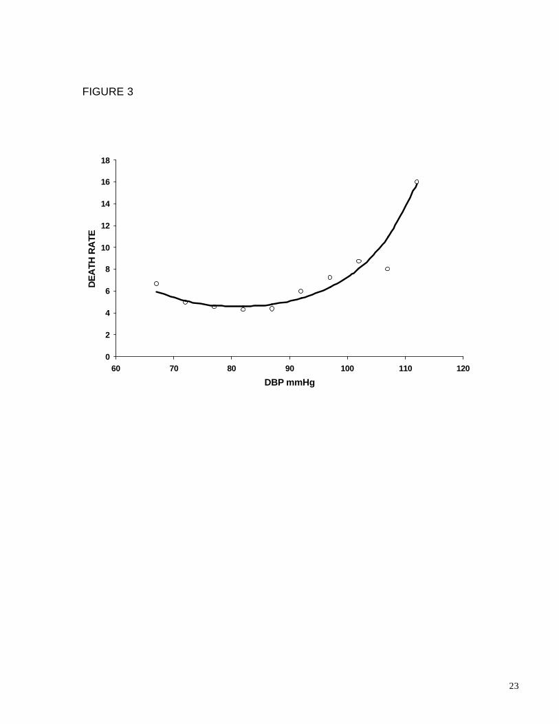
Previous investigators 9 have represented the J-curve effect by the parabolic model.

The goodness of fit test showed that the parabolic model (figure 3) also provides a good

fit to the Framingham data (p- value for fit = 0.827, specific rates = 0.872, adjusted rates).

That model implies that there is a unique diastolic blood pressure at which risk is a

minimum, ( = 81.4mm Hg) with risks smoothly increasing away in both directions from

that point (figure 3). However, comparing the horizontal 2-spline and the parabolic models

we found that the parabolic model had two serious statistical drawbacks: First, the entire

statistical significance of the downward trend to the minimum was due to the leftmost

7

point. Excluding that point, the test for trend to pressure 82 mm Hg showed there was no

significant downward trend ("p-value" for slope = 0.385 using specific rates, "p-value" for

slope = 0.485 using adjusted rates). Second, it implied that the risks were continuously

increasing for pressures past 81.4 mm Hg. However, the entire significance of the

increase came from pressures past 90 mm Hg. A test for tend to pressure 90 mm Hg

excluding the leftmost point showed there was none ("p-value" for slope = 0.444 specific

rates, = 0.509 adjusted rates). The parabolic model tries to approximate this flat portion,

producing a somewhat abnormal residual pattern compared to the horizontal 2-spline

(See figures 2 and 3).

The relation of cardiovascular Disease Incidence to diastolic blood pressure

Heretofore, the relation of incidence of cardiovascular disease to diastolic blood

pressure has been modeled primarily by the use of adjusted rates using either the linear

logistic or the parabolic model. As for cardiovascular disease death, the additive model

was valid for the relation between incidence of cardiovascular disease and diastolic blood

pressure ("p-value" = 0.864) and the linear logistic model was rejected ("p-value" < 0.001

for both the adjusted and specific rates).

The adjusted incidence of cardiovascular disease rates investigated here are the

same data used by Andersen 6 when he found that the risks to pressure 89 mm Hg had a

downward slope. However, he did not determine if this slope was significant. The test for

trend to this pressure showed that it was not significant ("p-value" = 0.381, adjusted rate,

"p-value" = 0.351,specific rate). The parabolic model was rejected ("p-value" for fit =

0.008 for both rates). The 1-spline model was rejected ("p-value" = 0.014 group specific

rates, "p-value" = 0.015 adjusted rates) as was the 2-spline ("p-value" ≤ 0.01 for both

rates). Thus all models previously used for relations of cardiovascular risk to diastolic

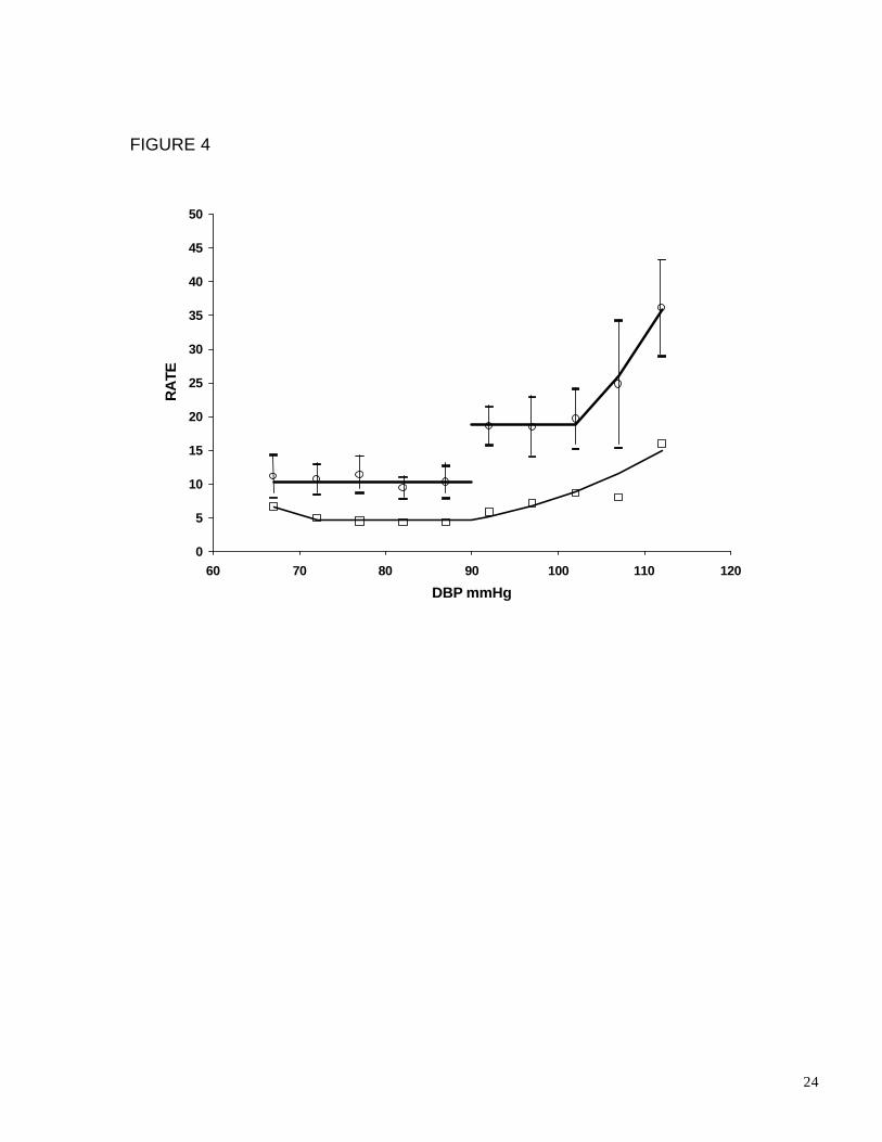
blood pressure were rejected by these data. On the other hand, the jump model (figure 4)

fitted very well ("p-value" for fit = 0.889 specific rates, "p-value" = 0.937, adjusted rates).

Tests of the significance of the jump and of the significance of the slope past 104 shows

both were highly significant ("p-value" < 0.001 for both specific and adjusted rates for both

coefficients). The magnitude of the jump is impressive [odds ratio of risk to left of 90 to

risk just past 90 = 1.828 CI (1.312,2.344), specific rates, odds ratio = 1.869 CI

(1.346,2.407) adjusted rates].

8

Predictive ability of diastolic versus systolic blood pressure

Strictly speaking, as judged by the error sums of squares, either of the two diastolic

pressure models yielded better predictions of cardiovascular death than did the systolic

model ("p-value" for fit: diastolic pressure horizontal 2-spline = 0.945, diastolic pressure

horizontal 1-spline = 0.850, systolic pressure horizontal 1-spline = 0.7026). Comparing

the standardized right slope in the either of the diastolic models to the right slope in the

systolic model showed that there was no significant difference between these slopes.

[From our data we could only obtain a rather poor lower bound for the standard error of

the difference between the two standardized estimates. This considerably overestimated

the exact z-score, but sufficed to show that there was no significant difference between

them ("p-value" ≥ 0.118)].

9

DISCUSSION

There are currently two of theories the relation between diastolic blood pressure and

such endpoints as death due to cardiovascular disease, overall mortality, and incidence of

cardiovascular disease. The paradigm 1,2 is that the relation is modeled by the linear

logistic curve and therefore risk is strictly increasing with pressure.

The Framingham 18-year study data 4 was instrumental in establishing this paradigm.

Our reanalysis of these data show that it statistically rejects the linear logistic model for

any of these outcomes. This single fact has much broader implications than might first be

assumed because it, in and of itself, proves that the paradigm is false. Although

numerous studies are needed to build confidence that the model may be valid, no number

of studies can ever prove that the model is true. In contrast, finding just a single study,

that is based on a representative sample from its target population, that statistically

rejects the linear logistic model for the risk-diastolic blood pressure relation will definitively

prove that the paradigm is false for its target population. Consequently, any study of

sufficiently large size that fails to reject the paradigm must either be a sample from a quite

different population or it must be seriously biased. Therefore, granting that the

Framingham data does constitute a representative sample from its target population

(white, urban, middle class Americans) the relation of risk to diastolic pressure in that

population is not continuous and strictly increasing for any of the risks investigated here.

The second view is that the relation is given by a “J-curve” in which risks increase with

low as well as high pressure. Since its beginnings with Andersen 6 and Stewart 7 this view

has been controversial, and the entire J-curve issue is confusing. The causes of this

phenomenon and even its existence have been vigorously debated. The phenomenon is

found in many, but not all, observational studies and clinical trials 7-21. It is found more

frequently in studies including older persons or those with ischemic heart disease,

although it is found in some studies that contain neither 21. In the main, those studies that

fail to exhibit the J-curve phenomenon analyze the data by linear logistic smoothing 11.

This of course would obliterate any trace of the phenomenon. In some studies the J-curve

phenomenon was found to hold for incidence as well as cardiovascular death and overall

mortality 11. For others it was found to be present only for death (either all causes, due to

10

cardiovascular disease, or due to coronary heart disease). Some studies find that it

occurs only for those with previous ischemia or with previous myocardial infarction. Most

of the studies that did not exclude those with previous ischemia showed the J-curve

phenomenon 18. In contrast, several studies that did exclude those with ischemia did not

show this phenomenon 20. Other studies find it present even for those without previous

ischemia 10. The strongest case to date for the linear logistic relation of diastolic blood

pressure to various risks is by MacMahon et al 12,13 . There have been counter arguments

to their methods of analysis and conclusions14 – 16.

If there is a J-curve effect, its causes are open to considerable speculation 18, 19. One

suggested cause is anti-hypertensive medication. This would seem to be contradicted by

the fact that the J-curve phenomenon occurs in studies such as the early Framingham

data discussed here, that are relatively free of drug intervention. Coope 21 classifies the

two main hypotheses about causation as direct and reverse causation. The former, first

suggested by Green 20, 21, is that it is due to coronary ischemia, as diastolic blood

pressure drops below some critical value needed to preserve perfusion of the

myocardium. If that is the case, then there could well be a critical value of low diastolic

blood pressure such that flow is seriously impaired for pressures below that value, but not

for pressures above that value. The latter claims that the low diastolic blood pressure is a

marker for some preexisting condition.

Until now, whenever modeled, the J-curve effect has been represented as a parabolic

type relation between risk and diastolic blood pressure. We believe that such a view is

both misleading and not supported by the facts. A parabolic representation portrays the J-

curve effect as a steady increase in risk in both directions from a unique point of minimum

risk (figure 3). However, our analysis shows that for all adults ages 45-74, there is a large

interval of diastolic blood pressure (at least from 70 mm Hg to 90 mm Hg) in which the

risks are constant and only begin to rise for pressures above a threshold at 90 mm Hg.

There may also be a lower threshold at about 70 mm Hg with risks again rising for

pressures below that threshold. Another shortcoming of the parabolic model for the

relation of either overall mortality or cardiovascular death to diastolic blood pressure is

that it implies that that relation is entirely different than it is for the relation of these risks to

systolic blood pressure. This is difficult to understand since, based on data in the national

11

health examination survey,22 the two pressures are on average 84% correlated. In

particular, it is difficult to understand why there should be an optimal diastolic blood

pressure but no such optimal systolic blood pressure. Yet another defect of the parabolic

model is that it puts the risks at low and high pressures on an equivalent footing (viewing

each as a strong effect). In so doing it provides no explanation for the variability in the

ability to detect the J-curve effect.

Our new spline models of the relation of either overall or cardiovascular death to

diastolic blood pressure remedy all of these deficiencies of the parabolic model. They

show that there is a basic age and sex dependent background risk that is independent of

blood pressure. The effect of diastolic blood pressure is to logistically increase risk above

background for pressures exceeding a threshold at 90 mm Hg. Since 90 mm Hg is

approximately the 70th percentile pressure for all persons aged 45-74, the new models

show that the relations of risk to diastolic and to systolic pressure are essentially the

same. The J-curve effect is now represented as an anomalous effect, which may produce

an increase in risk above background for pressures below a second threshold at 70 mm

Hg, rather than as a continuous increase in risk away from a unique point of minimum risk

(figure 2).

According to the linear logistic model there is no “normal” diastolic blood pressure

except by convention. The currently used threshold of 90 mm Hg for diastolic

hypertension is considered an arbitrary (and perhaps too high 1,2) cut-point. On the other

hand, our new models indicate that 90 mm Hg is a rather natural cut-point in the sense

that it is at that point that risks can first begin to rise above the background risk. However,

as discussed with the systolic pressure 5, that may not be the appropriate cut-point for

hypertension. If one adopts the view that the hypertension cut-point should be defined as

the point at which intervention is warranted, then taking the 80th percentile pressure

(about 94 mm Hg) might be more appropriate.

Comparing the results on the left and right slopes in the 2-spline and horizontal 2-

spline models we see there is a great difference between the nature of the increase in the

risk for pressures above 90 mm Hg with that for the increase for the pressures below 70

mm Hg. There can be no doubt of the increase above 90 mm Hg. We would expect that

any data set of comparable size that constituted a representative sample from a target

12

population similar to Framingham would exhibit such an increase. However, that is not at

all the case with the increase to the left of 70 mm Hg. In the Framingham data analyzed

here, there is no statistical evidence for its presence in the relation of incidence of

cardiovascular disease to diastolic blood pressure, and it is at best equivocal in the

relation with either cardiovascular disease death or overall mortality. Since the slope of

the middle segment in the 2-spline model is not significantly different than zero, that

model and the horizontal 2-spline model are for all practical purposes the same. Yet they

lead to different conclusions about the existence of the J-curve phenomenon when

statistical significance is taken at the usual 5% level. The fact the J-curve hovers on the

threshold of detectability signifies that it is a weak effect. This offers a ready explanation

of its inconsistency. We would anticipate that comparable data sets would or would not

exhibit the J-curve effect by both the luck of the draw and the type of model used.

The evidence from randomized trials give substantial support for the new view of the

relation of risk to diastolic blood pressure proposed here. In particular the recent HOT 17

trial showed there was no benefit to lowering diastolic blood pressure to pressures below

90 mm Hg. To our knowledge, no randomized trial has ever shown that lowering

pressures to below 90 mm Hg has had any effect on any of the endpoints considered

here.

From the point of view of the treatment of hypertension, our new models and the

results of the randomized trials greatly diminish the significance of the J-curve effect.

Since there is no reason to try to lower diastolic blood pressure past 90 mm Hg and the

increase at risk at the low end does not begin until at least 70 mm Hg the issue of

excessive lowering should become moot. This does not say that the potential rise in risk

at low diastolic blood pressure is inconsequential. As outlined in the discussion of the J-

curve, it may signal the presence of some serious illness or an increase in the risk of

myocardial infarction in those with previous ischemia.

The relation of incidence of cardiovascular disease to diastolic blood pressure

perplexes us. That outcome is a soft endpoint, which is open to considerably more

subjective judgment than hard endpoints such as overall mortality and cardiovascular

disease death. As with the relation of cardiovascular disease death to diastolic blood

pressure, it is widely believed that that relation is continuous and strictly increasing, which

13

again is primarily is based on the linear logistic model of that relation. The Framingham

data shows that that view is false. Not only is the linear logistic model rejected for the

relation of incidence of cardiovascular disease to diastolic blood pressure, but that

relation is substantially different than that of cardiovascular disease death to diastolic

blood pressure. Most remarkably, there is a large jump in the risk precisely at 90 mm Hg.

We have no biological explanation for either the jump or why these two relations should

be so different. Instead, we believe the explanation lies more in the nature of what

constitutes cardiovascular disease and how it is diagnosed clinically. One possibility is

that the jump behavior at 90 mm Hg is from observer bias. In the time period covered by

the Framingham data used here, the diastolic cut point for hypertension was 90 mm Hg

and it was widely believed that diastolic hypertension is a “cause” of cardiovascular

disease. The diagnosis of cardiovascular disease can involve a judgment, taking many

factors into account. It is conceivable that blood pressure itself might be one of those

factors upon which the call is based, with those having diastolic blood pressure greater

than 90 mm Hg more likely to be classified as having cardiovascular disease than those

with pressures below this value. Should that prove to be the case, it would suggest that

drawing conclusions on soft end-point outcomes should be viewed with considerable

caution.

Several authors 3,12,13 23,24 have investigated the question whether the systolic blood

pressure or the diastolic blood pressure is a better “predictor” of outcomes such has

cardiovascular death. They conclude, with minor exceptions, that the systolic is better. To

date, two methods have been used to answer this question. The first (a relatively crude

method) compares the standardized differences between the mean pressure for the

population of those that did and did not have the event in question. The second assumes

that the linear logistic model is valid for both pressures and compares the standardized

slopes of the two models. We now know that the linear logistic model does not hold for

either pressure. Therefore, conclusions drawn on the basis of this model are not valid.

Our new models show that the systolic blood pressure is not a better predictor. We find

that the two pressures are essentially equivalent predictors with perhaps a slight edge to

the diastolic.

14

Aside from the anomalous rise in risk at the lowest diastolic pressures, the new model

of the relation of cardiovascular death to diastolic blood pressure and the model that we

previously introduced 5 for the relation of cardiovascular death to systolic blood pressure

are identical. For both pressures, risks are constant to the same threshold pressure (the

70th percentile pressure) and then rise. The constant risk below the threshold pressure

represents underlying basic risk for a person of a given age and sex that is independent

of the effect of either blood pressure. This background risk must be the same in both the

cardiovascular death-diastolic blood pressure and cardiovascular death-systolic blood

pressure models. Their estimates show that they are; each is within a standard error of

the other.

15

APPENDIX

Basics

Table 1 gives the ten categories of diastolic blood pressure for each group and the

value of the diastolic pressure xk for each of the groups following the convention used by

the Framingham investigators. We will define groups 1-3 to be these age groups for men

and groups 4-6 to be these age groups for women. The probability of an event for a

person in group j and category k is p(j,k). The probability of an event for a person in group

j and at pressure x is p(j,x)The group adjusted rate is p(x)= (n1/n) p(1,x) + … +(n6/n)p(6,x)

, where ni = number of persons in group i and n = n1 + …+ n6. Models are developed by

fitting logit (p(j,x)) [or logit (p(x))] by the method of weighted least squares with weights

the reciprocal variance of logit (p(j,k)) [or logit(p(x))].

The Models

Group Specific Models

Additive model

logit(p(j,k)) = j kα + β (1)

After verifying that this model can be used all models on the specific rates are

developed as sub-models of the additive model. Additionally, the verification that the

additive model holds justifies the use of the adjusted rates.

Quadratic Model

Elogit(p(j,x)) = aj +bx + cx2 (2)

2-spline model

logit(p(j,x)) = aj + b((x – ku)+ +c x - d(kl-x)+ (3)

where ku and kl are the upper and lower knots respectively. The knots are fixed at

predetermined values and are not parameters of the model. The lower knot is taken to be

67, the value for the lowest blood pressure category and the upper knot is taken to be a

value near the 70th percentile pressure ( 90 except for one model where it is taken to be

87).

Horizontal 2-spline

logit(p(j,x)) = aj + b((x – ku)+ - d(kl -x)+ (4)

Linear Logistic

16

logit(p(j,x)) = aj + cx (5)

Horizontal 1-spline

logit(p(j,x)) = aj + b((x – ku)+ +cx

Jump

logit(p(j,x)) = aj + b((x – ku)+ + [x 90]d1 ≥ . (6)

Both the quadratic and the 2-spline contain the linear logistic as special cases. For the

quadratic it is the case c =0 and for 2-spline it is the case when b = d = 0).

Group Adjusted Models

Replace logit(p(j,x)) by Elogit(p(x)) and aj by a in (2)-(6).

Goodness of Fit Tests

All goodness of fit tests using the specific rates are with the context of the additive

model. Therefore the error sums of squares is not the ordinary sums of squares SSE but

SSE - SSAM, where SSAM is the error sums of squares for the additive model.

17

REFERENCES

1. Sixth report of the joint national committee on prevention, detection, evaluation, and

treatment of high blood pressure. Arch. Int. Med., 1997; 157:2413-2446.

2. Guidelines subcommittee, 1999 world health organization-international society of

hypertension guidelines for the management of hypertension. J Hypertens 1999;

17:151-83

3. Kannel WB, Gordon T, Schwartz MJ. Systolic versus diastolic blood pressure and risk

of coronary heart disease. Am J Cardiology. 1971; 27: 335-346

4. The Framingham study, NIH 74-599.Bethesda: U.S.H.E.W., N.I.H., 1968

5. Port S, Demer L, Jennrich R, Walters D, Garfinkel A. Systolic blood pressure and

mortality. Lancet. 2000; 355: 175 - 180

6. Andersen TW Reexamination of some of the Framingham blood pressure data. Lacet

1978, 2:1139-1141

7. Stewart I. Relation of reduction in pressure to first myocardial infarction in receiving

treatment for severe hypertension. Lancet 1979; 861-865

8. Cruickshank JM, Thorp JM, Zacharis FJ. Benefits and potential harm in lowering high

blood pressure, Lancet 1987; 581-584

9. D’Agostino, Belenger, Kannel, Cruickshank. Relation of diastolic pressure to coronary

heart disease death in the presence of myocardial infarction: The Framingham Study.

BMJ 303, 1991

10. Samuelson OG, Wilhelmsen LW, et al The j shaped relation between heart disease

and achieved blood pressure level in treated Hypertension: further analysis of 12

years of follow-up of treated hypertensives in the primary prevention trials in

Gothenburg, Sweden. J. Hypertention 1990, 8: 547-555

18

11. Farnet L, Pharm D, et al. The J curve phenomena and the treatment of hypertension.

JAMA 1991; 265 489-495

12. MacMahon S, Peto R et al. Blood pressure, stroke, and coronary heart disease part 1

1990 Lancet 335: 765-774

13. MacMahon S, Peto R et al. Blood pressure, stroke, and coronary heart disease part 2

1990 Lancet 335: 827-838

14. Cruckshank JM, Fox K, Collins P. Meta-analysis of hypertension treatment trials.

Lancet 1990; 235: 1092

15. Alderman MH. Meta-analysis of hypertension trials. Lancet 1990 235: 1092-1093

16. Kaplan NM. Meta-analysis of hypertension trials. Lancet 1990 235 1093

17. Hansson L, Zanchetti A et al. Effects of intensive blood pressure lowering and low

dose aspirin in patients with hypertension: principal results of the hypertension optimal

treatment (HOT) randomize trial. Lancet 351 1998 1755-1762

18. Cruickshank JM. Coronary flow reserve and the J-curve relation between diastolic

blood pressure and myocardial infarction. BMJ 1988; 297 1227-30

19. Coope J. Hypertension: the cause of the J curve. J human Hypertension 1990 4 1-4

20. Green KG. Optimized blood pressure. Lancet 1979; ii: 33

21. Green KG. The role of hypertension and downward changes of blood pressure in the

genesis of coronary atherosclerosis and acute myocardial ischemic attacks. Am Heart

J 1982; 103; 579-82

22. National Center for Health Statistics (U.S.). Blood Pressure of Adults by Age and Sex,

United States, 1960-1962. U.S.H.E.W., Public Health Service; 1964

19

23. Rabkin SW, Matewson FAL, Yate RB. Predicting risk of ischaemic heart disease and

cerebrovascular disease from systolic and diastolic blood pressure: Annals Internal

Med 1978 88 342-345

24. Maill WE. Systolic or diastolic hypertension-which matters most? Clin and Exper.

Hyper.- theory and Practice, A4(7) 1982 1121-1131

25. .Keys, AB. Seven Countries: A Multivariate Analysis of Death and Coronary Heart

Disease. Cambridge, MA: Harvard University Press; 1980. .

20

FIGURE LEGENDS

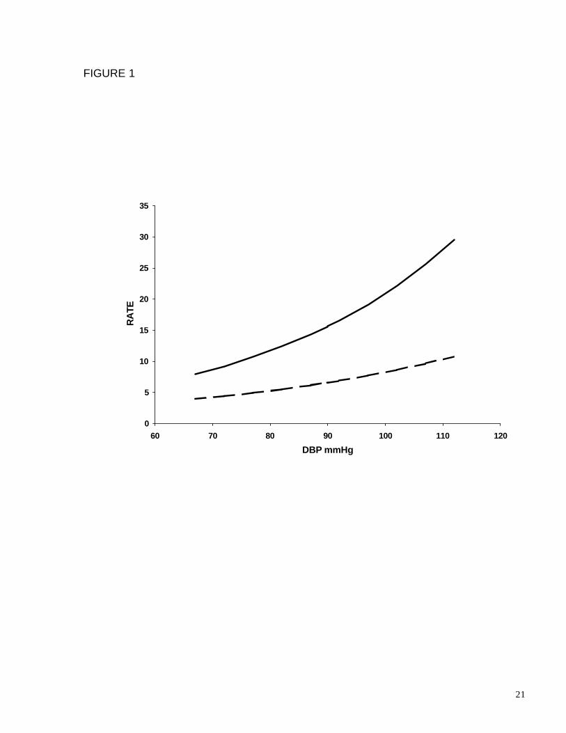
Fig. 1. The Framingham logistically smoothed adjusted death rates per 1000 of

cardiovascular disease incidence (solid line) and mortality (dashed line) for all persons

aged 45-74.

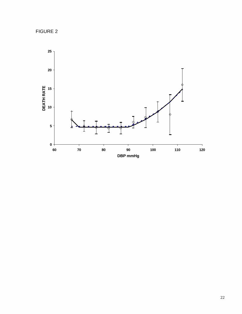
Fig. 2. Adjusted cardiovascular death rates per 1000 as a function of diastolic blood

pressure. Shown are observed death rates (m), 95% confidence intervals for rates

(vertical bars), horizontal 1-spline model (dashed line), horizontal 2-spline model (solid

line).

Fig. 3 Parabolic model and observed rates

Fig. 4. Cardiovascular disease incidence and mortality rates per 1000 Shown are

observed incidence rates (circles), their 95% confidence intervals (vertical bars),

observed death rates (squares). Upper curve: jump model for incidence. Lower curve:

horizontal 2-spline model for mortality.

Table 1 diastolic blood pressure catagories (mm Hg)Category 1 2 3 4 5 6 7 8 9 10Range 020-

069070-074

075-079

080-084

085-089

090-094

095-099

100-104

105-109

110-160

21

FIGURE 1

0

5

10

15

20

25

30

35

60 70 80 90 100 110 120

DBP mmHg

RA

TE

22

FIGURE 2

0

5

10

15

20

25

60 70 80 90 100 110 120

DBP mmHg

DE

ATH

RA

TE

23

FIGURE 3

0

2

4

6

8

10

12

14

16

18

60 70 80 90 100 110 120

DBP mmHg

DE

ATH

RA

TE

24

FIGURE 4

0

5

10

15

20

25

30

35

40

45

50

60 70 80 90 100 110 120

DBP mmHg

RA

TE