dicin papr sri - iza institute of labor economicsftp.iza.org/dp10681.pdf · 2.1. the german public...

Discussion PaPer series

IZA DP No. 10681

Johannes GeyerClara Welteke

Closing Routes to Retirement:How Do People Respond?

mArch 2017

Any opinions expressed in this paper are those of the author(s) and not those of IZA. Research published in this series may include views on policy, but IZA takes no institutional policy positions. The IZA research network is committed to the IZA Guiding Principles of Research Integrity.The IZA Institute of Labor Economics is an independent economic research institute that conducts research in labor economics and offers evidence-based policy advice on labor market issues. Supported by the Deutsche Post Foundation, IZA runs the world’s largest network of economists, whose research aims to provide answers to the global labor market challenges of our time. Our key objective is to build bridges between academic research, policymakers and society.IZA Discussion Papers often represent preliminary work and are circulated to encourage discussion. Citation of such a paper should account for its provisional character. A revised version may be available directly from the author.

Schaumburg-Lippe-Straße 5–953113 Bonn, Germany

Phone: +49-228-3894-0Email: [email protected] www.iza.org

IZA – Institute of Labor Economics

Discussion PaPer series

IZA DP No. 10681

Closing Routes to Retirement:How Do People Respond?

mArch 2017

Johannes GeyerDIW Berlin

Clara WeltekeDIW Berlin and IZA

AbstrAct

mArch 2017IZA DP No. 10681

Closing Routes to Retirement:How Do People Respond?*

We present quasi-experimental evidence on the employment effects of an unprecedented

large increase in the early retirement age (ERA). Raising the ERA has the potential to extend

contribution periods and to reduce the number of pension beneficiaries at the same time,

if employment exits are successfully delayed. However, workers may not be able to work

longer or may choose other social support programs as exit routes from employment. We

study the effects of the ERA increase on employment and potential program substitution

in a regression-discontinuity framework. Germany abolished an important early retirement

program for women born after 1951, effectively raising the ERA for women by three

years. We analyze the effects of this huge increase on employment, unemployment,

disability pensions, and inactivity rates. Our results suggest that the reform increased both

employment and unemployment rates of women age 60 and over. However, we do not

find evidence for active program substitution from employment into alternative social

support programs. Instead employed women remained employed and unemployed women

remained unemployed. The results suggest an increase in inequality within the affected

cohorts.

JEL Classification: J14, J18, J22, J26

Keywords: retirement age, early retirement, regression discontinuity, pension reform, unemployment, labor supply, disability pension

Corresponding author:Clara WeltekeDIW BerlinMohrenstr. 5810117 BerlinGermany

E-mail: [email protected]

* We thank David Blau, Flavia Coda-Moscarola, Gordon Dahl, Peter Haan, Markus Knell, Rafael Lalive, Adam Lederer, Maarten Lindeboom, and Arthur Seibold, and numerous seminar and conference participants for insightful comments and suggestions. We are grateful for the support of Tatjana Mika, Wolfgang Keck, and their colleagues at the Research Data Centre of the German Pension Insurance. ClaraWelteke acknowledges funding from the Research Network of the German Pension Insurance Fund through a doctoral scholarship (Forschungsnetzwerk Alterssicherung - FNA). The views expressed here are solely of the authors. The usual disclaimer applies.

1. Introduction

Population aging presents enormous challenges for public pension systems (OECD, 2015).Most OECD countries answered the challenges posed by increasing old-age dependencyratios by reforming their pension systems. A central aim of these reforms is to extendworking lives alleviating the decline of the working age population (OECD, 2006, 2011).Reforms include increases in the early retirement age (ERA) and increases in the normalretirement age (NRA), i.e. the age at which people can �rst draw full bene�ts withoutactuarial deductions. Germany is characterized by a particularly steep increase in theold-age dependency ratio and low employment rates of older workers. In order to relievepublic �nances by increasing the employment rates of older workers, in a 1999 pensionreform, Germany abolished an important early retirement program for women born after1951. The reform e�ectively raised the ERA for women from age 60 to at least 63. Anincrease in the retirement age has the potential to extend contribution periods and reducethe number of pension bene�ciaries at the same time, if employment exits are successfullydelayed. However, workers may not be able to work longer or may choose other socialsupport programs as exit routes from employment. Large program substitution e�ectscould undermine the potential positive �scal e�ects of the pension reform. Therefore, it isimportant to empirically assess if an increase in the ERA induces increased inactivity orsubstitution into other government programs such as unemployment or disability bene�ts.In this paper, we provide novel empirical evidence on this important research question.

In more detail, we analyze the labor market e�ects of the substantial increase in the earlyretirement age for women. The change in ERA is a large negative wealth shocks for thea�ected cohorts. The reform provides a clean quasi-experimental setting as it induces alarge one-time shift in the ERA. We exploit the unprecedented sharp discontinuity in theERA between cohorts to estimate the causal impact on female employment behavior in aregression discontinuity framework based on high quality administrative data. We knowthe month of birth and compare women born close to the cuto�. Our research designallows us to quantify the causal e�ects of the reform on female employment, take-up of dis-ability pensions, unemployment, and inactivity rates. Furthermore, we focus not only onthe e�ects on levels, but also on employment out�ows into other social security programsas a response to the reform. In contrast to most of the previous literature, we distinguishbetween active program substitution from employment into unemployment, disability pen-sion or inactivity, and passive program substitution, which occurs due to continuance of theformer status because an exit into early retirement is no longer attainable. Furthermore,we examine whether the behavioral reactions are heterogeneous across di�erent groups.Raising the ERA might have undesired distributional e�ects as the ability to work longerand the remaining life expectancy may depend on socio-economic status. In particular,workers with poor health and a weak labor market position might be negatively a�ectedby the reduced retirement options (Staubli, 2011).We contribute to the literature in various ways. Similar to other studies, we exploit

cohort-speci�c variation in incentives to retire (e.g., Mastrobuoni, 2009; Hanel and Riphahn,2012; Cribb et al., 2014; Lalive and Staubli, 2014; Atalay and Barrett, 2015; Manoli andWeber, 2016; Engels et al., 2016). In contrast to previous studies, the reform we analyzeis a large one-time change of pension rules. Usually changes of the retirement age areintroduced in small steps over a longer time horizon, which generally requires stronger as-sumptions to separate the reform e�ect from time trends, other policy reforms, and cohorte�ects. Moreover, many studies focus on changes in the NRA, while only a few analyzethe e�ect of changes in the ERA. Increasing the ERA implies that the choice set of older

2

workers is reduced and that the employment reaction of those who would have chosen toretire depends on the relative attractiveness of the remaining options. There is a large lit-erature that analyzing program substitution e�ects in the context of pension reforms (e.g.,Duggan et al., 2007; Karlström et al., 2008; Li and Maestas, 2008; Coe and Haverstick,2010; Staubli, 2011; Staubli and Zweimüller, 2013; Borghans et al., 2014; Atalay and Bar-rett, 2015; Inderbitzin et al., 2016). However, the existing evidence on the e�ectiveness ofincreasing the ERA and program substitution is mixed. Staubli and Zweimüller (2013) andAtalay and Barrett (2015) �nd that gradual increases in the ERA led to increased programsubstitution in Austria and Australia. In contrast, Manoli and Weber (2016) and Oguzogluet al. (2016) do not �nd evidence for increased active substitution from employment intosocial security programs based on the same reforms.Based on a linear regression-discontinuity design, we �nd that employment rates of

women born in 1952 aged 60 and older increased markedly by 14.4 percentage pointsdue to the reform. Interestingly, employment rates before age 60 remained una�ectedby the reform, even though the reform was long anticipated. Although we �nd evidencefor increased program substitution into unemployment, the increase in the unemploymentrate is not due to active program substitution from employment but rather stems from theinability of unemployed women to retire early after the reform. We do not �nd evidence forincreased unemployment, disability pension, or inactivity entry due to the ERA increase.Based on these results, we draw the following conclusions: First, the reform seems to bean e�ective tool to extend employment of employed women. Second, unemployed womenremain longer in unemployment. Third, we do not �nd evidence for increased take-up ofdisability pensions. Fourth, the results suggests that the reform a�ected certain groupsheterogeneously. We �nd larger positive e�ects on the employment rates of women withlow income or poor health; however, the di�erences are statistically insigni�cant. Wealso �nd larger e�ects on unemployment rates in East Germany than in West Germany,which is consistent with the fact that unemployment rates were higher and early retirementwas more prevalent in the East. Further heterogeneous e�ects of the reform result fromthe persistence of labor market statuses: Unemployed or inactive women remained intheir respective status while employed women continued being employed. A tentativeinterpretation of these results is that the reform increased inequality within the a�ectedcohorts.The paper proceeds as follows: Section 2 brie�y outlines the pension system and the 1999

pension reform. Section 3 derives hypotheses about potential behavioral reactions. Sec-tion 4 describes the administrative data that are used in our analysis. Section 5 describesour empirical strategy and Section 6 presents the results of the empirical analysis, includ-ing a discussion of the heterogeneity of the results across subgroups. Finally, Section 7concludes.

2. Institutional background

In this section, we provide an overview of the German public pension system and itsdi�erent early retirement programs. The 1999 pension reform, which this paper focuseson, is explained in detail. In addition, we discuss interactions of the pension systemwith other social security programs (unemployment and disability pensions) and highlightpotential program substitution patterns.

3

2.1. The German public pension system

The statutory public pension system covers most private and public sector employees.It provides old-age pensions, disability pensions, and survivors bene�ts. The system is�nanced by a pay-as-you-go (PAYG) scheme. The calculation of pension bene�ts is basedon a point system that takes into account the entire earnings history and insurance recordof each individual. A year's contribution at the average earnings of contributors earns onepension point. Moreover, pension points can be acquired during other insurance periods(e.g. unemployment, child raising and while providing informal care). Pensions are roughlyproportional to an individual's average lifetime labor income and feature few redistributiveproperties.1

Depending on the length of the insurance record and other qualifying conditions, theage at which pension bene�ts can be claimed lies between 60 and 65.5 for the cohortsunder study (1951�1952). In addition to the regular pension, which requires 5 years ofcontributions, until 2012 there were four early retirement programs with di�erent qualifyingconditions:

1. Pension for women

2. Invalidity pension

3. Pension after unemployment or old-age part-time work

4. Pension for the long-term insured

The �rst two of these programs allowed retirement starting from 60 years of age, thepension for women and the pension for people with severe disability status (invaliditypension). The NRA, the age at which full bene�ts can be claimed, was di�erent betweenthese programs. The NRA of the pension for women and for the invalidity pension was 65and 63, respectively. Early retirement was associated with actuarial deductions of 0.3%per month before the NRA. That is, retiring through the pension for women at age 60 isassociated with permanent pension deductions of 18%. Deductions amount to 10.8% forpeople eligible for invalidity pensions. The other two early retirement programs allowedretirement starting from age 63. People who are not able to work due to severe healthconditions can retire before the age of 60 through the disability pension program. SeeTable 4 for more details.2

2.2. The 1999 pension reform

The 1999 reform abolished the early retirement program for women in cohorts born after1951. E�ectively, the reform raised the earliest retirement age for most women to at least63. Women born before 1952 could claim the pension for women if they ful�lled certainqualifying conditions. The eligibility criteria were: (i) at least 15 years of pension insurance

1Börsch-Supan and Wilke (2004) provide an extended overview of the German pension system.2Note that the German pension system provides two di�erent types of pensions due to impaired health.The disability pension ("Erwerbsminderungsrente") is similar to disability bene�ts in the US. Eligibilityfor full bene�ts requires that an individual is unable to work more than 3 hours a day for at least sixmonths. Eligibility for partial disability bene�ts require that the individual is unable to work morethan 6 hours a day. Eligibility requires 5 years of contributions. It is the only pension that is availablebefore the age of 60. In addition, there is a second type of old-age pension: the invalidity pension isavailable from age 60 for people with a severe disability status under German law. Invalidity statusrequires a degree of disability of 50% or more and does not require work incapacity. The ERA of thispension has been increased since 2012 (see Table 4).

4

contributions; (ii) at least 10 years of pension insurance contributions after the age of 40.These criteria ensured a minimum labor market attachment of eligible women. Our datashow that about 60% of all women born in 1951 were eligible for the old-age pension forwomen. Take-up was particularly prevalent in East Germany, where most women have astrong labor market attachment and meet the qualifying conditions of this pension type.3

Due to the reform, women born in 1952 lose an important option to exit the labor marketbefore age 63. At age 63, people with a long insurance record can retire with deductions.As explained above, the only remaining pension type before age 63 is the invalidity pension.However, even before the 1999 reform, if women had the the choice between the invaliditypension or the pension for women, the former implied lower deductions. In other words,invalidity pension has always been advantageous compared to the pension for women.Therefore, we do not expect large substitution into the invalidity pension due to the reform.For women born after 1951 who want to exit the labor market before age 63, the remainingoptions are unemployment bene�ts, disability pensions, or inactivity.

2.3. Disability pension, unemployment insurance and inactivity

It is theoretically plausible that some women who would have otherwise claimed old-agepension bene�ts chose another social support program or withdrew from the labor force.In the following, we brie�y describe the design of unemployment insurance and disabil-ity pensions in Germany, focussing on the potential for interdependencies and programsubstitution.Unemployment bene�ts in Germany replace about 60% of previous net earnings and

increase pension entitlements.4 Eligibility and the entitlement period depend on the ageand the previous working history. The maximum entitlement period for unemploymentbene�ts did not change during our observation period. Speci�cally, the maximum entitle-ment period for individuals above the age of 57 was 24 months. Generally, there is a stronginterdependence between unemployment bene�ts and pensions for older individuals. Asdocumented in Grogger and Wunsch (2012), Giesecke and Kind (2013) and Engels et al.(2016), some older individuals use unemployment bene�ts as a bridge into retirement. Inparticular, there is evidence that unemployed individuals exhaust their full entitlementperiod for unemployment bene�ts before entering retirement. The design of the institutionprovides strong incentives for this behavior; unemployment bene�ts are relatively generous,periods in unemployment increase pension entitlements and, lastly, search requirements forunemployed persons close to retirement are very low. Therefore, an increase in the ERA islikely to a�ect the take-up of unemployment bene�ts in two ways: �rst, individuals havean increased incentive to postpone entry into unemployment, if unemployment bene�ts areindeed used as a pathway to retirement. This would lead to a shift in increased unemploy-ment entry from 58 (cohort 1951) to 61 (cohort 1952) years; 24 months before reaching thecohort-speci�c ERA. Second, unemployment rates among 60 to 63 year-old women mayincrease due to program substitution because of the abolishment of the early retirementoption, i.e. because women who want to exit employment between the old and new ERAmust take another path to exit the labor market.The disability pension (Erwerbsminderungsrente) is the only pathway to retirement be-

fore reaching the ERA. Eligibility requires the long-term (at least six months) inability to

3The pension due to unemployment or after old-age part-time work was abolished at the same time asthe pension for women. However, this does not a�ect our analysis as the ERA for this pension typewas already 63.

4People receiving unemployment bene�ts acquire pension entitlements as if they earned 80% of theirprevious gross earnings.

5

perform an activity under normal labor market conditions for at least six hours (partialdisability pension) or at least three hours (full disability pension) per day. The pensionis calculated based on the previous insurance biography and amounts to the pension thatwould be paid had the individual continued to work until she turned 60. When reachingthe statutory retirement age, the disability pension is converted into an old-age pensionusually of the same level. In Germany, health-related eligibility criteria for disability pen-sions are relatively strict, especially sine a 2001 reform. About 40% of all applications arerejected. Therefore, using disability pensions as a pathway to a regular old-age pension isdi�cult and not typically an attractive option. Moreover, since 2001, actuarial deductionsalso apply to this type of pension. The pension is permanently reduced by 0.3% per monthif retiring before the NRA. In 2012, the NRA of disability pensions was increased from 63to 65, with deductions capped at a maximum of 10.8%. Virtually all of these pensions arereduced by maximum deductions since most people claim this pension before turning 60(Deutsche Rentenversicherung, 2015, p.83).Individuals who are neither eligible for disability pension nor unemployment bene�ts

may choose inactivity, i.e. exit the labor force without bene�t receipt. This is particularlyrelevant for women, who often are not the primary earner in their households.

3. Expected reform e�ects

The reform of 1999 is expected to have several e�ects on employment outcomes. We expectwomen born after 1951 to extend employment and to delay retirement entry compared towomen una�ected by the reform. Since the reform did not just increase the penalty forearly retirement but abolished the option altogether, we expect large e�ects on employmentrates of wome aged 60 to 63. However, not all women are able or willing to work untilreaching the new ERA. Therefore, we expect increased program substitution, which is theresponse to similar reforms in other countries (see Staubli and Zweimüller, 2013; Atalayand Barrett, 2015).Following Oguzoglu et al. (2016), we distinguish between two di�erent kinds of e�ects:

active and passive (mechanic) program substitution. Women who do not have an option toretire at 60, even though they would have retired in the absence of the 1999 reform, mustdivert into another employment status or continue their previous status. The continuationin a social security program due to the lack of a retirement option can lead to a passive in-crease in e.g. unemployment and inactivity rates. In contrast, active program substitutionrefers to �ows from employment into other social security programs as a response to theelimination of the retirement option. In order to distinguish between passive and activeprogram substitution, we analyze employment out�ows into other social security programsaround age 60. There are mainly the two aforementioned social security programs thatare relevant in this context: unemployment insurance and disability pensions (explainedin detail in Section 2.3). As a third option, we consider potential increases in inactivityrates.There are several reasons why we expect the 1999 reform to e�ect employment outcomes

before the former ERA of 60. First, women born after 1951 who have a preference for earlyretirement around the age of 60, may choose alternative pathways to exit employment,perhaps even before their 60th birthday, instead of delaying until they reach the ERA. TheERA can serve as a reference age for retirement decisions (see Seibold, 2016), which leadsto the bunching of retirement entries at the ERA, and a reduced number of exits amongindividuals approaching the reference age. Consequently, an ERA increase may lead to anincrease in employment exits of women approaching age 60. We refer to this e�ect as the

6

reversed reference-age e�ect.Second, women may bridge the last one or two years prior to reaching the ERA with

unemployment. As explained in the previous section, German workers have an incentiveto exit employment two years before reaching the ERA through unemployment bene�ts,which are paid for up to 24 months to older workers. An increase in the ERA leads to a shiftin the bridge period. If women adjust their employment behavior and delay their (bridgeinto) retirement, we expect a negative e�ect on unemployment and disability pension ratesfor women approaching age 60, in particular among 58 and 59 year-old women. Insteadwe would expect women born after 1951 to enter unemployment at 61 or 62 years of agemore often.Third, the ERA increase was announced in 1999, while it only a�ected women turning 60

in 2012. Consequently, the ERA increase was known when the �rst a�ected cohort was 47years old. It is not obvious a priori how younger women will adjust their labor supply in aresponse to the increased ERA. The reform can be interpreted as a strong negative wealthshock as it reduces the length of time that women receive pension bene�ts. Theoretically,this should have a positive e�ect on labor supply. If these women were forward looking,they might have adjusted labor supply as soon as the legislation was passed.5

4. Data

We use high-quality administrative data from public pension insurance accounts (VSKT:Versicherungskontenstichprobe).6 VSKT is a strati�ed random sample of all pension in-surance accounts of people aged 30 to 67. The VSKT is representative of the Germanpopulation of public pension insurance accounts, if the appropriate sampling weights areused. Since the data are process-produced, recall errors due to memory gaps and wrongtemporal assignment are avoided, while panel mortality is negligible (Fachinger and Him-melreicher, 2006). The data include the month of birth of each individual which allows tocompare women born close to the cuto�. Furthermore, individual employment behaviorand retirement entry is reported with monthly accuracy. A drawback is that socio-economicvariables are only recorded to the extent that they are relevant for the calculation of pen-sion bene�ts. Consequently, information on education is missing in about half of the cases.Information about occupations is only available for the last occupation at the time of datacollection, which may not be representative of entire employment histories. Furthermore,it is not possible to link spouses and other household members within the data.7

For our analysis we use the VSKT of 2014, the latest available wave at the time of

5We do not expect strong behavioral reactions to the changed incentives of the qualifying conditions.The eligibility criteria of the pension for women (namely after 15 years of pension contributions) areno longer relevant for cohorts born after 1951. However, early retirement at 63 requires the completionof a contribution period of 35 years, including child raising periods. It is not clear how the changein eligibility criteria for early retirement a�ects the labor supply of women between 47 and 59. Forexample, a woman in the 1951 cohort with 14 years of contributions has a strong incentive to work atleast one additional year to qualify for early retirement. The incentive to accumulate 35 contributionyears is higher for cohorts born after 1951. The data show a large overlap between women who ful�llthe criteria of the pension for women and those who ful�ll the eligibility criteria for early retirementfor the long-term insured. A graphic representation of the distribution of pension contribution years isin Appendix C.3. As documented in Seibold (2016) bunching around these thresholds is present, butit is very small and In fact, the vast majority of women who quali�ed for the pension for women werealso eligible for long-term insured pension.

6We use the full VSKT, which is roughly four times as large as the scienti�c-use �le SUFVSKT and canonly be accessed on-site.

7A detailed description of the data can be found in Himmelreicher and Stegmann (2008).

7

analysis. We restrict the sample to women born 12 months before and after the cuto�(cohorts 1951 and 1952). Furthermore, we exclude all women who paid contributions toa special miners' pension scheme (Knappschaftliche Versicherung) for at least one month,which applies to about 10% of all women. Another group excluded from our sample (about6% of all women) consists of all women receiving an old-age invalidity pension at some pointin their life.8 After dropping these groups, we are left with 7,365 women.9

The 1999 pension reform increases the ERA only for women who were eligible for thepension for women. Women who did not meet the qualifying conditions, are mot likelyto be eligible to any early retirement program. In our analysis, we therefore focus onwomen who ful�ll the eligibility criteria for the pension for women.10 Those criteria arethe accumulation of at least 15 years of pension contributions, with 10 years after turning40. About 60% of the women in our sample ful�ll these eligibility criteria. Due to thetraditionally stronger labor market attachment of women in East Germany, the share ofeligible women amounts to more than 80% for East German women. Our �nal sampleconsists of 3,771 women who ful�ll the eligibility criteria of the pension for women. About30% of the eligible women in the sample (cohort 1951) retire early through the early pensionfor women before their 62nd birthday.The main variables of interest in this analysis are whether or not an individual is em-

ployed, unemployed, inactive, or receiving a disability pension at any given age in months.11

A woman counts as employed if she had a job which was subject to social security contri-butions or if she was marginally employed.12 The best approximation of inactivity is theresidual category, which comprises all statuses that are not employment, unemployment,or pension receipt. The residual category includes periods of education or training, insuredself-employment, non-commercial care for children or elderly family members, illness, andunknown status (missing value). By far the largest group within the residual categoryconsists of women with missing employment status. We refer to the residual category asinactivity in the remainder of this paper. These women coule, in principle, be working asuninsured self-employed or as civil servants since these statuses are also recorded as miss-ing values. However, this is very unlikely in the sample we select: women older than 58who qualify for the pension for women. That is, women who paid 10 years social securitycontributions after their 40th birthday.13

In order to analyze heterogeneous e�ects by income and health, we use information onaverage pension points and periods of sick-pay to approximate income groups and health

8As argued in Section 2.2, if women had the choice to either retire through the pension for women orthe invalidity pension, the invalidity pension is always superior to the pension for women since it isassociated with lower pension deductions. Therefore, we assume that the 1999 pension reform did nota�ect this group.

9We account for regional di�erences in the empirical analysis since the employment behavior of womenin East and West Germany di�ers markedly. About 17% of the sample collected most of their pensioncontribution points in East Germany. The assignment of a region to individual employment histories isstraightforward because very few women in the relevant cohorts earned non-negligible pension pointsin both East and West Germany.

10We discuss potential bias due to sample selection in Appendix C.3. Furthermore, we include an analysisusing a sample of all women regardless of pension eligibility in Appendix C.4.

11We de�ne disability pension periods as months with pension receipt before reaching the ERA; and byusing the pension-type information for current pension spells. If a disability pension is converted intoan old-age pension, the months of old-age pension receipt are re-coded as disability pension periods.

12Marginal employment (geringfügige Beschäftigung) is de�ned as a tax-free employment-relationship withearnings under a certain threshold (until 2013 up to 400e/month, since 2013 450e/month).

13Note that inactivity is used here to describe the status of out of the labor force and of the social securitysystem. Therefore, it includes e.g. housework or care for a family member, which should not bemisinterpreted as leisure or idleness.

8

status. A women is de�ned to belong to the low income group if she is in the lowestthird of the distribution of average pension points over all full contribution periods.14

The low income group is de�ned by having accumulated on average less than 0.52 annualpension points. That is equivalent to 52% of average earnings or 18,126 euro for a WestGerman woman in 2014.15 Note that we use individual pension points, which are basedon individual earnings. We approximated poor health using periods of sick-pay, which areonly recorded if the sick leave exceeds six weeks or entails hospitalization for employedindividuals. A person is de�ned as having a poor health status if she has at least onesick-pay spell between age 45 and 55, which holds true for about 26% of the sample ofeligible women.16

4.1. Descriptive evidence

The distribution of employment status by age group is displayed in Figure 1 for the 1951and 1952 cohorts. The employment rates of 58 and 59 year-old women are relatively highdue to the sample restriction to women eligible for the pension for women. It shows thata large fraction (26%) of women born in 1951 receive an old-age pension from their 60th

birthday onward. This fraction disappears if we look at the 1952 cohort, due to the ERAincrease. Employment, unemployment, and inactivity rates increased for 60 and 61 year-old women born in 1952 (treatment group) compared to women born in 1951 (controlgroup). In particular, the employment rate amounts to 70% in the cohort 1952, where itis 54% in the 1951 cohort.

Figure 1: Employment status by age group and cohort, sample of eligible women

Cohort 1951 Cohort 1952

73%

54%

26%

0%

10%

20%

30%

40%

50%

60%

70%

80%

90%

100%

58-59 60-61

75% 70%

0%

10%

20%

30%

40%

50%

60%

70%

80%

90%

100%

58-59 60-61

Residual

Old-age pension

Disability pension

Unemployment

Employment

Source: VSKT 2014, own calculations

A closer look at the fractions of women in di�erent employment status across age revealsthat women born in 1951 exhibit a large drop in employment rates when reaching age 60,

14We used the pension points (avegpt) earned over full contribution periods only (byvl). Points earned inthe East and West are treated equally; however, percentiles are constructed separately for East andWest German women, using all women (not just eligible women).

1518,126 = 0.52 x 34,857, where 34,857 was the average gross earnings of all insured individuals in WestGermany in 2014.

16Employed women are more likely to receive sick-pay, therefore, the sub-sample of women with poorhealth is likely to be employed between 45 and 55.

9

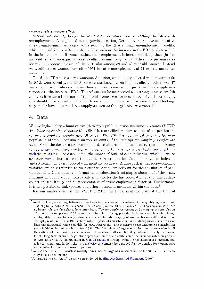
while this discontinuity is not observed for the 1952 cohort (Figure 3a). Not surprisingly,the fraction of women receiving a pension (including disability pensions) increases sharplyat the ERA for the 1951 cohort (Figure 3b). There is no visible di�erence in employmentand retirement rates between cohorts before reaching age 60.

Figure 2: Employment and pension recipient rates by age and cohort

(a) Employment rate (b) Pension recipients

Notes: Employment includes marginal employment.Source: VSKT 2014, own calculations

Figure 5a and Figure 5b show that the fraction of women in marginal employment andthe unemployment rate are slightly higher for the 1952 cohort for all ages between 55and 60. At age 60 however, we observe a drop in marginal employment and unemploymentrates of the 1951 cohort. From age 60 to 62, the 1952 cohort is more likely to be marginallyemployed and unemployed. It can be seen in Figure 5d that the fraction of inactive womenalso drops sharply when reaching age 60, indicating that a large share of women whowere previously inactive start receiving the pension for women. The fraction of womenreceiving a disability pension increases continuously with age for both cohorts (Figure 5c).It can also be observed that women born in 1951 are slightly more likely to receive adisability pension (Figure 5c), in particular between 57 and 61 years of age. Note thatdi�erences between cohorts and �uctuations over time can be due to e.g. time trends ormacroeconomic shocks. However, our empirical identi�cation strategy is not threatened aslong as di�erences between cohorts are continuous over the month of birth (see Section 5for a detailed description of our empirical strategy.)While the sharp decrease in the proportion of women born in 1951 in several employment

categories suggest an out�ow into early retirement, an analysis of employment out�owsis needed to gain further insights on employment exit behavior and potential programsubstitution e�ects. In particular, we cannot infer from Figure 4 whether the reform ledto increased in�ow into unemployment, disability pension, or inactivity from employment.Employment out�ows are displayed in Figure 7a to Figure 7d. The employment exit

hazard rate is de�ned as the fraction of women exiting employment at age t, conditionalon survival in employment (excluding marginal employment) up to age t, out of all womenwho were employed for at least six months when reaching age 58. Unemployment, disabilitypension, and inactivity entry rates are de�ned as the probabilities to enter the respectivecategory conditional on having survived until t, and employment (including marginal em-ployment) for at least six months at their 58th birthday. Note that we do not condition onemployment between age 58 and the �rst unemployment, disability pension or inactivityentry event. We only consider the �rst exit or entry, i.e. reentering the sample is not

10

Figure 4: Employment status by age and cohort

(a) Marginal employment (b) Unemployment

(c) Disability pension (d) Inactivity

Notes: The inactivity category combines all status except (marginal) employment, unemployment, old-agepension, or disability pension receipt.Source: VSKT 2014, own calculations

possible. It can be seen in Figure 7a that the employment exit hazard peaks at age 60(one month after the 60th birthday) and, to a lesser extent, at age 61 for the 1951 cohort,while the hazard remains �at for the 1952 cohort.If women in our sample used 24 months of unemployment bene�ts receipt as a bridge to

retirement, we would expect a peak in unemployment entry at age 58 for the 1951 cohort,and at age 61 for the 1952 cohort � or at least higher entry rates in the two years beforereaching the ERA. With respect to active program substitution due to the pension reform,we expect increased entry into unemployment and disability for the 1952 cohort at aroundage 60. However, neither are observed in Figure 7b. Therefore, it would be surprising if wediscovered a large shift in unemployment entry or increased program substitution in theregression discontinuity analysis. The entry rates into disability pension and inactivity donot exhibit notable peaks, nor are there observable di�erences between cohorts (Figure 7cand Figure 7d).These descriptive results suggest that there is not increased substitution from employ-

ment into unemployment, disability pension programs or inactivity due to the ERA in-crease. However, the hazard rates displayed here are descriptive only. At each age, thepopulation that survives in employment is selective, based on previous hazard rates. There-fore, one cannot interpret the di�erences in hazard rates between cohorts in a causal sense.A more rigorous empirical analysis, described in the following section, is necessary to assess

11

Figure 6: Employment exit and entry rates into other status by age and cohort

(a) Employment exit (b) Unemployment entry

(c) Disability pension entry (d) Inactivity entry

Source: VSKT 2014, own calculations

whether the ERA increase led to extended employment and substitution into unemploy-ment and disability pension programs or inactivity around the former ERA.

5. Empirical strategy

The empirical identi�cation of the e�ect of pension eligibility rules on labor supply andretirement behavior is challenging: Employment histories and unobserved preferences forwork and leisure a�ect both labor supply in old-age as well as eligibility for early retirement.One way to circumvent this endogeneity problem is to exploit exogenous variation in thepension system over time or cohorts due to policy changes. Our empirical strategy makesuse of the 1999 pension reform, which eliminates the option to retire at age 60 for womenborn in 1952 and thereafter.In the �rst part of our empirical analysis, we employ a linear regression discontinuity

research design to estimate the causal e�ect of an increase in the ERA on employmentrates, unemployment rates, the fraction of older women receiving a disability pension, andthe fraction of inactive women. The regression discontinuity design solves the endogeneityproblem by exploiting variation in the ERA by month of birth. It is valid, if we innocuouslyassume that labor supply at a given age would be continuous over the month of birth inabsence of the 1999 reform.The research design is implemented by the following empirical model:

12

yit = α+ βDi + γ0f(zi − c) + γ1Dif(zi − c) +X ′itδ + εit (1)

Where the indicatorDi = 1, if the individual was born after January 1952. The subscriptt refers to age in months and ranges from 721 to 744 (age 60 to 62 in monthly steps) inthe baseline speci�cation. The month of birth zi enters the empirical model in di�erenceto the reform cuto� c, which is January 1952. In our baseline speci�cations, we includea linear trend in the running variable, f(zi − c) = zi − c. The speci�cation allows fordi�erent slopes before and after the cuto�. All regressions include calendar month �xede�ects, and dummies for three income groups, children, and region, summarized in Xit.However, droppingXit does not change the point estimates (see Appendix C.5 for regressionresults without covariates). Regression discontinuity analyses are naturally prone to modelmisspeci�cation. A non-linearity in outcomes may falsely be interpreted as a discontinuityif it is unaccounted for. Therefore, we report linear regression results both with linear andquadratic trends in the running variable (RDD results with quadratic trends are displayedin Table 14 in Appendix C.6). Furthermore, we support our analysis by graphical analysesof local linear regression plots.Employment status data is recorded for each individual at every age in months t. There-

fore, we need to specify a time-window for the outcome variables of interest. In our baselinespeci�cation, we pool all observations from the month after the 58th birthday to the 60th

birthday (age 58-59 ), and all observations from the month after the 60th birthday to the62nd birthday (age 60-61 ).17 In order to account for correlation between observations forthe same individual or individuals born in the same month, we cluster standard errorsby month of birth. The baseline speci�cation allows us to estimate treatment e�ects forfour outcome variables for two age groups before and after age 60. However, it may be ofinterest to estimate a more �exible model that allows for heterogeneous e�ects for everyage in months t. Consequently, we analyze the reform e�ects for every age in months sep-arately by including age-treatment interactions into our empirical model. The inclusion ofage-dummies and interactions with the treatment variable Di = 1, allows us to interpretthe coe�cient of the interaction term as the reform e�ect on a speci�c age group (seeSection 6.2).In the second part of the empirical analysis, we focus on active program substitution

due to the ERA reform (similar to Manoli and Weber (2016) or Oguzoglu et al. (2016)).In more detail, using a sub-sample of women who were employed on their 58th birthday,we estimate out�ows from employment, and in�ows into unemployment bene�ts, disabilitypension, and inactivity (see Section 6.4). If we look at the e�ects on the shares in di�erentemployment categories only (as in Equation 1), we cannot distinguish between passive andactive program substitution. In contrast, an analysis of employment out�ows allows us toanswer the question whether women increasingly used alternative social security programsto exit employment in response to the abolishment of the early retirement option.18 Wecircumvented the dynamic selection problem by conditioning on employment at a �xed agein months. Formally, we estimate the same regression discontinuity model as described inEquation 1; however, the outcome of interest is the probability to exit employment (intounemployment or disability pension programs) within the following 2-4 years, conditional

17In order to have equal treatment and control groups, we do not include observations after their 62nd

birthday, which are only available for the older women in the sample.18A drawback of survival data is that if one compares the hazard rates of two groups over time, the group

composition changes if one group has a higher exit probability. This is called the dynamic selectionproblem. Consequently, we cannot estimate treatment e�ects by comparing the di�erence in hazardrates between cohorts over age in months.

13

on employment for at least six months at the 58th birthday. Conditioning on employmentat certain age is problematic if it is itself an outcome that is potentially a�ected by thereform. However, we can show that there is no discontinuity in the employment rate atthe sample entry age of 58 (Figure 12 in Section 6.4). Consequently, we argue that treat-ment e�ects on �ow variables can consistently be estimated using the linear RD approachdescribed above.

5.1. Threats to identi�cation

The RD design is only valid if women cannot manipulate the treatment assignment variable(Lee and Lemieux, 2010), which is the month of birth in our research design. Evidently,it is impossible that women or their parents manipulated the date of birth in anticipationof the policy change, as the reform was introduced long after the cohorts in question wereborn. Furthermore, we are not aware of any discontinuous changes in the incentive to givebirth in December 1951 as opposed to January 1952.19

One of the most important assumptions of our analysis is that any discontinuities in theoutcome variables at the cuto� are solely due to the 1999 pension reform. In particular, weneed to assume that the di�erences between the cohorts in question are not caused by otherpolicy changes. Two other pension policy changes also became e�ective for individuals bornafter January 1st, 1952. First, the old-age pension for the unemployed was abolished forall individuals born after 1951 as part of the 1999 pension reform. However, the ERAfor this pension was already at 63. Therefore, this change did not a�ect women at age60. Second, the ERA of the invalidity pension program was increased from 60 to 63 inmonthly steps starting with individuals born in January 1952. We exclude all women whoreceived an invalidity pension because the ERA for the invalidity pension was also changedfor the same cohorts as for the pension for women. It can be assumed that women eligiblefor either pension will choose the invalidity pension due to the signi�cantly more generouspension bene�ts.Even in the absence of other reform changes, women born in 1952 may still be di�erent

from women born earlier due to time trends in employment outcomes. Employment ratesof women have been increasing over the past decades for every age. Including linear orquadratic trends in birth-dates should resolve this issue in an RD research design, as longas we can assume that women who were born close to the cuto� are not di�erent from eachother. This is tested by checking for discontinuities in covariates, using the same regressiondiscontinuity framework. Results from the test for covariate discontinuities are displayedin Table 7 in Appendix C.1. We do not �nd signi�cant discontinuities in covariates thatare not inherently in�uenced by the 1999 reform. Furthermore, we perform a di�erence-in-discontinuities analysis in order to test whether our results are caused by a turn of the

year e�ect. Reassuringly, the results of the di�erence-in-discontinuity analysis, displayed inTable 8 and Table 9 in Appendix C.2, do not di�er signi�cantly from our baseline results.A possible concern arises due to the selection of the sample by the eligibility criteria

of the pension for women. Speci�cally, women born in 1951 may select into the sampleby extending their pension contribution period in order to be eligible for early retirement.In contrast, women born in 1952 do not have the same incentives to ful�ll the eligibilitycriteria. We discuss the problem of sample selectivity in Appendix C.3. We show that thepotential bias due to selection is negligible because there was no change in the fraction ful-�lling early retirement eligibility criteria due to the reform. We repeat the analysis withoutsample restrictions using all women born 1951 and 1952 regardless of pension eligibility

19It can be shown that the number of observations is relatively stable across all months of birth.

14

criteria. We �nd that the pattern of the reform e�ects is very similar when including thenon-eligible women yet e�ects are at a lower level. The results are in Appendix C.4.

6. Results

6.1. Baseline results

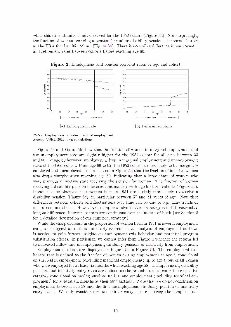
The results of the linear regression discontinuity analysis are displayed in Table 1. Fig-ure 9a to 9d visualize the results using local linear regression on both sides of the cuto�,a triangular kernel, and a bandwidth of 12 months.The increase in the ERA had an average positive e�ect of 14.4 percentage points on the

employment rate of 60 and 61 year-old women (see Column 1, Table 1). The coe�cientscan be interpreted as the average percentage point change in employment rates of allwomen in this age group due to the pension reform. Compared to the pre-reform mean therelative increase amounts to more than 26%. The fraction of women receiving a pensionmechanically dropped by 25 percentage points to zero (Column 5). About 58% of thosewomen, who would have retired if they had the option, continue to work due to the reform.The remaining women split equally in unemployment and inactivity.In addition to the e�ects on employment rates, we estimate the e�ects of the ERA in-

crease on the unemployment rate (Column 2), the fraction of women receiving a disabilitypension (Column 3), and the fraction of inactive women (Column 4). The unemploy-ment rate and the fraction of women in the inactive category increased signi�cantly by5.2 percentage points on average due to the ERA increase. The positive e�ect on theunemployment rate can be due to either a passive increase in the unemployment rate oran active program substitution from employment into unemployment. The zero e�ect ondisability pension participation rates suggests that there is not program substitution intothe disability pension program. i.e. the disability pension program is not used as analternative pathway to enter retirement.Our results suggest that the linear trend in month of birth does not a�ect the outcome

on either side of the cuto�. Whether or not a woman has children does not a�ect theoutcome signi�cantly. Women in West Germany are more likely to be employed, to receivea disability pension, or to be inactive, while East German women are more likely to beunemployed. Note that the results do not change if we drop all covariates (see Table 12Appendix C.5). Including a quadratic function of month of birth does not alter the resultconsiderably (see Table 14 in Appendix C.6).

15

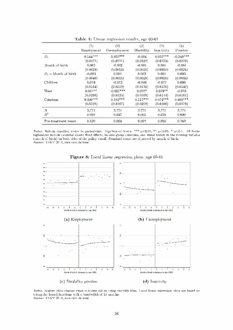
Table 1: Linear regression results, age 60-61

(1) (2) (3) (4) (5)Employment Unemployment Disability Inactivity Pension

Di 0.144*** 0.052*** -0.004 0.052*** -0.249***(0.0271) (0.0111) (0.0232) (0.0123) (0.0270)

Month of birth 0.002 -0.002 -0.001 0.001 -0.001(0.0029) (0.0013) (0.0020) (0.0010) (0.0026)

Di ×Month of birth -0.003 0.001 0.003 0.001 0.003(0.0040) (0.0016) (0.0029) (0.0018) (0.0033)

Children 0.010 -0.013 -0.006 -0.017 0.000(0.0164) (0.0119) (0.0132) (0.0128) (0.0142)

West 0.051** -0.067*** 0.022* 0.029** -0.018(0.0206) (0.0125) (0.0109) (0.0114) (0.0161)

Constant 0.380*** 0.181*** 0.117*** 0.074*** 0.409***(0.0328) (0.0167) (0.0278) (0.0206) (0.0379)

N 3,771 3,771 3,771 3,771 3,771R2 0.058 0.037 0.005 0.018 0.090

Pre-treatment mean 0.538 0.068 0.092 0.050 0.262

Notes: Robust standard errors in parentheses. Signi�cance levels: *** p<0.01, ** p<0.05, * p<0.1. All linearregressions include calendar month �xed e�ects, income group dummies, and linear trends in the running variable(month of birth) on both sides of the policy cuto�. Standard errors are clustered by month of birth.Source: VSKT 2014, own calculations

Figure 8: Local linear regression plots, age 60-61

(a) Employment (b) Unemployment


Notes: Scatter plots display mean outcome values using monthly bins. Local linear regression plots are based ontriangular kernel functions with a bandwidth of 12 months.Source: VSKT 2014, own calculations

16

6.2. E�ects across the age pro�le

In order to shed more light on the e�ects of an ERA increase on employment outcomesat di�erent ages, we interact the entire age pro�le (in months) with the right hand sideof our regression equation. Thereby, we allow for heterogeneous treatment e�ects by agein months. The resulting coe�cients by age in months are displayed in Figure 11a toFigure 11d. The results suggest the e�ect on employment rates of 60 to 62 year old womenis positive and increasing with age. The gradual increase after age 60 is due to pre-reformpension entry past age 60. As expected, we can observe a positive e�ect on unemploymentand inactivity rates from age 60 onward due to the elimination of the option to retireearly. Our results suggest that the fraction of women receiving a disability pension did notincrease for any age-group.There are several reasons why we expect the ERA increase to have an e�ect on employ-

ment outcomes before the former ERA of 60 (see Section 3). The results of our baselinelinear regression analysis on employment outcomes of 58 and 59 year-old women are dis-played in Table 5 in Appendix B. As described in Section 3, we expect a decrease in theunemployment rate of 58 to 60 year-old women and an increase in unemployment ratesfor 61 year-old women, if women are bridging the last 24 months before retirement entrywith unemployment bene�ts. However, we do not �nd evidence for bridging behavior (Fig-ure 11b). The pooled regression for women aged 58 and 59, displayed in Table 5, con�rmsthat there is no signi�cant increase in unemployment rates for this age group. However,we can see in Figure 11b that there is a small positive e�ect on the unemployment rateof some age-groups approaching age 60, which is consistent with a reversed reference agee�ect.Furthermore, we do not �nd evidence for cohort di�erences in employment and inactivity

rates before age 60, as shown in Figures 11a, and Figure 11d. We conclude that, eventhough the ERA increase was long anticipated, there was little or no adjustment in laborsupply in anticipation of the ERA increase.

17

Figure 10: Coe�cients of ERA increase by age in months



Notes: The coe�cients of the treatment dummy interacted with the age pro�le are estimated using a linear regressionmodel including age �xed e�ects, linear trends in month of birth and the interaction with age in months, calendarmonth �xed e�ects, income groups, and a dummy for West Germany. Con�dence intervals of clustered standarderrors are displayed using error bars.Source: VSKT 2014, own calculations

6.3. E�ect heterogeneity by subgroups

In order to understand the impact of the ERA increase, it is necessary to learn more aboutthe group a�ected by the reform. A comparison of women who retire early with thosewho retire with 62 or later, displayed in Table 16 in Appendix D, provides insights on thecharacteristics of the group a�ected by the pension reform. Women who retire early havefewer pension points on average, i.e. lower average earnings. The sum of pension points,contribution points after age 40, and the total contribution period are also lower for earlyretirees, which is not surprising due to the shorter working lifetime. Furthermore, womenwho retire early are more likely to have poor health. Women who retire late are more likelyto be employed and less likely to be unemployed when they reach age 60.If women who make use of the early retirement option di�er from those working longer,

we expect the abolishment of the early pension for women to have heterogeneous e�ectson di�erent subgroups. Therefore, we split our sample into several sub-samples to evaluatewhether the reform had heterogeneous e�ects. In particular, we distinguish between Eastand West Germany.20 Furthermore, we distinguish women with low income, poor health

20A woman is de�ned as West German if she collected the majority of her pension contribution points in

18

and women with and without children.21

The results for the analysis of di�erent subgroups are displayed in Table 2 (and Table 6in Appendix B for 58-59 year-old women). Women in East Germany are much morelikely to be eligible for the woman's pension. Consequently, we �nd larger, although notsigni�cantly, employment e�ects for East Germany than for West Germany. While thereform e�ect on unemployment rates of 60 and 61 year-old women is negligible in WestGermany, there is a large positive e�ect of about 15 percentage points on the unemploymentrate of women in East Germany. This is likely to be due to larger overall unemploymentrates in the East.

Table 2: Subgroup analysis - linear regression results, age 60-61

(1) (2) (3) (4)Employment Unemployment Disability pension Inactivity N

Baseline 0.144*** 0.052*** -0.004 0.052*** 3771(0.0271) (0.0111) (0.0232) (0.0123)

West Germany 0.124*** 0.015 0.007 0.062*** 2727(0.0430) (0.0147) (0.0283) (0.0197)

East Germany 0.184** 0.149*** -0.028 0.026 1044(0.0675) (0.0375) (0.0381) (0.0212)

Low income 0.178*** 0.028 -0.032 0.067** 1046(0.0443) (0.0251) (0.0304) (0.0310)

Poor health 0.159*** 0.045** -0.008 0.051* 988(0.0512) (0.0206) (0.0669) (0.0252)

Children 0.144*** 0.053*** 0.005 0.042** 3198(0.0274) (0.0140) (0.0245) (0.0156)

No children 0.152*** 0.039 -0.075 0.099*** 573(0.0446) (0.0308) (0.0472) (0.0291)

Notes: Robust standard errors in parentheses. Signi�cance levels: *** p<0.01, ** p<0.05, * p<0.1. All linearregressions include calendar month �xed e�ects, income group dummies, and linear trends in the running variable(month of birth) on both sides of the policy cuto�. Standard errors are clustered by month of birth.Source: VSKT2014, own calculations

We expect women to su�er disproportionately by an ERA increase, if they have a strongerpreference to retire early than the average population. Retirement incentives with respectto income groups are not unambiguous due to income and substitution e�ects. We �ndslightly larger e�ects on employment rates for the sub-group of women with low averageearnings. We do not �nd a signi�cant increase in unemployment for this group.Women with poor health can be expected to have strong preferences for early retirement

and inelastic labor supply at high ages. Consequently, we expect women with poor healthto shirk into alternative employment-exit paths when the ERA is increased. In particular,we expect larger unemployment rates and an increase in disability pension participationrates. Our results show that the disability pension rates did not increase for any subgroupas a response to the ERA reform. Among women without children, the e�ect on inactivityrates is larger than for the whole sample including women with children.Overall, we conclude that the ERA increase a�ected certain groups heterogeneously.

Women in East Germany are more a�ected than women in the West. In particular, un-

West Germany.21Low income is de�ned by the lowest third of the distribution of pension points collected in full contribu-

tion periods. Poor health is de�ned as having at least one sick-pay spell from age 45 to age 55. Notethat women who received sick pay are more likely to be employed or unemployed than inactive. Dueto data limitations, we cannot divide the sample into married and unmarried women, even though thiswould be another sub-group analysis of interest.

19

employment rates of 60 to 62 year-old women increase more in East than West Germany.Furthermore, we �nd suggestive evidence for slightly higher employment e�ects for 60 and61 year-old women with low income, poor health and women without children.

6.4. Employment out�ows and program substitution

The results described in the previous sections suggest that the ERA increase led to in-creased program substitution into unemployment. Furthermore, we �nd evidence for in-creased inactivity of 60 to 62 year-old women as a response to the reform. This could becaused by passive (women remain in their respective labor market status) or active substi-tution from employment into unemployment or inactivity because women are not willingor able to work until the new ERA. In order to distinguish between passive and activeprogram substitution, we estimate the e�ect of the ERA increase on the probability to exitemployment (and enter unemployment, disability pension program, or residual category)in a speci�c age window, conditional on employment for at least 6 months at the start ofthis window. In particular, we condition on employment for at least 6 months at the 58th

birthday and estimate the e�ects on the probability to exit employment in the followingtwo and four years. For identi�cation of the treatment e�ect, we have to assume thatemployment rates at age 58 are una�ected by the reform. A test of discontinuity in theemployment rate at the 58th birthday is displayed in Figure 12. There is no statisticallysigni�cant discontinuity in the employment rate at the cuto�.22

Figure 12: Test for discontinuity in employment rate at 58th birthday

Notes: The scatter plot displays mean outcome values using monthly bins. The local linear regression plot is basedon triangular kernel functions with a bandwidth of 12 months.Source: VSKT2014, own calculations

The results for the employment out�ow analysis are displayed in Table 3, where thecoe�cients in the odd columns can be interpreted as the reform e�ect on the probability toexit/enter the respective category between the 58th and the 60th birthday. The coe�cientsin the even columns correspond to the e�ects on the probability to exit/enter the respectivecategories in the four years between the 58th and the 62nd birthday. We �nd a large negativee�ect of 21 percentage points on the probability to exit employment between age 58 and62, which is solely due to decreased exit rates between 60 and 62. Furthermore, we �ndsmall positive e�ects on unemployment, disability pension and inactivity entry rates of 58and 59 year-old women who were employed at their 58th birthday. This could be explained

22This is supported by a regression analysis that is not reported here.

20

by a small reversed reference age e�ect, i.e. by a lack of entries in these categories in the1951 cohort. However, the e�ects are small and only signi�cant at the 10% level. The lackof any increase in program entry for women aged 60 to 62 suggests that there the ERAincrease did not lead to increased active program substitution.

Table 3: E�ects on employment out�ows, conditional on employment with age 58

(1) (2) (3) (4) (5) (6) (7) (8)

Outcome Employment exit Unemployment entry Disability entry Inactivity entry

Age window 58-59 58-61 58-59 58-61 58-59 58-61 58-59 58-61

Di 0.013 -0.206*** 0.028* 0.023 0.011* 0.015 0.028* 0.023(0.0189) (0.0442) (0.0136) (0.0209) (0.0063) (0.0145) (0.0136) (0.0209)

Month of birth 0.002 0.006 0.001 -0.000 -0.002** -0.001 0.001 -0.000(0.0021) (0.0037) (0.0010) (0.0007) (0.0009) (0.0014) (0.0010) (0.0007)

Di ×Month of birth -0.003 -0.000 -0.002 0.003 0.002* 0.002 -0.002 0.003(0.0025) (0.0056) (0.0017) (0.0033) (0.0011) (0.0024) (0.0017) (0.0033)

West -0.021 -0.064*** -0.051*** -0.068*** -0.009 -0.009 -0.051*** -0.068***(0.0154) (0.0168) (0.0130) (0.0169) (0.0055) (0.0078) (0.0130) (0.0169)

Constant 0.258*** 0.640*** 0.154*** 0.238*** 0.016** 0.041*** 0.154*** 0.238***(0.0202) (0.0397) (0.0155) (0.0159) (0.0069) (0.0101) (0.0155) (0.0159)

Observations 2,447 2,447 2,732 2,732 2,732 2,732 2,732 2,732


7. Conclusion

This paper provides novel insights about the causal e�ects of pension reforms on labormarket outcomes. We exploit a large exogenous increase in the ERA for women. In moredetail, we focus on the 1999 pension reform that increased the ERA by at least threeyears for women born after December 1951. Previous studies show that labor market exitsincrease signi�cantly at the pension eligibility age. If women shift their employment exitto the new ERA, it might be an e�ective tool to increase old-age employment. However, itcould imply that some women who are not able to extend their working life are adverselya�ected by this reform. The estimation is based on high-quality administrative data fromthe German pension insurance.The sharp discontinuity in the ERA by cohorts allows us to analyze the behavioral

responses using a regression discontinuity design. Our results show that employment ratesamong women between the old and new ERA increased by 14.4 percentage points � whichcorresponds to an increase of about 26% compared to the pre-reform employment rate.Employment rates before age 60 remain una�ected by the reform, even though the reformwas long anticipated. This is also surprising since previous studies show that earlier cohortsoften used unemployment bene�ts as a bridge to retirement.Furthermore, we �nd a positive reform e�ect on the unemployment and inactivity rates

rate of 60 to 62 year-old women, which is caused by passive rather than active programsubstitution. That is, women who lost the early retirement option remained in theirrespective labor market status, i.e. in unemployment or inactivity, instead of retiringearly. In order to distinguish between passive and active program substitution, we analyzethe e�ects on employment out�ows, and unemployment and disability pension in�ows. Wedo not �nd increased unemployment, inactivity or disability pension entry among 60 to

21

62 year-old women. In other words, unemployed or inactive women did not return on thelabor market. Employed women of the 1952 cohort remained in employment.The ERA increase might have undesired heterogeneous e�ects as the ability to work long

and the remaining life expectancy may depend on socio-economic status. In particular,workers with poor health and weak labor market position might be negatively a�ectedby fewer retirement options. Consequently, we examine whether the behavioral reactionsdi�er by income and health status. We �nd women in East Germany are more a�ected thanthose in West Germany. In particular, unemployment rates of 60 to 62 year-old womenincrease more in East than in West Germany. East German women are less likely to beinactive. Furthermore, we �nd suggestive evidence for slightly higher employment e�ectsfor 60 and 61 year-old women with low income, poor health, and women without children.The main heterogeneity of the reform e�ects results from the persistence of labor market

statuses. Unemployed or inactive women remained in their respective status. For thesewomen, the time between employment exit and retirement entry was simply extended,and the period of pension bene�ts receipt shortened. This is a large negative wealthshock for this group only partly compensated by lower deductions. Employed women wereable to compensate this wealth shock by continuing to work and to increase their pensionentitlements.

22

References

Atalay, K. and Barrett, G. F. (2015). The impact of age pension eligibility age on retire-ment and program dependence: Evidence from an Australian experiment. Review of

Economics and Statistics, 97(1):71�87.

Borghans, L., Gielen, A. C., and Luttmer, E. F. P. (2014). Social Support Substitution andthe Earnings Rebound: Evidence from a Regression Discontinuity in Disability InsuranceReform. American Economic Journal: Economic Policy, 6(4):34�70.

Börsch-Supan, A. and Wilke, C. B. (2004). The German public pension system: how itwas, how it will be. Nber discussion paper, National Bureau of Economic Research.

Coe, N. B. and Haverstick, K. (2010). Measuring the spillover to disability insurance dueto the rise in the full retirement age. Boston College Center for Retirement Research

Working Paper, (2010-21).

Cribb, J., Emmerson, C., and Tetlow, G. (2014). Labour supply e�ects of increasing thefemale state pension age in the UK from age 60 to 62. IFS Working Papers.

Deutsche Rentenversicherung (2015). Rentenversicherung in Zeitreihen 2015. DRV-Schriften 22.

Duggan, M., Singleton, P., and Song, J. (2007). Aching to retire? the rise in the fullretirement age and its impact on the social security disability rolls. Journal of Public

Economics, 91(7):1327�1350.

Engels, B., Geyer, J., and Haan, P. (2016). Pension incentives and early retirement. DIWDiscussion Paper 1617.

Fachinger, U. and Himmelreicher, R. K. (2006). Die Bedeutung des Scienti�c Use FilesVollendete Versichertenleben 2004 (SUFVVL2004) aus der Perspektive der Ökonomik.Deutsche Rentenversicherung, 9-10:562�582.

Giesecke, M. N. and Kind, M. (2013). Bridge unemployment in Germany: Response inlabour supply to an increased early retirement age. Ruhr Economic Paper, (410).

Grogger, J. and Wunsch, C. (2012). Unemployment insurance and departures from em-ployment: Evidence from a German reform.

Hanel, B. and Riphahn, R. T. (2012). The timing of retirement � New evidence from Swissfemale workers. Labour Economics, 19(5):718�728.

Himmelreicher, R. K. and Stegmann, M. (2008). New Possibilities for Socio-EconomicResearch through Longitudinal Data from the Research Data Centre of the GermanFederal Pension Insurance (FDZ-RV). Schmollers Jahrbuch, 128(4):647�660.

Inderbitzin, L., Staubli, S., and Zweimüller, J. (2016). Extended unemployment bene�tsand early retirement: Program complementarity and program substitution. American

Economic Journal: Economic Policy, 8(1):253�288.

Karlström, A., Palme, M., and Svensson, I. (2008). The employment e�ect of stricter rulesfor eligibility for DI: Evidence from a natural experiment in Sweden. Journal of PublicEconomics, 92(10�11):2071�2082.

23

Lalive, R. and Staubli, S. (2014). How does raising women's full retirement age a�ect laborsupply, income and mortality? Evidence from Switzerland.

Lee, D. S. and Lemieux, G. F. (2010). Regression discontinuity designs in economics.Journal of Economic Literature, American Economic Association, 48(2):281�355.

Li, X. and Maestas, N. (2008). Does the rise in the full retirement age encourage disabilitybene�ts applications? evidence from the health and retirement study. Evidence from

the Health and Retirement Study (September 1, 2008). Michigan Retirement Research

Center Research Paper, (2008-198).

Manoli, D. S. and Weber, A. (2016). The e�ects of the early retirement age on retirementdecisions. NBER Working Paper w22561.

Mastrobuoni, G. (2009). Labor supply e�ects of the recent social security bene�t cuts: Em-pirical estimates using cohort discontinuities. Journal of Public Economics, 93(11):1224�1233.

OECD (2006). Live Longer, Work Longer. Ageing and Employment Policies. OECDPublishing.

OECD (2011). Pensions at a Glance 2011. OECD Pensions at a Glance. OECD Publishing.

OECD (2015). Pensions at a Glance 2015: OECD and G20 indicators. OECD Pensionsat a Glance. OECD Publishing.

Oguzoglu, U., Polidano, C., and Vu, H. (2016). Impacts from delaying access to retirementbene�ts on welfare receipt and expenditure: Evidence from a natural experiment. IZADiscussion Paper 10014.

Seibold, A. (2016). Statutory ages and retirement: Evidence from Germany. Workingpaper, London School of Economics.

Staubli, S. (2011). The impact of stricter criteria for disability insurance on labor forceparticipation. Journal of Public Economics, 95(9�10):1223�1235.

Staubli, S. and Zweimüller, J. (2013). Does raising the early retirement age increaseemployment of older workers? Journal of Public Economics, 108:17�32.

24

A. Pension types

Table 4: Pathways to pensions

Pension type Early Normal Contribution Notes(ERA) (NRA) Period

Regular - 65 ⇒ 67 5 Retirement age hasbeen increased to67 since 2012; fullyphased-in with cohort1964

Women 60 65 15 (10 after age 40) Abolished for cohortsborn after 1951

Invalidity 60 ⇒ 62 63 ⇒ 65 35 Starting with cohort1952 ERA and NRAincrease by two years;fully phased-in with co-hort 1964

Long-term insured 63 ⇒ 65 65⇒67 35 ERA increases to 65,NRA increases to 67;fully phased-in with co-hort 1964

- 63 ⇒ 65 45 Special scheme for peo-ple with particularlylong insurance records

Unemployed/old-agepart-time

63 65 15 (8 in last 10 years) Abolished for cohortsborn after 1951

Disability pension no threshold 63 ⇒ 65 5 (3 in last 5 years) Maximum deductionsamount to 10.8%;since 2012 the NRAincreases to 65; fullyphased in with cohort1964

Notes: The ERA denotes the age at which the pension type becomes available if eligibility criteria areful�lled. Early retirement is associated with deductions of 0.3% per month before the NRA. The NRAdenotes the age at which a full pension, i.e. without deductions becomes available.

25

B. Results for 58 and 59 year old women

Table 5: Linear regression results, age 58-59

Employment Unemployment Disability pension Inactivity

Di 0.015 0.004 -0.000 -0.017(0.0259) (0.0099) (0.0185) (0.0169)

Month of birth 0.000 -0.000 -0.002 0.000(0.0030) (0.0011) (0.0017) (0.0020)

Di ×Month of birth 0.000 -0.002 0.003 0.001(0.0041) (0.0016) (0.0024) (0.0024)

Children 0.006 -0.017* -0.008 -0.007(0.0131) (0.0100) (0.0162) (0.0137)

West 0.022 -0.078*** 0.019* 0.026**(0.0174) (0.0086) (0.0101) (0.0121)

Constant 0.579*** 0.272*** 0.085*** 0.126***(0.0345) (0.0165) (0.0282) (0.0264)

N 3,771 3,771 3,771 3,771R2 0.033 0.053 0.004 0.006

Pre-treatment mean 0.731 0.098 0.082 0.112

Notes: Robust standard errors in parentheses. Signi�cance levels: *** p<0.01, ** p<0.05, * p<0.1. All linearregressions include calendar month �xed e�ects, income group dummies, and linear trends in the running variableon both sides of the policy cuto�. Standard errors are clustered by month of birth.Source: VSKT 2014, own calculations

26

Figure 13: Local linear regression plots, age 58-59



Notes: Scatter plots display mean outcome values using monthly bins. Local linear regression plots are based ontriangular kernel functions with a bandwidth of 12 months.Source: VSKT 2014, own calculations

Table 6: Subgroup analysis - linear regression results, age 58-59

Employment Unemployment Disability pension Inactivity N

Baseline 0.015 0.004 -0.000 -0.017 3771(0.0259) (0.0099) (0.0185) (0.0169)

West Germany -0.007 0.001 0.018 -0.013 2727(0.0383) (0.0134) (0.0222) (0.0195)

East Germany 0.065 0.021 -0.044 -0.035 1044(0.0570) (0.0280) (0.0357) (0.0290)

Low income 0.059 -0.048 -0.010 -0.012 1046(0.0460) (0.0332) (0.0382) (0.0282)

Poor health 0.017 0.009 0.010 -0.012 988(0.0597) (0.0408) (0.0630) (0.0300)

Children 0.023 0.007 0.013 -0.034* 3198(0.0255) (0.0122) (0.0204) (0.0198)

No children -0.007 -0.019 -0.084 0.064* 573(0.0486) (0.0226) (0.0507) (0.0318)


27

C. Robustness and validity of the empirical strategy

We identi�ed several potential threats to our identi�cation strategy. These are discontinu-ities in covariates, and the turn of the year e�ect, and bias due to sample selection. WhileSection 5 describes our empirical strategy, we address all possible identi�cation threats ingreater detail in this section, and check whether our results are robust to several alternativespeci�cations of the empirical model.

C.1. Discontinuities in covariates

A main concern for every analysis based on cohort discontinuities is that something otherthan the policy change of interest is a�ecting the relevant cohorts. This may lead todiscontinuities in covariates that may in turn a�ect the outcome variables of interest. Oneway to account for this concern is to check for discontinuities in covariates that should notbe a�ected by the reform. The analysis of outcomes for 58 and 59 year-old women can beinterpreted as a test for covariate-discontinuities. However, although these age groups arenot directly a�ected by the reform, they may have adapted their employment behavior inanticipation of the ERA increase. Consequently, it is di�cult to �nd covariates that aretruly una�ected by the reform. We compare several time-invariant covariates as averageand sum of pension points, health status, number of children, and contribution period bymonth of birth and do not �nd any discontinuities between cohorts. We �nd that womenwho are born after the policy cuto� are signi�cantly less likely to be eligible for the pensionfor long-term insured individuals, however, this may be due to the fact that the 1951 cohortis older at the point of data collection and therefore more likely to have accumulated therequired 35 years of pension contribution years.

Table 7: Test for discontinuities in covariates

Variable Linear RDD Quadratic RDD Sample mean

Average pension points (month) -0.000 (0.000) 0.001 (0.002) 0.064Sum of pension points -0.444 (0.714) 0.009 (0.787) 31.66Poor health status 0.015 (0.026) 0.004 (0.032) 0.262Has at least one child 0.000 (0.032) 0.082 (0.065) 0.848Contribution period 0.296 (0.353) 0.082 (0.445) 37.19Sum contribution months after 40 -0.820 (2.204) -1.724 (2.837) 213.2

Notes: All regressions include calendar month �xed e�ects, income group dummies, and linear or quadratic trendsin the running variable (month of birth) on both sides of the policy cuto�. Standard errors (in parentheses) areclustered by month of birth.Source: VSKT2014, own calculations

C.2. Di�erence-in-discontinuities approach

We refer to di�erences between women born at the end of a year in comparison to womenwho were born at the beginning of a year as turn of the year e�ect. In particular, theremay be discontinuities in labor market outcomes for women born between December andJanuary that are unrelated to the ERA increase reform. In order to address this concern, weperformed a di�erence-in-discontinuities analysis using the discontinuity between cohortsborn in 1950 and 1951 as counterfactual with a hypothetical policy-cuto� in the runningvariable at the turn of the year. The di�erence-in-discontinuities estimation is implementedby interacting the regression equation with an indicator function Ti, equal to one for thereal sample around the actual reform cuto�-date, and zero otherwise. The results for 60-61

28

and 58-59 year-old women are displayed in Table 8 and Table 9). Reassuringly, the resultsare similar to those of the baseline speci�cation presented in Section 6.1. The coe�cients ofthe interaction term Ti ∗Di fo not di�er signi�cantly from the corresponding coe�cients inTables 1 and 5. We conclude that discontinuities between cohorts can be attributed to theERA increase and therefore select a standard RD framework as our baseline speci�cation.

Table 8: Di�erence-in-discontinuities results, age 60-61


Ti ×Di 0.172*** 0.031** -0.017 0.062***(0.0241) (0.0145) (0.0212) (0.0161)

Ti ×Month of birth -0.002 0.001 -0.004*** 0.001(0.0021) (0.0012) (0.0014) (0.0011)

Ti ×Di ×Month of birth -0.001 -0.001 0.007** -0.001(0.0051) (0.0022) (0.0032) (0.0023)

Di -0.022 0.009 0.021 -0.011(0.0248) (0.0097) (0.0148) (0.0101)

Month of birth 0.003* -0.001 0.002* -0.000(0.0020) (0.0014) (0.0013) (0.0011)

Di ×Month of birth -0.002 -0.000 -0.004 0.001(0.0036) (0.0017) (0.0025) (0.0014)

Constant 0.536*** 0.075*** 0.102*** 0.061***(0.0118) (0.0056) (0.0085) (0.0072)

N 7286 7286 7286 7286R2 0.022 0.002 0.002 0.011


Table 9: Di�erences-in-discontinuities results, age 58-59


Ti ×Di 0.020 0.002 -0.021 -0.015(0.0277) (0.0083) (0.0186) (0.0195)

Ti ×Month of birth -0.001 0.002** -0.003** 0.002*(0.0020) (0.0009) (0.0013) (0.0012)

Ti ×Di ×Month of birth 0.002 -0.005** 0.006** -0.001(0.0048) (0.0018) (0.0028) (0.0030)

Di -0.011 -0.005 0.025* 0.001(0.0274) (0.0098) (0.0129) (0.0171)

Month of birth 0.003* -0.001* 0.001 -0.002**(0.0013) (0.0007) (0.0010) (0.0009)

Di ×Month of birth -0.002 0.001 -0.003 0.003(0.0034) (0.0012) (0.0021) (0.0022)

Constant 0.717*** 0.119*** 0.079*** 0.113***(0.0126) (0.0054) (0.0060) (0.0092)

N 7286 7286 7286 7286R2 0.001 0.001 0.001 0.001


29

C.3. Sample selection

A major concern arises due to the selection of the sample by the eligibility criteria ofthe pension for women. Speci�cally, women born in 1951 may select into the sample byprolonging their pension contribution period in order to be eligible for early retirement.In contrast, women born in 1952 do not have the same incentives to ful�ll the eligibilitycriteria. The eligibility criteria for claiming a pension for women are: (i) at least 15years of pension insurance contributions; and (ii) at least 10 years of pension insurancecontributions after the age of 40.Consequently, we expect bunching in the density distribution after 15 contribution years

for the 1951 cohort, but not for the 1952 cohort. However, when the reform was intro-duced in 1999, women born in 1951 and 1952 were already 47-48 years old. At that age,most women have already collected at least 5 contribution years. Therefore, cohorts havedi�erent incentives primarily with respect to the second eligibility criterion of a contribu-tion period of at least 10 years after age 40. We show in Figure 15 and Figure 17 thatthere is no bunching: neither after 15 years, nor after 121 contribution months for the1951 cohort, when compared to the 1952 cohort. Seibold (2016) also looks at bunching inpension contribution years and �nds only little bunching at the relevant cuto�s for women.Furthermore, we test for a discontinuity (1) in the fraction of women ful�lling the eligibil-ity criteria for early retirement, (2) the number of contribution years, (3) the number ofcontribution months after age 40, (4) eligibility for the old-age pension for the long terminsured, and (5) the sum of years worked up to age 60. We �nd that there is no signi�cantdiscontinuity at the cohort-cuto�. The corresponding local linear and local polynomialregression plots for the fraction of women ful�lling the eligibility criteria are displayed inFigure 19. We conclude that bias due to sample selection is negligible.

Figure 15: Distribution of contribution years by cohort

(a) 1951 Cohort (b) 1952 Cohort

Notes: Eligibility requires 15 years of contributions.Source: VSKT2014, own calculations

30

Figure 17: Distribution of contribution months after age 40 by cohort

(a) 1951 Cohort (b) 1952 Cohort

Notes: Eligibility requires 121 contribution months after age 40.Source: VSKT2014, own calculations

Figure 19: Testing for discontinuity in ful�llment of eligibility criteria

(a) Local linear regression (b) Local quadratic regression

Notes: Scatter plots display mean outcome values using monthly bins. Local linear regression plots are based ontriangular kernel functions with a bandwidth of 12 months.Source: VSKT2014, own calculations

31

C.4. RDD results for all women

Table 10: Linear regression for all women, age 60-61


Di 0.076*** 0.035*** 0.019 0.012(0.0191) (0.0067) (0.0175) (0.0202)

Month of birth 0.002 -0.001 -0.000 -0.001(0.0021) (0.0009) (0.0013) (0.0021)

Di ×Month of birth -0.003 -0.000 -0.000 0.004(0.0031) (0.0011) (0.0023) (0.0029)

Children 0.174*** 0.030*** 0.036*** -0.277***(0.0105) (0.0059) (0.0085) (0.0144)

West -0.073*** -0.057*** -0.031*** 0.212***(0.0199) (0.0105) (0.0106) (0.0137)

Constant 0.230*** 0.154*** 0.101*** 0.367***(0.0219) (0.0112) (0.0196) (0.0249)

N 7289 7289 7289 7289R2 0.055 0.042 0.007 0.109



Table 11: Linear regression results for all women, age 58-59


Di 0.006 0.015 0.021 -0.044**(0.0157) (0.0103) (0.0141) (0.0205)

Month of birth 0.002 -0.001 -0.001 -0.001(0.0019) (0.0012) (0.0010) (0.0022)

Di ×Month of birth -0.003 -0.002 -0.001 0.005*(0.0024) (0.0013) (0.0019) (0.0026)

Children 0.210*** 0.035*** 0.024** -0.265***(0.0115) (0.0059) (0.0090) (0.0113)

West -0.120*** -0.073*** -0.028** 0.207***(0.0170) (0.0077) (0.0104) (0.0133)

Constant 0.340*** 0.204*** 0.081*** 0.410***(0.0215) (0.0129) (0.0190) (0.0240)

N 7289 7289 7289 7289R2 0.066 0.058 0.005 0.099



32

C.5. RDD results without covariates

Table 12: Regression without covariates, age 60-61


Di 0.145*** 0.050*** -0.003 0.053***(0.0287) (0.0121) (0.0239) (0.0119)

Month of birth 0.002 -0.002 -0.001 0.000(0.0030) (0.0010) (0.0021) (0.0009)

Di ×Month of birth -0.002 -0.000 0.003 0.001(0.0043) (0.0016) (0.0030) (0.0018)

Constant 0.543*** 0.065*** 0.108*** 0.058***(0.0214) (0.0059) (0.0180) (0.0064)

N 3771 3771 3771 3771R2 0.025 0.003 0.000 0.012

Notes: Robust standard errors in parentheses. Signi�cance levels: *** p<0.01, ** p<0.05, * p<0.1. All regressionsinclude linear trends in the running variable (month of birth) on both sides of the policy cuto�. Standard errors areclustered by month of birth.Source: VSKT2014, own calculations

Table 13: Regression without covariates, age 58-59


Di 0.015 0.002 0.001 -0.016(0.0275) (0.0087) (0.0192) (0.0168)

Month of birth 0.000 -0.000 -0.002 0.000(0.0032) (0.0010) (0.0018) (0.0020)

Di ×Month of birth 0.001 -0.003* 0.003 0.001(0.0043) (0.0014) (0.0025) (0.0025)

Constant 0.712*** 0.114*** 0.081*** 0.116***(0.0198) (0.0078) (0.0144) (0.0131)

N 3771 3771 3771 3771R2 0.001 0.001 0.000 0.000

Robust standard errors in parentheses*** p<0.01, ** p<0.05, * p<0.1

Notes: Robust standard errors in parentheses. Signi�cance levels: *** p<0.01, ** p<0.05, * p<0.1. All regressionsinclude linear trends in the running variable (month of birth) on both sides of the policy cuto�. Standard errors areclustered by month of birth.Source: VSKT2014, own calculations

33

C.6. RDD results with quadratic trends

Table 14: Regression with quadratic trends, age 60-61


Di 0.125*** 0.032** -0.045 0.071***(0.0318) (0.0156) (0.0301) (0.0152)

Month of birth 0.010 0.006 0.013 -0.003(0.0101) (0.0044) (0.0098) (0.0049)

Month of birth2 0.001 0.001* 0.001 -0.000(0.0008) (0.0003) (0.0007) (0.0004)

Di ×Month of birth -0.012 -0.008 -0.007 -0.002(0.0127) (0.0070) (0.0122) (0.0073)

Di ×Month of birth2 -0.001 -0.001 -0.002 0.001(0.0011) (0.0006) (0.0010) (0.0006)

Children 0.011 -0.012 -0.005 -0.017(0.0164) (0.0119) (0.0130) (0.0127)

West 0.051** -0.067*** 0.021* 0.030**(0.0207) (0.0124) (0.0111) (0.0114)

Constant 0.400*** 0.201*** 0.151*** 0.066***(0.0366) (0.0203) (0.0339) (0.0221)

N 3771 3771 3771 3771R2 0.059 0.037 0.006 0.018

Notes: Robust standard errors in parentheses. Signi�cance levels: *** p<0.01, ** p<0.05, * p<0.1. All regressionsinclude calendar month �xed e�ects, income group dummies, and quadratic trends in the running variable (monthof birth) on both sides of the policy cuto�. Standard errors are clustered by month of birth.Source: VSKT2014, own calculations

34

Figure 21: Local polynomial regression plots, age 60-61



Notes: Scatter plots display mean outcome values using monthly bins. Local linear regression plots are based ontriangular kernel functions with a bandwidth of 12 months.Source: VSKT2014, own calculations

35

Table 15: Regression with quadratic trends, age 58-59


Di -0.015 -0.003 -0.034 0.028*(0.0286) (0.0148) (0.0225) (0.0160)

Month of birth 0.014 -0.000 0.011 -0.017***(0.0081) (0.0053) (0.0083) (0.0042)

Month of birth2 0.001 0.000 0.001 -0.001***(0.0007) (0.0004) (0.0006) (0.0003)

Di ×Month of birth -0.014 0.002 -0.007 0.016**(0.0117) (0.0059) (0.0099) (0.0071)

Di ×Month of birth2 -0.001 -0.000 -0.001 0.002**(0.0010) (0.0004) (0.0008) (0.0006)

Children 0.007 -0.017 -0.007 -0.008(0.0132) (0.0100) (0.0161) (0.0138)

West 0.022 -0.078*** 0.018* 0.027**(0.0174) (0.0086) (0.0102) (0.0120)

Constant 0.610*** 0.273*** 0.115*** 0.085***(0.0361) (0.0210) (0.0307) (0.0245)

N 3771 3771 3771 3771R2 0.033 0.053 0.005 0.007

Notes: Robust standard errors in parentheses. Signi�cance levels: *** p<0.01, ** p<0.05, * p<0.1. All regressionsinclude calendar month �xed e�ects, income group dummies, and quadratic trends in the running variable on bothsides of the policy cuto�. Standard errors are clustered by month of birth.Source: VSKT2014, own calculations

Figure 23: Local polynomial regression plots, age 58-59



Notes: Local polynomial regressions of 2nd degree, with triangular kernel and a bandwidth of 12 months.Source: VSKT2014, own calculations

36

D. Sample characteristics: early vs. late retirement

Table 16: Comparison of women who retire early (< 62) and late (≥ 62)

Retire late (≥ 62) Retire early (< 62)

Mean SD Mean SD Di� t-value

Average monthly pension points 0.068 0.025 0.064 0.023 -0.004 -3.15

Sum of pension points 35.082 14.031 31.425 12.185 -3.657 -5.65

Poor health status 0.220 0.414 0.282 0.450 0.062 2.78

Has at least one child 0.863 0.344 0.858 0.350 -0.005 -0.28Sum of children 1.697 1.134 1.674 1.068 -0.024 -0.43Sum contribution months after 40 215.118 36.650 211.511 35.752 -3.608 -1.97

Eligible for early retirement with 63 0.906 0.292 0.918 0.275 0.012 0.84contribution period in years 38.423 7.448 36.781 6.704 -1.642 -4.67

Employed at 60th birthday 0.711 0.454 0.480 0.500 -0.231 -9.35

Unemployed at 60th birthday 0.062 0.242 0.135 0.342 0.073 4.54

N 1288 557 1845

Notes: Including all women born in 1951 who ful�ll the eligibility criteria for the early pension for women.Source: VSKT2014, own calculations

37

dicin papr sri - iza institute of labor economicsftp.iza.org/dp10681.pdf · 2.1. the german public...

Documents