did the american recovery and reinvestment act help

NBER WORKING PAPER SERIES

DID THE AMERICAN RECOVERY AND REINVESTMENT ACT HELP COUNTIES MOST AFFECTED BY THE GREAT RECESSION?

Mario J. CruciniNam T. Vu

Working Paper 24093http://www.nber.org/papers/w24093

NATIONAL BUREAU OF ECONOMIC RESEARCH1050 Massachusetts Avenue

Cambridge, MA 02138December 2017, Revised October 2020

The authors thank seminar participants at the Federal Reserve Board, the College of William and Mary, the Federal Reserve Bank of Richmond, Miami University, Oberlin College, Vanderbilt University, University of Cincinnati, and conference attendees at the Midwest Macroeconomics Meetings. We thank August Graue for excellent research assistance. The views expressed herein are those of the authors and do not necessarily reflect the views of the National Bureau of Economic Research.

NBER working papers are circulated for discussion and comment purposes. They have not been peer-reviewed or been subject to the review by the NBER Board of Directors that accompanies official NBER publications.

© 2017 by Mario J. Crucini and Nam T. Vu. All rights reserved. Short sections of text, not to exceed two paragraphs, may be quoted without explicit permission provided that full credit, including © notice, is given to the source.

Did the American Recovery and Reinvestment Act Help Counties Most Affected by the Great Recession?Mario J. Crucini and Nam T. VuNBER Working Paper No. 24093December 2017, Revised October 2020JEL No. D31,E3,E62

ABSTRACT

One of the statements of purpose of the American Recovery and Reinvestment Act (ARRA) was “to assist those most impacted by the recession.” To consider this facet, the grants-in-aid portion of the ARRA is assessed from the perspective of fiscal federalism. We estimate a trend-stationary autoregressive model of county-level wage income dynamics where each county is subject to a common shock (with county-specific factor loading) and an idiosyncratic shock. We then ask if counties that experienced larger negative wage income shocks during the Great Contraction subsequently received more transfers per capita in the form of grants-in-aid. The fact that the negative business cycle shocks pre-date the passage of the ARRA and subsequent disbursements allows identification of the risk-pooling channel of the grants before fiscal multiplier effects confound these two channels. We find statistically significant and economically large risk-pooling effects.

Mario J. CruciniDepartment of EconomicsVanderbilt UniversityBox 1819 Station BNashville, TN 37235-1819and [email protected]

Nam T. VuMiami UniversityFarmer School of BusinessEconomics Department800 E. High St.Oxford, OH [email protected]

1 Introduction

The American Recovery and Reinvestment Act (ARRA) was signed into law by then-President

Barack Obama on February 17, 2009. As a discretionary peacetime fiscal measure, the total

appropriation was the largest in American history. The impetus for the stimulus was, of course,

the collapse of the stock market and a rapidly deteriorating macroeconomic situation in the

United States and abroad, at the onset of the Great Recession. Unfortunately, the appropriate

policy prescription and dosage were impossible to determine with any reasonable degree of

accuracy given the lack of consensus on the size of the fiscal multiplier, the economics profession

was left in the unenviable position of having to assess the policy ex-post. This evaluation is

ongoing and is proving to be a productive and challenging research area.

Much of the literature to date has focused on the question that macroeconomic models are

best equipped to answer: How large is the expected change in GDP associated with an exogenous

increase in federal government consumption? Empirical studies of the fiscal multiplier have

a long intellectual history, recent work includes Feyrer and Sacerdote (2011), Wilson (2012),

Chodorow-Reich et al. (2012), Nakamura and Steinsson (2014), and Dupor et al. (2018). A

second branch of the post-ARRA literature has attempted to relate the stimulus to job creation

(see, for example, Goodman and Mance (2011), Conley and Dupor (2013), Bohn (2013), and

Dupor (2014)).1 Finally, a handful of papers deal with the subtle interactions of federal stimulus,

and fiscal spending and taxation, at the state and local levels (see, for example, Johnson (2009),

Cogan and Taylor (2010), and Leduc and Wilson (2017)).

Each of these studies has improved our understanding of fiscal policy and the role that specific

parts of the ARRA stimulus package may have played in altering the paths of aggregate GDP

and employment relative to a counterfactual without it. Largely absent from the literature is a

systematic analysis of the heterogeneous impact of the Great Recession across locations within

the country and the role the ARRA may have had in mitigating or exacerbating geographic

income inequality arising from the Great Recession.

1) There is another related literature that deals specifically with the political economy aspect of the ARRAprogram. See, for example, Inman (2010), Gimpel et al. (2012), and Boone et al. (2014).

1

Our work aims to help fill this gap in the literature by focusing on the second and fifth of

the five stated purposes of the ARRA: (1) to preserve and create jobs and promote economic

recovery; (2) to assist those most impacted by the recession; (3) to provide investments needed

to increase economic efficiency by spurring technological advances in science and health; (4) to

invest in transportation, environmental protection, and other infrastructure that will provide

long-term economic benefits and (5) to stabilize State and local government budgets, in order

to minimize and avoid reductions in essential services and counterproductive state and local tax

increases.2

To address the success or failure of the legislation along the dimension of changes in income

inequality, arising from the Great Recession, requires that we move from an analysis of the

macroeconomic impact to the microeconomic impact – from a focus on the time series movements

in national income per capita to movements of county-level income relative to the national

aggregate. Risk-sharing theory coupled with the theory of fiscal federalism provides the relevant

benchmark for understanding these types of policy choices.

Assessing the effectiveness of the ARRA in mitigating income inequality is empirically de-

manding, requiring microeconomic panel data on both income and ARRA disbursements. These

considerations led us to the Quarterly Census of Employment and Wages, which ensures a na-

tionally comprehensive accounting of wage income with a frequency of observation conducive

to business cycle analysis. As a consequence, the focus is on location-specific, not individual-

specific, risks. Individual-specific risks will be averaged out as individual wages are aggregated

to the county level. The basic implication of risk-sharing in this setting, then, is that more

ARRA funds should be disbursed to counties that experienced larger income shocks during the

contractionary phase of the Great Recession.

A necessary, but not sufficient condition for the ARRA to achieve this goal is that dis-

bursements vary across counties. Establishing this fact is challenging because the ARRA was a

complex mix of tax changes, grants to state governments, and grants to other private and public

institutions. Our focus on counties rather than states is intended to preserve as much of the

2) 111th Congress, Public Law 5, Statute 115, page 123, U.S. Government Printing Office.

2

cross-sectional income variance as possible to identify the risk-sharing channel. Strict adherence

in linking ARRA disbursements to county-level economic distress requires that each line-item

disbursement has an associated zip code. This leads us to focus mostly on grants, which are the

lion’s share of the discretionary, non-tax, component of the ARRA.

We have two sets of novel results. The first has to do with the properties of county-level

business cycles relative to the aggregate U.S. business cycle. The second has to do with the

relationship between discretionary transfers through grants-in-aid and the unexpected variation

in county-level wage income.

A novel feature of our econometric model of county wage income dynamics is that it allows for

two sources of business cycle heterogeneity: 1) differences in the variance of the county-specific

shock to wage income; and 2) differences in the factor-loading on a common macro-shock to

wage income. Notice that the common, macroeconomic, shock generates perfect collinearity of

business cycles across counties, but some counties may have amplified or muted business cycles

relative to the national average, based on their factor-loading parameter.

Turning to details, the half-life of a shock to wage income for the median county is rea-

sonably short, 2.6 quarters, but ranges from 1.7 to 4 quarters at the 25th and 75th percentiles

of the cross-county distribution of persistence estimates. The county-specific shocks have a

median standard deviation of 2.97% with the corresponding range from 2.22% to 4.21%. Not

surprisingly, the macro-shock has a standard deviation that is much smaller than that of the

median county-specific shock, 1.3%. The estimated county-specific factor loading ranges from

0.6 to 1.3 for the interquartile range, indicating that some counties have dampened responses to

the macroeconomic shock while others’ are amplified. Notice that these macro-factor loadings,

when combined with the standard deviation of the macro-shock, imply a range of variation at

the county level, from 0.78% to 1.69%. While interesting in their own right, these county-level

income processes are essential when assessing the potential for monetary and fiscal policies to

mitigate or exacerbate geographical income inequality at business cycle frequencies.

This paper conducts an evaluation of the discretionary component of the ARRA in helping

counties most affected by the Great Recession. We ask if counties experiencing either larger

3

county-specific shocks or greater sensitivity to the common macro-shock received more funds

during the Great Recession.

Estimating a cross-county fiscal policy function, it is found that 7% of the macroeconomic

component of private wages shocks is mitigated by the grants in aid and no significant offset is

found for the county-specific component private wages. For public wages, the results are reversed;

13.5% of the county-specific shocks are offset while there is no offset of the macroeconomic

component of public wages. We also show that aggregating the macroeconomic (common) shocks

with the county-specific shocks or aggregating private and public wages leads to misleading

inference about the role of the ARRA in offsetting the contractionary shocks of the Great

Recession.

Our paper is related to the risk-sharing literature dealing with fiscal policy, most notably,

Asdrubali et al. (1996). Their study focuses on the role of various automatic stabilizers in

mitigating the variance of income growth across U.S. states and finds that 13 percent of the

unconditional variance of gross state product output growth is smoothed by the federal govern-

ment. However, because they focus on automatic stabilizers, they do not estimate unexpected

changes to income but use raw growth rates instead.

This distinction is important: the discretionary appropriations in the ARRA were explicitly

designed to overcome the perceived deficiencies of automatic stabilizers in the context of an

extreme business cycle downturn. As such, unlike existing stabilizers, the stimulus was unprece-

dented in size and known to be a temporary measure. There was no expectation of a subsequent

round of stimulus. In an interesting recent contribution, Oh and Reis (2012) study the ARRA

with a focus on the redistributive components of the policy. Their focus is on the implication

of incomplete markets (and other frictions, such as sticky prices) on the size of the aggregate

multiplier, rather than the covariance between county-specific transfers and county-level income

shocks, which is our focus.

The paper proceeds in the following way. Section 2 describes our data sources. Section 3

presents a detailed picture of the time series and cross-county variation in ARRA grants. Section

4 reports the estimates of county-level wage income dynamics. Section 5 discusses the theory

4

of fiscal federalism and reports the estimation of the fiscal policy function relating grants-in-aid

disbursements to county-level and macroeconomic wage income shocks experienced during the

Great Recession. Section 6 conducts robustness analysis, such as the sensitivity of the policy

function to the exclusion of the counties where state capitals are located. Section 7 concludes.

2 The Data

We use two data sources, one for county-level wages and the other for the county-level disburse-

ments of grants-in-aid.

Our measure of nominal wage income is total quarterly wages, from the Quarterly Census of

Employment and Wages (QCEW). As a considerable fraction of transfers is eventually disbursed

to local school districts, some of our wage income specifications break total county wages into

their private and public parts.

The wage measure used in the estimation of labor income dynamics is the logarithm of

county-level nominal wage income divided by the product of the U.S. GDP price deflator and

the county-level labor force:3

wit = ln

(Wit

LitPt

).

This real wage income per capita series is then seasonally adjusted and is referred to simply as

wage income from here on.4 The cross-sectional unit for the QCEW is the county-level Federal

Information Processing Standards (FIPS) code.

The second source of data consists of the grants-in-aid portion of the ARRA and is challenging

to construct. We purposely exclude any funds where it is not possible to identify the end recipient

based on their zip code, as this is necessary to evaluate the fiscal risk-sharing model at the most

spatially granular level possible. The data on ARRA transfers were initially collected by William

Dupor at the Federal Reserve Bank of St. Louis and were supplemented with additional data

3) For the implicit price deflator, we use the GDPDEF series from the St Louis’ FRED, which is the implicitprice deflator used to deflate nominal GDP. County-level labor force data are from the Local Area UnemploymentStatistics.4) The seasonal adjustment is performed using the X-13 package from the U.S. census athttps://www.census.gov/srd/www/x13as/ applied at the quarterly frequency. We apply seasonal adjustmentsfor each county i individually.

5

from the now-defunct Recovery.gov, a Federal government repository of all the ARRA data.

Specifically, the data up to 2012:Q2 are drawn from William Dupor’s website and are extended

through 2013:Q3, with supplemental data from recovery.gov.

A great deal of care is taken to identify the local zip code to which an individual ARRA

transfer is finally distributed, as opposed to the zip code of the headquarters of the awarded

company or organization with the goal of identifying the individuals (or, more precisely, the

counties) most affected by the disbursement. We use a combination of sub-award numbers, zip-

codes of the sub-recipients that are crossed checked with available data on state, city, and federal

ARRA expenditure to arrive at our measure of ARRA flow.5 These dollar amounts are then

aggregated to zip code totals in each quarter and then aggregated across all zip codes within

each county to arrive at our county-level panel of ARRA grants by recipient county. As there

are about 42 thousand zip codes and more than 3 thousand counties in the United States, on

average, there are 14 zip codes per county. In the final step, we transform the nominal ARRA

transfer in the same manner as the nominal wage income flows, taking the log of real per capita

quarterly flows.

3 Overview of the ARRA

This section begins with an overview of both the expenditure and taxation policies contained

in the ARRA bill at the national level, before turning to a forensic analysis of the county-level

disbursements in the grants-in-aid portion of the package.

3.1 Aggregate Composition of the ARRA

Not only was the ARRA the largest peacetime discretionary stimulus package, but it also involved

a complex array of fiscal policy measures. The most instructive aggregate compilation of the

impact of the ARRA on taxes, transfers, and Federal expenditures across time that we have

encountered was produced by the Bureau of Economic Analysis. Table 1 reproduces most of the

content of that compilation.

5) Details are contained in section C of the online appendix.

6

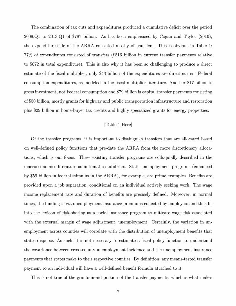
The combination of tax cuts and expenditures produced a cumulative deficit over the period

2009:Q1 to 2013:Q1 of $787 billion. As has been emphasized by Cogan and Taylor (2010),

the expenditure side of the ARRA consisted mostly of transfers. This is obvious in Table 1:

77% of expenditures consisted of transfers ($516 billion in current transfer payments relative

to $672 in total expenditure). This is also why it has been so challenging to produce a direct

estimate of the fiscal multiplier, only $43 billion of the expenditures are direct current Federal

consumption expenditures, as modeled in the fiscal multiplier literature. Another $17 billion is

gross investment, not Federal consumption and $79 billion is capital transfer payments consisting

of $50 billion, mostly grants for highway and public transportation infrastructure and restoration

plus $29 billion in home-buyer tax credits and highly specialized grants for energy properties.

[Table 1 Here]

Of the transfer programs, it is important to distinguish transfers that are allocated based

on well-defined policy functions that pre-date the ARRA from the more discretionary alloca-

tions, which is our focus. These existing transfer programs are colloquially described in the

macroeconomics literature as automatic stabilizers. State unemployment programs (enhanced

by $59 billion in federal stimulus in the ARRA), for example, are prime examples. Benefits are

provided upon a job separation, conditional on an individual actively seeking work. The wage

income replacement rate and duration of benefits are precisely defined. Moreover, in normal

times, the funding is via unemployment insurance premiums collected by employers and thus fit

into the lexicon of risk-sharing as a social insurance program to mitigate wage risk associated

with the external margin of wage adjustment, unemployment. Certainly, the variation in un-

employment across counties will correlate with the distribution of unemployment benefits that

states disperse. As such, it is not necessary to estimate a fiscal policy function to understand

the covariance between cross-county unemployment incidence and the unemployment insurance

payments that states make to their respective counties. By definition, any means-tested transfer

payment to an individual will have a well-defined benefit formula attached to it.

This is not true of the grants-in-aid portion of the transfer payments, which is what makes

7

them interesting to study formally. These are payments made principally to state and local

governments who have considerable latitude in terms of the allocations. Educational grants,

which amounted to $76 billion, are prime examples. The Department of Education stipulated

broad educational policies as a condition for states to receive funding based on a proportion

of their populations. They also stipulated that the states should provide assurances of intent

to return educational funding levels to those of fiscal year 2006 and maintain those funding

levels from fiscal year 2009 to 2011. Notice that these funding guidelines would not apply on

a county-by-county basis. However, all states supplement funding deficiencies at the local level

with the objective of moving toward more equal funding per pupil statewide than local revenues

might allow. Local funding deficiencies would be particularly acute during a contraction of the

intensity experienced during the Great Recession. Some states have such equalization formulae

embedded in their constitutions. Notice that this channel should manifest in the relationship

between public sector wage shocks and ARRA transfers. This will motivate the distinction

between unexpected changes in private and public wages in our policy function estimation.

The final category, temporary tax provisions, in the amount of $281 billion are excluded from

our analysis, but are briefly discussed here for completeness. About half of this amount funds

the Making Work Pay program and related tax credits provisions. One component is a 6.2%

individual income supplement up to $400, with a phaseout dollar-for-dollar above incomes of

$75K (thus reaching zero at $95K). Almost all counties would have qualified for the same $400

per capita tax cut, leaving no cross-sectional variation to relate to the risk-sharing channel that

is our focus.6

We turn now to a description of the ARRA grants in terms of their timeline of disbursements

and variation across counties.

3.2 The Distribution of Grants-in-Aid Across Counties

The purpose of this section is to document the extent to which per capita grants-in-aid transfers

were unequal across counties. Toward this end, the upper panel of Figure 1 presents the cross-

6) Of course the within county income distribution would be needed to assess the within county redistributiveeffect of this tax policy.

8

sectional distribution of the flow expenditure of ARRA grants-in-aid using a box and whisker

plot for each quarter of our micro-data (2009:Q3 to 2013:Q3).

Beginning with the cross-county median disbursements (the horizontal lines in the shaded

boxes), we see a gradual build-up in the first 5 quarters and then a tapering thereafter. By the

first quarter of 2012, the flow has fallen to a negligible amount and remains there going forward.

As measured by the median flows, the grants-in-aid are economically substantial in the first two

years of the program, averaging about 1.5% of median income per quarter.

Also very evident is variation around the median. The interquartile range (shared area) is

vast, ranging from a low of $21 per capita to a high of $168 in the third quarter of 2009 (this

translates to a range of 0.2 % to 1.3 % of median flow income).

[Figure 1 Here]

The lower panel presents the cumulative flows by county and again presents the quarter-by-

quarter cross-sectional distribution in a box and whiskers plot. At the time the funds have been

fully disbursed in 2013:Q3, the median county has received about $981 per capita, which amounts

to about 6.9% of median quarterly flow income, and is thus equivalent to a constant 0.43% of

median annual income in flow terms, over the duration of the program. The interquartile range

in 2013:Q3 is vast, $908 dollars, or around 6.4% of quarterly income.

Given our focus on county-level business cycles and risk-sharing, it is helpful to display

the raw inputs to our fiscal policy estimation on a map. The upper panel of Figure 2, plots the

cumulative wage income shocks (estimation details follow in the next section) from peak to trough

based on the official NBER dates (2007:Q4 to 2009:Q2). There is, perhaps not surprisingly,

considerable diversity of business cycle conditions across U.S. counties. More surprising, is the

fact that a large number of – admittedly sparsely populated – counties that experience positive

wage shocks during the Great Recession.

[Figure 2 Here]

The lower panel shows the cumulative ARRA transfers per capita. The median county thus

received about $981 per capita of transfers in total. This amounts to around 6.9% of the

9

quarterly flow of income over this period, for the median county. Consistent with the earlier

timeline of distributions there is enormous variation in the cross-section. Our focus is the

relationship between transfers to counties and the unpredictable, cyclical movements in wage

income. To get at this issue, one needs a model of county-level wage income dynamics, to which

we now turn.

4 County and National Business Cycles

As far as we know, there has been no systematic study of county-level business cycles or their

relationship to the national business cycle. This section intends to fill this gap as a necessary

preliminary step to estimating a fiscal policy function at the county level.

4.1 Wage Income Specification

Our preferred specification is a trend stationary model at the national and county level of

aggregation. This is consistent with the view that policymakers at the national level aim to

reduce cyclical variation in U.S. output relative to its historical trend growth rate.7

Beginning with a representative county, i, real wage income per capita is assumed to follow:

wit = αi + γit+ Γit2 + ρiwi,t−1 + λiεt + εit. (1)

The presence of lagged wage income captures the well-known feature of macroeconomic data that

departures from trend growth tend to be positively correlated over time (i.e., we expect ρi > 0).

Here, persistence is allowed to vary across counties. While we find a strong central tendency in

the persistence parameter across counties, as a practical matter, leaving them unrestricted helps

to ensure that forecast errors are not biased by arbitrarily assuming a common persistence level

across structurally diverse counties.

7) An earlier version of this paper also examined difference-stationary specifications and found evidence ofover-differencing. Moreover, first-differencing is known to exacerbate measurement error, particularly in finelydisaggregated data. This would lead to significant attenuation bias in the fiscal policy estimates where shocks toincome are the regressors.

10

Notice that the residual in this regression, εit is indexed by county i and period t, the same

two dimensions of the data panel itself. Obviously, this is a mechanical implication of panel

econometrics: there will always be unexplained variation at the unit of observation, thus εit is

completely standard. The more novel and interesting facet of the specification is the presence

of the common shock, εt, which carries a county-specific factor loading, denoted by λi. In

words: the common shocks shift the entire cross-county wage distribution, generating perfect

multicollinearity among all counties. Factor loadings exceeding 1 indicate an amplified business

cycle response to a common shock while values less than 1 indicate dampening. It is worth

noting that negative factor loadings, which would identify counties with local business cycles

that are counter-cyclical to the national business cycle, are rare.

The common shocks are estimated from a first-stage regression using the average of wit

across the entire distribution of 3,133 counties. The cross-county average is denoted by wt.

The empirical specification for the average wage takes the same functional form as that of an

individual county:

wt = α + γt+ Γt2 + φwt−1 + εt . (2)

Equation (2) provides a natural benchmark with which to estimate the common, macroeconomic

shock, εt, that shifts the mean of the county-level wage income distribution. Notice, if the

persistence parameters are the same across counties in equation (1), the county-level specification

aggregates exactly to produce equation (2), with the factor loading parameters averaging to unity

across counties and the county-specific shocks averaging to zero. This is not just a theoretical

curiosity, it appears to be the case in practice: the persistence of the mean wage income process,

φ, is 0.75, indistinguishable from the persistence of the median county at 0.77. The average and

median of the factor loadings are indistinguishable from 1, at 0.99 and 1.01, respectively.

Turning to the details, we estimate this pair of equations for each county using OLS with

Newey-West robust standard errors to account for potential auto-correlation and heteroscedas-

ticity in the error terms. In the first step, we estimate the aggregate wage income equation (2)

and save the estimated common shocks εt. Then, we estimate (1) county-by-county, inserting

11

the estimated common shocks, εt, from the first step.

This two-step process has the desirable feature that the common shock is orthogonal to the

county-specific shock. The upshot is that counties now have two sources of wage income risk:

1) one due to cross-county heterogeneity in county-level wage responses to the common shock,

λiεt, and 2) one due to the county-specific shocks, εit.

Note, some care should be taken when interpreting the county-specific shock. While this

shock has the desirable property that it is orthogonal to the common shock by construction,

the pairwise correlations of εit structure are left unrestricted. To be concrete, consider the

recent fracking boom. Over the last few decades, an increasing number of counties have become

substantially dependent on wage income from fracking. This inevitably gives rise to a common

shock, within the sub-group of counties highly dependent on fracking income, not shared by

other counties. At the same time, as a sufficiently large number of counties engage in fracking,

the general equilibrium impact of the aggregate fracking boom, while raising relative wages in

fracking counties, could lower the GDP price deflator, through energy price declines, for both

fracking and non-fracking counties. This equilibrium effect would be part of the common shock

and would be expected to have a much larger loading on the counties directly earning wages

from fracking, compared to those benefiting indirectly from the positive spillover of lower energy

prices.

Our two-step approach recovers several parameters and shocks of potential interest: 1) the

intercept αi; 2) the linear and quadratic trend coefficients, γi and Γi; 3) the persistence of

the county-level wage income process, ρi; 4) the factor loading on the common shock, λi; 5) a

historical sequence of estimated common shocks, εt; and 6) a historical panel of county-specific

shocks, εit.

Our use of the phrase ‘of potential interest’ is intentional. Our focus on business cycle

variation leads us to treat the trend terms as nuisance parameters, needed to induce stationary

in real wage incomes. The constants are also not very interesting unless the trends are equal, or

approximately so, in which case they translate into estimates of long-run wage income differences

across counties. For these reasons, the discussion that follows will focus on the persistence

12

parameters, the factor loadings, and the shock sequences.8

4.2 Estimation Results

Turning to the estimation results, Table 2 summarizes the parameter estimates: both their

averages across counties and the extent of heterogeneity across counties.

The median county has a wage income persistence of 0.77 (a half-life of about 2.65 quarters).

As might be expected, there is considerable variation in persistence around the median: from

0.66 to 0.84, based on the 25th and 75th percentiles of the estimated distribution. These estimates

translate into half-lives with a range of 1.69 quarters to 3.97 quarters.

[Table 2 Here]

As first emphasized by Baxter and Crucini (1995), what is important from a welfare perspec-

tive when comparing locations – in their case, nations, in our case, counties – is the persistence

of the productivity gap. The productivity gap (holding fixed inputs of capital and labor) maps

directly in the relative income and wealth effects through the intertemporal budget constraint.

Moreover, high persistence in the labor productivity gap has two effects. On the capital accu-

mulation side, it makes reallocation of capital more compelling than the case of highly transitory

shocks. This amplifies the wealth effects of the productivity movements across locations. On

the labor input side, more persistence tends to bring about more balance in the wealth and

substitution effects of labor supply decisions.9

In our context, the gap in persistence based on the estimated inter-quartile range is only 0.18

(0.84-0.66 for total wages) which translates into a predicted wage income gap of only 3.2% after

just one quarter following a common 10% income shock. In summary, persistence heterogeneity

appears not to be an important quantitative feature of the sources of gains from risk-pooling

across counties.

8) The full distributions of the parameter estimates across counties are presented in a series of kernel densityestimates in the estimation appendix.9) Note that these differences are likely to be magnified in the context of the Great Recession due to the financialshocks that negatively impact the ability of agents to pool risk through credit markets (see, for example, Perriand Quadrini (2018)).

13

The heterogeneity of business cycle experiences across counties, therefore, falls to differences

in the factor loadings on the common shock and the variability of the county-specific shocks. The

county-level parameter estimates indicate that both of these stochastic features are important

sources of business cycle heterogeneity across counties.

For the median county, the standard deviation of the idiosyncratic shock is 2.97% (Table 2).

The median factor loading (λi) on the macroeconomic shock is indistinguishable from unity at

1.01. This, combined with the fact that the common (macroeconomic) shock has a standard

deviation of 1.3%, implies that for the median county, the microeconomic shocks account for

two-thirds of the variation, while the macroeconomic shock accounts for the remaining one-third.

Keeping in mind that the county-specific shock is likely to contain measurement errors which

are averaged away in the construction of the macroeconomic shocks, the estimated contribution

of the microeconomic shock might better be viewed as an upper-bound.

There is considerable county-level heterogeneity in factor loadings and county-specific shock

variances. Beginning with the microeconomic shock (εit), the standard deviation ranges from

2.22% to 4.21%, a factor of 1.9. The factor loadings on the common shock (λi) range from

0.6 to a high of 1.35 (moving from the 25th to 75th percentile cutoffs). In words, a negative

5% macroeconomic wage income shock (comparable to the Great Recession) would induce a 3%

decline in county-level wages in the former case and a 6.75% wage decline in the latter case. This

parameter range is a factor of about 2.1, slightly greater than the cross-county heterogeneity

found in volatility associated with the county-level shocks.

As part of our robustness analysis, we consider a split of wage income into private wage income

and public wage income. Due to some inconsistencies in the reporting of public wages by county

in the QCEW, we compute total public wage income as the difference between total county wage

income and total private wage income. Estimates of the parameters for the stochastic processes

for private and public wages by county are also reported in Table 2. What is most notable about

the split is that the parameters and shock variances are actually quite similar across the private

and public sectors. As one might expect, the innovations to private and public wages tend to be

more volatile than the two combined, indicative of some diversification benefits of having both

14

income streams in the county. In the lower panel, we see the standard deviation of total wages

has a cross-county median of about 3%, while private and public wages have standard deviations

of about 3.5% each.

4.3 Forensic Analysis of the Great Contraction

Our identification of the fiscal federalism and risk-sharing channel will exploit the timing of

the contraction relative to the passage of the ARRA and disbursement of funds. This will be

discussed further in the next section.

To get a sense of the cumulative misery brought about by the Great Recession across counties,

Figure 3 presents the distributions of the cumulative wage income shocks by type of shock and

wage measure. The top panel shows the cross-county distributions of common and county-level

shocks, in red and gray bars, respectively. The lower two panels are the shocks estimated from

the private and public wage series, when estimated separately.

[Figure 3 Here]

Beginning with total wages, the cumulative shocks over the Great Recession amounted to

-4.6%, while the corresponding values for private and public wages were -8.8% and +2.8%,

respectively. These cross-county means are clearly visible in the central tendencies of the cross-

county distributions of the common shocks. The fact the public wages were, on average, above

trend during the contraction is interesting and, as we shall see, gives rise to an implication that

transfers are positively correlated with the common shock component of public sector wages.

The county-level shocks are very close to mean zero across counties though considerably more

dispersed than the factor loadings on the common shocks (i.e., the dispersion of wage income

associated with the common shock). The county-level shocks for public wages are evidently

much more compressed than their private counterparts. This could reflect the fact that while

school districts are institutionally organized on a county level, teachers’ unions exist at the state

and the national level.

15

5 Fiscal Federalism

The theoretical concept of fiscal federalism covers a range of fiscal issues spanning political

jurisdictions, but a key element involves transfers from the national government to sub-national

governments. From the perspective of the question posed in this paper concerning risk-sharing,

these transfers should be place-based and state-contingent. That is, they should help counties

most affected by the Great Recession.

5.1 What is Fiscal Federalism?

The most transparent example of fiscal federalism is Canada’s system of equalization payments

from the national government to the provincial governments. Effectively, equalization payments

transfer federal funds from provinces with higher fiscal capacity to those with lower fiscal ca-

pacity. In the Canadian system, there is both a long-run equalization effect and a business

cycle effect. That is, equalization payments, when averaged over time will reflect the permanent

inter-provincial income inequality and will thus reduce the dispersion of wage income in the

long run.10 Equalization payments in any given year, relative to these long-run means, will be

a function of the relative movements of wage income (and thus tax revenue and fiscal capacity)

across provinces in that year. For example, energy prices are of enormous influence given the

concentration of the oil sands in the provinces of Alberta (and to some extent Saskatchewan).

These provinces have higher income, on average, over time compared to other provinces, but

much more so when oil prices are over $100 per barrel than at less than $50.

Thus, from the perspective of helping counties most affected by the Great Recession, con-

ceptually the appropriate model is the state-contingent transfer system associated with fiscal

federalism. That is, to assess the potential role of risk-pooling through fiscal federalism we must

determine how relative economic conditions across U.S. counties enter into the determination of

the transfers they receive.

From a rational expectations perspective, this leads to a pernicious identification issue similar

10) The reduction in post-transfer income inequality requires that the distortionary effects not outweigh thedirect effects of the transfers and thus hinge on the magnitude of equilibrium wealth and substitution effects.

16

to that faced when economists estimate the reverse regression, with changes in GDP on the

left-hand side and changes in government consumption on the right-hand side. That is, when

attempts are made to estimate the fiscal multiplier. We turn, now, to a discussion of this issue

and how we propose to resolve it in the context of the ARRA.

5.2 Identification

In the fiscal multiplier context, when output falls unexpectedly due to an unidentified (or par-

tially identified) shock, the unconditional covariance between changes in output and government

spending suffers from negative simultaneity bias. The negative macroeconomic shock induces a

discretionary increase in government consumption. Causation runs from the business cycle shock

to the policy response. Government consumption, in turn, may have mitigated the impact of

the shock. Causation also runs from government consumption to wage income. With causation

running in both directions, simply regressing the change in output on the change in government

consumption, the fiscal multiplier is downward biased (assuming the true impact of an exoge-

nous change in government consumption on wages positive). This line of reasoning leads to the

common claim: “things would have been worse in the absence of the fiscal stimulus.”

The grants-in-aid are transfers to state and local governments (as well as to non-profits

and firms), not Federal government consumption, so they clearly increase the level of financial

resources in a county relative to when they are absent. This is, of course, our and Dupor (2014)’s

rationale for conducting a forensic analysis of the allocation of ARRA transfers to individual

counties and over time. Without accurate tracking, the income effects of the transfers will

not be attributed to the correct recipient, or in our case, the correct county. Moreover, once

the funds are spent on goods and services, the subsequent indirect economic effects via the

traditional fiscal multiplier will also not be correctly identified in terms of the final expenditure

multipliers. The issue is further complicated by the fact that the ARRA policy (as described

in the state objectives) calls for a response to both an aggregate shock and a local shock with

the final expenditure rarely taking the form of homogeneous federal consumption (e.g., military

spending).

17

As it turns out, this particular episode in U.S. history presents something of a natural

experiment in fiscal federalism. As a matter of fact, the contractionary phase of the Great

Recession predates the passage of the stimulus bill. Moreover, the actual disbursement and

expenditure of funds occurs with even greater delays, beyond the business cycle trough, as they

are typically based upon discretionary decisions by the primary (often the state government)

and secondary recipients. This timing structure provides our identification strategy whereby

the policy function determines the post-recession cumulative allocation of grants-in-aid received

by an individual county as a fraction of the cumulative unexpected declines of wage income

experienced by that same county, during the contraction.11 We call this a fiscal federalism

offset, or fiscal offset, for short.

[Figure 4 Here]

The fact that the negative wage income shocks pre-date the ARRA stimulus package and

the flow of transfers is clear from Figure 4. The upper panel presents the distribution of wage

shocks across counties and over time. The dark red solid line is the median shock across counties,

the dark shaded area is the inter-quartile range of shocks and the light red shaded area is the

distribution of the shocks from the 5th percentile to the 95th percentile. For completeness and

ease of presentation, the shocks displayed here are the composite of the macroeconomic and the

microeconomic shocks, λiεt + εit, which we call the composite shock in what follows.

The lower panel shows the distribution of grants-in-aid disbursements to the counties (the

lines and color-coding follows those of the upper panel). These disbursements, too, were discussed

earlier in great detail. The key takeaway here, however, is the timing of transfers relative to the

negative wage income shocks. Remarkably, the contractionary phase (the shaded area) of the

Great Recession is basically complete at the time the ARRA funds begin to flow.

Our fiscal risk-sharing policy function exploits this timing sequence by regressing the cu-

mulative post-contraction transfers to each county from 2009:Q3 to 2013:Q3 on the cumulative

11) An earlier version of this paper used contemporaneous transfers and business cycle shocks throughout thedisbursement period of ARRA. We are grateful to the editor, Vincenzo Quadrini, and an anonymous referee forpressing us to develop a more effective identification strategy.

18

income shocks during the contraction, 2007:Q4 to 2009:Q2. Since the timing of disbursements

and their cross-county distribution were not known at the time of U.S. business cycle contraction,

the wage income shocks during the contraction are exogenous to the post-contraction ARRA

transfers. With this one-way causality from past wage income shocks to future transfers, we are

able to answer the question posed in the title.

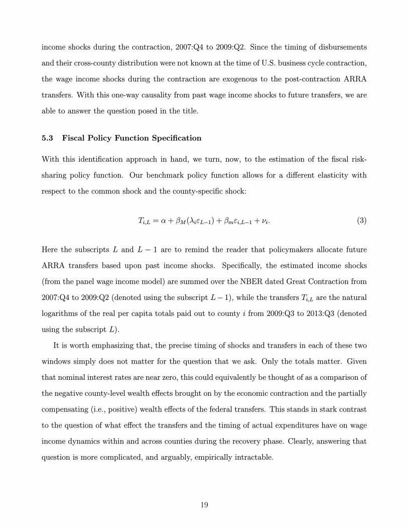
5.3 Fiscal Policy Function Specification

With this identification approach in hand, we turn, now, to the estimation of the fiscal risk-

sharing policy function. Our benchmark policy function allows for a different elasticity with

respect to the common shock and the county-specific shock:

Ti,L = α + βM(λiεL−1) + βmεi,L−1 + νi. (3)

Here the subscripts L and L − 1 are to remind the reader that policymakers allocate future

ARRA transfers based upon past income shocks. Specifically, the estimated income shocks

(from the panel wage income model) are summed over the NBER dated Great Contraction from

2007:Q4 to 2009:Q2 (denoted using the subscript L− 1), while the transfers Ti,L are the natural

logarithms of the real per capita totals paid out to county i from 2009:Q3 to 2013:Q3 (denoted

using the subscript L).

It is worth emphasizing that, the precise timing of shocks and transfers in each of these two

windows simply does not matter for the question that we ask. Only the totals matter. Given

that nominal interest rates are near zero, this could equivalently be thought of as a comparison of

the negative county-level wealth effects brought on by the economic contraction and the partially

compensating (i.e., positive) wealth effects of the federal transfers. This stands in stark contrast

to the question of what effect the transfers and the timing of actual expenditures have on wage

income dynamics within and across counties during the recovery phase. Clearly, answering that

question is more complicated, and arguably, empirically intractable.

19

More elaborate specifications are also considered, including:

Ti,L = α + βsM(λsiε

sL−1) + βs

mεsi,L−1 + νsi , (4)

where s indexes either the private or public sector and thus allows for sector-specific shocks

of each type. Note that both the factor loadings and the policy response coefficients are also

sector-specific.

Finally, we also estimate a policy function with all four sources of shocks included (pri-

vate common, private county-specific, public common, and public county-specific). The policy

function with all the types of shocks allows a somewhat greater amount of the transfers to be ex-

plained, but the coefficients of the policy function remain largely unaffected because the shocks

are not highly correlated across counties.

In reporting estimation results, the estimated coefficients are standardized in the usual sense:

they indicate how a one standard deviation wage income shock moves transfers in units of its

standard deviation. Of course, the transfers still have the interpretation of a percentage offset

of the negative wage income shocks during the contraction, in the total income of the county.

The standardization makes it clear that the policy function is an elasticity with respect to the

shock and does not depend on the scale of the shock. This can be seen by noting that without

standardized coefficients, if one multiplies the factor loading by a larger macroeconomic shock

(εt), the effect on a non-standardized coefficient will be to reduce the slope parameter by the

same proportion. Whereas with the standardized coefficient, the slope parameter is invariant to

the size of the shock.

The same logic reveals an additional, desirable, feature of our approach. The identification

of the elasticity of the transfer policy function with respect to the macroeconomic shock arises

exclusively from the covariance of λi and TiL. Since the factor loadings are historical features

of the cross-sectional county wage income process, they are not parameters that are endogenous

to the ARRA transfers themselves. This provides an additional source of identification for the

redistributive role of the transfers. Note, that the same is not true of the microeconomic shock

20

and thus the timing convention we employ remains crucial from that perspective.

What then is the role of the macroeconomic shock? First, the sign of the shock is important

since transfers are strictly positive. So, the expectation is a negative coefficient such that when

the economy is contracting, positive transfers are made. Second, the size of the common shock

determines the size of the appropriation necessary to provide the proportional offset. Third,

the more afflicted the county is by the common shock (i.e., the larger is λi), the higher is the

absolute size of the per capita transfer.

Sensibly, if the macroeconomy is not in a recession, in the sense that εt = 0, there is no justi-

fication for discretionary spending, associated with the common shock. No aggregate appropria-

tion. There will still be purely redistributive transfers to offset the county-specific shocks. This

is what happens in general with fiscal federalism, as in the case of Canada. Provinces contribute

different amounts to national tax revenue streams given the conditions of their economies and

the federal taxes they remit and the equalization payments represent net-zero aggregate transfers

and thus a vector of positive and negative transfer payments on a province-by-province basis.

In the U.S. case, this would only be operative for discretionary spending when the appropri-

ation is explicitly intended to redistribute, which is just one of the stated goals of the ARRA.

Thus, we can think of the ARRA as the first historical experiment in fiscal federalism by the

U.S. federal government and the estimated policy function is only appropriate for the Great

Recession.

Notice that, by definition, the idiosyncratic shocks average toward zero across counties and

thus define a set of taxes and subsidies that net to zero within each quarter. In contrast, the

transfers associated with the macroeconomic shock are strictly positive (since, as we shall see,

the betas are negative). That is, grants add to the Federal deficit during the Great Recession due

to the offset of macroeconomic shocks (λi). These deficits would need to be financed using some

combinations of future tax increases and spending reductions. Whatever the excess burden of

the ARRA may be (due to these deficit-balancing actions), the point of this paper is to determine

if the current beneficiaries are those most affected by the Great Recession.

Thus βM < 0 is the percentage offset of the cumulative effect of the common shock on county

21

i.12 Notice that the cumulative effect on the median (or average) county is, quite sensibly, just

the cumulative shocks experienced by the aggregate economy (i.e., λi = 1 on average). However,

the dollar offset is larger (smaller) in absolute terms for counties that amplified (muted) responses

to the common shock, λi > 1 (λi < 1).

Turning to the microeconomic shock, the cross-county income variance brought about by the

sequence of microeconomic shocks during the Great Contraction is εi,L−1. Adding the transfer

flows to these shocks gives us: (1 + βm)εi,L−1. Thus, βm < 0 is the percentage offset of the

cumulative microeconomic shocks experienced by county i during the contraction.

Understanding the risk-sharing facet of the offset requires a focus on the second moment

of the distribution of the shock distribution. Consider, again, the common shock. During

the contraction, total wage income fell, on average (across counties), by 4.9%. The dispersion

arises not from the shock, but from the implications of the shock given the heterogeneity in

factor loadings. Simply put, the conditional variance of income across counties brought about

by the common shock is vari(λi) multiplied by the square of the shock. In contrast, for the

microeconomic shock, the mean across counties is zero. It is the dispersion of the εi,L−1 across

i that determines the change in wage income dispersion arising from these shocks, during the

contraction.

5.4 Estimation Results

We turn, now, to the policy function estimates. Keep in mind, as discussed in the previous

section, the estimated coefficients in the table are standardized.

Table 3 reports the results of the policy function estimation. The top panel uses the shocks

recovered from total wages, the middle panel uses the shocks recovered from private wages and

the bottom panel uses the shocks recovered from public wages.13 Bootstrapped standard errors

12) In principle, we could make a small adjustment to account for the fact that the present value of the dis-bursements is lower when discounted back to the period of the shocks. We choose not to do so because theadjustment would be small and somewhat arbitrarily assume a common discount rate across counties. Thus weprefer the more transparent comparison of simple cumulative real per capita values across relatively proximateperiods without arbitrary adjustments for discounting flows.13) In all specifications, zero-dollar ARRA transfers are replaced with a small positive value to avoid taking thelog of zero. Excluding the zeros has very little impact on the coefficients of the estimated policy function.

22

are reported to account for the use of generated regressors (i.e., the estimated shocks from the

wage income estimation).

[Table 3 Here]

We use the term fiscal offset to refer to the coefficients on the policy function. The intuitive

rationale is that the coefficient represents the proportional change in cumulative county wage

income shocks during the contraction that is offset by cumulative flows the county receives under

the ARRA. This gives a well-defined answer to a well-defined question.

Beginning with total wages in the top panel of the table, the first row shows the fiscal offset

coefficient to be -10.3%; that is, a 10% “shock” at the county level will be reduced to 8.97%.

The next two rows separate the common (macro) shock from the idiosyncratic county micro

shock. The value of distinguishing the two shocks is immediately evident since the offset of the

common shock is 1.6 times that of the offset of the county-specific shock, -13.7% versus -8.5%

(column 3). The last column includes both shocks in the same policy function. The coefficients

are very similar to the case when they are estimated in separate regressions, due to the fact that,

period-by-period, the county-specific shock is orthogonal to the common shock.14

If the private and public sectors experience different shocks, then it is important to consider

if the policy function is misspecified when they are aggregated together. This possibility is easily

accommodated by the fact that we estimated separate wage equations for the private and public

sectors. These policy function estimates are presented in the middle and lower panels of Table

3.

Beginning with the composite private shock and composite public shock, we see that for

private wages the coefficient is now indistinguishable from zero while the coefficient for the com-

posite public wage shock is negative, economically and statistically significant, and comparable

in magnitude to its counterpart for the results using the aggregate wage, -12.5% offset predicted

versus -10.3% in the first row of panel A. While it is tempting to suggest that this shows that

the public sector and not the private sector benefited from the transfer policies, this is not an

14) Readers familiar with omitted variable bias will appreciate this demonstration of unbiasedness in the contextof omitted, uncorrelated, regressors.

23

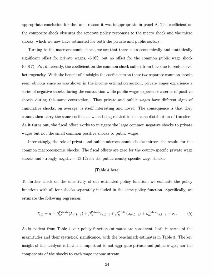
appropriate conclusion for the same reason it was inappropriate in panel A. The coefficient on

the composite shock obscures the separate policy responses to the macro shock and the micro

shocks, which we now have estimated for both the private and public sectors.

Turning to the macroeconomic shock, we see that there is an economically and statistically

significant offset for private wages, -6.9%, but no offset for the common public wage shock

(0.017). Put differently, the coefficient on the common shock suffers from bias due to sector-level

heterogeneity. With the benefit of hindsight the coefficients on these two separate common shocks

seem obvious since as was shown in the income estimation section, private wages experience a

series of negative shocks during the contraction while public wages experience a series of positive

shocks during this same contraction. That private and public wages have different signs of

cumulative shocks, on average, is itself interesting and novel. The consequence is that they

cannot then carry the same coefficient when being related to the same distribution of transfers.

As it turns out, the fiscal offset works to mitigate the large common negative shocks to private

wages but not the small common positive shocks to public wages.

Interestingly, the role of private and public microeconomic shocks mirrors the results for the

common macroeconomic shocks. The fiscal offsets are zero for the county-specific private wage

shocks and strongly negative, -13.1% for the public county-specific wage shocks.

[Table 4 here]

To further check on the sensitivity of our estimated policy function, we estimate the policy

functions with all four shocks separately included in the same policy function. Specifically, we

estimate the following regression:

Ti,L = α + βPrivateM (λiεL−1) + βPrivate

m εi,L−1 + βPublicM (λiεL−1) + βPublic

m εi,L−1 + νi . (5)

As is evident from Table 4, our policy function estimates are consistent, both in terms of the

magnitudes and their statistical significance, with the benchmark estimates in Table 3. The key

insight of this analysis is that it is important to not aggregate private and public wages, nor the

components of the shocks to each wage income stream.

24

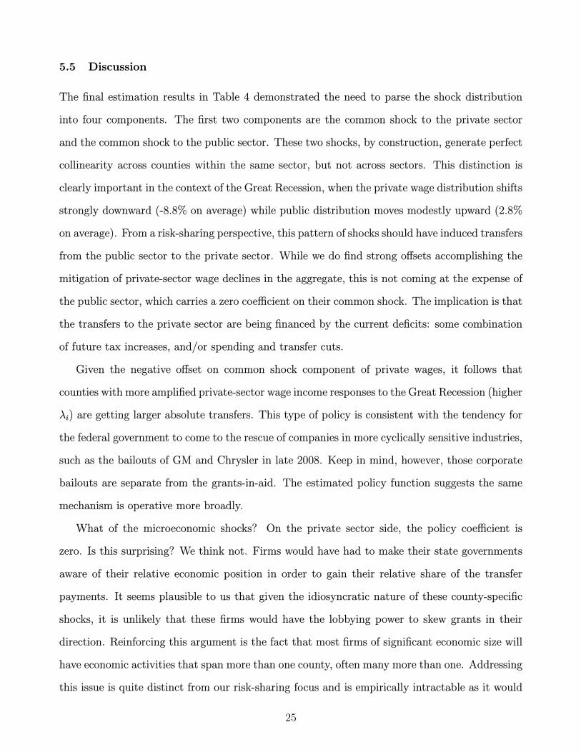
5.5 Discussion

The final estimation results in Table 4 demonstrated the need to parse the shock distribution

into four components. The first two components are the common shock to the private sector

and the common shock to the public sector. These two shocks, by construction, generate perfect

collinearity across counties within the same sector, but not across sectors. This distinction is

clearly important in the context of the Great Recession, when the private wage distribution shifts

strongly downward (-8.8% on average) while public distribution moves modestly upward (2.8%

on average). From a risk-sharing perspective, this pattern of shocks should have induced transfers

from the public sector to the private sector. While we do find strong offsets accomplishing the

mitigation of private-sector wage declines in the aggregate, this is not coming at the expense of

the public sector, which carries a zero coefficient on their common shock. The implication is that

the transfers to the private sector are being financed by the current deficits: some combination

of future tax increases, and/or spending and transfer cuts.

Given the negative offset on common shock component of private wages, it follows that

counties with more amplified private-sector wage income responses to the Great Recession (higher

λi) are getting larger absolute transfers. This type of policy is consistent with the tendency for

the federal government to come to the rescue of companies in more cyclically sensitive industries,

such as the bailouts of GM and Chrysler in late 2008. Keep in mind, however, those corporate

bailouts are separate from the grants-in-aid. The estimated policy function suggests the same

mechanism is operative more broadly.

What of the microeconomic shocks? On the private sector side, the policy coefficient is

zero. Is this surprising? We think not. Firms would have had to make their state governments

aware of their relative economic position in order to gain their relative share of the transfer

payments. It seems plausible to us that given the idiosyncratic nature of these county-specific

shocks, it is unlikely that these firms would have the lobbying power to skew grants in their

direction. Reinforcing this argument is the fact that most firms of significant economic size will

have economic activities that span more than one county, often many more than one. Addressing

this issue is quite distinct from our risk-sharing focus and is empirically intractable as it would

25

require aggregating the grants-in-aid by firm size and considering the shocks impacting firms

based on their sector of specialization and geographic reach.

On the public sector side, the mechanisms are very different. Given the large component

of education funding in the stimulus package and the fact that all state governments have a

responsibility to keep educational funding per pupil more equal, it is natural that revenue short-

falls in various school districts should be met with redistributive transfers that depend on their

relative economic conditions. Moreover, since K-12 school districts are typically organized along

county lines, our spatial aggregation is particularly well suited to identify this facet of the ARRA.

6 Robustness

This section reports additional results that alter our benchmark analysis in a number of ways

to check on their robustness and our interpretations of the findings.

6.1 Sensitivity Analysis: Allocations of Grant-in-aid

An important contribution of our paper is tracking the funds appropriated by the U.S. Congress

all the way to end recipients at the zip-code level. The process by which this occurs starts with

the Federal Agencies and Departments charged with their specific appropriations and more often

than not involves delegation to state and local governments to intermediate the process with

considerable discretion about the details. Inevitably, there are delays in the movement of funds

from the state level and beyond. At times, there is less than complete or accurate reporting of

the allocations. This leads to the potential for geographic misallocation of funds in the panel

data.

To consider this possibility, we explore the extent to which the estimated parameters of the

policy function are sensitive to leaving counties out of the panel estimation, one at a time. Given

the large appropriations allocated to state capitals and the dominant role of state governments

in subsequent allocations, we also consider the implications of leaving out all counties in which

a state capital resides.

26

The re-estimated coefficients, presented in Figure 5, are normalized by the corresponding

estimates using the full sample in Table 3. Thus, a value of 1.01 means the coefficient is 1%

higher when a county is left out of the pooled estimate. The distribution of the resulting

estimates is presented both in the form of histograms and smoothed kernel density estimates in

Figure 5.

Overall, we find that our benchmark estimates are basically invariant to the exclusion of a

randomly chosen county. The aggregate fiscal offset (panel A) has a median value of around

1.001, with the majority of these “leave-one-county-out” estimates remaining close to the median

(most of the estimates range between 1 and 1.005). This result implies that leaving out counties,

one by one, does not have a material effect on the policy function estimates. In panels B and C

of Figure 5, it is also clear that the offset coefficient for common shocks to private wages and to

microeconomic shocks to public wages are robust to leaving out counties one by one.

We next turn to the counties in which the state capitals are located. The estimates for the

samples that leave out all state capitals are presented as the vertical lines in Figure 5. Here

the estimates are once again adjusted by the corresponding benchmark with the full sample. As

is evident in Figure 5, the coefficients are, again, virtually unaffected: leaving out the capital

counties only skew our estimates by at most 3% for the case of composite fiscal offsets.

[Figure 5 Here]

6.2 Fiscal Offsets and the Sizes of ARRA Transfers

We next explore the extent to which our estimates of the effects of the ARRA program in

offsetting income shocks at the county level are sensitive to the size of the transfers. To that

end, we estimate specification (1) of Table 4 and report the estimates of the common, and

county-level policy functions for private, and public wages at different quantiles (10th to 90th) of

the per capita transfer distribution. Specifically, we estimate these specifications using quantile

regression with the Epanechnikov kernel and the Hall et al. (1991) bandwidth selection. We

report 95% confidence bands (i.e., the shaded areas in Figure 6).

[Figure 6 Here]

27

The left panels show the fiscal offset parameters for the common shock while the right panels

show the offset parameters for the county-specific shock. The upper panel focuses on private

wages while the lower panel considers public wages. For reference, the fully-pooled benchmark

results are indicated by the horizontal line with 95% confidence intervals. The point estimates

at each quantile of the size-distribution (per capita) are indicated by the dots with red-shaded

bands providing the 95% confidence intervals.

The key takeaway from this analysis is that it is not possible to reject the hypothesis that the

pooled estimates are valid across the entire distribution, stratified by per capita transfer levels.

This can be gleaned by looking for instances in which the two confidence intervals overlap. The

only case in which they do not is in panel D and, even there, it is isolated to the lowest percentile

of the distribution.

7 Conclusion

As Oh and Reis (2012) have correctly pointed out, much of the ARRA stimulus came in the form

of transfers rather than increases in government consumption. This paper studies the role of the

discretionary part of the stimulus in terms of mitigating wage income variance across counties,

finding evidence of a particularly strong fiscal offset of the asymmetric county-level responses to

the common shock to private wages and to the county-specific components of public wages.

It is important to note that the shocks to income after the stimulus bill is passed and funds

are disbursed are jointly determined by contemporaneous, endogenous, responses to the actual

disbursements, future shocks impinging on county-level wages, and the natural mean reversion

of county-level wage income toward its long-run trend. Attempting to deal with the simultaneity

of private and public expenditures arising from transfers at the county level is a more daunting

task and worthy of further investigation. Our linkage of transfers to wage income shocks during

the contract phase represents a first step in that direction.

Future work should aim at establishing a structural framework that can account for these

collinear, asymmetric-sized wage income movements. Doing so may suggest both an improve-

28

ment in the design of social insurance programs such as the unemployment insurance program

and also a more efficient allocation of discretionary funds such as the ARRA. The fact that the

policy function explains a small fraction of the observed cross-county variation in the ARRA

suggests that following the protocol of the empirical model developed here in the future could

bring about significant policy efficiency gains and thus more successes in helping counties most

affected by recessions as emphasized in the ARRA’s statement of objectives.

By the same token, it seems problematic to rely on models with a single representative agent

to guide the discussion of fiscal multipliers when redistributive effects of asymmetric allocations

inevitably arises. With asymmetric business cycles and incomplete markets, the fiscal multipliers

and optimal policies will look very different.

Much remains to be done.

Acknowledgement The authors thank seminar participants at the College of William and

Mary, Federal Reserve Bank of Richmond, Miami University, Oberlin College, Vanderbilt Uni-

versity, University of Cincinnati, and conference attendees at the Midwest Macroeconomics

Meetings.

References

Asdrubali, Pierfederico, Bent Sorensen, and Oved Yosha, “Channels of Interstate RiskSharing: United States 1963-1990,” The Quarterly Journal of Economics, 1996, 111 (4), 1081–1110.

Baxter, Marianne and Mario J. Crucini, “Business Cycles and the Asset Structure ofForeign Trade,” International Economic Review, 1995, 36 (4), 821–54.

Bohn, Henning, “”The American Recovery and Reinvestment Act: Solely a government jobsprogram?” - Comment,” Journal of Monetary Economics, 2013, 60 (5), 550–553.

Boone, Christopher, Arindrajit Dube, and Ethan Kaplan, “The Political Economy ofDiscretionary Spending : Evidence from the American Recovery and Reinvestment Act,”Brookings Papers on Economic Activity, 2014, (Spring 2014), 375–428.

Chodorow-Reich, Gabriel, Laura Feiveson, Zachary Liscow, and William Gui Wool-ston, “Does State Fiscal Relief During Recessions Increase Employment? Evidence from the

29

American Recovery and Reinvestment Act,” American Economic Journal: Economic Policy,2012, 4 (3), 118–45.

Cogan, John F and John B Taylor, “What the Government Purchases Multiplier ActuallyMultiplied in the 2009 Stimulus Package,” Working Paper 16505, National Bureau of EconomicResearch October 2010.

Conley, Timothy G. and Bill Dupor, “The American Recovery and Reinvestment Act:Solely a government jobs program?,” Journal of Monetary Economics, 2013, 60 (5), 535–549.

Dupor, Bill, Marios Karabarbounis, Marianna Kudlyak, and M. Saif Mehkari, “Re-gional Consumption Responses and the Aggregate Fiscal Multiplier,” St Louis’ Fed WorkingPaper, 2018, 1, 1–61.

Dupor, William, “The 2009 Recovery Act Directly Created and Saved Jobs Were Primarilyin Government,” Federal Reserve Bank of St. Louis Review, 2014, 2, 123–146.

Feyrer, James and Bruce Sacerdote, “Did the Stimulus Stimulate? Real Time Estimates ofthe Effects of the American Recovery and Reinvestment Act,” NBER Working Paper Series,2011, p. 16759.

Gimpel, James G., Frances E. Lee, and Rebecca U. Thorpe, “Geographic Distributionof the Federal Stimulus of 2009,” Political Science Quarterly, 2012, 127 (4), 567–595.

Goodman, Christopher J. and Steven M. Mance, “Employment loss and the 2007-09recession: an overview,” Monthly Labor Review, 2011, (April), 3–12.

Hall, Peter, Simon J. Sheather, M. C. Jones, and J. S. Marron, “On Optimal Data-Based Bandwidth Selection in Kernel Density Estimation,” Biometrika, 1991, 78 (2), 263–269.

Inman, Robert P, “States in Fiscal Distress,” Working Paper 16086, National Bureau ofEconomic Research June 2010.

Johnson, N., “Does the American Recovery and Reinvestment Act Meet Local Needs?,” Stateand Local Government Review, 2009, 41 (2), 123–127.

Leduc, Sylvain and Daniel Wilson, “Are State Governments Roadblocks to Federal Stimu-lus? Evidence on the Flypaper Effect of Highway Grants in the 2009 Recovery Act,” AmericanEconomic Journal: Economic Policy, 2017, 9 (2), 253–92.

Nakamura, Emi and Jon Steinsson, “Fiscal Stimulus in a Monetary Union: Evidence fromUS Regions,” American Economic Review, 2014, 104 (3), 753–792.

Oh, Hyunseung and Ricardo Reis, “Targeted transfers and the fiscal response to the greatrecession,” Journal of Monetary Economics, 2012, 59 (Supplement), S50 – S64.

Perri, Fabrizio and Vincenzo Quadrini, “International Recessions,” American EconomicReview, April 2018, 108 (4-5), 935–84.

Wilson, Daniel J., “Fiscal Spending Jobs Multipliers: Evidence from the 2009 AmericanRecovery and Reinvestment Act,” American Economic Journal: Economic Policy, 2012, 4(3), 250–282.

30

Table 1: Cumulative ARRA Revenue and Expenditures

Item Billion $

Tax RevenuesIndividual taxes (1) and (2) -95Corporate taxes (3) -20

Total tax revenues -115

ExpendituresCurrent transfer payments 516Capital transfer payments 79Consumption expenditures 43Subsidies (4) 18Gross investment 17

Total expenditures 672

Net borrowing (in addition to deficit) 787

Current transfers to personsRefundable tax credits (5) 149Unemployment programs 59SNAP 39Student financial assistance 17One-time $250 payments (6) 14Other programs (7) 4

Total current transfers to persons 281

Grants-in-aid to state and local governments (8)Medicaid 95Education 76Other (9) 63

Total other current transfers 234

Capital transfer paymentsCapital grants (10) 50Capital transfers to business (11) 29

Total capital transfer payments 79

Note: 1) Includes reductions to tax with-holdings associated with the Making Work Pay refundable tax credit; 2)Includes an increase to the individual AMT exemption amount and business tax incentives claimed by individuals; 3)Includes special allowances for certain property acquired during 2009 and other business tax incentives; 4) Includesfunding to supplement Section 8 housing subsidies and to promote the use of efficient and renewable energy; 5)Includes outlays and offsets to tax liabilities associated with the Making Work Pay, American Opportunity, and otherrefundable tax credits as well as an expansion of the earned income and child tax credits; 6) Payments to recipientsof Social Security, Supplemental Security Income, veterans’ benefits, and railroad retirement benefits; 7) Includesfunding for COBRA premium assistance payments and veterans’ benefits, and payments to cover digital converterbox redemptions; 8) Excludes $675 million grants to fund Making Work Pay tax credits in the territories; 9) Includesgrants to fund programs related to national defense, public safety, economic affairs, housing and community services,income security, and unemployment; 10) Includes grants for highway and public transit infrastructure constructionand restoration; 11) Includes homebuyer tax credits and grants for specified energy properties.

31

Table 2: Estimated Parameters of Wage Income Processes

Panel A: Persistence ρiMean Std. dev. p25 p50 p75

Total wages 0.73 0.17 0.66 0.77 0.84Private wages 0.75 0.17 0.68 0.79 0.87Public wages 0.71 0.20 0.60 0.76 0.86

Panel B: Factor Loading on Common Shock λiMean Std. dev. p25 p50 p75


Panel C: Std. Dev. of the County-specific Shock σi (%)Mean Std. dev. p25 p50 p75


Note: The statistical appendix shows cross-county kernel

densities of each estimated parameter.

32

Table 3: Benchmark Fiscal Policy Estimation

Panel A: Aggregate Wage

(1) (2) (3) (4)Composite Shocks -0.103∗∗∗

(0.027)Macro Shocks -0.137∗∗∗ -0.131∗∗∗

(0.035) (0.042)Micro Shocks -0.085∗∗∗ -0.073∗∗∗

(0.023) (0.024)Observation 3,133 3,133 3,133 3,133Adj-R-Sqr 0.010 0.018 0.007 0.023

Panel B: Private Wage

(1) (2) (3) (4)Composite Shocks -0.020

(0.019)Macro Shocks -0.069∗∗∗ -0.069∗∗

(0.024) (0.028)Micro Shocks -0.006 0.003

(0.021) (0.020)Observation 3,133 3,133 3,133 3,133Adj-R-Sqr 0.000 0.004 -0.000 0.004

Panel C: Public Wage

(1) (2) (3) (4)Composite Shocks -0.125∗∗∗

(0.032)Macro Shocks 0.017 0.029

(0.045) (0.048)Micro Shocks -0.131∗∗∗ -0.134∗∗∗

(0.033) (0.026)Observation 3,133 3,133 3,133 3,133Adj-R-Sqr 0.015 -0.000 0.017 0.017Standardized beta coefficients; standard errors in parentheses∗ p < 0.10, ∗∗ p < 0.05, ∗∗∗ p < 0.01

Note: The estimated equation in columns (4) is Ti,L = α+βM (λiεL−1)+βmεi,L−1+νi where λiεL−1is the estimated impact of the common shock on county i during the Great Recession and εi,L−1 isthe cumulative effects of the county-specific shock (both estimated residuals from estimating incomeprocesses (Table 2)) during the Great Recession. Specifications (2) and (3) consider each shockexclusively, while specifications (1) restrict the policy response to be symmetric across the commonand county-level shocks. All specifications are estimated using OLS regressions with bootstrappedstandard errors to account for the use of generated regressors.

33

Table 4: Fiscal Offset Estimates: Pooling Sectors

Dependent Variable: ARRA Transfers

(1) (2) (3)Macro Shocks (Private) -0.070∗∗∗ -0.068∗∗

(0.026) (0.030)Micro Shocks (Private) 0.004 -0.005

(0.037) (0.036)Macro Shocks (Public) 0.025∗ 0.013

(0.015) (0.016)Micro Shocks (Public) -0.135∗∗∗ -0.131∗∗∗

(0.029) (0.023)Observation 3,133 3,133 3,133Adj-R-Sqr 0.022 0.004 0.017

Standardized beta coefficients; Standard errors in parentheses∗ p < 0.10, ∗∗ p < 0.05, ∗∗∗ p < 0.01

Note: All specifications are estimated using OLS regressions with bootstrapped standard errors.The regression estimated in specification (1) is Ti,L = α + βPrivate

M (λiεL−1) + βPrivatem εi,L−1 +

βPublicM (λiεL−1) + βPublic

m εi,L−1 + νi.

34

Figure 1: ARRA Transfers per Capita

(a) Quarterly flow of funds received by counties

0

100

200

300

400A

war

d A

mou

nt p

er C

apita

2009

q3

2009

q4

2010

q1

2010

q2

2010

q3

2010

q4

2011

q1

2011

q2

2011

q3

2011

q4

2012

q1

2012

q2

2012

q3

2012

q4

2013

q1

2013

q2

2013

q3

(b) Cumulative flow of fund received by counties

0

1,000

2,000

3,000

Aw

ard

Am

ount

per

Cap

ita (C

umul

ativ

e)

2009

q3

2009

q4

2010

q1

2010

q2

2010

q3

2010

q4

2011

q1

2011

q2

2011

q3

2011

q4

2012

q1

2012

q2

2012

q3

2012

q4

2013

q1

2013

q2

2013

q3

Note: These figures are box and whisker plots of the cross-sectional distribution of transfers tocounties in each quarter: the maximum, minimum, 25th and 75th percentiles (shaded bars) and themedians (horizontal line within each bar). The upper figure is the transfers per capita county, whilethe lower figure is the corresponding cumulative amount.

35

Figure 2: Geography of Economic Contraction and ARRA Transfers

(a) Cumulative Peak-to-Trough Great Recession Wage Income Shocks

(b) Cumulative Transfers as Fractions of Income

Note: The upper panel plots cumulative Great Recession shocks from the official peak and theofficial trough of the Great Recession. Map data are from the U.S. Census (2010 Map). We useofficial NBER cycles for peaks and troughs. The lower figure plots the level of transfers per capitadivided by income. Locations denoted with “no data” include ones no data reported.

36

Figure 3: Cumulative Shocks Distribution during the Great Recession

020

4060

8010

0D

ensi

ty

-.05 0 .05

Common Shock

County-level Shocks


020

4060

Den

sity

-.05 0 .05


050

100

150

200

Den

sity

-.05 0 .05


Note: This figure plots the distribution of the cumulative wage income shocks over the official NBERGreat Recession quarters (2007:Q4 to 2009:Q2). Panels A, B, and C present the distributions for theaggregate, private, and public wage incomes, respectively. In each panel, we show the histogramsfor the common shocks (λiεt) and the county-level shocks (εi,t).

37

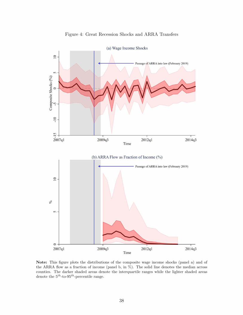
Figure 4: Great Recession Shocks and ARRA Transfers

Note: This figure plots the distributions of the composite wage income shocks (panel a) and ofthe ARRA flow as a fraction of income (panel b, in %). The solid line denotes the median acrosscounties. The darker shaded areas denote the interquartile ranges while the lighter shaded areasdenote the 5th-to-95th-percentile range.

38

Figure 5: Sensitivity Analysis: Dropping County One by One

No Capital Counties

0.2

.4.6

.8D

ensi

ty

.99 1 1.01 1.02 1.03Composite Fiscal Offset β (Adjusted relative to Benchmark)


No Capital Counties

0.1

.2.3

.4D

ensi

ty

.98 .99 1 1.01 1.02Common Shock Offset βM (Adjusted relative to Benchmark)


No Capital Counties

0.2

.4.6

.8D

ensi

ty

.99 1 1.01 1.02 1.03Micro Shock Offset βm (Adjusted relative to Benchmark)


Note: We regenerate the baseline fiscal offset result, leaving one county out at a time, and plot thecorresponding distribution of the composite offsets β for aggregate wage, the macro common offsetsβM for private wage, and the micro common offsets βm for public wage across these “leave-one-county-out” samples in Figure 5, adjusted by the corresponding estimates as in Table 3. The redlines denote the estimates without counties with a state capital.

39

Fig

ure

6:Sen

siti

vit

yA

nal

ysi

s:O

ffse

tsby

the

Siz

esof

AR

RA

Tra

nsf

ers

-.3-.2-.10.1Common Offset

$302

$533

$647

$744

$841

$946

$1,0

78$1

,258

$1,6

30A

mou

nt o

f AR

RA

Tra

nsfe

rs p

er C

apita

Pane

l A: P

rivat

e W

age,

Com

mon

Sho

ck

-.2-.10.1.2County-specific Offset

$302

$533

$647

$744

$841

$946

$1,0

78$1

,258

$1,6

30A

mou

nt o

f AR

RA

Tra

nsfe

rs p

er C

apita

Pane

l B: P

rivat

e W

age,

Cou

nty-

spec

ific

Shoc

k

-.2-.10.1.2Common Offset

$302

$533

$647

$744

$841

$946

$1,0

78$1

,258

$1,6

30A

mou

nt o

f AR

RA

Tra

nsfe

rs p

er C

apita

Pane

l C: P

ublic

Wag

e, C

omm

on S

hock

-.6-.4-.20County-specific Offset

$302

$533

$647

$744

$841

$946

$1,0

78$1

,258

$1,6

30A

mou

nt o

f AR

RA

Tra

nsfe

rs p

er C

apita

Pane

l D: P

ublic

Wag

e, C

ount

y-sp

ecifi

c

Blu

e lin

es d

enot

e th

e es

timat

es a

t the

mea

n w

ith b

oth

com

mon

and

cou

nty

shoc

ks fr

om p

rivat

e an

d pu

blic

wag

e in

com

es.

Note

:W

ere

gen

erate

the

com

mon

an

dco

unty

-lev

eloff

sets

,at

diff

eren

tle

vels

ofth

ed

epen

den

tva

riab

les

usi

ng

qu

anti

lere

gres

sion

s,an

dp

lot

the

mac

roco

mm

onoff

setsβM

,an

dth

em

icro

com

mon

offse

tsβm

for

bot

hp

riva

tean

dp

ub

lic

wag

ein

com

es.

Th

ere

gres

sion

equ

ati

on

isTi,L

=α

+βPrivate

M(λ

iεL−1)

+βPrivate

mε i

,L−1

+βPublic

M(λ

iεL−1)

+βPublic

mε i

,L−1

+ν i.

Th

ed

otte

dli

ne

isth

eze

roli

ne.

.

40

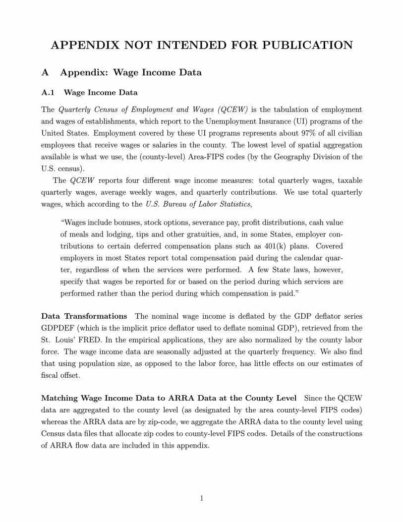
APPENDIX NOT INTENDED FOR PUBLICATION

A Appendix: Wage Income Data

A.1 Wage Income Data

The Quarterly Census of Employment and Wages (QCEW) is the tabulation of employment

and wages of establishments, which report to the Unemployment Insurance (UI) programs of the

United States. Employment covered by these UI programs represents about 97% of all civilian

employees that receive wages or salaries in the county. The lowest level of spatial aggregation

available is what we use, the (county-level) Area-FIPS codes (by the Geography Division of the

U.S. census).

The QCEW reports four different wage income measures: total quarterly wages, taxable

quarterly wages, average weekly wages, and quarterly contributions. We use total quarterly

wages, which according to the U.S. Bureau of Labor Statistics,

“Wages include bonuses, stock options, severance pay, profit distributions, cash value

of meals and lodging, tips and other gratuities, and, in some States, employer con-

tributions to certain deferred compensation plans such as 401(k) plans. Covered

employers in most States report total compensation paid during the calendar quar-

ter, regardless of when the services were performed. A few State laws, however,

specify that wages be reported for or based on the period during which services are

performed rather than the period during which compensation is paid.”

Data Transformations The nominal wage income is deflated by the GDP deflator series

GDPDEF (which is the implicit price deflator used to deflate nominal GDP), retrieved from the

St. Louis’ FRED. In the empirical applications, they are also normalized by the county labor

force. The wage income data are seasonally adjusted at the quarterly frequency. We also find

that using population size, as opposed to the labor force, has little effects on our estimates of

fiscal offset.

Matching Wage Income Data to ARRA Data at the County Level Since the QCEW

data are aggregated to the county level (as designated by the area county-level FIPS codes)

whereas the ARRA data are by zip-code, we aggregate the ARRA data to the county level using

Census data files that allocate zip codes to county-level FIPS codes. Details of the constructions

of ARRA flow data are included in this appendix.

1

B Appendix: Construction of ARRA Flow

The data on ARRA flow were constructed from 18 separate datasets, each of which contains

information taken from reports filed by ARRA grant recipient as required by section 1512 of the

American Recovery and Reinvestment Act of 2009 and as outlined by memorandum M-09-21.

Each of these datasets contains information on the filings from a single quarter. The first period

for which records are available is the third quarter of 2009, and the last data set provided by

Recovery.gov is for the third quarter of 2013.

B.1 Raw Data

The raw data originally obtained from Recovery.gov contain 96 variables, but for the purpose of

constructing a flow variable for each location, only a small subset of these variables is necessary.

The items needed to construct a flow with this dataset are a locator that uniquely identifies

the award or sub-award, an indicator of the recipient role, a dollar amount indicating award

payments, and one or more variables that indicate the location of the disbursements. This

section shall detail the rationale for our choices of variables used in the construction of the

ARRA flow.

B.1.1 Structure of the Data: Recipients

The dataset is hierarchical with observations at the level of prime recipient, sub-recipient, and

vendor. Grants are awarded by federal agencies to prime recipients who record their own ex-

penditure as it progresses, but prime recipients may further delegate funds to sub-recipients

who also record their expenditure or have the prime recipient record their expenditure on their

behalf. There is a further level of recordings representing expenditures on vendors greater than

$25,000. For the purposes of developing a location-specific flow, these vendor observations are

intractable due to their lack of unique identifiers. Because most measures of expenditure for the

prime recipient include that expenditure carried out by the sub-recipient, sub-recipient records

need to be treated in a way that is fundamentally different from prime recipient records; the

recipient role variable is essential in order to maintain the dataset’s hierarchy and avoid double

counting.

B.1.2 Award Identifiers

The award key and the sub-award number are used to identify the awards across time. The

award key is a better identifier than the award number due to a few fundamental flaws in the

award numbers construction.

2

Figure B.1: Award Hierarchy

1. Award numbers were assigned by the awarding or funding agency, but each agency has a

different methodology for creating award numbers. This results in several thousand cases

where award keys that are the same despite their refer to entirely separate grants.

2. Award numbers that refer to the same project change over time when the agency in charge

of award administration is changed.

3. The award numbers are often highly complex (e.g. they are case sensitive and full of special

character) and they often have recording errors as a result.

After the federal government aggregated the reporting data and discovered these issues,

award keys were added to ease the identification of awards before dissemination of the data.

Along with the award key, the sub-award numbers are used. The award key uniquely identifies

the prime recipient grant, but a further piece of information is required to identify sub-recipient

grants. Here, the sub-award number in conjunction with the award key uniquely identifies the

sub-recipient. The same ambiguity does not attend the use of the sub-award number as does the

award number because, by nature of the hierarchy, all sub-awards corresponding to each award

key are assigned sub-award numbers by the same agency.

B.2 Measures of Expenditure

There are several different measures of dollar amounts that could be used to create a flow, but the

most valid and useful is total federal ARRA expenditure, which we shall refer to as expenditure.

3

This measure is the cumulative flow of expenditure to the awardee up to the quarter in question,

but due to the hierarchy of awards and to associate expenditure with locations, it is necessary

to treat this expenditure measure slightly differently for prime and sub-awardees.15

B.3 Data Correction

The first step gone through in correcting the data was removing the duplicate values. There are

a very small number of instances where the award key for the prime recipient is recorded more

than once in the same period. This occurs only in 114 of over a million observations. These are

generally due to small errors in the reporting of the award number leading to duplicated reports.

In these cases, the observation with the lower row number is taken. The same procedure is

carried out on the sub-awards which have a similarly small number of duplicated dates, award

key, sub-award number combinations.

Only one observation was conclusively found to have expenditure misreported. This is the

2013:Q1 observation of award key 102,760 (row 4,262,984). Here, expenditure values should be

recorded as 5 million rather than 5 billion. To account for such misreporting, we remove per

capita transfers that are larger than the 99th percentile of observations. It seems likely that there

are other far smaller errors in the data but these prove very difficult to conclusively identify.

One issue of misreporting that may be correctable in the future but was not carried out here

was those cases in which toward the end of the recording period, expenditure is set at zero once

the project is complete. These were not corrected here because it is difficult to impossible to

systematically distinguish these errors from those cases where awards were revoked.

B.4 Construction of exclusive expenditure

Vendor transactions are not uniquely identifiable due to missing names, missing duns numbers,

and cases of an awardee having a changing number of recorded transactions with the same vendor

15) Of the other possible choices that we considered, the award amount variable is insufficient because it onlycovers prime recipient amounts. Using this would leave something to be desired because it would not track themoney well to where it ends up. After all, the location of sub-recipients may differ markedly from the locationof prime recipients. The local amount variable is also flawed as an account of expenditure; this variable wasconstructed after the fact to aid in the identification of the final location of expenditure. It was calculatedthrough subtracting the sub-award amounts and vendor expenditure of different locations from the prime awardamount. Due to the focus on award amounts rather than money as it is used up over time, for the purposes oftracking spending the local amount is insufficient. More problematically, only those expenditures with a reportin a given period are subtracted from the prime recipient award. Why this is an issue is best explained throughan example. In the first recorded quarter, a university is awarded a one-million-dollar grant. During this quarter,they do not spend any money or engage in any sub-awards, so their local amount variable is one million. A fewquarters later, after the university has expended the money on ongoing transactions with vendors in differentstates and sub-awardees in different counties, the local amount will be one million minus these vendors andsub-award amounts. Finally, in the last period, because these transactions with sub-recipients and vendors havecome to completion, the dataset for that period does not contain a record of these transactions and the localamount for the university returns to one million.

4

over time. This makes vendor transactions nearly impossible properly to track over time, so the

first step in constructing a measure of expenditure that tracks the spending as close to its final

location as possible is to remove all observations where the recipient role is vendor.

A new variable of expenditure (“exclusive expenditure”) now needs to be constructed that

is devoid of double counting. This variable captures expenditure of the awardee, excluding that

expenditure which occurred in a different location. Exclusive expenditure for the prime recipient

must be calculated as the sum of sub-recipient expenditures subtracted from the prime recipient

expenditure for each period. The exclusive expenditure for the sub awardees is then just their

expenditure as marked. In the case where the sum of sub-award amounts exceeds the prime

award amount, the prime award amount is set to zero and the sub-award amounts are taken as-

is. Before this process can be carried out, because our expenditure variable is a cumulative flow,

certain parts of the dataset need to be extended to fill those periods in which no expenditure

report was filed.

Sometimes a record of grant expenditure for an awardee has gaps in time. Filling in these

gaps can be done in a few ways, but to avoid spurious extrapolation, the method chosen here is

to assume that the flow that occurred during the quarter in which the recipient failed to file a

report is zero and set the cumulative expenditure amount of any period following a missing value

equal to the closest expenditure amount before the gap. A similar issue occurs when an award is

complete and the awardee permanently stops filing reports. In this case, a similar assumption of

zero flow is made for further periods, and new rows are populated with new periods. Although

it is not strictly necessary, we ensure that each uniquely identifiable prime and sub-award has

a single observation of the cumulative expenditure in every period to minimize errors in the

construction of the variable.

B.5 Location Identifiers: Assigning FIPS Codes

The dataset does not contain indicators of which county the expenditure occurred in, so county

FIPS codes need to be extrapolated from other data on the location, namely the state, the zip

code, and the city name. Grants that go to US territories and countries outside the US are

removed.

The place of purpose postal code in the raw data identifies the location of the grant with

a ZIP+4 code. Although these codes are extremely precise, identifying a location down to the

city block, ZIP+4 codes are based on postal routes and change monthly. Additionally, data on

ZIP+4 codes is generally unavailable. For this reason, the far more stable five-digit ZIP code

is derived from the ZIP+4. To supplement this method of FIPS county code identification, the

place of purpose city names are also used after cleaning. The reason these ZIP codes must be

supplemented with additional information is that about a quarter of all ZIP codes cross county

boundaries. Town and city names with their associated state cannot be used on their own

5

because many cities and towns also overlap county boundaries.

Two data-sets were used to identify FIPS codes. A combination of HUD and Census data

is used to identify which FIPS code(s) correspond to each ZIP code, and Census data is used

to identify which FIPS code(s) correspond to each city and town name. After joining these two

datasets with the expenditure data, a few steps can be taken to cut down on ambiguity. First,

any observation with only a single FIPS code associated with its zip code or only a single FIPS

code associated with its city name is assigned that FIPS code. Second, ambiguity can be further

attenuated through taking those cases where both ZIP code and city name exhibit ambiguity

and taking those instances where only one of the possible FIPS codes associated with the ZIP

and city match. In this case, the matching FIPS code is assigned. Using both ZIP codes and

city names cuts the incidence of having one or more possible counties from 26% to 6% of all

observations.

This 6% of observations require that the expenditure be distributed in some fashion, but

one further step can be made to increase the accuracy of this distribution. Through keeping

only those FIPS codes where both the possible city FIPS and the possible ZIP-FIPS match

each other, the number of possible choices can often be down substantially. With the remaining

possible county codes, the expenditure amounts are split amongst the counties in proportion

with each possible county’s population.

B.6 Finishing Up

Retrieving each county’s expenditure requires summing up the distributed exclusive expenditure

values associated with each county FIPS code in each period. To derive the flow, take the first

difference of these values. It is important to note that because data reporting started in Q3

of 2009 but actual disbursements of ARRA expenditure started earlier in the second quarter of

2009. This flow variable is then transformed into per capita real terms in the same fashion as

the wage income variable.

C Appendix: Additional Tables and Figures

6

Figure C.2: Kernel densities of key estimated parameters - Aggregate Wage

01

23

4D

ensi

ty

.2 .4 .6 .8 1ρi

0.2

.4.6

.8D

ensi

ty

-1 0 1 2 3λi

010

2030

40D

ensi

ty

0 .05 .1 .15 .2σε

it

Note: This figure plots the kernel density distribution of estimates of selected parameters across allcounties i. σε

i denotes the standard deviation of the income innovation εit over time for county i.

7

Figure C.3: Estimated parameters - Private and Public

Private Public

01

23

4D

ensi

ty

.2 .4 .6 .8 1ρi

01

23

Den

sity

.2 .4 .6 .8 1ρi

0.2

.4.6

.8D

ensi

ty

-1 0 1 2 3λi

0.2

.4.6

.8D

ensi

ty

-1 0 1 2 3λi

010

2030

Den

sity

0 .05 .1 .15 .2σε

it

010

2030

Den

sity

0 .05 .1 .15 .2σε

it

Note: This figure plots the kernel density distribution of estimates of selected parameters across allcounties i. σε

i denotes the standard deviation of the income innovation εit over time for county i.

8

Table A1: Moments of Shocks

(a) Standard Deviation

Sample: Great Recession 2007:Q4-2009:Q2 Aggregate Private PublicMacro Shocks (λiεt) 0.018 0.019 0.017Micro Shocks (εit) 0.055 0.083 0.056Composite Shocks (λiεt + εit) 0.059 0.085 0.058Common Shocks (εt) without County Loadings (λi) 0.017 0.018 0.005

Full-sample: 1990Q1-2018Q4Macro Shocks (λiεt) 0.015 0.017 0.012Micro Shocks (εit) 0.055 0.085 0.061Composite Shocks (λiεt + εit) 0.057 0.087 0.062Common Shocks (εt) without County Loadings (λi) 0.013 0.014 0.009

(b) Cumulative Great Recession Shocks: First Moment

Sample: Great Recession 2007:Q4-2009:Q2 Aggregate Private PublicMacro Shocks (λiεt) -0.046 -0.088 0.028Micro Shocks (εit) -0.003 0.005 0.024Composite Shocks (λiεt + εit) -0.049 -0.083 0.053Common Shocks (εt) without County Loadings (λi) -0.046 -0.089 0.030

9

Figure C.4: Estimated Shocks to Private and Public County Wage Income

-.1

-.05

0

.05

.1

λ iε t

+ ε it

2005q1 2008q1 2011q1 2014q1

Private Wage Income

-.1

-.05

0

.05

.1

λ iε t

+ ε it

2005q1 2008q1 2011q1 2014q1

Public Wage Income

-.04

-.02

0

.02

.04

λ iε t

2005q1 2008q1 2011q1 2014q1

-.04

-.02

0

.02

.04λ i

ε t

2005q1 2008q1 2011q1 2014q1

-.1

-.05

0

.05

.1

ε it

2005q1 2008q1 2011q1 2014q1Time

-.1

-.05

0

.05

.1

ε it

2005q1 2008q1 2011q1 2014q1Time

The blue lines denote ARRA Passage (2009 February).

10

did the american recovery and reinvestment act help

Documents