did the pursuit of good schools contribute to the u.s ... the pursuit of good schools contribute to...

1

Did the Pursuit of Good Schools Contribute to the U.S. Housing Bubble?

Michael Insler†

U. S. Naval Academy, Department of Economics, 589 McNair Rd, Annapolis, MD 21402

Phone: 410-293-6881, Email: [email protected]

Kurtis Swope

U. S. Naval Academy, Department of Economics, 589 McNair Rd, Annapolis, MD 21402

Phone: 410-293-6892, Email: [email protected]

August 13, 2013

Abstract: Using data from the American Housing Survey 2001-2009, we find that households’

expenditures for homes in neighborhoods with self-identified “good schools” and the resulting

mortgage-to-income ratios for such households rose during the key bubble period relative to the

periods before and after the bubble. This pattern persists after conditioning on a variety of

household, demographic, and socioeconomic controls. Most notably, difference in differences

models and propensity score matching techniques provide evidence that the pursuit of good

schools contributed to the housing bubble. (R21, I24, G01)

Keywords: Residential choice; housing expenditures; school quality; U.S. housing crisis

†Corresponding author

mailto:[email protected]

mailto:[email protected]

2

1. INTRODUCTION

In the U.S., access to a particular public school is typically linked directly to residential

location, with each home address assigned to one public elementary school, middle schoo1, and

high school. According to the U.S. Department of Education (2009), around 90 percent of K-12

students attend public schools, with 75 percent attending an “assigned” school and 15 percent

attending a “chosen” public school. For families with school-aged or younger children, the

quality of the schools in a neighborhood, therefore, plays an important role in the choice of a

neighborhood and home and, in some cases, is the primary factor. However, given the variation

in school quality across neighboring districts, and given the scarcity of homes within a district,

homebuyers seeking access to the best public school systems generally pay a significant

premium to live in such districts (over $200,000 more, on average, in the 100 largest U.S.

metropolitan areas, according to Rothwell (2012)). This may be because the value of a good

public school system is capitalized into the value of homes in the district, and because homes in

the best districts are typically larger and of higher quality (Rothwell, 2012). Affordable rental

housing in such districts may also be limited by scarcity and exclusionary zoning practices

(Rothwell, 2012) that are intended to limit the construction of multi-family dwellings.

Furthermore, good public schools are often in “high-opportunity” neighborhoods (McClure,

2010) and accompanied by other local public good amenities, such as lower crime, better

shopping, more parks and recreation facilities, and greater employment opportunities that further

contribute to higher home prices in the area.

A large literature focuses on estimating willingness-to-pay for school quality using

hedonic estimation techniques to capture how much school quality is capitalized into the value of

a home. However, estimating the demand for good schools alone is complicated if

3

neighborhoods with good schools tend to have other local public good amenities. When samples

are restricted to only houses located near district attendance boundaries, estimates of willingness-

to-pay for school quality, though significant, are one-half (Black, 1999) to one-quarter (Kane et

al., 2006) as large as with the unrestricted samples. Alternative approaches to measuring

willingness-to-pay for school quality include analyzing changes in home values following the

publication of new information on school quality (Figlio and Lucas, 2004; Fiva and Kirkenboem,

2008), or following policy changes, such as the adoption of school choice programs (Rebak,

2005). Results from these approaches consistently indicate a positive and significant willingness-

to-pay for access to good public schools.

However, because of the strong link between residential location and public schools,

homebuyers must nevertheless purchase a bundle of neighborhood characteristics and cannot

easily isolate the “good schools” feature of a neighborhood from other characteristics. The

effective cost to access high-quality schools, therefore, may be significantly higher than the

estimated willingness-to-pay for better schools alone found by Black (1999) and others. Low and

moderate-income households, therefore, generally have fewer schooling options than high-

income households. High-income households have the means to afford homes near high-scoring

public schools, or they can choose private schools when public school options are not

satisfactory. Low-income households, to the extent that they have a choice, must choose between

living in low-scoring school districts where home prices are lower or affordable rental housing is

available, or allocating a substantial portion of their budgets to housing simply to access quality

public schools. Even with programs such as the Federal Housing Choice Voucher (HVC)

program aimed at assisting low-income residents in moving to high-opportunity neighborhoods,

4

few participating households are able to find rental units in better neighborhoods because of a

scarcity of supply and because of competition from unsubsidized households (McClure, 2010).

It would not be surprising, therefore, that given a limited window of opportunity to

purchase a home in a better school district, many households of various income levels might take

advantage of the opportunity even if it meant purchasing more home (and having a larger

mortgage) than they might otherwise have chosen. We hypothesize that rising home prices and

lax borrowing constraints during the early years of the recent U.S. housing bubble may have

afforded such a perceived opportunity. School quality is relative, and each household’s

perception of a “good school” may depend on the quality of the school they currently have

access to relative to other schools on the performance ladder. Households may have viewed

rising home prices and unusually low mortgage interest rates as an opportunity to purchase an

otherwise “unaffordable” home in a better neighborhood with better schools. The U.S. housing

bubble and subsequent financial crisis and recession had significant and lasting consequences for

homebuyers and the U.S. economy. Did the pursuit of good schools contribute to the housing the

bubble, as we hypothesize? That is, did the link between residential location and school access

provide a vehicle through which homebuyers seeking good schools fueled the already-expanding

bubble by taking advantage of a limited opportunity to access better neighborhoods with better

schools?

In this paper we use data from the American Housing Survey (AHS) 2001-2009 to

characterize the pattern of housing expenditures across households and across time periods.

Figure B.1, which shows the seasonally-adjusted U.S. housing price index since 1990, illustrates

the housing price bubble. Though when, exactly, the “bubble” began is a matter of some

speculation, for purposes of our analysis, we define the “pre-bubble” period as 2000-2002, the

5

“bubble” period as 2003-2006, and the “post-bubble” period as 2007-2009. We should note that

our main results are robust to reasonable alternate year groupings for the pre-bubble, bubble, and

post-bubble periods. The AHS survey data provide information on the purchase price of the

home, size of the homeowner’s mortgage, and characteristics of the home, the homeowner, the

household, and the neighborhood. Importantly, the data also provide information on why the

homeowner chose the neighborhood and home, including whether “good schools” was the

primary reason. Therefore, we can identify the extent to which housing expenditures, measured

by both home prices and resulting mortgage-to-income ratios, were influenced by the pursuit of

good schools, conditional on income, demographics, and other factors. We compare the patterns

of home expenditures across households during the critical years of the U.S. housing boom and

bust.

We find that the pursuit of high quality schools played a significant role in the housing

boom. Households whose primary reason for choosing a neighborhood was “good schools”

demonstrated a higher willingness-to-pay for a home than comparable households who chose a

neighborhood for other reasons, and the difference was largest during the key “bubble” period.

We investigate this finding using a series of empirical techniques. Estimates from basic OLS

regressions show that, holding a wide range of observable factors constant (housing unit,

neighborhood, and the householders’ characteristics), the strength of correlation between demand

for school quality and housing expenditures grew to a peak during the critical boom years 2003-

2006, and then vanished in the following years. Furthermore, mortgage-to-income ratios follow a

similar pattern relative to the “good schools” cohort during the “bubble” period. Using difference

in differences models and propensity score matching techniques, we extend these findings, under

reasonable identification assumptions, to argue that the pursuit of good schools acted on

6

homebuyers’ willingness-to-pay particularly strongly during the height of the housing boom. We

view the causal link as an artifact of the low interest rates and rising home prices (which

functioned as proxies for higher income) at the height of the housing boom, in effect boosting the

usual premium paid by homebuyers seeking to reside in neighborhoods with high quality

schools.

While it is difficult to compare our estimates of willingness-to-pay for “good schools” to

those calculated by Black (1999) and others because our data lacks more objective measures of

school quality, our estimates are reasonable in magnitude and consistent across various empirical

strategies. Holding all other observable characteristics constant, we find that households who

chose their neighborhood primarily to access high quality schools paid roughly 11.5 percent

more at the bubble’s height (2003-2006), compared to those who chose their neighborhood for

other primary reasons before and during the bubble. For the median bubble-era homebuyer who

favored “good schools,” this equates to, on average, a $26,000 premium.

The remainder of the paper proceeds as follows. Section 2 provides background on

research examining the link between school quality, housing expenditures, and residential

choice. Section 3 discusses the data, followed by the empirical methods, results, and discussion

in Section 4. Section 5 provides concluding remarks.

2. RESIDENTIAL CHOICE AND SCHOOL QUALITY

Explanations for the recent U.S. housing market bubble, collapse, and resulting financial

crisis include speculative and “irrationally exuberant” borrowers,1 predatory lending practices,

2

1 Shiller (2000).

2 Center for Responsible Lending (2009); Financial Crisis Inquiry Commission (2010).

7

excessive risk-taking by investment banks,3 unsustainable global financial imbalances,

4

favorable treatment of capital gains from real estate,5 prolonged expansionary monetary policy,

6

financial-sector deregulation,7 rapid and inadequately-regulated financial innovation,

8 and

government initiatives to increase home ownership rates among lower-income households.9

Nearly all of these explanations ascribe a central role to the sub-prime mortgage market both in

generating the housing price bubble and subsequently precipitating the housing market collapse.

Often ignored, however, is the fact that the vast majority of homebuyers, whether they are prime

or sub-prime borrowers, or high, middle, or low-income families, simply choose to purchase a

home in hopes of improving their well-being. And it takes buyers willing to pay increasing prices

for homes to fuel a housing market bubble.

Buying a home brings many benefits including pride of ownership, access to a

neighborhood and its amenities, and financial advantages from tax incentives and the building of

equity. For families with children or who plan to have children, home location in the U.S. also

determines access to most public schools. Rental housing, particularly affordable, multi-family

dwellings, is often restricted or limited in neighborhoods with the highest-performing public

schools (Rothwell, 2012), making a home purchase often the most direct, and perhaps only, way

3 Stiglitz (2011).

4 Obstfeld and Rogoff (2007).

5 Smith (2007); Gjerstad and Smith (2011). For example, the 1997 Taxpayer Relief Act exempted from taxation

housing capital gains (up to $500,000). 6 Taylor (2011).

7 Stiglitz (2011).

8 Miele (2011).

9 Roberts (2010); Wallison (2011). For example, the Community Reinvestment Act of 1977 (and subsequent

amendments) and the 1992 Affordable Housing Goals (AHG) initiative led to lower lending standards and increased

the role of the Government-Sponsored Enterprises (GSEs) Fannie Mae and Freddie Mac in backing residential

mortgage debt.

8

to access high quality schools.10

Open enrollment and intra-district school choice programs, such

as the San Francisco Unified School District, are relatively uncommon.11

Stratification of households across districts that vary in the quality of public schools and

other public services and amenities is formally explained by the well-known Tiebout (1956)

model in public finance. According to the standard model, communities offer a basket of public

goods and services and an attendant tax level necessary to finance the provision of public goods.

Households (assuming a reasonable level of household mobility) sort themselves across

jurisdictions based on their preferences for public goods and their ability to pay the associated

taxes in a community. An equilibrium in the model consists of set of communities, tax and public

good levels, and household composition such that each community collects sufficient taxes to

finance the public good level in the community, and no household can unilaterally increase its

welfare by moving to a different community. Based strictly on the Tiebout model and the strong

link between residential location and public school access in the U.S., we would expect lower-

income households to live in communities with lower taxes, lower local expenditures on

education, and lower-quality schools.

Supplemental state and federal funding of public schools can provide a more equitable

allocation of funding resources across schools relative to what would occur under pure local

financing. According to the U.S. Department of Education (2005), 46.9 percent of public K-12

education funding for the 2004-2005 academic year came from state governments, while 44

10

Households may be able to access schools, in some cases, without necessarily living in the district by obtaining a

limited number of waivers to attend an out-of-district school, or by illegally using a fraudulent mailing address or

the address of a relative who lives in the district. Residency verification and the degree of enforcement vary

significantly across school districts. Some schools may “turn a blind eye” while others will hire private residency

verification contractors to enforce residency requirements. 11

According to the U.S. Department of Education (2009), 16 percent of students in 2007 were attending a “chosen”

public school (defined as any school other than the one they were assigned to), which could include waivers, charter

schools, or school choice programs.

9

percent came from local governments. Federal government financing amounted to 9.2 percent.

However, evidence on the link between levels of per pupil expenditures and student performance

is mixed and controversial (for example, see Hanushek, 1996). While a thorough review of the

large literature on this issue is not within the scope or purpose of our analysis, it is sufficient to

note that households’ perceptions of the quality of a particular school are driven by more than

per pupil expenditures alone. Indeed, common perceptions of “school quality” are often driven

by student learning outcomes (such as performance on standardized tests, and graduation and

college attendance rates), although the U.S. Department of Education (2000) cites 13 “indicators

of school quality” that affect student learning, many of which (such as teacher experience, class

size, and available technology) may be closely linked with financial resources and expenditures

per pupil.

Empirical evidence generally confirms the importance of school quality for homebuyers.

A rich literature has estimated the value of good schools through various hedonic methods

measuring the capitalization of school quality into house prices. The principle concern of these

studies is isolating the value of good schools from other local services and amenities. For

example, Bogart and Cromwell (1997) use an overlapping jurisdictions approach using homes

that are in the same municipal jurisdictions and, therefore, should have common local

government services, but are associated with different school districts. Black (1999)

demonstrates that when samples are restricted to houses that lie very near to school boundaries

and, therefore, are very likely in the same “neighborhood” but associated with different school

districts, the estimated value of school quality is about half of that obtained with a standard,

unrestricted hedonic sample. Alternatively, based on a unique dataset of residential choice

decisions in the Columbus, Ohio area, Bayoh, et al. (2006) find that neighborhood public school

10

quality has the single largest effect on the probability of a household choosing a particular

neighborhood.

In this paper we take an alternative approach. Our analysis focuses on whether the pursuit

of quality schools played a role in fueling the U.S. housing bubble, and whether there was any

significant change in the relationship between housing choices and school quality during the

bubble period relative to the years around it. Our hypothesis is that low interest rates and rising

home prices—which were particularly prominent during the bubble—acted as proxies for higher

income, thereby leading households with a preference for “good schools” to increase their

willingness-to-pay for homes in neighborhoods with quality schools by more than they would

have without the “bubble-propagated” influence. The “good schools” effect that we seek to

uncover stems from the strong link between residential location and public school access, and the

relative scarcity of homes in districts with the best schools. Our analysis is unique in that our

data represent a cross section of home purchases across the nation and across time, and we are

able to examine the pattern of home purchases before, during, and after the housing bubble,

controlling for both characteristics of the household and home location. While the data do not

yield specific information about the exact quality of schools in a particular neighborhood, as

measured, for example, by student scores on standardized tests or other attributes of the

individual schools, we do have information about homebuyers’ perceptions of the quality of the

schools and how important school quality was in their purchase decision. And it is homebuyers’

perception of quality that ultimately determines their willingness-to-pay when school quality is

an important consideration.

11

3. DATA AND EMPIRICAL OBSERVATIONS

3.1 American Housing Survey

For the empirical analysis, we use microdata from the American Housing Survey (AHS),

a longitudinal survey that addresses the quality of housing in the United States. In a joint effort

with the U.S. Census Bureau, the U.S. Department of Housing and Urban Development collects

AHS data every other year. The sampled objects are specific housing units, regardless of changes

in ownership or residency that may occur between survey periods (although we observe such

changes). Housing units participating in the AHS represent a cross section of all housing in the

nation. The survey provides sampling weights; each housing unit in the sample represents about

2,000 housing units in the United States.

The construction of our sample is as follows. The unrestricted AHS sample contains

341,145 observations of housing units, taken from 85,913 unique housing units across five

biennial survey waves from 2001-2009. We limit the sample to housing units classified as

“house, apartment, or flat” and to those never listed as part of a condominium or cooperative. We

also omit units that are (at any point in the sampling period) owned by a public housing authority

or listed with a value less than $15,000. This reduces the number of observations to 266,674

(68,031 unique housing units). Since we aim to study the connection between residential choice

and schooling—a choice made at the time of the home purchase—our sampling objects of

interest consist of observations of housing purchases. In other words, although we may observe

each housing unit several times throughout the panel, we use only the first observation that

follows the purchase of a unit.12

As such, we restrict the sample to the initial observations of

12

Some housing units may change hands more than once within the panel, in which case we take multiple

observations from that unit.

12

units purchased or constructed during the survey period from 2000-2009 13

(46,377 observations

from 29,283 unique housing units). In order to examine the subpopulation whose housing-

purchase decisions reflect the needs of school-aged children, we omit residencies that contain

more than one family, units that are not owner-occupied or purchased without a mortgage, units

that are designated for “vacation or other short term use,” and units in which both the

householder and spouse (if present) are over age 60 (leaving 9,340 observations from 8,383

unique housing units). Lastly, we omit observations with missing values for crucial variables

such as income, purchase price, or neighborhood choice preferences, giving us a final sample

size of 6,475 observations of home purchases from 5,991 unique housing units. Although this

number may appear small in comparison to size of the unrestricted sample, it is important to note

that it represents only the population of suitable housing purchases occurring from 2000-2009.

As each sampling unit in the AHS represents about 2,000 housing units in the U.S. as a whole,

our final sample is representative of nearly 13 million housing transactions from that time span.

3.2 Descriptive Statistics

Table A.1 contains summary statistics for our restricted AHS sample of 6,475 households

who purchased homes from 2000-2009. Relative to the U.S. population, our sample of

homebuyers is disproportionately white, married, and has at least some level of college education

or above. The average number of children per home is 1.3. The median household income in our

sample ($75,000) is notably lower than the mean ($95,315). Importantly, respondents to the AHS

survey are asked about their main reason for choosing a neighborhood (with options given

towards the bottom of Table A.1), and 11 percent of our respondents chose “good schools” as the

13

Although the AHS has existed since 1973, it received a major overhaul in 1997. Our sample includes housing

units purchased during the years 2000-2009 (i.e. over five waves of survey data: 2001, 2003, 2005, 2007, 2009) in

13

primary reason.14

Conditional averages (not shown in the table) indicate that this proportion was

only slightly higher during the “bubble” years—12.4 percent during 2003-2006—compared to

12.1 percent during the preceding three years. Other popular primary reasons for neighborhood

choice include the specific housing unit, work-related convenience, and the aesthetics of the

neighborhood. Table A.1 indicates that those whose primary reason for purchasing a home was

“good schools” tended to have higher family income ($103,648 versus $94,234) and more

children (1.83 versus 1.23) compared to those who purchased a home for other reasons during

this time period, but otherwise the two cohorts of homebuyers are comparable. Notably, the

“good schools” cohort spent roughly $46,000 more, on average, to buy a home.

Our objective is to characterize the pattern of housing expenditure decisions before,

during, and after the U.S. housing bubble, particularly as it relates to the pursuit of high quality

schools. Figures B.2.1 and B.2.2 provide the mean purchase price of a home (with 95 percent

confidence intervals) by year of purchase; the two plots separate families whose primary reason

for choosing a neighborhood was “good schools” and those whose primary reason was one of the

other options. The comparison is striking. Rising mean purchase prices reflect the general

housing bubble that occurred over this period. However, while mean home purchase prices for

the “good schools” cohort were just marginally higher during 2000 and 2001, mean home

purchase prices for this group rose sooner, greater, and faster, and peaked in 2006. Furthermore,

there was a considerably greater crash in purchase prices for the “good schools” cohort in the

bust year of 2007 that corresponded with the acceleration of the subprime mortgage crisis. An

additional exercise is to examine the degree of leveraging attributable to school quality concerns

order to focus on such decisions made shortly before, during, and after the housing price bubble in the United States. 14

According to the U.S. Department of Education (2009), the parents of 27 percent of public school students

indicated that they had moved to their current neighborhood so that their children could attend that school, but this

does not imply that schools were the “primary reason” for all such households.

14

by plotting mortgage size rather than house price. Figures B.3.1 and B.3.2 compare the

mortgage-to-income ratios across the two cohorts. While the confidence intervals are large, a

consistent pattern remains: Households who moved for “good schools” borrowed more relative

to income nearly every year from 2000-2009, with the greatest differences occurring in the years

2004 and 2005.

3.3 Ordinary Least Squares (OLS)

While compelling, the figures alone do not substantiate the claim that the pursuit of high

quality public schools played a significant role in the U.S. housing bubble. Selection bias could

account for the more dramatic rise in house prices paid by those seeking good schools. We

estimate simple ordinary least squares (OLS) models to check that the patterns in Figure B.2

persist after controlling for selection on observable characteristics.

We consider an OLS specification in which the natural logarithm of purchase price is the

dependent variable and the good schools dummy is the main control variable of interest.15

Thus

this specification is a single difference model, but we estimate it on three separate subsamples

from “pre-bubble” years (home purchases made during 2000-2002), “bubble” (2003-2006), and

“bust” (2007-2009).16

We also control for the age, race, gender, and marital status of the

responder, spouse’s age, the education background of the responder and spouse, number of

children in the household, and self-reported neighborhood quality (on a 1-10 scale). The AHS

data indicates the census region (Northeast, Midwest, South, and West) and whether the unit is

15

Recall from Table A.1 that we also observe several other “main reasons for choosing the neighborhood.” These

dummies also enter as covariates, so the reference group for good schools is “other” as the main reason for choosing

the neighborhood. 16

Our qualitative results are robust to reasonable alternative year groupings, such as 2000-2001/2002-2006/2007-

2009 or 2000-2003/2004-2005/2006-2009. Results from these robustness checks are available upon request.

15

part of a metropolitan statistical area (MSA).17

Lastly, we account for time trends in nominal

housing prices (within each purchase year subgroup) by including dummies for the year of the

unit’s purchase.

Table A.2 displays regression results, estimated via OLS, incorporating sampling weights

and heteroscedasticity-robust standard errors. Household income is a principal determinant of

housing expenditures, as expected, with income elasticities ranging from 0.26 to 0.4 in the three

subsamples. For brevity, Table A.2 omits estimates of several of the other household

characteristics’ coefficients.18

We are most interested in the results as they pertain to “good

schools” as the primary reason a household chose a particular neighborhood. Here, the

coefficient on the good schools variable is positive for both the pre-bubble and bubble cohorts,

but significant and nearly four times larger for the latter. The difference vanishes altogether

during the bust period. We interpret our estimates to say that during the pre-bubble years, those

who chose their neighborhood primarily for nearby schools paid on average 5 percent more for

their housing (compared to those who chose their neighborhood for “other” reasons), holding all

observable conditions constant, but they paid nearly 20 percent more during the bubble years.

These results suggest a higher willingness-to-pay as the housing bubble expanded (specifically in

order to access good schools) that is independent of observable trends in the housing market

during the time. While we can expect home prices to be higher, in general, in districts with the

17

The Northeast and MSA central city categories are the reference groups, respectively. MSA categorical variable

options are: MSA central city, MSA urban, MSA rural, no MSA urban, and no MSA rural. A metropolitan statistical

area is a region with high population density at its core and close economic ties throughout the area. Examples of

MSAs include the Washington—Arlington—Alexandria DC-VA-MD-WV MSA, or the Dallas—Fort Worth—

Arlington TX MSA. 18

Of these, older homebuyers tend to purchase more expensive homes, and the coefficient on number of children is

positive for all three cohorts. There is evidence that, relative to white households, black and other minority

households choose lower-priced homes, while Asian households pay more for their homes. In general, households

where the responder and spouse had less than a bachelor’s degree tend to spend less on homes compared to those

with a bachelor’s degree, while those with graduate degrees spend more. Housing in the South and Midwest is

cheaper relative to the Northeast, on average, while the West is more expensive. Housing in an MSA but outside the

city center is more expensive than in the city center, but housing outside an MSA entirely is cheaper.

16

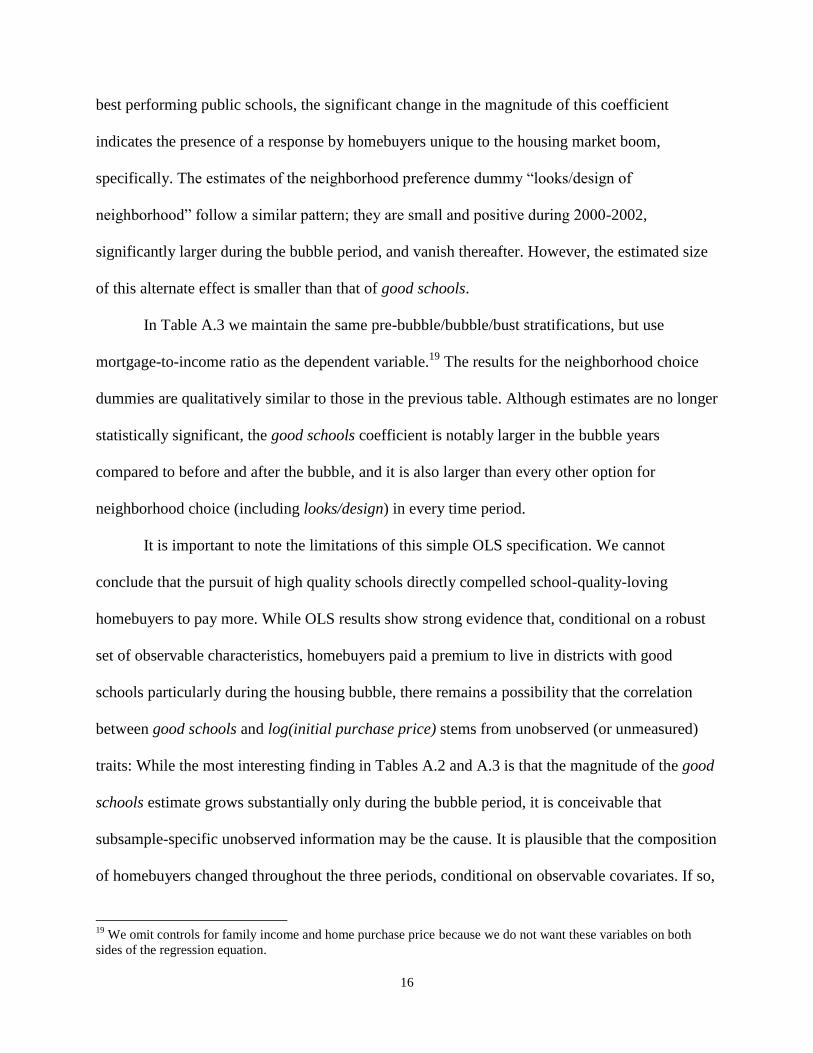
best performing public schools, the significant change in the magnitude of this coefficient

indicates the presence of a response by homebuyers unique to the housing market boom,

specifically. The estimates of the neighborhood preference dummy “looks/design of

neighborhood” follow a similar pattern; they are small and positive during 2000-2002,

significantly larger during the bubble period, and vanish thereafter. However, the estimated size

of this alternate effect is smaller than that of good schools.

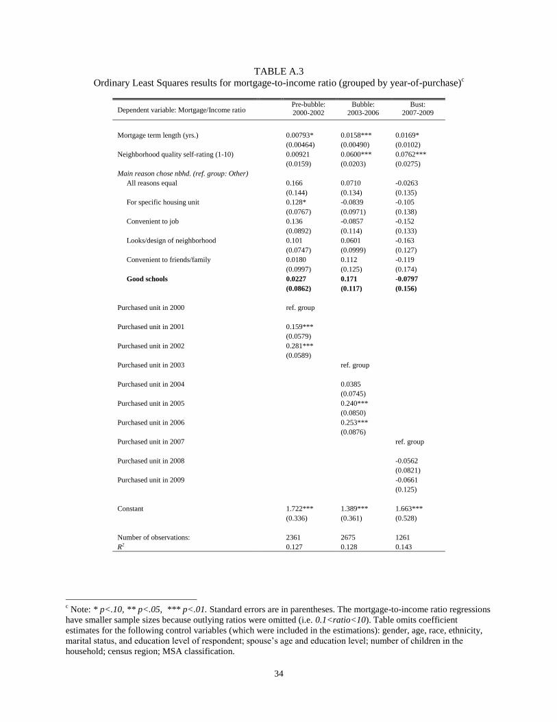
In Table A.3 we maintain the same pre-bubble/bubble/bust stratifications, but use

mortgage-to-income ratio as the dependent variable.19

The results for the neighborhood choice

dummies are qualitatively similar to those in the previous table. Although estimates are no longer

statistically significant, the good schools coefficient is notably larger in the bubble years

compared to before and after the bubble, and it is also larger than every other option for

neighborhood choice (including looks/design) in every time period.

It is important to note the limitations of this simple OLS specification. We cannot

conclude that the pursuit of high quality schools directly compelled school-quality-loving

homebuyers to pay more. While OLS results show strong evidence that, conditional on a robust

set of observable characteristics, homebuyers paid a premium to live in districts with good

schools particularly during the housing bubble, there remains a possibility that the correlation

between good schools and log(initial purchase price) stems from unobserved (or unmeasured)

traits: While the most interesting finding in Tables A.2 and A.3 is that the magnitude of the good

schools estimate grows substantially only during the bubble period, it is conceivable that

subsample-specific unobserved information may be the cause. It is plausible that the composition

of homebuyers changed throughout the three periods, conditional on observable covariates. If so,

19

We omit controls for family income and home purchase price because we do not want these variables on both

sides of the regression equation.

17

the coefficient estimates could reflect differences stemming from distinctly different subgroups

of homebuyers. The next section presents our evidence of a bubble-period-specific effect of the

pursuit of good schools on housing expenditures.

4. THE CASE FOR CAUSALITY

To better address observable characteristics that may influence housing expenditure

decisions, we consider two more empirical approaches. First, we discuss identification and

present estimation of difference in differences (DD) specifications using the entire sample (2000-

2009) of housing purchases. Second, we employ propensity score matching (PSM) algorithms

once again on the three subgroups. Under reasonable assumptions (discussed below) both

approaches yield comparable results: The pursuit of good schools affected housing expenditures

most strongly during the bubble years of 2003-2006. We argue at the end of this section that its

influence was economically significant in the context of the housing boom.

4.1 Identification

In this section, we adopt a somewhat unconventional DD specification, as our

identification strategy is not derived from an exogenous policy change that occurred at a certain

point in time. Instead, we rely on the empirical observations of the previous section to define our

treatment group as homebuyers who selected their neighborhood for “good schools” during the

bubble years. Our time period of interest (2000-2009) permits us to consider two alternate

control groups: 1) homebuyers who did not select their neighborhood for “good schools” before

and during the bubble, and 2) homebuyers who did not select their neighborhood for “good

18

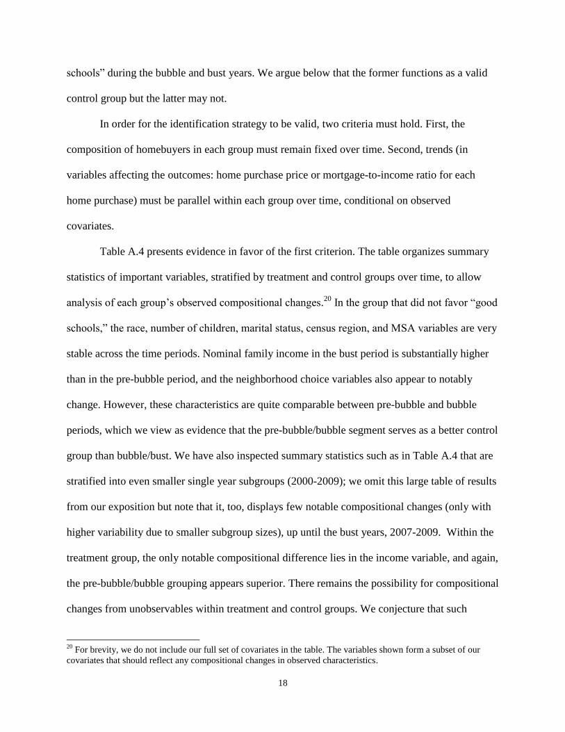
schools” during the bubble and bust years. We argue below that the former functions as a valid

control group but the latter may not.

In order for the identification strategy to be valid, two criteria must hold. First, the

composition of homebuyers in each group must remain fixed over time. Second, trends (in

variables affecting the outcomes: home purchase price or mortgage-to-income ratio for each

home purchase) must be parallel within each group over time, conditional on observed

covariates.

Table A.4 presents evidence in favor of the first criterion. The table organizes summary

statistics of important variables, stratified by treatment and control groups over time, to allow

analysis of each group’s observed compositional changes.20

In the group that did not favor “good

schools,” the race, number of children, marital status, census region, and MSA variables are very

stable across the time periods. Nominal family income in the bust period is substantially higher

than in the pre-bubble period, and the neighborhood choice variables also appear to notably

change. However, these characteristics are quite comparable between pre-bubble and bubble

periods, which we view as evidence that the pre-bubble/bubble segment serves as a better control

group than bubble/bust. We have also inspected summary statistics such as in Table A.4 that are

stratified into even smaller single year subgroups (2000-2009); we omit this large table of results

from our exposition but note that it, too, displays few notable compositional changes (only with

higher variability due to smaller subgroup sizes), up until the bust years, 2007-2009. Within the

treatment group, the only notable compositional difference lies in the income variable, and again,

the pre-bubble/bubble grouping appears superior. There remains the possibility for compositional

changes from unobservables within treatment and control groups. We conjecture that such

20

For brevity, we do not include our full set of covariates in the table. The variables shown form a subset of our

covariates that should reflect any compositional changes in observed characteristics.

19

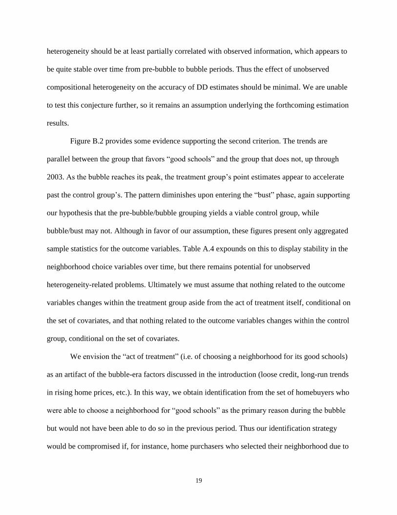
heterogeneity should be at least partially correlated with observed information, which appears to

be quite stable over time from pre-bubble to bubble periods. Thus the effect of unobserved

compositional heterogeneity on the accuracy of DD estimates should be minimal. We are unable

to test this conjecture further, so it remains an assumption underlying the forthcoming estimation

results.

Figure B.2 provides some evidence supporting the second criterion. The trends are

parallel between the group that favors “good schools” and the group that does not, up through

2003. As the bubble reaches its peak, the treatment group’s point estimates appear to accelerate

past the control group’s. The pattern diminishes upon entering the “bust” phase, again supporting

our hypothesis that the pre-bubble/bubble grouping yields a viable control group, while

bubble/bust may not. Although in favor of our assumption, these figures present only aggregated

sample statistics for the outcome variables. Table A.4 expounds on this to display stability in the

neighborhood choice variables over time, but there remains potential for unobserved

heterogeneity-related problems. Ultimately we must assume that nothing related to the outcome

variables changes within the treatment group aside from the act of treatment itself, conditional on

the set of covariates, and that nothing related to the outcome variables changes within the control

group, conditional on the set of covariates.

We envision the “act of treatment” (i.e. of choosing a neighborhood for its good schools)

as an artifact of the bubble-era factors discussed in the introduction (loose credit, long-run trends

in rising home prices, etc.). In this way, we obtain identification from the set of homebuyers who

were able to choose a neighborhood for “good schools” as the primary reason during the bubble

but would not have been able to do so in the previous period. Thus our identification strategy

would be compromised if, for instance, home purchasers who selected their neighborhood due to

20

good schools during the bubble would have selected it for another reason during a different

period. Our intuition as to why school choice played a strong role during the bubble period but

not in others stems from bubble-era financial markets’ loose-money policies towards buyers,

which provided a vehicle through which the pursuit of good schools further inflated the housing

bubble.

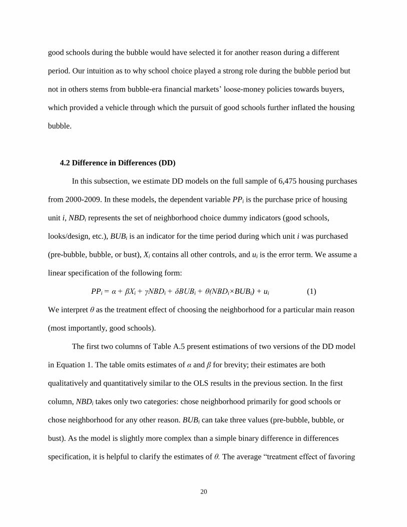
4.2 Difference in Differences (DD)

In this subsection, we estimate DD models on the full sample of 6,475 housing purchases

from 2000-2009. In these models, the dependent variable PPi is the purchase price of housing

unit i, NBDi represents the set of neighborhood choice dummy indicators (good schools,

looks/design, etc.), BUBi is an indicator for the time period during which unit i was purchased

(pre-bubble, bubble, or bust), Xi contains all other controls, and ui is the error term. We assume a

linear specification of the following form:

PPi = α + βXi + γNBDi + δBUBi + θ(NBDi×BUBi) + ui (1)

We interpret θ as the treatment effect of choosing the neighborhood for a particular main reason

(most importantly, good schools).

The first two columns of Table A.5 present estimations of two versions of the DD model

in Equation 1. The table omits estimates of α and β for brevity; their estimates are both

qualitatively and quantitatively similar to the OLS results in the previous section. In the first

column, NBDi takes only two categories: chose neighborhood primarily for good schools or

chose neighborhood for any other reason. BUBi can take three values (pre-bubble, bubble, or

bust). As the model is slightly more complex than a simple binary difference in differences

specification, it is helpful to clarify the estimates of θ. The average “treatment effect of favoring

21

access to good schools” is the premium paid during the bubble period relative to one of the other

two periods. Since only the bubble period estimate of good schools is significant (in the first

column of Table A.5), we can say that households favoring good schools paid (on average) 11.5

percent more for their home compared to families who chose the neighborhood for any other

reason. In the second column, NBDi can take the six values shown,21

with the reference category

as “other.” Thus in this model, we estimate separate treatment effects for each category of NBDi,

where the control group is now those who chose the neighborhood for any other reason. Note

that both columns permit comparison of the treatment group to each control group (pre-

bubble/bubble and bubble/bust), but as discussed in the previous subsection, the pre-

bubble/bubble control group provides the superior experiment. In the second column,

homebuyers in the treatment group paid 17 percent more to access good schools, compared to the

pre-bubble/bubble control group. The difference is even larger versus the bubble/bust control

group, but we are not as confident in this estimate’s accuracy due to compositional changes

within the groups during the bust.

We observe similar patterns in the categories “all reasons equal” and “looks/design of

neighborhood” but their estimates are smaller and less statistically significant. Thus there may be

additional treatment effects for alternate neighborhood characteristics, but our estimates suggest

that the “good schools” effect is the most potent.

The third and fourth columns of Table A.5 estimate DD models using mortgage-to-

income ratios (Mi /Ii) as the dependent variable. These models take the following form:

(Mi /Ii) = α + βXi + γNBDi + δBUBi + θ(NBDi×BUBi) + ui (2)

21

All reasons equal; for specific housing unit; convenient to job; for looks/design of neighborhood; convenient to

friends/family; for good schools.

22

Estimates reveal similar patterns to previous models but with lower statistical significance.

Depending on choice of control group, homebuyers favoring good schools possessed larger

mortgage-to-income ratios by 0.15 to 0.17 points. In the fourth column, the estimate for good

schools is the largest of the treatment types in NBDi.

4.3 Propensity Score Matching (PSM)

As a final experiment, we consider a propensity score matching framework, in which we

utilize the same treatment and control group breakdown as in the DD setting. For the matching

models, as with the OLS models in Section 3, we stratify the sample into pre-bubble (2000-

2002), bubble (2003-2006), and bust (2007-2009) cohorts. The assumptions for identification are

similar here, with two additional caveats. The two identification criteria must now hold under

propensity score matching on covariates, whereas for the DD models they were assumed to hold

conditional on (the same set of) covariates. Additionally, since we now stratify the sample, it

remains vital that the compositions of the treatment and control groups do not change from pre-

bubble to bubble periods. Again, we view the pre-bubble/bubble control group as preferable to

the bubble/bust option.

Since the propensity score matching technique allows for binary treatment only, we

define the treatment group as homebuyers favoring good schools and the control group as

households who chose the neighborhood for another reason.22

Since we cannot decompose the

control group into the individual neighborhood choice categories, the identification assumption

of fixed composition is now more restrictive. At the end of this subsection, we investigate this

assumption via some robustness checks involving various alternate neighborhood choice

categories.

23

We estimate the propensity score (of treatment) with probit models for each subsample.

In the estimation of the propensity score, the set of matching variables is the same set of controls

as in Equation 1 (Xi and NBDi). Table A.6 presents estimates of average treatment effects on two

different outcome variables: purchase price and mortgage-to-income ratio. The first row of the

table contains raw comparisons of average outcomes of treatment versus control groups before

matching. The next five rows present comparisons of average outcomes after matching

performed by five different matching algorithms: nearest neighbor (with 1, 5, or 20 nearest

neighbors), radius matching (with a caliper size of 0.01), and kernel matching (with a bandwidth

of 0.02). Results are consistent with both previous subsections. During the bubble, households

favoring good schools paid 14 to 16 percent more for their home than those not favoring good

schools, compared to only 7 to 10 percent more in the pre-bubble period. Their mortgage-to-

income ratios were 0.14 to 0.19 points larger during the bubble, compared to essentially zero

difference before the bubble. Standard errors for treatment effect estimates are relatively small in

the bubble periods, as well. Radius and kernel matching perform best, according to mean and

median bias metrics.

Table A.7 presents a check for robustness of the PSM results. We redefine treatment to

be choosing the neighborhood for its looks/design (in the first panel of the table), for its

proximity to friends/family (in the second panel), and for the specific housing unit (in the third

panel). Each panel compares the raw mean difference in outcomes before matching to the

difference in outcomes after kernel matching. The only treatment category exhibiting similar

results (to the main treatment of favoring good schools in the previous table) is looks/design; we

estimate an average treatment effect of yielding a 10 percent higher purchase price for

households favoring the looks/design of the neighborhood in the bubble period, compared to no

22

These groupings are similar to Columns 1 and 3 in the DD results in Table A.4.

24

significant effect in the pre-bubble and bust periods. Overall, these alternative treatments yield

smaller (if any) effects than the “good schools treatment.”

4.4 A Note on the Economic Significance of the “Good Schools” Variable

DD and PSM strategies yield similar results. Overall, the findings of this section

substantiate the stylized facts presented in Section 3, which indicated that school preferences

were connected to both home purchase price and to the degree of household leveraging. While

every home purchase decision is unique and driven by the individual needs and financial status

of the household, our results provide an additional and overlooked facet to the complex

processes that drove the U.S. housing market bubble. The link between residential location and

access to quality schools appears to have contributed to the increasing household debt levels that

were a hallmark of the bubble period.

Given this important connection, it is important to attempt to contextualize the economic

significance of the pursuit of good schools during the housing bubble. Unlike previous literature

discussed in Section 2, we do not have direct information on school quality, and thus cannot use

the “good schools” variable as a metric for willingness-to-pay for specific aspects of public

schooling. Nor is it obvious how to directly quantify the treatment’s own contribution to the

housing bubble. Despite these challenges, we propose a simple calculation to better understand

the economic importance of our results. During the bubble years 2003-2006, we observe 344

cases in which homebuyers chose their neighborhood primarily due to good schools (see Table

A.4). Our estimated average treatment effect of “good schools” for the 344 cases in the treatment

group implies that those homebuyers paid, on average, 11.5 percent more for their homes (see

25

Table A.5, column 1).23

Within the 344 members of the treatment group, the median purchase

price was $250,000 and the average purchase price was approximately $327,000. Thus the

median homebuyer paid, on average, a $26,000 premium, and the average homebuyer paid a

$34,000 premium. Each home purchase in our sample is representative of about 2,000 home

purchases across the U.S. population (see Section 3), so our result represents a cumulative “good

schools” premium of over $23 billion (using the average homebuyer’s premium). Although this

may seem small in the context of a multi-trillion dollar housing market, the figure may be a

lower bound as it is derived from purchases in which schools were the main reason behind

neighborhood selection. Likely many more households that valued school quality, though

perhaps not above all else, raised their willingness-to-pay during the bubble as well. This rough

calculation could be supplemented by future research, particularly if equipped with quantifiable

data on school quality or regional information, to further contextualize the importance of our

findings.

5. CONCLUSION AND IMPLICATIONS

In light of the far-reaching consequences of the most recent real estate bubble, it is

imperative that we investigate all of the factors that may have contributed. While it is well-

known that investor speculation played an important role in driving up real estate values,

particularly in certain localized markets, our paper explores speculation of a different variety.

Because of the strong link in the U.S. between residential location and access to a public school

system, the quality of the schools in a neighborhood is an important part of the decision to

purchase a home, and, as we have demonstrated, for many families it is the primary reason for

23

Note that this is relative to the pre-bubble/bubble control group, for which we cannot conclude that the “good

schools” premium is different from zero.

26

choosing a particular neighborhood. Given a pattern of rising home prices during the bubble

period, many families may have speculated on their own children’s future, spending greater

amounts of their income on homes in neighborhoods with quality schools in the hopes that this

one-time investment would yield returns in the form of a better future for their children.

The results of our analysis of home purchase data from the American Housing Survey

(2000-2009) are consistent with this hypothesis. Households whose primary reason for choosing

a neighborhood was “good schools” demonstrated a higher willingness-to-pay for a home during

the key bubble period than comparable households who chose a neighborhood for other reasons,

and compared to similar households who purchased homes before or after the bubble.

Furthermore, mortgage-to-income ratios were also markedly higher for the “good schools”

cohort during the bubble period. We verify these findings via three empirical approaches: OLS

applied to three sample stratifications, difference in differences models, and propensity score

matching techniques.

We should note that there may be competing explanations for our main results arising

from changes in exogenous information about the location of good schools during the time

period of the sample. For example, the No Child Left Behind Act (2001) expanded assessment,

accountability, and reporting requirements in public schools receiving federal funds, and the

additional information this provided on school quality may have influenced homebuyers’

purchase decisions in the subsequent years. Given the data limitations of the American Housing

Survey, it would be difficult to disentangle this effect from that of low interest rates and

expanded access to credit during the housing bubble. If present, this additional effect would have

worked in the same direction and could help to account for our finding of higher willingness-to-

pay during the bubble years. Widespread waivers for NCLB were granted to over half the states

27

in 2012. Additional research on the behavior of homebuyers during the post-bubble period may

shed some light on the importance of NCLB as a competing explanation.

In general, however, our results illustrate the potential consequences of an education

system that directly links school access to residential location. Families seeking the best schools

demonstrate a willingness to spend more on a home and to take on higher levels of debt than

comparable households, and this willingness to assume debt peaked precisely during the housing

bubble. Perhaps many households viewed this as a one-time opportunity to access neighborhoods

and schools that might otherwise be unaffordable. To what extent the added leverage affected

each household following the housing market collapse is unknown. However, we do know that

millions of homebuyers across all income levels faced a subsequent foreclosure crisis that is still

ongoing. Examining the links between residential choice and foreclosures to determine whether

the pursuit of quality schools led directly to financial hardships for some households would be an

interesting avenue for future research. It would also be interesting to examine the impact of the

housing boom and bust on rental markets in neighborhoods with and without “good schools.”

While vacancy rates of rental units may have risen during the housing boom, causing downward

pressure on rental rates in general, the increased demand for homes in neighborhoods with “good

schools” may have generated upward pressure on rental rates in those areas. This line of research

would be useful, therefore, in determining how the housing boom affected the ability of rental

households to access neighborhoods with good schools.

28

ACKNOWLEDGEMENTS

The authors thank Gregorio Caetano, Manu Raghav, Ian McCarthy, and participants at the Alan

Stockman Conference and Midwest Economic Association Conference for helpful comments and

suggestions.

29

REFERENCES

American Housing Survey for the United States, 2001-2009. U.S. Department of Housing and

Urban Development and U.S. Census Bureau.

Bayoh, I., Irwin, E., and Haab, T. Determinants of Residential Location Choice: How Important

are Local Public Goods in Attracting Homeowners to Central City Locations? Journal of

Regional Science 46, 2006, 97-120.

Black, S. Do Better Schools Matter? Parental Valuation of Elementary Education. The Quarterly

Journal of Economics 114, 1999, 577 – 599.

Bogart, W. and Cromwell, B. How Much More is a Good School District Worth? National Tax

Journal 50, 1997, 215-232.

Brasington, D. Private Schools and the Willingness to Pay for Public Schooling. Education

Finance and Policy 2, 2007, 152 – 172.

Center for Responsible Lending. Restoring Integrity to the Financial System Predatory

Lending and the Economic Crisis, Faith and Credit Issue Guide, September, 2009.

Figlio, D. and Lucas, M. What’s in a Grade? School Report Cards and the Housing Market.

American Economic Review 94, 2004, 591-604.

Financial Crisis Inquiry Commission. Final Report of the National Commission on the

Causes of the Financial and Economic Crisis in the United States, Internal Report, 2010.

Fiva, J. and Kirkenboen, L. Does the Housing Market React to New Information on School

Quality. CESifo Working Paper No. 2299, 2008.

Gjerstad, S. and Smith, V. Monetary Policy, Credit Expansion, and Housing Bubbles, 2008 and

1929, in Jeffrey Friedman, ed., What Caused the Financial Crisis? Philadelphia: U. of

Philadelphia Press, 2011, 107 – 136.

Hanushek, E. School Resources and Student Performance, in Gary Burtless, ed., Does Money

Matter? The Effect of School Resources on Student Achievement and Adult Success.

Washington, D.C.:Brookings Institution Press, 1996, 74-92.

Kane, T., Riegg, S., and Staiger, D. School Quality, Neighborhoods, and Housing Prices

American Law and Economics Review 8, 2006, 183-212.

McClure, K. The Prospects for Guiding Housing Choice Voucher Households to High-

Opportunity Neighborhoods. Cityscape: A Journal of Policy Development and Research

12, 2010, 101 – 122.

30

Miele, M. The Financial Crisis and Regulation Reform Journal of Banking Regulation 12, 2011,

277-307.

Obstfeld, M., and Rogoff, K. The Unsustainable U.S. Current Account Position Revisited. In G7

Current Account Imbalances: Sustainability and Adjustment, ed. Richard H. Clarida.

Chicago: University of Chicago Press, 2007.

Rebak, R. House Prices and the Provision of Local Public Services: Capitalization Under School

Choice Programs. Journal of Urban Economics 57, 2005, 275-301.

Roberts, Russell. Gambling with Other People’s Money: How Perverted Incentives Caused the

Financial Crisis, George Mason University: Mercatus Center, May, 2010.

Rosenbaum, P.R. and Rubin, D.B. Constructing a Control Group Using Multivariate Matched

Sampling Methods that Incorporate the Propensity Score. The American Statistician 39,

1985, 33-38.

Rothwell, J. Housing Costs, Zoning, and Access to High-Scoring Schools. Brookings Institution,

April, 2012.

Shiller, R. Irrational Exuberance. Princeton University Press: Princeton, New Jersey, 2000.

Smith, V. We Have Met the Enemy, and He is Us. AEI-Brookings Joint Center Policy Matters,

Paper 07-32, 20 December, 2007.

Stiglitz, J. The Anatomy of a Murder: Who Killed the American Economy?, in Jeffrey Friedman,

ed., What Caused the Financial Crisis? Philadelphia: U. of Philadelphia Press, 2011,139

- 149.

Taylor, J. Monetary Policy, Economic Policy, and the Financial Crisis: An Empirical Analysis of

What Went Wrong, in Jeffrey Friedman, ed., What Caused the Financial Crisis?

Philadelphia: U. of Philadelphia Press, 2011, 150 - 171.

Tiebout, C. A Pure Theory of Local Expenditures, Journal of Political Economy 64, 1956, 416-

424.

U.S. Census Bureau . Demographic Trends in the 20th

Century, 2002.

U.S. Department of Education. National Center for Education Statistics. The Condition of

Education 2009 (NCES 2009-081), 2009.

U.S. Department of Education. National Center for Education Statistics. Monitoring School

Quality: An Indicators Report, 2000.

U.S. Department of Education. Digest of Education Statistics, Table 162, 2005.

31

Wallison, P. Dissent from the Majority Report of the Financial Crisis Inquiry Commission,

Washington, D.C.: AEI, Press, 2011.

32

A. APPENDIX

TABLE A.1

Summary statistics for main AHS sample and groupings by choice of neighborhood for “good schools”a

Full Sample No - "Good Schools" Yes - "Good Schools"

Mean Std. Dev.

Mean Std. Dev.

Mean Std. Dev.

Female* 0.40 0.49

0.40 0.49

0.38 0.49

Age (yrs.) 38.2 10.0

38.3 10.3

37.8 7.7

Race/ethnicity:

White* 0.85 0.36

0.85 0.36

0.82 0.39

Black* 0.08 0.27

0.08 0.27

0.07 0.25

Asian* 0.05 0.21

0.04 0.20

0.08 0.27

Other race* 0.03 0.17

0.03 0.16

0.04 0.19

Hispanic* 0.11 0.31

0.11 0.31

0.10 0.29

Education level: No high school diploma* 0.06 0.24

0.06 0.24

0.03 0.18

High school diploma* 0.19 0.39

0.19 0.40

0.17 0.38

Some college or A.A.* 0.32 0.47

0.32 0.47

0.32 0.47

Bachelor's degree* 0.28 0.45

0.28 0.45

0.31 0.46

Graduate level degree* 0.14 0.35

0.14 0.35

0.16 0.37

Number of children 1.29 1.17

1.23 1.18

1.83 0.95

Married* 0.88 0.32

0.88 0.32

0.87 0.34

Census region: Northeast* 0.14 0.34

0.13 0.34

0.18 0.39

Midwest* 0.25 0.43

0.24 0.43

0.26 0.44

South* 0.39 0.49

0.40 0.49

0.35 0.48

West* 0.23 0.42

0.23 0.42

0.20 0.40

Population density: MSA, central city* 0.23 0.42

0.24 0.43

0.18 0.38

MSA, urban* 0.41 0.49

0.40 0.49

0.50 0.50

MSA, rural* 0.17 0.38

0.17 0.37

0.23 0.42

No MSA, urban* 0.07 0.26

0.07 0.26

0.05 0.22

No MSA, rural* 0.12 0.32

0.13 0.33

0.05 0.22

Family income ($) 95,315 85,209

94,234 84,525

103,648 89,928

Purchase price of housing unit ($) 236,668 196,768

231,371 194,745

277,474 207,347

Mortgage APR (%) 6.3 1.3

6.3 1.3

6.2 1.2

Mortgage term length (yrs.) 27.8 5.8

27.7 5.8

28.1 5.7

Neighborhood quality (rated 1-10) 8.4 1.5

8.3 1.5

8.5 1.4

Main reason you chose this neighborhood: All reasons equal* 0.09 0.29

0.11 0.31

For specific housing unit* 0.23 0.42

0.26 0.44 Convenient to job* 0.13 0.34

0.15 0.35

Looks/design of neighborhood* 0.20 0.40

0.22 0.41 Convenient to friends/family* 0.10 0.29

0.11 0.31

Good schools* 0.11 0.32 Other* 0.28 0.45

0.30 0.46

Number of observations: 6,475 5,720 755

a *Denotes sample proportion rather than sample mean (i.e. dummy variable).

33

TABLE A.2

OLS results for home purchase price (grouped by year-of-purchase)b

Dependent variable: log(initial unit price)

Pre-bubble: 2000-2002

Bubble: 2003-2006

Bust: 2007-2009

log(Family income)

0.327*** 0.262*** 0.399***

(0.0860) (0.0354) (0.0378)

Neighborhood quality self-rating (1-10)

0.0391*** 0.0595*** 0.0692***

(0.00972) (0.00957) (0.0124)

Main reason chose nbhd. (ref. group: Other)

All reasons equal

-0.0220 0.0330 -0.0154

(0.0680) (0.0557) (0.0558)

For specific housing unit

-0.0188 0.0220 -0.105*

(0.0416) (0.0529) (0.0547)

Convenient to job

-0.00392 0.0122 -0.137**

(0.0640) (0.0633) (0.0688)

Looks/design of neighborhood

0.0243 0.157*** -0.0109

(0.0450) (0.0468) (0.0542)

Convenient to friends/family

-0.0887 0.0682 -0.127*

(0.0591) (0.0520) (0.0721)

Good schools

0.0508 0.197*** -0.0909

(0.0434) (0.0534) (0.0611)

Purchased unit in 2000

ref. group


0.0641*

(0.0332)


0.138***

(0.0313)


ref. group


0.0959**

(0.0382)


0.212***

(0.0382)


0.170***

(0.0432)


ref. group


-0.0556

(0.0374)


-0.0626

(0.0462)

Constant

7.545*** 8.193*** 7.206***

(0.912) (0.414) (0.438)

Number of observations:

2403 2769 1303

R2 0.372 0.337 0.457

b Note: * p<.10, ** p<.05, *** p<.01. Standard errors are in parentheses. Table omits coefficient estimates for the

following control variables (which were included in the estimations): gender, age, race, ethnicity, marital status, and

education level of respondent; spouse’s age and education level; number of children in the household; census region;

MSA classification.

34

TABLE A.3

Ordinary Least Squares results for mortgage-to-income ratio (grouped by year-of-purchase)c

Dependent variable: Mortgage/Income ratio Pre-bubble:

2000-2002

Bubble:

2003-2006

Bust:

2007-2009

Mortgage term length (yrs.)

0.00793* 0.0158*** 0.0169*

(0.00464) (0.00490) (0.0102)

Neighborhood quality self-rating (1-10)

0.00921 0.0600*** 0.0762***

(0.0159) (0.0203) (0.0275)

Main reason chose nbhd. (ref. group: Other) All reasons equal

0.166 0.0710 -0.0263

(0.144) (0.134) (0.135)


0.128* -0.0839 -0.105

(0.0767) (0.0971) (0.138)

Convenient to job

0.136 -0.0857 -0.152

(0.0892) (0.114) (0.133)


0.101 0.0601 -0.163

(0.0747) (0.0999) (0.127)

Convenient to friends/family

0.0180 0.112 -0.119

(0.0997) (0.125) (0.174)

Good schools

0.0227 0.171 -0.0797

(0.0862) (0.117) (0.156)


ref. group


0.159***

(0.0579)


0.281***

(0.0589)


ref. group


0.0385

(0.0745)


0.240***

(0.0850)


0.253***

(0.0876)


ref. group


-0.0562

(0.0821)


-0.0661

(0.125)

Constant

1.722*** 1.389*** 1.663***

(0.336) (0.361) (0.528)


2361 2675 1261

R2 0.127 0.128 0.143

c Note: * p<.10, ** p<.05, *** p<.01. Standard errors are in parentheses. The mortgage-to-income ratio regressions

have smaller sample sizes because outlying ratios were omitted (i.e. 0.1<ratio<10). Table omits coefficient

estimates for the following control variables (which were included in the estimations): gender, age, race, ethnicity,

marital status, and education level of respondent; spouse’s age and education level; number of children in the

household; census region; MSA classification.

35

TABLE A.4

Summary statistics for key variables, stratified by treatment and control groupingsd

No - "Good Schools" Yes - "Good Schools"


Bubble: 2003-2006

Bust: 2007-2009


Bubble: 2003-2006

Bust: 2007-2009

Mean

Std. Dev.

Mean Std. Dev.

Mean Std. Dev.

Mean Std. Dev.

Mean Std. Dev.

Mean Std. Dev.

Race/ethnicity:

White* 0.84 0.36 0.86 0.34 0.84 0.36

0.81 0.40 0.83 0.38 0.80 0.40

Black* 0.08 0.27 0.08 0.27 0.09 0.28

0.08 0.27 0.05 0.23 0.09 0.29

Asian* 0.04 0.19 0.04 0.19 0.05 0.22

0.08 0.27 0.08 0.28 0.07 0.25

Other race* 0.04 0.20 0.02 0.14 0.02 0.13

0.04 0.19 0.03 0.18 0.04 0.20

Hispanic* 0.12 0.33 0.11 0.31 0.09 0.29

0.09 0.29 0.09 0.29 0.12 0.32

Number of children 1.2 1.2 1.3 1.2 1.1 1.2

1.9 0.9 1.8 0.9 1.8 1.1

Married* 0.89 0.32 0.89 0.32 0.88 0.32

0.89 0.31 0.87 0.34 0.84 0.37

Family income (thousands $) 90.3 87.0 93.2 82.9 102.2 83.4

101.2 93.4 108.2 94.0 96.5 68.4

Census region: Northeast* 0.13 0.34 0.13 0.34 0.12 0.33

0.18 0.39 0.18 0.39 0.18 0.39

Midwest* 0.25 0.43 0.24 0.42 0.25 0.43

0.25 0.43 0.30 0.46 0.17 0.38

South* 0.38 0.49 0.41 0.49 0.40 0.49

0.33 0.47 0.34 0.47 0.43 0.50

West* 0.23 0.42 0.22 0.42 0.23 0.42

0.23 0.42 0.18 0.38 0.21 0.41

Population density: MSA, central city* 0.23 0.42 0.24 0.43 0.25 0.43

0.18 0.38 0.18 0.38 0.16 0.37

MSA, urban* 0.40 0.49 0.40 0.49 0.39 0.49

0.51 0.50 0.48 0.50 0.51 0.50

MSA, rural* 0.19 0.39 0.16 0.37 0.14 0.35

0.21 0.41 0.25 0.43 0.21 0.41

No MSA, urban* 0.06 0.24 0.08 0.27 0.08 0.28

0.05 0.22 0.04 0.20 0.08 0.28

No MSA, rural* 0.12 0.33 0.12 0.33 0.14 0.34

0.05 0.22 0.05 0.22 0.04 0.20

Main reason you chose this neighborhood:

All reasons equal* 0.05 0.22 0.11 0.32 0.17 0.38 For specific housing unit* 0.29 0.46 0.26 0.44 0.19 0.39

Convenient to job* 0.14 0.35 0.14 0.34 0.18 0.38 Looks/design of nbhd.* 0.25 0.43 0.22 0.41 0.18 0.39

Convenient to friends/fam.* 0.11 0.31 0.11 0.31 0.10 0.30 Other* 0.16 0.36 0.17 0.37 0.17 0.38

Number of observations: 2,113 2,425 1,182 290 344 121

d *Denotes sample proportion rather than sample mean (i.e. dummy variable).

36

TABLE A.5

Difference-In-Differences results for home price and mortgage-to-income ratio (full sample)e

Dependent variable: log(initial unit price) Mortgage/Income ratio

(1) (2) (3) (4)

Main reason chose nbhd. (ref. group: Other)

(Pre-bubble)

-0.0654

0.0332

(0.0575)

(0.137)

(Bubble)

0.132*

0.121

(0.0797)

(0.187)

(Bust)

0.0359

-0.0985

(0.0800)

(0.190)


(Pre-bubble)

0.0113

0.0466

(0.0196)

(0.0451)

(Bubble)

0.00589

-0.122

(0.0547)

(0.106)

(Bust)

-0.117**

-0.156

(0.0591)

(0.143)

Convenient to job (Pre-bubble)

-0.0114

-0.0205

(0.0226)

(0.0449)

(Bubble)

0.0221

-0.0551

(0.0654)

(0.119)

(Bust)

-0.106

-0.136

(0.0668)

(0.137)


(Pre-bubble)

0.0479**

0.0235

(0.0206)

(0.0414)

(Bubble)

0.106**

0.0363

(0.0502)

(0.105)

(Bust)

-0.0422

-0.214

(0.0573)

(0.132)

Convenient to friends/family (Pre-bubble)

-0.0262

-0.0239

(0.0233)

(0.0513)

(Bubble)

0.102*

0.131

(0.0563)

(0.135)

(Bust)

-0.106

-0.0721

(0.0745)

(0.177)

Good Schools

(Pre-bubble)

0.0330 0.0277 0.0370 0.0171

(0.0244) (0.0234) (0.0451) (0.0474)

(Bubble)

0.115*** 0.172*** 0.148 0.172

(0.0414) (0.0560) (0.0974) (0.120)

(Bust)

-0.0597 -0.114* -0.0251 -0.112

(0.0504) (0.0640) (0.126) (0.156)

Purchase period (ref. group: during pre-bubble (2000-2002)) During bubble (2003-06)

0.211*** 0.164*** 0.477*** 0.480***

(0.0198) (0.0431) (0.0401) (0.0826)

During bust (2007-09)

0.267*** 0.335*** 0.450*** 0.569***

(0.0211) (0.0444) (0.0475) (0.102)


6475 6475 6297 6297

R2 0.373 0.376 0.132 0.134

e Note: * p<.10, ** p<.05, *** p<.01. Standard errors are in parentheses. The mortgage-to-income ratio regressions have

smaller sample sizes because outlying ratios were omitted (i.e. 0.1<ratio<10). For brevity, estimates of parameters α and β are

omitted. Only columns (1) and (2) include an income covariate, and only columns (3) and (4) include a mortgage term covariate.

37

TABLE A.6

Propensity Score Matching models (grouped by matching algorithm)

Outcome: log(initial purchase price)

Mortgage/Income ratio

Pre-bubble:

2000-

2002

Bubble:

2003-

2006

Bust:

2007-

2009

Pre-

bubble:

2000-

2002

Bubble:

2003-

2006

Bust:

2007-

2009

Treatment: Chose neighborhood because of good schools

Raw (unadjusted) difference 0.2009 0.2906 0.0814

0.0084 0.2414 0.1466

s.e. 0.0489 0.0495 0.0728

0.0772 0.0941 0.1367

mean bias 10.2 12.7 12.1

10.2 12.3 12.4

median bias 6.6 11.2 8.8

6.8 10.6 9.8

Nearest neighbor (n = 1) 0.1049 0.1644 -0.0553

-0.0336 0.1424 0.1360

s.e. 0.0648 0.0648 0.0939

0.1067 0.1351 0.1957

mean bias 6.1 4.5 5.3

5.3 5.2 7.7


5.3 5.3 6.9

Nearest neighbor (n = 5) 0.0815 0.1495 0.0405

-0.0849 0.1843 0.0624

s.e. 0.0494 0.0529 0.0738

0.0837 0.1065 0.1464

mean bias 2.6 1.8 4.2

2.8 1.9 2.9


2.1 1.9 2.8

Nearest neighbor (n = 20) 0.0765 0.1578 -0.0071

-0.0617 0.1900 0.0083

s.e. 0.0445 0.0502 0.0681

0.0775 0.1012 0.1405

mean bias 2.1 1.6 2.5

1.8 1.5 2.6


0.8 1.4 2.6

Radius matching (caliper = 0.01) 0.0697 0.1430 -0.0035

-0.0578 0.1869 -0.0362

s.e. 0.0445 0.0499 0.0685

0.0767 0.1003 0.1409

mean bias 1.6 1.6 2.6

1.6 2.0 1.9


1.1 1.7 1.5

Kernel matching (bandwith = 0.02) 0.0792 0.1527 -0.0199

-0.0645 0.1689 -0.0260

s.e. 0.0440 0.0492 0.0662

0.0758 0.0991 0.1380

mean bias 1.7 1.6 1.9

1.5 1.6 2.0


1.1 1.5 2.1

38

TABLE A.7

Propensity Score Matching models (robustness check for alternate treatment effects)

Outcome: log(initial purchase price)

Mortgage/Income ratio

Pre-bubble:

2000-

2002

Bubble:

2003-

2006

Bust:

2007-

2009

Pre-

bubble:

2000-

2002

Bubble:

2003-

2006

Bust:

2007-

2009

Treatment: Chose neighborhood because of its looks/design

Raw (unadjusted) difference 0.1105 0.1591 0.1891

-0.0351 0.0081 -0.1074

s.e. 0.0384 0.0413 0.0564

0.0606 0.0787 0.1069

mean bias 6.4 7.1 10.0

6.4 6.8 9.8


4.6 4.9 8.2

Kernel matching (bandwith = 0.02) 0.0361 0.1041 0.0636

0.0267 0.0458 -0.0704

s.e. 0.0396 0.0366 0.0554

0.0587 0.0790 0.1067

mean bias 0.7 0.7 1.2

0.7 0.7 2.1


0.5 0.6 1.9

Treatment: Chose neighborhood because convenient to friends/family

Raw (unadjusted) difference -0.2240 -0.1165 -0.2412

-0.0682 0.0776 -0.0803

s.e. 0.0543 0.0557 0.0734

0.0861 0.1056 0.1406

mean bias 9.7 9.3 11.0

9.5 8.9 11.7


8.5 7.1 11.5

Kernel matching (bandwith = 0.02) -0.1072 -0.0097 -0.0882

-0.0598 0.1269 -0.0519

s.e. 0.0573 0.0463 0.0749

0.0910 0.1113 0.1591

mean bias 1.3 1.3 2.1

1.3 1.2 2.0


1.0 0.9 1.5

Treatment: Chose neighborhood for specific housing unit

Raw (unadjusted) difference -0.1015 -0.1216 -0.1431

0.0798 -0.1232 0.0006

s.e. 0.0365 0.0391 0.0561

0.0576 0.0740 0.1065

mean bias 6.7 5.5 7.7

6.5 5.6 7.9


6.0 3.9 6.1

Kernel matching (bandwith = 0.02) -0.0254 -0.0735 -0.0585

0.0653 -0.1433 -0.0535

s.e. 0.0336 0.0421 0.0558

0.0626 0.0745 0.1148

mean bias 0.8 0.8 2.0

0.7 0.8 1.8


0.6 0.6 1.8

39

B. APPENDIX

FIGURE B.1

0

50

100

150

200

250

1990 1995 2000 2005 2010 2015

HPI

Caption: Housing price index (HPI) 1990 – 2012 (1991=100). (Source: Federal Housing Finance

Authority)

40

FIGURE B.2

FIGURE B.2.1 FIGURE B.2.2

Caption: Mean home purchase price (with 95% confidence intervals) comparison for families whose

primary neighborhood choice reason was “good schools” versus other reason.

41

FIGURE B.3

FIGURE B.3.1 FIGURE B.3.2

Caption: Mean of mortgage-to-income ratio (with 95% confidence intervals) comparison for families

whose primary neighborhood choice reason was “schools” versus other reason.

did the pursuit of good schools contribute to the u.s ... the pursuit of good schools contribute to...

Documents