DIELECTRIC PROPERTIES OF FUEL OILS AND THEIR ETHANOL MIXTURES INVESTIGATED BY TERAHERTZ TIME-DOMAIN SPECTROSCOPY

A THESIS SUBMITTED TO THE GRADUATE SCHOOL OF NATURAL AND APPLIED SCIENCES

OF MIDDLE EAST TECHNICAL UNIVERSITY

BY

ENİS ARIK

IN PARTIAL FULFILLMENT OF THE REQUIREMENTS

FOR THE DEGREE OF MASTER OF SCIENCE

IN CHEMISTRY

JANUARY 2013

Approval of the thesis:

DIELECTRIC PROPERTIES OF FUEL OILS AND THEIR ETHANOL MIXTURES INVESTIGATED BY TERAHERTZ TIME-DOMAIN SPECTROSCOPY

Submitted by ENİS ARIK in partial fulfillment of the requirements for the degree of Master of Science in Chemistry Department, Middle East Technical University by, Prof. Dr. Canan Özgen ____________________ Dean, Graduate School of Natural and Applied Sciences Prof. Dr. İlker Özkan ____________________ Head of Department, Chemistry Assoc. Prof. Dr. Okan Esentürk Supervisor, Chemistry Dept., METU ____________________ Assoc. Prof. Dr. Hakan Altan Co-Supervisor, Physics Dept., METU ____________________ Examining Committee Members: Assoc. Prof. Dr. Ali Çırpan ____________________ Chemistry Dept., METU Assoc. Prof. Dr. Okan Esentürk ____________________ Chemistry Dept., METU Assoc. Prof. Dr. Hakan Altan ____________________ Physics Dept., METU Assoc. Prof. Dr. Gülay Ertaş ____________________ Chemistry Dept., METU Assist. Prof. Dr. Bülend Ortaç ____________________ UNAM - National Nanotechnology Research Center, Bilkent

Date: 18.01.2013

iv

I hereby declare that all information in this document has been obtained and presented in accordance with academic rules and ethical conduct. I also declare that, as required by these rules and conduct, I have fully cited and referenced all material and results that are not original to this work.

Name, Last name : Enis Arık Signature :

v

ABSTRACT

DIELECTRIC PROPERTIES OF FUEL OILS AND THEIR ETHANOL MIXTURES INVESTIGATED BY TERAHERTZ TIME-DOMAIN SPECTROSCOPY

Arık, Enis

M.Sc. Department of Chemistry

Supervisor : Assoc. Prof. Dr. Okan Esentürk

Co-Supervisor : Assoc. Prof. Dr. Hakan Altan

January 2013, 42 pages The purpose of this study is to investigate the dielectric properties of fuel oils and their ethanol mixtures in the THz spectral region. We presented frequency dependent absorption coefficients, refractive indices, and dielectric constants calculated from the measurements of pure and mixtures of fuel oils. As the mixing ratio changes, meaningful shifts were observed in refractive index and absorption coefficient of the mixtures. For pure liquids, we used Debye model which provides a good estimate for the dielectric parameters of pure liquids in microwave region and also in the THz region. Bruggeman model, which is used for describing the interaction between liquids in binary mixtures, did not work for ethanol mixtures of gasoline within our assumptions. However, these mixtures were modeled successfully with a modified Debye model in which the mixture behavior was described with a basic contribution approach. The results suggest that there is no strong interaction between the ethanol and the molecules in the gasoline. We concluded that this new approach offers a simple and useful method to determine the concentration of ethanol in gasoline with 3% (by volume) maximum error. Keywords: Terahertz Spectroscopy, Fuel Oils, Ethanol Detection, Dielectric Properties, Debye Model.

vi

ÖZ

AKARYAKITLARIN VE ETANOL KATKILI KARIŞIMLARININ DİELEKTRİK ÖZELLİKLERİNİN ZAMANA DAYALI TERAHERTZ SPEKTROSKOPİSİ İLE İNCELENMESİ

Arık, Enis

Yüksek Lisans, Kimya Bölümü

Tez Yöneticisi : Assoc. Prof. Dr. Okan Esentürk

Ortak Tez Yöneticisi : Assoc. Prof. Dr. Hakan Altan

Ocak 2013, 42 Sayfa

Bu çalışmanın amacı akaryakıtların ve etanol içeren karışımlarının Zamana Dayalı Terahertz Spektroskopi tekniği ile dielektrik özelliklerinin incelenmesidir. Çalışmada saf ve etanol katkılı yakıtların frekansa bağlı soğurma katsayısı, kırılım indisi ve dielektrik sabitleri hesaplanmıştır. Etanol katkılı karışımlarda karışım oranı değiştikçe, kırılım indisinde ve soğurma katsayısında anlamlı değişimler gözlemlenmiştir. Debye modeli saf sıvıların mikrodalga ve THz frekanslarındaki dielektrik parametrelerinin hesaplanmasında kullanılan bir teknik olup bu çalışmada saf sıvıların dielektrik özellikleri Debye modeli ile modellenmiştir. Bruggeman modeli ise 2 farklı sıvının oluşturduğu karışımlardaki sıvı-sıvı etkileşimini tanımlayan bir model olup, varsayımlarımız ışığında etanol katkılı benzin karışımlarına uygulandığında, bu modelin karışımları desteklemediği gözlemlenmiştir. Ancak, bu karışımlara basit katkılanma yaklaşımı düşünülerek değiştirilmiş Debye modeli uygulandığında bu yeni modelin ölçümleri desteklediği gözlemlenmiştir. Ayrıca uygulanan model karışımlardaki alkol ve benzin moleküllerinin güçlü bir etkileşim içinde olmadığını göstermiştir. Sonuç olarak bu yeni yaklaşımın benzinin içindeki etanol miktarının maksimum %3 (hacimsel) hata payıyla tespit edilmesini sağlayan basit ve kullanışlı bir teknik olduğu ortaya konulmuştur. Anahtar Kelimeler: Terahertz Spektroskopisi, Akaryakıtlar, Etanol Tayini, Dielektrik Özellikler, Debye Modeli.

vii

To Gülşen, Erol & Emre Arık

viii

ACKNOWLEDGEMENTS I would like to express my sincere gratitude to my supervisor Assoc. Prof. Dr. Okan Esentürk for his continuous support through my studies and research. I was his first student and the first graduate but his mentorship was outstanding. His guidance and thoughts about life and science will always be in my mind. I would like to thank to Assoc. Prof. Dr. Hakan Altan for giving me the opportunity to use his lab and also for teaching me the physicist approach to the science. I would like to give my special thanks to all my colleagues; Can Koral, Zeynep Özer, Hakan Keskin, Betül Cengiz, Emine Kaya and Merve Doğangün for their help and encouragement. I would like to thank to the rest of my thesis committee; Assoc. Prof. Dr. Ali Çırpan, Assist. Prof. Dr. Bülend Ortaç and Assoc. Prof. Dr. Gülay Ertaş for their insightful comments. Finally, I would like to thank my girlfriend Bengisu Çorakçı for her encouragement, support, patience and endless love.

ix

TABLE OF CONTENTS

ABSTRACT .......................................................................................................................................... v

ÖZ…… ................................................................................................................................................ vi

ACKNOWLEDGEMENTS .................................................................................................................. viii

TABLE OF CONTENTS ........................................................................................................................ ix

LIST OF TABLES .................................................................................................................................. x

LIST OF FIGURES ............................................................................................................................... xi

CHAPTERS

1. INTRODUCTION ....................................................................................................................... 1 1.1 Terahertz Radiation ......................................................................................................... 1 1.2 A Brief History ................................................................................................................. 1 1.3 THz Generation Methods ................................................................................................ 2 1.4 THz Detections Methods ................................................................................................. 2 1.5 Applications of THz Waves .............................................................................................. 2 1.6 THz Spectroscopy Techniques ......................................................................................... 3 1.7 The Aim of This Study ...................................................................................................... 4

2. EXPERIMENTAL ........................................................................................................................ 7 2.1 Laser Source .................................................................................................................... 7 2.2 THz Time Domain Spectrometer ..................................................................................... 8 2.2.1 Terahertz Generation via PCA Method .................................................................. 9 2.2.2 THz Detection via Electro-Optic Sampling ............................................................ 10 2.3 Data Collection .............................................................................................................. 11 2.4 Data Processing ............................................................................................................. 13 2.5 Theory and Calculations ................................................................................................ 13 2.5.1 Calculation of Optical Parameters of Samples ..................................................... 15 2.5.2 Debye Model…………………………………………………………………………………………………. .. 16 2.5.3 Bruggeman Model…………………………………………………………………………………………… 18 2.5.4 Modified Debye Model…………………………………………………………………………………… . 18

3. RESULTS AND DISCUSSION .................................................................................................. ..19 3.1 Measurement of Pure Fuel Oils .................................................................................... 19 3.2 Measurement of Gasoline-Ethanol Mixtures ................................................................ 21 3.2.1 Optical Properties of Mixtures…………………………………………………………………………. 24 3.2.2 Debye Model For Liquids………………………………………………………………………………… . 26 3.2.3 Modeling the Mixtures………………..…..………………………………...……………………………..29 3.2.4 Modified Debye Model For Mixtures………………………………………………………………. 32 3.2.4.1 First Approach…………………………….…………………………………………………………..………32 3.2.4.2 Second Approach ...................................................................................... 34

4. CONCLUSIONS........................................................................................................................ 39

REFERENCES .................................................................................................................................... 41

x

LIST OF TABLES TABLES Table 3.1. Dielectric relaxation parameters of ethanol and gasoline, as determined by least-

squares fit of the data. ................................................................................................. 28

Table 3.2 Dielectric relaxation parameters of mixtures, as determined by least-squares fit of

the data. ....................................................................................................................... 31

Table 3.3. Parameters A and B (A+B≤1) (with standard errors in parenthesis) of mixtures. All the

dielectric parameters were derived from the fit of pure ethanol and gasoline, and

kept constant during the fitting process. ..................................................................... 34

Table 3.4. Parameters A, B (A+B≤1), , , and (with standard errors in parenthesis)

of mixtures. .................................................................................................................. 37

xi

LIST OF FIGURES

FIGURES Figure 1.1 Electromagnetic spectrum. ........................................................................................... 1

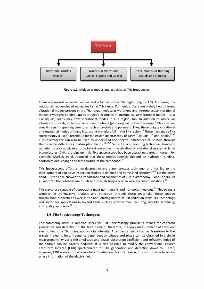
Figure 1.2 Molecular modes and activities at THz frequencies. ..................................................... 3

Figure 2.1 Picture of the Ti:Sapphire Laser and Verdi V5 in the THz Research Laboratory, in

Physics Department, at METU. ...................................................................................... 8

Figure 2.2 Schematic diagram of the THz-TDS system. .................................................................. 9

Figure 2.3 (a) Front view on mounted PCA (laser side). (b) Back view on mounted PCA (THz

side). ............................................................................................................................ 10

Figure 2.4 Dimensions of the PC antenna. ................................................................................... 10

Figure 2.5 Transient electric field of THz pulse in time domain. .................................................. 11

Figure 2.6 A screen-shot of Labview software. ............................................................................ 12

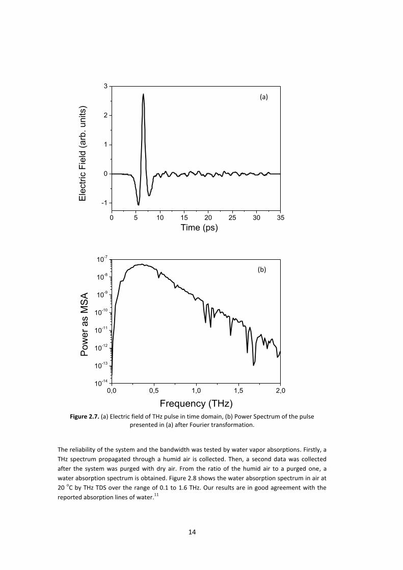
Figure 2.7 (a) Electric field of THz pulse in time domain, (b) Power Spectrum of the pulse

presented in (a) after Fourier Transformation. ........................................................... 14

Figure 2.8 Absorption spectrum of water at 20 o

C (solid line). Dashed lines are from

reference 11. ............................................................................................................... 15

Figure 3.1 THz E-field spectra of fuel oils in time domain. ........................................................... 19

Figure 3.2 (a) Index of refraction, (b) absorption coefficient and, (c) real part of permittivity (ε')

of fuel oils as functions of frequency. ......................................................................... 20

Figure 3.3 THz pulse profiles of gasoline, ethanol and their mixtures at varying mix ratios. ....... 21

Figure 3.4 Power transmission spectra derived from Fast Fourier Transform of the data in ...... 22

Figure 3.5 (a) Graph of THz peak amplitude vs. ethanol concentration. Cross symbols are

experimental values, solid line is an exponential fitting. (b) Graph of delay time

relative to gasoline vs. percent ethanol. Star symbols are experimental data and solid

line is a linear fitting. ................................................................................................... 23

Figure 3.6 Comparison of frequency dependent refractive index (a) and absorption coefficient

(b) of gasoline-ethanol mixtures. ................................................................................ 25

Figure 3.7 Real part of permittivity data of pure ethanol, gasoline and their mixtures. ............. 26

Figure 3.8 Experimental real (a) and imaginary (b) part of permittivity data (circles) for ethanol

together with the fit of triple Debye relaxation model (solid line). ............................ 27

Figure 3.9 Experimental real (a) and imaginary (b) part of permittivity data (circles) for gasoline

together with the fit of double Debye relaxation model (solid line). .......................... 28

Figure 3.10 Experimental real (a) and imaginary (b) part of permittivity data (circles) for mixtures

of gasoline-ethanol together with the double-Debye relaxation model (solid line). .. 30

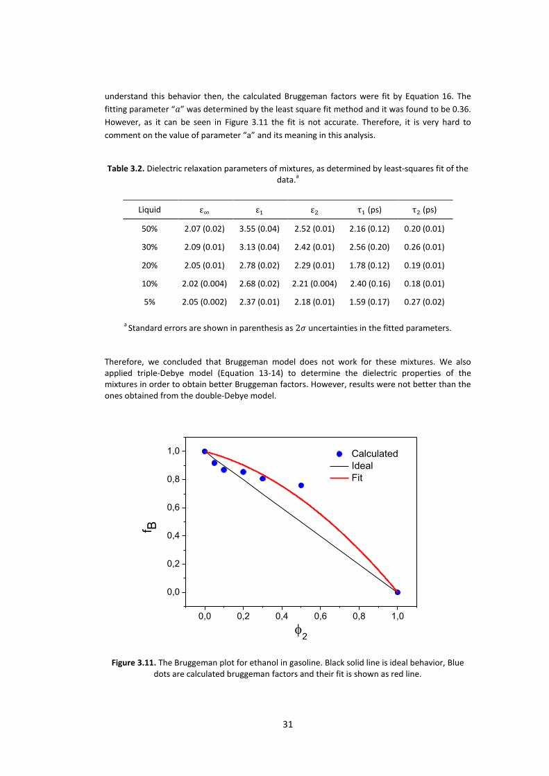
Figure 3.11 The Bruggeman plot for ethanol in gasoline. Black solid line is ideal behavior, Blue

dots are calculated bruggeman factors and their fit is shown as red line. .................. 31

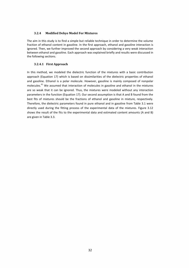
Figure 3.12 Experimental real (a) and imaginary (b) part of permittivity data (circles) for mixtures

of gasoline-ethanol together with the improved Debye relaxation model (solid

line)…… ........................................................................................................................ 33

Figure 3.13 Values of A (red circles) found from the best fits of the mixtures’ data. Black line is

experimental values of A. ............................................................................................ 34

Figure 3.14 The improved Debye relaxation model (solid line) along with the real (a) and

imaginary (b) part of permittivity data (circles) derived from the experimental

measurements for the mixtures of ethanol and gasoline. .......................................... 36

Figure 3.15 Values of A (red circles) found from the best fits of the mixtures’ data. Black line is

experimental values of A. ............................................................................................ 38

xii

1

CHAPTER 1

INTRODUCTION It is possible to analyze materials in the electromagnetic region ranging from radiowaves to gamma-rays. In each region of electromagnetic spectrum, different properties of a material can be studied. Terahertz rays (T-rays) are low energetic waves which can penetrate through a wide variety of materials and provide unique optical properties of the material probed. In recent years, the Terahertz (THz) spectral region has seen a flurry of research activities in many different areas. In this thesis, the highlights of THz research and spectroscopy will be mentioned briefly, and its feasibility towards the investigation of dielectric properties of fuel oils and their mixtures will be discussed in detail.

1.1 Terahertz Radiation Tera is a prefix, denoting

10

12 and Hertz is the SI unit of the frequency (s

-1). Thus, 1 Terahertz

(THz) corresponds to 1012

Hertz in frequency. In other units, 1 THz is equivalent to ~300μm wavelength, ~33.33cm

–1 wavenumbers, ~4.1meV energy, and ~48K temperature. In

electromagnetic spectrum, THz region lies between microwave and infrared regions with overlaps in both (Figure 1.1). This region is generally considered to be from 0.1 THz to 10 THz.

1

Figure 1.1. Electromagnetic spectrum.

1.2 A Brief History Although the usage of THz waves in various areas has been a hot topic in the past two decades, its origin is based on the studies performed in the last century.

2 In between 1890-1924, scientists

carried out studies on generation and detection of millimeter waves.2 Fortunately, Nichols and

Tear were able to produce and detect waves with in the range of 7mm-0.22 mm (0.04-1.36 THz) in the 1920’s.

3 Then, Glagolewa-Arkadiewa created waves from 50 mm to 0.082 mm (0.006-3.7

THz) in 1924.3 It was after 1965 that the evolutionary developments in laser systems made the

lasers suitable to be used as sources for THz studies.4 Pulsed lasers has enabled the development

of time dependent methods to record the THz signal. It was in 1984, when Austin, Cheung and Smith succeeded to produce and detect 1.6 ps (0.625 THz) broadband THz electromagnetic pulses by using photoconductive (PC) switch method driven by a pulsed laser.

5 In the following

year, the first article that reported THz wave generation and detection via PC antenna was

2

published by Smith, Auston and Nuss.6 They designed a PC antenna based on radiation-damaged

silicon-on-sapphire semiconductor and used it for both as an emitter and a detector. In their study, they obtained 0.1-2.0 THz bandwidth. Nonlinear optical process is another efficient technique for THz generation. The process behind this technique is directly related to second order nonlinear optical property of the crystals (ZnTe, GaP etc.). In the beginning of 1970’s, Yajima et al.

7 and Yang et al.

8 were the frontiers who used nonlinear crystals for THz generation.

The strength of this technique is that it can give a much broader spectral bandwidth compared to PC antennas. In addition similar nonlinear crystals can also be used as a THz detector. In the following sections, THz generation and THz detection methods will be explained in detail.

1.3 THz Generation Methods There are two common ways to produce THz radiation; nonlinear optical process and PC antenna (PCA). PCA is the oldest method for the THz generation.

9 It is based on the process of using a

femtosecond laser pulse to generate charge carriers in the conduction band of a semiconductor under an applied bias voltage.

9 Generally, a few nanojoule per pulse femtosecond optical beam is

focused on the antenna to generate and accelerate charge carriers. Bias provides that all the carriers move in the same direction. The acceleration of the carriers results in emission of an electromagnetic radiation in the THz region. Although the conversion efficiency obtained using a nonlinear crystal is not as high as that obtained with PCA method, nonlinear optical process is still a powerful method for many applications such as time-domain spectroscopy or imaging with its broader bandwidth. In this method, the optical pulse with a certain range of frequencies (usually between visible and near-infrared) propagating in a nonlinear medium result in wave mixing process such as difference frequency generation. The generated difference frequencies fall in THz range and form THz transient.

9 ZnTe, GaAs, and GaP are the most commonly used nonlinear crystals for THz

generation.

1.4 THz Detections Methods THz detection can be done either by PCA or free space Electro-Optic (EO) sampling. The process of detection with PCA is very similar to the generation process. Without an applied bias voltage, electron hole pair on the substrate is formed by an optical pulse and free carriers are driven by the electric field of the incoming THz pulse. Current formed by the movement of the charge carriers is detected and recorded as a voltage. The time dependent voltage characteristics of the process gives THz pulse.

9 On the other hand, EO crystals are commonly used materials for the

free space electro-optic sampling method. Basically, both THz and optical pulse propagate through a nonlinear crystal. The THz beam modifies the index of the EO crystal transiently, via the Pockel’s effect.

10 This changes the polarization of optical pulse that is passing through the crystal.

Then, the change in the polarization is probed by a balanced photodetector. The data directly correlates with the THz electric field.

11

1.5 Applications of THz Waves

In electromagnetic spectrum, materials show difference due to their spectral fingerprints depending on the working frequency range. Thus, scientists have been developing instruments covering as much of the electromagnetic range as possible. The THz region was considered a gap previously due to the unavailability of powerful sources and sensitive detectors. However, it has been a popular one that have attracted scientists, recently.

9

3

Figure 1.2. Molecular modes and activities at THz frequencies. There are several molecular modes and activities in the THz region (Figure 1.2). For gases, the rotational frequencies of molecules fall in THz range. For liquids, there are mainly two different vibrational modes present in the THz range; molecular vibrations and intermolecular vibrational modes. Hydrogen bonded liquids are good examples of intermolecular vibrational modes.

12 Just

like liquids, solids may have vibrational modes in THz region, too. In addition to molecular vibrations in solids, collective vibrational motions (phonons) fall in the THz range.

1 Phonons are

usually seen in repeating structures such as crystals and polymers. Thus, these unique vibrational and rotational modes of many interesting materials fall in the THz region.

13 These have made THz

spectroscopy a useful technique for molecular spectroscopy of gases14

, liquids

15,16 and, solids.

17,18

THz spectroscopy can also be used to understand the spectral differences of isomers through their spectral differences in absorption bands.

12,19,20 Since it is a nonionizing technique, Terahertz

radiation is also applicable to biological molecules. Investigation of vibrational modes of large biomolecules (DNA, proteins etc.) via THz spectroscopy has been attracting a great interest. For example, Markelz et al. reported that these modes strongly depend on hydration, binding, conformational change and temperature of the compound.

21

THz Spectroscopy offers a non-destructive and a non-contact technique, and has led to the development of explosive inspection studies in defense and home-land security.

22–24 On the other

hand, Burton et al. showed the importance and capabilities of THz in astronomy25

, and Federici et al. reported the potential use of THz and sub-THz frequencies in wireless communications.

26

THz waves are capable of penetrating most non-metallic and non-polar mediums.

27 This opens a

window for noninvasive analysis and detection through these materials. These unique transmission properties as well as the non-ionizing nature of THz radiation make THz technology well-suited for applications in several fields such as polymer manufacturing, security, screening, and quality assurance.

28

1.6 THz Spectroscopy Techniques

The commonly used Ti:Sapphire lasers for THz Spectroscopy provide a means for coherent generation and detection in the time domain. Therefore, it allows measurement of transient electric field of a THz pulse, not only its intensity. After performing a Fourier Transform to the transient electric field, frequency dependent amplitude and phase can be obtained in a single measurement. By using the amplitude and phase, absorption coefficient and refractive index of the sample can be directly deduced. It is also possible to modify the conventional Fourier Transform Infrared (FTIR) spectrometer for THz generation and detection down to 5 cm

-1;

however, FTIR sources provide incoherent detection. For this reason, it is not possible to obtain phase information of the electric field.

Inter-molecular Bonding

(Solids and Liquids)

Rotational Modes

(Gases)

Molecular Vibrations

(Solids, Liquids and Gases)

THz Waves

4

THz Time-Domain Spectroscopy (THz-TDS) is probably the most commonly used and accessible technique for chemists and chemistry applications. In THz-TDS, there are two arms making up the spectrometer; generation arm and detection arm. THz wave is produced in generation arm and it is probed by the optical beam through the detection arm. The static properties of samples which are absorption coefficient and refractive index can be obtained by this technique. Another advantage of THz spectrometers based on pulsed femtosecond Ti:Sapphire lasers is its sub-picosecond time resolution. Thus, photoexcited samples can be probed and dynamics of these processes can be investigated with picosecond resolution via Time-Resolved THz spectroscopy (TRTS). Basically, the sample is photoexcited with an ultrafast pulse laser (with energy ranging from UV to mid-IR). After a while (delay time may be tuned from 100 fs to several ns), the THz beam propagates through the sample and the change of THz transient in time is probed. A significant application of TRTS is the investigation of semiconductor photophysics.

29

Conductivity and carriers dynamics of the sample can also be obtained by TRTS technique.30

1.7 The Aim of This Study Although many alternative energy sources are available today, petroleum based fuels are still the major energy source of the world.

31 Commercially available petroleum based fuels, which are

used in combustion engines, are mixtures that include a large number of variety of molecules such as paraffin, aromatic compounds, cycloalkanes and asphaltene.

32 In addition to these

compounds, fuel additives can also be used for enhancing fuel performance and also for lowering exhaust emissions.

33,34 Methanol, ethanol, tertiary butyl alcohol, and methyl tertiary butyl ether

are just a few examples of oxygenated compounds used as fuel additives.33

Among those compounds ethanol, an environmentally friendly additive, is the commonly used one.

33 The

allowed usage amount of ethanol in gasoline depends on the country regulations. USA Environmental Protection Agency allows up to %15 ethanol to be blended with gasoline.

35

Whereas, regulations in Europe allows the ethanol percent in petroleum products to be 10%.36

In Turkey, Energy Community Regulatory Board decided that in 2013 minimum ethanol percent in fuel oil will be 2% (v/v), and in 2014 this value will increase to 3% (v/v).

37 Therefore, it is deeply

crucial to control the amount of ethanol in fuel oil. To make sure that an excess amount of ethanol is not added to the gasoline, a simple and reliable technique is needed. In this study, we present a new and a simple technique for the detection of amount of ethanol in fuel oil. Near-IR and Mid-IR analysis of petroleum products have been widely studied and published.

38–40

In 2006, Al-Douseri et al.

showed the potential use of far-IR and THz spectroscopy on investigation of petroleum products.

41 In 2008, optical properties of petroleum products and

their mixtures with organic solvents (xylene, toluene and benzene) in THz range were investigated and reported by Jin et al.

42 and Kim et al.

43 The analysis of gasoline-ethanol mixtures

was conducted in near-IR range44

; however, there is no study in the literature that discuss the effects of ethanol on the optical properties of gasoline in the THz range. Here, we report the terahertz optical properties of gasoline, diesel and 5, 10, 20, 30, 50 % mixtures of ethanol and gasoline. THz-TDS is a suitable technique for the analysis of a wide variety of liquids, especially the ones containing OH groups. It is a powerful technique that enables the study of inter- and intra-molecular modes of molecules. For example, Yomogida et al. investigated the complex permittivity of various alcohols using THz-TDS, and concluded that THz waves are capable of analyzing the molecular dynamics of both dielectric and vibrational relaxation of hydrogen bonded liquids.

12 On the other hand dielectric response of pure solvents and their mixtures to

THz radiation has gained a significant attention over the past two decades, due to the need to understand how solvation dynamics occur on time scales of a few picoseconds. Up to now, using

5

this technique dynamical response of pure liquids including water, alcohols, benzenes has been widely studied.

45–47 It was shown that Debye-based dielectric relaxation model provides a good

estimation to the relaxation steps of pure liquids and their mixtures. The interaction between liquids in binary mixtures can be modeled well by Bruggeman Model.

48,49 The applicability of this

model to ethanol mixtures of gasoline is also discussed and compared with our modified Debye Model. In this thesis, using the modified Debye-Model and THz-TDS, we were able to develop a new method for the detection of ethanol in gasoline. The outline of this thesis as follows: In Chapter 2, the instrumental set-up is explained in detail and also theory and calculations are given. In Chapter 3, the experimental results are given and different modeling techniques are discussed in detail. Finally, the study is concluded in the last chapter.

6

7

CHAPTER 2

EXPERIMENTAL In this study, we constructed a THz Time-Domain Spectrometer in the THz Research Laboratory, in Physics Department at Middle East Technical University (METU). The THz-TDS set-up includes the following components;

Ti: Sapphire Mode-Lock Laser (Coherent Verdi-V5 pumped Femtolaser Gmbh)

Beam splitter (85% Transmission-15% Reflection)

Mirrors

Attenuation filters

Objective

Batop Photoconductive Antenna (PCA-40-05-10-800-h)

Off axis parabolic mirrors (OAPM)

Polymethylpentene (TPX) lenses (focal length = 10 cm)

Lens (focal length = 20 cm)

<110> ZnTe crystal, 2mm thickness

Quarter (λ/4) wave plate

Wollaston prism

Large-area balanced photodetector

Motorized translation stage

Function generator

Stanford Research System SR830 Lock-in Amplifier

Computer with National Instruments Labview software Each component of the set-up will be briefly mentioned in the following sections.

2.1 Laser Source Mode-locked Ti:Sapphire lasers are commonly used for ultrafast studies due to their tunability and ability to generate ultra-short pulses. In this thesis, mode-locked Ti:Sapphire laser was used as an optical source for the spectrometer. Briefly, Ti:Sapphire laser refers to the lasing medium of sapphire crystal (Al2O3) which is doped with Ti

3+ ions. Mode-locked Ti:Sapphire laser is pumped

by Verdi V5, which is a source of green laser light. Ti:Sapphire crystal absorbs the green light and produces red light with a center-wavelength near 800 nm. When the beam is mode-locked, 20 fs pulses with the 350 mW average power at 75 MHz repetition rate are ready to be used for scientific studies. Mode-locked Ti:Sapphire laser and Verdi V5 used in this thesis are shown in Figure 2.1.

8

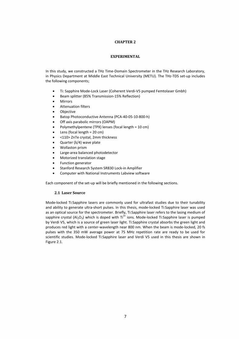
These systems are very sensitive to the changes in ambient temperature and humidity. For this reason, a central air conditioning unit is used. Temperature and humidity are systematically followed up and recorded. A secondary air conditioner is always ready to use in extremely cold or hot days of the year.

2.2 THz Time Domain Spectrometer Figure 2.2 demonstrates the schematic diagram of the THz Time Domain Spectrometer which was constructed for THz transmission studies of samples. Light at 800 nm wavelength used in the set-up is provided by the previously described Ti:Sapphire laser. Briefly, a beam splitter divides the beam into two arms; the transmitted one is used for generating THz waves via PCA method and the reflected one (optic sampling beam) is used for EO detection via ZnTe crystal. The purpose of attenuator filters in each arm is to lower the energy of the beam to optimize values. The generation and detection processes are explained in detail in the following sections. The generated THz beam were collimated with and focused onto the crystal by a pair of off-axis parabolic mirrors (OAPM), and a polymethylpentene (TPX) lens with 100 mm focal length, which focused the THz beam to a maximum spot diameter of 8 mm. Both THz beam and optic sampling beam propagate through a 2 mm thick ZnTe crystal at the same time. Given that the both pulses are very short in time (< ps) it is very difficult to have them overlap on the crystal at the same time. To do this, the distances in both two arms should be measured and equalized very carefully. The errors in distances are corrected by a motorized delay stage. The optic beam passing through the crystal is detected thorugh a balanced photodetector after passing through a λ/4 wave-plate and a wollaston prism.

Verdi V5

Ti:Sapphire

Figure 2.1. Picture of the Ti:Sapphire Laser and Verdi V5 in the THz Research Laboratory, in Physics Department, at METU.

9

Figure 2.2. Schematic diagram of the THz-TDS system.

The signal received from the balanced photodetector is amplified by a Lock-in Amplifier. Then, it is transferred to the digital medium by a computer. We used Labview software in order to control motorized delay stage and to encode the signal from Lock-in. In the following sections, the system is explained in detail.

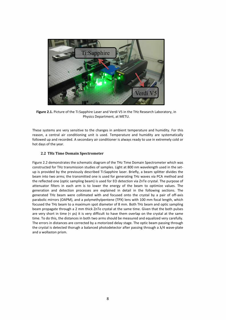
2.2.1 Terahertz Generation via PCA Method In our set-up, we used PCA-40-05-10-800-h manufactured by BATOP. The close up pictures of the antenna taken from BATOP website is given in Figure 2.3.

50 Semi-insulating GaAs forms the

substrate with 6mmx6mm chip area. The PCA is mounted on hyperhemispherical silicon substrate lens.

Sample

Attenuator Filter

Beam Splitter

Motorized Delay Stage

Ti:Sapphire Laser

Balanced Photodetector

PCA

ZnTe Crystal

Attenuator Filter

Objective

OAPM OAPM

Lens

λ/4 Plate

Wollaston

Lockin Amplifier

Voltage Generator

10

Figure 2.3. (a) Front view on mounted PCA (laser side), (b) Back view on mounted PCA (THz side). Pictures were taken from BATOP website.

50

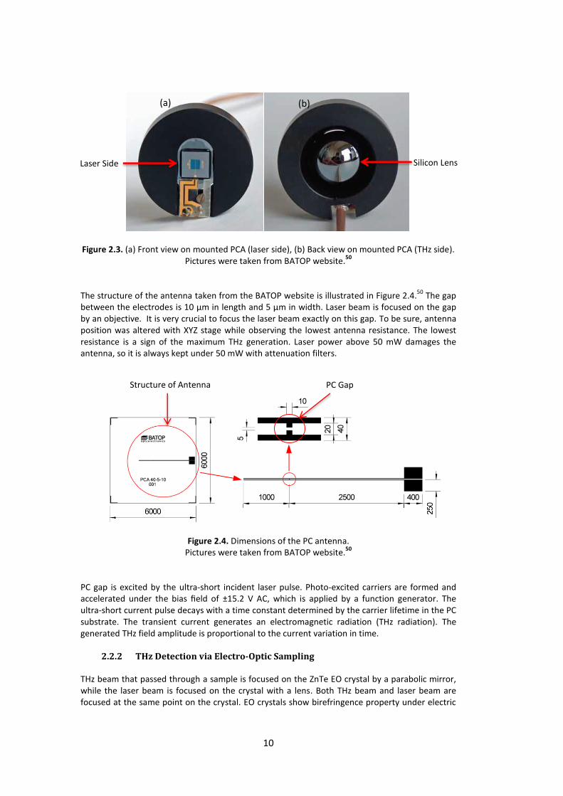
The structure of the antenna taken from the BATOP website is illustrated in Figure 2.4.

50 The gap

between the electrodes is 10 µm in length and 5 µm in width. Laser beam is focused on the gap by an objective. It is very crucial to focus the laser beam exactly on this gap. To be sure, antenna position was altered with XYZ stage while observing the lowest antenna resistance. The lowest resistance is a sign of the maximum THz generation. Laser power above 50 mW damages the antenna, so it is always kept under 50 mW with attenuation filters.

Figure 2.4. Dimensions of the PC antenna. Pictures were taken from BATOP website.

50

PC gap is excited by the ultra-short incident laser pulse. Photo-excited carriers are formed and accelerated under the bias field of ±15.2 V AC, which is applied by a function generator. The ultra-short current pulse decays with a time constant determined by the carrier lifetime in the PC substrate. The transient current generates an electromagnetic radiation (THz radiation). The generated THz field amplitude is proportional to the current variation in time.

2.2.2 THz Detection via Electro-Optic Sampling THz beam that passed through a sample is focused on the ZnTe EO crystal by a parabolic mirror, while the laser beam is focused on the crystal with a lens. Both THz beam and laser beam are focused at the same point on the crystal. EO crystals show birefringence property under electric

(a) (b)

Laser Side Silicon Lens

Structure of Antenna PC Gap

11

field such as THz field. When it happens, EO crystal has different refractive indices along two of its axes. This results in a change in the polarization of laser beam. Magnitude of the polarization change in the laser beam is directly proportional to the magnitude of the THz field. With the use of a quarter-wave plate and a Wollaston prism to separate the polarizations, the intensities of each polarization is recorded by a detector as a function of time as laser pulse is delayed with respect to the THz pulse. Thus, the recorded intensity versus time spectrum is directly proportional to the THz electric field.

9 The aim of the usage of λ/4 wave plate is to balance the

intensities and ensure zero the signal when there is no THz radiation. On the other hand, the Wollaston prism separates the components of the light beam which are perpendicular to the table surface and parallel to the table surface. The balanced photodetector response is amplified by the use of the Lock-in Amplifier, which is synchronized to the modulation on the PCA. Thus, Lock-in not only amplifies the signal but also lowers the noise and enhances Signal to Noise (S/N) ratio. A typical time dependent THz pulse profile collected in our system is shown in Figure 2.5.

0 15 30 45 60-1

0

1

2

Ele

ctr

ic F

ield

(a

rb.

un

its)

Time (ps)

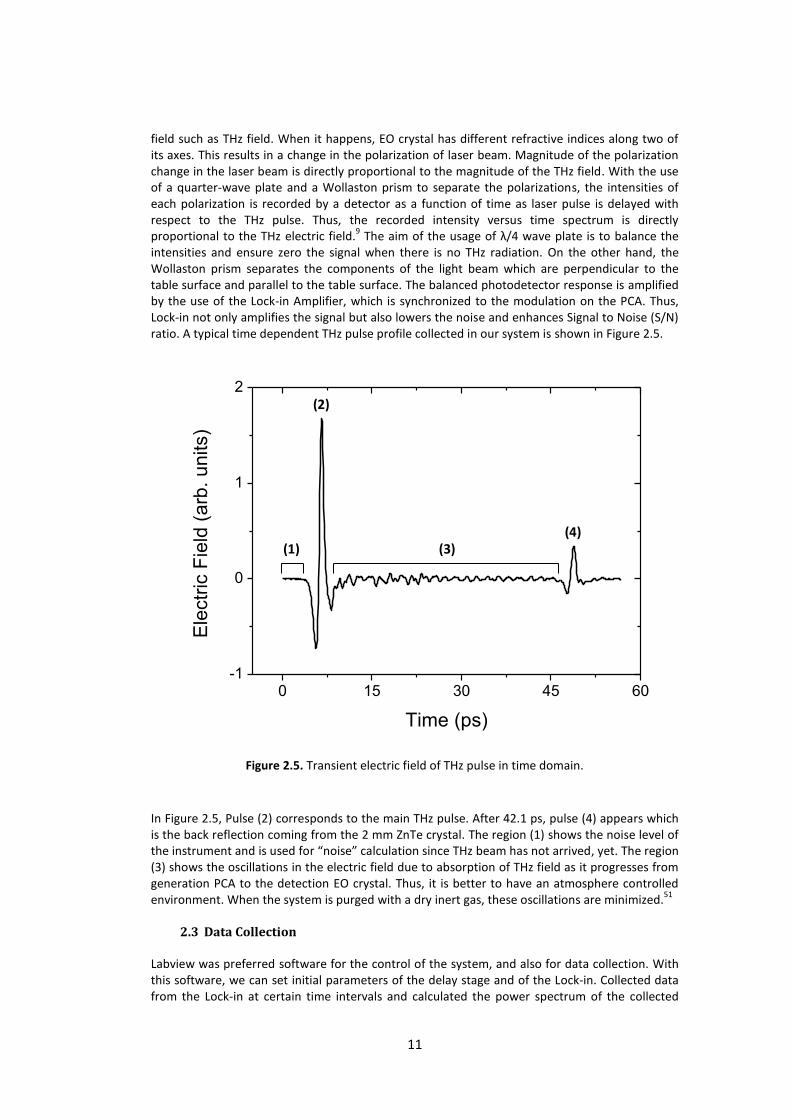
Figure 2.5. Transient electric field of THz pulse in time domain.

In Figure 2.5, Pulse (2) corresponds to the main THz pulse. After 42.1 ps, pulse (4) appears which is the back reflection coming from the 2 mm ZnTe crystal. The region (1) shows the noise level of the instrument and is used for “noise” calculation since THz beam has not arrived, yet. The region (3) shows the oscillations in the electric field due to absorption of THz field as it progresses from generation PCA to the detection EO crystal. Thus, it is better to have an atmosphere controlled environment. When the system is purged with a dry inert gas, these oscillations are minimized.

51

2.3 Data Collection

Labview was preferred software for the control of the system, and also for data collection. With this software, we can set initial parameters of the delay stage and of the Lock-in. Collected data from the Lock-in at certain time intervals and calculated the power spectrum of the collected

(2)

(4) (3) (1)

12

data are shown in Figure 2.6. All is done by the written codes in the Labview environment specific to our electronic components in the system. During the data collection, we progressively (at certain time intervals) change the position of the optical pulse by the motorized delay stage in time domain with the help of the software code. By doing so, the profile of THz pulse in time is scanned by the ultra-short laser pulse and the electric field of THz pulse is obtained in time with a resolution determined by the step size of the delay stage movement. The scan step, thus the time step, of the motorized delay stage is very important for collecting a true profile of the THz pulse in time. Before collecting data, the position of the pulse is recorded and the step size and scan length (starting position and final position) are decided. During a scan, a typical step consists of three main steps; movement of the stage by 10 micron (the step size), stop and wait for 600 millisecond, and read the value of signal in voltage from the Lock-in. This step is repeated until the stage reaches its final position. After the scan is completed, the data is saved as voltage vs. time where the time is the relative time of the optical arm (detection light) with respect to the THz arm and determined from the stage micrometer positions. Once the system is optimized for the best THz profile the scanning parameters are kept same for all the experimental measurements. For the current set-up, the optimum parameters are; 10 µm step and 600 ms wait time. Since the light travels twice the distance relative to the delay stage, each 10 µm step in fact corresponds to 20 µm change in position of the optic pulse. This corresponds to a 0.067 ps time interval between each data point.

Figure 2.6. A screen-shot of Labview software.

Power Spectrum

Stage Position

Electric Field

vs. Time

13

To conduct reliable measurements, we test the system by comparing data collected before and after measurement of samples, which is going to be referred as air spectrum from now on. If these two air spectra are similar within the reasonable system noise, then collected data is reliable. Otherwise it is not reliable and system should be checked for any changes. By doing so, we have a chance to see the possible changes in the spectrometer, and also in the laser source. The terahertz spectroscopic measurements are similar to the FTIR or UV spectroscopic measurements and it always requires a reference measurement. One important point for correct measurement of the sample is that the scan length of the reference and sample measurements must be the same.

2.4 Data Processing After the collection of the data, they are saved to a file and processed by one of commercially available data processing softwares such as Mathematica, Origin or Igor. Data processing may require editing the available data for removing reflections, padding for Fast Fourier Transform (FFT), etc. One must be very careful during the editing process and should pay extra attention on not to manipulate the original data itself when deleting, adding or padding. FFT of the time domain data results in both amplitude and phase values of the terahertz electric field at discrete frequencies. The calculations of the optical parameters of samples are mentioned in detail in the following section.

2.5 Theory and Calculations In order to convert the time domain spectrum into a frequency domain, along the THz system optical axis, , a Fourier transform is applied. The Fourier transform of the time-resolved electric field gives the relative amplitude and phase of each frequency component of the THz pulse.

51

∫

(1)

is the complex electric field and is the experimentally measured THz electric field as a function of time. Figure 2.7a displays a THz pulse generated by PCA method and detected by ZnTe crystal. Figure 2.7b shows the power spectrum after the Fourier transform. Well resolved-absorption lines in the power spectrum are due to water vapor in air. The spectrometer has a bandwidth of 1.6 THz with a S/N ratio 10

5/1.

14

0 5 10 15 20 25 30 35

-1

0

1

2

3

Time (ps)

Ele

ctr

ic F

ield

(arb

. u

nits)

0,0 0,5 1,0 1,5 2,010

-14

10-13

10-12

10-11

10-10

10-9

10-8

10-7

Pow

er

as M

SA

Frequency (THz)

Figure 2.7. (a) Electric field of THz pulse in time domain, (b) Power Spectrum of the pulse presented in (a) after Fourier transformation.

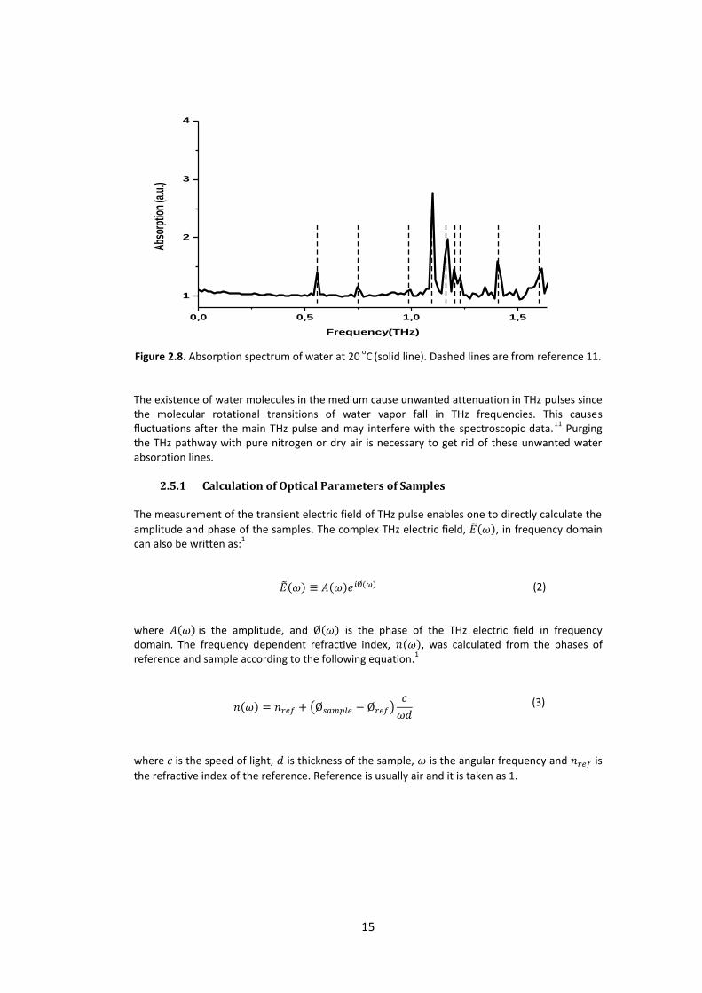
The reliability of the system and the bandwidth was tested by water vapor absorptions. Firstly, a

THz spectrum propagated through a humid air is collected. Then, a second data was collected

after the system was purged with dry air. From the ratio of the humid air to a purged one, a

water absorption spectrum is obtained. Figure 2.8 shows the water absorption spectrum in air at

20 oC by THz TDS over the range of 0.1 to 1.6 THz. Our results are in good agreement with the

reported absorption lines of water.11

(a)

(b)

15

Figure 2.8. Absorption spectrum of water at 20

oC

(solid line). Dashed lines are from reference 11.

The existence of water molecules in the medium cause unwanted attenuation in THz pulses since the molecular rotational transitions of water vapor fall in THz frequencies. This causes fluctuations after the main THz pulse and may interfere with the spectroscopic data.

11 Purging

the THz pathway with pure nitrogen or dry air is necessary to get rid of these unwanted water absorption lines.

2.5.1 Calculation of Optical Parameters of Samples The measurement of the transient electric field of THz pulse enables one to directly calculate the

amplitude and phase of the samples. The complex THz electric field, , in frequency domain can also be written as:

1

(2)

where is the amplitude, and is the phase of the THz electric field in frequency domain. The frequency dependent refractive index, , was calculated from the phases of reference and sample according to the following equation.

1

( )

(3)

where is the speed of light, is thickness of the sample, is the angular frequency and is

the refractive index of the reference. Reference is usually air and it is taken as 1.

0,0 0,5 1,0 1,5

1

2

3

4

Abs

orpt

ion

(a.u

.)

Frequency(THz)

16

Similarly, the absorption coefficient was determined from the amplitude of the sample and the reference data

1:

(

) (4)

Complex dielectric function is composed of real and imaginary components;

(5)

The complex dielectric function, , is calculated through where

and

.Thus, frequency dependent real and imaginary part of dielectric function are

obtained from and ;

(6)

and

(7)

2.5.2 Debye Model Dielectric function is a measure of the polarizability of a sample. For liquids, dielectric function can be modeled through the use of Debye model. When an external field is applied to a liquid, the molecules polarize. After a while, this polarization disappears and molecules relax back to its initial state. The time elapsed during this relaxation is called relaxation time, τ. Barthel et al. used Debye relaxation process for a variety of solvents in GHz range.

52 Kindt et. al. extended this range

up to 1 THz for polar liquids.45

A general expression for describing complex dielectric function, , according to the Debye model is;

52

∑

(8)

where is dielectric constant at high frequency limit, is the dielectric constant at zero frequency, are intermediate values of the real part of the dielectric constant, and is the

Debye relaxation time that corresponds to the jth relaxation process. Parameters and are

used for modification of the Debye model toward Cole-Cole or Cole-Davidson, in order to depict a continuous distribution of relaxation times in the medium.

53–56 A Cole-Cole treatment (

, ) describes a symmetric distribution about , while a Cole-Davidson treatment

( , ) describes a assymetric distribution.52

Both treatments can be applied to

17

single or multiple Debye processes. Ethanol was successfully modeled without Cole-Cole or Cole-Davidson treatments by the previous workers.

52,57 For this reason, Cole-Cole or Cole-Davidson

treatments were not considered for the pure ethanol, gasoline and their mixtures in this study. Thus, and were held fixed at 0 and 1, respectively. Modeling the liquids is discussed in a

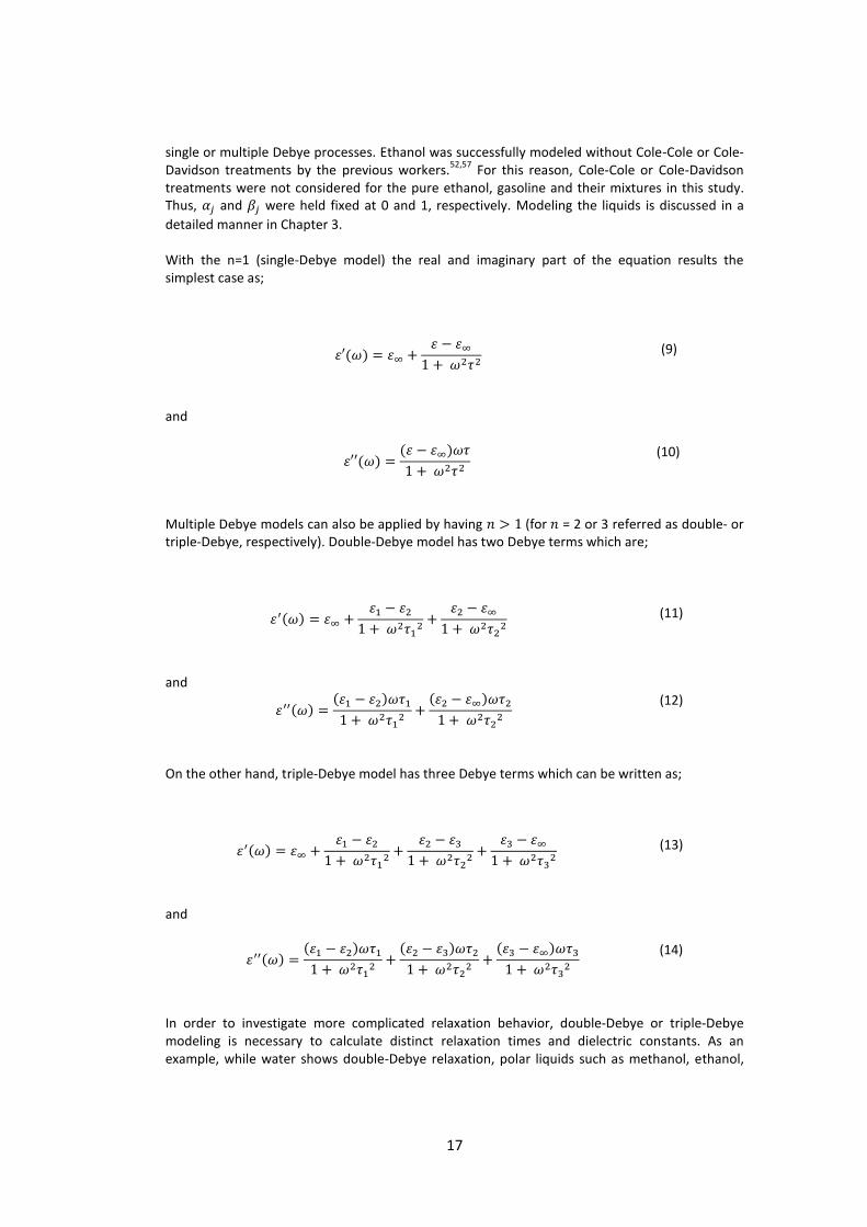
detailed manner in Chapter 3. With the n=1 (single-Debye model) the real and imaginary part of the equation results the simplest case as;

(9)

and

(10)

Multiple Debye models can also be applied by having (for = 2 or 3 referred as double- or triple-Debye, respectively). Double-Debye model has two Debye terms which are;

(11)

and

(12)

On the other hand, triple-Debye model has three Debye terms which can be written as;

(13)

and

(14)

In order to investigate more complicated relaxation behavior, double-Debye or triple-Debye modeling is necessary to calculate distinct relaxation times and dielectric constants. As an example, while water shows double-Debye relaxation, polar liquids such as methanol, ethanol,

18

propanol exhibit triple-Debye relaxation process.58

In this study, we have applied triple-Debye model for pure ethanol, and a double-Debye model for gasoline.

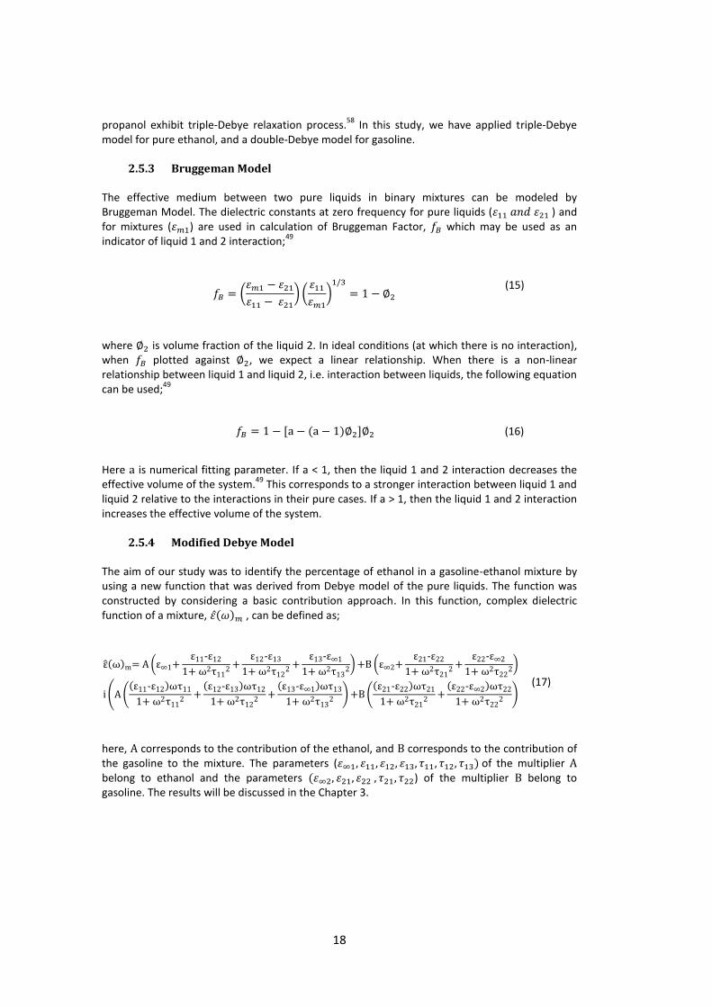
2.5.3 Bruggeman Model The effective medium between two pure liquids in binary mixtures can be modeled by Bruggeman Model. The dielectric constants at zero frequency for pure liquids ( ) and for mixtures ( ) are used in calculation of Bruggeman Factor, which may be used as an indicator of liquid 1 and 2 interaction;

49

(

) (

)

(15)

where is volume fraction of the liquid 2. In ideal conditions (at which there is no interaction), when plotted against , we expect a linear relationship. When there is a non-linear relationship between liquid 1 and liquid 2, i.e. interaction between liquids, the following equation can be used;

49

(16)

Here is numerical fitting parameter. If a < 1, then the liquid 1 and 2 interaction decreases the effective volume of the system.

49 This corresponds to a stronger interaction between liquid 1 and

liquid 2 relative to the interactions in their pure cases. If a > 1, then the liquid 1 and 2 interaction increases the effective volume of the system.

2.5.4 Modified Debye Model The aim of our study was to identify the percentage of ethanol in a gasoline-ethanol mixture by using a new function that was derived from Debye model of the pure liquids. The function was constructed by considering a basic contribution approach. In this function, complex dielectric function of a mixture, , can be defined as;

(

) (

)

( (

) (

))

(1 (17)

here, corresponds to the contribution of the ethanol, and corresponds to the contribution of the gasoline to the mixture. The parameters ( of the multiplier belong to ethanol and the parameters ) of the multiplier belong to gasoline. The results will be discussed in the Chapter 3.

19

CHAPTER 3

RESULTS AND DISCUSSION Liquid fuel oil samples (diesel and gasoline) were obtained from Petrol Ofisi. All the measurements were conducted just after they were received from the station. Pure ethanol was used to prepare 5, 10, 20, 30, 50% (percent ethanol) mixtures of ethanol and gasoline. The liquid samples were introduced at the focal point of the THz light in a 2mm thick quartz cuvette holder. All calculations were done according to the equations given in section 2.5. This chapter is divided into two sections; measurement of pure fuel oils and measurement of gasoline-ethanol mixtures.

3.1 Measurement of Pure Fuel Oils Pulse profiles of the transmitted THz field through reference (empty cell), diesel, and gasoline are shown in Figure 3.1. Reference is an empty (air filled) quartz sample holder. FFT of time domain data results in amplitude and phase of each sample liquid and the reference. Then we calculated refractive index, absorption coefficient and dielectric constant of fuel oils in frequency domain (Figure 3.2).

9 12 15 18 21 24 27

-2

-1

0

1

2

3

4

5

Reference

Gasoline

Diesel

TH

z E

-Fie

ld (

arb

. u

nits)

Time (ps)

Figure 3.1. THz E-field spectra of fuel oils in time domain. Refractive index of diesel was found to be higher than that of gasoline. Gasoline has higher absorption coefficient than that of the diesel at all frequencies. For both fuel oils, absorption coefficient shows a growth as the frequency increases. This growth could be a sign of an absorption feature at higher frequencies since it was shown that the absorption fingerprints of gasoline in far-infrared starts at 4.5 THz

41 or it could be due to dipole-dipole interactions in the

liquid. Calculated dielectric constants are shown in Figure 3.2c. The differences in optical parameters are most likely due to the diversity in concentrations of the main ingredients of two fuel oils. The most significant difference between diesel and gasoline is their carbon chain lengths. The average values of hydrocarbon formula for diesel and gasoline are C14H30 and C9H20,

20

respectively.59

These clear differences in optical parameters shown in this study emphasize that THz-TDS is capable of easily identifying different type of fuel oils.

0,2 0,3 0,4 0,5 0,6 0,7 0,8 0,9 1,0 1,11,41

1,42

1,43

1,44

1,45

1,46

1,47

1,48

1,49

Gasoline

DieselR

efr

active Index

Frequency (THz)

0,2 0,3 0,4 0,5 0,6 0,7 0,8 0,9 1,0 1,1

0

2

4

6

8

10

Gasoline

Diesel

Absorp

tion C

oeffic

ient(

cm

-1)

Frequency(THz)

0,2 0,3 0,4 0,5 0,6 0,7 0,8 0,9 1,0 1,1

2,01

2,04

2,07

2,10

2,13

2,16

2,19

2,22

Diesel

Gasoline

Frequency(THz)

'

Figure 3.2. (a) Index of refraction, (b) absorption coefficient and, (c) real part of permittivity (ε')

of fuel oils as functions of frequency.

(a)

(b)

(c)

21

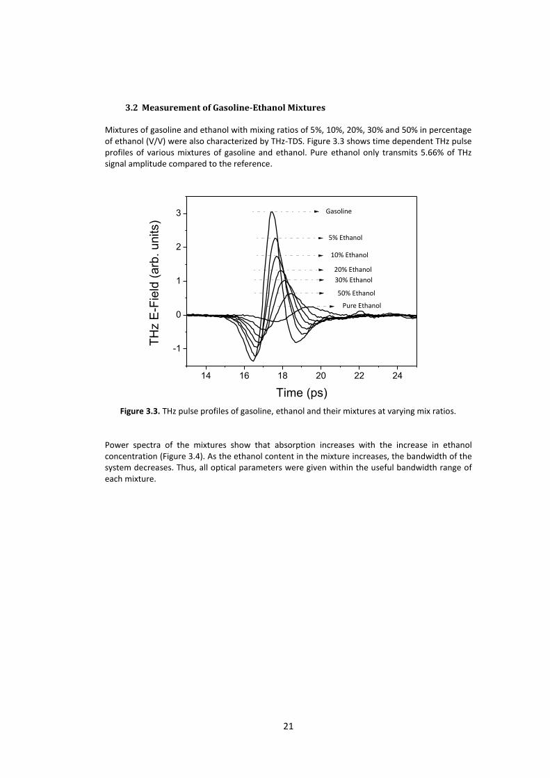
3.2 Measurement of Gasoline-Ethanol Mixtures

Mixtures of gasoline and ethanol with mixing ratios of 5%, 10%, 20%, 30% and 50% in percentage of ethanol (V/V) were also characterized by THz-TDS. Figure 3.3 shows time dependent THz pulse profiles of various mixtures of gasoline and ethanol. Pure ethanol only transmits 5.66% of THz signal amplitude compared to the reference.

14 16 18 20 22 24

-1

0

1

2

3

TH

z E

-Fie

ld (

arb

. units)

Time (ps)

Figure 3.3. THz pulse profiles of gasoline, ethanol and their mixtures at varying mix ratios. Power spectra of the mixtures show that absorption increases with the increase in ethanol concentration (Figure 3.4). As the ethanol content in the mixture increases, the bandwidth of the system decreases. Thus, all optical parameters were given within the useful bandwidth range of each mixture.

20% Ethanol

Gasoline

5% Ethanol

10% Ethanol

30% Ethanol

50% Ethanol

Pure Ethanol

22

0,2 0,4 0,6 0,8 1,0 1,210

-5

10-4

10-3

10-2

10-1

100

101

102

103

Gasoline

5%

10%

20%

30%

50%

Ethanol

Pow

er

(a.u

.)

Frequency (THz)

Figure 3.4. Power transmission spectra derived from Fast Fourier Transform of the data in Figure 3.3.

It is interesting to notice that the THz peak amplitude does not change linearly with the amount of ethanol added but rather exponentially decrease as the ethanol fraction increases (Figure 3.5a). However, a linear shift in time domain was observed as the ethanol concentration increases (Figure 3.5b).

23

0 20 40 60 80 1000,0

0,5

1,0

1,5

2,0

2,5

3,0

3,5

TH

z P

eak A

mplit

ude (

arb

. units)

Percent Ethanol

0 20 40 60 80 100

0,0

0,5

1,0

1,5

2,0

De

lay T

ime R

ela

tive T

o G

asolin

e (

ps)

Percent Ethanol

Figure 3.5. (a) Graph of THz peak amplitude vs. ethanol concentration. Cross symbols are experimental values, solid line is an exponential fitting. (b) Graph of delay time relative to

gasoline vs. percent ethanol. Star symbols are experimental data and solid line is a linear fitting.

(b)

(a)

24

Percent ethanol dependent delay time data in Figure 3.5b were fit to the linear equation below;

is the relative delay time in ps, is the percent ethanol. The parameters of the best fit resulted and for and , respectively. Percent ethanol dependent THz field amplitude data in Figure 3.5.a were fit to the exponential decay equation below;

where is the THz peak amplitude, is the percent ethanol, and are the fitting parameters. The parameters for the best fit were defined as Therefore, without a Fourier Transform of THz electric field, we are able to obtain two important information; percent ethanol dependent THz peak amplitude and relative delay time spectra. Fits were done in order to form a calibration curve which then can be used as a simple technique to estimate the amount of ethanol in a given gasoline-ethanol mixture. THz peak amplitude spectrum has maximum estimation error of 1.1% in terms of ethanol percentage, whereas relative delay time spectrum has maximum estimation error of 2.2%. To sum up, within a simple measurement we are able to predict the ethanol content in gasoline. In order to understand these mixture systems better, experimental results should be supported by theoretical modeling. Considering this, we further investigated the experimental data and modeling in the following sections.

3.2.1 Optical Properties of Mixtures The frequency dependent refractive index and absorption coefficient of mixtures derived from the THz transmission measurements are given in Figure 3.6.

25

0,2 0,4 0,6 0,8 1,0

1,45

1,50

1,55

1,60

1,65

1,70

1,75

1,80

1,85

Ethanol

50%

30%

20%

10%

5%

Gasol ine

Re

fra

ctive Index

Frequency (THz)

0,2 0,4 0,6 0,8 1,0

0

10

20

30

40

50

60 Ethanol

50%

30%

20%

10%

5%

Gasoline

Absorp

tion C

oeffic

ient (c

m-1)

Frequency (THz)

Figure 3.6. Comparison of frequency dependent refractive index (a) and absorption coefficient

(b) of gasoline-ethanol mixtures. The pure ethanol has higher refractive index at all frequencies. As the ethanol percentage decreases in the mixture, so does the refractive index of the mixtures as we expected since the pure gasoline has much lower refractive index at all frequencies. The absorption coefficient of pure ethanol is significantly higher than that of gasoline as we expected. Ethanol is a polar molecule which strongly absorbs THz waves more than gasoline due to the interaction of THz frequencies with the permanent dipole moment.

46 However, gasoline is mainly composed of non-

polar molecules.41

Thus the molecules in gasoline have transient dipole moment which causes

(a)

(b)

26

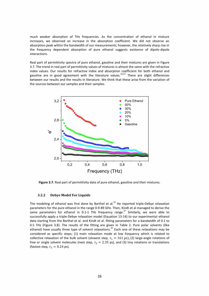
much weaker absorption of THz frequencies. As the concentration of ethanol in mixture increases, we observed an increase in the absorption coefficient. We did not observe an absorption peak within the bandwidth of our measurements; however, the relatively sharp rise in the frequency dependent absorption of pure ethanol suggests existence of dipole-dipole interactions. Real part of permittivity spectra of pure ethanol, gasoline and their mixtures are given in Figure 3.7. The trend in real part of permittivity values of mixtures is almost the same with the refractive index values. Our results for refractive index and absorption coefficient for both ethanol and gasoline are in good agreement with the literature values.

42,57 There are slight differences

between our results and the results in literature. We think that these arise from the variation of the sources between our samples and their samples.

0,2 0,4 0,6 0,8 1,0

2,0

2,4

2,8

3,2 Pure Ethanol

50%

30%

20%

10%

5%

Gasoline

e'

Frequency (THz)

Figure 3.7. Real part of permittivity data of pure ethanol, gasoline and their mixtures.

3.2.2 Debye Model For Liquids The modeling of ethanol was first done by Barthel et al.

52 He reported triple-Debye relaxation

parameters for the pure ethanol in the range 0.9-89 GHz. Then, Kindt et al managed to derive the same parameters for ethanol in 0.1-1 THz frequency range.

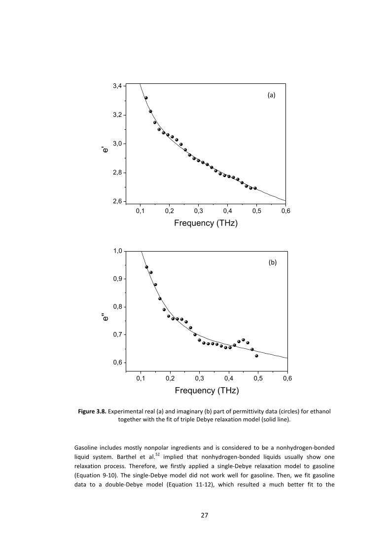
57 Similarly, we were able to

successfully apply a triple-Debye relaxation model (Equation 13-14) to our experimental ethanol data starting from the Barthel et al. and Kindt et al. fitting parameters for a bandwidth of 0.1 to 0.5 THz (Figure 3.8). The results of the fitting are given in Table 2. Pure polar solvents (like ethanol) have usually three type of solvent relaxations.

47 Each one of these relaxations may be

considered as specific steps; (1) main relaxation mode at low frequency which is related to collective relaxation of the bulk solvent (slowest step, (2) large-angle rotations of free or single solvent molecules (next step, ps), and (3) tiny rotations or translations (fastest step, ps).

27

0,1 0,2 0,3 0,4 0,5 0,6

2,6

2,8

3,0

3,2

3,4

e'

Frequency (THz)

0,1 0,2 0,3 0,4 0,5 0,6

0,6

0,7

0,8

0,9

1,0

e''

Frequency (THz)

Figure 3.8. Experimental real (a) and imaginary (b) part of permittivity data (circles) for ethanol

together with the fit of triple Debye relaxation model (solid line).

Gasoline includes mostly nonpolar ingredients and is considered to be a nonhydrogen-bonded

liquid system. Barthel et al.52

implied that nonhydrogen-bonded liquids usually show one

relaxation process. Therefore, we firstly applied a single-Debye relaxation model to gasoline

(Equation 9-10). The single-Debye model did not work well for gasoline. Then, we fit gasoline

data to a double-Debye model (Equation 11-12), which resulted a much better fit to the

(a)

(b)

28

experimental data (Figure 3.8). For gasoline the first relaxation was found as 3.18 ps ( , slow

relaxation) and the second relaxation ( , fast relaxation) was found as 0.045 ps. Since gasoline is

a mixture composed of many different compounds in unknown concentrations, it is hard to

define the relaxation states at this point.

0,2 0,4 0,6 0,8 1,0 1,22,04

2,07

2,10

2,13

e'

Frequency (THz)

0,2 0,4 0,6 0,8 1,0 1,2

0,03

0,06

0,09

0,12

0,15

e''

Frequency (THz)

Figure 3.9. Experimental real (a) and imaginary (b) part of permittivity data (circles) for gasoline together with the fit of double Debye relaxation model (solid line).

Calculated dielectric relaxation parameters of gasoline are also given in Table 3.1.

(a)

(b)

29

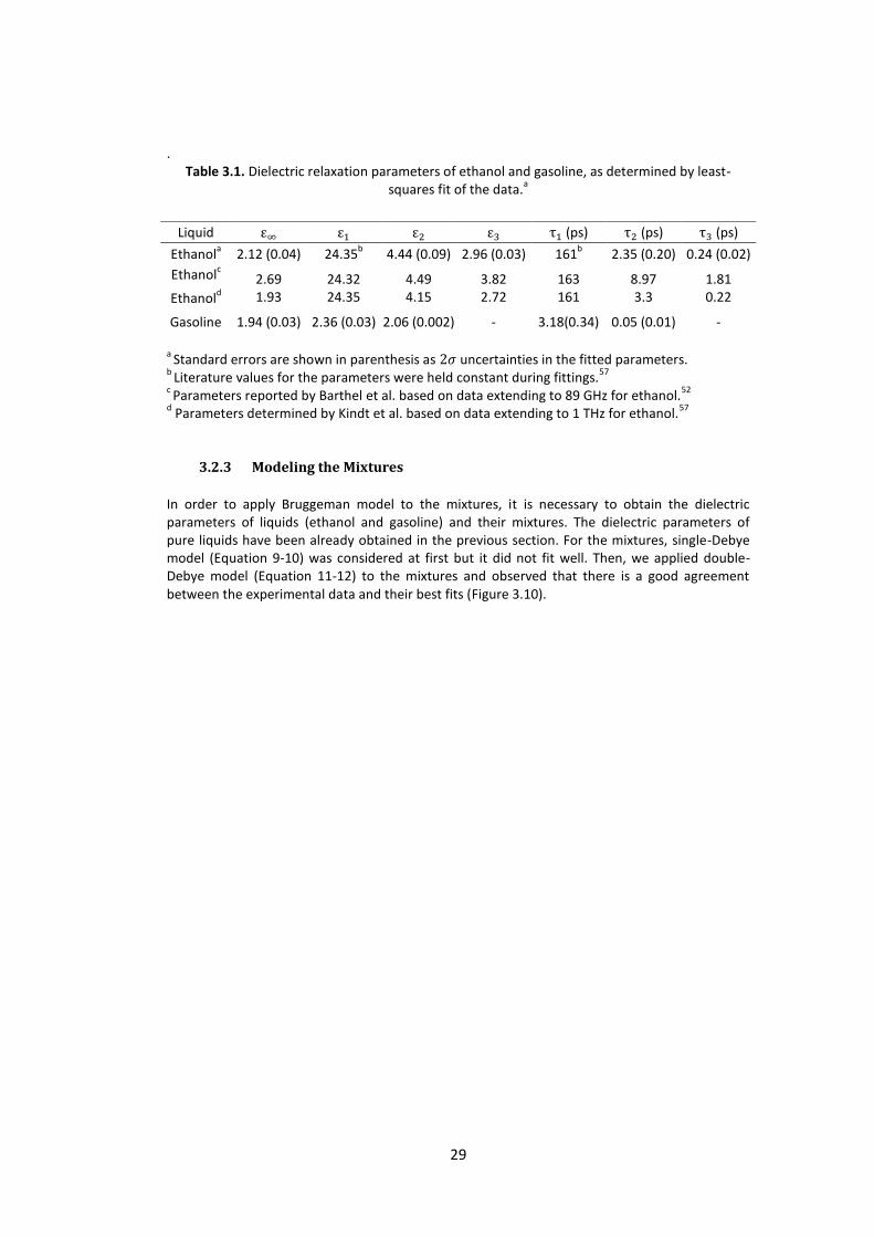
. Table 3.1. Dielectric relaxation parameters of ethanol and gasoline, as determined by least-

squares fit of the data.a

a Standard errors are shown in parenthesis as uncertainties in the fitted parameters.

b Literature values for the parameters were held constant during fittings.

57

c Parameters reported by Barthel et al. based on data extending to 89 GHz for ethanol.

52

d Parameters determined by Kindt et al. based on data extending to 1 THz for ethanol.

57

3.2.3 Modeling the Mixtures

In order to apply Bruggeman model to the mixtures, it is necessary to obtain the dielectric parameters of liquids (ethanol and gasoline) and their mixtures. The dielectric parameters of pure liquids have been already obtained in the previous section. For the mixtures, single-Debye model (Equation 9-10) was considered at first but it did not fit well. Then, we applied double-Debye model (Equation 11-12) to the mixtures and observed that there is a good agreement between the experimental data and their best fits (Figure 3.10).

Liquid (ps) (ps) (ps)

Ethanola 2.12 (0.04) 24.35

b 4.44 (0.09) 2.96 (0.03) 161

b 2.35 (0.20) 0.24 (0.02)

Ethanolc 2.69

1.93 24.32 24.35

4.49 4.15

3.82 2.72

163 161

8.97 3.3

1.81 0.22 Ethanol

d

Gasoline 1.94 (0.03) 2.36 (0.03) 2.06 (0.002) - 3.18(0.34) 0.05 (0.01) -

30

0,2 0,4 0,6 0,8 1,0 1,22,0

2,2

2,4

2,6

2,8

Percent Ethanol

50%

30%

20%

10%

5%

e'

Frequency (THz)

0,2 0,4 0,6 0,8 1,0 1,2

0,1

0,2

0,3

0,4

0,5

0,6

50%

30%

20%

10%

5%

e''

Frequency (THz)

Percent Ethanol

Figure 3.10. Experimental real (a) and imaginary (b) part of permittivity data (circles) for mixtures

of gasoline-ethanol together with the double-Debye relaxation model (solid line).

The dielectric parameters of mixtures were given in Table 3.2. At first, in order to analyze the

mixtures, we took a different approach in applying the Bruggeman model. After analyzing the

experimental results, we first modeled the mixture effective dielectric medium using a double-

Debye model as shown above and then calculated the corresponding Bruggeman factor.

Bruggeman factor ( ) was directly calculated by the dielectric constants of pure liquids (Table

3.1) and mixtures (Table 3.2) at zero frequency ( ) with equation 15. The initial analysis showed

that the Bruggeman factors did not scale with the volume concentration of ethanol. In order to

(a)

(b)

31

understand this behavior then, the calculated Bruggeman factors were fit by Equation 16. The

fitting parameter “ ” was determined by the least square fit method and it was found to be 0.36.

However, as it can be seen in Figure 3.11 the fit is not accurate. Therefore, it is very hard to

comment on the value of parameter “a” and its meaning in this analysis.

Table 3.2. Dielectric relaxation parameters of mixtures, as determined by least-squares fit of the

data.a

a Standard errors are shown in parenthesis as uncertainties in the fitted parameters.

Therefore, we concluded that Bruggeman model does not work for these mixtures. We also applied triple-Debye model (Equation 13-14) to determine the dielectric properties of the mixtures in order to obtain better Bruggeman factors. However, results were not better than the ones obtained from the double-Debye model.

0,0 0,2 0,4 0,6 0,8 1,0

0,0

0,2

0,4

0,6

0,8

1,0 Calculated

Ideal

Fit

f B

2

Figure 3.11. The Bruggeman plot for ethanol in gasoline. Black solid line is ideal behavior, Blue dots are calculated bruggeman factors and their fit is shown as red line.

Liquid (ps) (ps)

50% 2.07 (0.02) 3.55 (0.04) 2.52 (0.01) 2.16 (0.12) 0.20 (0.01)

30% 2.09 (0.01) 3.13 (0.04) 2.42 (0.01) 2.56 (0.20) 0.26 (0.01)

20% 2.05 (0.01) 2.78 (0.02) 2.29 (0.01) 1.78 (0.12) 0.19 (0.01)

10% 2.02 (0.004) 2.68 (0.02) 2.21 (0.004) 2.40 (0.16) 0.18 (0.01)

5% 2.05 (0.002) 2.37 (0.01) 2.18 (0.01) 1.59 (0.17) 0.27 (0.02)

32

3.2.4 Modified Debye Model For Mixtures The aim in this study is to find a simple but reliable technique in order to determine the volume fraction of ethanol content in gasoline. In the first approach, ethanol and gasoline interaction is ignored. Then, we further improved the second approach by considering a very weak interaction between ethanol and gasoline. Each approach was explained briefly and results were discussed in the following sections.

3.2.4.1 First Approach

In this method, we modeled the dielectric function of the mixtures with a basic contribution

approach (Equation 17) which is based on dissimilarities of the dielectric properties of ethanol

and gasoline. Ethanol is a polar molecule. However, gasoline is mainly composed of nonpolar

molecules.41

We assumed that interaction of molecules in gasoline and ethanol in the mixtures

are so weak that it can be ignored. Thus, the mixtures were modeled without any interaction

parameters in the function (Equation 17). Our second assumption is that A and B found from the

best fits of mixtures should be the fractions of ethanol and gasoline in mixture, respectively.

Therefore, the dielectric parameters found in pure ethanol and in gasoline from Table 3.1 were

directly used during the fitting process of the experimental data of the mixtures. Figure 3.12

shows the result of the fits to the experimental data and estimated content amounts (A and B)

are given in Table 3.3.

33

0,2 0,4 0,6 0,8 1,0 1,22,0

2,2

2,4

2,6

2,8

Percent Ethanol

50%

30%

20%

10%

5%

e'

Frequency (THz)

0,2 0,4 0,6 0,8 1,0 1,2

0,1

0,2

0,3

0,4

0,5

0,6

50%

30%

20%

10%

5%

e''

Frequency (THz)

Percent Ethanol

Figure 3.12. Experimental real (a) and imaginary (b) part of permittivity data (circles) for mixtures of gasoline-ethanol together with the improved Debye relaxation model (solid line).

(a)

(b)

34

Table 3.3. Parameters A and B (A+B≤1) (with standard errors in parenthesis) of mixtures. All the dielectric parameters were derived from the fit of pure ethanol and gasoline, and kept constant during the fitting process.

Variables 50% 30% 20% 10% 5%

(fraction) 0.54 (0.01) 0.36 (0.005) 0.25 (0.004) 0.16 (0.002) 0.08 (0.005)

(fraction) 0.46 (0.01) 0.64 (0.01) 0.75 (0.01) 0.84 (0.002) 0.92 (0.01)

Values of A are shown as red circle scatters with line and expected values of A are shown as black line in Figure 3.13. For all the mixtures, the estimated ethanol contents (A) were found to be higher than the experimental ones (the amounts used for mixing), while the gasoline contents (B) were found to be lower. The modeled system for detection of ethanol content in gasoline works adequately with respect to our assumptions. In order to obtain better estimations, we considered weak interactions between the ethanol and gasoline molecules which is explained in detail in the following section.

0 20 40 60 80 100

0,0

0,2

0,4

0,6

0,8

1,0

A

Percent Ethanol

Figure 3.13. Values of A (red circles) found from the best fits of the mixtures’ data. Black line is

experimental values of A.

3.2.4.2 Second Approach The results of first approach led us to think on the possibility of the weak interactions between

the ethanol and the low-polarizable molecules in gasoline. These interactions were assumed to

have impact on relaxations of ethanol and gasoline. We think that these weak interactions should

have a stronger impact more on the fastest relaxation steps rather than the slower ones.

Therefore, the parameters that are corresponding to the fastest relaxation

35

were allowed to change while others were held fixed during the fitting process (Equation 17). In

such a multi-parameter fitting process, allowing all the parameters to change at once does not

work well. Thus fittings were started by keeping all the parameters (except A and B) fixed to their

derived values from the ethanol and gasoline (first approach). Then, the dielectric parameters

were allowed to change one by one, iteratively until the fitting converged.

The results are shown in Figure 3.14. For each mixture, there is a good agreement between the

experimental data and their best fits. Furthermore, fits are much better than the previous

method when both the residual and regression values are compared. The resultant fit

parameters are given in Table 3.4. The derived values of the composition parameters A and B are

very close to their expected values.

36

0,2 0,4 0,6 0,8 1,0 1,22,0

2,2

2,4

2,6

2,8

Percent Ethanol

50%

30%

20%

10%

5%

e'

Frequency (THz)

0,2 0,4 0,6 0,8 1,0 1,2

0,1

0,2

0,3

0,4

0,5

0,6Percent Ethanol

50%

30%

20%

10%

5%

e''

Frequency (THz)

Figure 3.14. The improved Debye relaxation model (solid line) along with the real (a) and

imaginary (b) part of permittivity data (circles) derived from the experimental measurements for the mixtures of ethanol and gasoline.

(a)

(b)

37

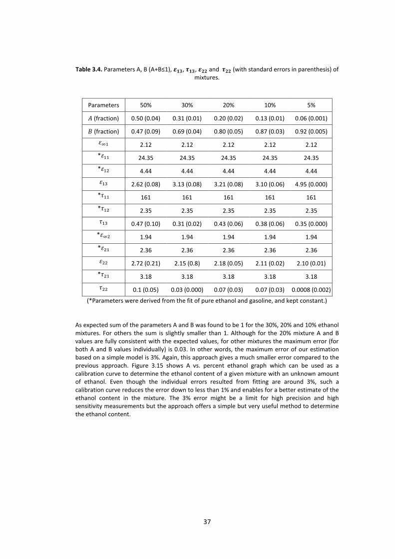
Table 3.4. Parameters A, B (A+B≤1), , , and (with standard errors in parenthesis) of mixtures.

Parameters 50% 30% 20% 10% 5%

(fraction) 0.50 (0.04) 0.31 (0.01) 0.20 (0.02) 0.13 (0.01) 0.06 (0.001)

(fraction) 0.47 (0.09) 0.69 (0.04) 0.80 (0.05) 0.87 (0.03) 0.92 (0.005)

2.12 2.12 2.12 2.12 2.12

* 24.35 24.35 24.35 24.35 24.35

* 4.44 4.44 4.44 4.44 4.44

2.62 (0.08) 3.13 (0.08) 3.21 (0.08) 3.10 (0.06) 4.95 (0.000)

* 161 161 161 161 161

* 2.35 2.35 2.35 2.35 2.35

0.47 (0.10) 0.31 (0.02) 0.43 (0.06) 0.38 (0.06) 0.35 (0.000)

* 1.94 1.94 1.94 1.94 1.94

* 2.36 2.36 2.36 2.36 2.36

2.72 (0.21) 2.15 (0.8) 2.18 (0.05) 2.11 (0.02) 2.10 (0.01)

* 3.18 3.18 3.18 3.18 3.18

0.1 (0.05) 0.03 (0.000) 0.07 (0.03) 0.07 (0.03) 0.0008 (0.002)

(*Parameters were derived from the fit of pure ethanol and gasoline, and kept constant.) As expected sum of the parameters A and B was found to be 1 for the 30%, 20% and 10% ethanol mixtures. For others the sum is slightly smaller than 1. Although for the 20% mixture A and B values are fully consistent with the expected values, for other mixtures the maximum error (for both A and B values individually) is 0.03. In other words, the maximum error of our estimation based on a simple model is 3%. Again, this approach gives a much smaller error compared to the previous approach. Figure 3.15 shows A vs. percent ethanol graph which can be used as a calibration curve to determine the ethanol content of a given mixture with an unknown amount of ethanol. Even though the individual errors resulted from fitting are around 3%, such a calibration curve reduces the error down to less than 1% and enables for a better estimate of the ethanol content in the mixture. The 3% error might be a limit for high precision and high sensitivity measurements but the approach offers a simple but very useful method to determine the ethanol content.

38

0 20 40 60 80 100

0,0

0,2

0,4

0,6

0,8

1,0

A

Percent Ethanol

Figure 3.15. Values of A (red circles) found from the best fits of the mixtures’ data. Black line is

experimental values of A. The errors are possibly a combination of both systematic and measurement errors. Small fluctuations in temperature and humidity in the environment affect THz measurements since the optics and electronics used in the spectrometer and the laser source are very sensitive to the changes in temperature and humidity. In addition, measurement errors may have occurred during the preparation of the solutions. 20 mL of solutions were prepared for each mixture. The smallest volume that the pipette can measure is 0.1 mL. Thus, the measurement error is in the order of 0.05 mL on that pipette. For a 5 mL liquid measurement this corresponds to a maximum error of 1%. Although the error only from the sample preparation looks small, when it is combined with the instrumental error, its effect on the results may become significant. It is possible to conduct more precise measurements by minimizing these systematic and measurement errors and also by increasing the signal-to-noise ratio of the instrument.

39

CHAPTER 4

CONCLUSIONS

In this study, a new method for the detection of ethanol in gasoline was presented by using THz-TDS technique. For this purpose, a THz-TDS system was constructed for the measurements of fuel oils and their ethanol mixtures. In this system, photoconductive antenna was used for the generation of THz and a 2 mm thickness ZnTe electro-optic crystal was used for the detection of THz. The bandwidth of the instrument was determined as 0.1-1.6 THz with 10

4 S/N ratio.

Fuel oil samples (diesel and gasoline) were probed by THz waves and their optical properties were determined. Diesel has higher refractive index than gasoline. However, absorption coefficient of diesel was found to be lower than that of gasoline. Differences in both frequency dependent refractive index and absorption coefficient are caused by the variation in compositions of the ingredients in gasoline and diesel. We did not observe any absorption peaks within the bandwidth of our measurements. Real part of permittivity of fuel oils was also calculated and presented. It was shown that qualitative analysis of fuel oils could be done by comparing optical parameters obtained by THz-TDS technique. Pure ethanol, gasoline and their mixtures were measured by THz-TDS. Optical parameters were presented such as absorption coefficient, refractive index and real part of permittivity. Ethanol has higher refractive index and absorption coefficient than that of gasoline. Therefore, addition of ethanol to the mixture causes an increase in both refractive index and absorption coefficient. Optical parameters of ethanol and gasoline are in good agreement with the literature values. We did not observe an absorption peak within the bandwidth of our measurements; however, the relatively sharp rise in the frequency dependent absorption of pure ethanol suggests existence of dipole-dipole interactions. Percent ethanol dependent THz peak amplitude and relative delay time spectra were calculated. Then, these were fit to exponential decay and linear equations, respectively; that could be considered as calibration curves with their best fits. The results show that even with such a simple approach, obtained calibration curves can be used as an estimation method of ethanol content in a given gasoline-ethanol mixture with an accuracy of 1.1% for the peak amplitude comparison and 2.2% for the relative delay time due to the refractive index change. For a better understanding of these mixture systems, experimental data were further investigated by theoretical modeling. Debye model is used for modeling the complex dielectric permittivity function of pure liquids. In this study, pure ethanol data was modeled with a triple-Debye model as in the literature. It was shown that the fit parameters are in good agreement with the ones reported in literature. For gasoline, double-Debye model was applied successfully. It is hard to define the relaxation states of gasoline, since it is a mixture composed of many different compounds in unknown concentrations. For the mixture modeling, we applied Bruggeman model first but the results were not satisfactory. Then, we constructed a simple model derived from Debye model considering basic contribution approach. In the first approach to model mixtures, ethanol and gasoline interaction was ignored. Then we further improved the model by considering a weak interaction between ethanol and gasoline. The second approach resulted in better fits compared to the first one. The maximum error based on the second approach is ca. 3%. This approach offers a simple and useful method to determine the ethanol content. For future work, in gasoline-ethanol mixtures, it may be possible to conduct a more precise measurement by minimizing systematic and measurement errors.

40

41

REFERENCES (1) Zhang, X. Introduction to Thz Wave Photonics; Springer, 2010. (2) Wiltse, J. C. IEEE Transactions on Microwave Theory and Techniques 1984, 32, 1118 –

1127. (3) Palik, E. D. Journal of the Optical Society of America 1977, 67, 857–865. (4) Sakai, K.; Joho Tsushin Kenkyu Kiko (Japan) Terahertz optoelectronics; Springer ; NiCT,

National Institute of Information and Communications Technology: Berlin; New York; [Tokyo], 2005.

(5) Auston, D. H.; Cheung, K. P.; Smith, P. R. Applied Physics Letters 1984, 45, 284 –286. (6) Smith, P. R.; Auston, D. H.; Nuss, M. C. IEEE Journal of Quantum Electronics 1988, 24, 255

–260. (7) Yajima, T.; Takeuchi, N. Japanese Journal of Applied Physics 1971, 10, 907–915. (8) Yang, K. H.; Richards, P. L.; Shen, Y. R. Applied Physics Letters 1971, 19, 320–323. (9) Schmuttenmaer, C. A. Chemical reviews 2004, 104, 1759–1779. (10) Mittleman, D. Sensing with terahertz radiation; Springer Verlag: Berlin, 2010. (11) Withayachumnankul, W.; Fischer, B. M.; Abbott, D. Proceedings of the Royal Society A:

Mathematical, Physical and Engineering Science 2008, 464, 2435–2456. (12) Yomogida, Y.; Sato, Y.; Yamakawa, K.; Nozaki, R.; Mishina, T.; Nakahara, J. Journal of

Molecular Structure 2010, 970, 171–176. (13) Arbab, M. H.; Winebrenner, D. P.; Thorsos, E. I.; Chen, A. Applied Physics Letters 2010, 97,

181903–181903–3. (14) Foltynowicz, R. J.; Allman, R. E.; Zuckerman, E. Chemical Physics Letters 2006, 431, 34–38. (15) Chakraborty, A.; Inagaki, T.; Banno, M.; Mochida, T.; Tominaga, K. The Journal of Physical

Chemistry A 2011, 115, 1313–1319. (16) Yamamoto, K.; Tani, M.; Hangyo, M. The Journal of Physical Chemistry. B 2007, 111,

4854–4859. (17) Zhao, G.; Wang, H.; Liu, L.; Wang, X. Science China Information Sciences 2012, 55, 114–

119. (18) Hua, Y.; Zhang, H. IEEE Transactions on Microwave Theory and Techniques 2010, 58, 2064

–2070. (19) Zheng, Z.-P.; Fan, W.-H.; Liang, Y.-Q.; Yan, H. Optics Communications 2012, 285, 1868–

1871. (20) Zheng, Z.-P.; Fan, W.-H.; Yan, H. Chemical Physics Letters 2012, 525–526, 140–143. (21) Markelz, A. G. IEEE Journal of Selected Topics in Quantum Electronics 2008, 14, 180 –190. (22) Yamamoto, K.; Yamaguchi, M.; Miyamaru, F.; Tani, M.; Hangyo, M.; Ikeda, T.; Matsushita,

A.; Koide, K.; Tatsuno, M.; Minami, Y. Japanese Journal of Applied Physics 2004, 43, L414–L417.

(23) Witko, E. M.; Korter, T. M. The Journal of Physical Chemistry A 2012, 116, 6879–6884. (24) Meng, K.; Li, Z.; Liu, Q. Guang Pu Xue Yu Guang Pu Fen Xi 2011, 31, 1305–1308. (25) Burton, M. G. Astronomy and Astrophysics Review 2010, 18, 417–469. (26) Federici, J.; Moeller, L. Journal of Applied Physics 2010, 107, 111101–111101–22. (27) Federici, J. F.; Schulkin, B.; Huang, F.; Gary, D.; Barat, R.; Oliveira, F.; Zimdars, D.

Semiconductor Science and Technology 2005, 20, S266–S280. (28) Smith, R. M.; Arnold, M. A. Applied Spectroscopy Reviews 2011, 46, 636–679. (29) Baxter, J. B.; Guglietta, G. W. Analytical Chemistry 2011, 83, 4342–4368. (30) Lane, P. A.; Cunningham, P. D.; Melinger, J. S.; Kushto, G. P.; Esenturk, O.; Heilweil, E. J.

Physical review letters 2012, 108, 077402. (31) Key World Energy Statistics; International Energy Agency, 2011; p.

http://www.iea.org/textbase/nppdf/free/2011/key_world_energy_stats.pdf. (32) A.D. Mohammed; I.A. Mohammed; C. S. Ajinomoh Journal of Innovative Research in

Engineering and Science 2011, 137–147.

42

(33) Wen, L.; Xin, C.-Y.; Yang, S.-C. Applied Energy 2010, 87, 115–121. (34) Al-Hasan, M. Energy Conversion and Management 2003, 44, 1547–1561. (35) USA Environmental Protection Agency

http://content.usatoday.com/communities/driveon/post/2010/10/epa-to-allow-15-ethanol-in-gasoline-up-from-10-%20now-/1#.URa3UaU02Sq (accessed Feb 9, 2013).

(36) Department of the Environment, Community & Local Government http://www.environ.ie/en/Environment/Atmosphere/AirQuality/FuelStandards/ (accessed Feb 9, 2013).

(37) Turkey Energy Community Regulatory Board http://www.resmigazete.gov.tr/eskiler/2012/07/20120707-35.htm (accessed Feb 9, 2013).

(38) Chung, H. Applied Spectroscopy Reviews 2007, 42, 251–285. (39) Kelly, J. J.; Callis, J. B. Analytical Chemistry 1990, 62, 1444–1451. (40) Fodor, G. E.; Kohl, K. B.; Mason, R. L. Analytical Chemistry 1996, 68, 23–30. (41) Al-Douseri, F. M.; Chen, Y.; Zhang, X.-C. International Journal of Infrared and Millimeter

Waves 2007, 27, 481–503. (42) Jin, Y.-S.; Kim, G.-J.; Shon, C.-H.; Jeon, S.-G.; Kim, J.-I. Journal of the Korean Physical

Society 2008, 53, 1879–1885. (43) Kim, G.-J.; Jeon, S.-G.; Kim, J.-I.; Jin, Y.-S. In 33rd International Conference on Infrared,

Millimeter and Terahertz Waves, 2008. IRMMW-THz 2008; 2008; pp. 1 –2. (44) Ahmed, M. K.; Levenson, J. Petroleum Science and Technology 2012, 30, 115–121. (45) Kindt, J. T.; Schmuttenmaer, C. A. The Journal of Physical Chemistry 1996, 100, 10373–

10379. (46) Keiding, S. R. The Journal of Physical Chemistry A 1997, 101, 5250–5254. (47) Asaki, M. L. T.; Redondo, A.; Zawodzinski, T. A.; Taylor, A. J. The Journal of Chemical

Physics 2002, 116, 8469–8482. (48) Siddhart P. Kamble; Sudake Y.S.; Patil S.S.; Khirade P.W.; Mehrotra S.C. International

Journal of Pharma and Bio Sciences 2011, 2, 297–306. (49) Patil A.V.; Achole B.D.; Shinde G.N.; Pawar V.P. Scholars Research Library 2012, 4, 1665–

1669. (50) BATOP GmbH http://www.batop.de/ (accessed Jan 11, 2013). (51) Dexheimer, S. L. Terahertz Spectroscopy: Principles and Applications; Taylor & Francis,

2007. (52) Barthel, J.; Buchner, R. Pure and Applied Chemistry 1991, 63, 1473–1482. (53) Cole, K. S.; Cole, R. H. The Journal of Chemical Physics 1941, 9, 341–351. (54) Cole, K. S.; Cole, R. H. The Journal of Chemical Physics 1942, 10, 98–105. (55) Davidson, D. W.; Cole, R. H. The Journal of Chemical Physics 1950, 18, 1417–1417. (56) Davidson, D. W.; Cole, R. H. The Journal of Chemical Physics 1951, 19, 1484–1490. (57) Kindt Journal of Physical Chemistry 1996, 100, 10373–10379. (58) Glancy, P.; Beyermann, W. P. The Journal of Chemical Physics 2010, 132, 245102. (59) Tübitak

http://biltek.tubitak.gov.tr/merak_ettikleriniz/index.php?kategori_id=4&soru_id=2976 (accessed Feb 9, 2013).