differentiable piecewise-bézier interpolation on ... · differentiable piecewise-bézier...

Differentiable piecewise-Bezier interpolation onRiemannian manifolds

P.-A. Absil1, Pierre-Yves Gousenbourger1,Paul Striewski2 and Benedikt Wirth2 ∗

1- Universite catholique de Louvain - ICTEAM InstituteB-1348 Louvain-la-Neuve, Belgium

2- University of Munster - Institute for Numerical and Applied MathematicsEinsteinstraße 62, D-48149 Munster, Germany

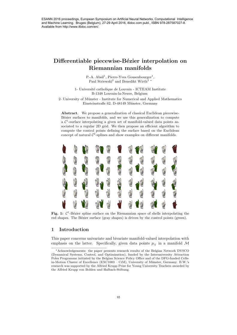
Abstract. We propose a generalization of classical Euclidean piecewise-Bezier surfaces to manifolds, and we use this generalization to computea C1-surface interpolating a given set of manifold-valued data points as-sociated to a regular 2D grid. We then propose an efficient algorithm tocompute the control points defining the surface based on the Euclideanconcept of natural C2-splines and show examples on different manifolds.

Fig. 1: C1-Bezier spline surface on the Riemannian space of shells interpolating thered shapes. The Bezier surface (gray shapes) is driven by the control points (green).

1 Introduction

This paper concerns univariate and bivariate manifold-valued interpolation withemphasis on the latter. Specifically, given data points pij in a manifold M

∗Acknowledgements: the paper presents research results of the Belgian Network DYSCO(Dynamical Systems, Control, and Optimization), funded by the Interuniversity AttractionPoles Programme initiated by the Belgian Science Policy Office and of the DFG-funded Cells-in-Motion Cluster of Excellence (EXC1003 – CiM), University of Munster, Germany. B.W.’sresearch was supported by the Alfried Krupp Prize for Young University Teachers awarded bythe Alfried Krupp von Bohlen und Halbach-Stiftung.

95

ESANN 2016 proceedings, European Symposium on Artificial Neural Networks, Computational Intelligence and Machine Learning. Bruges (Belgium), 27-29 April 2016, i6doc.com publ., ISBN 978-287587027-8. Available from http://www.i6doc.com/en/.

associated to nodes (i, j) ∈ Z2 of a Cartesian grid in R

2, we seek a C1 functionB : R2 →M such that B(i, j) = pij .

Several applications motivate this problem, such as projection-based modelorder reduction of a dynamical system depending on few parameters (whereMis a Grassmann manifold) [1] or upsampling of diffusion tensor images (whereM is the manifold of positive definite matrices) [2].

In contrast with the univariate case, multivariate manifold-valued interpo-lation does not appear much in the literature (see [3] and references therein).Steinke et al. [4, 5] use a thin-plate-spline technique to produce an interpolationmap between two Riemannian manifolds. We also mention a related techniquefor volumetric registration presented in [6]. WhenM = R

r, on the other hand,there is a wealth of methods, in particular those based on Bezier splines [7].

In this work, we interpolate the data points by means of C1 piecewise-cubicBezier surfaces (see Figure 1 for an example). First, we recall a bivariate exten-sion [3] of manifold-valued Bezier curves [8, 9, 10]. We also give a condition tomatch two Bezier patches C0-continuously and then present a slight modificationof the Bezier surface definition to ensure C1-continuity (Section 2). In Section 3we provide a technique to generate Bezier control points for interpolation whichis faster than in [3], and we present numerical examples in Section 4.

2 Reminder on piecewise-Bezier curves and surfaces

Bezier curves and surfaces of degree K ∈ N are functions of the form

βK(·; b0, . . . , bK) : [0, 1]→ Rr, t �→∑K

j=0 bjBjK(t),

βK(·, ·; (bij)i,j=0,...,K) : [0, 1]2 → Rr, (t1, t2) �→

∑Ki,j=0 bijBiK(t1)BjK(t2),

where BjK(t) =(

Kj

)

tj(1−t)K−j are Bernstein polynomials. They are parameter-

ized by control points b0, . . . , bK ∈ Rr (resp. (bij)i,j=0,...,K ⊂ R

r) which indicatethe rough shape of the curve or surface and which are interpolated when theirindices are in {0,K}.

Since Bernstein polynomials form a partition of unity, Bezier functions are ac-tually convex combinations of their control points. Introducing the weighted av-erage av[(y1, . . . , yn), (w1, . . . , wn)] = argminy

∑ni=1 wid

2(yi, y) with Euclideandistance d, an equivalent definition of the functions is

βK(t; b0, . . . , bK) = av[(bi)i=0,...,K , (BiK(t))i=0,...,K ],

βK(t1, t2; (bij)i,j=0,...,K) = av[(bij)i,j=0,...,K , (BiK(t1)BjK(t2))i,j=0,...,K ]. (1)

This definition has the advantage that it generalizes to arbitrary metric spaces.In particular, this is one way among others to define Bezier functions on aRiemannian manifoldM [3].

LetM be a Riemannian manifold (the special caseM = Rr is included). A

piecewise-Bezier curve is defined by patching multiple Bezier curves together as

B : [0,M ]→M, t �→ βK(t−m; (bmi )i=0,...,K) on [m,m+ 1],

96


for m ∈ {0, . . . ,M − 1}, and accordingly for surfaces B : [0,M ]×[0, N ] → M.These piecewise-Bezier curves are continuous if bm−1

K = bm0 , m = 1, . . . ,M − 1.

The surfaces are continuous if bm,n−1iK = bmn

i0 for all i ∈ {0, . . . ,K} and (m,n) ∈{0, . . . ,M − 1} × {1, . . . , N − 1}, and accordingly in the other direction [3].

If we additionally desire continuous differentiability, then in Euclidean spacethis leads to a set of additional simple constraints on the control points [7]. Forpiecewise-Bezier surfaces, if we allow also indices outside {0, . . . ,K} by setting

bmn−1,j = bm−1,n

K−1,j , bmnK+1,j = bm+1,n

1,j , bmnj,−1 = bm,n−1

j,K−1 , bmnj,K+1 = bm,n+1

j,1 ,

the C1-conditions become bmni0 =

bmni,−1+bmn

i1

2 and bmn0j =

bmn−1,j+bmn

1j

2 for all i, j,m, n.Unfortunately, it turns out that those constraints cannot be generalized to aRiemannian manifold M without leading to contradictions [3]. Therefore, toachieve a C1 piecewise Bezier surface in M, one has to slightly alter the defi-nition of a Bezier surface. Indeed, the Euclidean C1-conditions imply that allcontrol points bmn

i0 and bmn0j can be ignored and replaced by the average of their

neighbors. Thus, with I = {−1, 1, 2, . . . ,K − 1,K + 1}, one redefines [3]

βK(t1, t2; (bmnij )i,j=0,...,K) = av

[

(bmnij )i,j∈I , (wi(t1)wj(t2))i,j∈I

]

(2)

with weights wi(t) =

⎧

⎪

⎪

⎪

⎪

⎪

⎪

⎨

⎪

⎪

⎪

⎪

⎪

⎪

⎩

12B0K(t) if i = −1,B1K(t) + 1

2B0K(t) if i = 1,

BiK(t) if i = 2, . . . ,K − 2,

BK−1,K(t) + 12BKK(t) if i = K − 1,

12BKK(t) if i = K + 1.

For C1 piecewise Bezier surfaces in Euclidean space, (2) is equivalent to (1).

3 Efficient control point generation for 1D and 2D piecewise-cubic Bezier interpolation on manifolds

Consider data points pmn ∈ M, (m,n) ∈ {0, . . . ,M} × {0, . . . , N}, where Mis a connected, smooth, finite-dimensional manifold, and where the points arenot too far from each other so that their weighted averages are well-defined. Tointerpolate those with a C1-continuous piecewise-cubic (K = 3) Bezier surfaceB : [0,M ]× [0, N ]→M with B(m,n) = pmn, we need to generate appropriatecontrol points

bmnij for m,n ∈ {0, . . . ,M − 1} × {0, . . . , N − 1} and i, j = 1, 2.

Note that in view of (2), only inner control points bmnij need to be computed.

Curves. To find an appropriate method, we first consider the Euclidean spaceR

r and examine piecewise-Bezier curves. Given points pm in Rr, there exists a

97


unique C2-interpolating piecewise-cubic Bezier curve B whose second derivativein normal direction vanishes at the domain boundary [7, §9.3]. As a furthernice characteristic, this piecewise-Bezier curve additionally minimizes the mean

squared acceleration∫M

0‖B′′(t)‖2dt among all interpolating curves [7, §9.5].

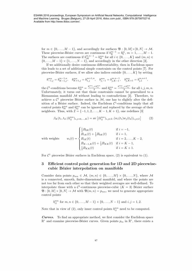
Consider the B-spline representation of this optimal curve,B =∑M+1

m=−1αmBm,with coefficients α−1, . . . , αM+1 ∈ R

r and with Bm = B(· −m) given by

−2 −1 1 2

–1/6–1/3

2/3

B(t) =

⎧

⎪

⎪

⎪

⎪

⎪

⎪

⎨

⎪

⎪

⎪

⎪

⎪

⎪

⎩

β3(t+ 2; 0, 0, 0, 16 ) if t ∈ [−2,−1],β3(t+ 1; 1

6 ,13 ,

23 ,

23 ) if t ∈ [−1, 0],

β3(t− 0; 23 ,

23 ,

13 ,

16 ) if t ∈ [0, 1],

β3(t− 1; 16 , 0, 0, 0) if t ∈ [1, 2],

0 else.

(3)

The constraints B(m) = pm and B′′(0) = B′′(M) = 0 result in the linear system

1

6

(

4 1

1...

......

... 11 4

)

︸︷︷︸

=:AM

(

α1...

αM−1

)

=

⎛

⎜

⎝

p1−p0

6p2...

pM−2

pM−1−pM

6

⎞

⎟

⎠

︸︷︷︸

=:PM (p0,...,pM )

,α0 = p0 ,αM = pM ,α−1 = 2α0 − α1 ,

αM+1 = 2αM − αM−1 .

Finally, inserting (3) intoB =∑M+1

m=−1 αmB(·−m) we see that the Bezier controlpoints bmj can be computed as

bm0 = pm, bm1 = 23αm + 1

3αm+1, bm2 = 13αm + 2

3αm+1, bm3 = pm+1 .

Surfaces. Consider now the optimal interpolating piecewise-cubic Bezier sur-face B, still in R

r. Its B-spline representation is B =∑M+1

m=−1

∑N+1n=−1 αmnBmn

with Bmn(t1, t2) = Bm(t1)Bn(t2). Since those basis elements are just ten-sorised versions of the univariate case, a natural way to find the coefficientsαmn ∈ R

r is to first identify the coefficients of the N + 1 spline curves inter-polating p0n, . . . , pMn, n = 0, . . . , N , and then interpret those coefficients asinterpolation points for spline curves along the other dimension. In detail, theproblem to solve is now

α0n=p0n, αMn=pMn, AM(α1n, . . . , αM−1,n)T =PM (p0n, . . . , pMn) ∀n,

α0n= αm0, αMn= αmN , AN(αm1, . . . , αm,N−1)T =PN (αm0, . . . , αmN ) ∀m.

An equivalent method is the following: first, compute intermediate points

pmn = P(p,m, n) = PMm

(

PNn (p00, . . . , p0N ), . . . , PN

n (pM0, . . . , pMN ))

(4)

for all (m,n); then, denoting A = A−1, the αmn are given by

αmn = A(p,m, n) =M∑

i=1

N∑

j=1

AMmiA

Nnj pij . (5)

98


Note that the entries of AM and AN decay exponentially away from the diagonal.Choosing a small d ∈ N and allowing a small error, the optimal coefficients arethus approximated as αmn = ′∑m+d

i=m−d′∑n+d

j=n−d AMmiA

Nnj pij , where ′∑ is a

summation restricted to indices for which the summands are defined.Finally, the Bezier control points bmn

ij for i, j ∈ {1, 2} are obtained via

bmnij = 3−i

33−j3 αmn + 3−i

3j3αm,n+1 +

i33−j3 αm+1,n + i

3j3αm+1,n+1.

Manifold setting. To generalize the approach to a Riemannian manifoldM,we observe that the equations stay valid under translations, that is, if we replaceall αmn and pmn by respectively αmn = αmn − pref and pmn = pmn − pref . Insummary, we compute pmn = P(p,m, n) and then obtain αmn = A(p,m, n).

On a Riemannian manifoldM, we interpret the Euclidean difference a−prefas a “projection” of a on the tangent space at pref . Namely, we replace alldifferences by logarithms logpref

a. In the computation of αmn = logprefαmn

one should choose pref = pmn as the closest interpolation point. The choice of asmall d now has the advantage that the computation requires only few logarithmslogpref

pmn which are typically expensive to obtain and form the numerical bot-tleneck of the approach. At the end, αmn ∈M is retrieved as αmn = exppmn

αmn

and the control points for i, j ∈ {1, 2} as

bmnij = av[(αmn, αm,n+1, αm+1,n, αm+1,n+1), (

3−i3

3−j3 , 3−i

3j3 ,

i33−j3 , i

3j3 )] .

4 Numerical examples

We present here some examples of piecewise-Bezier surfaces computed on thesphere, the orthogonal group and the space of shells, with d = 1.

Figure 2a shows a result on S2 where well-known explicit formulas for log-

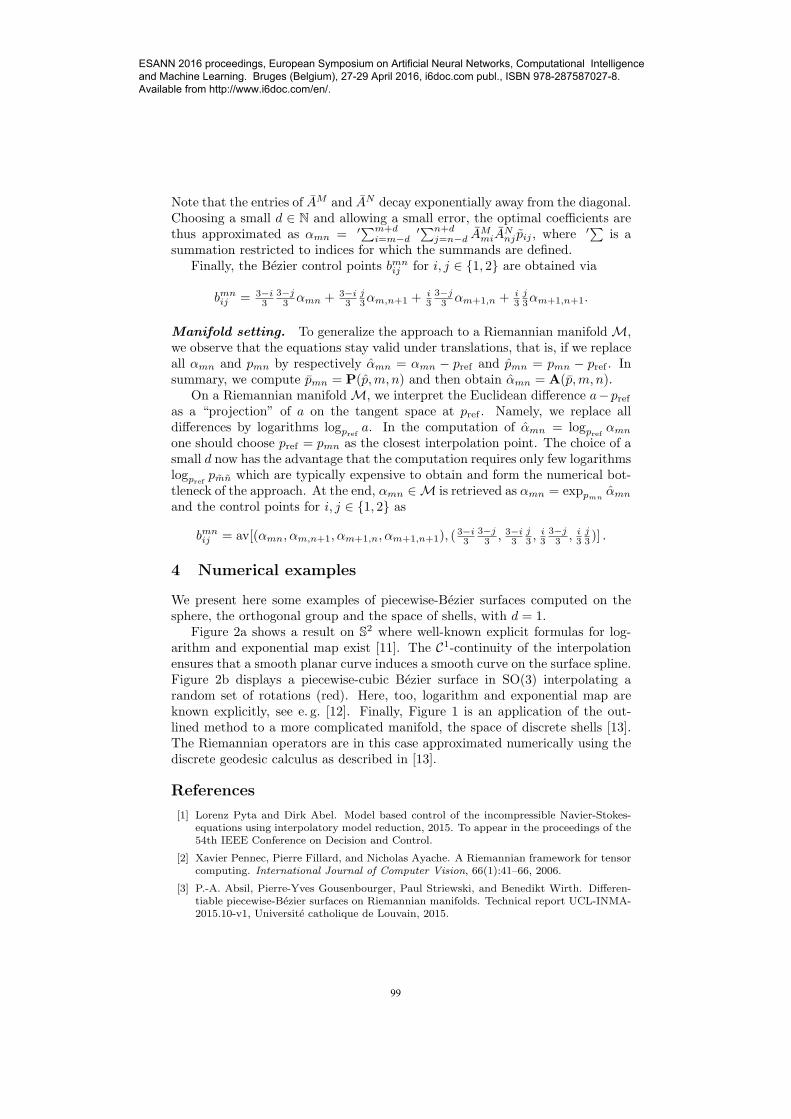
arithm and exponential map exist [11]. The C1-continuity of the interpolationensures that a smooth planar curve induces a smooth curve on the surface spline.Figure 2b displays a piecewise-cubic Bezier surface in SO(3) interpolating arandom set of rotations (red). Here, too, logarithm and exponential map areknown explicitly, see e. g. [12]. Finally, Figure 1 is an application of the out-lined method to a more complicated manifold, the space of discrete shells [13].The Riemannian operators are in this case approximated numerically using thediscrete geodesic calculus as described in [13].

References

[1] Lorenz Pyta and Dirk Abel. Model based control of the incompressible Navier-Stokes-equations using interpolatory model reduction, 2015. To appear in the proceedings of the54th IEEE Conference on Decision and Control.

[2] Xavier Pennec, Pierre Fillard, and Nicholas Ayache. A Riemannian framework for tensorcomputing. International Journal of Computer Vision, 66(1):41–66, 2006.

[3] P.-A. Absil, Pierre-Yves Gousenbourger, Paul Striewski, and Benedikt Wirth. Differen-tiable piecewise-Bezier surfaces on Riemannian manifolds. Technical report UCL-INMA-2015.10-v1, Universite catholique de Louvain, 2015.

99


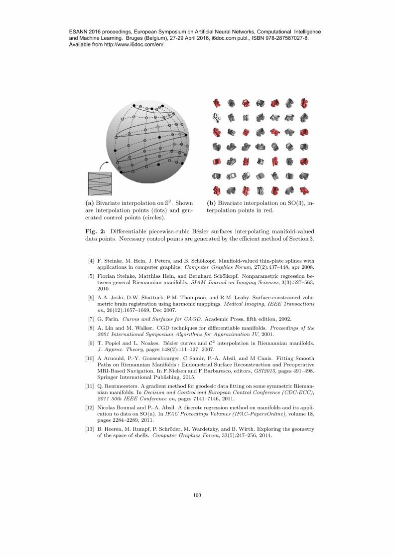
(a) Bivariate interpolation on S2. Shown

are interpolation points (dots) and gen-erated control points (circles).

(b) Bivariate interpolation on SO(3), in-terpolation points in red.

Fig. 2: Differentiable piecewise-cubic Bezier surfaces interpolating manifold-valueddata points. Necessary control points are generated by the efficient method of Section 3.

[4] F. Steinke, M. Hein, J. Peters, and B. Scholkopf. Manifold-valued thin-plate splines withapplications in computer graphics. Computer Graphics Forum, 27(2):437–448, apr 2008.

[5] Florian Steinke, Matthias Hein, and Bernhard Scholkopf. Nonparametric regression be-tween general Riemannian manifolds. SIAM Journal on Imaging Sciences, 3(3):527–563,2010.

[6] A.A. Joshi, D.W. Shattuck, P.M. Thompson, and R.M. Leahy. Surface-constrained volu-metric brain registration using harmonic mappings. Medical Imaging, IEEE Transactionson, 26(12):1657–1669, Dec 2007.

[7] G. Farin. Curves and Surfaces for CAGD. Academic Press, fifth edition, 2002.

[8] A. Lin and M. Walker. CGD techniques for differentiable manifolds. Proceedings of the2001 International Symposium Algorithms for Approximation IV, 2001.

[9] T. Popiel and L. Noakes. Bezier curves and C2 interpolation in Riemannian manifolds.J. Approx. Theory, pages 148(2):111–127, 2007.

[10] A Arnould, P.-Y. Gousenbourger, C Samir, P.-A. Absil, and M Canis. Fitting SmoothPaths on Riemannian Manifolds : Endometrial Surface Reconstruction and PreoperativeMRI-Based Navigation. In F.Nielsen and F.Barbaresco, editors, GSI2015, pages 491–498.Springer International Publishing, 2015.

[11] Q. Rentmeesters. A gradient method for geodesic data fitting on some symmetric Rieman-nian manifolds. In Decision and Control and European Control Conference (CDC-ECC),2011 50th IEEE Conference on, pages 7141–7146, 2011.

[12] Nicolas Boumal and P.-A. Absil. A discrete regression method on manifolds and its appli-cation to data on SO(n). In IFAC Proceedings Volumes (IFAC-PapersOnline), volume 18,pages 2284–2289, 2011.

[13] B. Heeren, M. Rumpf, P. Schroder, M. Wardetzky, and B. Wirth. Exploring the geometryof the space of shells. Computer Graphics Forum, 33(5):247–256, 2014.

100


differentiable piecewise-bézier interpolation on ... · differentiable piecewise-bézier...

Documents