diﬀerential geometry in physicspeople.uncw.edu/lugo/courses/diffgeom/dg1.pdf · diﬀerential...

Differential Geometry in Physics

Gabriel LugoDepartment of Mathematical Sciences and Statistics

University of North Carolina at Wilmington

c©1992, 1998, 2006

i

This document was reproduced by the University of North Carolina at Wilmington from a cameraready copy supplied by the authors. The text was generated on an desktop computer using LATEX.

c©1992,1998, 2006

All rights reserved. No part of this publication may be reproduced, stored in a retrieval system,or transmitted, in any form or by any means, electronic, mechanical, photocopying, recording orotherwise, without the written permission of the author. Printed in the United States of America.

Preface

These notes were developed as a supplement to a course on Differential Geometry at the advancedundergraduate, first year graduate level, which the author has taught for several years. There aremany excellent texts in Differential Geometry but very few have an early introduction to differentialforms and their applications to Physics. It is the purpose of these notes to bridge some of thesegaps and thus help the student get a more profound understanding of the concepts involved. Whenappropriate, the notes also correlate classical equations to the more elegant but less intuitive modernformulation of the subject.

These notes should be accessible to students who have completed traditional training in AdvancedCalculus, Linear Algebra, and Differential Equations. Students who master the entirety of thismaterial will have gained enough background to begin a formal study of the General Theory ofRelativity.

Gabriel Lugo, Ph. D.Mathematical Sciences and StatisticsUNCWWilmington, NC [email protected]

iii

Contents

Preface iii

1 Vectors and Curves 11.1 Tangent Vectors . . . . . . . . . . . . . . . . . . . . . . . . . . . . . . . . . . . . . . 11.2 Curves in R3 . . . . . . . . . . . . . . . . . . . . . . . . . . . . . . . . . . . . . . . . 31.3 Fundamental Theorem of Curves . . . . . . . . . . . . . . . . . . . . . . . . . . . . . 12

2 Differential Forms 152.1 1-Forms . . . . . . . . . . . . . . . . . . . . . . . . . . . . . . . . . . . . . . . . . . . 152.2 Tensors and Forms of Higher Rank . . . . . . . . . . . . . . . . . . . . . . . . . . . . 172.3 Exterior Derivatives . . . . . . . . . . . . . . . . . . . . . . . . . . . . . . . . . . . . 232.4 The Hodge-∗ Operator . . . . . . . . . . . . . . . . . . . . . . . . . . . . . . . . . . . 25

3 Connections 333.1 Frames . . . . . . . . . . . . . . . . . . . . . . . . . . . . . . . . . . . . . . . . . . . . 333.2 Curvilinear Coordinates . . . . . . . . . . . . . . . . . . . . . . . . . . . . . . . . . . 353.3 Covariant Derivative . . . . . . . . . . . . . . . . . . . . . . . . . . . . . . . . . . . . 383.4 Cartan Equations . . . . . . . . . . . . . . . . . . . . . . . . . . . . . . . . . . . . . . 40

4 Theory of Surfaces 434.1 Manifolds . . . . . . . . . . . . . . . . . . . . . . . . . . . . . . . . . . . . . . . . . . 434.2 The First Fundamental Form . . . . . . . . . . . . . . . . . . . . . . . . . . . . . . . 444.3 The Second Fundamental Form . . . . . . . . . . . . . . . . . . . . . . . . . . . . . . 484.4 Curvature . . . . . . . . . . . . . . . . . . . . . . . . . . . . . . . . . . . . . . . . . . 51

0

Chapter 1

Vectors and Curves

1.1 Tangent Vectors

1.1 Definition Euclidean n-space Rn is defined as the set of ordered n-tuples p = (p1, . . . , pn),where pi ∈ R, for each i = 1, . . . , n.

Given any two n-tuples p = (p1, . . . , pn), q = (q1, . . . , qn) and any real number c, we define twooperations:

p + q = (p1 + q1, . . . , pn + qn) (1.1)cp = (cp1, . . . , cpn)

With the sum and the scalar multiplication of ordered n-tuples defined this way, Euclidean spaceacquires the structure of a vector space of n dimensions 1.

1.2 Definition Let xi be the real valued functions in Rn such that xi(p) = pi for any pointp = (p1, . . . , pn). The functions xi are then called the natural coordinates of the the point p. Whenthe dimension of the space n = 3, we often write: x1 = x, x2 = y and x3 = z.

1.3 Definition A real valued function in Rn is of class Cr if all the partial derivatives of thefunction up to order r exist and are continuous. The space of infinitely differentiable (smooth)functions will be denoted by C∞(Rn).

In advanced calculus, vectors are usually regarded as arrows characterized by a direction and alength. Vectors as thus considered as independent of their location in space. Because of physicaland mathematical reasons, it is advantageous to introduce a notion of vectors that does depend onlocation. For example, if the vector is to represent a force acting on a rigid body, then the resultingequations of motion will obviously depend on the point at which the force is applied.

In a later chapter we will consider vectors on curved spaces. In these cases the positions of thevectors are crucial. For instance, a unit vector pointing north at the earth’s equator is not at all thesame as a unit vector pointing north at the tropic of Capricorn. This example should help motivatethe following definition.

1.4 Definition A tangent vector Xp in Rn, is an ordered pair (X,p). We may regard X as anordinary advanced calculus vector and p is the position vector of the foot the arrow.

1In these notes we will use the following index conventions:Indices such as i, j, k, l, m, n, run from 1 to n.Indices such as µ, ν, ρ, σ, run from 0 to n.Indices such as α, β, γ, δ, run from 1 to 2.

1

2 CHAPTER 1. VECTORS AND CURVES

The collection of all tangent vectors at a point p ∈ Rn is called the tangent space at p andwill be denoted by Tp(Rn). Given two tangent vectors Xp, Yp and a constant c, we can define newtangent vectors at p by (X + Y )p=Xp + Yp and (cX)p = cXp. With this definition, it is easy to seethat for each point p, the corresponding tangent space Tp(Rn) at that point has the structure of avector space. On the other hand, there is no natural way to add two tangent vectors at differentpoints.

Let U be a open subset of Rn. The set T (U) consisting of the union of all tangent vectors atall points in U is called the tangent bundle. This object is not a vector space, but as we will seelater it has much more structure than just a set.

1.5 Definition A vector field X in U ∈ Rn is a smooth function from U to T (U).We may think of a vector field as a smooth assignment of a tangent vector Xp to each point in

in U . Given any two vector fields X and Y and any smooth function f , we can define new vectorfields X + Y and fX by

(X + Y )p = Xp + Yp (1.2)(fX)p = fXp

Remark Since the space of smooth functions is not a field but only a ring, the operationsabove give the space of vector fields the structure of a ring module. The subscript notation Xp toindicate the location of a tangent vector is sometimes cumbersome. At the risk of introducing someconfusion, we will drop the subscript to denote a tangent vector. Hopefully, it will be clear from thecontext whether we are referring to a vector or to a vector field.

Vector fields are essential objects in physical applications. If we consider the flow of a fluid ina region, the velocity vector field indicates the speed and direction of the flow of the fluid at thatpoint. Other examples of vector fields in classical physics are the electric, magnetic and gravitationalfields.

1.6 Definition Let Xp be a tangent vector in an open neighborhood U of a point p ∈ Rn andlet f be a C∞ function in U . The directional derivative of f at the point p, in the direction of Xp,is defined by

∇X(f)(p) = ∇f(p) ·X(p), (1.3)

where ∇f(p) is the gradient of the function f at the point p. The notation

Xp(f) = ∇X(f)(p)

is also often used in these notes. We may think of a tangent vector at a point as an operator onthe space of smooth functions in a neighborhood of the point. The operator assigns to a functionthe directional derivative of the function in the direction of the vector. It is easy to generalize thenotion of directional derivatives to vector fields by defining X(f)(p) = Xp(f).

1.7 Proposition If f, g ∈ C∞Rn, a, b ∈ R, and X is a vector field, then

X(af + bg) = aX(f) + bX(g) (1.4)X(fg) = fX(g) + gX(f)

The proof of this proposition follows from fundamental properties of the gradient, and it is found inany advanced calculus text.

Any quantity in Euclidean space which satisfies relations 1.4 is a called a linear derivation onthe space of smooth functions. The word linear here is used in the usual sense of a linear operatorin linear algebra, and the word derivation means that the operator satisfies Leibnitz’ rule.

1.2. CURVES IN R3 3

The proof of the following proposition is slightly beyond the scope of this course, but the propo-sition is important because it characterizes vector fields in a coordinate-independent manner.

1.8 Proposition Any linear derivation on C∞(Rn) is a vector field.This result allows us to identify vector fields with linear derivations. This step is a big departure

from the usual concept of a “calculus” vector. To a differential geometer, a vector is a linear operatorwhose inputs are functions. At each point, the output of the operator is the directional derivativeof the function in the direction of X.

Let p ∈ U be a point and let xi be the coordinate functions in U . Suppose that Xp = (X,p),where the components of the Euclidean vector X are a1, . . . , an. Then, for any function f , thetangent vector Xp operates on f according to the formula

Xp(f) =n∑

i=1

ai(∂f

∂xi)(p). (1.5)

It is therefore natural to identify the tangent vector Xp with the differential operator

Xp =n∑

i=1

ai(∂

∂xi)(p) (1.6)

Xp = a1(∂

∂x1)p + . . .+ an(

∂

∂xn)p.

Notation: We will be using Einstein’s convention to suppress the summation symbol wheneveran expression contains a repeated index. Thus, for example, the equation above could be simplywritten

Xp = ai(∂

∂xi)p. (1.7)

This equation implies that the action of the vector Xp on the coordinate functions xi yields the com-ponents ai of the vector. In elementary treatments, vectors are often identified with the componentsof the vector and this may cause some confusion.

The difference between a tangent vector and a vector field is that in the latter case, the coefficientsai are smooth functions of xi. The quantities

(∂

∂x1)p, . . . , (

∂

∂xn)p

form a basis for the tangent space Tp(Rn) at the point p, and any tangent vector can be writtenas a linear combination of these basis vectors. The quantities ai are called the contravariantcomponents of the tangent vector. Thus, for example, the Euclidean vector in R3

X = 3i + 4j− 3k

located at a point p, would correspond to the tangent vector

Xp = 3(∂

∂x)p + 4(

∂

∂y)p − 3(

∂

∂z)p.

1.2 Curves in R3

1.9 Definition A curve α(t) in R3 is a C∞ map from an open subset of R into R3. The curveassigns to each value of a parameter t ∈ R, a point (x1(t), x2(t), x2(t)) in R3

U ∈ R α7−→ R3

t 7−→ α(t) = (x1(t), x2(t), x2(t))


One may think of the parameter t as representing time, and the curve α as representing thetrajectory of a moving point particle.

1.10 Example Letα(t) = (a1t+ b1, a2t+ b2, a3t+ b3).

This equation represents a straight line passing through the point p = (b1, b2, b3), in the directionof the vector v = (a1, a2, a3).

1.11 Example Letα(t) = (a cosωt, a sinωt, bt).

This curve is called a circular helix. Geometrically, we may view the curve as the path described bythe hypotenuse of a triangle with slope b, which is wrapped around a circular cylinder of radius a.The projection of the helix onto the xy-plane is a circle and the curve rises at a constant rate in thez-direction.

Occasionally, we will revert to the position vector notation

x(t) = (x1(t), x2(t), x3(t)) (1.8)

which is more prevalent in vector calculus and elementary physics textbooks. Of course, what thisnotation really means is

xi(t) = (xi α)(t), (1.9)

where xi are the coordinate slot functions in an open set in R3 .

1.12 Definition The derivative α′(t) of the curve is called the velocity vector and the secondderivative α′′(t) is called the acceleration. The length v = ‖α′(t)‖ of the velocity vector is calledthe speed of the curve. The components of the velocity vector are simply given by

V(t) =dxdt

=(dx1

dt,dx2

dt,dx3

dt

), (1.10)

and the speed is

v =

√(dx1

dt

)2

+(dx2

dt

)2

+(dx3

dt

)2

(1.11)

The differential dx of the classical position vector given by

dx =(dx1

dt,dx2

dt,dx3

dt

)dt (1.12)

is called an infinitesimal tangent vector, and the norm ‖dx‖ of the infinitesimal tangent vectoris called the differential of arclength ds. Clearly, we have

ds = ‖dx‖ = vdt (1.13)

As we will see later in this text, the notion of infinitesimal objects needs to be treated in a morerigorous mathematical setting. At the same time, we must not discard the great intuitive value ofthis notion as envisioned by the masters who invented Calculus, even at the risk of some possibleconfusion! Thus, whereas in the more strict sense of modern differential geometry, the velocityvector is really a tangent vector and hence it should be viewed as a linear derivation on the spaceof functions, it is helpful to regard dx as a traditional vector which, at the infinitesimal level, givesa linear approximation to the curve.

1.2. CURVES IN R3 5

If f is any smooth function on R3 , we formally define α′(t) in local coordinates by the formula

α′(t)(f) |α(t)=d

dt(f α) |t . (1.14)

The modern notation is more precise, since it takes into account that the velocity has a vector partas well as point of application. Given a point on the curve, the velocity of the curve acting on afunction, yields the directional derivative of that function in the direction tangential to the curve atthe point in question.

The diagram below provides a more geometrical interpretation of the the velocity vector for-mula (1.14). The map α(t) from R to R3 induces a map α∗ from the tangent space of R to thetangent space of R3 . The image α∗( d

dt ) in TR3 of the tangent vector ddt is what we call α′(t)

α∗(d

dt) = α′(t).

Since α′(t) is a tangent vector in R3 , it acts on functions in R3 . The action of α′(t) on afunction f on R3 is the same as the action of d

dt on the composition f α. In particular, if we applyα′(t) to the coordinate functions xi, we get the components of the the tangent vector, as illustrated

ddt ∈ TR α∗7−→ TR3 3 α′(t)

↓ ↓R α7−→ R3 xi

7−→ R

α′(t)(xi) |α(t)=d

dt(xi α) |t . (1.15)

The map α∗ on the tangent spaces induced by the curve α is called the push-forward. Manyauthors use the notation dα to denote the push-forward, but we prefer to avoid this notation becausemost students fresh out of advanced calculus have not yet been introduced to the interpretation ofthe differential as a linear map on tangent spaces.

1.13 DefinitionIf t = t(s) is a smooth, real valued function and α(t) is a curve in R3 , we say that the curve

β(s) = α(t(s)) is a reparametrization of α.A common reparametrization of curve is obtained by using the arclength as the parameter. Using

this reparametrization is quite natural, since we know from basic physics that the rate of change ofthe arclength is what we call speed

v =ds

dt= ‖α′(t)‖. (1.16)

The arc length is obtained by integrating the above formula

s =∫‖α′(t)‖ dt =

∫ √(dx1

dt

)2

+(dx2

dt

)2

+(dx3

dt

)2

dt (1.17)

In practice it is typically difficult to actually find an explicit arclength parametrization of acurve since not only does one have calculate the integral, but also one needs to be able to find theinverse function t in terms of s. On the other hand, from a theoretical point of view, arclengthparametrizations are ideal since any curve so parametrized has unit speed. The proof of this fact isa simple application of the chain rule and the inverse function theorem.

β′(s) = [α(t(s))]′


= α′(t(s))t′(s)

= α′(t(s))1

s′(t(s))

=α′(t(s))‖α′(t(s))‖

,

and any vector divided by its length is a unit vector. Leibnitz notation makes this even more selfevident

dxds

=dxdt

dt

ds=

dxdtdsdt

=dxdt

‖dxdt ‖

1.14 Example Let α(t) = (a cosωt, a sinωt, bt). Then

V(t) = (−aω sinωt, aω cosωt, b),

s(t) =∫ t

0

√(−aω sinωu)2 + (aω cosωu)2 + b2 du

=∫ t

0

√a2ω2 + b2 du

= ct, where, c =√a2ω2 + b2.

The helix of unit speed is then given by

β(s) = (a cosωs

c, a sin

ωs

c, bωs

c).

Frenet Frames

Let β(s) be a curve parametrized by arc length and let T(s) be the vector

T (s) = β′(s). (1.18)

The vector T (s) is tangential to the curve and it has unit length. Hereafter, we will call T the unitunit tangent vector. Differentiating the relation

T · T = 1, (1.19)

we get2T · T ′ = 0, (1.20)

so we conclude that the vector T ′ is orthogonal to T . Let N be a unit vector orthogonal to T , andlet κ be the scalar such that

T ′(s) = κN(s). (1.21)

We call N the unit normal to the curve, and κ the curvature. Taking the length of both sides oflast equation, and recalling that N has unit length, we deduce that

κ = ‖T ′(s)‖ (1.22)

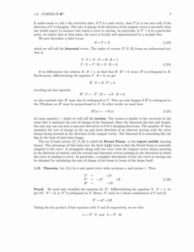
1.2. CURVES IN R3 7

It makes sense to call κ the curvature since, if T is a unit vector, then T ′(s) is not zero only if thedirection of T is changing. The rate of change of the direction of the tangent vector is precisely whatone would expect to measure how much a curve is curving. In particular, it T ′ = 0 at a particularpoint, we expect that at that point, the curve is locally well approximated by a straight line.

We now introduce a third vectorB = T ×N, (1.23)

which we will call the binormal vector. The triplet of vectors (T,N,B) forms an orthonormal set;that is,

T · T = N ·N = B ·B = 1T ·N = T ·B = N ·B = 0. (1.24)

If we differentiate the relation B · B = 1, we find that B · B′ = 0, hence B′ is orthogonal to B.Furthermore, differentiating the equation T ·B = 0, we get

B′ · T +B · T ′ = 0.

rewriting the last equationB′ · T = −T ′ ·B = −κN ·B = 0,

we also conclude that B′ must also be orthogonal to T . This can only happen if B′ is orthogonal tothe TB-plane, so B′ must be proportional to N . In other words, we must have

B′(s) = −τN(s) (1.25)

for some quantity τ , which we will call the torsion. The torsion is similar to the curvature in thesense that it measures the rate of change of the binormal. Since the binormal also has unit length,the only way one can have a non-zero derivative is if B is changing directions. The quantity B′ thenmeasures the rate of change in the up and down direction of an observer moving with the curvealways facing forward in the direction of the tangent vector. The binormal B is something like theflag in the back of sand dune buggy.

The set of basis vectors T,N,B is called the Frenet Frame or the repere mobile (movingframe). The advantage of this basis over the fixed (i,j,k) basis is that the Frenet frame is naturallyadapted to the curve. It propagates along with the curve with the tangent vector always pointingin the direction of motion, and the normal and binormal vectors pointing in the directions in whichthe curve is tending to curve. In particular, a complete description of how the curve is curving canbe obtained by calculating the rate of change of the frame in terms of the frame itself.

1.15 Theorem Let β(s) be a unit speed curve with curvature κ and torsion τ . Then

T ′ = κNN ′ = −κT τBB′ = −τB

. (1.26)

Proof: We need only establish the equation for N ′. Differentiating the equation N · N = 1, weget 2N ·N ′ = 0, so N ′ is orthogonal to N. Hence, N ′ must be a linear combination of T and B.

N ′ = aT + bB.

Taking the dot product of last equation with T and B respectively, we see that

a = N ′ · T, and b = N ′ ·B.


On the other hand, differentiating the equations N · T = 0, and N ·B = 0, we find that

N ′ · T = −N · T ′ = −N · (κN) = −κN ′ ·B = −N ·B′ = −N · (−τN) = τ.

We conclude that a = −κ, b = τ , and thus

N ′ = −κT + τB.

The Frenet frame equations (1.26) can also be written in matrix form as shown below. TNB

′ =

0 κ 0−κ 0 τ0 −τ 0

TNB

. (1.27)

The group-theoretic significance of this matrix formulation is quite important and we will comeback to this later when we talk about general orthonormal frames. At this time, perhaps it sufficesto point out that the appearance of an antisymmetric matrix in the Frenet equations is not at allcoincidental.

The following theorem provides a computational method to calculate the curvature and torsiondirectly from the equation of a given unit speed curve.

1.16 Proposition Let β(s) be a unit speed curve with curvature κ > 0 and torsion τ . Then

κ = ‖β′′(s)‖

τ =β′ · [β′′ × β′′′]

β′′ · β′′(1.28)

Proof: If β(s) is a unit speed curve, we have β′(s) = T . Then

T ′ = β′′(s) = κN,

β′′ · β′′ = (κN) · (κN),β′′ · β′′ = κ2

κ2 = ‖β′′‖2

β′′′(s) = κ′N + κN ′

= κ′N + κ(−κT + τB)= κ′N +−κ2T + κτB.

β′ · [β′′ × β′′′] = T · [κN × (κ′N +−κ2T + κτB)]= T · [κ3B + κ2τT ]= κ2τ

τ =β′ · [β′′ × β′′′]

κ2

=β′ · [β′′ × β′′′]

β′′ · β′′

1.17 Example Consider a circle of radius r whose equation is given by

α(t) = (r cos t, r sin t, 0).

1.2. CURVES IN R3 9

Then,

α′(t) = (−r sin t, r cos t, 0)

‖α′(t)‖ =√

(−r sin t)2 + (r cos t)2 + 02

=√r2(sin2 t+ cos2 t)

= r.

Therefore, ds/dt = r and s = rt, which we recognize as the formula for the length of an arc of circleof radius t, subtended by a central angle whose measure is t radians. We conclude that

β(s) = (−r sins

r, r cos

s

r, 0)

is a unit speed reparametrization. The curvature of the circle can now be easily computed

T = β′(s) = (− coss

r,− sin

s

r, 0)

T ′ = (1r

sins

r,−1

rcos

s

r, 0)

κ = ‖β′′‖ = ‖T ′‖

=

√1r2

sin2 s

r+

1r2

cos2s

r+ 02

=

√1r2

(sin2 s

r+ cos2

s

r)

=1r

This is a very simple but important example. The fact that for a circle of radius r the curvatureis κ = 1/r could not be more intuitive. A small circle has large curvature and a large circle has smallcurvature. As the radius of the circle approaches infinity, the circle locally looks more and more likea straight line, and the curvature approaches 0. If one were walking along a great circle on a verylarge sphere (like the earth) one would be perceive the space to be locally flat.

1.18 Proposition Let α(t) be a curve of velocity V, acceleration A, speed v and curvature κ,then

V = vT,

A =dv

dtT + v2κN. (1.29)

Proof: Let s(t) be the arclength and let β(s) be a unit speed reparametrization. Then α(t) =β(s(t)) and by the chain rule

V = α′(t)= β′(s(t))s′(t)= vT

A = α′′(t)

=dv

dtT + vT ′(s(t))s′(t)

=dv

dtT + v(κN)v

=dv

dtT + v2κN


Equation 1.29 is important in physics. The equation states that a particle moving along a curvein space feels a component of acceleration along the direction of motion whenever there is a changeof speed, and a centripetal acceleration in the direction of the normal whenever it changes direction.The centripetal acceleration and any point is

a = v3κ =v2

r

where r is the radius of a circle which has maximal tangential contact with the curve at the pointin question. This tangential circle is called the osculating circle. The osculating circle can beenvisioned by a limiting process similar to that of the tangent to a curve in differential calculus.Let p be point on the curve, and let q1 and q2 two nearby points. The three points determine acircle uniquely. This circle is a “secant” approximation to the tangent circle. As the points q1 andq2 approach the point p, the “secant” circle approaches the osculating circle. The osculating circlealways lies in the the TN -plane, which by analogy, is called the osculating plane.

1.19 Example (Helix)

β(s) = (a cosωs

c, a sin

ωs

c,bs

c), where c =

√a2ω2 + b2

β′(s) = (−aωc

sinωs

c,aω

ccos

ωs

c,b

c)

β′′(s) = (−aω2

c2cos

ω2s

c,−aω

2

c2sin

ωs

c, 0)

beta′′′(s) = (−aω3

c3cos

ω2s

c,−aω

3

c3sin

ωs

c, 0)

κ2 = β′′ · β′′

=a2ω4

c4

κ = ±aω2

c2

τ =(β′β′′β′′′)β′′ · β′′

=b

c

[−aω2

c2 cos ωsc −aω2

c2 sin ωsc

aω3

c2 sin ωsc −aω3

c2 cos ωsc

]c4

a2ω4.

=b

c

a2ω5

c5c4

a2ω4

Simplifying the last expression and substituting the value of c, we get

τ =bω

a2ω2 + b2

κ = ± aω2

a2ω2 + b2

Notice that if b = 0 the helix collapses to a circle in the xy-plane. In this case the formulas abovereduce to κ = 1/a and τ = 0. The ratio κ/τ = aω/b is particularly simple. Any curve whereκ/τ = constant is called a helix, of which the circular helix is a special case.

1.20 Example (Plane curves) Let α(t) = (x(t), y(t), 0). Then

α′ = (x′, y′, 0)

1.2. CURVES IN R3 11

α′′ = (x′′, y′′, 0)α′′′ = (x′′′, y′′′, 0)

κ =‖α′ × α′′‖‖α′‖3

=| x′y′′ − y′x′′ |(x′2 + y′2)3/2

τ = 0

1.21 Example (Cornu Spiral) Let β(s) = (x(s), y(s), 0), where

x(s) =∫ s

0

cost2

2c2dt

y(s) =∫ s

0

sint2

2c2dt. (1.30)

Then, using the fundamental theorem of calculus, we have

β′(s) = (coss2

2c2, sin

t2

2c2, 0),

Since ‖β′ = v = 1‖, the curve is of unit speed, and s is indeed the arc length. The curvature is ofthe Cornu spiral is given by

κ = | x′y′′ − y′x′′ |= (β′ · β′)1/2

= ‖ − s

c2sin

t2

2c2,s

c2cos

t2

2c2, 0‖

=s

c2.

The integrals (1.30) defining the coordinates of the Cornu spiral are the classical Frenel Integrals.These functions, as well as the spiral itself arise in the computation of the diffraction pattern of acoherent beam of light by a straight edge.

In cases where the given curve α(t) is not of unit speed, the following proposition providesformulas to compute the curvature and torsion in terms of α

1.22 Proposition If α(t) is a regular curve in R3 , then

κ2 =‖α′ × α′′‖2

‖α′‖6(1.31)

τ =(α′α′′α′′′)‖α′ × α′′‖2

, (1.32)

where (α′α′′α′′′) is the triple vector product [α×′ α′′] · α′′′.Proof:

α′ = vT

α′′ = v′T + v2κN

α′′′ = (v2κ)N ′((s(t))s′(t) + . . .

= v3κN ′ + . . .

= v3κτB + . . .


The other terms are unimportant here because as we will see α′ × α′′ is proportional to B

α′ × α′′ = v3κ(T ×N) = v3κB

‖α′ × α′′‖ = v3κ

κ =‖α′ × α′′‖

v3

(α′ × α′′) · α′′′ = v6κ2τ

τ =(α′α′′α′′′)v6κ2

=(α′α′′α′′′)‖α′ × α′′‖2

1.3 Fundamental Theorem of Curves

Some geometrical insight into the significance of the curvature and torsion can be gained by consid-ering the Taylor series expansion of an arbitrary unit speed curve β(s) about s = 0

β(s) = β(0) + β′(0)s+β′′(0)

2!s2 +

β′′′(0)3!

s3 + . . . (1.33)

Since we are assuming that s is an arclength parameter,

β′(0) = T (0) = T0

β′′(0) = (κN)(0) = κ0N0

β′′′(0) = (−κ2T + κ′N + κτB)(0) = −κ20T0 + κ′0N0 + κ0τ0B0

Keeping only the lowest terms in the components of T , N , and B, we get the first order Frenetapproximation to the curve

β(s) .= β(0) + T0s+12κ0N0s

2 +16κ0τ0B0s

3. (1.34)

The first two terms represent the linear approximation to the curve. The first three termsapproximate the curve by a parabola which lies in the osculating plane (TN -plane). If κ0 = 0, thenlocally the curve looks like a straight line. If τ0 = 0, then locally the curve is a plane curve whichlies on the osculating plane. In this sense, the curvature measures the deviation of the curve frombeing a straight line and the torsion (also called the second curvature) measures the deviation of thecurve from being a plane curve.

1.23 Theorem (Fundamental Theorem of Curves) Let κ(s) and τ(s), (s > 0) be any two analyticfunctions. Then there exists a unique curve (unique up to its position in R3 ) for which s is thearclength, κ(s) its curvature and τ(s) its torsion.Proof: Pick a point in R3 . By an appropriate affine transformation, we may assume that thispoint is the origin. Pick any orthogonal frame T,NB. The curve is then determined uniquely byits Taylor expansion in the Frenet frame as in equation (1.34).

1.24 Remark It is possible to prove the theorem just assuming that κ(s) and τ(s) are continuous.The proof however, becomes much harder and we refer the reader to other standard texts for theproof.

1.25 Proposition A curve with κ = 0 is part of a straight line.we leave the proof as an exercise.

1.3. FUNDAMENTAL THEOREM OF CURVES 13

1.26 Proposition A curve α(t) with τ = 0 is a plane curve.Proof: If τ = 0, then (α′α′′α′′′) = 0. This means that the three vectors α′, α′′, and α′′′ are linearlydependent and hence there exist functions a1(s),a2(s) and a3(s) such that

a3α′′′ + a2α

′′ + a1α′ = 0.

This linear homogeneous equation will have a solution of the form

α = c1α1 + c2α2 + c3, ci = constant vectors.

This curve lies in the plane

(x− c3) · n = 0, where n = c1 × c2

Chapter 2

Differential Forms

2.1 1-Forms

One of the most puzzling ideas in elementary calculus is the idea of the differential. In the usualdefinition, the differential of a dependent variable y = f(x), is given in terms of the differential ofthe independent variable by dy = f ′(x)dx. The problem is with the quantity dx. What does dxmean? What is the difference between ∆x and dx? How much ”smaller” than ∆x does dx haveto be? There is no trivial resolution to this question. Most introductory calculus texts evade theissue by treating dx as an arbitrarily small quantity (which lacks mathematical rigor) or by simplyreferring to dx as an infinitesimal (a term introduced by Newton for an idea that could not otherwisebe clearly defined at the time.)

In this section we introduce linear algebraic tools that will allow us to interpret the differentialin terms of an linear operator.

2.1 Definition Let p ∈ Rn, and let Tp(Rn) be the tangent space at p. A 1-form at p is a linearmap φ from Tp(Rn) into R. We recall that such a map must satisfy the following properties

a) φ(Xp) ∈ R, ∀Xp ∈ Rn (2.1)b) φ(aXp + bYp) = aφ(Xp) + bφ(Yp), ∀a, b ∈ R, Xp, Yp ∈ Tp(Rn)

A 1-form is a smooth choice of a linear map φ as above for each point in the space.

2.2 Definition Let f : Rn → R be a real-valued C∞ function. We define the differential df ofthe function as the 1-form such that

df(X) = X(f) (2.2)

for every vector field in X in Rn.In other words, at any point p, the differential df of a function is an operator which assigns to

a tangent vector Xp, the directional derivative of the function in the direction of that vector

df(X)(p) = Xp(f) = ∇f(p) ·X(p) (2.3)

In particular, if we apply the differential of the coordinate functions xi to the basis vector fields,we get

dxi(∂

∂xj) =

∂xi

∂xj= δi

j (2.4)

The set of all linear functionals on a vector space is called the dual of the vector space. It isan standard theorem in linear algebra that the dual of a vector space is also a vector space of the

15

16 CHAPTER 2. DIFFERENTIAL FORMS

same dimension. Thus, the space T ?p Rn of all 1-forms at p is a vector space which is the dual of

the tangent space TpRn. The space T ?p (Rn) is called the cotangent space of Rn at the point p.

Equation (2.4) indicates that the set of differential forms (dx1)p, . . . , (dxn)p constitutes the basisof the cotangent space which is dual to the standard basis ( ∂

∂x1 )p, . . . ( ∂∂xn )p of the tangent space.

The union of all the cotangent spaces as p ranges over all points in Rn is called the cotangent bundleT ∗(Rn).

2.3 Proposition Let f be any smooth function in Rn and let x1, . . . xn be coordinate functionsin a neighborhood U of a point p. Then, the differential df is given locally by the expression

df =n∑

i=1

∂f

∂xidxi (2.5)

=∂f

∂xidxi

Proof: The differential df is by definition a 1-form, so, at each point, it must be expressible as alinear combination of the basis elements (dx1)p, . . . , (dxn)p. Therefore, to prove the proposition,it suffices to show that the expression 2.5 applied to an arbitrary tangent vector, coincides withdefinition 2.2. To see this, consider a tangent vector Xp = aj( ∂

∂xj )p and apply the expression above

(∂f

∂xidxi)p(Xp) = (

∂f

∂xidxi)(aj ∂

∂xj)(p) (2.6)

= aj(∂f

∂xidxi)(

∂

∂xj)(p)

= aj(∂f

∂xi

∂xi

∂xj)(p)

= aj(∂f

∂xiδij)(p)

= (∂f

∂xiai)(p)

= ∇f(p) ·X(p)= df(X)(p)

The definition of differentials as linear functionals on the space of vector fields is much moresatisfactory than the notion of infinitesimals, since the new definition is based on the rigorousmachinery of linear algebra. If α is an arbitrary 1-form, then locally

α = a1(x)dx1+, . . .+ an(x)dxn, (2.7)

where the coefficients ai are C∞ functions. A 1-form is also called a covariant tensor of rank 1,or just simply a covector. The coefficients (a1, . . . , an) are called the covariant components ofthe covector. We will adopt the convention to always write the covariant components of a covectorwith the indices down. Physicists often refer to the covariant components of a 1-form as a covariantvector and this causes some confusion about the position of the indices. We emphasize that not allone forms are obtained by taking the differential of a function. If there exists a function f , suchthat α = df , then the one form α is called exact. In vector calculus and elementary physics, exactforms are important in understanding the path independence of line integrals of conservative vectorfields.

As we have already noted, the cotangent space T ∗p (Rn) of 1-forms at a point p has a naturalvector space structure. We can easily extend the operations of addition and scalar multiplication to

2.2. TENSORS AND FORMS OF HIGHER RANK 17

the space of all 1-forms by defining

(α+ β)(X) = α(X) + β(X) (2.8)(fα)(X) = fα(X)

for all vector fields X and all smooth functions f .

2.2 Tensors and Forms of Higher Rank

As we mentioned at the beginning of this chapter, the notion of the differential dx is not madeprecise in elementary treatments of calculus, so consequently, the differential of area dxdy in R2, aswell as the differential of surface area in R3 also need to be revisited in a more rigorous setting. Forthis purpose, we introduce a new type of multiplication between forms which not only captures theessence of differentials of area and volume, but also provides a rich algebraic and geometric structurewhich is vast generalization of cross products (which only make sense in R3) to Euclidean spaces ofall dimensions.

2.4 Definition A map φ : T (Rn)× T (Rn) −→ R is called a bilinear map on the tangent space,if it is linear on each slot. That is

φ(f1X1 + f2X2, Y1) = f1φ(X1, Y1) + f2φ(X2, Y1)φ(X1, f

1Y1 + f2Y2) = f1φ(X1, Y1) + f2φ(X1, Y2), ∀Xi, Yi ∈ T (Rn), f i ∈ C∞Rn

Tensor Products

2.5 Definition Let α and β be 1-forms. The tensor product of α and β is defined as the bilinearmap α⊗ β such that

(α⊗ β)(X,Y ) = α(X)β(Y ) (2.9)

for all vector fields X and Y .Thus, for example, if α = aidx

i and β = bjdxj , then,

(α⊗ β)(∂

∂xk,∂

∂xl) = α(

∂

∂xk)β(

∂

∂xl)

= (aidxi)(

∂

∂xk)(bjdxj)(

∂

∂xl)

= aiδikbjδ

jl

= akbl

A quantity of the form T = Tijdxi⊗dxj is called a covariant tensor of rank 2, and we may think

of the set dxi⊗ dxj as a basis for all such tensors. We must caution the reader again that there ispossible confusion about the location of the indices, since physicists often refer to the componentsTij as a covariant tensor.

In a similar fashion, one can also define the tensor product of vectors X and Y as the bilinearmap X ⊗ Y such that

(X ⊗ Y )(f, g) = X(f)Y (g) (2.10)

for any pair of arbitrary functions f and g.


If X = ai ∂∂xi and Y = bj ∂

∂xj , then, the components of X ⊗ Y in the basis ∂∂xi ⊗ ∂

∂xj are simplygiven by aibj . Any bilinear map of the form

T = T ij ∂

∂xi⊗ ∂

∂xj(2.11)

is called a contravariant tensor of rank 2 in Rn .The notion of tensor products can easily be generalized to higher rank, and in fact one can have

tensors of mixed ranks. For example, a tensor of contravariant rank 2 and covariant rank 1 in Rn isrepresented in local coordinates by an expression of the form

T = T ijk

∂

∂xi⊗ ∂

∂xj⊗ dxk.

This object is also called a tensor of type T 2,1. Thus, we may think of a tensor of type T 2,1 as mapwith three input slots. The map expects two functions in the first two slots and a vector in the thirdone. The action of the map is bilinear on the two functions and linear on the vector. The output isa real number. An assignment of a tensor to each point in Rn is called a tensor field.

Inner Products

Let X = ai ∂∂xi and Y = bj ∂

∂xj be two vector fields and let

g(X,Y ) = δijaibj . (2.12)

The quantity g(X,Y ) is an example of a bilinear map which the reader will recognize as the usualdot product.

2.6 Definition A bilinear map g(X,Y ) on the tangent space is called a vector inner product if

1. g(X,Y ) = g(Y,X),

2. g(X,X) ≥ 0, ∀X,

3. g(X,X) = 0 iff X = 0.

Since we assume g(X,Y ) to be bilinear, an inner product is completely specified by its action onordered pairs of basis vectors. The components gij of the inner product as thus given by

g(∂

∂xi,∂

∂xj) = gij (2.13)

where gij is a symmetric n× n matrix, which we assume to be non-singular. By linearity, it is easyto see that if X = ai ∂

∂xi and Y = bj ∂∂xj are two arbitrary vectors, then

g(X,Y ) = gijaibj .

In this sense, an inner product can be viewed as a generalization of the dot product. The standardEuclidean inner product is obtained if we take gij = δij . In this case the quantity g(X,X) =‖ X ‖2gives the square of the length of the vector. For this reason gij is also called a metric and g is calleda metric tensor.

Another interpretation of the dot product can be seen if instead one considers a vector X = ai ∂∂xi

and a 1-form α = bjdxj . The action of the 1-form on the vector gives

α(X) = (bjdxj)(ai ∂

∂xi)

= bjai(dxj)(

∂

∂xi)

= bjaiδj

i

= aibi.


If we now definebi = gijb

j , (2.14)we see that the equation above can be rewritten as

aibj = gijaibj ,

and we recover the expression for the inner product.Equation (2.14) shows that the metric can be used as mechanism to lower indices, thus trans-

forming the contravariant components of a vector to covariant ones. If we let gij be the inverse ofthe matrix gij , that is

gikgkj = δij , (2.15)

we can also raise covariant indices by the equation

bi = gijbj (2.16)We have mentioned that the tangent and cotangent spaces of Euclidean space at a particular point

are isomorphic. In view of the above discussion, we see that the metric accepts a dual interpretation;one as bilinear pairing of two vectors

g : T (Rn)× T (Rn) −→ R

and another as a linear isomorphism

g : T ?(Rn) −→ T (Rn)

that maps vectors to covectors and vice-versa.In elementary treatments of calculus authors often ignore the subtleties of differential 1-forms

and tensor products and define the differential of arclength as

ds2 ≡ gijdxidxj ,

although, what is really meant by such an expression is

ds2 ≡ gijdxi ⊗ dxj . (2.17)

2.7 Example In cylindrical coordinates, the differential of arclength is

ds2 = dr2 + r2dθ2 + dz2. (2.18)

In this case the metric tensor has components

gij =

1 0 00 r2 00 0 1

. (2.19)

2.8 Example In spherical coordinates

x = ρ sin θ cosφy = ρ sin θ sinφz = ρ cos θ, (2.20)

the differential of arclength is given by

ds2 = dρ2 + ρ2dθ2 + ρ2 sin2 θdφ2. (2.21)

In this case the metric tensor has components

gij =

1 0 00 ρ2 00 0 ρ2 sin θ2

. (2.22)


Minkowski Space

An important object in mathematical physics is the so called Minkowski space which is can bedefined as the pair Let (M1,3, g) be the pair, where

M(1,3) = (t, x1, x2, x3)| t, xi ∈ R (2.23)

and g is the bilinear map such that

g(X,X) = −t2 + (x1)2 + (x2)2 + (x3)2. (2.24)

The matrix representing Minkowski’s metric g is given by

g = diag(−1, 1, 1, 1),

in which case, the differential of arclength is given by

ds2 = gµνdxµ ⊗ dxν

= −dt⊗ dt+ dx1 ⊗ dx1 + dx2 ⊗ dx2 + dx3 ⊗ dx3

= −dt2 + (dx1)2 + (dx2)2 + (dx3)2. (2.25)

Note: Technically speaking, Minkowski’s metric is not really a metric since g(X,X) = 0 doesnot imply that X = 0. Non-zero vectors with zero length are called Light-like vectors and they areassociated with with particles which travel at the speed of light (which we have set equal to 1 in oursystem of units.)

The Minkowski metric gµν and its matrix inverse gµν are also used to raise and lower indices inthe space in a manner completely analogous to Rn . Thus, for example, if A is a covariant vectorwith components

Aµ = (ρ,A1, A2, A3),

then the contravariant components of A are

Aµ = gµνAν

= (−ρ,A1, A2, A3)

Wedge Products and n-Forms

2.9 Definition A map φ : T (Rn)× T (Rn) −→ R is called alternating if

φ(X,Y ) = −φ(Y,X)

The alternating property is reminiscent of determinants of square matrices which change sign ifany two column vectors are switched. In fact, the determinant function is a perfect example of analternating bilinear map on the space M2×2 of two by two matrices. Of course, for the definitionabove to apply, one has to view M2×2 as the space of column vectors.

2.10 Definition A 2-form φ is a map φ : T (Rn) × T (Rn) −→ R which is alternating andbilinear.

2.11 Definition Let α and β be 1-forms in Rn and let X and Y be any two vector fields. Thewedge product of the two 1-forms is the map α∧β : T (Rn)×T (Rn) −→ R given by the equation

(α ∧ β)(X,Y ) = α(X)β(Y )− α(Y )β(X) (2.26)


2.12 Theorem If α and β are 1-forms, then α ∧ β is a 2-form.Proof: : We break up the proof into the following two lemmas.

2.13 Lemma The wedge product of two 1-forms is alternating.Proof: Let α and β be 1-forms in Rn and let X and Y be any two vector fields. then

(α ∧ β)(X,Y ) = α(X)β(Y )− α(Y )β(X)= −(α(Y )β(X)− α(X)β(Y ))= −(α ∧ β)(Y,X)

2.14 Lemma The wedge product of two 1-forms is bilinear.Proof: Consider 1-forms, α, β, vector fields X1, X2, Y and functions f1, F 2. Then, since the1-forms are linear functionals, we get

(α ∧ β)(f1X1 + f2X2, Y ) = α(f1X1 + f2X2)β(Y )− α(Y )β(f1X1 + f2X2)= [f1α(X1) + f2α(X2)]β(Y )− α(Y )[f1β(X1) + f2α(X2)]= f1α(X1)β(Y ) + f2α(X2)β(Y ) + f1α(Y )β(X1) + f2α(Y )β(X2)= f1[α(X1)β(Y ) + α(Y )β(X1)] + f2[α(X2)β(Y ) + α(Y )β(X2)]= f1(α ∧ β)(X1, Y ) + f2(α ∧ β)(X2, Y )

The proof of linearity on the second slot is quite similar and it is left to the reader.

2.15 Corollary If α and β are 1-forms, then

α ∧ β = −β ∧ α (2.27)

This last result tells us that wedge products have characteristics similar to cross products ofvectors in the sense that both of these products are anti-commutative. This means that we need tobe careful to introduce a minus sign every time we interchange the order of the operation. Thus, forexample, we have

dxi ∧ dxj = −dxj ∧ dxi

if i 6= j, whereasdxi ∧ dxi = −dxi ∧ dxi = 0

since any quantity which is equal to the negative of itself must vanish. The similarity between wedgeproducts is even more striking in the next proposition but we emphasize again that wedge productsare by far much more powerful than cross products, because wedge products can be computed inany dimension.

2.16 Proposition Let α = Aidxi and β = Bidx

i be any two 1-forms in Rn . Then

α ∧ β = (AiBj)dxi ∧ dxj (2.28)

Proof: Let X and Y be arbitrary vector fields. Then

(α ∧ β)((X,Y ) = (Aidxi)(X)(Bjdx

j)(Y )− (Aidxi)(Y )(Bjdx

j)(X)= (AiBj)[dxi(X)dxj(Y )− dxi(Y )dxj(X)]= (AiBj)(dxi ∧ dxj)(X,Y )


Because of the antisymmetry of the wedge product the last equation above can also be written as

α ∧ β =n∑

i=1

n∑j<i

(AiBj −AjBi)(dxi ∧ dxj)

In particular, if n = 3, then the coefficients of the wedge product are the components of the crossproduct of A = A1i +A2j +A3k and B = B1i +B2j +B3k

2.17 Example Let α = x2dx− y2dy and β = dx+ dy − 2xydz. Then

α ∧ β = (x2dx− y2dy) ∧ (dx+ dy − 2xydz)= x2dx ∧ dx+ x2dx ∧ dy − 2x3ydx ∧ dz − y2dy ∧ dx− y2dy ∧ dy + 2xy3dy ∧ dz= x2dx ∧ dy − 2x3ydx ∧ dz − y2dy ∧ dx+ 2xy3dy ∧ dz= (x2 + y2)dx ∧ dy − 2x3ydx ∧ dx+ 2xy3dy ∧ dz

2.18 Example let x = r cos θ and y = r sin θ. Then

dx ∧ dy = (−r sin θdθ + cos θdr) ∧ (r cos θdθ + sin θdr)= −r sin2 θdθ ∧ dr + r cos2 θdr ∧ dθ= (r cos2 θ + r sin2 θ)(dr ∧ dθ)= r(dr ∧ dθ) (2.29)

2.19 Remark

1. The result of the last example yields the familiar differential of area in polar coordinates

2. The differential of area in polar coordinates is a special example of the change of coordinatetheorem for multiple integrals. It is easy to establish that if x = f1(u, v) and y = f2(u, v), thendx∧dy = det|J |du∧dv, where det|J | is the determinant of the Jacobian of the transformation.

3. Quantities such as dxdy and dydz which often appear in calculus, are not well defined. Inmost cases what is meant by these entities are wedge products of 1-forms

4. We state (without proof) that all 2-forms φ in Rn can be expressed as linear combinations ofwedge products of differentials such as

φ = Fijdxi ∧ dxj (2.30)

In a more elementary (ie: sloppier) treatment of this subject one could simply define 2-formsto be gadgets which look like the quantity in equation (2.30). This is fact what we will do inthe next definition.

2.20 Definition A 3=form φ in Rn is an object of the following type

φ = Aijkdxi ∧ dxj ∧ dxk (2.31)

where we assume that the wedge product of three 1-forms is associative, but still alternating inthe sense that if one switches any two differentials, then the entire expression changes by a minussign. we challenge the reader to come up with a rigorous definition of three forms (or an n-form,for that matter) more in the spirit of multilinear maps. There is nothing really wrong with using

2.3. EXTERIOR DERIVATIVES 23

definition ref3form. It is just that this definition is coordinate dependent and mathematicians ingeneral (specially differential geometers) prefer coordinate-free definitions, theorems and proofs.

And now, a little combinatorics. Let us count the number of differential forms in Euclideanspace. More specifically, we want to count the dimensions of the space of k-forms in Rn in thesense of vector spaces. We will thing of 0-forms as being ordinary functions. Since functions are the”scalars”, the space of 0-forms as a vector space has dimension 1.

R2 Forms Dim0-forms f 11-forms fdx1, gdx2 22-forms fdx1 ∧ dx2 1

R3 Forms Dim0-forms f 11-forms f1dx

1, f2dx2, f3dx

3 32-forms f1dx

2 ∧ dx3, f2dx3 ∧ dx1, f3dx1 ∧ dx2 33-forms f1dx

1 ∧ dx2 ∧ dx3 1

The binomial coefficient pattern should be evident to the reader.

2.3 Exterior Derivatives

In this section we introduce a differential operator which generalizes the classical gradient, curl anddivergence operators.

Denote by∧m

(p)(Rn) the space of m-forms at p ∈ Rn. This vector space has dimension

dim∧m

(p)(Rn) =

n!m!(n−m)!

for m ≤ n and dimension 0 if m > n. We shall identify∧0

(p)(Rn) with the space of C∞ functions at

p. Also we will call∧m(Rn) the union of all

∧m(p)(R

n) as p ranges through all the points in Rn .In other words, we have ∧m(Rn) =

⋃p

∧mp (Rn).

If α ∈∧m(Rn), then α can be written in the form

α = Ai1,...im(x)dxi1 ∧ . . . dxim (2.32)

.

2.21 Definition Let α be an m-form (written in coordinates as in equation (2.32)). The exteriorderivative of α is the (m+1-form) dα given by

dα = dAi1,...im ∧ dxi0 ∧ dxi1 . . . dxim

=∂Ai1,...im

∂dxi0(x)dxi0 ∧ dxi1 . . . dxim (2.33)

In the special case where α is a 0-form, that is, a function, we write

df =∂f

∂xidxi


2.22 Proposition

a) d :∧m −→

∧m+1

b) d2 = d d = 0c) d(α ∧ β) = dα ∧ β + (−1)pα ∧ dβ ∀α ∈

∧p, β ∈

∧q (2.34)

Proof:a) Obvious from equation (2.32).b) First we prove the proposition for α = f ∈

∧0. We have

d(dα) = d(∂f

∂dxi)

=∂2f

∂xj∂xidxj ∧ dxi

=12[∂2f

∂xj∂xi

∂2f

∂xi∂xj]dxj ∧ dxi

= 0

Now, suppose that α is represented locally as in equation (2.32). It follows from 2.33 that

d(dα) = d(dAi1,...im) ∧ dxi0 ∧ dxi1 . . . dxim = 0

c) Let α ∈∧p, β ∈

∧q. Then we can write

α = Ai1,...ip(x)dxi1 ∧ . . . dxip

β = Bj1,...jq(x)dxj1 ∧ . . . dxjq .

(2.35)

By definition,α ∧ β = Ai1...ip

Bj1...jq(dxi1 ∧ . . . ∧ dxip) ∧ (dxj1 ∧ . . . ∧ dxjq )

Now we take take the exterior derivative of the last equation taking into account that d(fg) =fdg + gdf for any functions f and g. We get

d(α ∧ β) = [d(Ai1...ip)Bj1...jq

+ (Ai1...ipd(Bj1...jq

)](dxi1 ∧ . . . ∧ dxip) ∧ (dxj1 ∧ . . . ∧ dxjq )

= [dAi1...ip∧ (dxi1 ∧ . . . ∧ dxip)] ∧ [Bj1...jq

∧ (dxj1 ∧ . . . ∧ dxjq )] +

= [Ai1...ip ∧ (dxi1 ∧ . . . ∧ dxip)] ∧ (−1)p[dBj1...jq ∧ (dxj1 ∧ . . . ∧ dxjq )]= dα ∧ β + (−1)pα ∧ dβ. (2.36)

The (−1)p factor comes in because to pass the term dBji...jp through p 1-forms of the type dxi, onehas to perform p transpositions.

2.23 Example Let α = P (x, y)dx+Q(x, y)dβ. Then,

dα = (∂P

∂xdx+

∂P

∂y) ∧ dx+ (

∂Q

∂xdx+

∂Q

∂y) ∧ dy

=∂P

∂ydy ∧ dx+

∂Q

∂xdx ∧ dy

= (∂Q

∂x− ∂P

∂y)dx ∧ dy. (2.37)

This example is related to Green’s theorem in R2.

2.4. THE HODGE-∗ OPERATOR 25

2.24 Example Let α = M(x, y)dx+N(x, y)dy, and suppose that dα = 0. Then, by the previousexample,

dα = (∂N

∂x− ∂M

∂y)dx ∧ dy.

Thus, dα = 0 iff Nx = My which implies that N = fy and Mx for some C1 function f(x, y). Hence

α = fxdx+ fydf = df.

The reader should also be familiar with this example in the context of exact differential equationsof first order, and conservative force fields.

2.25 Definition A differential form α is called closed if dα = 0.

2.26 Definition A differential form α is called exact if there exist a form β such that α = dβ.Since d d = 0, it is clear that a exact form is also closed. The converse is not at all obvious ingeneral and we state it here without proof.

2.27 Poincare’s Lemma In a simply connected space (such as Rn ), if a differential is closedthen it is exact.The assumption hypothesis that the space must be simply connected is somewhat subtle. Thecondition is reminiscent of Cauchy’s integral theorem for functions of a complex variable, whichstates that if f(z) is holomorphic function and C is a simple closed curve, then,∮

C

f(z)dz = 0

This theorem does not hold if the region bounded by the curve C is not simply connected. Thestandard example is the integral of the complex 1-form ω = (1/z)dz around the unit circle Cbounding a punctured disk. In this case, ∮

C

1zdz = 2πi

2.4 The Hodge-∗ Operator

One of the important lessons that students learn in linear algebra is that all vector space of finitedimension n are isomorphic to each other. Thus, for instance, the space P3 of all real polynomialsin x of degree 3, and the space M2×2 of real 2 by 2 matrices, are basically no different than theEuclidean vector space R4 in terms of their vector space properties. We have already encountereda number of vector spaces of finite dimension in these notes. A good example of this is the tangentspace TpR3. The ”vector” part a1 ∂

∂x + a2 ∂∂y + a3 ∂

∂z can be mapped to a regular advanced calculusvector a1i + a2j + a3k, by replacing ∂

∂x by i, ∂∂y by j and ∂

∂z by k. Of course, we must not confusea tangent vector which is a linear operator with a Euclidean vector which is just an ordered triplet,but as far their vector space properties, there is basically no difference.

We have also observed that the tangent space TpRn is isomorphic to the cotangent space T ?p Rn .

In this case, the vector space isomorphism maps the standard basis vectors ∂∂xi to their duals

dxi. This isomorphism then transforms a contravariant vector to a covariant vector.Another interesting example is provided by the spaces

∧1p(R

3) and∧2

p(R3), both of which have

dimension 3. It follows that these two spaces must be isomorphic. In this case the isomorphism isgiven by the map

dx 7−→ dy ∧ dz


dy 7−→ −dx ∧ dzdz 7−→ dx ∧ dy

(2.38)

More generally, we have seen that the dimension of the space of m-forms in Rn is given by thebinomial coefficient (

nm). Since (n

m)

=(

nn−m

)=

n!(n−m)!

,

it must be the case that ∧mp (Rn) ∼=

∧mp (Rn−m) (2.39)

To describe the isomorphism between these two spaces, we will first need to introduce the totallyantisymmetric Levi-Civita permutation symbol which is defined as follows

εi1...im=

+1 if(i1, . . . , im) is an even permutation of(1, . . . ,m)−1 if(i1, . . . , im) is an odd permutation of(1, . . . ,m)0 otherwise

(2.40)

In dimension 3, there are only 3 (3!=6) nonvanishing components of εi,j,k in

ε123 = ε231 = ε312 = 1ε132 = ε213 = ε321 = 1 (2.41)

The permutation symbols are useful in the theory of determinants. In fact, if A = (aij) is a 3× 3

matrix, then, using equation (2.41), the reader can easily verify that

detA = |A| = εi1i2i3ai11 a

i22 a

i33 (2.42)

This formula for determinants extends in an obvious manner to n × n matrices. A more thoroughdiscussion of the Levi-Civita symbols will appear later in these notes.

In Rn , the Levi-Civita symbol with some or all the indices up is numerically equal to thepermutation symbol will all indices down

εi1...im = εi1...im ,

since the Euclidean metric used to raise and lower indices is δij .On the other hand, in Minkowski space, raising an index with a value of 0 costs a minus sign,

because g00 = g00 = −1. Thus, in calM(1,3)

εi0i1i2i3 = −εi0i1i2i3 ,

since any permutation of 0, 1, 2, 3 must contain a 0.

2.28 Definition The Hodge-∗ operator is a linear map ∗ :∧m

p (Rn) −→∧m

p (Rn−m) defined instandard local coordinates by the equation

∗(dxi1 ∧ . . . ∧ dxim) =1

(n−m)!εi1...im

im+1...indxim+1 ∧ . . . ∧ dxin , (2.43)

Since the forms dxi1∧. . .∧dxim constitute a basis of the vector space∧m

p (Rn) and the ∗-operatoris assumed to be a linear map, equation (2.43) completely specifies the map for all m-forms.


2.29 Example Consider the dimension n=3 case. then

∗dx1 =12!ε1 jkdx

j ∧ dxk

=12!

[ε1 23dx2 ∧ dx3 + ε1 32dx

3 ∧ dx2]

=12!

[dx2 ∧ dx3 − dx3 ∧ dx2]

=12!

[dx2 ∧ dx3 + dx2 ∧ dx3]

= dx2 ∧ dx3.

We leave it to reader to complete the computation of the action of the ∗-operator on the other basisforms. The results are

∗dx1 = +dx2 ∧ dx3

∗dx2 = −dx1 ∧ dx3

∗dx3 = +dx1 ∧ dx2, (2.44)

∗(dx2 ∧ dx3) = dx1

∗(−dx3 ∧ dx1) = dx2

∗(dx1 ∧ dx2) = dx3, (2.45)

and∗(dx1 ∧ dx2 ∧ dx3) = 1. (2.46)

In particular, if f : R3 −→ R is any 0-form (a function) then,

∗f = f(dx1 ∧ dx2 ∧ dx3)= fdV, (2.47)

where dV is the differential of volume, also called the volume form.

2.30 Example Let α = A1dx1A2dx

2 +A3dx3, and β = B1dx

1B2dx2 +B3dx

3. Then,

∗(α ∧ β) = (A2B3 −A3B2) ∗ (dx2 ∧ dx3) + (A1B3 −A3B1) ∗ (dx1 ∧ dx3) +(A1B2 −A2B1) ∗ (dx1 ∧ dx2)

= (A2B3 −A3B2)dx1 + (A1B3 −A3B1)dx2 + (A1B2 −A2B1)dx3

= (~A× ~B)idxi (2.48)

The previous examples provide some insight on the action of the ∧ and ∗ operators. If one thinksof the quantities dx1, dx2 and dx3 as playing the role of ~i, ~j and ~k, then it should be apparent thatequations 2.44 are the differential geometry versions of the well known relations

i = j× k

j = −i× k

k = i× j

. This is even more evident upon inspection of equation (2.48), which relates the ∧ operator to theCartesian cross product.


2.31 Example In Minkowski space the collection of all 2-forms has dimension (42) = 6. The Hodge-

∗ operator in this case, splits∧2(M1,3) into two 3-dim subspaces

∧2±, such that ∗ :

∧2± −→

∧2∓ .

More specifically,∧2

+ is spanned by the forms dx0 ∧ dx1, dx0 ∧ dx2, dx0 ∧ dx3, and∧2− is spanned

by the forms dx2 ∧ dx3,−dx1 ∧ dx3, dx1 ∧ dx2. The action of ∗ on∧2

+ is

∗(dx0 ∧ dx1) = 12ε

01kldx

k ∧ dxl = −dx2 ∧ dx3

∗(dx0 ∧ dx2) = 12ε

02kldx

k ∧ dxl = +dx1 ∧ dx3

∗(dx0 ∧ dx3) = 12ε

03kldx

k ∧ dxl = −dx1 ∧ dx2,

and on∧2−,

∗(+dx2 ∧ dx3) = 12ε

23kldx

k ∧ dxl = dx0 ∧ dx1

∗(−dx1 ∧ dx3) = 12ε

13kldx

k ∧ dxl = dx0 ∧ dx2

∗(+dx1 ∧ dx2) = 12ε

12kldx

k ∧ dxl = dx0 ∧ dx3,

In verifying the equations above, we recall that the Levi-Civita symbols which contain an indexwith value 0 in the up position have an extra minus sign as a result of raising the index with g00.IfF ∈

∧2(M), we will formally write F = F+ + F−, where F± ∈∧2±. We would like to note that the

action of the dual operator on∧2(M) is such that ∗

∧2(M) −→∧2(M), and ∗2 = −1. Thus, the

operator is an linear involution of the space and in fact,∧2± are the eigenspaces corresponding to

the two eigenvalues of this involution.It is also worthwhile to calculate the duals of 1-forms in M1,3. The results are

∗dt = −dx1 ∧ dx2 ∧ dx3

∗dx1 = +dx2 ∧ dt ∧ dx3

∗dx2 = +dt ∧ dx1 ∧ dx3

∗dx3 = +dx1 ∧ dt ∧ dx2. (2.49)

Gradient, Curl and Divergence

Classical differential operators which enter in Green’s and Stokes Theorems are better understood asspecial manifestations of the exterior differential and the Hodge-∗ operators in R3. Here is preciselyhow this works:

1. Let f : R3 −→ R be a C∞ function. Then

df =∂f

∂xjdxj = ∇f · dx (2.50)

2. Let α = Aidxi be a 1-form in R3. Then

(∗d)α =12(∂Ai

∂xj− ∂Ai

∂xj) ∗ (dxi ∧ dxj)

= (∇×A) · dx (2.51)

3. Let α = B1dx2 ∧ dx3 +B2dx

3 ∧ dx1 +B3dx1 ∧ dx2 be a 2-form in R3. Then

dα = (∂B1

∂x1+∂B2

∂x2+∂B3

∂x3)dx1 ∧ dx2 ∧ dx3

= (∇ ·B)dV (2.52)


4. Let α = Bidxi, then

∗d ∗ α = ∇ ·B (2.53)

It is also possible to define and manipulate formulas of classical vector calculus using the per-mutation symbols. For example, let a = (A1, A2, A3) and B = (B1, B2, B3) be any two Euclideanvectors. Then it is easy to see that

(A×B)k = εijkAiBj ,

and(∇×B)k = εijk

∂Ai

∂xj,

To derive many classical vector identities in this formalism, it is necessary to first establish thefollowing identity (see Ex. ())

εijmεklm = δikδ

jl − δi

lδjk (2.54)

2.32 Example

[A× (B×C)]l = εmnl A m(B×C)m

= εmnl Am(εjk

nBjCk)= εmn

l εjknAmBjCk)

= εmnlεjknAmBjCk)

= (δjl δ

km − δk

l δjn)AmBjCk

= BlAmCm − ClA

mbn

Or, rewriting in vector form

A× (B×C) = B(A ·C)−C(A ·B) (2.55)

Maxwell Equations

The classical equations of Maxwell describing electromagnetic phenomena are

∇ ·E = 4πρ ∇×B = 4πJ + ∂E∂t

∇ ·B = 0 ∇×E = −∂B∂t (2.56)

We would like to formulate these equations in the language of differential forms. Let xµ =(t, x1, x2, x3) be local coordinates in Minkowski’s space M1,3. Define the Maxwell 2-form F by theequation

F =12Fµνdx

µ ∧ dxν , (µ, ν = 0, 1, 2, 3), (2.57)

where

Fµν =

0 −Ex −Ey −Ey

Ex 0 Bz −By

Ey −Bz 0 Bx

Ez By −Bx 0

. (2.58)

Written in complete detail, Maxwell’s 2-form is given by

F = −Exdt ∧ dx1 − Eydt ∧ dx2 − Ezdt ∧ dx3 +Bzdx

1 ∧ dx2 −Bydx1 ∧ dx3 +Bxdx

2 ∧ dx3. (2.59)


We also define the source current 1-form

J = Jµdxµ = ρdt+ J1dx

1 + J2dx2 + J3dx

3. (2.60)

2.33 Proposition Maxwell’s Equations 2.56 are equivalent to the equations

dF = 0,d ∗ F = 4π ∗ J. (2.61)

Proof: The proof is by direct computation using the definitions of the exterior derivative andthe Hodge-∗ operator.

dF = −∂Ex

∂x2∧ dx2 ∧ dt ∧ dx1 − ∂Ex

∂x3∧ dx3 ∧ dt ∧ dx1 +

−∂Ey

∂x1∧ dx1 ∧ dt ∧ dx2 − ∂Ey

∂x3∧ dx3 ∧ dt ∧ dx2 +

−∂Ez

∂x1∧ dx1 ∧ dt ∧ dx3 − ∂Ez

∂x2∧ dx2 ∧ dt ∧ dx3 +

∂Bz

∂t∧ dt ∧ dx1 ∧ dx2 − ∂Bz

∂x3∧ dx3 ∧ dx1 ∧ dx2 −

∂By

∂t∧ dt ∧ dx1 ∧ dx3 − ∂By

∂x2∧ dx2 ∧ dx1 ∧ dx3 +

∂Bx

∂t∧ dt ∧ dx2 ∧ dx3 +

∂Bx

∂x1∧ dx1 ∧ dx2 ∧ dx3.

Collecting terms and using the antisymmetry of the wedge operator, we get,

dF = (∂Bx

∂x1+∂By

∂x2+∂Bz

∂x3)dx1 ∧ dx2 ∧ dx3 +

(∂Ey

∂x3− ∂Ez

∂x2− ∂Bx

∂t)dx2 ∧ dt ∧ dx3 +

(∂Ez

∂x1− ∂Ex

∂dx3− ∂By

∂t)dt ∧ dx1 ∧ x3 +

(∂Ex

∂x2− ∂Ey

∂x1− ∂Bz

∂t)dx1 ∧ dt ∧ dx2.

Therefore, dF = 0 iff∂Bx

∂x1+∂By

∂x2+∂By

∂x3= 0,

which is the same as∇ ·B = 0,

and

∂Ey

∂x3− ∂Ez

∂x2− ∂Bx

∂x1= 0,

∂Ez

∂x1− ∂Ex

∂x3− ∂By

∂x2= 0,

∂Ex

∂x2− ∂Ey

∂x1− ∂Bz

∂x3= 0,


which means that−∇×E− ∂B

∂t= 0. (2.62)

To verify the second set of Maxwell equations, we first compute the dual of the current density1-form (2.60) using the results from example 2.4. We get

∗J = −ρdx1 ∧ dx2 ∧ dx3 + J1dx2 ∧ dt ∧ dx3 + J2dt ∧ dx1 ∧ dx3 + J3dx

1 ∧ dt ∧ dx2. (2.63)

We could now proceed to compute d∗F , but perhaps it is more elegant to notice that F ∈∧2(M),

and so, according to example (2.4), F splits into F = F+ + F−. In fact, we see from (2.58) that thecomponents of F+ are those of −E and the components of F− constitute the magnetic field vectorB. Using the results of example (2.4), we can immediately write the components of ∗F

∗F = Bxdt ∧ dx1 +Bydt ∧ dx2 +Bzdt ∧ dx3 +Ezdx

1 ∧ dx2 − Eydx1 ∧ dx3 + Exdx

2 ∧ dx3, (2.64)

or equivalently,

Fµν =

0 Bx By By

−Bx 0 Ez −Ey

−By −Ez 0 Ex

−Bz Ey −Ex 0

. (2.65)

Since the effect of the dual operator amounts to exchanging

E 7−→ −B

B 7−→ +E,

we can infer from equations (2.62) and (2.63) that

∇ ·E = 4πρ

and,

∇×B− ∂E

∂t= 4πJ.

Chapter 3

Connections

Connections

3.1 Frames

As we have already noted in chapter 1, the theory of curves in R3 can be elegantly formulated byintroducing orthonormal triplets of vectors which we called Frenet frames. The Frenet vectors areadapted to the curves in such a manner that the rate of change of the frame gives information aboutthe curvature of the curve. In this chapter we will study the properties of arbitrary frames and theircorresponding rates of change in the direction of the various vectors in the frame. This concepts willthen be applied later to special frames adapted to surfaces.

3.1 Definition A coordinate frame in Rn is an n-tuple of vector fields e1, . . . , en which arelinearly independent at each point p in the space.

In local coordinates x1, . . . xn, we can always express the frame vectors as linear combinations ofthe standard basis vectors

ei = ∂jAji, (3.1)

where ∂j = ∂∂x1 We assume the matrix A = (Aj

i) to be nonsingular at each point. In linearalgebra, this concept is referred to as a change of basis, the difference being that in our case, thetransformation matrix A depends on the position. A frame field is called orthonormal if at eachpoint,

< ei, ej >= δij . (3.2)

Throughout this chapter, we will assume that all frame fields are orthonormal. Whereas thisrestriction is not necessary, it is very convenient because it simplifies considerably the formulas tocompute the components of an arbitrary vector in the frame.

3.2 Proposition If e1, . . . , en is an orthonormal frame, then the transformation matrix isorthogonal (ie: AAT = I)Proof: The proof is by direct computation. Let ei = ∂jA

ji. Then

δij = < ei, ej >

= < ∂kAki, ∂lA

lj >

= AkiA

lj < ∂k, ∂l >

= AkiA

ljδkl

33

34 CHAPTER 3. CONNECTIONS

= AkiAkj

= Aki(A

T )jk.

Hence

(AT )jkAki = δij

(AT )jkA

ki = δj

i

ATA = I

Given a frame vectors ei, we can also introduce the corresponding dual coframe forms θi byrequiring

θi(ej) = δij (3.3)

since the dual coframe is a set of 1-forms, they can also be expressed in of local coordinates aslinear combinations

θi = Bikdx

k.

It follows from equation( 3.3), that

θi(ej) = Bikdx

k(∂lAlj)

= BikA

ljdx

k(∂l)

= BikA

ljδ

kl

δij = Bi

kAkj .

Therefore we conclude that BA = I, so B = A−1 = AT . In other words, when the frames areorthonormal we have

ei = ∂kAki

θi = Aikdx

k. (3.4)

3.3 Example Consider the transformation from Cartesian to cylindrical coordinates

x = r cos θ,y = r sin θ,z = z.

Using the chain rule for partial derivatives, we have

∂

∂r= cos θ

∂

∂x+ sin θ

∂

∂y

∂

∂θ= −r sin θ

∂

∂x+ r cos θ

∂

∂y

∂

∂z=

∂

∂z

From these equations we easily verify that the quantities

e1 =∂

∂r

e2 =1r

∂

∂θ

e3 =∂

∂z,

3.2. CURVILINEAR COORDINATES 35

are a triplet of mutually orthogonal unit vectors and thus constitute an orthonormal frame.

3.4 Example For spherical coordinates( 2.20)

x = ρ sin θ cosφy = ρ sin θ sinφz = ρ cos θ,

the chain rule leads to

∂

∂ρ= sin θ cosφ

∂

∂x+ sin θ sinφ

∂

∂y+ cos θ

∂

∂z

∂

∂θ= ρ cos θ cosφ

∂

∂x+ ρ cos θ sinφ

∂

∂y+−ρ sin θ

∂

∂z

∂

∂φ= −ρ sin θ sinφ

∂

∂x+ ρ sin θ cosφ

∂

∂y.

In this case, the vectors

e1 =∂

∂ρ

e2 =1ρ

∂

∂θ

e3 =1

ρ sin θ∂

∂φ(3.5)

also constitute an orthonormal frame.The fact that the chain rule in the two situations above leads to orthonormal frames is not

coincidental. The results are related to the orthogonality of the level surfaces xi = constant. Sincethe level surfaces are orthogonal whenever they intersect, one expects the gradients of the surfacesto also be orthogonal. Transformations of this type are called triply orthogonal systems.

3.2 Curvilinear Coordinates

Orthogonal transformations such as Spherical and cylindrical coordinates appear ubiquitously inmathematical physics because the geometry of a large number of problems in this area exhibit sym-metry with respect to an axis or to the origin. In such situations, transformation to the appropriatecoordinate system often result in considerable simplification of the field equations involved in theproblem. It has been shown that the Laplace operator which enters into all three of main classicalfields, the potential, the heat and the wave equations, is separable in 12 coordinate systems. A sim-ple and efficient method to calculate the Laplacian in orthogonal coordinates can be implementedby the use of differential forms.

3.5 Example In spherical coordinates the differential of arc length is given by (see equation 2.21)

ds2 = dρ2 + ρ2dθ2 + ρ2 sin2 θdφ2.

Let

θ1 = dρ

θ2 = ρdθ

θ3 = ρ sin θdφ. (3.6)


Note that these three 1-forms constitute the dual coframe to the orthonormal frame which justderived in equation( 3.5). Consider a scalar field f = f(ρ, θ, φ). We now calculate the Laplacianof f in spherical coordinates using the methods of section 2.4. To do this, we first compute thedifferential df and express the result in terms of the coframe.

df =∂f

∂ρdρ+

∂f

∂θdθ +

∂f

∂φdφ

=∂f

∂ρθ1 +

1ρ

∂f

∂θθ2 +

1ρ sin θ

∂f

∂φθ3

The components df in the coframe represent the gradient in spherical coordinates. Continuing withthe scheme of section 2.4, we first apply the Hodge-∗ operator. Then we rewrite the resulting 2-formin terms of wedges of coordinate differentials so that we can apply the definition of the exteriorderivative.

∗df =∂f

∂ρθ2 ∧ θ3 − 1

ρ

∂f

∂θθ1 ∧ θ3 +

1ρ sin θ

∂f

∂φθ1 ∧ θ2

= ρ2 sin θ∂f

∂ρdθ ∧ dφ− ρ sin θ

1ρ

∂f

∂θdρ ∧ dφ+ ρ sin θ

1ρ sin θ

∂f

∂φdρ ∧ dθ

= ρ2 sin θ∂f

∂ρdθ ∧ dφ− sin θ

∂f

∂θdρ ∧ dφ+

∂f

∂φdρ ∧ dθ

d ∗ df =∂

∂ρ(ρ2 sin θ

∂f

∂ρ)dρ ∧ dθ ∧ dφ− ∂

∂θ(sin θ

∂f

∂θ)dθ ∧ dρ ∧ dφ+

∂

∂φ(∂f

∂φ)dφ ∧ dρ ∧ dθ

=[sin θ

∂

∂ρ(ρ2 ∂f

∂ρ) +

∂

∂θ(sin θ

∂f

∂θ) +

∂2f

∂φ2

]dρ ∧ dθ ∧ dφ.

Finally, rewriting the differentials back in terms of the the coframe, we get

d ∗ df =1

ρ2 sin θ

[sin θ

∂

∂ρ(ρ2 ∂f

∂ρ) +

∂

∂θ(sin θ

∂f

∂θ) +

∂2f

∂φ2

]θ1 ∧ θ2 ∧ θ3.

So, the Laplacian of f is given by

∇2f =1ρ2

∂

∂ρ

[ρ2 ∂f

∂ρ

]+

1ρ2 sin θ

[∂

∂θ(sin θ

∂f

∂θ) +

∂2f

∂φ2

](3.7)

The derivation of the expression for the spherical Laplacian through the use of differential formsis elegant and leads naturally to the operator in Sturm Liouville form.

The process above can also be carried out for general orthogonal transformations. A change ofcoordinates xi = xi(uk) leads to an orthogonal transformation if in the new coordinate system uk,the line metric

ds2 = g11(du1)2 + g22(du2)2 + g33(du3)2 (3.8)

only has diagonal entries. In this case, we choose the coframe

θ1 =√g11du

1 = h1du1

θ2 =√g22du

2 = h2du2

θ3 =√g33du

3 = h3du3

The quantities h1, h2, h3 are classically called the weights. Please note that in the interest ofconnecting to classical terminology we have exchanged two indices for one and this will cause smalldiscrepancies with the index summation convention. We will revert to using a summation symbol

3.2. CURVILINEAR COORDINATES 37

when these discrepancies occur. To satisfy the duality condition θi(ej) = δij , we must choose the

corresponding frame vectors ei according to

e1 =1

√g11

∂

∂u1=

1h1

∂

∂u1

e2 =1

√g22

∂

∂u2=

1h2

∂

∂u2

e3 =1

√g33

∂

∂u3=

1h3

∂

∂u3

Gradient. Let f = f(xi) and xi = xi(uk). Then

df =∂f

∂xkdxk

=∂f

∂ui

∂ui

∂xkdxk

=∂f

∂uidui

=∑

i

1hi

∂f

∂uiθi

= ei(f)θi.

As expected, the components of the gradient in the coframe θi are the just the frame vectors

∇ =(

1h1

∂

∂u1,

1h2

∂

∂u2,

1h3

∂

∂u3

)(3.9)

Curl. Let F = (F1, F2, F3) be a classical vector field. Construct the corresponding one formF = Fiθ

i in the coframe. We calculate the curl using the dual of the exterior derivative.

F = F1θ1 + F2θ

2 + F3θ3

= (h1F1)du1 + (h2F2)du2 + (h3F3)du3

= (hF )idui, where (hF )i = hiFi

dF =12

[∂(hF )i

∂uj− ∂(hF )j

∂ui

]dui ∧ duj

=1

hihj

[∂(hF )i

∂uj− ∂(hF )j

∂ui

]dθi ∧ dθj

∗dF = εijk

[1

hihj[∂(hF )i

∂uj− ∂(hF )j

∂ui]]θk = (∇× F )kθ

k.

Thus, the components of the curl are(1

h2h3[∂(h3F3)∂u2

− ∂(h2F2)∂u3

],1

h1h3[∂(h3F3)∂u1

− ∂(h1F1)∂u3

],1

h1h2[∂(h1F1)∂u2

− ∂(h2F2)∂u1

].)

(3.10)

Divergence. As before, let F = Fiθi and recall that ∇ · F = ∗d ∗ F . The computation yields

F = F1θ1 + F2θ

2 + F3θ3

∗F = F1θ2 ∧ θ3 + F2θ

3 ∧ θ1 + F3θ1 ∧ θ2

= (h2h3F1)du2 ∧ du3 + (h1h3F2)du3 ∧ du1 + (h1h2F3)du1 ∧ du2

d ∗ dF =[∂(h2h3F1)

∂u1+∂(h1h3F2)

∂u2+∂(h1h2F3)

∂u3

]du1 ∧ du2 ∧ du3.


Therefore,

∇ · F = ∗d ∗ F =1

h1h2h3

[∂(h2h3F1)

∂u1+∂(h1h3F2)

∂u2+∂(h1h2F3)

∂u3

]. (3.11)

3.3 Covariant Derivative

In this section we introduce a generalization of directional derivatives. The directional derivativemeasures the rate of change of a function in the direction of a vector. What we want is a quantitywhich measures the rate of change of a vector field in the direction of another.

3.6 Definition Let X be an arbitrary vector field in Rn . A map ∇X : T (Rn) −→ T (Rn) iscalled a Koszul connection if it satisfies the following properties.

1. ∇fX(Y ) = f∇XY,

2. ∇(X1+X2)Y = ∇X1Y +∇X2Y,

3. ∇X(Y1 + Y2) = ∇XY1 +∇XY2,

4. ∇XfY = X(f)Y + f∇XY,

for all vector fields X,X1, X2, Y, Y1, Y2 ∈ T (Rn) and all smooth functions f . The definition statesthat the map ∇X is linear on X but behaves like a linear derivation on Y. For this reason, thequantity ∇XY is called the covariant derivative of Y in the direction of X.

3.7 Proposition Let Y = f i ∂∂xi be a vector field in Rn , and let X another C∞ vector field.

Then the operator given by

∇XY = X(f i)∂

∂x1. (3.12)

defines a Koszul connection. The proof just requires verification that the four properties above aresatisfied, and it is left as an exercise. The operator defined in this proposition is called the standardconnection compatible with the standard Euclidean metric. The action of this connection on avector field Y yields a new vector field whose components are the directional derivatives of thecomponents of Y .

3.8 Example Let

X = x∂

∂x+ xz

∂

∂y, Y = x2 ∂

∂x+ xy2 ∂

∂y,

Then,

∇XY = X(x2)∂

∂x+X(xy2)

∂

∂y

= [x∂

∂x(x2) + xz

∂

∂y(x2)]

∂

∂x+ [x

∂

∂x(xy2) + xz

∂

∂y(xy2)]

∂

∂y

= 2x2 ∂

∂x+ (xy2 + 2x2yz)

∂

∂y

3.9 Definition A Koszul connection ∇X is compatible with the metric g(Y, Z) =< Y,Z > if

∇X < Y,Z >=< ∇XY,Z > + < Y,∇XZ > . (3.13)

3.3. COVARIANT DERIVATIVE 39

In Euclidean space, the components of the standard frame vectors are constant, and thus theirrates of change in any direction vanish. Let ei be arbitrary frame field with dual forms θi. Thecovariant derivatives of the frame vectors in the directions of a vector X, will in general yield newvectors. The new vectors must be linear combinations of the the basis vectors

∇Xe1 = ω11(X)e1 + ω2

1(X)e2 + ω31(X)e3

∇Xe2 = ω12(X)e1 + ω2

2(X)e2 + ω32(X)e3

∇Xe3 = ω13(X)e1 + ω2

3(X)e2 + ω33(X)e3 (3.14)

The coefficients can be more succinctly expressed using the compact index notation

∇Xei = ejωji(X) (3.15)

It follows immediately thatωj

i(X) = θj(∇Xei). (3.16)

Equivalently, one can take the inner product of both sides of equation (3.15) with ek to get

< ∇Xei, ek > = < ejωji(X), ek >

= ωji(X) < ej , ek >

= ωji(X)gjk

Hence,< ∇Xei, ek >= ωki(X) (3.17)

The left hand side of the last equation is the inner product of two vectors, so the expressionrepresents an array of functions. Consequently, the right hand side also represents an array offunctions. In addition, both expressions are linear on X, since by definition ∇X is linear on X. Weconclude that the right hand side can be interpreted as a matrix in which, each entry is a 1-formsacting on the vector X to yield a function. The matrix valued quantity ωi

j is called the connectionform .

3.10 Definition Let ∇X be a Koszul connection and let ei be a frame. The Christoffelsymbols associated with the connection in the given frame are the functions Γk

ij given by

∇eiej = Γk

ijek (3.18)

The Christoffel symbols are the coefficients which give the representation of the rate of change ofthe frame vectors in the direction of the frame vectors themselves. Many physicists therefore referto the Christoffel symbols as the connection once again giving rise to possible confusion. The preciserelation between the Christoffel symbols and the connection 1-forms is captured by the equations

ωki(ej) = Γk

ij , (3.19)

or equivalentlyωk

i = Γkijθ

j (3.20)

In a general frame in Rn there are n2 entries in the connection 1-form and n3 Christoffel symbols.The number of independent components is reduced if one assumes that the frame is orthonormal.

3.11 Proposition Let and ei be an orthonormal frame and∇X be a Koszul connection compatiblewith the metric . Then

ωji = −ωij (3.21)


Proof: Since it is given that < ei, ej >= δij , we have

0 = ∇X < ei, ej >

= < ∇Xei, ej > + < ei,∇Xej >

= < ωkiek, ej > + < ei, ω

kjek >

= ωki < ek, ej > +ωk

j < ei, ek >

= ωkigkj + ωk

jgik

= ωji + ωij

thus proving that ω is indeed antisymmetric.

3.12 Corollary The Christoffel symbols of a Koszul connection in an orthonormal frame areantisymmetric on the lower indices; that is

Γkji = −Γk

ij . (3.22)

We conclude that in an orthonormal frame in Rn the number of independent coefficients of theconnection 1-form is (1/2)n(n − 1) since by antisymmetry, the diagonal entries are zero, and oneonly needs to count the number of entries in the upper triangular part of the n × n matrix ωij

Similarly, the number of independent Christoffel symbols gets reduced to (1/2)n2(n−1). In the caseof an orthonormal frame in R3 , where gij is diagonal, ωi

j is also antisymmetric, so the connectionequations become

∇X

e1e2e3

=

0 ω12(X) ω1

3(X)−ω1

2(X) 0 ω23(X)

−ω13(X) −ω2

3(X) 0

e1e2e3

. (3.23)

Comparing the Frenet frame equation( 1.27), we notice the obvious similarity to the general frameequations above. Clearly, the Frenet frame is a special case in which the basis vectors have beenadapted to a curve resulting in a simpler connection in which some of the coefficients vanish. Afurther simplification occurs in the Frenet frame since here the equations represent the rate of changeof the frame only along the direction of the curve rather than an arbitrary direction vector X.

3.4 Cartan Equations

Perhaps, the most important contribution to the development of Differential Geometry is the workof Cartan culminating into famous equations of structure which we discuss in this chapter.

First Structure Equation

3.13 Theorem Let ei be a frame with connection ω ij and dual coframe θi. Then

Θi ≡ dθi + ωij ∧ θj = 0 (3.24)

Proof: Letei = ∂jA

ji.

be a frame, and let θi be the corresponding coframe. Since θi(ej), we have

θi = (A−1)ijdx

j .

3.4. CARTAN EQUATIONS 41

Let X be an arbitrary vector field. Then

∇Xei = ∇X(∂jAji)

ejωji(X) = ∂jX(Aj

i)

= ∂jd(Aji)(X)

= ek(A−1)kjd(A

ji)(X)

ωki(X) = (A−1)k

jd(Aji)(X).

Hence,ωk

i = (A−1)kjd(A

ji),

or in matrix notationω = A−1dA (3.25)

On the other hand, taking the exterior derivative of θi, we find

dθi = d(A−1)ij ∧ dxj

= d(A−1)ij ∧A

jkθ

k

dθ = d(A−1)A ∧ θ.

But, since A−1A = I, we have d(A−1)A = −A−1dA = −ω, hence

dθ = −ω ∧ θ. (3.26)

In other wordsdθi + ωi

j ∧ θj = 0

Second Structure Equation

Let θi be a coframe in Rn with connection ωij . Taking the exterior derivative of the first equation

of structure and recalling the properties (2.34) we get

d(dθi) + d(ωij ∧ θj) = 0

dωij ∧ θj − ωi

j ∧ dθj = 0,

Substituting recursively from the first equation of structure, we get

dωij ∧ θj − ωi

j ∧ (−ωjk ∧ θ

k) = 0

dωij ∧ θj + ωi

k ∧ ωkj ∧ θj = 0

(dωij + ωi

k ∧ ωkj) ∧ θj = 0

dωij + ωi

k ∧ ωkj = 0.

We now introduce the following

3.14 Definition The curvature Ω of a connection ω is the matrix valued 2-form

Ωij ≡ dωi

j + ωik ∧ ωk

j (3.27)

3.15 Theorem Let θ be a coframe with connection ω in Rn . The the curvature form vanishes

Ω = dω + ω ∧ ω = 0 (3.28)


Proof: Given the there is a non-singular matrix A such that θ = A−1dx and ω = A−1dA, have

dω = d(A−1) ∧ dA

On the other hand,

ω ∧ ω = (A−1dA) ∧ (A−1dA)= −d(A−1)A ∧A−1dA

= −d(A−1)(AA−1) ∧ dA= −d(A−1) ∧ dA.

Therefore, dΩ = −ω ∧ ω.

Change of Basis

We briefly explore the behavior of the quantities Θi and Ωij under a change of basis.

Let ei be frame with dual forms θi, and let ei another frame related to the first frame by aninvertible transformation.

ei = ejBji, (3.29)

which we will write in matrix notation as e = eB. Referring back to the definition of connec-tions (3.15), we introduce the covariant differential ∇ by the formula

∇ei = ej ⊗ ωji

= ejωji

∇e = e ω (3.30)

where once again, we have simplified the equation by using matrix notation. This definition iselegant because it does not explicitly show the dependence on X in the connection (3.15). The ideaof switching from derivatives to differentials is familiar from basic calculus, but we should point outthat in the present context, the situation is more subtle. The operator ∇ here maps a vector fieldto a matrix-valued tensor of rank T 1,1. Another way to view the covariant differential, is to thinkof ∇ as an operator such that if e is a frame, and X a vector field, then ∇e(X) = ∇Xe. If f is afunction, then ∇f(X) = ∇Xf = df(X), so that ∇f = df . In other words, ∇ behaves like a covariantderivative on vectors, but like a differential on functions. We require ∇ to behave like a derivationon tensor products

∇(T1 ⊗ T2) = ∇T1 ⊗ T2 + T1 ⊗∇T2 (3.31)

Taking the exterior differential of (3.29) and using (3.30) recursively, we get

∇e = ∇e⊗B + e⊗∇B= (∇e)B + e(dB)= e ωB + e(dB)= eB−1ωB + eB−1dB

= e[B−1ωB +B−1dB]= e ω

provided that the connection ω in the new frame e is related to the connection ω by the transfor-mation law

ω = B−1ωB +B−1dB. (3.32)

It should be noted than if e is the standard frame ei = ∂i in Rn , then ∇e = 0, so that ω = 0. In thiscase, the formula above reduces to ω = B−1dB, showing that the transformation rule is consistentwith equation (3.25).

Chapter 4

Theory of Surfaces

Surfaces in R3

4.1 Manifolds

4.1 Definition A C∞ coordinate chart is a C∞ map x from an open subset of R2 into R3 .

x : U ∈ R2 −→ R3

(u, v) x7−→ (x(u, v), y(u, v), z(u, v)) (4.1)

We will always assume that the Jacobian of the map has maximal rank. In local coordinates, acoordinate chart is represented by three equations in two variables

xi = f i(uα), where i = 1, 2, 3, α = 1, 2. (4.2)

The local coordinate representation allows us to use the tensor index formalism introduced in earlierchapters. The assumption the Jacobian J = (∂xi/∂uα) be of maximal rank, allows one to evoke theimplicit function theorem. Thus, in principle, one can locally solve for one of the coordinates, sayx3 in terms of the other two

x3 = f(x1, x2). (4.3)

The locus of points in R3 satisfying the equations xi = f i(uα), can also be locally represented byan expression of the form

F (x1, x2, x3) = 0 (4.4)

4.2 Definition Let x(u1, u2) : U −→ R3 and y(v1, v2) : V −→ R3 be two coordinate charts witha non empty intersection (x(U) ∩ y(V )) 6= ∅. The two charts are said to be C∞ equivalent if themap φ = y−1x and its inverse φ−1 (see fig 4.1 )are infinitely differentiable.

In more lucid terms, the definition just states that two equivalent charts x(uα) and y(vβ) repre-sent different reparametrizations for the same set of points in R3 .

Figure 4.1: Chart Equivalence

43

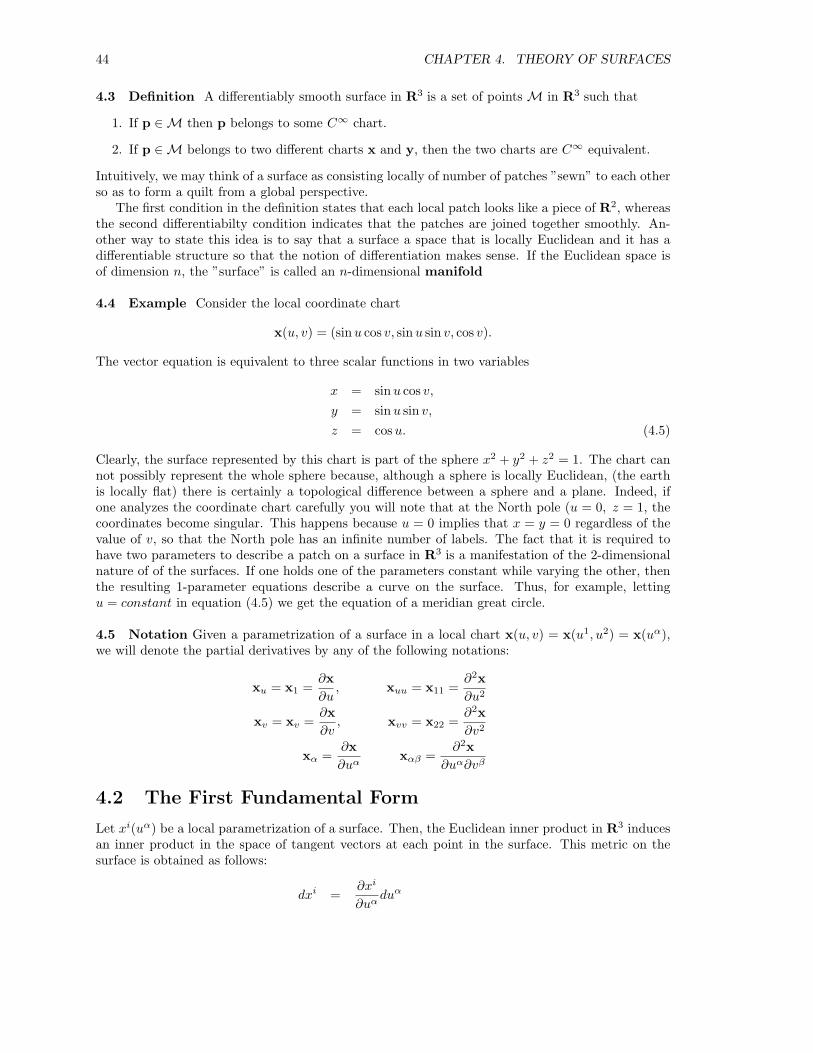
44 CHAPTER 4. THEORY OF SURFACES

4.3 Definition A differentiably smooth surface in R3 is a set of points M in R3 such that

1. If p ∈M then p belongs to some C∞ chart.

2. If p ∈M belongs to two different charts x and y, then the two charts are C∞ equivalent.

Intuitively, we may think of a surface as consisting locally of number of patches ”sewn” to each otherso as to form a quilt from a global perspective.

The first condition in the definition states that each local patch looks like a piece of R2, whereasthe second differentiabilty condition indicates that the patches are joined together smoothly. An-other way to state this idea is to say that a surface a space that is locally Euclidean and it has adifferentiable structure so that the notion of differentiation makes sense. If the Euclidean space isof dimension n, the ”surface” is called an n-dimensional manifold

4.4 Example Consider the local coordinate chart

x(u, v) = (sinu cos v, sinu sin v, cos v).

The vector equation is equivalent to three scalar functions in two variables

x = sinu cos v,y = sinu sin v,z = cosu. (4.5)

Clearly, the surface represented by this chart is part of the sphere x2 + y2 + z2 = 1. The chart cannot possibly represent the whole sphere because, although a sphere is locally Euclidean, (the earthis locally flat) there is certainly a topological difference between a sphere and a plane. Indeed, ifone analyzes the coordinate chart carefully you will note that at the North pole (u = 0, z = 1, thecoordinates become singular. This happens because u = 0 implies that x = y = 0 regardless of thevalue of v, so that the North pole has an infinite number of labels. The fact that it is required tohave two parameters to describe a patch on a surface in R3 is a manifestation of the 2-dimensionalnature of of the surfaces. If one holds one of the parameters constant while varying the other, thenthe resulting 1-parameter equations describe a curve on the surface. Thus, for example, lettingu = constant in equation (4.5) we get the equation of a meridian great circle.

4.5 Notation Given a parametrization of a surface in a local chart x(u, v) = x(u1, u2) = x(uα),we will denote the partial derivatives by any of the following notations:

xu = x1 =∂x∂u, xuu = x11 =

∂2x∂u2

xv = xv =∂x∂v, xvv = x22 =

∂2x∂v2

xα =∂x∂uα

xαβ =∂2x

∂uα∂vβ

4.2 The First Fundamental Form

Let xi(uα) be a local parametrization of a surface. Then, the Euclidean inner product in R3 inducesan inner product in the space of tangent vectors at each point in the surface. This metric on thesurface is obtained as follows:

dxi =∂xi

∂uαduα

4.2. THE FIRST FUNDAMENTAL FORM 45

ds2 = δijdxidxj

= δij∂xi

∂uα

∂xj

∂uβduαduβ .

Thus,ds2 = gαβdu

αduβ , (4.6)

where

gαβ = δij∂xi

∂uα

∂xj

∂uβ. (4.7)

We conclude that the surface, by virtue of being embedded in R3 , inherits a natural metric (4.6)which we will call the induced metric. A pair M, g, whereM is a manifold and g = gαβdu

α⊗duβ

is a metric is called a Riemannian manifold if considered as an entity in itself, and Riemanniansubmanifold of Rn if viewed as an object embedded in Euclidean space. An equivalent version ofthe metric (4.6) can be obtained by using a more traditional calculus notation

dx = xudu+ xvdv

ds2 = dx · dx= (xudu+ xvdv) · (xudu+ xvdv)= (xu · xu)du2 + 2(xu · xv)dudv(xv · xv)dv2.

We can rewrite the last result as

ds2 = Edu2 + 2Fdudv +Gdv2, (4.8)

where

E = g11 = xu · xu

F = g12 = xu · xv

= g21 = xv · xu

G = g22 = xv · xv.

That isgαβ = xα · xβ =< xα,xβ > .

4.6 bdf The element of arclengthds2 = gαβdu

α ⊗ duβ (4.9)

is also called the first fundamental form. We must caution the reader that this quantity is nota form in the sense of differential geometry since ds2 involves the symmetric tensor product ratherthan the wedge product.

The first fundamental form plays such a crucial role in the theory of surfaces, that will find itconvenient to introduce yet a third more modern version. Following the same development as in thetheory of curves, consider a surface M defined locally by a function (u1, u2) 7−→ α(u1, u2). We saythat a quantity Xp is a tangent vector at a point p ∈M, if Xp is a linear derivation on the space ofC∞ real-valued functions f |f : M−→ R on the surface. The set of all tangent vectors at a pointp ∈ M is called the tangent space TpM. As before, a vector field X on the surface is a smoothchoice of a tangent vector at each point on the surface and the union of all tangent spaces is calledthe tangent bundle TM.

The coordinate chart mapα : R2 −→M ∈ R3


induces a push-forward mapα∗ : TR2 −→ TM

defined byα∗(V )(f) |α(uα)= V (α f) |uα

Just as in the case of curves, when we revert back to classical notation to describe a surface asxi(uα), what we really mean is (xi α)(uα), where x1 are the coordinate functions in R3 . Particularexamples of tangent vectors on M are given by the push-forward of the standard basis of TR2.These tangent vectors which earlier we called xα are defined by

α∗(∂

∂uα)(f) |α(uα)=

∂

∂uα(α f) |uα

In this formalism, the first fundamental form I is just the symmetric bilinear tensor defined byinduced metric

I(X,Y ) = g(X,Y ) =< X,Y >, (4.10)

where X and Y are any pair of vector fields in TM.

Orthogonal Parametric Curves

Let V and W be vectors tangent to a surface M defined locally by a chart x(uα). Since the vectorsxalpha span the tangent space of M at each point, the vectors V and W can be written as linearcombinations

V = V αxα

W = Wαxα.

The functions V α and Wα are called the curvilinear coordinates of the vectors. We can calculatethe length and the inner product of the vectors using the induced Riemannian metric,

‖V ‖2 = < V, V >=< V αxα, Vβxβ >= V αV β < xα,xβ >

‖V ‖2 = gαβVαV β

‖W‖2 = gαβWαW β ,

and

< V,W > = < V αxα,Wβxβ >= V αW β < xα,xβ >

= gαβVαW β .

The angle θ subtended by the the vectors v and W is the given by the equation

cos θ =< V,W >

‖V ‖ · ‖W‖

=I(V,W )√

I(V, V )√I(W,W )

=gαβV

αW β

gαβV αV β · gαβWαW β. (4.11)

Let uα = φα(t) and uα = ψα(t) be two curves on the surface. Then the total differentials

duα =dφα

dtdt, and δuα =

dψα

dtδt

4.2. THE FIRST FUNDAMENTAL FORM 47

represent infinitesimal tangent vectors (1.12) to the curves. Thus, the angle between two infinitesimalvectors tangent to two intersecting curves on the surface satisfies

cos θ =gαβdu

αδuβ√gαβduαduβ

√gαβδuαδuβ

(4.12)

In particular, if the two curves happen to be the parametric curves, u1 = constant and u2 =constant then along one curve we have du1 = 0, du2 arbitrary, and along the second we have δu1

arbitrary and δu2 = 0. In this case, the cosine of the angle subtended by the infinitesimal tangentvectors reduces to

cos θ =g12δu

1du2√g11(δu1)2

√g22(du2)2

=g12

g11g22=

F√EG

. (4.13)

As a result, we have the following

4.7 Proposition The parametric lines are orthogonal if F = 0.

4.8 Examplesa) Sphere

x = (a sin θ cosφ, a sin θ sinφ, a cos θ)xθ = (a cos θ cosφ, a cos θ sinφ,−a sin θ)xφ = (−a sin θ sinφ, a sin θ cosφ, )E = xθ · xθ = a2

F = xθ · xφ = 0G = xφ · xφ = a2 sin2 θ

ds2 = a2dθ2 + a2 sin2 θdφ2

b) Surface of Revolution

x = (r cos θ, r sin θ, f(r))xr = (cos θ, sin θ, f ′(r))xθ = (−r sin θ, r cos θ, 0)E = xr · xr = 1 + f ′2(r)F = xr · xθ = 0G = xθ · xθ = r2

ds2 = [1 + f ′2(r)]dr2 + r2dθ2

c) Pseudosphere

x = (a sinu cos v, a sinu sin v, a(cosu ln tanu

2))

E = a2 cot2 uF = = 0G = a2 sin2 u

ds2 = a2 cot2 udu2 + a2 sin2 udv2

d) Torus


x = ((b+ a cosu) cos v, (b+ a cosu) sin v, a sinu)E = a2

F = 0G = (b+ a cosu)2

ds2 = a2du2 + (b+ a cosu)2dv2

e) Helicoid

x = (u cos v, u sin v, av)E = 1F = 0G = u2 + a2

ds2 = du2 + (u2 + a2)dv2

f) Catenoid

x = (u cos v, u sin v, c cosh−1 u

c)

E =u2

u2 − c2

F = 0G = u2

ds2 =u2

u2 − c2du2 + u2dv2

4.3 The Second Fundamental Form

Let x = x(uα) be a coordinate patch on a surface M. Since xu and xv are tangential to the surface,we can construct a unit normal n to the surface by taking

n =xu × xv

‖xu × xv‖(4.14)

Now, consider a curve on the surface given by uα = uα(s). Without loss of generality, we assumethat the curve is parametrized by arclength s so that the curve has unit speed. Using the chain rule,we se that the unit tangent vector T to the curve is given by

T =dxds

=dxduα

duα

ds= xα

duα

ds(4.15)

Since the curve lives on the surface and the the vector T is tangent to the curve, it is clear thatT is also tangent to the surface. On the other hand, the vector T ′ = dT/ds does not in general havethis property, so what we will do is to decompose T ′ into its normal and tangential components (seefig (4.2))

T ′ = Kn +Kg

= κnn +Kg, (4.16)

where κn = ‖Kn‖ =< T ′,n >The scalar quantity κn is called the normal curvature of the curve and Kg is called the

geodesic curvature vector. The normal curvature measures the the curvature of x(uα(s)) resulting

4.3. THE SECOND FUNDAMENTAL FORM 49

Figure 4.2: Normal Curvature

by the constraint of the curve to lie on a surface. The geodesic curvature vector , measures the“sideward” component of the curvature in the tangent plane to the surface. Thus, if one draws astraight line on a flat piece of paper and then smoothly bend the paper into a surface, then thestraight line would now acquire some curvature. Since the line was originally straight, there is nosideward component of curvature so Kg = 0 in this case. This means that the entire contributionto the curvature comes from the normal component, reflecting the fact that the only reason there iscurvature here is due to the bend in the surface itself.

Similarly, if one specifies a point p ∈M and a direction vector Xp ∈ TpM, one can geometricallyenvision the normal curvature by considering the equivalence class of all unit speed curves in Mwhich contain the point p and whose tangent vectors line up with the direction of X. Of course,there are infinitely many such curves, but at an infinitesimal level, all these curves can be obtainedby intersecting the surface with a ”vertical” plane containing the vector X and the normal to M.All curves in this equivalence class have the same normal curvature and their geodesic curvaturesvanish. In this sense, the normal curvature is more of a property pertaining to a direction on thesurface at a point, whereas, the geodesic curvature really depends on the curve itself. It might beimpossible for a hiker walking on the ondulating hills of the Ozarks to find a straight line trail, sincethe rolling hills of the terrain extend in all directions. However, it might be possible to walk on apath with zero geodesic curvature as long as the hiker can maintain the same compass direction.

To find an explicit formula for the normal curvature we first differentiate equation (4.15)

T ′ =dT

ds

=d

ds(xα

duα

ds)

=d

ds(xα)

duα

ds+ xα

d2uα

ds2

= (dxα

duβ

duβ

ds)duα

ds+ xα

d2uα

ds2

= xαβduα

ds

duβ

ds+ xα

d2uα

ds2.

Taking the inner product of the last equation with the normal and noticing that < xα,n >= 0, weget

κn = < T ′,n >=< xαβ ,n >duα

ds

duβ

ds

=bαβdu

αduβ

gαβduαduβ, (4.17)

wherebαβ =< xαβ ,n > (4.18)

4.9 Definition The expressionII = bαβdu

α ⊗ duβ (4.19)

is called the second fundamental form .


4.10 Proposition The second fundamental form is symmetric.Proof: In the classical formulation of the second fundamental form the proof is trivial. We havebαβ = bβα since for a C∞ patch x(uα), we have xαβ = xβα because the partial derivatives commute.

We will denote the coefficients of the second fundamental form by

e = b11 =< xuu,n >

f = b12 =< xuv,n >

= b21 =< xvu,n >

g = b22 =< xvv,n >

, so that equation (4.19) can be written as

II = edu2 + 2fdudv + gdv2 (4.20)

and equation (4.17) as

κn =II

I=Edu2 + 2Fdudv +Gdv2

edu2 + 2fdudv + gdv2(4.21)

We would also like to point out that just as the first fundamental form can be represented as

I =< dx, dx >,

so can we represent the second fundamental form as

II = − < dx, dn >

To see this it suffices to note that differentiation of the identity < xα,n >= 0 implies that

< xαβ ,n >= − < xα,nβ > .

Therefore,

< dx, dn > = < xαduα,nβdu

β >

= < xαduα,nβdu

β >

= < xα,nβ > duαduβ

= − < xαβ ,n > duαduβ

= −II

From a computational point a view, a more useful formula for the coefficients of the secondfundamental formula can be derived by first applying the classical vector identity

(A×B) · (C ×D) =∣∣∣∣ A · C A ·DB · C B ·D

∣∣∣∣ (4.22)

to compute

‖xu × xv‖2 = (xu × xv) · (xu × xv)

= det

[xu · xu xu · xv

xv · xu xv · xv

]= EG− F 2 (4.23)

Consequently, the normal vector can be written as

n =xu × xv

‖xu × xv‖=

xu × xv√EG− F 2

4.4. CURVATURE 51

Thus, we can write the coefficients bαβ directly as triple products involving derivatives of (x). Theexpressions for these coefficients are

e =(xuxuxuu)√EG− F 2

f =(xuxvxuv)√EG− F 2

g =(xvxvxvv)√EG− F 2

(4.24)

The first fundamental form on a surface measures the (square) of the distance between twoinfinitesimally separated points. There is a similar interpretation of the second fundamental formas we show below. The second fundamental form measures the distance from a point on the surfaceto the tangent plane at a second infinitesimally separated point. To see this simple geometricalinterpretation, consider a point x0 = x(uα

0 ) ∈M and a nearby point x(uα0 + duα). Expanding on a

Taylor series, we get

x(uα0 + duα) = x0 + (x0)αdu

α +12(x0)αβdu

αduβ + . . .

We recall that the distance formula from a point x to a plane which contains x0 is just the scalarprojection of (x− x0) onto the normal. Since the normal to the plane at x0 is the same as the unitnormal to the surface and < xα,n >= 0, we find that the distance D is

D = < x− x0,n >

=12< (x0)αβ ,n > duαduβ

=12II0

The first fundamental form (or rather, its determinant) also appears in calculus in the contextof calculating the area of a parametrized surface. the reason is that if one considers an infinitesimalparallelogram subtended by the vectors xudu and xvdv, then the differential of surface area is givenby the length of the cross product of these two infinitesimal tangent vectors. That is

dS = ‖xu × xv‖ dudv

S =∫ ∫ √

EG− F 2 dudv

The second fundamental form contains information about the shape of the surface at a point.For example, the discussion above indicates that if b = |bαβ | = eg − f2 > 0 then all the neighboringpoints lie on the same side of the tangent plane, and hence, the surface is concave in one direction.If at a point on a surface b > 0, the point is called an elliptic point, if b < 0, the point is calledhyperbolic or a saddle point, and if b = 0, the point is called parabolic.

4.4 Curvature

Curvature and all related questions which surround curvature, constitute the central object of studyin differential geometry. One would like to be able to answer questions such as, what quantitiesremain invariant as one surface is smoothly changed into another? There is certainly somethingintrinsically different from a cone, which we can construct from a flat piece of paper and a spherewhich we can not. What is it that makes these two surfaces so different? How does one calculatethe shortest path between two objects when the path is constrained to be on a surface?


These and many other questions of similar type can be quantitatively answered through thestudy curvature. We cannot overstate the great importance of this subject; perhaps it suffices to saythat without a clear understanding of curvature, there would not be a general theory of relativity,no concept of black holes, and even more disastrous, no Star Trek.

The study of curvature of a hypersurface in Rn (a surface of dimension n−1) begins by trying tounderstand the covariant derivative of the normal to the surface. The reason is simple. If the normalto a surface is constant, then the surface is a flat hyperplane. Thus, it is variations in the normalthat indicate the presence of curvature. For simplicity, we constrain our discussion to surfaces inR3 , but the formalism we use is applicable to any dimension. We will also introduce in this sectionthe modern version of the second fundamental form

4.11 Definition Let X be a vector field on a surface M in R3 , and let N be the normal vector.The map L given by

LX = −∇XN (4.25)

is called the Weingarten map.In this definition we will be careful to differentiate between operators which live on the surface

and operators which live in the ambient space. We will adopt the convention of overlining objectswhich live in the ambient space, the operator ∇ above being an example of one such object. TheWeingarten map is clearly a good place to start, since it is the rate of change of the normal in anarbitrary direction which we wish to quantify.

4.12 Definition The Lie bracket [X,Y ] of two vector fields X and Y on a surface M is definedas the commutator

[X,Y ] = XY = Y X, (4.26)

meaning that if f is a function on M then [X,Y ]f = X(Y (f))− Y (X(f)).

4.13 Proposition The Lie bracket of two vectors X,Y ∈ T (calM) is another vector in T (M).Proof: If suffices to prove that the bracket is a linear derivation on the space of C∞ functions.Consider vectors X,Y ∈ T (calM) and smooth functions f, g in M. Then

[X,Y ](f + g) = X(Y (f + g))− Y (X(f + g))= X(Y (f) + Y (g))− Y (X(f) +X(g))= X(Y (f))− Y (X(f)) +X(Y (g))− Y (X(g))= [X,Y ](f) + [X,Y ](g),

[X,Y ](fg) = X(Y (fg))− Y (X(fg))= X[fY (g) + gY (f)]− Y [fX(g) + gX(f)]= X(f)Y (g) + fX(Y (g)) +X(g)Y (f) + gX(Y (f))

−Y (f)X(g)− f(Y (X(g))− Y (g)X(f)− gY (X(f))= f [X(Y (g))− (Y (X(g))] + g[X(Y (f))− Y (X(f))]= f [X,Y ](g) + g[X,Y ](f).

4.14 Proposition The Weingarten map is a linear transformation on T (M).Proof: Linearity follows from the linearity of ∇, so it suffices to show that L : X −→ LX mapsX ∈ T (M) to a vector LX ∈ T (M). Since N is the unit normal to the surface, < N,N >= 1, sothat any derivative of < N,N > is 0. Assuming that the connection is compatible with the metric,

4.4. CURVATURE 53

∇X < N,N > = < ∇XN,> + < N,∇XN >

= 2 < ∇XN,N >

= 2 < LX,N >= 0.

Therefore, LX is orthogonal to N , and hence it lies in T (M).We recall at this point that the in the previous section we gave two equivalent definitions <

dx, dx >, and < X,Y >) of the first fundamental form. We will now do the same for the secondfundamental form.

4.15 Definition The second fundamental form is the bilinear map

II(X,Y ) =< LX, Y > (4.27)

4.16 Remark It should be noted that the two definitions of the second fundamental form areconsistent. This is easy to see if one chooses X to have components xα and Y to have componentsxβ . With these choices, LX has components −na and II(X,Y ) becomes bαβ = − < xα,nβ > Wealso note that there is third fundamental form defined by

III(X,Y ) =< LX,LY >=< L2X,Y > (4.28)

In classical notation, the third fundamental form would be denoted by < dn, dn >. As one wouldexpect, the third fundamental form contains third order Taylor series information about the surface.We will not treat III(X,Y ) in much detail in this work.

4.17 Definition The torsion of a connection ∇ is the operator T such that ∀X,Y

T (X,Y ) = ∇XY −∇Y X − [X,Y ] (4.29)

A connection is called torsion free if T (X,Y ) = 0. In this case,

∇XY −∇Y X = [X,Y ].

We will say much more later about the torsion and the importance of torsion free connections.For the time being, it suffices to assume that for the rest of this section, all connections are torsionfree. Using this assumption, it is possible to prove the following very important theorem.

4.18 Theorem The Weingarten map is a self adjoint operator on TM.Proof: We have already shown that L : TM −→ TM is a linear map. Recall that an operatorL on a linear space is self adjoint if < LX,Y >=< X,LY >, so that the theorem is equivalent toproving that that the second fundamental for is symmetric (II[X,Y ] = II[Y,X]). Computing thedifference of these two quantities, we get

II[X,Y ]− II[Y,X] = < LX, Y > − < LY,X >

= < ∇XN,Y > − < ∇Y N,X > .

Since < X,N >=< Y,N >= 0, and the connection is compatible with the metric, we know that

< ∇XN,Y > = − < N,∇XY >

< ∇Y N,X > = − < N,∇Y X >,


hence,

II[X,Y ]− II[Y,X] = < N,∇Y X > − < N,∇XY >,

= < N,∇Y X −∇XY >

= < N, [X,Y ] >= 0 (iff [X,Y ] ∈ T (M))

One of the most important topics in an introductory course linear algebra deals with the spectrumof self adjoint operators. The main result in this area states that if one considers the eigenvalueequation

LX = κX (4.30)

then the eigenvalues are always real and eigenvectors corresponding to different eigenvalues are or-thogonal. In the current situation, the vector spaces in question are the tangent spaces at each pointof a surface in R3 , so the dimension is 2. Hence, we expect two eigenvalues and two eigenvectors

LX1 = κ1X1 (4.31)LX2 = κ1X2. (4.32)

4.19 Definition The eigenvalues κ1 and κ2 of the Weingarten map L are called the principalcurvatures and the eigenvectors X1 and X2 are called the principal directions.

Several possible situations may occur depending on the classification of the eigenvalues at eachpoint p on the surface:

1. If κ1 6= κ2 and both eigenvalues are positive, then p is called an elliptic point

2. If κ1κ2 < 0, then p is called a hyperbolic point.

3. If κ1 = κ2 6= 0, then p is called an umbilic point.

4. if κ1κ2 = 0, then p is called a parabolic point

It is also well known from linear algebra, that the the determinant and the trace of a self adjointoperator are the only invariants under a adjoint (similarity) transformation. Clearly these invariantsare important in the case of the operator L, and they deserve to be given special names.

4.20 Definition The determinant K = det(L) is called the Gaussian curvature of M andH = (1/2)Tr(L) is called the mean curvature.

Since any self-adjoint operator is diagonalizable and in a diagonal basis, the matrix representingL is diag(κ1, κ2), if follows immediately that

K = κ1κ2

H =12(κ1 + κ2) (4.33)

4.21 Proposition Let X and Y be any linearly independent vectors in T (M). Then

LX × LY = K(X × Y )(LX × Y ) + (X × LY ) = 2H(X × Y ) (4.34)

Proof: Since LX,LY ∈ T (M), they can be expresses as linear combinations of the basis vectorsX and Y .

4.4. CURVATURE 55

LX = a1X + b1Y

LY = a2X + b2Y.

computing the cross product, we get

LX × LY =∣∣∣∣ a1 b1a2 b2

∣∣∣∣X × Y

= det(L)(X × Y ).

Similarly

(LX × Y ) + (X × LY ) = (a1 + b2)(X × Y )= Tr(L)(X × Y )= (2H)(X × Y ).

4.22 Proposition

K =eg − f2

EG− F 2

H =12Eg − 2Ff + eG

EG− F 2(4.35)

Proof: Starting with equations (4.34) take the dot product of both sides with X × Y and use thevector identity (4.22). We immediately get

K =

∣∣∣∣ < LX,X > < LX, Y >< LY,X > < LX,X >

∣∣∣∣∣∣∣∣ < X,X > < X,Y >< Y,X > < Y, Y >

∣∣∣∣2H =

∣∣∣∣ < LX,X > < LX, Y >< Y,X > < Y, Y >

∣∣∣∣ +∣∣∣∣ < X,X > < X,Y >< LY,X > < LY, Y >

∣∣∣∣∣∣∣∣ < X,X > < X,Y >< Y,X > < Y, Y >

∣∣∣∣The result follows by taking X = xu and Y = xv

4.23 Theorem (Euler) LetX1 andX2 be unit eigenvectors of L and letX = (cos θ)X1+(sin θ)X2.Then

II(X,X) = κ1 cos2 θ + κ2 sin2 θ (4.36)

Proof: Easy. Just compute II(X,X) =< LX,X >, using the fact the LX1 = κ1X1 , LX2 = κ2X2,and noting that the eigenvectors are orthogonal. We get,

< LX,X > = < (cos θ)κ1X1 + (sin θ)κ2X2, (cos θ)X1 + (sin θ)X2 >

= κ1 cos2 θ < X1, X1 > +κ2 sin2 θ < X2, X2 >

= κ1 cos2 θ + κ2 sin2 θ.

diﬀerential geometry in physicspeople.uncw.edu/lugo/courses/diffgeom/dg1.pdf · diﬀerential...

Documents