differential equations, difference equations and fuzzy ... · differential equations, difference...

JET 39

JET Volume 9 (2016) p.p. 39-54Issue 2, August 2016

Typology of article 1.01www.fe.um.si/en/jet.html

DIFFERENTIAL EQUATIONS, DIFFERENCE EQUATIONS AND FUZZY LOGIC

IN CONTROL OF DYNAMIC SYSTEMS

DIFERENCIALNE ENAČBE, DIFERENČNE ENAČBE IN MEHKA LOGIKA

V UPRAVLJANJU DINAMIČNIH SISTEMOV Janez UsenikR

Keywords: dynamic system, differential equations, Laplace transform, difference equations, z-transform, fuzzy logic

AbstractIn this article, the use of certain mathematical tools to create a dynamic system control is described; such a control could be applied to a power supply system. In continuous dynamic systems, the control of the system is described by one or more differential equations; however, in discrete dynamic sys-tems, this control is described by one or more difference equations. Both differential and difference equations are highly effective tools in conventional mathematical analysis. In the previous twenty years, algorithmic principles of fuzzy logic in the control of the dynamic systems have been very use-ful. In this article, the applications of all three approaches are presented. In the case of the fuzzy logic approach, there is an example of the energy efficiency in the employment of biomass with an empha-sis on developing the environmental sustainable biomass index.

PovzetekV članku so predstavljene matematične metode pri kreiranju upravljanja sinamičnega sistema, ki je lahko tudi energetski sistem. V primeru dinamičnih sistemov je upravljanje opisano z eno ali več diferencialnimi enačbami, v primeru diskretnih sistemov pa je njihovo upravljanje opisano z eno ali več diferenčnimi enačbami.

R Corresponding author: Prof. Janez Usenik, PhD, University of Maribor, Faculty of Energy Technology, Hočevarjev trg 1, SI 8270 Krško, Tel.: +386 40 647 689, E-mail address: [email protected]

40 JET

JET Vol. 9 (2016)Issue 2

Janez Usenik2 Janez Usenik JET Vol. 9 (2016)

Issue 2

‐‐‐‐‐‐‐‐‐‐

Oboje, diferencialne in diferenčne enačbe, so izjemno uporabno orodje v klasični matematični analizi. V zadnjih dvajsetih letih pa se je kot zelo uporabna algoritmična osnova upravljanja dinamičnih sistemov uveljavila uporaba principov mehke logike. Kot hibridni pristop upravljanju dinamičnih sistemov se v zadnjih letih uveljavlja tudi možnost sinteze diferencialnih/diferenčnih enačb ter mehke logike. V članku prikazujemo možnosti uporabe vseh treh pristopov. Za uporabo mehke logike in mehkega sklepanja je podan numerični primer za energetsko izrabo biomase s poudarkom na trajnostnem indeksom varovanja okolja.

1 INTRODUCTION

To solve some technical problems, all the fields of classical mathematics can be used: sets, matrix and vectorial algebra, sequences, series, functions with one and more variables, differential calculus, indefinite integral, definite integral, double, triple and more integrals, line and surface integrals, differential equations, Laplace transform, vector analysis, probability calculus, discrete analysis, difference equations, z‐transform and so on, [1]. In the last fifty years, the technical solutions using fuzzy logic have been very successful [2].

In recent years, as a hybrid approach in the control of the dynamic systems, the option of synthesis of differential/difference equations and fuzzy logic have been made, specifically with regards to fuzzy differential equations [3], [4], [5] and fuzzy difference equations [6], but they still do not have significant applications, and therefore are not considered here.

In this article, the control of the dynamic system by application of differential equations is shown in the first chapter, the application of the difference equation in the second chapter and one application of fuzzy reasoning in the third chapter.

Every model of optimal control is determined by a system, input variables, and the optimality criterion function. The system is represented as a regulation circle, which generally consists of a regulator, a control process, a feedback loop, and input and output information. In this article, only linear dynamic stationary systems will be discussed, [7], [8], [9].

Let us consider a production model in a linear stationary dynamic system in which the input variables indicate the demand for products manufactured by a company. These variables can be a one‐dimensional or multi‐dimensional vector function.

Let us take a stationary random process X with the known mathematical expectation E(X) and autocorrelation RXX(t) as the demand in a stochastic situation that should be met, if possible, by current production. The difference between the current production and demand is the input function for the control process, the output function of which is the current stock/additional capacities. When the difference is positive, the surplus will be stocked, and when it is negative, the demand will also be covered from stock. Of course, in the case of power supply, we do not have stock in the usual sense (such as with cars or computers, etc.); energy cannot be produced in advance for a known customer nor can stock be built up for unknown customers. The demand for energy services is neither uniform in time nor known in advance. It varies, has its ups (peaks) and downs (minima), and it can only be met by installing and activating additional proper technological capacities. Because of this, the function of maintaining stock in the energy supply process belongs to all the additional technological potential/capacities, large enough to meet periods of extra demand. The demand for energy services is not given and precisely known in advance. With market research, we can only learn about the probability of our specific expectations of the intensity of demand. The demand is not given with explicitly expressed

JET 41

Differential equations, difference equations and fuzzy logic in control of dynamic systems Differential equations, difference equations and fuzzy logic in control of dynamic systems 3

‐‐‐‐‐‐‐‐‐‐

mathematical function; we only know the shape and type of the family of functions. Accordingly, demand is a random process for which all the statistical indicators are known.

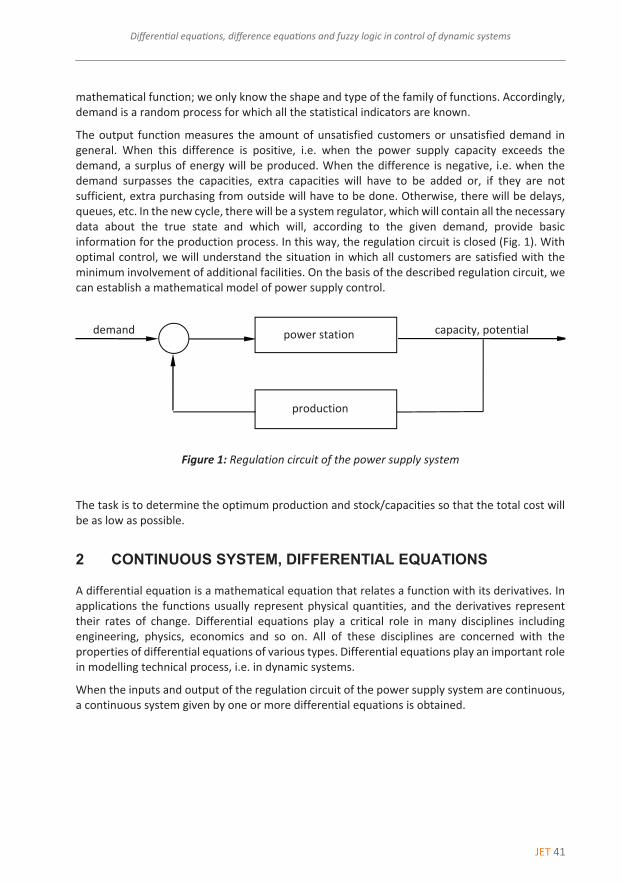
The output function measures the amount of unsatisfied customers or unsatisfied demand in general. When this difference is positive, i.e. when the power supply capacity exceeds the demand, a surplus of energy will be produced. When the difference is negative, i.e. when the demand surpasses the capacities, extra capacities will have to be added or, if they are not sufficient, extra purchasing from outside will have to be done. Otherwise, there will be delays, queues, etc. In the new cycle, there will be a system regulator, which will contain all the necessary data about the true state and which will, according to the given demand, provide basic information for the production process. In this way, the regulation circuit is closed (Fig. 1). With optimal control, we will understand the situation in which all customers are satisfied with the minimum involvement of additional facilities. On the basis of the described regulation circuit, we can establish a mathematical model of power supply control.

Figure 1: Regulation circuit of the power supply system

The task is to determine the optimum production and stock/capacities so that the total cost will be as low as possible.

2 CONTINUOUS SYSTEM, DIFFERENTIAL EQUATIONS

A differential equation is a mathematical equation that relates a function with its derivatives. In applications the functions usually represent physical quantities, and the derivatives represent their rates of change. Differential equations play a critical role in many disciplines including engineering, physics, economics and so on. All of these disciplines are concerned with the properties of differential equations of various types. Differential equations play an important role in modelling technical process, i.e. in dynamic systems.

When the inputs and output of the regulation circuit of the power supply system are continuous, a continuous system given by one or more differential equations is obtained.

demand power station capacity, potential

production

42 JET



Issue 2

‐‐‐‐‐‐‐‐‐‐

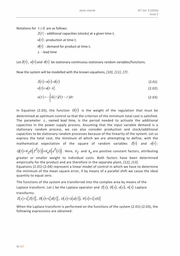
Notations for 0t are as follows: Z t ‐ additional capacities (stocks) at a given time t,

‐ production at time t,

‐ demand for product at time t, ‐ lead time

Let , and be stationary continuous stationary random variables/functions. Now the system will be modelled with the known equations, [10], [11], [7]:

(2.01)

(2.02)

0

t

u t G Z t d (2.03)

In Equation (2.03), the function is the weight of the regulation that must be determined at optimum control so that the criterion of the minimum total cost is satisfied. The parameter , named lead time, is the period needed to activate the additional capacities in the power supply process. Assuming that the input variable demand is a stationary random process, we can also consider production and stock/additional capacities to be stationary random processes because of the linearity of the system. Let us express the total cost, the minimum of which we are attempting to define, with the mathematical expectation of the square of random variables and :

. Here, and are positive constant factors, attributing

greater or smaller weight to individual costs. Both factors have been determined empirically for the product and are therefore in the separate plant, [12], [13]. Equations (2.01)‐(2.04) represent a linear model of control in which we have to determine the minimum of the mean square error, if by means of a parallel shift we cause the ideal quantity to equal zero.

The functions of the system are transferred into the complex area by means of the Laplace transform. Let L be the Laplace operator and Laplace transforms:

When the Laplace transform is performed on the functions of the system (2.01)‐(2.03), the following expressions are obtained:

u t

d t

λ

Z t u t d t

Z t =v t ‐d t

v t =u t ‐ λ

G t

λ

Z t u t

2 2Q t =K E Z t +K E u tuZ KZ Ku

Z s , D s , u s , v s

Z s =L Z t , D s =L d t , U s =L u t , V s =L v(t)

JET 43


‐‐‐‐‐‐‐‐‐‐

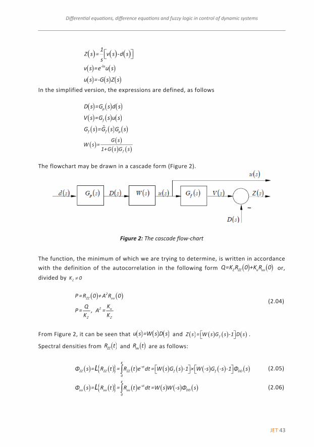
In the simplified version, the expressions are defined, as follows

The flowchart may be drawn in a cascade form (Figure 2).

Figure 2: The cascade flow‐chart

The function, the minimum of which we are trying to determine, is written in accordance with the definition of the autocorrelation in the following form or, divided by

(2.04)

From Figure 2, it can be seen that and .

Spectral densities from and are as follows:

(2.05)

(2.06)

1

Z s = v s ‐d ss

‐λsv s =e u s

u s =‐G s Z s

pD s =G s d s

fV s =G s u s

f f pG s =G s G s

f

G sW s =

1+G s G s

Z ZZ u uuQ=K R 0 +K R 0ZK 0

2ZZ uu

2 u

Z Z

P =R 0 +A R 0

KQP= , A =K K

u s =W s D s fZ s = W s G s ‐1 D s

ZZR t uuR t

¥

‐stZZ ZZ ZZ f f DD

0

Φ s = R t = R t e dt = W s G s ‐1 × W ‐s G ‐s ‐1 Φ sL

¥

‐stuu uu uu DD

0

Φ s = R t = R t e dt =W s W ‐s Φ sL

44 JET



Issue 2

‐‐‐‐‐‐‐‐‐‐

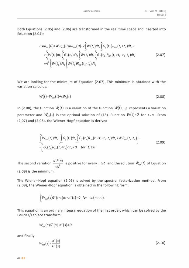
Both Equations (2.05) and (2.06) are transformed in the real time space and inserted into Equation (2.04):

(2.07)

We are looking for the minimum of Equation (2.07). This minimum is obtained with the variation calculus:

(2.08)

In (2.08), the function is a variation of the function , represents a variation

parameter and is the optimal solution of (18). Function for . From (2.07) and (2.08), the Wiener‐Hopf equation is derived

2opt 3 3 f 2 2 f 4 DD 1 2 3 4 4 DD 1 3

‐ ‐ ‐

f 2 DD 1 2 2 1‐

W t dt G t dt G t R t +t ‐t ‐t dt +A R t ‐t ‐

‐ G t R t +t dt =0 for t 0

(2.09)

The second variation is positive for every and the solution of Equation

(2.09) is the minimum. The Wiener‐Hopf equation (2.09) is solved by the spectral factorization method. From (2.09), the Wiener‐Hopf equation is obtained in the following form:

.

This equation is an ordinary integral equation of the first order, which can be solved by the Fourier/Laplace transform:

and finally

(2.10)

¥ ¥2

ZZ uu DD 1 1 f 2 DD 1 2 2‐¥ ‐¥¥ ¥ ¥ ¥

1 1 f 2 2 3 3 f 4 DD 1 2 3 4 4‐¥ ‐¥ ‐¥ ‐¥¥ ¥2

1 1 2 DD 1 2 2‐¥ ‐¥

P =R 0 +A R 0 =R 0 ‐2 W t dt G t R t +t dt +

+ W t dt G t dt W t dt G t R t +t ‐t ‐t dt

+A W t dt W t R t ‐t dt

opt ηW t =W t +ξW t

ηW t W t ξ

optW t W t =0 t < 0

2

2

d P ηdη

1t 0 optW t

+ +opt

‐

W τ Θ t ‐τ dτ ‐π t =0 for t ‐ ,

+ +optW s Θ s ‐π s =0

+

opt +

π sW s =

Θ s

JET 45

Differential equations, difference equations and fuzzy logic in control of dynamic systems

Differential equations, difference equations and fuzzy logic in control of dynamic systems 7

‐‐‐‐‐‐‐‐‐‐

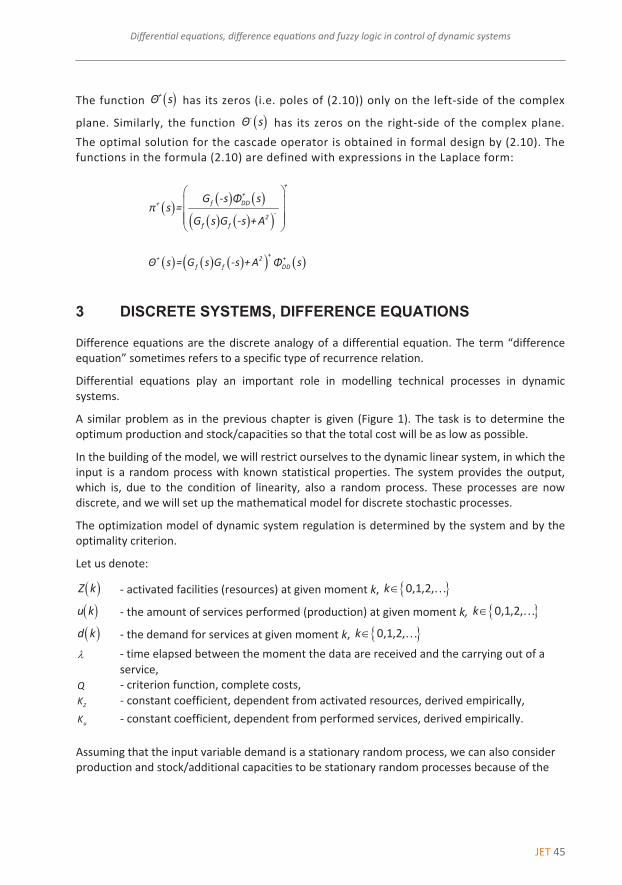
The function has its zeros (i.e. poles of (2.10)) only on the left‐side of the complex

plane. Similarly, the function has its zeros on the right‐side of the complex plane. The optimal solution for the cascade operator is obtained in formal design by (2.10). The functions in the formula (2.10) are defined with expressions in the Laplace form:

3 DISCRETE SYSTEMS, DIFFERENCE EQUATIONS

Difference equations are the discrete analogy of a differential equation. The term “difference equation” sometimes refers to a specific type of recurrence relation.

Differential equations play an important role in modelling technical processes in dynamic systems.

A similar problem as in the previous chapter is given (Figure 1). The task is to determine the optimum production and stock/capacities so that the total cost will be as low as possible.

In the building of the model, we will restrict ourselves to the dynamic linear system, in which the input is a random process with known statistical properties. The system provides the output, which is, due to the condition of linearity, also a random process. These processes are now discrete, and we will set up the mathematical model for discrete stochastic processes.

The optimization model of dynamic system regulation is determined by the system and by the optimality criterion.

Let us denote:

‐ activated facilities (resources) at given moment k,

‐ the amount of services performed (production) at given moment k,

‐ the demand for services at given moment k, ‐ time elapsed between the moment the data are received and the carrying out of a

service, ‐ criterion function, complete costs, ‐ constant coefficient, dependent from activated resources, derived empirically, ‐ constant coefficient, dependent from performed services, derived empirically.

Assuming that the input variable demand is a stationary random process, we can also consider production and stock/additional capacities to be stationary random processes because of the

+Θ s

‐Θ s

++

f DD+‐2

f f

G ‐s Φ sπ s =

G s G ‐s +A

++ 2 +

f f DDΘ s = G s G ‐s + A Φ s

Z k 0,1,2,k

u k 0,1,2,k

d k 0,1,2,k

Q

ZK

uK

46 JET



Issue 2

‐‐‐‐‐‐‐‐‐‐

linearity of the system. Let us consider the functions , and to be discrete stationary random processes. Let the system be formed with these three difference equations, [14]:

(3.01)

(3.02)

(3.03)

Let , , and denote stationary discrete random processes for all

in equations (3.01)–(3.06). Let the autocorrelation of input process be known. For the

criterion of optimality, we shall use a Wiener filter, so we have to determine the minimum of the mean of square error.

(3.04)

Now let us perform a z‐transformation on equations (3.01)‐(3‐03) of our mathematical model. Without loss of generality, it can be assumed that all initial conditions are equal to zero. We then obtain the equations:

If we denote and we can easily calculate

Now we can write:

(3.05)

(3.06)

(3.07)

(3.08)

Z k u k d k

0

PZ k G v k d k

0

fv k G u k

0

u k G Z k

Z k v k u k d k kZ

d k

2 2 2 1Q E Z k A E u k

P PZ z G z v z G z d z

fv z G z u z

u z G z Z z

PD z G z d z f f PG z G z G z

11 f

Z z D zG z G z

u z W z D z

1fZ z W z G z D z fV z G z u z

1 f

G zW z

G z G z

JET 47



‐‐‐‐‐‐‐‐‐‐

With all of these denotations, we can draw a block diagram in cascade form, similar to Figure 2, but all functions are discrete functions. If we denote and , we can also write the optimality criterion

(3.09)

To obtain a shorter and clearer form, take and write expression (3.06) as:

Spectral densities of autocorrelations and are:

Now, let us transform these two equations in the time zone and insert them in (3.09). Since

for , we have

(3.10)

From (3.10), we can calculate the optimum, using a calculus of variations. First, we suppose that solution exists and after that fix

(3.11)

In (3.11), expression is a possible weight, which represents the response of a given system

to input signals; therefore, it means a variation of function , is calling variation parameter,

which can be changed with regard to conditions, while is a solution of equation (3.10). Functions and have to meet the causality condition, meaning for .

If we write (3.11) in optimality criterion (3.10), then and

2 0ZZE Z k R 2 0uuE u k R

20 0ZZ uuP R A R

fS z G z D z

Z z W z S z D z

ZZR k uuR k

1 1ZZ ZZ SS SD SD DDz R k W z W z z W z z W z z z Z 1

uu uu DDz R k W z W z z Z

0W k 0k

2

2

0 0 0 0 0

0 0

2 0

ZZ uu

SS SD DD DDk j k k j

P R A R

W k W j R k j W k R k R A W k W j R k j

optW t

optW t W t W t

W t

W t

optW t

W t W t 0W k 0k

P =P η

48 JET



Issue 2

‐‐‐‐‐‐‐‐‐‐

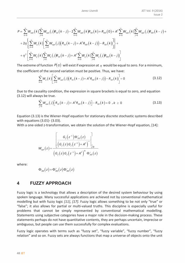
The extreme of function will exist if expression at would be equal to zero. For a minimum, the coefficient of the second variation must be positive. Thus, we have:

(3.12)

Due to the causality condition, the expression in square brackets is equal to zero, and equation (3.12) will always be true.

, (3.13)

Equation (3.13) is the Wiener‐Hopf equation for stationary discrete stochastic systems described with equations (3.01)‐ (3.03). With a one‐sided z‐transformation, we obtain the solution of the Wiener‐Hopf equation, [14]:

where:

4 FUZZY APPROACH

Fuzzy logic is a technology that allows a description of the desired system behaviour by using spoken language. Many successful applications are achieved not by conventional mathematical modelling but with fuzzy logic [11], [17]. Fuzzy logic allows something to be not only “true” or “false”; it also allows for partial or multi‐valued truths. This discipline is especially useful for problems that cannot be simply represented by conventional mathematical modelling. Statements using subjective categories have a major role in the decision‐making process. These statements perhaps do not have quantitative contents, they are perhaps uncertain, imprecise or ambiguous, but people can use them successfully for complex evaluations.

Fuzzy logic operates with terms such as “fuzzy set”, “fuzzy variable”, “fuzzy number”, “fuzzy relation” and so on. Fuzzy sets are always functions that map a universe of objects onto the unit

2opt opt opt opt opt

0 0 0 0 0

2opt

0 0

2 2

0 0 0 0

2 0

2

SS SD DD DDk j k k j

SS DD SDk j

SS DDk j k j

P W k W j R k j W k R k R A W k W j R k j

W k W j R k j A R k j R k

W k W j R k j A W k W j R k j

P

2opt

0 0

0SS DD SDk j

W k W j R k j A R k j R k

2opt

0

0SS DD SDj

W j R k j A R k j R k

0k

1

1 2

1 2

f DD

f f

opt

f f DD

G z z

G z G z AW z

G z G z A z

DD DD DDz z z

JET 49


‐‐‐‐‐‐‐‐‐‐

interval [0, 1]. The degree of membership in a fuzzy set A becomes the degree of truth or a statement and is expressed by a continuous membership function.

The combination of imprecise logic rules in a single control strategy is called approximate or fuzzy reasoning (inference). Thus, the fuzzy inference is the process of formulating the mapping from a given input to an output using fuzzy logic.

In principle, every system can be modelled, analysed and solved by means of fuzzy logic. Due to the complexity of the given problem and the subjective decisions of customers, which are better described with fuzzy reasoning, it is advisable to introduce a fuzzy approach. Some basic solutions of the control problems using fuzzy reasoning were presented by other researchers [10], [12]. For some problems about the control of the dynamic system, we propose fuzzy reasoning.

Construction of a fuzzy system takes several steps: selection of decision variables and their fuzzification, establishing the goal, and the construction of an algorithm (base of rules of fuzzy reasoning), inference, and defuzzification of the results of fuzzy inference.

The output of a fuzzy process can be the logical union of two or more fuzzy membership functions defined on the universe of discourse of the output variable. Defuzzification is the conversion of a given fuzzy quantity to a precise, crisp quantity. Our model is created with FuzzyTech 5.55i software, and we use the Centre of Maximum (CoM) defuzzification method.

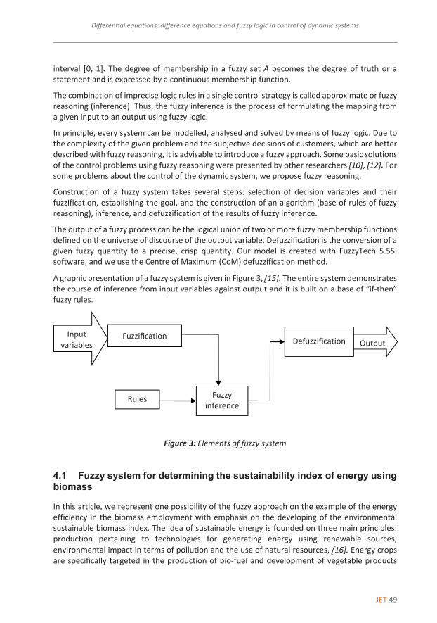
A graphic presentation of a fuzzy system is given in Figure 3, 15]. The entire system demonstrates the course of inference from input variables against output and it is built on a base of “if‐then” fuzzy rules.

Figure 3: Elements of fuzzy system

4.1 Fuzzy system for determining the sustainability index of energy using biomass

In this article, we represent one possibility of the fuzzy approach on the example of the energy efficiency in the biomass employment with emphasis on the developing of the environmental sustainable biomass index. The idea of sustainable energy is founded on three main principles: production pertaining to technologies for generating energy using renewable sources, environmental impact in terms of pollution and the use of natural resources, 16]. Energy crops are specifically targeted in the production of bio‐fuel and development of vegetable products

Input variables

Fuzzification

Fuzzy inference

Defuzzification Output

Rules

50 JET



Issue 2

‐‐‐‐‐‐‐‐‐‐

suitable for industrial processing and transformation into energy. The procedure of measuring sustainability is very complex, and it must operate with attributes that are not defined precisely in most cases. For such problems, the proper choice is the use of fuzzy logic, which deals with uncertainty in environmental topics. Following 16] and generalizing it, in this chapter, a fuzzy system to determine the sustainability of production and use of biomass for energy purposes is proposed.

In the building the fuzzy system based on the fuzzy inference, we have to make these steps: fuzzification, fuzzy inference (rules, algorithm), defuzzification and optimization.

4.1.1 Fuzzification

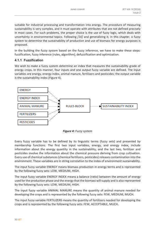
We wish to make a fuzzy system determine an index that measures the sustainability grade of energy crops. In this manner, four inputs and one output fuzzy variable are defined. The input variables are energy, energy index, animal manure, fertilizers and pesticides; the output variable is the sustainability index (Figure 4).

Figure 4: Fuzzy system

Every fuzzy variable has to be defined by its linguistic terms (fuzzy sets) and presented by membership functions. The first two input variables, energy, and energy index, include information about the energy quantity in the sustainability, and the last two, fertilizer and pesticides involve the information about the chemical pressure deriving from crop cultivation. Every use of chemical substances (chemical fertilizers, pesticides) releases contamination into the environment. These variables are in string correlation to the index of environment sustainability.

The input fuzzy variable ENERGY means biomass production in energy terms and is represented by the following fuzzy sets: LOW, MEDIUM, HIGH.

The input fuzzy variable ENERGY INDEX means a balance (ratio) between the amount of energy used for the production phase and the energy that the biomass will supply and is also represented by the following fuzzy sets: LOW, MEDIUM, HIGH.

The input fuzzy variable ANIMAL MANURE means the quantity of animal manure needed for developing the crops and is represented by the following fuzzy sets: FEW, MEDIUM, MUCH.

The input fuzzy variable FERTILIZERS means the quantity of fertilizers needed for developing the crops and is represented by the following fuzzy sets: FEW, ACCEPTABLE, MUCH.

JET 51



‐‐‐‐‐‐‐‐‐‐

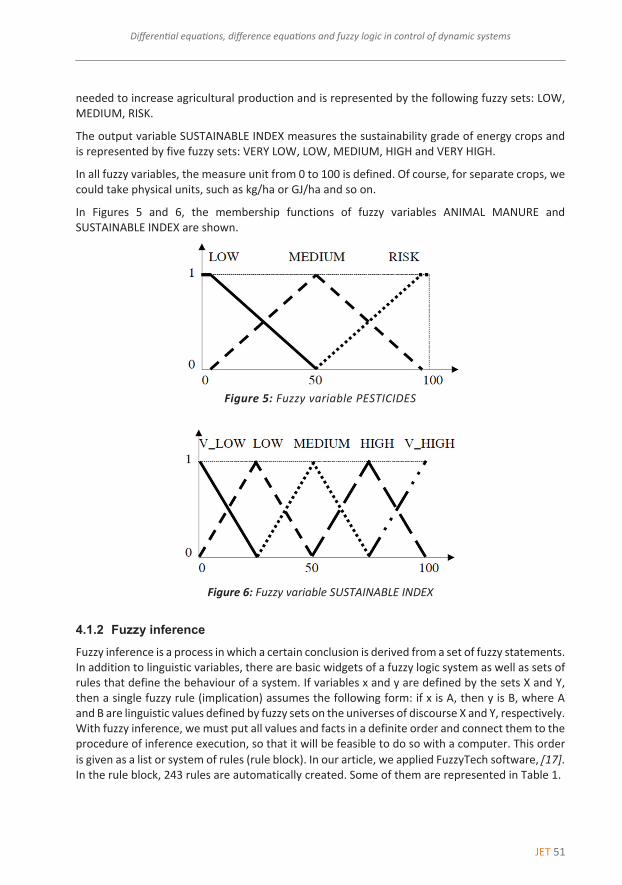
The input fuzzy variable PESTICIDES means the quantity of dangerous chemical substances needed to increase agricultural production and is represented by the following fuzzy sets: LOW, MEDIUM, RISK.

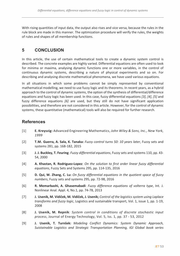
The output variable SUSTAINABLE INDEX measures the sustainability grade of energy crops and is represented by five fuzzy sets: VERY LOW, LOW, MEDIUM, HIGH and VERY HIGH.

In all fuzzy variables, the measure unit from 0 to 100 is defined. Of course, for separate crops, we could take physical units, such as kg/ha or GJ/ha and so on.

In Figures 5 and 6, the membership functions of fuzzy variables ANIMAL MANURE and SUSTAINABLE INDEX are shown.

Figure 5: Fuzzy variable PESTICIDES

Figure 6: Fuzzy variable SUSTAINABLE INDEX

4.1.2 Fuzzy inference

Fuzzy inference is a process in which a certain conclusion is derived from a set of fuzzy statements. In addition to linguistic variables, there are basic widgets of a fuzzy logic system as well as sets of rules that define the behaviour of a system. If variables x and y are defined by the sets X and Y, then a single fuzzy rule (implication) assumes the following form: if x is A, then y is B, where A and B are linguistic values defined by fuzzy sets on the universes of discourse X and Y, respectively. With fuzzy inference, we must put all values and facts in a definite order and connect them to the procedure of inference execution, so that it will be feasible to do so with a computer. This order is given as a list or system of rules (rule block). In our article, we applied FuzzyTech software, 17]. In the rule block, 243 rules are automatically created. Some of them are represented in Table 1.

52 JET



Issue 2

‐‐‐‐‐‐‐‐‐‐

Table 1: Some rules of the Rule block

IF THEN ANIMAL MAN.

ENERGY ENERGY INDEX FERTILIZERS PESTICIDES SUSTAIN. INDEX

MEDIUM HIGH LOW MUCH LOW MEDIUM MEDIUM HIGH LOW MUCH ACCEPTABLE HIGH MEDIUM HIGH LOW MUCH RISK HIGH MEDIUM HIGH MEDIUM FEW LOW LOW MEDIUM HIGH MEDIUM FEW ACCEPTABLE MEDIUM MEDIUM HIGH MEDIUM FEW RISK MEDIUM MEDIUM HIGH MEDIUM MEDIUM LOW MEDIUM MEDIUM HIGH MEDIUM MEDIUM ACCEPTABLE MEDIUM MEDIUM HIGH MEDIUM MEDIUM RISK HIGH MEDIUM HIGH MEDIUM MUCH LOW MEDIUM MEDIUM HIGH MEDIUM MUCH ACCEPTABLE HIGH MEDIUM HIGH MEDIUM MUCH RISK HIGH MEDIUM HIGH HIGH FEW LOW MEDIUM MEDIUM HIGH HIGH FEW ACCEPTABLE MEDIUM MEDIUM HIGH HIGH FEW RISK HIGH MEDIUM HIGH HIGH MEDIUM LOW MEDIUM MEDIUM HIGH HIGH MEDIUM ACCEPTABLE HIGH

4.1.3 Defuzzification

Defuzzification is the conversion of a given fuzzy output to a precise, crisp output. There are many procedures for defuzzification, which can give some different results. In our example, the fuzzy model is created with FuzzyTech 5.55i software, and we use the Centre of Maximum (CoM) defuzzification method.

4.1.4 Optimisation

When the system structure is set, and the membership functions and rules in all the rule blocks are defined, the model must also be tested and checked. During optimization, the entire definition area of input data is verified.

4.1.5 Numerical example

Starting with the fuzzy model using FuzzyTech software, we can simulate all possible situations interactively. Some numerical results are shown in Table 2.

Table 2: Some numerical results

ANIMAL MAN. ENERGY ENERGY INDEX FERTILIZERS PESTICIDES SUSTAIN. INDEX 10 10 10 50 30 39.2 50 50 50 50 50 50.0 100 50 50 100 100 75.0 80 80 50 10 20 37.6 90 80 80 10 50 43.6 100 30 40 100 80 55.3

JET 53


‐‐‐‐‐‐‐‐‐‐

With rising quantities of input data, the output also rises and vice versa, because the rules in the rule block are made in this manner. The optimization procedure will verify the rules, the weights of rules and shapes of all membership functions.

5 CONCLUSION

In this article, the use of certain mathematical tools to create a dynamic system control is described. The concrete examples are highly varied. Differential equations are often used to look for minima or maxima, analysing dynamic functions one or more variables, in the control of continuous dynamic systems, describing a nature of physical experiments and so on. For describing and analysing discrete mathematical phenomena, we have used various equations.

In all situations in which some problems cannot be simply represented by conventional mathematical modelling, we need to use fuzzy logic and its theorems. In recent years, as a hybrid approach to the control of dynamic systems, the option of the synthesis of differential/difference equations and fuzzy logic has been used. In this case, fuzzy differential equations [3], [4], [5] and fuzzy difference equations [6] are used, but they still do not have significant application possibilities, and therefore are not considered in this article. However, for the control of dynamic systems, these quantitative (mathematical) tools will also be required for further research.

References

[1] E. Kreyszig: Advanced Engineering Mathematics, John Wiley & Sons, Inc., New York, 1999

[2] T.M. Guerra, A. Sala, K. Tanaka: Fuzzy control turns 50: 10 years later, Fuzzy sets and systems 281, pp. 168‐182, 2015

[3] J. J. Buckley, T. Feuring: Fuzzy differential equations, Fuzzy sets and systems 110, pp. 43‐54, 2000

[4] A. Khastan, R. Rodriguez‐Lopez: On the solution to first order linear fuzzy differential equations, Fuzzy Sets and Systems 295, pp. 114‐135, 2016

[5] D. Qui, W. Zhang, C. Lu: On fuzzy differential equations in the quotient space of fuzzy numbers, Fuzzy sets and systems 295, pp. 72‐98, 2016

[6] R. Memarbashi, A. Ghasemabadi: Fuzzy difference equations of volterra type, Int. J. Nonlinear Anal. Appl. 4, No.1, pp. 74‐78, 2013

[7] J. Usenik, M. Vidiček, M. Vidiček, J. Usenik; Control of the logistics system using Laplace transforms and fuzzy logic, Logistics and sustainable transport, Vol. 1, issue 1, pp. 1‐19, 2008

[8] J. Usenik, M. Repnik: System control in conditions of discrete stochastic input process, Journal of Energy Technology, Vol. 5, Iss. 1, pp. 37 ‐ 53, 2012

[9] J. Usenik, T. Turnšek: Modeling Conflict Dynamics: System Dynamic Approach, Suistainable Logistics and Strategic Transportation Planning, IGI Global book series

54 JET



Issue 2

‐‐‐‐‐‐‐‐‐‐

Advanced in Logistics, Operations, and management, Business Science Reference, Hershey PA, USA, pp. 273‐294, 2016

[10] M. Bogataj, J. Usenik. Fuzzy approach to the spatial games in the total market, Int., j. prod. econ., Vol. 93‐94, pp. 493‐503, 2005

[11] D. Kovačič, J. Usenik, M. Bogataj: Optimal decisions on investments in urban energy cogeneration plants ‐ extended MRP and fuzzy approach to the stochastic systems, International journal of production economics, 2016

[12] J. Usenik, M. Bogataj: A fuzzy set approach for a location‐inventory model, Transp. plan. technol., Vol. 28, pp. 447‐464, 2005

[13] J. Usenik: A fuzzy model of power supply system control, JET Journal of Energy technology, Vol. 5, Iss. 3, pp. 23–38, 2012

[14] T.J. Ross: Fuzzy Logic with Engineering Applications, Second Edition, John Wiley & Sons Ltd., The Atrium, Southern Gate, Chichester, West Sussex, England, 2007

[15] H. J. Zimmermann: Fuzzy Set Theory and its Applications, Fourth Edition, Kluwer Academic Publishers, Boston, pp. 352‐370, 2001

[16] F. Cavallaro: A Takagi‐Sugeno Fuzzy Inference System for Developing a Sustainability Index of Biomass, Sustainability 7, pp. 12359‐12371, 2015

[17] FuzzyTech 5.5: User`s Manual, INFORM GmbH, 2002

differential equations, difference equations and fuzzy ... · differential equations, difference...

Documents