differential fertility, human capital, and developmenttvogl/vogl_family_size.pdf · differential...
TRANSCRIPT

[15:28 16/12/2015 rdv026_print.tex] RESTUD: The Review of Economic Studies Page: 365 365–401
Review of Economic Studies (2016) 83, 365–401 doi:10.1093/restud/rdv026© The Author 2015. Published by Oxford University Press on behalf of The Review of Economic Studies Limited.Advance access publication 20 July 2015
Differential Fertility, HumanCapital, and Development
TOM S. VOGLPrinceton University, NBER, and BREAD
First version received April 2014; final version accepted April 2015 (Eds.)
Using micro-data from 48 developing countries, this article studies changes in cross-sectionalpatterns of fertility and child investment over the demographic transition. Before 1960, children fromlarger families obtained more education, in large part because they had richer and more educated parents.By century’s end, these patterns had reversed. Consequently, fertility differentials by income and educationhistorically raised the average education of the next generation, but they now reduce it. Relative to thelevel of average education, the positive effect of differential fertility in the past exceeded its negativeeffect in the present. While the reversal of differential fertility is unrelated to changes in GDP per capita,women’s work, sectoral composition, or health, roughly half is attributable to rising aggregate educationin the parents’ generation. The data are consistent with a model in which fertility has a hump-shapedrelationship with parental skill, due to a corner solution in which low-skill parents forgo investment intheir children.As the returns to child investment rise, the peak of the relationship shifts to the left, reversingthe associations under study.
Key words: Fertility, Human capital, Economic development, Economic growth
JEL Codes: O15, I25, J11, J13
1. INTRODUCTION
Over the last two centuries, most of the world’s economies have seen unprecedented increasesin living standards and decreases in fertility. Recent models of economic growth have advancedthe understanding of the joint evolution of these economic and demographic processes.1 Centralto many, but not all, of these theories is the idea that a rising return to investment in childrenaltered the calculus of childbearing, enabling the escape from the Malthusian trap. Although anabundance of aggregate time series evidence helps to motivate this work, efforts to understandthe role of heterogeneity within an economy have been hampered by fragmentary evidence onhow cross-sectional patterns of fertility and child investment change over the course of thedemographic transition. Using a range of data covering half a century of birth cohorts from 48developing countries, this article provides a unified view of how those patterns change, linkingthem to theories of the interplay between demography and economic growth.
1. Collectively labeled “Unified Growth Theory” (Galor, 2011), these models have explored the roles of a variety offactors, including scale effects on technological progress (Galor and Weil, 2000), increases in longevity (Kalemli-Ozcan,2002; Soares, 2005), changes in gender roles (Galor and Weil, 1996; Voigtläender and Voth, 2013), declines in childlabour (Hazan and Berdugo, 2002; Doepke and Zilibotti, 2005), and natural selection (Galor and Moav, 2002).
365

[15:28 16/12/2015 rdv026_print.tex] RESTUD: The Review of Economic Studies Page: 366 365–401
366 REVIEW OF ECONOMIC STUDIES
Two strands in the theoretical literature relate to this focus on cross-sectional heterogeneityin fertility and skill investment during the process of growth.2 The first, due to Galor and Moav(2002), analyses the evolutionary dynamics of lineages that have heterogeneous preferences overthe quality and quantity of children.3 A subsistence constraint causes fertility to initially be higherin richer, quality-preferring families, but as the standard of living rises above subsistence, fertilitydifferentials flip. Consequently, in the early (Malthusian) regime, fertility heterogeneity promotesthe growth of quality-preferring lineages, raising average human capital; in the late (modern)regime, it promotes the growth of quantity-preferring lineages, dampening human capital growth.Asecond strand in the literature—including papers by Dahan and Tsiddon (1998), Morand (1999),De la Croix and Doepke (2003), and Moav (2005)—fixes preferences and examines how theinitial distribution of income or human capital interacts with fertility decisions to affect growthand income distribution dynamics.4 These authors assume a specific structure of preferencesand costs to reproduce two patterns observed in most present-day settings: (1) that wealthyparents have fewer children than poor parents and (2) that they educate their children more. As inGalor and Moav’s (2002) modern regime, heterogeneity in fertility lowers average skill.5 Indeed,much of this work posits that the higher fertility of the poor can help explain macroeconomictrends in developing countries during the post-war era. Interest in this idea dates back to Kuznets(1973), who conjectured that differential fertility adversely affects both the distribution and thegrowth rate of income.
But did rich or high-skill parents have low relative fertility in developing countries throughoutthis period? At least since Becker (1960), economists have recognized that although fertilitydecreases with income or skill in most settings today, the relationships may have once beenpositive. Along these lines, in the mid- to late-twentieth century, some small, cross-sectionalstudies in mostly rural parts of Africa and Asia showed a positive relation between fertility andparental income or skill (Schultz, 1981). Other studies of similar contexts revealed that childrenfrom larger families obtained more schooling, consistent with higher fertility among better-offparents (Buchmann and Hannum, 2001). Studies of historical Europe also suggest that fertilityonce increased with economic status in some settings.6 But researchers have had to look far backin history to find these patterns in Western data, and economic historians are far from a consensuson whether they represent a regularity (Dribe et al., 2014). In the US, for example, the relationshiphas been negative for as long as measurement has been possible (Jones and Tertilt, 2008).
Efforts to form a unified view of these results have taken three approaches: (1) combiningresults from studies that use a variety of methods and measures (Cochrane, 1979; Skirbekk,2008), (2) analysing survey data collected contemporaneously in several contexts (UN, 1987,1995; Cleland and Rodríguez 1988; Mboup and Saha, 1998; Kremer and Chen, 2002), or (3)studying data from a single population over time (Maralani, 2008; Bengtsson and Dribe et al.,2014; Clark and Cummins, 2015). Although informative, these approaches are limited in theirability to clarify when the associations change; how those changes relate to theories of growth
2. In an important contribution to this literature not directly related to growth, Mookherjee et al. (2012) deriveconditions under which steady state reasoning disciplines the wage-fertility relationship to be negative.
3. See Clark (2007) and Galor and Michalopoulos (2012) for evolutionary theories emphasizing different sourcesof preference heterogeneity.
4. Althaus (1980) and Kremer and Chen (2002) consider similar issues in models that assume a specific relationshipbetween parental skill and fertility, rather than allowing it to arise from parental optimization.
5. Several models also demonstrate how these fertility gaps can give rise to poverty traps, thus widening inequality.Empirically, Lam (1986) shows that the effect of differential fertility on inequality depends on the inequality metric, buthis finding does not overturn the general equilibrium reasoning of recent theories.
6. See Weir (1995) and Hadeishi (2003) on France; Clark and Hamilton (2006) on Britain; and Bengtsson andDribe et al. (2014) on Sweden.

[15:28 16/12/2015 rdv026_print.tex] RESTUD: The Review of Economic Studies Page: 367 365–401
VOGL DIFFERENTIAL FERTILITY 367
and demographic transition; and what implications they have for the next-generation’s humancapital distribution.
This article seeks to fill that gap by analysing the evolution of two cross-sectional associationsin many developing countries over many decades: (1) that between parental economic resources(proxied by durable goods ownership or father’s education) and fertility and (2) that betweensibship size and education. The results show that, in the not-too-distant past, richer or higher-skillparents had more children, and children with more siblings obtained more education. Today, theopposite is true for both relationships. These findings have implications for theories of fertilityand the demographic transition, as well as for understanding the role of differential fertility in theprocess of growth. In particular, until recently, differences in fertility decisions across familiesraised the per capita stock of human capital instead of depressing it.
To guide the empirical work, the article begins by showing how skill differentials in fertility canchange sign in the growth literature’s standard framework for the study of cross-sectional fertilityheterogeneity, due to De la Croix and Doepke (2003) and Moav (2005).7 Within that framework,both papers assume that children cost time, while education costs money, which yields the negativegradient that is prevalent today. I demonstrate that with the addition of a subsistence constraint ora goods cost of children, the same framework predicts that fertility increases with income or skillamong the poor, so that the relationship between parental resources and fertility is hump-shaped.In the early stages of development, when most parents have little income or skill, children withmore siblings come from better-off families and obtain more education. With growth in income orskill, the association of parental resources with fertility turns negative. Additionally, in the modelspecification with a goods cost of children (but not with a subsistence constraint), a rising returnto child investment moves the peak of the hump to the left, so that the association of parentalresources with fertility can flip even without income growth.
The empirical analysis illustrates these results with two datasets constructed from theDemographic and Health Surveys (DHS). For the first, I treat survey respondents (who are womenof childbearing age) as mothers, using fertility history data to construct two cross-sections offamilies from twenty countries in the 1986–94 and 2006–11 periods. In these data, respondentsenumerate all of their children ever born, with information on survival status. Between the earlyand late periods, the associations of fertility with parental durable goods ownership and paternaleducation flipped from positive to negative inAfrica and ruralAsia; they were negative throughoutin Latin America.8 I argue that these patterns capture the tail end of a global transition from apositive to a negative association. Consistent with the existence of both goods and time costs ofchildren, non-parametric estimates show that these relationships start hump-shaped, but the peakof the hump shifts to the left over time, eventually disappearing altogether, leaving a negativeslope.
For the second dataset, I treat the DHS respondents as siblings, using sibling history datato retrospectively construct a longer panel of families from forty-three countries. In these data,respondents report all children ever born to their mothers, again with information on survivalstatus. Among birth cohorts of the 1940s and 50s, most countries show positive associationsbetween the number of ever-born or surviving siblings and educational attainment. Amongcohorts of the 1980s, most countries show the opposite. The transition timing varies, with LatinAmerica roughly in the 1960s, Asia roughly in the 1970s, and Africa roughly in the 1980s.
7. Jones et al. (2010) discuss related theoretical issues but do not explore how these differentials reverse overtime.
8. These results appear to contradict Kremer and Chen (2002) and their sources, which find in the same data thattotal fertility rates predominantly decrease with maternal education. Section 4.1 discusses reasons for the discrepancyand explains why this article’s approach may be more fruitful for studying differential fertility over the long run.

[15:28 16/12/2015 rdv026_print.tex] RESTUD: The Review of Economic Studies Page: 368 365–401
368 REVIEW OF ECONOMIC STUDIES
Taken together, the data imply that in nearly all sample countries, the associations betweenparental economic resources and fertility and between sibship size and education both flipped frompositive to negative. Although the DHS offers little data on childhood economic circumstance,three supplementary datasets (from Bangladesh, Indonesia, and Mexico) suggest that one canattribute much of the reversal in the sibsize–education association to the reversal of the linkbetween paternal education and fertility.9 In all, the analysis covers forty-eight countries, therichest being Mexico. Data from these forty-eight countries point to a broad regularity, thoughtheir implications for the historical development of more advanced economies are less certain.
To test alternative theories of this reversal, I assemble a country-by-birth cohort panel ofsibsize–education coefficients. Net of country and cohort fixed effects, neither women’s labourforce participation, nor sectoral composition, nor GDP per capita, nor child mortality predicts thesibsize–education association. Rather, one variable can account for over half of the reversal ofthe sibsize–education association: the average educational attainment of the parents’ generation.Because the reversal is uncorrelated with economic growth, its most likely cause is not a shift ofthe income distribution over the peak of a stable, hump-shaped income-fertility profile. Instead,much as the non-parametric fertility history results suggest, a rising return to investment inchildren may have lowered the income threshold at which families begin to invest, moving thepeak of the income-fertility profile to the left. In many endogenous growth models, aggregatehuman capital raises the individual return to child investment, providing an explanation for thelink between average adult education and differential fertility.
These findings imply changes in the effect of differential fertility on average human capitalin the next generation, which I quantify relative to a counterfactual with an exogenous fertilitylevel that applies to all families. The theoretical framework shows that one can separate thiseffect into two components, the first reflecting how equalizing fertility across families wouldaffect the composition of the next generation, the second reflecting how it would affect families’child investment decisions. Model calibration reveals that the second component is extremelysensitive to the choice of the exogenous fertility level. I thus focus on the first component,which is invariant to the exogenous fertility level and is also estimable by means of a simplereweighting procedure. The procedure compares actual average educational attainment with theaverage that would arise if all families had the same number of children, with no change to theireducation (i.e. no reoptimization). In deriving this composition effect, the article contributes toa growing demographic literature on the aggregate consequences of cross-sectional associations(Mare and Maralani, 2006).
According to the results of the reweighting procedure, differential fertility raises averageeducation in the early stages of development but decreases average education in the later stages.Since human capital investment is low in the early stages, the early positive effect of differentialfertility is proportionally more important than the later negative effect. Indeed, among the leasteducated cohorts in the sample, differential fertility raises cohort mean education by as much asone-third and by 15% on average. If differential fertility plays an important role in growth, that roleis thus most likely positive. The data also allow one to estimate, for women born around 1960,how differential fertility affected each country’s distance to the world human capital frontier,which for that cohort is the US. In over 90% of sample countries, differential fertility reducedthe shortfall in mean human capital relative to the US, with an average reduction of roughly 3%and a maximum reduction of roughly 9%.
By shedding light on the timing, causes, and consequences of the reversal of differentialfertility in the developing world, this article contributes to several literatures. Most apparent is
9. The supplementary datasets also indicate that the reversal of the sibsize–education association is similar formen (who are not in the DHS) and women.

[15:28 16/12/2015 rdv026_print.tex] RESTUD: The Review of Economic Studies Page: 369 365–401
VOGL DIFFERENTIAL FERTILITY 369
the connection with two empirical literatures: one on parental socioeconomic status and fertility,the other on sibship size and education. In these literatures, evidence on positive associations isscattered, lacking a unifying framework.10 This article uncovers a common time path in whichboth associations flip from positive to negative. Building on the theoretical growth literature, itprovides a theoretical framework that explains the reversal and gives insight into its aggregateimplications. Along these lines, the article shows how cross-family heterogeneity in fertilityincreases average education early in the development process but decreases it later; proportionally,the positive effect is much larger than the negative effect. That finding adds to our understandingof how demography interacts with the macroeconomy and calls attention to how cross-sectionalpatterns can inform models of fertility decline. The basic time-series facts about fertility declineare overdetermined, so a more thorough treatment of changing heterogeneity within populationswill help narrow the field of candidate theories of the demographic transition.
2. CROSS-SECTIONAL PATTERNS IN A QUALITY–QUANTITY FRAMEWORK
This section studies how a subsistence constraint or a goods cost of children affect the growthliterature’s standard theoretical framework for studying differential fertility. Given the article’sfocus, I derive the model’s cross-sectional properties and then briefly discuss its dynamicimplications.
2.1. Setup
Parents maximize a log-linear utility function over their own consumption (c), the number ofchildren (n), and human capital per child (h):
U(c,n,h)=α log(c)+(1−α)(log(n)+β log(h)). (2.1)
α∈ (0,1) indexes the weight the parents place on their own consumption relative to the combinedquantity and quality of children, while β∈ (0,1) reflects the importance of quality relative toquantity. Child quality, or human capital, is determined by:
h(e)=θ0+θ1e. (2.2)
where e denotes education spending per child but also represents broader investment in children.11
θ0>0 is a human capital endowment, while θ1>0 is the return to investment in children. The
presence of θ0 implies that the elasticity eh′(e)h(e) increases with e—which Jones et al. (2008) point
out is crucial for an interior solution in which fertility declines with parental skill—and alsoallows for a corner solution with no child investment. θ1 reflects both the return to skill and theprice of skill, the latter being a function of school availability, teacher quality, and the opportunitycost of children’s time.
Irrespective of human capital, each child costs τ ∈ (0,1) units of time and κ≥0 goods. Thesecosts represent the minimum activities (e.g. pregnancy, child care) and goods (e.g. food, clothing)
10. A separate literature takes interest in the causal effect of exogenous increases in family size(Rosenzweig and Wolpin, 1980; Black et al., 2005; Li et al., 2008; Rosenzweig and Zhang, 2009; Angrist et al., 2010;Ponczek and Souza, 2012), where the evidence is also mixed.
11. The assumption that β<1 plays no important conceptual role in the theory, but it guarantees the existence of asolution under a linear human capital production function. If one adds concavity to the production function, for exampleby setting h(e)=(θ0+θ1e)σ with σ ∈(0,1), then one can obtain a solution so long as β is smaller than 1
σ>1.

[15:28 16/12/2015 rdv026_print.tex] RESTUD: The Review of Economic Studies Page: 370 365–401
370 REVIEW OF ECONOMIC STUDIES
required for each child.12 Parents are endowed with human capital H, drawn from a distributionF (H) with support on
[H,H
], and w is the wage per unit of parental human capital. Thus, the
budget constraint is:c+κn+ne≤wH (1−τn). (2.3)
The parents may also face a subsistence constraint, so that c must exceed c≥0. 13 The frameworkallows the goods cost of children and the subsistence level to be zero, in which case it becomessimilar to the models of differential fertility by De la Croix and Doepke (2003) and Moav (2005).I seek to understand how its predictions change when either of these parameters is positive.
2.2. Optimal fertility and child investment
The framework yields closed-form solutions for optimal fertility and child investment. Tocharacterize these solutions, two threshold levels of parental human capital are important. The first
is H≡ 1τw
(θ0/θ1β −κ
), above which parents begin to invest in their children. If parental human
capital is below H, then parents are content with the human capital endowment θ0, choosinga corner solution with no child investment. For higher skill parents, investment per child riseslinearly in their human capital: e∗H= β(κ+τwH)−θ0/θ1
1−β if H≥ H.
In addition to H, fertility decisions depend on the threshold cαw , above which parents cease
to be subsistence-constrained:
n∗H=
⎧⎪⎪⎪⎪⎪⎨⎪⎪⎪⎪⎪⎩
wH−cκ+τwH if H<min
(cαw ,H
)(1−α)wHκ+τwH if c
αw ≤H< H(1−β)(wH−c)κ−θ0/θ1+τwH if H≤H< c
αw(1−α)(1−β)wHκ−θ0/θ1+τwH if H≥max
(cαw ,H
).
(2.4)
In the first line, parents are both subsistence constrained and at an investment corner solution.After consuming c, they spend all of their remaining full income wH on child quantity, sofertility increases with H. The next two lines deal with the cases in which c
αw < H and H< cαw ,
respectively. In the second line, the subsistence constraint no longer binds, but the parents remainat an investment corner solution. They devote αwH to their own consumption and the remainderto child quantity, so fertility is increasing in H if κ >0 and constant if κ=0. In the third line, thesubsistence constraint binds, but the parents now choose an investment interior solution, making
the comparative static ambiguous:dn∗HdH �0 if and only if κ� θ0
θ1−τ c. It is also ambiguous in the
final line, in which the parents are constrained by neither the subsistence constraint nor the lower
bound on child investment:dn∗HdH �0 if and only if κ� θ0
θ1. If the goods cost is not too large, the
substitution effect of a higher wage dominates the income effect.To summarize, either a subsistence constraint or a goods cost of children guarantees a hump-
shaped relationship between parental human capital and fertility, so long as the goods cost isnot too large.14 At low human capital levels, fertility increases with human capital if κ >0 or
12. The model implicitly focuses on surviving children, abstracting from child mortality. One can view quantitycosts τ and κ as incorporating the burden of mortality. I mainly address this issue empirically, showing in Section 5 thatmortality decline is unrelated to the main results.
13. Assume that H> c, so the lowest-skill parents can meet the subsistence constraint.14. De la Croix (2013) and Murtin (2013) also discuss the role of a goods cost in generating a hump-shaped
income-fertility profile.

[15:28 16/12/2015 rdv026_print.tex] RESTUD: The Review of Economic Studies Page: 371 365–401
VOGL DIFFERENTIAL FERTILITY 371
Dem
and
for
child
ren
(n)
Parental human capital (H)
Goods cost, no subsistence constraint
Dem
and
for
child
ren
(n)
Parental human capital (H)
Subsistence constraint, no goods cost
c/αw~
Figure 1
Changes in the optimal fertility schedule as the return to child investment increases.
Notes: Assumes that κ <θ /θ1, so the demand for children declines in parental human capital in the interior solution.
c>0; at high human capital levels, it decreases with human capital if the goods cost is smallerthan the ratio θ0/θ1. The same hump shape holds for income. Thus, this framework, based onhomogenous preferences but heterogeneous initial skill, generates a skill-fertility profile similarto that in Galor and Moav’s (2002) model, which combines preference heterogeneity with asubsistence constraint.
One can glean insight into the importance of goods costs vis-à-vis subsistence constraints bystudying the response of the skill-fertility profile to an increase in the return to child investment.Rising skill returns are crucial to many economic models of the demographic transition, so thiscomparative static is key.15 Figure 1 depicts how the relationship between parental human capitaland fertility changes after successive increases in the return to child investment (θ1). The twopanels reveal how the framework’s predictions depend on whether the hump shape is driven bya goods cost of children or a subsistence constraint. In the left panel, which assumes a positivegoods cost of children but no subsistence constraint, increases in θ1 shift the peak of the humpshape downward and to the left. Fertility falls among parents that are at an interior solution,and as H falls, more parents switch from a corner solution to an interior solution. In the rightpanel, which assumes a subsistence constraint but no goods cost, increases in θ1 still depressunconstrained parents’ fertility but have no systematic effect on the location of the peak.
Malthus (1826) posited that total output growth causes population growth, leading manyauthors to refer to a positive aggregate income-fertility link as “Malthusian” (Galor, 2011). Onecan reasonably extend this reasoning to view a positive cross-sectional association betweenparental resources and fertility as Malthusian. Two mechanisms are likely to shift a populationfrom such a Malthusian regime to a modern fertility regime with a negative association. First, thedistribution of full income (wH) could shift to the right, over the peak of the hump, because ofrising wages or parental human capital. In this case, broad-based gains in living standards wouldtend to flip the association from positive to negative. Second, an increase in the return to childinvestment could shift the peak of the hump to the left, flipping the association even withoutrising incomes. This second mechanism is unambiguous only under a goods cost of children. The
15. Taking a broad view of the skill returns, this statement applies to Becker et al. (1990), Dahan and Tsiddon(1998), Morand (1999), Galor and Weil (1996, 2000), Galor and Moav (2002), Doepke and Zilibotti (2005),Hazan and Berdugo (2002), Kalemli-Ozcan (2002), and Soares (2005), among others.

[15:28 16/12/2015 rdv026_print.tex] RESTUD: The Review of Economic Studies Page: 372 365–401
372 REVIEW OF ECONOMIC STUDIES
empirical work sheds light on these mechanisms by estimating the n∗H profile non-parametricallyand by analysing the aggregate determinants of changing socio-economic patterns in fertility.
2.3. Aggregate implications
To characterize the effect of differential fertility on average human capital, I consider acounterfactual in which fertility is exogenously fixed at n children.16 Under this level of exogenousfertility, parents with human capital H invest in their children as follows:
enH=
⎧⎪⎪⎪⎪⎪⎪⎨⎪⎪⎪⎪⎪⎪⎩
0 if H<κ n+
(α
β−αβ)θ0θ1
n
w(1−τ n)(1n−τ
)wH−κ− c
n if(
αβ−αβ
)θ0θ1
n≤H<
(1+( 1−α
α
)β)c+κ n− θ0
θ1n
w(1−τ n)
(β−αβ)(( 1n−τ
)wH−κ)−αθ0/θ1
α+β−αβ if H≥max
(κ n+
(α
β−αβ)θ0θ1
n
w(1−τ n) ,
(1+( 1−α
α
)β)c+κ n− θ0
θ1n
w(1−τ n)
).
(2.5)The lowest-skill parents choose a corner solution with no child investment, whereas parentswith intermediate skill invest but may be constrained by their subsistence requirements. For thehighest-skill parents, only the budget constraint binds. Here as before, optimal child investmentweakly increases in parental human capital. And consistent with a quality–quantity tradeoff, childinvestment decreases in n when it is not at a corner solution.
The total effect of differential fertility is the difference in average human capital betweenendogenous and exogenous fertility:
�tot (F,n)=∫
h(e∗H)n∗HdF(H)∫
n∗HdF(H)−∫
h(
enH
)dF(H). (2.6)
On the right-hand side of the equation, the first and second expressions equal average humancapital under endogenous and exogenous fertility, respectively. To average across children ratherthan families, the first expression reweights the parental human capital distribution by the factor
nE[n] . The second does not because all families have the same fertility. The difference betweenthese averages depends on the reweighting of the population and any change in investmentbehaviour.
In fact, one can decompose�tot (F,n) into quantities that reflect these two margins. To obtainthis decomposition, add and subtract
∫h(e∗H)dF(H), average human capital across families, to
the right-hand side of Equation (2.6):
�tot (F,n)=∫ (
n∗H∫n∗HdF(H)
−1)
h(e∗H)dF(H)︸ ︷︷ ︸
�comp(F)
+∫ {
h(e∗H)−h
(en
H
)}dF(H)︸ ︷︷ ︸
�adj(F,n)
, (2.7)
where H is a dummy of integration. �comp(F) is the composition effect of differential fertility,which captures how fertility heterogeneity reweights the distribution of families from onegeneration to the next. Put differently, the composition effect measures how average humancapital across children differs between the endogenous fertility optimum and the counterfactual
16. Assume that n< wH−cτwH+κ , so the exogenous fertility level does not keep the lowest-skill parents from meeting
the subsistence constraint.
[15:28 16/12/2015 rdv026_print.tex] RESTUD: The Review of Economic Studies Page: 373 365–401
VOGL DIFFERENTIAL FERTILITY 373
in which all families have an equal number of children but maintain the per child investments thatwere optimal under endogenous fertility. Because this counterfactual involves no re-optimization,the composition effect is invariant to n.�adj (F,n) is the adjustment effect of differential fertility,measuring how average human capital per child across families changes in response to the shiftfrom endogenous to exogenous fertility. This component depends crucially on the exogenousfertility level, n. If n were set to the smallest number of children observed in the endogenousfertility distribution, the adjustment effect would be positive; if it were instead set to the highestnumber of children, the adjustment effect would be negative. The empirical work focuses onthe composition effect because it solely reflects the joint distribution of quantity and qualityinvestments, rather than arbitrary exogenous fertility levels. The composition effect is alsoappealing because one can estimate it non-parametrically in any dataset with measures of familysize and child investment.
Assuming a positive subsistence level and a small goods cost of children, several properties ofthe composition effect are apparent. If H< H, so that all parents make no educational investments,then �comp(F)=0. Growth in human capital, wages, or the return to child investment causes�comp(F) to turn positive; fertility rates become highest in the small share of parents with positive
child investment.As this process continues, more mass accumulates in the domain in whichdn∗HdH <
0, eventually turning�comp(F) negative. Indeed, if H>max(
cαw ,H
), so that fertility decreases
with parental human capital across the entire support of F, then �comp(F) is unambiguouslynegative. These results suggest that in the early stages of economic development—when mostare subsistence constrained or at an investment corner solution, but the wealthy few educatetheir children—the composition effect is positive. But with broad-based gains in living standardsor increases in the return to child investment, the Malthusian fertility regime gives way to themodern fertility regime, and the composition effect turns negative.
These composition effects are generally relevant for economic growth, but growth effectsmay be especially pronounced with particular human capital externalities. For instance, ifaggregate human capital raises the productivity of the education sector, then the compositioneffects can generate endogenous growth. This type of externality finds support in recent evidencethat the quality of schooling is as important as the quantity of schooling in explaining cross-country variation in output per worker (Schoellman, 2012). If improvements in schooling qualityraise θ1 without affecting θ0, then higher aggregate human capital in one generation causesgreater educational investment in the next. In the Malthusian era, the positive compositioneffects of differential fertility raise the return to child investment, speeding both economicgrowth and the transition to negative composition effects (due to rising skills and leftwardshifts in H). Once negative composition effects set in, differential fertility retards growth (asin De la Croix and Doepke, 2003). This potential role for differential fertility in the emergence(and subsequent moderation) of modern growth is similar to the mechanism in Galor and Moav’s(2002) model of evolution.
3. DATA ON TWO GENERATIONS OF SIBSHIPS
Using data from the DHS, I construct two generations of sibships by viewing respondents asmothers and daughters. Conducted in over ninety countries, the DHS interviews nationally-representative samples of women of childbearing age (usually 15–49 years).
3.1. DHS fertility histories
The first set of analyses draws on the fertility histories, in which respondents list all of theirchildren ever born, with information on survival. I use these data to study how fertility relates
[15:28 16/12/2015 rdv026_print.tex] RESTUD: The Review of Economic Studies Page: 374 365–401
374 REVIEW OF ECONOMIC STUDIES
to paternal education and household durable goods ownership, a proxy for household wealthor income. Each of these measures has benefits and drawbacks. Paternal education is attractivebecause it measures parental human capital and is determined largely before fertility decisions.But its connection to fertility may go beyond the mechanisms in the theoretical framework, andits connection to full income changes with the wage rate.17 Conversely, durable goods ownershipprovides a useful gauge of the household’s economic resources, although it is an imperfect incomeproxy and may be endogenous to fertility decisions. And as with paternal education, relative pricechanges may complicate comparisons of durable goods ownership over time.
For a composite measure of durable goods ownership, I take the first principal componentof a vector of ownership indicators for car, motorcycle, bicycle, refrigerator, television, andradio. This approach is similar to that of Filmer and Pritchett (2001), except that it doesnot incorporate measures of housing conditions (e.g. access to piped water), which may becommunally determined. I perform the principal components analysis on the whole sample, sothe resulting measure (which is standardized to have mean 0 and standard deviation 1) reflectsthe same quantity of durable goods in all countries and time periods.
Three sample restrictions are worthy of note. First, to avoid the complicated task ofdisentangling cohort effects from changes in the timing of childbearing, I focus on women atleast 45 years old and interpret their numbers of children as completed fertility. The focus onolder women also has the advantage of capturing cohorts of mothers more likely to be in the earlyregime in which fertility is increasing in income and skill. Second, because I analyse paternaleducation, I include only ever-married women (who report their husbands’ education).18 Third, Icompare results from two time periods, pre-1995 and post-2005, and only include countries withsurvey data (including the relevant variables) from both periods, leaving 58,680 ever-marriedwomen from forty-six surveys in twenty countries. Appendix Table 1 lists countries and surveyyears.
3.2. DHS sibling histories
In some surveys, the DHS administers a sibling history module to collect data on adult mortalityin settings with poor vital registration. The module asks respondents to list all children ever bornto their mothers, with information on sex, year of birth, and year of death if no longer alive. Inaddition to adult mortality, the sibling histories offer a window into the sibling structure that adultwomen experienced as children. I relate this information to their educational attainment.
Most DHS surveys with sibling histories are representative of all women of childbearing age,but a few (from Bangladesh, Indonesia, Jordan, and Nepal) include only ever-married women.From these surveys, I minimize concerns about selection by only including age groups in whichthe rate of ever marriage is at least 95%. As a result, I include women over 30 years from therelevant surveys in Bangladesh and Nepal, but I discard such surveys from Indonesia and Jordan,where marriage rates are lower.19 The analysis sample comprises eighty-three surveys from forty-three countries. To exclude respondents who have not finished schooling or whose mothers have
17. The choice of paternal education is meant to strengthen the link to the theory, not to diminish the role of maternaleducation. Even more than paternal education, maternal education may affect preferences, beliefs, and bargaining power,and, because of low rates of female labour force participation, its link with income and the opportunity cost of time istenuous. Section 4.1 ends with a description of results for maternal education.
18. The durable goods results are similar for all women and for ever-married women.19. The relevant surveys are the 2001 Bangladesh DHS; 1996 Nepal DHS; 1994, 1997, 2002, and 2007 Indonesia
DHS; and 1997 Jordan DHS. Later surveys in Nepal and Indonesia included never-married women and are thus includedin the analysis. I also discard data from the 1989 Bolivia DHS and the 1999 Nigeria DHS due to data irregularities.

[15:28 16/12/2015 rdv026_print.tex] RESTUD: The Review of Economic Studies Page: 375 365–401
VOGL DIFFERENTIAL FERTILITY 375
not completed childbearing, I drop data on women less than 20 years old, leaving 845,594 womenborn between 1945 and 1989. Appendix Table 1 lists countries and survey years.
3.3. Supplementary surveys
The DHS data are useful in their breadth but suffer from four shortcomings. First, they omit men,for whom the relationship between sibship size and education may be different. Second, they offerlittle information on the respondent’s childhood environment, such as her parents’ education. Tosupplement the DHS on these first two fronts, I draw on three surveys: the Indonesia FamilyLife Survey, the Matlab Health and Socioeconomic Survey, and the Mexico Family Life Survey.Third, DHS data do not include parental wages, complicating a direct mapping from the data tothe theory. To fill this gap, I use an additional Indonesian dataset, the 1976 Indonesia IntercensalPopulation Survey. Fourth, the DHS do not include industrialized countries, so I use data fromthe US National Longitudinal Survey of Youth for comparison.
4. CHANGING CROSS-SECTIONAL FERTILITY PATTERNS
This section investigates the evolution of differential fertility in developing countries since the1940s. It begins with fertility history data, analysing the socioeconomic determinants of fertility,and then turns to sibling history data, analysing the association of sibship size with completededucation. All analyses use sampling weights, but the results are similar without them.20
4.1. Fertility patterns by durable goods ownership and paternal education
To assess the changing links between parental economic resources and fertility, I begin with aseries of non-parametric estimations. Figures 2–3 show local linear regressions of completedfertility on measures of household economic resources, with accompanying kernel densityestimates for the measures of economic resources. These estimations work together to illuminatethe theory. The local linear regression estimates allow one to assess whether the resource–fertilityrelationship changes shape, while the kernel density estimates reveal whether the distribution ofresources shifts underneath the relationship. Either phenomenon may flip the overall associationof economic resources with fertility. Because individual surveys offer limited sample sizes ofwomen over the age of 45 years, the figures pool countries in the same world region, on thepremise that they have common economic fundamentals. Regions are ordered by increasingaverage paternal education.
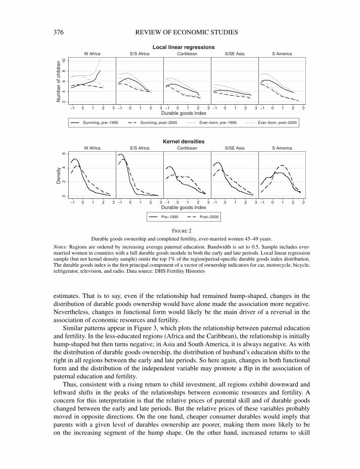
Figure 2 reveals pronounced variation in the relationship between durable goods ownershipand fertility, both across regions and within regions over time. In the least educated region, WestAfrica, both ever-born and surviving fertility monotonically increase in durable goods ownershipduring the early period, but the relationships flatten and even become slightly negatively-slopedin the late period. In most other regions, the relationships are initially hump-shaped but thenbecome everywhere negatively-sloped. One can interpret this disappearance of the hump-shapeas a shift in its peak towards resource levels lower than the sample minimum, so these resultsare consistent with a rising return to investment in children. The relationship’s changing shapecan alone flip the association of durable goods ownership with fertility, but such a flip would bebolstered by rising durable goods ownership in all regions, demonstrated by the kernel density
20. In the fertility history analyses, which pool multiple countries, the sampling weights are re-scaled to sum tonational populations in 1990 (for the pre-1995 sample) and 2010 (for the post-2005 sample).
[15:28 16/12/2015 rdv026_print.tex] RESTUD: The Review of Economic Studies Page: 376 365–401
376 REVIEW OF ECONOMIC STUDIES
24
68
10
−1 0 1 2 3 −1 0 1 2 3 −1 0 1 2 3 −1 0 1 2 3 −1 0 1 2 3
W Africa E/S Africa Caribbean S/SE Asia S America
Surviving, pre−1995 Surviving, post−2005 Ever−born, pre−1995 Ever−born, post−2005
Num
ber
of c
hild
ren
Durable goods index
Local linear regressions
0.2
.4.6
−1 0 1 2 3 −1 0 1 2 3 −1 0 1 2 3 −1 0 1 2 3 −1 0 1 2 3
W Africa E/S Africa Caribbean S/SE Asia S America
Pre−1995 Post−2005
Den
sity
Durable goods index
Kernel densities
Figure 2
Durable goods ownership and completed fertility, ever-married women 45–49 years.
Notes: Regions are ordered by increasing average paternal education. Bandwidth is set to 0.5. Sample includes ever-married women in countries with a full durable goods module in both the early and late periods. Local linear regressionsample (but not kernel density sample) omits the top 1% of the region/period-specific durable goods index distribution.The durable goods index is the first principal component of a vector of ownership indicators for car, motorcycle, bicycle,refrigerator, television, and radio. Data source: DHS Fertility Histories
estimates. That is to say, even if the relationship had remained hump-shaped, changes in thedistribution of durable goods ownership would have alone made the association more negative.Nevertheless, changes in functional form would likely be the main driver of a reversal in theassociation of economic resources and fertility.
Similar patterns appear in Figure 3, which plots the relationship between paternal educationand fertility. In the less-educated regions (Africa and the Caribbean), the relationship is initiallyhump-shaped but then turns negative; in Asia and South America, it is always negative. As withthe distribution of durable goods ownership, the distribution of husband’s education shifts to theright in all regions between the early and late periods. So here again, changes in both functionalform and the distribution of the independent variable may promote a flip in the association ofpaternal education and fertility.
Thus, consistent with a rising return to child investment, all regions exhibit downward andleftward shifts in the peaks of the relationships between economic resources and fertility. Aconcern for this interpretation is that the relative prices of parental skill and of durable goodschanged between the early and late periods. But the relative prices of these variables probablymoved in opposite directions. On the one hand, cheaper consumer durables would imply thatparents with a given level of durables ownership are poorer, making them more likely to beon the increasing segment of the hump shape. On the other hand, increased returns to skill

[15:28 16/12/2015 rdv026_print.tex] RESTUD: The Review of Economic Studies Page: 377 365–401
VOGL DIFFERENTIAL FERTILITY 377
24
68
0 5 10 15 20 0 5 10 15 20 0 5 10 15 20 0 5 10 15 20 0 5 10 15 20
W Africa E/S Africa Caribbean S/SE Asia S America
Surviving, pre−1995 Surviving, post−2005 Ever−born, pre−1995 Ever−born, post−2005
Num
ber
of c
hild
ren
Husband’s education
Local linear regressions
0.0
5.1
0 5 10 15 20 0 5 10 15 20 0 5 10 15 20 0 5 10 15 20 0 5 10 15 20
W Africa E/S Africa Caribbean S/SE Asia S America
Pre−1995 Post−2005
Den
sity
Husband’s education
Kernel densities
Figure 3
Paternal education and completed fertility, ever-married women 45–49 years.
Notes: Regions are ordered by increasing average paternal education. Bandwidth is set to 3. Sample includes ever-marriedwomen in countries with a full durable goods module in both the early and late periods. Local linear regression sample (butnot kernel density sample) omits the top 1% of the region/period-specific paternal education distribution. Data source:DHS Fertility Histories
would tend to move parents of a given skill level towards the declining segment of the humpshape. Both variables point to similar patterns, mitigating concerns about the confounding roleof prices.
In both figures, changing functional forms are evident for both ever-born fertility and survivingfertility. Which of these measures provides a better representation of the demand for childrendepends on the extent to which parents target surviving fertility. Given that fertility at ages 45–49years reflects sequential childbearing decisions and deaths over three decades, it seems reasonableto interpret surviving fertility as a closer proxy for the demand for children.21 Moreover, onlysurviving fertility is relevant for the composition effects estimated in Section 6; children who donot survive to adulthood do not affect the next generation’s skill distribution. For conciseness,the remaining analyses focus on counts of surviving children only.
To quantify these changes in functional form and assess their statistical significance,Tables 1–2 fit ordinary least squares (OLS) regressions of surviving fertility on the measuresof parental economic resources. The top panel of each table reports a linear specification tosummarize whether, on average, better-off parents exhibit higher or lower fertility. To address
21. Empirical research finds that parents “replace” deceased children rapidly (Ben-Porath, 1976), while theoreticalwork suggests that single-period models of the demand for children have similar quantitative implications to sequentialmodels with child mortality (Doepke, 2005).

[15:28 16/12/2015 rdv026_print.tex] RESTUD: The Review of Economic Studies Page: 378 365–401
378 REVIEW OF ECONOMIC STUDIES
TAB
LE
1D
urab
lego
ods
owne
rshi
pan
dsu
rviv
ing
fert
ilit
y,ev
er-m
arri
edw
omen
45–4
9ye
ars
W.A
fric
aE
./S.A
fric
aC
arib
bean
S./S
.E.A
sia
S.A
mer
ica
(Bur
kina
Faso
,Cam
eroo
n,(B
urun
di,K
enya
,(D
omin
ican
(Ind
ia,
(Col
ombi
a,G
hana
,Nig
er,
Mad
agas
car,
Mal
awi,
Nam
ibia
,R
epub
lic,
Indo
nesi
a)Pe
ru)
Nig
eria
,Sen
egal
)Ta
nzan
ia,Z
ambi
a,Z
imba
bwe
Hai
ti)
‘86–
’94
‘06–
’11
‘86–
’94
‘06–
’11
‘86–
’94
‘06–
’11
‘86–
’94
‘06–
’11
‘86–
’94
‘06–
’11
(1)
(2)
(3)
(4)
(5)
(6)
(7)
(8)
(9)
(10)
A.L
inea
rSp
ecifi
catio
nD
urab
lego
ods
inde
x0.
43−0.1
240.
004
−0.6
0−0.3
4−0.8
6−0.1
0−0.3
1−0.8
6−0.9
5[0.
15]∗
[0.04
6]∗[0.
102]
[0.07]∗
[0.10]∗
[0.06]∗
[0.03]∗
[0.02]∗
[0.10]∗
[0.04]∗
p-va
lue
for
diff
eren
ce0.
0004
<0.
0001
<0.
0001
<0.
0001
0.40
B.Q
uadr
atic
Spec
ifica
tion
Dur
able
good
sin
dex
0.46
−0.0
420.
01−0.5
4−0.2
0−1.0
1−0.0
37−0.3
2−0.7
9−1.3
5[0.
16]∗
[0.05
4][0.
09]
[0.07]∗
[0.11]
[0.07
7]∗[0.
034]
[0.03
0]∗[0.
15]∗
[0.06
8]∗Sq
uare
din
dex
−0.2
3−0.1
4−0.7
2−0.1
7−0.3
20.
23−0.1
80.
019
−0.0
870.
28[0.
11]∗
[0.04]∗
[0.09]∗
[0.06]∗
[0.10]∗
[0.05
0]∗[0.
026]∗
[0.01
8][0.
089]
[0.03
1]∗A
rgm
axof
quad
ratic
1.01
−0.1
50.
01−1.6
0−0.3
0—
−0.1
0—
−4.5
3—
[0.50]∗
[0.23]
[0.06]
[0.65]
[0.23]
[0.10]
[5.29]
p-va
lue
for
diff
eren
ce0.
035
0.01
3M
ean
inde
x−0.6
−0.1
−0.8
−0.5
−0.3
0.2
−0.4
0.0
0.4
0.8
Mea
nnu
m.o
fki
ds5.
05.
25.
95.
35.
04.
04.
13.
55.
33.
3O
bser
vatio
ns2,
772
8,24
72,
777
4,88
51,
132
3,11
211
,682
13,7
152,
356
8,00
2
Not
e:B
rack
ets
cont
ain
stan
dard
erro
rscl
uste
red
atth
epr
imar
ysa
mpl
ing
unit
leve
l.Sa
mpl
ein
clud
esev
er-m
arri
edw
omen
inco
untr
ies
with
afu
lldu
rabl
ego
ods
mod
ule
inbo
thth
eea
rly
and
late
peri
ods.
The
dura
ble
good
sin
dex
isth
efir
stpr
inci
palc
ompo
nent
ofa
vect
orof
owne
rshi
pin
dica
tors
for
car,
mot
orcy
cle,
bicy
cle,
refr
iger
ator
,tel
evis
ion,
and
radi
o.T
hear
gm
axis
the
ratio
ofth
elin
ear
term
toth
equ
adra
ticte
rm;i
tsst
anda
rder
ror
isco
mpu
ted
usin
gth
ede
ltam
etho
d.T
hesy
mbo
l“—
”in
dica
tes
aco
nvex
quad
ratic
func
tion,
whi
chha
sno
max
imum
.Dat
aso
urce
:DH
SFe
rtili
tyH
isto
ries
.*co
effic
ient
sign
ifica
ntat
the
5%le
vel.

[15:28 16/12/2015 rdv026_print.tex] RESTUD: The Review of Economic Studies Page: 379 365–401
VOGL DIFFERENTIAL FERTILITY 379
TAB
LE
2H
usba
nd’s
educ
atio
nan
dsu
rviv
ing
fert
ilit
y,ev
er-m
arri
edw
omen
45-4
9ye
ars
W.A
fric
aE
./S.A
fric
aC
arib
bean
S./S
.E.A
sia
S.A
mer
ica
(Bur
kina
Faso
,Cam
eroo
n,(B
urun
di,K
enya
,(D
omin
ican
(Ind
ia,
(Col
ombi
a,G
hana
,Nig
er,
Mad
agas
car,
Mal
awi,
Nam
ibia
,R
epub
lic,
Indo
nesi
a)Pe
ru)
Nig
eria
,Sen
egal
)Ta
nzan
ia,Z
ambi
a,Z
imba
bwe
Hai
ti)
‘86–
’94
‘06–
’11
‘86–
’94
‘06–
’11
‘86–
’94
‘06–
’11
‘86–
’94
‘06–
’11
‘86–
’94
‘06–
’11
(1)
(2)
(3)
(4)
(5)
(6)
(7)
(8)
(9)
(10)
A.L
inea
rSp
ecifi
catio
nH
usba
nd’s
educ
atio
n0.
087
−0.0
570.
036
−0.0
9−0.1
0−0.1
7−0.0
34−0.0
68−0.2
6−0.1
3[0.
026]∗
[0.00
7]∗[0.
019]
[0.01]∗
[0.02]∗
[0.01]∗
[0.00
6]∗[0.
005]∗
[0.02]∗
[0.01]∗
p-va
lue
for
diff
eren
ce<
0.00
01<
0.00
010.
001
<0.
0001
<0.
0001
B.Q
uadr
atic
Spec
ifica
tion
Hus
band
’sed
ucat
ion
0.29
0.08
0.19
0.01
0.12
0−0.3
40.
05−0.0
5−0.4
0−0.1
0[0.
08]∗
[0.02]∗
[0.04]∗
[0.03]
[0.06
3][0.
04]∗
[0.02]∗
[0.01]∗
[0.06]∗
[0.02
5]∗Sq
uare
ded
ucat
ion
−0.0
18−0.0
10−0.0
15−0.0
08−0.0
170.
012
−0.0
06−0.0
014
0.01
0−0.0
016
[0.00
6]∗[0.
002]∗
[0.00
3]∗[0.
002]∗
[0.00
4]∗[0.
002]∗
[0.00
1]∗[0.
0008]
[0.00
4]∗[0.
0013]
Arg
max
ofqu
adra
tic7.
943.
936.
080.
653.
53—
3.81
−17.
1—
−32.
6[0.
67]
[0.59]
[0.60]
[1.86]
[1.09]
[0.64]
[14.2]
[35.7]
p-va
lue
for
diff
eren
ce<
0.00
010.
005
0.14
Mea
nin
dex
−0.6
−0.1
−0.8
−0.5
−0.3
0.2
−0.4
0.0
0.4
0.8
Mea
nnu
m.o
fki
ds5.
05.
25.
95.
35.
04.
04.
13.
55.
33.
3O
bser
vatio
ns2,
772
8,24
72,
777
4,88
51,
132
3,11
211
,682
13,7
152,
356
8,00
2
Not
e:B
rack
ets
cont
ain
stan
dard
erro
rscl
uste
red
atth
epr
imar
ysa
mpl
ing
unit
leve
l.Sa
mpl
ein
clud
esev
er-m
arri
edw
omen
inco
untr
ies
with
afu
lldu
rabl
ego
ods
mod
ule
inbo
thth
eea
rly
and
late
peri
ods.
The
arg
max
isth
era
tioof
the
linea
rte
rmto
the
quad
ratic
term
;its
stan
dard
erro
ris
com
pute
dus
ing
the
delta
met
hod.
The
sym
bol
“—”
indi
cate
sa
conv
exqu
adra
ticfu
nctio
n,w
hich
has
nom
axim
um.D
ata
sour
ce:D
HS
Fert
ility
His
tori
es.*
coef
ficie
ntsi
gnifi
cant
atth
e5%
leve
l.

[15:28 16/12/2015 rdv026_print.tex] RESTUD: The Review of Economic Studies Page: 380 365–401
380 REVIEW OF ECONOMIC STUDIES
the theory of the hump-shaped relationship, the bottom panel reports quadratic models. If thecoefficient on the squared term is negative—consistent with a hump shape—then the bottompanel also provides the arg max of the quadratic function, estimated as the ratio of the linear termto the quadratic term.22 These estimates allow one to test whether the peak of the hump-shapehas shifted over time.
In the top panels of the tables, the linear association between parental resources and fertilitybecomes significantly more negative in four out of the five regions, irrespective of the measureof parental resources. The changes are starkest in Africa, where the association is initiallypositive. In West Africa, it flips from significantly positive to significantly negative, while inEastern and Southern Africa, it shifts from insignificantly positive to significantly negative.The other three regions exhibit negative associations in both periods. Supplementary AppendixTable 2 separates the sample into urban and rural areas, finding more positive coefficientsin rural areas; the coefficients go from positive to negative in rural parts of Western Africa,Eastern/Southern Africa, the Caribbean, and South/Southeast Asia. These results suggest a sharedprocess that visits urban areas before rural, first in Latin America, then in Asia, and finally inAfrica.
In the bottom panels of the tables, the quadratic specifications reveal significantly negativesquared term coefficients—indicating hump-shaped relationships—in the early period in four outof the five regions. In all four of these regions (and for both measures of economic resources),the arg max of the estimated function lands within the support of the distribution of economicresources. By the late period, however, the functional form changes dramatically. Either the argmax shifts significantly to the left or the relationship loses its hump-shape altogether, implyingan arg max that is infinitely negative. In some cases, the coefficient on the squared term eventurns significantly positive, which is consistent with the asymptotic properties of the skill-fertilityprofile in the theory. Here again, Latin America appears to have already arrived at the modernfertility regime in the early period.
These results may appear to contradict much existing research, which finds in the same datathat total fertility rates decrease with maternal education in most settings.23 The difference inresults has three likely sources. First, these other studies analyse total fertility rates, which mixthe fertility behaviour of older and younger cohorts; I focus on the completed fertility of theolder cohorts, thus capturing an earlier phase of the fertility transition. Second, the other sourcesonly look at all children ever born, while I consider counts of ever-born children and survivingchildren. The changing patterns are observable for both measures of fertility, but they are clearerfor counts of surviving children because child mortality is higher among the poor. Third, theother sources focus on maternal education, whereas I examine paternal education and durablegoods ownership, which bear a stronger link with income and the opportunity cost of time, due tolow rates of female labour force participation in many settings. For comparison with the existingliterature, Supplementary Appendix Table 3 includes the durables index, paternal education, andmaternal education in the same regression. Conditional on durable goods ownership and paternaleducation, maternal education is negatively associated with fertility in both periods.
4.2. Sibship size and educational attainment
The fertility history results provide evidence that the relationship between parental economicstatus and fertility was once hump-shaped, with a peak that shifted downward and leftward over
22. The standard error of the arg max estimate is computed using the delta method.23. See UN (1987, 1995), Cleland and Rodríguez, (1988) Mboup and Saha (1998), and Kremer and Chen (2002).

[15:28 16/12/2015 rdv026_print.tex] RESTUD: The Review of Economic Studies Page: 381 365–401
VOGL DIFFERENTIAL FERTILITY 381
time. But they do not give a sense of how pervasive these changes were historically—whetherthey occurred in Latin America, for example. Furthermore, they do not offer any information overthe implications of changing fertility differentials for average human capital. The sibling historiesoffer a window onto the issues for birth cohorts going back to the 1940s. Unfortunately, the DHScollects little data on economic conditions in childhood, but we can gain some insight into theevolution of the socioeconomic fertility differentials by studying changes in the relationshipbetween sibship size and education. The sibsize–education link is also directly relevant forassessing the effect of differential fertility on the skill distribution.
To capture the long-run evolution of this association, I estimate regressions separately bycountry and 5-year birth cohort (1945–1949 to 1985–1989).24 For woman i born in country c andcohort t, the regression specification is:
highestgradeict=δct+γctsibsizeict+εict, (4.1)
where highestgradeict denotes her schooling and sibsizeict denotes her sibship size.25
Focusing only on surviving sibship size for tractability, Figure 4 displays estimates of γct overtime within each country. Positive sibsize–education associations were pervasive until recentlybut have now largely disappeared. Specifically, for earlier birth cohorts, most coefficients aresignificantly positive, while for the latest birth cohorts, few coefficients are significantly positive,and many are significantly negative. Consistent with the fertility history results, this reversal inthe sibsize–education relationship occurs earliest in Latin America, followed soon thereafter byseveral countries in Asia. Africa’s reversal is quite recent; several countries remain in the pre-reversal regime. The Andean countries provide the starkest examples. For Bolivian women bornin the late 1940s, each additional sibling is associated with 0.4 more years of education, whereasfor those born in the 1980s, an additional sibling is associated with 0.5 fewer years of education.For Peruvian women, the associations swing from 0.2 to −0.6 over the same period.
Figure 4 reports findings for surviving sibship size because it bears a closer link to thecomposition effect and, arguably, the demand for children. But results for ever-born sibshipsize are similar. Supplementary Appendix Figure 1 plots the association between siblings everborn and completed education, again revealing coefficients that start broadly positive but becomenegative over time. The within-country, between-country, and overall correlations between theever-born coefficients and the surviving coefficients are all at least 0.95. Nevertheless, a possibleconcern for the interpretation of these results is that an adult respondent may not remember allof her deceased siblings, some of whom may have died before she was born.
4.3. Connecting the results
Results from the supplementary surveys in Bangladesh, Indonesia, and Mexico complement thesefindings in two ways. First, these surveys can address questions about gender heterogeneity, whichthe DHS cannot because it gathers sibling history data only from women. Since many countriesexhibit different patterns of investment in boys and girls, the exclusion of men leaves open thequestion of whether the association of family size with investment in boys changes in similar waysto the association of family size with investment in girls. The supplementary surveys interview
24. For precision, I omit cells with fewer than 200 observations, representing 2% of all cells.25. Researchers often control for birth order in estimating the effect of family size on educational attainment.
However, the present article is concerned not with causal effects but with equilibrium differences between large and smallfamilies, making regression adjustment unnecessary. Regardless, in unreported analyses, controlling for birth order didnot substantively affect the results.

[15:28 16/12/2015 rdv026_print.tex] RESTUD: The Review of Economic Studies Page: 382 365–401
382 REVIEW OF ECONOMIC STUDIES
−.5
0.5
1−
.50
.51
−.5
0.5
1−
.50
.51
−.5
0.5
1−
.50
.51
−.5
0.5
1−
.50
.51
−.5
0.5
1
1950 1960 1970 1980 19901950 1960 1970 1980 19901950 1960 1970 1980 19901950 1960 1970 1980 19901950 1960 1970 1980 1990
nineBhsedalgnaBnatsinahgfA
nooremaCaidobmaCidnuruBosaF anikruBaiviloB
erovI’D etoCognoC fo .peRCRDdahCcilbupeR nacirfA lartneC
aeniuGanahGnobaGaipoihtE.peR .moD
racsagadaMohtoseLaisenodnIayneKitiaH
aibimaNeuqibmazoMoccoroMilaMiwalaM
adnawRsenippilihPurePairegiNlapeN
naduSacirfA htuoSenoeL arreiSlageneSepicnirP & emoT oaS
ewbabmiZaibmaZogoTainaznaTdnalizawS
Coefficient
95% CI
5−year birth cohort
Figure 4
Association of surviving sibship size with education by period of birth.
Notes: From regressions of years of education on surviving sibship size. Sample includes all women over the age of 20years, except for the 2001 Bangladesh survey and the 1996 Nepal survey, which include ever-married women over theage of 30 years. Data source: DHS Sibling Histories

[15:28 16/12/2015 rdv026_print.tex] RESTUD: The Review of Economic Studies Page: 383 365–401
VOGL DIFFERENTIAL FERTILITY 383
both genders, allowing an investigation of this issue. In Supplementary Appendix Table 4, allthree supplementary surveys show declining sibsize–education relationships for both genders.Changes in the association of family size with child investment are not specific to girls.
Second, the supplementary surveys can help connect the fertility history results with the siblinghistory results. The fertility history results seem to contain the last phases of the global transitionto a negative relationship between parental economic status and fertility, while the sibling historyresults point to a widespread shift of the sibsize–education link from positive to negative. Whilethe two phenomena seem connected, the absence of childhood background characteristics foradult respondents in the DHS prevents examination of this issue. The supplementary surveys,however, include data on paternal education. Mirroring the DHS fertility history results, Figure 5shows a hump-shaped relationship between paternal education and surviving sibship size in allthree countries, with the peak shifting to the left over time. This shift even occurs in the middle-income context of Mexico, which had higher GDP per capita than all of the DHS countriesthroughout the sample period, suggesting that the DHS results are broadly representative of aphenomenon that spanned the developing world.26 Meanwhile, with extremely few exceptions,educational attainment monotonically rises in father’s education. In other words, higher-skillparents always educated their children more, but over time, they shifted from high to low relativefertility. Along these lines, Supplementary Appendix Table 5 shows that the evolution of thesibsize–education relationship has much to do with the changing relationship between paternaleducation and sibship size. Within each country, sibsize–education coefficients decrease acrosssuccessive birth cohorts, but controlling for paternal education mutes the reductions by half.
5. MECHANISMS OF THE REVERSAL
Viewed through the lens of the theoretical framework, the results so far are most consistent withan increase in the return to investment in children. The data point to flips in the overall associationsof economic status with fertility and of sibship size with education, both from positive to negative.Estimated non-parametrically, the relationship linking parental economic resources with fertilityis hump-shaped, with the peak moving downward and to the left over time. These patterns matchthe predictions of the theoretical framework under a goods cost of children and a rising returnto investment in children. However, the reversal of differential fertility occurred during a half-century of much economic and demographic change, offering a further testing ground for thishypothesis. This section further explores the mechanisms of the reversal, first by analysing theaggregate determinants of differential fertility and then by discussing how it relates to leadingalternative theories of demographic change.
5.1. Aggregate determinants of the reversal
This section estimates how changes in economic and demographic aggregates relate to changes inthe sibsize–education association, γct , which I treat as a summary statistic for differential fertility.I focus on the sibsize–education association rather than the resource–fertility association becausethe former offers a longer time horizon and is more precisely estimated at the country level. As inSection 4.2, I report results only for surviving sibship size, but unreported results for ever-bornsibship size coefficients are qualitatively similar.
26. The Mexico data also have counts of siblings ever born, which in unreported results also exhibit an initialhump shape.

[15:28 16/12/2015 rdv026_print.tex] RESTUD: The Review of Economic Studies Page: 384 365–401
384 REVIEW OF ECONOMIC STUDIES
01
23
45
6S
urvi
ving
sib
ship
siz
e
1940s 1950s 1960s 1970s
01
23
45
6S
urvi
ving
sib
ship
siz
e
1940s 1950s 1960s 1970s
01
23
45
6S
urvi
ving
sib
ship
siz
e
1940s 1950s 1960s 1970s
05
1015
Ow
n ye
ars
of e
duca
tion
1940s 1950s 1960s 1970s
05
1015
Ow
n ye
ars
of e
duca
tion
1940s 1950s 1960s 1970s
05
1015
Ow
n ye
ars
of e
duca
tion
1940s 1950s 1960s 1970s
None Primary Middle Secondary Post−secondary
Father’s education level
Indonesia Matlab, Bangladesh Mexico
Figure 5
Average sibship size and education by decade of birth and father’s education level, supplementary surveys.
Notes: Means are weighted by the survey weight divided by the surviving sibship size to make them representative ofthe families of surviving children. Data source: men and women born 1940–1979 in the Indonesia Family Life Survey(1993, 1997 waves), Matlab Health and Socioeconomic Survey (1996), and Mexico Family Life Survey (2002 wave)
5.1.1. Hypotheses. The rising-returns hypothesis makes several predictions regardingthe aggregate correlates of γct . First and second, a rise in the return to investment in childrenweakly decreases fertility and increases educational investment for all families. As a result,decreases in γct should be associated with declining average family size and rising average childinvestment. Third, in the presence of intergenerational human capital externalities, decreases inγct should be associated with rising average education among adults. As discussed in Section 2.3,such externalities would arise if more educated populations have more productive teachers.
The literature on the demographic transition cites several other forces as potentially importantin driving fertility change. One such force is income growth, which may reverse fertility gapsby pushing poor parents over the peak of the hump. This force fails to explain the changingform of the hump, but it also offers the testable implication that decreases in γct should beassociated with growth in living standards. A second force is the improving circumstance ofwomen. For example, rising female labour force participation may flip fertility differentials byincreasing the correlation between household income and the opportunity cost of childbearing.Alternatively, expansions in female education may alter bargaining power or norms in a way thatreverses fertility differentials. One can test these hypotheses with data on female labour forceparticipation and female educational attainment. Two final forces that arise often in discussionsof demographic change are mortality decline and urbanization, which one can examine directlyin the data.

[15:28 16/12/2015 rdv026_print.tex] RESTUD: The Review of Economic Studies Page: 385 365–401
VOGL DIFFERENTIAL FERTILITY 385
5.1.2. Method. I merge the panel of coefficients from Figure 4 with data on economicand demographic aggregates in the period of birth. Using the estimates of γct as the dependentvariable, I estimate:
γct=Z ′ctλ+τt+μc+εct, (5.1)
where Zct is a vector of economic and demographic aggregates, and τt and μc are cohortand country fixed effects, respectively. Residuals εct are clustered at the country level. Thespecification nets out global trends and time-invariant country characteristics, thus allowing oneto assess which aggregate changes are associated with the reversal of differential fertility. As abenchmark, one can measure the average magnitude of this reversal by leaving Zct out of equation(5.1). The resulting cohort effect estimates are flat through the early 1960s, at which point theybegin a downward trend, becoming significantly negative in the 1970s. Net of country fixedeffects, the sibsize–education association is on average 0.26 lower for the 1985–9 cohort than forthe 1945–9 cohort.
5.1.3. Results. The first set of estimations, appearing in Table 3, defines the covariatesZct as cohort average outcomes from the DHS: average completed education, average survivingsibship size, and the average fraction of siblings dying before they reach the age of 5 years.Because these average outcomes are co-determined with the sibsize–education relationship, oneshould think of the estimands as equilibrium associations rather than causal effects. For thisreason, I include only one covariate in each regression (in addition to the cohort and countryfixed effects). Also, because the estimates of γct and the cohort average outcomes are based onthe same data, the table supplements the OLS results with estimations that correct for correlatedmeasurement errors using Fuller’s (1987) method-of-moments technique. To ensure that thestandard errors fully capture variability from the first- and second-stage estimations, I bootstrapthe entire procedure, sampling within individual surveys before running the first stage and thensampling across countries before running the second stage. The OLS results and the Fullerresults give the same three conclusions: (1) as the sibsize–education association declines, averageeducational investment increases; (2) as the sibsize–education association declines, averagefamily size declines; and (3) the sibsize–education association has no relation to child mortalityrates. These findings support the rising-returns hypothesis while casting doubt on any role formortality decline or health improvement.
Table 4 regresses γct on three socioeconomic aggregates in the period of birth: log GDP percapita, average adult educational attainment, and urbanization. Data on these variables comefrom a variety of sources. GDP per capita is from from the Penn World Table (Heston et al.,2012); average adult (ages 25+ years) educational attainment is from Barro and Lee (2010) andCohen and Soto (2007); and urbanization is from UNDP (2011). To provide a summary measureof aggregate conditions at the time of fertility and child investment decisions, I average thesevariables over the 5-year period of birth.27 Since the education measure comes from two datasetsthat do not completely overlap, the table presents one regression for a combined sample and aseparate regression for each of the source samples. In the combined sample, I use the Barro–Leeestimates when available, and for countries that only have Cohen–Soto estimates, I use them to
27. GDP per capita is available annually, but the Barro–Lee education data and the UNDP urbanization data areavailable in 5-year increments, while the Cohen–Soto education data are available in 10-year increments. For these sources,I linearly interpolate across years before taking 5-year averages. Unreported results based on the closest measurementrather than interpolation are similar.

[15:28 16/12/2015 rdv026_print.tex] RESTUD: The Review of Economic Studies Page: 386 365–401
386 REVIEW OF ECONOMIC STUDIES
TABLE 3Demographic correlates of the sibship size-education relationship
Mean (SD) OLS Fuller OLS Fuller OLS Fuller(1) (2) (3) (4) (5) (6) (7)
Cohort average education 4.3 −0.045 −0.050(2.8) [0.019]∗ [0.023]∗
Cohort average surviving 4.4 0.100 0.106sibship size (0.7) [0.042]∗ [0.052]∗Cohort average fraction of 0.10 0.44 0.67siblings dying under 5 years (0.04) [0.79] [2.21]Number of observations 323 323 323 323 323 323 323Number of countries 43 43 43 43 43 43 43
Note: All analyses include birth cohort and country fixed effects. Fuller estimates correct for measurement error fromsampling variability. The dependent variable is the coefficient from a regression of education on surviving sibship size.Brackets contain bootstrapped standard errors. The bootstrap procedure resamples respondents from each survey beforeestimating country-cohort parameters and then resamples entire countries before estimating the analyses reported in thetable Data source: DHS Sibling Histories. *coefficient significant at the 5% level.
TABLE 4Development and the sibship size–education relationship
OLS OLS OLS(1) (2) (3)
Ln(GDP per capita in birth period) 0.030 0.014 0.065[0.074] [0.076] [0.069]
Avg. adult yrs. ed. in birth period −0.101 −0.113 −0.128[0.027]∗ [0.031]∗ [0.028]∗
Fraction urban in birth period −0.33 −0.27 −0.10[0.45] [0.47] [0.36]
Number of observations 227 203 162Number of countries 39 35 30Education dataset Combined Barro–Lee Cohen–Soto
Note: All regressions include birth cohort and country fixed effects. The dependent variable is the coefficient from aregression of education on surviving sibship size. Brackets contain standard errors clustered at the country level. The“combined” measure uses the Barro–Lee data if available and otherwise projects the Cohen–Soto data onto the Barro–Leescale. *coefficient significant at the 5% level.
generate predicted Barro–Lee estimates based on a regression of Barro–Lee on Cohen–Soto. Allthree regressions lead to the same conclusion: while aggregate income growth and urbanization donot play a role, the rising educational attainment of the parent generation is intimately connectedwith the reversal of the sibsize–education relationship among offspring. In fact, the coefficientof −0.09 on average education implies that rising education can account for roughly 60% of theof 1985–9 cohort effect for γct , as reported at the start of this section. Again, these findings bestmatch the rising-returns hypothesis, while discrediting theories centered on income growth andurbanization.
Several alternative theories deal with the position of women; these theories are the subjectof Table 5. Data on the variables in Table 5 are only available for small subsamples, so tomaximize sample size, each regression uses a different sample. The table first addresses theoriesinvolving the expansion of women’s labour market opportunities. Goldin (1995) argues thatwomen’s work becomes incompatible with child rearing only when it moves outside the home,such that agricultural work is less likely to compete with parenting than service work. If women’sopportunity cost of time explains the reversal, then the emergence of the service sector must

[15:28 16/12/2015 rdv026_print.tex] RESTUD: The Review of Economic Studies Page: 387 365–401
VOGL DIFFERENTIAL FERTILITY 387
TABLE 5Female empowerment and the sibship size–education relationship
OLS OLS OLS(1) (2) (3)
Women’s labour force participation rate in birth period 0.045[0.101]
Manufacturing fraction of value added in birth period 0.06[0.21]
Services fraction of value added in birth period −0.02[0.23]
Avg. adult male yrs. ed. in birth period −0.071[0.021]∗
Avg. adult female yrs. ed. in birth period −0.051[0.033]
p-value: joint test of education coefficients 0.002p-value: difference of education coefficients 0.851Number of observations 115 144 246Number of countries 35 41 35
Note: All regressions include birth cohort and country fixed effects. The dependent variable is the coefficient from aregression of education on surviving sibship size. Brackets contain standard errors clustered at the country level. Theeducation measures in column (3) are from the Barro–Lee dataset. *coefficient significant at the 5% level.
also play a key role. To explore the role of the opportunity cost of women’s time, Columns (1)and (2) thus regress γct on the women’s (ages 20–59 years) labour force participation rate (fromILO 2012 and Olivetti, 2014) and the sectoral composition of value added (from Heston et al.,2012).28 Neither variable plays a role in the reversal of the sibsize–education association. Anothergender-specific theory emphasizes female education over male. Column (3) thus uses gender-disaggregated education data, available only from the Barro–Lee dataset, to ask whether therole of average education is due to women or men. While the coefficients on average femaleeducation and average male education are jointly significantly different from zero, they are notsignificantly different from each other; in fact, the coefficient on average male education is largerand individually more significant. Table 5 suggests that the causes of the reversal are not specificto the empowerment of women.
5.2. Relation to other theories of demographic change
Combined with the non-monotonic patterns in Section 4, the aggregate panel results favour thehypothesis that rising returns to investment in children reversed fertility differentials by incomeand skill. Income growth, urbanization, mortality decline, and women’s empowerment appear tohave played little role in the reversal. However, the literature on the demographic transition—especially in disciplines outside economics—suggests some alternative theories of the reversalthat the results so far do not directly address.
In interpreting the changing cross-sectional patterns, many non-economists would think firstof preferences, rather than prices or returns. Several theories of fertility decline (Caldwell, 1980,1982; Casterline, 2001) posit changes in beliefs and norms regarding child-rearing, and someversions of these theories could explain the observed regime change. Consider the introductionof new “Western” norms that increase the relative importance of child quality in the utility function
28. Sectoral composition is available on an annual basis, but female labour force participation is measuredsporadically, so I linearly interpolate country values between measurements. Unreported analyses using only un-interpolated values led to the same conclusions.

[15:28 16/12/2015 rdv026_print.tex] RESTUD: The Review of Economic Studies Page: 388 365–401
388 REVIEW OF ECONOMIC STUDIES
(β), raising optimal education and lowering optimal fertility. If these norms affect the richest (ormost educated) families most strongly, then the relationship between fertility and income (or skill)could flip from positive to negative, starting at the right tail of the income distribution. Caldwell,1980, 1982) assigns much importance to mass education in altering childbearing norms, thuspredicting a relationship between γct and average adult educational attainment. Without furtherstructure, the theory is otherwise difficult to test. But if one views the norms as increasing thesocial return to education spending (θ1), then the norms theory coincides with the rising-returnshypothesis.
An alternative version of the norms theory associates the diffusion of new norms with theempowerment of women. If women have higher β’s than men, and if women of higher income oreducation make the earliest gains in household bargaining power, then richer households will bethe first to transition to low fertility. Unlike the broader norms theory, one can reject the role offemale empowerment on the basis of the results in Table 5. Neither women’s work nor women’sschooling plays an important role in the reversal of differential fertility.
A separate class of theories emphasizes upward intergenerational transfers from children toparents, in the form of child labour or old-age support.29 In the theoretical framework of Section2, the falling prevalence of child labour has similar consequences to a rising return to childinvestment. Some of the decline in child labour may actually be the result of increases in thereturn to child investment. Some might also be due to new sanctions against child labour, whichone could characterize as increases in the goods cost of children κ . Just as with an increase in thereturn to child investment, an increase in the goods cost of children decreases the wage thresholdat which families start to spend on education, which can shift the peak of the fertility hump to theleft. This mechanism is complementary to the return-to-investment hypothesis.
Other theories stressing intergenerational transfers do not fit as well into Section 2’sframework. Under an old-age security motive for childbearing, for example, financial deepeningcould flip the income–fertility relationship if wealthy families substituted other savings vehiclesfor children. But this reasoning gives no account for why decreases in quantity investment wouldbe accompanied by increases in quality investment. Furthermore, as stressed by Galor (2011),wealthier couples typically have access to a wider variety of savings vehicles before the fertilitytransition. Finally, Lee (2000) argues no society exhibits a net upward flow of resources acrossgenerations, unless one counts the pension systems of rich countries. Based on these insights, theold-age support motive is unlikely to explain the reversal of differential fertility.
Nevertheless, some specific institutional arrangements do give rise to significant pecuniaryreturns to having many adult offspring. For example, Tertilt (2005) posits that men in polygynoussocieties have an incentive to invest their wealth in a large number of children. In such societies,a groom typically “buys” a bride from her father, so men benefit from having many daughtersbut do not lose from having many sons. Consistent with this idea, the average sibsize–educationassociation in polygynous countries exceeds that in monogamous countries by 0.1 to 0.2, bothwithin Africa and across the world.30 But declining polygyny cannot explain the global patternsdocumented in Section 4 because both polygyny and bride price were rare in many samplecountries throughout the study period.
Instead of the prices or returns associated with childbearing, advocates of family planningmight emphasize the uneven adoption of effective contraceptive technology (Potts, 1997). Fromthis perspective, the currently negative relationship between income and fertility is due to anunmet need for contraception among the poor. But a theory of this type fails to account for the
29. See Cain (1983), Nugent (1985), Ehrlich and Lui (1991), Morand (1999), and Boldrin and Jones (2002).30. Note that the patterns here must be driven by the number of children per wife, not the number of wives per
husband. The DHS sibling history asks for siblings with the same biological mother.
[15:28 16/12/2015 rdv026_print.tex] RESTUD: The Review of Economic Studies Page: 389 365–401
VOGL DIFFERENTIAL FERTILITY 389
early regime during which fertility increases in income. One possibility is that women fromricher households have a higher biological capacity to bear children due to their better health.But this theory receives little support from the data, which show little relation between healthimprovements (as measured by child mortality rates) and the reversal of differential fertility.Theories that involve changes in the demand for children appear to provide a better fit to the data.
6. DIFFERENTIAL FERTILITY AND AVERAGE EDUCATION
The results so far suggest that differential fertility once promoted aggregate human capitalaccumulation rather than hindering it. This section delves into the magnitudes of these effects.Recall that equation (2.7) separated the effect of differential fertility on average human capitalinto two components: a composition effect, reflecting how fertility heterogeneity reshapes thepopulation in the next generation, and an adjustment effect, reflecting how the change fromexogenous to endogenous fertility alters parental optimization. To give a quantitative sense ofboth composition and adjustment effects on child investment, it first calibrates the model fromSection 2 using an Indonesian dataset from the 1970s. It then returns to the DHS data, presentingnon-parametric estimates of the composition effect on average education.
6.1. Model calibration of composition and adjustment effects
Because the datasets used in Sections 4–5 do not offer information on parental wages, I draw onyet another, the 1976 Indonesia Intercensal Population Survey (SUPAS), for model calibration.SUPAS is one of few developing-country datasets of its era with a large sample and informationon labour income and hours worked. I calibrate the model to match patterns of surviving fertilityamong married women aged 45–54 year with husbands in wage- or salary-paying jobs. Becausemany of the respondents to the Indonesia Family Life Survey were born to this cohort of women,one can view these fertility patterns as mapping roughly onto the supplementary survey resultsin Figure 5. I separate husbands into five skill categories (none, incomplete primary, completeprimary, complete middle, complete secondary and above) and define full annual income as theaverage hourly wage in each skill category times 16 hours per day times 365 days. Full annualincome rises with skill and averages $5,104, measured in PPP-adjusted 2011 international dollars.
To parametrize the model, I first set the time cost τ , followed by the preference parameters αandβ, the goods cost κ , and finally the parameters of the human capital production function θ0 andθ1. I assume no subsistence constraint. In choosing τ , I follow De la Croix and Doepke (2003),who set it at 0.075 based on evidence from Haveman and Wolfe (1995) and Knowles (1999) thata child costs her parents 7.5% of their adult time endowment. I calibrate the preference parameterα to minimize the distance between each skill group’s optimal fertility in the model and itsaverage number of surviving children in the data, with equal weight given to each skill group.Given the parameter choices below, this approach leads to α=0.438, implying that parents spend44% of their full income on their consumption. One can then back out β with an assumptionregarding the limit of optimal fertility n∗H as H approaches infinity. I assume that asymptotic
fertility n∗∞= (1−α)(1−β)τ equals 2, which implies β=0.733.31
One can additionally use α to set an appropriate goods cost of children. Using data fromIndonesia during the same period, Muellbauer and Deaton (1986) apply equivalence scale methods
31. The assumption that fertility approaches 2 as H approaches infinity may appear to be at odds with currentfertility patterns in Europe and East Asia, where total fertility rates are lower than 2. However, for the relatively poorpopulations under consideration, the assumption that fertility approaches replacement levels seems reasonable.

[15:28 16/12/2015 rdv026_print.tex] RESTUD: The Review of Economic Studies Page: 390 365–401
390 REVIEW OF ECONOMIC STUDIES
Optimal fertility, model
Average number of surviving children, 1976 data
Population share, 1976 data
010
2030
40P
erce
nt o
f pop
ulat
ion
3.5
44.
55
5.5
6N
umbe
r of
chi
ldre
n
0 5000 10000 15000 20000 25000Average annual full income in skill level, PPP (2011 international dollars)
Figure 6
Model calibration, Indonesia.
Notes: Sample includes 1246 married women aged 45–54 years with husbands in wage- or salary-paying jobs. Each pointrepresents a skill group based on the husband’s education: from left to right, none, incomplete primary, complete primary,complete middle, and complete secondary and above. Data source: SUPAS 1976
to conclude that a child costs 30–40% of an adult. I choose the midpoint of this range and followDe la Croix and Doepke (2003) in supposing that parents live with their children for half of theiradult lives. Assuming that the equivalence scale estimate holds for parents at the median fullincome level, and that parents at this full income level do not invest in their children, I thus setκ to be 0.175 times α times median full income, or $217 per year of adulthood. This value landsbetween the child costs implied by Indonesia’s urban and rural per capita poverty lines for 1976.
Finally, the values of θ0 and θ1 only affect the solution through the ratio θ0θ1
, which one canobtain by combining the preceding parameter choices with an assumption regarding the peak ofthe n∗H curve. Among the five skill groups in the data, the highest average number of survivingchildren is 5.8, but because the n∗H curve reaches its maximum between two skill levels, I assume a
peak fertility level of 6.5 to add flexibility to the model.32 This assumption implies that θ0θ1=1198.
This parametrization predicts an average fertility rate of 4.78, relative to 4.82 in the data.Figure 6 displays each skill group’s population share and average fertility in the data, as wellas the model’s predictions. As in Figure 5’s results for Indonesia, fertility is lowest among thelowest-skill parents, who comprise the largest share of the population. It is highest at intermediateskill levels. Relative to the data, the model slightly understates fertility at low skill levels, slightlyoverstates fertility at intermediate skill levels, and matches fertility among the highest-skilledparents. Starting from this baseline parametrization, Table 6 presents a series of computationalexperiments.
32. Assuming lower peak fertility does not alter model’s predictions regarding differential fertility and its effects,but it leads the model to understate mean fertility.

[15:28 16/12/2015 rdv026_print.tex] RESTUD: The Review of Economic Studies Page: 391 365–401
VOGL DIFFERENTIAL FERTILITY 391
TABLE 6Computational experiments, Indonesia
Education Effect of differential fertility on education spendingspending per child [Expressed as a share of column (2)]
Average per as share of Compositionfertility (n) child tot. spending effect
Adjustment effects
ñ = nmin ñ = n ñ = nmax
(1) (2) (3) (4) (5) (6) (7)
Baseline 4.78 $38 3% 18% −216% −28% 48%Effect of 10% rise in…θ1 only 4.63 $57 5% 5% −128% 0% 67%w only 4.78 $59 5% 4% −110% 4% 68%Both θ1 and w 4.67 $74 6% −9% −76% 20% 73%Effect of 20% rise in…θ1 only 4.54 $70 6% −6% −97% 15% 73%w only 4.80 $75 5% −9% −64% 22% 82%Both θ1 and w 4.66 $95 7% −31% −105% 43% 73%
Note: Parameter choices described in text. Education spending per child is denominated in PPP-adjusted 2011 internationaldollars and reflects average annual spending over parents’ adult lives. Sample includes 1246 married women aged 45–54years with husbands in wage- or salary-paying jobs. Data source: SUPAS 1976.
The first row of Table 6 further summarizes the baseline parametrization.As shown in columns(2)–(3), education spending amounts to $38 per child, or 3% of total expenditure. The remainingcolumns of the table report the effect of differential fertility on education spending per child,expressed as a share of the quantity in column (2). I focus on education spending rather thanhuman capital because it is the closest analogue to educational attainment, which we observe inthe data. Column (4) reports the composition effect, which raises education spending per childby 18% of the $38 reported in column (2).
In columns (5)–(7), the focus shifts to adjustment effects for different values of exogenousfertility n, which vary widely. Compared to a counterfactual in which fertility is exogenously setat the lowest observed fertility level, endogenous fertility reduces parents’ average educationalinvestments per child by over 200% of the $38 reported in column (2). Since the lowest-skillparents exhibit the lowest fertility, the low exogenous fertility level forces all other parents tohave fewer children, so that educational investment is substantially higher in the counterfactual. Incontrast, when the counterfactual sets fertility at its maximum observed level, the adjustment effectbecomes positive, at 48%. When fertility is exogenously set at its average in the counterfactual,the effect shrinks to −28%.
The remaining rows of Table 6 consider how 10–20% increases in investment returns andwages affect average fertility, average education spending, and the effects of differential fertility.As predicted in Section 2, an increase in θ1 alone reduces average fertility, raises average educationspending, and reduces the composition effect of differential fertility, which eventually turnsnegative. While an increase in w alone has similar effects on average education spending andthe composition effect, it also raises average fertility because most families are on the increasingsegment of the fertility profile. Because the aggregate panel results suggest that fertility declinetypically accompanies the flip of the association between fertility and child investment, the databetter fit a rise in θ1. However, the calibration results also show that simultaneous increases in θ1and w also reduce average fertility, raise average education spending, and reduce the compositioneffect. Throughout all of these computational experiments, the adjustment effect continues tovary wildly with the exogenous fertility level.

[15:28 16/12/2015 rdv026_print.tex] RESTUD: The Review of Economic Studies Page: 392 365–401
392 REVIEW OF ECONOMIC STUDIES
Although the article has focused on a single, exogenous fertility level as its main thoughtexperiment, other counterfactuals are also of interest. For example, De la Croix and Doepke(2003) argue that when fertility monotonically declines with skill, higher inequality reduceseducation spending per child.33 But this conclusion can change dramatically with a hump-shaped relationship between fertility and skill. Holding fixed the mean of the full incomedistribution, a 10% increase in its standard deviation raises education spending per childby roughly one-half, to $58, in the baseline parametrization. Conversely, a mean-preserving,10% decrease in spread reduces education spending per child by more than one-half,to $16.
Although changes in variance are informative, some may be more interested in the effectsof implementable policies. A 10% tax on labour income that is redistributed in the form ofa lump-sum transfer reduces education spending per child by even more, to $8. Compared tothe mean-preserving reduction in spread, this redistributive policy has stronger negative effectsbecause it reduces the opportunity cost of time and raises non-labour income, both of whichraise fertility and decrease child investment. If the tax revenue is returned in the form of achild tax credit, the investment disincentive becomes so strong that no parents invest in theirchildren. Another policy instrument of interest is a one-child policy, which dramatically limitsparents’ choice sets, reducing fertility by 60–83%. Such a policy would bind far more thanChina’s famous law, which affected only a portion of the population and was implemented afterfertility had already declined by half over the preceding decade, to three children per woman(Hesketh et al., 2005). In any case, this sharp contraction in fertility leads to a 41-fold increasein education spending per child, primarily reflecting re-optimization rather than compositionalchanges. Importantly, these quantities and the adjustment effects in Table 6 ignore any generalequlibrium effects.
6.2. Non-parametric estimates of the composition effect
Composition effects in the calibrated model begin at 18% of education spending per child anddecline to mildly negative values with moderate increases in θ1 or w. Because the compositioneffect is a function of the realized joint distribution of fertility and child investment, one can verifythese magnitudes in the data. Equation (2.7) expressed the composition effect by integrating overthe parental wage distribution. I only observe siblings, with little information about their parents,so the formula for the composition effect is not directly estimable. Applying the law of iteratedexpectations, however, one can rewrite it over the distribution of surviving sibship sizes:
�comp(F)=K∑
k=1
(ηk− ηk/k∑K
l=1ηl/l
)μk, (6.1)
where K is the maximum possible sibship size, ηk is the share of the individuals from survivingsibships of size k, and μk is the mean human capital (or educational investment) of individualsfrom sibships of size k. Inside the parentheses, the term ηk weights the sample to give meanhuman capital across individuals, while the term ηk/k∑K
l=1ηl/lreweights the sample to give mean
human capital (or educational investment) across families. Attractively, this expression capturesany composition effect of heterogeneity in fertility and skill investment, not just the heterogeneity
33. De la Croix and Doepke find that higher inequality reduces the next generation’s human capital, which resultsfrom both the concavity of their human capital production function and changes in education spending per child.

[15:28 16/12/2015 rdv026_print.tex] RESTUD: The Review of Economic Studies Page: 393 365–401
VOGL DIFFERENTIAL FERTILITY 393
specific to the model in Section 2. Nevertheless, the reweighted mean omits childless couples.This omission is not an issue in the context of the model, in which no couples choose to bechildless. But in practice, the counterfactual average represents a world in which the offspring ofactual parents, rather than potential parents, are equally represented in the next generation. I usethe empirical analogues of ηk and μk to estimate �comp and obtain its variance using the deltamethod.
I begin with estimates of the composition effect on average educational investment, whichbears the closest link to the calibration results in Section 6.1. For successive 5-year birth cohortswithin each country, Figure 7 displays estimates of the composition effect of differential fertilityon mean educational attainment. The results overturn the conventional wisdom that variation infertility over the skill or income distribution tends to lower mean education. Only South Africaexhibits a significantly negative composition effect for the earliest cohort. In some countries,predominantly African, differential fertility increased mean educational attainment throughoutthe sample period. Most of the remaining countries have undergone a transition from a regimein which differential fertility promoted the growth of mean education to a regime in whichdifferential fertility depressed it. For two compelling examples, consider the Andean nations ofBolivia and Peru. In the 1945–9 cohort, differential fertility increased mean education by 0.3 to0.5 years in both countries; in the 1985–9 cohort, differential fertility reduced average educationby 0.5 years.
One can shed light on the importance of these magnitudes by expressing each cohort’scomposition effect as a share of its mean educational attainment. Figure 8 carries out this exercise,with the composition effect as a share of mean education on the vertical axis and mean educationon the horizontal axis. A local linear regression (with a bandwidth of 1 year) captures how therelative importance of the composition effect changes with rising mean education. At low levelsof mean education, the composition effect is proportionally large and positive, raising meaneducation by as much as one-third and by 15% on average. This result bears striking similarityto the baseline calibration result in Indonesia. As mean education increases, the compositioneffect trends downward, becoming negative when mean education reaches the secondary level.Proportionally, these negative composition effects are small, averaging 5% of mean education.Contrary to the assumptions of much of the literature on differential fertility and economic growth,composition effects are positive when they are proportionally most important. The 15% positiveeffect may or may not be large enough to play an important role in endogenous growth, but it ismore likely to do so than the 5% negative effect.
Another way to place these composition effects in context is to calculate the extent to whichdifferential fertility affects cross-country skill gaps. Data are available for all sample countriesfor the birth cohorts of the 1960s and early 1970s. According to Barro and Lee (2010), the USleads the world in average female education for these cohorts. To study the effects of differentialfertility at the frontier of female human capital, I thus use data from the National LongitudinalSurvey of Youth 1979 (NLSY79), which covers US birth cohorts from 1958 to 1965. Amongwomen in the NLSY79, the composition effect is −0.17 years of education, amounting to1.3% of mean educational attainment. The NLSY79 thus suggests that the composition effectremains proportionally small even at mean education levels higher than those observed in DHScohorts.
Table 7 combines the NLSY79 and the DHS to ask how differential fertility affects eachDHS country’s distance to the human capital frontier for women of the 1958–65 birth cohort. Forreference, columns (1) and (2) report actual and reweighted mean educational attainment; thedifference between the two is the composition effect. In this early birth cohort, the compositioneffect is positive for most countries. Columns (3)–(5) then estimate how much larger or smaller isa country’s distance to the human capital frontier as a result of differential fertility, compared to
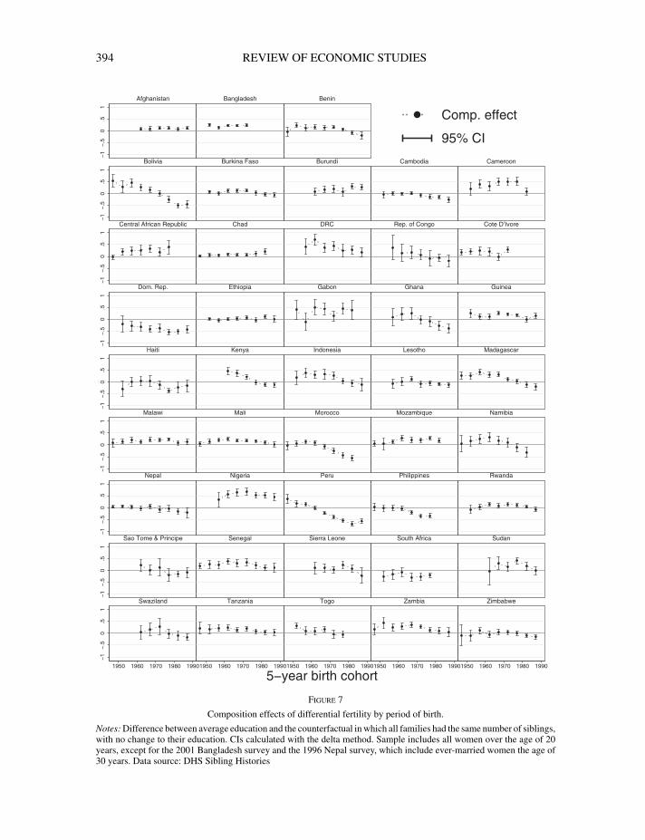
[15:28 16/12/2015 rdv026_print.tex] RESTUD: The Review of Economic Studies Page: 394 365–401
394 REVIEW OF ECONOMIC STUDIES
−1
−.5
0.5
1−
1−
.50
.51
−1
−.5
0.5
1−
1−
.50
.51
−1
−.5
0.5
1−
1−
.50
.51
−1
−.5
0.5
1−
1−
.50
.51
−1
−.5
0.5
1
1950 1960 1970 1980 19901950 1960 1970 1980 19901950 1960 1970 1980 19901950 1960 1970 1980 19901950 1960 1970 1980 1990
Afghanistan Bangladesh Benin
Bolivia Burkina Faso Burundi Cambodia Cameroon
erovI’D etoCognoC fo .peRCRDdahCcilbupeR nacirfA lartneC
aeniuGanahGnobaGaipoihtE.peR .moD
racsagadaMohtoseLaisenodnIayneKitiaH
aibimaNeuqibmazoMoccoroMilaMiwalaM
adnawRsenippilihPurePairegiNlapeN
Sao Tome & Principe Senegal Sierra Leone South Africa Sudan
ewbabmiZaibmaZogoTainaznaTdnalizawS
Comp. effect
95% CI
5−year birth cohort
Figure 7
Composition effects of differential fertility by period of birth.
Notes: Difference between average education and the counterfactual in which all families had the same number of siblings,with no change to their education. CIs calculated with the delta method. Sample includes all women over the age of 20years, except for the 2001 Bangladesh survey and the 1996 Nepal survey, which include ever-married women the age of30 years. Data source: DHS Sibling Histories

[15:28 16/12/2015 rdv026_print.tex] RESTUD: The Review of Economic Studies Page: 395 365–401
VOGL DIFFERENTIAL FERTILITY 395
TAB
LE
7D
iffer
enti
alfe
rtil
ity
and
dist
ance
toth
ehu
man
capi
talf
ront
ier,
wom
enbo
rn19
58–1
965
Com
p.ef
fect
ofdi
ff.f
ert.
Com
p.ef
fect
ofdi
ff.f
ert.
Rew
t.on
dist
ance
tofr
ontie
rin
…R
ewt.
ondi
stan
ceto
fron
tier
in…
Avg
.ed.
avg.
ed.
Avg
.ed.
Avg
.HC
Agg
.HC
Avg
.ed.
avg.
ed.
Avg
.ed.
Avg
.HC
Agg
.HC
(1)
(2)
(3)
(4)
(5)
(1)
(2)
(3)
(4)
(5)
Afg
hani
stan
0.43
0.36
−1.8
%−2.3
%−2.1
%N
iger
ia3.
953.
65−4.6
%−5.1
%−5.3
%N
epal
0.66
0.65
−1.4
%−1.9
%−1.9
%D
RC
4.04
3.69
−5.0
%−5.4
%−5.7
%B
urki
na0.
670.
54−2.2
%−2.7
%−2.5
%M
adag
asca
r4.
043.
70−5.0
%−5.3
%−5.7
%E
thio
pia
0.67
0.67
−1.2
%−1.8
%−1.8
%S.
Tom
e&
Prin
cipe
4.06
3.89
−3.4
%−3.8
%−4.0
%C
had
0.72
0.65
−1.8
%−2.3
%−2.2
%Ta
nzan
ia4.
123.
83−4.6
%−4.9
%−5.1
%M
ali
1.04
0.80
−3.1
%−3.5
%−3.2
%C
amer
oon
4.39
3.99
−5.7
%−6.0
%−5.7
%B
urun
di1.
051.
02−1.5
%−2.1
%−2.0
%G
hana
5.18
4.86
−5.4
%−5.7
%−5.6
%G
uine
a1.
090.
94−2.4
%−2.9
%−2.7
%Z
imba
bwe
5.61
5.61
−2.1
%−2.6
%−2.8
%B
enin
1.48
1.36
−2.3
%−2.8
%−2.7
%Z
ambi
a5.
625.
30−5.8
%−6.1
%−6.1
%Su
dan
1.56
1.03
−5.4
%−5.8
%−5.0
%K
enya
6.04
5.61
−7.3
%−7.5
%−7.7
%M
ozam
biqu
e1.
651.
53−2.3
%−2.8
%−2.7
%In
done
sia
6.23
5.88
−6.5
%−7.0
%−7.1
%Se
nega
l1.
821.
44−4.4
%−4.7
%−4.3
%B
oliv
ia6.
296.
17−3.8
%−4.2
%−4.5
%Si
erra
Leo
ne1.
911.
68−3.2
%−3.7
%−3.4
%N
amib
ia6.
346.
30−2.7
%−3.3
%−3.4
%C
entr
alA
fric
anR
ep.
2.08
1.82
−3.6
%−3.9
%−3.7
%Sw
azila
nd6.
396.
580.
2%−0.8
%−0.6
%C
ote
D’I
vore
2.10
1.97
−2.5
%−3.0
%−2.9
%G
abon
6.66
6.27
−7.3
%−7.9
%−8.1
%B
angl
ades
h2.
151.
97−3.0
%−3.4
%−3.3
%R
ep.O
fC
ongo
6.66
6.17
−8.5
%−8.8
%−9.3
%To
go2.
252.
24−1.6
%− 2.1
%−2.1
%L
esot
ho6.
776.
83−1.6
%−2.5
%−2.4
%H
aiti
2.43
2.30
−2.6
%−3.0
%−3.0
%D
omin
ican
Rep
.7.
618.
044.
4%3.
7%4.
3%C
ambo
dia
2.44
2.43
−1.5
%−2.1
%−2.1
%So
uth
Afr
ica
7.94
8.19
1.4%
0.4%
−0.1
%M
oroc
co2.
442.
35−2.3
%−2.8
%−2.7
%Pe
ru8.
058.
11−1.9
%−2.5
%−3.2
%R
wan
da2.
622.
59−1.7
%−2.3
%−2.3
%Ph
ilipp
ines
8.90
8.94
−2.5
%−3.3
%−3.8
%M
alaw
i2.
882.
73−2.9
%−3.4
%−3.4
%A
vera
ge3.
743.
60–3
.1%
–3.6
%–3
.6%
Not
e:C
ount
ries
orde
red
byav
erag
eed
ucat
ion.
The
Bar
ro–L
eeda
tase
tin
dica
tes
that
the
US
isth
efe
mal
ehu
man
capi
tal
fron
tier.
Ius
eth
eN
LSY
79(1
958–
1965
coho
rt)
toco
mpu
teav
erag
efe
mal
eed
ucat
ion
(13.
75ye
ars)
and
rew
eigh
ted
aver
age
educ
atio
n(1
3.92
year
s)at
the
fron
tier.
Toco
mpu
te“a
vera
gehu
man
capi
tal”
,Itr
ansf
orm
year
sof
educ
atio
nto
Hal
land
Jone
s’sh
uman
capi
talm
easu
rean
dth
enav
erag
eac
ross
indi
vidu
als.
Toco
mpu
te“a
ggre
gate
hum
anca
pita
l”,I
aver
age
year
sofe
duca
tion
and
then
perf
orm
the
Hal
land
Jone
stra
nsfo
rmat
ion.

[15:28 16/12/2015 rdv026_print.tex] RESTUD: The Review of Economic Studies Page: 396 365–401
396 REVIEW OF ECONOMIC STUDIES
−.2
−.1
0.1
.2.3
.4(C
ompo
sitio
n ef
fect
)/(A
vera
ge)
0 2 4 6 8 10Cohort average education
Figure 8
Composition effects as a share of average education.
Notes: The curve is a local linear regression with a bandwidth of 1 year. The composition effect is the difference betweenaverage education and the counterfactual that would arise if all families had the same number of siblings, with no changeto their education. Sample includes all women over the age of 20 years, except for the 2001 Bangladesh survey and the1996 Nepal survey, which include ever-married women over the age of 30 years. Data source: DHS Sibling Histories
a counterfactual in which both the DHS and the US data are reweighted to remove the compositioneffect of differential fertility. This effect is expressed proportionally:
Effect on distance to the frontier= hUS−hc(hUS−�comp,US
)−(hc−�comp,c)−1, (6.2)
where hc is average human capital (or educational investment) in country c and �comp,c is thecomposition effect of differential fertility in country c. Continuing in the mold of Figures 7 and 8,column (3) shows results for average years of education. Most estimates are negative, implyingthat differential fertility reduces the skill gap between developing countries and the US. In themost extreme case, the gap in average education between the Republic of Congo and the US is8.5% smaller than it would have been in the absence of differential fertility within each country.Averaging across all 43 countries, differential fertility reduces the distance to the frontier by 3%.Again, these patterns suggest that differential fertility helped rather than hurt developing countriesin the second half of the twentieth century.
Measures of human capital lead to similar conclusions. For comparison with the developmentaccounting literature, columns (4) and (5) use the human capital production function ofHall and Jones (1999): h=exp[f (s)], where f (s) is a piece-wise linear function of years ofschooling s.34 Column (4) transforms years of schooling to human capital and then averagesacross women (average human capital), whereas column (5) averages years of schooling across
34. Specifically, the coefficient on s is 0.134 for s∈[0,4], 0.101 for s∈ (4,8], and 0.068 for s>8.

[15:28 16/12/2015 rdv026_print.tex] RESTUD: The Review of Economic Studies Page: 397 365–401
VOGL DIFFERENTIAL FERTILITY 397
women and then performs the transformation (aggregate human capital). Because the Hall andJones production function exhibits decreasing returns (and sample countries have low levels ofeducation), either approach leads to effects that are slightly larger in magnitude than the estimatesin column (3). On average, differential fertility reduces distance to the frontier in mean humancapital by 4%.
7. CONCLUSION
Efforts to understand whether and how distributional considerations play a role in the escape fromthe Malthusian trap have been stymied by fragmentary evidence on how cross-sectional patternsof fertility and child investment change over the demographic transition. With the goal of fillingthat gap, this article studies the evolution of these patterns over half a century of birth cohorts in48 developing countries. The results suggest that the relationships linking income or skill withfertility are initially hump-shaped, with most of the population in the domain with a positive slope.As the economy develops, the peak of the hump shifts to the left, and the skill distribution shifts tothe right, such that the associations of income or skill with fertility flip from positive to negative.Mirroring this reversal, children from larger families initially obtain more human capital, but thisassociation flips with economic development. Increases in the aggregate education levels of theparents’ generation are by far the most important predictor of the reversal; the data show littlerole for child mortality rates, GDP per capita, sectoral composition, urbanization, and women’slabour force participation. Given the unique role of rising aggregate education and the shift ofthe peak of the fertility–durable goods relationship, the data are most consistent with a theoryin which a rising return to child investment leads families further and further down the incomedistribution to invest.
Because the reversal has gone largely unrecognized in much of the literature on the aggregateeffects of differential fertility, that literature has missed an important aspect of the interactionbetween demography and economic growth. In the mid-twentieth century, fertility differentialsby parental income and skill increased average education in most of the countries under study.In the least educated countries, the positive effect of differential fertility amounted to roughly15% of average education. As aggregate education rose, fertility differentials eventually flippedin many countries, and so too did the effect of differential fertility on average education. Whetherthe composition effects identified in this article are large enough to play an important role inendogenous growth is a fruitful direction for future research, as are their implications for theevolution of income inequality.
Another fruitful direction for future research concerns policy implications. The results implythat increased inequality may promote economic growth early in the development process butdepress it later. But redistributive taxation may not promote growth in either phase. In theMalthusian regime, such a policy may decrease the already small share of children who receive anyschooling, while in the modern regime, it may exacerbate fertility differentials, a point emphasizedby Knowles (1999). A second policy tool, direct caps on the number of children per women,may have detrimental compositional consequences in the Malthusian regime and beneficialcompositional consequences in the modern regime. But if the fertility limit is set sufficientlylow, then increases in child investment from re-optimization may swamp these compositioneffects. Finally, policies that reduce the cost of schooling may increase child investment, but inthe Malthusian regime, that increase may be partially offset by a reduction in the population shareof the most educated children.
The article’s results also relate to a recent literature suggesting a further reversal of differentialfertility at higher levels of development. In cross-country data, Myrskylä et al. (2009) find that thelong-standing negative association between the Human Development Index and the total fertility

[15:28 16/12/2015 rdv026_print.tex] RESTUD: The Review of Economic Studies Page: 398 365–401
398 REVIEW OF ECONOMIC STUDIES
rate has turned positive among the most developed countries, although Harttgen and Vollmer(2014) question the robustness of this result. And within the US, Hazan and Zoabi (2015)estimate an emerging U-shape in the relationship between women’s education and fertility, suchthat women with advanced degrees have more children than women with just undergraduatedegrees. Taken together, the evidence suggests that the equilibrium relationship between economicresources and fertility may be “N-shaped”, with peaks and troughs that shift with the fundamentalsof the economy. While these findings on advanced economies reflect mechanisms different fromthose driving the results of this article, they reinforce the conclusion that the association betweeneconomic resources and fertility is not always negative.
APPENDIX TABLE 1
DHS countries and survey years
Fertility Histories Sibling Histories
Burkina Faso 1992–3, 2010; Burundi 1987,2010; Cameroon 1991, 2011; Colombia1986, 1990. 2009–10; Dominican Republic1986, 1991, 2007; Ghana 1988, 1994, 2008;Haiti 1994–5, 2005–6; India 1992–3,2005–6; Indonesia 1994, 2007; Kenya1988–9, 2008–9; Madagascar 1992,2008–9; Malawi 1987, 2006; Nigeria 1990,2008; Niger 1992, 2006; Namibia 1992,2006–7; Peru 1986, 1992, 2006–8; Senegal1986, 1993, 2010–11; Tanzania 1991–2,2010; Zambia 1992, 2007; Zimbabwe 1988,1994, 2010–11.
Afghanistan 2010; Bangladesh 2001; Benin 1996, 2006;Bolivia 1994, 2003, 2008; Burkina Faso 1999, 2010;Burundi 2010; Cambodia 2000, 2005, 2010; Cameroon1998, 2004; Central African Republic 1995; Chad 1996,2004; Congo, Dem. Republic 2007; Congo, Republic 2005;Cote d’Ivore 1994; Dominican Republic 2002. 2007;Ethiopia 2000, 2005, 2010; Gabon 2000; Ghana 2007;Guinea 1992, 2005; Haiti 2000, 2005–6; Indonesia 2012;Kenya 1998, 2003, 2008–9; Lesotho 2004, 2009;Madagascar 1992, 1997, 2004, 2008–9; Malawi 1992,2000, 2004, 2010; Mali 1995, 2001, 2006; Morocco 1992,2003; Mozambique 1997, 2003; Namibia 1992, 2000;Nepal 1996, 2006; Nigeria 2008; Peru 1992, 1996, 2000,2003–8; Philippines 1993, 1998; Rwanda 2000, 2005, 2010;São Tomé & Príncipe 2008; Senegal 1992, 2005; SierraLeone 2008; South Africa 1998; Sudan 2010; Swaziland2007; Tanzania 1996, 2004, 2010; Togo 1998; Zambia1996, 2001, 2007; Zimbabwe 1994, 1999, 2005, 2010–11
Acknowledgments. For helpful comments, I am grateful to Janet Currie, Oded Galor, Thomas Fujiwara, ZoëMcLaren, Joshua Lewis, Kyle Meng, Omer Moav, Ben Olken, Shing-Yi Wang, three anonymous referees, and theEditor Michèle Tertilt; seminar participants at Brown, Columbia, Cornell, Harvard/MIT, Hunter, Michigan, Princeton,Stanford, UC Berkeley, UC Santa Barbara, USC, and the World Bank; conference participants at CIREQ, SED, PAA,and NBER Summer Institute; and especially Anne Case and Angus Deaton. Thanks also to Khurram Ali for researchassistance and to Claudia Olivetti for sharing data on female labour force participation.
Supplementary Data
Supplementary data are available at Review of Economic Studies online.
REFERENCES
ALTHAUS, P. G. (1980), “Differential Fertility and Economic Growth”, Zeitschrift Für Die Gesamte Staatswissenschaft,136, 309–326.
ANGRIST, J., LAVY, V. and SCHLOSSER, A. (2010), “Multiple Experiments for the Causal Link between the Quantityand Quality of Children”, Journal of Labor Economics, 28, 773–824.
BARRO, R. J. and LEE, J.-W. (2010), “A New Data Set of Educational Attainment in the World, 1950–2010” (NBERWorking Paper 15902).
BECKER, G. S. (1960), “An Economic Analysis of Fertility”, in Demographic and Economic Change in DevelopedCountries, no. 11 in Universities-National Bureau Conference Series. (Princeton, NJ: Princeton UniversityPress).
BECKER, G. S., KEVIN, M. and TAMURA, R. (1990), “Human Capital, Fertility, and Economic Growth”, Journal ofPolitical Economy, 98, S12–S37.

[15:28 16/12/2015 rdv026_print.tex] RESTUD: The Review of Economic Studies Page: 399 365–401
VOGL DIFFERENTIAL FERTILITY 399
BEN-PORATH, Y. (1976), “Fertility Response to Child Mortality: Micro Data from Israel”, Journal of Political Economy,84, S163–S178.
BENGTSSON, T. and DRIBE M. (2014), “The Fertility Transition at the Micro Level: Socioeconomic Status, Incomeand Fertility in Southern Sweden 1815–1939”, Demographic Research, 30, 493–534.
BLACK, S., DEVEREUX, P. J. and SALVANES, K. G. (2005), “The More the Merrier? The Effect of Family Compositionon Children’s Education”, Quarterly Journal of Economics, 120, 669–700.
BOLDRIN, M. and JONES, L. E. (2002), “Mortality, Fertility and Saving in Malthusian Economy”, Review of EconomicDynamics, 5, 775–814.
BUCHMANN, C. and HANNUM, E. (2001), “Education and Stratification in Developing Countries:AReview of Theoriesand Research”, Annual Review of Sociology, 27, 77–102.
CAIN, M. (1983), “Fertility as an Adjustment to Risk”, Population and Development Review, 9, 688–702.CALDWELL, J. C. (1980), “Mass Education as a Determinant of the Timing of Fertility Decline”, Population and
Development Review, 6, 225–255.CALDWELL, J. C. (1982), Theory of Fertility Decline. (New York: Academic Press).CASTERLINE, J. B. (2001), “Diffusion Processes and Fertility Transition: Introduction”, in J. B. Casterline, (ed.),
Diffusion Processes and Fertility Transition. (Washington, DC: National Academy Press), pp. 1–38.CLARK, G. (2007), A Farewell to Alms: A Brief Economic History of the World. (Princeton: Princeton University Press).CLARK, G. and HAMILTON, G. C. (2006), “Survival of the Richest: The Malthusian Mechanism in Pre-Industrial
England”, Journal of Economic History, 66, 707–736.CLARK, G. and CUMMINS, N. (2015), “Malthus to Modernity: Wealth, Status, and Fertility in England, 1500–1879”,
Journal of Population Economics, 28, 3–29.CLELAND, J. and RODRÍGUEZ, G. (1988), “The Effect of Parental Education on Marital Fertility in Developing
Countries”, Population Studies 42, 419–442.COCHRANE, S. (1979), Fertility and Education: What Do We Really Know? (Baltimore: Johns Hopkins University
Press).COHEN, D. and SOTO, M. (2007), “Growth and Human Capital: Good Data, Good Results”, Journal of Economic
Growth, 12, 51–76.DAHAN, M. and TSIDDON, D. (1998), “Demographic Transition, Income Distribution, and Economic Growth”, Journal
of Economic Growth, 3, 29–52.DE LA CROIX, D. (2013), Fertility, Education, Growth, and Sustainability. (Cambridge: Cambridge University Press).DE LA CROIX, D. and DOEPKE, M. (2003), “Inequality and Growth: Why Differential Fertility Matters”, American
Economic Review, 93, 1091–1113.DOEPKE, M. (2005), “Child Mortality and Fertility Decline: Does the Barro-Becker Model Fit the Facts?” Journal of
Population Economics, 18, 337–366.DOEPKE, M. and ZILIBOTTI, F. (2005), “The Macroeconomics of Child Labor Regulation”, American Economic
Review, 95, 1492–1524.DRIBE, M., ORIS, M. and POZZI, L. (2014), “Socioeconomic Status and Fertility before, during, and after the
Demographic Transition: An Introduction”, Demographic Research, 31, 161–182.EHRLICH, I. and LUI, F. T. (1991), “Intergenerational Trade, Longevity, and Economic Growth”, Journal of Political
Economy, 99, 1029–1059.FILMER, D. and PRITCHETT, L. H. (2001), “Estimating Wealth Effects Without Expenditure Data—Or Tears: An
Application To Educational Enrollments In States Of India”, Demography, 38, 115–132.FULLER, W. A. (1987), Measurement Error Models. (New York: Wiley).GALOR, O. (2011), Unified Growth Theory. (Princeton, NJ: Princeton University Press).GALOR, O. and MICHALOPOULOS, S. (2012), “Evolution and the Growth Process: Natural Selection of Entrepreneurial
Traits”, Journal of Economic Theory, 147, 759–780.GALOR, O. and MOAV, O. (2002), “Natural Selection and the Origin of Economic Growth”, Quarterly Journal of
Economics, 117, 1133–1192.GALOR, O. and WEIL, D. (1996), “The Gender Gap, Fertility and Growth”, American Economic Review, 86,
374–387.—— (2000), “Population, Technology, and Growth: From the Malthusian Regime to the Demographic Transition and
Beyond”, American Economic Review, 90, 806–828.GOLDIN, C. (1995), “The U-Shaped Female Labor Force Function in Econornic Development and Economic History”,
in Schultz, T. P. (ed.), Investment in Women’s Human Capital. (Chicago: University of Chicago Press).HALL, R. E. and JONES, C. I. (1999), “Why Do Some Countries Produce So Much More Output Per Worker Than
Others?” Quarterly Journal Of Economics, 114, 83–116.HAZAN, M. and BERDUGO, B. (2002), “Child Labour, Fertility, and Economic Growth”, Economic Journal, 112,
810–828.HADEISHI, H. (2003), “Economic Well-Being and Fertility in France: Nuits 1744–1792”, Journal of Economic History,
62, 489–505.HARTTGEN, K. and VOLLMER, S. (2014), “A Rversal in the Relationship of Human Development with Fertility?”
Demography, 51, 173–184.HAVEMAN, R. and WOLFE, B. (1995), “The Determinants of Children’s Attainments: A Review of Methods and
Findings”, Journal of Economic Literature, 33, 1829–1878.
[15:28 16/12/2015 rdv026_print.tex] RESTUD: The Review of Economic Studies Page: 400 365–401
400 REVIEW OF ECONOMIC STUDIES
HAZAN, M. and ZOABI, H. (2015), “Do Highly Educated Women Choose Smaller Families?” Economic Journal, 125,1191–1226.
HESKETH, T., LU, L. and XING, Z. W. (2005), “The Effect of China’s One-Child Family Policy after 25 years”, NewEngland Journal of Medicine, 353, 1171–1176.
HESTON, A., SUMMERS, R. and ATEN, B. (2012), Penn World Table Version 7.1. Center for International Comparisonsof Production, Income and Prices at the University of Pennsylvania.
INTERNATIONAL LABOUR OFFICE. (2012), Economically Active Population Estimates and Projections, 1950–2025:Volume 6.
JONES, L. E. and TERTILT, M. (2008), “An Economic History of Fertility in the United States: 1826–1960”, in Rupert,P. (ed.), Frontiers of Family Economics (Volume 1). (Bingley, UK: Emerald Press), pp. 165–230.
JONES, L. E., SCHOONBROODT, A. and TERTILT, M. (2010), “Fertility Theories: Can They Explain the NegativeFertility-Income Relationship?”, in Shoven, J. B. (ed.), Demography and the Economy. (Chicago: University ofChicago Press), pp. 43–100.
KALEMLI-OZCAN, S. (2002), “Does the Mortality Decline Promote Economic Growth?” Journal of Economic Growth,7, 411–439.
KREMER, M. and CHEN, D. L. (2002), “Income Distribution Dynamics with Endogenous Fertility”, Journal of EconomicGrowth, 7, 227–258.
KNOWLES, J. (1999), “Can Parental Decisions Explain U.S. Income Inequality?” (Mimeo, University of Pennsylvania).KUZNETS, S. (1973), Population, Capital and Growth. (New York: Norton).LAM, D. (1986), “The Dynamics of Population Growth, Differential Fertility, and Inequality”, American Economic
Review, 76, 1103–1116.LEE, R. (2000), “A Cross-Cultural Perspective on Intergenerational Transfers and the Economic Life Cycle”, in Mason,
A. and Tapinos, G. (eds), Sharing the Wealth: Demographic Change and Economic Transfers Between Generations.(Oxford: Oxford University Press), pp. 17–56.
LI, H., ZHANG, J. and ZHU, Y. (2008), “The Quantity-Quality Tradeoff of Children in a Developing Country:Identification Using Chinese Twins”, Demography, 45, 223–243.
MALTHUS, T. R. (1826), An Essay on the Principle of Population. (London: John Murray).MARE, R. D. and VIDA, M. (2006), “The Intergenerational Effects of Changes in Women’s Educational Attainments”,
American Sociological Review, 71, 542–564.MARALANI, V. (2008), “The Changing Relationship Between Family Size and Educational Attainment over the Course
of Socioeconomic Development: Evidence from Indonesia”, Demography, 45, 693–717.MBOUP, G. and SAHA, T. (1998), Fertility Levels, Trends, and Differentials: Demographic and Health Surveys,
Comparative Study No. 28. (Calverton, MD: Macro International).MOAV, O. (2005), “Cheap Children and the Persistence of Poverty”, Economic Journal, 115, 88–110.MOOKHERJEE, D., PRINA, S. and RAY, D. (2012), “A Theory of Occupational Choice with Endogenous Fertility”,
American Economic Journal: Microeconomics, 4, 1–34.MORAND, O. F. (1999), “Endogenous Fertility, Income Distribution, and Growth”, Journal of Economic Growth, 4,
331–349.MURTIN, F. (2013), “Long-term Determinants of the Demographic Transition: 1870–2000”, Review of Economics and
Statistics, 95, 617–631.MYRSKYLÄ, M., KOHLER, H.-P. and BILLARI, F. C. (2009), “Advances in Development Reverse Fertility Declines”,
Nature, 460, 741–743.NUGENT, J. B. (1985), “The Old-Age Security Motive for Fertility”, Population and Development Review,
11, 75–97.OLIVETTI, C. (2014), “The Female Labor Force and Long-run Development: The American Experience in Comparative
Perspective”, in Boustan, L. P., Frydman, C. and Margo, R. A. (eds), Human Capital and History: The AmericanRecord. (Chicago: University of Chicago Press).
PONCZEK, V. and SOUZA, A. P. (2012), “New Evidence of the Causal Effect of Family Size on Child Quality in aDeveloping Country”, Journal of Human Resources, 47, 64–106.
POTTS, M. (1997), “Sex and the Birth Rate: Human Biology, Demographic Change, and Access to Fertility-RegulationMethods”, Population and Development Review, 23, 1–39.
ROSENZWEIG, M. R. and WOLPIN, K. I. (1980), “Testing the Quantity-Quality Fertility Model: The Use of Twins asa Natural Experiment”, Econometrica, 48, 227–240.
ROSENZWEIG, M. R. and ZHANG, J. (2009), “Do Population Control Policies Induce More Human Capital Investment?Twins, Birth Weight, and China’s ‘One Child’ Policy”, Review of Economic Studies, 76, 1149-1174.
SCHOELLMAN, T. (2012), “Education Quality and Development Accounting”, Review of Economic Studies,79, 388–417.
SCHULTZ, T. P. (1981), Economics of Population. (Reading, MA: Addison-Wesley).SKIRBEKK, V. (2008), “Fertility Trends by Social Status”, Demographic Research, 18, 145–180.SOARES, R. R. (2005), “Mortality Reductions, Educational Attainment, and Fertility Choice”, American Economic
Review, 95, 580–601.STEELMAN, L. C., POWELL, B., WERUM, R. and CARTER, S. (2002), “Reconsidering the Effects of Sibling
Configuration: Recent Advances and Challenges”, Annual Review of Sociology, 28, 243–269.TERTILT, M. (2005), “Polygyny, Fertility, and Savings”, Journal of Political Economy, 113, 1341–1371.

[15:28 16/12/2015 rdv026_print.tex] RESTUD: The Review of Economic Studies Page: 401 365–401
VOGL DIFFERENTIAL FERTILITY 401
UNITED NATIONS (UN). (1987), Fertility Behavior in the Context of Development: Evidence from the World FertilitySurvey, Population Study No. 100. (New York: United Nations).
—— (1995), Women’s Education and Fertility Behavior: Recent Evidence from the Demographic and Health Surveys.(New York: United Nations).
UNITED NATIONS POPULATION DIVISION (UNPD). (2011), World Urbanization Prospects: The 2011 Revision.(New York: United Nations).
VOIGTLÄNDER, N. and VOTH, H.-J. (2013), “How the West ‘Invented’ Fertility Restriction”, American EconomicReview, 103, 2227-2264.
WEIR, D. R. (1995), “Family Income, Mortality, and Fertility on the Eve of The Demographic Transition: A Case Studyof Rosny-Sous-Bois”, Journal of Economic History, 55, 1–26.