differential geometry of curves and surfaces: a …...we discuss di erential geometry of curves and...
TRANSCRIPT

Differential geometry
of curves and surfaces:
a working approach
Anton Petrunin and Sergio Zamora Barrera

Contents
I Preliminaries 5
1 Metric spaces 6
II Curves 10
2 Definitions 11
3 Length 16
4 Curvature 27
5 Torsion 44
6 Signed curvature 51
7 Supporting curves 61
III Surfaces 71
8 Definitions 72
9 First order structure 78
10 Curvatures 86
11 Area 98
12 Supporting surfaces 104
13 Shortest paths 117
14 Geodesics 122
2

CONTENTS 3
15 Parallel transport 133
IV Background material 146
A Multivariable calculus 147
B Differential equations 152
C Real analysis 153
D Topology 155
E Elementary geometry 157
F Area 160
V Semisolutions 163
Bibliography 184

Preface
The notes are designed for those who plan to do differential geometryin the future, or at least who want to have a solid ground to decidenot to do it.
Differential geometry does geometry on top of several branches ofmathematics including real analysis, differential equations, topologyand other branches of geometry, including elementary and convex ge-ometry. This subject is wide even on the introductory level. By thatreason it is fun and pain to teach and to study.
We discuss differential geometry of curves and surfaces. This sub-ject is the main gate to differential geometry; it provides a collectionof examples critical for further study. One has to become a master incurves and surfaces before making further steps in differential geome-try.
We try to give an idea about subject, keeping it elementary, visual,and virtually rigorous; we allow gaps that belong to other branches ofmathematics (these subjects discussed briefly in the appendixes).
We try to minimize the distance between definitions and mean-ingful results. The highest points in these notes are the theorem ofVladimir Ionin and Herman Pestov about closed curves with boundedcurvature, the theorem of Sergei Bernstein’s on saddle graphs, andthe theorem of Stephan Cohn-Vossen on existence of simple two-sidedinfinite geodesic on an open convex surface. These theorems give thefirst nontrivial examples of the so called local to global theorems whichare in the hart of differential geometry.
These notes are based on lectures at MASS program (Mathemat-ics Advanced Study Semesters at Pennsylvania State University) Fallsemester 2018. Number of these topics were presented on the lecturesof Yurii Burago who was teaching the first author at the LeningradUniversity. For further study, we recommend the textbook of VictorToponogov [37].
Sections marked with * are not used further in the sequel.
4

Part I
Preliminaries
5

Chapter 1
Metric spaces
We assume that the reader is familiar with the notion of metric inEuclidean space. Here we introduce its generalization and fix notationsthat will be used further.
Definitions
Metric is a function that returns a real value dist(x, y) for any pairx, y in a given nonempty set X and satisfies the following axioms forany triple x, y, z:
(a) Positiveness:
dist(x, y) > 0.
(b) x = y if and only if
dist(x, y) = 0.
(c) Symmetry:
dist(x, y) = dist(y, x).
(d) Triangle inequality:
dist(x, z) 6 dist(x, y) + dist(y, z).
A set with a metric is called metric space and the elements of theset are called points.
Shortcut for distance. Usually we consider only one metric on aset, therefore we can denote the metric space and its underlying set bythe same letter, say X . In this case we also use a shortcut notations
6

7
|x − y| or |x − y|X for the distance dist(x, y) from x to y in X . Forexample, the triangle inequality can be written as
|x− z|X 6 |x− y|X + |y − z|X .
Examples. Euclidean space and plane as well as real line will be themost important examples of metric spaces for us. In these examplesthe introduced notation |x−y| for the distance from x to y has perfectsense as a norm of the vector x− y. However, in general metric spacethe expression x−y has no sense, but anyway we use expression |x−y|for the distance.
If we say plane or space we mean Eucledean plane or space. How-ever the plane (as well as the space) admits many other metrics, forexample the so-called Manhattan metric from the following exercise.
1.1. Exercise. Consider the function
dist(p, q) = |xp − xq|+ |yp − yq|,
where p = (xp, yp) and q = (xq, yq) are points in the coordinate planeR2. Show that dist is a metric on R2.
Let us mention another example: the discrete space — arbitrarynonempty set X with the metric defined as |x− y|X = 0 if x = y and|x− y|X = 1 otherwise.
Subspaces. Any subset of a metric space is also a metric space, byrestricting the original metric to the subset; the obtained metric spaceis called a subspace. In particular, all subsets of Euclidean space aremetric spaces.
Balls. Given a point p in a metric space X and a real number R > 0,the set of points x on the distance less then R (or at most R) from pis called open (or correspondingly closed) ball of radius R with centerat p. The open ball is denoted as B(p,R) or B(p,R)X ; the secondnotation is used if we need to emphasize that the ball lies in the metricspace X . Formally speaking
B(p,R) = B(p,R)X = x ∈ X : |x− p|X < R .
Analogously, the closed ball is denoted as B[p,R] or B[p,R]X and
B[p,R] = B[p,R]X = x ∈ X : |x− p|X 6 R .
1.2. Exercise. Let X be a metric space.(a) Show that if B[p, 2] ⊂ B[q, 1] for some points p, q ∈ X , then
B[p, 2] = B[q, 1].(b) Construct a metric space X with two points p and q such that
B(p, 32 ) ⊂ B(q, 1) and the inclusions is strict.
8 CHAPTER 1. METRIC SPACES
Continuity
In this section we will extend standard notions from calculus to themetric spaces.
1.3. Definition. Let X be a metric space. A sequence of pointsx1, x2, . . . in X is called convergent if there is x∞ ∈ X such that|x∞ − xn| → 0 as n→∞. That is, for every ε > 0, there is a naturalnumber N such that for all n > N , we have
|x∞ − xn|X < ε.
In this case we say that the sequence (xn) converges to x∞, or x∞is the limit of the sequence (xn). Notationally, we write xn → x∞ asn→∞ or x∞ = limn→∞ xn.
1.4. Definition. Let X and Y be metric spaces. A map f : X → Yis called continuous if for any convergent sequence xn → x∞ in X , wehave f(xn)→ f(x∞) in Y.
Equivalently, f : X → Y is continuous if for any x ∈ X and anyε > 0, there is δ > 0 such that
|x− x′|X < δ implies |f(x)− f(x′)|Y < ε.
1.5. Exercise. Let X and Y be metric spaces f : X → Y is distancenon-expanding map; that is,
|f(x)− f(x′)|Y 6 |x− x′|X
for any x, x′ ∈ X . Show that f is continuous.
1.6. Definition. Let X and Y be metric spaces. A continous bijec-tion f : X → Y is called a homeomorphism if its inverse f−1 : Y → Xis also continuous.
If there exists a homeomorphism f : X → Y, we say that X ishomeomorphic to Y, or X and Y are homeomorphic.
If a metric space X is homeomorphic to a known space, for exampleplane, sphere, disc, circle and so on, we may also say that X is atopological plane, sphere, disc, circle and so on.
1.7. Definition. A subset A of a metric space X is called closed ifwhenever a sequence (xn) of points from A converges in X , we havethat limn→∞ xn ∈ A.
A set Ω ⊂ X is called open if for any z ∈ Ω, there is ε > 0 suchthat B(z, ε) ⊂ Ω.

9
An open set Ω that contains a given point p is called neighborhoodof p.
1.8. Exercise. Let Q be a subset of a metric space X . Show that Qis closed if and only if its complement Ω = X\Q is open.

Part II
Curves
10

Chapter 2
Definitions
Simple curves
In the following definition we use the notion of metric space which isdiscussed in Appendix 1. The Euclidean plane and space are the mainexamples of metric spaces that one should keep in mind.
Recall that that a bijective continuous map f : X → Y betweensubsets of some metric spaces is called a homeomorphism if its inversef−1 : Y → X is continuous.
2.1. Definition. A connected subset γ in a metric space is called asimple curve if it is locally homeomorphic to a real interval.
It turns out that any simple curve γ can be parametrized by a realinterval or a circle. That is, there is a homeomorphism G→ γ whereG is a real interval (open, closed or semi-open) or the circle
S1 =
(x, y) ∈ R2 : x2 + y2 = 1.
We omit a proof of this statement; it is not hard, but would takeus away from the subject. We hope however that this statement isintuitively obvious.
If G is an open interval or a circle we say that γ is a curve withoutendpoints, otherwise it is called a curve with endpoints. In the casewhen G is a circle we say that the curve is closed. When G is a closedinterval, γ is called an arc.
A parametrization describes a curve completely. We will denotea curve and its parametrization by the same letter; for example, wemay say a plane curve γ is given with a parametrization γ : (a, b) →→ R2. Note, however, that any simple curve admits many differentparametrization.
11

12 CHAPTER 2. DEFINITIONS
2.2. Exercise. Find a continuous injective map γ : (0, 1)→ R2 suchthat its image is not a simple curve.
Parametrized curves
A parameterized curve is defined as a continuous map γ from a circleor a real interval (open, closed or semi-open) to a metric space. Fora parameterized curve we do not assume that γ is injective; in otherwords a parameterized curve might have self-intersections.
If we say curve it means we do not want to specify whether it is aparameterized curve or a simple curve.
If the domain of a parameterized curve is the closed unit interval[0, 1], then it is also called a path. If in addition p = γ(0) = γ(1), thenγ is called a loop; in this case the point p is called the base of the loop.
2.3. Advanced exercise. Let X be a subset of the plane. Supposethat two distinct points p, q ∈ X can be connected by a path in X.Show that there is a simple arc in X connecting p to q.
Smooth curves
Curves in Euclidean space or plane are called space or plane curves,respectively.
A parameterized space curve can be described by its coordinatefunctions
γ(t) = (x(t), y(t), z(t)).
Plane curves can be considered as a partial case of space curves withz(t) ≡ 0.
Recall that a real-to-real function is called smooth if its derivativesof all orders are defined everywhere in the domain of definition. Ifeach of the coordinate functions x(t), y(t) and z(t) of a space curve γare smooth, then the parametrized curve is called smooth.
If the velocity vector
γ′(t) = (x′(t), y′(t), z′(t))
does not vanish at any point, then the parameterized curve γ is calledregular.
A simple space curve is called smooth (resp. regular) if it admitsa smooth (resp. regular) parametrization. Regular smooth curves areamong the main objects in differential geometry; colloquially, the termsmooth curve is often used as a shortcut for smooth regular curve.

13
2.4. Exercise. Let
f(t) =
0 if t 6 0,te1/t
if t > 0.
Show that α(t) = (f(t), f(−t)) gives a smooth parametrization of asimple curve formed by the union of two half-axis in the plane.
Show that any smooth parametrization of this curve has vanishingvelocity vector at the origin. Conclude that this curve is not regular andsmooth; that is, it does not admit a regular smooth parametrization.
2.5. Exercise. Describe the set of real numbers ` such that the planecurve γ`(t) = (t+ `· sin t, `· cos t), t ∈ R is
(a) regular;(b) simple.
Periodic parametrization
A natural way to describe a closed simple curve is as a periodic pa-rameterized curve γ : R→ X ; that is, a curve such that γ(t+ `) = γ(t)for a fixed period ` > 0 and all t. For example, the unit circlein the plane can be described by the 2·π-periodic parametrizationγ(t) = (cos t, sin t).
Any smooth regular closed curve can be described bya smooth regular loop. But in general the closed curvedescribed by a smooth regular loop might fail to be reg-ular at its base; an example is shown on the diagram.
Implicitly defined curves
Suppose f : R2 → R is a smooth function; that is, all its partial deriva-tives are defined in its domain of definition. Let γ ⊂ R2 be the set ofsolutions of the equation f(x, y) = 0.
Assume γ is connected. According to the implicit function theorem(A.2), the set γ is a smooth regular simple curve if 0 is a regular valueof f . This condition is equivalent to the gradient ∇f not vanishingat any point p ∈ γ. In other words, if f(p) = 0, then ∂f
∂x (p) 6= 0 or∂f∂y (p) 6= 0.
Similarly, assume f, h is a pair of smooth functions defined in R3.The system of equations
f(x, y, z) = 0,
h(x, y, z) = 0.

14 CHAPTER 2. DEFINITIONS
defines a regular smooth space curve if the set of solutions is connectedand 0 is a regular value of the map F : R3 → R2 defined as
F : (x, y, z) 7→ (f(x, y, z), h(x, y, z)).
In this case it means that the gradients ∇f and ∇h are linearly inde-pendent at any point p ∈ γ. In other words, the Jacobian matrix
Jacp F =
(∂f∂x
∂f∂y
∂f∂z
∂h∂x
∂h∂y
∂h∂z
)
for the map F : R3 → R2 has rank 2 at any point p such that f(p) =h(p) = 0.
The way described above to define a curve is called implicit ; ifa curve is defined by its parametrization, we say that it is explicitlydefined. While implicit function theorem guarantees the existence ofregular smooth parametrizations, when it comes to calculations, it isusualy easier to work directly with implicit representations.
2.6. Exercise. Consider the set in the plane described by the equation
y2 = x3.
Is it a simple curve? Is it a smooth regular curve?
2.7. Exercise. Describe the set of real numbers ` such that the systemof equations
x2 + y2 + z2 = 1
x2 + `·x+ y2 = 0
describes a smooth regular curve.
Proper curves
A parametrized curve γ in a metric space X is called proper if for anycompact set K ⊂ X, the inverse image γ−1(K) is compact.
For example, the curve γ(t) = (et, 0, 0) defined on whole real lineis not proper. Indeed, the half-line (−∞, 0] is not compact and it isthe inverse image of unit closed ball around the origin.
Note that closed curves ans arcs are automatically proper since theparameter set is compact.
A simple curve is called proper if it admits a proper parametriza-tion. It turns out that a simple curve is proper if and only if its imageis a closed set. In particular, any implicitly defined plane or space

15
curve is proper. We omit the proof of this statement, but it is nothard.
2.8. Exercise. Use the Jordan’s theorem (D.2) to show that anyproper plane curve divides the plane in two connected components.

Chapter 3
Length
Recall that a sequence
a = t0 < t1 < · · · < tk = b.
is called a partition of the interval [a, b].
3.1. Definition. Let γ : [a, b]→ X be a curve in a metric space. Thelength of γ is defined as
length γ = sup|γ(t0)− γ(t1)|+ |γ(t1)− γ(t2)|+ . . .
· · ·+ |γ(tk−1)− γ(tk)|,
where the supremum is taken over all partitions
a = t0 < t1 < · · · < tk = b.
The length of γ is a nonnegative real number or infinity; the curveγ is called rectifiable if its length is finite.
The length of a closed curve is defined as the length of the corre-sponding loop. If a curve is defined on an open or semi-open interval,then its length is defined as the exact upper bound for lengths of all itsarcs.
Suppose γ : [a, b] → R3 is a parameterized space curve. For apartition a = t0 < t1 < · · · < tk = b, set pi = γ(ti). Then thepolygonal line p0 . . . pk is called inscribed in γ. If γ is closed, thenp0 = pk, so the inscribed polygonal line is also closed.
3.2. Exercise. Suppose γ : [a, b] → R3 is a curve and the functionϕ : [c, d]→ [a, b] is an monotonic continuous and ϕ(c) = a, ϕ(d) = b.Then the curve γ ϕ is calle a reparametrization of γ. Show that
length(γ ϕ) = length γ.
16

17
Note that the length of space curve γ can be defined as the exactupper bound of the lengths of polygonal lines p0 . . . pk inscribed in γ.
3.3. Exercise. Let α : [0, 1] → R3 be a parametrization of a simplearc. Suppose a path β : [0, 1] → R3 has the same image as α; that is,β([0, 1]) = α([0, 1]). Show that
lengthβ > lengthα.
3.4. Exercise. Assume γ : [a, b]→ R3 is a smooth curve. Show that
(a) length γ >∫ ba|γ′(t)|·dt,
(b) length γ 6∫ ba|γ′(t)|·dt.
Conclude that
Ê length γ =
b∫a
|γ′(t)|·dt.
3.5. Advanced exercises.(a) Show that the formula Ê holds for any Lipschitz curve γ : [a, b]→→ R3.
(b) Construct a simple curve γ : [a, b] → R3 such that γ′(t) = 0almost everywhere. (In particular, the formula Ê does not holdfor γ.).
Nonrectifiable curves
A classical example of a nonrectifiable curve is the so-called Kochsnowflake; it is a fractal curve that can be constructed as follows:
Start with an equilateral triangle, divide each side into three seg-ments of equal length and add an equilateral triangle with base themiddle segment. Repeat this construction recursively with the ob-tained polygons. Repeat this construction recursively to the obtained
. . .
polygons. The Koch snowflake is the boundary of the union of all

18 CHAPTER 3. LENGTH
the polygons. Three iterations and the resulting Koch snowflake areshown on the diagram.
3.6. Exercise.(a) Show that the Koch snowflake is a closed simple curve; that is,
it can be parameterized by a circle.(b) Show that the Koch snowflake is not rectifiable.
Arc-length parametrization
We say that a curve γ has an arc-length parametrization (also callednatural parametrization) if
t2 − t1 = length γ|[t1,t2]
for any two values of parameters t1 < t2; that is, the arc of γ from t1to t2 has length t2 − t1.
Note that a smooth space curve γ(t) = (x(t), y(t), z(t)) is an arc-length parametrization if and only if it has unit velocity vector at alltimes; that is,
|γ′(t)| =√x′(t)2 + y′(t)2 + z′(t)2 = 1
for all t; by that reason smooth curves equipped with an arc-lengthparametrization are also called unit-speed curves. Note that smoothunit-speed curves are automatically regular.
Note that any rectifiable curve γ can be parameterized by its arclength. Indeed fix a value t0 in the interval of parameters of γ and set
s(t) =
length γ|[t0,t] if t > t0,
length γ|[t,t0] if t 6 t0,
3.7. Proposition. If t 7→ γ(t) is a smooth regular curve, then itsarc-length parameterizaton is also smooth and regular. Moreover, thearc-length parameter s of γ can be written as an integral
Ë s(t) =
t∫t0
|γ′(τ)|·dτ.
Proof. The function t 7→ s(t) defined by Ë is a smooth increasingfunction. Further by fundamental theorem of calculus, s′(t) = |γ′(t)|.Therefore if γ is regular, then s′(t) 6= 0 for any parameter value t.

19
By inverse function theorem (A.1) the inverse function s−1(t) isalso smooth and |(γ s−1)′| ≡ 1. Therefore γ s−1 is a unit-speedreparametrization of γ. By construction γ s−1 is smooth and since|(γ s−1)′| ≡ 1 it is regular.
Most of the time we use s for an arc-length parameter of a curve.
3.8. Exercise. Reparametrize the helix
γa,b(t) = (a· cos t, a· sin t, b·t)
by its arc-length.
We will be interested in the properties of curves that are invariantunder a reparametrization. Therefore we can always assume that anygiven smooth regular curve comes with an arc-length parametrization.A nice property of arc-length parametrizations is that they are almostcanonical — these parametrizations differ only by a sign and an addi-tive constant. By that reason, it is easier to express parametrization-independent quatities using arc-length parametrizations. This obser-vation will be used in the definition of curvature and torsion.
On the other hand, it is often impossible to find an arc-lengthparametrization in explicit form, which makes it hard to perform cal-culations; usually it is more convenient to use the original parametriza-tion.
Convex curves
A simple plane curve is called convex if it bounds a convex region.
3.9. Proposition. Assume a convex closed curve α lies inside thedomain bounded by a simple closed plane curve β. Then
lengthα 6 lengthβ.
Let us denote by perimP the perimeter of a polygon P . Note thatit is sufficient to show that for any polygon P inscribed in α there isa polygon Q inscribed in β such that perimP 6 perimQ.
Therefore it is sufficient to prove the following lemma.
3.10. Lemma. Let P and Q be polygons. Assume P is convex andQ ⊃ P . Then
perimP 6 perimQ.

20 CHAPTER 3. LENGTH
Proof. Note that by the triangle inequality, the in-equality
perimP 6 perimQ
holds if P can be obtained from Q by cutting it alonga chord; that is, a line segment in Q that runs from
boundary to boundary.Note that there is an increasing sequence of polygons
P = P0 ⊂ P1 ⊂ · · · ⊂ Pn = Q
such that Pi−1 obtained from Pi by cutting along a chord. Therefore
perimP = perimP0 6 perimP1 6 . . .
. . . 6 perimPn = perimQ
and the lemma follows.
3.11. Corollary. Any convex closed plane curve is rectifiable.
Proof. Any closed curve is bounded. Indeed, the curve can be de-scribed as an image of a loop α : [0, 1] → R2, α(t) = (x(t), y(t)). Thecoordinate functions x(t) and y(t) are continous functions defined on[0, 1]. Therefore the absolute values of bothfunctions are bounded bysome constant C. Therefore, α lies in the square defined by the in-equalities |x| 6 C and |y| 6 C.
By Proposition 3.9, the length of the curve cannot exceed theperimeter of the square — this is a finite number equal to 8·C. Whencethe result.
Recall that the convex hull of a set X is the smallest convex setthat contains X; equivalently, the convex hull of X is the intersectionof all convex sets containing X.
3.12. Exercise. Let α be a simple closed plane curve. Denote by Kthe convex hull of α; let β be the boundary curve of K. Show that
lengthα > lengthβ.
Try to show that the statement holds for arbitrary closed planecurves α, assuming only that K has nonempty interior.
Crofton formulas*
Consider a smooth plane curve γ : [a, b]→ R2. Given a unit vector u,denote by γu the curve that follows the orthogonal projection of γ to

21
the line in the direction u; that is,
γu(t) = 〈u, γ(t)〉·u.
Note that|γ′u(t)| = |〈u, γ′(t)〉|
for any t. Note that for any plane vector w, the average magnitude ofits projections is proportional to its magnitude; that is,
|w| = k·|wu|,
where |wu| denotes the average value of |wu| for all unit vectors u.(The value k is the average value of | cosϕ| for ϕ ∈ [0, 2·π]; it can befound by integration, but soon we will show another way to find it.)
If the curve γ is smooth, then according to Exercise 3.4
length γ =
b∫a
|γ′(t)|·dt =
=
b∫a
k·|γ′u(t)|·dt =
= k·length γu.
This formula and its relatives are called Crofton formulas. Since k inuniversal for any curve, we can take γ to be the unit circle to computek: the left hand side is 2·π. Note that for any unit vector u, thecurve γu runs back and forth along an interval of length 2. Thereforelength γu = 4 and hence its average value is also 4. It follows that thecoefficient k has to satisfy the equation 2·π = k·4; hence
length γ = π2 ·length γu.
The Crofton’s formula holds for arbitrary rectifiable curves, notnecessary smooth; it can be proved using Exercise 3.5.
3.13. Exercise. Show that any closed plane curve γ has length atleast π ·s, where s is the average length of pojections of γ to lines.Moreover, equality holds if and only if γ is convex.
Use this statement to give another solution to Exercise 3.12.
3.14. Advanced exercise. Show that the length of a space curve isproportional to
(a) the average length of its projections to all lines.(b) the average length of its projections to all planes
Find the coefficients in each case.

22 CHAPTER 3. LENGTH
Semicontinuity of length
Recall that the lower limit of a sequence of real numbers (xn) is de-noted by
limn→∞
xn.
It is defined as the lowest partial limit; that is, the lowest possible limitof a subsequence of (xn). The lower limit is defined for any sequenceof real numbers and it lies in the exteded real line [−∞,∞]
3.15. Theorem. Length is a lower semi-continuous with respect topointwise convergence of curves.
More precisely, assume that a sequence of curves γn : [a, b]→ X ina metric space X converges pointwise to a curve γ∞ : [a, b]→ X ; thatis, for any fixed t ∈ [a, b], γn(t)→ γ∞(t) as n→∞. Then
Ì limn→∞
length γn > length γ∞.
Proof. Fix a partition a = t0 < t1 < · · · < tk = b. Set
Σn := |γn(t0)− γn(t1)|+ · · ·+ |γn(tk−1)− γn(tk)|.Σ∞ := |γ∞(t0)− γ∞(t1)|+ · · ·+ |γ∞(tk−1)− γ∞(tk)|.
Note that for each i we have
|γn(ti−1)− γn(ti)| → |γ∞(ti−1)− γ∞(ti)|
and thereforeΣn → Σ∞
as n→∞. Note thatΣn 6 length γn
for each n. Hence
Í limn→∞
length γn > Σ∞.
If γ∞ is rectifiable, we can assume that
length γ∞ < Σ∞ + ε.
for any given ε > 0. By Í it follows that
limn→∞
length γn > length γ∞ − ε

23
for any ε > 0; whence Ì follows.It remains to consider the case when γ∞ is not rectifiable; that is,
length γ∞ =∞. In this case we can choose a partition so that Σ∞ > Lfor any real number L. By Í it follows that
limn→∞
length γn > L
for any given L; whence
limn→∞
length γn =∞
and Ì follows.
Note that the inequality Ì might be strict. Forexample the diagonal γ∞ of the unit square can beapproximated by a stairs-like polygonal curves γn withsides parallel to the sides of the square (γ6 is on thepicture). In this case
length γ∞ =√
2 and length γn = 2
for any n.
Length metric
Let X be a metric space. Given two points x, y in X , denote by d(x, y)the infimum of lengths of all paths connecting x to y; if there is nosuch path, then d(x, y) =∞.
3.16. Exercise-Definition. Show that the function d satisfies allthe axioms of a metric except it might take infinite values. Thereforeif any two points in X can be connected by a rectifiable curve, then ddefines a new metric on X ; in this case d is called the induced lengthmetric.
Evidently d(x, y) > |x − y| for any pair of points x, y ∈ X . If theequality holds for all pairs, then the metric | − | is said to be a lengthmetric and the space is called length-metric space.
Most of the time we consider length-metric spaces. In particularthe Euclidean space is a length-metric space. A subspace A of a length-metric space X is not necessarily length-metric space; the inducedlength distance between points x and y in the subspace A will bedenoted as |x− y|A; that is, |x− y|A is the infimum of the lengths ofpaths in A from x to y.

24 CHAPTER 3. LENGTH
3.17. Exercise. Let A ⊂ R3 be a closed subset. Show that A isconvex if and only if
|x− y|A = |x− y|R3
for any x, y ∈ A
Spherical curves
Let us denote by S2 the unit sphere in the space; that is,
S2 =
(x, y, z) ∈ R3 : x2 + y2 + z2 = 1.
A space curve γ is called spherical if it runs in the unit sphere; thatis, |γ(t)| = 1, or equivalently, γ(t) ∈ S2 for any t.
Recall that ](u, v) denotes the angle between two vectors u and v.
3.18. Observation. For any u, v ∈ S2, we have
|u− v|S2 = ](u, v)
Proof. The short arc γ of a great circle from u to v in S2 has length](u, v). Therefore
|u− v|S2 6 ](u, v).
It remains to prove the opposite inequality. In other words, weneed to show that given a polygonal line β = p0 . . . pn inscribed in γthere is a polygonal line β1 = q0 . . . qn inscribed in any given sphericalpath γ1 connecting u to v such that
Î lengthβ1 > lengthβ.
Define qi as the first point on γ1 such that |u− pi| = |u− qi|, butset qn = v. Clearly β1 is inscribed in γ1 and according the triangleinequality for angles (E.2), we have that
](qi−1, qi) > ](pi−1, pi).
Therefore|qi−1 − qi| > |pi−1 − pi|
and Î follows.
3.19. Hemisphere lemma. Any closed spherical curve of length lessthan 2·π lies in an open hemisphere.

25
This lemma is a keystone in the proof of Fenchel’s theorem (see4.7). The lemma is not as simple as you might think — try to proveit yourself before reading the proof. The following proof is due toStephanie Alexander.
Proof. Let γ be a closed curve in S2 of length 2·`, with ` < π.
p
qz
r
r∗
α1
α∗1
The north hemispherecorresponds to the discand the south hemi-sphere to the comple-ment of the disc.
Let us divide γ into two arcs γ1 and γ2 oflength `, with endpoints p and q. Note that
](p, q) 6 length γ1 =
= ` <
< π.
Denote by z be the midpoint between pand q in S2; that is, z is the midpoint ofthe short arc of a great circle from p to q inS2. We claim that γ lies in the open northhemisphere with north pole at z. If not, γintersects the equator in a point r. Withoutloss of generality we may assume that r lieson γ1.
Rotate the arc γ1 by the angle π around the line thru z and thecenter of the sphere. The obtained arc γ∗1 together with γ1 forms aclosed curve of length 2·` passing thru r and its antipodal point r∗.Therefore
12 · length γ = ` > ](r, r∗) = π,
a contradiction.
3.20. Exercise. Describe a simple closed spherical curve that doesnot pass thru a pair of antipodal points and does not lie in any openhemisphere.
3.21. Exercise. Suppose that a closed simple spherical curve γ di-vides S2 into two regions of equal area. Show that
length γ > 2·π.
3.22. Exercise. Find a flaw in the solution of the following problem.Come up with a correct argument.
Problem. Suppose that a closed plane curve γ has length at most 4.Show that γ lies in a unit disc.

26 CHAPTER 3. LENGTH
Wrong solution. Note that it is sufficient to show that diameter of γis at most 2; that is,
Ï |p− q| 6 2
for any two points p and q on γ.The length of γ cannot be smaller than the closed inscribed polyg-
onal line which goes from p to q and back to p. Therefore
2·|p− q| 6 length γ 6 4;
whence Ï follows.
3.23. Advanced exercises. Given points v, w ∈ S2, denote by wvthe closest point to w on the equator with pole at v; in other words,if w⊥ is the projection of w to the plane perpendicular to v, then wvis the unit vector in the direction of w⊥. The vector wv is defined ifw 6= ±v.
(a) Show that for any spherical curve γ we have
length γ = length γv,
where length γv denotes the average length of γv with v varyingin S2. (This is a spherical analog of Crofton’s formula.)
(b) Give another proof of the hemisphere lemma using part (3.23a).

Chapter 4
Curvature
Acceleration of a unit-speed curve
Recall that any regular smooth curve can be parameterized by itsarc-length. The obtained parameterized curve, say γ, remains to besmooth and it has unit speed; that is, |γ′(s)| = 1 for all s. Thefollowing proposition states that in this case the acceleration vectorstays perpendicular to the velocity vector.
4.1. Proposition. Assume γ is a smooth unit-speed space curve.Then γ′(s) ⊥ γ′′(s) for any s.
The scalar product (also known as dot product) of two vectors vand w will be denoted by 〈v,w〉. Recall that the derivative of a scalarproduct satisfies the product rule; that is, if v = v(t) and w = w(t)are smooth vector-valued functions of a real parameter t, then
〈v,w〉′ = 〈v′,w〉+ 〈v,w′〉.
Proof. The identity |γ′| = 1 can be rewritten as 〈γ′, γ′〉 = 1. Differen-tiating both sides,
2·〈γ′′, γ′〉 = 〈γ′, γ′〉′ = 0,
whence γ′′ ⊥ γ′.
Curvature
For a unit-speed smooth space curve γ the magnitude of its accelera-tion |γ′′(s)| is called its curvature at the time s. If γ is simple, then
27

28 CHAPTER 4. CURVATURE
we can say that |γ′′(s)| is the curvature at the point p = γ(s) withoutambiguity. The curvature is usually denoted by κ(s) or κ(s)γ and inthe case of simple curves it might be also denoted by κ(p) or κ(p)γ .
The curvature measures how fast the curve turns; if you drive alonga plane curve, then curvature describes the position of your steeringwheel at the given point (note that it does not depend on your speed).
In general, the term curvature is used for anything that measureshow much a geometric object deviates from being straight ; for curves,it measures how fast it deviates from a straight line.
4.2. Exercise. Show that any regular smooth unit-speed sphericalcurve has curvature at least 1 at each time.
Tangent indicatrix
Let γ be a regular smooth space curve. Let us consider another curve
Ê t(t) = γ′(t)|γ′(t)|
called tangent indicatrix of γ. Note that |t(t)| = 1 for any t; that is,t is a spherical curve.
If s 7→ γ(s) is a unit-speed parametrization, then t(s) = γ′(s). Inthis case we have the following expression for curvature:
κ(s) = |t′(s)| = |γ′′(s)|.
When γ is not necessarily parameterized by arc-length, then
Ë κ(t) =|t′(t)||γ′(t)|
.
Indeed, for an arc-length parametrization s(t) we have s′(t) = |γ′(t)|.Therefore
κ(t) =
∣∣∣∣dtds∣∣∣∣ =
= |dtdt |/|dsdt | =
=|t′(t)||γ′(t)|
.
It follows that the indicatrix of a smooth regular curve γ is regular ifthe curvature of γ does not vanish.
4.3. Exercise. Use the formulas Ê and Ë to show that for anysmooth regular space curve γ we have the following expressions forits curvature:

29
(a)
κ(t) =|w(t)||γ′(t)|2
,
where w(t) denotes the projection of γ′′(t) to the plane normalto γ′(t);
(b)
κ(t) =|γ′′(t)× γ′(t)||γ′(t)|3
,
where × denotes the vector product (also known as cross prod-uct).
4.4. Exercise. Apply the formulas in the previous exercise to showthat if f is a smooth real function, then its graph y = f(x) has curva-ture
κ(p) =|f ′′(x)|
(1 + f ′(x)2)32
at the point p = (x, f(x)).
Tangent curves
Let γ be a smooth regular space curve and t its tangent indicatrix.The line thru γ(t) in the direction of t(t) is called the tangent lineat t.
The tangent line could be also defined as a unique line that hasthat has first order of contact with γ at s;
that is, ρ(`) = o(`), where ρ(`) denotes the distance from γ(s+ `)to the line.
We say that smooth regular curve γ1 at s1 is tangent to a smoothregular curve γ2 at s2 if γ1(s1) = γ2(s2) and the tangent line of γ1 ats1 coincides with the tangent line of γ2 at s2; if both curves are simplewe can also say that they are tangent at the point p = γ1(s1) = γ2(s2)without ambiguity.
Total curvature
Let γ : I→ R3 be a smooth unit-speed curve and t its tangent indica-trix. The integral
Φ(γ) :=
∫I
κ(s)·ds
is called total curvature of γ.

30 CHAPTER 4. CURVATURE
When γ is not parameterized by arc-length, by a change of vari-ables, the above integral takes the form
Ì Φ(γ) :=
∫I
κ(γ(t))|γ′(t)|·ds
4.5. Exercise. Find the curvature of the helix
γa,b(t) = (a· cos t, a· sin t, b·t),
its tangent indicatrix and the total curvature of its arc for t ∈ [0, 2·π].
4.6. Observation. The total curvature of a smooth regular curve isthe length of its tangent indicatrix.
Proof. Combine Ì and Ë.
4.7. Fenchel’s theorem. The total curvature of any closed regularspace curve is at least 2·π.
Proof. Fix a closed regular space curve γ; we can assume that it isdescribed by a unit-speed loop γ : [a, b]→ R3; in this case γ(a) = γ(b)and γ′(a) = γ′(b).
Consider its tangent indicatrix t = γ′. Recall that |t(s)| = 1 forany s; that is, t is a closed spherical curve.
Let us show that t cannot lie in a hemisphere. Assume the con-trary; without loss of generality we can assume that t lies in the northhemisphere defined by the inequality z > 0 in (x, y, z)-coordinates. Itmeans that z′(t) > 0 for all t, where γ(t) = (x(t), y(t), z(t)). Therefore
z(b)− z(a) =
b∫a
z′(s)·ds > 0.
In particular, γ(a) 6= γ(b), a contradiction.Applying the observation (4.6) and the hemisphere lemma (3.19),
we getΦ(γ) = lengtht > 2·π.
4.8. Exercise. Show that a closed space curve γ with curvature atmost 1 cannot be shorter than the unit circle; that is,
length γ > 2·π.

31
4.9. Advanced exercise. Suppose that γ is a smooth regular spacecurve that does not pass thru the origin. Consider the spherical curve
defined as σ(t) = γ(t)|γ(t)| for any t. Show that
lengthσ < Φ(γ) + π.
Moreover, if γ is closed, then
lengthσ 6 Φ(γ).
Note that the last inequality gives an alternative proof of Fenchel’stheorem. Indeed, without loss of generality we can assume that theorigin lies on a chord of γ. In this case the closed spherical curve σgoes from a point to its antipode and comes back; it takes length πeach way, whence
lengthσ > 2·π.
Piecewise smooth curves
Assume α : [a, b] → R3 and β : [b, c] → R3 are two curves such thatα(b) = β(b). Then one can combine these two curves into one γ : [a, c]→→ R3 by the rule
γ(t) =
α(t) if t 6 b,
β(t) if t > b.
The obtained curve γ is called the concatenation of α and β. (Thecondition α(b) = β(b) ensures that the map t 7→ γ(t) is continuous.)
The same definition of concatenation can be applied if α and/or βare defied on semiopen intervals (a, b] and/or [b, c).
θ
α(a)
α(b) = β(b)
β(c)
The concatenation can be also defined if the endpoint of the first curve coincides with the startingpoint of the second curve; if this is the case, thenthe time intervals of both curves can be shifted sothat they fit together.
If in addition β(c) = α(a), then we can do cyclicconcatination of these curves; this way we obtain aclosed curve.
If α′(b) and β′(b) are defined, then the angleθ = ](α′(b), β′(b)) is called external angle of γ attime b. If θ = π, then we say that γ has a cusp at time b.
Clearly, the assumption that the intervals [a, b] and [b, c] fit togetheris not essential, and we can concatenate any two curves α and β aslong as the endpoint of α coincides with the starting point of β.

32 CHAPTER 4. CURVATURE
A space curve γ is called piecewise smooth and regular if it can bepresented as an iterated concatination of a finite number of smoothregular curves; if γ is closed, then the concatination is assumed to becyclic.
If γ is a concatination of smooth regular arcs γ1, . . . , γn, then thetotal curvature of γ is defined as a sum of the total curvatures of γiand the external angles; that is,
Φ(γ) = Φ(γ1) + · · ·+ Φ(γn) + θ1 + · · ·+ θn−1
where θi is the external angle at the joint between γi and γi+1; if γ isclosed, then
Φ(γ) = Φ(γ1) + · · ·+ Φ(γn) + θ1 + · · ·+ θn,
where θn is the external angle at the joint between γn and γ1.In particular, for a smooth regular loop γ : [a, b] → R3, the total
curvature of the corresponding closed curve γ is defined as
Φ(γ) := Φ(γ) + θ,
where θ = ](γ′(a), γ′(b)).
4.10. Generalized Fenchel’s theorem. Let γ be a closed piecewisesmooth regular space curve. Then
Φ(γ) > 2·π.
Proof. Suppose γ is a cyclic concatenation of n smooth regular arcsγ1, . . . , γn. Denote by θ1, . . . , θn its external angles. We need to showthat
Í Φ(γ1) + · · ·+ Φ(γn) + θ1 + · · ·+ θn > 2·π.
Consider the tangent indicatrix t1, . . . ,tn for each arc γ1, . . . , γn;these are smooth spherical arcs.
The same argument as in the proof of Fenchel’s theorem, showsthat the curves t1, . . . ,tn cannot lie in an open hemisphere.
Note that the spherical distance from the end point of ti to thestarting point of ti+1 is equal to the external angle θi (we enumeratethe arcs modulo n, so γn+1 = γ1). Let us connect the end point ofti to the starting point of ti+1 by a short arc of a great circle in thesphere. This way we get a closed spherical curve that is θ1 + · · ·+ θnlonger then the total length of t1, . . . ,tn.

33
Applying the hemisphee lemma (3.19) to the obtained closed curve,we get that
lengtht1 + · · ·+ lengthtn + θ1 + · · ·+ θn > 2·π.
Applying the observation (4.6), we get Í.
4.11. Chord lemma. Let ` be the chord to a smooth regular arcγ : [a, b]→ R3. Assume γ meets ` at angles α and β at γ(a) and γ(b),respectively; that is
α = ](w, γ′(a)) and β = ](w, γ′(b)),
where w = γ(b)− γ(a). Then
Î Φ(γ) > α+ β.
α β
γ
`γ(a) γ(b)
Proof. Let us parameterize the chord` from γ(b) to γ(a) and consider thecyclic concatenation γ of γ and `. Theclosed curve γ has two external anglesπ − α and π − β. Since the curvatureof ` vanishes, we get
Φ(γ) = Φ(γ) + (π − α) + (π − β).
According to the generalized Fenechel’s theorem (4.10), Φ(γ) > 2·π;hence Î follows.
4.12. Exercise. Show that the estimate in the chord lemma is op-timal. That is, given two points p, q and two unit vectors u, v in R3,show that there is a smooth regular curve γ that starts at p in the di-rection u and ends at q in the direction v such that Φ(γ) is arbitrarilyclose to ](w,u) + ](w,v), where w = q − p.
Polygonal lines
Polygonal lines are a particular case of piecewise smooth regular curves;each arc in its concatenation is a line segment. Since the curvature ofa line segment vanishes, the total curvature of a polygonal line is thesum of its external angles.
4.13. Exercise. Let a, b, c, d and x be distinct points in R3. Showthat the total curvature of the polygonal line abcd cannot exceed thetotal curvature of abxcd; that is,
Φ(abcd) ≤ Φ(abxcd).

34 CHAPTER 4. CURVATURE
Use this statement to show that any closed polygonal line has cur-vature at least 2·π.
4.14. Proposition. Assume a polygonal line β = p0 . . . pn is in-scribed in a smooth regular curve γ. Then
Φ(γ) > Φ(β).
Moreover if γ is closed we allow the inscribed polygonal line β to beclosed.
Proof. Since the curvature of line segments vanishes, the total curva-ture of polygonal line is the sum of external angles θi = π−]pi−1pipi+1.
α1
αn
β1
β2
p1
p2
. . .
pn
Assume pi = γ(ti). Set
wi = pi+1 − pi, vi = γ′(ti),
αi = ](wi,vi), βi = ](wi−1,vi).
In the case of a closed curve we use in-dexes modulo n, in particular pn+1 = p1.
Note that θi = ](wi−1,wi). By trian-gle inequality for angles E.2, we get that
θi 6 αi + βi.
By the chord lemma, the total curvature of the arc of γ from pi topi+1 is at least αi + βi+1.
Therefore if γ is a closed curve, we have
Φ(β) = θ1 + · · ·+ θn 6
6 β1 + α1 + · · ·+ βn + αn =
= (α1 + β2) + · · ·+ (αn + β1) 6
6 Φ(γ).
If γ is an arc, the argument is analogous:
Φ(β) = θ1 + · · ·+ θn−1 6
6 β1 + α1 + · · ·+ βn−1 + αn−1 6
6 (α0 + β1) + · · ·+ (αn−1 + βn) 6
6 Φ(γ).
4.15. Exercise.(a) Draw a smooth regular plane curve γ that has a self-intersection
and such that Φ(γ) < 2·π.

35
(b) Show that if a smooth regular curve γ : [a, b] → R3 has a self-intersection, then Φ(γ) > π.
4.16. Proposition. The equality case in the Fenchel’s theorem holdsonly for convex plane curves; that is, if the total curvature of a smoothregular space curve γ equals 2·π, then γ is a convex plane curve.
The proof is an application of Proposition 4.14.
Proof. Consider an inscribed quadraliteral abcd in γ. By the definitionof total curvature, we have that
Φ(abcd) = (π − ]dab) + (π − ]abc) + (π − ]bcd) + (π − ]cda) =
= 4·π − (]dab+ ]abc+ ]bcd+ ]cda))
Note that
Ï ]abc 6 ]abd+ ]dbc and ]cda 6 ]cdb+ ]bda.
The sum of angles in any triangle is π, so combining these inequal-ities, we get that
Φ(abcd) > 4·π − (]dab+ ]abd+ ]bda)− (]bcd+ ]cdb+ ]dbc) =
= 2·π.
a
b
c
d
By 4.14,
Φ(abcd) 6 Φ(γ) 6 2·π.
Therefore we have equalities in Ï. Itmeans that the point d lies in the angleabc and the point b lies in the angle cda.That is, abcd is a convex plane quadrilat-eral.
It follows that any quadrilateral inscribed in γ is a convex planequadrilateral. Therefore all points of γ lie in a fixed plane and thedomain bounded by γ in that plane is convex; that is, γ is a convexplane curve.
a b c d
γ4.17. Exercise. Suppose that a closed curveγ crosses a line at four points a, b, c and d.Assume that these points appear on the line inthe order a, b, c, d and they appear on the curveγ in the order a, c, b, d. Show that
Φ(γ) > 4·π.

36 CHAPTER 4. CURVATURE
Lines crossing a curve at four points as in the above exercise arecalled alternating quadrisecants. It turns out that any nontrivial knotadmits an alternating quadrisecant [10]; according to the exercise thelatter implies the so-called Fary–Milnor theorem — the total curvatureany knot exceeds 4·π.
Bow lemma
4.18. Lemma. Let γ1 : [a, b]→ R2 and γ2 : [a, b]→ R3 be two smoothunit-speed curves. Suppose that κ(s)γ1 > κ(s)γ2 for any s and thecurve γ1 is a simple arc of a convex curve; that is, it runs in theboundary of a covex plane figure. Then the distance between the endsof γ1 cannot exceed the distance between the ends of γ2; that is,
|γ1(b)− γ1(a)| 6 |γ2(b)− γ2(a)|.
The following exercise states that the condition that γ1 is a convexarc is necessary. It is instructive to do this exercise before reading theproof of the lemma.
4.19. Exercise. Construct a simple smooth unit-speed plane curvesγ1, γ2 : [a, b]→ R2 such that that κ(s)γ1 > κ(s)γ2 for any s and
|γ1(b)− γ1(a)| > |γ2(b)− γ2(a)|.
γ1(a)
γ1(s0)
γ1(b)
u1Proof. Denote by t1 and t2 the tangentindicatrixes of γ1 and γ2, respectively.
Let γ1(s0) be the point on γ1 furthest tothe line thru γ(a) and γ(b). Consider twounit vectors
u1 = t1(s0) = γ′1(s0) and u2 = t2(s0) = γ′2(s0).
By construction, the vector u1 is parallel to γ(b)− γ(a), in particular
|γ1(b)− γ1(a)| = 〈u1, γ1(b)− γ1(a)〉
Since γ1 is an arc of a convex curve, its indicatrix t1 runs in one

37
direction along the unit circle. Suppose s 6 s0, then
](γ′1(s),u1) = ](t1(s),t1(s0)) =
= length(t1|[s,s0]) =
=
s0∫s
|t′1(t)|·dt =
=
s0∫s
κ1(t)·dt >
>
s0∫s
κ2(t)·dt =
=
s0∫s
|t′2(t)|·dt =
= length(t1|[s,s0]) >
> ](t2(s),t2(s0)) =
= ](γ′2(s),u2).
That is,
](γ′1(s),u1) > ](γ′2(s),u2)
if s > s0. The same argument shows that
Ð ](γ′1(s),u1) > ](γ′2(s),u2)
for s > s0; therefore the inequality holds for any s.
Since u1 is a unit vector parallel to γ1(b)− γ1(a), we have that
|γ1(b)− γ1(a)| = 〈u1, γ1(b)− γ1(a)〉
and since u2 is a unit vector, we have that
|γ2(b)− γ2(a)| > 〈u2, γ2(b)− γ2(a)〉

38 CHAPTER 4. CURVATURE
Integrating Ð, we get
|γ1(b)− γ1(a)| = 〈u1, γ1(b)− γ1(a)〉 =
=
b∫a
〈u1, γ′1(s)〉·ds 6
6
b∫a
〈u2, γ′2(s)〉·ds =
= 〈u2, γ2(b)− γ2(a)〉 66 |γ2(b)− γ2(a)|.
Hence the result.
4.20. Exercise. Let γ : [a, b] → R3 be a smooth regular curve and0 < θ 6 π
2 . Assume
Φ(γ) 6 2·θ.
(a) Show that
|γ(b)− γ(a)| > cos θ· length γ.
(b) Use part (a) to give another solution of 4.15b.
(c) Show that the inequality in (a) is optimal; that is, given θ there
is a smooth regular curve γ such that |γ(b)−γ(a)|length γ is arbitrarily
close to cos θ.
4.21. Exercise. Let p and q be points in a unit circle dividing it intwo arcs with lengths `1 < `2. Suppose the space curve γ connects pto q and has curvature at most 1. Show that either
length γ 6 `1 or length γ > `2.
The following exercise generalizes 4.8.
4.22. Exercise. Suppose γ : [a, b]→ R3 is a smooth regular loop withcurvature at most 1. Show that
length γ > 2·π.

39
DNA inequality*
Recall that the curvature of a spherical curve is at least 1 (Exer-cise 4.2). In particular, the length of a spherical curve cannot exceedits total curvature. The following theorem shows that the same in-equality holds for closed curves in a unit ball.
4.23. Theorem. Let γ be a smooth regular closed curve that lies ina unit ball. Then
Φ(γ) > length γ.
This theorem was proved by Don Chakerian [6]; for plane curves itwas proved earlier by Istvan Fary [12]. We present the proof given byDon Chakerian in [7]; few other proofs of this theorem are discussedby Serge Tabachnikov [35].
Proof. Without loss of generality we can assume the curve is de-scribed by a loop γ : [0, `] → R3 parameterized by its arc-length, so` = length γ. We can also assume that the origin is the center of theball. It follows that
〈γ′(s), γ′(s)〉 = 1, |γ(s)| 6 1
and in particular
Ñ〈γ′′(s), γ(s)〉 > −|γ′′(s)|·|γ(s)| >
> −κ(s)
for all s. Since γ is a smooth closed curve, we have γ′(0) = γ′(`) andγ(0) = γ(`). Applying Ñ, we get that
0 = 〈γ(`), γ′(`)〉 − 〈γ(0), γ′(0)〉 =
=
`∫0
〈γ(s), γ′(s)〉′ ·ds =
=
`∫0
〈γ′(s), γ′(s)〉·ds+
`∫0
〈γ(s), γ′′(s)〉·ds >
> `− Φ(γ),
whence the result.

40 CHAPTER 4. CURVATURE
Nonsmooth curves*
4.24. Theorem. For any regular smooth space curve γ we have that
Φ(γ) = supΦ(β),
where the supremum is taken over all polygonal lines β inscribed in γ(if γ is closed we assume that so is β).
This theorem is a refinement of Proposition 4.14. It shows thatthe following definition of total curvature of arbitrary curves, general-ize the original definition that works only for (piecewise) smooth andregular curves.
We say that a parameterized curve is trivial if it is constant; thatis, it stays at one point.
4.25. Definition. The total curvature of a nontrivial parameterizedspace curve γ is the exact upper bound on the total curvatures of in-scribed nondegenerate polygonal lines; if γ is closed, then we assumethat the inscribed polygonal lines are closed as well.
Proof of the theorem. Note that the inequality
Φ(γ) > Φ(β)
follows from 4.14; it remains to show
Ò Φ(γ) 6 supΦ(β).
Let γ : [a, b] → R3 be a smooth curve. Fix a partition a = t0 << · · · < tk = b and consider the corresponding inscribed polygonalline β = p0 . . . pk. (If γ is closed, then p0 = pk and β is closed as well.)
Let τ = ξ1 . . . ξk be a spherical polygonal line with the vertexesξi = pi−pi−1
|pi−pi−1| . We can assume that τ has constant speed on each arc
and τ(ti) = ξi for each i. The spherical polygonal line τ will be calledtangent indicatrix for β.
Consider a sequence of finer and finer partitions, denote by βnand τn the corresponding inscribed polygonal lines and their tangentindicatrixes. Note that since γ is smooth, the idicatrixes τn convergepointwise to t — the tangent indicatrix of γ. By the semi-continuityof the length (3.15), we get that
Φ(γ) = lengtht 6
6 limn→∞
length τn =
= limn→∞
Φ(βn) 6
6 supΦ(β).

41
4.26. Exercise. Show that the total curvature is lower semi-continuouswith respect to pointwise convergence of curves. That is, if a sequenceof curves γn : [a, b] → R3 converges pointwise to a nontrivial curveγ∞ : [a, b]→ R3, then
limn→∞
Φ(γn) > Φ(γ∞).
4.27. Exercise. Generalize Fenchel’s theorem to all nontrivial closedspace curves. That is, show that
Φ(γ) > 2·π
for any closed space curve γ (not necessary piecewise smooth and reg-ular).
4.28. Exercise.(a) Assume that a curve γ : [a, b] → R3 has finite total curvature.
Show that γ is rectifiable.
(b) Construct a rectifiable curve γ : [a, b]→ R3 that has infinite totalcurvature.
For more on curves of finite total curvature read [2, 34].
DNA inequality revisited*
In this section we will give an alternative proof of the DNA inequality(4.23) that works for arbitrary, not necessarily smooth, curves. In theproof we use 4.25 to define the total curvature; according to 4.24, it ismore general than the smooth definition given on page 29.
Alternative proof of 4.23. We will show that
Φ(γ) > length γ.
for any closed polygonal line γ = p1 . . . pn in a unit ball. It implies thetheorem since in any nontrivial closed curve we can inscribe a closedpolygonal line with arbitrary close total curvature and length.
The indexes are taken modulo n, in particular pn = p0, pn+1 = p1
and so on. Denote by θi the external angle of γ at pi; that is,
θi = π − ]pi−1pipi+1.

42 CHAPTER 4. CURVATURE
Denote by o the center of the ball. Consider a sequence of n + 1plane triangles
4q0s0q1∼= 4p0op1,
4q1s1q2∼= 4p1op2,
. . .
4qnsnqn+1∼= 4pnopn+1,
such that the points q0, q1, . . . , qn+1 lie on one line in that order andall the points s0, . . . , sn lie on one side from this line.
ooooooooooooooooooooooooooooooooooooooooooooooooooooooooooooooooop0p0p0p0p0p0p0p0p0p0p0p0p0p0p0p0p0p0p0p0p0p0p0p0p0p0p0p0p0p0p0p0p0p0p0p0p0p0p0p0p0p0p0p0p0p0p0p0p0p0p0p0p0p0p0p0p0p0p0p0p0p0p0p0p0p1p1p1p1p1p1p1p1p1p1p1p1p1p1p1p1p1p1p1p1p1p1p1p1p1p1p1p1p1p1p1p1p1p1p1p1p1p1p1p1p1p1p1p1p1p1p1p1p1p1p1p1p1p1p1p1p1p1p1p1p1p1p1p1p1
p2p2p2p2p2p2p2p2p2p2p2p2p2p2p2p2p2p2p2p2p2p2p2p2p2p2p2p2p2p2p2p2p2p2p2p2p2p2p2p2p2p2p2p2p2p2p2p2p2p2p2p2p2p2p2p2p2p2p2p2p2p2p2p2p2
q0 q1 q2 . . . qn
s0
s1
sn
Since p0 = pn and p1 = pn+1, we have that
4qnsnqn+1∼= 4pnopn+1 = 4p0op1
∼= 4q0s0q1,
so s0q0qnsn is a parallelogram. Therefore
|s0 − s1|+ · · ·+ |sn−1 − sn| > |sn − s0| == |q0 − qn| == |p0 − p1|+ · · ·+ |pn−1 − pn|= length γ.
Since |qi − si−1| = |qi − si| = |pi − o| 6 1, we have that
]si−1qisi > |si−1 − si|
for each i. Therefore
θi = π − ]pi−1pipi+1 >
> π − ]pi−1pio− ]opipi+1 =
= π − ]qi−1qisi−1 − ]siqiqi+1 =
= ]si−1qisi >
> |si−1 − si|.
That is,θi > |si−1 − si|
for each i.

43
It follows that
Φ(γ) = θ1 + · · ·+ θn >
> |s0 − s1|+ . . . |sn−1 − sn| >> length γ.
Hence the result.
Let us mention the following closely related statement:
4.29. Theorem. Suppose a closed regular smooth curve γ lies in aconvex figure of perimeter 2·π. Then
Φ(γ) > length γ.
This statement was conjectured by Serge Tabachnikov [35]. Despitethe simplicity of the formulation, the proof is annoyingly difficult; itwas proved by Jeffrey Lagarias and Thomas Richardson [20]; later asimpler proof was given by Alexander Nazarov and Fedor Petrov [28].
Chapter 5
Torsion
This chapter provides practice that might be useful, but most of theresult in this chapter will not be used further in the sequel.
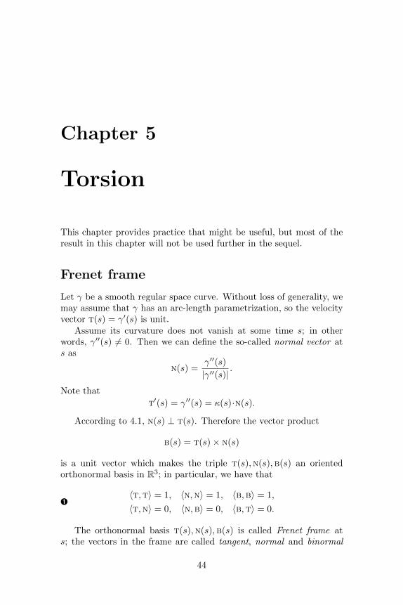
Frenet frame
Let γ be a smooth regular space curve. Without loss of generality, wemay assume that γ has an arc-length parametrization, so the velocityvector t(s) = γ′(s) is unit.
Assume its curvature does not vanish at some time s; in otherwords, γ′′(s) 6= 0. Then we can define the so-called normal vector ats as
n(s) =γ′′(s)
|γ′′(s)|.
Note that
t′(s) = γ′′(s) = κ(s)·n(s).
According to 4.1, n(s) ⊥ t(s). Therefore the vector product
b(s) = t(s)× n(s)
is a unit vector which makes the triple t(s),n(s),b(s) an orientedorthonormal basis in R3; in particular, we have that
Ê〈t,t〉 = 1, 〈n,n〉 = 1, 〈b,b〉 = 1,
〈t,n〉 = 0, 〈n,b〉 = 0, 〈b,t〉 = 0.
The orthonormal basis t(s),n(s),b(s) is called Frenet frame ats; the vectors in the frame are called tangent, normal and binormal
44

45
correspondingly. Note that the frame t(s),n(s),b(s) is defined only ifk(s) 6= 0.
The plane Πs thru γ(s) spanned by vectors t(s) and n(s) is calledosculating plane at s; equivalently it can be defined as a plane thruγ(s) that is perpendicular to the binormal vector b(s). This is theunique plane that has second order of contact with γ at s; that is,ρ(`) = o(`2), where ρ(`) denotes the distance from γ(s+ `) to Πs.
Torsion*
Let γ be a smooth unit-speed space curve and t(s),n(s),b(s) is itsFrenet frame. The value
τ(s) = 〈n′(s),b(s)〉
is called the torsion of γ at s.Note that the torsion τ(s) is defined if κ(s) 6= 0. Indeed, if κ(s) 6=
0, then Frenet frame t(s),n(s),b(s) is defined at s. Moreover sincethe function s 7→ κ(s) is continuous, it must be positive in an openinterval containing s; therefore the Frenet frame is also defined in thisinterval. Clearly t(s), n(s) and b(s) depend smoothly on s in theirdomains of definition. Therefore n′(s) is defined and so is the torsionτ(s) = 〈n′(s),b(s)〉.
The torsion measures how fast the osculating plane rotates whenone travels along γ.
5.1. Exercise. Given real numbers a and b, calculate curvature andtorsion of the helix
γa,b(t) = (a· cos t, a· sin t, b·t).
Conclude that for any κ > 0 and τ there is a helix with constantcurvature κ and torsion τ .
Frenet formulas*
Assume the Frenet frame t(s),n(s),b(s) of a curve γ is defined at s.Recall that
Ë t′(s) = κ(s)·n(s).
It is convenient to write the remaining derivatives n′(s) and b′(s) inthe frame t(s),n(s),b(s).

46 CHAPTER 5. TORSION
First let us show that
Ì n′(s) = −κ(s)·t(s) + τ(s)·b(s).
Since the frame t(s),n(s),b(s) is orthonormal, the above formulais equivalent to the following three identities:
Í 〈n′,t〉 = −κ, 〈n′,n〉 = 0, 〈n′,b〉 = τ,
The last identity follows from the definition of torsion. The second onecomes from differentiating 〈n,n〉 = 1 in Ê. Differentiating the identity〈t,n〉 = 0 in Ê; we get
〈t′,n〉+ 〈t,n′〉 = 0.
Applying Ë, we get get the first one.Differentiating the third identity in Ê, we get that b′ ⊥ b. Further
taking derivatives of the other identities with b in Ê, we get that
〈b′,t〉 = −〈b,t′〉 = −κ·〈b,n〉 = 0
〈b′,n〉 = −〈b,n′〉 = τ
Since the frame t(s),n(s),b(s) is orthonormal, it follows that
Î b′(s) = −τ(s)·n(s).
The equations Ë, Ì and Î are called Frenet formulas. All threecan be written as one matrix identity:t′
n′
b′
=
0 κ 0−κ 0 τ0 −τ 0
·tnb
.
5.2. Exercise. Deduce the formula Î from Ë and Ì by differentiatingthe identity b = t× n.
5.3. Exercise. Let γ be a regular space curve with nonvanishing cur-vature. Show that γ lies in a plane if and only if its torsion vanishes.
5.4. Exercise. Let γ be a smooth regular space curve, κ and τ itscurvature and torsion, and t,n,b its Frenet frame. Show that
b =γ′ × γ′′
|γ′ × γ′′|.
Use this formula to show that
τ =〈γ′ × γ′′, γ′′′〉|γ′ × γ′′|2
.

47
Curves of constant slope*
We say that a smooth regular space curve γ has constant slope if itsvelocity vector makes a constant angle with a fixed direction. Thefollowing theorem was proved by Michel Ange Lancret [22] more thantwo centuries ago.
5.5. Theorem. Let γ be a smooth regular curve; denote by κ andτ its curvature and torsion. Suppose κ(s) > 0 for all s. Then γ hasconstant slope if and only if the ratio τ
κ is constant.
The theorem can be proved using the Frenet formulas. The follow-ing exercise will guide you thru the proof of the theorem.
5.6. Exercise. Let γ be a smooth regular space curve with nonva-nishing curvature, t,n,b its Frenet frame and κ, τ its curvature andtorsion.
(a) Assume that 〈w,t〉 is constant for a fixed nonzero vector w.Show that
〈w,n〉 = 0.
Use it to show that
〈w,−κ·t + τ ·b〉 = 0.
Use these two identities to show that τκ is constant; it proves the
“only if” part of the theorem.(b) Assume τ
κ is constant, show that the vector w = τκ ·t + b is
constant. Conclude that γ has constant slope; it proves the “if”part of the theorem.
Let γ be a smooth unit-speed curve and s0 a fixed real number.Then the curve
α(s) = γ(s) + (s0 − s)·γ′(s)is called the evolvent of γ. Note that if `(s) denotes the tangent lineto γ at s, then α(s) ∈ `(s) and α′(s) ⊥ ` for all s.
5.7. Exercise. Show that the evolvent of a constant slope curve is aplane curve.
Spherical curves*
5.8. Theorem. A smooth regular space curve γ lies in a unit sphereif and only if the following identity∣∣∣∣κ′τ
∣∣∣∣ = κ·√κ2 − 1.

48 CHAPTER 5. TORSION
holds for its curvature κ and torsion τ .
Note that the identity implicitely implies that the torsion τ ofthe curve is nonzero; otherwise the left hand side would be undefinedwhile right hand side is defined. The proof is another application ofthe Frenet formulas; we present it in form of a guided exercise:
5.9. Exercise. Suppose γ is a smooth unit-speed space curve. Denoteby t,n,b its Frenet frame and by κ, τ its curvature and torsion.
Assume that γ is spherical; that is, |γ(s)| = 1 for any s. Show that(a) 〈t, γ〉 = 0; conclude that 〈n, γ〉2 + 〈b, γ〉2 = 1.(b) 〈n, γ〉 = − 1
κ ;(c) 〈b, γ〉′ = τ
κ .(d) Use (c) to show that if γ is closed, then τ(s) = 0 for some s.(e) Use (a)–(c) to show that∣∣∣∣κ′τ
∣∣∣∣ = κ·√κ2 − 1.
It proves the “only if” part of the theorem.
Now assume that γ is a space curve that satisfies the idenity in (e).
(f) Show that p = γ+ 1κ ·n+ κ′
κ2 ·τ ·b is constant; conclude that γ liesin the unit sphere centered at p.
It proves the “if” part of the theorem.
For a unit-speed curve γ with nonzero curvature and torsion at s,the sphere Σs with center
p(s) = γ(s) + 1κ(s) ·n(s) + κ′(s)
κ2(s)·τ(s) ·b(s)
and passing thru γ(s) is called the osculating sphere of γ at s. This isthe unique sphere that has third order of contact with γ at s; that is,ρ(`) = o(`3), where ρ(`) denotes the distance from γ(s+ `) to Σs.
Fundamental theorem of space curves*
5.10. Theorem. Let κ(s) and τ(s) be two smooth real valued func-tions defined on a real interval I. Suppose κ(s) > 0 for all s. Thenthere is a smooth unit-speed curve γ : I→ R3 with curvature κ(s) andtorsion τ(s) for every s. Moreover γ is uniquely defined up to a rigidmotion of the space.
The proof is an application of the theorem on existence and unique-ness of a solution of ordinary differential equation (B.1).
49
Proof. Fix a parameter value s0, a point γ(s0) and an oriented or-thonormal frame t(s0), n(s0), b(s0).
Consider the following system of differential equationsγ′ = t,
t′ = κ·n,n′ = −κ·t + τ ·b,b′ = −τ ·n.
with the initial condition γ(s0) and an oriented orthonormal framet(s0), n(s0), b(s0). (The system of equations has four vector equa-tions, so it can be rewritten as a system of 12 scalar equations.)
By B.1, this system has a unique solution which is defined in amaximal subinterval J ⊂ I containing s0; we need to show that actuallyJ = I.
Note that
〈t,t〉′ = 2·〈t,t′〉 = 2·κ·〈t,n〉 = 0,
〈n,n〉′ = 2·〈n,n′〉 = −2·κ·〈n,t〉+ 2·τ ·〈n,b〉 = 0,
〈b,b〉′ = 2·〈b,b′〉 = −2·τ〈b,n〉 = 0,
〈t,n〉′ = 〈t′,n〉+ 〈t,n′〉 = κ·〈n,n〉 − κ·〈t,t〉+ τ ·〈t,b〉 = 0,
〈n,b〉′ = 〈n′,b〉+ 〈n,b′〉 = 0,
〈b,t〉′ = 〈b′,t〉+ 〈b,t′〉 = −τ ·〈n,t〉+ κ·〈b,n〉 = 0.
That is, the values 〈t,t〉, 〈n,n〉, 〈b,b〉, 〈t,n〉, 〈t,n〉, 〈b,t〉 are con-stant functions of s. Since we choose t(s0), n(s0), b(s0) to be anoriented orthonormal frame, we have that the triple t(s), n(s), b(s) isan oriented orthonormal for any s. In particular, |γ′(s)| = 1 for all s.
Assume J I. Then an end of J, say a, lies in the interior of I. ByTheorem B.1, at least one of the values γ(s), t(s), n(s), b(s) escapesto infinity as s→ a. But this is impossible since the vectors t(s), n(s),b(s) remain unit and |γ′(s)| = |t(s)| = 1 — a contradiction. HenceJ = I.
It remains to prove the last statement.Assume there are two curves γ1 and γ2 with the given curvature
and torsion functions. Applying a motion of the space we can assumethat the γ1(s0) = γ2(s0) and the Frenet frames of the curves coincideat s0. Then γ1 = γ2 by uniqueness of solutions of the system (B.1).
5.11. Exercise. Assume a curve γ : R→ R3 has constant curvatureand torsion. Show that γ is a helix, possibly degenerate to a circle;that is, in a suitable coordinate system we have
γ(t) = (a· cos t, a· sin t, b·t)

50 CHAPTER 5. TORSION
for some constants a and b.
5.12. Advanced exercise. Let γ be a smooth regular space curvesuch that the distance |γ(t)− γ(t+ `)| depends only on `. Show that γis a helix, possibly degenerate to a line or a circle.

Chapter 6
Signed curvature
Suppose γ is a smooth unit-speed plane curve, so t(s) = γ′(s) is itsunit tangent vector for any s.
Let us rotate t(s) by the angle π2 counterclockwise; denote the
obtained vector by n(s). The pair t(s),n(s) is an oriented orthonormalframe in the plane which is analogous to the Frenet frame defined onpage 45; we will keep the name Frenet frame for it.
Recall that γ′′(s) ⊥ γ′(s) (see 4.1). Therefore
Ê t′(s) = k(s)·n(s).
for some real number k(s); the value k(s) is called signed curvature ofγ at s. We may use notation k(s)γ if we need to specify the curve γ.
Note that
κ(s) = |k(s)|;
that is, up to sign, the signed curvature k(s) equals the curvature κ(s)of γ at s defined on page 27; the sign tells us in which direction itturns — if γ is turning left at time s, then k(s) > 0. If we want toemphasise that we are working with the nonsigned curvature of thecurve, we call it absolute curvature.
Note that if we reverse the parametrization of γ or change theorientation of the plane, then the signed curvature changes its sign.
Since t(s),n(s) is an orthonormal frame, we have
〈t,t〉 = 1, 〈n,n〉 = 1, 〈t,n〉 = 0,
Differentiating these idenitites we get
〈t′,t〉 = 0, 〈n′,n〉 = 0, 〈t′,n〉+ 〈t,n′〉 = 0,
51

52 CHAPTER 6. SIGNED CURVATURE
By Ê, 〈t′,n〉 = k and therefore 〈t,n′〉 = −k. Whence we get
Ë n′(s) = −k(s)·t(s).
The equations Ê and Ë are the Frenet formulas for plane curves. Theycan be written in matrix form as:(
t′
n′
)=
(0 k−k 0
)·(tn
).
6.1. Exercise. Let γ0 : [a, b] → R2 be a smooth regular curve and tits tangent indicatrix. Consider another curve γ1 : [a, b]→ R2 definedby γ1(t) = γ0(t) + t(t). Show that
length γ0 6 length γ1.
The curves γ0 and γ1 in the exercise above describe the tracks ofan idealized bicycle with distance 1 from the rear to the front wheel.Thus by the exercise, the front wheel must have longer track. For moreon the geometry of bicycle tracks, see [14] and the references therein.
Fundamental theorem of plane curves
6.2. Theorem. Let k(s) be a smooth real valued function defined ona real interval I. Then there is a smooth unit-speed curve γ : I → R2
with signed curvature k(s). Moreover, γ is uniquely defined up to arigid motion of the plane.
This is the fundamental theorem of plane curves; it is a directanalog of 5.10 and it can be proved along the same lines. We presenta slightly simpler proof.
Proof. Fix s0 ∈ I. Consider the function
θ(s) =
s∫s0
k(t)·dt.
Note that by the fundamental theorem of calculus, we have θ′(s) == k(s) for all s.
Sett(s) = (cos[θ(s)], sin[θ(s)])
and let n(s) be its counterclockwise rotation by angle π2 ; so
n(s) = (− sin[θ(s)], cos[θ(s)]).
53
Consider the curve
γ(s) =
s∫s0
t(s)·ds.
Since |γ′| = |t| = 1, the curve γ is unit-speed and t,n is its Frenetframe.
Note that
γ′′(s) = t′(s) =
= (cos[θ(s)]′, sin[θ(s)]′) =
= θ′(s)·(− sin[θ(s)], cos[θ(s)]) =
= k(s)·n(s).
So k(s) is the signed curvature of γ at s. This proves the existence.
it remains to prove uniqueness. Assume γ1 and γ2 are two curvesthat satisfy the assumptions of the theorem. Applying a rigid mo-tion, we can assume that γ1(s0) = γ2(s0) = 0 and the Frenet frame ofboth curves at s0 is formed by the coordinate frame (1, 0), (0, 1). Letus denote by t1,n1 and t2,n2 the Frenet frames of γ1 and γ2 corre-spondingly. The triples γi,ti,ni satisfy the same system of ordinarydifferential equations
γ′i = ti,
t′i = k·ni,n′i = −k·ti.
Moreover, they have the same initial values at s0. By TheoremB.1, γ1 = γ2.
Note that from the proof of theorem we obtain the following corol-lary:
6.3. Corollary. Let γ : I → R2 be a smooth unit-speed curve ands0 ∈ I. Denote by k the signed curvature of γ. Assume an oriented(x, y)-coordinate system is chosen in such a way that γ(s0) is the originand γ′(s0) points in the direction of the x-axis. Then
γ′(s) = (cos[θ(s)], sin[θ(s)]),
for all s, where
θ(s) =
s∫s0
k(t)·dt.

54 CHAPTER 6. SIGNED CURVATURE
Total signed curvature
Let γ : I → R2 be a smooth unit-speed plane curve. The total signedcurvature of γ, denoted by Ψ(γ), is defined as the integral of its signedcurvature;
Ì Ψ(γ) =
∫I
k(s)·ds,
where k denotes the signed curvature of γ.If I = [a, b], then
Í Ψ(γ) = θ(b)− θ(a),
where θ is as in 6.3.If γ is a piecewise smooth and regular plane curve, then we define
its total signed curvature as the sum of the total signed curvatures ofits arcs plus the sum of the signed external angles at its joints; it ispositive if γ turns left, negative if γ turns right, 0 if it goes straight. Itis undefined if it turns exactly backward; that is, the curve has a cusp.undefined if it turns exactly backward. That is, if γ is a concatenationof smooth and regular arcs γ1, . . . , γn, then
Ψ(γ) = Ψ(γ1) + · · ·+ Ψ(γn) + θ1 + · · ·+ θn−1
where θi is the signed external angle at the joint between γi and γi+1.If γ is closed, then the concatenation is cyclic and
Ψ(γ) = Ψ(γ1) + · · ·+ Ψ(γn) + θ1 + · · ·+ θn,
where θn is the signed external angle at the joint between γn and γ1.Since
∣∣∫ k(s)·ds∣∣ 6 ∫ |k(s)|·ds, we have
Î |Ψ(γ)| 6 Φ(γ)
for any smooth regular plane curve γ; that is, total signed curvaturecan not exceed total curvature by absolute value. Note that the equal-ity holds if and only if the signed curvature does not change the sign.
Trochoid is a curve traced out by a point fixed to a wheel as it rollsalong a straight line.
6.4. Exercise. Consider the family of trochoids γa : [0, 2·π] → R2
defined byγa(t) = (t+ a· sin t, a· cos t).
(a) Given a ∈ R, find Ψ(γa) if it is defined.

55
Trochoids γa for different values a.
(b) Given a ∈ R, find Φ(γa).
6.5. Proposition. The total signed curvature of any closed simplesmooth regular plane curve γ is ±2·π; it is +2·π if the region boundedby γ lies on the left from it and −2·π otherwise.
Moreover the same statement holds for any closed piecewise simplesmooth regular plane curve γ if its total signed curvature is defined.
This proposition is called sometimes Umlaufsatz ; it is a differential-geometric analog of the theorem about the sum of the internal anglesof a polygon (E.1) which we use in the proof. A more conceptual proofwas given by Heinz Hopf [17], [18, p. 42].
Proof. Without loss of generality we may assume that γ is oriented insuch a way that the region bounded by γ lies on the left from it. Wecan also assume that it is parametrized by arc-length.
Consider a closed polygonal line β = p1 . . . pn inscribed in γ. Wecan assume that the arcs between the vertexes are sufficiently small;in this case the polygonal line is simple and each arc γi from pi to pi+1
has small total absolute curvature, say Φ(γi) < π for each i.
α1
αn
β1
β2
δ1
δ2
p1
p2
. ..
pn
As usual we use indexes modulo n,in particular pn+1 = p1. Assume pi =γ(ti). Set
wi = pi+1 − pi, vi = γ′(ti),
αi = ](vi,wi), βi = ](wi−1,vi),
where αi, βi ∈ (−π, π] are signed angles— αi is positive if wi points to the leftfrom vi.
By Í, the value
Ï Ψ(γi)− αi − βi+1
56 CHAPTER 6. SIGNED CURVATURE
is a multiple of 2·π. Since Φ(γi) < π, by the chord lemma (4.11), wealso have that |αi| + |βi| < π. By Î, we have that |Ψ(γi)| 6 Φ(γi);therefore the value in Ï vanishes. In other word, the equality
Ψ(γi) = αi + βi+1
holds for each i.Note that
Ð δi = π − αi − βi
is the internal angle of β at pi; δi ∈ (0, 2·π) for each i. Recall that thesum of the internal angles of an n-gon is (n− 2)·π (see E.1); that is,
δ1 + · · ·+ δn = (n− 2)·π.
Therefore
Ñ
Ψ(γ) = Ψ(γ1) + · · ·+ Ψ(γn) =
= (α1 + β2) + · · ·+ (αn + β1) =
= (β1 + α1) + · · ·+ (βn + αn) =
= (π − δ1) + · · ·+ (π − δn) =
= n·π − (n− 2)·π =
= 2·π.
The case of piecewise smooth and regular curves is done the sameway; we need to subdivide the arcs in the cyclic concatenation furtherto meet the requirement above and instead of equation Ð we have
δi = π − αi − βi − θi,
where θi is the signed external angle of γ at pi; it vanishes if the curveγ is smooth at pi. Therefore instead of equation Ñ, we have
Ψ(γ) = Ψ(γ1) + · · ·+ Ψ(γn) + θ1 + · · ·+ θn =
= (α1 + β2) + · · ·+ (αn + β1) =
= (β1 + α1 + θ1) + · · ·+ (βn + αn + θn) =
= (π − δ1) + · · ·+ (π − δn) =
= n·π − (n− 2)·π =
= 2·π.
6.6. Exercise. Draw a smooth regular closed plane curve γ such that(a) Ψ(γ) = 0;

57
(b) Ψ(γ) = Φ(γ) = 10·π;(c) Ψ(γ) = 2·π and Φ(γ) = 4·π.
6.7. Exercise. Let γ : [a, b]→ R be a smooth regular plane curve withFrenet frame t,n. Given a real parameter `, consider the curve γ`(t) =γ(t) + `·n(t); it is called a parallel curve of γ at signed distance `.
(a) Show that γ` is a regular curve if `·k(t) 6= 1 for all t, where k(t)denotes the signed curvature of γ.
(b) Set L(`) = length γ`. Show that
Ò L(`) = L(0)− `·Ψ(γ)
for all ` sufficiently close to 0.(c) Describe an example showing that formula Ò does not hold for
all `.
Osculating circline
6.8. Proposition. Given a point p, a unit vector t and a real numberk, there is a unique smooth unit-speed curve σ : R→ R2 that starts atp in the direction of t and has constant signed curvature k.
Moreover, if k = 0, then σ(s) = p+ s·t which runs along a line; ifk 6= 0, then σ runs around the circle of radius 1
|k| and center p+ 1k ·n,
where t,n is an oriented orthonoral frame.
Further we will use the term circline for a circle or a line; theseare the only plane curves with constant signed curvature.
Proof. The proof is done by a calculation based on 6.2 and 6.3.Suppose s0 = 0, choose a coordinate system such that p is its origin
and t points in the direction of the x-axis. Therefore n points in thedirection of the y-axis. Then
θ(s) =
s∫0
k·dt =
= k·s.
Thereforeσ′(s) = (cos[k·s], sin[k·s]).
It remains to integrate the last identity. If k = 0, we get
σ(s) = (s, 0)

58 CHAPTER 6. SIGNED CURVATURE
which describes the line σ(s) = p+ s·t.If k 6= 0, we get
σ(s) = ( 1k · sin[k·s], 1
k ·(1− cos[k·s])).
which is the circle of radius r = 1|k| centered at (0, 1
k ) = p+ 1k ·n.
γ
σ6.9. Definition. Let γ be a smooth unit-speedplane curve; denote by k(s) the signed curvatureof γ at s.
The unit-speed curve σ of constant signedcurvature k(s) that starts at γ(s) in the direc-tion γ′(s) is called the osculating circline of γat s.
The center and radius of the osculating cir-cle at a given point are called center of curvature and radius of cur-vature of the curve at that point.
The osculating circle σs can be also defined as the unique circlinethat has second order of contact with γ at s; that is, ρ(`) = o(`2),where ρ(`) denotes the distance from γ(s+ `) to σs.
The following exercise would is recommended to the reader familiarwith the notion of inversion.
6.10. Advanced exercise. Suppose γ is a smooth regular planecurve that does not pass thru the origin. Let γ be the inversion ofγ in the unit circle centered at the origin. Show that osculating cir-cline of γ at s is the inversion of osculating circline of γ at s.
Spiral lemma
The following lemma was proved by Peter Tait [36] and later rediscov-ered by Adolf Kneser [19].
6.11. Lemma. Assume that γ is a smooth regular plane curve withstrictly decreasing positive signed curvature. Then the osculating cir-cles of γ are nested; that is, if σs denoted the osculating circle of γ ats, then σs0 lies in the open disc bounded by σs1 for any s0 < s1.
It turns out that the osculating circles of thecurve γ give a peculiar foliation of an annulusby circles; it has the following property: if asmooth function is constant on each osculatingcircle it must be constant in the annulus [see15, Lecture 10]. Also note that the curve γ is
59
tangent to a circle of the foliation at each of itspoints. However, it does not run along any of
those circles.
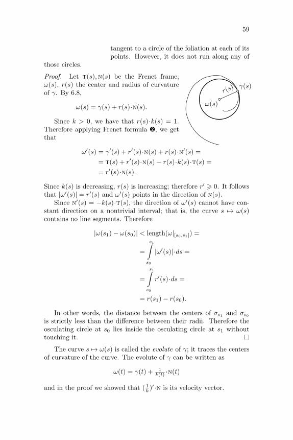
γ(s)
ω(s)
r(s)
Proof. Let t(s),n(s) be the Frenet frame,ω(s), r(s) the center and radius of curvatureof γ. By 6.8,
ω(s) = γ(s) + r(s)·n(s).
Since k > 0, we have that r(s)·k(s) = 1.Therefore applying Frenet formula Ë, we getthat
ω′(s) = γ′(s) + r′(s)·n(s) + r(s)·n′(s) =
= t(s) + r′(s)·n(s)− r(s)·k(s)·t(s) =
= r′(s)·n(s).
Since k(s) is decreasing, r(s) is increasing; therefore r′ > 0. It followsthat |ω′(s)| = r′(s) and ω′(s) points in the direction of n(s).
Since n′(s) = −k(s)·t(s), the direction of ω′(s) cannot have con-stant direction on a nontrivial interval; that is, the curve s 7→ ω(s)contains no line segments. Therefore
|ω(s1)− ω(s0)| < length(ω|[s0,s1]) =
=
s1∫s0
|ω′(s)|·ds =
=
s1∫s0
r′(s)·ds =
= r(s1)− r(s0).
In other words, the distance between the centers of σs1 and σs0is strictly less than the difference between their radii. Therefore theosculating circle at s0 lies inside the osculating circle at s1 withouttouching it.
The curve s 7→ ω(s) is called the evolute of γ; it traces the centersof curvature of the curve. The evolute of γ can be written as
ω(t) = γ(t) + 1k(t) ·n(t)
and in the proof we showed that ( 1k )′ ·n is its velocity vector.

60 CHAPTER 6. SIGNED CURVATURE
6.12. Exercise. Show that the stretched as-troid
ω(t) = (a2−b2a · cos3 t, b
2−a2b · sin3 t)
is an evolute of the ellipse defined by
γ(t) = (a· cos t, b· sin t).
The following theorem states formally that if you drive on the planeand turn the steering wheel to the left all the time, then you will notbe able to come back to the same place.
6.13. Theorem. Assume γ is a smooth regular plane curve withpositive and strictly monotonic signed curvature. Then γ is simple.
The same statement holds without assuming positivity of curva-ture; the proof requires only minor modifications.
Proof of 6.13. Note that γ(s) lies on the osculating circle σs of γ at s.If s1 6= s0, then by lemma 6.11, σs0 does not intersect σs1 . Thereforeγ(s1) 6= γ(s0), hence the result.
6.14. Exercise. Show that a 3-dimensional analog of the theoremdoes not hold. That is, there are self-intersecting smooth regular spacecurves with strictly monotonic curvature.
6.15. Exercise. Assume that γ is a smooth regular plane curve withpositive strictly monotonic signed curvature.
(a) Show that no line can be tangent to γ at two distinct points.(b) Show that no circle can be tangent to γ at three distinct points.
Note that part (6.15a) does not hold if weallow the curvature to be negative; an exam-ple is shown on the diagram.

Chapter 7
Supporting curves
Cooriented tangent curves
Suppose γ1 and γ2 are smooth regular plane curves. Recall that thecurves γ1 and γ2 are tangent at the time parameters t1 and t2 ifγ1(t1) = γ2(t2) and they share the tangent line at these time pa-rameters.
In this case the point p = γ1(t1) = γ2(t2) is called a point oftangency of the curves. If both curves are simple, then we may saythat γ1 and γ2 are tangent at the point p without ambiguity.
Note that if γ1 and γ2 are tangent at the time parameters t1 andt2, then the velocity vectors γ′1(t1) and γ′2(t2) are parallel. If γ′1(t1)
cooriented controriented
γ1
γ2
γ1
γ2
p p
and γ′2(t2) point in the same direction we say that the curves arecooriented, if these directions are opposite, we say that the curves arecontroriented.
Note that reverting the parametrization of one of the curves, coori-ented curves become counteroriented and vice versa; so we can alwaysassume that the curves are cooriented at a given point of tangency.
61

62 CHAPTER 7. SUPPORTING CURVES
Supporting curves
Let γ1 and γ2 be two smooth regular plane curves that share a point
p = γ1(t1) = γ2(t2)
which is not an endpoint of any of the curves. Suppose that there isε > 0 such that the arc γ2|[t2−ε,t2+ε] lies in a closed plane region Rwith the arc γ1|[t1−ε,t1+ε] in its boundary, then we say that γ1 locallysupports γ2 at the time parameters t1 and t2. If both curves aresimple, then we also could say that γ1 locally supports γ2 at the pointp without ambiguity.
p
γ2
γ1
RRRRRRRRRRRRRRRRRRRRRRRRRRRRRRRRRRRRRRRRRRRRRRRRRRRRRRRRRRRRRRRRR
If γ1 is simple proper curve, so itdivides the plane into two closed regionthat lie on left and right from γ1, thenwe say that γ1 globally supports γ2 at t2if γ2 runs in one of these closed regionsand γ2(t2) lies on γ.
If γ2 is a closed curve so it dividesthe plane into two regions a boundedinside and unbounded outside. In this
case we say if γ1 supports γ2 from inside (from outside) if γ1 supportsγ2 and in the region inside it (correspondingly outside it).
Note that if γ1 and γ2 share a point p = γ1(t1) = γ2(t2) and nottangent at t1 and t2, then γ2 crosses γ1 at t2 moving from one of itssides to the other. It follows that γ1 can not locally support γ2 at thetime parameters t1 and t2. Whence we get the following:
7.1. Definition-Observation. Let γ1 and γ2 be two smooth regularplane curves. Suppose γ1 locally supports γ2 at time parameters t1 andt2. Then γ1 is tangent to γ2 at t1 and t2.
In particular, we could say if γ1 and γ2 are coorineted or controri-ented at at the time parameters t1 and t2. If the curves are coorienatedand the region R in the definition of supporting curves lie on the right(left) from the arc of γ1, then we say that γ1 supports γ2 from the left(correspondingly right).
If the curves on the diagram oriented according the arrows, thenγ1 supports γ2 from the right at p (as well as γ2 supports γ1 from theleft at p).
We say that a smooth regular plane curve γ has a vertex at s if thesigned curvature function is critical at s; that is, if k′(s)γ = 0. If γ issimple we could say that the point p = γ(s) is a vertex of γ withoutambiguity.

63
7.2. Exercise. Assume that osculating circle σs of a smooth regularsimple plane curve γ locally supports γ at p = γ(s). Show that p is avertex of γ.
Supporting test
The following proposition resembles the second derivative test.
7.3. Proposition. Let γ1 and γ2 be two smooth regular plane curves.Suppose γ1 locally supports γ2 from the left (right) at the time
parameters t1 and t2. Then
k1(t1) 6 k2(t2) (correspondingly k1(t1) > k2(t2)).
where k1 and k2 denote the signed curvature of γ1 and γ2 correspond-ingly.
A partial converse also holds. Namely, if γ1 and γ2 tangent andcooriented at the time parameters t1 and t2 then γ1 locally supports γ2
from the left (right) at the time parameters t1 and t2 if
k1(t1) < k2(t2) (correspondingly k1(t1) > k2(t2)).
Proof. Without loss of generality, we can assume that t1 = t2 = 0, theshared point γ1(0) = γ2(0) is the origin and the velocity vectors γ′1(0),γ′2(0) point in the direction of x-axis.
Note that small arcs of γ1|[−ε,+ε] and γ2|[−ε,+ε] can be describedas a graph y = f1(x) and y = f2(x) for smooth functions f1 and f2
such that fi(0) = 0 and f ′i(0) = 0. Note that f ′′1 (0) = k1(0) andf ′′2 (0) = k2(0) (see 4.4)
Clearly, γ1 supports γ2 from the left (right) if
f1(x) 6 f2(x) (correspondingly f1(x) > f2(x))
for all sufficiently small values x. Applying the second derivative test,we get the result.
7.4. Advanced exercise. Let γ0 and γ1 be two smooth unit-speedsimple plane curves that are tangent and cooriented at the point p == γ0(0) = γ1(0). Assume k0(s) 6 k1(s) for any s. Show that γ0 locallysupports γ1 from the right at p.
Give an example of two proper curves γ0 and γ1 satisfying the abovecondition such that γ0 does not globally support γ1 at p.

64 CHAPTER 7. SUPPORTING CURVES
Note that according to the DNA inequality (4.23) for any closedsmooth regular curve that runs in a unit disc, the average of its ab-solute curvature at least 1; in particular it has a point with absolutecurvature at lest 1. The following exercise says that the last statementholds for loops.
7.5. Exercise. Assume a closed smooth regular plane loop γ runs ina unit disc. Show that there is a point on γ with absolute curvature atleast 1.
7.6. Exercise. Assume a closed smooth regular plane curve γ runsbetween parallel lines on distance 2 from each other. Show that thereis a point on γ with absolute curvature at least 1.
Try to prove the same for a smooth regular plane loop.
7.7. Exercise. Assume a closed smooth regular plane curve γ runsinside of a triangle 4 with inradius 1; that is, the inscribed circle of 4has radius 1. Show that there is a point on γ with absolute curvatureat least 1.
The exercise above is a baby case of a 7.15.
y x
FFFFFFFFFFFFFFFFFFFFFFFFFFFFFFFFFFFFFFFFFFFFFFFFFFFFFFFFFFFFFFFFF
σ2
σ1
γγγγγγγγγγγγγγγγγγγγγγγγγγγγγγγγγγγγγγγγγγγγγγγγγγγγγγγγγγγγγγγγγ
7.8. Exercise. Let F be a plane figurebounded by two circle arcs σ1 and σ2 of signedcurvature 1 that run from x to y. Suppose σ1
is a shorter than σ2. Assume a simple arc γruns in F and has the end points on σ1. Showthat the absolute curvature of γ is at least 1at some parameter value.
Convex curves
Recall that a plane curve is convex if it bounds a convex region.
7.9. Proposition. Suppose that a closed simple plane curve γ boundsa figure F . Then F is convex if and only if the signed curvature of γdoes not change sign.
7.10. Lens lemma. Let γ be a smooth regular simple plane curvethat runs from x to y. Assume that γ runs on the right side (corre-spondingly left side) of the oriented line xy and only its endpoints xand y lie on the line. Then γ has a point with positive (correspondinglynegative) signed curvature.
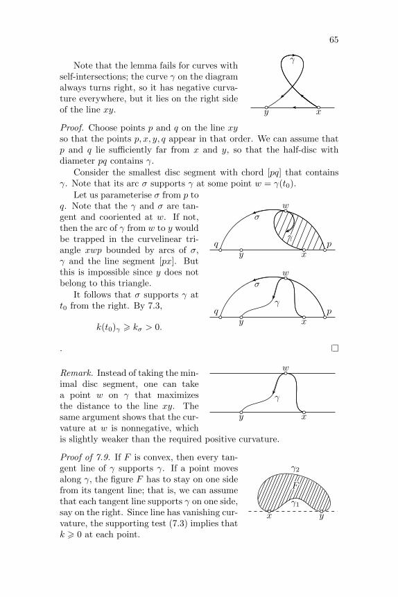
65
xy
γNote that the lemma fails for curves with
self-intersections; the curve γ on the diagramalways turns right, so it has negative curva-ture everywhere, but it lies on the right sideof the line xy.
Proof. Choose points p and q on the line xyso that the points p, x, y, q appear in that order. We can assume thatp and q lie sufficiently far from x and y, so that the half-disc withdiameter pq contains γ.
Consider the smallest disc segment with chord [pq] that containsγ. Note that its arc σ supports γ at some point w = γ(t0).
xypq
w
γγγγγγγγγγγγγγγγγγγγγγγγγγγγγγγγγγγγγγγγγγγγγγγγγγγγγγγγγγγγγγγγγ
σ
xypq
w
γ
σ
Let us parameterise σ from p toq. Note that the γ and σ are tan-gent and cooriented at w. If not,then the arc of γ from w to y wouldbe trapped in the curvelinear tri-angle xwp bounded by arcs of σ,γ and the line segment [px]. Butthis is impossible since y does notbelong to this triangle.
It follows that σ supports γ att0 from the right. By 7.3,
k(t0)γ > kσ > 0.
.
xy
w
γ
Remark. Instead of taking the min-imal disc segment, one can takea point w on γ that maximizesthe distance to the line xy. Thesame argument shows that the cur-vature at w is nonnegative, whichis slightly weaker than the required positive curvature.
FFFFFFFFFFFFFFFFFFFFFFFFFFFFFFFFFFFFFFFFFFFFFFFFFFFFFFFFFFFFFFFFF
x y
γ1
γ2
Proof of 7.9. If F is convex, then every tan-gent line of γ supports γ. If a point movesalong γ, the figure F has to stay on one sidefrom its tangent line; that is, we can assumethat each tangent line supports γ on one side,say on the right. Since line has vanishing cur-vature, the supporting test (7.3) implies thatk > 0 at each point.

66 CHAPTER 7. SUPPORTING CURVES
Denote by K the convex hull of F . If F is not convex, then F is aproper subset of K. Therefore ∂K contains a line segment that is nota part of ∂F . In other words, there is a line that supports γ at twopoints, say x and y that divide γ in two arcs γ1 and γ2, both distinctfrom the line segment [x, y].
Note the one of the arcs γ1 or γ2 is parametrized from x to yand the other from y to x. Passing to a smaller arc if necessary wecan ensure that only its endpoints lie on the line. Applying the lenslemma, we get that the arcs γ1 and γ2 contain points with curvaturesof opposite signs.
That is, if F is not convex, then curvature of γ changes sign. Equiv-alently: if curvature of γ does not change sign, then F is convex.
7.11. Exercise. Suppose γ is a smooth regular simple closed convexplane curve of diameter larger than 2. Show that γ has a point withabsolute curvature less than 1.
7.12. Exercise. Suppose γ is a simple smooth regular curve in theplane with positive curvature. Assume γ crosses a line ` at the pointsp1, p2, . . . pn and these points appear on γ in the same order.
(a) Show that p2 cannot lie between p1 and p3 on `.
(b) Show that if p3 lies between p1 and p2 on `, then the points appearon ` in the following order:
p1, p3, . . . , p4, p2.
(c) Describe all possible orders of pi on `.
Moon in a puddle
The following theorem is a slight generalization of the theorem provedby Vladimir Ionin and German Pestov in [30]. For convex curves, thisresult was known earlier [5, §24].
7.13. Theorem. Assume γ is a simple closed smooth reg-ular plane loop with absolute curvature bounded by 1. Thenit surrounds a unit disc.
This theorem gives a simple but nontrivial example ofthe so-called local to global theorems — based on some localdata (in this case the curvature of a curve) we conclude aglobal property (in this case existence of a large disc surrounded bythe curve).

67
A straightforward approach would be tostart with some disc in the region bounded bythe curve and blow it up to maximize its ra-dius. However, as one may see from the dia-gram it does not always lead to a solution — aclosed plane curve of curvature at most 1 maysurround a disc of radius smaller than 1 thatcannot be enlarged continuously.
7.14. Key lemma. Assume γ is a simple closed smooth regular planeloop. Then at one point of γ (distinct from its base) its osculating circleσ globally support γ from the inside.
First let us show that the theorem follows from the lemma.
Proof of 7.13 modulo 7.14. Since γ has absolute curvature at most1, each osculating circle has radius at least 1. According to the keylemma one of the osculating circles σ globally support γ from inside.In particular σ lies inside of γ, whence the result.
Proof of 7.14. Denote by F the closed region surrounded by γ. Weneed to show that one osculating circle lies completely in F . Assumecontrary; that is, the osculating circle at each point p ∈ γ does not liein F .
σ1 σ2 σ3σ3σ3σ3σ3σ3σ3σ3σ3σ3σ3σ3σ3σ3σ3σ3σ3σ3σ3σ3σ3σ3σ3σ3σ3σ3σ3σ3σ3σ3σ3σ3σ3σ3σ3σ3σ3σ3σ3σ3σ3σ3σ3σ3σ3σ3σ3σ3σ3σ3σ3σ3σ3σ3σ3σ3σ3σ3σ3σ3σ3σ3σ3σ3σ3 σ3σ3σ3σ3σ3σ3σ3σ3σ3σ3σ3σ3σ3σ3σ3σ3σ3σ3σ3σ3σ3σ3σ3σ3σ3σ3σ3σ3σ3σ3σ3σ3σ3σ3σ3σ3σ3σ3σ3σ3σ3σ3σ3σ3σ3σ3σ3σ3σ3σ3σ3σ3σ3σ3σ3σ3σ3σ3σ3σ3σ3σ3σ3σ3σ3σ∞σ∞σ∞σ∞σ∞σ∞σ∞σ∞σ∞σ∞σ∞σ∞σ∞σ∞σ∞σ∞σ∞σ∞σ∞σ∞σ∞σ∞σ∞σ∞σ∞σ∞σ∞σ∞σ∞σ∞σ∞σ∞σ∞σ∞σ∞σ∞σ∞σ∞σ∞σ∞σ∞σ∞σ∞σ∞σ∞σ∞σ∞σ∞σ∞σ∞σ∞σ∞σ∞σ∞σ∞σ∞σ∞σ∞σ∞σ∞σ∞σ∞σ∞σ∞σ∞
p1 p2
p3
p∞
q1q2
q3
F
Given a point p ∈ γ let us consider the maximal circle σ that liescompletely in F and tangent to γ at p. Note that σ has to touchγ at another point; otherwise if we increase its radius r slightly theresulting circle will still stay in F . The circle σ will be called theincircle of F at p.
Fix a point p1 and let σ1 be the incircle at p1. Denote by γ1 anarc of γ from p1 to a first point q1 on σ1. Denote by σ1 and σ1 twoarcs of σ1 from p1 to q1 such that the cyclic concatenation of σ1 andγ1 surrounds σ1.
Let p2 be the midpoint of γ1 and σ2 be the incircle at p2.

68 CHAPTER 7. SUPPORTING CURVES
y
x
p1
q1
p2
s
γ1
σ1
σ1σ1σ1σ1σ1σ1σ1σ1σ1σ1σ1σ1σ1σ1σ1σ1σ1σ1σ1σ1σ1σ1σ1σ1σ1σ1σ1σ1σ1σ1σ1σ1σ1σ1σ1σ1σ1σ1σ1σ1σ1σ1σ1σ1σ1σ1σ1σ1σ1σ1σ1σ1σ1σ1σ1σ1σ1σ1σ1σ1σ1σ1σ1σ1σ1σ2
Two ovals on the di-agram pretend to becircles.
Note that σ2 cannot intersect σ1. Other-wise, if σ2 intersects σ1 at some point s, then σ2
has to have two more common points with σ1,say x and y — one for each arc of σ2 from p2 tos. Therefore σ1 = σ2 as two circles with threecommon points: s, x, and y. On the otherhand, by construction, we have that p2 ∈ σ2
and p2 /∈ σ1 — a contradiction.Recall that σ2 has to touch γ at another
point. From above it follows that it can onlytouch γ1 and therefore we can choose an arc
γ2 ⊂ γ1 that runs from p2 to a first point q2 on σ2. Note that byconstruction we have that
Ê length γ2 <12 · length γ1.
Repeating this construction recursively, we get an infinite sequenceof arcs γ1 ⊃ γ2 ⊃ . . . ; by Ê, we also get that
length γn → 0 as n→∞.
Therefore the intersection ⋂n
γn
contains a single point; denote it by p∞.Let σ∞ be the incircle at p∞; it has to touch γ at another point,
say q∞. The same argument as above shows that q∞ ∈ γn for any n.It follows that q∞ = p∞ — a contradiction.
7.15. Exercise. Assume that a closed smooth regular curve γ liesin a figure F bounded by a closed simple plane curve. Suppose thatR is the maximal radius of discs that lies in F . Show that absolutecurvature of γ is at least 1
R at some parameter value.
Four-vertex theorem
Recall that a vertex of a smooth regular curve is definedas a critical point of its signed curvature; in particular,any local minimum (or maximum) of the signed curva-ture is a vertex. For example, every point of a circle isits vertex.
7.16. Four-vertex theorem. Any smooth regularsimple plane curve has at least four vertices.

69
Evidently any closed smooth regular curve has at least two ver-texes — where the minimum and the maximum of the curvature areattained. On the diagram the vertexes are marked; the first curve hasone self-intersection and exactly two vertexes; the second curve hasexactly four vertexes and no self-intersections.
The four-vertex theorem was first proved by Syamadas Mukhopad-hyaya [27] for convex curves. It has a number of different proofs andgeneralizations. One of my favorite proofs was given by Robert Os-serman [29]. We give another proof based on the key lemma in theprevious section. It proves the following stronger statement.
7.17. Theorem. Any smooth regular simple plane curve has is glob-ally supported by its osculating circle at least at 4 distinct points; twofrom inside and two from outside.
Proof of 7.16 modulo 7.17. First note thatif an osculating circline σ at a point p sup-ports γ locally, then p is a vertex. Indeed, ifp is not a vertex, then a small arc around phas monotonic curvature. Applying the spirallemma (6.11) we get that the osculating circlesat this arc are nested. In particular the curveγ crosses σ at p and therefore σ is does notlocally support γ at p.
Proof of 7.17. According to key lemma (7.14), there is a point p ∈ γsuch that its osculating circle supports γ from inside. The curve γ canbe considered as a loop with the base at p. Therefore the key lemmaimplies existence of another point q ∈ γ with the same property.
It shows the existence of two osculating circles that support γ frominside; it remains to show existence of two osculating circles that sup-port γ from outside.
In order to get the osculating circles supporting γ from outside,one can repeat the proof of key lemma taking instead of incircle thecircline of maximal signed curvature that supports the curve fromoutside, assuming that γ is oriented so that the region on the left fromit is bounded.
(Alternatively, if one applies to γ an inverse with the center insideγ, then the obtained curve γ1 also has two osculating circles thatsupport γ1 from inside. According to 6.10, these osculating circlinesare inverses of the circlines osculating to γ. Note that the rigion lyinginside of γ is mapped to the region outside of γ1 and the other wayaround. Therefore these two circlines correspond to the osculatingcirclines supporting γ from outside.)

70 CHAPTER 7. SUPPORTING CURVES
p1
p2...
p2·n
7.18. Advanced exercise. Suppose γ is aclosed simple smooth regular plane curve and σis a circle. Assume γ crosses σ at the pointsp1, . . . , p2·n and these points appear in the samecycle order on γ and on σ. Show that γ has atleast 2·n vertexes.
Construct an example of a closed simplesmooth regular plane curve γ with only 4 vertexes that crosses a givencircle at arbitrarily many points.

Part III
Surfaces
71

Chapter 8
Definitions
Topological surfaces
We will be mostly interested in smooth regular surfaces defined in thefollowing section. However few times we will use the following generaldefinition.
A connected subset Σ in the Euclidean space R3 is called a topo-logical surface (more precisely an embedded surface without boundary)if any point of p ∈ Σ admits a neighborhood W in Σ that can beparameterized by an open subset in the Euclidean plane; that is, thereis an injective continuous map U →W from an open set U ⊂ R2 suchthat its inverse W → U is also continuous.
Smooth surfaces
Recall that a function f of two variables x and y is called smooth if all
its partial derivatives ∂m+n
∂xm∂yn f are defined and are continuous in thedomain of definition of f .
A connected set Σ ⊂ R3 is called a smooth surface (or more pre-cisely smooth regular embedded surface) if it can be described locallyas a graph of a smooth function in an appropriate coordinate system.
More precisely, for any point p ∈ Σ one can choose a coordinatesystem (x, y, z) and a neighborhood U 3 p such that the intersectionW = U ∩ Σ is formed by a graph z = f(x, y) of a smooth function fdefined in an open domain of the (x, y)-plane.
Examples. The simplest example of a smooth surface is the (x, y)-plane
Π =
(x, y, z) ∈ R3 : z = 0.
72

73
The plane Π is a surface since it can be described as the graph of thefunction f(x, y) = 0.
All other planes are smooth surfaces as well since one can choosea coordinate system so that it becomes the (x, y)-plane. We may alsopresent a plane as a graph of a linear function f(x, y) = a·x+ b·y + cfor some constants a, b and c (assuming the plane is not perpendicularto the (x, y)-plane).
A more interesting example is the unit sphere
S2 =
(x, y, z) ∈ R3 : x2 + y2 + z2 = 1.
This set is not the graph of any function, but S2 is locally a graph; itcan be covered by the following 6 graphs:
z = f±(x, y) = ±√
1− x2 − y2,
y = g±(x, z) = ±√
1− x2 − z2,
x = h±(y, z) = ±√
1− y2 − z2,
where each function f±, g±, h± is defined in an open unit disc. Anypoint p ∈ S2 lies in one of these graphs therefore S2 is a surface. Sinceeach function is smooth, so is S2.
Surfaces with boundary
A connected subset in a surface that is bounded by one or more curvesis called surface with boundary ; the curves form the boundary line ofthe surface.
When we say surface we usually mean a smooth regular surfacewithout boundary ; we may use the terms surface without boundary ifwe need to emphasise it; otherwise we may use the term surface withpossibly nonempty boundary.
Proper, closed and open surfaces
If the surface Σ is formed by a closed set, then it is called proper. Forexample, for any smooth function f , defined on whole plane, its graphz = f(x, y) is a proper surface. The sphere S2 gives another exampleof proper surface.
On the other hand, the open disc(x, y, z) ∈ R3 : x2 + y2 < 1, z = 0
is not proper; this set is neither open nor closed.
74 CHAPTER 8. DEFINITIONS
A compact surface without boundary is called closed (this term isclosely related to closed curve but has nothing to do with closed set).
A proper noncompact surface without boundary is called open(again the term open set is not relevant).
For example, the paraboloid z = x2 +y2 is an open surface; sphereS2 is a closed surface.
Note that any proper surface without boundary is either closed oropen.
The following claim is a two-dimesional analog of 2.8; hopefully itis intuitively obvious. Its proof is not at all trivial; a standard proofuses the so-called Alexander’s duality which is a classical technique inalgebraic topology. We omit its proof since it would take us far awayfrom the main subject.
8.1. Claim. The complement of any proper topological surface with-out boundary (or, equivalently any open or closed topological surface)has exactly two connected components.
Implicitly defined surfaces
8.2. Proposition. Let f : R3 → R be a smooth function. Supposethat 0 is a regular value of f ; that is, ∇pf 6= 0 if f(p) = 0. Thenany connected component Σ of the set of solutions of the equationf(x, y, z) = 0 is a surface.
Proof. Fix p ∈ Σ. Since ∇pf 6= 0 we have
∂f∂x (p) 6= 0, ∂f
∂y (p) 6= 0, or ∂f∂z (p) 6= 0.
We may assume ∂f∂z (p) 6= 0; otherwise permute the coordinates x, y, z.
The implicit function theorem (A.2) implies that a neighborhoodof p in Σ is the graph z = h(x, y) of a smooth function h defined onan open domain in R2. It remains to apply the definition of smoothsurface (page 72).
8.3. Exercise. Describe the set of real numbers ` such that the equa-tion
x2 + y2 − z2 = `
describes a smooth regular surface.

75
Local parametrizations
Let U be an open domain in R2 and s : U → R3 be a smooth map.We say that s is regular if its Jacobian has maximal rank; in this caseit means that the vectors ∂s
∂u and ∂s∂v are linearly independent at any
(u, v) ∈ U ; equivalently ∂s∂u ×
∂s∂v 6= 0, where × denotes the vector
product.
8.4. Proposition. If s : U → R3 is a smooth regular embedding ofan open connected set U ⊂ R2, then its image Σ = s(U) is a smoothsurface.
Proof. Set
s(u, v) = (xs(u, v), ys(u, v), zs(u, v)).
Since s is regular, its Jacobian matrix
Jac s =
∂xs∂u
∂xs∂v
∂ys∂u
∂ys∂v
∂zs∂u
∂zs∂v
has rank two at any pint (u, v) ∈ U .
Fix a point p ∈ Σ; by shifting the coordinate system we may assumethat p is the origin. Permuting the coordinates x, y, z if necessary, wemay assume that the matrix(
∂xs∂u
∂xs∂v
∂ys∂u
∂ys∂v
),
is invertible. Note that this is the Jacobian matix of the map
(u, v) 7→ (xs(u, v), ys(u, v)).
The inverse function theorem implies that there is a smooth regularfunction h defined on an open set W 3 0 in the (x, y)-plane such that
(xs h)(x, y) = x and (ys h)(x, y) = y
for any (x, y) ∈ W . It follows that the graph z = zs h(x, y) for(x, y) ∈ W is a subset in Σ. Clearly this graph is open in Σ. Since pis arbitrary, we get that Σ is a surface.
If we have s and Σ as in the proposition, then we say that s is asmooth parametrization of the surface Σ.

76 CHAPTER 8. DEFINITIONS
Not all the smooth surfaces can be described by such a parametriza-tion; for example the sphere S2 cannot. But any smooth surface Σ ad-mits a local parametrization; that is, any point p ∈ Σ admits an openneighborhood W ⊂ Σ with a smooth regular parametrization s. Inthis case any point in W can be described by two parameters, usuallydenoted by u and v, which are called local coordinates at p. The maps is called a chart of Σ.
If W is a graph z = h(x, y) of a smooth function h, then the map
s : (u, v) 7→ (u, v, h(u, v))
is a chart. Indeed, s has an inverse (u, v, h(u, v)) 7→ (u, v) which iscontinuous; that is, s is an embedding. Further, ∂s
∂u = (1, 0, ∂h∂u ) and∂s∂v = (0, 1, ∂h∂v ). Whence ∂s
∂u and ∂s∂v are linearly independent; that is,
s is a regular map.Note that from 8.4, we obtain the following corollary.
8.5. Corollary. A connected set Σ ⊂ R3 is a smooth regular surfaceif and only if Σ has a local parametrization by a smooth regular mapat any point p ∈ Σ.
8.6. Exercise. Consider the following map
s(u, v) = ( 2·u1+u2+v2 ,
2·v1+u2+v2 ,
21+u2+v2 ).
Show that s is a chart of the unit sphere centered at (0, 0, 1); describethe image of s.
The map s in the exercise can be visualized using the followingmap
(u, v, 1) 7→ ( 2·u1+u2+v2 ,
2·v1+u2+v2 ,
21+u2+v2 )
which is called stereographic projection from the plane z = 1 to theunit sphere with center at (0, 0, 1) Note that the point (u, v, 1) and itsimage ( 2·u
1+u2+v2 ,2·v
1+u2+v2 ,2
1+u2+v2 ) lie on one half-line starting at theorigin.
Let γ(t) = (x(t), y(t)) be a planecurve. Recall that the surface of revolu-tion of the curve γ around the x-axis canbe described as the image of the map
(t, θ) 7→ (x(t), y(t)· cos θ, y(t)· sin θ).
For fixed t or θ the obtained curves arecalled meridian or correspondingly paral-lel of the surface; note that parallels are

77
formed by circles in the plane perpendic-ular to the axis of rotation.
8.7. Exercise. Assume γ is a closed simple smooth regular planecurve that does not intersect the x-axis. Show that surface of revolutionof γ around the x-axis is a smooth regular surface.
Global parametrizations
A surface can be described by an embedding from a known surface tothe space.
For example, consider the ellipsoid
Σa,b,c =
(x, y, z) ∈ R3 : x2
a2 + y2
b2 + z2
c2 = 1
for some positive numbers a, b, and c. Note that by 8.2, Σa,b,c is a
smooth regular surface. Indeed, set f(x, y, z) = x2
a2 + y2
b2 + z2
c2 , then
∇f(x, y, z) = ( 2a2 ·x,
2b2 ·y,
2c2 ·z).
Therefore ∇f 6= 0 if f = 1; that is, 1 is a regular value of f .Note that Σa,b,c can be defined as the image of the map s : S2 → R3,
defined as the restriction of the following map to the unit sphere S2:
(x, y, z) 7→ (a·x, b·y, c·z).
For a surface Σ, a map s : Σ→ R3 is called a smooth parametrizedsurface if for any chart f : U → Σ the composition s f is smooth
and regular; that is, all partial derivatives ∂m+n
∂um∂vn (s f) exist and arecontinuous in the domain of definition and the following two vectors∂∂u (s f) and ∂
∂v (s f) are linearly independent.Evidently the parametric definition includes the embedded surfaces
defined previously — as the domain of parameters we can take thesurface itself and the identity map as s. But parametrized surfacesare more general, in particular they might have self-intersections.
If Σ is a known surface for example a sphere or a plane, the pa-rameterized surface s : Σ → R3 might be called by the same name.For example, any embedding s : S2 → R3 might be called a topolog-ical sphere and if s is smooth and regular, then it might be calledsmooth sphere. (A smooth regular map s : S2 → R3 which is notnecessary an embedding is called a smooth immersion, so we can saythat s describes a smooth immersed sphere.) Similarly an embeddings : R2 → R3 might be called topological plane, and if s is smooth, itmight be called smooth plane.

Chapter 9
First order structure
Tangent plane
9.1. Definition. Let Σ be a smooth surface. A vector w is a tangentvector of Σ at p if and only if there is a curve γ that runs in Σ andhas w as a velocity vector at p; that is, p = γ(t) and w = γ′(t) forsome t.
9.2. Proposition-Definition. Let Σ be a smooth surface and p ∈ Σ.Then the set of tangent vectors of Σ at p forms a plane; this plane iscalled tangent plane of Σ at p.
Moreover if s : U → Σ is a local chart and p = s(up, vp), thenthe tangent plane of Σ at p is spanned by vectors ∂s
∂u (up, vp) and∂s∂v (up, vp).
The tangent plane to Σ at p is usually denoted by Tp or TpΣ.Tangent plane Tp might be considered as a linear subspace of R3 or asa parallel plane passing thru p. In the latter case it can be interpretedas the best approximation at p of the surface Σ by a plane; it has firstorder of contact with Σ at p; that is, ρ(q) = o(|p − q|), where q ∈ Σand ρ(q) denotes the distance from q to Tp.
Proof. Fix a chart s at p. Assume γ is a smooth curve that startsat p. Without loss of generality, we can assume that γ is covered bythe chart; in particular, there are smooth functions u(t) and v(t) suchthat
γ(t) = s(u(t), v(t)).
Applying chain rule, we get
γ′ = ∂s∂u ·u
′ + ∂s∂v ·v
′;
78

79
that is, γ′ is a linear combination of ∂s∂u and ∂s
∂v .Since the smooth functions u(t) and v(t) can be chosen arbitrary,
any linear combination of ∂s∂u and ∂s
∂v is a tangent vector at the corre-sponding point.
9.3. Exercise. Let f : R3 → R be a smooth function with a regularvalue 0 and Σ be a surface described as a connected component of theset of solutions f(x, y, z) = 0. Show that the tangent plane TpΣ isperpendicular to the gradient ∇pf at any point p ∈ Σ.
9.4. Exercise. Let Σ be a smooth surface and p ∈ Σ. Fix an (x, y, z)-coordinates. Show that a neighborhood of p in Σ is a graph z = f(x, y)of a smooth function f defined on an open subset in the (x, y)-plane ifand only if the tangent plane Tp is not vertical; that is, if Tp is notperpendicular to the (x, y)-plane.
Directional derivative
In this section we extend the definition of directional derivative tosmooth functions defined on smooth surfaces.
First let recall the standard definition of directional derivative.Suppose f is a function defined at a point p in the space, and w is a
vector. Then directional derivative Dwf(p) is defined as the derivativeat zero h′(0) of the function
h(t) = f(p+ t·w).
9.5. Proposition-Definition. Let Σ be a smooth regular surface andf is a smooth function defined on Σ. Suppose γ is a smooth curve inΣ that starts at p with the velocity vector w ∈ Tp; that is, γ(0) = pand γ′(0) = w. Then the derivative (f γ)′(0) depends only on f , pand w; it is called directional derivative of f along w at p and denotedby
Dwf, (Dw)f(p), or (Dw)f(p)Σ
— we may omit p and Σ if it is clear from the context.Moreover, if (u, v) 7→ s(u, v) is a local chart at p = s(up, vp), and
w = a· ∂s∂u (up, vp) + b· ∂s∂v (up, vp), then
Dwf(p) = a· ∂fs∂u (up, vp) + b· ∂fs∂v (up, vp).
Note that our definition agrees with standard definition of direc-tional derivative if Σ is a plane. Indeed, in this case γ(t) = p+ w·t is

80 CHAPTER 9. FIRST ORDER STRUCTURE
a curve in Σ that starts at p with the velocity vector w. For a generalsurface the point p + w·t might not lie on the surface; therefore thefunction f might be undefined at this point; therefore the standarddefinition does not work.
Proof. Without loss of generality, we may assume that γ is covered bythe chart s; if not we can chop γ. In this case
γ(t) = s(u(t), v(t))
for some smooth functions u, v defined in a neighborhood of 0 suchthat u(0) = up and v(0) = vp.
Applying the chain rule, we get that
γ′(0) = u′(0)· ∂s∂u (up, vp) + v′(0)· ∂s∂v (up, vp).
Since w = γ′(0) and the vectors ∂s∂u , ∂s
∂v are linearly independent, weget that a = u′(0) and b = v′(0).
Applying the chain rule again, we get that
Ê (f γ)′(0) = a· ∂fs∂u (up, vp) + b· ∂fs∂v (up, vp).
Notice that the left hand side in Ê does not depend on the choiceof the chart s and the right hand side depends only on p, w, f , and s.It follows that (f γ)′(0) depends only on p, w and f .
The last statement follows from Ê.
Linearization
Any smooth map θ from a surface Σ to R3 can be described by itscoordinate functions θ(p) = (θx(p), θy(p), θz(p)). To take a directionalderivative of the map we should take the directional derivative of eachof its coordinate function.
Dwθ := (Dwθx, Dwθy, Dwθz).
Assume θ is a smooth map from one smooth surface Σ0 to anotherΣ1 and p ∈ Σ0. Note that Dwθ(p) ∈ Tθ(p)Σ1 for any w ∈ Tp. Indeedchoose a curve γ0 in Σ0 such that γ0(0) = p and γ′0(0) = w. Observethat γ1 = θγ0 is a smooth curve in Σ1 and by the definition directionalderivative, we have Dwθ(p) = γ′1(0). It remains to note that γ1(0) == θ(p) and therefore its velocity γ′1(0) is in Tθ(p)Σ1.
Recall that 9.5 implies that Lpθ : w 7→ Dwθ defines a linear mapLpθ : TpΣ0 → Tθ(p)Σ1; that is,
Dc·wθ = c·Dwθ(p) and Dv+wθ = Dvθ(p) +Dwθ(p)

81
for any c ∈ R and v,w ∈ Tp. Th map Lpθ is called a linearization (ordifferential) of θ at p.
The linear map Lpθ can be written as a 2×2-matrix M in orthonor-mal basises of Tp and Tθ(p)Σ1. Set jacp θ = |detM |; this value doesnot depend on the choice orthonormal basises in Tp and Tθ(p)Σ1.
Let θ1 : Σ1 → Σ2 be another smooth map between smooth surfacesΣ1 and Σ2. Suppose that p1 = θ(p) ∈ Σ1; observe that
Lp(θ1 θ) = Lp1θ1 Lpθ.
It follows that
Ë jacp(θ1 θ) = jacp1 θ1 · jacp θ.
If Σ0 is a domain in the (u, v)-plane, then the value jacp θ can befound using the following formulas
jac s = | ∂s∂v ×∂s∂u | =
=√〈 ∂s∂u ,
∂s∂u 〉·〈
∂s∂v ,
∂s∂v 〉 − 〈
∂s∂u ,
∂s∂v 〉2 =
=
√det[Jac> s· Jac s].
where Jac s denotes the Jacobean matrix of s; it is a 2×3 matrix withcolumn vectors ∂s
∂u and ∂s∂v .
The value jacp θ has the following geometric meaning: if P0 is aregion in Tp and P1 = (Lpθ)(P0), then
areaP1 = jacp θ· areaP0.
This identity will become important in the definition of surface area.
Surface integral and area
Let Σ be a smooth surface and h : Σ → R be a smooth function. Letus define the integral
∫Rh of the function h along a region R ⊂ Σ.
(This definition can be applied to any Borel set of R ⊂ Σ.)Assume that there is a chart (u, v) 7→ s(u, v) of Σ defined on an
open set U ⊂ R2 such that R ⊂ s(U). In this case set
Ì
∫R
h :=
∫∫s−1(R)
h s(u, v)· jac(u,v) s·du·dv.
(jac(u,v) s is defined in previous section.)

82 CHAPTER 9. FIRST ORDER STRUCTURE
By the substitution rule (A.4), the right hand side in Ì does notdepend on the choice of s. That is, if s1 : U1 → Σ is another chartsuch that s1(U1) ⊃ R, then∫∫s−1(R)
h s(u, v)· jac(u,v) s·du·dv =
∫∫s−11 (R)
h s1(u, v)· jac(u,v) s1 ·du·dv.
In other words, the defining identity Ì makes sense.A general region R can be subdivided into regions R1, R2 . . . such
that each Ri lies in the image of some chart. After that one coulddefine the integral along R as the sum∫
R
h :=
∫R1
h+
∫R2
h+ . . .
It is straightforward to check that the value∫Rh does not depend on
the choice of subdivision.The area of a region R in a smooth surface Σ is defined as the
surface integral
areaR =
∫R
1.
The following proposition provides a substitution rule for surfaceintegral.
9.6. Proposition. Suppose θ : Σ0 → Σ1 is a smooth parameterizationof a smooth surface Σ1 by a smooth surface Σ0. Then for any regionR ⊂ Σ0 and any smooth function f : Σ1 → R we have∫
R
(f θ)· jac θ =
∫θ(R)
f.
In particular, if f ≡ 1, we have∫R
jac θ = area[θ(R)].
Proof. Follows from Ë and the definiton of surface integral.
Remark. The notion of area of surface is closely related to lengthof curve. However, to define length we uses a different idea — it wasdefined as the least upper bound on the lengths of inscribed polygonallines. It turns out that analogous definition does not work even forvery simple surfaces. Section F describes the so called Schwarz’s boot— a classical example of that type.

83
Tangent vectors as functionals*
In this section we introduce a more conceptual way to define tangentvectors. We will not use this approach in the sequel, but it is betterto know about it.
A tangent vector w ∈ Tp to a smooth surface Σ defines a linearfunctional1 Dw that takes a smooth function ϕ on Σ and spits thedirectional derivative Dwϕ. It is straightforward to check that thefunctional D obeys the product rule:
Í Dw(ϕ·ψ) = (Dwϕ)·ψ(p) + ϕ(p)·(Dwψ).
It turns out that the tangent vector w is completely determinedby the functional Dw. Moreover tangent vectors at p can be definedas linear functionals on the space of smooth functions that satisfy theproduct rule Í.
This new definition is less intuitive, but it is more convenient touse since it grabs the key algebraic property of tangent vectors. (Itis an art to make a right definition.) Many statements admit simplerproofs with this approach, for example linearity of the map w 7→ Dwfbecomes a tautology.
Normal vector and orientation
A unit vector that is normal to Tp is usually denoted by νp; it isuniquely defined up to sign.
A surface Σ is called oriented if it is equipped with a unit normalvector field ν; that is, a continuous map p 7→ νp such that νp ⊥ Tp and|νp| = 1 for any p. The choice of the field ν is called the orientationon Σ. A surface Σ is called orientable if it can be oriented. Note thateach orientable surface admits two orientations ν and −ν.
Mobius strip shown on the diagramgives an example of a nonorientable sur-face — there is no choice of normal vectorfield that is continuous along the middleof the strip (it changes the sign if you tryto go around).
Note that each surface is locally ori-entable. In fact each chart f(u, v) admits
1Term functional is used for functions that take a function as an argument andreturn a number.

84 CHAPTER 9. FIRST ORDER STRUCTURE
an orientation
ν =∂f∂u ×
∂f∂v∣∣∣∂f∂u × ∂f∂v
∣∣∣ .Indeed the vectors ∂f
∂u and ∂f∂v are tangent vectors at p; since they are
linearly independent, their vector product does not vanish and it isperpendicular to the tangent plane. Evidently (u, v) 7→ ν(u, v) is acontinuous map. Therefore ν is a unit normal field.
9.7. Exercise. Let h : R3 → R be a smooth function with a regularvalue 0 and Σ is a surface described as a connected component of theset of solutions h(x, y, z) = 0. Show that Σ is orientable.
Recall that any proper surface without boundary in the Euclideanspace divides it into two connected components (8.1). Therefore wecan choose the unit normal field on any smooth proper surfaces thatpoints into one of the components of the complement. Therefore weobtain the following observation.
9.8. Observation. Any smooth open or closed surface in Euclideanspace is oriented.
In particular it follows that the Mobius strip cannot be extendedto an open or closed smooth surface without boundary.
Spherical map
Let Σ be a smooth oriented surface with unit normal field ν. The mapν : Σ→ S2 defined by p 7→ νp is called spherical map or Gauss map.
For surfaces, the spherical map plays essentially the same role asthe tangent indicatrix for curves.
Sections
9.9. Advanced exercise. Show that any closed set in a plane canappear as an intersection of this plane with an open smooth regularsurface.
The exercise above says that plane sections of a smooth regularsurface might look complicated. The following lemma makes it possibleto perturb the plane so that the section becomes nice.
9.10. Lemma. Let Σ be a smooth regular surface. Suppose f : R3 →→ R is a smooth function. Then for any constant r0 there is anarbitrarily close value r such that each connected component of the

85
intersection of the level set Lr = f−1r with Σ is a smooth regularcurve.
Proof. The surface Σ can be covered by a countable set of chartssi : Ui → Σ. Note that the composition f si is a smooth function forany i. By Sard’s lemma (A.3), almost all real numbers r are regularvalues of each f si.
Fix such a value r sufficiently close to r0 and consider the levelset Lr described by the equation f(x, y, z) = r. Any point in theintersection Σ ∩Lr lies in the image of one of the charts. From aboveit admits a neighborhood which is a regular smooth curve; hence theresult.
9.11. Corollary. Let Σ be a smooth surface. Then for any plane Πthere is a parallel plane Π′ that lies arbitrary close to Π and such thatthe intersection Σ ∩Π is a union of disjoint smooth curves.

Chapter 10
Curvatures
Tangent-normal coordinates
Fix a point p in a smooth oriented surface Σ. Consider a coordinatesystem (x, y, z) with origin at p such that the (x, y)-plane coincideswith Tp and the z-axis in the direction of the normal vector νp. By9.4, we can present Σ locally around p as a graph of a smooth functionf . Note that f satisfies the following additional properties:
f(0, 0) = 0, ( ∂∂xf)(0, 0) = 0, ( ∂∂yf)(0, 0) = 0.
The first equality holds since p = (0, 0, 0) lies on the graph and thelast two equalities mean that the tangent plane at p is horizontal.
Set
` = ( ∂2
∂x2 f)(0, 0),
m = ( ∂2
∂x∂yf)(0, 0) = ( ∂2
∂y∂xf)(0, 0),
n = ( ∂2
∂y2 f)(0, 0).
The Taylor series for f at (0, 0) up to thesecond oreder term can be then writtenas
f(x, y) = 12 (`·x2 + 2·m·x·y + n·y2) + o(x2 + y2).
Note that values `, m, and n are completely determined by this equa-tion. The so-called osculating paraboloid
z = 12 ·(`·x
2 + 2·m·x·y + n·y2)
86
87
gives the best approximation of the surface at p; it has second orderof contact with Σ at p.
Note that
`·x2 + 2·m·x·y + n·y2 = 〈Mp ·( xy ), ( xy )〉,
where
Ê Mp =
(` mm n
);
it is called the Hessian matrix of f at (0, 0).
Principle curvatures
Note that tangent-normal coordinates give an almost canonical coor-dinate system in a neighborhood of p; it is unique up to a rotation ofthe (x, y)-plane. Rotating the (x, y)-plane results in the rewriting thematrix Mp in the new basis.
Since the Hessian matrix Mp is symmetric, it is diagonalizableby orthogonal matrices. That is, by rotating the (x, y)-plane we canassume that m = 0 in Ê. In this case
Mp =
(k1 00 k2
),
the diagonal components k1 and k2 of Mp are called principle curva-tures of Σ at p; they might also be denoted as k1(p) and k2(p), ork1(p)Σ and k2(p)Σ; if we need to emphasise that we calculate it at thepoint p for the surface Σ. We will always assume that k1 6 k2.
Note that if x = f(x, y) is a local graph representation of Σ inthese coordinates, then
f(x, y) = 12 ·(k1 ·x2 + k2 ·y2) + o(x2 + y2).
The principle curvatures can be also defined as the eigenvalues ofthe Hessian matrix Mp. The eigendirections of Mp are called principledirections of Σ at p. Note that if k1(p) 6= k2(p), then p has exactly twoprinciple directions, which are perpendicular to each other; if k1(p) =k2(p) then all tangent directions at p are principle.
Note that if we revert the orientation of Σ, then the principle cur-vatures at each point switch their signs and indexes.
A smooth regular curve on a surface Σ that always runs in theprinciple directions is called a line of curvature of Σ.
10.1. Exercise. Assume that a smooth surface Σ is mirror symmet-ric with respect to a plane Π. Suppose that Σ and Π intersect along acurve γ. Show that γ is a line of curvature of Σ.

88 CHAPTER 10. CURVATURES
More curvatures
Fix an oriented smooth surface Σ and a point p ∈ Σ.The product
K = k1(p)·k2(p)
is called Gauss curvature at p. We may denote it by K(p) or K(p)Σ ifwe need to specify the point p and the surface Σ. The Gauss curvaturecan be also interpreted as the determinant of the Hessian matrix Mp.
10.2. Exercise. Show that any surface with positive Gauss curvatureis orientable.
The sum
H(p) = k1(p) + k2(p)
is called mean curvature1 at p. We may also denote it by H(p)Σ. Themean curvature can be also interpreted as the trace of the Hessianmatrix Mp.
Note that reverting orientaion of Σ does not change Gauss curvatreand changes sign of mean curvature. In particular, the Gauss curvatureis well defined for nonoriented surface Σ and p.
A surface with vanishing mean curvature is called minimal ; thereason for such a name will be given in Proposition 11.8.
Shape operator
Let p be a point on a smooth oriented surface Σ. Suppose z = f(x, y)is a local description of Σ in a tangent-normal coordinates at p and
Mp =
(` mm n
);
is the Hessian matrix of f at (0, 0); the components `, m, and n aredefined on page 86.
The multiplication by the Hessian matrix defies the so called shapeoperator
S : ( xy ) 7→Mp ·( xy );
it is a linear operator S : Tp → Tp. For a point p ∈ Σ the shapeoperator of a tangent vector w ∈ Tp will be denoted by S(w) if it is
1Some authors define mean curvature as 12·(k1(p) + k2(p)) — the mean value
of the principle curvatures. It is suits the name better, but not as convenient whenit comes to calculations.
89
clear from the context which base point p and which surface we areworking with; otherwise we may use notations
Sp(w) or even Sp(w)Σ.
Since Mp is symmetric, S is self-adjoint ; that is
〈S(v),w〉 = 〈v, S(w)〉
for any v,w ∈ Tp. Note also that principle curvatures of Σ at p arethe eigenvalues of Sp and the principle directions are the directions ofprinciple vectors of Sp.
The shape operator Sp is defined using the Hessian matrix Mp,that depends on the choice of basis in Tp; the following propositionimplies in particular that Sp does not depend on the choice of basis.
10.3. Proposition. Let p be a point on a smooth oriented surfaceΣ. Suppose Σ is described locally as a graph z = f(x, y) in a tangent-normal coordinates at p. Then
〈S(v),w〉 = DwDvf(0, 0)
for any v,w ∈ Tp. Moreover S is unique linear operator Tp → Tpthat satisfies the above condition.
Here Dvf denoted directional derivative of f along vector v; thatis, if ϕ(t) = f(q + v·t), then Dvf(q) = ϕ′(0).
Proof. Suppose v = ( ab ) and v = ( cd ), then
Dv = a· ∂∂x + b· ∂∂y , Dw = c· ∂∂x + d· ∂∂y .
Therefore
DwDvf = a·c· ∂2f∂2x + b·c· ∂
2f∂x∂y + a·d· ∂
2f∂y∂x + b·d· ∂
2f∂2y
evaluating this expression at (0, 0) we get
DwDvf(0, 0) = a·c·`+ b·c·m+ a·d·m+ b·d·n =
= 〈Mp ·v,w〉 = 〈v,Mp ·w〉 =
= 〈S(v),w〉 = 〈v, S(w)〉.
10.4. Corollary. Let p be a point on a smooth oriented surface Σ.Suppose Σ is described locally as a graph z = f(x, y) in a tangent-normal coordinates at p. Denote by i, j and k the standard basis inthe (x, y, z)-coordinates. Then
〈S(i), i〉 = `, 〈S(i), j〉 = m, 〈S(i),k〉 = 0,
〈S(j), i〉 = m, 〈S(j), j〉 = n, 〈S(j),k〉 = 0,

90 CHAPTER 10. CURVATURES
where `, m, and n are the components of the Hessian matrix of f at(0, 0) defined on page 86.
Proof. Note that Di = ∂∂x and Dj = ∂
∂y . It remains to use 10.3 and
the expressions for `, m, and n (see page 86).
In the following proposition we use the notion of directional deriva-tive defined in 9.5.
10.5. Proposition. Let Σ be a smooth surface with unit normal fieldν. Suppose p ∈ Σ and S : Tp → Tp is the shape operator at p. Then
Ë S(w) = −Dwν
for any w ∈ Tp. Equivalently
Ì S = −Lpν,
where Lpν denotes linearization of the spherical map ν : Σ→ S2 at p.
The reason for minus sign in Ë and Ìis the same as in the formulafor curvature of plane curve in its Frenet frame: n′ = −k·t. The proofis done by straightforward calculations.
Proof of 10.5. Let Σ be a smooth surface with unit normal field ν.Suppose (u, v) 7→ s(u, v) is a local chart of Σ at p. Since ν is unit wehave the identity
1 = 〈νs, νs〉.
Note that the vectors ∂s∂u (u, v) and ∂s
∂v (u, v) are tangent to Σ at s(u, v).Since νp ⊥ Tp for any p ∈ Σ, we have two more identities:
0 = 〈 ∂∂us, νs〉, 0 = 〈 ∂∂us, νs〉〉.
Taking partial derivatives of these there identities and applying theproduct rule, we get the following six identities:
0 = ∂∂u 〈νs, νs〉 = 2·〈 ∂∂uνs, νs〉,
0 = ∂∂v 〈νs, νs〉 = 2·〈 ∂∂vνs, νs〉,
0 = ∂∂u 〈
∂∂us, νs〉 = 〈 ∂
2
∂u2 s, νs〉+ 〈 ∂∂us,∂∂uνs〉,
0 = ∂∂v 〈
∂∂us, νs〉 = 〈 ∂2
∂v∂us, νs〉+ 〈 ∂∂us,∂∂vνs〉
0 = ∂∂u 〈
∂∂v s, νs〉 = 〈 ∂2
∂u∂v s, νs〉+ 〈 ∂∂v s,∂∂uνs〉,
0 = ∂∂v 〈
∂∂v s, νs〉 = 〈 ∂
2
∂v2 s, νs〉+ 〈 ∂∂v s,∂∂vνs〉.

91
Now suppose z = f(x, y) be a local description of Σ in the tangent-normal coordinates at p. Note that
s(u, v) = (u, v, f(u, v))
describes a chart of Σ at p.Denote by i, j and k the standard basis in the (x, y, z)-coordinates.
Note that s(0, 0) = p and
∂∂us(0, 0) = i, ∂
∂v s(0, 0) = j, ν s(0, 0) = k,
In particular Diν = ∂∂uνs(0, 0) and Djν = ∂
∂vνs(0, 0). Further,
∂2
∂u2 s(0, 0) = `·k, ∂2
∂v∂us(0, 0) = m·k, ∂2
∂v2 s(0, 0) = n·k,
where `, m, and n are the components of the Hessian matrix of f at(0, 0) defined on page 86.
Evaluating the above 6 identities at (u, v) = (0, 0), we get that
〈−Diν, i〉 = `, 〈−Di, j〉 = m, 〈−Diν,k〉 = 0,
〈−Djν, i〉 = m, 〈−Djν, j〉 = n, 〈−Djν,k〉 = 0,
That is, −Diν and −Djν satisfy the same equalities as S(i) and S(j)in10.4. Since these equalities define S completely, Ë follows.
10.6. Corollary. Let Σ be a smooth surface with orientation definedby unit normal field ν. Suppose the spherical map ν : Σ→ S2 is injec-tive. Then ∫
Σ
|K| = area[ν(Σ)].
Proof. Observe that the tangent planes TpΣ = Tν(p)S2 are parallel forany p ∈ Σ. Indeed both of these planes are perpendicular to ν(p).
Choose an orthonormal basis of Tp with in principle directions, sothe shape operator can be expressed by matrix ( k1 0
0 k2).
Since by 10.5, Sp = −Lpν, we have
jacp ν = |det( k1 00 k2
)| = |K(p)|.
By 9.6, the statement follows.
10.7. Exercise. Let Σ be a smooth oriented surface with the unitnormal field ν. Suppose that Σ has unit principle curvatures at anypoint.

92 CHAPTER 10. CURVATURES
(a) Show that Sp(w) = w for any p ∈ Σ and w ∈ TpΣ.
(b) Show that p+νp is constant; that is, the point c = p+νp does notdepend on p ∈ Σ. Conclude that Σ is a part of the unit spherecentered at c.
10.8. Exercise. Assume that smooth surfaces Σ1 and Σ2 intersectat constant angle along a smooth regular curve γ. Show that if γ is acurvature line in Σ1, then it is also a curvature line in Σ2.
Conclude that if a smooth surface Σ intersects a plane or spherealong a smooth curve γ, then γ is a curvature line of Σ.
Curve in a surface
Suppose γ is a regular smooth curve in a smooth oriented surface Σ.As usual we denote by ν the unit normal field on Σ.
Without loss of generality we may assume that γ is unit-speed; inthis case t(s) = γ′(s) is its tangent indicatrix. Let us use a shortcutnotation ν(s) = ν(γ(s)). Note that the unit vectors t(s) and ν(s)are orthogonal; therefore there is a unique unit vector µ(s) such thatt(s), µ(s), ν(s) is an oriented orthonormal basis. Since t(s) ⊥ ν(s), thevector µ(s) is tangent to Σ at γ(s). In fact µ(s) is a counterclockwiserotation of t(s) by right angle in the tangent plane Tγ(s). This vectorcan be also defined as a vector product µ(s) = ν(s)× t(s).
Since γ is unit-speed, we have that γ′′ ⊥ γ′; (see 4.1). Thereforethe acceleration of γ can be written as a linear combination of µ andν; that is,
γ′′(s) = kg(s)·µ(s) + kn(s)·ν(s).
The values kg(s) and kn(s) are called geodesic and normal curvature ofγ at s. Since the frame t(s), µ(s), ν(s) is orthonormal, these curvaturescan be also written as the following scalar products:
kg(s) = 〈γ′′(s), µ(s)〉 =
= 〈t′(s), µ(s)〉.kn(s) = 〈γ′′(s), ν(s)〉 =
= 〈t′(s), ν(s)〉.
Since 0 = 〈t(s), ν(s)〉 we have that
0 = 〈t(s), ν(s)〉 =
= 〈t′(s), ν(s)〉+ 〈t(s), ν′(s)〉 =
= kn(s) + 〈t(s), Dt(s)ν〉.

93
Applying 10.5, we get the following:
10.9. Proposition. Assume γ is a smooth unit-speed curve in asmooth surface Σ. Suppose p = γ(s0) and v = γ′(s0). Then
kn(s0) = 〈Sp(v),v〉,
where kn denotes the normal curvature of γ at s0 and Sp is the shapeoperator at p.
Note that according to the proposition, the normal curvature ofregular smooth curve in Σ is completely determined by the velocityvector v at the point p. By that reason the normal curvature is alsodenoted by kv; according to the proposition,
kv = 〈Sp(v),v〉
for any unit vector v in Tp.Let p be a point on a smooth surface Σ. Assume we choose the
tangent-normal coordinates at p so that the Hessian matrix is diago-nalized, we can assume that
Mp =
(k1(p) 0
0 k2(p)
).
Consider a vector w = ( ab ) in the (x, y)-plane. Then
〈S(w),w〉 = 〈Mp ·( ab ), ( ab )〉 =
= a2 ·k1(p) + b2 ·k2(p).
If w is unit, then a2 + b2 = 1 which implies the following:
10.10. Observation. For any point p on an oriented smooth surfaceΣ, the principle curvatures k1(p) and k2(p) are correspondingly mini-mum and maximum of the normal curvatures at p. Moreover, if θ isthe angle between a unit vector w ∈ Tp and the first principle directionat p, then
kw(p) = k1(p)·(cos θ)2 + k2(p)·(sin θ)2.
The last identity is called Euler’s formula.
10.11. Meusnier’s theorem. Let γ be a regular smooth curve thatruns in a smooth oriented surface Σ. Suppose p = γ(t0) and v == γ′(t0) and α = ∠(ν(p),n(t0)); that is, α is the angle between theunit normal to Σ at p and the unit normal vector in the Frenet frameof γ at t0. Then the following identity holds for the curvature κ(t0)and the normal curvature kn(t0) of γ at t0:
κ(t0)· cosα = kn(t0).

94 CHAPTER 10. CURVATURES
Proof. Since γ′′ = t′ = κ·n, we get that
kn(t0) = 〈γ′′, ν〉 =
= κ(t0)·〈n, ν〉 =
= κ(t0)· cosα.
The theorem above, as well as the statement in the following exer-cise are proved by Jean Baptiste Meusnier [26].
10.12. Exercise. Let Σ be a smooth surface, p ∈ Σ and v ∈ TpΣ isa unit vector. Assume that kv(p) 6= 0; that is, the normal curvature ofΣ at p in the direction of v does not vanish.
Show that the osculating circles at p of smooth regular curves in Σthat run in the direction v sweep out a sphere S with center p+ 1
kv·ν
and radius r = 1|kv| .
10.13. Exercise. Let γ(s) = (x(s), y(s)) be a smooth unit-speed sim-ple plane curve in the upper half-plane. Suppose that Σ is the surfaceof revolution of γ with respect to the x-axis.
(a) Show that parallels and meridians form lines of curvature on Σ.(b) Show that
|x′(s)|y(s)
and−y′′(s)|x′(s)|
are principle curvatures of Σ at (x(s), y(s), 0) in the direction ofparallel and meridian correspondingly.
10.14. Exercise. Show that catenoid defined implicitly by equation
(ch z)2 = x2 + y2
is a minimal surface.
10.15. Exercise. Show that helicoid defined by the following para-metric equation
s(u, v) = (u· sin v, u· cos v, v)
is a minimal surface.
Lagunov’s example
10.16. Exercise. Assume V is a body in R3 bounded by a smoothsurface of revolution with principle curvatures at most 1 in absolutevalue. Show that V contains a unit ball.

95
The following question is a 3-dimensional analog of the moon in apuddle problem (7.14).
10.17. Question. Assume a set V ⊂ R3 is bounded by a closed con-nected surface Σ with principle curvatures bounded in absolute valueby 1. Is it true that V contains a ball of radius 1?
According to 10.16, the answer is “yes” for surfaces of revolution.We also have “yes” for convex surfaces; see 12.7. It turns out that ingeneral the answer is “no”. The following example was constructed byVladimir Lagunov [21].
Construction. Let us start with a body of revolution V1 with crosssection shown on the diagram. The boundary curve of the cross sectionconsists of 6 long vertical line segments smoothly jointed into 3 closedsimple curves. The boundary of V1 has 3 components, each of whichis a smooth sphere.
V1 V2 V3
We assume that the curves have curvature at most 1. Moreoverwith the exception for almost vertical parts, the curve have absolutecurvature about 1 all the time. The only thick part in V is the placewhere all three boundary components come together; the remainingpart of V is assumed to be very thin. It could be arranged that theradius r of the maximal ball in V is just a little bit above r2 = 2√
3−1.

96 CHAPTER 10. CURVATURES
(r2 is the radius of the smallest circle tangent to three unit circles thatare tangent to each other.) In particular, we may assume that r < 1
6 .
Exercise 10.13 gives formulas for the principle curvatures of theboundary of V ; which imply that both principle curvatures are atmost 1 by absolute value.
It remains to modify V1 to make its boundary connected withoutalloing larger balls inside.
Note that each sphere in the boundary contains two flat discs; theycome into pairs closely lying to each other. Let us drill thru two ofsuch pairs and reconnect the holes by another body of revolution whoseaxis is shifted but stays parallel to the axis of V1. Denote the obtainedbody by V2; its cross section of the obtained body is shown on thediagram.
Then repeat the operation for the other two pairs. Denote theobtained body by V3; the cross section of the obtained body is shownon the diagram.
Note that the boundary of V3 is connected. Assuming that theholes are large, its boundary can be made so that its principle cur-vatures are still at most 1; the latter can be proved the same way asfor V1.
Note that the surface of V3 in the Lagunov’s example has genus 2;that is, it can be parameterized by a sphere with two handles.
Indeed, the boundary of V1 consists of three smooth spheres.
When we drill a hole, we make one hole in two spheres and twoholes in one shpere. We reconnect two spheres by a tube and obtainone sphere. Connecting the two holes of the other sphere by a tubewe get a torus; it is on the right side on the picture of V2. That is, theboundary of V2 is formed by one sphere and one torus.
To construct V3 from V2, we make a torus from the remainingsphere and connect it to the other torus by a tube. This way we get asphere with two handles; that is, it has genus 2.
10.18. Exercise. Modify Lagunov’s construction to make the bound-ary surface a sphere with 4 handles.
Variations*
In this section we will discuss few results related to 10.17.
Recall that r2 is the radius of the smallest circle tangent to threeunit circles that are tangent to each other. Let r3 be the radius of thesmallest sphere tangent to four unit spheres that are tangent to each

97
other. Direct calculations show that
r2 = 2√3− 1 < 1
6 and r3 =√
32 − 1 > 1
5 .
The following example shows that the bound obtained in the con-struction of the Lagunov’s example is optimal.
10.19. Advanced exercise. Suppose a connected body V ⊂ R3 isbounded by a finite number of closed smooth surfaces with principlecurvatures bounded in absolute value by 1. Assume that V does notcontain a ball of radius r2. Show that its boundary has two componentsof the same topological type; that is, both can be written in parametricform with the same parameter domain.
For example consider the region betweentwo large concentric spheres with almost equalradiuses. This region can be made arbitrarythin and the curvature of the boundary can bemade arbitrary close to zero.
Note that Lagunov’s example shows thatthe estimate is sharp.
10.20. Very advanced exercise. Supposea body V ⊂ R3 is bounded by a smooth sphere with principle cur-vatures bounded in absolute value by 1. Show that V contains a ball ofradius r3.
Show that this bound is sharp; that is there are examples of V asabove that contain a ball of maximal radius arbitrary close to r3

Chapter 11
Area
Flux and area
Let u be a vector field defined on a smooth oriented surface Σ withunit normal filed ν. Recall that flux of u thru Σ is defined by theintegral
fluxu Σ =
∫Σ
〈u, ν〉.
11.1. Observation. Let u be a vector field defined on a smooth ori-ented surface Σ. Assume |u| 6 1 at every point. Then
fluxu Σ 6 area Σ.
Proof. Since |u| 6 1 and |ν| = 1 at every point, we have that
〈u, ν〉 6 1
Therefore
fluxu Σ =
∫Σ
〈u, ν〉 6∫Σ
1 = area Σ.
11.2. Exercise. Let Σ be a compact smooth surface with boundary∂Σ in the (x, y)-plane. Denote by ∆ the compact region in the (x, y)-plane bounded by the ∂Σ. Suppose that i, j,k is the standard basis inthe the space.
(a) Assume that all the points of Σ lie in the upper half-space of the(x, y)-plane. Use the divergence theorem (A.6) and the observa-tion for the constant vector field k to show that
area Σ > area ∆.
98

99
(b) Use the curl theorem (A.7) to prove the inequality in 11.2a forarbitrary smooth surface Σ with boundary ∂Σ in the (x, y)-plane,without assuming that the remaining points lie in the upper half-space.
Further we denote by i, j,k the standard basis in a (x, y, z)-coordinatesystem of R3.
11.3. Exercise. Let Σ be a smooth closed surface that lies betweenparallel planes on distance 1 from the (x, y)-plane. Suppose that Σbounds a region R. Use the divergence theorem and the observationfor the vector field u = z ·k to show that
area Σ > volR.
11.4. Exercise. Let Σ be a smooth closed surface that lies inside theinfinite cylinder x2 + y2 6 1. Suppose that Σ bounds a region R. Usethe divergence theorem and the observation for the vector field i, j,kto show that
area Σ > 2· volR.
11.5. Corollary. Let Σ and Σ′ be a compact surfaces with identicalboundary lines; that is, ∂Σ = ∂Σ′. Suppose that Σ is oriented and itsunit normal field ν can be extended to a vector field u such that |u| = 1at every point and divu = 0 at every point between Σ and Σ′. Then
area Σ′ > area Σ.
The vector field u as in the corollary is called calibration of Σ
Mean curvature and divergence
The following lemma will be used to construct unit vector fields withvanishing or positive divergence.
11.6. Lemma. Let Σ be a smooth orented surface, ν be the unitnormal field on Σ. Suppose that a unit vector field u is a smoothextension of ν in a neighborhood of Σ. Then at any point p ∈ Σ,
divp u +H(p) = 0,
where H(p) is the mean curvature of Σ at p.

100 CHAPTER 11. AREA
Proof. Consider the tangent-normal coordinates (x, y, z) of Σ at p suchthat the x- and y-coordinates point in the principle directions of Σ. Ifi, j,k denotes the standard basis, then
Sp(i) = k1 ·i, Sp(j) = k2 ·j,
where Sp stands for the shape operator of Σ at p.Proposition 10.5 implies that
∂u
∂x=∂ν
∂x= −Sp(i), and
∂u
∂y=∂ν
∂y= −Sp(j).
It follows that
Ê 〈 ∂u∂x , i〉 = −k1, and 〈∂u∂y , j〉 = −k2.
Further, since u is unit, we have 〈u,u〉 ≡ 1. Taking derivative ofthis identity, we get
0 = ∂∂z 〈u,u〉 =
= 2·〈 ∂∂zu,u〉.
In particular,
Ë 〈 ∂∂zu,k〉p = 0.
Let us write the field u in the standard basis u = u1 ·i+u2 ·j+u3 ·k.Since the basis i, j,k is orthonormal, the functions u1, u2, u3 can bedefined by
u1 = 〈u, i〉, u2 = 〈u, j〉, u3 = 〈u,k〉.
Applying the definition of divergence and using Ê and Ë, we obtain
divu = ∂u1
∂x + ∂u2
∂y + ∂u3
∂z =
= ∂∂x 〈u, i〉+ ∂
∂y 〈u, j〉+ ∂∂z 〈u,k〉 =
= 〈 ∂u∂x , i〉+ 〈∂u∂y , j〉+ 〈∂u∂z ,k〉
= −k1(p)− k2(p) + 0
= −H(p)
Let V be a body in R3 bounded by a closed smooth surface Σ;assume Σ is equipped with orientation defined by unit normal fieldν that points outside V . We say that V is mean-convex if the meancurvature of Σ is nonpositive.
11.7. Exercise. Let V be a mean-convex body in R3 bounded by aclosed smooth surface Σ. Denote by W the outer region of Σ, it is acomplement of the interior of V .

101
(a) Suppose V is star-shaped; that is, there is a point p ∈ V suchthat for any other point x ∈ V the line segment [p, x] lies in V .Construct a unit vector field u on W such that divu > 0 at everypoint in W and the restriction of u to Σ is a normal field thatpoints in W .
(b) Suppose that another body V ′ is bounded by a closed smooth sur-face Σ′ and V ′ ⊃ V . Use part (a) and the divergence theorem toshow that
area Σ′ > area Σ
if V is star-shaped.
(c) Construct a non-star-shaped mean-convex body V bounded by asmooth surface such that the inequality in11.7a does not hold forsome body V ′ ⊃ V with smooth boundary Σ′.
Area-minimizing surfaces
A smooth surface Σ is called area-minimizing if for any compact sur-faces ∆ in Σ with boundary line ∂∆ the following inequality
area ∆ 6 area ∆′
holds for any other smooth compact surface ∆′ with the same bound-ary line; that is, if ∂∆′ = ∂∆.
Recall that a surface with vanishing mean curvature is called min-imal.
11.8. Proposition. Any area-minimizing surface is minimal.
Proof. Assume Σ is a surface with nonzero mean curvature at somepoint p. Without loss of generality we may assume that it is positive,otherwise switch the orientation.
Let z = f(x, y) be a local description of Σ in the tangent-normalcoordinates at p. Denote by H(x, y) and ν(x, y) the mean curvatureand the unit normal vector of the graph at the point (x, y, f(x, y)).Passing to a smaller domain of f , we can assume that
H(x, y) > 0
for any (x, y) ∈ Dom f .Consider the vector field u on the domain Ω = R×Dom f defined
by u(x, y, z) = ν(x, y). Note that
Ì (divu)(x, y, z) +H(x, y) = 0.

102 CHAPTER 11. AREA
Indeed, by construction, u is invariant with respect to shifts of Ωup or down. In particular the divergence divu does only on x and y.Therefore it is sufficient to show Ì for points on the graph z = f(x, y).The latter follows from Lemma 11.6.
Fix a closed ε-neighborhood Dε of the origin in the (x, y)-plane;we can assume that Dε lies in the domain of f . Choose a smoothfunction (x, y) 7→ h(x, y) defined on Dε in its interior and vanishes onits boundary; for example, h = ε2 − x2 − y2 will do. Set
ft(x, y) = f(x, y) + t·h(x, y).
Denote by ∆t be the graph z = ft(x, y). Set a(t) = area ∆t and b(t) == fluxu ∆t. Observe that both functions t 7→ a(t) and t 7→ b(t) aresmooth.
By construction of u, we have that a(0) = b(0). By Observation11.1, we have that a(t) > b(t) for any t. Therefore
Í a′(0) = b′(0).
Fix t > 0. Let Θt be the domain squeezed between ∆ and ∆t; thatis,
Θt = (x, y, z) : f(x, y) < z < ft(x, y) .
By divergence theorem, we have
b(t)− b(0) =
∫∫∫Θt
divu·dx·dy ·dz =
= −∫∫∫Θt
H(x, y)·dx·dy ·dz =
= t·
− ∫∫∆
H(x, y)·h(x, y)·dx·dy
.Since H > 0 and h > 0 in the interior of ∆, the last integral ispositive. It follows that b(t) is a linear function with negative slope.By Í, a′(0) = b′(0) < 0. In particular,
area ∆t < area ∆
for small t > 0; that is, Σ is not area-minimizing.
The following two exercises show that minimal surface might be notarea-minimizing. Recall that catenoid and helicoid are minimal; seeexercises 10.14 and 10.15. The following exercise state that sufficienltylarge piece of these surfaces are not area-minimizing.

103
11.9. Exercise. Show that the catenoid
(ch z)2 = x2 + y2.
is not area-minimizing.
11.10. Exercise. Show that the helicoid
s(u, v) = (u· sin v, u· cos v, v).
is not a area-minimizing.
The following theorem provides a condition on minimal surfacethat guarantees that it is area-minimizing.
11.11. Theorem. Let Σ be a graph z = f(x, y) of a smooth functionf defined on an open convex set in the (x, y)-plane. Suppose Σ isminimal, then it is area-minimizing.
In particular, any minimal surface Σ is locally area-minimizing;that is, some neighborhood of any point p in Σ is area-minimizing.
We omit its proof altho it is not hard; it can be build on the ideasfrom the solutions of 11.7 and 11.8.

Chapter 12
Supporting surfaces
Definitions
Assume two orientable surfaces Σ1 and Σ2 have a common point p. Ifthere is a neighborhood U of p such that Σ1 ∩U lies on one side fromΣ2 in U , then we say that Σ2 locally supports Σ1 at p.
Let us describe Σ2 locally at p as a graph z = f2(x, y) in a tangent-normal coordinates at p. If Σ2 locally supports Σ1 at p, then we mayassume that all points of Σ1 near p lie above the graph z = f2(x, y).In particular the tangent plane of Σ1 at p is horizontal; that is, thetangent planes of Σ1 and Σ2 at p coincide.
It follows that, we can assume that Σ1 and Σ2 are cooriented atp; that is, they have common unit normal vector at p. If not, we canrevert the orientation of one of the surfaces.
If Σ2 locally supports Σ1 and cooriented at p, then we can say thatΣ1 supports Σ2 from inside or from outside, assuming that the normalvector points inside the domain bounded by surface Σ2 in U .
More precisely, we can use for Σ1 and Σ2 a common tangent-normalcoordinate system at p. This way we write Σ1 and Σ2 locally asgraphs: z = f1(x, y) and z = f2(x, y) correspondingly. Then Σ1
locally supports Σ2 from inside (from outside) if f1(x, y) > f2(x, y)(correspondingly f1(x, y) 6 f2(x, y)) for (x, y) in a sufficiently smallneighborhood of the origin.
Note that Σ1 locally supports Σ2 from inside at the point p isequivalent to Σ2 locally supports Σ1 from outside. Further if we revertthe orientation of both surfaces, then supporting from inside becomessupporting from outside and the other way around.
12.1. Proposition. Let Σ1 and Σ2 be oriented surfaces. Assume Σ1
locally supports Σ2 from inside at the point p (equivalently Σ2 locally
104
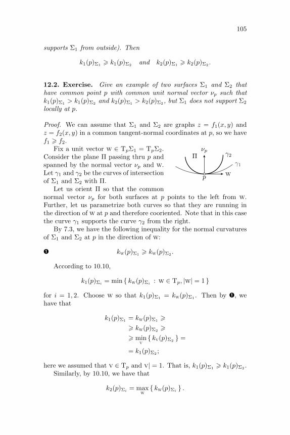
105
supports Σ1 from outside). Then
k1(p)Σ1> k1(p)Σ2
and k2(p)Σ1> k2(p)Σ2
.
12.2. Exercise. Give an example of two surfaces Σ1 and Σ2 thathave common point p with common unit normal vector νp such thatk1(p)Σ1
> k1(p)Σ2and k2(p)Σ1
> k2(p)Σ2, but Σ1 does not support Σ2
locally at p.
Proof. We can assume that Σ1 and Σ2 are graphs z = f1(x, y) andz = f2(x, y) in a common tangent-normal coordinates at p, so we havef1 > f2.
p w
νp
γ1
γ2ΠFix a unit vector w ∈ TpΣ1 = TpΣ2.
Consider the plane Π passing thru p andspanned by the normal vector νp and w.Let γ1 and γ2 be the curves of intersectionof Σ1 and Σ2 with Π.
Let us orient Π so that the commonnormal vector νp for both surfaces at p points to the left from w.Further, let us parametrize both curves so that they are running inthe direction of w at p and therefore cooriented. Note that in this casethe curve γ1 supports the curve γ2 from the right.
By 7.3, we have the following inequality for the normal curvaturesof Σ1 and Σ2 at p in the direction of w:
Ê kw(p)Σ1> kw(p)Σ2
.
According to 10.10,
k1(p)Σi = min kw(p)Σi : w ∈ Tp, |w| = 1
for i = 1, 2. Choose w so that k1(p)Σ1= kw(p)Σ1
. Then by Ê, wehave that
k1(p)Σ1= kw(p)Σ1
>
> kw(p)Σ2>
> minv kv(p)Σ2
=
= k1(p)Σ2 ;
here we assumed that v ∈ Tp and v| = 1. That is, k1(p)Σ1> k1(p)Σ2
.Similarly, by 10.10, we have that
k2(p)Σi = maxw kw(p)Σi .

106 CHAPTER 12. SUPPORTING SURFACES
Let us fix w so that k2(p)Σ2= kw(p)Σ2
. Then
k2(p)Σ2 = kw(p)Σ2 6
6 kw(p)Σ1 6
6 maxv kv(p)Σ1 =
= k2(p)Σ1;
that is, k2(p)Σ1> k2(p)Σ2
.
12.3. Corollary. Let Σ1 and Σ2 be oriented surfaces. Assume Σ1
locally supports Σ2 from inside at the point p. Then
(a) H(p)Σ1> H(p)Σ2
;
(b) If k1(p)Σ2> 0, then K(p)Σ1
> K(p)Σ2.
Proof. Part (a) follows from 12.1 and the definition of mean curvature
H(p)Σi = k1(p)Σi + k2(p)Σi .
(b). Since k2(p)Σi > k1(p)Σi and k1(p)Σ2> 0, we get that all the
principle curvatures k1(p)Σ1 , k1(p)Σ2 , k2(p)Σ1 , and k2(p)Σ2 are non-negative. By 12.1, it implies that
K(p)Σ1= k1(p)Σ1
·k2(p)Σ1>
> k1(p)Σ2·k2(p)Σ2
=
= K(p)Σ2.
12.4. Exercise. Show that any closed surface in a unit ball has apoint with Gauss curvature at least 1.
12.5. Exercise. Show that any closed surface that lies on the distanceat most 1 from a straight line has a point with Gauss curvature atleast 1.
Convex surfaces
A proper surface without boundary that bounds a convex region iscalled convex.
12.6. Exercise. Show that Gauss curvature of any convex smoothsurface is nonnegative at each point.

107
12.7. Exercise. Assume R is a convex body in R3 bounded by asurface with principle curvatures at most 1. Show that R contains aunit ball.
Recall that a region R in the Euclidean space is called strictlyconvex if for any two points x, y ∈ R, any point z between x and ylies in the interior of R.
Clearly any open convex set is strictly convex; the cube (as well asany convex polyhedron) gives an example of a convex set which is notstrictly convex. It is easy to see that a closed convex region is strictlyconvex if and only if its boundary does not contain a line segment.
12.8. Lemma. Let z = f(x, y) be the local description of a smoothsurface Σ in a tangent-normal coordinates at some point p ∈ Σ. As-sume both principle curvatures of Σ are positive at p. Then the func-tion f is strictly convex in a neighborhood of the origin and has a localminimum at the origin.
In particular the tangent plane Tp locally supports Σ from outsideat p.
Proof. Since both principle curvatures are positive, we have that
D2wf(0, 0) = 〈Sp(w),w〉 > 0
for any unit tangent vector w ∈ TpΣ (which is the (x, y)-plane).Since the set of unit vectors is compact, we have that
D2wf(0, 0) > ε
for some fixed ε > 0 and any unit tangent vector w ∈ TpΣ.By continuity of the function (x, y,w) 7→ D2
wf(x, y), we have thatD2
wf(x, y) > 0 if w 6= 0 and (x, y) lies in a neighborhood of the origin.That is, f is a strictly convex function in a neighborhood of the originin the (x, y)-plane.
Finally since ∇f(0, 0) = 0 and f is strictly convex in a neighbor-hood of the origin it has a strict local minimum at the origin.
12.9. Exercise. Let Σ be a smooth surface (without boundary) withpositive Gauss curvature. Show that any connected component of in-tersection of Σ with a plane Π is either a single point or a smoothregular plane that can be parameterized so that it has positive signedcurvature.
The following theorem gives a global description of surfaces withpositive Gauss curvature.

108 CHAPTER 12. SUPPORTING SURFACES
12.10. Theorem. Suppose Σ is a proper smooth surface with positiveGauss curvature. Then Σ bounds a strictly convex region.
Note that in the proof we have to use that surface is a connectedset; otherwise a pair of disjoint spheres which bound two disjoint ballswould give a counterexample.
Proof. Since the Gauss curvature is positive, we can choose unit nor-mal field ν on Σ so that the principle curvatures are positive at anypoint. Denote by R the region bounded by Σ that lies on the side ofν; that is, ν points inside of R at any point of Σ. (The region R existsby 8.1.)
Fix p ∈ Σ; let z = f(x, y) be a local description of Σ in thetangent-normal coordinates at p. By 12.8, f is strictly convex in aneighborhood of the origin. In particular the intersection of a smallball centered at p with the epigraph z > f(x, y) is strictly convex. Inother words, R is locally strictly convex ; that is, for any point p ∈ R,the intersection of R with a small ball centered at p is strictly convex.
Since Σ is connected, so is R; moreover any two points in theinterior of R can be connected by a polygonal line in the interior of R.
x y
y0
z0
z
RΣ
ν
Assume the interior of R is not con-vex; that is, there are points x, y ∈ Rand a point z between x and y that doesnot lie in the interior of R. Consider apolygonal line β from x to y in the in-terior of R. Let y0 be the first point onβ such that the chord [x, y0] touches Σat some point, say z0.
Since R is locally strictly convex,R ∩ B(z0, ε) is strictly convex for all sufficiently small ε > 0.On the other hand z0 lies between two points in the intersection[x, y0] ∩B(z0, ε). Since [x, y0] ⊂ R, we arrived to a contradiction.
Therefore the interior of R is a convex set. Note that the region Ris the closure of its interior, therefore R is convex as well.
Since R is locally strictly convex, its boundary Σ contains no linesegments. Therefore R is strictly convex.
Note that the proof above implies that any connected locally convexregion is convex.
12.11. Exercise. Assume that a closed surface Σ surrounds a unitcircle. Show that Gauss curvature of Σ is at most 1 at some point.
12.12. Exercise. Let Σ be a closed smooth surface of diameter atleast π; that is, there is a pair of points p, q ∈ Σ such that |p− q| > π.Show that Σ has a point with Gauss curvature at most 1.

109
12.13. Theorem. Suppose Σ is a smooth convex surface.(a) If Σ is compact then it is a smooth sphere; that is, Σ admits a
smooth regular parametrization by S2.(b) If Σ is open then there is a coordinate system such that Σ is a
graph z = f(x, y) of a convex function f defined on a convexopen region of the (x, y)-plane.
The following exercises will guide you thru the proof of both partsof the theorem.
ξ
q
RRRRRRRRRRRRRRRRRRRRRRRRRRRRRRRRRRRRRRRRRRRRRRRRRRRRRRRRRRRRRRRRR
ΣS2
p
q
xn
x1
Σ R
u
. ..
12.14. Exercise. Assume a convex compactregion R contains the origin in its interior andbounded by a smooth surface Σ.
(i) Show that any half-line that starts at theorigin intersects Σ at a single point; thatis, there is a positive function ρ : S2 →→ R such that Σ is formed by points q == ρ(ξ)·ξ for ξ ∈ S2.
(ii) Show that ρ : S2 → R is a smooth func-tion.
(iii) Conclude that ξ 7→ ρ(ξ)·ξ is a smoothregular parametrization S2 → Σ.
12.15. Exercise. Assume a strictly convexclosed noncompact region R contains the ori-gin in its interior and bounded by a smoothsurface Σ.
(i) Show that R contains a half-line `.(ii) Show that any line parallel to ` intersects Σ at
most at one point.(iii) Consider (x, y, z)-coordinate system such that
the z-axis points in the direction of `. Showthat projection of Σ to the (x, y) plane is anopen convex set; denote it by Ω.
(iv) Conclude that Σ is a graph z = f(x, y) of aconvex function f defined on Ω.
12.16. Exercise. Show that any open surface Σ with positive Gausscurvature is a topological plane; that is, there is an embedding R2 → R3
with image Σ.Try to show that Σ is a smooth plane; that is, the embedding f can
be made smooth and regular.
12.17. Exercise. Show that any open smooth surface Σ with positiveGauss curvature lies inside of an infinite circular cone.

110 CHAPTER 12. SUPPORTING SURFACES
12.18. Exercise. Suppose Σ is a smooth convex surface. Show that(a) If Σ is closed, then the spherical map ν : Σ → S2 is a bijection.
Conclude that ∫Σ
K = 4·π.
(b) If Σ is open, then the spherical map ν : Σ→ S2 maps Σ ineffec-tively into a subset of a hemisphere. Conclude that∫
Σ
K 6 2·π.
Saddle surfaces
A surface is called saddle if its Gausscurvature at each point is nonpositive;in other words principle curvatures ateach point have opposite signs or one ofthem is zero.
If the Gauss curvature is negativeat each point, then the surface is calledstrictly saddle; equivalently it means that the principle curvatures haveopposite signs at each point. Note that in this case the tangent planedoes not support the surface even locally — moving along the surfacein the principle directions at a given point, one goes above and belowthe tangent plane at this point.
12.19. Exercise. Let f : R→ R be a smooth positive function. Showthat the surface of revolution of the graph y = f(x) around the x-axisis saddle if and only if f is convex; that is, if f ′′(x) > 0 for any x.
A surface Σ is called ruled if for every point p ∈ Σ there is a linesegment `p ⊂ Σp thru p that is infinite or has its endpoint(s) on theboundary line of Σ.
12.20. Exercise. Show that any ruled surface Σ is saddle.
12.21. Exercise. Suppose Σ is an open saddle surface. Show thatfor any point p ∈ Σ there is a curve γ : [0,∞) → Σ that starts at pand monotonically escapes to infinity; that is, the function t 7→ |γ(t)|is increasing and |γ(t)| → ∞ as t→∞.
A tangent direction on a smooth surface with vanishing normalcurvature is called asymptotic. A smooth regular curve that alwaysruns in an asymptotic direction is called an asymptotic line.

111
12.22. Advanced exercise. Let γ be a closed smooth asymptoticline in a graph z = f(x, y) of a smooth function f . Assume Σ isstrictly saddle in a neighborhood of γ. Show that the projection of γto the (x, y)-plane cannot be star-shaped.
Hats
Note that a closed surface cannot be saddle. Indeed consider a smallestsphere that contains a closed surface Σ inside; it supports Σ at somepoint p and at this point the principle curvature must have the samesign. The following more general statement is proved using the sameidea.
12.23. Lemma. Assume Σ is a compact saddle surface and its bound-ary line lies in a convex closed region R. Then whole surface Σ liesin R.
pq
RRRRRRRRRRRRRRRRRRRRRRRRRRRRRRRRRRRRRRRRRRRRRRRRRRRRRRRRRRRRRRRRR
Π
Σ0
Σ∂Σ∂Σ∂Σ∂Σ∂Σ∂Σ∂Σ∂Σ∂Σ∂Σ∂Σ∂Σ∂Σ∂Σ∂Σ∂Σ∂Σ∂Σ∂Σ∂Σ∂Σ∂Σ∂Σ∂Σ∂Σ∂Σ∂Σ∂Σ∂Σ∂Σ∂Σ∂Σ∂Σ∂Σ∂Σ∂Σ∂Σ∂Σ∂Σ∂Σ∂Σ∂Σ∂Σ∂Σ∂Σ∂Σ∂Σ∂Σ∂Σ∂Σ∂Σ∂Σ∂Σ∂Σ∂Σ∂Σ∂Σ∂Σ∂Σ∂Σ∂Σ∂Σ∂Σ∂Σ∂Σ
Proof. Arguing by contradiction,assume there is point p ∈ Σ thatdoes not lie in R. Let Π be a planethat separates p from R; it existsby E.4. Denote by Σ′ the part ofΣ that lies with p on the same sidefrom Π.
Since Σ is compact, it is sur-rounded by a sphere; let σ bethe circle of intersection of thissphere and Π. Consider the small-est spherical dome Σ0 with bound-ary σ that surrounds Σ′.
Note that Σ0 supports Σ at some point q. Without loss of gener-ality we may assume that Σ0 and Σ are cooriented at q and Σ0 haspositive principle curvatures. In this case Σ0 supports ∆ from outside.By we have 12.3, K(q)Σ > K(q)Σ0
> 0 — a contradiction.
Note that if we assume that Σ is strictly saddle, then we couldarrive to a contradiction by taking a point q ∈ Σ on the maximaldistance from R.
12.24. Exercise. Let ∆ be a compact smooth regular saddle sur-face with boundary and p ∈ ∆. Suppose that the boundary line of ∆lies in the unit sphere centered at p. Show that if ∆ is a disc, thenlength(∂∆) > 2·π.
Show that the statement does not hold without assuming that ∆ isa disc.

112 CHAPTER 12. SUPPORTING SURFACES
If ∆ is as in the exercise, then in fact area ∆ > π. The proof of thisstatement can be obtained by applying the so called coarea fromulatogether with the inequality in the exercise.
12.25. Exercise. Show that an open saddle surface cannot lie insideof an infinite circular cone.
A disc ∆ in a surface Σ is called a hat of Σ if its boundary line ∂∆lies in a plane Π and the remaining points of ∆ lie on one side of Π.
12.26. Proposition. A smooth surface Σ is saddle if and only if ithas no hats.
Note that a saddle surface can contain a closed plane curve. Forexample the hyperboloid x2 + y2 − z2 = 1 contains the unit circle inthe (x, y)-plane. However, according to the proposition (as well as thelemma), a plane curve cannot bound a disc (as well any compact set)in a saddle surface.
Proof. Since plane is convex, the “only if” part follows from 12.23; itremains to prove the “if” part.
Assume Σ is not saddle; that is, it has a point p with strictly pos-itive Gauss curvature; or equivalently, the principle curvatures k1(p)and k2(p) have the same sign.
Let z = f(x, y) be a graph representation of Σ in the tangent-normal coordinates at p. By 12.8, f is convex in a small neighborhoodof (0, 0). In particular the set Fε defined by the inequality f(x, y) 6 εis convex for sufficiently small ε > 0; in particular, it is a topologicaldisc. Note that (x, y) 7→ (x, y, f(x, y)) is a homeomorphism from Fεto
∆ε =
(x, y, f(x, y)) ∈ R3 : f(x, y) 6 ε
;
so ∆ε is a topological disc for any sufficiently small ε > 0. Note thatthe boundary line of ∆ε lies on the plane z = ε and whole disc liesbelow it; that is, ∆ε is a hat of Σ.
The following exercise shows that ∆ε is in fact a smooth disc. Itcan be used to prove slightly stronger version of 12.26; namely one canthe disc in the definition of hat is a smooth disc.
12.27. Exercise. Let f : R2 → R be a smooth strictly convex func-tion with minimum at the origin. Show that the set Fε defined by theinequality f(x, y) 6 ε is a smooth disc for any ε > 0; that is, there isa diffeomorphism D→ Fε, where D =
(x, y) ∈ R2 : x2 + y2 6 1
is
the unit disc.
12.28. Exercise. Let T : R3 → R3 be a linear transformation; thatis, T is an invertable map R3 → R3 that sends any plane to a plane.

113
Show that for any saddle surface Σ the image T (Σ) is also a saddlesurface.
Saddle graphs
The following theorem was proved by Sergei Bernstein [4].
12.29. Theorem. Let f : R2 → R be a smooth function. Assume itsgraph z = f(x, y) is a strictly saddle surface in R3. Then f is notbounded; that is, there is no constant C such that |f(x, y)| 6 C forany (x, y) ∈ R2.
The theorem states that a saddle graph cannot lie between parallelhorizontal planes; applying 12.28 we get that saddle graphs cannotlie between parallel planes, not necessarily horizontal. The followingexercise shows that the theorem does not hold for saddle surfaces whichare not graphs.
12.30. Exercise. Construct an open strictly saddle surface that liesbetween parallel planes.
Since exp(x − y2) > 0, the following exercise shows that thereare strictly saddle graphs with functions bounded on one side; that is,both (upper and lower) bounds are needed in the proof of Bernshtein’stheorem.
12.31. Exercise. Show that the graph z = exp(x − y2) is strictlysaddle.
Note that according to 12.23, there are no proper saddle surfacesin a parallelepiped that boundary line lies on one of its faces. Thefollowing lemma gives an analogous statement for a parallelepiped withan infinite side.
12.32. Lemma. There is no proper strictly saddle smooth surfacethat lies on bounded distance from a line and has its boundary line ina plane.
Proof. Note that in a suitable coordinate system, the statement canbe reformulated the following way: There is no proper strictly saddlesmooth surface with the boundary line in the (x, y)-plane that lies in aregion of the following form:
R =
(x, y, z) ∈ R3 : 0 6 z 6 r, 0 6 y 6 r.
Let us prove this statement.

114 CHAPTER 12. SUPPORTING SURFACES
Assume contrary, let Σ be such a surface. Consider the projectionΣ of Σ to the (x, z)-plane. It lies in the upper half-plane and belowthe line z = r.
Consider the open upper half-plane H =
(x, z) ∈ R2 : z > 0
.
Let Θ be the connected component of the complement H\Σ that con-tains all the points above the line z = r.
Note that Θ is convex. If not, then there is a line segment [pq] forsome p, q ∈ Θ that cuts from Σ a compact piece. Consider the plane
p qΘ
ΣΣΣΣΣΣΣΣΣΣΣΣΣΣΣΣΣΣΣΣΣΣΣΣΣΣΣΣΣΣΣΣΣΣΣΣΣΣΣΣΣΣΣΣΣΣΣΣΣΣΣΣΣΣΣΣΣΣΣΣΣΣΣΣΣ
z = r
z = 0
Π thru [pq] that is perpendicular to the (x, z)-plane. Note that Π cutsfrom Σ a compact region ∆. By general position argument (see 9.10)we can assume that ∆ is a compact surface with boundary line in Πand the remaining part of ∆ lies on one side from Π. Since the planeΠ is convex, this statement contradicts 12.23.
Summarizing, Θ is an open convex set of H that contains all pointsabove z = r. By convexity, together with any point w, the set Θcontains all points on the half-lines that point up from it. Whence itcontain all points with z-coordinate larger than the z-coordinate of w.Since Θ is open it can be described by inequality z > r0. It follows that
Θ
ΣΣΣΣΣΣΣΣΣΣΣΣΣΣΣΣΣΣΣΣΣΣΣΣΣΣΣΣΣΣΣΣΣΣΣΣΣΣΣΣΣΣΣΣΣΣΣΣΣΣΣΣΣΣΣΣΣΣΣΣΣΣΣΣΣ
z = r
z = r0w
z = 0
the plane z = r0 supports Σ at some point (in fact at many points).By 12.1, the latter is impossible — a contradiction.
Proof of 12.29. Denote by Σ the graph z = f(x, y). Assume contrary;that is, Σ lies between two planes z = ±C.
Note that the function f cannot be constant. It follows that thetangent plane Tp at some point p ∈ Σ is not horizontal.
Denote by Σ+ the part of Σ that lies above Tp. Note that ithas at least two connected components which are approaching p from

115
both sides in the principle direction with positive principle curvature.Indeed if there would be a curve that runs in Σ+ and approaches pfrom both sides, then it would cut a disc from Σ with boundary lineabove Tp and some points below it; the latter contradicts 12.23.
h = −Ch = −Ch = −Ch = −Ch = −Ch = −Ch = −Ch = −Ch = −Ch = −Ch = −Ch = −Ch = −Ch = −Ch = −Ch = −Ch = −Ch = −Ch = −Ch = −Ch = −Ch = −Ch = −Ch = −Ch = −Ch = −Ch = −Ch = −Ch = −Ch = −Ch = −Ch = −Ch = −Ch = −Ch = −Ch = −Ch = −Ch = −Ch = −Ch = −Ch = −Ch = −Ch = −Ch = −Ch = −Ch = −Ch = −Ch = −Ch = −Ch = −Ch = −Ch = −Ch = −Ch = −Ch = −Ch = −Ch = −Ch = −Ch = −Ch = −Ch = −Ch = −Ch = −Ch = −Ch = −C
h = CΣ+
0Σ+0Σ+0Σ+0Σ+0Σ+0Σ+0Σ+0Σ+0Σ+0Σ+0Σ+0Σ+0Σ+0Σ+0Σ+0Σ+0Σ+0Σ+0Σ+0Σ+0Σ+0Σ+0Σ+0Σ+0Σ+0Σ+0Σ+0Σ+0Σ+0Σ+0Σ+0Σ+0Σ+0Σ+0Σ+0Σ+0Σ+0Σ+0Σ+0Σ+0Σ+0Σ+0Σ+0Σ+0Σ+0Σ+0Σ+0Σ+0Σ+0Σ+0Σ+0Σ+0Σ+0Σ+0Σ+0Σ+0Σ+0Σ+0Σ+0Σ+0Σ+0Σ+0Σ+0Σ+0
Σ+1Σ+1Σ+1Σ+1Σ+1Σ+1Σ+1Σ+1Σ+1Σ+1Σ+1Σ+1Σ+1Σ+1Σ+1Σ+1Σ+1Σ+1Σ+1Σ+1Σ+1Σ+1Σ+1Σ+1Σ+1Σ+1Σ+1Σ+1Σ+1Σ+1Σ+1Σ+1Σ+1Σ+1Σ+1Σ+1Σ+1Σ+1Σ+1Σ+1Σ+1Σ+1Σ+1Σ+1Σ+1Σ+1Σ+1Σ+1Σ+1Σ+1Σ+1Σ+1Σ+1Σ+1Σ+1Σ+1Σ+1Σ+1Σ+1Σ+1Σ+1Σ+1Σ+1Σ+1Σ+1
p
R−R−R−R−R−R−R−R−R−R−R−R−R−R−R−R−R−R−R−R−R−R−R−R−R−R−R−R−R−R−R−R−R−R−R−R−R−R−R−R−R−R−R−R−R−R−R−R−R−R−R−R−R−R−R−R−R−R−R−R−R−R−R−R−R−
R0R0R0R0R0R0R0R0R0R0R0R0R0R0R0R0R0R0R0R0R0R0R0R0R0R0R0R0R0R0R0R0R0R0R0R0R0R0R0R0R0R0R0R0R0R0R0R0R0R0R0R0R0R0R0R0R0R0R0R0R0R0R0R0R0
R+R+R+R+R+R+R+R+R+R+R+R+R+R+R+R+R+R+R+R+R+R+R+R+R+R+R+R+R+R+R+R+R+R+R+R+R+R+R+R+R+R+R+R+R+R+R+R+R+R+R+R+R+R+R+R+R+R+R+R+R+R+R+R+R+
The surface Σ seeing from above.
Summarizing, Σ+ has at least two connected components, denotethem by Σ+
0 and Σ+1 . Let z = h(x, y) = a·x+ b·y + c be the equation
of Tp. Note that Σ+ contains all points in the region
R− = (x, y, f(x, y)) ∈ Σ : h(x, y) < −C
which is a connected set and no points in
R+ = (x, y, f(x, y)) ∈ Σ : h(x, y) > C
Whence one of the connected components, say Σ+0 , lies in
R0 = (x, y, f(x, y)) ∈ Σ : |h(x, y)| 6 C .
This set lies on a bounded distance from the line of intersection of Tpwith the (x, y)-plane.
Moving the plane Tp slightly upward, we can cut from Σ+0 a proper
surface with boundary line lying in this plane (see 9.10). The obtainedsurface is still on a bounded distance to a line which is impossible by12.32.
The following exercise gives a condition that guarantees that a sad-dle surface is a graph; it can be used in combination with Bernshtein’stheorem.
12.33. Advanced exercise. Let Σ be a smooth saddle disk in R3.Assume that the orthogonal projection to the (x, y)-plane maps theboundary line of Σ injectively to a convex closed curve. Show that theorthogonal projection to the (x, y)-plane is injective on Σ.
In particular, Σ is the graph z = f(x, y) of a function f defined ona convex figure in the (x, y)-plane.

116 CHAPTER 12. SUPPORTING SURFACES
Remarks
Note that Bernstein’s theorem and the lemma in its proof do not holdfor nonstrictly saddle surfaces; counterexamples can be found amonginfinite cylinders over smooth regular curves. In fact it can be shownthat these are the only counterexamples; a proof is based on the sameidea, but more technical.
By 12.26, saddle surfaces can be defined as smooth surfaces withouthats. This definition can be used for arbitrary surfaces, not necessar-ily smooth. Some results, for example Bernshtein’s characterizationof saddle graphs can be extended to generalized saddle surfaces, butthis class of surfaces is far from being understood. Some nontrivialproperties were proved by Samuil Shefel [33]; see also [1, Capter 4].

Chapter 13
Shortest paths
Shortest paths
Let p and q be two points on a surface Σ. Recall that |p− q|Σ denotesthe induced length distance from p to q; that is, the exact lower boundon lengths of paths in Σ from p to q.
Note that if Σ is smooth, then any two points in Σ can be joinedby a piecewise smooth path. Since any such path is rectifiable, thevalue |p− q|Σ is finite for any pair p, q ∈ Σ.
A path γ from p to q in Σ that minimizes the length is called ashortest path from p to q.
The image of a shortest path between p and q in Σ is usuallydenoted by [p, q]Σ. In general there might be no shortest path betweentwo given points on the surface and it might be many of them; this isshown in the following two examples.
Usually, if we write [p, q]Σ, then we assume that a shortest pathexists and we made a choice of one of them.
pq
sε
Nonuniqueness. There are plenty of shortestpaths between the poles on the sphere — eachmeridian is a shortest path.
Nonexistence. Let Σ be the (x, y)-plane withremoved origin. Consider two points p = (1, 0, 0)and q = (−1, 0, 0) in Σ.
Note that |p − q|Σ = 2. Indeed, given ε > 0,consider the point sε = (0, ε, 0). Observe thatthe polygonal path psεq lies in Σ and its length2·√
1 + ε2 approaches 2 as ε→ 0. It follows that
117

118 CHAPTER 13. SHORTEST PATHS
|p − q|Σ 6 2. On the other hand |p − q|Σ > |p − q|R3 = 2; therefore|p− q|Σ = 2.
It follows that a shortest path from p to q, if it exists, must havelength 2. By triangle inequality any curve of length 2 from p to q mustrun along the line segment [p, q]; in particular it must pass thru theorigin. Since the origin does not lie in Σ, there is no shortest from pto q in Σ
13.1. Proposition. Any two points in a proper smooth surface canbe joined by a shortest path.
Proof. Fix a proper smooth surface Σ with two points p and q. Set` = |p− q|Σ.
By the definition of induced length metric, there is a sequence ofpaths γn from p to q in Σ such that
length γn → ` as n→∞.
Without loss of generality, we may assume that length γn < ` + 1for any n and each γn is parameterized proportional to its arc-length.In particular each path γn : [0, 1]→ Σ is (`+ 1)-Lipschitz; that is,
|γ(t0)− γ(t1)| 6 (`+ 1)·|t0 − t1|
for any t0, t1 ∈ [0, 1].Note that the image of γn lies in the closed ball B[p, ` + 1] for
any n. It follows that the coordinate functions of γn are uniformlyequicontinuous and uniformly bounded. By C.3, we can pass to aconverging subsequence of γn; denote by γ∞ : [0, 1]→ R3 its limit.
As a limit of uniformly continuous sequence, γ∞ is continuous; thatis, γ∞ is a path. Evidently γ∞ runs from p to q; in particular
length γ∞ > `.
Since Σ is a closed set, γ∞ lies in Σ. Finally, by 3.15,
length γ∞ 6 `.
That is, γ∞ = ` or, equivalently, γ∞ is a shortest path from p to q.
Closest point projection
13.2. Lemma. Let R be a closed convex set in R3. Then for everypoint p ∈ R3 there is a unique point p ∈ R that minimizes the distance|p− x| among all points x ∈ R.

119
Moreover the map p 7→ p is short; that is,
Ê |p− q| > |p− q|
for any pair of points p, q ∈ R3.
The map p 7→ p is called the closest point projection; it maps theEuclidean space to R. Note that if p ∈ R, then p = p.
Proof. Fix a point p and set
` = inf |p− x| : x ∈ R .
Choose a sequence xn ∈ R such that |p− xn| → ` as n→∞.
p
pp′ m
Without loss of generality, we can assume that allthe points xn lie in a ball of radius ` + 1 centeredat p. Therefore we can pass to a partial limit p of xn;that is, p is a limit of a subsequence of xn. Since Ris closed, p ∈ R. By construction
|p− p| = limn→∞
|p− xn| =
= `.
Hence the existence follows.Assume there are two distinct points p, p′ ∈ R
that minimize the distance to p. Since R is convex, their midpointm = 1
2 ·(p + p′) lies in R. Note that |p − p| = |p − p′| = `; that is,4ppp′ is isosceles and therefore 4ppm is right with the right angleat m. Since a leg of a right triangle is shorter than its hypotenuse, wehave |p−m| < ` — a contradiction.
It remains to prove inequality Ê.
p q
ppppppppppppppppppppppppppppppppppppppppppppppppppppppppppppppppp qqqqqqqqqqqqqqqqqqqqqqqqqqqqqqqqqqqqqqqqqqqqqqqqqqqqqqqqqqqqqqqqqRRRRRRRRRRRRRRRRRRRRRRRRRRRRRRRRRRRRRRRRRRRRRRRRRRRRRRRRRRRRRRRRR
We can assume that p 6= q, otherwisethere is nothing to prove. Note that if p 6= p(that is, if p /∈ R), then ∠ppq is right orobtuse. Otherwise there would be a point xon the line segment [q, p] that is closer to pthan p. Since R is convex, the line segment[q, p] and therefore x lie in R. Hence p isnot closest to p — a contradiction.
The same way we can show that if q 6= q,then ∠qqp is right or obtuse.
We have to consider the following 4 cases: (1) p 6= p and q 6= q,(2) p = p and q 6= q, (3) p 6= p and q = q, (4) p = p and q = q. Inall these cases the obtained angle estimates imply that the orthogonal
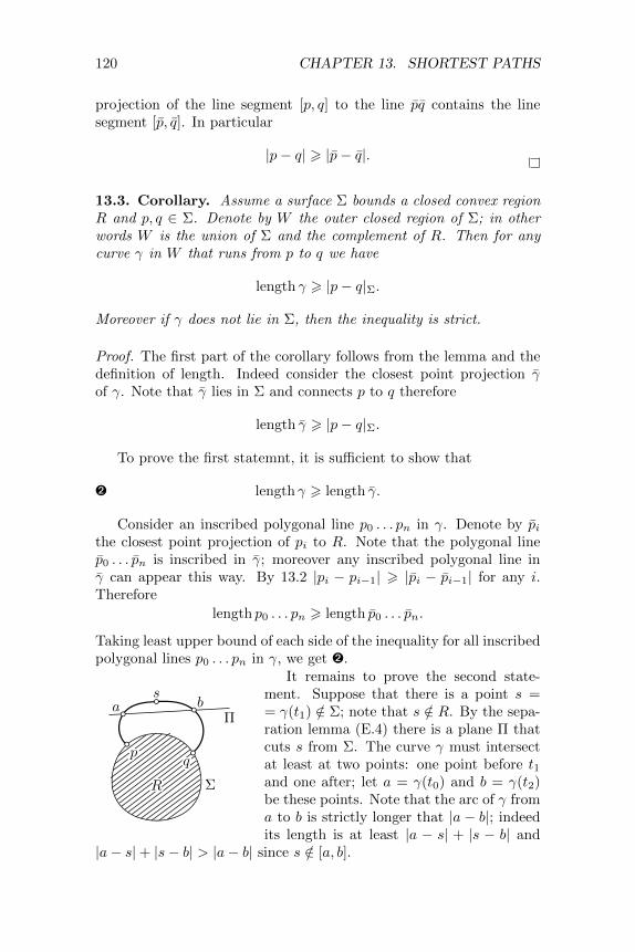
120 CHAPTER 13. SHORTEST PATHS
projection of the line segment [p, q] to the line pq contains the linesegment [p, q]. In particular
|p− q| > |p− q|.
13.3. Corollary. Assume a surface Σ bounds a closed convex regionR and p, q ∈ Σ. Denote by W the outer closed region of Σ; in otherwords W is the union of Σ and the complement of R. Then for anycurve γ in W that runs from p to q we have
length γ > |p− q|Σ.
Moreover if γ does not lie in Σ, then the inequality is strict.
Proof. The first part of the corollary follows from the lemma and thedefinition of length. Indeed consider the closest point projection γof γ. Note that γ lies in Σ and connects p to q therefore
length γ > |p− q|Σ.
To prove the first statemnt, it is sufficient to show that
Ë length γ > length γ.
Consider an inscribed polygonal line p0 . . . pn in γ. Denote by pithe closest point projection of pi to R. Note that the polygonal linep0 . . . pn is inscribed in γ; moreover any inscribed polygonal line inγ can appear this way. By 13.2 |pi − pi−1| > |pi − pi−1| for any i.Therefore
length p0 . . . pn > length p0 . . . pn.
Taking least upper bound of each side of the inequality for all inscribedpolygonal lines p0 . . . pn in γ, we get Ë.
ppppppppppppppppppppppppppppppppppppppppppppppppppppppppppppppppp qqqqqqqqqqqqqqqqqqqqqqqqqqqqqqqqqqqqqqqqqqqqqqqqqqqqqqqqqqqqqqqqq
a bs
Σ
Π
RRRRRRRRRRRRRRRRRRRRRRRRRRRRRRRRRRRRRRRRRRRRRRRRRRRRRRRRRRRRRRRRR
It remains to prove the second state-ment. Suppose that there is a point s == γ(t1) /∈ Σ; note that s /∈ R. By the sepa-ration lemma (E.4) there is a plane Π thatcuts s from Σ. The curve γ must intersectat least at two points: one point before t1and one after; let a = γ(t0) and b = γ(t2)be these points. Note that the arc of γ froma to b is strictly longer that |a − b|; indeedits length is at least |a − s| + |s − b| and
|a− s|+ |s− b| > |a− b| since s /∈ [a, b].

121
Remove from γ the arc from a to b and glue in the line segment[a, b]; denote the obtained curve by γ1. From above, we have that
length γ > length γ1
Note that γ1 runs in W . Therefore by the first part of corollary, wehave
length γ1 > |p− q|Σ.
Whence the second statement follows.
∆
Σ
Π
13.4. Exercise. Suppose Σ is a closed smoothsurface that bounds a convex region R in R3 andΠ is a plane that cuts a hat ∆ from Σ. Assumethat the reflection of the interior of ∆ with respectto Π lies in the interior of R. Show that ∆ isconvex with respect to the intrinsic metric of Σ;that is, if both ends of a shortest path in Σ lie in∆, then the entire geodesic lies in ∆.
Let us define the intrinsic diameter of a closed surface Σ as theexact upper bound on the lengths of shortest paths in the surface.
13.5. Exercise. Assume that a closed smooth surface Σ with positiveGauss curvature lies in a unit ball.
(a) Show that the intrinsic diameter of Σ cannot exceed π.(b) Show that the area of Σ cannot exceed 4·π.

Chapter 14
Geodesics
Definitions
A smooth curve γ on a smooth surface Σ is called geodesic if its accel-eration γ′′(t) is perpendicular to the tangent plane Tγ(t) at any t.
14.1. Exercise. Assume that a smooth surface Σ is mirror symmet-ric with respect to a plane Π. Suppose that Σ and Π intersect along asmooth regular curve γ. Show that γ is a geodesic of Σ.
14.2. Exercise. Show that the helix
γ(t) = (cos t, sin t, a·t)
is a geodesic on the cylindrical surface described by the equation x2 ++ y2 = 1.
Recall that asymptotic line is defined on page 110.
14.3. Exercise. Suppose that a curve γ is a geodesic and, at thesame time, is an asymptotic line on a smooth surface Σ. Show that γis a line segment.
Physically, geodesics can be understood as the trajectories of aparticle that slides on Σ without friction. In this case the force thatkeeps the particle on Σ must be perpendicular to Σ. Therefore, bythe second Newton’s laws of motion, we get that the acceleration γ′′
is perpendicular to Tγ(t).The following lemma and proposition can be also interpreted phys-
ically; lemma follow from the conservation of energy and the proposi-tion gives smooth dependence of trajectory of a particle depending onits initial position and velocity.
122

123
14.4. Lemma. Any geodesic γ has constant speed; that is, |γ′(t)| isconstant.
Proof. Since γ′(t) is a tangent vector at γ(t), we have that γ′′(t) ⊥⊥ γ′(t), or equivalently 〈γ′′, γ′〉 = 0 for any t. Whence
〈γ′, γ′〉′ = 2·〈γ′′, γ′〉 =
= 0.
That is, |γ′(t)|2 = 〈γ′(t), γ′(t)〉 is constant.
14.5. Proposition. Let Σ be a smooth surface without boundary.Given a tangent vector v to Σ at a point p there is a unique geodesicγ : I → Σ defined on a maximal open interval I 3 0 that starts at pwith velocity vector v; that is, γ(0) = p and γ′(0) = v.
Moreover
(a) the map (p,v, t) 7→ γ(t) is smooth in its domain of definition.
(b) if Σ is proper, then I = R; that is, the maximal interval is wholereal line.
This proposition follows from the theorem on existence and unique-ness of the initial value problem (B.1).
14.6. Lemma. A smooth curve t 7→ γ(t) = (x(t), y(t), z(t)) is ageodesic in a graph z = f(x, y) if and only if z(t) = f(x(t), y(t)) forany t and the functions t 7→ x(t) and t 7→ y(t) satisfy a differentialequation
x′′ = g(x, y, x′, y′),
y′′ = h(x, y, x′, y′),
where the functions g and h are smooth functions of four variables thatdetermined by f .
The proof of the lemma is done by means of direct calculations.
Proof. In the following calculations, we often omit the arguments —we may write x instead of x(t) and f instead of f(x, y) or f(x(t), y(t))and so on.
First let us calulate z′′(t) in terms of f , x(t), and y(t).
Ê
z′′(t) = f(x(t), y(t))′′ =
=(∂f∂x ·x
′ + ∂f∂y ·y
′)′
=
= ∂2f∂x2 ·(x′)2 + ∂f
∂x ·x′′ + ∂2f
∂y2 ·(y′)2 + ∂f
∂y ·y′′.

124 CHAPTER 14. GEODESICS
Now observe that the equation
Ë γ′′(t) ⊥ Tγ(t)
means that γ′′ is perpendicular to two basis vectors in Tγ(t). Thereforethe vector equation Ë can be rewritten as the following system of tworeal equations
〈γ′′(t), ∂s∂x 〉 = 0,
〈γ′′(t), ∂s∂y 〉 = 0,
where s(x, y) := (x, y, f(x, y)), x = x(t), and y = y(t).Observe that ∂s
∂x = (1, 0, ∂f∂x ) and ∂s∂y = (0, 1, ∂f∂y ). Since γ′′ =
= (x′′, y′′, z′′), we can rewrite the system the following way.x′′ + ∂f
∂x ·z′′ = 0,
y′′ + ∂f∂y ·z
′′ = 0,
It remains use expression Î for z′′, combine like terms and simplify.
Proof of 14.5. Let z = f(x, y) be a description of Σ in a tangent-normal coordinates at p. By Lemma 14.6 the condition γ′′(t) ⊥ Tγ(t)
can be written as a second order differential equation. Applying theexistence and uniqueness of the initial value problem (B.1) we getexistence and uniqueness of geodesic γ in a in a small interval (−ε, ε)for some ε > 0.
Let us extend γ to a maximal open interval I. Suppose there isanother geodesic γ1 with the same initial data that is defined on amaximal open interval I1. Suppose γ1 splits from γ at some timet0 > 0; that is, γ1 coincides with γ on the interval [0, t0), but theyare different on the interval [0, t0 + ε) for any ε > 0. By continuityγ1(t0) = γ(t0) and γ′(t0) = γ′(t0). Therefore by the above argumentγ1 coinsides with γ in a small neighborhood of t0 — a contradiction.
The case t0 < 0 can be proved along the same lines. It follows thatγ1 coincides with γ.
Part ((a)) follows since the solution of the initial value problemdepends smoothly on the initial data (B.1).
Suppose ((b)) does not hold; that is, the maximal interval I is aproper subset of the real line R. Without loss of generality we mayassume that b = sup I <∞.
By 14.4 |γ′| is constant, in particular t 7→ γ(t) is a uniformly con-tinuous function. Therefore the limit
q = limt→b
γ(t)

125
is defined. Since Σ is a proper surface, q ∈ Σ.Applying the argument above in a tangent-normal coordinates at
q shows that γ can be extended as a geodesic behind q. Therefore I isnot a maximal interval — a contradiction.
14.7. Exercise. Let γ be a smooth regular curve in a smooth sur-face Σ. Show that γ is a geodesic if and only if it has constant speedand vanishing geodesic curvature.
Exponential map
Let Σ be smooth regular surface and p ∈ Σ. Given a tangent vectorv ∈ Tp consider a geodesic γv in Σ that runs from p with the initialvelocity v; that is, γ(0) = p and γ′(0) = v.
The point q = γv(1) is called exponential map of v, or brieflyq = expp v. (There is a reason to call this map exponential, but it willtake us too far from the subject.) By 14.5, the map expp : Tp → Σ issmooth and defined in a neighborhood of zero in Tp; moreover, if Σ isproper, then expp is defined on the whole space Tp.
The exponential map expp is defined on the tangent plane Tp whichis a smooth surfaces and its target is another smooth surface Σ. Ob-serve that one can identify the plane plane Tp with its tangent planeT0Tp so the linearization L0 expp is maps Tp to itself.
14.8. Observation. The linearization L0(expp) : Tp → Tp is theidentity map.
Proof. Let z = f(x, y) be a local graph representation of Σ in thetangent-normal coordinates at p, so the tangent plane Tp is the (x, y)-plane.
Let γx and γy be the geodesics starting from p in the directionsv = (1, 0, 0) and w = (0, 1, 0) correspondingly; that is γx(0) = γy(0) =(0, 0, 0), γ′x(0) = v, and γ′y(0) = w.
By the definition of linearization we have that L0(expp)(v) = vand L0(expp)(w) = w. That is, L0(expp) does not move a basis ofTp. Since the linearization L0(expp) is a linear map, it has to beidentity.
Applying the observation together with the inverse function theo-rem (A.1), we get the following statement.
14.9. Proposition. Let Σ be smooth surface and p ∈ Σ. Then theexponential map expp : Tp → Σ is a smooth regular parametrizationof a neighborhood of p in Σ by a neighborhood of 0 in the tangentplane Tp.

126 CHAPTER 14. GEODESICS
Moreover for any p ∈ Σ there is ε > 0 such that for any x ∈ Σsuch that |x − p|Σ < ε the map expx : Tx → Σ is a smooth regularparametrization of the ε-neighborhood of x in Σ by the ε-neighborhoodof zero in the tangent plane Tx.
Polar coordinates
Fix polar coordinates (θ, r) on tangent plane of Σ at p. If v ∈ Tp hascoordinates (θ, r), then we say that q = expp v be the point in Σ withthe polar coordinates (θ, r) with center at p, or briefly q = wp(r, θ).Note that according to Proposition 14.9 polar coordinates behave usualway in a neighborhood of the point in p; that is, there is r0 > such thatif r1, r2 < r0 then wp(r1, θ1) = wp(r2, θ2) if and only if r1 = r2 = 0 orr1 = r2 and θ1 = θ2 + 2·n·π for an integer n.
14.10. Lemma. Let wp(θ, r) describes polar coordinates in a neing-borhood of point p of smooth surface Σ. Then
∂wp∂θ ⊥
∂wp∂r
for any r and θ.
Proof. Note that by the definition of exponential map, for a fixed θ,the curve γθ(t) = w(θ, t) is a unit-speed geodesic that starts at p; inparticular we have the following two identities:
(i) Since the geodesic has unit speed we have | ∂∂rwp| = |γ′θ(r)| = 1.
In particular,∂∂θ 〈
∂wp∂r ,
∂wp∂r 〉 = 0
(ii) Since∂2wp∂r2 = γ′′θ (r) ⊥ Tγθ(r), we have
〈∂2wp∂r2 ,
∂wp∂θ 〉 = 0
Therefore
∂∂r 〈
∂wp∂θ ,
∂wp∂r 〉 = 〈∂
2wp∂θ∂r ,
∂wp∂r 〉+ 〈∂wp∂θ ,
∂2wp∂r2 〉 =
= 12 ·
∂∂θ 〈
∂wp∂r ,
∂wp∂r 〉 =
= 0
That is 〈∂wp∂θ ,∂wp∂r 〉 does not depend on r.
Note that wp(θ, 0) = p for any θ. Therefore∂wp∂θ = 0 and in
particular〈∂wp∂θ ,
∂wp∂r 〉 = 0

127
if r = 0. Since 〈∂wp∂θ ,∂wp∂r 〉 does not depend on r, we get
〈∂wp∂θ ,∂wp∂r 〉 = 0
everywhere. Whence the statement follows.
Shortest paths are geodesics
The following proposition provides the first connection between intrin-sic geometry of the surface and its extrinsic geometry. This connectionwill be important later; in particular it plays the key role in the proofof the so-called Gauss remarkable theorem.
A property is called intrinsic if it is defined in terms of measuringthings inside the surface, for example length of curves or angles be-tween the curves that lie in the surface. Otherwise, if a definition ofproperty use ambient space, then it is called extrinsic.
For instance, a shortest path is an object of intrinsic geometry ofa surface, while definition of geodesic is not intrinsic — it requiresacceleration which needs the ambient space. Note that there is asmooth bijection between the cylinder z = x2 and the plane z = 0that preserves the lengths of all curves; in other words the cylindercan be unfolded on the plane. Such a bijection sends geodesics in thecylinder to geodesics on the plane and the other way around; howevera geodesic on the cylinder might have nonvanishing second derivativewhile geodesics on the plane are straight lines with vanishing secondderivative.
14.11. Proposition. Let Σ be a smooth regular surface. Then anyshortest path γ in Σ parameterized proportional to its arc-length is ageodesic in Σ. In particular γ is a smooth curve.
A partial converse to the first statement also holds: a sufficientlyshort arc of any geodesic is a shortest path. More precisely, any pointp in Σ has a neighborhood U such that any geodesic that lies completelyin U is a shortest path.
A geodesic might not form a shortest path, but if this is the case,then it is called minimizing geodesic. Note that according to the claim,any shortest path is a reparametrization of a minimizing geodesic.
A rigorous proof will be given in the next sections. The follow-ing informal physical explanation might be sufficiently convincing. Infact, if one assumes that γ is smooth, then it is easy to convert thisexplanation into a rigorous proof.
Informal explanation. Let us think about a shortest path γ as ofstable position of a stretched elastic thread that is forced to lie on a

128 CHAPTER 14. GEODESICS
frictionless surface. Since it is frictionless, the force density N(t) thatkeeps the geodesic γ in the surface must be proportional to the normalvector to the surface at γ(t).
The tension in the thread has to be the same at all points (otherwisethe thread would move back or forth and it would not be stable).Denote the tension by T .
We can assume that γ has unit speed; in this case the net forcefrom tension to the arc γ[t0,t1] is T ·(γ′(t1)− γ′(t0). Hence the densityof net force from tension at t0 is
F (t0) = limt1→t0
T · γ′(t1)− γ′(t0)
t1 − t0=
= T ·γ′′(t0).
According to the second Newton’s law of motion, we have
F (t) +N(t) = 0;
which implies that γ′′(t) ⊥ Tγ(t)Σ.
Note that according to the proposition above, any shortest pathparameterized by its arc-length is a smooth curve. This observationshould help to solve in the following two exercises.
14.12. Exercise. Show that two shortest paths can cross each otherat most once. More precisely, if two shortest paths have two distinctcommon points p and q, then either these points are the ends of bothshortest paths or both shortest paths contain an arc from p to q.
Show by example that nonoverlapping geodesics can cross each otheran arbitrary number of times.
14.13. Exercise. Assume that a smooth regular surface Σ is mirrorsymmetric with respect to a plane Π. Show that no shortest path in Σcan cross Π more than once.
Σ
pqγ(t)
pt14.14. Advanced exercise. LetΣ be a smooth closed strictly convexsurface in R3 and γ : [0, `]→ Σ be aunit-speed minimizing geodesic. Setp = γ(0), q = γ(`) and
pt = γ(t)− t·γ′(t),
where γ′(t) denotes the velocity vec-tor of γ at t.

129
Show that for any t ∈ (0, `), one cannot see q from pt; that is, theline segment [pt, q] intersects Σ at a point distinct from q.
Show that the statement does not hold without assuming that γ isminimizing.
Proof of Proposition 14.11
Let γ : [0, `] → Σ be a shortest path parameterized by arc-length.Suppose ` = length γ is sufficiently small, so γ can be described in thepolar coordinates at p; assume γ(t) = wp(θ(t), r(t)) for some functionst 7→ θ(t) and t 7→ r(t) such that r(0) = 0.
Note that by chain rule, we have
Ì γ′(t) =∂wp∂θ ·θ
′(t) +∂wp∂r ·r
′(t)
if the left side is defined. By 14.10,∂wp∂θ ⊥
∂wp∂r and by definition of
polar coordinates |∂wp∂r | = 1. Therefore Ì implies
Í |γ′(t)| > r′(t).
for any t where γ′(t) is defined.Since γ parameterized by arc-length, we have
|γ(t2)− γ(t1)| 6 |t2 − t1|.
In particular, γ is Lipschitz. Therefore by Rademacher’s theorem (seeC.1) the derivative γ′ is defined almost everywhere. By 3.5a, we havethat
length γ =
`∫0
|γ′(t)|·dt >
>
`∫0
r′(t)·dt =
= r(`).
Note that by the definition of polar coordinates, there is a geodesicof length r(`) from p = γ(0) to q = γ(`). Since γ is a shortest path, wehave therefore r(`) = ` and moreover r(t) = t for any t. This equalityholds if and only if we have equality in Í for almost all t. The latterimplies that γ is a geodesic.
Fix a point p ∈ Σ. Let ε > 0 be as in 14.9. Assume a geodesicγ of length less than ε from p to q does not minimize the length

130 CHAPTER 14. GEODESICS
between its endpoints. Then there is a shortest path from p to q,which becomes a geodesic if parameterized by its arc-length. That is,there are two geodesics from p to q of length smaller than ε. In otherwords there are two vectors v,w ∈ Tp such that |v| < ε, |w| < ε andq = expp v = exppw. But according to 14.9, the exponential map isinjective in ε-neighborhood of zero — a contradiction.
Liberman’s lemma
The following lemma is a smooth analog of lemma proved by JosephLiberman [25].
14.15. Liberman’s lemma. Assume γ is a unit-speed geodesic onthe graph z = f(x, y) of a smooth convex function f defined on anopen subset of the plane. Suppose that γ(t) = (x(t), y(t), z(t)) Thent 7→ z(t) is a convex function; that is, z′′(t) > 0 for any t.
Proof. Choose the orientation on the graph so that the unit normalvector ν always points up; that is, it has positive z-coordinate.
Since γ is a geodesic, we have γ′′(t) ⊥ Tγ(t), or equivalently γ′′(t)is proportional to νγ(t) for any t. By 10.9, we have
〈γ′′(t), νγ(t)〉 = 〈Sγ(t)(γ′(t)), γ′(t)〉;
henceγ′′(t) = νγ(t) ·〈Sγ(t)(γ
′(t)), γ′(t)〉
for any t.Therefore
Î z′′(t) = cos(θγ(t))·νγ(t) ·〈Sγ(t)(γ′(t)), γ′(t)〉,
where θγ(t) denotes the angle between νγ(t) and the z-axis.Since ν points up, we have θγ(t) < π
2 , or equivalently
cos(θγ(t)) > 0
for any t.Since f is convex, we have that tangent plane supports the graph
from below at any point; in particular 〈Sγ(t)(γ′(t)), γ′(t)〉 > 0. It
follows that the right hand side in Î is nonnegative; whence the state-ment follows.
14.16. Exercise. Assume γ is a unit-speed geodesic on a smoothconvex surface Σ and p in the interior of a convex set bounded by Σ.Set ρ(t) = |p− γ(t)|2. Show that ρ′′(t) 6 2 for any t.

131
Bound on total curvature
14.17. Theorem. Assume Σ is a graph z = f(x, y) of a convex `-Lipschitz function f defined on an open set in the (x, y)-plane. Thenthe total curvature of any geodesic in Σ is at most 2·`.
The above theorem was proved by Vladimir Usov [38], later DavidBerg [3] pointed out that the same proof works for geodesics in closedepigraphs of `-Lipschitz functions which are not necessary convex; thatis, sets of the type
W =
(x, y, z) ∈ R3 : z > f(x, y)
Proof. Let γ(t) = (x(t), y(t), z(t)) be a unit-speed geodesic on Σ.According to Liberman’s lemma z(t) is convex.
Since the slope of f is at most `, we have
|z′(t)| 6 `√1+`2
.
If γ is defined on the interval [a, b], then
b∫a
z′′(t) = z′(b)− z′(a) 6
6 2· `√1+`2
.
Further, note that z′′ is the projection of γ′′ to the z-axis. Sincef is `-Lipschitz, the tangent plane Tγ(t)Σ cannot have slope greaterthan ` for any t. Because γ′′ is perpendicular to that plane,
|γ′′(t)| 6 z′′(t)·√
1 + `2.
Recall that Φ(γ) denotes the total curvature of curve γ. It followsthat
Φ(γ) =
b∫a
|γ′′(t)|·dt 6
6√
1 + `2 ·b∫a
z′′(t)·dt 6
6 2·`.

132 CHAPTER 14. GEODESICS
14.18. Exercise. Note that the graph z = `·√x2 + y2 with removed
origin is a smooth surface; denote it by Σ. Show that it has an bothside infinite geodesic γ with total curvature exactly 2·`.
Note that the function f(x, y) = `·√x2 + y2 is `-Lipschitz. The
graph z = f(x, y) in the exercise can be smoothed in a neighborhoodof the origin while keeping it convex. It follows that the estimate inthe Usov’s theorem is optimal.
14.19. Exercise. Assume f is a convex 32 -Lipschitz function defined
on the (x, y)-plane. Show that any geodesic γ on the graph z = f(x, y)is simple; that is, it has no self-intersections.
Construct a convex 2-Lipschitz function defined on the (x, y)-planewith a nonsimple geodesic γ on its graph z = f(x, y).
14.20. Theorem. Suppose a smooth surface Σ bounds a convex setK in the Euclidean space. Assume B(0, ε) ⊂ K ⊂ B(0, 1). Then thetotal curvatures of any shortest path in Σ can be bounded in termsof ε.
θpp
ν
Σ
The following exercise will guideyou thru the proof of the theorem.
14.21. Exercise. Let Σ be as inthe theorem and γ be a unit-speedshortest path in Σ. Denote by νp theunit normal vector that points out-side of Σ; denote by θp the angle be-tween νp and the direction from theorigin to a point p ∈ Σ. Set ρ(t) == |γ(t)|2; let k(t) be the curvature ofγ at t.
(a) Show that cos θp > ε for any p ∈ Σ.(b) Show that |ρ′(t)| 6 2 for any t.(c) Show that
ρ′′(t) = 2− 2·k(t)· cos θγ(t) ·|γ(t)|for any t.
(d) Use the closest-point projection from the unit sphere to Σ to showthat
length γ 6 π.
(e) Use the the statements above to conclude that
Φ(γ) 6100
ε2.
Note that the obtained bound on total curvature goes to infinityas ε→ 0. In fact there is a bound independent of ε [23].

Chapter 15
Parallel transport
Parallel fields
Let Σ be a smooth surface in the Euclidean space and γ : [a, b]→ Σ bea smooth curve. A smooth vector-valued function t 7→ v(t) is calleda tangent field on γ if the vector v(t) lies in the tangent plane Tγ(t)Σfor each t.
A tangent field v(t) on γ is called parallel if v′(t) ⊥ Tγ(t) for any t.In general the family of tangent planes Tγ(t)Σ is not parallel.
Therefore one cannot expect to have a truly parallel family v(t) withv′ ≡ 0. The condition v′(t) ⊥ Tγ(t) means that the family is as paral-lel as possible — it rotates together with the tangent plane, but doesnot rotate inside the plane.
Note that by the definition of geodesic, the velocity field v(t) == γ′(t) of any geodesic γ is parallel on γ.
15.1. Exercise. Let Σ be a smooth regular surface in the Euclideanspace, γ : [a, b]→ Σ a smooth curve and v(t), w(t) parallel vector fieldsalong γ.
(a) Show that |v(t)| is constant.(b) Show that the angle θ(t) between v(t) and w(t) is constant.
Parallel transport
Assume p = γ(a) and q = γ(b). Given a tangent vector v ∈ Tp thereis unique parallel field v(t) along γ such that v(a) = v. The latterfollows from B.1; the uniqueness also follows from Exercise 15.1.
The vector w = v(b) ∈ Tq is called the parallel transport of valong γ in Σ.
133

134 CHAPTER 15. PARALLEL TRANSPORT
The parallel transport is denoted by ιγ ; so we can write w = ιγ(v)or we can write w = ιγ(v)Σ if we need to emphasize that we considersurface Σ. From the Exercise 15.1, it follows that parallel transportιγ : Tp → Tq is an an isometry. In general, the parallel transportιγ : Tp → Tq depends on the choice of γ; that is, for another curve γ1
connecting p to q in Σ, the parallel transport ιγ1 : Tp → Tq might bedifferent.
Suppose that γ1 and γ2 are two smooth curves in smooth surfacesΣ1 and Σ2. Denote by νi : Σi → S2 the Gauss maps of Σ1 and Σ2. Ifν1 γ1(t) = ν2 γ2(t) for any t, then we say that curves γ1 and γ2 haveidentical spherical images in Σ1 and Σ2 correspondingly.
In this case tangent plane Tγ1(t)Σ1 is parallel to Tγ2(t)Σ2 for any tand so we can identify Tγ1(t)Σ1 and Tγ2(t)Σ2. In particular if v(t) is atangent vector field along γ1, then it is also a tangent vector field alongγ2. Moreover v′(t) ⊥ Tγ1(t)Σ1 is equivalent to v′(t) ⊥ Tγ2(t)Σ2; thatis, if v(t) is a parallel vector field along γ1, then it is also a parallelvector field along γ2.
The dicussion above leads to the following observation that willplay key role in the sequel.
15.2. Observation. Let γ1 and γ2 be two smooth curves in smoothsurfaces Σ1 and Σ2. Suppose that γ1 and γ2 have identical sphericalimages in Σ1 and Σ2 correspondingly. Then the parallel transport ιγ1and ιγ2 are identical.
15.3. Exercise. Let Σ1 and Σ2 be two surfaces with common curve γ.Suppose that Σ1 bounds a region that contains Σ2. Show that theparallel translations along γ in Σ1 coincides the parallel translationsalong γ in Σ2.
The following physical interpretation of parallel translation wassuggested by Mark Levi [24]; it might help to build right intuition.
Think of walking along γ and carrying a perfectly balanced bikewheel keeping its axis normal to Σ and touching only the axis. Itshould be physically evident that if the wheel is non-spinning at thestarting point p, then it will not be spinning after stopping at q.(Indeed, by pushing the axis one cannot produce torque to spin thewheel.) The map that sends the initial position of the wheel to thefinal position is the parallel transport ιγ .
The observation above essentially states that moving axis of thewheel without changing its direction does not change the direction ofthe wheel’s spikes.
On a more formal level, one can choose a partition a = t0 < . . . << tn = b of [a, b] and consider the sequence of orthogonal projections

135
ϕi : Tγ(ti−1) → Tγ(ti). For a fine partition, the composition
ϕn · · · ϕ1 : Tp → Tq
gives an approximation of ιγ . Each ϕi does not increase the magnitudeof a vector and neither the composition. It is straightforward to seethat if if the partition is sufficiently fine, then it is almost isometry; inparticular it almost preserves the magnitudes of tangent vectors.
15.4. Exercise. Construct a loop γ in S2 with base at p such thatthe parallel transport ιγ : Tp → Tp is not the identity map.
Geodesic curvature
Plane is the simplest example of smooth surface. Earlier we introducedsigned curvature of a plane curve. Let us introduce the so calledgeodesic curvature — an analogous notion for a smooth curve γ ingeneral oriented smooth surface Σ.
Let ν : Σ → S2 be the spherical map that defines the orientationon Σ. Without loss of generality we can assume that γ has unit speed.Then for any t the vectors ν(t) = ν(γ(t))Σ and the velocity vectort(t) = γ′(t) are unit vectors that are normal to each other. Denote byµ(t) the unit vector that is normal to both ν(t) and t(t) that points tothe left from γ; that is, µ = ν × t. Note that the triple t(t), µ(t), ν(t)is an oriented orthonormal basis for any t.
Since γ is unit-speed, the acceleration γ′′(t) is perpendicular tot(t); therefore at any parameter value t, we have
γ′′(t) = kg(t)·µ(t)− kn(t)·ν(t),
for some real numbers kn(t) and kg(t). The numbers kn(t) and kg(t)are called normal and geodesic curvature of γ at t correspondingly; wemay write kn(t)Σ and kg(t)Σ if we need to emphasize that we work inthe surface Σ.
Note that the geodesic curvature vanishes if γ is a geodesic. Itmeasures how much a given curve diverges from being a geodesic; it ispositive if γ turns left and negative if γ turns right.
Total geodesic curvature
The total geodesic curvature is defined as integral
Ψ(γ) :=
∫I
kg(t)·dt,
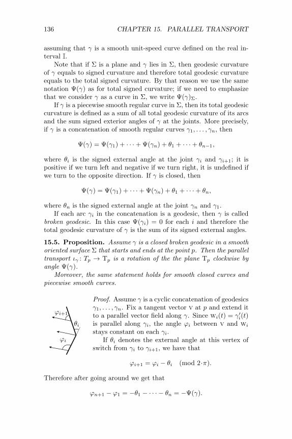
136 CHAPTER 15. PARALLEL TRANSPORT
assuming that γ is a smooth unit-speed curve defined on the real in-terval I.
Note that if Σ is a plane and γ lies in Σ, then geodesic curvatureof γ equals to signed curvature and therefore total geodesic curvatureequals to the total signed curvature. By that reason we use the samenotation Ψ(γ) as for total signed curvature; if we need to emphasizethat we consider γ as a curve in Σ, we write Ψ(γ)Σ.
If γ is a piecewise smooth regular curve in Σ, then its total geodesiccurvature is defined as a sum of all total geodesic curvature of its arcsand the sum signed exterior angles of γ at the joints. More precisely,if γ is a concatenation of smooth regular curves γ1, . . . , γn, then
Ψ(γ) = Ψ(γ1) + · · ·+ Ψ(γn) + θ1 + · · ·+ θn−1,
where θi is the signed external angle at the joint γi and γi+1; it ispositive if we turn left and negative if we turn right, it is undefined ifwe turn to the opposite direction. If γ is closed, then
Ψ(γ) = Ψ(γ1) + · · ·+ Ψ(γn) + θ1 + · · ·+ θn,
where θn is the signed external angle at the joint γn and γ1.If each arc γi in the concatenation is a geodesic, then γ is called
broken geodesic. In this case Ψ(γi) = 0 for each i and therefore thetotal geodesic curvature of γ is the sum of its signed external angles.
15.5. Proposition. Assume γ is a closed broken geodesic in a smoothoriented surface Σ that starts and ends at the point p. Then the paralleltransport ιγ : Tp → Tp is a rotation of the the plane Tp clockwise byangle Ψ(γ).
Moreover, the same statement holds for smooth closed curves andpiecewise smooth curves.
θi
ϕi
ϕi+1
Proof. Assume γ is a cyclic concatenation of geodesicsγ1, . . . , γn. Fix a tangent vector v at p and extend itto a parallel vector field along γ. Since wi(t) = γ′i(t)is parallel along γi, the angle ϕi between v and wi
stays constant on each γi.If θi denotes the external angle at this vertex of
switch from γi to γi+1, we have that
ϕi+1 = ϕi − θi (mod 2·π).
Therefore after going around we get that
ϕn+1 − ϕ1 = −θ1 − · · · − θn = −Ψ(γ).

137
Hence the the first statement follows.For the smooth unit-speed curve γ : [a, b]→ Σ, the proof is analo-
gous. If ϕ(t) denotes the angle between v(t) and w(t) = γ′(t), then
ϕ′(t) + kg(t) ≡ 0
Whence the angle of rotation
ϕ(b)− ϕ(a) =
b∫a
ϕ′(t)·dt =
= −b∫a
kg ·dt =
= −Ψ(γ)
The case of piecewise regular smooth curve is a straightforwardcombination of the above two cases.
Spherical area
If the contour ∂∆ of a spherical triangle with angles α, β and γ isoriented such that the triangle lies on the left, then its external anglesare π − α, π − β and π − γ. Therefore the total geodesic curvature of∂∆ is Ψ(∂∆) = 3·π − α− β − γ. The identity Ê can be rewritten as
Ê Ψ(∂∆) + area ∆ = 2·π.
The formula Ê holds for an arbitrary spherical polygon boundedby a simple broken geodesic. The latter can be proved by triangulatingthe poygon, applying the formula for each triangle in the triangulationand summing up the results.
βα
w
v
Q
R
If a spherical polygon is P divided intwo polygons Q and R by polygonal linebetween vertexes v and w then
Ψ(∂P ) + 2·π = Ψ(∂Q) + Ψ(∂R).
Indeed, for the internal angles Q and Rat v are α and β, then their externalangles are π − α and π − β respectfully.The internal angle of P in this case isα+β and its external angle is π−α−βClearly we have that
(π − α) + (π − β) = (π − α− β) + π;

138 CHAPTER 15. PARALLEL TRANSPORT
that is, the sum of external angles of Q and R at v is π plus theexternal angle of P at v. The same holds for the external angles atw and the rest of the external angles of P appear once on Q or R.Therefore if the formula Ê holds for Q and R, then it holds for P .
The following proposition gives a spherical analog of 6.5.
15.6. Proposition. Let P be a spherical polygon bounded by a simpleclosed broken geodesic ∂P . Assume ∂P is oriented such that P lies onthe left from ∂P . Then
Ψ(∂P ) + areaP = 2·π.
Moreover the same formula holds for any spherical region P boundedby piecewise smooth simple closed curve ∂P .
Sketch of proof. The proof of the first statement is given above.The second statement can be proved by approximation. One has to
show that the total geodesic curvature of an inscribed broken geodesicapproximates the total geodesic curvature of the original curve. Weomit the proof of the latter statement, but it can be done along thesame lines as 4.24.
15.7. Exercise. Assume γ is a simple piecewise smooth loop on S2
that divides its area into two equal parts. Denote by p the base pointof γ. Show that ιγ : TpS2 → TpS2 is the identity map.
Gauss–Bonnet formula
15.8. Theorem. Let ∆ be a topological disc in a smooth orientedsurface Σ bounded by a simple piecewise smooth and regular curve ∂∆that is oriented in such a way that ∆ lies on its left. Then
Ë Ψ(∂∆) +
∫∆
K = 2·π,
where K denotes the Gauss curvature of Σ.
For geodesic triangles this theorem was proved by Carl FriedrichGauss [16]; Pierre Bonnet and Jacques Binet independently general-ized the statement for arbitrary curves.
Note that if Σ is a plane, then the Gauss curvatue vanished; there-fore the statement of theorem follows from 6.5.
If Σ is the unit sphere, then K ≡ 1. Therefore formula Ë can berewritten as
Ψ(∂∆) + area ∆ = 2·π,

139
which follows from 15.6.We will give an informal proof of 15.8 in a partial case based on
the bike wheel interpretation described above. We suppose that it isintuitively clear that moving the axis of the wheel without changingits direction does not change the direction of the wheel’s spikes.
More precisely, assume we keep the axis of a non-spinning bikewheel and perform the following two experiments:
(i) We move it around and bring the axis back to the original po-sition. As a result the wheel might turn by some angle; let usmeasure this angle.
(ii) We move the direction of the axis the same way as before withoutmoving the center of the wheel. After that we measure the angleof rotation.
Then the resulting angles in these two experiments is the same.Consider a surface Σ with a Gauss map ν : Σ→ S2. Note that for
any point p on Σ, the tangent plane TpΣ is parallel to the tangentplane Tν(p)S2; so we can identify these tangent spaces. From theexperiments above, we get the following:
15.9. Lemma. Suppose α is a piecewise smooth regular curve in asmooth regular surface Σ which has a Gauss map ν : Σ → S2. Thenthe parallel transport along α in Σ coincides with the parallel transportalong the curve β = ν α in S2.
Proof of partial case of 15.8. We will prove the formula for proper sur-face Σ with positive Gauss curvature. In this case, by ?? the formulacan be rewritten as
Ì Ψ(∂∆) + area[ν(∆)] = 2·π.
The general case can be proved similarly, but one has to use the areaformula (A.5) and oriented area surrounded by a spherical curve.
Fix p ∈ ∂∆; assume the loop α runs along ∂∆ so that ∆ lies onthe left from it. Consider the parallel translation ι : Tp → Tp along α.According to 15.5, ι is a clockwise rotation by angle Ψ(α)Σ.
Set β = ν α. According to 15.9, ι is also parallel translation alongβ in S2. In particular ι is a clockwise rotation by angle Ψ(β)S2 . By15.6
Ψ(β)S2 + area[ν(∆)] = 2·π.Therefore ι is a counterclockwise rotation by area[ν(∆)]
Summarizing, the clockwise rotation by Ψ(α)Σ is identical to acounterclockwise rotation by area[ν(∆)]. The rotations are identicalif the angles are equal modulo 2·π. Therefore
Í Ψ(∂∆)Σ + area[ν(∆)] = 2·π ·n

140 CHAPTER 15. PARALLEL TRANSPORT
for an integer n.It remains to show that n = 1. By Í, this is so for a topological
disc in a plane. One can think of a general disc ∆ as about a resultof a continuous deformation of a plane disc. The integer n cannotchange in the process of deformation since the left hand side in Í iscontinuous along the deformation.
Let us redo the last argument more formally.First assume that ∆ lies in a local graph realization z = f(x, y)
of Σ. Consider one parameter family Σt of graphs z = t·f(x, y) anddenote by ∆t the corresponding disc in Σt, so ∆1 = ∆ amd ∆0 is itsprojection to the (x, y)-plane. Since Σ0 is a plane domain, we havearea[ν0(∆0)] = 0. Therefore by 6.5 we gave
Ψ(∂∆0)Σ0+ area[ν0(∆0)] = 2·π.
Note thatΨ(∂∆t)Σt + area[νt(∆t)]
depends continuously on t. According to Í, its value is a multipleof 2·π; therefore it has to be constant. Whence the Gauss–Bonnetformula follows.
If ∆ does not lie in one graph, then one could divide it into smallerdiscs, apply the formula for each and sum up the result. The proof isdone along the same lines as 15.6.
15.10. Exercise. Assume γ is a closed simple curve with constantgeodesic curvature 1 in a smooth closed surface Σ with positive Gausscurvature. Show that
length γ 6 2·π;
that is, the length of γ cannot exceed the length of the unit circle inthe plane.
15.11. Exercise. Let γ be a closed simple geodesic on a smooth closedsurface Σ with positive Gauss curvature. Assume ν : Σ → S2 is aGauss map. Show that the curve α = ν γ divides the sphere intoregions of equal area.
Conclude thatlengthα > 2·π.
a
b c
d
15.12. Exercise. Let Σ be a smooth closed surfacewith a closed geodesic γ. Assume γ has exactly 4self-intersection at the points a, b, c and d that ap-pear on γ in the order a, a, b, b, c, c, d, d. Show thatΣ cannot have positive Gauss curvature.

141
The following exercise gives the optimal bound on Lipschitz con-stant of a convex function that guarantees that its geodesics have noself-intersections; compare to 14.19.
15.13. Exercise. Suppose that f : R2 → R is a√
3-Lipschitz smoothconvex function. Show that any geodesic in the surface defined by thegraph z = f(x, y) has no self-intersections.
15.14. Advanced exercise. Let Σ be a smooth regular sphere withpositive Gauss curvature and p ∈ Σ. Suppose γ is a closed geodesic thatdoes not pass thru p. Assume Σ\p parametrized by the plane. Canit happen that in this parametrization, γ looks like one of the curveson the diagram? Say as much as possible about possible/impossible
diagrams of that type.
We start to study the intrinsic geometry of surfaces. The followingexercise should help you to be in the right mood for this; it might looklike a tedious problem in calculus, but actually it is an easy problemin geometry.
θ
15.15. Exercise. There is a mountain offrictionless ice with the shape of a perfect conewith a circular base. A cowboy is at the bot-tom and he wants to climb the mountain. So,he throws up his lasso which slips neatly overthe top of the cone, he pulls it tight and startsto climb. If the angle of inclination θ is large,there is no problem; the lasso grips tight andup he goes. On the other hand if θ is small, the lasso slips off as soonas the cowboy pulls on it.
What is the critical angle θ0 at which the cowboy can no longerclimb the ice-mountain?

142 CHAPTER 15. PARALLEL TRANSPORT
The remarkable theorem
Let Σ1 and Σ2 be two smooth regular surfaces in the Euclidean space.A map f : Σ1 → Σ2 is called length-preserving if for any curve γ1 inΣ1 the curve γ2 = f γ1 in Σ2 has the same length. If in addition fis smooth and bijective, then it is called intrinsic isometry.
A simple example of intrinsic isometry can obtained by warpinga plane into a cylinder. The following exercise produce slightly moreinteresting example.
15.16. Exercise. Suppose γ(t) = (x(t), y(t)) is a smooth unit-speedcurve in the plane such that y(t) = a· cos t. Let Σγ be the surface ofrevolution of γ around the x-axis. Show that a small open domain inΣγ admits a smooth length-pereserving map to the unit sphere.
Conclude that any round disc ∆ in S2 of intrinsic radius smallerthan π
2 admits a smooth length preserving deformation; that is, there isone parameter family of surfaces with boundary ∆t, such that ∆0 = ∆and ∆t is not congruent to ∆0 for any t 6= 0.1
15.17. Theorem. Suppose f : Σ1 → Σ2 is an intrinsic isometry be-tween two smooth regular surfaces in the Euclidean space; p1 ∈ Σ1 andp2 = f(p1) ∈ Σ1. Then
G(p1)Σ1 = G(p2)Σ2 ;
that is, the Gauss curvature of Σ1 at p1 is the same as the Gausscurvature of Σ2 at p2.
This theorem was proved by Carl Friedrich Gauss [16] who calledit Remarkable theorem (Theorema Egregium). The theorem is indeedremarkable because the Gauss curvature is defined as a product ofprinciple curvatures which might be different at these points; however,according to the theorem, their product can not change.
In fact Gauss curvature of the surface at the given point can befound intrinsically, by measuring the lengths of curves in the surface.For example, Gauss curvature G(p) in the following formula for thecircumference c(r) of a geodesic circle centered at p in a surface:
c(r) = 2·π ·r − π3 ·G(p)·r3 + o(r3).
Note that the theorem implies there is no smooth length-preservingmap that sends an open region in the unit sphere to the plane.2 It
1In fact any disc in S2 of intrinsic radius smaller than π admits a smooth lengthpreserving deformation.
2There are plenty of non-smooth length-preserving maps from the sphere to theplane; see [31] and the references there in.

143
follows since the Gauss curvature of the plane is zero and the unitsphere has Gauss curvature 1. In other words, there is no map of aregion on Earth without distortion.
Proof. Set g1 = G(p1)Σ1and g2 = G(p2)Σ2
; we need to show that
Î g1 = g2.
Suppose ∆1 is a small geodesic triangle in Σ1 that contains p1.Set ∆2 = f(∆1). We may assume that the Gauss curvature is almostconstant in ∆1 and ∆2; that is, given ε > 0, we can assume that
Ï|G(x1)Σ1 − g1| < ε,
|G(x2)Σ2 − g2| < ε
for any x1 ∈ ∆1 and x2 ∈ ∆2.Since f is length-preserving the triangles ∆2 is geodesic and
Ð area ∆1 = area ∆2.
Moreover, triangles ∆1 and ∆2 have the same corresponding angles;denote them by α, β and γ.
By Gauss–Bonnet formula, we get that
Ñ
∫∫∆1
GΣ1= α+ β + γ − π =
∫∫∆2
GΣ2.
By Ï, ∣∣∣∣∣∣g1 −1
area ∆1·∫∫∆1
GΣ1
∣∣∣∣∣∣ < ε,
∣∣∣∣∣∣g2 −1
area ∆2·∫∫∆2
GΣ2
∣∣∣∣∣∣ < ε.
By Ð and Ñ,
1
area ∆1·∫∫∆1
GΣ1=
1
area ∆2·∫∫∆2
GΣ2,
therefore|g1 − g2| < 2·ε.
Since ε > 0 is arbitrary, Î follows.
144 CHAPTER 15. PARALLEL TRANSPORT
Simple geodesic
The following theorem provides an interesting application of Gauss–Bonnet formula; it is proved by Stephan Cohn-Vossen [Satz 9 in 9].
15.18. Theorem. Any open smooth regular surface with positiveGauss curvature has a simple two-sided infinite geodesic.
15.19. Lemma. Suppose Σ is an open surface in with positive Gausscurvature in the Euclidean space. Then there is a convex function fdefined on a convex open region of (x, y)-plane such that Σ can bepresented as a graph z = f(x, y) in some (x, y, z)-coordinate system ofthe Euclidean space.
Moreover
Ò
∫∫Σ
G 6 2·π.
Proof. The surface Σ is a boundary of an unbounded closed convexset K.
Fix p ∈ Σ and consider a sequence of points xn such that |xn−p| →→ ∞ as n → ∞. Set un = xn−p
|xn−p| ; the unit vector in the direction
from p to xn. Since the unit sphere is compact, we can pass to asubsequence of (xn) such that un converges to a unit vector u.
Note that for any q ∈ Σ, the directions vn = xn−q|xn−q| converge to u
as well. The half-line from q in the direction of u lies in K. Indeed anypoint on the half-line is a limit of points on the line segments [q, xn];since K is closed, all of these poins lie in K.
Let us choose the z-axis in the direction of u. Note that line seg-ments can not lie in Σ, otherwise its Gauss curvature would vanish.It follows that any vertical line can intersect Σ at most at one point.That is, Σ is a graph of a function z = f(x, y). Since K is convex, thefunction f is convex and it is defined in a region Ω which is convex.The domain Ω is the projection of Σ to the (x, y)-plane. This pro-jection is injective and by the inverse function theorem, it maps opensets in Σ to open sets in the plane; hence Ω is open.
It follows that the outer normal vectors to Σ at any point, pointsto the south hemisphere S2
− =
(x, y, z) ∈ S2 : z < 0
. Therefore thearea of the spherical image of Σ is at most area S2
− = 2·π. The area

145
of this image is the integral of the Gauss curvature along Σ. That is,∫∫Σ
G = area[ν(Σ)] 6
6 area S2− =
= 2·π,
where ν(p) denotes the outer unit normal vector at p. Hence Ò follows.
Proof of 15.18. Let Σ be an open surface in with positive Gausscurvature and γ a two-sided infinite geodesic in Σ. The following isthe key statement in the proof.
15.20. Claim. The geodesic γ contains at most one simple loop.
Assume γ has a simple loop `. By Lemma 15.19, Σ is parameterizedby a open convex region Ω in the plane; therefore ` bounds a disc inΣ; denote it by ∆. If ϕ is the angle at the base of the loop, then byGauss–Bonnet, ∫∫
∆
G = π + ϕ.
By Lemma 15.19, ϕ < π; that is, γ has no concave simple loopsAssume γ has two simple loops, say `1 and `2 that bound discs ∆1
and ∆2. Then the disks ∆1 and ∆2 have to overlap, otherwise thecurvature of Σ would exceed 2·π.
We may assume that ∆1 6⊂ ∆2; the loop `2 appears after `1 onγ and there are no other simple loops between them. In this case,after going around `1 and before closing `2, the curve γ must enter ∆1
creating a concave loop. The latter contradicts the above observation.If a geodesic γ has a self-intersection, then it contains a simple
loop. From above, there is only one such loop; it cuts a disk from Σand goes around it either clockwise or counterclockwise. This way wedivide all the self-intersecting geodesics into two sets which we will callclockwise and counterclockwise.
Note that the geodesic t 7→ γ(t) is clockwise if and only if thesame geodesic traveled backwards t 7→ γ(−t) is counterclockwise. Byshooting unit-speed geodesics in all directions at a given point p =γ(0), we get a one parameter family of geodesics γs for s ∈ [0, π]connecting the geodesic t 7→ γ(t) with the t 7→ γ(−t); that is, γ0(t) == γ(t) and γπ(t) = γ(−t). It follows that there are geodesics whicharen’t clockwise nor counterclockwise. Those geodesics have no self-intersections.

Part IV
Background material
146

Appendix A
Multivariable calculus
Regular values
A map f : Rn → Rk can be thought as an array of functions
f1, . . . , fk : Rn → R.
The map f is called smooth if each function fi is smooth; that is, allpartial derivatives of fi are defined in the domain of definition of f .
The following matrix
Jacx f =
∂f1
∂x1· · · ∂f1
∂xn...
. . ....
∂fk∂x1
· · · ∂fk∂xn
is called Jacobian matrix of f ; we assume that the right hand side isevaluated at x = (x1, . . . , xn).
Inverse function theorem gives a sufficient condition for a smoothfunction to be invertible in a neighborhood of a given point p in itsdomain. The condition is formulated in terms of the partial derivativesof fi at p.
Implicit function theorem is a close relative to inverse functiontheorem; in fact it can be obtained as its corollary. It is used forinstance when we need to pass from parametric to implicit descriptionof curves and surfaces.
Both theorems reduce the existence of a map satisfying certainequation to a question in linear algebra that can be written in termsof its Jacobian matrix. We use these two theorems only for n 6 3.
147

148 APPENDIX A. MULTIVARIABLE CALCULUS
These two theorems are discussed in any course of multivariablecalculus, the classical book of Walter Rudin [32] is one of my favorites.
A.1. Inverse function theorem. Let f = (f1, . . . , fn) : Rn → Rnbe a smooth map. Assume that the Jacobian matrix
∂f1
∂x1· · · ∂f1
∂xn...
. . ....
∂fn∂x1
· · · ∂fn∂xn
is invertible at some point p in the domain of definition of f . Thenthere is a smooth function h : Rm → Rn defined in a neighborhoodΩq of q = f(p) that is a local inverse of f at p; that is, there is aneighborhood Ωp 3 p such that f defines a bijection Ωp → Ωq and(h) f(x) = x for any x ∈ Ωp.
A.2. Implicit function theorem. Let f = (f1, . . . , fn) : Rn+m →Rn be a smooth map, m,n > 1. Let us consider Rn+m as a productspace Rn × Rm with coodinates x1, . . . , xn, y1, . . . , ym. Consider thefollowing matrix
M =
∂f1
∂x1· · · ∂f1
∂xn...
. . ....
∂fn∂x1
· · · ∂fn∂xn
formed by the first n columns of the Jacobian matrix. Assume Mis invertible at some point p in the domain of definition of f andf(p) = 0. Then there is a neighborhood Ωp 3 p and a smooth functionh : Rm → Rn defined in a neighborhood Ω0 3 0 such that for any(x1, . . . , xn, y1, . . . ym) ∈ Ωp, the equality
f(x1, . . . , xn, y1, . . . ym) = 0
holds if and only if
(x1, . . . xn) = h(y1, . . . ym).
If the assumption in the theorem holds for any point p such thatf(p) = 0, then we say that 0 is a regular value of f . The followinglemma states that most values of a smooth map are regular; in partic-ular, generic smooth functions satisfy the assumption of the theorem.
149
A.3. Sard’s lemma. Given a smooth map f : U → Rm defined onan open set U ⊂ Rn, most of the values in Rm are regular.
The words almost all means all values, with the possible exceptionof a set of zero Lebesgue measure. In particular if one chooses arandom value equidistributed in an arbitrarily small ball B ⊂ Rm,then it is a regular value of f with probability 1.
Multiple integral
Setjacx f := |det[Jacx f ]|;
that is, jacx f is the absolute value of the determinant of the Jacobianmatrix of f at x.
The following theorem is a substitution rule for multiple variables.
A.4. Theorem. Let K ⊂ Rn be a compact set and h : K → R bea bounded measurable function. Assume f : K → Rn is an injectivesmooth map. Then∫
K
h(x)· jacx f ·dx =
∫f(K)
h f−1(y)·dy.
A.5. Area formula. Let f : K → Rn be a smooth map defined on acompact set K ⊂ Rn. Then for any function h : K → R∫
K
h(x)· jacx f ·dx =
∫f(K)
HK(y)·dy,
whereHK(y) =
∑x∈K
f(x)=y
h(x).
(The integrals are understood in the sense of Lebesgue.)
Let us sketch the proof of area formula using Sard’s lemma (A.3)and the substitution rule (A.4).
Sketch of proof. Denote by S ⊂ K the set of critical points of f ; thatis, x ∈ S if jacx f = 0. By Sard’s lemma, f(S) has vanishing measure.Note that ∫
S
h(x)· jacx f ·dx = 0

150 APPENDIX A. MULTIVARIABLE CALCULUS
since jacx f = 0 and ∫f(S)
HS(y)·dy
since f(S) has vanishing measure. In particular,∫S
h(x)· jacx f ·dx =
∫f(S)
HS(y)·dy;
that is the area formula holds for S.It remains to prove that∫
K\S
h(x)· jacx f ·dx =
∫f(K\S)
HK\S(y)·dy.
Since jacx f 6= 0 for any x ∈ K\S, by inverse function theorem,the restriction of f to a neighborhood U 3 x has a smooth inverse.Therefore for any compact set K ′ ⊂ U we have that∫
K′
h(x)· jacx f ·dx =
∫f(K1)
h(f−1(y))·dy.
It remains to subdivide K1 into a countable collection of subsets ofthat type and sum up the corresponding formulas.
Divergence theorem
A.6. Theorem. If a piecewise smooth surface Σ bounds a body V inR3, then
fluxu Σ =
∫∫∫V
divu,
assuming that the orientation on Σ is defined by a unit normal fieldthat points out of V .
Curl theorem
Given a vector field u, set curlu := ∇×u; that is, if we write the fieldu in the standard basis
u = P ·i +Q·j +R·j,
151
then
curlu :=(∂R∂y −
∂Q∂z
)·i +
(∂P∂z −
∂R∂x
)·j +
(∂Q∂x −
∂P∂y
)·k
A.7. Theorem. Let Σ be a compact oriented surface bounded by acurve γ. Assume that γ : [0, `]→ R3 is parameterized by its arc-lengthand oriented in such a way that Σ lies on left from it. Then, for anysmooth vector field defined in a neighborhood of Σ, we have
fluxcurl u Σ =
`∫0
〈u, γ′(t)〉·dt.

Appendix B
Differential equations
Initial value problem
The following theorem guarantees existence and uniqueness of solu-tions of an initial value problem for a system of ordinary differentialequations
x′1(t) = f1(x1, . . . , xn, t),
. . .
x′n(t) = fn(x1, . . . , xn, t),
where each xi = xi(t) is a real valued function defined on a real intervalI and each fi is a smooth function defined on Rn × I.
The array of functions (f1, . . . , fn) can be considered as one vector-valued function f : Rn × I → Rn and the array (x1, . . . , xn) can beconsidered as a vector x ∈ Rn. Therefore the system can be rewrittenas one vector equation
x′(t) = f(x, t).
B.1. Theorem. Suppose I is a real interval and f : Rn×I→ Rn is asmooth function. Then for any initial data x(t0) = u the differentialequation
x′(t) = f(x, t)
has a unique solution x(t) defined at a maximal subinterval J of I thatcontains t0. Moreover
(a) if J 6= I (that is, if an end a of J lies in the interior of I) thenx(t) diverges as t→ a;
(b) the function (u, t0, t) 7→ x(t) is smooth.
152

Appendix C
Real analysis
Lipschitz condition
Recall that a function f between metric spaces is called Lipschitz ifthere is a constant L such that
|f(x)− f(y)| 6 L·|x− y|
for all values x and y in the domain of definition of f .
C.1. Rademacher’s theorem. Let f : [a, b] → R be a Lipschitzfunction. Then the derivative f ′(x) is defined for alomst all x ∈ [a, b].Moreover the derivative f ′ is a bounded measurable function definedalmost everywhere in [a, b] and it satisfies the fundamental theorem ofcalculus; that is, the following identity
f(b)− f(a) =
b∫a
f ′(x)·dx,
holds if the integral is understood in the sense of Lebesgue.
The following theorem makes possible to extend many statementsabout continuous function to measurable functions.
C.2. Lusin’s theorem. Let ϕ : [a, b]→ R be a measurable function.Then for any ε > 0, there is a continuous function ψε : [a, b] → Rthat coincides with ϕ outside of a set of measure at most ε. Moreover,if ϕ is bounded above and/or below by some constants, then we mayassume that so is ψε.
153

154 APPENDIX C. REAL ANALYSIS
Uniform continuity and convergence
Let f be a real function defined on a real interval. If for any ε > 0there is δ > 0 such that
|x1 − x2|X < δ =⇒ |f(x1)− f(x2)|Y < ε,
then f is called uniformly continuous.Evidently every uniformly continuous function is continuous; the
converse does not hold. For example, the function f(x) = x2 is con-tinuous, but not uniformly continuous.
However if f is continuous and defined on a closed interval [a, b],then f is uniformly continuous
If the condition above holds for any function fn in a sequenceand δ depend solely on ε, then the sequence (fn) is called uniformlyequicontinuous. More precisely, a sequence of functions fn : X → Yis called uniformly equicontinuous if for any ε > 0 there is δ > 0 suchthat
|x1 − x2|X < δ =⇒ |fn(x1)− fn(x2)|Y < ε
for any n. Uniform equicontinuity is the condition in one of the mostimportant convergence theorems in analysis. We say that a sequence offunctions fi : X → Y converges uniformly to a function f∞ : X → Yif for any ε > 0, there is a natural number N such that for all n ≥ N ,we have |f∞(x)− fn(x)| < ε for all x ∈ X.
C.3. Arzela-Ascoli Theorem. Any uniformly equicontinuous se-quence of function fn : [a, b]→ [c, d] has a subsequence that convergesuniformly to a continuous function.

Appendix D
Topology
Jordan’s theorem
We sometimes use the following characterization of homeomorphismsbetween compact spaces.
D.1. Theorem. A continuous bijection f between compact metricspaces has a continuous inverse; that is, f is a homeomorphism.
The first part of the following theorem was proved by Camille Jor-dan, the second part is due to Arthur Schoenflies.
D.2. Theorem. The complement of any closed simple plane curve γhas exactly two connected components.
Moreover, there is a homeomorphism h : R2 → R2 that maps theunit circle to γ. In particular γ bounds a topological disc.
This theorem is known for its simple formulation and quite hardproof. By now many proofs of this theorem are known. For the firststatement, a very short proof based on a somewhat developed tech-nique is given by Patrick Doyle [11], among elementary proofs, one ofmy favorites is the proof given by Aleksei Filippov [13].
We use the following smooth analog of this theorem.
D.3. Theorem. The complement of any closed simple smooth reg-ular plane curve γ has exactly two connected components.
Moreover the there is a diffeomorphism h : R2 → R2 that maps theunit circle to γ.
The proof of this statement is much simpler. An amusing proofcan be found in [8].
155

156 APPENDIX D. TOPOLOGY
Connectedness
Recall that a continuous map α from the unit interval [0, 1] to a metricspace is called a path. If p = α(0) and q = α(1), then we say that αconnects p to q.
A set X in the Euclidean space is called path connected if any twopoints x, y ∈ X can be connected by a path lying in X.
A set X in the Euclidean space is called connected if one cannotcover X with two disjoint open sets V and W such that both intersec-tions X ∩ V and X ∩W are nonempty.
D.4. Proposition. Any path connected set is connected. Moreover,any open connected set in the Euclidean space or plane is path con-nected.
Given a point x ∈ X, the maximal connected subset of X contain-ing x is called the connected component of x in X.

Appendix E
Elementary geometry
E.1. Theorem. The sum of all the internal angles of a simple n-gonis (n− 2)·π.
Proof. The proof is by induction on n. For n = 3 it says that sum ofinternal angles of a triangle is π, which is assumed to be known.
First let us show that for any n > 4, any n-gon has a diagonal thatlies inside of it. Assume this holds true for all polygons with at mostn− 1 vertices.
Fix an n-gon P , n > 4. Applying a rotation if necessary, we canassume that all its vertexes have different x-coordinates. Let v bea vertex of P that minimizes the x-coordinate; denote by u and wits adjacent vertexes. Let us choose the diagonal uw if it lies in P .Otherwise the triangle 4uvw contains another vertex of P . Choosea vertex s in the interior of 4uvw that maximizes the distance toline uw. Note that the diagonal vs lies in P ; if it is not the case,then vs crosses another side pq of P , one of the vertices p or q haslarger distance to the line and it lies in the interior of 4uvw — acontradiction.
Note that the diagonal divides P into two polygons, say Q and R,with smaller number of sides in each, say k and m correspondingly.Note that
Ê k +m = n+ 2;
indeed each side of P appears once as a side of P or Q plus the diagonalappears twice — once as a side in Q and once as a side of R. Notethat the sum of the angles of P is the sum of the angles of Q andR, which by the induction hypothesis are (k − 2)·π and (m − 2)·π
157

158 APPENDIX E. ELEMENTARY GEOMETRY
correspondingly. It remains to note that Ê implies
(k − 2)·π + (m− 2)·π = (n− 2)·π.
Triangle inequality for angles
The following theorem says that the triangle inequality holds for anglesbetween half-lines from a fixed point. In particular it implies that asphere with the angle metric is a metric space.
E.2. Theorem. The inequality
]aob+ ]boc > ]aoc
holds for any three half-lines oa, ob and oc in the Euclidean space.
The following lemma says that the angle of a triangle monotonicallydepends on the opposit side, assuming the we keep the other two sidesfixed. It follows directly from the cosine rule.
E.3. Lemma. Let x, y, z, x′, y′ and z′ be 6 points such that |x−y| =|x′ − y′| > 0 and |y − z| = |y′ − z′| > 0. Then
]xyz > ]x′y′z′ if and only if |x− z| > |x′ − z′|.
o a
b′
b
cProof of E.2. We can assume that ]aob < ]aoc;otherwise the statement is evident. In this casethere is a half-line ob′ in the angle aoc such that
]aob = ]aob′,
so in particular we have that
]aob′ + ]b′oc = ]aoc.
Without loss of generality we can assume that |o− b| = |o− b′| and b′
lies on a line segment ac, so
|a− b′|+ |b′ − c| = |a− c|.
Then by the triangle inequality
Ë|a− b|+ |b− c| > |a− c| =
= |a− b′|+ |b′ − c|.
159
Note that in the triangles aob and aob′ the side ao is shared, so]aob = ]aob′ and |o − b| = |o − b′|. By side-angle-side congruencecondition, we have that 4aob ∼= 4aob′; in particular |a− b′| = |a− b|.Therefore from Ë we get
|b− c| > |b′ − c|.
Applying the angle monotonicity (E.3) we obtain
]boc > ]b′oc.
Whence
]aob+ ]boc > ]aob′ + ]b′oc =
= ]aoc.
Convexity
A set X in the Euclidean space is called convex if for any two pointsx, y ∈ X, any point z between x and y lies in X. It is called strictlyconvex if for any two points x, y ∈ X, any point z between x and ylies in the interior of X.
From the definition, it is easy to see that the intersection of anarbitrary family of convex sets is convex. The intersection of all convexsets containing X is called the convex hull of X; it is the minimalconvex set containing the set X.
We will use the following corollary of the so called hyperplane sep-aration theorem:
E.4. Lemma. Let K ⊂ R3 be a closed convex set. Then for anypoint p /∈ K there is a plane Π that separates K from p; that is, Kand p lie on opposite open half-spaces separated by Π.
A function of two variables (x, y) 7→ f(x, y) is called convex if itsepigraph z > f(x, y) is a convex set. This is equivalent to the so-calledJensen’s inequality
f (t·x1 + (1− t)·x2) ≤ t·f(x1) + (1− t)·f(x2)
for t ∈ [0, 1]. If f is smooth, then the condition is equivalent to thefollowing inequality for the second directional derivative:
D2wf > 0
for any vector w 6= 0 in the (x, y)-plane.

Appendix F
Area
Area of spherical triangle
F.1. Lemma. Let ∆ be a spherical triangle; that is, ∆ is the inter-section of three closed half-spheres in the unit sphere S2. Then
Ê area ∆ = α+ β + γ − π,
where α, β and γ are the angles of ∆.
The value α+ β + γ − π is called excess of the triangle ∆.
∆∆∆∆∆∆∆∆∆∆∆∆∆∆∆∆∆∆∆∆∆∆∆∆∆∆∆∆∆∆∆∆∆∆∆∆∆∆∆∆∆∆∆∆∆∆∆∆∆∆∆∆∆∆∆∆∆∆∆∆∆∆∆∆∆
Proof. Recall that
Ë area S2 = 4·π.
Note that the area of a spherical slice Sα betweentwo meridians meeting at angle α is proportional to α.Since for Sπ is a half-sphere, from Ë, we get areaSπ =
= 2·π. Therefore the coefficient is 2; that is,
Ì areaSα = 2·α.
Extending the sides of ∆ we get 6 slices: two Sα, two Sβ and twoSγ which cover most of the sphere once, but the triangle ∆ and itscentrally symmetric copy ∆′ are covered 3 times. It follows that
2· areaSα + 2· areaSβ + 2· areaSγ = areaS2 + 4· area ∆.
Substituting Ë and Ì and simplifying, we get Ê.
160

161
Schwarz’s boot
Recall that we defined length of curve as the exact upper bound onthe length of inscribed polygonal lines. It suggests to define area of asurface as a exact upper bound on the area of polyhedrons inscribedin the surface.
However as you will see from the following example, this idea failsbadly even for cylindrical surface. Namely, we will show that if we de-fine the area as the least upper bound of areas of inscribed polyhedralsurfaces, then the area of the lateral surface of the cylinder must beinfinite. The latter contradicts correct intuition that the area of thissurface should be the product of the circumference of the base circleand the height of the cylinder.
Let us divide the cylinder into mequal cylinders by planes parallel to itsbase. This way we obtain m + 1 cir-cles on the lateral surface of a cylinder,including both bases. Further, let us di-vide each of these circles into n equalarcs in such a way that the dividingpoints of a circle will lie exactly abovethe midpoints of arcs on the circle un-der it. Consider all triangles formed bya chord of such arc and line segments connecting the ends of the chordwith the points right above and right below the mid point of its arc.All the 2mn equal triangles form a polyhedral surface which is calledSchwarz’s boot. A Schwarz’s boot for m = 8 and n = 6 is shown onthe diagram.
a
bbbbbbbbbbbbbbbbbbbbbbbbbbbbbbbbbbbbbbbbbbbbbbbbbbbbbbbbbbbbbbbbb
b′c
p
Consider one of the triangle abc whichform the Schwarz’s boot. By construc-tion, its base ac lies in a horizontal planeand the projection b′ of b on this plane bi-sects the arc ac. Therefore the vertexes ofthe triangle ab′c are the three consequentvertexes of a regular 2n-gone inscribed ina unit circle. Denote the triangle ab′c bysn; clearly it depends only on n and the radius of the base.
Both triangles abc and ab′c are isosceles with shares base ac. Note

162 APPENDIX F. AREA
that the altitude bp is larger than the altitude b′p. Therefore
area(4abc) = 12 ·|a− c|·|b− p| >
> 12 ·|a− c|·|b
′ − p| == area(4ab′c) =
= sn.
In particular,Sm,n > 2·m·n·sn,
where Sm,n denotes the total area of the Schwarz’s boot. Consider thepairs (m,n) such that m is much larger than n; namely m > 1
sn. Then
Sm,n > 2·m·n·sn > 2· 1sn·n·sn = 2·n.
Therefore Sm,n →∞ as n→∞.

Part V
Semisolutions
163

164
1.1. Check all the conditions in the definition of metric, page 6.
1.2; (a). Observe that |p− q|X 6 1. Apply the triangle inequality toshow that |p− x|X 6 2 for any x ∈ B[q, 1]. Make a conclusion.
(b). Take X to be a half-line [0,∞) with the standard metric; p = 0and q = 4
5 .
1.5. Show that the conditions in 1.4 hold for δ = ε.
1.8. Suppose the complement Ω = X\Q is open. Then for each pointp ∈ Ω there is ε > 0 such that |p − q|X > ε for any q ∈ Q. It followsthat p is not a limit point of any sequence qn ∈ Q. That is, any limitof points in Q lies in Q which by definition means that Q is closed.
Now suppose Ω = X\Q is not open. Then there is a point p ∈ Ωsuch that for any natural n there is a point qn ∈ Q such that |p−qn|X << 1
n ; in particular qn → p and n→∞. Since p /∈ Q, we get that Q isnot closed.
2.2. The image of γ might have a shape of digit 8 or 9.
2.3. Let α be a path connecting p to q.Passing to a subinterval if necessary, we can assume that α(t) 6= p, q
for t 6= 0, 1.An open set Ω in (0, 1) will be called suitable if for any connected
component (a, b) of Ω we have α(a) = α(b). Show that the unionof nested suitable sets is suitable. Therefore we can find a maximalsuitable set Ω.
Define β(t) = α(a) for any t in a connected component (a, b) ⊂ Ω.Note that for any x ∈ [0, 1] the set β−1β(x) is connected.
It remains to re-parametrize β to make it injective. In other wordswe need to construct a non-decreasing surjective function τ : [0, 1] →→ [0, 1] such that τ(t1) = τ(t2) if and only if there is a connectedcomponent (a, b) such that t1, t2 ∈ [a, b]. The construction is similarto the construction of devil’s staircase.
2.4. Denote the union of two half-axis by L. Observe that f(t)→∞as t → ∞. Since f(0) = 0, the intermediate value theorem impliesthat f(t) takes all nonnegative values for t > 0. Use it to show that Lis the range of α.
Note that the function f is smooth. Indeed, the existence of allderivatives f (n)(x) at x 6= 0 is evident and direct calculations showthat f (n)(0) = 0 for all n. Therefore t 7→ α(t) = (f(t), f(−t)) issmooth as well.
Further, show that the function f is strictly increasing for t > 0,and, moreover, if 0 < t0 < t1, then 0 < f(t0) < f(t1). Use it to showthat the maps t 7→ α(t) is injective.

165
Summarizing we get that α is a smooth parametrization of L.Now suppose β : t 7→ (x(t), y(t)) is a smooth parameterization of L.
Without loss of generality we may assume that x(0) = y(0) = 0. Notethat x(t) > 0 for any t therefore x′(0) = 0. The same way we get thaty′(0) = 0. That is, β′(0) = 0; so L does not admit a smooth regularparameterization.
2.5. Apply the definitions. For (a) you need to check that γ′` 6= 0.For (b) you need to check that γ`(t0) = γ(t1) only if t0 = t1.
2.6. This is so called semicubical parabola; it is shownon the diagram. Try to argue similarly to 2.4.
2.7. For ` = 0 the system describes a pair of points(0, 0,±1), so we can assume that ` 6= 0. Note thatfirst equation desribes the unit sphere centered at theorigin and the second equation describes a cylinderover the circle in the (x, y)-plane with diameter withopposite points (0, 0) and (0, `).
For ` 6= 0, find the gradients ∇f and ∇h for thefunctions
f(x, y, z) = x2 + y2 + z2 − 1
h(x, y, z) = x2 + `·x+ y2
and show that they are linearly dependent only onthe x-axis. Conclude that for ` 6= ±1 each connectedcomponent of the set of solutions is a smooth regularcurve.
Show that if |`| < 1, then the set has two connected components with z > 0
and z < 0. if |`| > 1, then the set is connected.
xy
zNote that the condition on gradients pro-
vides only sufficient condition. Therefore hecase ` = ±1 has to be checked by hands. Inthis case a neighborhood of (±1, 0, 0) doesnot admit a smooth regular parametrization— try to prove it. The case ` = 0 shown onthe diagram.
Remark. In the case ` = ±1 it is calledViviani’s curve. It admits the followingsmooth regular parameterization with a self-intersection:
t 7→ (±(cos t)2, cos t· sin t, sin t).

166
2.8. Without loss of generality we may assume that the origin doesnot lie on the curve.
Show that inversion of the plane (x, y) 7→ ( xx2+y2 ,
yx2+y2 ) maps our
curve maps to a closed curve with removed origin. Apply Jordan’stheorem for the obtained curve and use the inversion again.
3.2. Observe that if c = τ0 < · · · < τn = d is a partition of [c, d] ifand only if ti = ϕ(τi) is a partition of [a, b] and apply the definition oflength (3.1).
3.3. Fix a partition 0 = t0 < · · · < tn = 1 of [0, 1]. Set τ0 = 0 andτi = max τ ∈ [0, 1] : β(τi) = α(ti) . Show that (τi) is a partition of[0, 1]; that is, 0 = τ0 < τ1 < · · · < τn = 1.
By construction
|α(t0)− α(t1)|+ |α(t1)− α(t2)|+ · · ·+ |α(tn−1)− α(tn)| == |β(τ0)− β(τ1)|+ |β(τ1)− β(τ2)|+ · · ·+ |β(τn−1)− β(τn)|.
Since the partition (ti) is arbitrary, we get
lengthβ > lengthα.
Remark. Note that the partition (τi) is not arbitrary, therefore theinequality might be strict; it might happen if β runs back and forthalong α.
3.4. For (3.4a), apply the fundamental theorem of calculus for eachsegment in a given partition. For (3.4b) consider a partition such thatthe velocity vector α′(t) is nearly constant on each of its segments.
3.5. Use theorems of Rademacher and Lusin (C.1 and C.2).
3.6.
3.8. We have to assume that a 6= 0 or b 6= 0; otherwise we get aconstant curve.
Show that the curve has constant velocity |γ′(t)| ≡√a2 + b2.
Therefores = t√
a2+b2
is an arc-length parameter.
3.12. Choose a closed polygonal line p1 . . . pn inscribed in β. By 3.11,we can assume that it length is arbitrary close to the length of β; thatis, given ε > 0
length(p1 . . . pn) > lengthβ − ε.
Show that we may assume in addition that each point pi lies on α.

167
Observe that since α is simple, the points p1, . . . , pn appear on αin the same cyclic order; that is, the polygonal line p1 . . . pn is alsoinscribed in α. In particular
lengthα > length(p1 . . . pn).
It follows thatlengthα > lengthβ − ε.
for any ε > 0. Whence
lengthα > lengthβ.
p1 p2
pn
...
If α has self-intersections, then the pointsp1, . . . , pn might appear on α in a different order,say pi1 , . . . , pin . Apply triangle inequality to showthat
length(pi1 . . . pin) > length(p1 . . . pn)
and use it to modify the proof above.
3.13. Denote by `u the line segment obtained orthogonal projectionof γ to the line in the direction u. Note that γu runs back and forthalong `u, we get
length γu > 2· length `u.
Applying the Crofton formula, we get that
length γ > π ·length `u.
In the case of equality, the curve γu runs exactly back and forthalong `u without additional zigzags for almost all (and therefore forall) u.
Let K be a closed set bounded by γ. Observe that the last state-ment implies that every line may intersect K only along a closed seg-ment. In other words K is convex.
3.14. The proof is identical to the proof of the standard Croftonformula. To find the coefficient one has to find average length ofprojection of unit vector to a line. Which can be done by integration.
1
ka=
1
area S2·∫S2
|x|; 1
kb=
1
area S2·∫S2
√1− x2.
The answers are ka = 2 and kb = 4π .
3.16.

168
3.17. The “only-if” part is trivial. To show the “if” part, assume Ais not convex; that is, there are points x, y ∈ A and a point z /∈ A thatlies between x and y.
Since A is closed, its complement is open. That is, the ball B(z, ε)does not intersect A for some ε > 0.
Show that there is δ > 0 such that any path of length at most|z− y|R3 + δ pass thru B(z, ε). It follows that |z− y|A > |z− y|R3 + δ,in particular|z − y|A 6= |z − y|R3 .
x
y z
−x
−y−z
3.20. The spherical curve shown on the diagramdoes not have antipodal pairs of points. Howeverit has three points x, y, z on one of its sides andtheir antipodal points −x,−y,−z on the other.Show that this property is sufficient to concludethat the curve does not lie in any hemisphere.
3.21. Assume contrary, then by the hemispherelemma (3.19) γ lies in an open hemisphere. Inparticular it cannot divide S2 into two regionsof equal area — a contradiction.
3.22. The very first sentence is wrong — it is not sufficient to showthat diameter iis at most 2. For example an equilateral triangle withcircumradius slightly above 1 may have diameter (which is defined asthe maximal distance between its points) slightly bigger than
√3, so
it can be made smaller that 2.On the other hand, it is easy to modify the proof of the hemisphere
lemma (3.19) to get a correct solution. That is, (1) choose two pointsp and q on γ that divide it into two arcs of the same length; (2) set zto be a midpoint of p and q, and (3) show that γ lies in the unit disccentered at z.
3.23. For (a), modify the proof of the original Crofton formula [seepage 20].
(b). Assume length γ < 2·π. By (a),
length γu < 2·π.
Therefore we can choose u so that
length γu < 2·π.
Observe that γu runs in a semicircle h and therefore γ lies in ahemisphere with h as a diameter.
4.2. Differentiate the identity 〈γ(s), γ(s)〉 = 1 a couple of times.

169
4.3. Prove and use the following identities:
γ′′(t)− γ′′(t)⊥ = γ′(t)|γ′(t)| ·〈γ
′′(t), γ′(t)|γ′(t)| 〉,
|γ′(t)| =√〈γ′(t), γ′(t)〉.
4.4. Apply 4.3a for the parameterization t 7→ (t, f(t)).
4.5. Show that γ′′a,b ⊥ γ′a,b and apply 4.3a.
4.8. Apply Fenchel’s theorem.
4.9. Assume that γ is unit-speed; show that |σ′| 6 κ + θ′, whereθ(s) = ](γ(s), γ′(s)).
4.12. Set α = ](w,u) and β = ](w,v). Try to guess the examplefrom the diagram.
pq
v w
u
u
I
II III
The shown curve is divided into three arcs: I, II, and III. Arc Iturns from v to u; it has total curvature α. Analogously the arc IIIturns from u to w and has total curvature β. Arc II goes very closeand almost parallel to the chord pq and its total curvature can bemade arbitrary small.
4.13. Use that exterior angle of a triangle equals to the sum of thetwo remote interior angles; for the second part apply the induction onnumber of vertexes.
4.15. An example for (a) is shown on the diagram.
(b). Assume x is a point of self-intersection. Showthat we may choose two points y and z on γ so thatthe triangle xyz iz nondegenerate. In particular, ]xyz + ]yzx < π,or, equivalently,
Φ(xyzx) > π;
here we assume that xyzx is polygonal line which is not closed. Itremains to apply 4.14.
4.17. Observe thatΦ(acbd) = 4·π,
here we assume that acbd denotes the closed polygonal line. It remainsto apply 4.14.

170
γ1(a)
γ1(b)4.19. Start with with the curve γ1 shown on the dia-gram. To obtain γ2, slightly unbend (that is, decreasethe curvature of) the dashed arc of γ1.
4.20. Choose a value s0 ∈ [a, b] that splits the total curvature intotwo equal parts, θ in each. Observe that ](γ′(s0), γ′(s)) 6 θ for any s.Use this inequality the same way as in the proof of the bow lemma.
4.21. Let ` = length γ. Suppose `1 < ` < `2. Let γ1 be an arc of unitcircle with length `.
Show that the distance between the ends of γ1 is smallet than |p−q|and apply the bow lemma (4.18).
4.22. If length γ < 2·π, apply the bow lemma (4.18) to γ and an arcof unit circle of the same length.
4.26. Modify the proof of semi-continuity of length (3.15).
4.27. Choose two distinct points p and q on γ. Consider a diangle pq(that is, a closed polygonal line with two vertexes p and q). Observethat both external angles of the diangle have measure π. Thereforethe total curvature of diangle is 2·π.
It remains to apply the definition of total curvature for arbitrarycurves (4.25).
4.28; (a). Observe that if Φ(γ) 6 1, then
Í length γ 6 2·|γ(b)− γ(a)|.
Indeed, if Φ(γ) 6 1, then from the definition of total curvature [4.25]it follows that for any polygonal line p0 . . . pn inscribed in γ the anglebetween any pair of edges does noe exceed 1. Let qi be the orthogonalprojection of pi to the line of its first edge p0p1. By the angle estimate,we have that the points q0, . . . , qn appear on the line in the same orderand
|qi − qi−1| > 12 ·|pi − pi−1|.
Therefore
|γ(b)− γ(a)| = |pn − p0| >> |qn − q0| == |qn − qn−1|+ · · ·+ |q1 − q0| >> 1
2 ·(|pn − pn−1|+ · · ·+ |p1 − p0|).
Recall that length of γ is defined as the exact upper bound for thesum |pn − pn−1|+ · · ·+ |p1 − p0|. Therefore Í follows.
In general, if Φ(γ) is bounded, we can subdivide γ into arcs withtotal curvature at most 1, apply the above argument to each of arcand sum up the results.

171
(b). A logarithmic spiral is an example; it can be definedin polar coordinates by γ(t) = (t, a· ln t) if t > 0 and γ(0)is the origin; we may assume that t ∈ [0, 1].
It remains to show that indeed, γ has infinite totalcurvature, but finite length.
5.1. The arc-length parameter s is already found in 3.8. It remainsto find Frenet frame and calculate curvature and torsion. The lattercan be done by straightforward calculations.
If the calculations done right, then you should see that curvatureκ and torsion τ do not depend on time and given. Moreover for anyκ > 0 and τ one can find a and b so that the helix γa,b has curvatureκ and torsion τ .
nb
t
One may also see it geometrically using that thehelix is maped to itself by one parameter family ofglide rotations around z-axis. Therefore, for the t-parametrization, Frenet frame rotates around z-axiswith the angular velocity 1. It remains rewrite it forthe arc-length parametrization and note that
t(0) = (0, cos θ, sin θ),
n(0) = (−1, 0, 0),
b(0) = (0, sin θ,− cos θ),
where tg θ = b/a if a > 0.
5.2. By product rule, we get
b′ = (t× n)′ =
= t′ × n + t× n′.
It remains to substitute the values from Ë and Ì and simplify.
5.3. Show and use that the binormal vector is constant.
5.4. Observe that γ′×γ′′|γ′×γ′′| is a unit vector perpendicular to the plane
spanned by γ′ and γ′′, so, up to sign, it has to be equal to b. It remainsto check that the sign is right.
5.6, (a). Observe that 〈w,t〉′ = 0. Show that it implies that
〈w,n〉 = 0.
Further observe that 〈w,n〉′ = 0. Show that it implies that
〈w,−κ·t + τ ·b〉 = 0.

172
(a). Show that w′ = 0; it implies that 〈w,t〉 = τκ . In particular,
the velocity vector of γ makes a constant angle with w; that is, γ hasconstant slope.
5.7. Show that 〈w,α〉 is constant if γ makes constant angle with afixed vector w and α is the evolvent of γ.
5.9. Suppose 〈w,t〉 is a constant. Show that 〈w, α〉′ = 0. It followsthat 〈w, α〉 is a constant, so α lies in a plane perpendicular to w.
5.11. Use the second statement in 5.1.
5.12. Note that the function
ρ(`) = |γ(t+ `)− γ(t)|2 = 〈γ(t+ `)− γ(t), γ(t+ `)− γ(t)〉
is smooth and does not depend on t. Express speed, curvature andtorsion of γ in terms of derivatives ρ(n)(0) and apply 5.11.
6.1. Without loss of generality, we may assume that γ0 is parameter-ized by its arc-length. Then
|γ′1| = |γ′0 + t′| = |t + κ·n| =√
1 + κ2 > 1 = |γ′0|;
that is, |γ′1(t)| > |γ′0(t)| for any t ∈ [a, b] The statement follows since
length γi =
b∫a
|γ′i(t)|·dt.
6.4. Observe that
γ′a(t) = (1 + a· cos t,−a· sin t);
that is γ′a runs clockwise along a circle with center at (1, 0) and radius1. If |a| > 1 then ta(t) = γ′a/|γ′a| runs clockwise and makes full turnin time 2·π. It follows that if |a| > 1, then
Ψ(γa) = −2·π, Φ(γ)a = |Ψ(γa)| = 2·π.
If |a| < 1, set θa = arcsin a. Note that ta(t) = γ′a/|γ′a| startswith the horizontal direction ta(0) = (1, 0), turns monotonically toangle θa, then monotonically to −θa and then monotonically to backto ta(2·π) = (1, 0). It follows that if |a| > 1, then
Ψ(γa) = 0, Φ(γa) = 4·θa.

173
In the cases a = −1 the velocity γ′−1(t) vanish at t = 0 and 2·π.Nevertheless, the curve admits a smooth regular parametrization —show it. In this case Ψ(γ−1) = −π and Φ(γ−1) = π.
In the cases a = 1 the velocity γ′1(t) vanish at t = π. At t = π thecurve has a cusp; that is
limt→π−
t1(t) = − limt→π+
t1(t).
So γ1(t) has undefined total signed curvature. The curve is a joint oftwo smooth arcs with external angle π, the total curvature of each arcis π
2 , so Φ(γ1) = π2 + π + π
2 = 2·π.
6.6. The two marked points in the last example (for part (c)) haveparallel tangent lines.
6.7; (a). Show that
γ′`(t) = (1− `·k(t))·γ′(t).Since γ is regular, γ′ 6= 0. Therefore if γ′`(t) = 0, then `·k(t) = 1.
(b). Observe that we can assume that γ is parameterized by its arc-length, so γ′(t) = t(t). Suppose |`| < 1
κ(t) for any t. Then
|γ′`(t)| = (1− `·k(t)).
L(`) =
b∫a
(1− `·k(t))·dt =
=
b∫a
1·dt− `·b∫a
k(t))·dt =
= L(0) + `·Ψ(γ).
(c). Consider the unit circle γ(t) = (cos t, sin t) for t ∈ [0, 2·π] and γ`for ` = 2.
6.10. Use the definition of osculating circle via order of contact andthat inversion maps circles to circlines.
6.12. Find t(t) and n(t). Use the formula in 4.3b to calculate curva-ture κ(t). Apply the formula given right before the exercise.

174
6.14. Start with a plane spiral curve as shown on thediagram. Increase the torsion of the dashed arc withoutchanging curvature until it a self-intersection appears.
6.15. Observe that if a line or circle is tangent to γ, thenit is tangent to osculating circle at the same point andapply the spiral lemma (6.11).
7.2. Apply the spiral lemma (6.11).
7.4. Consider the coordinate system with p as the origin and x-axisas the common tangent line to γ1 and γ2. We may assume that γiare defined in (−ε, ε) for some small ε > 0, so that they run almosthorizontally to the right.
Given t ∈ [0, 1] consider the curve γt that is tangent and coorientedto the x axis at γt(0) and has signed curvature defined by kt(s) =(1− t)·k0(s) + t·k1(s). It exists by 6.2.
Fix s ≈ 0. Consider the curve αs : t 7→ γt(s). Show that αs movesalmost vertically up, while γt moves almost horizontally to the right.Conclude that in a small neighborhood of p, the curve γ1 lies aboveγ0. Whence the statement follows.
7.5. Let reduce the radius of the circle until it touches γ. Observethat the circle supports γ and apply 7.3.
7.6, 7.7 and 7.8. Observe that one of the arcs of curvature 1 in thefamilies shown on the diagram suppots γ and apply 7.3. To do the
second part in 7.6, use shown family and another family of arcs curvedin the opposite direction.
Remark. Exercise 7.15 is a more general.
7.11. Note that we can assume that γ bounds a convex figure F ,otherwise by 7.9 its curvature changes the sign and therefore it haszero curvature at some point. Choose two points x and y surroundedby γ such that |x− y| > 2, look at the maximal lens bounded by twoarcs with common chord xy that lies in F and apply supporting test(7.3).
7.12; (a). Apply the lens lemma to show that if p2 lies between p1
and p3, then the curvature of γ switches its sign.

175
(b). Show that in this p4 lies between p2 and p3; further p5 lies betweenp3 and p4; and so on.
(b). According to (a), the point p3 might lie between p1 and p2 andthen further order is determined uniquely or p1 lies between p2 andp3. In the latter case we have two choices, either p4 lies between p2
and p3 and then then further order is determined uniquely or p2 liesbetween p3 and p4. In the latter case we get a choice again.
Assume we make a first choice on the step number k. Without lossof generality we may assume that pk lies to the right from pk−2. Thenwe have the following order:
pk−2, pp−4, . . . , pp−5, pk−3, pk, pk+2, . . . , pk+1, pk−1.
The case k = 7 shown on the diagram.
p1p1p1p1p1p1p1p1p1p1p1p1p1p1p1p1p1p1p1p1p1p1p1p1p1p1p1p1p1p1p1p1p1p1p1p1p1p1p1p1p1p1p1p1p1p1p1p1p1p1p1p1p1p1p1p1p1p1p1p1p1p1p1p1p1
p2p2p2p2p2p2p2p2p2p2p2p2p2p2p2p2p2p2p2p2p2p2p2p2p2p2p2p2p2p2p2p2p2p2p2p2p2p2p2p2p2p2p2p2p2p2p2p2p2p2p2p2p2p2p2p2p2p2p2p2p2p2p2p2p2
p3p3p3p3p3p3p3p3p3p3p3p3p3p3p3p3p3p3p3p3p3p3p3p3p3p3p3p3p3p3p3p3p3p3p3p3p3p3p3p3p3p3p3p3p3p3p3p3p3p3p3p3p3p3p3p3p3p3p3p3p3p3p3p3p3
p4p4p4p4p4p4p4p4p4p4p4p4p4p4p4p4p4p4p4p4p4p4p4p4p4p4p4p4p4p4p4p4p4p4p4p4p4p4p4p4p4p4p4p4p4p4p4p4p4p4p4p4p4p4p4p4p4p4p4p4p4p4p4p4p4
p5p5p5p5p5p5p5p5p5p5p5p5p5p5p5p5p5p5p5p5p5p5p5p5p5p5p5p5p5p5p5p5p5p5p5p5p5p5p5p5p5p5p5p5p5p5p5p5p5p5p5p5p5p5p5p5p5p5p5p5p5p5p5p5p5
p6p6p6p6p6p6p6p6p6p6p6p6p6p6p6p6p6p6p6p6p6p6p6p6p6p6p6p6p6p6p6p6p6p6p6p6p6p6p6p6p6p6p6p6p6p6p6p6p6p6p6p6p6p6p6p6p6p6p6p6p6p6p6p6p6
p7p7p7p7p7p7p7p7p7p7p7p7p7p7p7p7p7p7p7p7p7p7p7p7p7p7p7p7p7p7p7p7p7p7p7p7p7p7p7p7p7p7p7p7p7p7p7p7p7p7p7p7p7p7p7p7p7p7p7p7p7p7p7p7p7
p8p8p8p8p8p8p8p8p8p8p8p8p8p8p8p8p8p8p8p8p8p8p8p8p8p8p8p8p8p8p8p8p8p8p8p8p8p8p8p8p8p8p8p8p8p8p8p8p8p8p8p8p8p8p8p8p8p8p8p8p8p8p8p8p8
p9p9p9p9p9p9p9p9p9p9p9p9p9p9p9p9p9p9p9p9p9p9p9p9p9p9p9p9p9p9p9p9p9p9p9p9p9p9p9p9p9p9p9p9p9p9p9p9p9p9p9p9p9p9p9p9p9p9p9p9p9p9p9p9p9
p10p10p10p10p10p10p10p10p10p10p10p10p10p10p10p10p10p10p10p10p10p10p10p10p10p10p10p10p10p10p10p10p10p10p10p10p10p10p10p10p10p10p10p10p10p10p10p10p10p10p10p10p10p10p10p10p10p10p10p10p10p10p10p10p10
p11p11p11p11p11p11p11p11p11p11p11p11p11p11p11p11p11p11p11p11p11p11p11p11p11p11p11p11p11p11p11p11p11p11p11p11p11p11p11p11p11p11p11p11p11p11p11p11p11p11p11p11p11p11p11p11p11p11p11p11p11p11p11p11p11
7.15. Note that γ contains a simple loop; apply to it 7.13.
7.18. Repeat the proof of theorem for each cyclicconcatenation of an arc of γ from pi to pi+1 withlarge arc of the circle.
An example for the second part can be guessedfrom the diagram.
8.3. Denote the set of solutions by Φ`.
Show that ∇pf = 0 if and only if p = (0, 0, 0).Use 8.2 to conclude that if ` 6= 0, then Φ` is a unionof disjoint smooth regular surfaces.
Show that Φ` is connected if and only if ` 6 0. It follows that if` < 0, then Φ` is a smooth regular surface and if ` > 0 then it is not.
The case ` = 0 has to be done by hands — it does not satisfy thesufficient condition in 8.2, but it does not solely imply that Φ0 is nota smooth surface.
Show that any neighborhood of origin in Φ0 can not be describedby a graph in any coordinate system; so by the definition (page 72)Φ0 is not a smooth surface.
176
8.6. First check that the image of s lies in the the unit sphere centeredat (0, 0, 1); that is show that(
2·u1+u2+v2
)2
+(
2·v1+u2+v2
)2
+(
21+u2+v2 − 1
)2
= 1.
for any u and v.Further, show that the map
(x, y, z) 7→ ( 2·xx2+y2+z2 ,
2·yx2+y2+z2 )
describe the inverse map which is continuous away from the origin.In particular, s is an embedding that covers whole sphere except theorigin.
It remains to show that s is regular; that is, ∂s∂u and ∂s
∂v are linearlyindependent at all points of the (u, v)-plane.
8.7. Set
s : (t, θ) 7→ (x(t), y(t)· cos θ, y(t)· sin θ).
Show that s is regular; that is, ∂s∂t and ∂s
∂θ are linearly independent.
(It might help to observe that ∂s∂t ⊥
∂s∂θ ).
Show that s is local embedding; that is, any (t0, θ0) admits a neigh-borhood U in the (t, θ)-plane such that the restriction s|U has a con-tinuous inverse. It remains to apply 8.5.
9.3. Let γ be a smooth curve in Σ. Observe that f γ(t) ≡ 0.Differentiate this identity and apply the definition of tangent vector(9.1).
9.4. Assume a neighborhood of p in Σ is a graph z = f(x, y). In thiscase s : (u, v) 7→ (u, v, f(u, v)) is a smooth chart at p. Show that theplane spanned by ∂s
∂u and ∂s∂v is not vertical; together with 9.2 it proves
the if part.To prove the only-if part, fix a chart
s : (u, v) 7→ (x(u, v), y(u, v), z(u, v))
at p and apply the inverse function theorem for the map (u, v) 7→(x(u, v), y(u, v)).
9.7. Show that ν = ∇h|∇h| defines a unit normal field on Σ.
9.9. Fix a closed set A in the (x, y)-plane. Show that there is a smoothnonnegative function (x, y) 7→ f(x, y) such that (x, y) ∈ A if and onlyif f(x, y) = 0. Observe that the graph z = f(x, y) describes a requiredsurface.

177
10.1. Fix a point p on γ. Since Σ is mirror symmetric with respectto Π, so is the tangent plane Tp.
Choose (x, y)-coordinates on Tp so that the x-axis is the intersec-tion Π ∩ Tp. Suppose that the osculating paraboloid is described bythe graph
z = 12 ·(`·x
2 + 2·m·x·y + n·y2)
Since Σ is mirror symmetric, so is the paraboloid; that is, changing yto (−y) does not change the value `·x2 + 2·m·x·y + n·y2. In otherwords m = 0, or equivalently, the x-axis points in the direction ofcurvature.
10.2. Note that the principle curvatures have the same sign at eachpoint. Therefore we can choose a unit normal ν at each point so thatboth principle curvatures are positive. Show that it defines a field onthe surface.
10.7; (a). Observe that Σ has unit Hessian matrix at each point andapply the definition of shape operator.
(b). Fix a chart s in Σ and show that
∂∂u (s(u, v) + ν(u, v)) = ∂
∂v (s(u, v) + ν(u, v)) = 0.
Make a conclusion.
10.8. We can assume that γ is parameterized by its arc-length. Denoteby ν1(s) and ν2(s) the unit normal vectors to Σ1 and Σ2 at γ(s).Since γ is a curvature line in Σ1, we have ν′1 is proportional to γ′; inparticular
〈ν′1, ν2〉 = 0.
Note that 〈ν1(t), ν2(t)〉 is constant. By taking its derivative andapplying the above identity show that
〈ν1, ν′2〉 = 0.
Conclude that ν′2 is proportional to γ′ and therefore γ is a curvatureline in Σ2.
10.12. Use Meusnier’s theorem (10.11), to find center and radiusof curvature of γ in terms of normal curvature of γ at p; make aconclusion.
10.13. Use 10.1 and Meusnier’s theorem (10.11).
10.14. Use 10.13.

178
10.15. Apply Meusnier’s theorem (10.11) to show that the coordinatecurves αv : u 7→ s(u, v) and βu : v 7→ s(u, v) are asymptotic; that isthey have vanishing normal curvature.
Observe that these two families are orthogonal to each other. There-fore the Hessian matrix in the frame ∂s
∂u/|∂s∂u | and ∂s
∂v/|∂s∂v | will have
zeros on the diagonal. Apply that mean curvature is the trace of theHessian matrix.
10.16. Use 10.1 and 7.13.
10.18. Drill an extra hole or combine two examples together.
10.19. Let us define cut locus of V as a closure of the set of pointsx ∈ V such that there are at least two points on ∂V that minimize thedistance to x.
Denote by L the cut locus L of V .
Choose a connected component Σ of the boundary ∂V . Show thatL is a smooth surface and the closest point projection L → Σ is asmooth regular parameterization. In particular there is unique pointon Σ that minimize the distance to a given point x ∈ L. It followsthat there is another component Σ′ with the same property.
Finally show that ∂V can not be more than two components.
10.20. Read about Bing’s two-room house. Try to thicken it to con-struct the needed example.
Assume V does not contain a ball of radius r3. Show that its cutlocus L of V is formed by a few smooth surfaces that meets by threeat their boundary points. Show that L is not simply connected that isthere is a loop in L that can not be deformed continuously to a trivialloop. Conclude that V is not simply connected.
Finally show that if V is bounded by sphere, then V is simplyconnected — a contradiction.
11.2; (a). Since divk = 0, applying the divergence theorem to thedomain bounded by ∆ and Σ, we get that
fluxk Σ = fluxk ∆.
Since |k| = 1, we have
fluxk Σ 6 area Σ.
It remains to observe that
fluxk ∆ = area ∆.

179
(b). Consider the field u = x·j. Observe that k = curlu. Thereforeby the curl theorem (A.7) we have
fluxk Σ =
`∫0
〈u, γ′(t)〉·dt = fluxk ∆,
where γ : [0, `]→ R3 is the common boundary of Σ and ∆ parameter-ized by its arc-length and with the right choice of orientation.
The same argument as in (a) finishes the proof.
11.3. Observe that divu = 1. Applying the divergence theorem andthe observation (11.1) we get
volR =
∫∫∫R
divu·dx·dy ·dz = fluxu Σ 6 area Σ.
11.7; (a). We may assume that p is the origin of R3. Let us extendthe outer normal field ν to Σ to a field u defined in R3\0 by
u(λ·q) = ν(q)
for any λ > 0 and q ∈ Σ.Observe that u(λ·q) is normal to the surface
λ·Σ = λ·q : q ∈ Σ .
By 11.6, we havedivu = −H(λ·q)λ·Σ > 0.
(b). Apply the divergence theorem for the region squeezed between Σand Σ′.
(c). An example they can be found among bodies of revolution asshown on the picture. The gutter in the middle can be chosen to betaken to be a catenoid which is a minimal surface; see 10.14. Show
that if the gutter is sufficiently deep, then the surface of revolution ofthe dashed line can be made smaller.

180
11.9. Consider the region of catenoid in the cylinder x2 + y2 6 R2 forR > 1. It is bounded by two circles defined by the equations
x2 + y2 6 R2,
z = ±r
where ch r = R.Show that if R is large, the area of this region is at least π ·R2 —
the area of disc of radius R.Observe that the lateral surface of cylinder bounded by the two
circles is 4·π ·R·r. Since r/R → 0 as R → infty, we get that thissurface has smaller area then region of catenoid.
11.10. Show that for large R, the area of the helicoid in the cylinderdefined by |z| 6 R and x2 + y2 6 R2 exceeds the area of the surfaceof cylinder. Make a conclusion.
12.2. Choose curvatures such that
k2(p)Σ1> k2(p)Σ2
> k1(p)Σ1> k1(p)Σ2
and suppose that the first principle direction of Σ1 coincides with thesecond principle direction of Σ2 and the other way around.
12.4 and 12.5. Apply the same reasoning as in the problems 7.6–7.8,but use families of spheres instead.
12.6. Show and use that any tangent plane Tp supports Σ at p.
12.7. Assume a maximal ball in V touches its boundary at the pointsp and q. Consider the projection of V to a plane thru p, q and thecenter of the ball.
12.9. Suppose that a point p lies in the intersection Π ∩ Σ.Show that if the tangent plane TpΣ is parallel to Π, then p is an
isolated point of the intersection Π ∩ Σ.It follows that if γ is a connected component of the intersection
Π ∩ Σ that is not an isolated point, then at each point p on γ thetangent plane TpΣ is transversal to Π. Apply the implicit functiontheorem to show that γ is a smooth regular curve.
Finally, observe that curvature of γ can not be smaller than normalcurvature of Σ in the same direction. Whence γ has no points withvanishing curvature. Therefore for a right choice of orientation of γ,we its signed curvature is positive.
12.11. Look for a supporting spherical dome with the unit circle asthe boundary.

181
12.12. Note that we can assume that the surface has positive Gausscurvature, otherwise the statement is evident. Therefore the surfacebounds a convex region that contains a line segment of length π.
Observe that the Gauss curvature of the surface of revolution ofthe graph y = a· sinx for x ∈ (0, π) cannot exceed 1 (Use 4.4 and ??).Try to support the surface Σ from inside by a surface of revolution ofthe described type.
Remark. In fact if Gauss curvature of Σ is at least 1, then the intrinsicdiameter of Σ can not exceed π. The latter means that any two pointsin Σ can be connected by a path that lies in Σ and has length atmost π.
12.14.
12.15.
12.16.
12.17. Choose a coordinate system so that (x, y)-plane supports Σ atthe origin, so Σ lies in the upper half-space.
Show that there is ε > 0 such that any line starting from the originwith slope at most ε may intersect Σ only in the unit ball centered atthe origin; we may assume that ε is small, say ε < 1. Consider thecone formed by half-lines from the origin with slope ε shifted down by10 and observe that entire surface lies in this cone.
12.18.
12.19. Use 10.13.
12.20. Prove and use that each point p ∈ Σ has a direction withvanishing normal curvature.
12.21.
12.22.
12.24. Use the 12.23 and the hemisphere lemma (3.19).
12.25.
12.27. Observe that it is sufficient to construct a smooth parametriza-tion of ∆ε by a closed hemisphere. To do this repeat the argument in?? with the center at a point surrounded by the boundary line of ∆ε
in its plane.

182
12.28.
12.30. Look for an example among the surfaces of revolution and use10.13.
12.31. Look at the sections of the graph by planes parallel to the(x, y)-plane and to the (x, z)-plane, then apply Meusnier’s theoremapply Meusnier’s theorem (??).
12.33.
13.4.
13.5. Use 13.2.
14.1.
14.2.
14.3.
14.7.
??.
14.13.
14.12.
14.13.
14.14. Show that the concatenation of the line segment [pt, γ(t)] andthe arc γ|[t,`] is a shortest path in the closed region W outside of Σ.
14.16.
14.18.
14.19. Use 14.17 and 4.15.The suggested argument does not give the optimal bound for the
Lipschitz constant that guarantees that γ is simple, but later (see15.13) we will show that the exact bound is
√3 = tg π
3 — it is thesame as in the exercise about mountain of with the shape of a perfectcone; see 15.15.
15.1.
15.3. Observe Σ1 supports Σ2 at any point of γ. Conclude that γidentical spherical images in Σ1 and Σ2 and apply Observation 15.2.
15.4.
15.7.
15.10.

183
15.11.
15.12. Estimate integral of Gauss curvature bounded by a simplegeodesic loop and apply ??.
15.13. Note that it is sufficient to show that the surface has no geo-desic loops. Estimate the integral of Gauss curvature of whole surfaceand a disc in it surrounded by a geodesic loop.
15.14.
15.15. Cut the lateral surface of the mountain by a line from thecowboy to the top, unfold it on the plane and try to figure out whatis the image of the strained lasso.
Since the distance between points, can not be bigger than lengthof a path connecting them, this statement implies the problem.
15.16.

Bibliography
[1] S. Alexander, V. Kapovitch, and A. Petrunin. An invitation to Alexandrov ge-ometry: CAT (0) spaces.
[2] A. D. Aleksandrov and Yu. G. Reshetnyak. “Rotation of a curve in an n-dimensional Euclidean space”. Sibirsk. Mat. Zh. 29.1 (1988), pp. 3–22.
[3] I. D. Berg. “An estimate on the total curvature of a geodesic in Euclidean 3-space-with-boundary.” Geom. Dedicata 13 (1982), pp. 1–6.
[4] S. N. Bernstein. “Sur un theoreme de geometrie et son application aux equationsaux derivees partielles du type elliptique”. Comm. de la Soc. Math de Kharkov(2eme ser.), 15 (1915–17), 38–45. 26 (1927). See also: Uber ein geometrischesTheorem und seine Anwendung auf die partiellen Differential gleichungen vomelliptischen Typus, Math. Zeit, 26, pp. 551–558.
[5] W. Blaschke. Kreis und Kugel. Verlag von Veit & Comp., Leipzig, 1916.
[6] G. D. Chakerian. “An inequality for closed space curves”. Pacific J. Math. 12(1962), pp. 53–57.
[7] G. D. Chakerian. “An inequality for closed space curves”. Pacific J. Math. 12(1962), pp. 53–57.
[8] Gregory R. Chambers and Yevgeny Liokumovich. “Converting homotopies to iso-topies and dividing homotopies in half in an effective way”. Geom. Funct. Anal.24.4 (2014), pp. 1080–1100.
[9] S. Cohn-Vossen.”Totalkrummung und geodatische Linien auf einfachzusam-
menhangenden offenen vollstandigen Flachenstucken“. . . 1(43).2 (1936), S. 139–164.
[10] E. Denne. Alternating quadrisecants of knots. Thesis (Ph.D.)–University of Illi-nois at Urbana-Champaign. ProQuest LLC, Ann Arbor, MI, 2004, p. 119.
[11] P. H. Doyle. “Plane separation”. Proc. Cambridge Philos. Soc. 64 (1968), p. 291.
[12] Istvan Fary. “Sur certaines inegalites geometriques”. Acta Sci. Math. Szeged12.Leopoldo Fejer et Frederico Riesz LXX annos natis dedicatus, Pars A (1950),pp. 117–124.
[13] A. F. Filippov. “An elementary proof of Jordan’s theorem”. Uspehi Matem. Nauk(N.S.) 5.5(39) (1950), pp. 173–176.
[14] R. Foote, M. Levi, and S. Tabachnikov. “Tractrices, bicycle tire tracks, hatchetplanimeters, and a 100-year-old conjecture”. Amer. Math. Monthly 120.3 (2013),pp. 199–216.
[15] D. Fuchs and S. Tabachnikov. Mathematical omnibus. Thirty lectures on classicmathematics. American Mathematical Society, Providence, RI, 2007.
[16] K. F. Gauss. “Disquisitiones generales circa superficies curvas”. CommentationesSocietatis Regiae Scientiarum Gottingensis recentiores 6 (classis mathemati-cae) (1828). [Translated to English in General investigations of curved surfaces1902.], pp. 99–146.
[17] Heinz Hopf. “Uber die Drehung der Tangenten und Sehnen ebener Kurven”. Com-positio Math. 2 (1935), pp. 50–62.
184

BIBLIOGRAPHY 185
[18] Heinz Hopf. Differential geometry in the large. Second. Vol. 1000. Lecture Notesin Mathematics. Notes taken by Peter Lax and John W. Gray, With a preface by S.S. Chern, With a preface by K. Voss. Springer-Verlag, Berlin, 1989, pp. viii+184.
[19] A. Kneser.”Bemerkungen uber die Anzahl der Extreme der Krummung auf ge-
schlossenen Kurven und uber verwandte Fragen in einer nichteuklidischen Geo-metrie.“ Heinrich Weber Festschrift. 1912.
[20] J. Lagarias and T. Richardson. “Convexity and the average curvature of planecurves”. Geom. Dedicata 67.1 (1997), pp. 1–30.
[21] V. N. Lagunov. “On the largest sphere contained in a closed surface”. Sibirsk.Mat. Z. 1 (1960), pp. 205–232.
[22] Michel Ange Lancret. “Memoire sur les courbes a double courbure”. Memoirespresentes a l’Institut des Sciences, Lettres et Arts, par divers savants, et lusdans ses assemblees. Sciences mathematiques et physiques. 1 (1802), pp. 416–454.
[23] N. Lebedeva and A. Petrunin. “On the total curvature of minimizing geodesicson convex surfaces”. Algebra i Analiz 29.1 (2017). Reprinted in St. PetersburgMath. J. 29 (2018), no. 1, 139–153, pp. 189–208.
[24] M. Levi. “A “bicycle wheel” proof of the Gauss–Bonnet theorem”. Exposition.Math. 12.2 (1994), pp. 145–164.
[25] J. Liberman. “Geodesic lines on convex surfaces”. C. R. (Doklady) Acad. Sci.URSS (N.S.) 32 (1941), pp. 310–313.
[26] J. B. Meusnier. “Memoire sur la courbure des surfaces”. Mem des savan etrangers10.1776 (1785), pp. 477–510.
[27] S. Mukhopadhyaya. “New methods in the geometry of a plane arc”. Bull CalcuttaMath Soc 1 (1909), pp. 31–37.
[28] A. I. Nazarov and F. V. Petrov. “On a conjecture of S. L. Tabachnikov”. Algebrai Analiz 19.1 (2007), pp. 177–193.
[29] R. Osserman. “The four-or-more vertex theorem”. Amer. Math. Monthly 92.5(1985), pp. 332–337.
[30] G. Pestov and V. Ionin. “On the largest possible circle imbedded in a given closedcurve”. Dokl. Akad. Nauk SSSR 127 (1959), pp. 1170–1172.
[31] A. Petrunin and A. Yashinski. “Piecewise isometric mappings”. Algebra i Analiz27.1 (2015), pp. 218–247.
[32] Walter Rudin. Principles of mathematical analysis. 1976.
[33] ().
[34] John M. Sullivan. “Curves of finite total curvature”. Discrete differential geom-etry. Vol. 38. Oberwolfach Semin. 2008, pp. 137–161.
[35] Serge Tabachnikov. “The tale of a geometric inequality”. MASS selecta. Amer.Math. Soc., Providence, RI, 2003, pp. 257–262.
[36] P. G. Tait. “Note on the circles of curvature of a plane curve.” Proc. Edinb.Math. Soc. 14 (1896), p. 26.
[37] V. A. Toponogov. “On convexity of Riemannian spaces of positive curvature”.Dokl. Akad. Nauk SSSR (N.S.) 115 (1957), pp. 674–676.
[38] V. V. Usov. “The length of the spherical image of a geodesic on a convex surface”.Sibirsk. Mat. Z. 17.1 (1976), pp. 233–236.