differential rates of return and residual

The University of Cema Differential Rates and Information Sets Rodolfo Apreda

1

DIFFERENTIAL RATES OF RETURN

AND RESIDUAL INFORMATION SETS

A Discrete Approach

Rodolfo Apreda *[email protected]

Abstract

It is our purpose here to show the deep relationship between differential rates and their underlyinginformation sets. To accomplish our task, we will make for the following stages: In the first place, wedeal with scaled changes along a period and conditional rates of change within a discreteenvironment. Next, rings and algebras of sets are addressed, so as to provide information sets with asuitable structure and give grounds to differential rates. Afterwards, differential rates are presentedrigourosly, and two important lemmas follow through: the first one makes possible the use ofdifferential rates with restrictive assumptions on their information sets, as customary applicationsseem to require. The second lemma attempts a broader outcome in a general setting so as to copewith differential rates defined on more realistic information sets. Both lemmas contributerigorously toshape definitions of narrow and broad differential rates on residual information sets.

JEL: G14, G12, D80

Key words: Information sets, differential rates of return, transaction costs

________________________________________________________________________________

* Universidad del Cema, Room 680, Avda. Córdoba 374, Buenos Aires, Zip Code1054, Argentina. Phone Number (5411)4 314 2269. Fax Number (5411) 314 4314. Professor Apreda holds a Ph. D. in Economics (University of Buenos Aires,1998), and Licenciate Diplomas in Economics (University of Buenos Aires, 1983) and Mathematics (Caece University,1978). In 1999, he was appointed Professor of Corporate Finance at the University of Cema.

mailto:[email protected]


2

01.- INTRODUCTION

It was since the 1970’s that concerns about information sets gave rise to, at least, four cooperativeand distinctive pathways of research and application:

a) For those who took up the Efficient Market Model, information sets ΩΩΩΩ t became, as Fama (1970)put it: “a general symbol for whatever set of information is assumed to be fully reflected in theprice [of a financial asset] “. Therefore, returns or prices assessment became contingent orconditional upon very general and pervading information sets. Nevertheless, no explicit effort wasmade in uncovering the structure underlying these sets, as if they were externally given toeconomic agents. A remarkable expansion on the Efficient Market Model is Elton-Gruber (1995).

b) A second track of enquiry followed from Fama’s nurturing approach, while adding Black-Scholesand CAPM models. Researchers took advantage of advanced mathematics and build up arigorous framework to cope with returns and prices valuation of financial assets. Informationstructures embedded in finite or infinite sample spaces were developed, drawing from sigmafields, probability theory and Ito’s stochastic calculus (Ito, 1995). A survey on this successfulattempt can be found in Dotham (1990). An updated survey on stochastic differential equations isgiven by Oksendal (1985).

c) Another departure was proposed by game theorists. As production of information comes accrossby interacting with Nature, financial economists profitted indeed from this mindset, working on theunderlying distribution functions of returns in financial assets. An outstanding introduction to therelationship between game theory and information can be followed in Rasmusen (1994).

d) A fourth pathway was tried by those researchers concerned with imperfect markets, asymmetricinformation, agency problems, transactions costs and other empirical issues. Financialeconomists, accountants, information scientists, econometricians, felt that many outcomes wereat variance with some tenets claimed by models arising from the former pathways. On thisaccount, Mayer (1992) is a worthy survey of the new approach. Although the insight of efficientmarkets was not contested, it was regarded as an extreme case of modelling. Furthermore,abstract information structures were felt as falling short of meaningful uses in contexts ofapplication. Gonedes (1975, 1976) stated that “failure to explicitly consider the market forinformation may induce unwarranted inferences about the capital market”. And Grossman andStigler (1980) proved, in a particular case, the impossibility of informationally efficient markets.Not to be surprised, econometric models began to cope with limited information sets ΛΛΛΛt(Cuthbertson,1996).

It is with the first and fourth pathways of research that this paper most closely holds eventually. In aprevious work, Apreda (2000a), we presented a transaction costs approach to financial assets ratesof return, whose main outcomes could be abridged this way:

• There are, at least, five broad types of transaction costs: those required by intermediation,microstructure, taxes, information and, lastly, the financial costs of handling transactions.Furthermore, those types of costs lead to an all-inclusive transaction costs function that can beembedded in a multiplicative model of differential rates.


3

• It is for each transaction cost type to fit in with an underlying information set which can betranslated by a distinctive differential rate. In this way, nominal rates of return can be brokendown into transaction cost components and a rate of return which is exclusive of transactioncosts.

The purpose of this paper is to show how deep the relationship is between the differential rates andthe underlying information sets. To accomplish our task, we will make for the following stages:

a) In the first place, we deal with scaled changes along a period and conditional rates of change.

b) Next, we address rings and algebras of sets, so as to provide information sets with a qualifiedframework and to give grounds to differential rates.

c) The main contribution of this paper is brought forward in section 06 where two lemmas areproved. The first one makes possible the use of differential rates, but with restrictive assumptionson their information sets, as the most customary applications seem to require. The secondlemma attempts to get a broader outcome so as to cope with differential rates defined on morerealistic information sets. Both lemmas contribute rigourosly to shape definitions of narrow andbroad differential rates on residual information sets.

Remark:

The analysis will be kept within a discrete modelling framework lying on finite rings and algebras of sets, as it seemsconvenient in practice.

02.- SCALED CHANGES IN A PERIOD

Let f(t) be a measure of an economic or financial variable. For instance, stock or bonds prices, thepound sterling exchange rate, the performance of a certain level of economic activity, or the wheatprice per bushel.

Formally, we are going to deal with functions

f : I →→→→ ℜℜℜℜ 1 where I is a compact subset in the set of real numbers ℜℜℜℜ 1

To measure the rate of change that f(t) undergoes along the period [ t ; T ] we can solve h(t,T) fromthe functional equation:

f( T ) / f( t ) = 1 + h( t , T )such that

h : I x J →→→→ ℜℜℜℜ 1 where I x J is a compact subset in ℜℜℜℜ 2

It follows that h( t, T ) is positive when f( T ) ≥≥≥≥ f( t ), negative otherwise. Solving for h( t, T ):


4

[01]h( t , T ) = [ f( T ) – f( t ) ] / f( t ) = ∆∆∆∆ f( t ) / f( t )

and this adds to the absolute change of the variable scaled by f( t ) on those points p ∈ [ t ; T ] ⊆⊆⊆⊆ Iwhere [01] is well defined.

Remarks:

i) Although regularity conditions may be included right now, we would rather keep the setting as simple aspossible, leaving to each context of application the task of displaying either continuity or differentiability featuresin the extreme cases, or piece-wise linear or non linear functions in not so restrictive environments.

ii) Hubbard-Hubbard (1999) is an updated reference to nonlinear mathematics, while Berge (1997) focuses ontopological spaces; both books will take the reader into the mainstream of mathematics as used in Financialand Economic Analysis. The best available introduction to complex economics dynamics seems Day (1994).Modelling prices and arbtirage in a nonlinear dynamics can be found in Apreda (1999a, 1999b).

As from now, and for ease of writing, when referring to some function in general terms, we will put asingle dot instead of declaring all the independent variables. For example, when we write f( . ), it isbecause we make light of its particular structure.

02.01.- APPLICATION OF SCALED CHANGES TO FINANCIAL ECONOMICS

We need to qualify f( . ) so as to make it suitable for Financial Economics purposes. Therefore, atmoment “ t “ we have the price of a financial asset that comes up as a stock variable,

f( t ) = P( t )

On the other hand, we deal at “ T “ with another stock variable, the price of the same financial assetat that moment, and a flow variable which provides income along [ t ; T ] , under the guise ofdividends or interest payments:

f( T ) = P( T ) + I( t , T )

In this way, the scaled change in a period becomes the total rate of return of the financial asset.

[02]r( t , T ) = [ P( T ) + I( t , T ) – P( t ) ] / P( t )

In the following section, we will qualify this relationship as regards the underlying information setswhich give sense to any assessment of final prices and flows.

Remarks:

The flow can be thought in a discrete setting (for instance, a coupon payment of interest taking place at certain pointwithin the horizon [ t, T ], or in a continuous environment. When the duration of [ t, T ] is rather short, the flow may amountto zero. Some people claim, however, that even in this case expected accrued interest or dividends should be assessed.


5

03.- CONDITIONAL RATES OF CHANGE

Most of the time, we don’t know the value of either P( . ) or I( . ) at date “ t “. The only way to deal with[02] consists of substituting an estimated value for P( T ) and I( t , T ), namely :

E[ P( T ) ] + E[ I( t , T ) ]

This last value is conditional on the economic agent’s “information set” ΩΩΩΩ t . An information set meansthe set of all available information to him, up to the valuation date.

Remarks:

i) It has been customary to translate the phrase “ all available information “ within the realm of Fama’s influentialapproach to efficiency in capital markets, by pointing out to weak, semi-strong or strong types of informationsets (Fama 1970, 1991). An updated rendering is Elton-Gruber (1995). For a contesting approach, Shleifer’sbook (1999) and Daniel-Titman’s paper (2000) are of interest.

ii) From the begininig of the 1970s, transaction costs theory (Williamson, 1996) and the incomplete contractsapproach (Hart, 1995) have been stressing the role bounded rationality and opportunistic behaviour perform atimpairing the quality of information sets. An attempt to make operational this effort can be found in Apreda(2000c).

Furthermore, [02] tells us that we assess not only P( T ) + I( t , T ) , but also r( t , T ). That is to say,the working relationship becomes:

[03] < E[ P( T ) , ΩΩΩΩ t ] + E[ I( t , T, ΩΩΩΩ t ) ] > / P( t ) = 1 + E [ r( t , T , ΩΩΩΩ t ) ]

In this way, rates of change carry on a conditional feature upon future states of the world. It isfrequent to find the following format when dealing with the expectations operator:

E [ r( t , T ) |||| ΩΩΩΩ t ]

but we will give a strong reason on page 13 (see remarks iii) and iv) ) to depart from the currentusage.

As from now, we are going to avoid the symbol of the expectations operator E[ . ] , unless it wereessential to do so, leaving to context the task of underscoring the operator or not. In fact, the datedinformation set should prevent us from any misunderstanding. For instance, if we wanted an ex~postvaluation of [02], at the moment “ T “, we would only need to write:

< P( T ) + I( t , T ) > / P( t ) = 1 + r( t , T , ΩΩΩΩ T)

Thus, the dated information set comes down to an actual marker for both ex~ante and ex~postassessments. On the other hand, the different measures of both ex~ante and ex~post assessmentsof financial assets rates of return can be attempted because we take stock on different informationsets

ΩΩΩΩ t , ΩΩΩΩ T


6

Contrasting both information sets should be a sound practice, because most of the time they aredifferent. It is for information surprises to close the gap between them. This issue has lately raiseddue concern among scholars and practitioners. With professor Elton’s own words: “ The use ofaverage realized returns as a proxy for expected returns relies on a belief that information surprisestend to cancel out over the period of a study and realized returns are therefore an unbiased estimateof expected returns. However, I believe that there is ample evidence that this belief is misplaced”(Elton, 1999).

Therefore, we need to set up foundations in the family of information sets which allow us to properlydefine not only differential rates but the expectations operator as well. To accomplish such a task wehave to expand on rings and algebras of sets.

Remark:

In the framework of discrete modelling with finite algebras and rings of sets, it does not seem essential to make theunderlying probability distributions explicit, at least for the environment we are proposing in this paper. Whereas infiniteset structures and continuous modelling have been widely undertaken, with strong stress in probability theory, the formerapproach has been rather neglected.

04.- RINGS OF SETS

Let R a non-empty collection of subsets of a set X which is usually called a space or universe .

Definition 1 Ring of Sets

R is called a ring of sets if it satisfies the following properties:

E ∈ R , F ∈ R ⇒⇒⇒⇒ E ∪ F ∈ R

E ∈ R , F ∈ R ⇒⇒⇒⇒ E – F ∈ R

Remark:

As a remainder for the reader, the Appendix displays some basic set operations.

• Example 1

The smallest ring is the class ∅ , which contains the empty set only. And the biggest one isthe class P ( X ) of all subsets of X, because it is a structure closed under unions and differencesof sets. Hence, there are at least two rings for any space.

• Example 2

Let us take two different, non empty sets, E and F, both in X . We are going to construct theminimal ring that contains both sets.


7

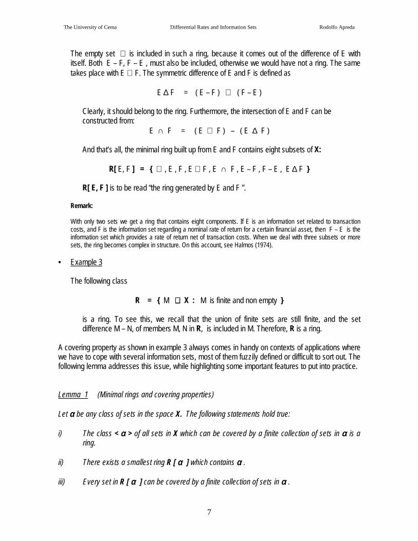
The empty set ∅ is included in such a ring, because it comes out of the difference of E withitself. Both E – F, F – E , must also be included, otherwise we would have not a ring. The sametakes place with E ∪ F. The symmetric difference of E and F is defined as

E ∆ F = ( E – F ) ∪ ( F – E )

Clearly, it should belong to the ring. Furthermore, the intersection of E and F can beconstructed from:

E ∩ F = ( E ∪ F ) – ( E ∆ F )

And that’s all, the minimal ring built up from E and F contains eight subsets of X:

R[ E, F ] = ∅ , E , F , E ∪ F , E ∩ F , E – F , F – E , E ∆ F

R[ E, F ] is to be read “the ring generated by E and F ”.

Remark:

With only two sets we get a ring that contains eight components. If E is an information set related to transactioncosts, and F is the information set regarding a nominal rate of return for a certain financial asset, then F – E is theinformation set which provides a rate of return net of transaction costs. When we deal with three subsets or moresets, the ring becomes complex in structure. On this account, see Halmos (1974).

• Example 3

The following class

R = M ⊆⊆⊆⊆ X : M is finite and non empty

is a ring. To see this, we recall that the union of finite sets are still finite, and the setdifference M – N, of members M, N in R, is included in M. Therefore, R is a ring.

A covering property as shown in example 3 always comes in handy on contexts of applications wherewe have to cope with several information sets, most of them fuzzily defined or difficult to sort out. Thefollowing lemma addresses this issue, while highlighting some important features to put into practice.

Lemma 1 (Minimal rings and covering properties)

Let αααα be any class of sets in the space X. The following statements hold true:

i) The class < αααα > of all sets in X which can be covered by a finite collection of sets in αααα is aring.

ii) There exists a smallest ring R [ αααα ] which contains αααα .

iii) Every set in R [ αααα ] can be covered by a finite collection of sets in αααα .


8

Proof: i) let us build up the following class of sets in X

< αααα > = M ⊆⊆⊆⊆ X : M ⊆⊆⊆⊆ ∪∪∪∪ 1 ≤≤≤≤ k ≤≤≤≤ N E k ; E k ∈∈∈∈ αααα

and take any M and any N in < αααα >.Then:

M ⊆⊆⊆⊆ ∪∪∪∪ 1 ≤≤≤≤ k ≤≤≤≤ N E k ; N ⊆⊆⊆⊆ ∪∪∪∪ 1 ≤≤≤≤ j ≤≤≤≤ M E j

it follows thatM ∪ N ⊆⊆⊆⊆ ∪∪∪∪ 1 ≤≤≤≤ v ≤≤≤≤ N + M E v ⇒⇒⇒⇒ M ∪ N ∈∈∈∈ < αααα >

Furthermore,M – N ⊆⊆⊆⊆ M ⊆⊆⊆⊆ ∪∪∪∪ 1 ≤≤≤≤ k ≤≤≤≤ N E k ⇒⇒⇒⇒ M – N ∈∈∈∈ < αααα >

Summing up, < αααα > is a ring.

ii) The set P( X ) of all subsets of X is a ring and the biggest one defined in X, then the class of sets ααααis contained at least by one ring. Let us take as R [ αααα ] the intersection of all the rings in X thatcontain αααα. It is certainly a ring, and it is contained in any ring which could contains αααα. Hence, R [ αααα ]is the smallest of all them; in other words, it is minimal.

iii) Let < αααα > be the class all of sets in X which can be covered by a finite union of sets in αααα. Inparticular, any set in αααα belongs to < αααα >. By i) < αααα > is a ring and by ii) it also contains the minimalring R [ αααα ] . χ

4.01.- APPLICATION OF LEMMA 1 TO INFORMATION SETS

a) For any family αααα of information sets, there exists a minimal ring which contains such family.

b) We usually meet a wide array of information sets, ranging from those with very few members, tothose families which contains even an infinite number of them. In a wider context of application, afamily of well-behaved information sets may available to the researcher but, on the other hand,she might be pursuing another family of information sets not so easy to reach. If the first familycan provide a covering feature, the second one would become more manageable eventually.

05.- ALGEBRAS OF SETS

Rings provide with a fairly good structure to deal with information sets. However, in many contexts ofanalysis and application, a stronger structure could perform even better. In fact, when we work onsome set in a ring, we are not granted that its complement belongs to the ring as well. As a ring doesnot usually contains the space X, we proceed to the concept of algebra of sets, which alwayscontains X.


9

Definition 2 Algebra of Sets

A is called an algebra of sets if it satisfies the following properties:

E ∈ A , F ∈ A ⇒⇒⇒⇒ E ∪ F ∈ A

E ∈ A , F ∈ A ⇒⇒⇒⇒ E C ∈ A

That is to say, an algebra of sets is an structure closed under unions and complements of sets. Someauthors, like Aliprantis (1999) or Halmos (1974), give a stylish translation of an algebra of sets asbeing any ring containing the space X.

• Example 4

The smallest algebra is the class ∅ , X , whereas the biggest one is the class P ( X ) of allsubsets of X. In fact, P ( X ) is closed under unions and complements, by definition. Hence, thereare two algebras in any space at least.

• Example 5

Let us take in X two different, non empty sets, E and F. We are going to construct the minimalalgebra that contains both sets. Firstly, it must contain X because is the complement of the emptyset. Also, the complements of E, F and E ∪ F must be in such algebra. There are other sets, andto show they should belong to the algebra, we take advantages of very well known set theoryproperties.

E ∩ F = ( E C ∪ F C ) C

( E – F ) = E ∩ F C ; ( F – E ) = E C ∩ F

E ∆ F = ( E – F ) ∪ ( F – E )

If these sets had to belong to the minimal algebra, so would their complements. All in all,there are sixteen sets in the minimal algebra that contains both E and F:

A = ∅ , X , E , F , E C , F C , E ∪ F , ( E ∪ F ) C , E ∩ F , ( E ∩ F ) C ,

( E – F ) , ( E – F ) C , ( F – E ) , ( F – E ) C , E ∆ F , ( E ∆ F ) C

With only two sets we get a ring that contains eight components. As an algebra grants thatcomplements remain within the structure, it comes as no surprise that the eight components ofthe ring in example 2 are present here, and their complements as well, so as to give sixteen setsin the algebra of sets.

An equivalent set of statements to those of Lemma 1 do not hold true for algebras. Nevertheless, wecan follow an easy transition from a ring to an algebra through next lemma, so as to proceed later to


10

another lemma which provides minimal algebras and covering features under somewhat restrictiveassumptions.

Lemma 2

If R is a ring in the space X, then the class of sets

A = M ⊆⊆⊆⊆ X : M ∈∈∈∈ R or M C ∈∈∈∈ R

is an algebra.

Proof: Firstly, let us take M ∈∈∈∈ A . There are two chances:

a) M = ( M C ) C ∈∈∈∈ R ⇒⇒⇒⇒ M C ∈∈∈∈ A

b) M C ∈∈∈∈ R ⇒⇒⇒⇒ M C ∈∈∈∈ A

Hence, for each set in A, its complement also belongs to A.

Secondly, suppose M , N are in A. There are three distinctive alternatives:

a) M , N ∈∈∈∈ R ⇒⇒⇒⇒ M ∪ N ∈∈∈∈ R ⇒⇒⇒⇒ M ∪ N ∈∈∈∈ A

b) M , N C ∈∈∈∈ R ⇒⇒⇒⇒ N C – M = N C ∩ M C = ( M ∪ N ) C ∈∈∈∈ R ⇒⇒⇒⇒ ( M ∪ N ) ∈∈∈∈ A

c) M C , N C ∈∈∈∈ R ⇒⇒⇒⇒ ( M C ∩ N C ) C = M ∪ N ∈∈∈∈ R ⇒⇒⇒⇒ M ∪ N ∈∈∈∈ A

In any case, ( M ∪ N ) ∈∈∈∈ A

Therefore, A qualifies as an algebra. χ

Remarks:

a) In many applications it could be helpful to know that some sets belong to one referential ring R and some otherssets, although not belonging to the benchmark ring, grant membership for their complements. Therefore, Lemma 2shows how both types of sets become members of a definite algebra eventually.

b) Example 3 could not be extended to an algebra whenever X is infinite.

For any family of well-behaved information sets we can generate a ring with covering properties asdepicted in Lemma 1. Whereas we can not extend those covering features to any algebra of setsoutright, next lemma will show that, with some qualifications, such extension can be reached anyway.


11

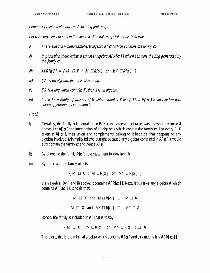
Lemma 3 ( minimal algebras and covering features)

Let αααα be any class of sets in the space X. The following statements hold true:

i) There exists a minimal (smallest) algebra A[ αααα ] which contains the family αααα.

ii) In particular, there exists a smallest algebra A[ R[αααα ] ] which contains the ring generated bythe family αααα.

iii) A[ R[αααα ] ] = M ⊆ X : M ∈ R[α ] or M C ∈ R[α ]

iv) If A is an algebra, then it is also a ring.

v) If R is a ring which contains X, then it is an algebra.

vi) Let αααα be a family of subsets of X which contains X itself. Then R[ αααα ] is an algebra withcovering features as in Lemma 1.

Proof:

i) Certainly, the family αααα is contained in P( X ), the largest algebra as was shown in example 4above. Let A[ αααα ] the intersection of all algebras which contain the family αααα. For every E, Ftaken in A[ αααα ], their union and complements belong to it because that happens to anyalgebra involved. Minimality follows outright because any algebra contained in A[ αααα ] it wouldalso contain the family αααα and hence A[ αααα ].

ii) By choosing the family R[αααα ] , the statement follows from i).

iii) By Lemma 2, the family of sets

M ⊆ X : M ∈ R[α ] or M C ∈ R[α ]

is an algebra. By i) and ii) above, it contains A[ R[αααα ] ]. Next, let us take any algebra A whichcontains A[ R[αααα ] ]. It holds that:

M ⊆ X and M ∈ R[α ] ⇒ M ∈ A

M ⊆ X and M C ∈ R[α ] ⇒ M C ∈ A

Hence, the family is included in A. That is to say:

M ⊆ X : M ∈ R[α ] or M C ∈ R[α ] ⊆ A

Therefore, this is the minimal algebra which contains R[ αααα ] and this means it is A[ R[ αααα ] ].


12

iv) Being an algebra, A is closed under unions. Besides, for every E, F in A,

E ∈ A , F ∈ A ⇒ E – F = E ∩ F C ∈ A . Hence, A is also a ring.

v) For every set E in the ring R, it follows

E C = X - E ∈ R

Hence, such a ring becomes an algebra.

vi) Let αααα be a family of subsets of X which contains X itself. By Lemma 1, R[ αααα ] is a ring withcovering features and it contains X. Besides, by v) it is an algebra. . χ

5.01.- APPLICATION OF LEMMA 3 TO INFORMATION SETS

a) For any family of information sets there exists a minimal algebra which contains αααα.

b) Furthermore, in many contexts of application, when we work on a family of feasible informationsets, it does not seem implausible to assume that X itself actually belongs to the family. In thatway, by means of Lemma 3 we can handle minimal algebras with covering features.

06.- DIFFERENTIAL RATES OF RETURN

Getting access to any information set could lead to finding out different sources which could explainthe rate of change r( t , T , ΩΩΩΩ t ) defined on the basic information set ΩΩΩΩ t and measured as in [02].What, for instance, if we knew that there is a subset ΩΩΩΩ1 t of ΩΩΩΩ t , namely,

ΩΩΩΩ 1 t ⊆⊆⊆⊆ ΩΩΩΩ t

which is so influential that could explain two thirds of the value of r( . ) at least? Let address twoexamples for this to happen. More applications, mainly in the financial markets context, can be foundin Apreda (2000b).

• Example 7

Assuming that we are about to value a financial asset and we know that the expected inflationrate will add one percentual point to the nominal rate of return for the period under analysis, hereΩΩΩΩ1 t accounts for the information set that deals with inflation data. It is for the remaining of thenominal r( . ) to track down transaction costs and the effective yield for the investor, exclusive ofinflation, and the information would be supplied by the difference between the basic set and ΩΩΩΩ1 t.


13

• Example 8

Let us suppose that we try to isolate variable costs attached to some measure of change, forinstance, profit rate per unit of a gadget to be sold. All the knowledge we need to calculate such acost component is gathered into ΩΩΩΩ1 t . It is for the remaining of the variable under study to trackdown fixed costs, semi-fixed costs, profits, and any other relevant item to the needs of theanalyst. Again, the information would be drawn from the difference

ΩΩΩΩ t – ΩΩΩΩ1 t

It is within this setting, as both Examples 7 and 8 have shown, that it becomes advisable to split downthe original rate of return into two components:

1 + r( t , T , ΩΩΩΩ t ) = [ 1 + s 1 ( t , T , ΩΩΩΩ 1 t ) ] . [ 1 + g 1 ( . ) ]

wheres 1 ( t , T , ΩΩΩΩ 1 t )

stands for the rate of change conditional to the information set ΩΩΩΩ1 t . Furthermore, g1( . ) comes upby solving the equation and stands for whatever remains of r( . ) after taking into account s1( . ). So,this complementary rate g1( . ) fills the gap between both rates and it is conditional upon theinformation set

ΩΩΩΩ t – ΩΩΩΩ 1 t

That means:g 1 ( . ) = g 1 ( t , T , ΩΩΩΩ t – ΩΩΩΩ 1 t )

Hence, we can now restate the former relationship between these three rates of change:

[04]1 + r( t , T , ΩΩΩΩ t ) = [ 1 + s 1 ( t , T , ΩΩΩΩ 1 t ) ] . [ 1 + g 1 ( t , T , ΩΩΩΩ t – ΩΩΩΩ 1 t ) ]

The discussion above has paved the way to the following definition. Although this definition keeps avery simple format lying on a general algebra of sets, we will proceed to uncover the underlyingstructure of such an algebra in section 06.01.

Definition 3: Simple Differential Rates on Residual Information Sets

Let A be an algebra of sets in X. Given the rates of return r( t , T , ΩΩΩΩ t ) and s 1( t , T , ΩΩΩΩ 1 t ) suchthat ΩΩΩΩ 1 t ⊆⊆⊆⊆ ΩΩΩΩ t , it is said that g 1( . ) is a simple differential rate to both r( . ) and s 1 ( . ) if andonly if

g 1( . ) = g 1 ( t , T , ΩΩΩΩ t – ΩΩΩΩ 1 t )and it fulfils:


14

1 + r( t , T , ΩΩΩΩ t ) = [ 1 + s 1 ( t , T , ΩΩΩΩ 1 t ) ] . [ 1 + g 1 ( t , T , ΩΩΩΩ t – ΩΩΩΩ 1 t ) ]

Furthermore, the set ΩΩΩΩ t – ΩΩΩΩ 1 t will be called a residual information set.

Remarks:

i) We see that g1 ( . ) is the remainder of the leading rate r( . ), given s1 ( . ).

ii) Residual sets come into light only because we have an underlying algebra which provides closure fordifferences. Although rings also allow such closure, oncoming developments will require complements to beused and, therefore, algebras become more flexible structures.

iii) When plugging numbers in definition 3, it may hold true that

[ 1 + s 1 ( t , T , ΩΩΩΩ 1 t ) ] . [ 1 + g 1 ( t , T , ΩΩΩΩ g t ) ] = [ 1 + s 1 ( t , T , ΩΩΩΩ 1 t ) ] . [ 1 + h 1 ( t , T , ΩΩΩΩ h t ) ]

which impliesg 1 ( t , T , ΩΩΩΩ g t ) = h 1 ( t , T , ΩΩΩΩ h t )

but this fact doesn’t convey that, as functions, g 1 ( . ) = h 1 ( . ) , because they can be defined on differentinformation sets.

iv) It is theformer remark that leads to a good reason for working with a cartesian product

R 1 x R 1 x A

as it is usual, for instance, in mathematical treatments on stochastic processes. (Oksendal, 1985)

What if we now tried to deal with g1 ( . ) the same way we did with r( . ), by resorting to the simpledifferential rates definition? That is to say, what if knew that we can pick out another rate s2 ( . )conditional upon the information set ΩΩΩΩ 2 t that fulfills:

ΩΩΩΩ 2 t ⊆⊆⊆⊆ ΩΩΩΩ t , ΩΩΩΩ 2 t ∩∩∩∩ ΩΩΩΩ 1 t ==== ∅∅∅∅

In that case we should ask for the remainder of g1 ( . ), and try to solve:

1 + g 1 ( t , T , ΩΩΩΩ t – ΩΩΩΩ 1 t ) = [ 1 + s 2 ( t , T , ΩΩΩΩ 2 t ) ] . [ 1 + g 2 ( . ) ]

Following this way, we may obtain a finite vector of rates of change

< s 1 ( . ) , s 2 ( . ) , ........ , s N ( . ) >

all of them stemming from the primary rate r( . ), and also a differential rate g N ( . ) performing as aremainder, so as the following relationship must hold true by iteration:

1 + r( t, T, ΩΩΩΩ t ) = ΠΠΠΠ 1 ≤≤≤≤ k ≤≤≤≤ N [ 1 + s k ( t, T, ΩΩΩΩ k t ) ] . [ 1 + g N ( . ) ]

Now, a problem certainly arises with this expression, because we have still said nothing on theunderlying information sets of the components in the following finite vector


15

< g 1 ( . ) , g 2 ( . ) , ........ , g N ( . ) >

To handle this difficulty, we need to enlarge upon Definition 2. Such a task will be accomplishedthrough two successive approaches. The first will lead to a narrower meaning of differential rate,whereas the second one will address an even broader but more realistic meaning, .

However, before expanding on what is understood by narrow and broad differential rates, we have toagree on the actual algebra of sets to be used as from now.

06.01.- CHOOSING THE RELEVANT ALGEBRA OF INFORMATION SETS

In practice, we choose a primary information set ΩΩΩΩ t in the space X, and we are concerned with acertain family of contextual sets in X, which might amount to economic variables or transaction costsstructures. It is the purpose of this section to show how a family of relevant sets may be spanned intoa suitable minimal algebra. An example will shed light about this sort of sets.

While dealing with financial assets rates of return, we should be intent on making the analysisinclusive of the transaction costs structure. At least, five contextual subsets of X seems to be useful(this approach has been developed in Apreda, 2000a and 2000b) :

• Intermediation costs : INT• Microstructure costs : MICR• Financial costs on transactions : FIN• Information costs : INF• Taxes : TAX

We define a family of contextual sets to ΩΩΩΩ t :

αααα = E , F , G , H , J , where

E = Ω t ∩ INT ; F = Ω t ∩ MICR ; G = Ω t ∩ FIN ; H = Ω t ∩ INF ; J = Ω t ∩ TAX

The minimal algebra which is spanned by these sets and ΩΩΩΩ t. will meet our purposes. We denote thisalgebra as A[ ΩΩΩΩ t , αααα ] . That is to say:

A[ ΩΩΩΩ t , αααα ] = A [ E, F, G, H, J, ΩΩΩΩ t ]

If we want to go beyond transaction costs, the class could be embedded into a larger one, with morefactors of analysis. For instance, inflation, rate of exchange, and so on. Making for a definition, weget:

Definition 4: The relevant algebra for information sets

Given ΩΩΩΩ t ⊆⊆⊆⊆ X , and a finite family of sets in X ,


16

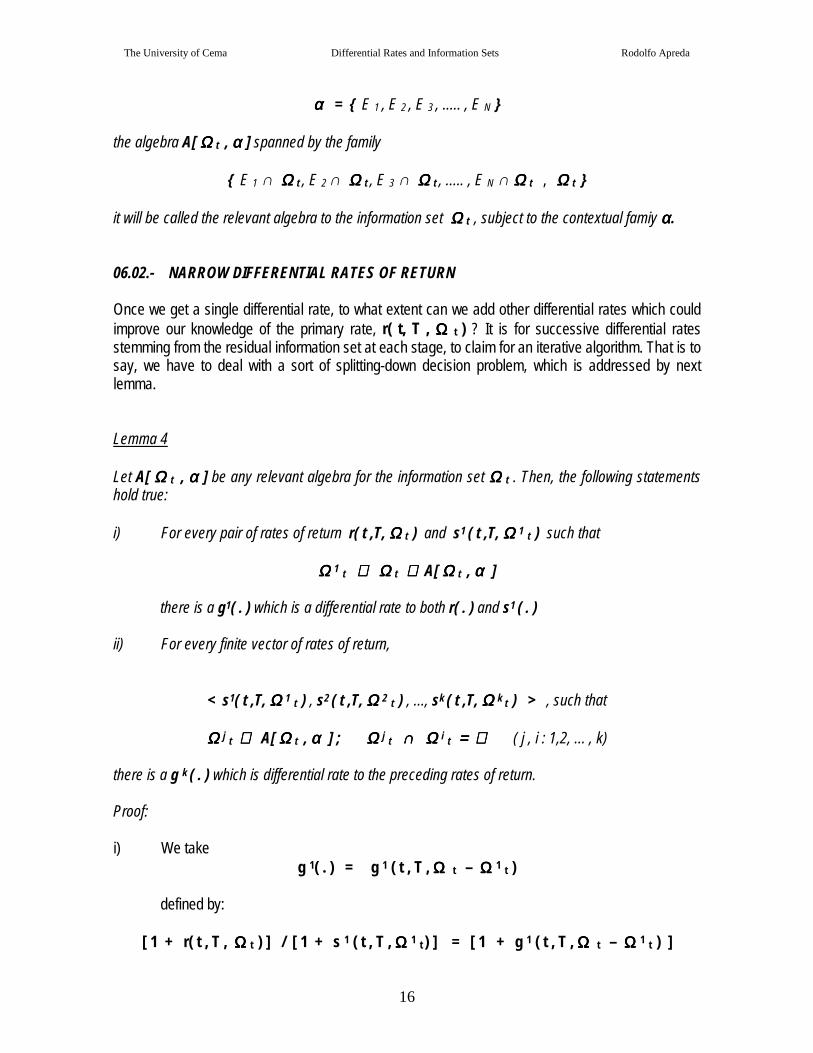
αααα = E 1 , E 2 , E 3 , ..... , E N

the algebra A[ ΩΩΩΩ t , αααα ] spanned by the family

E 1 ∩ ΩΩΩΩ t , E 2 ∩ ΩΩΩΩ t , E 3 ∩ ΩΩΩΩ t , ..... , E N ∩ ΩΩΩΩ t , ΩΩΩΩ t

it will be called the relevant algebra to the information set ΩΩΩΩ t , subject to the contextual famiy αααα.

06.02.- NARROW DIFFERENTIAL RATES OF RETURN

Once we get a single differential rate, to what extent can we add other differential rates which couldimprove our knowledge of the primary rate, r( t, T , ΩΩΩΩ t ) ? It is for successive differential ratesstemming from the residual information set at each stage, to claim for an iterative algorithm. That is tosay, we have to deal with a sort of splitting-down decision problem, which is addressed by nextlemma.

Lemma 4

Let A[ ΩΩΩΩ t , αααα ] be any relevant algebra for the information set ΩΩΩΩ t . Then, the following statementshold true:

i) For every pair of rates of return r( t ,T, ΩΩΩΩ t ) and s1 ( t ,T, ΩΩΩΩ 1 t ) such that

ΩΩΩΩ 1 t ⊆⊆⊆⊆ ΩΩΩΩ t ∈∈∈∈ A[ ΩΩΩΩ t , αααα ]

there is a g1( . ) which is a differential rate to both r( . ) and s1 ( . )

ii) For every finite vector of rates of return,

< s1( t ,T, ΩΩΩΩ 1 t ) , s2 ( t ,T, ΩΩΩΩ 2 t ) , ..., sk ( t ,T, ΩΩΩΩ k t ) > , such that

ΩΩΩΩ j t ∈∈∈∈ A[ ΩΩΩΩ t , αααα ] ; ΩΩΩΩ j t ∩∩∩∩ ΩΩΩΩ i t ==== ∅∅∅∅ ( j , i : 1,2, ... , k)

there is a g k ( . ) which is differential rate to the preceding rates of return.

Proof:

i) We takeg 1( . ) = g 1 ( t , T , ΩΩΩΩ t – ΩΩΩΩ 1 t )

defined by:

[ 1 + r( t , T , ΩΩΩΩ t ) ] / [ 1 + s 1 ( t , T , ΩΩΩΩ 1 t ) ] = [ 1 + g 1 ( t , T , ΩΩΩΩ t – ΩΩΩΩ 1 t ) ]


17

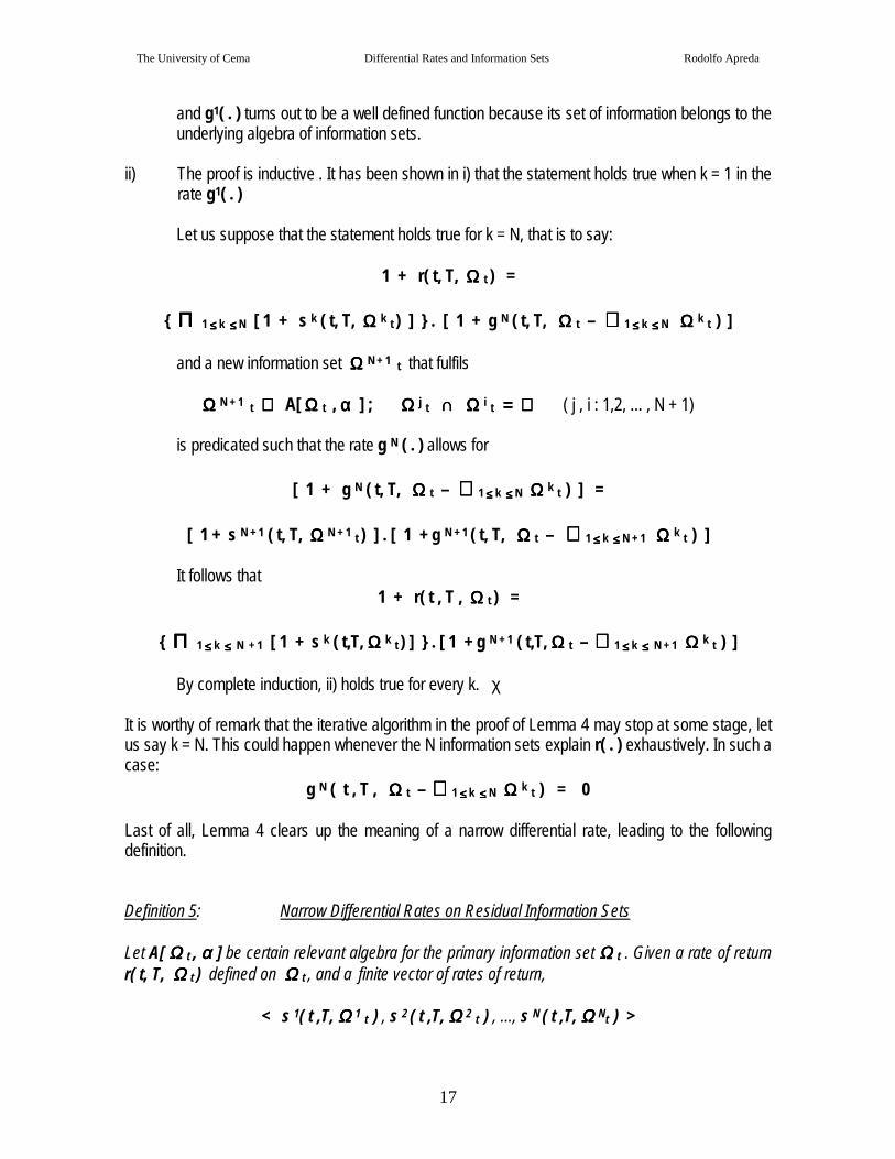
and g1( . ) turns out to be a well defined function because its set of information belongs to theunderlying algebra of information sets.

ii) The proof is inductive . It has been shown in i) that the statement holds true when k = 1 in therate g1( . )

Let us suppose that the statement holds true for k = N, that is to say:

1 + r( t, T, ΩΩΩΩ t ) =

ΠΠΠΠ 1 ≤≤≤≤ k ≤≤≤≤ N [ 1 + s k ( t, T, ΩΩΩΩ k t ) ] . [ 1 + g N ( t, T, ΩΩΩΩ t – ∪∪∪∪ 1 ≤≤≤≤ k ≤≤≤≤ N ΩΩΩΩ k t ) ]

and a new information set ΩΩΩΩ N + 1 t that fulfils

ΩΩΩΩ N + 1 t ∈∈∈∈ A[ ΩΩΩΩ t , αααα ] ; ΩΩΩΩ j t ∩∩∩∩ ΩΩΩΩ i t ==== ∅∅∅∅ ( j , i : 1,2, ... , N + 1)

is predicated such that the rate g N ( . ) allows for

[ 1 + g N ( t, T, ΩΩΩΩ t – ∪∪∪∪ 1 ≤≤≤≤ k ≤≤≤≤ N ΩΩΩΩ k t ) ] =

[ 1 + s N + 1 ( t, T, ΩΩΩΩ N + 1 t ) ] . [ 1 + g N + 1 ( t, T, ΩΩΩΩ t – ∪∪∪∪ 1 ≤≤≤≤ k ≤≤≤≤ N + 1 ΩΩΩΩ k t ) ]

It follows that1 + r( t , T , ΩΩΩΩ t ) =

ΠΠΠΠ 1 ≤≤≤≤ k ≤≤≤≤ N + 1 [ 1 + s k ( t,T, ΩΩΩΩ k t ) ] . [ 1 + g N + 1 ( t,T, ΩΩΩΩ t – ∪∪∪∪ 1 ≤≤≤≤ k ≤≤≤≤ N + 1 ΩΩΩΩ k t ) ]

By complete induction, ii) holds true for every k. χ

It is worthy of remark that the iterative algorithm in the proof of Lemma 4 may stop at some stage, letus say k = N. This could happen whenever the N information sets explain r( . ) exhaustively. In such acase:

g N ( t , T , ΩΩΩΩ t – ∪∪∪∪ 1 ≤≤≤≤ k ≤≤≤≤ N ΩΩΩΩ k t ) = 0

Last of all, Lemma 4 clears up the meaning of a narrow differential rate, leading to the followingdefinition.

Definition 5: Narrow Differential Rates on Residual Information Sets

Let A[ ΩΩΩΩ t , αααα ] be certain relevant algebra for the primary information set ΩΩΩΩ t . Given a rate of returnr( t, T, ΩΩΩΩ t ) defined on ΩΩΩΩ t , and a finite vector of rates of return,

< s 1( t ,T, ΩΩΩΩ 1 t ) , s 2 ( t ,T, ΩΩΩΩ 2 t ) , ..., s N ( t ,T, ΩΩΩΩ Nt ) >


18

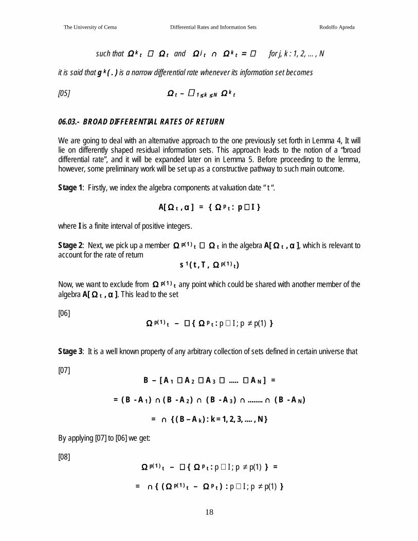
such that ΩΩΩΩ k t ⊆⊆⊆⊆ ΩΩΩΩ t and ΩΩΩΩ j t ∩∩∩∩ ΩΩΩΩ k t ==== ∅∅∅∅ for j, k : 1, 2, ... , N

it is said that g k ( . ) is a narrow differential rate whenever its information set becomes

[05] ΩΩΩΩ t – ∪∪∪∪ 1 ≤≤≤≤ k ≤≤≤≤ N ΩΩΩΩ k t

06.03.- BROAD DIFFERENTIAL RATES OF RETURN

We are going to deal with an alternative approach to the one previously set forth in Lemma 4, It willlie on differently shaped residual information sets. This approach leads to the notion of a “broaddifferential rate”, and it will be expanded later on in Lemma 5. Before proceeding to the lemma,however, some preliminary work will be set up as a constructive pathway to such main outcome.

Stage 1: Firstly, we index the algebra components at valuation date “ t “.

A[ ΩΩΩΩ t , αααα ] = ΩΩΩΩ p t : p ∈∈∈∈ I

where I is a finite interval of positive integers.

Stage 2: Next, we pick up a member ΩΩΩΩ p( 1 ) t ⊆⊆⊆⊆ ΩΩΩΩ t in the algebra A[ ΩΩΩΩ t , αααα ], which is relevant toaccount for the rate of return

s 1 ( t , T , ΩΩΩΩ p( 1 ) t )

Now, we want to exclude from ΩΩΩΩ p( 1 ) t any point which could be shared with another member of thealgebra A[ ΩΩΩΩ t , αααα ]. This lead to the set

[06]ΩΩΩΩ p( 1 ) t – ∪∪∪∪ ΩΩΩΩ p t : p ∈ I ; p ≠ p(1)

Stage 3: It is a well known property of any arbitrary collection of sets defined in certain universe that

[07]B – [ A 1 ∪∪∪∪ A 2 ∪∪∪∪ A 3 ∪∪∪∪ ..... ∪∪∪∪ A N ] =

= ( B - A 1 ) ∩∩∩∩ ( B - A 2 ) ∩∩∩∩ ( B - A 3 ) ∩∩∩∩ ........ ∩∩∩∩ ( B - A N )

= ∩∩∩∩ ( B – A k ) : k = 1, 2, 3, .... , N

By applying [07] to [06] we get:

[08]ΩΩΩΩ p( 1 ) t – ∪∪∪∪ ΩΩΩΩ p t : p ∈ I ; p ≠ p(1) =

= ∩∩∩∩ ( ΩΩΩΩ p( 1 ) t – ΩΩΩΩ p t ) : p ∈ I ; p ≠ p(1)


19

Stage 4 : In the equation

1 + r( t , T , ΩΩΩΩ t ) = [ 1 + s 1 ( t , T , ΩΩΩΩ p( 1 ) t ) ] . [ 1 + g 1 ( . ) ]

and taking advantage of [08], we will choose as the underlying residual information set for g1 ( . )

[09]ΩΩΩΩ t – ∩∩∩∩ ( ΩΩΩΩ p( 1 ) t – ΩΩΩΩ p t ) : p ∈ I ; p ≠ p(1)

This set brings back all the elements in ΩΩΩΩ p( 1 ) t which could be of interest for any other informationset relevant to following differential rates. That is to say, g1 ( . ) is defined on all the points of ΩΩΩΩ tincluding those points in the sets overlapping with ΩΩΩΩ p( 1 ) t .

Stage 5 : We labour [09] by means of properties that hold for arbitrary collections of sets, namely:

ΩΩΩΩ t – ∩∩∩∩ ( ΩΩΩΩ p( 1 ) t – ΩΩΩΩ p t ) : p ∈ I ; p ≠ p(1) =

= ΩΩΩΩ t ∩∩∩∩ < ∩∩∩∩ ( ΩΩΩΩ p( 1 ) t – ΩΩΩΩ p t ) : p ∈ I ; p ≠ p(1) > C

= ΩΩΩΩ t ∩∩∩∩ < ∪∪∪∪ ( ΩΩΩΩ p( 1 ) t – ΩΩΩΩ p t ) C : p ∈ I ; p ≠ p(1) >

= ΩΩΩΩ t ∩∩∩∩ < ∪∪∪∪ ( ΩΩΩΩ p( 1 ) t ∩∩∩∩ ( ΩΩΩΩ p t ) C ) C : p ∈ I ; p ≠ p(1) >

= ΩΩΩΩ t ∩∩∩∩ < ∪∪∪∪ ( ( ΩΩΩΩ p( 1 ) t ) C ∪∪∪∪ ΩΩΩΩ p t ) : p ∈ I ; p ≠ p(1) >

= < ΩΩΩΩ t ∩∩∩∩ (ΩΩΩΩ p( 1 ) t ) C > ∪∪∪∪ < ∪∪∪∪ ( ΩΩΩΩ t ∩∩∩∩ ΩΩΩΩ p t ) : p ∈ I ; p ≠ p(1) >

= < ΩΩΩΩ t – ΩΩΩΩ p( 1 ) t > ∪∪∪∪ < ∪∪∪∪ ( ΩΩΩΩ t ∩∩∩∩ ΩΩΩΩ p t ) : p ∈ I ; p ≠ p(1) >

Summing up, the residual information set for g1 ( . ) will be:

[10]ΩΩΩΩ t – ∩∩∩∩ ( ΩΩΩΩ p( 1 ) t – ΩΩΩΩ p t ) : p ∈ I ; p ≠ p(1) =


This relationship is worthy of remark:

(a) The first part of it, namely

< ΩΩΩΩ t – ΩΩΩΩ p( 1 ) t >

is the same as in [05], that is to say, the residual set we set up in the narrow approach to differentialrates.

(b) The second part of it, namely


20

< ∪∪∪∪ ( ΩΩΩΩ t ∩∩∩∩ ΩΩΩΩ p t ) : p ∈ I ; p ≠ p(1) >

conveys the sharing of information with all overlapping sets, as stand-by remainders to be used byother differential rates. As we see, residual sets are not so restrictive here as they were in the narrowapproach to differential rates.

Stage 6 : At this stage, we are going to pick another member of A[ ΩΩΩΩ t , αααα ],

ΩΩΩΩ p( 2 ) t ⊆⊆⊆⊆ ΩΩΩΩ t ,

which is relevant to account for the rate of return

s2 ( t , T , ΩΩΩΩ p( 2 ) t )

Up to this point, we would like to isolate from ΩΩΩΩ p( 2 ) t any point which could be shared with anothermember of A[ ΩΩΩΩ t , αααα ] eventually. As we are in the second rate of return, another ΩΩΩΩ p( 1 ) t has beenpreviously taken into account. So, we want to isolate from

ΩΩΩΩ p( 1 ) t ∪∪∪∪ ΩΩΩΩ p( 2 ) t

any point which could be shared with another member of A[ ΩΩΩΩ t , αααα ]. This leads to the set

( ΩΩΩΩ p( 1 ) t ∪∪∪∪ ΩΩΩΩ p( 2 ) t ) – ∪∪∪∪ ΩΩΩΩ p t : p ∈ I ; p ≠ p(1) , p(2)

By using [07] this set can also be translated as

( ΩΩΩΩ p( 1 ) t ∪∪∪∪ ΩΩΩΩ p( 2 ) t ) – ∪∪∪∪ ΩΩΩΩ p t : p ∈ I ; p ≠ p(1) , p(2) =

= ∩∩∩∩ [ ( ΩΩΩΩ p( 1 ) t ∪∪∪∪ ΩΩΩΩ p( 2 ) t ) – ΩΩΩΩ p t ] : p ∈ I ; p ≠ p(1) , p(2)

Stage 7 : Next, we have to solve for the new differential rate, as we did in stage 4:

1 + g 1 ( . ) = [ 1 + s 2 ( t , T , ΩΩΩΩ p( 2 ) t ) ] . [ 1 + g 2 ( . ) ]

and we proceed to choose the residual information set of g2 ( . )

[12]ΩΩΩΩ t – ∩∩∩∩ [ ( ΩΩΩΩ p( 1 ) t ∪∪∪∪ ΩΩΩΩ p( 2 ) t ) – ΩΩΩΩ p t ] : p ∈ I ; p ≠ p(1) , p(2)

This set brings back all the elements in (ΩΩΩΩ p( 1 ) t ∪∪∪∪ ΩΩΩΩ p( 2 ) t ) which could be of interest for any otherinformation set relevant to the following differential rates. That is to say, g2 ( . ) is defined on all thepoints of ΩΩΩΩ t including those points in the sets overlapping with

(ΩΩΩΩ p( 1 ) t ∪∪∪∪ ΩΩΩΩ p( 2 ) t ).

we get a working expression of [12] , through the same steps we did in stage 5:


21

[13]ΩΩΩΩ t – ∩∩∩∩ [ ( ΩΩΩΩ p( 1 ) t ∪∪∪∪ ΩΩΩΩ p( 2 ) t ) – ΩΩΩΩ p t ] : p ∈ I ; p ≠ p(1) , p(2) =

= < ΩΩΩΩ t – ( ΩΩΩΩ p( 1 ) t ∪∪∪∪ ΩΩΩΩ p( 2 ) t ) > ∪∪∪∪ < ∪∪∪∪ ( ΩΩΩΩ t ∩∩∩∩ ΩΩΩΩ p t ) : p ∈ I ; p ≠ p(1) , p(2) >

It should not come as a surprise that the first part in the last expresion, namely:

< ΩΩΩΩ t – ( ΩΩΩΩ p( 1 ) t ∪∪∪∪ ΩΩΩΩ p( 2 ) t ) >

is the same as in [5], that is to say the same residual set used in the narrow approach to differentialrates. On the other hand, the second part in the last expression amounts to

< ∪∪∪∪ ( ΩΩΩΩ t ∩∩∩∩ ΩΩΩΩ p t ) : p ∈ I ; p ≠ p(1) , p(2) >

it conveys information sharing with overlapping sets, as stand-by remainders to be used by otherdifferential rates.

Taking advantage of this rather lengthy discussion, next lemma can be easily set forth.

Lemma 5

Let A[ ΩΩΩΩ t , αααα ] be the relevant algebra to the information set ΩΩΩΩ t , indexed by a finite interval I ofpositive integers,


Then, the following statements hold true:

i) For every pair of rates of return r( t ,T, ΩΩΩΩ t ) and s 1 ( t ,T, ΩΩΩΩ 1 t ) such that

ΩΩΩΩ 1 t ⊆⊆⊆⊆ ΩΩΩΩ t ∈∈∈∈ A[ ΩΩΩΩ t , αααα ]

there is one g1( . ) which is a differential rate to both r( . ) and s1 ( . )

ii) For every finite vector of rates of return,

< s1( t ,T, ΩΩΩΩ 1 t ) , s2 ( t ,T, ΩΩΩΩ 2 t ) , ..., sk ( t ,T, ΩΩΩΩ k t ) >

such that ΩΩΩΩ j t ∈∈∈∈ A[ ΩΩΩΩ t , αααα ] ( j : 1,2, ... , k)

there is one gk ( . ) which is differential rate to the preceding rates of return.

Proof:

We are going to proceed by induction on k. If k = 1 , then we use stages 1 to 5 from the previousdiscussion. In fact, from [11] we have:


22

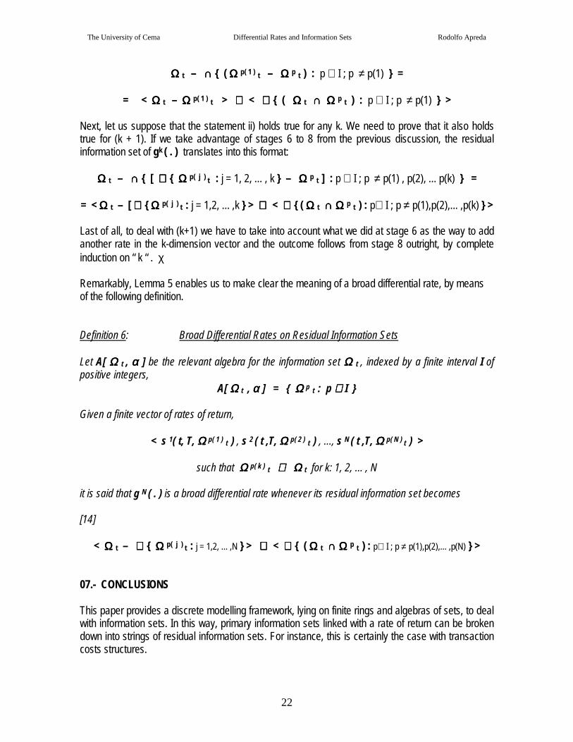
ΩΩΩΩ t – ∩∩∩∩ ( ΩΩΩΩ p( 1 ) t – ΩΩΩΩ p t ) : p ∈ I ; p ≠ p(1) =


Next, let us suppose that the statement ii) holds true for any k. We need to prove that it also holdstrue for (k + 1). If we take advantage of stages 6 to 8 from the previous discussion, the residualinformation set of gk ( . ) translates into this format:

ΩΩΩΩ t – ∩∩∩∩ [ ∪∪∪∪ ΩΩΩΩ p( j ) t : j = 1, 2, ... , k – ΩΩΩΩ p t ] : p ∈ I ; p ≠ p(1) , p(2), ... p(k) =

= < ΩΩΩΩ t – [ ∪∪∪∪ ΩΩΩΩ p( j ) t : j = 1,2, ... ,k > ∪∪∪∪ < ∪∪∪∪ ( ΩΩΩΩ t ∩∩∩∩ ΩΩΩΩ p t ) : p∈ I ; p ≠ p(1),p(2),... ,p(k) >

Last of all, to deal with (k+1) we have to take into account what we did at stage 6 as the way to addanother rate in the k-dimension vector and the outcome follows from stage 8 outright, by completeinduction on “ k “ . χ

Remarkably, Lemma 5 enables us to make clear the meaning of a broad differential rate, by meansof the following definition.

Definition 6: Broad Differential Rates on Residual Information Sets

Let A[ ΩΩΩΩ t , αααα ] be the relevant algebra for the information set ΩΩΩΩ t , indexed by a finite interval I ofpositive integers,


Given a finite vector of rates of return,

< s 1( t, T, ΩΩΩΩ p( 1 ) t ) , s 2 ( t ,T, ΩΩΩΩ p( 2 ) t ) , ..., s N ( t ,T, ΩΩΩΩ p( N ) t ) >

such that ΩΩΩΩ p( k ) t ⊆⊆⊆⊆ ΩΩΩΩ t for k: 1, 2, ... , N

it is said that g N ( . ) is a broad differential rate whenever its residual information set becomes

[14]

< ΩΩΩΩ t – ∪∪∪∪ ΩΩΩΩ p( j ) t : j = 1,2, ... ,N > ∪∪∪∪ < ∪∪∪∪ ( ΩΩΩΩ t ∩∩∩∩ ΩΩΩΩ p t ) : p∈ I ; p ≠ p(1),p(2),... ,p(N) >

07.- CONCLUSIONS

This paper provides a discrete modelling framework, lying on finite rings and algebras of sets, to dealwith information sets. In this way, primary information sets linked with a rate of return can be brokendown into strings of residual information sets. For instance, this is certainly the case with transactioncosts structures.


23

The main contributions can be found in section 06, where two lemmas are proved. The first onemakes possible the use of differential rates of return with restrictive assumptions on their informationsets, as most customary applications seem to have need of. The second lemma attempts to get abroader outcome, so as to cope with differential rates lying on realistic residual information sets.Lastly, both lemmas pave the way to definitions of narrow and broad differential rates as residualinformation sets.

REFERENCES

Aliprantis, C. and Border, K. (1999). Infinite Dimensional Analysis. Springer-Verlag, second edition, New York.

Apreda, R.. (1999a). Transactionally Efficient Markets, Dynamic Arbitrage and Microstructure.Working Paper Series N°151, Universidad del Cema, Buenos Aires.

Apreda, R.. (1999b). Dynamic Arbitrage Gaps for Financial Assets in a Nonlinear and Chaotic Adjustment Price Process.Journal of Multinational Financial Managament, volume 9, pp. 441-457.

Apreda, R. (2000a). A Transaction Costs Approach to Financial Assets Rates of Return. Working Paper Series N° 161,Universidad del Cema, Buenos Aires.

Apreda, R.( 2000b). Differential Rates and Information Sets: A toolkit for Practitioners, Financial Economists andAccountants. Working Paper Series N° 166, Universidad del Cema, Buenos Aires.

Apreda, R.( 2000c). Information Sets and the Brokerage of Asymmetric Information. Working Paper Series, forthcoming inDecember, Universidad del Cema, Buenos Aires.

Berge, C. (1997). Topological Spaces. Dover, New York.

Cuthbertson, K. (1996). Quantitative Financial Economics. J. Wiley, New York.

Daniel, K. and Titman, S. (2000). Market Efficiency in an Irrational World. NBER, Working Paper 7489.

Day, R. (1994). Complex Economics Dynamics. Volume 1: An Introduction to Dynamical Systems and MarketMechanisms. The Mit Press, Massachusetts.

Dotham, M. (1990). Prices in Financial Assets. Oxford University Press, New York.

Elton, J. (1999). Expected Returns, Realized Returns, and Asset Pricing Tests. Journal of Finance, vol. 54, n° 4, pp.1199-1220.

Elton, J. and Gruber, M. (1995). Modern Portlolio Analysis and Investment Theory.John Wiley, New York.

Fama, E. (1970). Efficient Capital Markets: A Review of Theory and Empirical Work. Journal of Finance, vol.25, n°2, pp.383-417

Fama, E. (1991). Efficient Capital Markets II. Journal of Finance, vol. 46, pp. 1575-1617

Gonedes, N. (1975). Information-Production and Capital Market Equilibrium. Journal of Finance, vol. 30, n°3, pp. 841-864.

Gonedes, N. (1976). The Capital Market, the Market for Information, and External Accounting. Journal of Finance, vol. 31,n° 2, pp. 611-630.


24

Grossman, S. and Stiglitz, J. (1980). On the Impossibility of Informationally Efficient Markets. American EconomicReview.

Halmos, P. (1974). Measure Theory. Springer-Verlag, New York

Halmos, P. and Givant, S. (1998). Logic as Algebra. Dolciani Mathematical Exposition N° 21, The MathematicalAssociation of America.

Hart, O. (1995). Firms, Contracts and Financial Structure. Clarendon Lectures in Economics, Oxford University Press,Oxford.

Hubbard, J. and Hubbard, B. (1999). Vector Calculus, Linear Algebra and Differential Forms: A Unified Approach.Prentice Hall, New Jersey.

Itô, K. (1995). A Survey of Stochastic Differential Equations. Included in Non Linear and Convex Analysis in EconomicTheory, by Maruyama T. and Takahashi, W. (Editors). Springer, Berlin, New York.

Oksendal, B. (1985). Stochastic Differential Equations. Springer, Berlin.

Rasmusen, E. (1994). Games and Information. Blackwell, second edition, Massachusetts.

Shleifer, A. (1999). Inefficient Markets. Oxford University Press, Oxford.

Williamson, O. (1996). The Mechanisms of Governance. Oxford University Press, New York.


25

APPENDIX

Given a space or universe X, non empty, a subset E of X will be defined as a set such that:

( ∀ x ) : x ∈ E ⇒ x ∈ X

The set built up with all the subsets of X will be denoted as P(X) and it comes defined as:

P(X) = A : A ⊆ X

When dealing with sets of sets, it is rather preferred to speak about families of sets. Then, P(X) is afamily of sets. Let us take two arbitrary subsets A and B in X. The following operations between thembuild up new sets.

Union of two sets:A ∪∪∪∪ B = x : x ∈ A or x ∈ B

Intersection of two sets:A ∩∩∩∩ B = x : x ∈ A and x ∈ B

Difference of two sets:A – B = x : x ∈ A and x ∉ B

Symmetric difference of two sets:

A ∆∆∆∆ B = x : x ∈ A – B or x ∈ B – A

Complement of a set:A C = x : x ∉ A

Family of sets:

A family, or class, of sets in the space X, indexed by the index set I, is a function

F : I →→→→ X

Usually, the family is written: A λλλλ : λλλλ ∈∈∈∈ I

The members in the family are the sets A λλλλ = F (λ)

• For an excellent introduction to logic, from an algebraic perspective, is highly remarkable the latest book by Halmos-Givant (1998).

• Very useful books on advanced mathematics, both suitable for economists and financial economics with goodmathematics background, are Aliprantis and Border (1999), and Berge’s book on topological spaces. (Berge, 1997).

differential rates of return and residual

Documents