differential scanning calorimeter analysis of hydrino ...differential scanning calorimeter analysis...
TRANSCRIPT
Differential Scanning Calorimeter Analysis of Hydrino-Producing Solid Fuel
Dr. Gilbert L. Crouse, Jr.1
Introduction A new theory of electron behavior in the atom has been developed in the last two decades by Mills [1] and is a departure from the traditional quantum mechanics (QM) model of the atom. The Schrödinger equation forms the foundation for the QM model of electron behavior in the atom but does not come from first principles and implies that the classical laws of physics are not applicable at the atomic scale. Mills’ classical physics (CP) approach is so named because it starts with the classical laws of physics, Maxwell’s equations, Newton’s laws, etc, and applies those laws at the atomic level. The foundation of Mills’ electron model is the observation that atoms in their ground state do not radiate an electromagnetic (EM) field. If an atom were to radiate an EM field it would continually loose energy and it would not be stable which is clearly not the case for atoms in their ground state. This is significant because an atom’s electrons “orbit” the nucleus of the atom in some way and hence they are in a continual state of acceleration as they orbit. From classical EM theory it is known that a charged particle undergoing acceleration usually radiates an EM field. Since the electrons do not radiate, we have a key boundary condition on the electron’s motion. Haus [2] solved the condition whereby charged particles radiate an EM field and determined that only the Fourier components synchronous with the speed of light contribute to the charged particle’s field. Mills used the inverse of this observation, i.e. that motion without Fourier components synchronous with the speed of light does not result in a radiated field, as a framework for determining a representation of the electron that obeys the nonradiative boundary condition. Mills then derived an atomic model that unlike the Schrödinger equation approach obeys first principles and directly models the concepts of spin and excited states. The approach has proven very useful in chemistry applications allowing much more accurate calculations of binding energies for a wide variety of compounds than any previous theoretical method.
Perhaps the most exciting and practical implication of Mills’ theory is the prediction of what is being called the Hydrino. CP as well as QM predict integral quantum number excited states of atoms. These excited states are well known and experimentally verified. However, CP also predicts the existence of fractional quantum states and specifically for the hydrogen atom it predicts that these lower energy states are stable. These fractional states have lower energy that the normal ground state of the hydrogen atom and Mills has coined the term “hydrino” for a hydrogen atom in one of these lower energy states. This result implies that if hydrogen atoms can be induced to transition from their ground 1 This research was performed while the author was an Associate Professor of Aerospace Engineering at Auburn University, Auburn, AL

state to one of the hydrino states, then the transition would be accompanied by a rather large release of energy. Moreover, this energy release could be a very significant and economical source of power.
Since the development of the CP theory, Mills and his company Blacklight Power have been experimenting with methods for demonstrating and harnessing this energy source. Their research has determined that hydrogen atoms can be induced to transition into hydrino states when brought into contact with other atoms or molecules that can accept the correct amount of energy. One of the methods found for demonstrating the transition is to mix Cu(OH)2 and CuBr2 in a pressure vessel and heat to 150-200 °C [3]. When Cu(OH)2 is heated by itself to that range it will decompose into CuO and H2O absorbing energy during the reaction. On the other hand CuBr2 by itself does not undergo any phase transitions or reactions in that temperature range. In contrast, the mixture of the two exhibits a strong exothermal reaction in that temperature range in Mills’ experiment [3]. Since this energy release is not explained by conventional chemistry and predicted spectroscopic signatures indicating the presence of hydrinos are observed on the products, Mills’ conclusion is that the experiment provides a clear demonstration of the hydrogen to hydrino transition predicted by CP theory. This paper documents independent replication of Mills’ experiment.
Description of Experiment The energy release when the Cu(OH)2 and CuBr2 mixture is heated was measured here using a differential scanning calorimeter (DSC). A DSC measures the amount of heat needed to change the temperature of a sample through a temperature range. Two identical metal pans, one containing the sample and one empty as a reference, are placed in a precisely calibrated furnace and the amount of heat added to each pan is carefully measured as the furnace is heated and cooled. By looking at the difference between the two pans, the heat required to change the temperature of the sample can be isolated. This apparatus can be used to study heat capacity, heat of fusion, or endothermic/exothermic reactions for example.
For this study a TA Instruments Q2000 DSC machine was used [4]. Typically small aluminum pans which may or may not be hermetically sealed are used as the sample containers. In this experiment however, the samples release gases when heated so sealed, stainless steel containers were used. The pans used, PerkinElmer part number B0182901 [5] and shown below, had screw-on lids and gold-plated copper seals to allow internal pressures up to 150 atmospheres. These pans were purchased from Thermal Support, Inc. [6] directly by Auburn University. As will be discussed these pans were significantly heavier than the typical aluminum pans so a special calibration was required to obtain accurate results.
2

Figure 1. PerkinElmer high pressure capsules [5] and TA Q2000 DSC [4]
During testing, two pans were used. One pan served as the reference and was empty. The second pan contained the sample. For each run, the following temperature sequence was used.
1. Equilibrate the two pans at 40 °C2. Hold the temperature of 40 °C for one minute3. Ramp the temperature to 300 °C at 5 °C/min4. Equilibrate the two pans at 300 °C5. Ramp the temperature to 40 °C at 10 °C/min
Sample Preparation The reagents for this experiment were Copper(II) Hydroxide and Copper(II) Bromide. These were obtained from Sigma-Aldrich directly by Auburn University as follows
Compound Part # Description Cu(OH)2 289787 Copper(II) hydroxide, technical grade [7] CuBr2 437867 Copper(II) bromide, 99.999% trace metals basis [8]
The assumed reaction for the experiment was
2Cu(OH)2 + 2CuBr2 → H2O + 2CuBr2 + 2CuO + 1/2O2 + 2H(1/4) + heat
where H(1/4) refers to hydrogen in the ¼ hydrino state. Since equal molar quantities of the two reagents are needed for this assumed reaction, the two reagents were mixed in proportion to their molecular weights. 188.70 mg of CuBr2 and 82.23 mg of Cu(OH)2 were mixed and stored in a glass vial for the DSC tests. The reagents were measured on a Mettler Toledo XS205 Dual Range Analytical Balance which reads to 0.01 mg. Once measured the chemicals were mixed on a flat surface with a stainless steel spatula. The same balance was used to weigh all samples.
The stainless steel sample pans were designed to be reused. Between DSC runs the sample pan was cleaned using a cotton swab and acetone followed by an acetone rinse. A fresh gold-plated copper seal was used for each run. The sample pan and seal were weighed using the balance to determine the
3
container weight. The sample was then placed in the container and the combination weighed again using the balance. The lid of the container was then screwed on to seal the container. The sample weight was determined by subtracting the empty container weight from the total weight of the filled container. Typically 10-20 mg of material were used for each run. This is more than recommended for standard aluminum pans but the larger sample size was used because of the large mass of the stainless steel pressure capsules (600+ mg versus 40-50 mg for aluminum).
Note that in contrast to the work in [3] where all of the sample preparation was done under an argon atmosphere, all of the sample preparation here was done in open air.
Equipment Calibration Because the stainless steel sample pans used for this experiment were over a factor of 10 heavier than the aluminum pans typically used with this machine, a special calibration was performed with the specific reference pan and sample pan to be used for the tests. This required using the “T1” heat flow mode of the Q2000 rather than the “T4P” heat flow. Also, a slower temperature rate of 5 °C/min was used instead of the typical 10 °C/min because of the larger thermal mass.
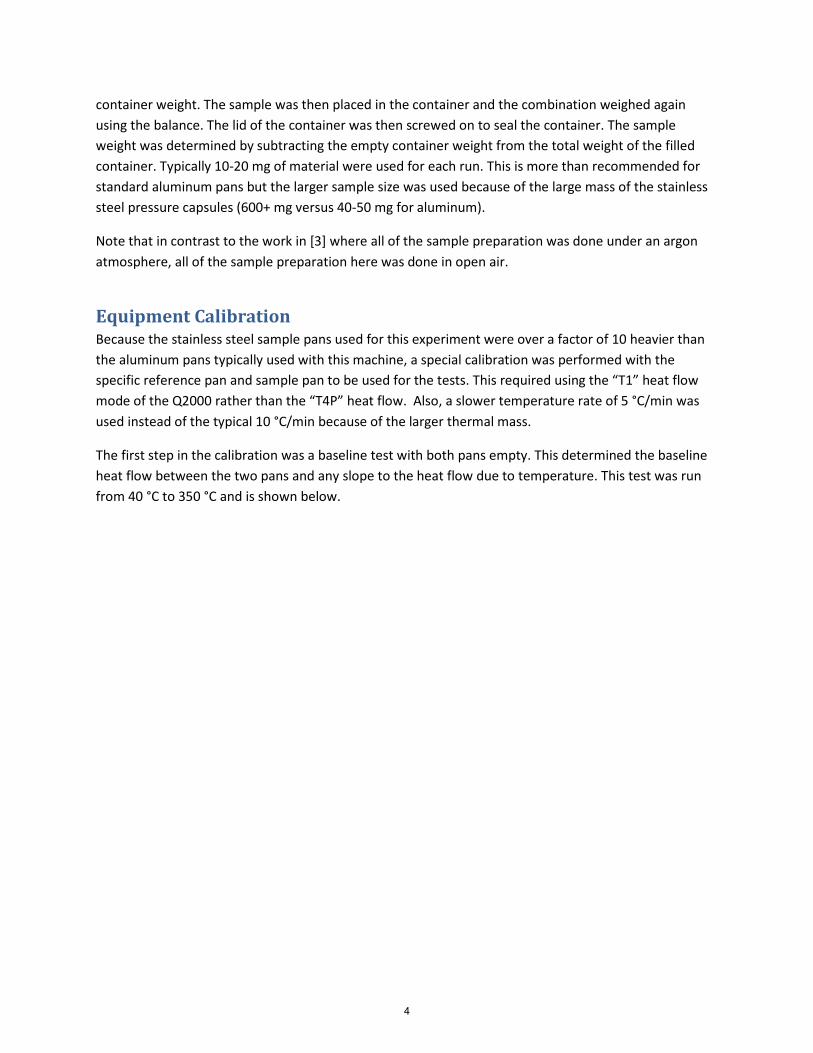
The first step in the calibration was a baseline test with both pans empty. This determined the baseline heat flow between the two pans and any slope to the heat flow due to temperature. This test was run from 40 °C to 350 °C and is shown below.
4
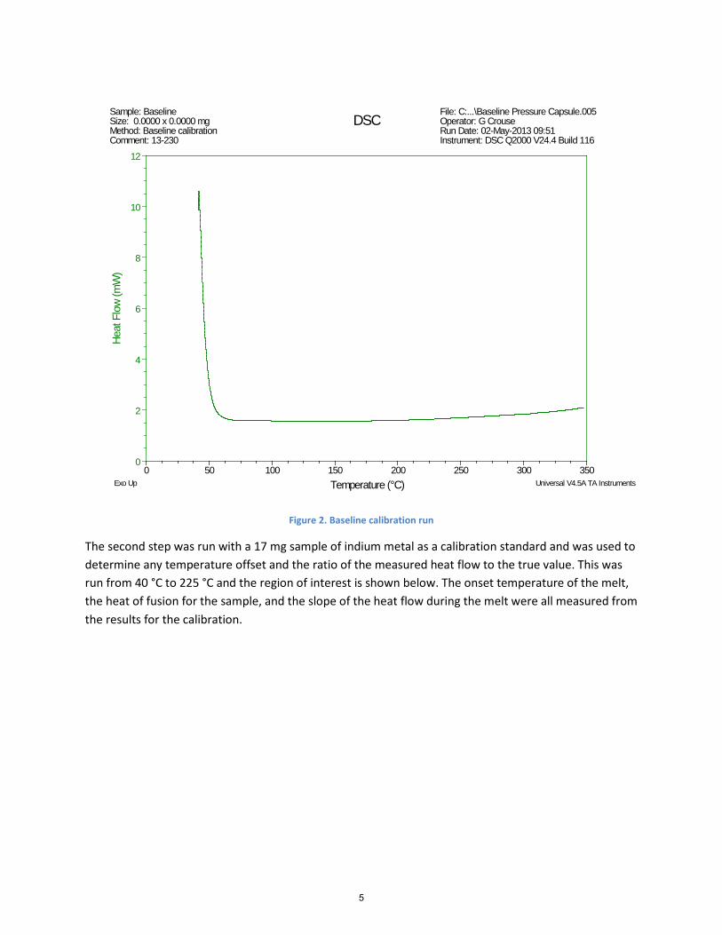
Figure 2. Baseline calibration run
The second step was run with a 17 mg sample of indium metal as a calibration standard and was used to determine any temperature offset and the ratio of the measured heat flow to the true value. This was run from 40 °C to 225 °C and the region of interest is shown below. The onset temperature of the melt, the heat of fusion for the sample, and the slope of the heat flow during the melt were all measured from the results for the calibration.
0
2
4
6
8
10
12
Heat
Flo
w (m
W)
0 50 100 150 200 250 300 350Temperature (°C)
Sample: BaselineSize: 0.0000 x 0.0000 mgMethod: Baseline calibrationComment: 13-230
DSCFile: C:...\Baseline Pressure Capsule.005Operator: G CrouseRun Date: 02-May-2013 09:51Instrument: DSC Q2000 V24.4 Build 116
Exo Up Universal V4.5A TA Instruments
5

Figure 3. Indium calibration run
Based on these two calibration runs, the calibration parameters were determined and input to the system to correct the experimental results. The complete set of calibration parameters are presented in the following table.
Table 1. DSC calibration data, May 02, 2013
T1 Baseline Slope -0.001 µV/°C Offset 5.8632 µV Indium Cell Constant 1.0540 Onset Slope -8.3220 mV/°C Observed Melt Temperature 159.6 °C Correct Melt Temperature 156.6 °C
After the calibration two additional runs were completed, one with empty sample pans and one with the indium calibration standard. The empty pan run was used as a more detailed baseline for adjusting the following runs. The default calibration uses an offset and slope correction to adjust for baseline. It was
161.06°C
159.60°C27.24J/g
-8.322mW/°C
-15
-10
-5
0
5
Heat
Flo
w (m
W)
158.5 159.0 159.5 160.0 160.5 161.0 161.5 162.0 162.5Temperature (°C)
Sample: IndiumSize: 17.1200 x 0.0000 mgMethod: Cell constant calibrationComment: 13-230
DSCFile: Indium Pressure Capsule.002.Calibrati...Operator: G CrouseRun Date: 01-May-2013 15:42Instrument: DSC Q2000 V24.4 Build 116
Exo Up Universal V4.5A TA Instruments
6
observed however that the baseline changed significantly between the heating cycle and the cooling cycle. Using this empty cell run as a baseline allowed the correction of the data runs for these effects. The empty cell run is shown in Figure 4.
Figure 4. Empty cell baseline run
The run with the indium sample is shown below in Figure 5. The onset temperature is measured at 155.98 °C and the heat of fusion is 29.00 J/g. The true values are 156.6 °C and 28.71 J/g respectively for a 0.4% error in temperature and 1.0% error in heat.
-20
0
20
40
60
Heat
Flo
w (m
W)
0 50 100 150 200 250 300Temperature (°C)
Sample: Empty CellSize: 0.0000 mgMethod: Crouse-BLPComment: 13-231
DSCFile: C:...\Run-0502-03-EmptyCell.001Operator: G CrouseRun Date: 02-May-2013 15:16Instrument: DSC Q2000 V24.4 Build 116
Exo Up Universal V4.5A TA Instruments
7

Figure 5. Indium sample data check
Experimental Results The first test runs were of the individual reagents. Figure 6 shows the analysis of Cu(OH)2 from 100 to 240 °C. In that temperature range copper(II) hydroxide decomposes into copper oxide and water vapor. The reaction is endothermic and results indicate 363.1 J/g of heat were required with an onset temperature of 150.32 °C. The measured value corresponds closely to the value of 368.65 J/g measured by Mills [3]. The decomposition reaction is
Cu(OH)2 → CuO + H2O
and the thermochemistry data for the reagents is listed below in Table 2. Based on the heats of fusion in Table 2, the decomposition would theoretically require 86.92 J/g for decomposition to liquid water or 527.5 J/g for decomposition to steam. The experimental result lies between these two values but much closer to the upper number. Since the decomposition occurs well above the boiling point of water but in a sealed container, it would be anticipated that much but not all of the H2O would undergo the phase change to steam and the experimental result is consistent with that assumption.
157.52°C
155.98°C29.00J/g
-1.0
-0.8
-0.6
-0.4
-0.2
0.0
0.2
Heat
Flo
w (W
/g)
150 155 160 165 170 175Temperature (°C)
Sample: Indium CheckSize: 17.0000 mgMethod: Crouse-IndiumComment: 13-230
DSCFile: C:...\Run-0502-01-Indium.001Operator: G CrouseRun Date: 02-May-2013 11:26Instrument: DSC Q2000 V24.4 Build 116
Exo Up Universal V4.5A TA Instruments
8

Table 2. Thermochemistry Data for Cu(OH)2 Decomposition [9]
Compound Molecular Weight Enthalpy of Formation (kJ/mol std conditions)
Cu(OH)2 97.561 -450.37 CuO 79.545 -156.06
H2O 18.0153 -241.83 (gas) -285.83 (liquid)
Figure 6. DSC analysis of Cu(OH)2
Figure 7 shows an analysis of CuBr2 alone. A number of features are seen in the graph, but it is not clear what they represent. At 498 °C, the melting point of CuBr2 is far higher than the range tested and the specification for the material from the supplier indicated very high purity. Moreover, these sorts of features were not noted in the results published by Mills [3]. Over the course of these experiments, several test cells exhibited signs of leakage and the features may be evidence of that leakage or other artifacts.
150.47°C
150.32°C363.1J/g
-3
-2
-1
0
1
Heat
Flo
w (W
/g)
100 120 140 160 180 200 220 240Temperature (°C)
Sample: Cu(OH)2Size: 10.8200 mgMethod: Crouse-BLPComment: 13-232
DSCFile: C:...\Run-0502-04-CuOH2.001Operator: G CrouseRun Date: 02-May-2013 17:21Instrument: DSC Q2000 V24.4 Build 116
Exo Up Universal V4.5A TA Instruments
9
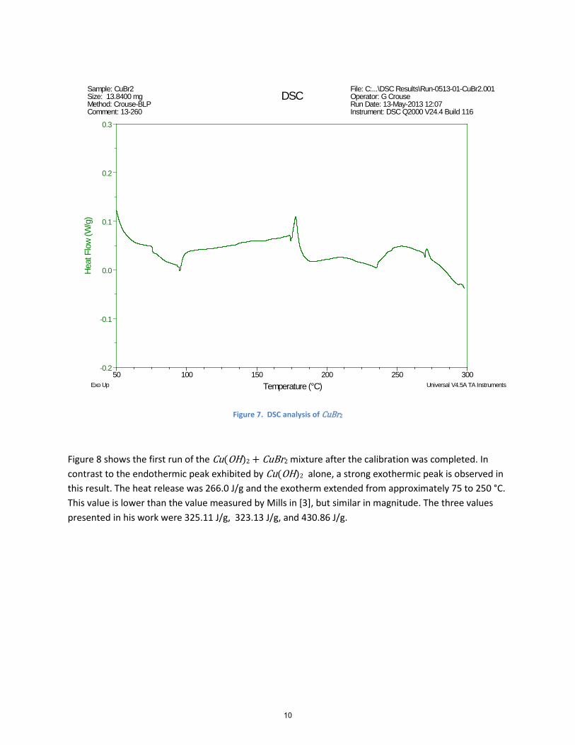
Figure 7. DSC analysis of CuBr2
Figure 8 shows the first run of the Cu(OH)2 + CuBr2 mixture after the calibration was completed. In contrast to the endothermic peak exhibited by Cu(OH)2 alone, a strong exothermic peak is observed in this result. The heat release was 266.0 J/g and the exotherm extended from approximately 75 to 250 °C. This value is lower than the value measured by Mills in [3], but similar in magnitude. The three values presented in his work were 325.11 J/g, 323.13 J/g, and 430.86 J/g.
-0.2
-0.1
0.0
0.1
0.2
0.3
Heat
Flo
w (W
/g)
50 100 150 200 250 300Temperature (°C)
Sample: CuBr2Size: 13.8400 mgMethod: Crouse-BLPComment: 13-260
DSCFile: C:...\DSC Results\Run-0513-01-CuBr2.001Operator: G CrouseRun Date: 13-May-2013 12:07Instrument: DSC Q2000 V24.4 Build 116
Exo Up Universal V4.5A TA Instruments
10
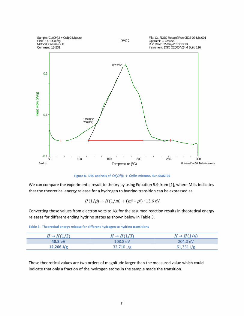
Figure 8. DSC analysis of Cu(OH)2 + CuBr2 mixture, Run 0502-02
We can compare the experimental result to theory by using Equation 5.9 from [1], where Mills indicates that the theoretical energy release for a hydrogen to hydrino transition can be expressed as:
H (1/p) → H (1/m) + (m2 – p2) ∙ 13.6 eV
Converting those values from electron volts to J/g for the assumed reaction results in theoretical energy releases for different ending hydrino states as shown below in Table 3.
Table 3. Theoretical energy release for different hydrogen to hydrino transitions
H → H (1/2) H → H (1/3) H → H (1/4) 40.8 eV 108.8 eV 204.0 eV
12,266 J/g 32,710 J/g 61,331 J/g
These theoretical values are two orders of magnitude larger than the measured value which could indicate that only a fraction of the hydrogen atoms in the sample made the transition.
177.20°C
115.87°C266.0J/g
-0.1
0.1
0.3
Heat
Flo
w (W
/g)
50 100 150 200 250 300Temperature (°C)
Sample: Cu(OH)2 + CuBr2 MixtureSize: 14.1900 mgMethod: Crouse-BLPComment: 13-231
DSCFile: C:...\DSC Results\Run-0502-02-Mix.001Operator: G CrouseRun Date: 02-May-2013 13:18Instrument: DSC Q2000 V24.4 Build 116
Exo Up Universal V4.5A TA Instruments
11
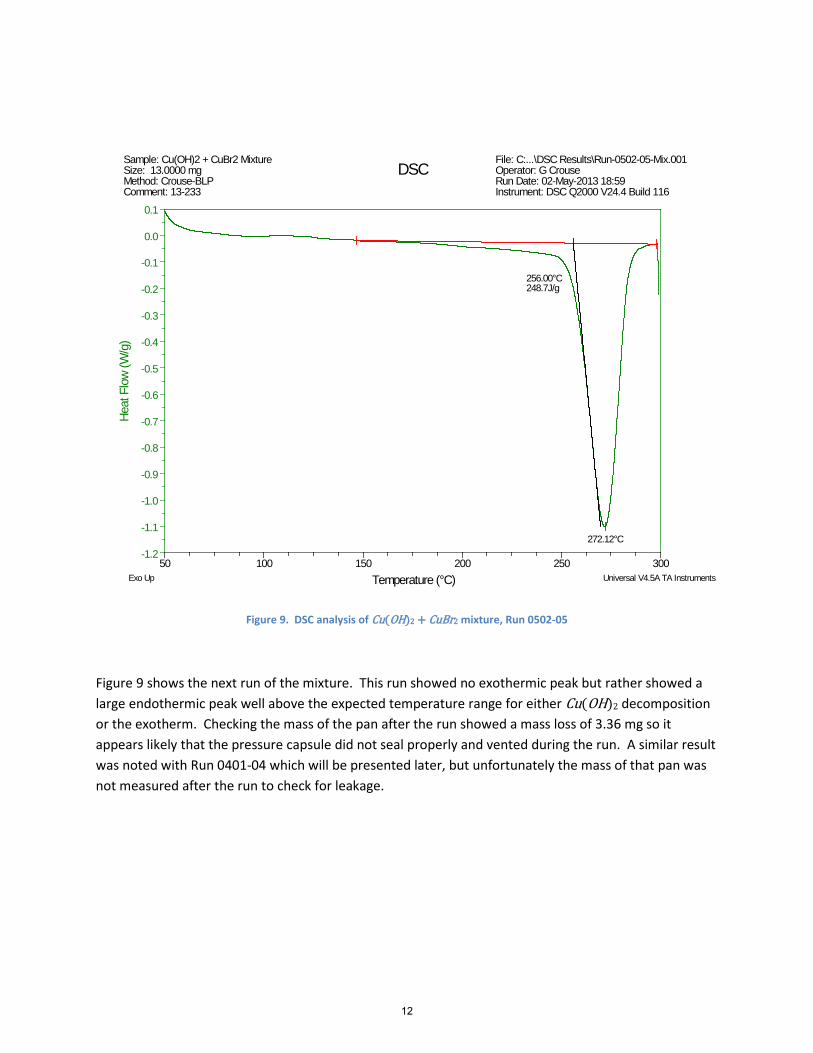
Figure 9. DSC analysis of Cu(OH)2 + CuBr2 mixture, Run 0502-05
Figure 9 shows the next run of the mixture. This run showed no exothermic peak but rather showed a large endothermic peak well above the expected temperature range for either Cu(OH)2 decomposition or the exotherm. Checking the mass of the pan after the run showed a mass loss of 3.36 mg so it appears likely that the pressure capsule did not seal properly and vented during the run. A similar result was noted with Run 0401-04 which will be presented later, but unfortunately the mass of that pan was not measured after the run to check for leakage.
272.12°C
256.00°C248.7J/g
-1.2
-1.1
-1.0
-0.9
-0.8
-0.7
-0.6
-0.5
-0.4
-0.3
-0.2
-0.1
0.0
0.1
Heat
Flo
w (W
/g)
50 100 150 200 250 300Temperature (°C)
Sample: Cu(OH)2 + CuBr2 MixtureSize: 13.0000 mgMethod: Crouse-BLPComment: 13-233
DSCFile: C:...\DSC Results\Run-0502-05-Mix.001Operator: G CrouseRun Date: 02-May-2013 18:59Instrument: DSC Q2000 V24.4 Build 116
Exo Up Universal V4.5A TA Instruments
12

Figure 10. DSC analysis of Cu(OH)2 + CuBr2 mixture, Run 0513-02
Figure 10 and Figure 11 show two additional tests of the Cu(OH)2/CuBr2 mixture. Both show the exothermic peak. The two runs showed similar onset temperatures, heat release, and peak temperatures. Figure 12 plots all five of the mixture runs that exhibited exothermic peaks together on one graph for comparison. The first two runs shown in the figure were completed before the machine was recalibrated for the pressure capsules. Hence the heat measurements are somewhat suspect. The bottom three runs were completed after the calibration. These three show very similar characteristics. Compared to the results from [3], the peaks are somewhat smaller and the onset is much more gradual. These differences may be partially explained by the slower heating rate (5 °C/min vs 10 °C/min) and the sample preparation may also have affected the results. These samples were prepared in air versus and argon atmosphere in [3].
Figure 13 compares the two runs that exhibited endothermic peaks. In both the peak occurs at a much higher temperature than the decomposition peak exhibited by Cu(OH)2 alone (Figure 6) and above the temperature where the exothermic peak was expected. In both cases, it appears that the pressure
192.86°C
125.28°C296.0J/g
-0.1
0.0
0.1
0.2
0.3
0.4
Heat
Flo
w (W
/g)
50 100 150 200 250 300Temperature (°C)
Sample: Cu(OH)2 + CuBr2 MixtureSize: 14.3800 mgMethod: Crouse-BLPComment: 13-261
DSCFile: C:...\DSC Results\Run-0513-02-Mix.001Operator: G CrouseRun Date: 13-May-2013 14:48Instrument: DSC Q2000 V24.4 Build 116
Exo Up Universal V4.5A TA Instruments
13

capsule leaked during the run and this loss of pressure in the capsule prevented the reaction from occurring.
The results from the various DSC runs are summarized in Table 4 below and includes onset temperatures, integrated heat for any peaks seen in the data, and temperature for peak heat flow for any peaks. The recalibration is noted in the table to indicate which runs were completed before and which were completed after the recalibration was done.
Figure 11. DSC analysis of Cu(OH)2 + CuBr2 mixture, Run 0513-04
196.84°C
114.85°C334.1J/g
-0.2
-0.1
0.0
0.1
0.2
0.3
Heat
Flo
w (W
/g)
50 100 150 200 250 300Temperature (°C)
Sample: Cu(OH)2 + CuBr2 MixtureSize: 14.7400 mgMethod: Crouse-BLPComment: 13-263
DSCFile: C:...\DSC Results\Run-0513-04-Mix.001Operator: G CrouseRun Date: 13-May-2013 19:01Instrument: DSC Q2000 V24.4 Build 116
Exo Up Universal V4.5A TA Instruments
14
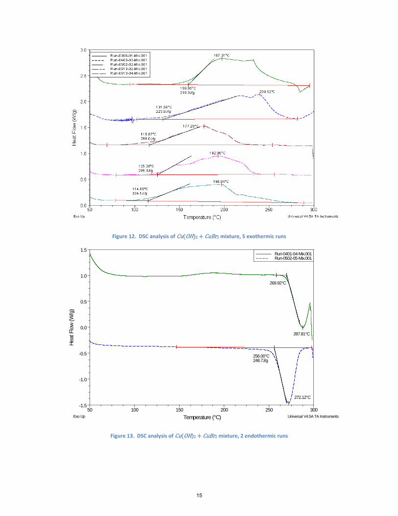
Figure 12. DSC analysis of Cu(OH)2 + CuBr2 mixture, 5 exothermic runs
Figure 13. DSC analysis of Cu(OH)2 + CuBr2 mixture, 2 endothermic runs
287.81°C
269.92°C
272.12°C
256.00°C248.7J/g
-1.5
-1.0
-0.5
0.0
0.5
1.0
1.5
Heat
Flo
w (W
/g)
50 100 150 200 250 300Temperature (°C)
Run-0401-04-Mix.001––––––– Run-0502-05-Mix.001– – – –
Exo Up Universal V4.5A TA Instruments
15
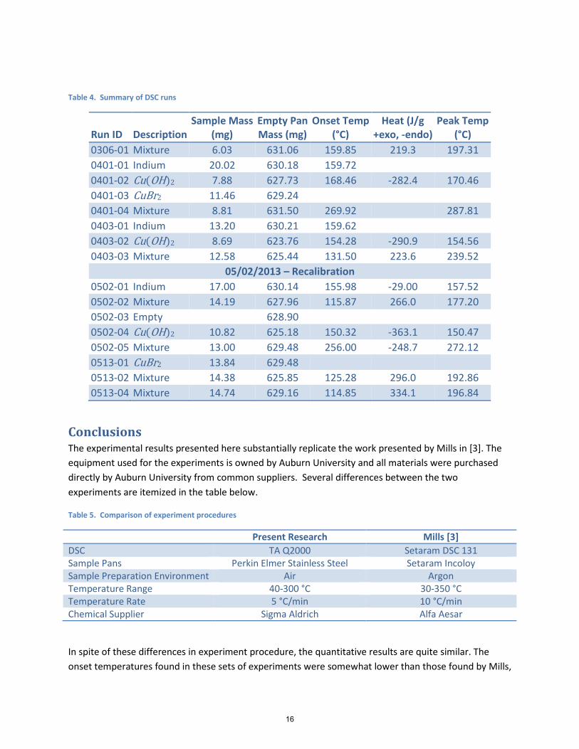
Table 4. Summary of DSC runs
Run ID Description Sample Mass
(mg) Empty Pan Mass (mg)
Onset Temp (°C)
Heat (J/g +exo, -endo)
Peak Temp (°C)
0306-01 Mixture 6.03 631.06 159.85 219.3 197.31 0401-01 Indium 20.02 630.18 159.72 0401-02 Cu(OH)2 7.88 627.73 168.46 -282.4 170.46 0401-03 CuBr2 11.46 629.24 0401-04 Mixture 8.81 631.50 269.92 287.81 0403-01 Indium 13.20 630.21 159.62 0403-02 Cu(OH)2 8.69 623.76 154.28 -290.9 154.56 0403-03 Mixture 12.58 625.44 131.50 223.6 239.52
05/02/2013 – Recalibration 0502-01 Indium 17.00 630.14 155.98 -29.00 157.52 0502-02 Mixture 14.19 627.96 115.87 266.0 177.20 0502-03 Empty 628.90 0502-04 Cu(OH)2 10.82 625.18 150.32 -363.1 150.47 0502-05 Mixture 13.00 629.48 256.00 -248.7 272.12 0513-01 CuBr2 13.84 629.48 0513-02 Mixture 14.38 625.85 125.28 296.0 192.86 0513-04 Mixture 14.74 629.16 114.85 334.1 196.84
Conclusions The experimental results presented here substantially replicate the work presented by Mills in [3]. The equipment used for the experiments is owned by Auburn University and all materials were purchased directly by Auburn University from common suppliers. Several differences between the two experiments are itemized in the table below.
Table 5. Comparison of experiment procedures
Present Research Mills [3] DSC TA Q2000 Setaram DSC 131 Sample Pans Perkin Elmer Stainless Steel Setaram Incoloy Sample Preparation Environment Air Argon Temperature Range 40-300 °C 30-350 °C Temperature Rate 5 °C/min 10 °C/min Chemical Supplier Sigma Aldrich Alfa Aesar
In spite of these differences in experiment procedure, the quantitative results are quite similar. The onset temperatures found in these sets of experiments were somewhat lower than those found by Mills,
16
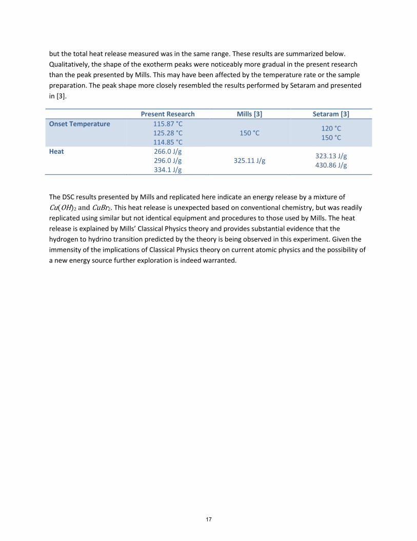
but the total heat release measured was in the same range. These results are summarized below. Qualitatively, the shape of the exotherm peaks were noticeably more gradual in the present research than the peak presented by Mills. This may have been affected by the temperature rate or the sample preparation. The peak shape more closely resembled the results performed by Setaram and presented in [3].
Present Research Mills [3] Setaram [3] Onset Temperature 115.87 °C
125.28 °C 114.85 °C
150 °C 120 °C 150 °C
Heat 266.0 J/g 296.0 J/g 334.1 J/g
325.11 J/g 323.13 J/g 430.86 J/g
The DSC results presented by Mills and replicated here indicate an energy release by a mixture of Cu(OH)2 and CuBr2. This heat release is unexpected based on conventional chemistry, but was readily replicated using similar but not identical equipment and procedures to those used by Mills. The heat release is explained by Mills’ Classical Physics theory and provides substantial evidence that the hydrogen to hydrino transition predicted by the theory is being observed in this experiment. Given the immensity of the implications of Classical Physics theory on current atomic physics and the possibility of a new energy source further exploration is indeed warranted.
17

References
[1] R. L. Mills, The Grand Unified Theory of Classical Physics, Cranbury, NJ: BlackLight Power Inc., 2011.
[2] H. A. Haus, "On the radiation from point charges," American Journal of Physics, vol. 54, pp. 1126-1129, 1986.
[3] R. L. Mills, J. Lotoski, W. Good and J. He. [Online]. Available: http://www.blacklightpower.com/wp-content/uploads/papers/DSCsolidfuels.pdf. [Accessed 09 05 2013].
[4] TA Instruments, [Online]. Available: http://www.tainstruments.com/product.aspx?id=15&n=1&siteid=11. [Accessed 09 05 2013].
[5] PerkinElmer, "Stainless Steel High Pressure Capsules," [Online]. Available: http://www.perkinelmer.com/Catalog/Product/ID/B0182901. [Accessed 09 05 2013].
[6] Thermal Support, Inc., [Online]. Available: http://www.thermalsupport.com/product.php?id=187&category=1&search=. [Accessed 09 05 2013].
[7] Sigma-Aldrich, [Online]. Available: http://www.sigmaaldrich.com/catalog/product/aldrich/289787?lang=en®ion=US. [Accessed 09 05 2013].
[8] Sigma-aldrich, [Online]. Available: http://www.sigmaaldrich.com/catalog/product/aldrich/437867?lang=en®ion=US. [Accessed 09 05 2013].
[9] M. W. Chase Jr., "NIST-JANAF Themochemical Tables, 4th Edition," J. Phys. Chem. Ref. Data, Monograph 9, pp. 1-1951, 1998.
18