diffusion ii barker wednesday...
TRANSCRIPT
DIFFUSION IN HYDROGELOGY
John Barker (University of Southampton)
Funding:
DIFFUSION FUNDAMENTALS II
AUG 2007

OUTLINE
WHAT IS HYDROGEOLOGY?OCCURRENCE OF THE DIFFUSION EQUATIONCHALLENGES IN HYDROGEOLOGY
PUMPING TESTSUSE OF TRACERSMEASUREMENTS OF DIFFUSION
MODELLING: DOUBLE POROSITY & LAPLACE TRANSFORMS
KEY POINTSPLEASE ‘LET ME KNOW…’

HYDROGEOLOGY
Water resources: quantity and qualityGeotechnics (mining, dams, dewatering, slope stability,…)FloodingEnvironmental preservation (e.g. streams, wetlands) Decontamination (e.g. soils and water)Waste disposal (e.g. radwaste and landfill)Geothermal energy Oil and gas extractionCO2 sequestration
ONE DEFINITION: Hydrogeology is the study of groundwater (water below the ground surface) and its qualities: flow, amount, speed, direction, sustainability, extraction or replenishment capabilities.

Fetter, 1994
Water volumes: world
98% of liquid fresh water is Groundwater

Hydrologic Cycle
Fetter, 1994GROUNDWATER

Hazards to water quality

Diffusion Equations
Heat: Fourier’s law
Solute (e.g. pollutants): Fick’s laws
Flow: Darcy’s law

BRIEF MENTION OF ‘HEAT’
Summer: hot water can be stored for winter heating. Winter: cool water can be stored for summer cooling.

MOLECULAR DIFFUSION: Long times
Observed diffusion profile for helium in a clay formation with a fitted diffusion (with production) model. A D value of about 3×10-11
m2/s over a distance of about 250 m gives a characteristic time of 10 to 50 Ma.
Mont Terri underground rock laboratory in Switzerland

Henry Darcy, 1856. Détermination des loisd'écoulement de l'eau àtravers le sable. Les Fontaines Publiques de la Ville de Dijon, Paris, Victor Dalmont, pp.590 - 594
DARCYS LAW: Darcy’s Experiment
Darcy’s Law:
Flow rate=K×Area ×Head Gradient
K=‘hydraulic conductivity’Or ‘permeability’

Why do rivers flow when it is dry?
( )hDth
H∇∇=∂∂ .
L
h
h is head = water level in wells
Hydraulic Diffusivity

Why do rivers flow when it is dry?
HDLt 2
ydiffusivit hydraulicdistanceconstant time
2
≈=t
= Major rainfall event

NATURAL FLUCTUATIONS: Verification of ‘Fick’s Second Law’
Fluctuations of the Elbe River (near the sea) and water table levels in wells at various distances from the river (after Werner and Norden)
Wells
River

Solution of the diffusion equation:
( )02( , ) exp sinMSL shift
H
h x t H H x t tTD Tπ π⎛ ⎞ ⎛ ⎞= + − −⎜ ⎟ ⎜ ⎟⎜ ⎟ ⎝ ⎠⎝ ⎠
i.e. exponentially decaying with time (phase) shift of
4shiftH
Tt xDπ
=
Both the amplitude and time shift depend are determined by the ‘hydraulic diffusivity’, DH.
Validates Hydraulic “Fick’s Second Law”)

CHALLENGES
HETEROGENEITY
INACCESSIBILITY

HETEROGENEITY

HETEROGENEITY
Fractrure apertures range over several
orders of magnitude and flow rate is proportional
to the cube of the aperture.

Heterogeneity: Anthropogenic

HETEROGENEITY: Microscopic

HETEROGENEITY: Self-Organisation
HETEROGENEITY CHANNEL FLOW ‘DEAD’ ZONES

HETEROGENEITY: Flow dimension?
FORCED FLOW TO CENTRAL POINT
Heterogeneous 2D system Flow dimension < 2D
Porosity Major flow paths
Barker (1988) “Flow dimension should be treated as an empirical value which may be non-integer”
Similar to experiment described by Charles
Nicholson:‘probe molecules’ to brain.

Flow Dimensions: a problem
Following 1988 paper many measurements in fractured rock indicate flow to a well typically has a dimension of 1.4 to 1.7.
But how do we use that value in a regional groundwater model? That is, how do we get H(x,y,z,t) rather than H(r,t).
Perhaps flow on a fractal.

Random walk on a fractal: work by Shaun Sellers
19,683×19,683 lattice
For each fixed origin, we created an ensemble of walkers (typically 30,000-50,000 particles) with total time steps ranging from 1 million to 100 million.
Power law depends on time and start point and direction.
SO
None of the proposed equations such as that below work well.
⎟⎠⎞
⎜⎝⎛
∂∂
∂∂
=∂∂ +−
− ),(),( 11
0 trHr
rrr
DtrHt
wf
f
ddd

DATA?
INACCESSIBILITYof subsurface

INACCESSIBILITY:Radwaste
Target depth of repository typically 300 to 2000 metres below
ground level

PUMPING TESTS:Radial flow to a pumped well
Probably the most important field technique in hydrogeology.
Determines the permeability and diffusivity.
Heterogeneity? Radial diffusion averages properties. HOW EXACTLY? – IS THIS KNOWN IN OTHER FIELDS?

A major tool: the pumping test
We measure the drop in water table as a function of time:
s(r,t)
Water table during pumping
Initial water table
∂ ∂ ∂⎛ ⎞= ⎜ ⎟∂ ∂ ∂⎝ ⎠HDs sr
t r r r

A large-diameter ‘dug’ well

Deepening a large-diameter well

A rectangular ‘well’

TRACER TESTS
USED TO DETERMINE:
Flow paths (connection)
Velocities (arrival times, protection)
Flow and transport properties

Tracers in HydrogeologyParticles: e.g. Lycopodium spores, Microspheres
Microbiological: e.g. Phage, Bacterial spores
Inorganic salts: e.g. Cl, Li
Fluorescent dyes: e.g. Rhodamine WT, RhodamineB, Fluorescein
Fluorocarbons: e.g. SF6, freon (CFC-12)
Isotopes: e.g. Br-82, Cl-36, I, Tritiated water, Deuterated water

Historical Tracers
~330 BC Alexander the Great: Sinking River Rhigadanus:TRACER=Two Dead Horses
~10 AD Tetrach Philippus: Source of the Jordan: TRACER=Chaff
1901 Pernod Factory at Pontarlier: River Doube: TRACER=Absinthe (Accident)

TRACERS IN HYDROGEOLOGY Will I ever see any of this
againanywhere?

0.1
1
10
100
28/01/05 04/02/05 11/02/05 18/02/05
Log
Flu
ores
cein
(μ
g/l)
Injection 1 Injection 2
Results of tracer test over 4 km.
Velocity ≈ 5 km/day
Success – This time
Long tail is charcteristic of ‘double-porosity’ behaviour (later)
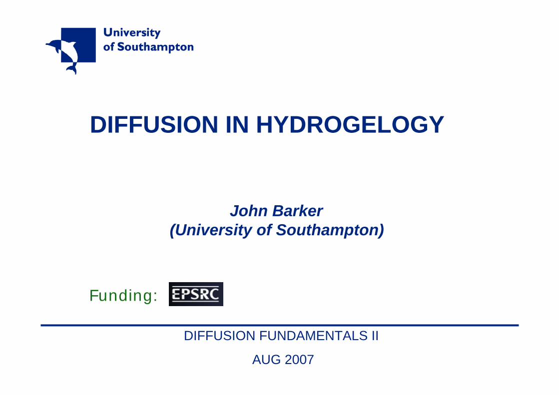
Laboratory: Closed system

University of Southampton Waste Research Cell. Diameter = 2m.
Waste is compressed to represent a particular depth in a landfill.
CURRENT TEST AT PITSEA
Currently performing a tracer test

Dilution of the Pitsea brew…
30 days

Results so far…
0.000
0.100
0.200
0.300
0.400
0.500
0.600
0.700
0.800
0.900
1.000
1.100
0.0 5.0 10.0 15.0 20.0 25.0 30.0
Time (days)
Con
cent
ratio
n in
Mob
ile (F
ract
ure)
Por
osity
EC data
BromidedataModelledBromideModelledLithiumModelledD2O
tcb=50 dayssigma=10
Awaiting lab analysis validation?

SOME DIFFUSION MEASURMENTS

Rapid measurement of D

Measuring D for Cl in a 1-inch chalk plug
Electric Stirrer
Reference Electrode
Water
To PC
Ion-Selective Electrode
Air (Atmospheric Pressure)
From Water Bath
To Water Bath
To PC
Rotating Chalk Plug
0 2c2 cm

Help! – an anomaly
Diffusion Cell Data (PCE and Cl)
0.7
0.8
0.9
1.0
1 100 10000
Time (min)
Rel
ativ
e C
once
ntra
tion
Cl - Data
Cl-Fit
PCE-Data
PCE-Fit
Diffusion cell data.Annular concentrations show a lag of chloride behind PCE (anomalously) indicating that the latter is diffusing faster. The asymptotic values give the same porosity, in agreement with the known value, indicating negligible retardation.
PCE:-UPAC name: trichloroetheneMolecular formula: C2HCl3Molar mass: 131.39 g mol-1
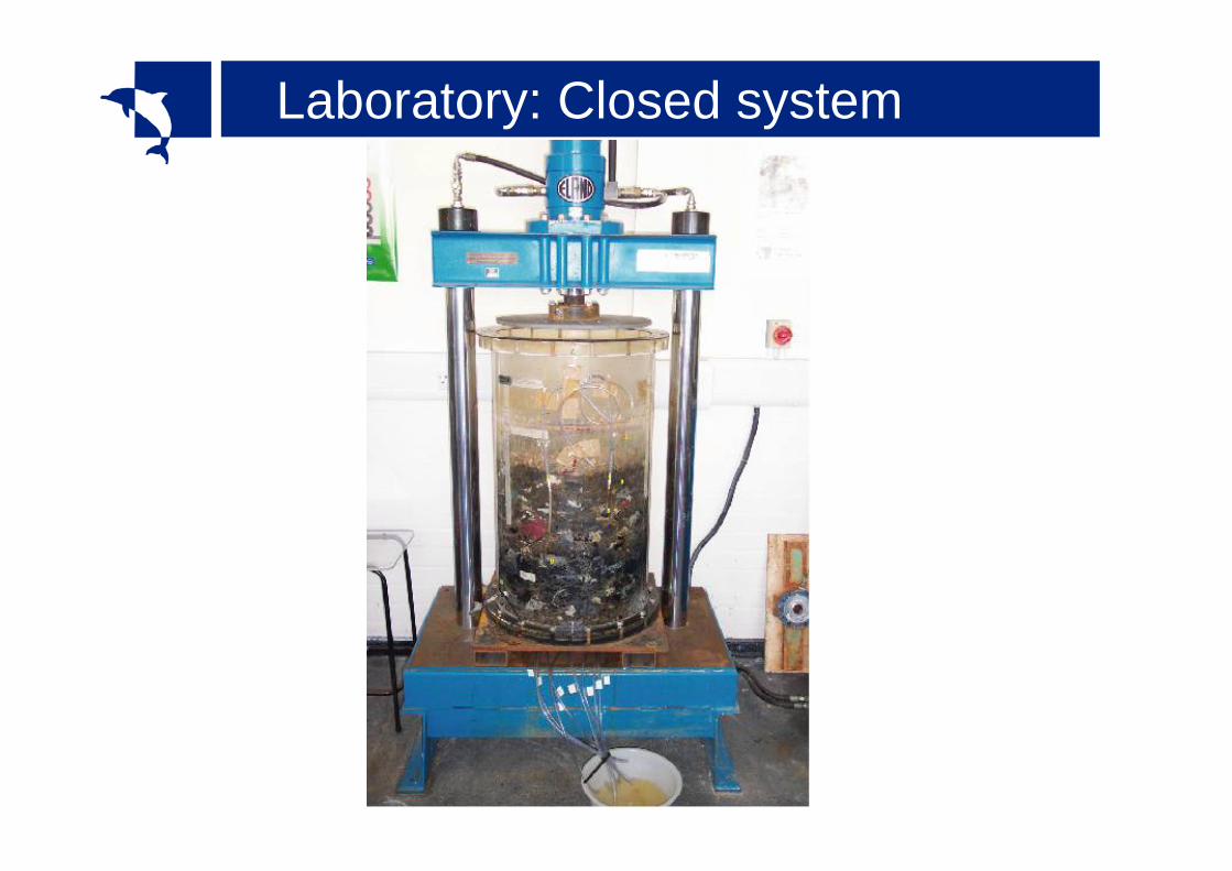
Tomographic X-ray fluorescence (TXRF)
Perspex holder with tube mounted through its base
Resin coating outer suface of sample
Direction of circulating tracer solution.
Line of points at progressively greater distance from the exposed surface at which spectra are recorded.
15 mm
10 mm Sample placed in section cut into tubing so a single face is exposed to the tracing solut ion.
Tracer ions can diffuse freely across exposed face of saturated sample.
Front section
Side section
Incident synchrotron
beam
Resin seal
Fluorescent emissions
Sample
Circulating tracer fluid Perspex
base
M. Betson, Barker, J.A., Barnes, P. & Atkinson, T.C. (2005) Use of Synchrotron Tomographic Techniquesin the Assessment of Diffusion Parameters for Solute Transport in Groundwater Flow. Transport In Porous Media, 60(2): 217–223.
Chalk sample
Diffusion from circulating water
X-ray measurements
Method was introduced on Tuesday by
Gero Vogel

Results
Relative concentrations versus time. (Vertical line.)
C obtained from tracer-ion X-ray fluorescence intensities
Sample: ChalkScan Height: 9mm
Model: Cl
MODELLING
MAINLY:-DOUBLE-POROSITY
TWO FUNCTIONS CHARACTERIZING GEOMETRY
LAPLACE TRANSFORM SOLUTIONS

A ‘Double-Porosity’ Medium
DP Model: flow in ‘fractures’ diffusion into ‘matrix’
Usually: Fractures and matrix co-exist: 6-D model.

Transport through a channel in a porous medium filled with porous blocks
Advection in channel
Blocks
Diffusive exchange with immobile pore water
Similar figure on poster
B10
(Denis Grebenkov)
Formulations probably
interchangeable

Transport through channel – contd.
( ) ( )[ ] cccba
pt
ptptptpc
dttxcepxc
CB1exp),0(
),(),(0
ρσ ++−=
= ∫∞
−
c(x,t)
t
c(0,t)
Laplace transform solution for output concentration:
t
Focus on the B() and C() functions

[ ]π
μ=
+1( , )
C( )wc
T s r tQ p t p
Similarly: LT solution for pumping from a well in a double-porosity rock.
μ σ⎡ ⎤= +⎣ ⎦2 1 B( )w at p t p
C() represents the well shape, normally a
circle.where
B() represents the ‘block shape’
Here the diffusion is ‘hydraulic’: both in the fractures and the rock matrix blocks.

( ) 2 ii
Bn
β ψζ ψζ Ω
Γ
∂= =
∂2 2 2 in
1 oni
i
β ψ ζ ψψ∇ = Ω
= Γ
α ψζζ Γ
∂=
∂2( )e
Cn
2 2 2 in1 on
e
e
α ψ ζ ψψ
∇ = Ω
= Γ
n
iΩ
iΓ
eΩ
eΓ
n
Definitions of B(x) and C(x)
In the time domain obtain solution as sum of exponentials.
Familiar? Probably discovered in may fields?

Typical block geometries
SLABS SPHERES MIXTURES

An atypical ‘block geometry’
Development of mathematical model for cooling the fish with iceJournal of Food Engineering 71 (2005) 324–329
Charles NicholsonSuggested a variety of novel
geometries.

Also known as ‘shape factors’ and ‘effectiveness factors’ (by chemical engineers).OTHER NAMES?
GEOMETRY BGF, B(x) Characteristic length, b
Slab (tanh x)/x Half slab thickness
Cylinder (infinite) I1(2x)/x I0(2x) Half radius
Sphere (coth 3x)/x – 1/3x2 One-third of radius
n-D Sphere In/2(nx)/x In/2-1(nx) Radius / n
Some Block-Geometry Functions
b=Bock volume/Block area
First-order exchange ∝ k(cf-cm), B(x)=k/(k+x2) BEST k or k’s?
Appears inB26
(Traytak & Traytak)which uses spherical
geometry.Could be generalized
to B()

0
0.2
0.4
0.6
0.8
1
1.2
-2.00 -1.50 -1.00 -0.50 0.00 0.50 1.00 1.50 2.00log ζ
B(
)
infinite slabinfinite cylinderspherecubeinfinite hollow cylinder
Block Geometry Functions, B(x)
Similar when ‘distance scale’ = volume/contact area.

B(x) for ‘spheres’ of various dimensions
BGF for n-Sphere
0
0.1
0.2
0.3
0.4
0.5
0.6
0.7
0.8
0.9
1
0.1 1 10 100
x
B(x,
n)
0.01
0.02
0.05
0.1
0.2
0.5
1
2
5
∞
2
12/
2/
4112),B(
)2()2(),B(
xx
xxIxInx
n
n
++=∞
=− What does a sphere of
dimension ½ look like?
1D: Slab
2D: Cylinder
3D: Sphere
n
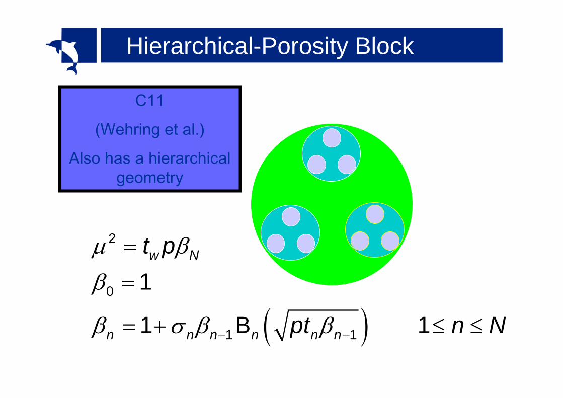
Hierarchical-Porosity Block
( )
μ ββ
β σ β β− −
=
=
= + ≤ ≤
2
0
1 1
1
1 B 1
w N
n n n n n n
t p
pt n N
C11
(Wehring et al.)
Also has a hierarchical geometry

where
and pi(β) dβ is the proportion by volume of blocks of shape i (i=1,...,Ns) in the size (volume to area) range β to β+ dβ.
ββ β∞
=
⎛ ⎞= ⎜ ⎟⎝ ⎠
∑∫1 0
( ) ( )sN
i ii
xB x p B db
1 0
1 ( )sNi
i
p db
β ββ
∞
=
= ∑∫
Mixtures of Blocks: Candidate for empirical B() functions
Motivation: Extreme heterogeneity especially in waste.

BGF’s for Mixtures of Blocks
BGFs for mixture of two blocks of equal bulk volume for various volume/area ratios = R
Slabs
0
0.20.4
0.6
0.81
1.2
0.0001 0.001 0.01 0.1 1 10 100
x
B(x
) 1101001000
R

Examples of the ‘C’ function
( ) ( ) ( ) ( )( )
( )
ζ ζζ ζ ζ ζ
ξπζζ ξ
ξ ξ
ζ
==
′ −⎡ ⎤= − ⎣ ⎦ −
= = −
⎛ ⎞= ⎜ ⎟⎜ ⎟⎝ ⎠
∑
1 0
22 2 002
2 0
20 0
2
Sheet: C( ) 1/ Circle: C( ) 2 K ( ) /K ( )
,4Ellipse: ,
where cosh 1 , sinh 1 ,
and 8
n n
n n
Fek qC A q
Fek q
e e e
eqE e
These are the ONLY analytical results I have. OTHERS?

Examples of C(): the Channel Geometry Function
-1
0
1
2
3
4
5
6
-3 -2.5 -2 -1.5 -1 -0.5 0 0.5 1log ζ
log
C(
)
circlee=0.4e=0.8e=0.99sheet
e= eccentricity of elliptical channels
NBEllipse tends to
‘slot’ not to sheet

Laplace Transform SolutionsLaplace Transform Solutions
Reminder of the Laplace transform
In praise of LT solutions
Numerical inversion

The Laplace Transform (LT)The Laplace Transform (LT)
0
( ) ( )ptf p e f t dt∞
−= ∫
exp(-a √p)erfc(a/√4t)
1/(p-k)exp(-kt)
1δ(t)
1/p2t
1/p1
( )f p( )f t
∂⇔ −
∂
∂= ∇ ⇔ − = ∇
∂2 2
( ) ( ) (0)
(0)
f t pf s ft
soc D c pc c D ct
Examples
Key operational property
Basis of ‘hybrid’ LT-FD and LT-FE methods.

In praise of LT solutionsIn praise of LT solutions
Simple to obtain and relatively simple compared with time-dependent solutions, which are often not obtainable.
Asymptotic behaviour readily derived
Convolutions simplified
Easy to obtain integrals (e.g. for mass balance)
Moments readily obtained
Numerical inversion is not difficult and allows accurate evaluation at short and long times. (No propagation of errors.)
0( ) ( ) ( ) ( )
tf g t d f p g pτ τ τ− ⇔∫
0( ) ( ) /
tf d f p pτ τ ⇔∫
00
( ) ( ) lim ( 1)N
N N NNp
fE t t f t dtp
∞
→
⎡ ⎤∂= = −⎢ ⎥∂⎣ ⎦∫

Numerical inversion of Laplace Transform: 3 methods
Numerical inversion of exp(0.25/p)/p <=> Jo(sqrt(t))
t=1, Jo(1)=0.765...
0
24
6
8
1012
14
16
0 10 20 30 40
Number of function evaluations
Num
ber o
f sig
nific
ant
figur
es TalbotdeHoogStehfest
( ) ppt ep
dttJe 41
00
1=∫
∞−
Discrete form of the inverse Laplace transform used by Asmund Ukkenberg
and his colleagues in two ‘unnumbered’ posters.

Quick and easy LT inversion
Function Stehfest16(tau As Double) As Double' Stehfest Algorithm coded by JAB for N=16 (Vs is exact)Dim i As Integer, rt As Double, Vs As Variant, Sum As Double, p As DoubleVs = Array(-1 / 2520#, 5377 / 2520#, -33061 / 60#, 6030029 / 180#, -7313986 / 9#, 302285513 / 30#, -3295862234# / 45#, 106803784103# / 315, -147355535079# / 140, 27108159943# / 12, -101991059533# / 30, 35824504617# / 10, -77744822441# / 30, 36811494863# / 30, -2399141888# / 7, 299892736# / 7)rt = 0.693147137704615 / tauSum = 0#For i = 1 To 16
p = i * rtSum = Sum + Vs(i - 1) * Exp(-0.25 / p) / p
Next iStehfest16 = rt * SumEnd Function
The ‘Stehfest’ algorithm coded for 16 function evaluations in VBA (within Excel)
( ) ppt ep
dttJe 41
00
1=∫
∞−

KEY POINTS
HYDROGEOLOGY – WIDE VARIETY OF DIFFUSION PROBLEMS. (I HAD TO LEAVE OUT A LOT!)GEOLOGICAL TIMES ARE LONG (E.G. RADWASTE)CHALLENGES: HETEROGENEITY AND INACCESSIBILITYIMPORTANT TOOLS: PUMPING TESTS & TRACER TESTSCHARACTERIZATION OF DIFFUSION TO BLOCKS AND CHANNELS BY B() AND C().THE LAPLACE TRANSFORM AND ITS NUMERICAL INVERSION

PLEASE LET ME KNOW ABOUT RELATED WORK, ESPECIALLY…
How to use non-integer radial-flow dimension in a 3D (x,y,z) model.
Averaging by radial diffusion in heterogeneous media.
‘Blocks’ in the shape of spheres of non-integer dimension. Meaningful?
Empirical B() functions (c.f. effectiveness factors). And from empirical B() to geometry?
Is the C() function for channels used elsewhere? Analytical results (e.g. slot)?
Hybrid LT-FD or LT-FE methods. (Early papers?)
Asymptotic methods? (Important in waste flushing.)
Could PCE diffuse faster than chloride?

END
Thank you for your attention.
My sincere thanks to the organisers for their invitation.