digital art of bas-relief sculpting - max-planck-institut f¼r informatik

Max-Planck-Institut fur InformatikComputer Graphics GroupSaarbrucken, Germany

Digital Art of Bas-Relief Sculpting

Master Thesis in Computer Science

Computer Science DepartmentUniversity of Saarland

Jens Kerber

Supervisor: Prof. Dr. Hans-Peter Seidel (1st reviewer)Advisor: Prof. Dr. Alexander Belyaev (2nd reviewer)

Max-Planck-Institut fur InformatikComputer Graphics GroupSaarbrucken, Germany

Statement

Hereby I confirm that this thesis is my own work and that I have documentedall sources used.

Saarbrucken, July 31, 2007

Jens Kerber

Declaration of Consent

Herewith I agree that my thesis will be made available through the library ofthe Computer Science Department.

Saarbrucken, July 31, 2007

Jens Kerber

Abstract

In this thesis, we present a semi-automatic method for the generation of bas-reliefs

from a given shape. A Bas-reliefs is an artistic sculptural representation of a three

dimensional scene which possesses a negligible depth.

The main idea behind our method is to work with a range image, whose depth

interval size is compressed in a feature preserving way. Our approach operates in

the gradient domain, whereas we also present an extension which works on the

Laplacian. The algorithm relies on the achievements of High-Dynamic-Range-

Compression and adapts necessary elements to our purpose.

We manipulate the partial derivatives of the range image rather than the image

data itself. These derivatives are compressed by applying an attenuation function

which leads to a relative convergence of the entries. By a feature enhancing tech-

nique we boost small details in order to keep them perceivable in the result. In the

end, the compressed and enhanced partial derivatives are recombined to the final

bas-relief.

The results exhibit a very small depth range but still contain perceptually im-

portant details. A user can specify the desired compression ratio and steer the

relevance of small features in the outcome. The approach is intuitive, fast and

works very well for high compression ratios as experiments have shown.

Possible applications are of artistic nature like sculpting, embossment, engrav-

ing or carving.

i

ii ABSTRACT

Acknowledgement

First, I would like to thank Alexander Belyaev for assigning this interesting project

to me and for his great supervision.

Special thanks to Hans-Peter Seidel for providing an excellent working envi-

ronment in his research group.

I am also grateful to the members of the computer graphics department at the

MPII who were at the right place to the right time and gave me helpful suggestions

when I got stuck; especially Zhao Dong, Dorotea Dudas, Wenhao Song, Carsten

Stoll, Hitoshi Yamauchi and Wenxiang Ying (in alphabetical order).

I would like to thank Mathias Pohl and Werner Schwinn who have proofread

this thesis.

Finally, I am indebted to my family who gave me the opportunity to study and

always supported and encouraged me, although they suffered under my absence.

iii

iv ACKNOWLEDGEMENT

Contents

Abstract i

Acknowledgement iii

1 Introduction 1

1.1 Motivation . . . . . . . . . . . . . . . . . . . . . . . . . . . . . . 1

1.2 Goal . . . . . . . . . . . . . . . . . . . . . . . . . . . . . . . . . 4

1.3 Fundamentals . . . . . . . . . . . . . . . . . . . . . . . . . . . . 4

1.4 Thesis Outline . . . . . . . . . . . . . . . . . . . . . . . . . . . . 5

2 Related Work 7

2.1 High-Dynamic-Range-Compression . . . . . . . . . . . . . . . . 7

2.2 Bas-Reliefs . . . . . . . . . . . . . . . . . . . . . . . . . . . . . 9

2.3 Virtual Shape Decoration . . . . . . . . . . . . . . . . . . . . . . 11

3 Gradient Domain Approach 13

3.1 Algorithm . . . . . . . . . . . . . . . . . . . . . . . . . . . . . . 13

3.1.1 Overview . . . . . . . . . . . . . . . . . . . . . . . . . . 13

3.1.2 Background Detection . . . . . . . . . . . . . . . . . . . 14

3.1.3 Decomposition . . . . . . . . . . . . . . . . . . . . . . . 15

3.1.4 Thresholding . . . . . . . . . . . . . . . . . . . . . . . . 17

3.1.5 Attenuation . . . . . . . . . . . . . . . . . . . . . . . . . 18

3.1.6 Unsharp Masking . . . . . . . . . . . . . . . . . . . . . . 20

3.1.7 Poisson Problem . . . . . . . . . . . . . . . . . . . . . . 22

3.1.8 Post Processing . . . . . . . . . . . . . . . . . . . . . . . 23

v

vi CONTENTS

3.2 Results . . . . . . . . . . . . . . . . . . . . . . . . . . . . . . . . 26

3.2.1 Parameters . . . . . . . . . . . . . . . . . . . . . . . . . 28

3.2.2 Performance . . . . . . . . . . . . . . . . . . . . . . . . 31

3.3 Discussion . . . . . . . . . . . . . . . . . . . . . . . . . . . . . . 31

4 Laplacian Domain Approach 35

4.1 Results . . . . . . . . . . . . . . . . . . . . . . . . . . . . . . . . 38

4.1.1 Performance . . . . . . . . . . . . . . . . . . . . . . . . 41

4.2 Discussion . . . . . . . . . . . . . . . . . . . . . . . . . . . . . . 41

5 Discussion & Conclusion 43

5.1 Discussion . . . . . . . . . . . . . . . . . . . . . . . . . . . . . . 43

5.2 Conclusion . . . . . . . . . . . . . . . . . . . . . . . . . . . . . 44

5.3 Future Work . . . . . . . . . . . . . . . . . . . . . . . . . . . . . 44

List of Figures

1.1 Ancient artistic examples . . . . . . . . . . . . . . . . . . . . . . 1

1.2 Modern artistic examples . . . . . . . . . . . . . . . . . . . . . . 2

1.3 Linear rescaling . . . . . . . . . . . . . . . . . . . . . . . . . . . 3

2.1 High-Dynamic-Range-Compression . . . . . . . . . . . . . . . . 8

2.2 Related Work Results . . . . . . . . . . . . . . . . . . . . . . . . 11

3.1 Algorithm workflow . . . . . . . . . . . . . . . . . . . . . . . . 14

3.2 Input data . . . . . . . . . . . . . . . . . . . . . . . . . . . . . . 15

3.3 1D Gradient‘ . . . . . . . . . . . . . . . . . . . . . . . . . . . . 16

3.4 2D Gradient images . . . . . . . . . . . . . . . . . . . . . . . . . 16

3.5 Modified gradient . . . . . . . . . . . . . . . . . . . . . . . . . . 18

3.6 Attenuation function . . . . . . . . . . . . . . . . . . . . . . . . 19

3.7 Unsharp masking results . . . . . . . . . . . . . . . . . . . . . . 22

3.8 Bas-relief . . . . . . . . . . . . . . . . . . . . . . . . . . . . . . 25

3.9 Distortion . . . . . . . . . . . . . . . . . . . . . . . . . . . . . . 25

3.10 Armadillo bas-relief details . . . . . . . . . . . . . . . . . . . . . 26

3.11 More gradient domain results I . . . . . . . . . . . . . . . . . . . 27

3.12 More gradient domain results II . . . . . . . . . . . . . . . . . . 28

3.13 Thresholding influence . . . . . . . . . . . . . . . . . . . . . . . 29

3.14 Unsharp masking influence . . . . . . . . . . . . . . . . . . . . . 30

3.15 Low-high frequency relation . . . . . . . . . . . . . . . . . . . . 30

4.1 Laplacian and threshold . . . . . . . . . . . . . . . . . . . . . . . 36

4.2 Attenuation and enhancement . . . . . . . . . . . . . . . . . . . . 37

vii

viii LIST OF FIGURES

4.3 Results . . . . . . . . . . . . . . . . . . . . . . . . . . . . . . . . 38

4.4 Different perspectives . . . . . . . . . . . . . . . . . . . . . . . . 39

4.5 More results . . . . . . . . . . . . . . . . . . . . . . . . . . . . . 40

List of Tables

3.1 Runtime table gradient approach . . . . . . . . . . . . . . . . . . 31

4.1 Runtime table Laplacian approach . . . . . . . . . . . . . . . . . 41

ix

x LIST OF TABLES

Chapter 1

Introduction

This thesis begins with definitions and an explanation of the problem setting. Then

we describe the contribution of our approach. After that we introduce and ex-

plain some basics and nomenclature. At the end of this introduction we present a

prospect of how this thesis is further structured.

1.1 Motivation

Figure 1.1: a Persian relief portraying a hunt (left); a corridor wall of the Bud-dhistic temple Borobudur in Java, Indonesia (right); both images courtesy of [29]

A relief is a sculptured artwork where a modeled form projects out from a flat

background [29]. There are two different kinds of reliefs. One is the so called

high-relief or alto-relievo which allows that objects may stand out significantly

1

2 CHAPTER 1. INTRODUCTION

from the background or are even completely detached from it. This kind of relief

is not further considered here.

A bas-relief or basso-relievo is carved or embossed into a flat surface and only

hardly sticks out of the background. Bas-reliefs are of a small height and give the

impression of a three dimensional scene if they are viewed from an orthogonal

vantage point. They have been used by artists for centuries to decorate surfaces

like stone monuments, coins or vases. Figure 1.1 shows some artwork examples

from different cultures.

Today, in the time of 3D printers, automatic milling devices and laser carvers,

bas-reliefs are used in many different areas like the decoration of dishes and bot-

tles, the production of dies or seals in order to mark products with a company

logo and they are still applied in coinage and the creation of modern pieces of art.

Figure 1.2 contains some more recent examples.

Figure 1.2: modern coin showing Max Planck (left); huge stone carving in StoneMountain, Georgia, USA (right); both images courtesy of [29]

Let us suppose that we are given an arbitrary synthetic model and want to

create an embossment of it on a metallic plate. The problem is that in most cases

the depth of the model exceeds the thickness of the material. Hence, in order to

make this embossment possible, it is necessary to compress the spatial extend of

the object to a fractional amount of its initial size.

At first glance, this seems to be quite simple, because one could apply global

linear rescaling which serves the needs. However, the feature preservation of this

methods is very poor. Figure 1.3 shows the Stanford armadillo model [15] and a

1.1. MOTIVATION 3

Chinese liondog [1] as well as their linearly rescaled version and the correspond-

ing results of our approach. In the linearly rescaled case, the viewer can only see

the outline and estimate the global shape, which appears to be very flat. Due to

the lack of visually important details in the outcome, this naive approach is not

applicable. Whereas, our result still contains small features which give a precise

impression of the constitution of the object’s surface.

Figure 1.3: In the left column the initial model is shown; the middle column con-tains the results after using the naive linear rescaling approach for a compressionto 2% of its former extend; the outcome of our method is shown on the right, notethat they are compressed to the same amount; the details in the middle imagesare almost not perceivable, whereas the reliefs generated by our algorithm exhibitmany small features like the different muscle parts and the mail structure for thearmadillo or the hair and the claws of the liondog


This example shows that the solution to the problem of compressing the depth

of a model in a feature preserving way is not straightforward. Nevertheless, we

present a simple method to overcome this challenge.

We do not compress the height field immediately but we change its gradient.

A rescaling of the gradient components would not improve the feature preserva-

tion either. Therefore we attenuate them first, and boosts their high frequencies

afterwards. This enhancement helps us to keep small visually important details

perceivable in the result. In the end, the manipulated gradient components are

recombined to the final bas-relief.

1.2 Goal

Our aim is to provide a semi automatic system which supports an artist in produc-

ing bas-reliefs. Given a shape, we want to flatten it without losing the impression

as long as it is seen from the same vantage point. Of course, any kind of com-

pression modifies the geometry of a model, but our goal is to create a version of

smaller spatial extent which still has a similar appearance. That’s why we have to

keep the perceptually relevant details up through the compression process.

Our approach can be applied in any area of synthetic or real world shape

decoration. Examples are 3D printing, milling, embossment, sculpting, carving or

engraving.

Nowadays, it is still the case that mints design stamps for the production of

coins or medals on a CAD machine by hand from scratch. A use of synthetic data

as input is not possible yet, or it is rescaled linearly like it was described above.

Our method contributes to bridge this gap by generating virtual prototypes.

1.3 Fundamentals

Range images also called height fields or depth maps are a special class of digital

images which cover height respectively distance information based on a regular

two dimensional grid z = I(x, y). Due to the fact that this information describes

shapes in a 3D scene it is often denoted as a 2.5D representation.

1.4. THESIS OUTLINE 5

A range image can be achieved in different ways. One example is ray casting

a 3D scene, which means that for every pixel in the projection plane a ray is shot

and the distance to the first intersection with the scene is measured. If such an

intersection does not exist, the corresponding pixel will be set to a default back-

ground value. Z-buffering is a related technique. Here a given scene is rendered

with the near and far clipping plane chosen in a way that they tightly enclose

the scene, after that the z-buffer, which now contains the distance information, is

readout.

These approaches only work for virtual scenes. In contrast to that, a 3D scan-

ner can produce depth maps of a real world object from different viewpoints .

An important property of height fields is that they consist of a foreground

part, containing one or more objects, and a background part which is filled with a

default value usually very different from the foreground data.

In this thesis we exclusively describe depth compression, which means the re-

duction of a model’s depth extent. We use the words compression and compressed

only in this context. In no case, storage compression of range images, that uses

different representations in order to consume less resources, like in [6] is meant.

In the following, the term compression ratio describes the relation between

the length of the depth interval after and before the processing:

compression ratio =Maxresult − Minresult

Maxoriginal − Minoriginal

(1.1)

Here, Maxresult and Minresult represent the upper and lower boundaries of the

entries at the object pixels after the depth compression (only foreground pixels

count here). Maxoriginal and Minoriginal stand for the corresponding extrema of

the initial shape.

1.4 Thesis Outline

The next chapter contains a survey of the actual state of affairs in the area of bas-

relief generation and we study the influence of related research fields. Furthermore

the importance for different kinds of applications is investigated. In Chapter 3, we

describe the different phases of our gradient domain approach and the effects they


have on the intermediate results. We present several bas-reliefs which have been

obtained with the help of this method and analyze how the user can influence

the results. After that, the algorithm is discussed in detail and compared to other

existing bas-relief generation techniques. Chapter 4 describes how the gradient

domain approach is raised to the Laplacian domain. This extension and its differ-

ences to the method in Chapter 3 are investigated after the corresponding results

are presented. In Chapter 5 we wrap up and give an outlook on future research.

Chapter 2

Related Work

In this chapter we describe what has been done in the area of bas-relief generation

and related research fields so far. In the end we explain how our method can

support existing applications for digital shape decoration.

2.1 High-Dynamic-Range-Compression

The problem of depth compression for shapes is closely related to High-Dynamic-

Range-Compression (HDR-Compression) which is a hot topic in the area of dig-

ital photography. HDR-Images contain luminance values distributed in a very

large interval, e.g. a contrast relation in the order of 250.000:1. The goal of HDR-

Compression, also called tone mapping, is to diminish this interval in order to

make it possible to display the corresponding Low-Dynamic-Range Images on

regular monitors, which require a contrast relation of at most 1000:1, in the case

of an up-to-date TFT-device. It is necessary that visually important details are

preserved during the compression process. In the last years this area has been

intensively studied, see [9], [10], [27] and [18] for example.

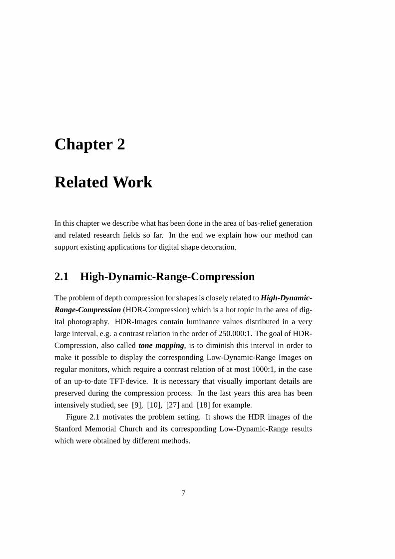
Figure 2.1 motivates the problem setting. It shows the HDR images of the

Stanford Memorial Church and its corresponding Low-Dynamic-Range results

which were obtained by different methods.

7

8 CHAPTER 2. RELATED WORK

Figure 2.1: Original HDR-image (courtesy of Paul Debevec) (left); result afterapplying the method of [27] (middle); outcome of the approach of [11] (right);the details in the windows are very well reproduced in both cases, but the floorand the steps in the right image look more natural; moreover the contrast in themiddle left and upper right part of the images is better enhanced by the method of[11]

Since Bas-relief generation has to ”squeeze”a shape into the available depth

range without destroying perceptually relevant features, it can be regarded as a

geometric pendant to tone mapping.

Our method mainly relies on the pioneering work of [11]. Their main idea

is to work in the gradient domain and manipulate the partial derivatives in a way

that large magnitudes are attenuated stronger than low ones. Therefore, they use

a multi-resolution approach. In the end, they recombine the gradient components

to the new low dynamic range image.

Nevertheless, an extension of this approach to range data is not straightfor-

ward because there are significant differences between features in digital images

and features on shapes. Moreover, HDR-images are more or less continuous,

whereas depth maps consist of a foreground and a background part which leads to

problems along an object’s silhouette. These discrepancies forced us to perform

some radical changes in order to adapt the method to our needs.

2.2. BAS-RELIEFS 9

2.2 Bas-Reliefs

The effect that bas-reliefs, viewed from an orthogonal vantage point, are almost

indistinguishable from a full 3D scene is called the bas-relief ambiguity. This

phenomenon is a matter of human perception which is studied in [3]. The authors

proof that there exists a 3-parameter family of transformation from a shape to a

corresponding bas-relief such that the shading and shadowing in both cases are

identical.

As long as a viewer only changes his perspective slightly around an orthogonal

view, the impression of a full relief remains. Once a certain vantage point is

exceeded, the flattening and also distortion are revealed.

If an object is recorded from several angles under unknown lighting condi-

tions, the bas-relief ambiguity will make it hard for a computer to resolve the

shape of this object, because the solution is not unique in general, unless assump-

tions about the surface properties are made. This problem constitutes an active

area of research in computer vision [2], [26].

In contrast to that, we exploit the existence of the bas-relief ambiguity because

we want to achieve exactly the opposite. Our aim is to create a shape which

is different from an original but exhibits the same appearance. The bas-relief

ambiguity justifies our motivation that for each model such corresponding shapes

do exist.

Currently, there are four works which directly address the challenge of gener-

ating reliefs with the help of computers.

In [7] this problem is studied for the first time. The authors present simple al-

gorithms to produce bas- and high-reliefs. They introduce the idea to work with a

view dependent height field from a given 3D scene. First, they generate the range

image by z-buffering and then a perspective transformation (reciprocally propor-

tional to the depth) is applied such that objects in the background are mapped to a

smaller z-range than those closer to the foreground. This results in a kind of per-

spective foreshortening. After that, a linear scaling is applied in order to receive

the appropriate range in the result. This is the very first work in this field and the

results are great for high-reliefs but unfortunately for bas-reliefs and especially

for high compression ratios it does hardly better than linear rescaling in terms of


feature preservation.

Then, for a long time this research area has completely been out of focus until

three works have appeared in the same year.

In [23] the authors describe a method to compute a bas-relief of a given mesh.

Therefore, they represent the shape in appropriate differential coordinates, then

they use a saliency measure [16] and combine it with a feature enhancing tech-

nique. In the end, the shape is rescaled and the bas-relief is reconstructed from the

corresponding differential coordinates.

Inspired by the results of [23], we developed an algorithm for range image

compression in a feature preserving way which is presented in [14]. It adapts the

main ideas of [11] to our shape processing purpose and operates in the gradient

domain. In this work, we have mainly been interested in keeping the surface

structure of an object perceivable in the generated depth compressed version. The

information about the surface structure is covered in the high frequencies of the

partial derivatives. So, we first split the image into its gradient components and

extract their high frequencies, which are then rescaled before we recombine them

to the depth compressed result. At this time, we have ignored the low frequencies.

The results of this method, look quite good but in some sense they seem unnatural

and exaggerated. This thesis is an extension of our earlier work. It addresses

some open drawbacks (see Section 3.3) and drastically improves the quality of

the outcomes.. Figure 2.2 contains a comparison.

The work of [28] provides a semi-automatic tool which assists an artist with

creating bas-reliefs. Their approach is also based on the ideas presented in [11]

and it works in the gradient domain too. A logarithmic attenuation function is

used in order to compress large gradients stronger than low ones. Then, they give

a user the possibility to treat several frequency bands in the new gradient image

individually. This requires the artist to adjust several weight-parameters. At first

glance, their approach seems to be quite similar to ours but it differs a lot in some

crucial points, as it will be discussed at the end of the next chapter.

These current works are an indication for the growing interest in this very

young research field.

2.3. VIRTUAL SHAPE DECORATION 11

Figure 2.2: Bas-relief of the armadillo and the lion vase model [1] achieved withthe apporach proposed in [23] (left), obtained by the algorithm of [14] (middle)and the result of the method presented in this thesis (right); compression ratio is2% in all cases

2.3 Virtual Shape Decoration

The area of virtual shape decoration covers several techniques, e.g. embossment,

engraving, carving or digital sculpting. Its aim is the generation of synthetic pieces

of art which cover the same styles, effects and impressions like their real world

pendants.

In [24] and [25] the authors provide a set of tools and an interactive shape

modeler which allows an artist to create synthetic embossments and wood cut-

tings. The drawback of this method is that the work is completely in the hand of a


user. This is time-consuming and the quality of the results largely depends on the

skill of the artist.

Another set of tools for synthetic carving is presented in [19]. Among in-

teractive carving their approach allows two and three dimensional input to deco-

rate shapes. The authors restrict themselves to implicit surfaces and explain that,

among other techniques, ray casting is used to compute depth data from a given

3D scene but the problem of how to compress this data to an appropriate size for

their purpose is not considered.

A computer based sculpting system for the creation of digital characters for

the entertainment industry is presented in [20]. They require 3D or range data

as input, then a user has several editing options to manipulate the outcome. For

their algorithm they use adaptively sampled distance fields [12] and exploit their

properties.

In the first case our algorithm can contribute by acting as a kind of preproces-

sor, such that range data of synthetic objects can be used to produce a template

which can then be further modified, rather than working from scratch. This could

improve the quality of the results and would lead to greater success for untrained

users. If a model should be carved into another virtual object, then our method

can be used to preserve more features in the outcome or even exaggerate them.

Once range data is used as input, we can support digital sculpting by requiring

less user interaction to produce similar or even better looking results.

Chapter 3

Gradient Domain Approach

In this chapter we describe the different phases of our gradient domain bas-relief

generation method. First, we give a global survey of the algorithm and then we

explain the purpose and the contribution of each step in detail. We illustrate those

effects using the armadillo model as an example.

Later in this chapter, we present several results which have been obtained with

the help of our approach. We inspect the influence of the user adjusted parameters

and investigate the performance. Finally, the algorithm is discussed and compared

to other recent bas-relief generation methods.

3.1 Algorithm

3.1.1 Overview

The main idea of our algorithm is to work in the gradient domain like it was

proposed in [11]. The workflow shown in Figure 3.1 describes the interplay of

the different steps.

After having read a given range image I(x, y), it is split into its gradient com-

ponents Ix and Iy. A problem which naturally arises when working with depth

maps forces us to perform a thresholding in order to get rid of boundary artifacts;

this leads to Ix and Iy. Then, an attenuation function is applied in order to com-

press the interval size, and we receive Ix and Iy. The following unsharp masking

step allows a user to treat the high frequency band individually. So, an artist can

13

14 CHAPTER 3. GRADIENT DOMAIN APPROACH

Figure 3.1: Survey of the different algorithm phases

decide whether small details should be boosted or not present in the result at all.

At this stage, the new gradient components Jx and Jy of the intermediate result

are already computed. Solving a Poisson problem lets us reconstruct J with the

help of its partial derivatives. Although this range image now exhibits a very small

depth, its interval range is adapted by a global linear scaling in order to make it

suit to the given purpose, and so we receive the final bas-relief J .

3.1.2 Background Detection

An input file which has been generated with 3D scanners typically contains a

binary background mask in addition to the height data I(x, y) itself. In other cases,

e.g. ray casted or z-buffered shapes, such a binary mask B(x, y) is extracted after

having read the range image data:

B(i, j) =

{0, if I(i, j) = δ

1, else(3.1)

Here, δ represents the default background value of the depth map.

It is important that background information does not influence the further com-

putation of the foreground data. This mask helps us to distinguish which part a

pixel belongs to and is used to normalize the result in the end. Figure 3.2 shows the

initial range image and the extracted background mask for the armadillo model.

3.1. ALGORITHM 15

Figure 3.2: Initial color-coded shape (left); most salient parts are indicated by redand those further to the background are colored blue; the value range is 300 at thatstage; corresponding binary background mask (right)

3.1.3 Decomposition

In order to work in the gradient domain the partial derivatives Ix and Iy of the

height field have to be computed. They are obtained with the help of a differential

quotient in two dimensions:

Ix(i, j) ≈I(i + h, j) − I(i, j)

h(3.2)

Iy(i, j) ≈I(i, j + h) − I(i, j)

h(3.3)

In our discrete case it holds that h = 1, and so the equations shown above collapse

to a finite forward difference:

Ix(i, j) ≈ I(i + 1, j) − I(i, j) (3.4)

Iy(i, j) ≈ I(i, j + 1) − I(i, j) (3.5)

The fact that the background value is usually very different from the fore-

ground data leads to large peaks at the object’s boundary. In Figure 3.3 a 1D

signal is used to illustrate the problem.


Figure 3.3: 1D signal with boundary and default background value (left) and cor-responding first derivative obtained by finite difference (right)

In the two dimensional case, which is shown in Figure 3.4, a viewer can only

see a thin line (exactly one pixel of width) of large values along the silhouette and

all other information inside is close to 0 relative to these discontinuities. Keeping

such jumps results in a larger depth interval and the problem that small details

will hardly be perceivable in the result. Furthermore, these peaks lead to artifacts

during the high frequency computation.

In general, this problem cannot be solved by adapting the background value in

advance. So, we have to modify Ix and Iy in a way that the outliers are eliminated.

Figure 3.4: Gradient components of the armadillo model; X-gradient (left) andY-gradient (right); both exhibit a very large value range

3.1. ALGORITHM 17

3.1.4 Thresholding

This step detaches high values form the gradient images. Therefore, a user defined

parameter τ is introduced and all pixels whose absolute value is greater than this

threshold are set to 0. First, we generate a binary threshold mask T :

T (X, i, j) =

{1, if |X(i, j)| ≤ τ

0, else(3.6)

This mask is then used to cut out the corresponding entries. The �-operator

means component-wise multiplication in this case:

Ix = T (Ix) � Ix (3.7)

Iy = T (Iy) � Iy (3.8)

Note, that this method also affects larger jumps on the object’s surface. If τ

is chosen too high, then larger gradients will form the result and smaller details

will hardly be visible. If it is chosen too small, then flat artifacts can arise during

the reconstruction step, because important information is lost. So, this parameter

gives an artist the opportunity to steer which kind of gradients should be removed

(respectively remain), but conceals the risk of cutting off too much. The influence

that τ has on the outcome is further discussed in the result section.

Neither the pixels in the background nor the peaks along the silhouette and

on the object’s surface may contribute to the further processing. Therefore we

construct a binary combined mask C with the help of B and T for which a pixel is

set to 1 if and only if it is equal to 1 in the background mask and in both threshold

masks:

C = B � T (Ix) � T (Iy) (3.9)

Figure 3.5 illustrates the effect of this step on the armadillo model. It shows

the thresholded gradient images Ix and Iy as well as the corresponding combined

mask C.


Figure 3.5: (left and middle) Thresholded X- and Y-gradient of the armadillomodel; in this example τ = 5; note that the details of the armadillo are nowvisible in contrast to Figure 3.4 and the interval size changes drastically accordingto τ ; (right) combined binary mask; the positions of detached pixels are markedin the mask, this holds especially for the jaw in this example

3.1.5 Attenuation

Up to now, we have produced continuous gradient images.

By definition, attenuation is the reduction in amplitude and intensity of a sig-

nal [29]. In practice, this means that values of larger magnitudes have to be

diminished stronger than small entries. This relative convergence leads to a com-

pression of the remaining interval size by keeping the appearance of the signal.

There is a number of different ways in order to achieve attenuation. We have

decided to apply the function proposed in [11]. Therefore, we first construct a

weight matrix A:

A(X, i, j) =

0, ifX(i, j) = 0

a|X(i,j)|

·(

|X(i,j)|a

)b

, else(3.10)

Then, these weights are applied by component-wise multiplication and we

obtain the thresholded and attenuated gradient components Ix and Iy:

Ix = A(Ix) � Ix (3.11)

Iy = A(Iy) � Iy (3.12)

Note, that the gradients in the background and those which were detached

before remain unchanged, because zero entries are mapped to zero entries again.

3.1. ALGORITHM 19

This method needs two parameters a and b. It has the effect that absolute val-

ues above a are attenuated and those below are slightly enhanced. At first glance,

this magnification seems to be counterproductive for the purpose of compression

but it comes up with the benefit of preserving small entries by boosting them in

that way. Figure 3.6 shows the graph of the attenuation function.

Figure 3.6: The parameter ”a”of the attenuation function marks the position of the1-intersection, it is 10 in this particular example; the parameter ”b”steers how fastthe weights approach the x-axis, here it is 0.9

If a depends on the interval-constitution then the whole function will be adap-

tive because it returns different weights for the same value if it is contained in

different intervals. For all images in the following, the reference value a is chosen

10 % of the average absolute value of all unmasked pixels in X. The parameter

b which affects the compression ratio is fixed at 0.9 for all results shown in this

thesis. So, basically this attenuation step does not need any user interaction.


3.1.6 Unsharp Masking

If a user wants to achieve a very high compression ratio, then it is likely that fine

details will hardly be perceivable in the result. The slight enhancement from the

previous step is not sufficient to overcome this problem in general. The small

features are covered in the high frequencies of the signal and that’s why the high

frequency part has to be boosted in order to emphasise the fine details and keep

them up through the procedure.

Therefore, we use the concept of unsharp masking, which is a classical tech-

nique to sharpen images that was even applied in historical photography around

the 1930’s [29]. Today unsharp masking is widely used in many areas throughout

computer graphics e.g. to enhance features in digital images [17] or meshes [13]

[8]. The main idea is to create a smoothed version of a signal and subtract it from

the original in order to obtain the high frequent part, which is then linearly scaled

by a user specified factor and added back to the low frequency component.

If the background pixels and those which have been thresholded before con-

tribute to the blurring, then some pixels in the low frequent part will be of a mag-

nitude which is too small, because there is a number of undesired 0-valued entries

in their neighbourhood. Moreover, some of the masked pixels would be given

an unpredictable value different from 0, since the smoothing kernel reaches the

foreground pixels. Both cases lead to peaks in the extracted high frequency part,

because the smoothed version of the signal exhibits values which are either higher

or lower than expected. Such discontinuities will cause artifacts in the result, so

we have to address this problem.

The most important step is the following discrete convolution. For the smooth-

ing itself we use a 2D Gaussian filter Gσ of standard deviation σ and correspond-

ing kernel size. Here, m and n are the indices of the filter in x respectively y

direction and C represents the combined binary mask obtained from Equation

3.9:

Blurσ(X, i, j) =

0, ifC(i, j) = 0P

m,nGσ(m,n)C(i−m,j−n)X(i−m,j−n)

P

m,nGσ(m,n)C(i−m,j−n)

, else(3.13)

3.1. ALGORITHM 21

The main idea of this function is that it only considers unmasked pixels in a

neighbourhood for the weighted averaging, and like in the previous step it leaves

the masked pixels untouched. The denominator is used for normalization, so that

the weights which are actually used sum up to 1.

If we use the above mentioned function in our special case, we can go on like it

is intended by regular unsharp masking. The signals are split into two components

Low and High, whereas we apply another slight smoothing to the high frequent

part in order to prevent occurring noise. After that, the weight of the high frequent

part is modified and it is added back to obtain the new partial derivatives of the

depth compressed range image, called Jx and Jy:

Low(X) = Blurσ1(X) (3.14)

High(X) = Blurσ2(X − Low(X)) (3.15)

Jx = Low(Ix) + α · High(Ix) (3.16)

Jy = Low(Iy) + α · High(Iy) (3.17)

The parameter σ1 decides how the signal is decomposed; in our examples the

value ranges from 2 to 5. In contrast to that, σ2 only serves to diminish noise and

is chosen 1 for all the results in this thesis. The new relation between the high

and low frequencies is steered by the parameter α > 0 which it depends on the

desired compression ratio or the intention of the artist. α = 1 leaves the balance

unchanged, α > 1 enhances the high frequencies whereas α < 1 impairs them.

The higher the compression, the higher α has to be set in order to keep the small

details up.

We want to accentuate that the second smoothing with σ2 is not essential.

Strictly spoken, this slight modification even destroys the idea of unsharp masking

because we only boost a part of the high frequencies since the highest ones are

eliminated. Nevertheless, experiments have shown that the results exhibit some

noise in regions with a small number of features and that the details appear to be

unnaturally sharp if the second blurring is omitted.

Figure 3.7 contains the enhanced gradient images Jx and Jy of the armadillo

model.


Figure 3.7: Intermediate result after unsharp masking; new X-gradient (left) andY-gradient (right); compare to Figure 3.5; here α = 6, σ1 = 4 and σ2 = 1

3.1.7 Poisson Problem

The results of the last step represent the new gradient components of the bas-relief.

So far, their discontinuities have been removed, they have been compressed and

their high frequencies have been boosted.

Now, we reconstruct the depth compressed range image J from its modified

gradient G =[

Jx

Jy

]. Since the partial derivatives have been manipulated, G is

not integrable anymore, in general. Therefore, we use an optimization process in

order to find a function whose derivative is closest G in a least square sense, like

it was proposed in [11] and [28]:

J(x, y) = arg minJ

∫ ∫||∇J(x, y) − G(x, y)||2dxdy (3.18)

Whereas, ∇ =

[∂

∂x∂

∂y

]represents the vector of partial derivatives.

Reformulating the equation shown above leads to the Poisson equation:

∆J = divG (3.19)

Here, ∆ = ∇2 = ∂2

∂x2 + ∂2

∂y2 denotes the Laplace operator, and div = ∂∂x

+ ∂∂y

stands for the divergence operator.

Adapted to our discrete case this means that the Laplacian of J is given by the

3.1. ALGORITHM 23

sum of the partial derivatives of G. Due to the discrete case which we are in, they

are obtained by a finite difference again like in Chapter 3.1.3, but here it has to be

the backward difffernce in order to produce a central difference like it is defined

for the Laplacian:

∆J =∂Jx

∂x+

∂Jy

∂y(3.20)

= Jxx + Jyy (3.21)

Jxx(i, j) ≈ Jx(i, j) − Jx(i − 1, j) (3.22)

Jyy(i, j) ≈ Jy(i, j) − Jy(i, j − 1) (3.23)

(3.24)

Now, the task is to compute a function J whose Laplacian is equal to the

right hand side of Equation 3.24. The solution to this Poisson equation is a well

known and well studied problem and there are standard techniques to address it,

so it should not be discussed in detail here. One has to solve a sparse system of

linear equations and therefore the Laplace matrix itself and a boundary is required.

In our case, the boundary is given by the default background value. As further

reading we recommend [4].

This step lets us recombine both partial derivatives, and so it brings us back

form the gradient domain to a height field (spatial domain).

3.1.8 Post Processing

So far, we have produced a range image which exhibits a greatly reduced depth

interval size. Small features are preserved because the relation between high and

low frequencies has been adapted by unsharp masking.

The above mentioned parameters τ , σ1, σ2 and α lead to a compression ratio

which is unknown in advance. In order to obtain the desired depth range, we

introduce a global linear scaling factor λ > 0 which makes the bas-relief suit to


the specific purpose. This bas-relief is called J .

λ =desired ratio

achieved ratio(3.25)

J = λ · J (3.26)

Then, we normalize the result with the help of the binary background mask B,

in a way that it ranges from 0 to a certain positive amount, whereas the background

pixels are set to 0.

Finally, we map our depth compressed height field to a regular triangulated

grid of appropriate resolution in order to visualize it as a three dimensional sur-

face. That means that the z-value of each vertex is set to the height of the cor-

responding pixel. The underlying connectivity of the vertices leads to a mesh

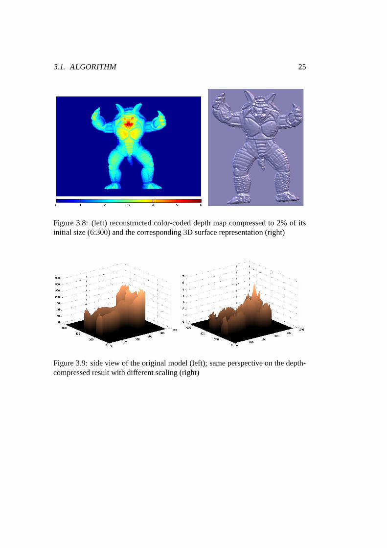
representation of the bas-relief. The outcomes are shown in Figure 3.8.

The careful reader might realize that the color distribution in the left part of

Figure 3.8 is very different compared to the one in Figure 3.2. In the original

the claws and the nose of the armadillo are almost on the same level whereas this

relation is heavily distorted in the result because the nose is much more salient

than the claws which, are even further to the background then the breast. In the

right image of Figure 3.8 such an effect is not perceivable because, on the one

hand it shows an almost orthogonal vantage point, and on the other hand these

differences on the surface are only visible if a very small scaling is applied to the

z-axis, since it is very flat. Another viewpoint and a different scaling reveal the

distortion, see Figure 3.9.

3.1. ALGORITHM 25

Figure 3.8: (left) reconstructed color-coded depth map compressed to 2% of itsinitial size (6:300) and the corresponding 3D surface representation (right)

Figure 3.9: side view of the original model (left); same perspective on the depth-compressed result with different scaling (right)


3.2 Results

In this section we present several results which demonstrate the potential of our

algorithm. We inspect the influence which the user adjusted parameters have on

the outcome and analyze the speed of this approach.

In Figure 3.10 we present different views on the bas-relief which corresponds

directly to the result of the last chapter. Note the preservation of the fine details

and the very small height.

More results for models of different size and complexity with varying com-

pression ratios are shown in Figure 3.11 and 3.12.

Figure 3.10: (top row) For the lower leg one can recognize the fine surface struc-ture as well as the nails; the parts of the mail on the upper leg and the differentmuscles around the stomach are very well distinguishable; the claws and the de-tails on the inner part are greatly preserved; (bottom row) side view of originalrange image and three different perspectives on the result after compressing it to2% of its initial extent

3.2. RESULTS 27

Figure 3.11: (top row) original Stanford dragon model [15] and its compressedversion (ratio of 1%); (bottom row) an ornament [1] and its corresponding bas-relief compressed to 2% of its former depth, note the preservation of the order, aviewer can recognize the overlapping levels of the model and knows which part isabove or behind the other one


Figure 3.12: a range image of a Buddhistic statue [5] (left) and the depth com-pressed model on the right (2%); note how well the low frequent features likeeyelids nose or mouth and the very high frequent structure on the head are pre-served at the same time

3.2.1 Parameters

Figure 3.13 shows the influence of the threshold parameter τ . If the value for τ

is too high, then discontinuities on the object’s surface will be preserved at the

expense of the visibility of small details. A small value for τ can lead to large

masked areas which make it hard to reconstruct the range image properly. Hence,

a meaningful setting of the threshold is required in order to find a balance between

the preservation of visually relevant details and continuity of the result.

The following two figures demonstrate the contribution of the unsharp mask-

ing step. The bas-reliefs in Figure 3.14 are produced using different values for σ1

which cause a different degree of smoothness in the outcome. Figure 3.15 demon-

strates the influence of α which steers the new relation between the high- and low

frequency part.

3.2. RESULTS 29

Figure 3.13: combined masks (top row) and corresponding results (bottom row)for τ = [75, 5, 1] from left to right (σ1 = 4, σ2 = 1, α = 6); in the left images onecan see that all inner pixels are taken into account (no difference to backgroundmask) which leads to an exaggeration of the jaw an the claws whereas the visibilityof the fine structure is impaired; the small features in the right part are betterpreserved but the loss of too much information on the coarse structure leads to flatartifacts; this holds especially for the silhouette, the jaw and the claws here; τ = 5leads to a meaningful relation


Figure 3.14: σ1 = 15 (left); σ1 = 10 (middle); σ1 = 2 (right); for large valuesof σ1 the high frequent features are still visible but they appear to be blurred;smaller values emphasise the details but the ridges are very sharp; compare thesmoothness of the reflections along the transitions of the stomach and the breastpart; in all cases τ = 5, σ2 = 1, α = 6

Figure 3.15: from left to right α = [20, 1, 0.2] (τ = 5, σ1 = 4, σ2 = 1); theseimages show that one can exaggerate the small details (high reflections arounddetails) by choosing a high boosting factor; for the case of α = 1 it is neutraland the features are visible but very flat (almost no reflections), this correspondsto a result for which only thresholding and attenuation are applied; impairing thehigh frequencies leads to an even more schematic appearance of the whole model(right)

3.3. DISCUSSION 31

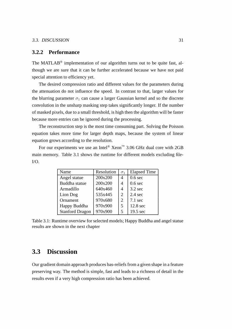
3.2.2 Performance

The MATLAB® implementation of our algorithm turns out to be quite fast, al-

though we are sure that it can be further accelerated because we have not paid

special attention to efficiency yet.

The desired compression ratio and different values for the parameters during

the attenuation do not influence the speed. In contrast to that, larger values for

the blurring parameter σ1 can cause a larger Gaussian kernel and so the discrete

convolution in the unsharp masking step takes significantly longer. If the number

of masked pixels, due to a small threshold, is high then the algorithm will be faster

because more entries can be ignored during the processing.

The reconstruction step is the most time consuming part. Solving the Poisson

equation takes more time for larger depth maps, because the system of linear

equation grows according to the resolution.

For our experiments we use an Intel® Xeon™ 3.06 GHz dual core with 2GB

main memory. Table 3.1 shows the runtime for different models excluding file-

I/O.

Name Resolution σ1 Elapsed TimeAngel statue 200x200 4 0.6 secBuddha statue 200x200 4 0.6 secArmadillo 640x460 4 3.2 secLion Dog 535x445 2 2.4 secOrnament 970x680 2 7.1 secHappy Buddha 970x900 5 12.8 secStanford Dragon 970x900 5 19.5 sec

Table 3.1: Runtime overview for selected models; Happy Buddha and angel statueresults are shown in the next chapter

3.3 Discussion

Our gradient domain approach produces bas-reliefs from a given shape in a feature

preserving way. The method is simple, fast and leads to a richness of detail in the

results even if a very high compression ratio has been achieved.


The reader may ask why the work in the gradient domain is necessary since

almost all operations used are linear. The crucial point is the thresholding which

helps to ignore larger jumps on the objects surface. The result of attenuating,

unsharp masking and linear rescaling in the spatial domain is absolutely identical

to the outcome shown in 3.13 for the reference value τ = 75 where the visibility

of the small features is impaired because the discontinuities around the jaw are

kept.

The distortion described in Section 3.1.8 is caused by the interplay of thresh-

olding and the solution of the Poisson equation for reconstruction. It would arise

even if no attenuation, unsharp masking or linear rescaling were performed. In our

special case such a distortion is desired because it supports the correct impression

of the model from an orthogonal vantage point like it is intended for bas-reliefs.

In [28] the authors use a logarithmic weighting function for attenuation, which

needs one parameter to steer the compression ratio. The problem with this ap-

proach is that the weight only depends on the absolute value of a pixel. This

means it returns the same result for a specific magnitude, disregarding its relation

to the other entries. Suppose we are given two very different models as input. The

thresholding step can cause gradient intervals of the same size for both models

although the distribution of values inside of them is very different. If we used log-

arithmic weights, then the values in both intervals would be treated exactly in the

same way. This is why we apply the function proposed in [11] which individually

adapts to different intervals.

Another difference to the approach presented in [28] is that it gives a user the

possibility to decompose the signal into an arbitrary number of different frequency

bands, which can then be weighted individually. On the one hand this leads to

more artistic control and even allows stop-band-filtering like it is described in

[13] but on the other hand it requires the user to find meaningful weights by trial

and error. Our method is limited to two different frequency bands, because we

used the approach presented in [17] and [8]. This means that stop-band-filtering

is not possible, but we can produce good looking results in a much more user

friendly, simpler and faster way.

As mentioned earlier, the method introduced in [7] is not applicable for high

compression ratios because it scales down globally once a height field is gen-

3.3. DISCUSSION 33

erated. This means that, if the range image is compressed too much, then the

preservation of small features will be similar to the one achieved by naive linear

rescaling. In contrast to that, our algorithm preserves fine details by boosting the

high frequencies and locally taking into account the constitution of each neigh-

bourhood.

This thesis is an extension of our earlier work [14] in which we only concen-

trated on the high frequencies and ignored the low ones. This has caused several

problems in areas which exhibit only a small number of features, e.g. spherical

parts. Depending on the parameters, these regions have either been noisy or com-

pletely flattened. Hence, we include the low frequencies now, and obtain results

which look much more natural because the convexity in such areas is preserved.

Moreover, in [14] we have used global blurring, which has led to exaggerated

large and sharp ridges and other undesired artifacts, because it introduces discon-

tinuities at locations where entries have been thresholded, as it is explained in

Section 3.1.6. Currently we apply the discrete convolution function described in

Equation 3.13, in order to prevent those peaks.

Chapter 4

Laplacian Domain Approach

For the gradient domain approach it is necessary to compute the Laplacian of

the range image in order to get back to the spatial domain. That’s why we have

thought of manipulating the Laplacian directly. To the best of our knowledge, for

the purpose of depth compression of shapes this has not been done before.

The idea behind each step is the same like in Chapter 3, but the effects which

they have are different because the Laplacian and the gradient represent different

properties of the model. In order to not repeat what has been described before,

we keep this chapter more technical and only demonstrate the differences to the

gradient domain approach. Therefore we use the armadillo model here again.

Let the height field I(x, y) be given and the binary background mask B(x, y)

be extracted like described in Section 3.1.2. We begin with the computation of

the Laplacian ∆I of the range image. By definition ∆I is the sum of the second

derivatives in both dimensions.

∆I = Ixx + Iyy (4.1)

Ixx(i, j) ≈I(i + h, j) − 2I(i, j) + I(i − h, j)

h2(4.2)

Iyy(i, j) ≈I(i, j + h) − 2I(i, j) + I(i, j − h)

h2(4.3)

Since the range images are discrete it holds again that h = 1 in our case.

35

36 CHAPTER 4. LAPLACIAN DOMAIN APPROACH

Reformulating the above mentioned equations under consideration of this fact

leads to the following approximation:

∆I ≈

0 1 0

1 −4 1

0 1 0

⊗ I (4.4)

This 3x3 filter and the large differences between foreground and background

data lead to the fact that the peaks along the silhouette have a width of 2 pixels

now. Like in Section 3.1.4 we use thresholding with reference value τ to eliminate

those outliers and obtain ∆I . B(x, y) is extended to the combined mask C(x, y)

accordingly.

∆I(i, j) =

{1, if |∆I(i, j)| ≤ τ

0, else(4.5)

Figure 4.1 shows the Laplacian of the armadillo depth map before and after

thresholding.

Figure 4.1: Initial Laplacian of the armadillo range image (left) and the corre-sponding thresholded version (right)

Then we apply the attenuation function described in Section 3.1.5 to get ∆I ,

whereas the parameter a depends on the signal constitution and b is chosen 0.9

again.

37

∆I(i, j) =

0, if∆I(i, j) = 0

a

|∆I(i,j)|·(

|∆I(i,j)|a

)b

, else(4.6)

This step is followed by unsharp masking which boosts the high frequencies

and produces the new Laplacian ∆J for the bas-relief. Therefore, the discrete con-

volution Blurσ, which has been introduced in Section 3.1.6, is used. We omit the

additional smoothing of the high frequency component here because the visibility

of very fine details in the result is impaired even for a slight blurring. The noise

reduction which could be achieved by the second smoothing is hardly perceivable

as experiments have shown, and so it plays a minor role here.

Low(∆I) = Blurσ(∆I) (4.7)

High(∆I) = ∆I − Low(∆I) (4.8)

∆J = Low(∆I) + α · High(∆I) (4.9)

The intermediate results after attenuation and unsharp masking are presented

in Figure 4.2.

Figure 4.2: Thresholded and attenuated signal (left); corresponding image afterunsharp masking (σ = 4, alpha = 100)


Due to the fact that we have produced a new Laplacian directly, the recon-

struction of J can be done by solving the Poisson equation ∆J = f immediately.

Figure 4.3 contains the reconstructed, rescaled and normalized height field in a

color-coded way as well as the corresponding surface representation (see Section

3.1.8 for details).

Figure 4.3: Color-coded bas-relief (left) and its surface representation (right)

4.1 Results

The color distribution in the left part of Figure 4.3 shows that the generated bas

relief exhibits a heavy bending. This is the counterpart to the distortion in the

gradient domain approach. The bending is caused by the thresholding step and

the solution of the Poisson equation for reconstruction. In our case this bending is

undesired because it elevates the center of an object too far from the background.

Figure 4.4 contains different views on the bas-relief.

In Figure 4.5 we compare two more results of this approach with those ob-

tained by the gradient domain method.

The values for the threshold τ and the blurring parameter σ are similar to the

ones for the gradient method (τ ≈ 5, σ ≈ 4 ), whereas the enhancement factor α

is larger than 100 for the results presented in this chapter.

4.1. RESULTS 39

Figure 4.4: All three views show that the middle of the bas-relief is significantlyelevated, whereas the ears and feet stand out only slightly from the background.Especially the tail which normally belongs to the background plane is affected bythis undesired rising towards the object’s center


Figure 4.5: Happy Buddha model [15] compressed with gradient domain ap-proach (left) and the corresponding bas-relief obtained by Laplacian method (mid-dle); depth compressed version of a kneeling angel statue [5] achieved with gradi-ent (top right) and Laplacian algortihm (bottom right); all models are compressedto 2% of their former spatial extend; note that the ends of the rope as well asthe rope itself, the chain, the contours of the coat and the facial expression canbe recognized for the Buddha model; the preservation of the fine structure at thewings and the hair are striking in the angel example; The Laplacian images coverall these details but the overall appearance of the gradient domain results is moreplastic and natural

4.2. DISCUSSION 41

4.1.1 Performance

Due to the fact that we only work on one image (Laplacian), we achieve an enor-

mous increase in speed, compared to the work on two different components.

Thresholding, attenuation and unsharp masking have to be applied only once,

which saves almost half of the runtime. The computation of the Laplacian only

requires one convolution instead of four finite differences.

Table 4.1 shows the computation times for the results presented in this section

(file-I/O excluded; Intel® Xeon™ 3.06 GHz dual core).

Name Resolution σ Elapsed TimeAngel 200x200 4 0.3 secArmadillo 640x460 4 2.0 secHappy Buddha 970x900 5 7.5 sec

Table 4.1: Runtime overview for selected models

4.2 Discussion

All in all, the feature preservation of this Laplacian algorithm is acceptable but the

appearance of the model in the final bas-relief is not as good as the results obtained

by the gradient domain approach. For high compression ratios the bending itself

is not visible from an orthogonal vantage point, but if the compression is relatively

low, then the reflections on the surface will reveal this deformation.

This Laplacian domain approach is an extension of an algorithm which is

pretty novel itself, hence the current state is only preliminary. A different method

to overcome the boundary problem at the object’s silhouette is required in order

to produce evenly flat results. We are still searching for an appropriate solution

but we could not find a satisfying one until the deadline for this thesis.

The virtual results in both of our approaches look very promising, but there

will be two grave practical problems if these results should be ”brought to real

life” with the help of a CNC machine, a milling device, or a laser carver.

(1) The tools which are used e.g. by a milling device, have a certain spatial

extend so that very small details either cannot be produced or will be destroyed

again during the process.


(2) The crucial point is the fact that our generated height fields are discrete.

A CNC machine needs to know the transition from one entry to the next. These

can be e.g. linear, parabolic, cubic or a circular arc of given radius. So, if our

depth compressed range images serve as input, one has to decide in advance which

transition should be applied where; or a spline curve has to be fitted through all

discrete points of a row for each column. But then, it cannot be guaranteed that

the effects and details which are visible in the synthetic results also arise on the

material in the outcome.

The authors of [28] have produced a limestone sculpture but due to the above

mentioned reasons, it exhibits only a small number of coarse features compared

to their virtual results.

Chapter 5

Discussion & Conclusion

5.1 Discussion

The approach presented in [28] is currently the most flexible one for the genera-

tion of bas-reliefs. This method offers a number of possible artistic effects and the

user is given a lot of freedom, e.g one can use an arbitrary number of frequency

bands and change their relative weights. But this freedom requires either an ex-

perienced artist or a trial and error adjustment for the parameters in case of an

untrained user.

The gradient domain approach presented in this thesis is restricted in the num-

ber of possible artistic effects so far. Nevertheless, it produces bas-reliefs which

can at least compete with the ones achieved by the algorithm presented in [28], it

is reasonable fast and much more user friendly.

The method presented in [14] is, in some sense, a subset of our current gra-

dient domain algorithm. It focuses only on high frequencies which leads to either

slightly noisy or exaggerated results. Depending on the model or the artists inten-

tion this method is absolutely sufficient. Its advantages are the simplicity and the

higher speed.

The Laplacian approach from Chapter 4 is still under development. All in

all, the results are not yet satisfying but promising and they require only short

computation times. The look of the outcomes of the gradient algorithm is still

more natural than the one of the bas-reliefs generated by the Laplacian method.

43

44 CHAPTER 5. DISCUSSION & CONCLUSION

The pioneering work of [7] is not applicable if high compression ratios are

needed because then the feature preservation is hardly better than the one of linear

rescaling. Nevertheless their method is simpler and faster than any other approach

in this area.

5.2 Conclusion

In this thesis we have described a method which assists a user with the gener-

ation of bas-reliefs from a given shape. Furthermore, we have shown how this

approach, which operates on the gradient, can be raised to the Laplacian domain.

The artist has the possibility to steer the relative attenuation between coarse and

fine details in order to control their presence in the outcome. For an orthogonal

vantage point we can achieve arbitrary compression ratios and preserve visually

important details at the same time.

Due to the fact that this problem is related to High-Dynamic-Range-

Compression we have adapted several ideas from tone mapping to our purpose.

Our algorithm is simple, fast, easy to implement and independent of the model’s

complexity. Possible applications are any kind of synthetic or real world shape

decoration like embossment, engraving, carving or sculpting.

This is a very young and interesting research field which currently receives

more attention. The results in this area look very promising but there is still a

number of possible extensions.

5.3 Future Work

So far, the three dimensional scenes which are used as examples, only consist

of one object. For a very complex or even panoramic scene with many objects,

z-buffering from one perspective camera or orthogonal ray-casting can leads to

distortion, bending and other undesired artifacts. For a sequence of two dimen-

sional images this problem is e.g. studied in [21] and [22]. That’s why the use of

multi-perspective techniques constitutes a direction for future research. We expect

a huge difference between the results obtained by a regular one camera capturing

5.3. FUTURE WORK 45

of a scene and the outcomes achieved with a multi-view approach. It also offers

the opportunity to make hidden objects visible by having a camera pointing be-

hind an occluding object. Multiple viewpoints have been applied in paintings for

a very long time e.g. by Pablo Picasso. In our case multi-perspective methods

would give more respect to human perception on the one hand and provide many

more possible artistic effects on the other hand.

The design of a hybrid approach which keeps and enhances gradient details as

well as properties of the Laplacian and combines both methods is another possible

extension. Therefore, we want to improve the work in the Laplacian domain by

applying a different silhouette treatment.

Using and developing other techniques to extract and treat the frequency

bands, e.g. by multi-resolution methods, would give the user even more control

on the outcome and offer further artistic effects as well.

In contrast to that, we also think of reducing the user intervention by devel-

oping a quality measure which takes into account the properties of the generated

bas-reliefs and those of the original height field. This could help to introduce adap-

tive parameters for the functions used inside of our algorithm and hence make the

process more automatic.

46 CHAPTER 5. DISCUSSION & CONCLUSION

Bibliography

[1] AIM@SHAPE. AIM@SHAPE shape repository. http://shapes.aim-at-shape.net/.

[2] Neil Alldrin, Satya Mallick, and David Kriegman. Resolving the generalizedbas-relief ambiguity by entropy minimization. In IEEE Conf. on ComputerVision and Pattern Recognition, June 2007.

[3] Peter N. Belhumeur, David J. Kriegman, and Alan L. Yuille. The bas-reliefambiguity. Int. J. Comput. Vision, 35(1):33–44, 1999.

[4] Dietrich Braess. Finite Elements: Theory, Fast Solvers, and Applications inSolid Mechanics. Cambridge University Press, 2002. second edition.

[5] Richard J. Campbell and Patrick J. Flynn. A www-accessible 3D imageand model database for computer vision research. In Empirical EvaluationMethods in Computer Vision, K.W. Bowyer and P.J. Phillips (eds.), pages148–154, 1998. http://sampl.ece.ohio-state.edu/data/3DDB/index.htm.

[6] Richard J. Campbell and Patrick J. Flynn. Experiments in transform-basedrange image compression. In ICPR ’02: Proceedings of the 16 th Interna-tional Conference on Pattern Recognition (ICPR’02) Volume 3, page 30875,2002.

[7] Paolo Cignoni, Claudio Montani, and Roberto Scopigno. Automatic gener-ation of bas- and high-reliefs. Journal of Graphics Tools, 2(3):15–28, 1997.

[8] Paolo Cignoni, Roberto Scopigno, and Marco Tarini. A simple normal en-hancement technique for interactive non-photorealistic renderings. Com-puter & Graphics, 29(1):125–133, 2005.

[9] Paul Debevec and Erik Reinhard. High-dynamic-range imaging:Theory and applications. SIGGRAPH 2006 Course #5, 2006.http://www.siggraph.org/s2006/main.php?f=conference&p=courses&s=5.

47

48 BIBLIOGRAPHY

[10] Fredo Durand and Julie Dorsey. Fast bilateral filtering for the display ofhigh-dynamic-range images. In ACM Transactions on Graphics (Proc. SIG-GRAPH 2002), pages 257–266, 2002.

[11] Raanan Fattal, Dani Lischinski, and Michael Werman. Gradient domainhigh dynamic range compression. In ACM Transactions on Graphics (Proc.SIGGRAPH 2002), pages 249–256, 2002.

[12] Sarah F. Frisken, Ronald N. Perry, Alyn P. Rockwood, and Thouis R. Jones.Adaptively sampled distance fields: a general representation of shape forcomputer graphics. In ACM Transactions on Graphics (Proc. SIGGRAPH2000), pages 249–254, 2000.

[13] Igor Guskov, Wim Sweldens, and Peter Schroder. Multiresolution signalprocessing for meshes. In SIGGRAPH ’99: Proceedings of the 26th annualconference on Computer graphics and interactive techniques, pages 325–334, 1999.

[14] Jens Kerber, Alexander Belyaev, and Hans-Peter Seidel. Feature PreservingDepth Compression of Range Images. In SCCG ’07: Proceedings of the23rd spring conference on Computer graphics, April 2007. Winner 2nd bestSCCG ’07 paper award. Post-conference proceedings are in print.

[15] Stanford Computer Graphics Laboratory. Stanford 3D scanning repository.http://graphics.stanford.edu/data/3Dscanrep/.

[16] Chang Ha Lee, Amitabh Varshney, and David W. Jacobs. Mesh saliency. InACM Transactions on Graphics (Proc. SIGGRAPH 2005), pages 659–666,2005.

[17] Thomas Luft, Carsten Colditz, and Oliver Deussen. Image enhancement byunsharp masking the depth buffer. In ACM Transactions on Graphics (Proc.SIGGRAPH 2006), pages 1206–1213, 2006.

[18] Rafał Mantiuk, Karol Myszkowski, and Hans-Peter Seidel. A perceptualframework for contrast processing of high dynamic range images. In APGV’05: Proceedings of the 2nd symposium on Appied perception in graphicsand visualization, pages 87–94, 2005.

[19] Alexander A. Pasko, Vladimir Savchenko, and Alexei Sourin. Syntheticcarving using implicit surface primitives. Computer-Aided Design, Elsevier,33(5):379–388, 2001.

BIBLIOGRAPHY 49

[20] Ronald N. Perry and Sarah F. Frisken. Kizamu: a system for sculpting digitalcharacters. In ACM Transactions on Graphics (Proc. SIGGRAPH 2001),pages 47–56, 2001.

[21] Augusto Roman, Gaurav Garg, and Marc Levoy. Interactive design of multi-perspective images for visualizing urban landscapes. In VIS ’04: Proceed-ings of the conference on Visualization ’04, pages 537–544, 2004.

[22] Augusto Roman and Hendrik P. A. Lensch. Automatic multiperspective im-ages. In Rendering Techniques 2006: Eurographics Symposium on Render-ing, pages 161–171, 2006.

[23] Wenhao Song, Alexander Belyaev, and Hans-Peter Seidel. Automatic gen-eration of bas-reliefs from 3D shapes. In SMI ’07: Proceedings of the IEEEInternational Conference on Shape Modeling and Applications 2007, pages211–214, June 2007.

[24] Alexei Sourin. Functionally based virtual computer art. In SI3D ’01: Pro-ceedings of the 2001 symposium on Interactive 3D graphics, pages 77–84,2001.

[25] Alexei Sourin. Functionally based virtual embossing. The Visual Computer,Springer, 17(4):258–271, 2001.

[26] Ping Tan, Satya P. Mallick, Long Quan, David Kriegman, and Todd Zickler.Isotropy, reciprocity and the generalized bas-relief ambiguity. In IEEE Conf.on Computer Vision and Pattern Recognition, June 2007.

[27] Jack Tumblin and Greg Turk. Lcis: a boundary hierarchy for detail-preserving contrast reduction. In ACM Transactions on Graphics (Proc.SIGGRAPH 1999), pages 83–90, 1999.

[28] Tim Weyrich, Jia Deng, Connelly Barnes, Szymon Rusinkiewicz, and AdamFinkelstein. Digital bas-relief from 3D scenes. To appear in ACM SIG-GRAPH, August 2007.

[29] Wikipedia. Wikipedia, the free encyclopedia, 2007. http://en.wikipedia.org.

digital art of bas-relief sculpting - max-planck-institut f¼r informatik

Documents