digital filter structures and quantization effectsmocha-java.uccs.edu/ece5540/ece5540-ch06.pdf ·...
TRANSCRIPT

ECE4540/5540: Digital Control Systems 6–1
DIGITAL FILTER STRUCTURES AND
QUANTIZATION EFFECTS
6.1: Direct-form network structures
■ So far, we have assumed infinite-precision arithmetic when
implementing our digital controllers.
■ In reality, this is not possible.
• If we are lucky, we have the luxury of using floating-point arithmetic
(single- or double-precision).
• Often times, however, we will be restricted to fixed-point arithmetic
due to cost constraints.
• Both suffer quantization and overflow effects (although to a much
lower degree in floating-point implementations).
■ We look at these real-world considerations in this unit of notes.
Canonical network structures
■ The first consideration is how to implement a transfer function D(z) as
a “network” of primitive arithmetic operations: add, multiply, delay.
• For software realizations, the network corresponds to a flowchart
of the filter algorithm.
• For hardware realizations, the network describes the actual circuit
elements and their interconnection.
Lecture notes prepared by Dr. Gregory L. Plett. Copyright © 2017, 2009, 2004, 2002, 2001, 1999, Gregory L. Plett

ECE4540/5540, DIGITAL FILTER STRUCTURES AND QUANTIZATION EFFECTS 6–2
■ We will see that the performance of a digital implementation is
affected substantially by the choice of network structure.
■ There are a number of named “canonical” network structures for
implementing a transfer function, all of which have
• N delay elements,
• 2N (2-input) adders,
• 2N + 1 multipliers.
Direct-form II canonical form
■ To obtain the so-called “direct forms” of filter structure, we start with
the familiar LCCDE equation:N!
k=0
ak y[n − k] =
M!
m=0
bmx[n − m]
■ For convenience,
• Assume a0 = 1 (We can scale other ak and bk so that this is true).
• Assume N = M (We can always make some coefficients ak or bk
equal to zero to make this true).
■ Then, we get that the transfer function is equal to:
H(z) =
"Nn=0 bnz−n
1 +"N
n=1 anz−n=
1
1 +"N
n=1 anz−n×
N!
n=0
bnz−n.
■ We can realize this transfer function as a cascade of the denominator
dynamics followed by the numerator dynamics:
• The denominator dynamics implement a feedback path with
w[n] = x[n] − a1w[n − 1] − a2w[n − 2] − · · · − aNw[n − N ].
Lecture notes prepared by Dr. Gregory L. Plett. Copyright © 2017, 2009, 2004, 2002, 2001, 1999, Gregory L. Plett

ECE4540/5540, DIGITAL FILTER STRUCTURES AND QUANTIZATION EFFECTS 6–3
• The numerator dynamics implement a feedforward path with
y[n] = b0w[n] + b1w[n − 1] + b2w[n − 2] + · · · + bNw[n − N ].
■ We can realize the
overall transfer
function as shown:
x[n] y[n]w[n]+
+
++
+
+
z−1
z−1
z−1z−1
z−1
z−1
... ... ... ...
−a1
−a2
−aN
b0
b1
b2
bN
■ Notice that it is
possible to combine
the delay elements
and end up with a
simpler structure:
x[n] y[n]
+
+
+
+
+
+
z−1
z−1
z−1
...... ...
−a1
−a2
−aN
b0
b1
b2
bN
Lecture notes prepared by Dr. Gregory L. Plett. Copyright © 2017, 2009, 2004, 2002, 2001, 1999, Gregory L. Plett

ECE4540/5540, DIGITAL FILTER STRUCTURES AND QUANTIZATION EFFECTS 6–4
Transpose networks and the direct-form I canonical form
■ For any given network with a certain transfer function H(z), we can
generate a “transpose” of the network that has a different structure
but the same transfer function.
■ To obtain the transpose, follow these steps:
1. Start with the original network structure.
2. Replace all data flows with flows in the reverse direction.
3. Replace all summation nodes with branch nodes and all branch
nodes with summations.
4. Exchange x[n] and y[n].
x[n] y[n]
+
++
+
z−1
z−1
−a1
−a2
b1
b2
⇐⇒
x[n] y[n]+
+
+
z−1
z−1
−a1
−a2
b1
b2
■ If we take the transpose of a “Direct Form II” network (example on
left), we obtain a “Direct Form I” network structure (example on right).
■ The direct forms are simple to grasp and to implement, but have
some serious problems for high-order transfer functions.
■ Therefore, we look at several other canonical forms.
Lecture notes prepared by Dr. Gregory L. Plett. Copyright © 2017, 2009, 2004, 2002, 2001, 1999, Gregory L. Plett
ECE4540/5540, DIGITAL FILTER STRUCTURES AND QUANTIZATION EFFECTS 6–5
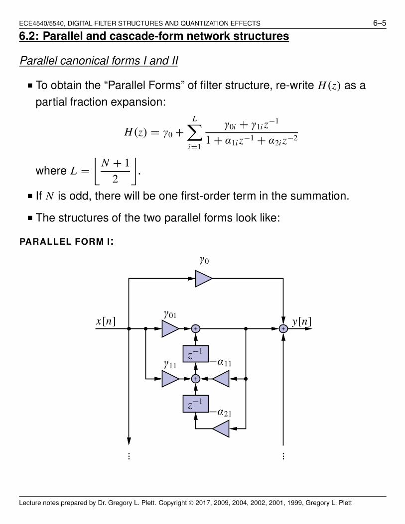
6.2: Parallel and cascade-form network structures
Parallel canonical forms I and II
■ To obtain the “Parallel Forms” of filter structure, re-write H(z) as a
partial fraction expansion:
H(z) = γ0 +
L!
i=1
γ0i + γ1i z−1
1 + α1i z−1 + α2i z−2
where L =
#N + 1
2
$.
■ If N is odd, there will be one first-order term in the summation.
■ The structures of the two parallel forms look like:
PARALLEL FORM I:
x[n] y[n]
+
++
z−1
z−1
......
γ0
γ01
γ11 −α11
−α21
Lecture notes prepared by Dr. Gregory L. Plett. Copyright © 2017, 2009, 2004, 2002, 2001, 1999, Gregory L. Plett

ECE4540/5540, DIGITAL FILTER STRUCTURES AND QUANTIZATION EFFECTS 6–6
PARALLEL FORM II:
x[n] y[n]++
+
+
z−1
z−1
......
γ0
γ01
γ11−α11
−α21
■ Again, these two forms are transposes of each other.
■ Also, they have the same number of delays, (two input) adders and
multipliers as the direct form implementations.
Cascade canonical forms I and II
■ To obtain the “Cascade Forms” of filter structure, re-write H(z) as a
product of second-order polynomials:
H(z) = b0
L%
i=1
1 + β1i z−1 + β2i z
−2
1 + α1i z−1 + α2i z−2
where L =
#N + 1
2
$.
■ If N is odd, there will be one first-order term in the product
(α2L = β2L = 0.)
Lecture notes prepared by Dr. Gregory L. Plett. Copyright © 2017, 2009, 2004, 2002, 2001, 1999, Gregory L. Plett
ECE4540/5540, DIGITAL FILTER STRUCTURES AND QUANTIZATION EFFECTS 6–7
■ The structures of the two cascade forms look like:
CASCADE FORM I:
x[n] y[n]. . .
++
+ +
++
z−1
z−1 z−1
z−1
b0
β11
β21
−α11
−α21
β1L
β2L
−α1L
−α2L
CASCADE FORM II:
x[n] y[n]. . .
+
++
++ +
++
z−1
z−1
z−1
z−1
b0
β11
β21
−α11
−α21
β1L
β2L
−α1L
−α2L
Lecture notes prepared by Dr. Gregory L. Plett. Copyright © 2017, 2009, 2004, 2002, 2001, 1999, Gregory L. Plett

ECE4540/5540, DIGITAL FILTER STRUCTURES AND QUANTIZATION EFFECTS 6–8
6.3: Implications of fixed-point arithmetic
■ Now that we have studied the most common filter structures, we
examine some of the real-life implications of using each structure.
■ There are tradeoffs: To determine which is best for a particular case,
there are four different factors that we must look at:
1. Coefficient quantization: The filter parameters are quantized such
that they are implemented in finite precision.
• Thus, the filter we implement is not exactly H(z), the desired
filter, but &H (z), which we hope is “close” to H(z).
• We can check whether &H(z) meets the control design
specifications, and modify it if necessary.
• The structure of the filter network has a drastic effect on its
sensitivity to coefficient quantization.
2. Signal quantization: Rounding or truncation of signals in the filter.
• It occurs during the operation of the filter and can best be viewed
as a random noise source added at the point of quantization.
3. Dynamic range scaling: We sometimes need to perform scaling to
avoid overflows (where the signal value exceeds some maximum
permitted value) at points in the network.
• In cascade systems, the ordering of stages can significantly
influence the attainable dynamic range.
4. Limit cycles: These occur when there is a zero or constant input,
but there is an oscillating output.
• Note that this arises from nonlinearities in the system
(quantization), since a linear system cannot output a frequency
different from those present at its input.
Lecture notes prepared by Dr. Gregory L. Plett. Copyright © 2017, 2009, 2004, 2002, 2001, 1999, Gregory L. Plett

ECE4540/5540, DIGITAL FILTER STRUCTURES AND QUANTIZATION EFFECTS 6–9
Binary representations of real numbers
■ There are two basic choices (with some variations) when
implementing non-integer numbers on a digital computer:
floating-point and fixed-point representation.
■ The fixed-point number system we will consider uses B + 1 bits:
x = Xm
'
−b0 +
B!
i=1
bi2−i
(
= XmxB.
■ We represent our number in binary as: xB = b0.b1b2b3 · · · bB.
• If b0 = 0, then 0 ≤ x ≤ Xm(1 − 2−B).
• If b0 = 1, then −Xm ≤ x < 0.
■ The “step size” of quantization is the smallest interval between two
quantized numbers = Xm2−B = $.
■ The fixed-point conversion error is: e = XmxB − x .
• For twos-complement truncation, −$ < e ≤ 0;
• For twos-complement rounding −$/2 < e ≤ $/2.
■ Floating point arithmetic splits the B + 1 bits into “mantissa” bits M
and “exponent” bits E such that
x = M2E where − 1 ≤ |M| < 1.
■ The exponent basically allows moving the decimal point (actually,
binary point) around in the number.
• With a fixed number of bits, floating-point representation allows
much greater dynamic range of the values it can represent.
Lecture notes prepared by Dr. Gregory L. Plett. Copyright © 2017, 2009, 2004, 2002, 2001, 1999, Gregory L. Plett

ECE4540/5540, DIGITAL FILTER STRUCTURES AND QUANTIZATION EFFECTS 6–10
• However, mathematical operations using floating point arithmetic
are much harder to implement.
◆ Hardware implementations require significantly more logic than
fixed-point implementations;
◆ Software implementations require significantly more operations,
so run much more slowly on the same processor.
■ Floating point arithmetic, although much harder to implement, poses
less of a problem to the digital filter designer than fixed point
arithmetic. Why?
EXAMPLE: Multiply 13/16 by 9/128.
■ Note,13
16=
)1
2+
1
4+
1
16
*× 20 and
9
128=
)1
2+
1
16
*× 2−3.
Fixed Point Floating Point
0.11010000 0.11010 000
×0.00010010 ×0.10010 101
110100000 = 0.01110101 101
110100000000 = 0.11101 100
= 0.0000111010100000
■ Comments:
• To store the result without losing precision, fixed point requires 12
bits but floating point requires 11 bits.
• Generally, floating-point results will be much better than fixed-point
results: double-precision math almost never gives problems to the
control engineer.
• Hardware DSP chips exist with floating point arithmetic built in.
Lecture notes prepared by Dr. Gregory L. Plett. Copyright © 2017, 2009, 2004, 2002, 2001, 1999, Gregory L. Plett
ECE4540/5540, DIGITAL FILTER STRUCTURES AND QUANTIZATION EFFECTS 6–11
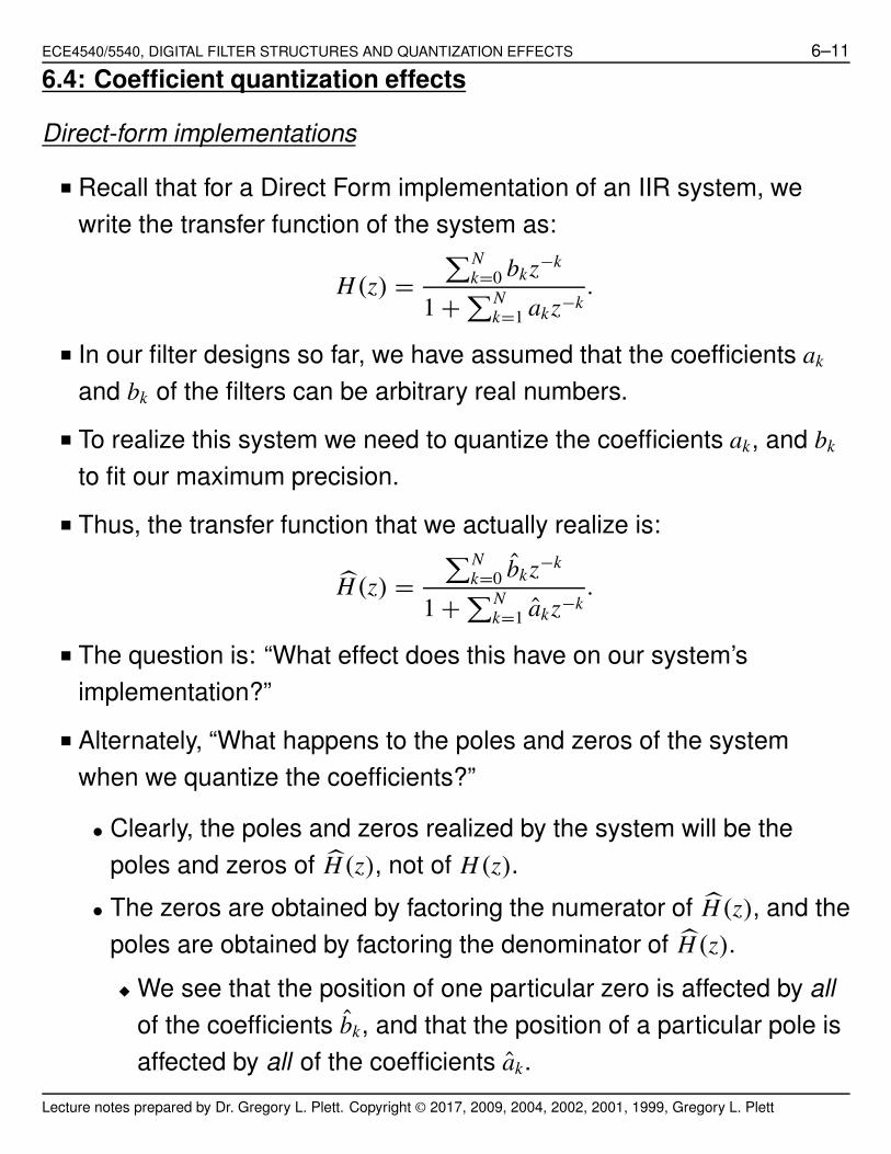
6.4: Coefficient quantization effects
Direct-form implementations
■ Recall that for a Direct Form implementation of an IIR system, we
write the transfer function of the system as:
H(z) =
"Nk=0 bkz−k
1 +"N
k=1 akz−k.
■ In our filter designs so far, we have assumed that the coefficients ak
and bk of the filters can be arbitrary real numbers.
■ To realize this system we need to quantize the coefficients ak, and bk
to fit our maximum precision.
■ Thus, the transfer function that we actually realize is:
&H(z) =
"Nk=0 bkz−k
1 +"N
k=1 akz−k.
■ The question is: “What effect does this have on our system’s
implementation?”
■ Alternately, “What happens to the poles and zeros of the system
when we quantize the coefficients?”
• Clearly, the poles and zeros realized by the system will be the
poles and zeros of &H(z), not of H(z).
• The zeros are obtained by factoring the numerator of &H(z), and the
poles are obtained by factoring the denominator of &H(z).
◆ We see that the position of one particular zero is affected by all
of the coefficients bk, and that the position of a particular pole is
affected by all of the coefficients ak.
Lecture notes prepared by Dr. Gregory L. Plett. Copyright © 2017, 2009, 2004, 2002, 2001, 1999, Gregory L. Plett

ECE4540/5540, DIGITAL FILTER STRUCTURES AND QUANTIZATION EFFECTS 6–12
◆ Thus, the effect of quantizing a specific coefficient is not isolated
in any way, but affects all poles or zeros in the function.
• A non-obvious result, which may be obtained with a little math, is
that closely clustered poles and zeros are most affected.
◆ Thus, narrow-band filters of any sort will be most strongly
changed.
QUESTION: So, what do we do about this?
ANSWER: We try to control the effect by localizing it using parallel or
cascade forms.
Coefficient quantization in a 2nd-order direct-form section
■ Cascade and parallel form implementations are made up of sections
of cascaded or parallel second-order direct-form filters.
■ Thus, to be able to see how coefficient quantization affects these filter
forms, we must first examine how it affects the 2nd-order section.
■ A second-order section with complex poles can be written as:
H(z) =1
(1 − re jθz−1)(1 − re− jθz−1)=
1
(1 − 2r cos θ z−1 + r2z−2).
■ These can be realized by the filter form
on the right.
■ The coefficients that require
quantization are: r cos θ and −r2.
■ Note: If both r2 < 1 and |r cos θ | < 1
then the system is stable.
x[n] y[n]
+
+
z−1
z−1
2r cos θ
−r2
Lecture notes prepared by Dr. Gregory L. Plett. Copyright © 2017, 2009, 2004, 2002, 2001, 1999, Gregory L. Plett

ECE4540/5540, DIGITAL FILTER STRUCTURES AND QUANTIZATION EFFECTS 6–13
QUESTION: Why do we quantize r cos θ and not 2r cos θ?
ANSWER: The multiply by 2 can be performed exactly by a shift register.
EXAMPLE: To see which poles can be implemented by this structure
using fixed-point arithmetic, suppose that four bits are available.
■ The coefficient structure is then a.bcd.
■ The positive values we can represent are:
0.001, 0.010, 0.011 . . . and 0.111. (We can
similarly compute negative values.)
■ So, r cos θ can take on these eight values,
and so can r2.
■ The intersection of allowable coefficients
give us the grid shown. 0 0.5 10
0.2
0.4
0.6
0.8
1
■ Observations:
• Narrow-band lowpass and narrow-band highpass filters are most
sensitive to coefficient quantization, and thus require more bits to
implement.
• Sampling at too high a rate is bad, since it pushes poles closer to
+1 (where the implementable pole density is smallest.)
• Sensitivity increases for higher-order direct form realizations.
Poles may end up outside the unit circle after rounding—unstable!
SOLUTION: Rather than implementing the second-order section in direct
form, we can choose an alternate network structure. For example, the
coupled form implementation is shown,
Lecture notes prepared by Dr. Gregory L. Plett. Copyright © 2017, 2009, 2004, 2002, 2001, 1999, Gregory L. Plett

ECE4540/5540, DIGITAL FILTER STRUCTURES AND QUANTIZATION EFFECTS 6–14
■ All of the coefficients of this
network are of the form r cos θ
and r sin θ .
■ The quantized poles are at in-
tersections of evenly spaced
horizontal and vertical lines.
0 0.5 10
0.2
0.4
0.6
0.8
1
x[n]
y[n]
w[n]
+
++
z−1
z−1r cos θ
r cos θ
r sin θ
−r sin θ
■ The price we pay for this improved pole distribution is an increased
number of multipliers: four instead of two.
Coefficient quantization in cascade- and parallel-form implementations
■ Cascade- and parallel-form realizations consist of combinations of
second-order direct-form systems.
■ However, in both cases, each pair of complex-conjugate poles is
realized independently of all the other poles.
■ Thus, the error in a particular pole pair is independent of its distance
from the other poles of the transfer function.
• For the cascade form, the same argument holds for the zeros
since they are realized as independent second-order factors.
Lecture notes prepared by Dr. Gregory L. Plett. Copyright © 2017, 2009, 2004, 2002, 2001, 1999, Gregory L. Plett

ECE4540/5540, DIGITAL FILTER STRUCTURES AND QUANTIZATION EFFECTS 6–15
◆ Thus the cascade form is generally much less sensitive to
coefficient quantization than the equivalent direct-form
realization.
• The zeros of the parallel form function are realized implicitly.
◆ They result from combining the quantized second-order sections
to obtain a common denominator.
◆ Thus, a particular zero location is affected by quantization errors
in the numerator and denominator coefficients of all the
second-order sections.
Lecture notes prepared by Dr. Gregory L. Plett. Copyright © 2017, 2009, 2004, 2002, 2001, 1999, Gregory L. Plett

ECE4540/5540, DIGITAL FILTER STRUCTURES AND QUANTIZATION EFFECTS 6–16
6.5: A2D/D2A signal quantization effects
■ In a typical digital filtering system there will be multiple sources of
signal quantization:
x(t) y(t)16-bit16-bit 32-bit
A2D DSP D2A
Quantization in the A2D conversion process
■ The first source of quantization error is the A2D conversion process.
■ We can quantize a signal in at least three different ways:
Rounding Trunc (twos-complement) Trunc (sign/mag)
−$
2
$
2−$ 0 −$ $
1
$
1
$ 1
2$
■ Rounding is the most common as it generally gives the best results.
■ The limits ±Xm of the quantized range might be selected using known
maximum values of a particular input signal.
Lecture notes prepared by Dr. Gregory L. Plett. Copyright © 2017, 2009, 2004, 2002, 2001, 1999, Gregory L. Plett

ECE4540/5540, DIGITAL FILTER STRUCTURES AND QUANTIZATION EFFECTS 6–17
■ Alternately, we might choose Xm based step size based on the
variance of the input signal.
• Assume a random input with variance σ 2 and zero mean.
• Then, we might let Xm = 4σ .
• Any sample greater in magnitude than 4σ gets quantized to the
closest bin (this is called “four sigma scaling”.)
• We could have chosen Xm = 3σ (three-sigma scaling), or even
Xm = 5σ (five-sigma scaling).
■ For a given number of quantizer bins (and therefore bits in the
representation), we are trading off quantization distortion in the
overload or granular regions.
Granular RegionOverload Region Overload Region
[k]
4σ 4σ■ The quantizer error e[n] is equal to
x[n] − xc(nT ). If we assume minimal
overload error, we can model e[n] as:
+xc(nT ) x[n]
e[n]
where e[n] is a random process having probability density function:
−$
2
$
2
1
$
■ The mean of the quantization error is:
Lecture notes prepared by Dr. Gregory L. Plett. Copyright © 2017, 2009, 2004, 2002, 2001, 1999, Gregory L. Plett

ECE4540/5540, DIGITAL FILTER STRUCTURES AND QUANTIZATION EFFECTS 6–18
E+e[n]
,=
- $/2
−$/2
e1
$de =
1
$·
e2
2
....$/2
−$/2
=1
$
/$2
8−
$2
8
0= 0.
■ The variance (power) of the quantization error is:
E+(e[n] − e[n])2
,=
- $/2
−$/2
e2 1
$de =
$2
12.
■ The quantization error e[n] and the quantized signal x[n] are
independent.
■ e[n] does depend on xc(nT ), but for reasonably complicated signals
and for small enough $, they are considered uncorrelated.
■ What is the signal to noise ratio?
■ The signal power is σ 2 =
)Xm
4
*2
(assuming four-sigma scaling). The
quantizer error power is E[e2] =$2
12.
■ Now, if we have B + 1 bits to store the quantized result, then there will
be 2B+1 bins of width $.
$ =2Xm
2B+1= Xm2−B
■ Therefore,
E[e2] =X2
m
12· 2−2B.
■ The signal to noise ratio is then
SNR = 10 log10
1 2Xm
4
32
X2m
12· 2−2B
4
= 10 log10
+22B
,+ 10 log10
+12/16
,
= 6.02B − 1.25 [dB]
Lecture notes prepared by Dr. Gregory L. Plett. Copyright © 2017, 2009, 2004, 2002, 2001, 1999, Gregory L. Plett
ECE4540/5540, DIGITAL FILTER STRUCTURES AND QUANTIZATION EFFECTS 6–19
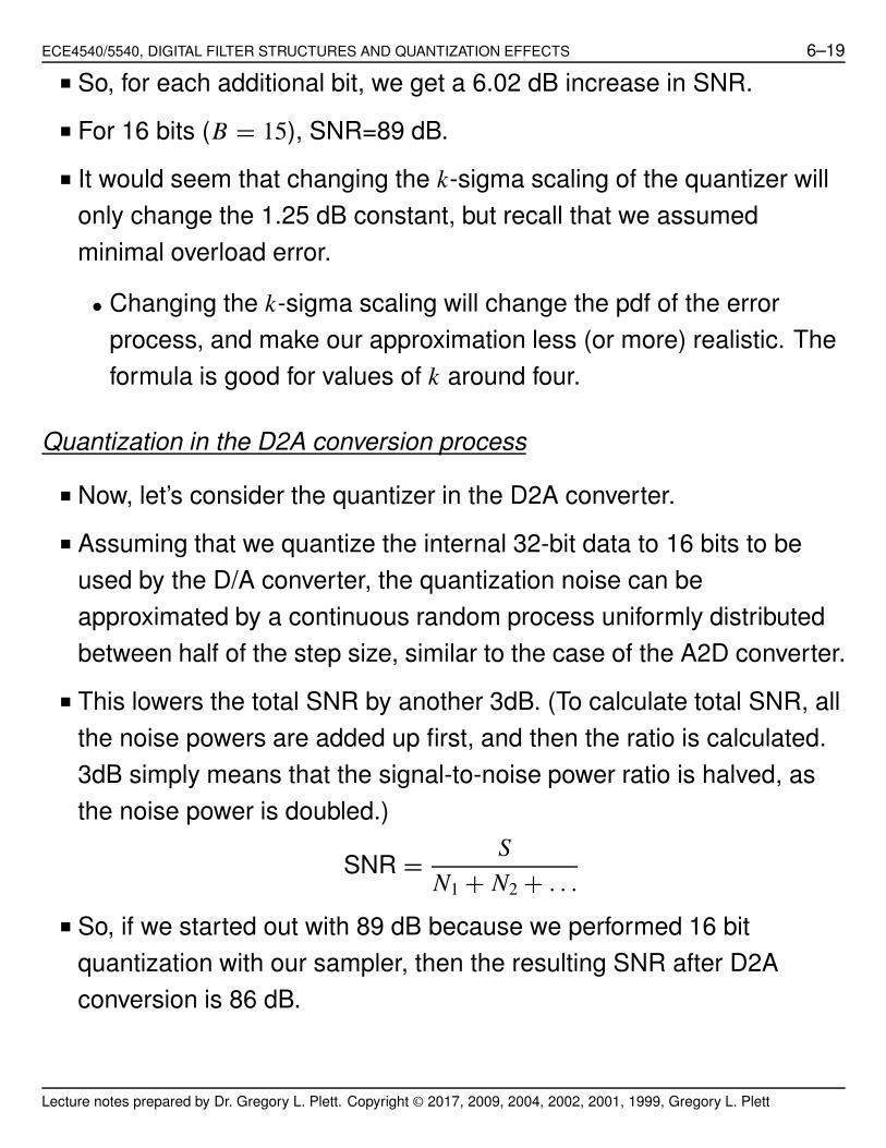
■ So, for each additional bit, we get a 6.02 dB increase in SNR.
■ For 16 bits (B = 15), SNR=89 dB.
■ It would seem that changing the k-sigma scaling of the quantizer will
only change the 1.25 dB constant, but recall that we assumed
minimal overload error.
• Changing the k-sigma scaling will change the pdf of the error
process, and make our approximation less (or more) realistic. The
formula is good for values of k around four.
Quantization in the D2A conversion process
■ Now, let’s consider the quantizer in the D2A converter.
■ Assuming that we quantize the internal 32-bit data to 16 bits to be
used by the D/A converter, the quantization noise can be
approximated by a continuous random process uniformly distributed
between half of the step size, similar to the case of the A2D converter.
■ This lowers the total SNR by another 3dB. (To calculate total SNR, all
the noise powers are added up first, and then the ratio is calculated.
3dB simply means that the signal-to-noise power ratio is halved, as
the noise power is doubled.)
SNR =S
N1 + N2 + . . .
■ So, if we started out with 89 dB because we performed 16 bit
quantization with our sampler, then the resulting SNR after D2A
conversion is 86 dB.
Lecture notes prepared by Dr. Gregory L. Plett. Copyright © 2017, 2009, 2004, 2002, 2001, 1999, Gregory L. Plett

ECE4540/5540, DIGITAL FILTER STRUCTURES AND QUANTIZATION EFFECTS 6–20
6.6: DSP-calculation signal quantization effects
■ The second quantization noise source, introduced by rounding and
truncation inside a DSP, is more complicated.
■ First, let’s take any two numbers, a and b, of 16 bits each.
■ If we multiply them together, ab will need at most 31 bits to represent
the result without losing precision.
■ Let’s look at quantization noise in IIR filters:
31
16
16 16
16
x[n] y[n]+
z−1
Q
■ IIR filters cannot be implemented with perfect precision.
• A quantizer must be placed at the output of a multiplier to limit the
number of bits in a recursive calculation.
• We need to quantify this quantization noise in order to determine
the number of bits needed to satisfy a given SNR.
■ FIR filters, on the other hand, can be implemented without
quantization noise, if the number of bits increases with the filter order.
• We seldom do this, however as the A2D and D2A converters have
already introduced some quantization noise.
• There is no point to enforce perfect precision inside a DSP when a
non-zero noise power already exists.
Lecture notes prepared by Dr. Gregory L. Plett. Copyright © 2017, 2009, 2004, 2002, 2001, 1999, Gregory L. Plett

ECE4540/5540, DIGITAL FILTER STRUCTURES AND QUANTIZATION EFFECTS 6–21
16
31
16
3116
31
16
31
16
31
16
31
16
31
x[n]
y[n]+++++
z−1 z−1 z−1 z−1
■ There are two effects to be considered when we design a quantizer
for multipliers and accumulators:
1. Quantizer step size should be kept as small as possible because
of the square term in quantization noise power, $2/12.
2. Xm should be large enough to prevent overflow.
■ Of course, these two effects contradict each other and represent a
design trade-off.
EXAMPLE: Consider the following second-order section:
x[n] y[n]++
++
z−1z−1
z−1 z−1
QUESTION: How many quantization noise sources are there in the filter?
ANSWER: It depends on where the quantizers are placed. We can have
either 1 or 5.
Lecture notes prepared by Dr. Gregory L. Plett. Copyright © 2017, 2009, 2004, 2002, 2001, 1999, Gregory L. Plett

ECE4540/5540, DIGITAL FILTER STRUCTURES AND QUANTIZATION EFFECTS 6–22
■ Assuming we have M noise sources, then the total noise power will
be M × $2/12.
■ To calculate the noise power after filtering, we need to borrow some
math from random processes.
• The Fourier transform of a random process doesn’t exist, but the
Fourier transform of the autocorrelation function of a stationary
random process does exist, called the power spectrum density.
• The power spectrum density at the output of a filter is the
multiplication of the power spectrum density of the input and the
square of the filter frequency response, as shown in the following
figure:
(tempor
x[n] y[n]
PX(e jω) PY (e jω) = PX(e jω)|H(e jω)|2H(e jω)
■ The noise power at the output of a filter is the integration of its power
spectrum density:
σ 2f = σ 2
e ×1
2π
- π
−π
..H(e jω)..2 dω
where we have assumed that the input noise power spectrum density
is a constant variance σ 2e (a white random process with zero mean).
■ By Parseval’s Theorem,
1
2π
- π
−π
..H(e jω)..2 dω =
∞!
n=−∞
|h[n]|2
so: σ 2f = σ 2
e
∞!
n=−∞
|h[n]|2.
Lecture notes prepared by Dr. Gregory L. Plett. Copyright © 2017, 2009, 2004, 2002, 2001, 1999, Gregory L. Plett

ECE4540/5540, DIGITAL FILTER STRUCTURES AND QUANTIZATION EFFECTS 6–23
■ The output noise power can be calculated by either equation, as an
integral of the power spectrum density over all frequencies, or as a
scaled infinite summation of the impulse response squared.
■ Usually it is easier to calculate the infinite summation if the impulse
response takes on a closed form.
EXAMPLE: Consider the following filter:
x[n] y[n]w[n]+
z−1
a
b
■ We first find the transfer function from w[n] to y[n]
y[n] = w[n] + ay[n − 1]
Y (z)(1 − az−1) = W (z)
Hyw(z) =Y (z)
W (z)=
1
1 − az−1=
z
z − a.
■ We next find the impulse response from w[n] to y[n]
hyw[n] = an1[n].
■ Next, the infinite summation of the squared absolute value of the
impulse response∞!
n=−∞
|an1[n]|2 =
∞!
n=0
|a2|n =1
1 − a2.
■ The noise power at the filter output is:
Lecture notes prepared by Dr. Gregory L. Plett. Copyright © 2017, 2009, 2004, 2002, 2001, 1999, Gregory L. Plett

ECE4540/5540, DIGITAL FILTER STRUCTURES AND QUANTIZATION EFFECTS 6–24
256782
sources
×X2
m2−2B
125 67 8σ 2
e
×1
1 − a25 67 8"|h[n]|2
EXAMPLE: Consider the following filter:x[n] y[n]w[n]
+
+ +
+
z−1
z−1
■ The noise power at the filter output is:
2 ×X2
m2−2B
12
∞!
n=−∞
|hyx[n]|2 + 3 ×X2
m2−2B
12
■ To calculate the signal power, we use the same concept of power
spectrum density since the input signal is merely another random
process.
■ The signal power at the output of a filter is usually expressed as:
σ 2s = σ 2
input
∞!
n=−∞
|h[n]|2
where σ 2input is the input signal power. [Input assumed “white” too!]
■ The total SNR is the ratio of the signal power to the noise power.
Lecture notes prepared by Dr. Gregory L. Plett. Copyright © 2017, 2009, 2004, 2002, 2001, 1999, Gregory L. Plett

ECE4540/5540, DIGITAL FILTER STRUCTURES AND QUANTIZATION EFFECTS 6–25
6.7: Dynamic range scaling: Criteria
■ Overflow occurs when two numbers are added and the result requires
more than B + 1 bits to store.
EXAMPLE: For four-bit quantization:
0.111 positive number (7/8)
+ 0.011 positive number (3/8)
1.010 negative number (−6/8)
■ In this overflow situation we can either “clip” the result or leave it as is.
■ To clip the result, replace a positive result with 0.1111. . . ; a negative
result with 1.00000. . . .
■ The input/output relationship of a
clipping (saturating) quantizer is:
■ We would like to ensure that
saturation does not occur.
Scaling criterion #1: Bounded-input-bounded output.
■ In this criterion we want to make sure that every node in the filter
network is bounded by some number.
■ If we follow the convention that each number represents a fraction of
unity (with a possible implied scaling factor) each node in the network
must be constrained to have a magnitude less than 1 to avoid
overflow.
■ Pick any node in the network w[n]. Its response can be expressed as:
Lecture notes prepared by Dr. Gregory L. Plett. Copyright © 2017, 2009, 2004, 2002, 2001, 1999, Gregory L. Plett
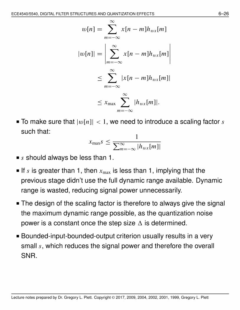
ECE4540/5540, DIGITAL FILTER STRUCTURES AND QUANTIZATION EFFECTS 6–26
w[n] =
∞!
m=−∞
x[n − m]hwx[m]
|w[n]| =
.....
∞!
m=−∞
x[n − m]hwx[m]
.....
≤
∞!
m=−∞
|x[n − m]hwx[m]|
≤ xmax
∞!
m=−∞
|hwx[m]|.
■ To make sure that |w[n]| < 1, we need to introduce a scaling factor s
such that:
xmaxs ≤1"∞
m=−∞ |hwx[m]|
■ s should always be less than 1.
■ If s is greater than 1, then xmax is less than 1, implying that the
previous stage didn’t use the full dynamic range available. Dynamic
range is wasted, reducing signal power unnecessarily.
■ The design of the scaling factor is therefore to always give the signal
the maximum dynamic range possible, as the quantization noise
power is a constant once the step size $ is determined.
■ Bounded-input-bounded-output criterion usually results in a very
small s, which reduces the signal power and therefore the overall
SNR.
Lecture notes prepared by Dr. Gregory L. Plett. Copyright © 2017, 2009, 2004, 2002, 2001, 1999, Gregory L. Plett

ECE4540/5540, DIGITAL FILTER STRUCTURES AND QUANTIZATION EFFECTS 6–27
Scaling criterion #2: Frequency-response criterion.
■ This criterion assumes we are inputting a narrow-band signal
x[n] = xmax cos ω0n to the filter.
■ To avoid overflow at node w[n] given this input signal, we need to
ensure that
|w[n]| = |Hwx(ejω0)|xmax ≤ 1.
■ The scaling factor s should be chosen so that:
xmaxs ≤1
max0≤ω≤π |Hwx(e jω)|.
■ Because max0≤ω≤π
|Hwx(ejω)| ≤
∞!
m=−∞
|hwx[m]|, the scaling factor derived
using Criterion #1 is always smaller than the scaling factor derived
using Criterion #2.
EXAMPLE: Consider the following simple filter. Assuming that xmax = 1,
scale the input so that |y[n]| is always less than 1.
x[n] y[n]w[n]+
z−1
a
b
■ To find the scaling factor using Criterion #1, we need to calculate the
summation of the absolute values of the impulse response:
s =1"∞
m=−∞ |h[m]|=
1"∞m=0 |b||a|m
=1 − |a|
|b|.
Lecture notes prepared by Dr. Gregory L. Plett. Copyright © 2017, 2009, 2004, 2002, 2001, 1999, Gregory L. Plett

ECE4540/5540, DIGITAL FILTER STRUCTURES AND QUANTIZATION EFFECTS 6–28
EXAMPLE: Find the output SNR
■ The output noise power is simply 2 × $2/12 × 1/(1 − a2).
■ To calculate the signal power, assume that x[n] is a white random
signal uniformly distributed between 1 and −1.
• Its mean is 0 and its variance is 1/3.
• The signal power at the output of the filter is1
3s2 b2
1 − a2.
■ The total SNR is:
1
3s2 b2
1 − a2×
12(1 − a2)
2$2=
2s2b2
$2=
2(1 − |a|)2
$2.
Lecture notes prepared by Dr. Gregory L. Plett. Copyright © 2017, 2009, 2004, 2002, 2001, 1999, Gregory L. Plett
ECE4540/5540, DIGITAL FILTER STRUCTURES AND QUANTIZATION EFFECTS 6–29
6.8: Dynamic range scaling: Application
Scaling for parallel and cascade structures
■ Scaling strategy for cascade or parallel second-order IIR filters is a
trade-off between avoiding overflow and reducing
signal-to-quantization noise of the overall system.
■ For cascade IIR filters, let’s take a look at the following example, a
three-stage lowpass filter:
H(z) = b0
3%
k=1
(1 + b1kz−1 + b2kz−2)
(1 − a1kz−1 − a2kz−2).
■ Because there is a small gain constant b0, the three cascade stages
actually produce high gain at some internal nodes to produce an
overall gain of unity at dc.
• If we put the gain constant at the input to the filter, the signal
power is reduced immediately, while the noise power is to be
amplified by the rest of the system.
• On the other hand, if we put the gain constant at the end of the
filter, we will have overflow along the cascade because of the high
gain introduced internally by the three stages.
■ The scaling strategy is to distribute the gain constant along the three
stages so that overflow is just avoided at each stage of the cascade.
Lecture notes prepared by Dr. Gregory L. Plett. Copyright © 2017, 2009, 2004, 2002, 2001, 1999, Gregory L. Plett
ECE4540/5540, DIGITAL FILTER STRUCTURES AND QUANTIZATION EFFECTS 6–30
EXAMPLE: H(z) = s1H1(z)s2H2(z)s3H3(z).x[n] y[n]w1[n] w2[n] w3[n]s1
s2 s3
+ +
+++
++++
+ + +
z−1
z−1
z−1z−1
z−1 z−1
■ Noise power,
Pf (ω) =2−2B
12
/3s2
2|H2(ejω)|2s2
3|H3(ejω)|2
|A1(e jω)|2+
5s23|H3(e
jω)|2
|A2(e jω)|2
+5
|A3(e jω)|2+ 3
0
■ Note: 1/Ak(ejω) is the transfer function of the feedback from wk[n] to
the output of that filter stage.
■ To maximize the total SNR is not a trivial task. Let’s first make sure
that no overflow can happen at all nodes. Using our Criterion #2:
• Scaling s1 according to s1 maxω
|H1(ejω)| < 1,
• Scaling s2 according to s1s2 maxω
|H1(ejω)H2(e
jω)| < 1,
• Scaling s3 according to s1s2s3 = b0.
QUESTION: How do we pair poles and zeros in H1, H2, and H3 to make
our stages?
Pole-zero pairing in cascade IIR filters
■ There are N ! ways to pair zeros and poles if there are N cascade
stages, which is obviously a very computationally intensive problem.
Lecture notes prepared by Dr. Gregory L. Plett. Copyright © 2017, 2009, 2004, 2002, 2001, 1999, Gregory L. Plett

ECE4540/5540, DIGITAL FILTER STRUCTURES AND QUANTIZATION EFFECTS 6–31
■ Optimal solutions can be found through dynamic programming, but a
very good heuristic algorithm proposed by Jackson is usually used.1
1. The pole that is closest to the unit circle should be paired with the
zero that is closest to it in the z-plane.
2. Step 1 should be repeatedly applied until all the poles and zeros
have been paired.
■ The intuition behind Step 1 is based on the observation that a
second-order section with high gain (its poles close to the unit circle)
is undesirable because it can cause overflow and amplify quantization
noise.
■ Pairing a pole that is close to the unit circle with an adjacent zero
tends to reduce the peak gain of the section, equalizing the gain
along the cascade stages.
1 Leland Jackson, Digital Filters and Signal Processing, 3d, Kluwer Academic Publish-ers, 1996.
Lecture notes prepared by Dr. Gregory L. Plett. Copyright © 2017, 2009, 2004, 2002, 2001, 1999, Gregory L. Plett

ECE4540/5540, DIGITAL FILTER STRUCTURES AND QUANTIZATION EFFECTS 6–32
Cascade stage ordering
■ Jackson’s advice isn’t as useful here: “Second-order sections should
be ordered according to the closeness of the poles to the unit circle,
either in order of increasing closeness to the unit circle or in order of
decreasing closeness to the unit circle.”
■ The reason for the uncertainty is this:
• A highly peaked filter section (poles close to the unit circle) should
be put toward the beginning of the cascade so that its transfer
function doesn’t occur often in the noise power equation.
• On the other hand, a highly peaked section should be placed
toward the end of the cascade to avoid excessive reduction of the
signal level in the early stages of the cascade (small s values at
the beginning of a cascade attenuate signal power but not
quantization noise power).
• Therefore without extensive simulation, the best we can have is a
set of “rules of thumb”, one of which is stated as above.
■ Parallel IIR filters are a bit easier to deal with, because the issue of
pairing and ordering does not arise.
• Jackson concluded that the total signal-to-quantization noise of the
parallel form is comparable to that of the best pairing and ordering
of the cascade form.
• But cascade form is more commonly used because of its control
over zeros as we discussed in coefficient quantization.
Lecture notes prepared by Dr. Gregory L. Plett. Copyright © 2017, 2009, 2004, 2002, 2001, 1999, Gregory L. Plett

ECE4540/5540, DIGITAL FILTER STRUCTURES AND QUANTIZATION EFFECTS 6–33
6.9: Zero-input limit cycles
■ The term “zero-input limit cycle” refers to the phenomenon where a
system’s output continues to oscillate indefinitely while the input
remains equal to zero, caused by the nonlinear characteristic of a
quantizer in the feedback loop of the system.
■ We will consider the limit-cycle effects for only first-order and
second-order filters.
EXAMPLE: Consider the filter y[n] = ay[n − 1] + x[n].
(system
x[n] y[n]+
z−1
a
■ Limit cycles appear when the system behaves as if there is a pole on
the unit circle. How could this happen?
■ Let’s take a closer look at quantizing ay[n − 1].
|Q(ay[n − 1]) − ay[n − 1]| ≤1
2(2−B).
■ Therefore,
|Q(ay[n − 1])| − |ay[n − 1]| ≤1
2(2−B).
■ If |Q(ay[n − 1])| = |y[n − 1]|, this implies
|y[n − 1]| − |ay[n − 1]| ≤1
2(2−B).
■ In other words, we can define a deadband of:
|y[n − 1]| ≤12(2−B)
1 − |a|.
Lecture notes prepared by Dr. Gregory L. Plett. Copyright © 2017, 2009, 2004, 2002, 2001, 1999, Gregory L. Plett

ECE4540/5540, DIGITAL FILTER STRUCTURES AND QUANTIZATION EFFECTS 6–34
■ Whenever y[n] falls within this deadband when the input is zero, the
filter remains in the limit cycle until an input is applied.
EXAMPLE: Suppose that we use a 4-bit quantizer to implement a
first-order filter of a = 1/2.
■ We calculate the deadband size to be12(2−3)
1 − 12
= 2−3 =1
8.
■ If the initial condition y[−1] is equal to 7/8, or 0.111, then:
ay[−1] = y[0] = 0.0111 → 0.100
ay[0] = y[1] = 0.0100 → 0.010
ay[1] = y[2] = 0.0010 → 0.001
ay[2] = y[3] = 0.0001 → 0.001
ay[3] = y[4] = 0.0001 → 0.001
QUESTION: What if a = −1/2?
ANSWER: The output will oscillate between 1/8 and −1/8.
■ For second-order sections, the analysis is a bit more complicated:
y[n] = x[n] + Q(a1y[n − 1]) + Q(a2y[n − 2]).
■ Recall that a1 corresponds to 2r cos θ and a2 corresponds to r2.
■ We concentrate on the a2 term, as it defines the distance of the two
complex-conjugate poles to the origin.
■ If we have:
Q(a2y[n −2]) = −y[n −2] and |Q(a2y[n −2])−a2y[n −2]| ≤1
2(2−B)
then |y[n − 2]| ≤12(2−B)
|1 + a2|, the deadband for a second-order filter.
Lecture notes prepared by Dr. Gregory L. Plett. Copyright © 2017, 2009, 2004, 2002, 2001, 1999, Gregory L. Plett

ECE4540/5540, DIGITAL FILTER STRUCTURES AND QUANTIZATION EFFECTS 6–35
■ When the input is zero and the output falls within this range, the
effective value of a2 is such that the poles are on the unit circle.
QUESTION: What does a1 do?
ANSWER: a1 controls the oscillation frequency.
EXAMPLE: y[n] = Q(1/2y[n − 1]) + Q(−7/8y[n − 2]) with a four-bit
quantizer.
■ The deadband is equal to 2−3 ×1
2× 8 =
1
2.
■ If the initial condition is such that y[−1] = y[−2] = 1/8, the output will
oscillate between 0, −1/8, −1/8, 0, 1/8, 1/8, etc.
■ Adding dither to the input signal can sometimes be effective in
eliminating limit cycles. See Franklin.
Where to from here?
■ We have now completed the fundamental material of this course.
■ We can analyze and design hybrid control systems using traditional
means.
■ We have seen that some less common methods, such as direct
coefficient optimization and Ragazzini’s method, can improve on
simple lead/lag (and so forth) designs.
■ How far can we take this idea? Can we adaptively optimize
control-system design?
■ That’s the topic we look at last in this course.
Lecture notes prepared by Dr. Gregory L. Plett. Copyright © 2017, 2009, 2004, 2002, 2001, 1999, Gregory L. Plett