Digital Image Processing (CS/ECE 545) Lecture 9: Color Images (Part 2) & 

Introduction to Spectral Techniques (Fourier Transform, DFT, DCT)

Prof Emmanuel Agu

Computer Science Dept.Worcester Polytechnic Institute (WPI)

Organization of Color Images

True color: Uses all colors in color space Indexed color: Uses only some colors  Which subset of colors to use? Depends on application

True color:  used in applications that contain many colors with subtle 

differences  E.g. digital photography or photorealistic rendering

Two main ways to organize true color  Component ordering Packed ordering

True Color: Component Ordering

Colors in 3 separate arrays of similar length Retrieve same location (u,v) in each R, G and B array

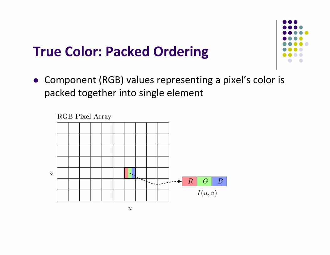
True Color: Packed Ordering

Component (RGB) values representing a pixel’s color is packed together into single element

Indexed Images Permit only limited number of distinct colors (N = 2 to 256) Used in illustrations or graphics containing large regions with 

same color Instead of intensity values, image contains indices into color 

table or palette Palette saved as part of image Converting from true color to indexed color requires 

quantization

Color Images in ImageJ

ImageJ supports 2 types of color images RGB full‐color images (24‐bit “RGB color”), 

packed order Supports TIFF, BMP, JPEG, PNG and RAW file formats

Indexed images (“8‐bit color”) Up to 256 colors max (8 bits) Supports GIF, PNG, BMP and TIFF (uncompressed) file formats

See section 12.1.2 of Burger & Burge

Color Image Conversion in ImageJ

Methods for converting between different types of color and grayscale image objects

Note: if doScaling is true, pixel values scaled to maximum range of new image

Conversion to ImagePlus Objects

Do not create new image. Just modify original ImagePlus object

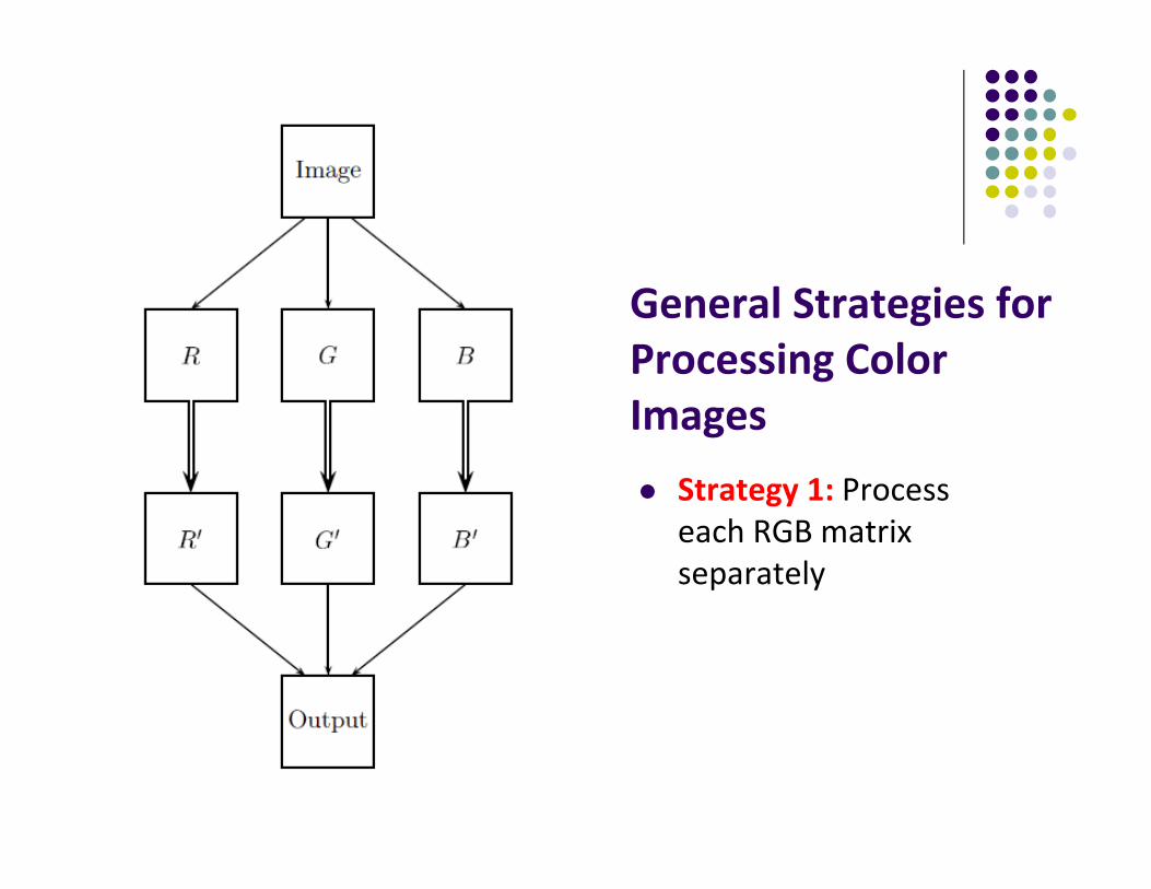
General Strategies for Processing Color Images Strategy 1: Process 

each RGB matrix separately

General Strategies for Processing Color Images Strategy 2: Compute 

luminance (weighted average of RGB), process intensity matrix 

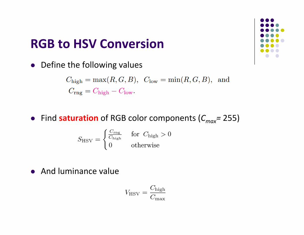
RGB to HSV Conversion Define the following values

Find saturation of RGB color components (Cmax= 255)

And luminance value

RGB to HSV Conversion

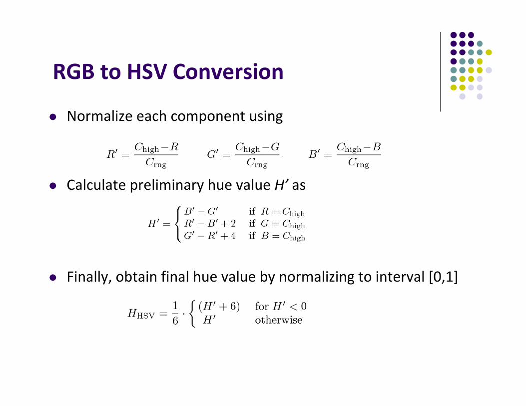
Normalize each component using

Calculate preliminary hue value H’ as 

Finally, obtain final hue value by normalizing to interval [0,1]

Example: RGB to HSV Conversion

Original RGB image

HSV values in grayscale

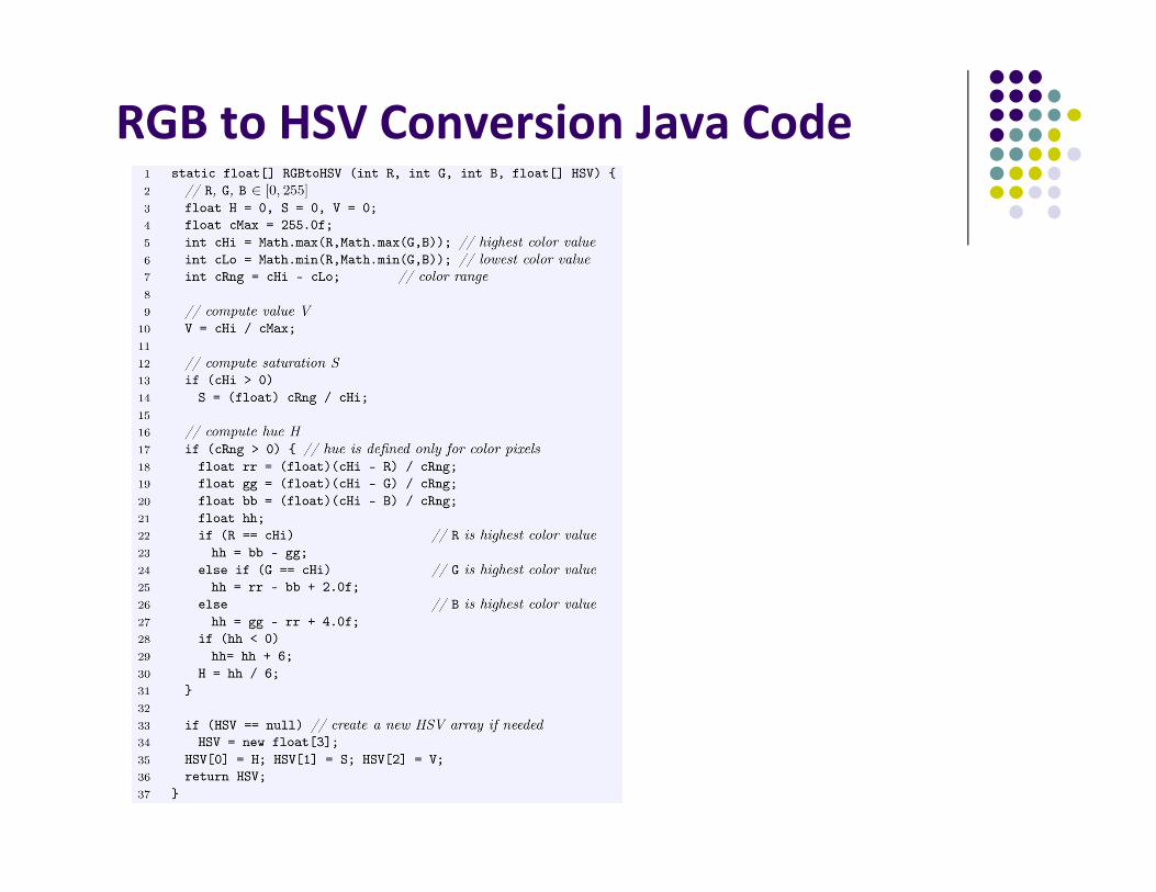
RGB to HSV Conversion Java Code

HSV to RGB Conversion

HSV to RGB Conversion

RGB Components can be scaled to whole numbers in range [0,255] as

HSV to RGB Code

RGB to HLS Conversion

Compute Hue same way as for HSV model

Then compute the other 2 values as:

Example RGB to HLS Conversion

Original RGB image

HLS values in grayscale

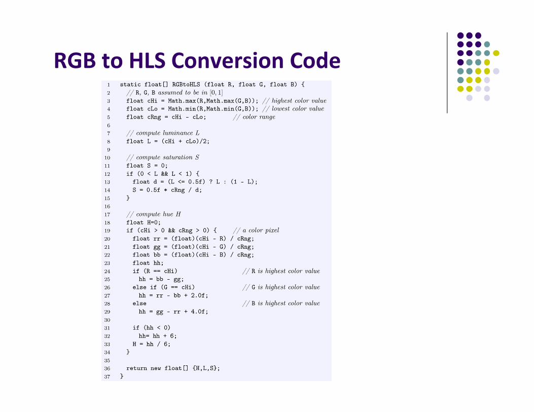
RGB to HLS Conversion Code

HLS to RGB Conversion Assuming H, L and S in [0,1] range

Otherwise, calculate

Then calculate the values

HLS to RGB Conversion

Assignment of RGB values is done as follows

HLS to RGB Code

TV Color Spaces – YUV, YIQ, YCbCr YUV, YIQ: color encoding for analog NTSC and PAL YCbCr: Digital TV encoding Key common ideas: Separate luminance component Y from 2 chroma 

components Instead of encoding colors, encode color differences 

between components (maintains compatibility with black and white TV)

YUV

Basis for color encoding in analog TV in north america (NTSC) and Europe (PAL)

Y components computed from RGB components as

UV components computed as:

YUV

Entire transformation from RGB to YUV

Invert matrix above to transform from YUV back to RGB

YIQ

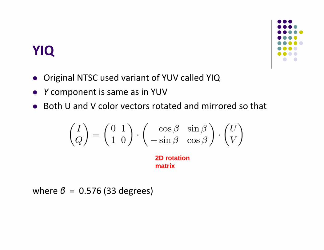
Original NTSC used variant of YUV called YIQ Y component is same as in YUV Both U and V color vectors rotated and mirrored so that

where β =  0.576 (33 degrees)

2D rotation matrix

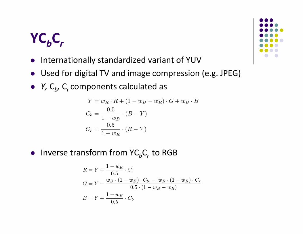
YCbCr Internationally standardized variant of YUV Used for digital TV and image compression (e.g. JPEG) Y, Cb, Cr components calculated as 

Inverse transform from YCbCr  to RGB

YCbCr ITU recommendation BT.601 specifies values:

wR = 0.299,    wB = 0.114,     wG = 1 – wB – wR = 0.587 Thus the transformation

And the inverse transformation becomes

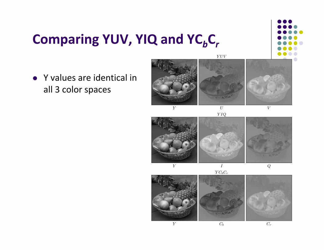
Comparing YUV, YIQ and YCbCr

Y values are identical in all 3 color spaces

CIE Color Space

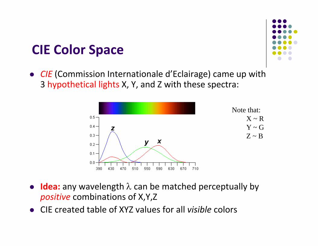
CIE (Commission Internationale d’Eclairage) came up with 3 hypothetical lights X, Y, and Z with these spectra:

Idea: any wavelength  can be matched perceptually by positive combinations of X,Y,Z

CIE created table of XYZ values for all visible colors

Note that:X ~ RY ~ GZ ~ B

CIE Color Space

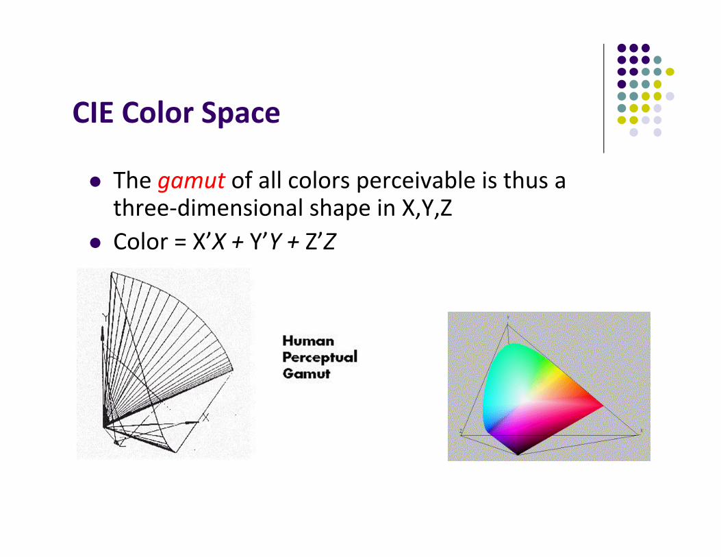
The gamut of all colors perceivable is thus a three‐dimensional shape in X,Y,Z

Color = X’X + Y’Y + Z’Z

CIE Chromaticity Diagram (1931)

•For simplicity, we often project to the 2D plane •Also normalize

•Note: Inside horseshoe visible, outside invisible to eye

Note: Look up x, yCalculate z as 1 – x - y

Standard Illuminants

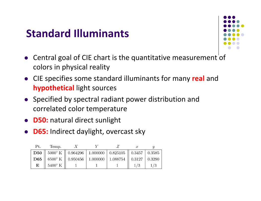
Central goal of CIE chart is the quantitative measurement of colors in physical reality

CIE specifies some standard illuminants for many real and hypothetical light sources 

Specified by spectral radiant power distribution and correlated color temperature

D50: natural direct sunlight D65: Indirect daylight, overcast sky

CIE uses Find complementary colors:  equal linear distances from white in opposite directions

Measure hue and saturation:  Extend line from color to white till it cuts horseshoe (hue) Saturation is ratio of distances color‐to‐white/hue‐to‐white 

Define and compare device color gamut (color ranges) Problem: not perceptually uniform:  Same amount of changes in different directions generate 

perceived difference that are not equal CIE LUV, L*a*b* ‐ uniform

CIE L*a*b*

Main goal was to make changes in this space linear with respect to human perception

Now popular in high‐quality photographic applications Used in Adobe photoshop as standard for converting between 

different color spaces Components:

Luminosity L  Color components a* and b* which specify color hue and saturation 

along green‐red and blue‐yellow axes

All 3 components are measured relative to reference white Non‐linear correction function (like gamma correction) applied

Device Color Gamuts

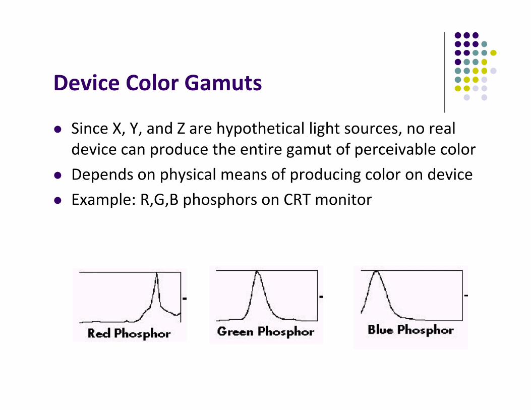
Since X, Y, and Z are hypothetical light sources, no real device can produce the entire gamut of perceivable color

Depends on physical means of producing color on device Example: R,G,B phosphors on CRT monitor

Device Color Gamuts

The RGB color cube sits within CIE color space We can use the CIE chromaticity diagram to compare the 

gamuts of various devices  E.g. compare color printer and monitor color gamuts

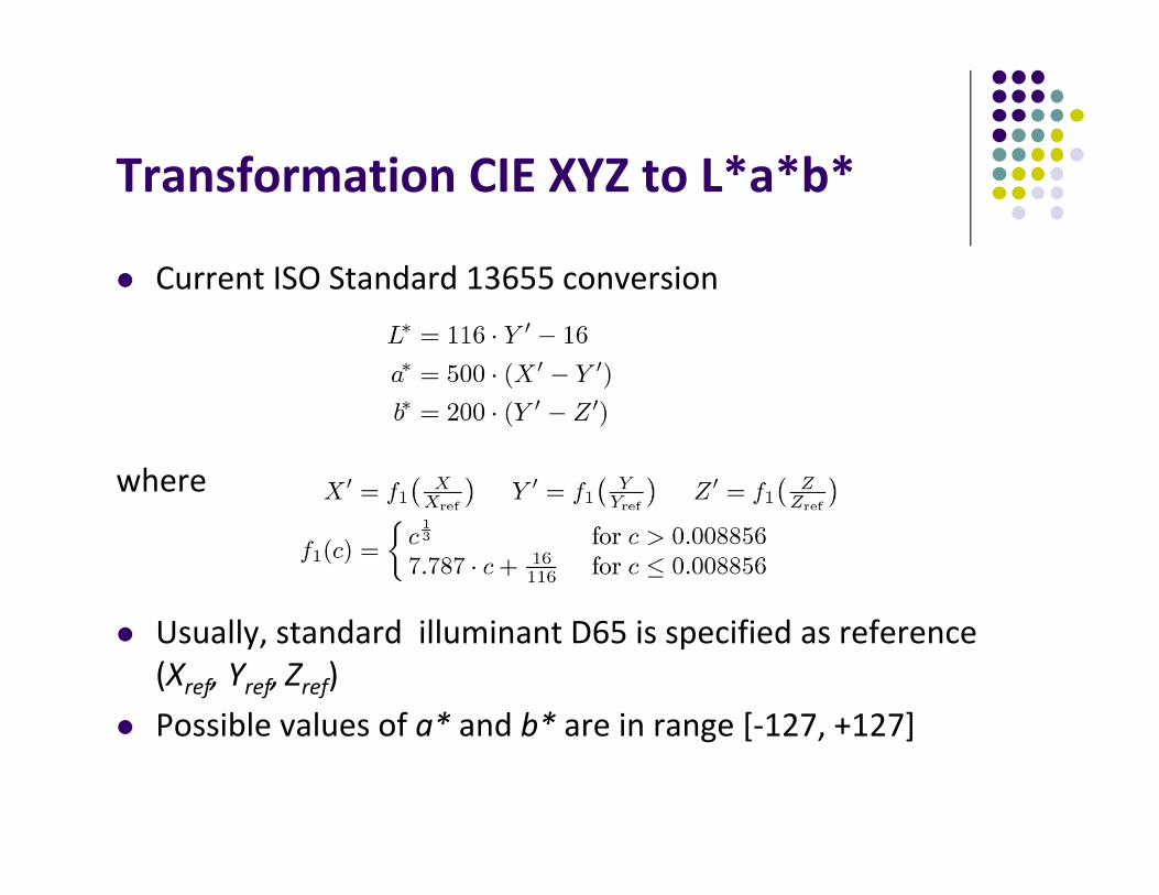
Transformation CIE XYZ to L*a*b*

Current ISO Standard 13655 conversion

where

Usually, standard  illuminant D65 is specified as reference (Xref, Yref, Zref)

Possible values of a* and b* are in range [‐127, +127]

Transformation L*a*b* to CIE XYZ

Reverse transformation from L*a*b* space to XYZ is

where

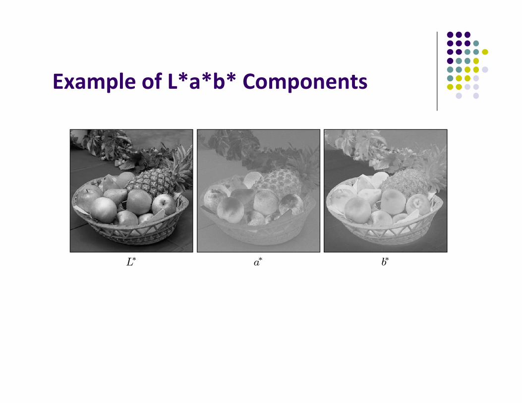
Example of L*a*b* Components

Code for XYZ to L*a*b* and L*a*b* to XYZ Conversion

Measuring Color Differences

Due to its uniformity with respect to human perception, differences between colors in L*a*b* color space can be determined as euclidean distance

sRGB

For many computer display‐oriented applications, use of CIE color space may be too cumbersome

sRGB  developed by Hewlett Packard and Microsoft has relatively small gamut compared to L*a*b*  Its colors can be reproduced by most computer monitors De Facto standard for digital cameras

Several image formats (EXIF, PNG) based on sRGB

Transformation CIE XYZ to sRGB

First compute linear RGB values as

Where

Next gamma correct linear RGB values

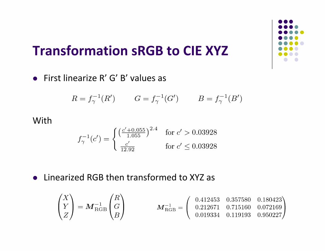
Transformation sRGB to CIE XYZ

First linearize R’ G’ B’ values as

With

Linearized RGB then transformed to XYZ as

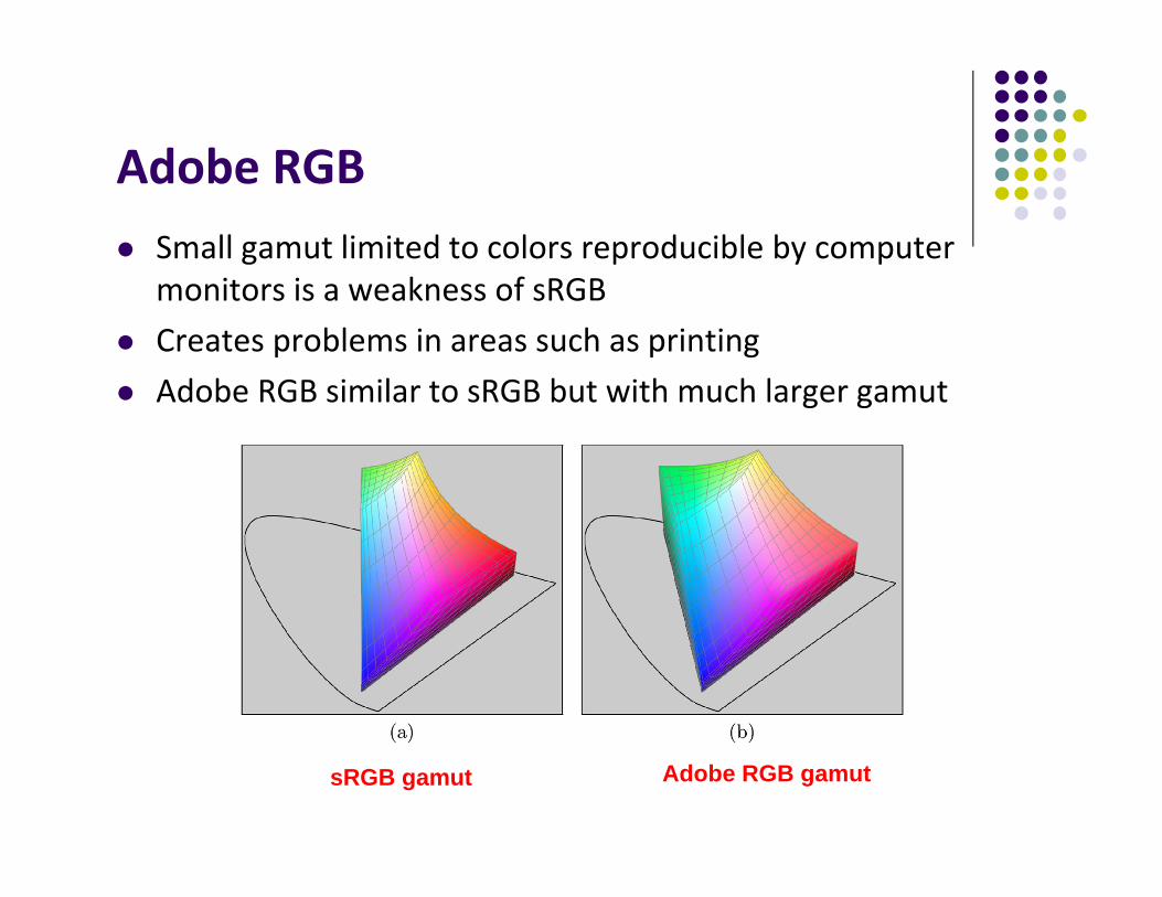
Adobe RGB Small gamut limited to colors reproducible by computer 

monitors is a weakness of sRGB Creates problems in areas such as printing Adobe RGB similar to sRGB but with much larger gamut

sRGB gamut Adobe RGB gamut

Chromatic Adaptation

Human eye adapts to make color of object same under different lighting conditions

E.g. Paper appears white in bright daylight and under flourescent light

CIE color system allows colors to be specified relative to white point, called relative colorimetry

If 2 colors specified relative to different white points, they can be related to each other using chromatic adaptation transformation (CAT)

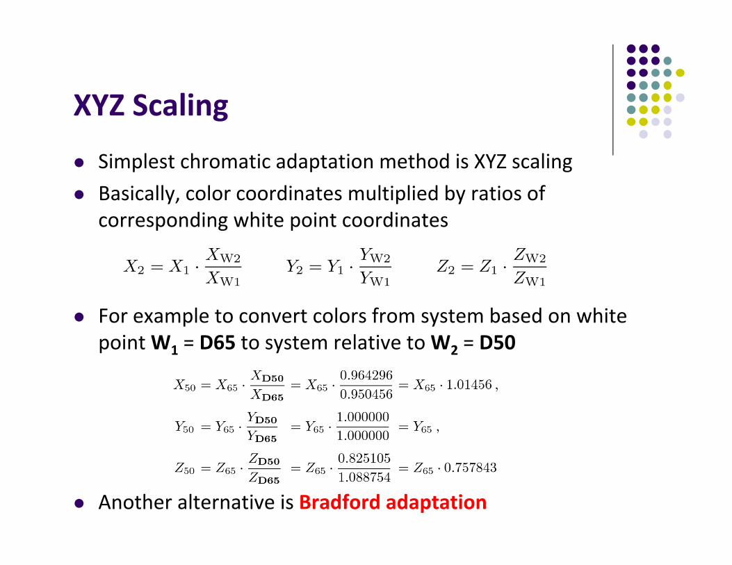
XYZ Scaling

Simplest chromatic adaptation method is XYZ scaling Basically, color coordinates multiplied by ratios of 

corresponding white point coordinates

For example to convert colors from system based on white point W1 = D65 to system relative to W2 = D50

Another alternative is Bradford adaptation

Colorimetric Support in Java

sRGB is standard color space in Java  Components of color objects and RGB color images are color 

corrected

Statistics of Color Images

Task: Determine how many unique colors in a given image Approach 1: Create histogram, count frequency of each color

Not efficient since for 24‐bit image, there are 224 = 16,777,216 colors

Approach 2: Put pixels in array, then sort Similar colors next to each other We can then count the number of transitions between neighboring 

colors Much more efficient than histogram approach if many repeated colors

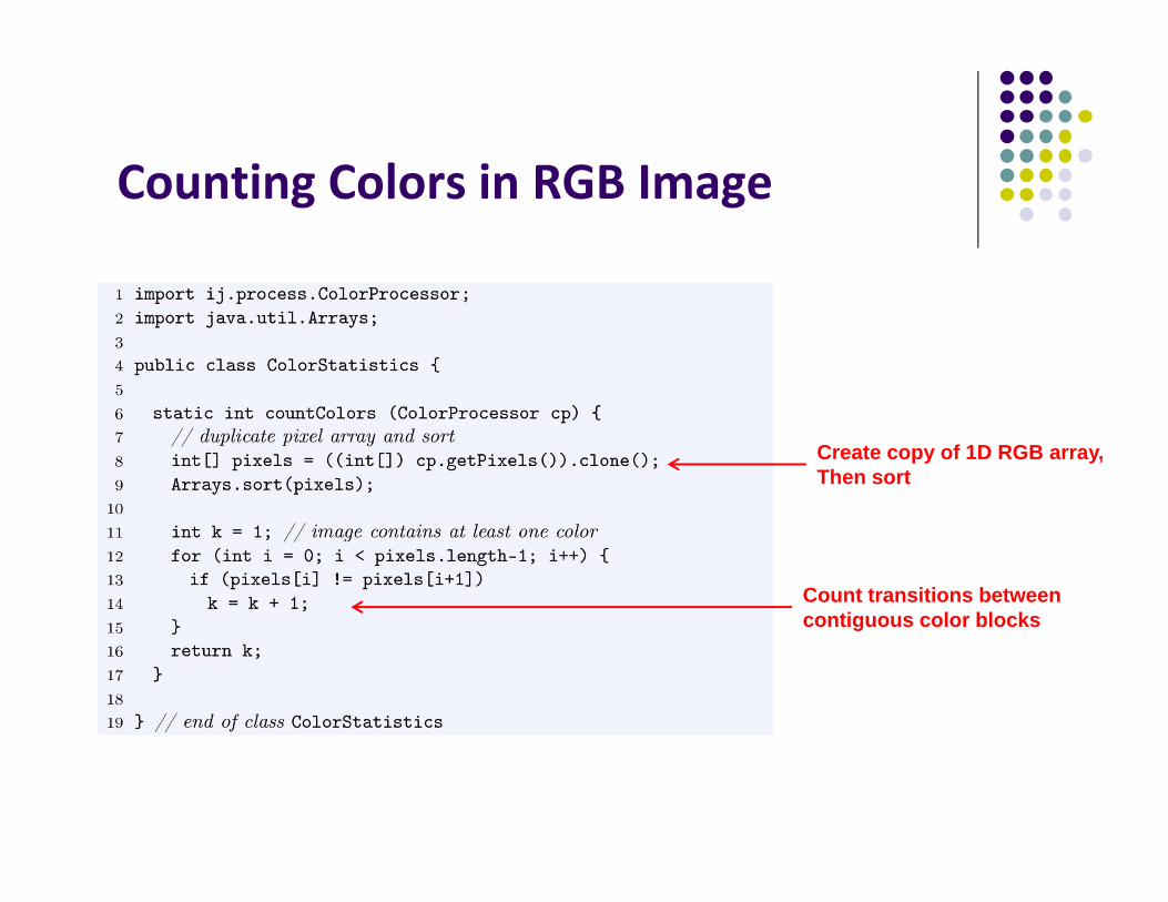
Counting Colors in RGB Image

Create copy of 1D RGB array,Then sort

Count transitions between contiguous color blocks

Color Histograms

When applied to object of type ColorProcessor, built‐in ImageJ method getHistogram( ), simply counts intensity of corresponding gray values

Another alternative: compute individual intensity histograms of 3 color channels Downside: does not give information about actual colors in image

A good alternative: 2D color histograms

2D Color Histograms Define:

Note: * denotes arbitrary component value  Resulting 2D histograms are independent of original image 

size, easily visualized

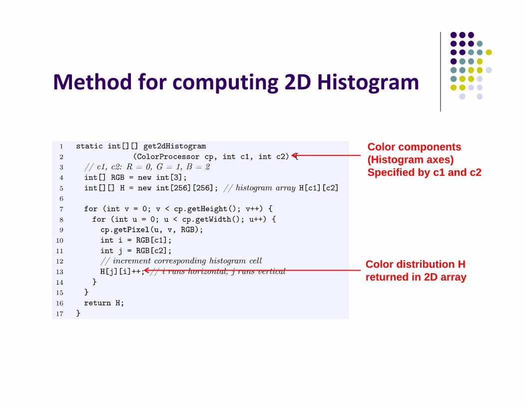
Method for computing 2D Histogram

Color components(Histogram axes) Specified by c1 and c2

Color distribution Hreturned in 2D array

Example: Combined Color Histogram

Color Quantization

True color can be quite large in actual description Sometimes need to reduce size Examples: Convert 24‐bit TIFF to 8‐bit TIFF Take a true‐color description from database and convert to web 

image format

Replace true‐color with “best match” from smaller subset Quantization algorithms: Uniform quantization Popularity algorithm Median‐cut algorithm Octree algorithm

Scalar Color Quantization Convert each component of each original RGB value  

independently from range [0,…, m‐1] to [0,….n‐1]

Example: Convert color image with 3x12‐bit components (m=4096) to RGB image with 3x8‐bit components (n=256) Multiply each component in orginal color by n/m = 256/4096 = 1/16 Result is then truncated 

Sometimes m and n not same for all components E.g. 3:3:2 packing = 3 bits for red, 3 bits for green and 2 bits 

for blue

Scalar Quantization

Distribution of 226,321colors before scalar 3:3:2 quantization

Quantizationof 3x12-bit to3x8-bit colors

Quantizationof 3x8-bit to3:3:2-packed 8-bit colors

256 colors after scalar 3:3:2 quantization

Vector Quantization

Does not treat individual components separately Each color of pixel treated as single entity Goal: 

1. To find set of n representative color vectors 2. Replace each original color by one of the new color vectors

n is usually pre‐determined Resulting deviation should be minimal Turns out to be an expensive global optimization problem Following methods thus calculate local optima

Populousity algorithm Median‐cut algorithm

Populosity Algorithm

Selects n most frequently occurring colors in image as representative set of color vectors

General algorithm: Sort image colors into array, Populate histogram as before pick n most frequently occurring colors as representative set For each original color, replace with closest color in representative set

Note: closest color also shortest distance in color space

Algorithm performs well as long as colors not scattered a lot

Median‐Cut Algorithm Considered classical method for color quantization Implemented in many applications and in ImageJ Algorithm:

Compute color histogram of original image Recursively divide RGB color space till number of boxes equal to desired 

number of representative colors is reached At each step of recursion, box with most pixels is split at median of the 

longest of its 3 axes so that half pixels left in each subbox In the last step, the mean color of all pixels in each subbox is computed and 

used as the representative color (each contained pixel is replaced by this mean)

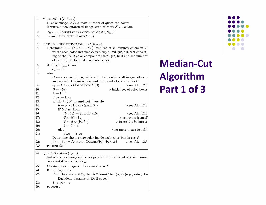
Median‐Cut AlgorithmPart 1 of 3

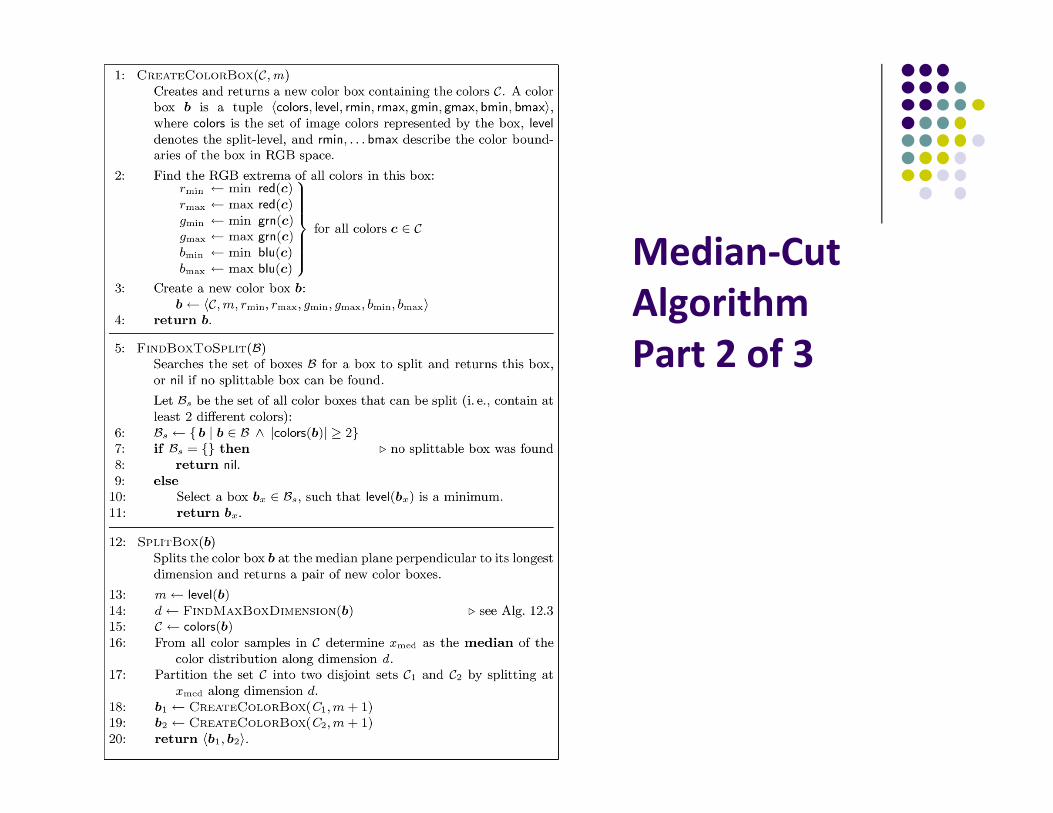
Median‐Cut AlgorithmPart 2 of 3

Median‐Cut AlgorithmPart 3 of 3

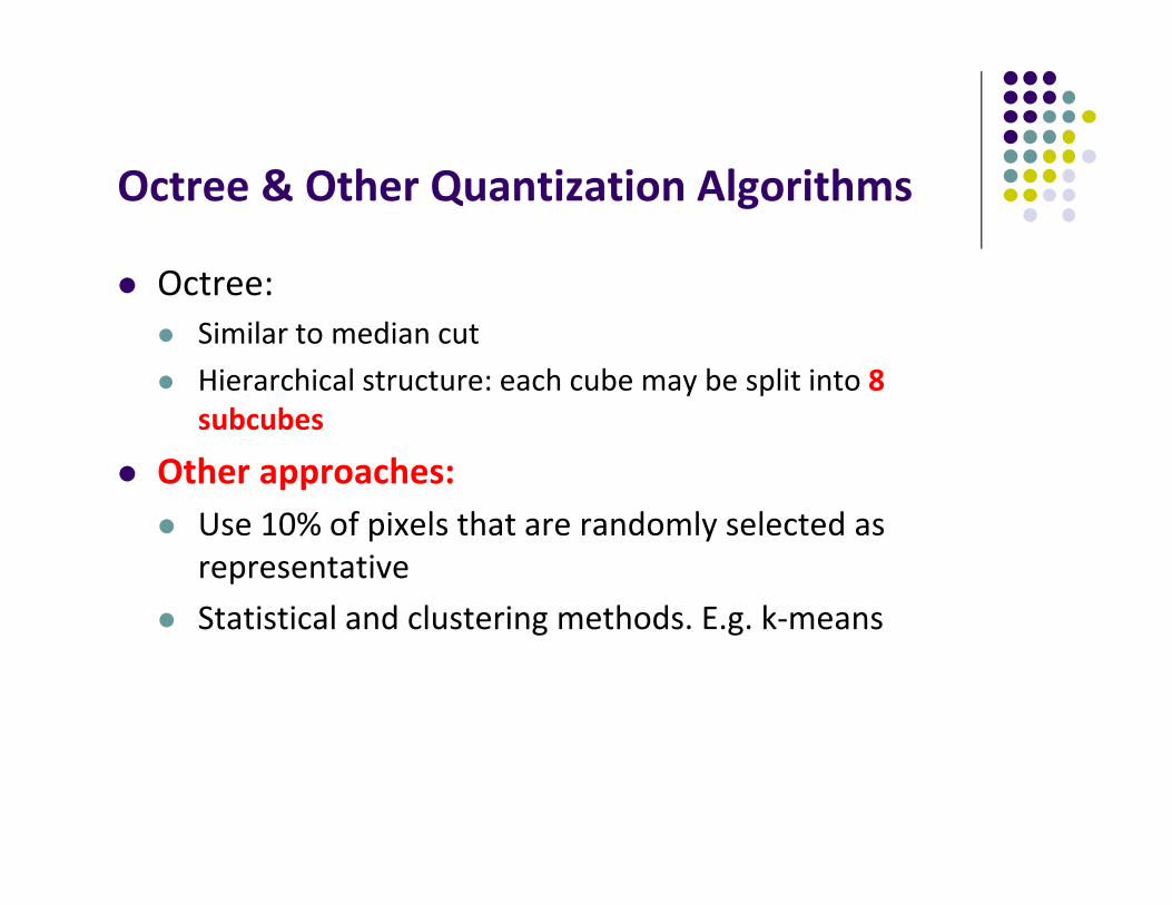
Octree & Other Quantization Algorithms

Octree: Similar to median cut Hierarchical structure: each cube may be split into 8 

subcubes

Other approaches: Use 10% of pixels that are randomly selected as 

representative Statistical and clustering methods. E.g. k‐means

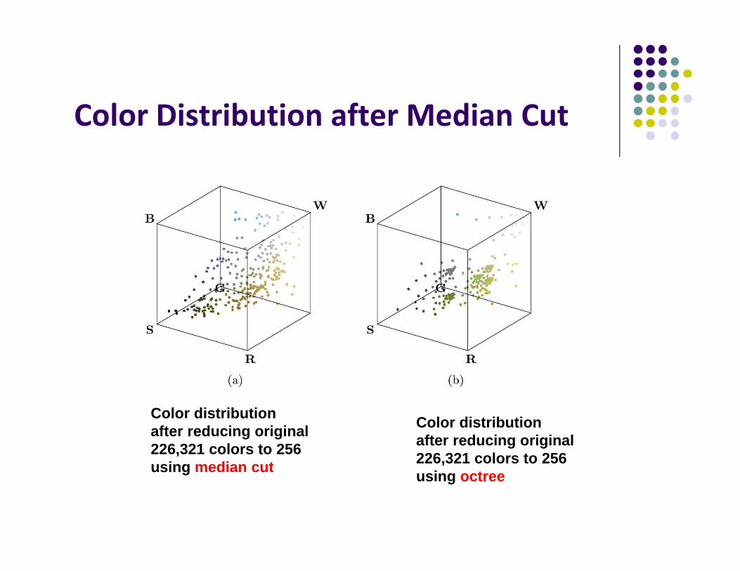
Color Distribution after Median Cut

Color distributionafter reducing original226,321 colors to 256using median cut

Color distributionafter reducing original226,321 colors to 256using octree

Comparison of Quantization Errors

OriginalImage

Octree

Distance between original and quantized colorfor scalar 3:3:2packing

Median Cut

Digital Image Processing (CS/ECE 545) Lecture 9: Color Images (Part 2) & 

Introduction to Spectral Techniques (Fourier Transform, DFT, DCT)

Prof Emmanuel Agu

Computer Science Dept.Worcester Polytechnic Institute (WPI)

Fourier Transform Main idea: Any periodic function can be decomposed into a 

summation of sines and cosines

Complex function

Sine function 1

Sine function 2

Sine function 3

Complex function expressed as sum of sines

Fourier Transform: Why? Mathematially easier to analyze effects of transmission 

medium, noise, etc on simple sine functions, then add to get effect on complex signal

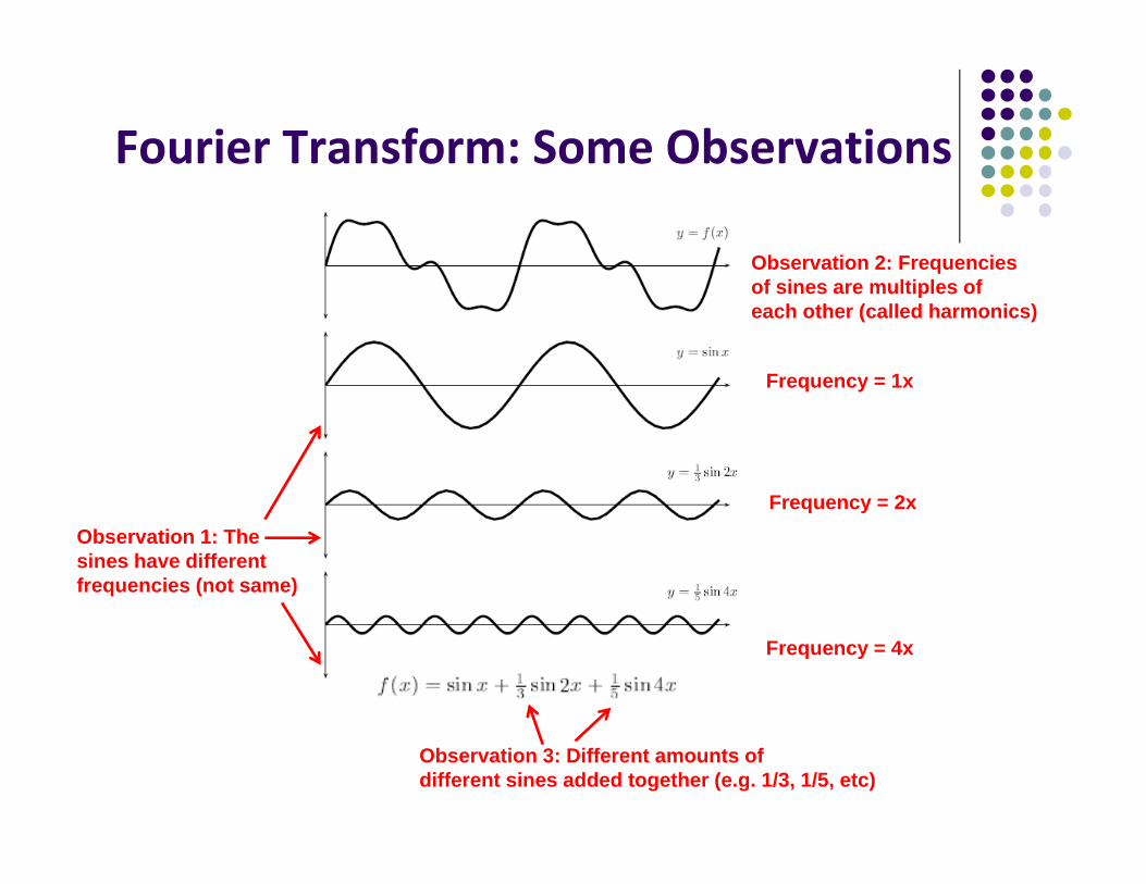
Fourier Transform: Some Observations

Observation 1: The sines have differentfrequencies (not same)

Observation 2: Frequenciesof sines are multiples ofeach other (called harmonics)

Frequency = 1x

Frequency = 2x

Frequency = 4x

Observation 3: Different amounts ofdifferent sines added together (e.g. 1/3, 1/5, etc)

Fourier Transform: Another Example

Square wave

ApproximationUsing sines

Observation 4: The sine terms go to infinity.The more sines we add, the closer theapproximation of the original.

Who is Fourier?

French mathematician and physicist

Lived 1768 ‐ 1830

Spectral Techniques

Technique for representation and analysis of signals in frequency domain including audio, images, video

How to decompose signal into summation of a series of sine and cosine functions (also called harmonic functions)

Spectral techniques can improve efficiency of image processing

Some image processing effects, concepts, techniques easier in frequency domain

Includes fourier transform, discrete fourier transform and discrete cosine transform

Sine and Cosine Functions: A Review Cosine function

A function is periodic if

Sines and cosines at different frequencies

Frequency = 1x Frequency = 3x

Sines and Cosines: A Review

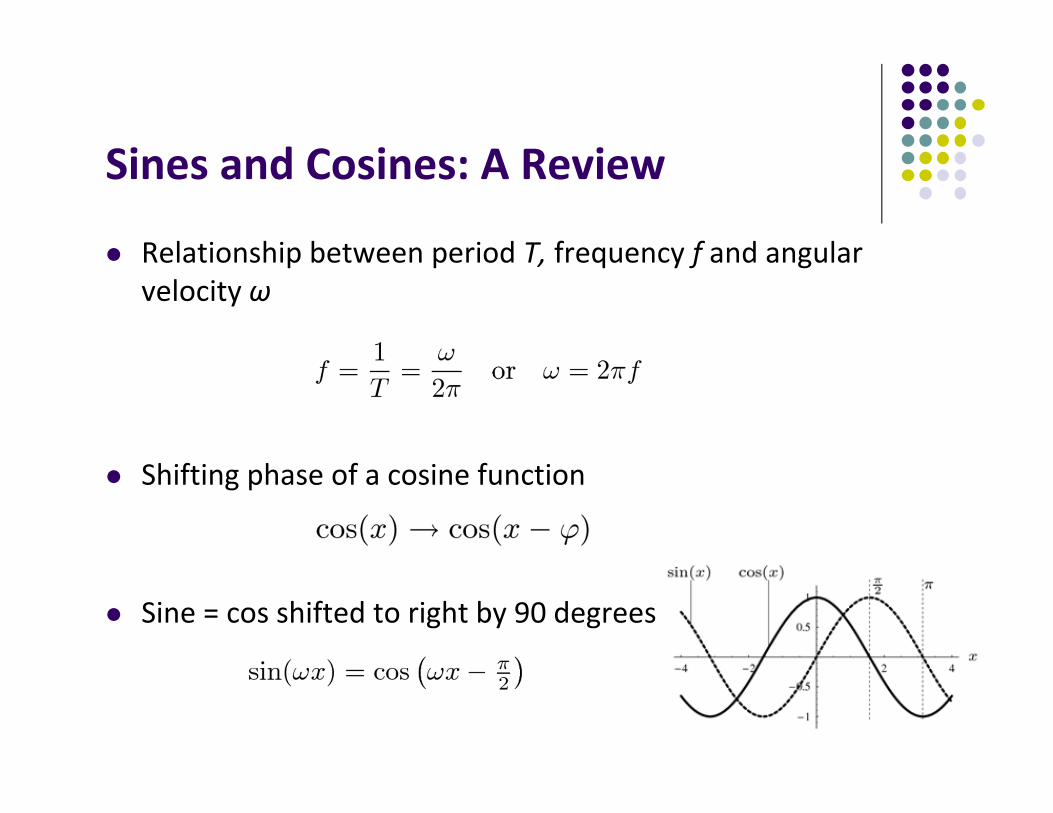
Relationship between period T, frequency f and angular velocity ω

Shifting phase of a cosine function

Sine = cos shifted to right by 90 degrees

Sines and Cosines: A Review

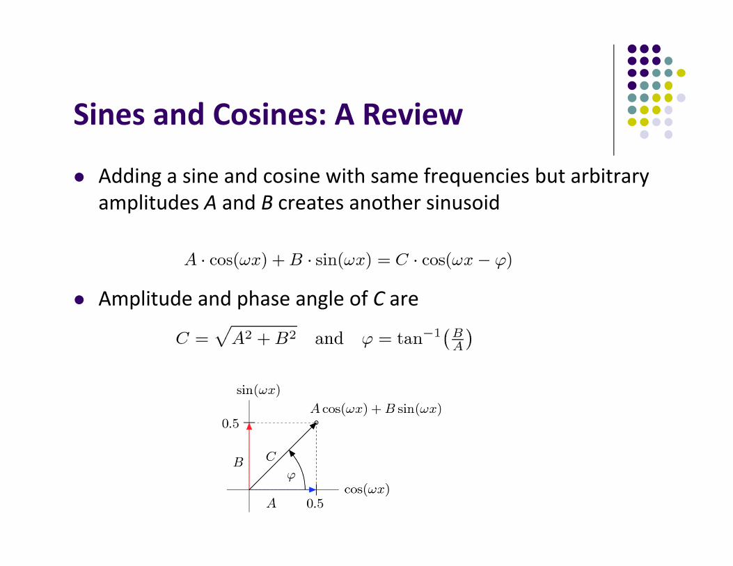
Adding a sine and cosine with same frequencies but arbitrary amplitudes A and B creates another sinusoid

Amplitude and phase angle of C are

Sines and Cosines: A Review

Euler’s complex number notation

Easy to combine sines and cosines of same frequency

Fourier Series of Periodic Functions

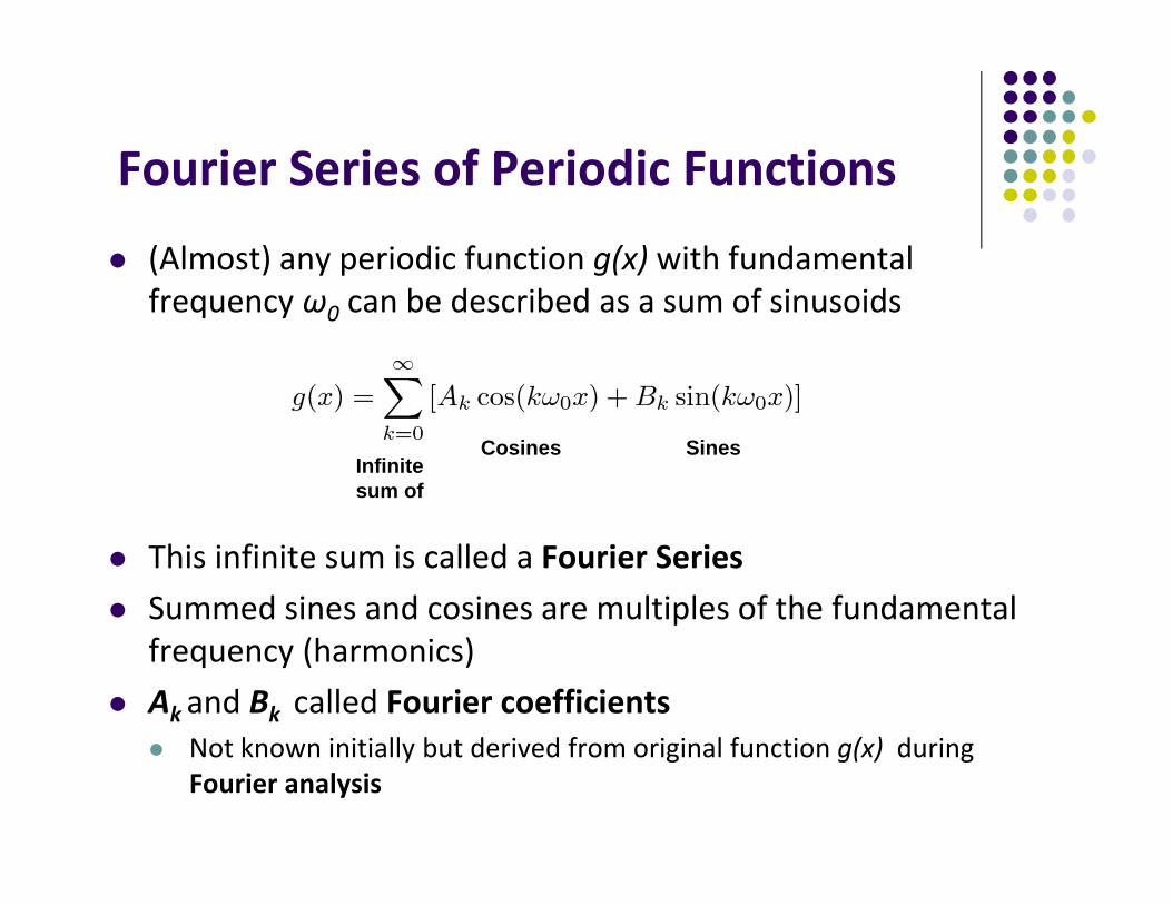
(Almost) any periodic function g(x) with fundamental frequency ω0 can be described as a sum of sinusoids 

This infinite sum is called a Fourier Series Summed sines and cosines are multiples of the fundamental 

frequency (harmonics) Ak and Bk  called Fourier coefficients

Not known initially but derived from original function g(x) during Fourier analysis

Infinitesum of

Cosines Sines

Fourier Integral

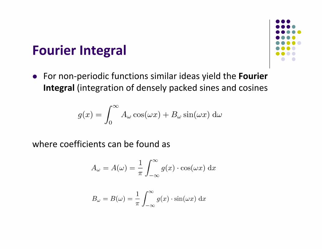
For non‐periodic functions similar ideas yield the Fourier Integral (integration of densely packed sines and cosines

where coefficients can be found as

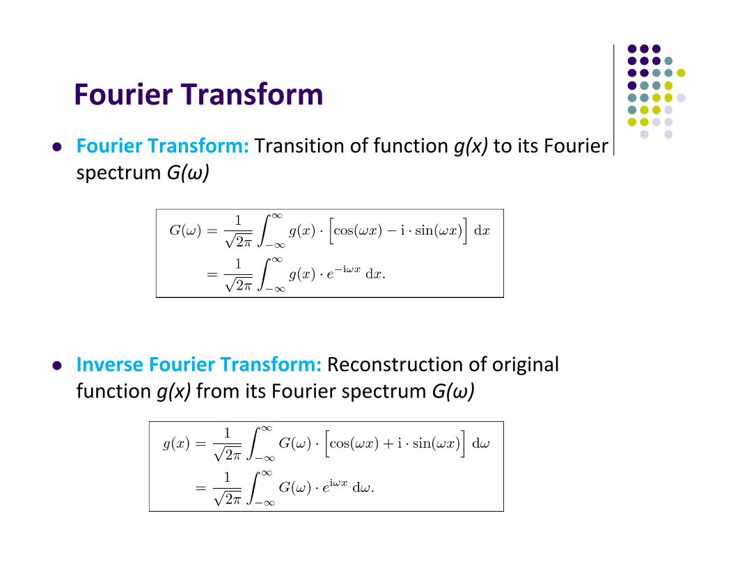
Fourier Transform Fourier Transform: Transition of function g(x) to its Fourier 

spectrum G(ω)

Inverse Fourier Transform: Reconstruction of original function g(x) from its Fourier spectrum G(ω)

References Wilhelm Burger and Mark J. Burge, Digital Image Processing, 

Springer, 2008 University of Utah, CS 4640: Image Processing Basics, Spring 

2012 Rutgers University, CS 334, Introduction to Imaging and 

Multimedia,  Fall 2012 Gonzales and Woods, Digital Image Processing (3rd edition), 

Prentice Hall Computer Graphics Using OpenGL 2nd edition by F.S Hill Jr, 

chapter 12