digital power regulation...

Digital PowerRegulation Solutions

Instructor:Tom Spohrer,

Product Marketing Manager,MCU16 Division, Microchip Technology, Inc.

HOUSEKEEPING• Housekeeping• Presentation• Text Chat Questions and Answers• Wrap-up

Agenda

Review the Levels of Digital Integration

Benefits of Full Digital Control

Digital Controller Basics

Analog SMPS and Digital SMPS Implementations

The Digital PID

The Mathematics, Generating the Coefficients, DSC Digital PID Implementation

Typical DSC Firmware Architecture

Other Digital Compensator Types

Advanced Digital Control

Adaptive, Non-linear, and Predictive algorithms

Additional Resources

App Notes, Libraries, Digital Compensator Design Tool, Workshops

Levels of Digital Integration

Level 1: Control improves traditional

analog power design Soft-start and Power Sequencing

Voltage and Temperature Monitoring

Communication and Data Logging





Level 2: MCU controls reference signals

for the PWM Controller Indirectly Set Voltage, Current and Thermal Limits

Determine PWM Period and Max Duty Cycle

Self-calibration










Self-calibration

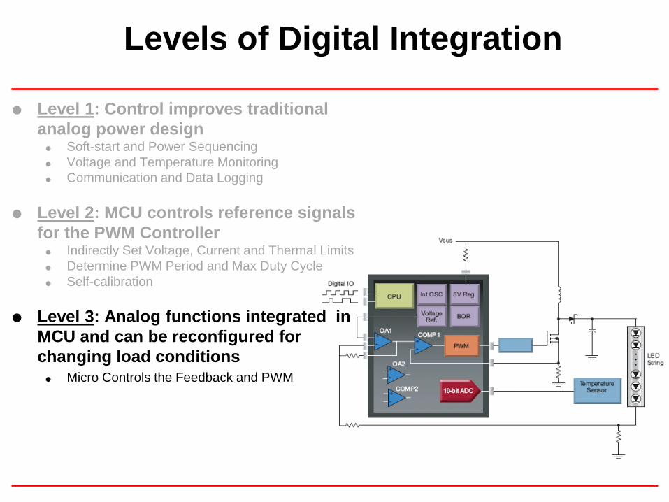
Level 3: Analog functions integrated in

MCU and can be reconfigured for

changing load conditions Micro Controls the Feedback and PWM









Self-calibration

Level 3: Analog functions integrated in

MCU and can be reconfigured for

changing load conditions Micro Controls the Feedback and PWM

Level 4: Analog feedback is replaced

with complete digital DSP-based control PID, 2P2Z, 3P3Z Algorithms with Voltage or Current

Mode Control Digital Signal Controller

V IN

Gate Driver

L

CoD 1

Q1

ADCDigital Compensator

Reference

DPWM

VOUT

Technical Advantages

of Digital Control

Software-driven controllers can implement any topology

Non-linear, predictive, and adaptive control techniques can be implemented for highest efficiency across widely varying load and environmental conditions

Change topology “On-the-Fly”: e.g. multi-phase to single phase at low-load to optimize efficiency

Minimize over-specification of magnetic components because DSC provides tighter tolerance than passive Rs & Cs

Reduced BOM costs

Fewer components result in higher power densitiesand higher reliability

Business Advantages

of Digital Control

IP belongs to PS vendor & resides in secured firmware

Fewer hardware platforms support more products

Easily update software to meet changing customer needs

Improved self-test capability simplifies product testing

Component tolerance & drift reduced:

(Eliminate “Over specified” components)

Restrict products from operating beyond specification

Log any misuse in the advent of warranty return

ReferenceCompensator

Hc

SystemPlantHsys

Error Output

Feedback GainHFB

+-

Controller Basics

Reference: This is the desired set-point we want the Output to follow

Error: Calculation of (Reference – Feedback), this is the value the compensator acts upon

Compensator: Digital compensator (PID, 2P2Z, 3P3Z, or 4th order, etc.)

System: This is the System/Plant/Power stage being controlled (SMPS, Motor, Actuator, etc)

Output: For our purposes this will be Voltage or Current

Feedback: The measurement of the output signal level

FBsysc

sysc

clHHH

HHsG

1)(

VIN VOUT

+

-

+

-

Comparator

Reference

Gate Driver

C2

C1 R2 R3

R1

C3

L

Co

Rf1

Rf2

D1

Q1

Analog PWM SMPS

Implementation

Analog Type III Compensator + PWM

Plant

Feedback

Analog Generator

Edge Aligned PWM

PWM Period

Error Amplifier Output (VEA)

Analog PWM Generator

T

ONTD

ONTT

VIN VOUT

+

-

+

-

Comparator

Reference

Gate Driver

C2

C1 R2 R3

R1

C3

L

Co

Rf1

Rf2

D1

Q1

Analog PWM SMPS

Implementation

Analog Type III Compensator + PWM

Plant

Feedback

Microchip dsPIC

VIN

Gate Driver

L

CoD1

Q1

ADCDigital Compensator

Reference

DPWM S/H

VOUT

Rf1

Rf2

Digital PWM SMPS

Implementation

Digital Signal Controller

Plant

Feedback

Digital Compensator + DPWM

Example Digital Signal

Controller for Digital Power

Digital Power Peripherals

12-bit ADCs - 5 (up to 22 Channels)

UART - 2

Analog Comp - 4 (with 12-bit DACs)

Programmable Gain Amplifiers - 2

Input Capture - 4

Output Compare - 4

I2C™ - 2 with PMBus™ Support

SPI - 2

UART - 2

Analog Comp. - 4 (with 12-bit DACs)

Programmable Gain Amplifiers - 2

Input Capture - 4

SMPS PWM - 10 Channels, 5 Pairs

Output Compare - 4

16-bit Timers - 5

I2C - 2 with PMBus Support

SPI - 2

SMPS PWM - 10 Channels, 5 Pairs

16-bit Timers - 5

12-bit ADCs - 5 (up to 22 Channels)

MEMORY BUSP

ER

IPH

ER

AL

BU

S

16 – 64KB

Flash with

Live Update

8KB RAM

Pe

rip

he

ral P

in S

ele

ct

MEMORY BUS

Operating Temperature: -40 to 125 °C

PE

RIP

HE

RA

L B

US

16 – 64 KB

Flash with

Live Update

2 – 8 KB

RAM

Pe

rip

he

ral P

in S

ele

ct

Digital Signal Controller

Microcontroller

Fast interrupt response time

DSP features

High resolution accumulators

The PID Controller


Hc

SystemPlantHsys

Error Output

Feedback GainHFB

+-

u

PROPORTIONAL

TERM

INTEGRAL

TERM

DERIVATIVE

TERM

PID Controller

u

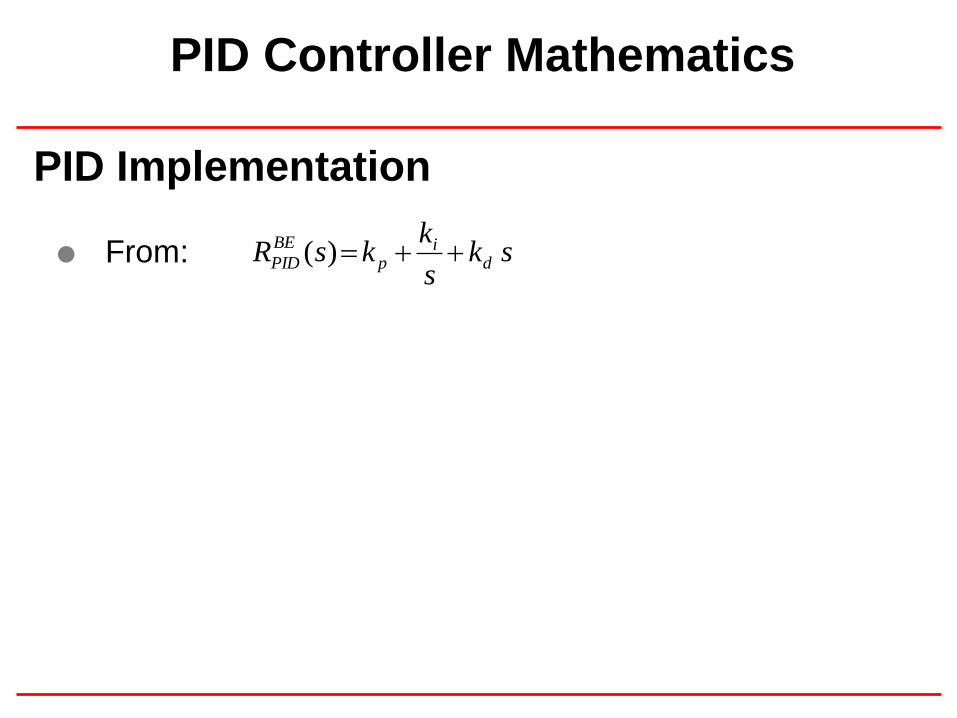
PID Controller Mathematics

PID Implementation

sks

kksR d

ip

BE

PID )( From:

PID Implementation

zT

zs

1

sks

kksR d

ip

BE

PID )( From:

Using: (Backward Euler)


PID Implementation

1

21

1

2

z

zT

kz

T

kk

T

kTkk

zR

ddp

dip

BE

PID

zT

zs

1

sks

kksR d

ip

BE

PID )( From:

Using: (Backward Euler)

We get:


PID Implementation

1

21

1

2

z

zT

kz

T

kk

T

kTkk

zR

ddp

dip

BE

PID

2121

ne

T

kne

T

kkne

T

kTkknunu dd

pd

ip

Z-Domain:

Time

Domain:


PID Implementation

1

21

1

2

z

zT

kz

T

kk

T

kTkk

zR

ddp

dip

BE

PIDZ-Domain:

Time

Domain:

Constants

2121

ne

T

kne

T

kkne

T

kTkknunu dd

pd

ip

KA KB KC


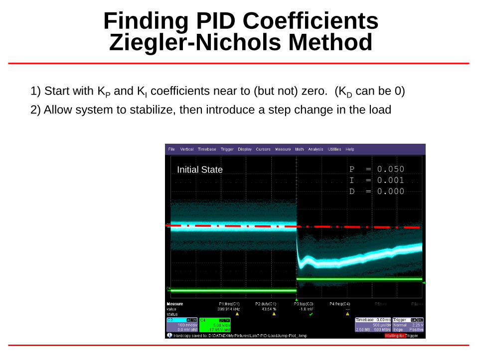
P = 0.050

I = 0.001

D = 0.000

Initial State

1) Start with KP and KI coefficients near to (but not) zero. (KD can be 0)

2) Allow system to stabilize, then introduce a step change in the load

Finding PID CoefficientsZiegler-Nichols Method

P = 0.180

I = 0.001

D = 0.000

Proportional Component

3) Increase KP until the tiny overshoot reaches the output voltage level and

then reduce it to approx. 70% of its value


P = 0.180

I = 0.028

D = 0.000

Integral Component

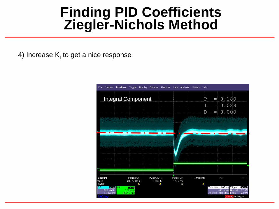
4) Increase KI to get a nice response


P = 0.180

I = 0.028

D = 0.042

Differential Component

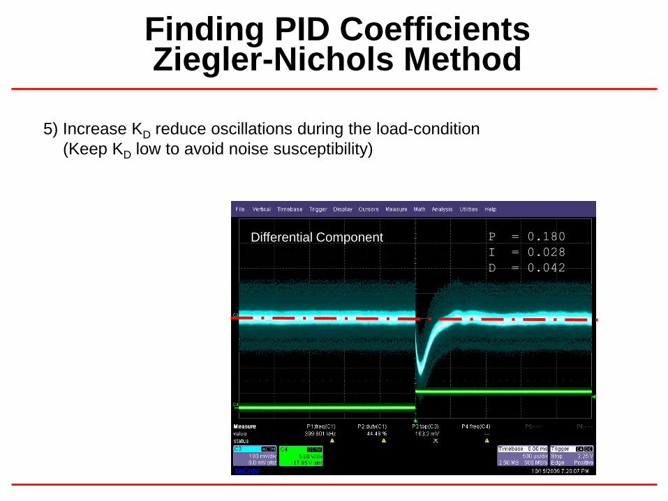
5) Increase KD reduce oscillations during the load-condition

(Keep KD low to avoid noise susceptibility)



PID Implementation

1

21

1

2

z

zT

kz

T

kk

T

kTkk

zR

ddp

dip

BE

PIDZ-Domain:

Time

Domain:

Constants

2121

ne

T

kne

T

kkne

T

kTkknunu dd

pd

ip

KA KB KC

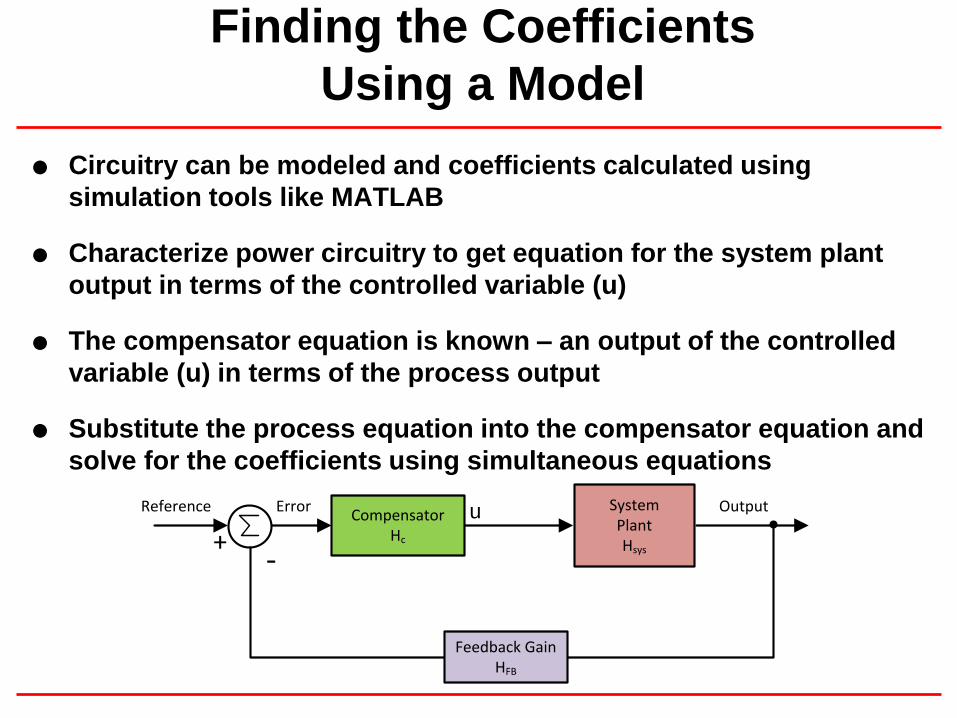
Circuitry can be modeled and coefficients calculated using

simulation tools like MATLAB

Characterize power circuitry to get equation for the system plant

output in terms of the controlled variable (u)

The compensator equation is known – an output of the controlled

variable (u) in terms of the process output

Substitute the process equation into the compensator equation and

solve for the coefficients using simultaneous equations

Finding the Coefficients

Using a Model


Hc

SystemPlantHsys

Error Output

Feedback GainHFB

+-

u

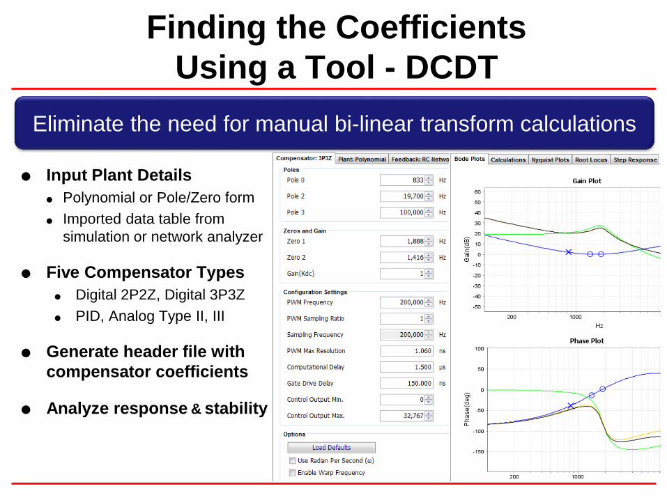
Finding the Coefficients

Using a Tool - DCDT

Eliminate the need for manual bi-linear transform calculations

Input Plant Details

Polynomial or Pole/Zero form

Imported data table from

simulation or network analyzer

Five Compensator Types

Digital 2P2Z, Digital 3P3Z

PID, Analog Type II, III

Generate header file with

compensator coefficients

Analyze response & stability


PID Implementation

1

21

1

2

z

zT

kz

T

kk

T

kTkk

zR

ddp

dip

BE

PIDZ-Domain:

Time

Domain:

Constants

2121

ne

T

kne

T

kkne

T

kTkknunu dd

pd

ip

KA KB KC

MAC w6*w7, A, [w8]+=2, w6, [w10]-=4, w7, [w13]+=2

One instruction,

One clock cycle,

8 operations

One

instruction,

One clock

cycle

One instruction performs:A = W6 * W7 ; W6 multiplied by W7 and product added to A

W6 = (W8) ; load new data addressed by W8 into W6

W7 = (W10) ; load new data addressed by W10 into W7

W8 = W8+2 ; Add 2 to address in W8

W10 = W10-4 ; Subtract 4 from address in W10

(W13) = B ; Copy B (rounded) to memory specified by W13

W13 = W13+2 ; Increment W13 by 2

MAC Instruction

DSC Digital PID

PIDs in DSCs: Architecture

ACC

Coefficients Error InputsRAM

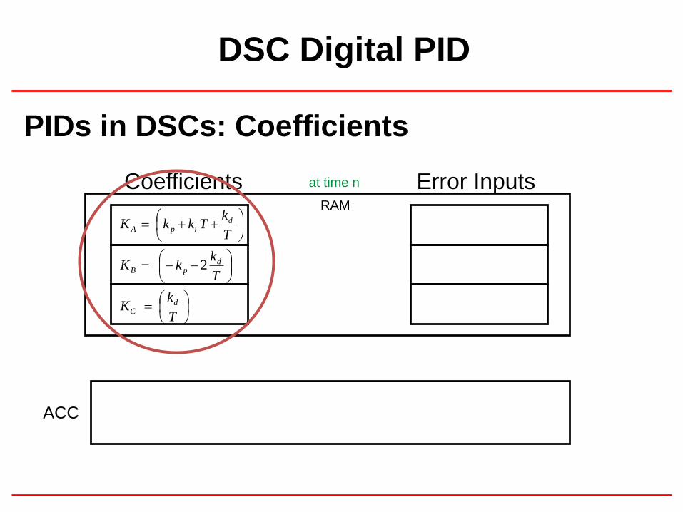
PIDs in DSCs: Coefficients

ACC

Coefficients Error Inputs

T

kK

T

kkK

T

kTkkK

dC

dpB

dipA

2

RAM

at time n

DSC Digital PID

PIDs in DSCs: New Error Value

ACC

2

1

ne

ne

ne


T

kK

T

kkK

T

kTkkK

dC

dpB

dipA

2

RAM

at time n NEW ERROR

VALUE

DSC Digital PID

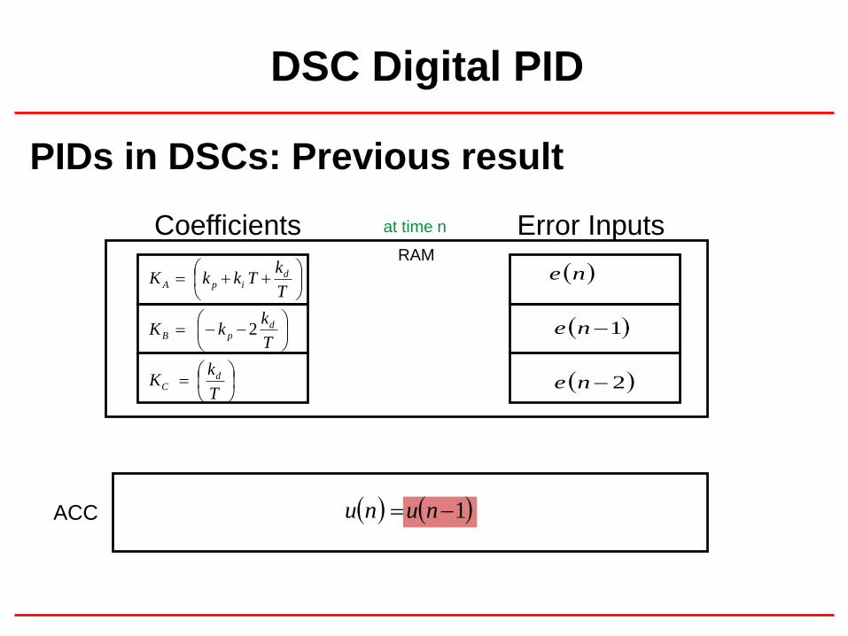
PIDs in DSCs: Previous result

ACC 1 nunu

2

1

ne

ne

ne


T

kK

T

kkK

T

kTkkK

dC

dpB

dipA

2

RAM

at time n

DSC Digital PID

neT

kTkknunu d

ip

1

PIDs in DSCs: First Contribution

ACC

2

1

ne

ne

ne


T

kK

T

kkK

T

kTkkK

dC

dpB

dipA

2

RAM

at time n

MAC instruction Total number of instruction cycles: 1

DSC Digital PID

121

ne

T

kkne

T

kTkknunu d

pd

ip

PIDs in DSCs: Second Contribution

ACC

2

1

ne

ne

ne


T

kK

T

kkK

T

kTkkK

dC

dpB

dipA

2

RAM

at time n


DSC Digital PID

2121

ne

T

kne

T

kkne

T

kTkknunu dd

pd

ip

PIDs in DSCs: Third Contribution

ACC

2

1

ne

ne

ne


T

kK

T

kkK

T

kTkkK

dC

dpB

dipA

2

RAM

at time n


DSC Digital PID

2121

ne

T

kne

T

kkne

T

kTkknunu dd

pd

ip

PIDs in DSCs: Updated result

ACC

2

1

ne

ne

ne


T

kK

T

kkK

T

kTkkK

dC

dpB

dipA

2

RAM

at time n


Digital PID Equation

DSC Digital PID

PIDs in DSCs: Ready for Next Iteration

ACC

1ne

ne


T

kK

T

kkK

T

kTkkK

dC

dpB

dipA

2

RAM

at time n + 1

2121

ne

T

kne

T

kkne

T

kTkknunu dd

pd

ip

empty location

DSC Digital PID

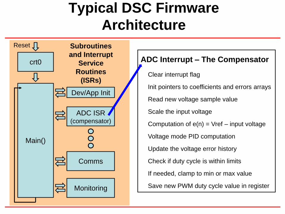
Typical DSC Firmware

Architecture

crt0

Main()

ADC ISR(compensator)

Monitoring

Reset

Comms

Dev/App Init

Subroutines

and Interrupt

Service

Routines

(ISRs)

crt0

Main()


Monitoring

Reset

Comms

Dev/App Init

Subroutines

and Interrupt

Service

Routines

(ISRs)

Device / Application Initialization

InitClock(); Setup DSC oscillator and clock

InitComp(); Setup current limit comparator

InitADC(); Setup ADC for output voltage

sampling

InitPWM(); Setup PWM

InitIO(); Setup I/O

InitPID(); Initialize compensator, setup

pointers, clear error and output

history


Architecture

crt0

Main()


Monitoring

Reset

Comms

Dev/App Init

Subroutines

and Interrupt

Service

Routines

(ISRs)

ADC Interrupt – The Compensator

Clear interrupt flag

Init pointers to coefficients and errors arrays

Read new voltage sample value

Scale the input voltage

Computation of e(n) = Vref – input voltage

Voltage mode PID computation

Update the voltage error history

Check if duty cycle is within limits

If needed, clamp to min or max value

Save new PWM duty cycle value in register


Architecture

Digital Implementation of a Control Loop

ADC

Controller Computation

(ADC ISR)

PWM Delay

PWM Period

T1

T2

T3

Tdelay

Change can become

effective during the following

PWM period if delay exceeds

start of next PWM cycle

TRIGGER

Delay from sample point to

PWM update results in

reduction of phase margin

Control Loop Timing

Digital Compensator Types

Proportional Integral Derivative (PID)

Most common compensator type in industrial control applications,

although not ideal for SMPS applications

Uses only three coefficients – simple method to find the values

Only compensates one pole and one zero of plant

Digital 2P2Z (similar to Analog Type II)

Five coefficients – Five MAC instructions to calculate

Current-mode converters

Digital 3P3Z (similar to Analog Type III)

Seven coefficients – Seven MAC instructions to calculate

Voltage-mode buck or boost-derived converters

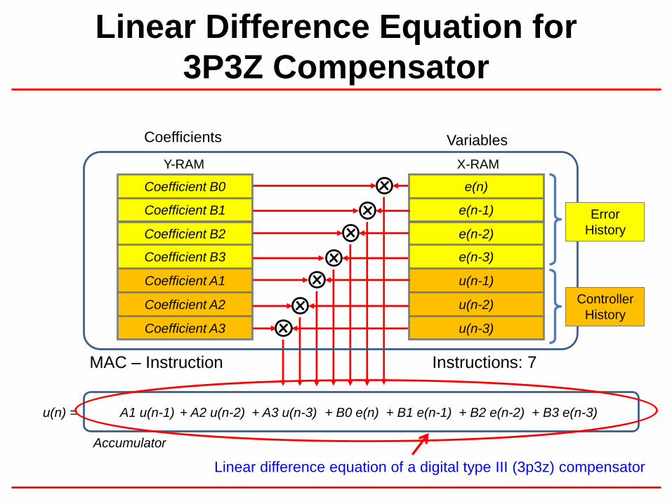
Coefficients Variables

Accumulator

Coefficient B0

Coefficient B1

Coefficient B2

Coefficient B3

Coefficient A1

Coefficient A2

Coefficient A3

e(n)

e(n-1)

e(n-2)

e(n-3)

u(n-1)

u(n-2)

u(n-3)

Y-RAM X-RAM

MAC – Instruction Instructions: 7

Error

History

Controller

History

u(n) = + B3 e(n-3)+ B2 e(n-2)+ B1 e(n-1)+ B0 e(n)+ A3 u(n-3)+ A2 u(n-2)A1 u(n-1)

Linear difference equation of a digital type III (3p3z) compensator

Linear Difference Equation for

3P3Z Compensator

Full Digital Control

Adaptive Algorithms

Improving Efficiency over widely varying loads

Phase shedding

Dead-time adjustment

Variable switching frequency

Variable bulk voltage Energy Star Efficiency Requirements

Full Digital Control Predictive

and Non-linear Algorithms

j=30°

j=60°

j=-30°

j=- 60°

Steady StateLinear compensator such as 3P3Z

Decay / BoostModify compensator output by

non-linear factor(s)

AttackOverride compensator results

with min/max values for a limited

number of cycles

Dynamic Responsiveness

Non-linear Algorithms

Real-time coefficient scaling

Predictive Algorithms

Bypass damping of control loops

j represents a vector:

Sum of the absolute

value of 3 error samples

vs 0 degree vector

representing errors

averaging zero

DS70336 – Buck/Boost Converter PICtail User Guide

AN1114 – Switch Mode Power Supply Topologies (Part I)

AN1207 – Switch Mode Power Supply Topologies (Part II)

AN1106 – Power Factor Correction

DS70320 – dsPIC SMPS AC-DC Reference Design User Guide

AN1278 – Interleaved Power Factor Correction

AN1279 – 1000VA Off-line UPS

AN1335 – Quarter Brick PSFB DC/DC

AN1336 – LLC DC/DC

AN1338 – Grid-Connected Solar Micro-Inverter

SMPS Application Notes / Guides

SMPS Compensator Libraries

3P3Z, 2P2Z, and PID Compensators

Good compromise between speed vs. resolution

3P3Z takes ~ 1.6us, 2P2Z takes ~1.4us

Compensators written to support MATLAB code

generation (future)

MATLAB needs specific Inputs and Outputs to be defined

void SMPS_Controller3P3ZUpdate(SMPS_3P3Z_T*

controllerData, volatile uint16_t* controllerInputRegister,

int16_t reference, volatile uint16_t* controllerOutputRegister);

Pointer to structure (min/max clamps, pre/post shifts, coefficients, and

control/error history)

Pointer to control input (i.e. ADCBUFx)

Control Reference

Pointer to control output (PDCx, CMPDACx, etc.)

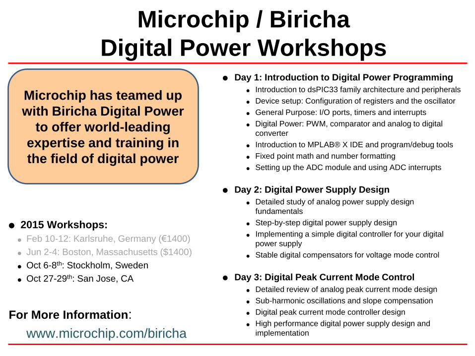
Microchip / Biricha

Digital Power Workshops

2015 Workshops:

Feb 10-12: Karlsruhe, Germany (€1400)

Jun 2-4: Boston, Massachusetts ($1400)

Oct 6-8th: Stockholm, Sweden

Oct 27-29th: San Jose, CA

For More Information:

www.microchip.com/biricha

Day 1: Introduction to Digital Power Programming

Introduction to dsPIC33 family architecture and peripherals

Device setup: Configuration of registers and the oscillator

General Purpose: I/O ports, timers and interrupts

Digital Power: PWM, comparator and analog to digital

converter

Introduction to MPLAB® X IDE and program/debug tools

Fixed point math and number formatting

Setting up the ADC module and using ADC interrupts

Day 2: Digital Power Supply Design

Detailed study of analog power supply design

fundamentals

Step-by-step digital power supply design

Implementing a simple digital controller for your digital

power supply

Stable digital compensators for voltage mode control

Day 3: Digital Peak Current Mode Control

Detailed review of analog peak current mode design

Sub-harmonic oscillations and slope compensation

Digital peak current mode controller design

High performance digital power supply design and

implementation

Microchip has teamed up

with Biricha Digital Power

to offer world-leading

expertise and training in

the field of digital power

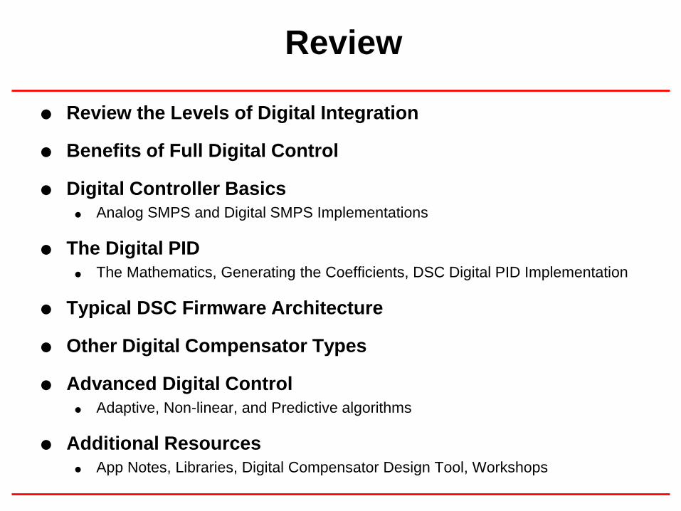
Review

Review the Levels of Digital Integration

Benefits of Full Digital Control

Digital Controller Basics

Analog SMPS and Digital SMPS Implementations

The Digital PID

The Mathematics, Generating the Coefficients, DSC Digital PID Implementation

Typical DSC Firmware Architecture

Other Digital Compensator Types

Advanced Digital Control

Adaptive, Non-linear, and Predictive algorithms

Additional Resources

App Notes, Libraries, Digital Compensator Design Tool, Workshops

Audience Q & Avia Chat

IF YOU DO NOT SEE THE CHAT MODULE ON YOUR SCREEN,

Click here to join us for the class chat:http://opsy.st/1QUoTGw

Instructor:Tom Spohrer, Product Marketing Manager,MCU16 Division,Microchip Technology, Inc.

Moderator:Rich Nass, EVP, OpenSystems Media

http://opsy.st/1QUoTGw

Thanks for joining us

Class archive available at:http://opsy.st/1QUoTGw

E-mail us at: [email protected]

http://opsy.st/1QUoTGw

digital power regulation...

Documents