digital seismo-acoustic signal processing aboard a

University of New Hampshire University of New Hampshire

University of New Hampshire Scholars' Repository University of New Hampshire Scholars' Repository

Master's Theses and Capstones Student Scholarship

Winter 2007

Digital seismo-acoustic signal processing aboard a wireless Digital seismo-acoustic signal processing aboard a wireless

sensor array for volcano monitoring sensor array for volcano monitoring

Omar E. Marcillo University of New Hampshire, Durham

Follow this and additional works at: https://scholars.unh.edu/thesis

Recommended Citation Recommended Citation Marcillo, Omar E., "Digital seismo-acoustic signal processing aboard a wireless sensor array for volcano monitoring" (2007). Master's Theses and Capstones. 337. https://scholars.unh.edu/thesis/337

This Thesis is brought to you for free and open access by the Student Scholarship at University of New Hampshire Scholars' Repository. It has been accepted for inclusion in Master's Theses and Capstones by an authorized administrator of University of New Hampshire Scholars' Repository. For more information, please contact [email protected].

https://scholars.unh.edu/

https://scholars.unh.edu/thesis

https://scholars.unh.edu/student

https://scholars.unh.edu/thesis?utm_source=scholars.unh.edu%2Fthesis%2F337&utm_medium=PDF&utm_campaign=PDFCoverPages

https://scholars.unh.edu/thesis/337?utm_source=scholars.unh.edu%2Fthesis%2F337&utm_medium=PDF&utm_campaign=PDFCoverPages

mailto:[email protected]

DIGITAL SEISMO-ACOUSTIC SIGNAL PROCESSING ABOARD A WIRELESS

SENSOR ARRAY FOR VOLCANO MONITORING

BY

OMAR E. MARCILLO

B.S., Escuela Politecnica Nacional, 2002

THESIS

Submitted to the University of New Hampshire

In Partial Fulfillment of

The Requirements for the Degree of

Master of Science

In

Earth Sciences: Geology

December, 2007

R eproduced with perm ission of the copyright owner. Further reproduction prohibited without perm ission.

UMI Number: 1449595

UMIUMI Microform 1449595

Copyright 2008 by ProQuest Information and Learning Company. All rights reserved. This microform edition is protected against

unauthorized copying under Title 17, United States Code.

ProQuest Information and Learning Company 300 North Zeeb Road

P.O. Box 1346 Ann Arbor, Ml 48106-1346


This thesis has been examined and approved.

Thesis )irector, Jeffrey B. Johnson, Research Assistant Professor ofEarth Sciences

Francis S. Birch, Professor of Earth Sciences

Andrew L. Kun, Associate Professor of Electrical and ComputerEngineering

Matt Welsh, Associate Professor of Computer Sciences,Harvard University

Date


DEDICATION

This thesis is dedicated to my parents Sonia and Segundo who have taught me to

live, the most important lesson in my life1.

1 Esta tesis esta dedicada a mis padres Sonia y Segundo quienes me han ensenado

a vivir, la leccion mas importante de mi vida.

iii


ACKNOWLEDGEMENTS

I thank Jeff Johnson for being such a supportive, patient, and dedicated advisor and

for being my friend. I thank the members of my committee; Prof. Brancis Birch, Prof.

Andrew Kun, and Prof. Matt Welsh for generously offering their time, expertise, and

guidance throughout the development of this thesis. I thank Geoff and Konrad from the

research group of Prof. Welsh at Harvard University for reviewing the code I am using in

this system.

I am grateful to all the friends I met in USA, they showed me a great culture and

let me be part of it. I want to express all my gratitude to Gerry, Jason, Tom, Abby, Rene,

and Joe for their friendship. I want to thank Eileen from the bottom of my heart for being

such an important and beautiful part of my life. I want to thank all my family for their

support Sonia, Segundo, Veronica, Pablo, Andrea, Alejo, Vidar, Melli, and Isabela. I

want to give many thanks to Daniela for being always in my thoughts.

This work was supported through grants from the National Science Foundation

(NSF EAR 0440225) and the President's Excellence Initiative through the office of the

Vice President for Research and Public Service at the University of New Hampshire.

iv


TABLE OF CONTENTS

DEDICATION........................................................................................................................iii

ACKNOWLEDGEMENTS.................................................................................................... iv

LIST OF TABLES................................................................................................................ vii

LIST OF FIGURES.............................................................................................................. viii

ABSTRACT............................................................................................................................ ix

CHAPTER PAGE

INTRODUCTION....................................................................................................................1

1. VOLCANIC ERUPTIONS AND MONITORING....................................................4

Volcanic Eruptions.......................................................................................................4Explosive Volcanic Eruptions.........................................................................5Energy Budget In Volcanic Eruptions...........................................................6

Volcano Monitoring.....................................................................................................7Small Aperture Arrays.................................................................................... 8

2. DIGITAL SIGNAL PROCESSING ON WIRELESS SENSOR NETWORKS .. 12

Wireless Sensor Network For Volcano Monitoring................................................13A WSN at Tungurahua Volcano...................................................................13A WSN at El Reventador Volcano.............................................................. 14

Digital Seismic Processing........................................................................................17Phase Detectors And Phase Pickers............................................................. 19Time-Domain Event Detectors.................................................................... 20The STA/LTA Algorithm.............................................................................21

Continuous Seismic Monitoring On Volcanoes..................................................... 25Digital Filters.................................................................................................27

v


3. DESCRIPTION OF THE WIRELESS SENSOR ARRAY..................................... 29

Wireless Seismo-Acoustic Array: Hardware Characteristics................................. 29The sensor nodes........................................................................................... 30Conditioning Board....................................................................................... 31Time synchronization node.......................................................................... 34The base node................................................................................................34

Data Analysis Description........................................................................................ 35

Laboratory Test Results............................................................................................ 40

4. CONCLUSIONS, RECOMMENDATIONS, FIELD DEPLOYMENT ANDFUTURE WORK............................................................................................................. 44

Conclusions and Recommendation.......................................................................... 44

Field deployment.......................................................................................................46

Future Work.............................................................................................. 46

REFERENCES.......................................................................................................................48

APPENDICES........................................................................................................................55

Appendix A: Electronic Diagram Of The Conditioning Board..............................56

Appendix B: The “Dataanalysis” Component Source Code...................................59

vi


LIST OF TABLES

Table 1: Different configuration of STA/LTA algorithms................................................ 25

Table 2: Description of the variables of the message activityMsg.................................... 38

Table 3: Parameters of the STA/LTA algorithm................................................................39

Table 4: Description of the variables of the message eventMsg.......................................40

vii


LIST OF FIGURES

Figure 1: Cartoon showing a plane wave moving across an array of sensors.................. 10

Figure 2: Mica2 mote and conditioning board for the electret microphone.......................14

Figure 3: Network topology of the seismo-acoustic array at El Reventador volcano 15

Figure 4: Sensor node distribution on the field deployment at El Reventador volcano... 16

Figure 5: Event detector and event picker for a seismic signal...........................................19

Figure 6: Characteristic Functions........................................................................................ 22

Figure 7: Position of windows for STA/LTA algorithms................................................... 24

Figure 8: Frequency analysis of a seismic signal................................................................. 27

Figure 9: Elements and distribution of the elements of the seismo-acoustic array proposed

by this work............................................................................................................................. 30

Figure 10: The amplification stage of the conditioning board........................................... 33

Figure 11: Example of the Tmote Sky 12-bit ADC............................................................33

Figure 12: Elements and operation of the time synchronization and base node................ 35

Figure 13: Frequency and phase response 0-5 Hz low pass filter......................................36

Figure 14: Frequency and phase response 5-10 Hz band pass filter...................................37

Figure 15: RSAM and SSAM aboard the sensor node........................................................41

Figure 16: First arrival times calculated on the three sensor nodes....................................43

viii


ABSTRACT

DIGITAL SEISMO-ACOUSTIC SIGNAL PROCESSING ABOARD A WIRELESS

SENSOR ARRAY FOR VOLCANO MONITORING

by

Omar E. Marcillo

University of New Hampshire, December, 2007

This work describes the design and implementation of a low cost wireless sensor array

utilizing digital processing to conduct autonomous real-time seismo-acoustic signal

analysis of earthquakes at actively erupting volcanoes. The array consists of 1) three

sensor nodes, which comprise seismic and acoustic sensors, 2) a GPS-based time

synchronization node, and 3) a base receiver node, which features a communication

channel for long distance telemetry. These nodes are based on the Moteiv TMote Sky

wireless platform. The signal analysis accomplishes Real-time Seismic-Amplitude

Measurement (RSAM) and Seismic Spectral-Amplitude Measurement (SSAM)

calculations, and the extraction of triggered arrival time, event duration, intensity, and a

decimated version of the triggered events for both channels. These elements are

fundamental descriptors of earthquake activity. The processed data from the sensor nodes

are transmitted back to the central node, where additional processing may be performed.

This final information can be transmitted periodically via low bandwidth telemetry

options.

ix


INTRODUCTION

A volcanic eruption is a phenomenon related to the transportation of volcanic

material (magma and gas) and heat from the Earth’s interior to the surface. The eruption

of a volcano is one of the most spectacular and at times destructive displays of natural

energy. The deformation of the volcano’s surface, the generation of seismic and acoustic

waves, and the emission of lava, pressurized gases and pyroclastic debris are some of the

expressions of the volcanic activity. The studying and monitoring of the volcanic

phenomena help us to understand the mechanisms of energy transport between the

Earth’s interior and the surface. Study and monitoring of volcanoes are also important for

understanding the relation between volcanoes and their surroundings. These surroundings

include other elements of the Earth system, such as the biosphere, cryosphere and

atmosphere. Volcanoes have a strong influence on human activity; thus the study of

volcanoes, their history and current state of restlessness, is an important and vital

component in disaster prevention and hazard mitigation.

Several techniques have been developed for monitoring and studying volcanoes.

Some techniques focus on the geophysical and others on the geochemical processes

related to eruptions. These techniques study different aspects of the volcano activity such

as ground deformation, seismicity, variation of gas composition, and electromagnetic and

temperature anomalies. Due to the complex nature of volcanoes, their study requires the

application of multiparametric techniques in order to have a better understanding of their

significance. Seismic monitoring is one of the most common and useful tools for volcano

1


monitoring and forecasting. Nearly every well-monitored volcanic eruption has been

preceded by changes in seismic activity. The study of seismic activity allowed to

successfully forecast 25 volcanic eruptions between 1980 to 2000 (McNutt, 2000). This

forecasting led, in many of the cases, to important disaster prevention. Geophones or

seismometers are the most common tool to study seismic activity. These sensors convert

ground motion, displacement or velocity, into an electric signal. Recent studies (Garces et

al., 2000; Johnson et al., 2005) have demonstrated that coupling seismic monitoring with

the study of infrasonic airwaves generated during volcanic explosion provides a better

characterization of explosion earthquakes. Pressure transducers have been used to study

the air-wave components of volcanic eruption. In order to improve the performance of a

single sensor (e.g.: geophone or pressure transducers) dense clusters of sensors, or arrays,

are commonly used in volcanic studies.

Since 1960, the use of seismic arrays has shown its usefulness in the precise

localization and characterization of complex seismic wavefields. These can be generated

by nuclear, chemical or volcanic explosions (La Rocca et al., 2001; Followil et al., 1997;

Rost et al., 2002). The use of sensor arrays involves the generation of large amounts of

data, making its maintenance, management, and analysis a challenge in terms of

hardware and computational capabilities. Recent studies have shown that the emerging

technology of wireless sensor networks can provide a solid hardware platform for the

development of sensor arrays, and fulfill many of the requirements of volcano monitoring

(Werner-Allen et al., 2005; Werner-Allen et al., 2006).

2


This study focuses on the development of digital signal processes for basic real

time in-situ analysis of seismo-acoustic signals, and its implementation on a sensor array

based on a wireless sensor platform. This in-situ analysis includes: 1) calculation of the

energy in representative bandwidths of the seismic wavefield, 2) basic signal feature

extraction through energy envelope characterizations, and 3) backazimuth calculation.

These extracted parameters may be used for increasing our understanding of volcano

dynamics and also for monitoring purposes, which is part of the motivation of this

project. The description of this system includes a discussion of previous work in this area

and also a detailed explanation of the hardware and algorithms involved in the signal

analysis.

3


CHAPTER 1

VOLCANIC ERUPTIONS AND MONITORING

Volcanic Eruptions

A volcanic eruption can be defined as the arrival of volcanic material at the

surface of the Earth (Simkin et al., 2000). However, not all events that transport volcanic

material to the surface have been considered an eruption. This definition can be enhanced

by constraining the material that is transported to a mixture of solid volcanic material

with any other elements in liquid or gas phases. The mechanisms and velocities of the

transportation of material to the surface determine different types of volcanic eruptions.

Two types of volcanic eruptions can be considered the extremes of a broad

spectrum of types of eruptions: explosive and effusive. Different types of eruptions are

neither exclusive of a single volcano nor a single eruption but can evolve, coexist or have

intermediate states. Internal and external factors control the behavior of volcanic

eruptions. These factors can be summarized in the mass flux, the level of fragmentation

of the material, and the interaction of the emerged material with the surroundings

(Zimanowski et al., 1997). Continuous behavior is displayed in effusive volcanic

eruptions. The system that was developed for this project focuses on the study of

explosive eruptions that tend to produce large inffasonic wave and have discrete

behavior.

4


Explosive Volcanic Eruptions

A dense mixture of ash and gas ejected at high speeds and pressures from a

volcanic vent is one the distinguishing characteristics of explosive volcanic eruptions

(Woods, 1995). This ejected material is a result of the explosion of gas bubbles (mainly

water vapor, carbon dioxide, sulfur dioxide) that are embedded in the magma. These

bubbles, which are embedded in the rising magma, explode when the film that envelopes

the gases is not able to expand as fast as the volume inside increases (Woods, 1995). This

increase in the volume of gases can be the result of external factors such as contact with

water reservoirs (phreato-magmatic fragmentation) or sudden decompression of

magmatic bubbles (magmatic fragmentation).

Phreato-magmatic fragmentation produces very explosive fragmentation. It

involves the interaction of magma and water, where the first has a higher temperature

than the second’s critical temperature (Buttner, 1998). This fragmentation relies on a

phenomenon called Molten Fuel Coolant Interaction. Four stages have been identified in

this multiphase and multicomponent mechanism: 1) the mingling of magma and water

with the presence of a vapor film that insulates the water, 2) the condensation of the

vapor film resulting on a quasi direct contact between water and magma, 3) the cooling of

magma and expansion of gas due to the direct contact that enhances heat transportation,

and 4) the deformation and a subsequent fracture of the melt (Buttner et al., 2002). The

fracturing feeds cold material to the hot magma and a positive feedback is established

which enhances the fragmentation. This mechanism tends to produce violent explosive

5


eruptions. Phreatomagmatic fragmentation is the main eruptive mechanism of tuff rings

and maars ( Buttner et al., 2002)

In magmatic fragmentation there is a rapid exosolution of gas, mainly water

vapor, trapped in magma. Magmatic fragmentation transforms liquid magma with

disperse gas bubbles to a gas with dispersed liquid drops of magma (Cashman et al.,

2000). The rapid exsolution of volatiles in magma is the result of a process of

decompression. This decompression can be triggered by a rapid ascent of magma or due

to unloading, e.g.: an edifice or dome collapse, or by new injection of magma.

Energy Budget In Volcanic Eruptions

Thermal and kinetic energy of ejected material from vents are substantially

greater than seismic energy and have been identified as the main components of energy

that are released during a volcanic eruption (Pyle, 1995). For example for the energy

budget for the eruption of Stromboli volcano was calculated by McGetchin et al. (1979).

Thermal energy accounts about 84% of the total energy. Most of this amount is

transferred to the walls of the volcano through processes of conduction, another about

10% is transferred to volcanic gases. Radiated heat from the vent and ejected particles

account for about 3%, and a small fraction of the total energy, 0.5%, is radiated as

seismic and infrasonic waves.

Explosive volcanic eruptions display a partitioning of energy through the ground

as seismic explosion signals and through the air as air shock or sound in the infrasonic

6


bandwidth (1-20 Hz). These infrasonic waves travel through the atmosphere and tend to

exhibit low atmospheric scattering and dissipation which allows them to be used as a

proxy for source processes at the vent ( Johnson et al., 2005). These air waves can be

recorded by the use of specialized microphones and pressure transducers sensitive to low

frequencies.

Volcano Monitoring

The monitoring of active volcanoes has a dual purpose, first to provide the

scientific data to study the structure and evolution of volcanoes, and second, to help

reduce the societal hazards related to volcano eruptions. Several techniques have been

developed to monitor volcanoes. Some techniques focus on the study of their geophysical

parameters and others focus on the geochemical behavior of them.

Geochemical monitoring of volcanoes involves the chemical analysis of gases and

water that directly or indirectly are related to the volcanic activity. This monitoring looks

for changes in the chemistry in the composition of volcanic fluids. Geochemical analysis

in volcanoes has been used extensively. Some of these techniques require the dangerous

task of sampling near volcanic vents, which more than once has resulted in injuries and

loss of lives. The system that is presented in this work is not focused on geochemical

analysis; however, seismo-acoustic studies of eruptions will help us to better understand

the degassing processes in the vent.

The geophysical techniques are often intended to study the movement of magma,

which the majority of the times results in fracturing of rocks or opening of cracks. In

7


many cases the movement of magma also generates surface deformation. The study of the

deformation in the vicinity of active volcanoes is an important technique to monitor

volcanoes. This technique has experienced a rapid evolution due to the recent

developments of new sensors and improvement in telecommunications. The electronic

distance measuring, GPS, and interferometric synthetic aperture radar technologies are

some of the tools that have been recently developed and successfully used to monitor

volcanoes (Dzurisin, 2003; Janssen, 2007; Janssen et al., 2001).

Volcano seismology is one of the most common and useful disciplines for

volcano monitoring and forecasting. Nearly every well-monitored volcanic eruption has

been preceded by changes in seismic activity. The study of this activity allowed

successful forecasts of 25 volcanic eruptions between 1980 to 2000; this forecasting also

led in many cases to important disaster prevention (McNutt, 2000). Moreover the study

of the seismicity on volcanoes has been used not only for surveillance but also for the

generation of physical models of volcanic phenomena, e.g.: Aki et al. (2000), Collombet

et al. (2003).

Small Aperture Arrays

Seismic arrays or seismic antennas are powerful tools for the study of wave fields

due to their ability to identify and separate wave field components with different

propagation properties (Almendros et al., 2002; Followil et al., 1997). Small aperture

arrays are based on the assumption that the wave that is moving across the array is a

plane wave. This technique has led to different applications including the study of

8


volcanic tremors and their source (Goldstein et al., 1994; Metaxian et al., 1997). Another

application is the separation of source and path effect in seismic studies (Almendros et

al., 2002). In a non-volcanic environment infrasonic and seismic arrays have been used

for monitoring nuclear explosions.

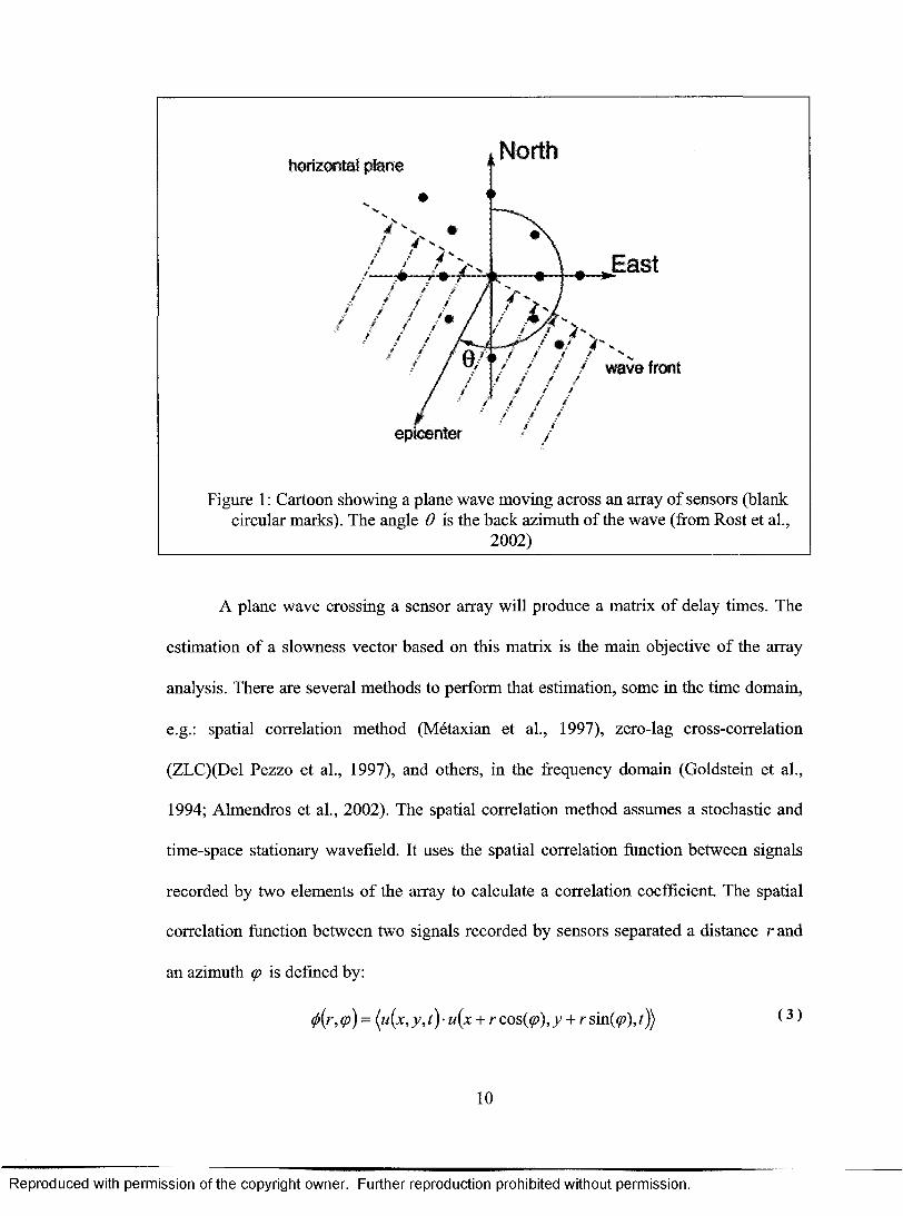
In order to understand a basic application of array techniques, we first imagine a

plane wave that moves across a surface (Figure 1) and define the slowness vector as a

vector that has a perpendicular direction to the wave front and a magnitude inverse to the

wave velocity. The slowness vector is mathematically represented as

where — and — are the inverse of the apparent horizontal and vertical velocity. Adx dz

plane wave (with a slowness vector s ) moving across a N-element array, will have an

arrival time equation to the i-th element of the array defined as,

where t0 is the arrival time of the wave to an element which is defined as the origin of

coordinates and rt is the position vector of the i-th element in relation to the origin of

coordinates. If the direction of the slowness vector is measured clockwise from the north,

this direction is the wave’s azimuth.

( l )

dt , dt

( 2 )

9


North

East

wave front

Figure 1: Cartoon showing a plane wave moving across an array of sensors (blank circular marks). The angle 0 is the back azimuth of the wave (from Rost et al.,

2002)

A plane wave crossing a sensor array will produce a matrix of delay times. The

estimation of a slowness vector based on this matrix is the main objective of the array

analysis. There are several methods to perform that estimation, some in the time domain,

e.g.: spatial correlation method (Metaxian et al., 1997), zero-lag cross-correlation

(ZLC)(Del Pezzo et al., 1997), and others, in the frequency domain (Goldstein et al.,

1994; Almendros et al., 2002). The spatial correlation method assumes a stochastic and

time-space stationary wavefield. It uses the spatial correlation function between signals

recorded by two elements of the array to calculate a correlation coefficient. The spatial

correlation function between two signals recorded by sensors separated a distance r and

an azimuth (p is defined by:

(f)(r, (p) = (u(x,y,t)- u(x + r cos(<p), y + r sin(^), tjj ( 3 )

10


where u(x,y ,t) is the signal recorded at the coordinates x and y, and at time t and the

angle brackets represent time averaging. The correlation coefficient is defined by

Metaxian et al. (1997):

/ s 0(r,<p,o)o)P \r , (p,a}0) — —t t r (4 )

where coQ is the center of a narrow band of frequencies at which the wave is filtered. The

study of these coefficients can estimate the direction of propagation. Further analysis of

these coefficients can provide the phase velocity of the incident waves. This methodology

was applied by Metaxian et al. (1997) to the seismicity of Masaya volcano and revealed

the location of a source of low-level volcano tectonic activity.

The frequency methods estimate the level of coherence of the signals on different

elements of the array as a function of the slowness vector. The method is able to calculate

the slowness vector of the different elements of the wavefield and is usually referred to

as “wave field decomposition” (Almendros et al., 2002). This method was applied to the

data recorded by multiple antennas at Kilauea volcano and at least three components of

the wave field were localized and characterized. These results have allowed the mapping

of scattering sources and heterogeneities in the edifice of the volcano (Almendros et al.,

2002) .

11


CHAPTER 2

DIGITAL SIGNAL PROCESSING ON WIRELESS SENSOR NETWORKS

The recent advances in hardware design along with the emerging technologies of

microelectro mechanical systems and wireless communication have led to the emergence

of wireless sensor networks (WSN) (Kahn et al., 2000). Wireless sensor networks are

dense clusters of sensors spatially distributed which feature wireless communication.

These networks have been used with great success in a broad spectrum of application

such as ocean water temperature measurement (Hsu et al., 1998), habitat monitoring

(Mainwaring et al., 2002), and many others. This section is intended to provide a review

of the previous uses of wireless sensor networks implemented as small aperture arrays for

volcano monitoring. This section also addresses the digital processing that is used to

perform the analysis that is proposed in this work.

The main elements in a WSN are small and autonomous devices called sensor

nodes. The current status of the technology has allowed the development of wireless-

featured, low power, low cost, and autonomous sensor nodes which can be powered by

small batteries or environmental energy (Raghunathan et al., 2006). Each node consists of

a power supply, a wireless transceiver, programmable unit, analog and digital interfaces,

and a group of sensors that are the link between the network and the phenomena to study

12


(Hsu et al., 1998). WSN are able to generate large amounts of data and also can be

responsible for the first stage of data analysis which is vital for the reduction of data.

Wireless Sensor Network For Volcano Monitoring

Recent studies have shown the feasibility of the application of WSN for volcano

studies in special seismic-acoustic monitoring (Wemer-Allen et al., 2005, 2006). Seismic

and infrasonic sensors were used in these WSN for the implementation of small aperture

arrays. These experiments were deployed and tested on two active Ecuadorian volcanoes:

Tungurahua and El Reventador volcanoes. Tungurahua volcano is an andesitic-dacitic

stratovolcano located 140 km south of Quito. This volcano has been active since

September 1999; its explosions have strombolian characteristics. Seismic and infrasonic

studies have been carried out at this volcano using traditional technology (Johnson et al.,

2003; Ruiz et al., 2006). The other field site, El Reventador is an andesitic volcano

located 90 km northeast of Quito. Since a large Plinian eruption in 2002, its activity has

varied from strombolian to vulcanian. The following section describes these two

deployments and provides a description of the hardware and software that were involved.

A WSN at Tungurahua Volcano

In July 2004, a 3-node acoustic WSN was deployed at this volcano by Wemer-

Allen et al. (2005). This system was used to monitor infrasonic waves during volcanic

explosions. The sensor nodes of this WSN were based on the low power Mica2 mote;

these motes feature a 433 MHz radio (Chipcon CC100), a processor unit (ATmegal28L),

128 kB ROM, and 4 kB RAM. A Panasonic WM-034BY omnidirectional electret

13


condenser microphone was connected to each Mica2 mote through a conditioning board

(Figure 2). The signals of the microphones were digitized by the 10-bit ADC of the Mica

2 mote at a sampling rate of 102.4 Hz. The sensor nodes were synchronized by a 1-Hz

radio message broadcasted by a dedicated Mica2-based node. This node was connected to

a GPS-receiver Garmin GPS 18LVC which was used as a reference clock. The

information generated by this 3-none sensor array was continuously transmitted to a base

station located 9 km away from the volcano. A continuous 54-hour record was acquired

by this system during its deployment. Post processing of this data allowed the

identification of 9 explosions.

Figure 2: Mica2 mote and conditioning board for the electret microphone (Wemer-Allen et al., 2005).The Mica 2 is a low power node which can be powered by two AA batteries.

The dimensions of the Mica 2 are 1.25 x 2.25 in2.

A WSN at El Reventador Volcano

On August 1, 2005, a 16-node wireless array was deployed for both seismic and

acoustic monitoring on El Reventador volcano(Wemer-Allen et al., 2006). The system

was based on the low power Moteiv Tmote Sky wireless sensor node. These nodes

feature a Texas Instruments MSP420 microcontoller, 48 kB of program memory, 10 kB

of static RAM, 1024 kB of external flash memory, and a 2.4-GHz Chipcon CC2420 IEEE

14


802.15.4 radio. These nodes were interfaced with a custom board which allowed four

channels of 24-bit sigma-delta analog to digital conversion through the chip AD7710.

The acquisition frequency was set up to 100Hz. Single axis seismometers (GeoSpace GS-

11), triaxial seismometers (GeoSpace GS-1), and the Panasonic WM-034BY

omnidirectional electret condenser microphones were used in this array. Each of the 16

sensor nodes had a seismic sensor, single or triaxial, and a microphone. An extra node

was connected to a GPS-receiver Garmin GPS 18LVC which was used as a reference

clock. The Flooding Time Synchronization Protocol (FTSP) developed by Maroti et al.

(2004) was used for time synchronization. The topology of this system and the location

of the array with respect to the summit of the volcano are shown in Figure 3 and Figure 4.

Radio modem

Base station at observatory

Sensor nodes each with seismometer and microphone

Figure 3: Network topology of the seismo-acoustic array at El Reventador volcano (From __________________________Wemer-Allen et al. (2006))__________________________

15


V ent

typical node sepaiatic: 200-400m

m t o « ■ r-e t fA/>Gateway W i-Xy v '

K2l0tMt

Figure 4: Sensor node distribution on the field deployment at El Reventador volcano, the yellow triangle and square marks represent the position of a sensor node (From Wemer- ____________________________ Allen et al. (2006))._____________________________

The system implemented a local and a distributed event detector. The local

detector was based on a Short Term Averaging/Long Term Averaging algorithm

(STA/LTA). Events identified by the local detector were followed by a distributed

detector. The distributed detector looked for high correlated local events in different

nodes to declare actual global events. During this 19-day deployment multiple eruptions

and 229 earthquakes were identified by the network.

Between the first and second experiment an important enhancement was

completed with respect to data analysis by the use of digital processing. In the first

experiment at Tungurahua volcano, a continuous signal transmission was used which

16


inhibited the possibility of additional nodes due to bandwidth limitations. In the second

experiment, an important reduction of transmitted data was reached through the use of

triggering mechanisms. This enhancement in the data processing as well as the use of the

FTSP for synchronization permitted an increase in the number of sensor nodes. The

following section describes the digital processing that is proposed by this work, which is

a continuation of these two previous experiments, to implement: 1) an improved

triggering mechanism and 2) algorithms for feature extraction.

Digital Seismic Processing

In the 1950s, the first electronic computers started to perform calculations for

geophysical exploration. Since then the computers have performed a great majority of

geophysical data processing (Morrison et al., 1961). Digital processing of seismic

information has been a field of extensive research. Oil exploration, structural analysis,

and volcano monitoring among many are some examples of the direct application of

digital processing in seismology. The analysis of seismic waves involves the calculation

of the origin and the intensity of the earthquakes. The calculation of the arrival time is a

vital parameter for source identification. Digital signal processing has been applied to

perform automatic event detection. Several algorithms have been developed on different

platforms for this purpose (Kushnir et al., 1990; Baer et al., 1987; Withers et al., 1998;

Withers et al., 1999). Two types of these algorithms can be categorized based on the time

accuracy of the identification: phase-detectors and phase pickers. Phase detectors are

intended to identify the presence of an event in a noisy signal. Phase pickers not only

identify a signal but also perform a precise time feature extraction of some characteristics

17


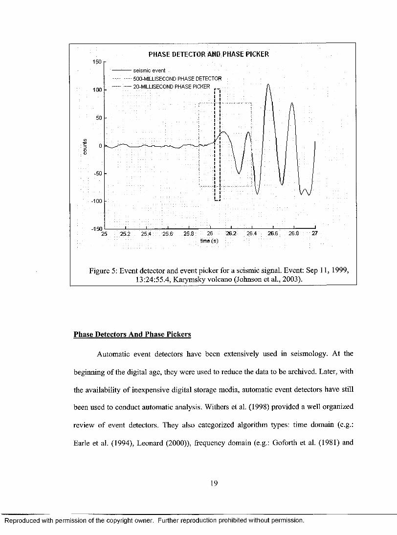
of the signal (Allen, 1982). Figure 5 shows a seismic trace and the application of a phase

detector and a phase picker (the details of seismic data acquisition for the waveforms

shown here may be found in Johnson et al. (2003)). The basic elements of a common

extraction have to include at least the arrival time, size of the event, and direction of first

motion (Allen, 1982). Depending on the computer capabilities of the system that

performs the analysis, other characteristics can be extracted such as spectral

characteristics or identification of secondary waves. In modem systems the entire digital

seismic record can be recorded which enables a complete offline analysis. In systems

where many stations are deployed and telemetry is limited an entire record is not an

option, robust automatic phase-detectors and precise phase-pickers are very important.

The system that is described in this work does not have the capabilities for continuous

storing. Therefore the implementation of a phase picker is an important component in our

analysis.

18


PHASE DETECTOR AND PHASE PICKER150

seism ic even t

500-MILLISECOND PHASE DETECTOR 20-MILLISECOND PHASE PICKER100

-50

-100

-15026.4 26.6 26.826.225.825.2 25.4 25.6

time (s)

Figure 5: Event detector and event picker for a seismic signal. Event: Sep 11, 1999, 13:24:55.4, Karymsky volcano (Johnson et al., 2003).

Phase Detectors And Phase Pickers

Automatic event detectors have been extensively used in seismology. At the

beginning of the digital age, they were used to reduce the data to be archived. Later, with

the availability of inexpensive digital storage media, automatic event detectors have still

been used to conduct automatic analysis. Withers et al. (1998) provided a well organized

review of event detectors. They also categorized algorithm types: time domain (e.g.:

Earle et al. (1994), Leonard (2000)), frequency domain (e.g.: Goforth et al. (1981) and

19


Michael et al. (1982)), particle motion (e.g.: Vidale (1986)), and adaptive window length.

Bai et al. (2000) claimed that a precise event detector has to involve multi domain

algorithms. The selection of a detector depends on the platform to be used to acquire and

process the data. Frequency domain, particle motion, and window length adaptive

detectors require the use of larger computational resources than most of the time domain

detectors. The system that is proposed by this work implements time domain event

detectors due to the limited computational capabilities of the system’s platform (40 kB

ROM and 10 kB RAM per node) and the real-time information requirements.

Time-Domain Event Detectors

Early versions of the algorithms for time domain automatic event detection are

based on comparing a current value of a signal (CY) with a predicted value (PV), which

is calculated using past states of the signal (Baer et al., 1987). An event is declared when

the ratio between CV and PV exceeds a threshold value (TH). The values that are

compared (CV and PV) can be the signal or a function of this. When a function is applied

to find the CV and PV, the function is entitled a characteristic function (CF). Examples of

characteristic functions are the absolute value, square value or standard deviation. Most

of the time-domain event detectors implement the comparison between CV and PV for a

sequence of points instead of a single point. When a sequence of points is used instead of

a single point, CV accounts for the average of a short sequence of the latest outputs of the

CF and PV for the average of a larger window. The first, short, sequence is then entitled

Short Term Average (STA) and the larger sequence Long Term Average (LTA).

20


The STA/LTA Algorithm

There are many configurations for the STA/LTA algorithms depending on the

selection of the CF and position and length of the windows. The selection of the CF is

critical in the design of a picker. Several functions have been proposed and used for

characteristic function. Allen (1982), Leonard (2000), and Withers et al. (1998) have

shown the performance of some simple functions such as the absolute value, square

value, and the standard deviation. Other groups of functions rely on complex functions

which require larger computational capabilities to be calculated (Bai et al., 2000; Earle et

al., 1994). A CF has to enhance the changes in amplitude and/or frequency of the seismic

signal. The use of the absolute value for CF was intensely used in the first automatic

pickers because it is easy to compute. The square function was also used and it has the

advantage of providing a physical meaning due to the nature of the representation of the

energy density in oscillatory systems. The absolute and square function were previously

widely used, however, their application do not permit to identify events related to

changes in the frequency content of the signal. Allen (1978) proposed a characteristic

function to enhance changes in both amplitude and frequency. Allen’s function is defined

as

CF = Y(i) + K * [ Y ( i ) - Y ( i - 1)] ( 5 )

where Y(i) is the i-th value of the signal and K is a constant that depends of the sampling

r a t e a n d n o i s e . F i g u r e 6 s h o w s a s e i s m i c e v e n t a n d t h e a p p l i c a t i o n o f d i f f e r e n t

characteristic functions for that signal. This figure shows the decoupling of a seismic

transient and background noise due to the application of different CFs. Among these

21


functions, the square value and Allen function provide better decoupling than the

absolute value function.

10

CHARACTERISTIC FUNCTIONStime (s )

30 4020 50

-50 -

200

100

sq u a re value function

0 -Allen function

60 — i—

k f .iA ---- A-.- Jj'-A .J l'-----Pj

23 23.5 24ui V

24.5 time (s )

25.5

I000

seism ic event

abso lu te value function

200

100 ■Enu

026

Figure 6: Characteristic Functions. The top trace shows an example of a seismic record, a close up of the onset of the event (seismic event) and the application of different

Characteristic Functions: absolute value, square value, and Allen function K=5. Event: _________ Sep 11, 1999, 13:51:35.0, Karymsky volcano (Johnson et al., 2003)_________

Other important parameters are the position of the STA and LTA sequences and

the process used to calculate them. Using these criteria Withers et al. (1998)

distinguished four different configurations: recursive, non-recursive, overlapped, and

delayed algorithms. Non-re cursive algorithms are based on the following equation:

22


S Tm = C F { m ) - C F ( n i - ^ , S T A ^ l ) ( 6 )Nsta

where Y(i) is the value of the signal in the i-th point, CF is the characteristic function,

and Nsta is the dimension of the STA. The same structure is applied for the calculation of

the LTA. This algorithm requires holding in memory the Nsta elements before the current

instant. The recursive algorithm is defined as:

STA(i) = C * CF(Y(i)) + (1 - C) * STA(i -1) (7)where C = 1 - e~s/T, S is the sampling period, and T is the characteristic decay time.

The second group, overlapped and delayed algorithms, accounts for the actual

position of the sequence in the time series. The delayed version features statistical

independence between sequences but the initialization requires more points than the

overlapped version. Figure 7 shows examples of the position of the STA and LTA

windows in a standard and delayed algorithm

23


POSITION OF W INDOW S FOR STA/LTA ALGORITHMS300

STALTA Standard200

100V)■£3Oo

-100seism ic event

LTA w indow

STA w indow-200

300-300STA LTA Delayed

200

100

-100

-200

-30022 24201814 16

time (s)

Figure 7: Position of windows for STA/LTA algorithms. A seismic example is analyzed with two different window configurations for an STA/LTA algorithm, Sep 11,1999,

_______________ 13:57:57.7. Karymsky volcano (Johnson et al. (2003))_______________

The third parameter in the algorithm is the length of the sequences. The STA

length needs to be short enough to be able to identify a phase arrival but large enough to

reject short change. The LTA needs to be large enough to provide an average of the

noise, and not too large that the time required after an event to calculated the LTA is too

long (Earle et al., 1994). This factor is very important because in a real time system, the

algorithm needs to finish the event and be ready for the next event. Table 1 shows some

examples of different STA and LTA length configurations.

24


STA length(s) LTA length(s) THR SENSOR REFERENCE0.01 2 2 Allen (1978)0.5 7 2 Short period Earle et al. (1994)8 30 2 Long period Earle et al. (1994)1 60 3 Mykkeltveit et al. (1984)3 24 2 Broadband Withers et al. (1998)

'able 1: Different configurations of STA/LTA algorithms

Continuous Seismic Monitoring On Volcanoes

Periods of high eruption activity are commonly accompanied by high seismic

activity. In these periods, the identification and characterization of individual events is

very difficult due to the superposition of the events. Two algorithms were developed to

identify changes in seismic activity and present a real-time approach to monitoring. The

Real-time seismic-amplitude measurement (RSAM) and the Seismic spectral-amplitude

measurements (SSAM) were developed by the USGS and used to summarize seismic

activity (Endo et al., 1991; Ewert et al., 1993). These data reduction algorithms have been

very useful during volcanic crises; their real-time nature make them useful tool for

volcano monitoring.

The RSAM calculates the average amplitude of a seismic signal over a period of

time. Different periods (1, 5, 10 minutes (Endo et al., 1991)) have been used to calculate

the RSAM for different applications. Some types of volcano activity can be monitored by

the use of this algorithm, such as increase in tremor activity. However RSAM is not able

to decipher changes in frequency. This inability can lead to misinterpretation of results.

The other approach, SSAM, involves the calculation of RSAM over band-passed pre

filtered data. This calculation can help to characterize between different kinds of activity

that in most cases refer to different physical source processes. The calculation of RSAM

25


is a straightforward algorithm in terms of computational resources. The SSAM requires

more resources and makes its implementation on a small system more challenging.

Different bandwidths have been used for SSAM analysis. These bands depend of the

analysis capabilities of the system and the desired application. If a Fourier transformation

of the signal is available a complete set of SSAM calculations is possible, which provides

very useful information (Rogers et al., 1995). Some systems are not able to perform

Fourier decomposition due to hardware and time limitations. In these systems, a SSAM

calculation can still be performed with a bandwidth that is not a single frequency but a

wide band. This approach can be performed by the use of analog or digital band-pass

filters.

Figure 8 shows an example of a signal with energy in a wide band between 0 and

10 Hz. The signal in this figure is different from pure long period (LP) events, which

usually have most of the energy in frequencies between 1 and 4 Hz. This signal has been

digitally filtered in two bandwidths, the first between 0 and 5 Hz, and the second between

5 and 10 Hz. The filtering was performed by the used of a convolution with a 49-

coefficient Finite Impulse Response (FIR) filter. These filtered signals can be used to

calculate the SSAM of the event. The result of this calculation would allow

distinguishing this event from an LP event which may produce the same RSAM. The

system that is presented by this work uses digital filtering for the calculation of the

SSAM over two frequency bands 1-5 Hz, and 5-10 Hz.

26


FREQUENCY ANALYSIS OF SIGNALS

■ seism ic event

0-5 Hz filtered signa

2000

1000

0-1000

-2000

-2000 -

• 5-10 Hz filtered signal2000

0 1 O o

15

o 10<D3O'2? 5

-2000

10 20

Figure 8: Frequency analysis of a seismic signal.A volcanic seismic signal (seismic event) is shown with its respective filtered signals (0-5 Hz filtered signal and 5-10 filtered

signal) and its spectrogram (bottom). The two filtered signals can be used for SSAM calculations. The results of this analysis can help to characterize different kinds of events.

______ Event: Sep 11,1999, 13:57:57.7, Karymsky volcano (Johnson et al. (2003))______

Digital Filters

Analog filters in modem electronic equipment have been rapidly replaced by their

digital counterparts. This migration of technology is due to the flexibility and better

performance, in most cases, of the digital filters. A digital filter is a mathematical

operation performed over a digital time series, which transforms the time series in its

time or frequency content. There are two types of digital filters: finite impulse response

27


(FIR) and infinite impulse response (HR). Three parameters can be used to describe the

performance of digital filters: filter order, stability and phase. HR filters can be

implemented, in most cases, with fewer coefficients, however a better performance can

be achieved by the FIR filters in terms of stability (always stable) and phase distortion

(linear phase always possible). There are many ways to apply a digital filter over a time

series. The theorem of convolution gives a way to apply a digital filter without the use of

a Fourier transform. This theorem establishes that a convolution in the time domain is

equivalent to the multiplication in the frequency domain and vice versa. Thus, by the

application of a convolution, a FIR filter can be efficiently used to filter a signal. This

filtered signal can be used to calculate the SSAM.

The following chapter describes an approach for an autonomous wireless seismo-

acoustic array to perform the signal processing described above. This prototype system

builds upon experience gained by the two WSNs described in the first section of this

chapter and implements very low bandwidth reports of the status of a volcano based on

the array processing without of a dedicated recorded media.

28


CHAPTER 3

DESCRIPTION OF THE WIRELESS SENSOR ARRAY

This section provides a detailed description of the wireless sensor array that is

proposed by this work. The new technology of WSN is used to implement this sensor

array. This array is intended to provide near real-time monitoring of the explosive activity

on active volcanoes. This system has been designed to perform feature extraction on

seismo-acoustic volcanic signals. This feature extraction is based on digital processing

and distributed analysis. The system is featured with array capabilities which allow a first

approach for horizontal calculation of the propagation direction of the slowness vector.

Moreover the system is able to quantify earthquake and sound intensity and calculate the

energy distribution of the activity. This chapter is divided in three main sections: 1) a

description of the hardware and software elements of the array, 2) a description of the

signal processing that is performed, and 3) the result of some lab experiments conducted

to test the performance of this system. These experiments have been designed to serve as

tests for future field installation.

Wireless Seismo-Acoustic Array: Hardware Characteristics.

The components of this system are based on the low power Moteiv Tmote Sky

wireless sensor node. These nodes feature a Texas Instruments MSP420 microcontoller,

48 kB of program memory, 10 kB of static RAM, 1024 kB of external flash memory, and

29


a 2.4-GHz Chipcon CC2420 IEEE 802.15.4 radio. TinyOS is the software platform for

programming these elements. The system consists of three types of wireless nodes: 1) a

sensor node, 2) a time synchronization node, and 3) a base station node. Figure 9 shows a

cartoon with the spatial distribution of the elements of this system.

SEISM IC AND INFRASONIC SOURCE

1-5 Km

SENSOR NODE

SENSOR NODE

50 m. separation ----- —

BASE STATION NODE

TIM E SYNCHRONIZATION NODE

50 m. separation

SENSOR NODE

Figure 9: Elements and distribution of the elements of the seismo-acoustic array proposed ________________________________by this work.________________________________

The sensor nodes

The sensor array, which is described in this chapter, includes three sensor nodes.

These nodes are in charge of the digitalization and the first stage of data analysis of a

seismic sensor and a pressure sensor. The system uses the geophone GS-1 (Geospace

30


Inc.). The GS-1 is a vertical voltage-generating ground-velocity sensor which features a 1

Hz natural frequency and a 17.78-V/(m/s) sensitivity. The pressure transducer is the

sensor DCXL01DN (Honeywell Inc) which features a 0.039-mV/Pa sensitivity. The

sampling is performed in two stages. The first includes amplification and low pass

filtering of the seismic and pressure sensors. This stage uses a custom-board conditioning

board which is described in the next subsection. The second stage in the acquisition

system involves the digitalization of the signals. The system uses the on-board mote

digitizers which feature a twelve-bit successive approximation A/D conversion. The

sampling rate of the sensor nodes has been set up to 50 Hz, in both channels. However

this sampling rate can be modified depending on the application.

Conditioning Board

The custom-designed conditioning board controls the amplification and filtering

of the analog output of the two sensors, seismic and pressure transducers. This board was

designed in conjunction with Donald Troop (Troop Instrumentation) and was constructed

to maintain low power consumption and small size, and provide low noise and high gain

capabilities. Two differential input channels can be connected to this board. A set of three

amplification options is configured by the use of jumpers; the amplifications correspond

to gains of 1, 100, and 1000. These different values for gain are appropriate for different

scenarios that can be found in the field. For instance, a gain of 1 can be useful to reject

the local noise in a locale with large signals; or in a place located very close to the source

where a event would be very intense that would saturate the channel. The other extreme,

requiring high amplification might be for placements further from the source. In the

31


amplification stage the main element in the design is the instrumentation amplifier,

AD623 (Analog Devices Inc.), which features single supply operation and rail-to-rail

output swing. The amplifier AD623 also allows the amplification of small differential

signals from sensors with low, or no, common-mode voltage. These include passive

geophones, pressure transducers, thermocouples, and others. This characteristic was

useful for the integration of the pressure transducer due to its low differential signal (less

than lOmV) and no common-mode voltage. However, the output voltage of different

seismic sensors varies considerably. For instance, the output of the 4.5 Hz GS11

geophone is 10s of millivolts, and the output of the 1-Hz GS1 seismic sensor is 100s of

millivolts. This second voltage range is unmanageable for the AD623 non-common mode

operation. Thus a 1.25 V common-voltage component has been added to the seismic

channel to allow a flexible input. The second step in the signal conditioning is the

filtering. An active 2-pole low pass filter has been implemented by the use of the low-

power, low-noise operational amplifier LM6061( National Semiconductor Inc.). Figure

10 shows the electronic diagram of amplification stage of the conditioning board (a

complete electronic diagram is included in the Appendix A.). Figure 11 shows an

example of the Tmote Sky’s 12-bit ADC and the amplification board performance. The

1-Hz signal comes from a function generator and shows three different waveforms (sine

waveform 0-3.5s, square waveform 3.5-6.5s, and triangle waveform 6.5-10s).

32


X1WCH-13-MV

M€ \ " h X*vs j—2-----VO\ i ..NC *■- — ‘X

+VO

, .T

JUM PER BLO CK JX2

ttf-lU 1A---------------------- i _

1F6P_iA_OUTup.

Figure 10: The amplification stage of the conditioning board.

EXAMPLE OF THE TMOTE SKY 12-BIT ADC1000

800

600

400

200

-200

-400

-600

-800

-1000

tim e (s)

Figure 11: Example of the Tmote Sky 12-bit ADC.

33


Time synchronization node

The time synchronization node consists on a Lassen LP GPS receiver and two

Tmote Sky motes. The first mote is connected to the serial channel and pulse per second

(PPS) line of the GPS receiver and also to the second Tmote Sky. The second mote is

connected to the GPS-receiver PPS and to the first mote. This double mote setup has been

implemented in order to simplify the management of both the acquisition of the time

from the GPS receiver and the network time synchronization. The simplification that this

configuration provides comes from the fact that the serial port of the Tmote Sky mote

shares the bus with the serial peripheral interface (SPI) bus, which communicates the

microcontroller with the radio. Thus, having a mote exclusively dedicated to

communicate with the GPS receiver allows the second mote to be in charge of the

network synchronization. In this arrangement the mote responsible for the

communication with the GPS receiver has its radio turned off. This network

synchronization mechanism requires an extensive use of the radio and implements a

variation of the Flooding Time Synchronization Protocol (FTSP) available for the Tmote

Sky platform. Figure 12 shows the elements and connections (wired and wireless) of the

time synchronization node and base node.

The base node

The base node consists in a double Tmote Sky mote setup. Similar to the time

synchronization node configuration, one mote is dedicated to the radio communication

and the other to the communication with an external device, which is in charge of the

long range communication such as radio or satellite modem (Figure 12).

34


SENSOR NODES

TIME SYNCHRONIZATION NODE

PU L S E P E R SEC O fM L IN E , CHSIVERSAL T IM E SYNCHRONIZED

ELASSEN U’ TIME MOTE 1t.I’S lfl||mrm 1 GPS cornmuhicatiohK! 1 1 l\ ! R

1TIME M 0TU 2 Time master node

A SY N C C O M MG lo b a l tim e , p o sitio n , velocity ,sateH Re ava ilab ility

SYNC CO M M year, day, second

SATELLITE BASE M<d 3 L 1 '» \> ! MO 11 :Radio Communication Event and aciivity

K M Jlu \1 0 l)l \1 message receiver.

*

ASYNC COMM. Event and activity i n formation, network status.

SYNC COMM. Event and activity information

BASE RECEIVER NODEDASHED LINES: WIRELESS CONNECTION

SOLID LINES: HARD WIRED CONNECTION

Figure 12: Elements and operation of the time synchronization and base node.

Data Analysis Description

Two kinds of data analysis are performed over the data previously digitized: a

continuous analysis and a triggered event-data processing. This data analysis is

p e r f o r m e d i n t h e s e n s o r n o d e s a n d m a n a g e d b y t h e s o f t w a r e c o m p o n e n t D a t a A n a l y s i s .

This component as well as the rest of the software elements of the array is written in the

language nesC. nesC is an efficient and robust programming language for networked

35


embedded systems (Gay et al., 2003). The complete source code for the DataAnalysis is

included in Appendix B.

The continuous analysis calculates RSAM and two SSAMs over regular intervals.

This analysis is user-configurable in total length and overlapping. The SSAM

calculations are performed by the application of two FIR filters in two different

bandwidths 0-5 Hz and 5-10Hz. Figure 13 and Figure 14 show the frequency responses

of the filters.

Frequency re sp o n se of th e 0-5Hz 50-integer coefficient low p a s s filter

a)= -50

j f -100

-150

Frequency (Hz)

x .

0)CDCD

-500

05s , -100005CO

-2 -1500CL

-2000

Frequency (Hz)

Figure 13: Frequency and phase response 0-5 Hz low pass filter

36


Frequency response of the 5-10Hz 50-integer coefficient band pass filter

CD

=5 -50

TVNcCD CJ52 -100

-150

Freq u en cy (Hz)

500

<0 uCDCD

™ -500CD

T 3

® -1000CD03

a . -1500

-2000

F req u en cy (Hz)

Figure 14: Frequency and phase response 5-10 Hz band pass filter

The information that is synthesized by this continuous analysis is collected by

each sensor node and transmitted to the base station using the message activityMsg.

Table 2 describes the size and the purpose of the elements of the activityMsg. The

structure of the message activityMsg is shown below:

typedef struct activityMsg {

uintl6_t srcAddr;

uintl6_t seqno;

uintl6_t counter;

uint32_t ini time;

uint32_t RSAM 1;

uint32_t SSAM lowl;

37


uint32_t SSAM highl;

uint32_t RSAM2;

uint32_t SSAM_low2;

uint32_t SSAM_high2;

} activityMsg ;

VARIABLE SIZE(Bytes) PURPOSEsrcAddr 2 ID of the sensor nodeSeqno 2 Sequence numbercounter 2 Number of samplesini time 4 Time of the beginning of this RSAM sequenceRSAM1 4 RSAM CHISSAM lowl 4 SSAM 0-5 Hz CHISSAM highl 4 SSAM 5-10 Hz CHIRSAM2 4 RSAM CH2SSAM low2 4 SSAM 0-5 Hz CH2SSAM high2 4 SSAM 5-10 Hz CH2

Table 2: Description of the variables of the message activityMsg

The second analysis is trigger based and is intended to extract the basic

characteristics of an event. This analysis begins with a phase detector based on a

STA/LTA algorithm. The parameters of a typical configuration for the phase detector are

shown in Table 3 (this configuration is also used in the laboratory tests in the next

section). The information that is transmitted to the base station after an event is declared

over includes: the onset and end time of the event, polarity, the last value of the STA

before the onset of the event, which is an estimation of background noise, the magnitude

and position of the maximum value in the event, and a sequence of 10 elements, which is

a decimated version of the event. Each point of the decimated version of the event is the

38


average of the signal during 6 second, this value of 6 seconds was chosen considering the

average duration of a volcanic event, which is between 50-60 seconds.

PARAMETER VALUE UNITSCHARACTERISTICFUNTION

Square value

STA LENGTH WINDOW 0.5 SLTA LENGTH 8 sTHRESHOLD 4 Ratio

Table 3: Parameters of the STA/LTA algorithm

The in form ation that is extracted by this event analysis is transmitted to the base

station using the message eventMsg. The structure of the message eventMsg is shown

below (Table 4 describes the size and the purpose of the elements of this message):

typedef struct eventMsg {

uintl6_t srcAddr;

uintl6_t seqno;

uint 16_t eventON;

uint32_t time_ini;

uint32_t tim eend;

uintl6_t polarity

uint32_t preevent_STA;

uintl6_t posMAX;

int32_t max_value;

uint32_t STAevent_ON[10];

} eventMsg;

39


VARIABLE SIZE(Bytes) PURPOSEsrcAddr; 2 ID of the sensor nodeseqno; 2 Sequence number

eventON; 2 Internal usetime ini; 4 Onset of the eventtime end; 4 End of the eventpolatiry 2 Polaritypreevent STA; 4 Last value of the STA before eventposMAX; 2 Position maximum valuemax value; 4 Maximum valueSTAevent ONI" 101; 40 Decimated version

Table 4: Description of the variables of the message eventMsg.

Laboratory Test Results

In order to test the performance of the system different experiments were carried

out in the lab. The algorithm aboard the sensor nodes that performs the RSAM and the

two SSAMs, was tested using an analog signal from a function generator. The RSAM and

SSAM algorithms were set up to 1-minute window length with 33% overlap. The output

of the generator was a monochromatic sine wave .The amplitude was kept constant and

the frequency changed in 13-minute intervals. The frequencies that were used in this test

were 2, 5, 8, and 15 Hz. These different frequencies were chosen to simulate volcano

signals. Figure 15 shows the results of this test. An important test of the system is that

even under different frequencies the value of the RSAM persists almost unaltered and the

SSAM can efficiently distinguish changes in the frequency content of the signal.

40


400

350

300

250

</>I 200oo

150

100

50

0

400

300

1 200oo100

0

RSAM AND SSAM ABOARD THE SENSOR NODE

RSAM

2 Hz 5 Hz 8 Hz 15 Hz

/

mm*.

SSAM 0-5 Hz400

300

200 1

100

0SSAM 5-10 Hz

2000 2500 3000 3500 4000 4500 5000 5500 6000 6500 7000time (s)

Figure 15: RSAM and SSAM aboard the sensor node. In this figure one of the sensor nodes applies a RSAM and two SSAMs, to a monochromatic sine wave that

__________undergoes a change in frequency through 13-minute intervals.__________

The second test includes the validation of the picking algorithm and its accuracy.

For this test the sensor nodes were colocated in a room, the picking algorithm was

applied to the infrasonic channel of the sensor nodes. The variations in pressure were

generated by the slamming of the room’s door. In this experiment all sensors experienced

41


39756429099594

4514692945245^

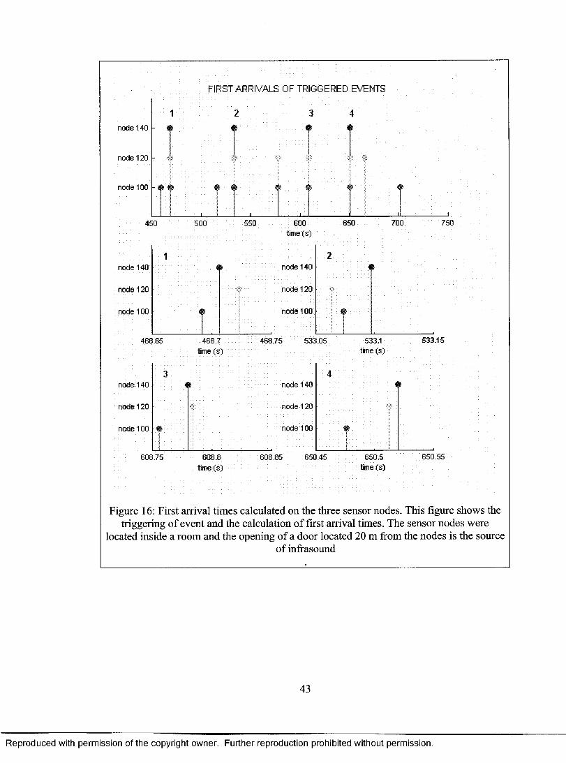
the same decompression. Figure 16 shows the results of this experiment. In this figure, a

color mark means that a sensor node identify an event. The events 1, 2, 3, and 4 are

identified by all the sensor nodes. In these triggered events the differences between the

first arrival times are within a 50 ms interval. These inaccuracies in the calculation are

related: 1) interference between the analog channels, or 2) variations in the power line

during the operation of the radio transceiver. In the proposed topology of this system, a

140 ms time lag is expected for the arrival of the infrasound wave to all the different

sensor nodes. This lag is due to the sound’s speed (331 m/s) and the 50-m separation of

the nodes. This 140 ms is still longer that our time accuracy. Thus, this system will be

able to track an air wave crossing through the array.

42


node 140 -

node 120

node 100

450

node 140

node 120

node 100

FIRST ARRIVALS OF TRIGGERED EVENTS

* *

608.75

500 550 600 time (s)

650 700

time fs) time (s)

608.8 time (s)

608.85time (s)

750

node 140node 140

node 120node 120

node 100node 100

533.15533.05 533.1468.75468.65 468.7

40

20

00

650.5 650.55650.45

Figure 16: First arrival times calculated on the three sensor nodes. This figure shows the triggering of event and the calculation of first arrival times. The sensor nodes were

located inside a room and the opening of a door located 20 m from the nodes is the sourceof infrasound

43


CHAPTER 4

CONCLUSIONS, RECOMMENDATIONS, FIELD DEPLOYMENT ANDFUTURE WORK

Conclusions and Recommendation

I have developed a wireless sensor array to conduct real-time autonomous data

analysis of seismo-acoustic signals generated by volcanic earthquakes. This project has

demonstrated the feasibility of the application of digital signal processing aboard a

wireless sensor array for monitoring volcanoes. The algorithms that have been developed

allow the application of a phase detector and a phase picker, as well as RSAM and

SSAM, which are common analysis tools for volcano seismology. The phase picker uses

a STA/LTA algorithm, which can be configured for length of the windows and the

characteristic function that is used. The calculation of RSAM was very straightforward

and its high configurability (time window and overlap) will be useful as a real-time

measurement of volcano activity. The SSAM calculation will be also useful as it can

provide a mean to distinguish different types of earthquake activity such as fluid

movement and volcano tectonic activity. This system uses the Tmote Sky sensor nodes,

which has provided an adequate platform. Its high RAM and ROM resources along with

its flexible programming language have facilitated the design of the algorithms.

44


During the course of this study some shortcomings have become apparent in

hardware and software elements. A specific hardware limitation of this system is the

small input range and low accuracy of the built-in analog-to-digital converter of the

Tmote Sky mote. Moreover, the use of just one converter and a switching mechanism

introduces noise on the channels and interference between channels. The analog to digital

conversion is also affected when the radio is receiving or transmitting information. These

hardware related problems also affect the software components. For example, the phase

picking algorithm (based on a STA/LTA algorithm) is very accurate on synthetic signals,

however when implemented on the board its effectiveness decreases due to noise on the

analog-to-digital convesion.

The computational resources of the sensor nodes also impose a limit in the types

of analysis. For example, the double 50-coefficient convolution that is used to filter data

to calculate the SSAM requires between 4-5 ms per channel to be completed, which

represents 45% of the time between conversions (50 Hz sampling rate). These operations

leave only 55% or less of the time for the other data analyses including, the time

synchronization, consecutive conversions, and networks requirements. Considering these

usage requirements, computational limits are nearly reached. Thus a double 100-

coefficient convolution, which is far from an extensive data analysis in seismology, may

be the limit of our devices in terms of computation.

45


Field deployment

The system that has been described in the previous chapter is scheduled for

deployment at Tungurahua volcano in August 2007.1 plan to install the array 3 km from

the vent together with a Freewave radio modem that will be used to relay the information

from the base station to the Tungurahua Volcano Observatory (operated by the Insituto

Geofisico, Escuela Politecnica Nacional). The topology of the array will be a 50-m

equilateral triangle with a seismo-acoustic sensor node at each vertex. The base station

and the time synchronization node will be located within the triangle (Figure 9). The

information generated by this system will include the number and timing of explosions,

polarity, length, and maximum intensity of the recorded signals, RSAM, and two SSAM

in different bandwidths. The purpose of this deployment is to test this system and

demonstrate the system’s capabilities as a robust tool for volcano monitoring and show

that its low power requirements, small size, and autonomy make the system ideal for

remote installation.

Future Work

Exciting opportunities for volcano studies are now available through WSN. The

current available hardware enables important real time data analysis. However some

limits in this analysis have also been exposed. To overcome these problems a new

generation of sensor nodes should be developed, which may integrate the existing

wireless platform with high accuracy analog to digital converters and exclusively

dedicated data analysis units. The use of 24-bit ADC has been demonstrated by previous

work (see chapter 2). Dedicated units may be in charge of extensive data analysis such as

46


frequency analysis and waveform coda analysis. Currently available technologies include

a great variety of these units, which can be as simple as single chips for filtering or

complete microcontrollers specialized in data processing. Future work should focus on

the development of low power wireless sensor arrays and networks to perform extensive

digital processing to accomplish real time location and characterization of volcanic

earthquakes.

47


REFERENCES

1. Aki, K. and Ferrazzini, V. (2000): Seismic monitoring and modeling of an

active volcano for prediction. Journal of Geophysical Research, 105(B7),

16,617-16,640.

2. Allen, R.V. (1978): Automatic earthquake recognition and timing from single

traces. Bulletin of the Seismological Society of America, 68, 1521-1532.

3. Allen, R. (1982): Automatic phase pickers: their present use and future

prospects. Bulletin of the Seismological Society of America, 72, S225-242.

4. Almendros, J., Chouet, B., Dawson, P., and Huber, C. (2002): Mapping the

sources of the seismic wave field at Kilauea volcano, Hawaii, using data

recorded on multiple seismic antennas. Bulletin of the Seismological Society

of America, 92, 2333-2351.

5. Baer, M. and Kradolfer, U. (1987): An automatic phase picker for local and

teleseismic events. Bulletin of the Seismological Society of America, 77,

1437-1445.

6. Bai, C. and Kennett, B.L. (2000): Automatic phase-detection and

identification by full use of a single three-component broadband seismogram.

Bulletin of the Seismological Society of America, 90, 187-198.

7. Buttner, R. (1998): Physics of thermohydraulic explosions. Physical Review

E, 57, 5726.

8. Buttner, R., Dellino, P., La Volpe, L., Lorenz, V., and Zimanowski, B. (2002):

Thermohydraulic explosions in phreatomagmatic eruptions as evidenced by

48


the comparison between pyroclasts and products from molten fuel coolant

interaction experiments. Journal of. Geophysical. Research, 107(B11), 227,

doi:l 0.1029/2001JB000511.

9. Cashman, K.V., Sturtevant, B., Papale, P., and Navon, O. (2000): Magmatic

fragmenation. Enciclopedia of Volcanoes, Academic Press, San-Diego, 421-

430.

10. Collombet, M., Grassoand, J. R, and Ferrazzini, V. (2003): Seismicity rate

before eruptions on piton de la Foumaise volcano: implications for eruption

dynamics. Geophysical. Research. Letters, 30(21), 2099,

doi: 10.1029/2003GL017494.

11. Del Pezzo, E., La Rocca, M., and Ibanez, J. (1997): Observations of high-

frequency scattered waves using dense arrays at Teide volcano. Bulletin of

the Seismological Society of America, 87, 1637-1647.

12. Dzurisin, D. (2003): A comprehensive approach to monitoring volcano

deformation as a window on the eruption cycle. Reviews of Geophysics,

41(1), doi: 10.1029/2001RG000107.

13. Earle, P.S. and Shearer, P.M. (1994): Characterization of global seismograms

using an automatic-picking algorithm. Bulletin of the Seismological Society

of America, 84, 366-376.

14. Endo, E.T. and Murray,T. (1991): Real-time seismic amplitude measurement

(rsam): a volcano monitoring and prediction tool. Bulletin of Volcanology, 53,

533-545.

49


15. Ewert, J., Murray, T., Lockhart, A., and Miller, C. (1993): RSAM - real-time

seismic-amplitude measurement system and SSAM - seismic spectral-

amplitude measurement system. Preventing Volcanic Catastrophe: The U.S.

International Volcano Disaster Assistance Program: Earthquakes and

Volcanoes, 24, no.6.

16. Followil, F.E., Wolford, J.K., and Candy, J.V. (1997): Advanced array

techniques for unattended ground sensor applications. Peace and Wartime

Applications and Technical Issues for Unattended Ground Sensors Orlando

FL, April 21-25,

17. Garces, M.A., McNutt, S.R., Hansenand, R.A., and Eichelberger, J.C. (2000):

Application of wave-theoretical seismoacoustic models to the interpretation of

explosion and eruption tremor signals radiated by Pavlof volcano, Alaska.

Journal of Geophysical Research, 105(B2), 3039-3058.

18. Gay, D., Levis, P., von Behren, R., Welsh, M., Brewer, E., and Culler, D.

(2003): The nesc language: a holistic approach to networked embedded

systems., In Proceedings of Programming Language Design and

Implementation (PLDI) 2003, June 2003.

19. Goforth, T. and Herrin, E. (1981): An automatic seismic signal detection

algorithm based on the Walsh transform. Bulletin of the Seismological

Society of America, 71, 1351-1360.

20. Goldstein, P., and Chouet, B. (1994): Array measurements and modeling of

sources of shallow volcanic tremor at Kilauea volcano, Hawaii. Journal of

Geophysical Research, 99(B2), 2637-2652.

50


21. Hsu, V., Kahn, J.M., and Pister, K.S.J. (1998): Wireless communications for

smart dust, URL = citeseer.ist.psu.edu/618134.html.

22. Janssen, V. (2007): Volcano deformation monitoring using GPS. Journal of

Spatial Science, 52, No.l.

23. Janssen, V., Roberts, C., Rizos, C. and Abidin, H.Z. (2001): Experiences with

a mixed-mode gps-based volcano monitoring system at Mt. Papandayan,

Indonesia, Geomatics Research Australasia, 74, 43-58.

24. Johnson, J.B., Aster, R.C., Ruiz, M.C., Malone, S.,D., McChesney, P.J., Lees,

J.M. and Kyle, P. (2003): Interpretation and utility of inffasonic records from

erupting volcanoes. Journal of Volcanology and Geothermal Research, 121,

15-63.

25. Johnson, J. and Aster, R. (2005): Relative partitioning of acoustic and seismic

energy during strombolian eruptions. Journal of Volcanology and Geothermal

Research, 148, 334-354.

26. Kahn, J., Katz, R., and Pister, K. (2000): Emerging challenges: mobile

networking for "smart dust". Journal of Communication Networks, Sept.

2000, 188-196.

27. Kushnir, A.F., Lapshin, V.M., Pinsky, V.I., and Fyen, J. (1990): Statistically

optimal event detection using small array data. Bulletin of the Seismological


28. La Rocca, M., Del Pezzo, E., Simini, M., Scarpa, R. and De Luca, G. (2001):

Array analysis of seismograms from explosive sources: evidence for surface

51


waves scattered at the main topographical features. Bulletin of the

Seismological Society of America, 91, 219-231.

29. Leonard, M. (2000): Comparison of manual and automatic onset time picking.


30. Mainwaring, A., Culler, D., Polastre, J., Szewczyk, R. and Anderson, J.

(2002): Wireless sensor networks for habitat monitoring., 88-97.

31. Maroti, M., Kusy, B., Simon, G., and Ledeczi, A. (2004): The Flooding

Synchronization Protocol., Proceedings Of the Second ACM Conference on

Embedded Networked Sensor Systems (SenSys).

32. McGetchin, T. and Chouet, B. (1979): Energy budget of the volcano

Stromboli, Italy. Geophysical research letters, 6 No.4, 317-320.

33. Michael, A.J., Gildea, S.P., and Pulli, J.J. (1982): A real-time digital seismic

event detection and recording system for network applications. Bulletin of the

Seismological Society of America, 72, 2339-2348.

34. Morrison, L.S. and Watson, R. (1961): The electronic computer and

geophysics. Geophysics, 26, 40-44.

35. Mykkeltveit, S. and Bungum, H. (1984): Processing of regional seismic events

using data from small-aperture arrays. Bulletin of the Seismological Society

of America, 74,2313-2333.

36. Metaxian, J., Lesage, P., and Dorel, J. (1997): Permanent tremor of Masaya

volcano, nicaragua: wave field analysis and source location. Journal of

Geophysical Research, 102(B10), 22,529-22,546.

52


37. Pyle, D.M. (1995): Mass and energy budgets of explosive volcanic eruptions.

Geophysical. Research. Letters, 22(5), 563-566.

38. Raghunathan, V., Ganeriwal, S., and Srivastava, M. (2006): Emerging

techniques for long lived wireless sensor networks. IEEE Communications

Magazine, April, 108-114.

39. Rogers, J.A. and Stephens, C.D. (1995): SSAM: real-time seismic spectral

amplitude measurement on a pc and its application to volcano monitoring.


40. Rost, S., and C. Thomas (2002): Array seismology: methods and applications.

Reviews of. Geophysics, 40(3), 1008.

41. Ruiz, M.C., Lees, J.M., and Johnson, J.B. (2006): Source constraints of

Tungurahua volcano explosion events. Bulletin of Volcanology, 68, 480-490.

42. Simkin, T. and Siebert, L. (2000): Earth's volcanoes and eruptions: an

overview. Enciclopedia of volcanoes. Academic Press, San-Diego, 249-261.

43. Vidale, J.E. (1986): Complex polarization analysis of particle motion. Bulletin

of the Seismological Society of America, 76, 1393-1405.

44. Wemer-Allen, G., Johnson, J., Ruiz, M., Lees, J., and Welsh, M. (2005):

Monitoring volcanic eruptions with a wireless sensor network. In Proc.

Second European Workshop on Wireless Sensor Networks, January 2005

45. Wemer-Allen, G., Lorincz, K., Johnson, J., Lees, J., and Welsh, M. (2006):

Fidelity and yield in a volcano monitoring sensor network. In Proceedings of

the 7th Conference on USENIX Symposium on Operating Systems Design

53


and Implementation - Volume 7 (Seattle, WA, November 06 - 08,2006).

USENIX Association, Berkeley, CA, 27-27.

46. Withers, M., Aster, R., and Young, C. (1999): An automated local and

regional seismic event detection and location system using waveform

correlation. Bulletin of the Seismological Society of America, 89, 657-669.

47. Withers, M., Aster, R., Young, C., Beiriger, J., Harris, M., Moore, S., and

Trujillo, J. (1998): A comparison of select trigger algorithms for automated

global seismic phase and event detection. Bulletin of the Seismological


48. Woods, A.W. (1995): The dynamics of explosive volcanic eruptions. Reviews

of Geophysics, 33, Issue 4, 495-530.

49. Zimanowski, B., Buttner, R., Lorenzand, V., and Hafele, H. (1997):

Fragmentation of basaltic melt in the course of explosive volcanism. Journal

of Geophysical Research, 102(B1), 803-814.

54


APPENDICES

55


Appendix A: Electronic Diagram Of The Conditioning Board

56


57


58


Appendix B: The “Dataanalvsis” Component Source Code

This appendix shows the source code for the component Dataanalysis. This

software was written in the language programming nesC. This component is

responsible for the application of the signal processing that is performed by this

sensor array:

* @author Omar Marcillo* @version 1.0, May 10, 2007*/

#include "DataAnalysis.h"

interface DataAnalysis {command resu ltt init();command result t add_sample(uintl6_t samplel,uintl6_t sample2);command void setTime(uint32_t time);event result t endEvent(eventMsg evl,uintl6_t typeE);event result_t contActivity(activityMsg ac);event void errorCalc(uint8_t errorType);}

59


#include "fir.h"#include "DataAnalysis.h"#include "PrintfUART.h”#include "debbugFUCT.h"

module DataAnalysisM {

provides interface DataAnalysis;uses interface LocalTime<T32khz> as LocalTime32khz;uses interface GlobalTime<T32khz> as GlobTime;

}

implementation{

// ===================== Data

uintl 6_t dataMAIN 1;intl6_t buffCHS [SIZEBUFF]; uint32_t tailCHS[SIZE_TAIL];

uintl 6_t dataMAIN2;intl6_t buffCHI[SIZE_BUFF]; uint32_t tailCF!I[SIZE TAIL];

// =======variables for suppresion of DCuintl 6_t countlNI;

uint32_t offsetsum l; uintl 6_t offauxl; uint32_t offset_sum2; uintl 6_t offaux2;

// = = = variables for data analysis uint8_t posBUFFS; uintl 6_t posTAILS; intl6_t sampsignedl;

uint8_t posBUFFI; uintl6_t posTAILI; intl6_t sampsigned2;

//===:variables for general counter uint 16_t countGEN 1; datafilt datfilteredG l;

60


uintl 6_t counterFAl; uint 16_t seqNUMES; uintl6_t seqNUMEI;

uintl 6_t count_GEN2; datafilt dat_filteredG2; uintl6_t counterFA2; uintl6_t seqNUMA;

//===variable for process on data uint8_t filFIRl; //apply the Fir filters to the data uint8_t rsams 1; //pick the first arrivals uint8_t pickFAl; //pick the first arrivals uint8_t filFIR2; //apply the Fir filters to the data uint8_t rsams2; //pick the first arrivals uint8_t pickFA2; //pick the first arrivals

uint32_t auxRSAMl; uint32_t auxSSAMLl; uint32_t auxSSAMHl;

uint8_t statusGEN;

uint32_t auxRSAM2; uint32_t auxSSAML2; uint32_t auxSSAMH2;

uint8_t statusGEN2;

// DATA FOR PICKING PROCCESS uint8_t aux_ratio; uint8_t auxcoun tev ;

uint32_t preSTAS; uint32_t preSTAI;

//===variable aux int8_t iauxl;

//===variable dataTX struct stalta inf staltaCHS; struct eventMsg eventCHS; struct activityMsg activityCHS;

struct stalta inf staltaCHI; struct eventMsg eventCHI; struct activityMsg activityCHI;

61


// = = variables for time uint32_t timeauxl;

// ==== variables for FIR int32_t v a ld sp ll; int32_t valdspl_2;//int32_t valdsp2_l;//int32_t valdsp2_2; int32_t auxlocal; uint8_t posFIR;

// ======================= Methods

uint32_t characFunc(intl6_t value); // Characteristic functionuintl 6_t abslnt(intl6_t value);void filtFIR();void pick_arrivS();void pick_arrivl();void rsamcal();

command result t DataAnalysis.init(){count_INI=0;

auxRSAMl=0;auxSSAMLl=0;auxSSAMHl=0;offset_suml=0;auxRSAM2=0;auxSSAML2=0;auxSSAMH2=0;offset_sum2=0;

filFIRl=l;pickFAl=0;rsamsl=l;

filFIR2=0;pickFA2=0;rsams2=0;

posTAILS=0;posTAILI=0;

statusGEN=0;seqNUMES=0;seqNUMEI=0;

62


seqNUMA=0; return SUCCESS;

}

inline void DCSup(uintl6_t saml,uintl6_t sam2){if((count_INI)<=(DCLENGTH-1)) { offsetsum 1 +=sam 1; offset_sum2+=sam2; sampsignedl=0; sampsigned2=0; count_INI++;}

else{offsetsum 1 +=sam 1;offaux 1 =(offset_sum 1 )/(DCLENGTH+1); offsetsum 1 -=offaux 1;sampsignedl=(saml-(offset_suml/(DCLENGTH)));

offset_sum2+=sam2;offaux2=(offset_sum2)/(DCLEN GTH+1); offset_sum2-=offaux2;sampsigned2=(sam2-(offset_sum2/(DCLENGTH)));}

}inline void dat_in_buff(){

buffCHS[posBUFFS]=sampsignedl;posBUFFS=((posBUFFS+l)%SIZE_BUFF);

buffCHI[posBUFFI]=sampsigned2;posBUFFI=(posBUFFI+1 )%SIZE_BUFF;

}intl6_t dat_out_buffI(int8_t posi){

uint8_t posOUTBUFF; if(posBUFFI>=posi) {

posOUTBUFF=posBUFFI-posi;}

else{posOUTBUFF=SIZE_BUFF+(posBUFFI-posi);}

return buffCHI[posOUTBUFF];

intl6_t dat_out_buffS(int8_t posi){ uint8_t posOUTBUFF; if(posBUFFS>:=posi) {

63


posOUTBUFF=posBUFFS-posi;}

else{posOUTBUFF=SIZE_BUFF+(posBUFFS-posi);}

return buffCHS [posOUTBUFF];

uint8_t flagS; uint8_t flagl;

task void dataANAGEN(){

DCSup(dataM AIN 1 ,dataMAIN2); dat_in_buff(); if(filFIRl)

{filtFIR();}

if(pickFAl) {pick_arrivS();

}if(pickFA2) {

pick_arrivl();}

if(rsamsl) rsamcal(); statusGEN=0;}

command void DataAnalysis.setTime(uint32_t time){timeauxl=time;}

command result t DataAnalysis.add_sample(uintl6_t datal,uintl6_t data2){if(statusGEN==0) {

statusGEN=l; dataM AIN 1 =data 1; dataMAIN2=data2;

if(post dataANAGEN()) {return SUCCESS;} else {return FAIL;}}

else {statusGEN=0;

signal DataAnalysis.errorCalc(l);

64


return FAIL;}}

uint32_t characFunc(intl6_t value) {return ((uint32_t)(((int32_t)value)*(int32_t)value));}

uintl 6_t abslnt(intl6_t value) { if((value & 0x8000)1=0) {

return((uintl6_t)(((~value) & 0x7FFF)+l));}

else{return (uintl6_t)value;}

}inline void rsamcal(){

auxRS AM 1 +=abslnt(sampsigned 1); auxSSAMLl+=absInt(dat_filteredGl.datalowfilt); auxS S AMH1 +=abslnt(dat_fi IteredG 1 .datahighfilt); auxRS AM2+=absInt(sampsigned2); auxSSAML2+=absInt(dat_filteredG2.datalowfilt); auxSSAMH2+=absInt(dat_filteredG2.datahighfilt); activityCHS. counter++;if(activityCHS.counter==(SIZE_RSAM-OVRL_PERC)){

activityCHS. ini_time= call GlobTime.get(); activityCHS. seqno=seqNUM A; seqNUMA=seqNUMA+l; activityCHS.RSAMl =auxRSAMl; activityCHS.SSAMlowl =auxSSAMLl; activityCHS.SSAM_highl=auxSSAMH 1; activityCHS.RSAM2 =auxRSAM2; activityCHS. SSAM_low2 =auxSSAML2; activityCHS.SSAM_high2=auxSSAMH2; auxRS AMI = 0; auxSSAMLl = 0; auxSSAMHl = 0; auxRSAM2 =0; auxSSAML2 = 0; auxSSAMH2 = 0;}

if(activityCHS.counter==(SIZE_RSAM)){ activityCHS. RSAM 1 +=auxRS AM 1; activityCHS. S S A M low 1 +=auxS S AML 1; activityCHS. SS AM_high 1 +=auxS S AMH 1;

65


activityCHS.RSAM2+=auxRSAM2; activity CHS. S S AM_low2+=auxS S AML2; activityCHS. S S AM_high2+=auxS S AMH2;

activityCHS. counter=0 V RLPERC; signal DataAnalysis. cont Activity(activityCHS); }

void filtFIR(){//FIR filter with NUM COEF coefficients valdsp 1 1 =0; valdsp 1 2=0;

for(iauxl=0;iauxl<NUM_COEF;iauxl++){ if((posBUFFS-iauxl)>=0) {

posFIR=posBUFFS-iauxl;}

else{posFIR=NUM_COEF+(posBUFFS-iauxl); //this must be 51 }

auxlocal=(int32_t)buffCHS[posFIR]; valdsp 1 1 +=(auxlocal)*((int32_t)FIR5 [iauxl]); valdsp l_2+=(auxlocal)*((int32_t)FIRl 0[iauxl]); //auxlocal=(int32_t)buffCHI[posFIR];//valdsp2_ 1 +=(auxlocal) *FIR5 [iauxl]; //valdsp2_2+=(auxlocal)*FIRl 0[iauxl];

}datfilteredG 1. datalowfilt=(int 16_t)(valdsp 1_1/10000); dat_filteredGl.datahighfilt=(intl6_t)(valdspl_2/10000);}

inline void pick_arrivS() { uint32_t LTAaux; uintl6_t posintTAIL; staltaCHS. counter++; if(staltaCHS.counter==l) {

staltaCHS.LTA_shift=0; staltaCH S. S T A_value=0; staltaCHS.LTA_value=0;}

if(((staltaCHS.counter)%SIZE_STA)== 1) {if(eventCHS. eventON==0) {preST AS=staltaCHS. ST A value;} staltaCHS.ST A_value=0;

66


staltaCHS.STA_value+=characFunc(sampsignedl);

if(((staltaCHS. counter)%SIZE_ST A)==0) { if(eventCHS.eventON==0) {

staltaCH S. LT A_value+=staltaCHS. S T A value;tailCHS[posTAILS]=staltaCHS.STA_value;posTAILS=(posTAILS+l)%SIZE_TAIL;}

else{

if((staltaCHS. ST A_value<=preSTAS) 11 ((eventCHS .eventON)>=M AXIM UNE VEN T_L)){

eventCHS. eventON=0; staltaCHS. counter=0;signal DataAnalysis.endEvent(eventCHS,l); //include a parameter to tell

if the event has been cut off} //or the TH was reached

else{if((eventCHS.eventON)<MAXIMUN_EVENT_L){

eventCHS. STAevent_ON[eventCHS.eventON/15]+=staltaCHS.STA_value; eventCHS.eventON+=l;}

staltaCHS. counter=0;}

}}

if(staltaCHS. counter==(SIZE_LT A+SIZEST A)) { LTAaux=staltaCHS.LTA_value-staltaCHS.STA_value; //LTA with LTA SIZE

lengthstaltaCHS.counter=(SIZE_LTA); if(posTAILS>=(SIZE_RATIO_S_L_TA+l)) { posintTAIL=posTAILS-(SIZE_RATIO_S_L_TA+l);}

else {posintTAIL=(uintl6_t)(SIZE_TAIL+(posTAILS-

(SIZE_RATIO_S_L_TA+1)));}staltaCHS .LT A_value-=tailCHS [posintT AIL];

staltaCHS .ratio=(((staltaCHS. ST A value* SIZE_RATIO_S_L_T A) * 10)/LT Aaux); //printfUART("R_S %i\n ",(uintl6_t)staltaCHS.ratio);

if(staltaCHS.ratio>THRESHOLD_EVENT){ printfUART("PS E\t","");

67


aux_count_ev=0;// TWO CONSECUTIVES POINTS over the TH TRIGGER

AN EVENTfor(iauxl=(SIZE_STA+SIZE_STA/2);iauxl>=0;iauxl—){

// the points are going backwards, the most recent first /* this was incorrect the idea is to te4st first the last point in buffer first*/ aux_ratio=(10*characFunc(dat_out_buffS(iauxl))*SIZE_LTA)/LTAaux; if( aux ratio > THRESHOLD EVENT) {

aux_count_ev++; if(aux_count_ev >= 5){eventCHS ,posINI=iauxl; iauxl=-l;}

}else{ aux_count_ev=0;}}

if(aux count ev < 5){ printfUART("FS EV',"");}

else{printfUART("TS EV',""); flagS=l;eventCHS.eventON= 1; eventCHS ,preevent_ST A=preST AS;eventCHS .tim eini = timeauxl-eventCHS.posINI*(32768L/100); for(iauxl=0;iauxl<SIZE_STA;iauxl++){

eventCHS. ST Aevent_ON[iauxl]=0;}

eventCHS. seqno=seqNUMES; seqNUMES=seqNUMES+1;/*

for(iauxl=(SIZE_STA+SIZE_STA/2);iauxl>=0;iauxl—){ if(dat_out_buffS(iauxl)>0) { printfU ART(" %i\t" ,dat_out_buffS(iauxl));} else{printfU ART("-%i\t",0-dat_out_buffS(iauxl));}}

printfU ART("\n",'"');* /staltaCHS.counter=0;//signal DataAnalysis.startEvent(8);}

68


else {//printfUART("NS E\n",""); }

}}

inline void pick_arrivl() { uint32_t LTAaux; uintl6_t posintTAIL; staltaCHI. counter++; if(staltaCHI.counter==l) {

staltaCHI.LTA_shift=0; staltaCHI. ST A_value=0; staltaCHI. LT A_value=0;}

if(((staltaCHI.counter)%SIZE_STA)== 1) {if(eventCHI. eventON==0) {preST AI=staltaCHI. ST A value;} staltaCHI.STA_value=0;}

staltaCHI.STA_value+=characFunc(sampsigned2); if(((staltaCHI.counter)%SIZE_STA)==0){

if(eventCHI.eventON==0) {staltaCHI.LTA_value+=staltaCHI.STA_value; tailCHI[posTAILI]=staltaCHI.STA_value; posT AILI=(posTAILI+1 )%SIZE_TAIL;}

else{

if((staltaCHLSTA_value<=preSTAI)||((eventCHI.eventON)>=MAXIMUN_EVENT_L)){

printfUART("END EVENT","");//eventCH.timeend = timeaux; e ventCHI. e ventON=0; staltaCHI.counter=0;signal DataAnalysis.endEvent(eventCHI,2); //include a parameter to tell if

the event has been cut off} //or the TH was reached

else{if((eventCHI.eventON)<MAXIMUN_EVENT_L){

//eventCHI. ST Aevent_ON[eventCHI. eventON/15 ]+=staltaCHI. ST A value; eventCHI.eventON+= 1;}

stal taC HI. counter=0;}

69


}if(staltaCHI.counter==(SIZE_LTA+SIZE_STA)){

LTAaux=staltaCHI.LTA_value-staltaCHLSTA_value; //LTA with LTA SIZElength

staltaCHI.counter=(SIZE_LTA); if(posTAILI>=(SIZE_RATIO_S_L_TA+1)) {

posintTAIL=posTAILI-(SIZE_RATIO_S_L_TA+l);}

else{posintTAIL=(uintl6_t)(SIZE_TAIL+(posTAILI-

(SIZE_RATIO_S_L_TA+l)));}

staltaCHI.LTA_value-=tailCHI[posintTAIL];

staltaCHI.ratio=(((staltaCHI.STA_value*SIZE_RATIO_SL_TA)*10)/LTAaux); //printfU ART("R_I %i \n",(uintl6_t)staltaCHI.ratio); if(staltaCHI.ratio>THRESHOLD_EVENT){

printfU ART("PI_E\t'7M’); a u x c o u n t e v=0;

// TWO CONSECUTIVES POINTS over the TH TRIGGERAN EVENT

for(iauxl=(SIZE_STA+SIZE_STA/2);iauxl>=0;iauxl—){// the points are going backwards, the most recent first aux_ratio=(10*characFunc(dat_out_buffI(iauxl))*SIZE_LTA)/LTAaux; if( aux_ratio > THRESHOLD_EVENT){

aux_count_ev++; if(aux_count_ev >= 2){

eventCHI.posINI=iauxl; iauxl=-l;}

}else{ aux_count_ev=0;}}

printfU ART (" count %i\n" ,aux_count_ev);// aux_count_ev=0; if(aux_count_ev < 2){

printfU ART("FI E\n","");}

else{printfUART("TI E\n",”");

flagl=l; eventCHI.eventON= 1; eventCHI.preevent_STA=preSTAI; eventCHI.timeini = 0;//timeaux; eventCHI.posINI=iauxl;

70


eventCHI.seqno=seqNUMEI; seqNUMEI=seqNUMEI+l; for(iauxl=0;iauxl<SIZE_ST A;iauxl++) {

//eventCHI.STAevent_ON[iauxl]=0;}

staltaCHI. counter=0; printfU ART("TI End\n","");}

}

71


digital seismo-acoustic signal processing aboard a

Documents