digital workbook for gra 6035 mathematics - … · digital workbook for gra 6035 mathematics...
TRANSCRIPT
Eivind Eriksen
Digital Workbook forGRA 6035 Mathematics
November 7, 2017
BI Norwegian Business School

Contents
Part I Lectures in GRA6035 Mathematics
1 Linear Systems and Gaussian Elimination . . . . . . . . . . . . . . . . . . . . . . . . 31.1 Main concepts . . . . . . . . . . . . . . . . . . . . . . . . . . . . . . . . . . . . . . . . . . . . . 31.2 Problems . . . . . . . . . . . . . . . . . . . . . . . . . . . . . . . . . . . . . . . . . . . . . . . . . 41.3 Solutions . . . . . . . . . . . . . . . . . . . . . . . . . . . . . . . . . . . . . . . . . . . . . . . . . 7
2 Matrices and Matrix Algebra . . . . . . . . . . . . . . . . . . . . . . . . . . . . . . . . . . . . 152.1 Main concepts . . . . . . . . . . . . . . . . . . . . . . . . . . . . . . . . . . . . . . . . . . . . . 152.2 Problems . . . . . . . . . . . . . . . . . . . . . . . . . . . . . . . . . . . . . . . . . . . . . . . . . 162.3 Solutions . . . . . . . . . . . . . . . . . . . . . . . . . . . . . . . . . . . . . . . . . . . . . . . . . 22
3 Vectors and Linear Independence . . . . . . . . . . . . . . . . . . . . . . . . . . . . . . . . 313.1 Main concepts . . . . . . . . . . . . . . . . . . . . . . . . . . . . . . . . . . . . . . . . . . . . . 313.2 Problems . . . . . . . . . . . . . . . . . . . . . . . . . . . . . . . . . . . . . . . . . . . . . . . . . 323.3 Solutions . . . . . . . . . . . . . . . . . . . . . . . . . . . . . . . . . . . . . . . . . . . . . . . . . 34
4 Eigenvalues and Diagonalization . . . . . . . . . . . . . . . . . . . . . . . . . . . . . . . . . 414.1 Main concepts . . . . . . . . . . . . . . . . . . . . . . . . . . . . . . . . . . . . . . . . . . . . . 414.2 Problems . . . . . . . . . . . . . . . . . . . . . . . . . . . . . . . . . . . . . . . . . . . . . . . . . 424.3 Advanced Matrix Problems . . . . . . . . . . . . . . . . . . . . . . . . . . . . . . . . . . 444.4 Solutions . . . . . . . . . . . . . . . . . . . . . . . . . . . . . . . . . . . . . . . . . . . . . . . . . 45
5 Quadratic Forms and Definiteness . . . . . . . . . . . . . . . . . . . . . . . . . . . . . . . 555.1 Main concepts . . . . . . . . . . . . . . . . . . . . . . . . . . . . . . . . . . . . . . . . . . . . . 555.2 Problems . . . . . . . . . . . . . . . . . . . . . . . . . . . . . . . . . . . . . . . . . . . . . . . . . 565.3 Solutions . . . . . . . . . . . . . . . . . . . . . . . . . . . . . . . . . . . . . . . . . . . . . . . . . 60
6 Unconstrained Optimization . . . . . . . . . . . . . . . . . . . . . . . . . . . . . . . . . . . . 696.1 Main concepts . . . . . . . . . . . . . . . . . . . . . . . . . . . . . . . . . . . . . . . . . . . . . 696.2 Problems . . . . . . . . . . . . . . . . . . . . . . . . . . . . . . . . . . . . . . . . . . . . . . . . . 706.3 Solutions . . . . . . . . . . . . . . . . . . . . . . . . . . . . . . . . . . . . . . . . . . . . . . . . . 73
v
vi Contents
7 Constrained Optimization and First Order Conditions . . . . . . . . . . . . . 857.1 Main concepts . . . . . . . . . . . . . . . . . . . . . . . . . . . . . . . . . . . . . . . . . . . . . 857.2 Problems . . . . . . . . . . . . . . . . . . . . . . . . . . . . . . . . . . . . . . . . . . . . . . . . . 877.3 Solutions . . . . . . . . . . . . . . . . . . . . . . . . . . . . . . . . . . . . . . . . . . . . . . . . . 88
8 Constrained Optimization and Second Order Conditions . . . . . . . . . . . 958.1 Main concepts . . . . . . . . . . . . . . . . . . . . . . . . . . . . . . . . . . . . . . . . . . . . . 958.2 Problems . . . . . . . . . . . . . . . . . . . . . . . . . . . . . . . . . . . . . . . . . . . . . . . . . 968.3 Solutions . . . . . . . . . . . . . . . . . . . . . . . . . . . . . . . . . . . . . . . . . . . . . . . . . 98
9 Envelope Theorems and Bordered Hessians . . . . . . . . . . . . . . . . . . . . . . . 1059.1 Main concepts . . . . . . . . . . . . . . . . . . . . . . . . . . . . . . . . . . . . . . . . . . . . . 1059.2 Problems . . . . . . . . . . . . . . . . . . . . . . . . . . . . . . . . . . . . . . . . . . . . . . . . . 1069.3 Advanced Optimization Problems . . . . . . . . . . . . . . . . . . . . . . . . . . . . . 1089.4 Solutions . . . . . . . . . . . . . . . . . . . . . . . . . . . . . . . . . . . . . . . . . . . . . . . . . 109
10 First Order Differential Equations . . . . . . . . . . . . . . . . . . . . . . . . . . . . . . . 12510.1 Main concepts . . . . . . . . . . . . . . . . . . . . . . . . . . . . . . . . . . . . . . . . . . . . . 12510.2 Problems . . . . . . . . . . . . . . . . . . . . . . . . . . . . . . . . . . . . . . . . . . . . . . . . . 12610.3 Problems in Excel . . . . . . . . . . . . . . . . . . . . . . . . . . . . . . . . . . . . . . . . . . 12810.4 Solutions . . . . . . . . . . . . . . . . . . . . . . . . . . . . . . . . . . . . . . . . . . . . . . . . . 129
11 Second Order Differential Equations . . . . . . . . . . . . . . . . . . . . . . . . . . . . . 13711.1 Main concepts . . . . . . . . . . . . . . . . . . . . . . . . . . . . . . . . . . . . . . . . . . . . . 13711.2 Problems . . . . . . . . . . . . . . . . . . . . . . . . . . . . . . . . . . . . . . . . . . . . . . . . . 13811.3 Problems in Excel . . . . . . . . . . . . . . . . . . . . . . . . . . . . . . . . . . . . . . . . . . 14011.4 Solutions . . . . . . . . . . . . . . . . . . . . . . . . . . . . . . . . . . . . . . . . . . . . . . . . . 141
12 Difference Equations . . . . . . . . . . . . . . . . . . . . . . . . . . . . . . . . . . . . . . . . . . . 15112.1 Main concepts . . . . . . . . . . . . . . . . . . . . . . . . . . . . . . . . . . . . . . . . . . . . . 15112.2 Problems . . . . . . . . . . . . . . . . . . . . . . . . . . . . . . . . . . . . . . . . . . . . . . . . . 15312.3 Solutions . . . . . . . . . . . . . . . . . . . . . . . . . . . . . . . . . . . . . . . . . . . . . . . . . 154
Part II Exams in GRA6035 Mathematics
Part ILectures in GRA6035 Mathematics

Contents Next: Lecture 2
Lecture 1Linear Systems and Gaussian Elimination
1.1 Main concepts
An m×n linear system in the variables x1,x2, . . . ,xn is a system of m linear equationsin these variables, and can in general be written as
a11x1 + a12x2 + . . . + a1nxn = b1a21x1 + a22x2 + . . . + a2nxn = b2
......
......
am1x1 + am2x2 + . . . + amnxn = bm
A more compact notation is the matrix form Ax = b using the coefficient matrixA, and an even more compact notation is the augmented matrix A, where
A =
a11 a12 . . . a1na21 a22 . . . a2n
......
. . ....
am1 am2 . . . amn
, b =
b1b2...
bm
and A =
a11 a12 . . . a1n b1a21 a22 . . . a2n b2
......
. . ....
...am1 am2 . . . amn bm
A solution of this linear system is an n-couple of numbers (s1,s2, . . . ,sn) such thatx1 = s1, x2 = s2, . . . ,xn = sn solves all m equations simultaneously.
Lemma 1.1. Any linear system has either no solutions (inconsistent), one uniquesolution (consistent) or infinitely many solutions (consistent).
Gaussian elimination is an efficient algorithm that can be used to solve any linearsystem. We use elementary row operations on the augmented matrix of the systemuntil we reach an echelon form of the matrix, transform it back to a linear systemand solve it by back substitution. The following operations are called elementaryrow operations:
Problems Lecture 1 Solutions
4 1 Linear Systems and Gaussian Elimination
1. To add a multiple of one row to another row2. To interchange two rows3. To multiply a row with a nonzero constant
In any non-zero row, the leading coefficient is the first (or leftmost) non-zero entry.A matrix is in echelon form if the following conditions hold:
• All rows of zeros appear below non-zero rows.• Each leading coefficient appears further to the right than the leading coefficients
in the rows above.
A pivot is a leading coefficient in an echelon form, and the pivot positions of amatrix are the positions where there are pivots in the echelon form of the matrix.Back substitution is the process of solving the equations for the variables in thepivot positions (called basic variables), starting from the last non-zero equationand continuing the process in reverse order. The non-basic variables are called freevariables.
Gauss-Jordan elimination is variation, where we continue with elementary rowoperations until we reach a reduced echelon form. A matrix is in reduced echelonform if it is in echelon form, and the following additional condtions are satisfied:
• Each leading coefficient is 1• All other entries in columns with leading coefficients are 0
Gauss-Jordan elimination can be convenient for linear systems with infinitely manysolutions. Gaussian elimination is more efficient for large linear systems.
Lemma 1.2. Any matrix can be transformed into an echelon form, and also into areduced echelon form, using elementary row operations. The reduced echelon formis unique. In general, an echelon form is not unique, but its pivot positions are.
The rank of a matrix A, written rkA, is defined as the number of pivot positionsin A. It can be computed by finding an echelon form of A and counting the pivots.
Lemma 1.3. An m× n linear system is consistent if rkA = rk A, and inconsistentotherwise. If the linear system is consistent, the number of free variables is given byn− rkA.
1.2 Problems
1.1. Write down the coefficient matrix and the augmented matrix of the followinglinear systems:
a)2x + 5y = 63x − 7y = 4 b)
x + y − z = 0x − y + z = 2x − 2y + 4z = 3
1.2 Problems 5
1.2. Write down the linear system in the variables x,y,z with augmented matrix1 2 0 42 −3 1 07 4 1 3
1.3. Use substitution to solve the linear system
x + y + z = 1x − y + z = 4x + 2y + 4z = 7
1.4. For what values of h does the following linear system have solutions?
x + y + z = 1x − y + z = 4x + 2y + z = h
1.5. Solve the following linear systems by Gaussian elimination:
a)x + y + z = 1x − y + z = 4x + 2y + 4z = 7
b)2x + 2y − z = 2
x + y + z = −22x + 4y − 3z = 0
1.6. Solve the following linear system by Gauss-Jordan elimination:
x + y + z = 1x − y + z = 4x + 2y + 4z = 7
1.7. Solve the following linear systems by Gaussian elimination:
a)−4x + 6y + 4z = 4
2x − y + z = 1 b)6x + y = 73x + y = 4−6x − 2y = 1
1.8. Discuss the number of solutions of the linear system
x + 2y + 3z = 1−x + ay − 21z = 23x + 7y + az = b
for all values of the parameters a and b.
1.9. Find the pivot positions of the following matrix: 1 3 4 1 73 2 1 0 7−1 3 2 4 9
6 1 Linear Systems and Gaussian Elimination
1.10. Show that the following linear system has infinitely many solutions, and de-termine the number of degrees of freedom:
x + 6y − 7z + 3w = 1x + 9y − 6z + 4w = 2x + 3y − 8z + 4w = 5
Find free variables and express the basic variables in terms of the free ones.
1.11. Solve the following linear systems by substitution and by Gaussian elimina-tion:
a)x − 3y + 6z = −1
2x − 5y + 10z = 03x − 8y + 17z = 1
b)x + y + z = 0
12x + 2y − 3z = 53x + 4y + z = −4
1.12. Find the rank of the following matrices:
a)(
1 28 16
)b)
(1 3 42 0 1
)c)
1 2 −1 32 4 −4 7−1 −2 −1 −2
1.13. Find the rank of the following matrices:
(a)
1 3 0 02 4 0 −11 −1 2 2
b)
2 1 3 7−1 4 3 13 2 5 11
c)
1 −2 −1 12 1 1 2−1 1 −1 −3−2 −5 −2 0
1.14. Prove that any 4×6 homogeneous linear system has non-trivial solutions.
1.15. Discuss the ranks of the coefficient matrix A and the augmented matrix A ofthe linear system
x1 + x2 + x3 = 2q2x1 − 3x2 + 2x3 = 4q3x1 − 2x2 + px3 = q
for all values of p and q. Use this to determine the number of solutions of the linearsystem for all values of p and q.
1.16. Midterm Exam in GRA6035 on 24/09/2010, Problem 3Compute the rank of the matrix
A =
2 5 −3 −4 84 7 −4 −3 96 9 −5 −2 4
1.17. Mock Midterm Exam in GRA6035 on 09/2010, Problem 3Compute the rank of the matrix
1.3 Solutions 7
A =
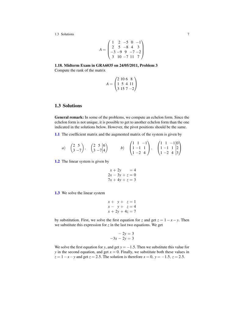
1 2 −5 0 −12 5 −8 4 3−3 −9 9 −7 −23 10 −7 11 7
1.18. Midterm Exam in GRA6035 on 24/05/2011, Problem 3Compute the rank of the matrix
A =
2 10 6 81 5 4 113 15 7 −2
1.3 Solutions
General remark: In some of the problems, we compute an echelon form. Since theechelon form is not unique, it is possible to get to another echelon form than the oneindicated in the solutions below. However, the pivot positions should be the same.
1.1 The coefficient matrix and the augmented matrix of the system is given by
a)(
2 53 −7
),
(2 5 63 −7 4
)b)
1 1 −11 −1 11 −2 4
,
1 1 −1 01 −1 1 21 −2 4 3
1.2 The linear system is given by
x + 2y = 42x − 3y + z = 07x + 4y + z = 3
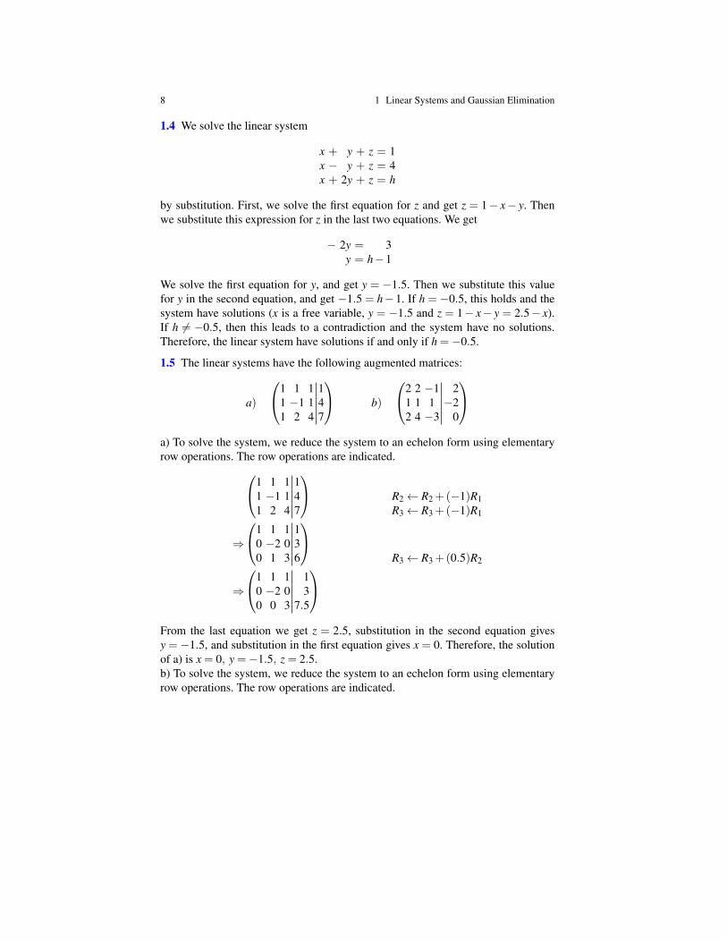
1.3 We solve the linear system
x + y + z = 1x − y + z = 4x + 2y + 4z = 7
by substitution. First, we solve the first equation for z and get z = 1− x− y. Thenwe substitute this expression for z in the last two equations. We get
− 2y = 3−3x − 2y = 3
We solve the first equation for y, and get y =−1.5. Then we substitute this value fory in the second equation, and get x = 0. Finally, we substitute both these values inz = 1− x− y and get z = 2.5. The solution is therefore x = 0, y =−1.5, z = 2.5.
8 1 Linear Systems and Gaussian Elimination
1.4 We solve the linear system
x + y + z = 1x − y + z = 4x + 2y + z = h
by substitution. First, we solve the first equation for z and get z = 1− x− y. Thenwe substitute this expression for z in the last two equations. We get
− 2y = 3y = h−1
We solve the first equation for y, and get y = −1.5. Then we substitute this valuefor y in the second equation, and get −1.5 = h−1. If h = −0.5, this holds and thesystem have solutions (x is a free variable, y = −1.5 and z = 1− x− y = 2.5− x).If h 6= −0.5, then this leads to a contradiction and the system have no solutions.Therefore, the linear system have solutions if and only if h =−0.5.
1.5 The linear systems have the following augmented matrices:
a)
1 1 1 11 −1 1 41 2 4 7
b)
2 2 −1 21 1 1 −22 4 −3 0
a) To solve the system, we reduce the system to an echelon form using elementaryrow operations. The row operations are indicated.1 1 1 1
1 −1 1 41 2 4 7
R2← R2 +(−1)R1R3← R3 +(−1)R1
⇒
1 1 1 10 −2 0 30 1 3 6
R3← R3 +(0.5)R2
⇒
1 1 1 10 −2 0 30 0 3 7.5
From the last equation we get z = 2.5, substitution in the second equation givesy = −1.5, and substitution in the first equation gives x = 0. Therefore, the solutionof a) is x = 0, y =−1.5, z = 2.5.b) To solve the system, we reduce the system to an echelon form using elementaryrow operations. The row operations are indicated.
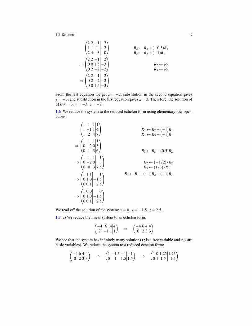
1.3 Solutions 92 2 −1 21 1 1 −22 4 −3 0
R2← R2 +(−0.5)R1R3← R3 +(−1)R1
⇒
2 2 −1 20 0 1.5 −30 2 −2 −2
R2← R3R3← R2
⇒
2 2 −1 20 2 −2 −20 0 1.5 −3
From the last equation we get z = −2, substitution in the second equation givesy =−3, and substitution in the first equation gives x = 3. Therefore, the solution ofb) is x = 3, y =−3, z =−2.
1.6 We reduce the system to the reduced echelon form using elementary row oper-ations: 1 1 1 1
1 −1 1 41 2 4 7
R2← R2 +(−1)R1R3← R3 +(−1)R1
⇒
1 1 1 10 −2 0 30 1 3 6
R3← R3 +(0.5)R2
⇒
1 1 1 10 −2 0 30 0 3 7.5
R2← (−1/2) ·R2R3← (1/3) ·R3
⇒
1 1 1 10 1 0 −1.50 0 1 2.5
R1← R1 +(−1)R2 +(−1)R3
⇒
1 0 0 00 1 0 −1.50 0 1 2.5
We read off the solution of the system: x = 0, y =−1.5, z = 2.5.
1.7 a) We reduce the linear system to an echelon form:(−4 6 4 42 −1 1 1
)⇒
(−4 6 4 40 2 3 3
)We see that the system has infinitely many solutions (z is a free variable and x,y arebasic variables). We reduce the system to a reduced echelon form:(
−4 6 4 40 2 3 3
)⇒
(1 −1.5 −1 −10 1 1.5 1.5
)⇒
(1 0 1.25 1.250 1 1.5 1.5
)
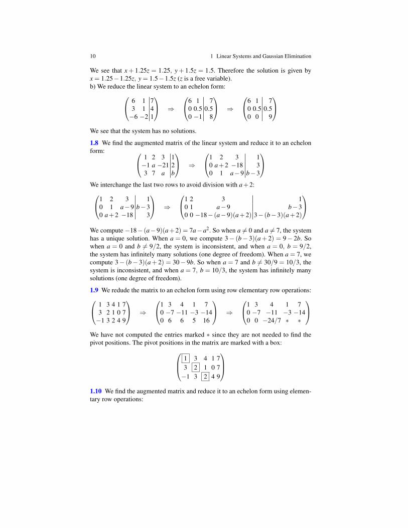
10 1 Linear Systems and Gaussian Elimination
We see that x+ 1.25z = 1.25, y+ 1.5z = 1.5. Therefore the solution is given byx = 1.25−1.25z, y = 1.5−1.5z (z is a free variable).b) We reduce the linear system to an echelon form: 6 1 7
3 1 4−6 −2 1
⇒
6 1 70 0.5 0.50 −1 8
⇒
6 1 70 0.5 0.50 0 9
We see that the system has no solutions.
1.8 We find the augmented matrix of the linear system and reduce it to an echelonform: 1 2 3 1
−1 a −21 23 7 a b
⇒
1 2 3 10 a+2 −18 30 1 a−9 b−3
We interchange the last two rows to avoid division with a+2:1 2 3 1
0 1 a−9 b−30 a+2 −18 3
⇒
1 2 3 10 1 a−9 b−30 0 −18− (a−9)(a+2) 3− (b−3)(a+2)
We compute −18− (a−9)(a+2) = 7a−a2. So when a 6= 0 and a 6= 7, the systemhas a unique solution. When a = 0, we compute 3− (b− 3)(a+ 2) = 9− 2b. Sowhen a = 0 and b 6= 9/2, the system is inconsistent, and when a = 0, b = 9/2,the system has infinitely many solutions (one degree of freedom). When a = 7, wecompute 3− (b− 3)(a+ 2) = 30− 9b. So when a = 7 and b 6= 30/9 = 10/3, thesystem is inconsistent, and when a = 7, b = 10/3, the system has infinitely manysolutions (one degree of freedom).
1.9 We redude the matrix to an echelon form using row elementary row operations: 1 3 4 1 73 2 1 0 7−1 3 2 4 9
⇒
1 3 4 1 70 −7 −11 −3 −140 6 6 5 16
⇒
1 3 4 1 70 −7 −11 −3 −140 0 −24/7 ∗ ∗
We have not computed the entries marked ∗ since they are not needed to find thepivot positions. The pivot positions in the matrix are marked with a box: 1 3 4 1 7
3 2 1 0 7−1 3 2 4 9
1.10 We find the augmented matrix and reduce it to an echelon form using elemen-tary row operations:
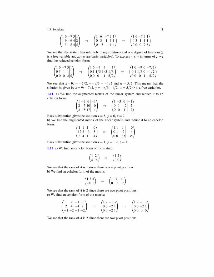
1.3 Solutions 111 6 −7 3 11 9 −6 4 21 3 −8 4 5
⇒
1 6 −7 3 10 3 1 1 10 −3 −1 1 4
⇒
1 6 −7 3 10 3 1 1 10 0 0 2 5
We see that the system has infinitely many solutions and one degree of freedom (zis a free variable and x,y,w are basic variables). To express x,y,w in terms of z, wefind the reduced echelon form:1 6 −7 3 1
0 3 1 1 10 0 0 2 5
⇒
1 6 −7 3 10 1 1/3 1/3 1/30 0 0 1 5/2
⇒
1 0 −9 0 −7/20 1 1/3 0 −1/20 0 0 1 5/2
We see that x− 9z = −7/2, y + z/3 = −1/2 and w = 5/2. This means that thesolution is given by x = 9z−7/2, y =−z/3−1/2, w = 5/2 (z is a free variable).
1.11 a) We find the augmented matrix of the linear system and reduce it to anechelon form: 1 −3 6 −1
2 −5 10 03 −8 17 1
⇒
1 −3 6 −10 1 −2 20 0 1 2
Back substitution gives the solution x = 5, y = 6, z = 2.b) We find the augmented matrix of the linear system and reduce it to an echelonform: 1 1 1 0
12 2 −3 53 4 1 −4
⇒
1 1 1 00 1 −2 −40 0 −35 −35
Back substitution gives the solution x = 1, y =−2, z = 1.
1.12 a) We find an echelon form of the matrix:(1 28 16
)⇒
(1 20 0
)We see that the rank of A is 1 since there is one pivot position.b) We find an echelon form of the matrix:(
1 3 42 0 1
)⇒
(1 3 40 −6 −7
)We see that the rank of A is 2 since there are two pivot positions.c) We find an echelon form of the matrix: 1 2 −1 3
2 4 −4 7−1 −2 −1 −2
⇒
1 2 −1 30 0 −2 10 0 −2 1
⇒
1 2 −1 30 0 −2 10 0 0 0
We see that the rank of A is 2 since there are two pivot positions.
12 1 Linear Systems and Gaussian Elimination
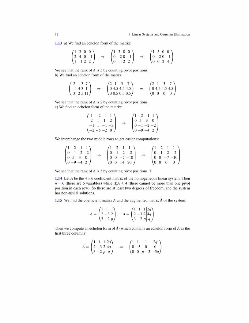
1.13 a) We find an echelon form of the matrix:1 3 0 02 4 0 −11 −1 2 2
⇒
1 3 0 00 −2 0 −10 −4 2 2
⇒
1 3 0 00 −2 0 −10 0 2 4
We see that the rank of A is 3 by counting pivot positions.b) We find an echelon form of the matrix: 2 1 3 7
−1 4 3 13 2 5 11
⇒
2 1 3 70 4.5 4.5 4.50 0.5 0.5 0.5
⇒
2 1 3 70 4.5 4.5 4.50 0 0 0
We see that the rank of A is 2 by counting pivot positions.c) We find an echelon form of the matrix:
1 −2 −1 12 1 1 2−1 1 −1 −3−2 −5 −2 0
⇒
1 −2 −1 10 5 3 00 −1 −2 −20 −9 −4 2
We interchange the two middle rows to get easier computations:
1 −2 −1 10 −1 −2 −20 5 3 00 −9 −4 2
⇒
1 −2 −1 10 −1 −2 −20 0 −7 −100 0 14 20
⇒
1 −2 −1 10 −1 −2 −20 0 −7 −100 0 0 0
We see that the rank of A is 3 by counting pivot positions. T
1.14 Let A be the 4×6 coefficient matrix of the homogeneous linear system. Thenn = 6 (there are 6 variables) while rkA ≤ 4 (there cannot be more than one pivotposition in each row). So there are at least two degrees of freedom, and the systemhas non-trivial solutions.
1.15 We find the coefficient matrix A and the augmented matrix A of the system:
A =
1 1 12 −3 23 −2 p
, A =
1 1 1 2q2 −3 2 4q3 −2 p q
Then we compute an echelon form of A (which contains an echelon form of A as thefirst three columns):
A =
1 1 1 2q2 −3 2 4q3 −2 p q
⇒
1 1 1 2q0 −5 0 00 0 p−3 −5q

1.3 Solutions 13
By counting pivot positions, we see that the ranks are given by
rkA =
{3 p 6= 32 p = 3
rk A =
{3 p 6= 3 or q 6= 02 p = 3 and q = 0
The linear system has one solution if p 6= 3, no solutions if p = 3 and q 6= 0, andinfinitely many solutions (one degree of freedom) if p = 3 and q = 0.
1.16 Midterm Exam in GRA6035 on 24/09/2010, Problem 3We compute an echelon form of A using elementary row operations, and get
A =
2 5 −3 −4 84 7 −4 −3 96 9 −5 −2 4
99K
2 5 −3 −4 80 −3 2 5 −70 0 0 0 −6
Hence A has rank 3.
1.17 Mock Midterm Exam in GRA6035 on 09/2010, Problem 3We compute an echelon form of A using elementary row operations, and get
A =
1 2 −5 0 −12 5 −8 4 3−3 −9 9 −7 −23 10 −7 11 7
99K
1 2 −5 0 −10 1 2 4 50 0 0 5 100 0 0 0 0
Hence A has rank 3.
1.18 Midterm Exam in GRA6035 on 24/05/2011, Problem 3We compute an echelon form of A using elementary row operations, and get
A =
2 10 6 81 5 4 113 15 7 −2
99K
1 5 4 110 0 1 70 0 0 0
Hence A has rank 2.

Previous: Lecture 1 Contents Next: Lecture 3
Lecture 2Matrices and Matrix Algebra
2.1 Main concepts
An m× n matrix is a rectangular array of numbers (with m rows and n columns).The entry of the matrix A in row i and column j is denoted ai j. The usual notation is
A = (ai j) =
a11 a12 . . . a1na21 a22 . . . a2n
......
. . ....
am1 am2 . . . amn
The matrix A is called square if m = n. A main diagonal of a square matrix consistsof the entries a11,a22, . . . ,ann, and the matrix is called a diagonal matrix if all otherentries are zero. It is called upper triangular if all entries below the main diagonalare zero.
We may add, subtract and mulitiply matrices of compatible dimensions, and writeA+B, A−B and A ·B. We may also multiply a number with a matrix and transposea matrix, and we write c ·A for scalar multiplication and AT for the transpose of A.A square matrix is called symmetric if AT = A.
The zero matrix 0 is the matrix where all entries are zero, and the identity matrixI is the diagonal matrix
I =
1 0 . . . 00 1 . . . 0...
.... . .
...0 0 . . . 1
The identity matrix has the property that I ·A = A · I = A for any matrix A. Matrixmultiplication is in general not commutative, so A ·B 6= B ·A. Otherwise, computa-tions with matrices follow similar rules as multiplication with numbers.
Problems Lecture 2 Solutions
16 2 Matrices and Matrix Algebra
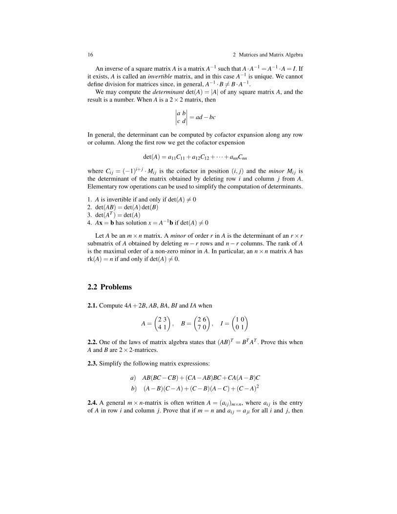
An inverse of a square matrix A is a matrix A−1 such that A ·A−1 = A−1 ·A = I. Ifit exists, A is called an invertible matrix, and in this case A−1 is unique. We cannotdefine division for matrices since, in general, A−1 ·B 6= B ·A−1.
We may compute the determinant det(A) = |A| of any square matrix A, and theresult is a number. When A is a 2×2 matrix, then∣∣∣∣a b
c d
∣∣∣∣= ad−bc
In general, the determinant can be computed by cofactor expansion along any rowor column. Along the first row we get the cofactor expension
det(A) = a11C11 +a12C12 + · · ·+annCnn
where Ci j = (−1)i+ j ·Mi j is the cofactor in position (i, j) and the minor Mi j isthe determinant of the matrix obtained by deleting row i and column j from A.Elementary row operations can be used to simplify the computation of determinants.
1. A is invertible if and only if det(A) 6= 02. det(AB) = det(A)det(B)3. det(AT ) = det(A)4. Ax = b has solution x = A−1b if det(A) 6= 0
Let A be an m×n matrix. A minor of order r in A is the determinant of an r× rsubmatrix of A obtained by deleting m− r rows and n− r columns. The rank of Ais the maximal order of a non-zero minor in A. In particular, an n×n matrix A hasrk(A) = n if and only if det(A) 6= 0.
2.2 Problems
2.1. Compute 4A+2B, AB, BA, BI and IA when
A =
(2 34 1
), B =
(2 67 0
), I =
(1 00 1
)2.2. One of the laws of matrix algebra states that (AB)T = BT AT . Prove this whenA and B are 2×2-matrices.
2.3. Simplify the following matrix expressions:
a) AB(BC−CB)+(CA−AB)BC+CA(A−B)C
b) (A−B)(C−A)+(C−B)(A−C)+(C−A)2
2.4. A general m× n-matrix is often written A = (ai j)m×n, where ai j is the entryof A in row i and column j. Prove that if m = n and ai j = a ji for all i and j, then
2.2 Problems 17
A = AT . Give a concrete example of a matrix with this property, and explain why itis reasonable to call a matrix A symmetric when A = AT .
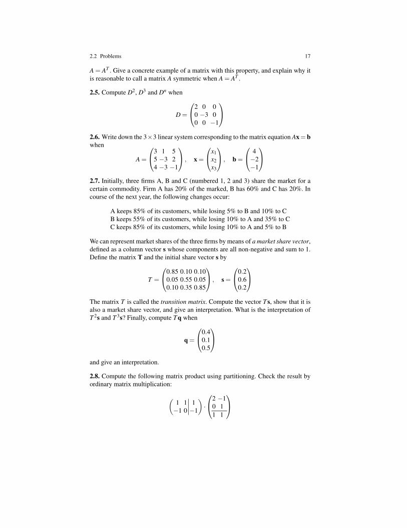
2.5. Compute D2, D3 and Dn when
D =
2 0 00 −3 00 0 −1
2.6. Write down the 3×3 linear system corresponding to the matrix equation Ax= bwhen
A =
3 1 55 −3 24 −3 −1
, x =
x1x2x3
, b =
4−2−1
2.7. Initially, three firms A, B and C (numbered 1, 2 and 3) share the market for acertain commodity. Firm A has 20% of the marked, B has 60% and C has 20%. Incourse of the next year, the following changes occur:
A keeps 85% of its customers, while losing 5% to B and 10% to CB keeps 55% of its customers, while losing 10% to A and 35% to CC keeps 85% of its customers, while losing 10% to A and 5% to B
We can represent market shares of the three firms by means of a market share vector,defined as a column vector s whose components are all non-negative and sum to 1.Define the matrix T and the initial share vector s by
T =
0.85 0.10 0.100.05 0.55 0.050.10 0.35 0.85
, s =
0.20.60.2
The matrix T is called the transition matrix. Compute the vector T s, show that it isalso a market share vector, and give an interpretation. What is the interpretation ofT 2s and T 3s? Finally, compute T q when
q =
0.40.10.5
and give an interpretation.
2.8. Compute the following matrix product using partitioning. Check the result byordinary matrix multiplication:
(1 1 1−1 0 −1
)·
2 −10 11 1
18 2 Matrices and Matrix Algebra
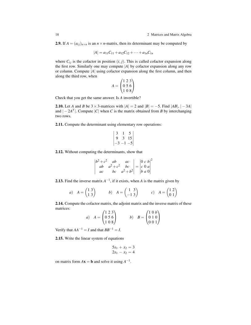
2.9. If A = (ai j)n×n is an n×n-matrix, then its determinant may be computed by
|A|= a11C11 +a12C12 + · · ·+a1nC1n
where Ci j is the cofactor in position (i, j). This is called cofactor expansion alongthe first row. Similarly one may compute |A| by cofactor expansion along any rowor column. Compute |A| using cofactor expansion along the first column, and thenalong the third row, when
A =
1 2 30 5 61 0 8
Check that you get the same answer. Is A invertible?
2.10. Let A and B be 3× 3-matrices with |A| = 2 and |B| = −5. Find |AB|, |− 3A|and |−2AT |. Compute |C| when C is the matrix obtained from B by interchangingtwo rows.
2.11. Compute the determinant using elementary row operations:∣∣∣∣∣∣3 1 59 3 15−3 −1 −5
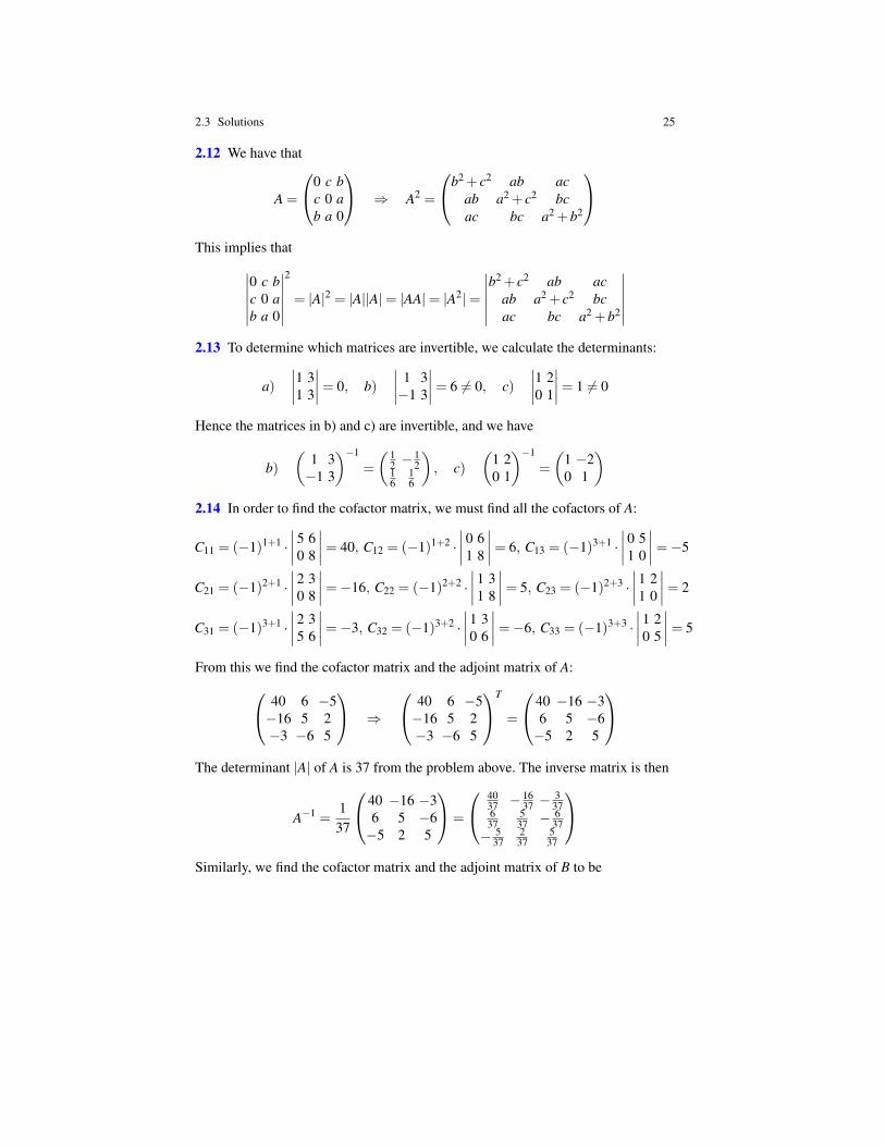
∣∣∣∣∣∣2.12. Without computing the determinants, show that∣∣∣∣∣∣
b2 + c2 ab acab a2 + c2 bcac bc a2 +b2
∣∣∣∣∣∣=∣∣∣∣∣∣0 c bc 0 ab a 0
∣∣∣∣∣∣2
2.13. Find the inverse matrix A−1, if it exists, when A is the matrix given by
a) A =
(1 31 3
)b) A =
(1 3−1 3
)c) A =
(1 20 1
)2.14. Compute the cofactor matrix, the adjoint matrix and the inverse matrix of thesematrices:
a) A =
1 2 30 5 61 0 8
b) B =
1 0 b0 1 00 0 1
Verify that AA−1 = I and that BB−1 = I.
2.15. Write the linear system of equations
5x1 + x2 = 32x1 − x2 = 4
on matrix form Ax = b and solve it using A−1.
2.2 Problems 19
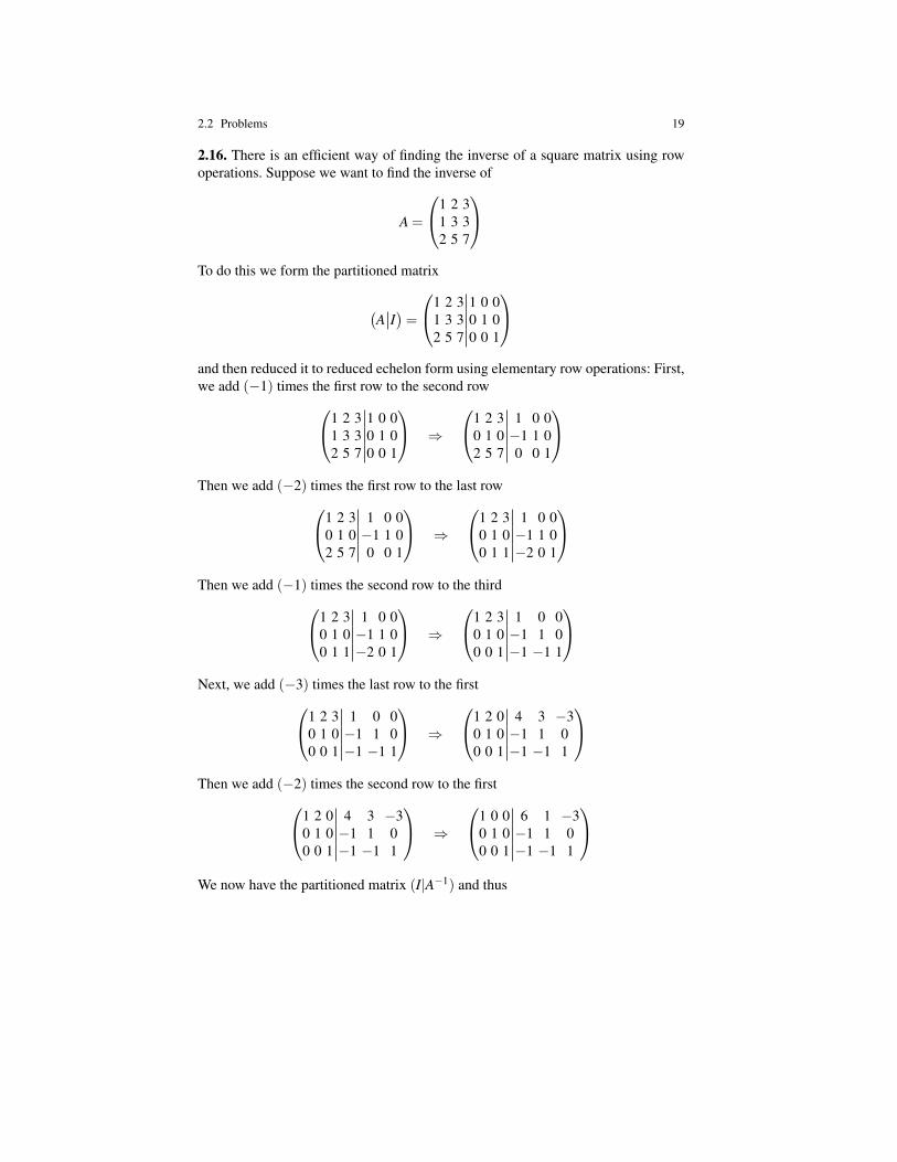
2.16. There is an efficient way of finding the inverse of a square matrix using rowoperations. Suppose we want to find the inverse of
A =
1 2 31 3 32 5 7
To do this we form the partitioned matrix
(A I)=
1 2 3 1 0 01 3 3 0 1 02 5 7 0 0 1
and then reduced it to reduced echelon form using elementary row operations: First,we add (−1) times the first row to the second row1 2 3 1 0 0
1 3 3 0 1 02 5 7 0 0 1
⇒
1 2 3 1 0 00 1 0 −1 1 02 5 7 0 0 1
Then we add (−2) times the first row to the last row1 2 3 1 0 0
0 1 0 −1 1 02 5 7 0 0 1
⇒
1 2 3 1 0 00 1 0 −1 1 00 1 1 −2 0 1
Then we add (−1) times the second row to the third1 2 3 1 0 0
0 1 0 −1 1 00 1 1 −2 0 1
⇒
1 2 3 1 0 00 1 0 −1 1 00 0 1 −1 −1 1
Next, we add (−3) times the last row to the first1 2 3 1 0 0
0 1 0 −1 1 00 0 1 −1 −1 1
⇒
1 2 0 4 3 −30 1 0 −1 1 00 0 1 −1 −1 1
Then we add (−2) times the second row to the first1 2 0 4 3 −3
0 1 0 −1 1 00 0 1 −1 −1 1
⇒
1 0 0 6 1 −30 1 0 −1 1 00 0 1 −1 −1 1
We now have the partitioned matrix (I|A−1) and thus
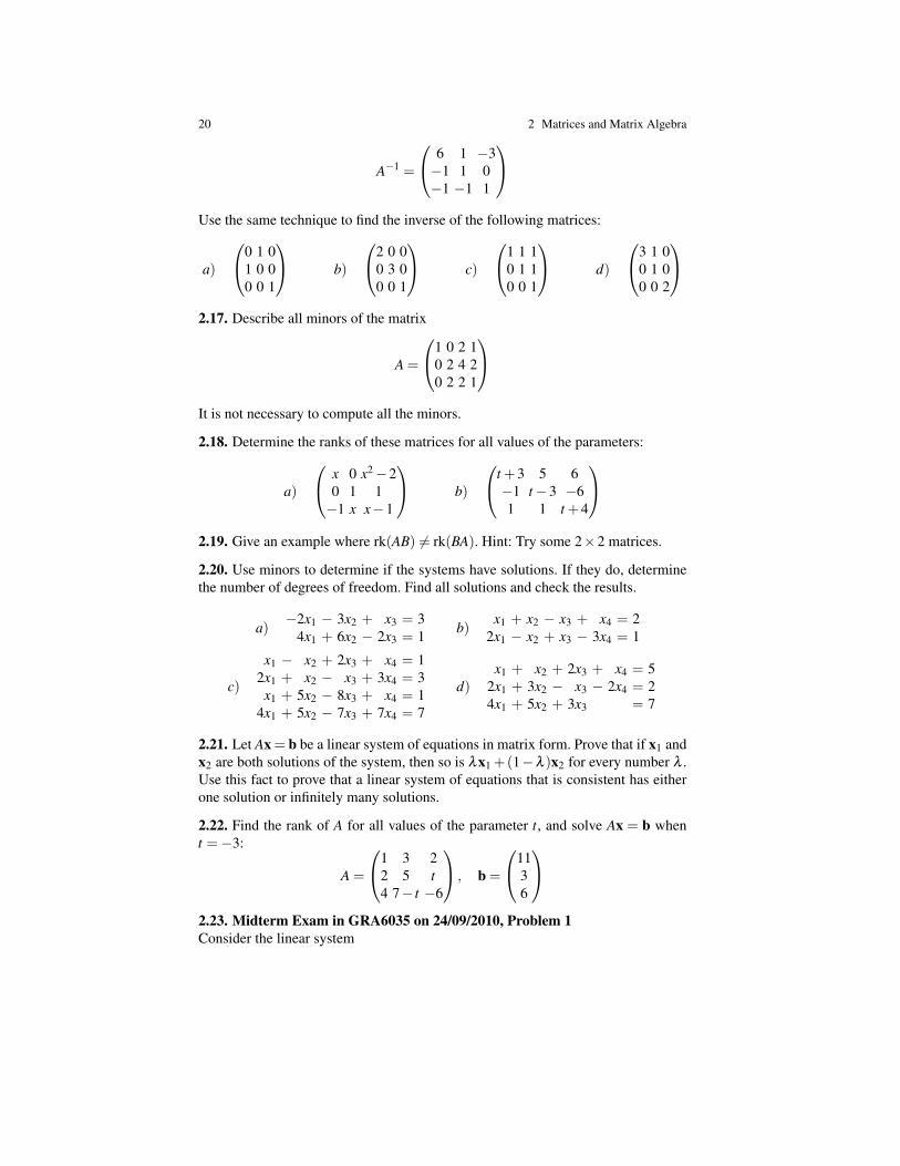
20 2 Matrices and Matrix Algebra
A−1 =
6 1 −3−1 1 0−1 −1 1
Use the same technique to find the inverse of the following matrices:
a)
0 1 01 0 00 0 1
b)
2 0 00 3 00 0 1
c)
1 1 10 1 10 0 1
d)
3 1 00 1 00 0 2
2.17. Describe all minors of the matrix
A =
1 0 2 10 2 4 20 2 2 1
It is not necessary to compute all the minors.
2.18. Determine the ranks of these matrices for all values of the parameters:
a)
x 0 x2−20 1 1−1 x x−1
b)
t +3 5 6−1 t−3 −61 1 t +4
2.19. Give an example where rk(AB) 6= rk(BA). Hint: Try some 2×2 matrices.
2.20. Use minors to determine if the systems have solutions. If they do, determinethe number of degrees of freedom. Find all solutions and check the results.
a)−2x1 − 3x2 + x3 = 3
4x1 + 6x2 − 2x3 = 1 b)x1 + x2 − x3 + x4 = 2
2x1 − x2 + x3 − 3x4 = 1
c)
x1 − x2 + 2x3 + x4 = 12x1 + x2 − x3 + 3x4 = 3
x1 + 5x2 − 8x3 + x4 = 14x1 + 5x2 − 7x3 + 7x4 = 7
d)x1 + x2 + 2x3 + x4 = 5
2x1 + 3x2 − x3 − 2x4 = 24x1 + 5x2 + 3x3 = 7
2.21. Let Ax = b be a linear system of equations in matrix form. Prove that if x1 andx2 are both solutions of the system, then so is λx1 +(1−λ )x2 for every number λ .Use this fact to prove that a linear system of equations that is consistent has eitherone solution or infinitely many solutions.
2.22. Find the rank of A for all values of the parameter t, and solve Ax = b whent =−3:
A =
1 3 22 5 t4 7− t −6
, b =
1136
2.23. Midterm Exam in GRA6035 on 24/09/2010, Problem 1Consider the linear system
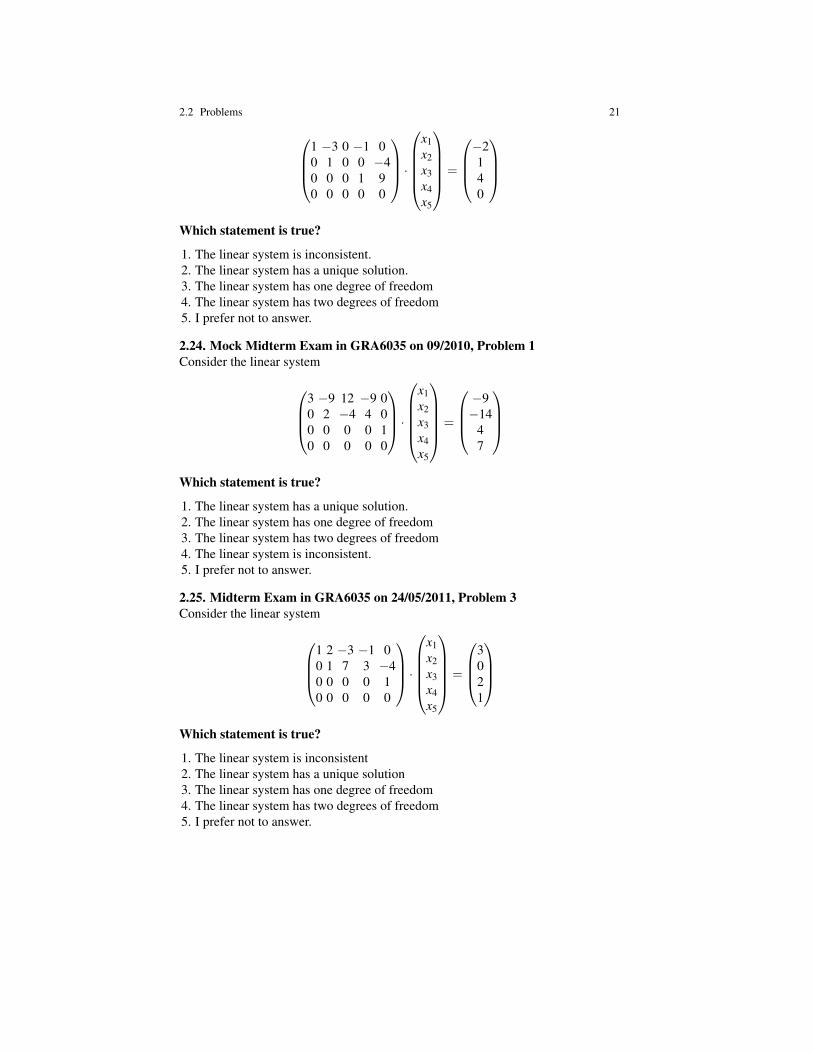
2.2 Problems 211 −3 0 −1 00 1 0 0 −40 0 0 1 90 0 0 0 0
·
x1x2x3x4x5
=
−2140
Which statement is true?
1. The linear system is inconsistent.2. The linear system has a unique solution.3. The linear system has one degree of freedom4. The linear system has two degrees of freedom5. I prefer not to answer.
2.24. Mock Midterm Exam in GRA6035 on 09/2010, Problem 1Consider the linear system
3 −9 12 −9 00 2 −4 4 00 0 0 0 10 0 0 0 0
·
x1x2x3x4x5
=
−9−14
47
Which statement is true?
1. The linear system has a unique solution.2. The linear system has one degree of freedom3. The linear system has two degrees of freedom4. The linear system is inconsistent.5. I prefer not to answer.
2.25. Midterm Exam in GRA6035 on 24/05/2011, Problem 3Consider the linear system
1 2 −3 −1 00 1 7 3 −40 0 0 0 10 0 0 0 0
·
x1x2x3x4x5
=
3021
Which statement is true?
1. The linear system is inconsistent2. The linear system has a unique solution3. The linear system has one degree of freedom4. The linear system has two degrees of freedom5. I prefer not to answer.
22 2 Matrices and Matrix Algebra
2.3 Solutions
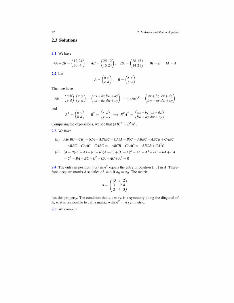
2.1 We have
4A+2B =
(12 2430 4
), AB =
(25 1215 24
), BA =
(28 1214 21
), BI = B, IA = A
2.2 Let
A =
(a bc d
), B =
(x yz w
)Then we have
AB =
(a bc d
)(x yz w
)=
(ax+bz bw+aycx+dz dw+ cy
)=⇒ (AB)T =
(ax+bz cx+dzbw+ay dw+ cy
)and
AT =
(a cb d
), BT =
(x zy w
)=⇒ BT AT =
(ax+bz cx+dzbw+ay dw+ cy
)Comparing the expressions, we see that (AB)T = BT AT .
2.3 We have
(a) AB(BC−CB)+(CA−AB)BC+CA(A−B)C = ABBC−ABCB+CABC
−ABBC+CAAC−CABC =−ABCB+CAAC =−ABCB+CA2C
(b) (A−B)(C−A)+(C−B)(A−C)+(C−A)2 = AC−A2−BC+BA+CA
−C2−BA+BC+C2−CA−AC+A2 = 0
2.4 The entry in position ( j, i) in AT equals the entry in position (i, j) in A. There-fore, a square matrix A satisfies AT = A if ai j = a ji. The matrix
A =
13 3 23 −2 42 4 3
has this property. The condition that ai j = a ji is a symmetry along the diagonal ofA, so it is reasonable to call a matrix with AT = A symmetric.
2.5 We compute
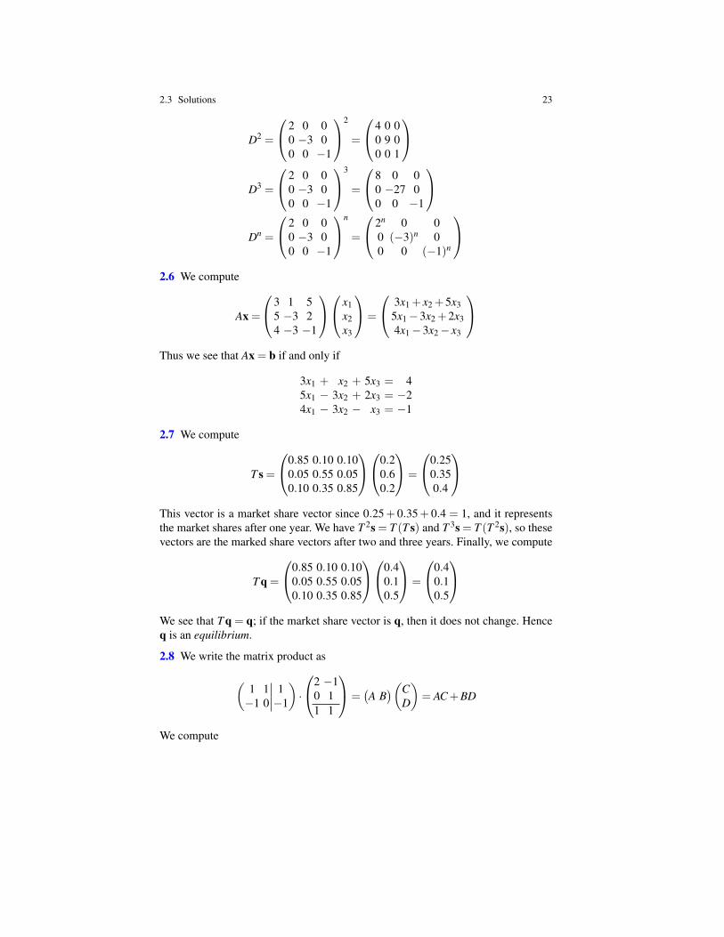
2.3 Solutions 23
D2 =
2 0 00 −3 00 0 −1
2
=
4 0 00 9 00 0 1
D3 =
2 0 00 −3 00 0 −1
3
=
8 0 00 −27 00 0 −1
Dn =
2 0 00 −3 00 0 −1
n
=
2n 0 00 (−3)n 00 0 (−1)n
2.6 We compute
Ax =
3 1 55 −3 24 −3 −1
x1x2x3
=
3x1 + x2 +5x35x1−3x2 +2x34x1−3x2− x3
Thus we see that Ax = b if and only if
3x1 + x2 + 5x3 = 45x1 − 3x2 + 2x3 = −24x1 − 3x2 − x3 = −1
2.7 We compute
T s =
0.85 0.10 0.100.05 0.55 0.050.10 0.35 0.85
0.20.60.2
=
0.250.350.4
This vector is a market share vector since 0.25+ 0.35+ 0.4 = 1, and it representsthe market shares after one year. We have T 2s = T (T s) and T 3s = T (T 2s), so thesevectors are the marked share vectors after two and three years. Finally, we compute
T q =
0.85 0.10 0.100.05 0.55 0.050.10 0.35 0.85
0.40.10.5
=
0.40.10.5
We see that T q = q; if the market share vector is q, then it does not change. Henceq is an equilibrium.
2.8 We write the matrix product as
(1 1 1−1 0 −1
)·
2 −10 11 1
=(A B)(C
D
)= AC+BD
We compute
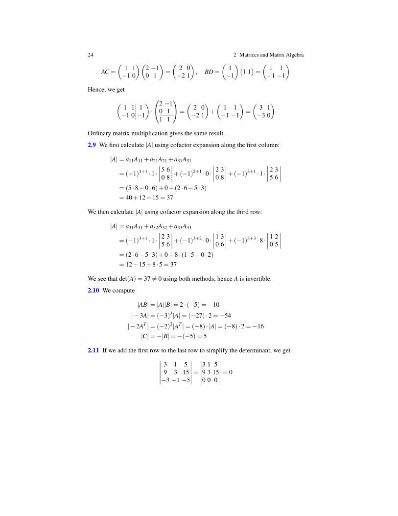
24 2 Matrices and Matrix Algebra
AC =
(1 1−1 0
)(2 −10 1
)=
(2 0−2 1
), BD =
(1−1
)(1 1)=
(1 1−1 −1
)Hence, we get
(1 1 1−1 0 −1
)·
2 −10 11 1
=
(2 0−2 1
)+
(1 1−1 −1
)=
(3 1−3 0
)
Ordinary matrix multiplication gives the same result.
2.9 We first calculate |A| using cofactor expansion along the first column:
|A|= a11A11 +a21A21 +a31A31
= (−1)1+1 ·1 ·∣∣∣∣5 60 8
∣∣∣∣+(−1)2+1 ·0 ·∣∣∣∣2 30 8
∣∣∣∣+(−1)3+1 ·1 ·∣∣∣∣2 35 6
∣∣∣∣= (5 ·8−0 ·6)+0+(2 ·6−5 ·3)= 40+12−15 = 37
We then calculate |A| using cofactor expansion along the third row:
|A|= a31A31 +a32A32 +a33A33
= (−1)3+1 ·1 ·∣∣∣∣2 35 6
∣∣∣∣+(−1)3+2 ·0 ·∣∣∣∣1 30 6
∣∣∣∣+(−1)3+3 ·8 ·∣∣∣∣1 20 5
∣∣∣∣= (2 ·6−5 ·3)+0+8 · (1 ·5−0 ·2)= 12−15+8 ·5 = 37
We see that det(A) = 37 6= 0 using both methods, hence A is invertible.
2.10 We compute
|AB|= |A||B|= 2 · (−5) =−10
|−3A|= (−3)3|A|= (−27) ·2 =−54
|−2AT |= (−2)3|AT |= (−8) · |A|= (−8) ·2 =−16|C|=−|B|=−(−5) = 5
2.11 If we add the first row to the last row to simplify the determinant, we get∣∣∣∣∣∣3 1 59 3 15−3 −1 −5
∣∣∣∣∣∣=∣∣∣∣∣∣3 1 59 3 150 0 0
∣∣∣∣∣∣= 0
2.3 Solutions 25
2.12 We have that
A =
0 c bc 0 ab a 0
⇒ A2 =
b2 + c2 ab acab a2 + c2 bcac bc a2 +b2
This implies that∣∣∣∣∣∣
0 c bc 0 ab a 0
∣∣∣∣∣∣2
= |A|2 = |A||A|= |AA|= |A2|=
∣∣∣∣∣∣b2 + c2 ab ac
ab a2 + c2 bcac bc a2 +b2
∣∣∣∣∣∣2.13 To determine which matrices are invertible, we calculate the determinants:
a)∣∣∣∣1 31 3
∣∣∣∣= 0, b)∣∣∣∣ 1 3−1 3
∣∣∣∣= 6 6= 0, c)∣∣∣∣1 20 1
∣∣∣∣= 1 6= 0
Hence the matrices in b) and c) are invertible, and we have
b)(
1 3−1 3
)−1
=
( 12 −
12
16
16
), c)
(1 20 1
)−1
=
(1 −20 1
)2.14 In order to find the cofactor matrix, we must find all the cofactors of A:
C11 = (−1)1+1 ·∣∣∣∣5 60 8
∣∣∣∣= 40, C12 = (−1)1+2 ·∣∣∣∣0 61 8
∣∣∣∣= 6, C13 = (−1)3+1 ·∣∣∣∣0 51 0
∣∣∣∣=−5
C21 = (−1)2+1 ·∣∣∣∣2 30 8
∣∣∣∣=−16, C22 = (−1)2+2 ·∣∣∣∣1 31 8
∣∣∣∣= 5, C23 = (−1)2+3 ·∣∣∣∣1 21 0
∣∣∣∣= 2
C31 = (−1)3+1 ·∣∣∣∣2 35 6
∣∣∣∣=−3, C32 = (−1)3+2 ·∣∣∣∣1 30 6
∣∣∣∣=−6, C33 = (−1)3+3 ·∣∣∣∣1 20 5
∣∣∣∣= 5
From this we find the cofactor matrix and the adjoint matrix of A: 40 6 −5−16 5 2−3 −6 5
⇒
40 6 −5−16 5 2−3 −6 5
T
=
40 −16 −36 5 −6−5 2 5
The determinant |A| of A is 37 from the problem above. The inverse matrix is then
A−1 =1
37
40 −16 −36 5 −6−5 2 5
=
4037 −
1637 −
337
637
537 −
637
− 537
237
537
Similarly, we find the cofactor matrix and the adjoint matrix of B to be
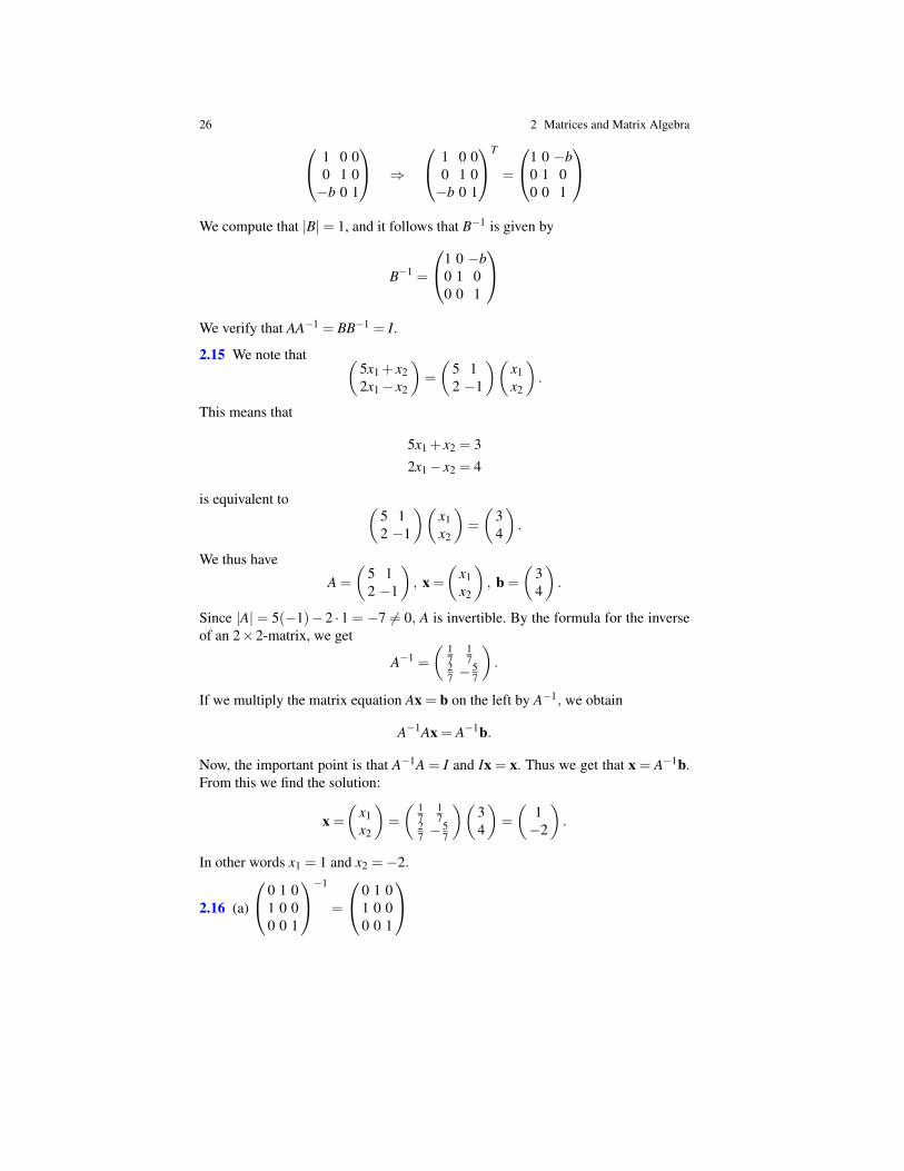
26 2 Matrices and Matrix Algebra 1 0 00 1 0−b 0 1
⇒
1 0 00 1 0−b 0 1
T
=
1 0 −b0 1 00 0 1
We compute that |B|= 1, and it follows that B−1 is given by
B−1 =
1 0 −b0 1 00 0 1
We verify that AA−1 = BB−1 = I.
2.15 We note that (5x1 + x22x1− x2
)=
(5 12 −1
)(x1x2
).
This means that
5x1 + x2 = 32x1− x2 = 4
is equivalent to (5 12 −1
)(x1x2
)=
(34
).
We thus have
A =
(5 12 −1
), x =
(x1x2
), b =
(34
).
Since |A| = 5(−1)−2 ·1 = −7 6= 0, A is invertible. By the formula for the inverseof an 2×2-matrix, we get
A−1 =
( 17
17
27 −
57
).
If we multiply the matrix equation Ax = b on the left by A−1, we obtain
A−1Ax = A−1b.
Now, the important point is that A−1A = I and Ix = x. Thus we get that x = A−1b.From this we find the solution:
x =
(x1x2
)=
( 17
17
27 −
57
)(34
)=
(1−2
).
In other words x1 = 1 and x2 =−2.
2.16 (a)
0 1 01 0 00 0 1
−1
=
0 1 01 0 00 0 1
2.3 Solutions 27
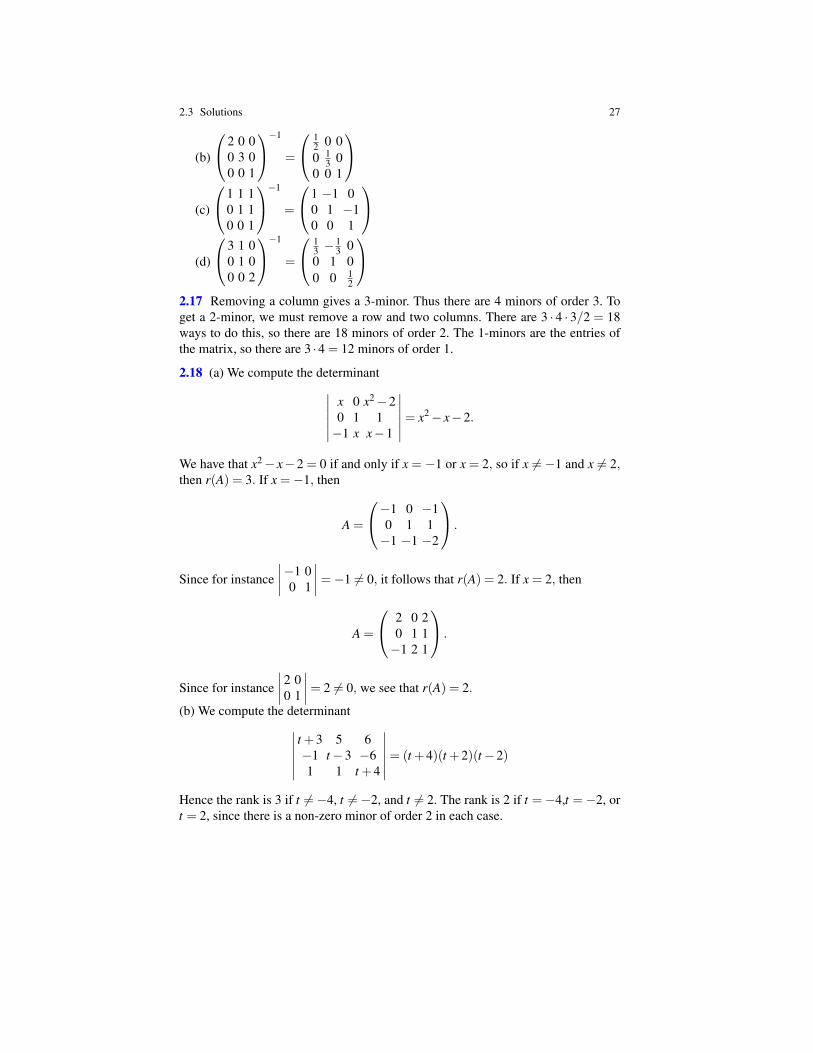
(b)
2 0 00 3 00 0 1
−1
=
12 0 00 1
3 00 0 1
(c)
1 1 10 1 10 0 1
−1
=
1 −1 00 1 −10 0 1
(d)
3 1 00 1 00 0 2
−1
=
13 −
13 0
0 1 00 0 1
2
2.17 Removing a column gives a 3-minor. Thus there are 4 minors of order 3. Toget a 2-minor, we must remove a row and two columns. There are 3 · 4 · 3/2 = 18ways to do this, so there are 18 minors of order 2. The 1-minors are the entries ofthe matrix, so there are 3 ·4 = 12 minors of order 1.
2.18 (a) We compute the determinant∣∣∣∣∣∣x 0 x2−20 1 1−1 x x−1
∣∣∣∣∣∣= x2− x−2.
We have that x2− x−2 = 0 if and only if x = −1 or x = 2, so if x 6=−1 and x 6= 2,then r(A) = 3. If x =−1, then
A =
−1 0 −10 1 1−1 −1 −2
.
Since for instance∣∣∣∣−1 0
0 1
∣∣∣∣=−1 6= 0, it follows that r(A) = 2. If x = 2, then
A =
2 0 20 1 1−1 2 1
.
Since for instance∣∣∣∣2 00 1
∣∣∣∣= 2 6= 0, we see that r(A) = 2.
(b) We compute the determinant∣∣∣∣∣∣t +3 5 6−1 t−3 −61 1 t +4
∣∣∣∣∣∣= (t +4)(t +2)(t−2)
Hence the rank is 3 if t 6=−4, t 6=−2, and t 6= 2. The rank is 2 if t =−4,t =−2, ort = 2, since there is a non-zero minor of order 2 in each case.
28 2 Matrices and Matrix Algebra
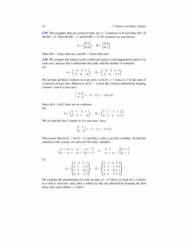
2.19 The examples that are easiest to find, are 2×2-matrices A,B such that AB 6= 0but BA = 0. Then rk(AB)≥ 1 and rk(BA) = 0. For instance we can choose
A =
(0 10 0
), B =
(0 00 1
)Then AB = A has rank one, and BA = 0 has rank zero.
2.20 We compute the minors in the coefficient matrix A and augmented matrix A ineach case, and use this to determine the ranks and the number of solutions.(a)
A =
(−2 −3 14 6 −2
), A =
(−2 −3 1 34 6 −2 1
)We see that all three 2-minors in A are zero, so rk(A) = 1 (since A 6= 0, the rank ofA must be at least one). Moreover, rk(A) = 2 since the 2-minor obtained by keepingcolumn 1 and 4 is non-zero:∣∣∣∣−2 3
4 1
∣∣∣∣=−2−12 =−14 6= 0
Since rkA < rk A, there are no solutions.(b)
A =
(1 1 −1 12 −1 1 −3
), A =
(1 1 −1 1 22 −1 1 −3 1
)We see that the first 2-minor in A is non-zero, since∣∣∣∣1 1
2 −1
∣∣∣∣=−1−2 =−3 6= 0
This means that rk(A) = rk(A) = 2, and that x3 and x4 are free variables. To find thesolution of the system, we solve for the basic variables:
x1 + x2 = x3 − x4 + 22x1 − x2 = −x3 + 3x4 + 1 ⇒ x1 = 2
3 x4 + 1x2 = x3 − 5
3 x4 + 1
(c)
A =
1 −1 2 12 1 −1 31 5 −8 14 5 −7 7
, A =
1 −1 2 1 12 1 −1 3 31 5 −8 1 14 5 −7 7 7
We compute the determinant of A and see that |A|= 0. Next, we look for a 3-minorin A that is non-zero, and (after a while) try the one obtained by keeping the firstthree rows and column 1, 2 and 4:
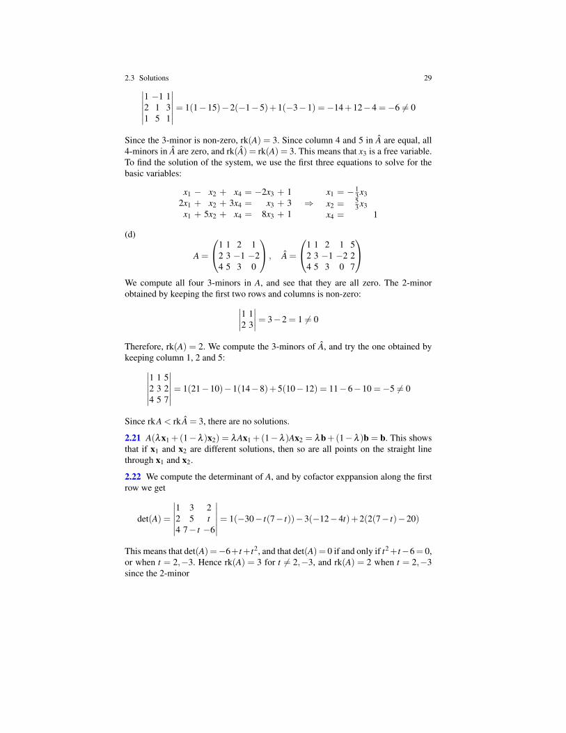
2.3 Solutions 29∣∣∣∣∣∣1 −1 12 1 31 5 1
∣∣∣∣∣∣= 1(1−15)−2(−1−5)+1(−3−1) =−14+12−4 =−6 6= 0
Since the 3-minor is non-zero, rk(A) = 3. Since column 4 and 5 in A are equal, all4-minors in A are zero, and rk(A) = rk(A) = 3. This means that x3 is a free variable.To find the solution of the system, we use the first three equations to solve for thebasic variables:
x1 − x2 + x4 = −2x3 + 12x1 + x2 + 3x4 = x3 + 3
x1 + 5x2 + x4 = 8x3 + 1⇒
x1 = − 13 x3
x2 = 53 x3
x4 = 1
(d)
A =
1 1 2 12 3 −1 −24 5 3 0
, A =
1 1 2 1 52 3 −1 −2 24 5 3 0 7
We compute all four 3-minors in A, and see that they are all zero. The 2-minorobtained by keeping the first two rows and columns is non-zero:∣∣∣∣1 1
2 3
∣∣∣∣= 3−2 = 1 6= 0
Therefore, rk(A) = 2. We compute the 3-minors of A, and try the one obtained bykeeping column 1, 2 and 5:∣∣∣∣∣∣
1 1 52 3 24 5 7
∣∣∣∣∣∣= 1(21−10)−1(14−8)+5(10−12) = 11−6−10 =−5 6= 0
Since rkA < rk A = 3, there are no solutions.
2.21 A(λx1 +(1−λ )x2) = λAx1 +(1−λ )Ax2 = λb+(1−λ )b = b. This showsthat if x1 and x2 are different solutions, then so are all points on the straight linethrough x1 and x2.
2.22 We compute the determinant of A, and by cofactor exppansion along the firstrow we get
det(A) =
∣∣∣∣∣∣1 3 22 5 t4 7− t −6
∣∣∣∣∣∣= 1(−30− t(7− t))−3(−12−4t)+2(2(7− t)−20)
This means that det(A) =−6+t+t2, and that det(A) = 0 if and only if t2+t−6= 0,or when t = 2,−3. Hence rk(A) = 3 for t 6= 2,−3, and rk(A) = 2 when t = 2,−3since the 2-minor
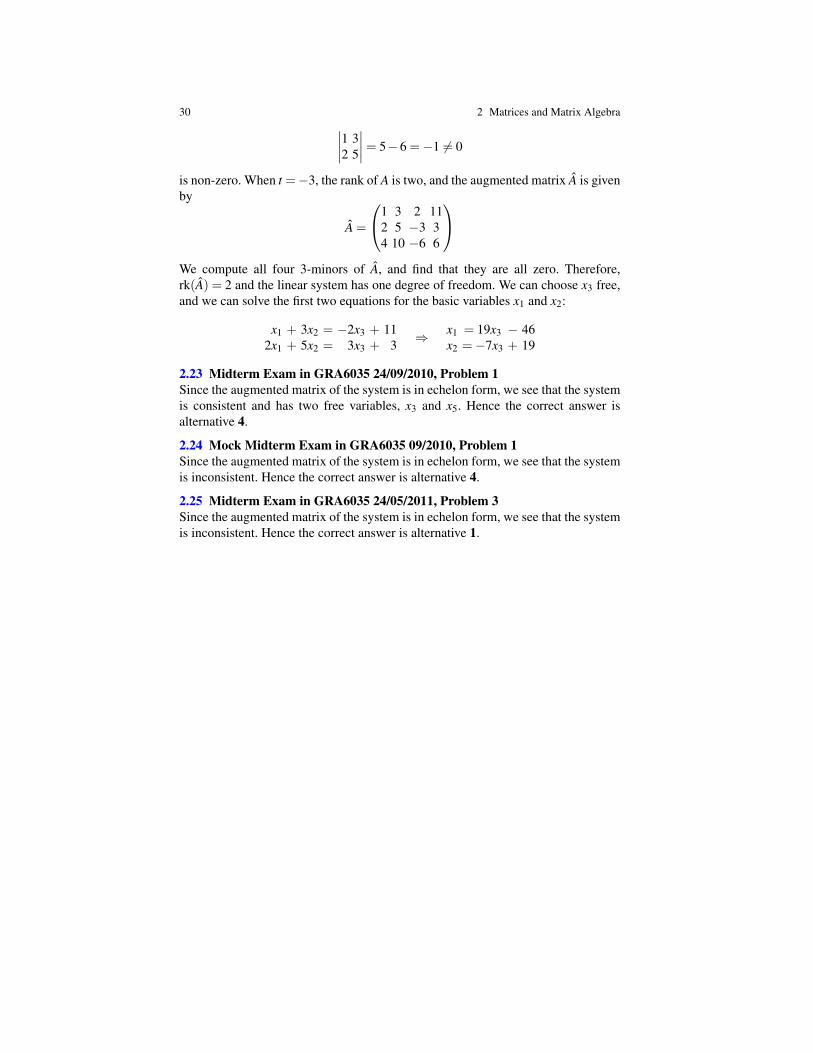
30 2 Matrices and Matrix Algebra∣∣∣∣1 32 5
∣∣∣∣= 5−6 =−1 6= 0
is non-zero. When t =−3, the rank of A is two, and the augmented matrix A is givenby
A =
1 3 2 112 5 −3 34 10 −6 6
We compute all four 3-minors of A, and find that they are all zero. Therefore,rk(A) = 2 and the linear system has one degree of freedom. We can choose x3 free,and we can solve the first two equations for the basic variables x1 and x2:
x1 + 3x2 = −2x3 + 112x1 + 5x2 = 3x3 + 3 ⇒ x1 = 19x3 − 46
x2 =−7x3 + 19
2.23 Midterm Exam in GRA6035 24/09/2010, Problem 1Since the augmented matrix of the system is in echelon form, we see that the systemis consistent and has two free variables, x3 and x5. Hence the correct answer isalternative 4.
2.24 Mock Midterm Exam in GRA6035 09/2010, Problem 1Since the augmented matrix of the system is in echelon form, we see that the systemis inconsistent. Hence the correct answer is alternative 4.
2.25 Midterm Exam in GRA6035 24/05/2011, Problem 3Since the augmented matrix of the system is in echelon form, we see that the systemis inconsistent. Hence the correct answer is alternative 1.
Previous: Lecture 2 Contents Next: Lecture 4
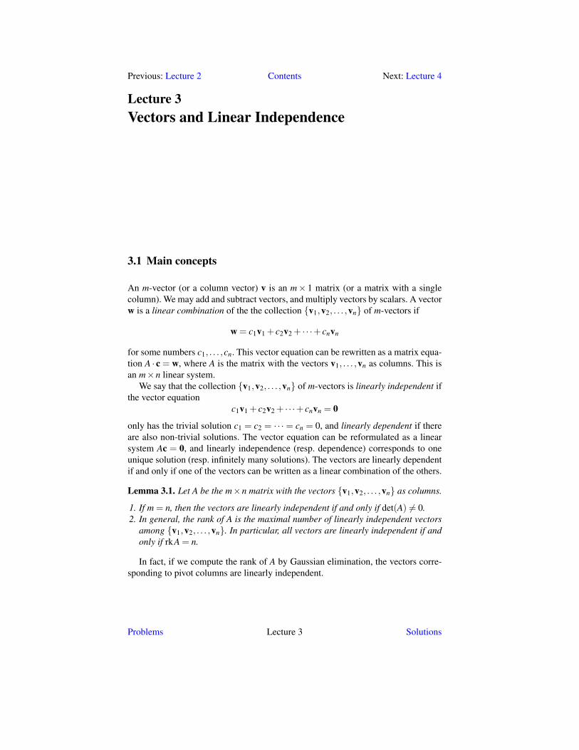
Lecture 3Vectors and Linear Independence
3.1 Main concepts
An m-vector (or a column vector) v is an m× 1 matrix (or a matrix with a singlecolumn). We may add and subtract vectors, and multiply vectors by scalars. A vectorw is a linear combination of the the collection {v1,v2, . . . ,vn} of m-vectors if
w = c1v1 + c2v2 + · · ·+ cnvn
for some numbers c1, . . . ,cn. This vector equation can be rewritten as a matrix equa-tion A · c = w, where A is the matrix with the vectors v1, . . . ,vn as columns. This isan m×n linear system.
We say that the collection {v1,v2, . . . ,vn} of m-vectors is linearly independent ifthe vector equation
c1v1 + c2v2 + · · ·+ cnvn = 0
only has the trivial solution c1 = c2 = · · ·= cn = 0, and linearly dependent if thereare also non-trivial solutions. The vector equation can be reformulated as a linearsystem Ac = 0, and linearly independence (resp. dependence) corresponds to oneunique solution (resp. infinitely many solutions). The vectors are linearly dependentif and only if one of the vectors can be written as a linear combination of the others.
Lemma 3.1. Let A be the m×n matrix with the vectors {v1,v2, . . . ,vn} as columns.
1. If m = n, then the vectors are linearly independent if and only if det(A) 6= 0.2. In general, the rank of A is the maximal number of linearly independent vectors
among {v1,v2, . . . ,vn}. In particular, all vectors are linearly independent if andonly if rkA = n.
In fact, if we compute the rank of A by Gaussian elimination, the vectors corre-sponding to pivot columns are linearly independent.
Problems Lecture 3 Solutions
32 3 Vectors and Linear Independence
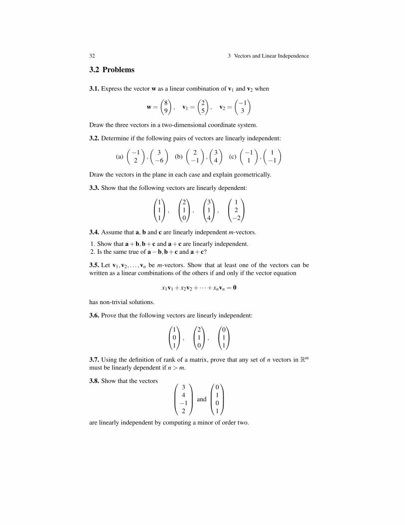
3.2 Problems
3.1. Express the vector w as a linear combination of v1 and v2 when
w =
(89
), v1 =
(25
), v2 =
(−13
)Draw the three vectors in a two-dimensional coordinate system.
3.2. Determine if the following pairs of vectors are linearly independent:
(a)(−12
),
(3−6
)(b)(
2−1
),
(34
)(c)(−11
),
(1−1
)Draw the vectors in the plane in each case and explain geometrically.
3.3. Show that the following vectors are linearly dependent:111
,
210
,
314
,
12−2
3.4. Assume that a, b and c are linearly independent m-vectors.
1. Show that a+b,b+ c and a+ c are linearly independent.2. Is the same true of a−b,b+ c and a+ c?
3.5. Let v1,v2, . . . ,vn be m-vectors. Show that at least one of the vectors can bewritten as a linear combinations of the others if and only if the vector equation
x1v1 + x2v2 + · · ·+ xnvn = 0
has non-trivial solutions.
3.6. Prove that the following vectors are linearly independent:101
,
210
,
011
3.7. Using the definition of rank of a matrix, prove that any set of n vectors in Rm
must be linearly dependent if n > m.
3.8. Show that the vectors 34−12
and
0101
are linearly independent by computing a minor of order two.
3.2 Problems 33
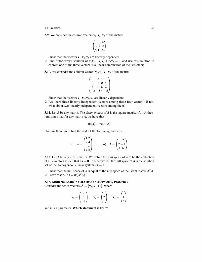
3.9. We consider the column vectors v1,v2,v3 of the matrix1 2 43 7 05 11 8
1. Show that the vectors v1,v2,v3 are linearly dependent.2. Find a non-trivial solution of x1v1 + x2v2 + x3v3 = 0, and use this solution to
express one of the three vectors as a linear combination of the two others.
3.10. We consider the column vectors v1,v2,v3,v4 of the matrix1 2 4 −13 7 0 45 11 8 2−2 −5 4 −5
1. Show that the vectors v1,v2,v3,v4 are linearly dependent.2. Are there three linearly independent vectors among these four vectors? If not,
what about two linearly independent vectors among them?
3.11. Let A be any matrix. The Gram matrix of A is the square matrix AT A. A theo-rem states that for any matrix A, we have that
rk(A) = rk(AT A)
Use this theorem to find the rank of the following matrices:
a) A =
1 22 43 64 8
b) A =
1 22 −13 6
3.12. Let A be any m×n-matrix. We define the null space of A to be the collectionof all n-vectors x such that Ax = 0. In other words, the null space of A is the solutionset of the homogeneous linear system Ax = 0.
1. Show that the null space of A is equal to the null space of the Gram matrix AT A.2. Prove that rk(A) = rk(AT A).
3.13. Midterm Exam in GRA6035 on 24/09/2010, Problem 2Consider the set of vectors B = {v1,v2,v3}, where
v1 =
23−1
, v2 =
121
, v3 =
01h
and h is a parameter. Which statement is true?
34 3 Vectors and Linear Independence
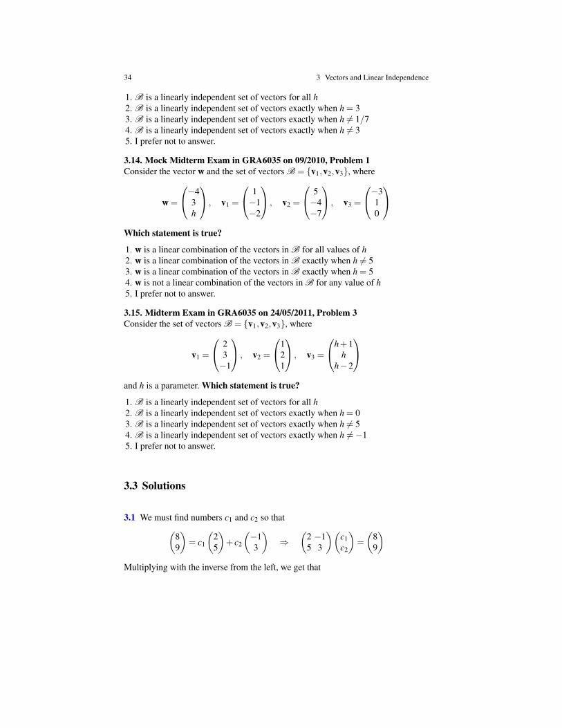
1. B is a linearly independent set of vectors for all h2. B is a linearly independent set of vectors exactly when h = 33. B is a linearly independent set of vectors exactly when h 6= 1/74. B is a linearly independent set of vectors exactly when h 6= 35. I prefer not to answer.
3.14. Mock Midterm Exam in GRA6035 on 09/2010, Problem 1Consider the vector w and the set of vectors B = {v1,v2,v3}, where
w =
−43h
, v1 =
1−1−2
, v2 =
5−4−7
, v3 =
−310
Which statement is true?
1. w is a linear combination of the vectors in B for all values of h2. w is a linear combination of the vectors in B exactly when h 6= 53. w is a linear combination of the vectors in B exactly when h = 54. w is not a linear combination of the vectors in B for any value of h5. I prefer not to answer.
3.15. Midterm Exam in GRA6035 on 24/05/2011, Problem 3Consider the set of vectors B = {v1,v2,v3}, where
v1 =
23−1
, v2 =
121
, v3 =
h+1h
h−2
and h is a parameter. Which statement is true?
1. B is a linearly independent set of vectors for all h2. B is a linearly independent set of vectors exactly when h = 03. B is a linearly independent set of vectors exactly when h 6= 54. B is a linearly independent set of vectors exactly when h 6=−15. I prefer not to answer.
3.3 Solutions
3.1 We must find numbers c1 and c2 so that(89
)= c1
(25
)+ c2
(−13
)⇒
(2 −15 3
)(c1c2
)=
(89
)Multiplying with the inverse from the left, we get that
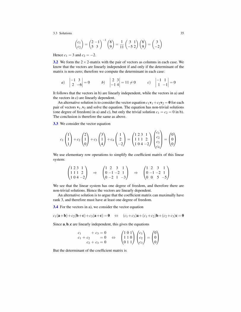
3.3 Solutions 35(c1c2
)=
(2 −15 3
)−1(89
)=
111
(3 1−5 2
)(89
)=
(3−2
)Hence c1 = 3 and c2 =−2.
3.2 We form the 2×2-matrix with the pair of vectors as columns in each case. Weknow that the vectors are linearly independent if and only if the determinant of thematrix is non-zero; therefore we compute the determinant in each case:
a)∣∣∣∣−1 3
2 −6
∣∣∣∣= 0 b)∣∣∣∣ 2 3−1 4
∣∣∣∣= 11 6= 0 c)∣∣∣∣−1 1
1 −1
∣∣∣∣= 0
It follows that the vectors in b) are linearly independent, while the vectors in a) andthe vectors in c) are linearly dependent.
An alternative solution is to consider the vector equation c1v1+c2v2 = 0 for eachpair of vectors v1,v2 and solve the equation. The equation has non-trivial solutions(one degree of freedom) in a) and c), but only the trivial solution c1 = c2 = 0 in b).The conclusion is therefore the same as above.
3.3 We consider the vector equation
c1
111
+ c2
210
+ c3
314
+ c4
12−2
=
1 2 3 11 1 1 21 0 4 −2
c1c2c3c4
=
000
We use elementary row operations to simplify the coefficient matrix of this linearsystem: 1 2 3 1
1 1 1 21 0 4 −2
⇒
1 2 3 10 −1 −2 10 −2 1 −3
⇒
1 2 3 10 −1 −2 10 0 5 −5
We see that the linear system has one degree of freedom, and therefore there arenon-trivial solutions. Hence the vectors are linearly dependent.
An alternative solution is to argue that the coefficient matrix can maximally haverank 3, and therefore must have at least one degree of freedom.
3.4 For the vectors in a), we consider the vector equation
c1(a+b)+c2(b+c)+c3(a+c) = 0 ⇔ (c1+c3)a+(c1+c2)b+(c2+c3)c= 0
Since a,b,c are linearly independent, this gives the equations
c1 + c3 = 0c1 + c2 = 0
c2 + c3 = 0⇔
1 0 11 1 00 1 1
c1c2c3
=
000
But the determinant of the coefficient matrix is
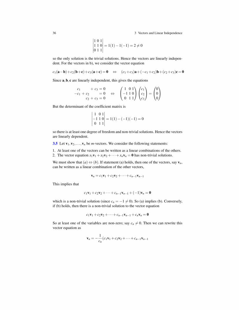
36 3 Vectors and Linear Independence∣∣∣∣∣∣1 0 11 1 00 1 1
∣∣∣∣∣∣= 1(1)−1(−1) = 2 6= 0
so the only solution is the trivial solutions. Hence the vectors are linearly indepen-dent. For the vectors in b), we consider the vector equation
c1(a−b)+c2(b+c)+c3(a+c)= 0 ⇔ (c1+c3)a+(−c1+c2)b+(c2+c3)c= 0
Since a,b,c are linearly independent, this gives the equations
c1 + c3 = 0−c1 + c2 = 0
c2 + c3 = 0⇔
1 0 1−1 1 00 1 1
c1c2c3
=
000
But the determinant of the coefficient matrix is∣∣∣∣∣∣
1 0 1−1 1 00 1 1
∣∣∣∣∣∣= 1(1)− (−1)(−1) = 0
so there is at least one degree of freedom and non-trivial solutions. Hence the vectorsare linearly dependent.
3.5 Let v1,v2, . . . ,vn be m-vectors. We consider the following statements:
1. At least one of the vectors can be written as a linear combinations of the others.2. The vector equation x1v1 + x2v2 + · · ·+ xnvn = 0 has non-trivial solutions.
We must show that (a)⇔ (b). If statement (a) holds, then one of the vectors, say vn,can be written as a linear combination of the other vectors,
vn = c1v1 + c2v2 + · · ·+ cn−1vn−1
This implies that
c1v1 + c2v2 + · · ·+ cn−1vn−1 +(−1)vn = 0
which is a non-trivial solution (since cn = −1 6= 0). So (a) implies (b). Conversely,if (b) holds, then there is a non-trivial solution to the vector equation
c1v1 + c2v2 + · · ·+ cn−1vn−1 + cnvn = 0
So at least one of the variables are non-zero; say cn 6= 0. Then we can rewrite thisvector equation as
vn =−1cn(c1v1 + c2v2 + · · ·+ cn−1vn−1
3.3 Solutions 37
Hence one of the vectors can be written as a linear combination of the others, and(b) implies (a).
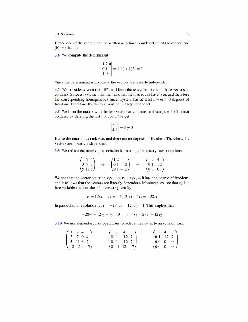
3.6 We compute the determinant∣∣∣∣∣∣1 2 00 1 11 0 1
∣∣∣∣∣∣= 1(1)+1(2) = 3
Since the determinant is non-zero, the vectors are linearly independent.
3.7 We consider n vectors in Rm, and form the m× n-matrix with these vectors ascolumns. Since n > m, the maximal rank that the matrix can have is m, and thereforethe corresponding homogeneous linear system has at least n−m > 0 degrees offreedom. Therefore, the vectors must be linearly dependent.
3.8 We form the matrix with the two vectors as columns, and compute the 2-minorobtained by deleting the last two rows. We get∣∣∣∣3 0
4 1
∣∣∣∣= 3 6= 0
Hence the matrix has rank two, and there are no degrees of freedom. Therefore, thevectors are linearly independent.
3.9 We reduce the matrix to an echelon form using elementary row operations:1 2 43 7 05 11 8
⇒
1 2 40 1 −120 1 −12
⇒
1 2 40 1 −120 0 0
We see that the vector equation x1v1 + x2v2 + x3v3 = 0 has one degree of freedom,and it follows that the vectors are linearly dependent. Moreover, we see that x3 is afree variable and that the solutions are given by
x2 = 12x3, x1 =−2(12x3)−4x3 =−28x3
In particular, one solution is x1 =−28, x2 = 12, x3 = 1. This implies that
−28v1 +12v2 +v3 = 0 ⇒ v3 = 28v1−12v2
3.10 We use elementary row operations to reduce the matrix to an echelon form:1 2 4 −13 7 0 45 11 8 2−2 −5 4 −5
⇒
1 2 4 −10 1 −12 70 1 −12 70 −1 12 −7
⇒
1 2 4 −10 1 −12 70 0 0 00 0 0 0
38 3 Vectors and Linear Independence
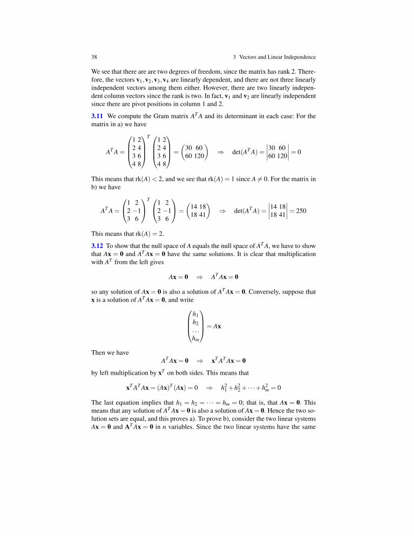
We see that there are are two degrees of freedom, since the matrix has rank 2. There-fore, the vectors v1,v2,v3,v4 are linearly dependent, and there are not three linearlyindependent vectors among them either. However, there are two linearly indepen-dent column vectors since the rank is two. In fact, v1 and v2 are linearly independentsince there are pivot positions in column 1 and 2.
3.11 We compute the Gram matrix AT A and its determinant in each case: For thematrix in a) we have
AT A =
1 22 43 64 8
T
1 22 43 64 8
=
(30 6060 120
)⇒ det(AT A) =
∣∣∣∣30 6060 120
∣∣∣∣= 0
This means that rk(A)< 2, and we see that rk(A) = 1 since A 6= 0. For the matrix inb) we have
AT A =
1 22 −13 6
T 1 22 −13 6
=
(14 1818 41
)⇒ det(AT A) =
∣∣∣∣14 1818 41
∣∣∣∣= 250
This means that rk(A) = 2.
3.12 To show that the null space of A equals the null space of AT A, we have to showthat Ax = 0 and AT Ax = 0 have the same solutions. It is clear that multiplicationwith AT from the left gives
Ax = 0 ⇒ AT Ax = 0
so any solution of Ax = 0 is also a solution of AT Ax = 0. Conversely, suppose thatx is a solution of AT Ax = 0, and write
h1h2. . .hm
= Ax
Then we haveAT Ax = 0 ⇒ xT AT Ax = 0
by left multiplication by xT on both sides. This means that
xT AT Ax = (Ax)T (Ax) = 0 ⇒ h21 +h2
2 + · · ·+h2m = 0
The last equation implies that h1 = h2 = · · · = hm = 0; that is, that Ax = 0. Thismeans that any solution of AT Ax = 0 is also a solution of Ax = 0. Hence the two so-lution sets are equal, and this proves a). To prove b), consider the two linear systemsAx = 0 and AT Ax = 0 in n variables. Since the two linear systems have the same
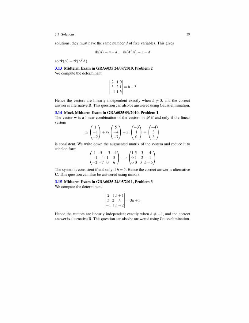
3.3 Solutions 39
solutions, they must have the same number d of free variables. This gives
rk(A) = n−d, rk(AT A) = n−d
so rk(A) = rk(AT A).
3.13 Midterm Exam in GRA6035 24/09/2010, Problem 2We compute the determinant ∣∣∣∣∣∣
2 1 03 2 1−1 1 h
∣∣∣∣∣∣= h−3
Hence the vectors are linearly independent exactly when h 6= 3, and the correctanswer is alternative D. This question can also be answered using Gauss elimination.
3.14 Mock Midterm Exam in GRA6035 09/2010, Problem 1The vector w is a linear combination of the vectors in B if and only if the linearsystem
x1
1−1−2
+ x2
5−4−7
+ x3
−310
=
−43h
is consistent. We write down the augmented matrix of the system and reduce it toechelon form 1 5 −3 −4
−1 −4 1 3−2 −7 0 h
99K
1 5 −3 −40 1 −2 −10 0 0 h−5
The system is consistent if and only if h = 5. Hence the correct answer is alternativeC. This question can also be answered using minors.
3.15 Midterm Exam in GRA6035 24/05/2011, Problem 3We compute the determinant ∣∣∣∣∣∣
2 1 h+13 2 h−1 1 h−2
∣∣∣∣∣∣= 3h+3
Hence the vectors are linearly independent exactly when h 6= −1, and the correctanswer is alternative D. This question can also be answered using Gauss elimination.

Previous: Lecture 3 Contents Next: Lecture 5
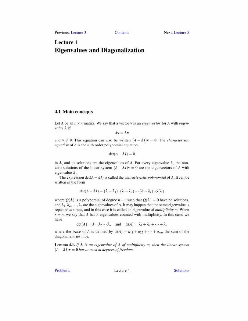
Lecture 4Eigenvalues and Diagonalization
4.1 Main concepts
Let A be an n×n matrix. We say that a vector v is an eigenvector for A with eigen-value λ if
Av = λv
and v 6= 0. This equation can also be written (A− λ I)v = 0. The characteristicequation of A is the n’th order polynomial equation
det(A−λ I) = 0
in λ , and its solutions are the eigenvalues of A. For every eigenvalue λ , the non-zero solutions of the linear system (A− λ I)v = 0 are the eigenvectors of A witheigenvalue λ .
The expression det(A−λ I) is called the characteristic polynomial of A. It can bewritten in the form
det(A−λ I) = (λ −λ1) · (λ −λ2) · · ·(λ −λr) ·Q(λ )
where Q(λ ) is a polynomial of degree n− r such that Q(λ ) = 0 have no solutions,and λ1,λ2, . . . ,λr are the eigenvalues of A. It may happen that the same eigenvalue isrepeated m times, and in this case it is called an eigenvalue of multiplicity m. Whenr = n, we say that A has n eigenvalues counted with multiplicity. In this case, wehave
det(A) = λ1 ·λ2 · · ·λn and tr(A) = λ1 +λ2 + · · ·+λn
where the trace of A is defined by tr(A) = a11 + a22 + · · ·+ ann, the sum of thediagonal entries in A.
Lemma 4.1. If λ is an eigenvalue of A of multiplicity m, then the linear system(A−λ I)v = 0 has at most m degrees of freedom.
Problems Lecture 4 Solutions
42 4 Eigenvalues and Diagonalization
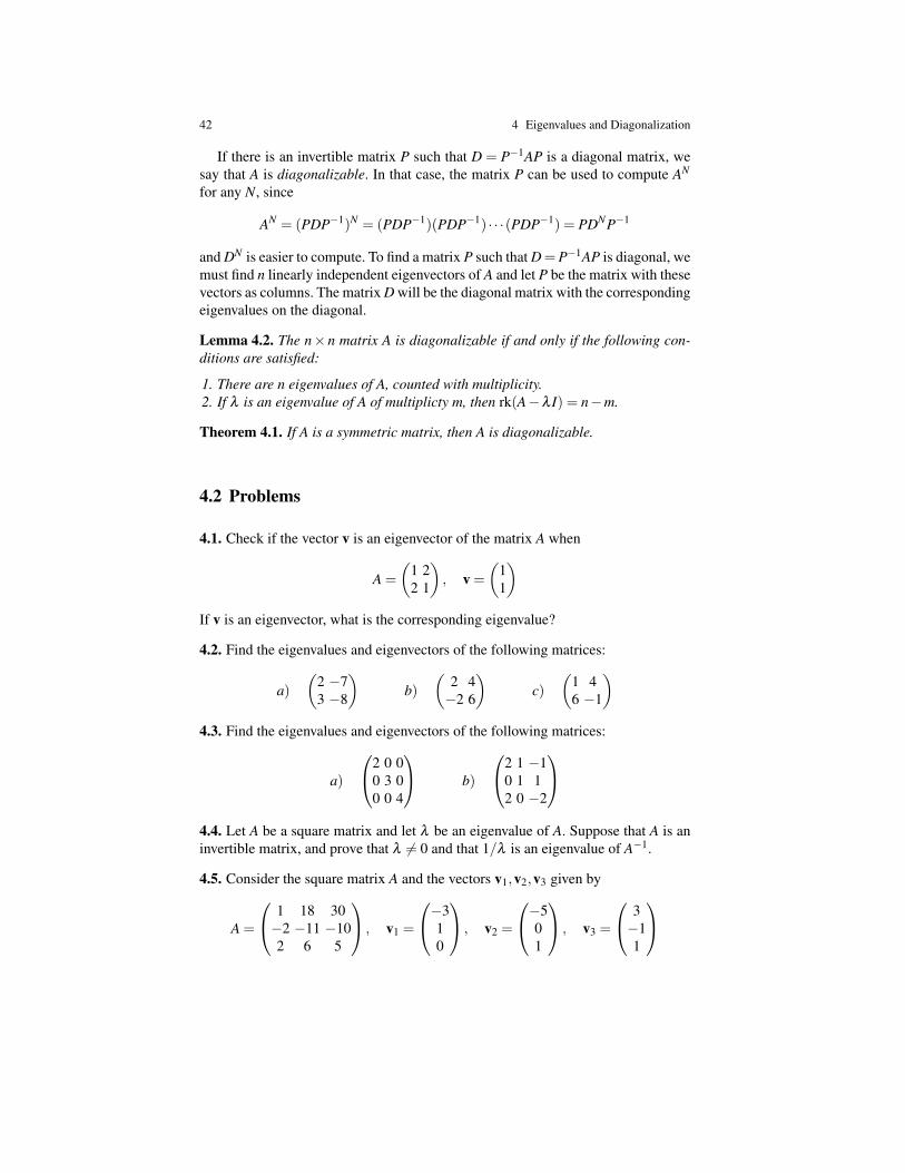
If there is an invertible matrix P such that D = P−1AP is a diagonal matrix, wesay that A is diagonalizable. In that case, the matrix P can be used to compute AN
for any N, since
AN = (PDP−1)N = (PDP−1)(PDP−1) · · ·(PDP−1) = PDNP−1
and DN is easier to compute. To find a matrix P such that D=P−1AP is diagonal, wemust find n linearly independent eigenvectors of A and let P be the matrix with thesevectors as columns. The matrix D will be the diagonal matrix with the correspondingeigenvalues on the diagonal.
Lemma 4.2. The n× n matrix A is diagonalizable if and only if the following con-ditions are satisfied:
1. There are n eigenvalues of A, counted with multiplicity.2. If λ is an eigenvalue of A of multiplicty m, then rk(A−λ I) = n−m.
Theorem 4.1. If A is a symmetric matrix, then A is diagonalizable.
4.2 Problems
4.1. Check if the vector v is an eigenvector of the matrix A when
A =
(1 22 1
), v =
(11
)If v is an eigenvector, what is the corresponding eigenvalue?
4.2. Find the eigenvalues and eigenvectors of the following matrices:
a)(
2 −73 −8
)b)
(2 4−2 6
)c)
(1 46 −1
)4.3. Find the eigenvalues and eigenvectors of the following matrices:
a)
2 0 00 3 00 0 4
b)
2 1 −10 1 12 0 −2
4.4. Let A be a square matrix and let λ be an eigenvalue of A. Suppose that A is aninvertible matrix, and prove that λ 6= 0 and that 1/λ is an eigenvalue of A−1.
4.5. Consider the square matrix A and the vectors v1,v2,v3 given by
A =
1 18 30−2 −11 −102 6 5
, v1 =
−310
, v2 =
−501
, v3 =
3−11
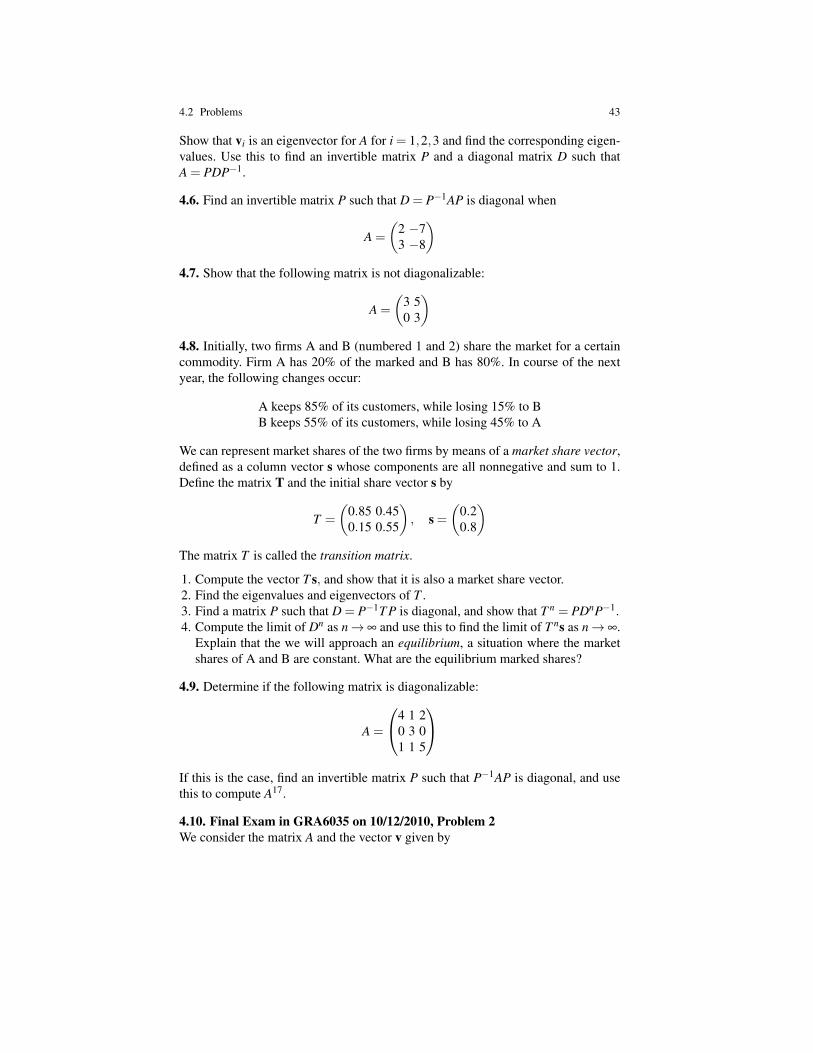
4.2 Problems 43
Show that vi is an eigenvector for A for i = 1,2,3 and find the corresponding eigen-values. Use this to find an invertible matrix P and a diagonal matrix D such thatA = PDP−1.
4.6. Find an invertible matrix P such that D = P−1AP is diagonal when
A =
(2 −73 −8
)4.7. Show that the following matrix is not diagonalizable:
A =
(3 50 3
)4.8. Initially, two firms A and B (numbered 1 and 2) share the market for a certaincommodity. Firm A has 20% of the marked and B has 80%. In course of the nextyear, the following changes occur:
A keeps 85% of its customers, while losing 15% to BB keeps 55% of its customers, while losing 45% to A
We can represent market shares of the two firms by means of a market share vector,defined as a column vector s whose components are all nonnegative and sum to 1.Define the matrix T and the initial share vector s by
T =
(0.85 0.450.15 0.55
), s =
(0.20.8
)The matrix T is called the transition matrix.
1. Compute the vector T s, and show that it is also a market share vector.2. Find the eigenvalues and eigenvectors of T .3. Find a matrix P such that D = P−1T P is diagonal, and show that T n = PDnP−1.4. Compute the limit of Dn as n→ ∞ and use this to find the limit of T ns as n→ ∞.
Explain that the we will approach an equilibrium, a situation where the marketshares of A and B are constant. What are the equilibrium marked shares?
4.9. Determine if the following matrix is diagonalizable:
A =
4 1 20 3 01 1 5
If this is the case, find an invertible matrix P such that P−1AP is diagonal, and usethis to compute A17.
4.10. Final Exam in GRA6035 on 10/12/2010, Problem 2We consider the matrix A and the vector v given by
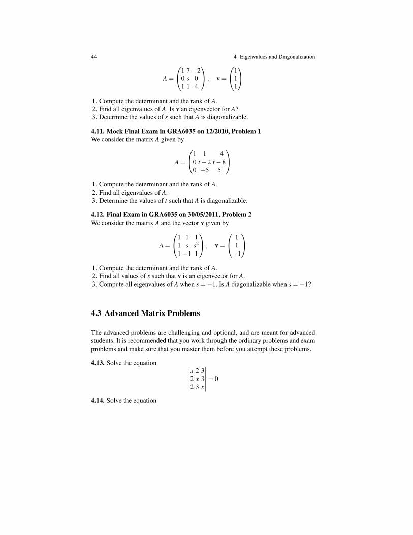
44 4 Eigenvalues and Diagonalization
A =
1 7 −20 s 01 1 4
, v =
111
1. Compute the determinant and the rank of A.2. Find all eigenvalues of A. Is v an eigenvector for A?3. Determine the values of s such that A is diagonalizable.
4.11. Mock Final Exam in GRA6035 on 12/2010, Problem 1We consider the matrix A given by
A =
1 1 −40 t +2 t−80 −5 5
1. Compute the determinant and the rank of A.2. Find all eigenvalues of A.3. Determine the values of t such that A is diagonalizable.
4.12. Final Exam in GRA6035 on 30/05/2011, Problem 2We consider the matrix A and the vector v given by
A =
1 1 11 s s2
1 −1 1
, v =
11−1
1. Compute the determinant and the rank of A.2. Find all values of s such that v is an eigenvector for A.3. Compute all eigenvalues of A when s =−1. Is A diagonalizable when s =−1?
4.3 Advanced Matrix Problems
The advanced problems are challenging and optional, and are meant for advancedstudents. It is recommended that you work through the ordinary problems and examproblems and make sure that you master them before you attempt these problems.
4.13. Solve the equation ∣∣∣∣∣∣x 2 32 x 32 3 x
∣∣∣∣∣∣= 0
4.14. Solve the equation
4.4 Solutions 45∣∣∣∣∣∣∣∣∣∣∣∣
x+1 0 x 0 x−1 00 x 0 x−1 0 x+1x 0 x−1 0 x+1 00 x−1 0 x+1 0 x
x−1 0 x+1 0 x 00 x+1 0 x 0 x−1
∣∣∣∣∣∣∣∣∣∣∣∣= 9
4.15. Solve the linear system
x2 + x3 + . . . + xn−1 + xn = 2x1 + x3 + . . . + xn−1 + xn = 4x1 + x2 + . . . + xn−1 + xn = 6
......
x1 + x2 + x3 + . . . + xn−1 = 2n
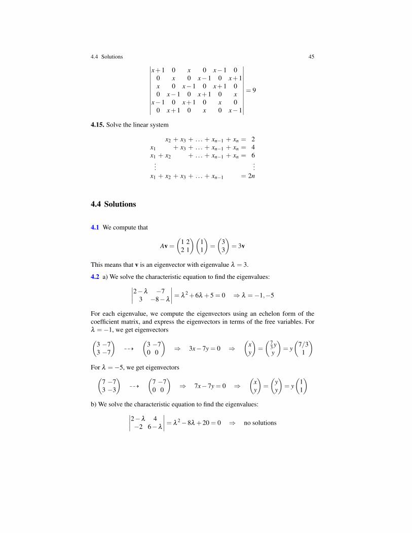
4.4 Solutions
4.1 We compute that
Av =
(1 22 1
)(11
)=
(33
)= 3v
This means that v is an eigenvector with eigenvalue λ = 3.
4.2 a) We solve the characteristic equation to find the eigenvalues:∣∣∣∣2−λ −73 −8−λ
∣∣∣∣= λ2 +6λ +5 = 0 ⇒ λ =−1,−5
For each eigenvalue, we compute the eigenvectors using an echelon form of thecoefficient matrix, and express the eigenvectors in terms of the free variables. Forλ =−1, we get eigenvectors(
3 −73 −7
)99K
(3 −70 0
)⇒ 3x−7y = 0 ⇒
(xy
)=
( 73 yy
)= y(
7/31
)For λ =−5, we get eigenvectors(
7 −73 −3
)99K
(7 −70 0
)⇒ 7x−7y = 0 ⇒
(xy
)=
(yy
)= y(
11
)b) We solve the characteristic equation to find the eigenvalues:∣∣∣∣2−λ 4
−2 6−λ
∣∣∣∣= λ2−8λ +20 = 0 ⇒ no solutions
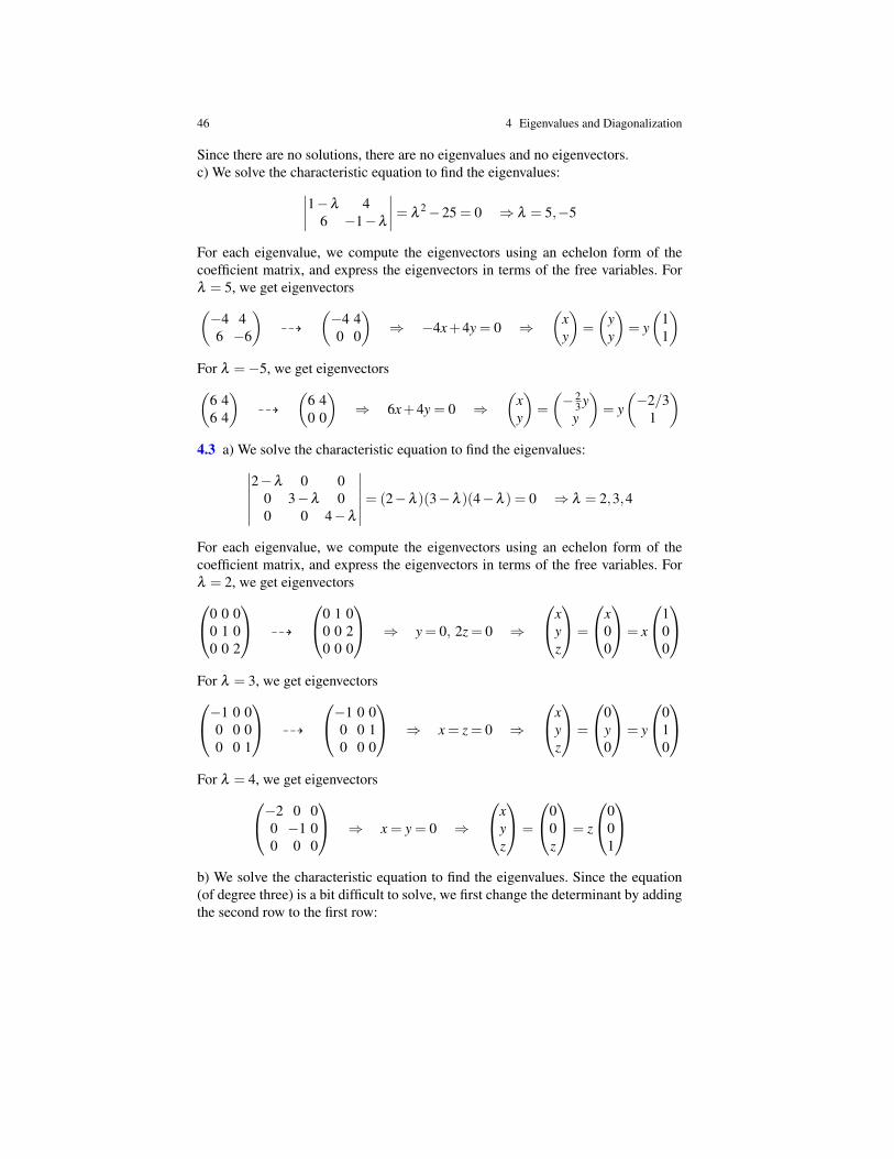
46 4 Eigenvalues and Diagonalization
Since there are no solutions, there are no eigenvalues and no eigenvectors.c) We solve the characteristic equation to find the eigenvalues:∣∣∣∣1−λ 4
6 −1−λ
∣∣∣∣= λ2−25 = 0 ⇒ λ = 5,−5
For each eigenvalue, we compute the eigenvectors using an echelon form of thecoefficient matrix, and express the eigenvectors in terms of the free variables. Forλ = 5, we get eigenvectors(−4 46 −6
)99K
(−4 40 0
)⇒ −4x+4y = 0 ⇒
(xy
)=
(yy
)= y(
11
)For λ =−5, we get eigenvectors(
6 46 4
)99K
(6 40 0
)⇒ 6x+4y = 0 ⇒
(xy
)=
(− 2
3 yy
)= y(−2/3
1
)4.3 a) We solve the characteristic equation to find the eigenvalues:∣∣∣∣∣∣
2−λ 0 00 3−λ 00 0 4−λ
∣∣∣∣∣∣= (2−λ )(3−λ )(4−λ ) = 0 ⇒ λ = 2,3,4
For each eigenvalue, we compute the eigenvectors using an echelon form of thecoefficient matrix, and express the eigenvectors in terms of the free variables. Forλ = 2, we get eigenvectors0 0 0
0 1 00 0 2
99K
0 1 00 0 20 0 0
⇒ y = 0, 2z = 0 ⇒
xyz
=
x00
= x
100
For λ = 3, we get eigenvectors−1 0 0
0 0 00 0 1
99K
−1 0 00 0 10 0 0
⇒ x = z = 0 ⇒
xyz
=
0y0
= y
010
For λ = 4, we get eigenvectors−2 0 0
0 −1 00 0 0
⇒ x = y = 0 ⇒
xyz
=
00z
= z
001
b) We solve the characteristic equation to find the eigenvalues. Since the equation(of degree three) is a bit difficult to solve, we first change the determinant by addingthe second row to the first row:
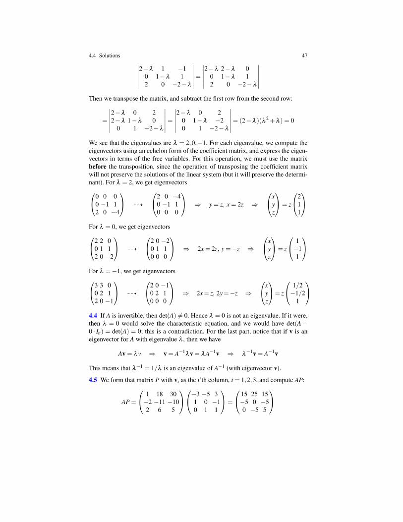
4.4 Solutions 47∣∣∣∣∣∣2−λ 1 −1
0 1−λ 12 0 −2−λ
∣∣∣∣∣∣=∣∣∣∣∣∣2−λ 2−λ 0
0 1−λ 12 0 −2−λ
∣∣∣∣∣∣Then we transpose the matrix, and subtract the first row from the second row:
=
∣∣∣∣∣∣2−λ 0 22−λ 1−λ 0
0 1 −2−λ
∣∣∣∣∣∣=∣∣∣∣∣∣2−λ 0 2
0 1−λ −20 1 −2−λ
∣∣∣∣∣∣= (2−λ )(λ 2 +λ ) = 0
We see that the eigenvalues are λ = 2,0,−1. For each eigenvalue, we compute theeigenvectors using an echelon form of the coefficient matrix, and express the eigen-vectors in terms of the free variables. For this operation, we must use the matrixbefore the transposition, since the operation of transposing the coefficient matrixwill not preserve the solutions of the linear system (but it will preserve the determi-nant). For λ = 2, we get eigenvectors0 0 0
0 −1 12 0 −4
99K
2 0 −40 −1 10 0 0
⇒ y = z, x = 2z ⇒
xyz
= z
211
For λ = 0, we get eigenvectors2 2 0
0 1 12 0 −2
99K
2 0 −20 1 10 0 0
⇒ 2x = 2z, y =−z ⇒
xyz
= z
1−11
For λ =−1, we get eigenvectors3 3 0
0 2 12 0 −1
99K
2 0 −10 2 10 0 0
⇒ 2x= z, 2y=−z ⇒
xyz
= z
1/2−1/2
1
4.4 If A is invertible, then det(A) 6= 0. Hence λ = 0 is not an eigenvalue. If it were,then λ = 0 would solve the characteristic equation, and we would have det(A−0 · In) = det(A) = 0; this is a contradiction. For the last part, notice that if v is aneigenvector for A with eigenvalue λ , then we have
Av = λv ⇒ v = A−1λv = λA−1v ⇒ λ
−1v = A−1v
This means that λ−1 = 1/λ is an eigenvalue of A−1 (with eigenvector v).
4.5 We form that matrix P with vi as the i’th column, i = 1,2,3, and compute AP:
AP =
1 18 30−2 −11 −102 6 5
−3 −5 31 0 −10 1 1
=
15 25 15−5 0 −50 −5 5
48 4 Eigenvalues and Diagonalization
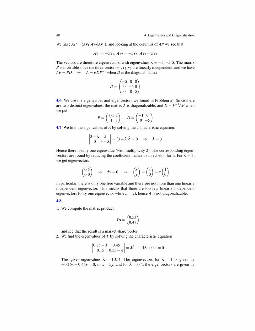
We have AP = (Av1|Av2|Av3), and looking at the columns of AP we see that
Av1 =−5v1, Av2 =−5v2, Av3 = 5v3
The vectors are therefore eigenvectors, with eigenvalues λ =−5,−5,5. The matrixP is invertible since the three vectors v1,v2,v3 are linearly independent, and we haveAP = PD ⇒ A = PDP−1 when D is the diagonal matrix
D =
−5 0 00 −5 00 0 5
4.6 We use the eigenvalues and eigenvectors we found in Problem a). Since thereare two distinct eigenvalues, the matrix A is diagonalizable, and D = P−1AP whenwe put
P =
(7/3 11 1
), D =
(−1 00 −5
)4.7 We find the eigenvalues of A by solving the characteristic equation:∣∣∣∣3−λ 5
0 3−λ
∣∣∣∣= (3−λ )2 = 0 ⇒ λ = 3
Hence there is only one eigenvalue (with multiplicity 2). The corresponding eigen-vectors are found by reducing the coefficient matrix to an echelon form. For λ = 3,we get eigenvectors(
0 50 0
)⇒ 5y = 0 ⇒
(xy
)=
(x0
)= x(
10
)In particular, there is only one free variable and therefore not more than one linearlyindependent eigenvector. This means that there are too few linearly independenteigenvectors (only one eigenvector while n = 2), hence A is not diagonalizable.
4.8
1. We compute the matrix product
T s =(
0.530.47
)and see that the result is a market share vector.
2. We find the eigenvalues of T by solving the characteristic equation∣∣∣∣0.85−λ 0.450.15 0.55−λ
∣∣∣∣= λ2−1.4λ +0.4 = 0
This gives eigenvalues λ = 1,0.4. The eigenvectors for λ = 1 is given by−0.15x+ 0.45y = 0, or x = 3y; and for λ = 0.4, the eigenvectors are given by
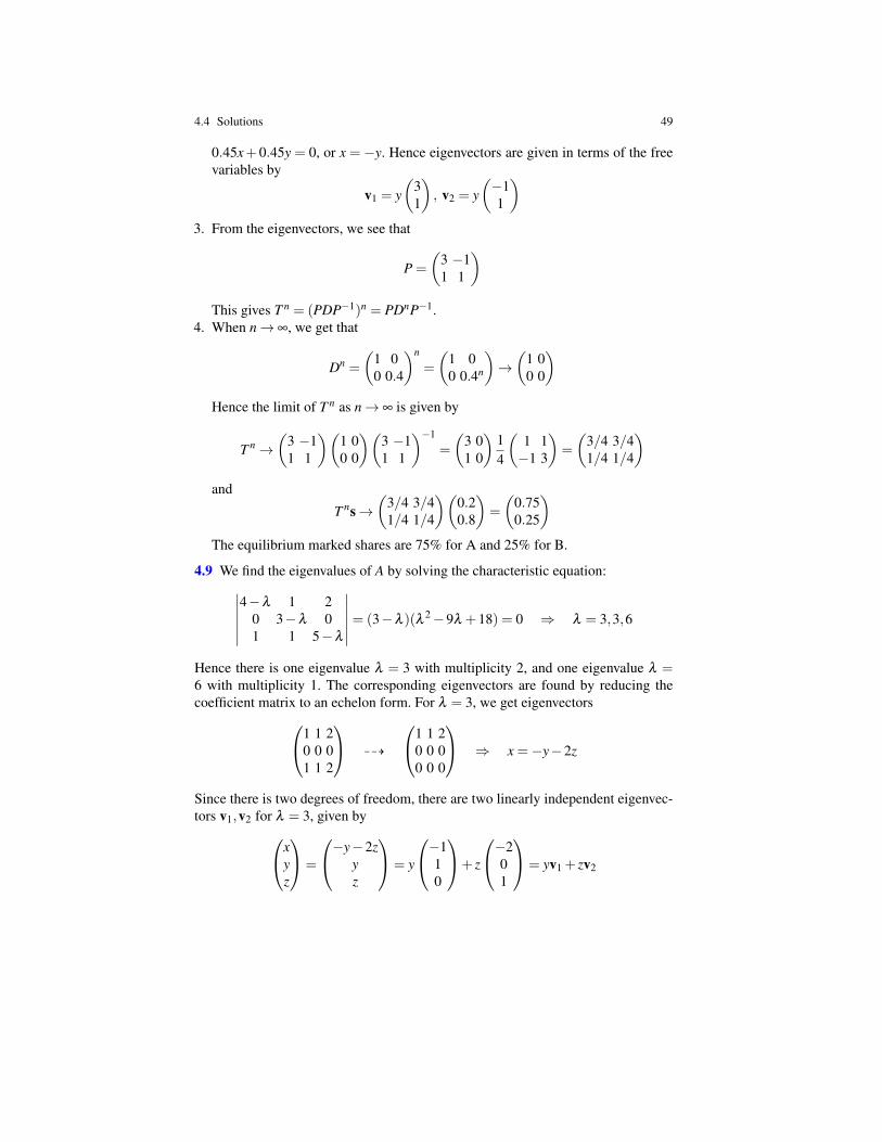
4.4 Solutions 49
0.45x+0.45y = 0, or x = −y. Hence eigenvectors are given in terms of the freevariables by
v1 = y(
31
), v2 = y
(−11
)3. From the eigenvectors, we see that
P =
(3 −11 1
)This gives T n = (PDP−1)n = PDnP−1.
4. When n→ ∞, we get that
Dn =
(1 00 0.4
)n
=
(1 00 0.4n
)→(
1 00 0
)Hence the limit of T n as n→ ∞ is given by
T n→(
3 −11 1
)(1 00 0
)(3 −11 1
)−1
=
(3 01 0
)14
(1 1−1 3
)=
(3/4 3/41/4 1/4
)and
T ns→(
3/4 3/41/4 1/4
)(0.20.8
)=
(0.750.25
)The equilibrium marked shares are 75% for A and 25% for B.
4.9 We find the eigenvalues of A by solving the characteristic equation:∣∣∣∣∣∣4−λ 1 2
0 3−λ 01 1 5−λ
∣∣∣∣∣∣= (3−λ )(λ 2−9λ +18) = 0 ⇒ λ = 3,3,6
Hence there is one eigenvalue λ = 3 with multiplicity 2, and one eigenvalue λ =6 with multiplicity 1. The corresponding eigenvectors are found by reducing thecoefficient matrix to an echelon form. For λ = 3, we get eigenvectors1 1 2
0 0 01 1 2
99K
1 1 20 0 00 0 0
⇒ x =−y−2z
Since there is two degrees of freedom, there are two linearly independent eigenvec-tors v1,v2 for λ = 3, given byx
yz
=
−y−2zyz
= y
−110
+ z
−201
= yv1 + zv2
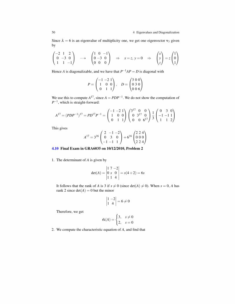
50 4 Eigenvalues and Diagonalization
Since λ = 6 is an eigenvalue of multiplicity one, we get one eigenvector v3 givenby−2 1 2
0 −3 01 1 −1
99K
1 0 −10 −3 00 0 0
⇒ x = z, y = 0 ⇒
xyz
= z
101
Hence A is diagonalizable, and we have that P−1AP = D is diagonal with
P =
−1 −2 11 0 00 1 1
, D =
3 0 00 3 00 0 6
We use this to compute A17, since A = PDP−1. We do not show the computation ofP−1, which is straight-forward:
A17 = (PDP−1)17 = PD17P−1 =
−1 −2 11 0 00 1 1
317 0 00 317 00 0 617
13
0 3 0−1 −1 11 1 2
This gives
A17 = 316
2 −1 −20 3 0−1 −1 1
+616
2 2 40 0 02 2 4
4.10 Final Exam in GRA6035 on 10/12/2010, Problem 2
1. The determinant of A is given by
det(A) =
∣∣∣∣∣∣1 7 −20 s 01 1 4
∣∣∣∣∣∣= s(4+2) = 6s
It follows that the rank of A is 3 if s 6= 0 (since det(A) 6= 0). When s = 0, A hasrank 2 since det(A) = 0 but the minor∣∣∣∣1 −2
1 4
∣∣∣∣= 6 6= 0
Therefore, we get
rk(A) =
{3, s 6= 02, s = 0
2. We compute the characteristic equation of A, and find that
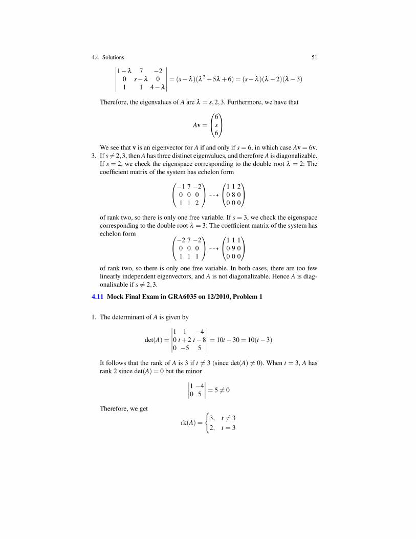
4.4 Solutions 51∣∣∣∣∣∣1−λ 7 −2
0 s−λ 01 1 4−λ
∣∣∣∣∣∣= (s−λ )(λ 2−5λ +6) = (s−λ )(λ −2)(λ −3)
Therefore, the eigenvalues of A are λ = s,2,3. Furthermore, we have that
Av =
6s6
We see that v is an eigenvector for A if and only if s = 6, in which case Av = 6v.
3. If s 6= 2,3, then A has three distinct eigenvalues, and therefore A is diagonalizable.If s = 2, we check the eigenspace corresponding to the double root λ = 2: Thecoefficient matrix of the system has echelon form−1 7 −2
0 0 01 1 2
99K
1 1 20 8 00 0 0
of rank two, so there is only one free variable. If s = 3, we check the eigenspacecorresponding to the double root λ = 3: The coefficient matrix of the system hasechelon form −2 7 −2
0 0 01 1 1
99K
1 1 10 9 00 0 0
of rank two, so there is only one free variable. In both cases, there are too fewlinearly independent eigenvectors, and A is not diagonalizable. Hence A is diag-onalixable if s 6= 2,3.
4.11 Mock Final Exam in GRA6035 on 12/2010, Problem 1
1. The determinant of A is given by
det(A) =
∣∣∣∣∣∣1 1 −40 t +2 t−80 −5 5
∣∣∣∣∣∣= 10t−30 = 10(t−3)
It follows that the rank of A is 3 if t 6= 3 (since det(A) 6= 0). When t = 3, A hasrank 2 since det(A) = 0 but the minor∣∣∣∣1 −4
0 5
∣∣∣∣= 5 6= 0
Therefore, we get
rk(A) =
{3, t 6= 32, t = 3
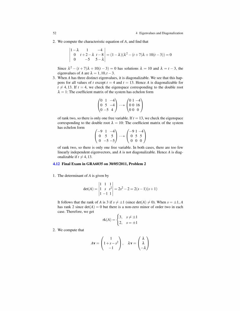
52 4 Eigenvalues and Diagonalization
2. We compute the characteristic equation of A, and find that∣∣∣∣∣∣1−λ 1 −4
0 t +2−λ t−80 −5 5−λ
∣∣∣∣∣∣= (1−λ )(λ 2− (t +7)λ +10(t−3)) = 0
Since λ 2 − (t + 7)λ + 10(t − 3) = 0 has solutions λ = 10 and λ = t − 3, theeigenvalues of A are λ = 1,10, t−3.
3. When A has three distinct eigenvalues, it is diagonalizable. We see that this hap-pens for all values of t except t = 4 and t = 13. Hence A is diagonalizable fort 6= 4,13. If t = 4, we check the eigenspace corresponding to the double rootλ = 1: The coefficient matrix of the system has echelon form0 1 −4
0 5 −40 −5 4
99K
0 1 −40 0 160 0 0
of rank two, so there is only one free variable. If t = 13, we check the eigenspacecorresponding to the double root λ = 10: The coefficient matrix of the systemhas echelon form −9 1 −4
0 5 50 −5 −5
99K
−9 1 −40 5 50 0 0
of rank two, so there is only one free variable. In both cases, there are too fewlinearly independent eigenvectors, and A is not diagonalizable. Hence A is diag-onalizable if t 6= 4,13.
4.12 Final Exam in GRA6035 on 30/05/2011, Problem 2
1. The determinant of A is given by
det(A) =
∣∣∣∣∣∣1 1 11 s s2
1 −1 1
∣∣∣∣∣∣= 2s2−2 = 2(s−1)(s+1)
It follows that the rank of A is 3 if s 6= ±1 (since det(A) 6= 0). When s = ±1, Ahas rank 2 since det(A) = 0 but there is a non-zero minor of order two in eachcase. Therefore, we get
rk(A) =
{3, s 6=±12, s =±1
2. We compute that
Av =
11+ s− s2
−1
, λv =
λ
λ
−λ
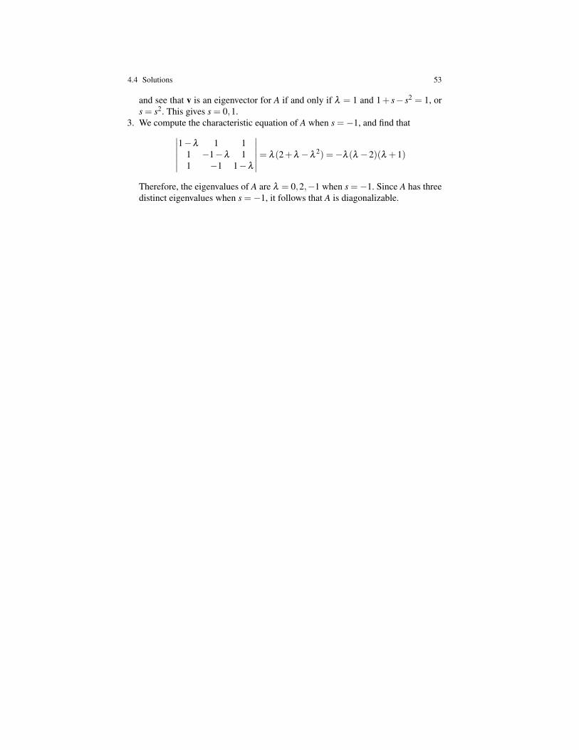
4.4 Solutions 53
and see that v is an eigenvector for A if and only if λ = 1 and 1+ s− s2 = 1, ors = s2. This gives s = 0,1.
3. We compute the characteristic equation of A when s =−1, and find that∣∣∣∣∣∣1−λ 1 1
1 −1−λ 11 −1 1−λ
∣∣∣∣∣∣= λ (2+λ −λ2) =−λ (λ −2)(λ +1)
Therefore, the eigenvalues of A are λ = 0,2,−1 when s =−1. Since A has threedistinct eigenvalues when s =−1, it follows that A is diagonalizable.

Previous: Lecture 4 Contents Next: Lecture 6
Lecture 5Quadratic Forms and Definiteness
5.1 Main concepts
A Markov process or a Markov chain is a model for a system that at any time can bedescribed by a state vector x = xt , which is an n-vector with x1,x2, . . . ,xn ≥ 0 andx1 + · · ·+xn = 1. The defining property of a Markov chain is that there is a constantn× n-matrix A = (ai j), called the transition matrix, with ai j ≥ 0 and where eachcolumn sums to 1, such that
xt+1 = Axt for t = 1,2,3, . . .
If ai j > 0 for all i, j, the Markov chain is called regular. In that case, we have that
1. λ = 1 is an eigenvalue of A with multiplicity 12. There is a unique eigenvector v with eigenvalue 1 that is also a state vector3. For any initial state x0, we have that
limt→∞
xt = limt→∞
Atx0 = v
The state v is called the equilibrium state of the process.A quadratic form is a polynomial function f (x1,x2, . . . ,xn) = f (x) where all
terms have degree two. It has the form
f (x) = c11 x21 + c12 x1x2 + · · ·+ cnn x2
n
where ci j are given numbers. There is a unique symmetric n× n matrix A, calledthe symmetric matrix of the quadratic form, such that f (x) = xT Ax. This matrix isgiven by
A = (ai j), where aii = cii and ai j = a ji = ci j/2 for i 6= j
The quadratic form f , and the symmetric matrix A, is called
1. positive definite if f (x)> 0 for all x 6= 0
Problems Lecture 5 Solutions
56 5 Quadratic Forms and Definiteness
2. negative definite if f (x)< 0 for all x 6= 03. positive semidefinite if f (x)≥ 0 for all x4. negative semidefinite if f (x)≤ 0 for all x5. indefinite if f takes both positive and negative values
If f is positive definite, then x = 0 is a global minimum for f , and if f is negativedefinite, then x = 0 is a global maximum for f .
Proposition 5.1. Let f be a quadratic form with symmetric matrix A, and letλ1, . . .λn be the eigenvalues of A.
1. A is positive definite if and only if λ1, . . . ,λn > 02. A is negative definite if and only if λ1, . . . ,λn < 03. A is positive semidefinite if and only if λ1, . . . ,λn ≥ 04. A is negative semidefinite if and only if λ1, . . . ,λn ≤ 05. A is indefinite if and only if it has both positive and negative eigenvalues
Let A be a symmetric n× n matrix. The leading principal minor Di of order iis the minor obtained by keeping the first i rows and columns of A, and deletingthe remaining rows and columns. A principal minor of order i is a minor of orderi obtained by deleting n− i rows and the n− i columns with the same numbering.There are in general many principal minors of order i, and we denote any one ofthem by ∆i.
Proposition 5.2. Let f be a quadratic form with symmetric matrix A.
1. A is positive definite if and only if D1,D2, . . . ,Dn > 02. A is negative definite if and only if Di < 0 when i is odd and Di > 0 when i is even3. A is positive semidefinite if and only if ∆i ≥ 0 for any principal minor ∆i4. A is negative semidefinite if and only if ∆i ≤ 0 for any principal minor of odd
order i and ∆i ≥ 0 for any principal minor of even order i
5.2 Problems
5.1. Find the symmetric matrix of the following quadratic forms:
1. Q(x,y) = x2 +2xy+ y2
2. Q(x,y) = ax2 +bxy+ cy2
3. Q(x,y,z) = 3x2−2xy+3xz+2y2 +3z2
5.2. Find the symmetric matrix and determine the definiteness of the followingquadratic forms:
1. Q(x) = x21 +3x2
2 +5x23
2. Q(x) = x21 +2x1x2 +3x2
2 +5x23
5.2 Problems 57
5.3. Compute all leading principal minors and all principal minors of the followingmatrices:
a) A =
(−3 44 −5
)b) A =
(−3 44 −6
)In each case, write down the corresponding quadratic form Q(x,y) = xT Ax, anddetermine its definiteness. Use this to classify the stationary point (x,y) = (0,0) ofthe quadratic form.
5.4. Compute all leading principal minors and all principal minors of the matrix
A =
1 2 02 4 50 5 6
Write down the corresponding quadratic form Q(x,y,z) = xT Ax, and determineits definiteness. Use this to classify the stationary point (x,y,z) = (0,0,0) of thequadratic form.
5.5. For which values of the parameters a,b,c is the symmetric matrix(a bb c
)positive (semi)definite and negative (semi)definite?
5.6. Determine the definiteness of the following quadratic forms:
1. f (x,y) = 2x2−2xy+ y2
2. f (x,y) =−3x2 +8xy−5y2
3. f (x,y) =−3x2 +8xy−6y2
4. f (x,y) = 2x2 +8xy+8y2
5. f (x,y,z) = x2 +4xy+4y2 +10yz+6z2
6. f (x,y,z) =−x2 +2xy− y2−2z2
7. f (x,y,z,w) = x2 +6xz+2y2 +10yw+4z2 +6w2
5.7. Give a detailed proof that AT A is positive definite for any invertible matrix A.
5.8. Find the equilibrium state x of a Markov chain xt+1 =Axt with transition matrix
A =
(0.87 0.160.13 0.84
)5.9. Find the equilibrium state x of a Markov chain xt+1 =Axt with transition matrix
A =
0.61 0.13 0.030.13 0.81 0.100.26 0.06 0.87
58 5 Quadratic Forms and Definiteness
5.10. Midterm in GRA6035 24/09/2010, Problem 6Consider the quadratic form
Q(x1,x2) = x21−4x1x2 +4x2
2
Which statement is true?
1. Q is positive semidefinite but not positive definite2. Q is negative semidefinite but not negative definite3. Q is indefinite4. Q is positive definite5. I prefer not to answer.
5.11. Mock Midterm in GRA6035 09/2010, Problem 6Consider the function
f (x1,x2,x3) = x21 +6x1x2 +3x2
2 +2x23
Which statement is true?
1. f is not a quadratic form2. f is a positive definite quadratic form3. f is an indefinite quadratic form4. f is a negative definite quadratic form5. I prefer not to answer.
5.12. Midterm in GRA6035 24/05/2011, Problem 6Consider the quadratic form
Q(x1,x2) =−2x21 +12x1x2 +2x2
2
Which statement is true?
1. Q is positive semidefinite but not positive definite2. Q is negative semidefinite but not negative definite3. Q is indefinite4. Q is positive definite5. I prefer not to answer.
5.13. Final exam in GRA6035 12/12/2014, Problem 2We consider the matrix A given by
A =
t 1 11 t 11 1 t
1. Compute the determinant of A, and the rank of A−λ I when λ = t−1.2. Show that A is diagonalizable when t = 8, and find all its eigenvalues in this case.
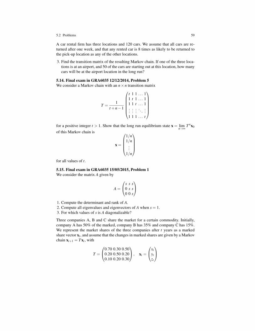
5.2 Problems 59
A car rental firm has three locations and 120 cars. We assume that all cars are re-turned after one week, and that any rented car is 8 times as likely to be returned tothe pick-up location as any of the other locations.
3. Find the transition matrix of the resulting Markov chain. If one of the three loca-tions is at an airport, and 50 of the cars are starting out at this location, how manycars will be at the airport location in the long run?
5.14. Final exam in GRA6035 12/12/2014, Problem 5We consider a Markov chain with an n×n transition matrix
T =1
t +n−1
t 1 1 . . . 11 t 1 . . . 11 1 t . . . 1...
......
. . ....
1 1 1 . . . t
for a positive integer t > 1. Show that the long run equilibrium state x = lim
n→∞T nx0
of this Markov chain is
x =
1/n1/n
...1/n
for all values of t.
5.15. Final exam in GRA6035 15/05/2015, Problem 1We consider the matrix A given by
A =
s s s0 s s0 0 s
1. Compute the determinant and rank of A.2. Compute all eigenvalues and eigenvectors of A when s = 1.3. For which values of s is A diagonalizable?
Three companies A, B and C share the market for a certain commodity. Initially,company A has 50% of the marked, company B has 35% and company C has 15%.We represent the market shares of the three companies after t years as a markedshare vector xt , and assume that the changes in marked shares are given by a Markovchain xt+1 = T xt , with
T =
0.70 0.30 0.500.20 0.50 0.200.10 0.20 0.30
, xt =
xtytzt
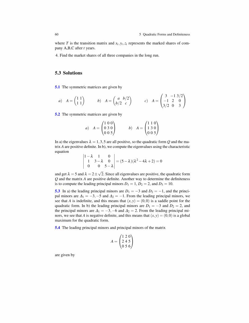
60 5 Quadratic Forms and Definiteness
where T is the transition matrix and xt ,yt ,zt represents the marked shares of com-pany A,B,C after t years.
4. Find the market shares of all three companies in the long run.
5.3 Solutions
5.1 The symmetric matrices are given by
a) A =
(1 11 1
)b) A =
(a b/2
b/2 c
)c) A =
3 −1 3/2−1 2 03/2 0 3
5.2 The symmetric matrices are given by
a) A =
1 0 00 3 00 0 5
b) A =
1 1 01 3 00 0 5
In a) the eigenvalues λ = 1,3,5 are all positive, so the quadratic form Q and the ma-trix A are positive definite. In b), we compute the eigenvalues using the characteristicequation ∣∣∣∣∣∣
1−λ 1 01 3−λ 00 0 5−λ
∣∣∣∣∣∣= (5−λ )(λ 2−4λ +2) = 0
and get λ = 5 and λ = 2±√
2. Since all eigenvalues are positive, the quadratic formQ and the matrix A are positive definite. Another way to determine the definitenessis to compute the leading principal minors D1 = 1, D2 = 2, and D3 = 10.
5.3 In a) the leading principal minors are D1 = −3 and D2 = −1, and the princi-pal minors are ∆1 = −3,−5 and ∆2 = −1. From the leading principal minors, wesee that A is indefinite, and this means that (x,y) = (0,0) is a saddle point for thequadratic form. In b) the leading principal minors are D1 = −3 and D2 = 2, andthe principal minors are ∆1 = −3,−6 and ∆2 = 2. From the leading principal mi-nors, we see that A is negative definite, and this means that (x,y) = (0,0) is a globalmaximum for the quadratic form.
5.4 The leading principal minors and principal minors of the matrix
A =
1 2 02 4 50 5 6
are given by
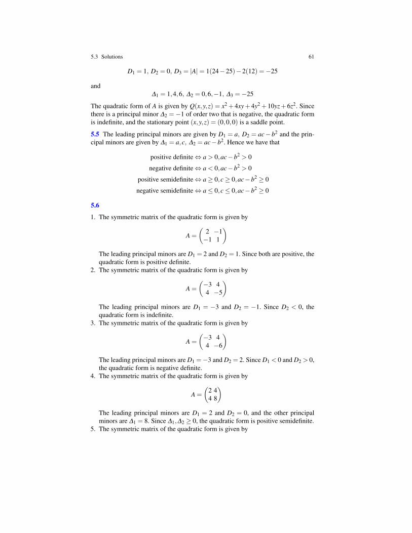
5.3 Solutions 61
D1 = 1, D2 = 0, D3 = |A|= 1(24−25)−2(12) =−25
and∆1 = 1,4,6, ∆2 = 0,6,−1, ∆3 =−25
The quadratic form of A is given by Q(x,y,z) = x2 +4xy+4y2 +10yz+6z2. Sincethere is a principal minor ∆2 =−1 of order two that is negative, the quadratic formis indefinite, and the stationary point (x,y,z) = (0,0,0) is a saddle point.
5.5 The leading principal minors are given by D1 = a, D2 = ac−b2 and the prin-cipal minors are given by ∆1 = a,c, ∆2 = ac−b2. Hence we have that
positive definite⇔ a > 0,ac−b2 > 0
negative definite⇔ a < 0,ac−b2 > 0
positive semidefinite⇔ a≥ 0,c≥ 0,ac−b2 ≥ 0
negative semidefinite⇔ a≤ 0,c≤ 0,ac−b2 ≥ 0
5.6
1. The symmetric matrix of the quadratic form is given by
A =
(2 −1−1 1
)The leading principal minors are D1 = 2 and D2 = 1. Since both are positive, thequadratic form is positive definite.
2. The symmetric matrix of the quadratic form is given by
A =
(−3 44 −5
)The leading principal minors are D1 = −3 and D2 = −1. Since D2 < 0, thequadratic form is indefinite.
3. The symmetric matrix of the quadratic form is given by
A =
(−3 44 −6
)The leading principal minors are D1 =−3 and D2 = 2. Since D1 < 0 and D2 > 0,the quadratic form is negative definite.
4. The symmetric matrix of the quadratic form is given by
A =
(2 44 8
)The leading principal minors are D1 = 2 and D2 = 0, and the other principalminors are ∆1 = 8. Since ∆1,∆2 ≥ 0, the quadratic form is positive semidefinite.
5. The symmetric matrix of the quadratic form is given by
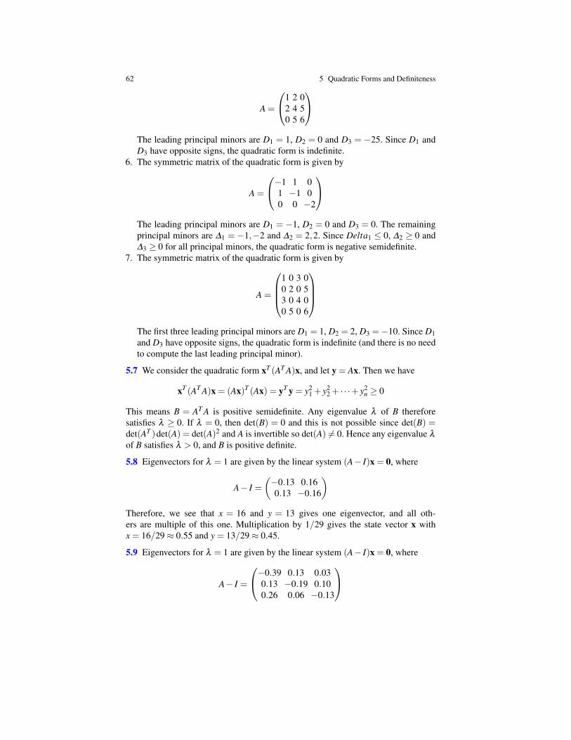
62 5 Quadratic Forms and Definiteness
A =
1 2 02 4 50 5 6
The leading principal minors are D1 = 1, D2 = 0 and D3 = −25. Since D1 andD3 have opposite signs, the quadratic form is indefinite.
6. The symmetric matrix of the quadratic form is given by
A =
−1 1 01 −1 00 0 −2
The leading principal minors are D1 = −1, D2 = 0 and D3 = 0. The remainingprincipal minors are ∆1 = −1,−2 and ∆2 = 2,2. Since Delta1 ≤ 0, ∆2 ≥ 0 and∆3 ≥ 0 for all principal minors, the quadratic form is negative semidefinite.
7. The symmetric matrix of the quadratic form is given by
A =
1 0 3 00 2 0 53 0 4 00 5 0 6
The first three leading principal minors are D1 = 1, D2 = 2, D3 =−10. Since D1and D3 have opposite signs, the quadratic form is indefinite (and there is no needto compute the last leading principal minor).
5.7 We consider the quadratic form xT (AT A)x, and let y = Ax. Then we have
xT (AT A)x = (Ax)T (Ax) = yT y = y21 + y2
2 + · · ·+ y2n ≥ 0
This means B = AT A is positive semidefinite. Any eigenvalue λ of B thereforesatisfies λ ≥ 0. If λ = 0, then det(B) = 0 and this is not possible since det(B) =det(AT )det(A) = det(A)2 and A is invertible so det(A) 6= 0. Hence any eigenvalue λ
of B satisfies λ > 0, and B is positive definite.
5.8 Eigenvectors for λ = 1 are given by the linear system (A− I)x = 0, where
A− I =(−0.13 0.160.13 −0.16
)Therefore, we see that x = 16 and y = 13 gives one eigenvector, and all oth-ers are multiple of this one. Multiplication by 1/29 gives the state vector x withx = 16/29≈ 0.55 and y = 13/29≈ 0.45.
5.9 Eigenvectors for λ = 1 are given by the linear system (A− I)x = 0, where
A− I =
−0.39 0.13 0.030.13 −0.19 0.100.26 0.06 −0.13
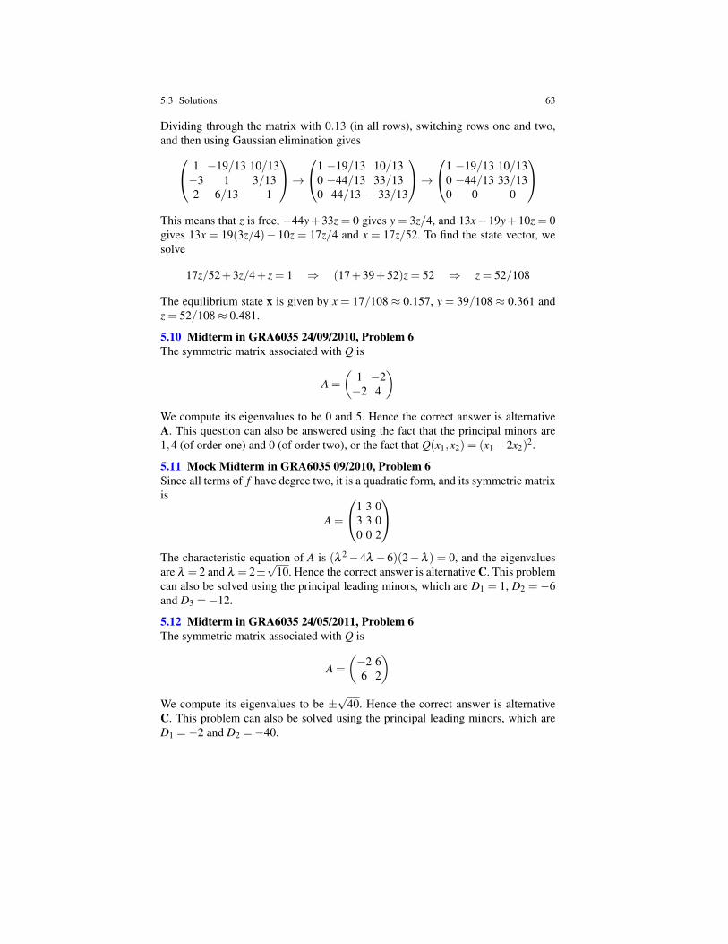
5.3 Solutions 63
Dividing through the matrix with 0.13 (in all rows), switching rows one and two,and then using Gaussian elimination gives 1 −19/13 10/13
−3 1 3/132 6/13 −1
→1 −19/13 10/13
0 −44/13 33/130 44/13 −33/13
→1 −19/13 10/13
0 −44/13 33/130 0 0
This means that z is free, −44y+33z = 0 gives y = 3z/4, and 13x−19y+10z = 0gives 13x = 19(3z/4)− 10z = 17z/4 and x = 17z/52. To find the state vector, wesolve
17z/52+3z/4+ z = 1 ⇒ (17+39+52)z = 52 ⇒ z = 52/108
The equilibrium state x is given by x = 17/108 ≈ 0.157, y = 39/108 ≈ 0.361 andz = 52/108≈ 0.481.
5.10 Midterm in GRA6035 24/09/2010, Problem 6The symmetric matrix associated with Q is
A =
(1 −2−2 4
)We compute its eigenvalues to be 0 and 5. Hence the correct answer is alternativeA. This question can also be answered using the fact that the principal minors are1,4 (of order one) and 0 (of order two), or the fact that Q(x1,x2) = (x1−2x2)
2.
5.11 Mock Midterm in GRA6035 09/2010, Problem 6Since all terms of f have degree two, it is a quadratic form, and its symmetric matrixis
A =
1 3 03 3 00 0 2
The characteristic equation of A is (λ 2− 4λ − 6)(2−λ ) = 0, and the eigenvaluesare λ = 2 and λ = 2±
√10. Hence the correct answer is alternative C. This problem
can also be solved using the principal leading minors, which are D1 = 1, D2 = −6and D3 =−12.
5.12 Midterm in GRA6035 24/05/2011, Problem 6The symmetric matrix associated with Q is
A =
(−2 66 2
)We compute its eigenvalues to be ±
√40. Hence the correct answer is alternative
C. This problem can also be solved using the principal leading minors, which areD1 =−2 and D2 =−40.
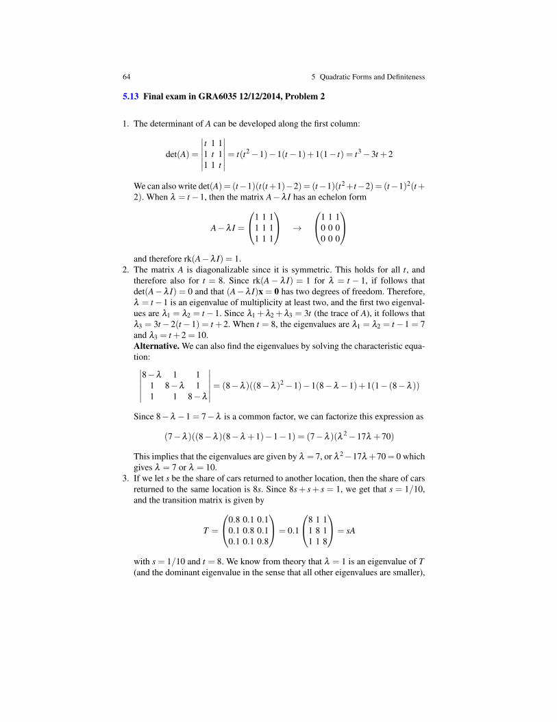
64 5 Quadratic Forms and Definiteness
5.13 Final exam in GRA6035 12/12/2014, Problem 2
1. The determinant of A can be developed along the first column:
det(A) =
∣∣∣∣∣∣t 1 11 t 11 1 t
∣∣∣∣∣∣= t(t2−1)−1(t−1)+1(1− t) = t3−3t +2
We can also write det(A)= (t−1)(t(t+1)−2)= (t−1)(t2+t−2)= (t−1)2(t+2). When λ = t−1, then the matrix A−λ I has an echelon form
A−λ I =
1 1 11 1 11 1 1
→
1 1 10 0 00 0 0
and therefore rk(A−λ I) = 1.
2. The matrix A is diagonalizable since it is symmetric. This holds for all t, andtherefore also for t = 8. Since rk(A− λ I) = 1 for λ = t − 1, if follows thatdet(A−λ I) = 0 and that (A−λ I)x = 0 has two degrees of freedom. Therefore,λ = t−1 is an eigenvalue of multiplicity at least two, and the first two eigenval-ues are λ1 = λ2 = t−1. Since λ1 +λ2 +λ3 = 3t (the trace of A), it follows thatλ3 = 3t−2(t−1) = t +2. When t = 8, the eigenvalues are λ1 = λ2 = t−1 = 7and λ3 = t +2 = 10.Alternative. We can also find the eigenvalues by solving the characteristic equa-tion:∣∣∣∣∣∣
8−λ 1 11 8−λ 11 1 8−λ
∣∣∣∣∣∣= (8−λ )((8−λ )2−1)−1(8−λ −1)+1(1− (8−λ ))
Since 8−λ −1 = 7−λ is a common factor, we can factorize this expression as
(7−λ )((8−λ )(8−λ +1)−1−1) = (7−λ )(λ 2−17λ +70)
This implies that the eigenvalues are given by λ = 7, or λ 2−17λ +70 = 0 whichgives λ = 7 or λ = 10.
3. If we let s be the share of cars returned to another location, then the share of carsreturned to the same location is 8s. Since 8s+ s+ s = 1, we get that s = 1/10,and the transition matrix is given by
T =
0.8 0.1 0.10.1 0.8 0.10.1 0.1 0.8
= 0.1
8 1 11 8 11 1 8
= sA
with s = 1/10 and t = 8. We know from theory that λ = 1 is an eigenvalue of T(and the dominant eigenvalue in the sense that all other eigenvalues are smaller),
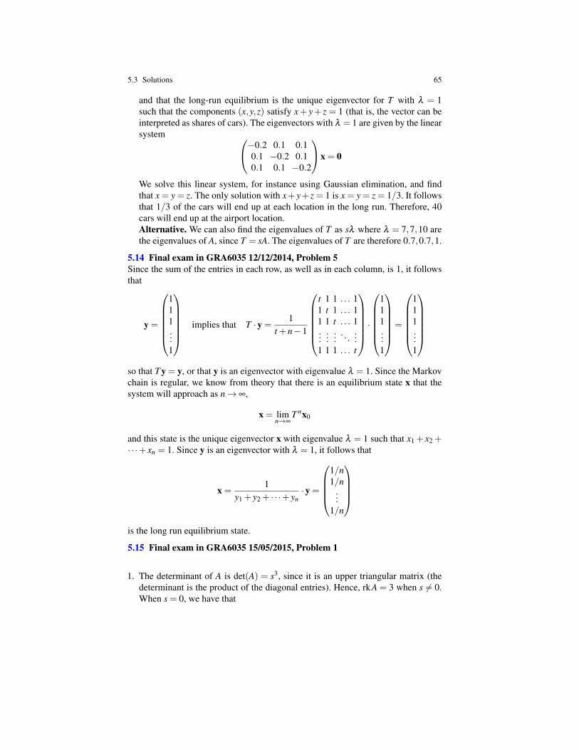
5.3 Solutions 65
and that the long-run equilibrium is the unique eigenvector for T with λ = 1such that the components (x,y,z) satisfy x+ y+ z = 1 (that is, the vector can beinterpreted as shares of cars). The eigenvectors with λ = 1 are given by the linearsystem −0.2 0.1 0.1
0.1 −0.2 0.10.1 0.1 −0.2
x = 0
We solve this linear system, for instance using Gaussian elimination, and findthat x = y = z. The only solution with x+y+ z = 1 is x = y = z = 1/3. It followsthat 1/3 of the cars will end up at each location in the long run. Therefore, 40cars will end up at the airport location.Alternative. We can also find the eigenvalues of T as sλ where λ = 7,7,10 arethe eigenvalues of A, since T = sA. The eigenvalues of T are therefore 0.7,0.7,1.
5.14 Final exam in GRA6035 12/12/2014, Problem 5Since the sum of the entries in each row, as well as in each column, is 1, it followsthat
y =
111...1
implies that T ·y =1
t +n−1
t 1 1 . . . 11 t 1 . . . 11 1 t . . . 1...
......
. . ....
1 1 1 . . . t
·
111...1
=
111...1
so that T y = y, or that y is an eigenvector with eigenvalue λ = 1. Since the Markovchain is regular, we know from theory that there is an equilibrium state x that thesystem will approach as n→ ∞,
x = limn→∞
T nx0
and this state is the unique eigenvector x with eigenvalue λ = 1 such that x1 + x2 +· · ·+ xn = 1. Since y is an eigenvector with λ = 1, it follows that
x =1
y1 + y2 + · · ·+ yn·y =
1/n1/n
...1/n
is the long run equilibrium state.
5.15 Final exam in GRA6035 15/05/2015, Problem 1
1. The determinant of A is det(A) = s3, since it is an upper triangular matrix (thedeterminant is the product of the diagonal entries). Hence, rkA = 3 when s 6= 0.When s = 0, we have that
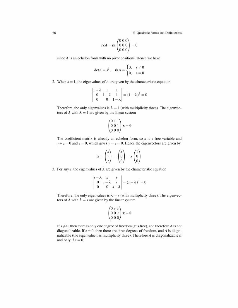
66 5 Quadratic Forms and Definiteness
rkA = rk
0 0 00 0 00 0 0
= 0
since A is an echelon form with no pivot positions. Hence we have
detA = s3, rkA =
{3, s 6= 00, s = 0
2. When s = 1, the eigenvalues of A are given by the characteristic equation∣∣∣∣∣∣1−λ 1 1
0 1−λ 10 0 1−λ
∣∣∣∣∣∣= (1−λ )3 = 0
Therefore, the only eigenvalues is λ = 1 (with multiplicity three). The eigenvec-tors of A with λ = 1 are given by the linear system0 1 1
0 0 10 0 0
x = 0
The coefficient matrix is already an echelon form, so x is a free variable andy+ z = 0 and z = 0, which gives y = z = 0. Hence the eigenvectors are given by
x =
xyz
=
x00
= x
100
3. For any s, the eigenvalues of A are given by the characteristic equation∣∣∣∣∣∣
s−λ s s0 s−λ s0 0 s−λ
∣∣∣∣∣∣= (s−λ )3 = 0
Therefore, the only eigenvalues is λ = s (with multiplicity three). The eigenvec-tors of A with λ = s are given by the linear system0 s s
0 0 s0 0 0
x = 0
If s 6= 0, then there is only one degree of freedom (x is free), and therefore A is notdiagonalizable. If s = 0, then there are three degrees of freedom, and A is diago-nalizable (the eigenvalue has multiplicity three). Therefore A is diagonalizable ifand only if s = 0.
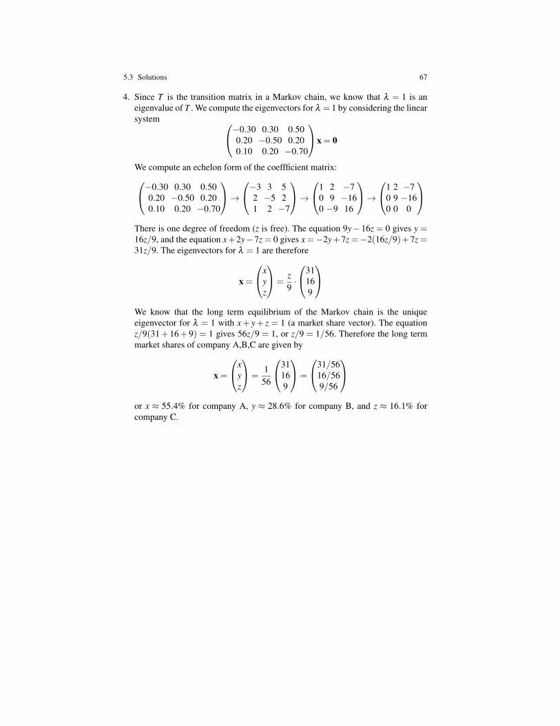
5.3 Solutions 67
4. Since T is the transition matrix in a Markov chain, we know that λ = 1 is aneigenvalue of T . We compute the eigenvectors for λ = 1 by considering the linearsystem −0.30 0.30 0.50
0.20 −0.50 0.200.10 0.20 −0.70
x = 0
We compute an echelon form of the coeffficient matrix:−0.30 0.30 0.500.20 −0.50 0.200.10 0.20 −0.70
→−3 3 5
2 −5 21 2 −7
→1 2 −7
0 9 −160 −9 16
→1 2 −7
0 9 −160 0 0
There is one degree of freedom (z is free). The equation 9y−16z = 0 gives y =16z/9, and the equation x+2y−7z = 0 gives x =−2y+7z =−2(16z/9)+7z =31z/9. The eigenvectors for λ = 1 are therefore
x =
xyz
=z9·
31169
We know that the long term equilibrium of the Markov chain is the uniqueeigenvector for λ = 1 with x+ y+ z = 1 (a market share vector). The equationz/9(31+ 16+ 9) = 1 gives 56z/9 = 1, or z/9 = 1/56. Therefore the long termmarket shares of company A,B,C are given by
x =
xyz
=156
31169
=
31/5616/569/56
or x ≈ 55.4% for company A, y ≈ 28.6% for company B, and z ≈ 16.1% forcompany C.

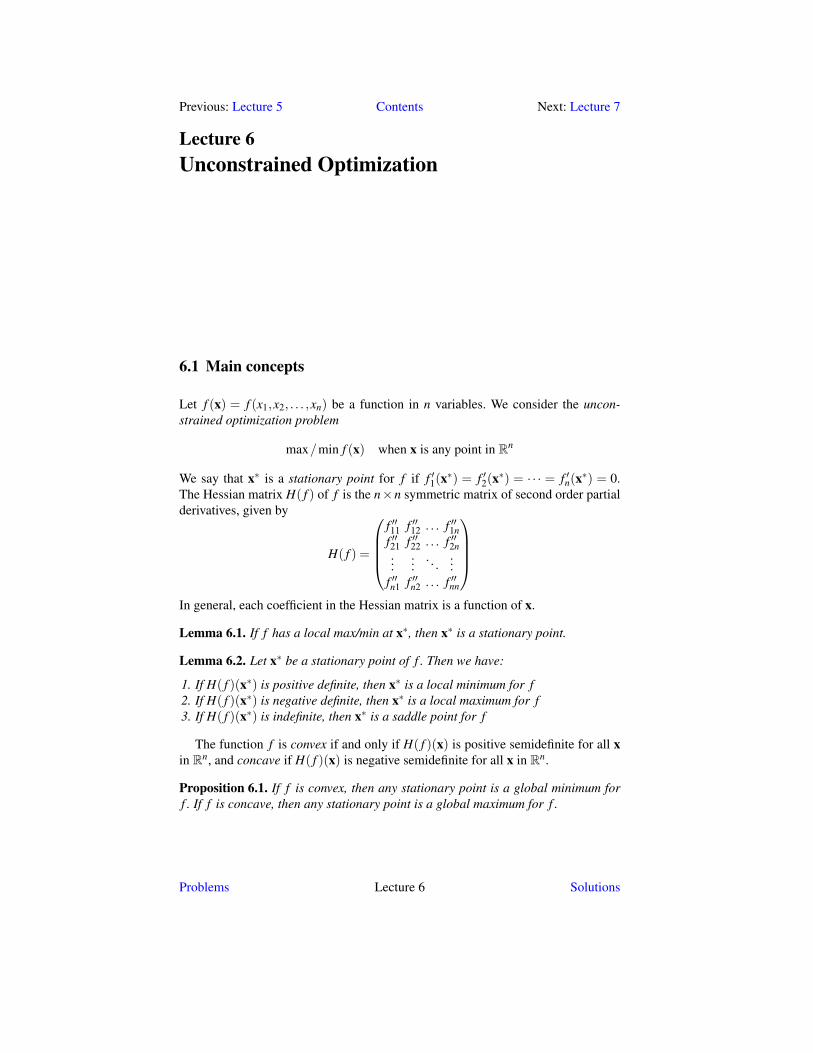
Previous: Lecture 5 Contents Next: Lecture 7
Lecture 6Unconstrained Optimization
6.1 Main concepts
Let f (x) = f (x1,x2, . . . ,xn) be a function in n variables. We consider the uncon-strained optimization problem
max/min f (x) when x is any point in Rn
We say that x∗ is a stationary point for f if f ′1(x∗) = f ′2(x
∗) = · · · = f ′n(x∗) = 0.The Hessian matrix H( f ) of f is the n×n symmetric matrix of second order partialderivatives, given by
H( f ) =
f ′′11 f ′′12 . . . f ′′1nf ′′21 f ′′22 . . . f ′′2n...
.... . .
...f ′′n1 f ′′n2 . . . f ′′nn
In general, each coefficient in the Hessian matrix is a function of x.
Lemma 6.1. If f has a local max/min at x∗, then x∗ is a stationary point.
Lemma 6.2. Let x∗ be a stationary point of f . Then we have:
1. If H( f )(x∗) is positive definite, then x∗ is a local minimum for f2. If H( f )(x∗) is negative definite, then x∗ is a local maximum for f3. If H( f )(x∗) is indefinite, then x∗ is a saddle point for f
The function f is convex if and only if H( f )(x) is positive semidefinite for all xin Rn, and concave if H( f )(x) is negative semidefinite for all x in Rn.
Proposition 6.1. If f is convex, then any stationary point is a global minimum forf . If f is concave, then any stationary point is a global maximum for f .
Problems Lecture 6 Solutions
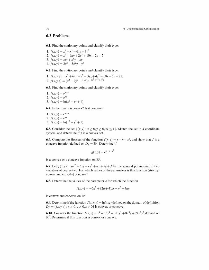
70 6 Unconstrained Optimization
6.2 Problems
6.1. Find the stationary points and classify their type:
1. f (x,y) = x4 + x2−6xy+3y2
2. f (x,y) = x2−6xy+2y2 +10x+2y−53. f (x,y) = xy2 + x3y− xy4. f (x,y) = 3x4 +3x2y− y3
6.2. Find the stationary points and classify their type:
1. f (x,y,z) = x2 +6xy+ y2−3yz+4z2−10x−5y−21z2. f (x,y,z) = (x2 +2y2 +3z2)e−(x
2+y2+z2)
6.3. Find the stationary points and classify their type:
1. f (x,y) = ex+y
2. f (x,y) = exy
3. f (x,y) = ln(x2 + y2 +1)
6.4. Is the function convex? Is it concave?
1. f (x,y) = ex+y
2. f (x,y) = exy
3. f (x,y) = ln(x2 + y2 +1)
6.5. Consider the set {(x,y) : x ≥ 0,y ≥ 0,xy ≤ 1}. Sketch the set in a coordinatesystem, and determine if it is a convex set.
6.6. Compute the Hessian of the function f (x,y) = x− y− x2, and show that f is aconcave function defined on D f = R2. Determine if
g(x,y) = ex−y−x2
is a convex or a concave function on R2.
6.7. Let f (x,y) = ax2 + bxy+ cy2 + dx+ ey+ f be the general polynomial in twovariables of degree two. For which values of the parameters is this function (strictly)convex and (strictly) concave?
6.8. Determine the values of the parameter a for which the function
f (x,y) =−6x2 +(2a+4)xy− y2 +4ay
is convex and concave on R2.
6.9. Determine if the function f (x,y,z)= ln(xyz) defined on the domain of definitionD f = {(x,y,z) : x > 0,y > 0,z > 0} is convex or concave.
6.10. Consider the function f (x,y) = x4 +16y4 +32xy3 +8x3y+24x2y2 defined onR2. Determine if this function is convex or concave.
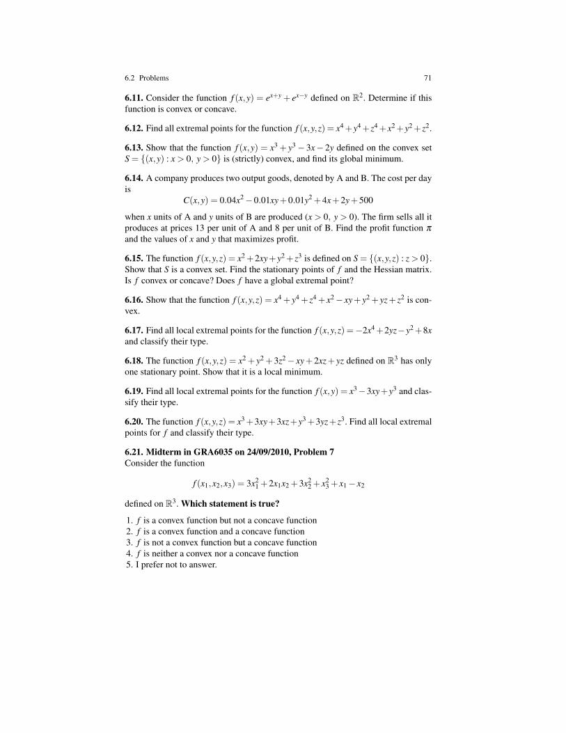
6.2 Problems 71
6.11. Consider the function f (x,y) = ex+y + ex−y defined on R2. Determine if thisfunction is convex or concave.
6.12. Find all extremal points for the function f (x,y,z) = x4+y4+z4+x2+y2+z2.
6.13. Show that the function f (x,y) = x3 + y3− 3x− 2y defined on the convex setS = {(x,y) : x > 0, y > 0} is (strictly) convex, and find its global minimum.
6.14. A company produces two output goods, denoted by A and B. The cost per dayis
C(x,y) = 0.04x2−0.01xy+0.01y2 +4x+2y+500
when x units of A and y units of B are produced (x > 0, y > 0). The firm sells all itproduces at prices 13 per unit of A and 8 per unit of B. Find the profit function π
and the values of x and y that maximizes profit.
6.15. The function f (x,y,z) = x2 +2xy+y2 + z3 is defined on S = {(x,y,z) : z > 0}.Show that S is a convex set. Find the stationary points of f and the Hessian matrix.Is f convex or concave? Does f have a global extremal point?
6.16. Show that the function f (x,y,z) = x4 + y4 + z4 + x2− xy+ y2 + yz+ z2 is con-vex.
6.17. Find all local extremal points for the function f (x,y,z) =−2x4+2yz−y2+8xand classify their type.
6.18. The function f (x,y,z) = x2 + y2 +3z2− xy+2xz+ yz defined on R3 has onlyone stationary point. Show that it is a local minimum.
6.19. Find all local extremal points for the function f (x,y) = x3−3xy+y3 and clas-sify their type.
6.20. The function f (x,y,z) = x3+3xy+3xz+y3+3yz+ z3. Find all local extremalpoints for f and classify their type.
6.21. Midterm in GRA6035 on 24/09/2010, Problem 7Consider the function
f (x1,x2,x3) = 3x21 +2x1x2 +3x2
2 + x23 + x1− x2
defined on R3. Which statement is true?
1. f is a convex function but not a concave function2. f is a convex function and a concave function3. f is not a convex function but a concave function4. f is neither a convex nor a concave function5. I prefer not to answer.
72 6 Unconstrained Optimization
6.22. Mock Midterm in GRA6035 on 09/2010, Problem 7Consider the function
f (x1,x2) = 3−a ·Q(x1,x2)
defined on R2, where a ∈ R is a number and Q is a positive definite quadratic form.Which statement is true?
1. f is convex for all values of a2. f is concave for all values of a3. f is convex if a≥ 0 and concave if a≤ 04. f is convex if a≤ 0 and concave if a≥ 05. I prefer not to answer.
6.23. Midterm in GRA6035 on 24/05/2011, Problem 7Consider the function
f (x1,x2,x3) =−x21 +2x1x2−3x2
2− x23− x1− x3
defined on R3. Which statement is true?
1. f is a convex function but not a concave function2. f is a convex function and a concave function3. f is not a convex function but a concave function4. f is neither a convex nor a concave function5. I prefer not to answer.
6.24. Final Exam in GRA6035 on 10/12/2010, Problem 1We consider the function f (x,y,z) = x2ex + yz− z3.
1. Find all stationary points of f .2. Compute the Hessian matrix of f . Classify the stationary points of f as local
maxima, local minima or saddle points.
6.25. Mock Final Exam in GRA6035 on 12/2010, Problem 2
1. Find all stationary points of f (x,y,z) = exy+yz−xz.2. The function g(x,y,z) = eax+by+cz is defined on R3. Determine the values of the
parameters a,b,c such that g is convex. Is it concave for any values of a,b,c?
6.26. Final Exam in GRA6035 on 30/05/2011, Problem 1We consider the function f (x,y,z,w) = x5 + xy2− zw.
1. Find all stationary points of f .2. Compute the Hessian matrix of f . Classify the stationary points of f as local
maxima, local minima or saddle points.
6.3 Solutions 73
6.3 Solutions
6.1 In each case, we compute the first order partial derivatives and solve the firstorder conditions to find the stationary points. Then we compute the Hessian anddetermine the definiteness of the Hessian at each stationary point to classify it.
1. The first order conditions (FOC) are given by
f ′x = 4x3 +2x−6y = 0, f ′y =−6x+6y = 0
From the second equation x= y, and the first then gives 4x3−4x= 4x(x2−1)= 0,or x = 0 or x = ±1. The stationary points are (0,0), (1,1) and (−1,−1). TheHessian matrix is given by
H( f ) =(
12x2 +2 −6−6 6
)At (0,0) we have D1 = 2 and D2 = 12−36 = −24. This point is a saddle pointsince D2 is negative. At (±1,±1) we have D1 = 14 and D2 = 84− 36 = 48.These points are local minima since D1,D2 > 0.
2. The first order conditions (FOC) are given by
f ′x = 2x−6y+10 = 0, f ′y =−6x+4y+2 = 0
We combine the equations to get −14y+32 = 0 or y = 32/14 = 16/7, and thenx = 3(16/7)−5 = 13/7. The unique stationary point is (13/7,16/7). The Hes-sian matrix is given by
H( f ) =(
2 −6−6 4
)and D1 = 2, D2 = 8−36 =−28. The stationary point is a saddle point since D2is negative.
3. The first order conditions (FOC) are given by
f ′x = y2+3x2y−y = y(y+3x2−1) = 0, f ′y = 2xy+x3−x = x(2y+x2−1) = 0
From the second equation either x = 0 or x2 = 1−2y. In the first equation, x = 0gives y2− y = 0, that is y = 0 or y = 1, and the stationary points in this case are(0,0) and (0,1). The other possibility is x 6= 0 but x2 = 1−2y. In this case, the firstequation gives y = 0 or y+3x2−1 = 0. If y = 0 then x =±1, and if y = 1−3x2,then x2 = 1−2(1−3x2) = 6x2−1, or x = ±1/
√5. This gives stationary points
(±1,0) and (±1/√
5,2/5). The Hessian matrix is given by
H( f ) =(
6xy 2y+3x2−12y+3x2−1 2x
)
74 6 Unconstrained Optimization
At (0,0) and (0,1), we have D1 = 0 and D2 = −1. These points are saddlepoints since D2 is negative. At (±1,0) we have D1 = 0 and D2 = −4. Thesepoints are also saddle points since D2 is negative. At (±1/
√5,2/5), we have
D1 = 12x/5 and D2 = 12(1/5)(2/5)−(4/5+3/5−1)2 = 20/25. This is positivedefinite when x is positive, and negative definite when x is negative. Therefore(1/√
5,2/5) is a local minimum and (−1/√
5,2/5) is a local maximum4. The first order conditions (FOC) are given by
f ′x = 12x3 +6xy = 0, f ′y = 3x2−3y2 = 0
From the second equation x2 = y2, and therefore x = y or x = −y. If x = y, thefirst equation gives 12x3+6x2 = 6x2(2x+1) = 0, that is x = 0 or x =−1/2. Thisgives stationary points (0,0) and (−1/2,−1/2). If x =−y then the first equationgives 12x3− 6x2 = 6x2(2x− 1), that is x = 0 or x = 1/2. This gives stationarypoints (0,0 (again) and (1/2,−1/2). The Hessian matrix is given by
H( f ) =(
36x2 +6y 6x6x −6y
)At (±1/2,−1/2) we have D1 = 6 and D2 = 18− 9 = 9. These points are localminima since D1,D2 are positive. At (0,0) the Hessian matrix is the zero matrix,and the second derivative test is inconclusive. Along the path where x = 0 andy = a (the y-axis), we have that f (0,a) =−a3. Since f (0,a) is negative for a > 0and positiv for a < 0, the stationary point (0,0) at a = 0 is a saddle point.
6.2
1. The first order conditions (FOC) are given by
f ′x = 2x+6y−10 = 0, f ′y = 6x+2y−3z−5 = 0, f ′z =−3y+8z−21 = 0
The unique stationary point is (x,y,z) = (2,1,3), and we find it by solving thelinear system (for instance using Gaussian elimination). The Hessian is indefiniteat this stationary point since the Hessian matrix
H( f ) =
2 6 06 2 −30 −3 8
has leading principal minors D1 = 2 and D2 =−32 (there is no need to computethe last leading principal minor). The stationary point (2,1,3) is a saddle pointfor f .
2. Let us write u= x2+2y2+3z2 and v=−(x2+y2+z2). The first order conditions(FOC) are given by
6.3 Solutions 75
f ′x = 2xev +uev(−2x) = 2xev(1−u)
f ′y = 4yev +uev(−2y) = 2yev(2−u)
f ′z = 6zev +uev(−2z) = 2zev(3−u)
If u = 1, then y = z = 0, and x = ±1. If u = 2, then x = z = 0 and y = ±1. Ifu = 3, then x = y = 0 and z = ±1. If u 6= 1,2,3 then x = y = z = 0. We find thestationary points (±1,0,0), (0,±1,0), (0,0,±1) and (0,0,0). To compute theHessian matrix, notice that
f ′′xx = (2(1−u)+2x(−2x))ev +2x(1−u)ev(−2x) = 2ev(1−u−2x2(2−u))
The other second order principal minors can be computed similarly. We find thatthe Hessian matrix is given by
H( f ) = 2ev
(1−u)−2x2(2−u) −2xy(3−u) −2xz(4−u)−2xy(3−u) (2−u)−2y2(4−u) −2yz(5−u)−2xz(4−u) −2yz(5−u) (3−u)−2z2(6−u)
At all stationary points, xy = xz = yz = 0 so that the Hessian matrix is diago-nal. At (0,0,0), the diagonal entries are (2,4,6) and are all positive. The point(0,0,0) is therefore a local minimum point. At (±1,0,0), the diagonal entriesare 2e−1(−2,1,2), and at (0,±1,0) the diagonal entries are 2e−1(−1,−4,1). Inboth cases, the diagonal contains both positive and negative entries, and thesestationary points are therefore saddle points. At (0,0,±1), the diagonal entriesare 2e−1(−2,−1,−6) and are all negative. The points (0,0,±1) are thereforelocal maxima.
6.3
1. The function f (x,y) = ex+y has partial derivatives f ′1 = f ′2 = ex+y, hence thereare no stationary points.
2. The function f (x,y) = exy has partial derivatives f ′1 = yexy and f ′2 = xexy. Hencethe stationary points are given by yexy = xexy = 0, and we see that there is aunique stationary point (x,y) = (0,0). The Hessian matrix is
H( f )(0,0) =(
y2exy (1+ xy)exy
(1+ xy)exy x2exy
)(0,0) =
(0 11 0
)This matrix is indefinite since D2 =−1, and (0,0) is a saddle point.
3. The function f (x,y)= ln(x2+y2+1) has partial derivatives f ′1 = 2x/(x2+y2+1)and f ′2 = 2y/(x2+y2+1). Hence there is a unique stationary point (x,y) = (0,0).The Hessian matrix is
H( f )(0,0) =
−2x2+2y2+2(x2+y2+1)2
−4xy(x2+y2+1)2
−4xy(x2+y2+1)2
2x2−2y2+2(x2+y2+1)2
(0,0) =(
2 00 2
)
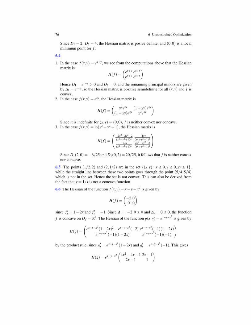
76 6 Unconstrained Optimization
Since D1 = 2, D2 = 4, the Hessian matrix is posive definte, and (0,0) is a localminimum point for f .
6.4
1. In the case f (x,y) = ex+y, we see from the computations above that the Hessianmatrix is
H( f ) =(
ex+y ex+y
ex+y ex+y
)Hence D1 = ex+y > 0 and D2 = 0, and the remaining principal minors are givenby ∆1 = ex+y, so the Hessian matrix is positive semidefinite for all (x,y) and f isconvex.
2. In the case f (x,y) = exy, the Hessian matrix is
H( f ) =(
y2exy (1+ xy)exy
(1+ xy)exy x2exy
)Since it is indefinite for (x,y) = (0,0), f is neither convex nor concave.
3. In the case f (x,y) = ln(x2 + y2 +1), the Hessian matrix is
H( f ) =
−2x2+2y2+2(x2+y2+1)2
−4xy(x2+y2+1)2
−4xy(x2+y2+1)2
2x2−2y2+2(x2+y2+1)2
Since D1(2,0) =−6/25 and D1(0,2) = 20/25, it follows that f is neither convexnor concave.
6.5 The points (1/2,2) and (2,1/2) are in the set {(x,y) : x ≥ 0,y ≥ 0,xy ≤ 1},while the straight line between these two points goes through the point (5/4,5/4)which is not in the set. Hence the set is not convex. This can also be derived fromthe fact that y = 1/x is not a concave function.
6.6 The Hessian of the function f (x,y) = x− y− x2 is given by
H( f ) =(−2 00 0
)since f ′x = 1−2x and f ′y =−1. Since ∆1 =−2,0≤ 0 and ∆2 = 0≥ 0, the function
f is concave on D f = R2. The Hessian of the function g(x,y) = ex−y−x2is given by
H(g) =
(ex−y−x2
(1−2x)2 + ex−y−x2(−2) ex−y−x2
(−1)(1−2x)ex−y−x2
(−1)(1−2x) ex−y−x2(−1)(−1)
)
by the product rule, since g′x = ex−y−x2(1−2x) and g′y = ex−y−x2
(−1). This gives
H(g) = ex−y−x2(
4x2−4x−1 2x−12x−1 1
)
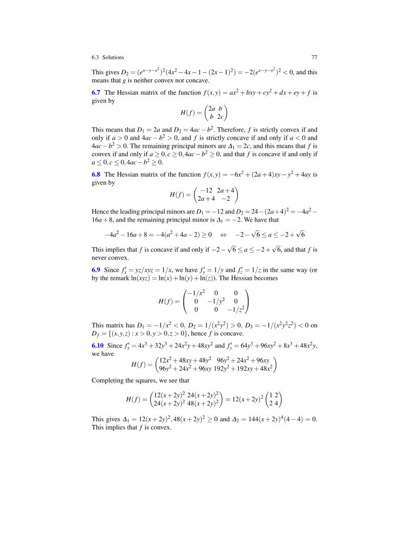
6.3 Solutions 77
This gives D2 = (ex−y−x2)2(4x2−4x−1− (2x−1)2) =−2(ex−y−x2
)2 < 0, and thismeans that g is neither convex nor concave.
6.7 The Hessian matrix of the function f (x,y) = ax2 + bxy+ cy2 + dx+ ey+ f isgiven by
H( f ) =(
2a bb 2c
)This means that D1 = 2a and D2 = 4ac− b2. Therefore, f is strictly convex if andonly if a > 0 and 4ac− b2 > 0, and f is strictly concave if and only if a < 0 and4ac−b2 > 0. The remaining principal minors are ∆1 = 2c, and this means that f isconvex if and only if a≥ 0,c≥ 0,4ac−b2 ≥ 0, and that f is concave if and only ifa≤ 0,c≤ 0,4ac−b2 ≥ 0.
6.8 The Hessian matrix of the function f (x,y) = −6x2 +(2a+ 4)xy− y2 + 4ay isgiven by
H( f ) =(−12 2a+4
2a+4 −2
)Hence the leading principal minors are D1 =−12 and D2 = 24−(2a+4)2 =−4a2−16a+8, and the remaining principal minor is ∆1 =−2. We have that
−4a2−16a+8 =−4(a2 +4a−2)≥ 0 ⇔ −2−√
6≤ a≤−2+√
6
This implies that f is concave if and only if −2−√
6≤ a≤−2+√
6, and that f isnever convex.
6.9 Since f ′x = yz/xyz = 1/x, we have f ′y = 1/y and f ′z = 1/z in the same way (orby the remark ln(xyz) = ln(x)+ ln(y)+ ln(z)). The Hessian becomes
H( f ) =
−1/x2 0 00 −1/y2 00 0 −1/z2
This matrix has D1 = −1/x2 < 0, D2 = 1/(x2y2) > 0, D3 = −1/(x2y2z2) < 0 onD f = {(x,y,z) : x > 0,y > 0,z > 0}, hence f is concave.
6.10 Since f ′x = 4x3 +32y3 +24x2y+48xy2 and f ′y = 64y3 +96xy2 +8x3 +48x2y,we have
H( f ) =(
12x2 +48xy+48y2 96y2 +24x2 +96xy96y2 +24x2 +96xy 192y2 +192xy+48x2
)Completing the squares, we see that
H( f ) =(
12(x+2y)2 24(x+2y)2
24(x+2y)2 48(x+2y)2
)= 12(x+2y)2
(1 22 4
)This gives ∆1 = 12(x+ 2y)2,48(x+ 2y)2 ≥ 0 and ∆2 = 144(x+ 2y)4(4− 4) = 0.This implies that f is convex.
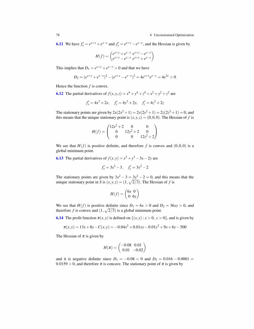
78 6 Unconstrained Optimization
6.11 We have f ′x = ex+y + ex−y and f ′y = ex+y− ex−y, and the Hessian is given by
H( f ) =(
ex+y + ex−y ex+y− ex−y
ex+y− ex−y ex+y + ex−y
)This implies that D1 = ex+y + ex−y > 0 and that we have
D2 = (ex+y + ex−y)2− (ex+y− ex−y)2 = 4ex+yex−y = 4e2x > 0
Hence the function f is convex.
6.12 The partial derivatives of f (x,y,z) = x4 + y4 + z4 + x2 + y2 + z2 are
f ′x = 4x3 +2x, f ′y = 4y3 +2y, f ′z = 4z3 +2z
The stationary points are given by 2x(2x2+1) = 2y(2y2+1) = 2z(2z2+1) = 0, andthis means that the unique stationary point is (x,y,z) = (0,0,0). The Hessian of f is
H( f ) =
12x2 +2 0 00 12y2 +2 00 0 12z2 +2
We see that H( f ) is positive definite, and therefore f is convex and (0,0,0) is aglobal minimum point.
6.13 The partial derivatives of f (x,y) = x3 + y3−3x−2y are
f ′x = 3x2−3, f ′y = 3y2−2
The stationary points are given by 3x2− 3 = 3y2− 2 = 0, and this means that theunique stationary point in S is (x,y,z) = (1,
√2/3). The Hessian of f is
H( f ) =(
6x 00 6y
)We see that H( f ) is positive definite since D1 = 6x > 0 and D2 = 36xy > 0, andtherefore f is convex and (1,
√2/3) is a global minimum point.
6.14 The profit function π(x,y) is defined on {(x,y) : x > 0, y > 0}, and is given by
π(x,y) = 13x+8y−C(x,y) =−0.04x2 +0.01xy−0.01y2 +9x+6y−500
The Hessian of π is given by
H(π) =
(−0.08 0.010.01 −0.02
)and it is negative definite since D1 = −0.08 < 0 and D2 = 0.016− 0.0001 =0.0159 > 0, and therefore π is concave. The stationary point of π is given by
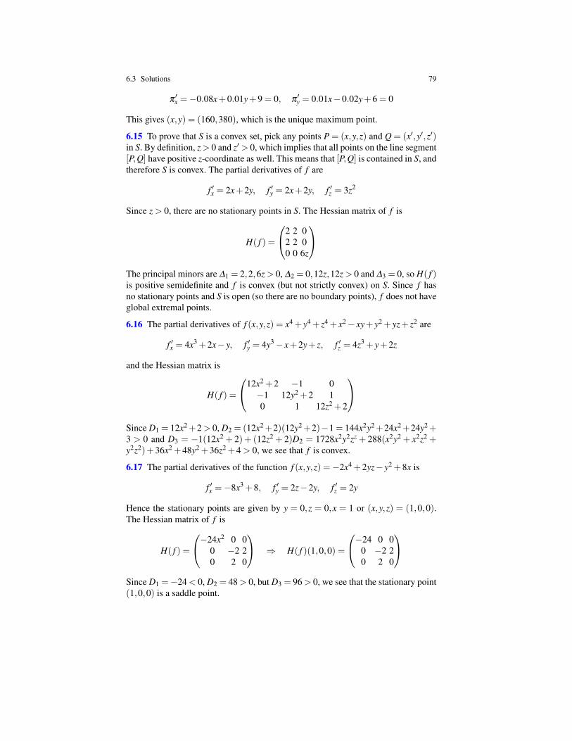
6.3 Solutions 79
π′x =−0.08x+0.01y+9 = 0, π
′y = 0.01x−0.02y+6 = 0
This gives (x,y) = (160,380), which is the unique maximum point.
6.15 To prove that S is a convex set, pick any points P = (x,y,z) and Q = (x′,y′,z′)in S. By definition, z> 0 and z′> 0, which implies that all points on the line segment[P,Q] have positive z-coordinate as well. This means that [P,Q] is contained in S, andtherefore S is convex. The partial derivatives of f are
f ′x = 2x+2y, f ′y = 2x+2y, f ′z = 3z2
Since z > 0, there are no stationary points in S. The Hessian matrix of f is
H( f ) =
2 2 02 2 00 0 6z
The principal minors are ∆1 = 2,2,6z > 0, ∆2 = 0,12z,12z > 0 and ∆3 = 0, so H( f )is positive semidefinite and f is convex (but not strictly convex) on S. Since f hasno stationary points and S is open (so there are no boundary points), f does not haveglobal extremal points.
6.16 The partial derivatives of f (x,y,z) = x4 + y4 + z4 + x2− xy+ y2 + yz+ z2 are
f ′x = 4x3 +2x− y, f ′y = 4y3− x+2y+ z, f ′z = 4z3 + y+2z
and the Hessian matrix is
H( f ) =
12x2 +2 −1 0−1 12y2 +2 10 1 12z2 +2
Since D1 = 12x2+2 > 0, D2 = (12x2+2)(12y2+2)−1 = 144x2y2+24x2+24y2+3 > 0 and D3 = −1(12x2 + 2)+ (12z2 + 2)D2 = 1728x2y2zz + 288(x2y2 + x2z2 +y2z2)+36x2 +48y2 +36z2 +4 > 0, we see that f is convex.
6.17 The partial derivatives of the function f (x,y,z) =−2x4 +2yz− y2 +8x is
f ′x =−8x3 +8, f ′y = 2z−2y, f ′z = 2y
Hence the stationary points are given by y = 0,z = 0,x = 1 or (x,y,z) = (1,0,0).The Hessian matrix of f is
H( f ) =
−24x2 0 00 −2 20 2 0
⇒ H( f )(1,0,0) =
−24 0 00 −2 20 2 0
Since D1 =−24 < 0, D2 = 48 > 0, but D3 = 96 > 0, we see that the stationary point(1,0,0) is a saddle point.
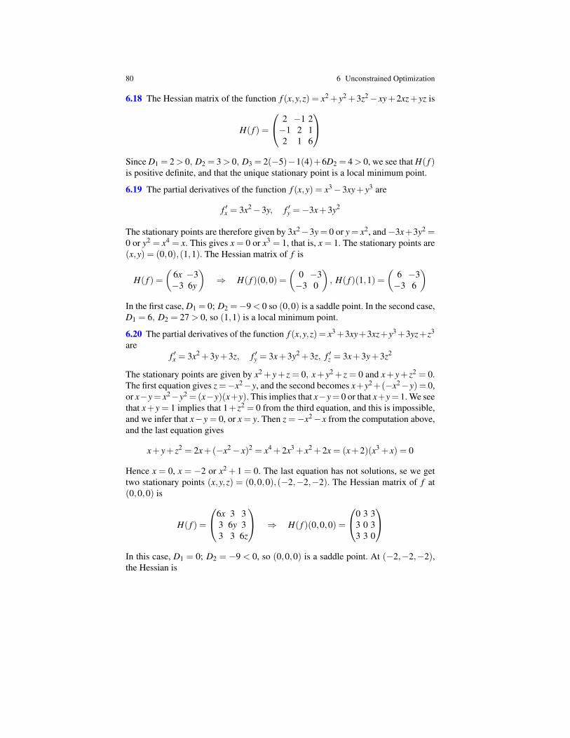
80 6 Unconstrained Optimization
6.18 The Hessian matrix of the function f (x,y,z) = x2 + y2 +3z2− xy+2xz+ yz is
H( f ) =
2 −1 2−1 2 12 1 6
Since D1 = 2 > 0, D2 = 3 > 0, D3 = 2(−5)−1(4)+6D2 = 4 > 0, we see that H( f )is positive definite, and that the unique stationary point is a local minimum point.
6.19 The partial derivatives of the function f (x,y) = x3−3xy+ y3 are
f ′x = 3x2−3y, f ′y =−3x+3y2
The stationary points are therefore given by 3x2−3y = 0 or y = x2, and−3x+3y2 =0 or y2 = x4 = x. This gives x = 0 or x3 = 1, that is, x = 1. The stationary points are(x,y) = (0,0),(1,1). The Hessian matrix of f is
H( f ) =(
6x −3−3 6y
)⇒ H( f )(0,0) =
(0 −3−3 0
), H( f )(1,1) =
(6 −3−3 6
)In the first case, D1 = 0; D2 =−9 < 0 so (0,0) is a saddle point. In the second case,D1 = 6, D2 = 27 > 0, so (1,1) is a local minimum point.
6.20 The partial derivatives of the function f (x,y,z) = x3+3xy+3xz+y3+3yz+z3
aref ′x = 3x2 +3y+3z, f ′y = 3x+3y2 +3z, f ′z = 3x+3y+3z2
The stationary points are given by x2 + y+ z = 0, x+ y2 + z = 0 and x+ y+ z2 = 0.The first equation gives z=−x2−y, and the second becomes x+y2+(−x2−y) = 0,or x−y= x2−y2 =(x−y)(x+y). This implies that x−y= 0 or that x+y= 1. We seethat x+y = 1 implies that 1+ z2 = 0 from the third equation, and this is impossible,and we infer that x−y = 0, or x = y. Then z =−x2−x from the computation above,and the last equation gives
x+ y+ z2 = 2x+(−x2− x)2 = x4 +2x3 + x2 +2x = (x+2)(x3 + x) = 0
Hence x = 0, x = −2 or x2 + 1 = 0. The last equation has not solutions, se we gettwo stationary points (x,y,z) = (0,0,0),(−2,−2,−2). The Hessian matrix of f at(0,0,0) is
H( f ) =
6x 3 33 6y 33 3 6z
⇒ H( f )(0,0,0) =
0 3 33 0 33 3 0
In this case, D1 = 0; D2 = −9 < 0, so (0,0,0) is a saddle point. At (−2,−2,−2),the Hessian is
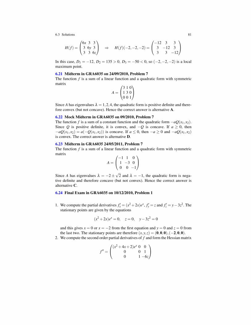
6.3 Solutions 81
H( f ) =
6x 3 33 6y 33 3 6z
⇒ H( f )(−2,−2,−2) =
−12 3 33 −12 33 3 −12
In this case, D1 = −12, D2 = 135 > 0, D3 = −50 < 0, so (−2,−2,−2) is a localmaximum point.
6.21 Midterm in GRA6035 on 24/09/2010, Problem 7The function f is a sum of a linear function and a quadratic form with symmetricmatrix
A =
3 1 01 3 00 0 1
Since A has eigenvalues λ = 1,2,4, the quadratic form is positive definite and there-fore convex (but not concave). Hence the correct answer is alternative A.
6.22 Mock Midterm in GRA6035 on 09/2010, Problem 7The function f is a sum of a constant function and the quadratic form −aQ(x1,x2).Since Q is positive definite, it is convex, and −Q is concave. If a ≥ 0, then−aQ(x1,x2) = a(−Q(x1,x2)) is concave. If a ≤ 0, then −a ≥ 0 and −aQ(x1,x2)is convex. The correct answer is alternative D.
6.23 Midterm in GRA6035 24/05/2011, Problem 7The function f is a sum of a linear function and a quadratic form with symmetricmatrix
A =
−1 1 01 −3 00 0 −1
Since A has eigenvalues λ = −2±
√2 and λ = −1, the quadratic form is nega-
tive definite and therefore concave (but not convex). Hence the correct answer isalternative C.
6.24 Final Exam in GRA6035 on 10/12/2010, Problem 1
1. We compute the partial derivatives f ′x = (x2 +2x)ex, f ′y = z and f ′z = y−3z2. Thestationary points are given by the equations
(x2 +2x)ex = 0, z = 0, y−3z2 = 0
and this gives x = 0 or x = −2 from the first equation and y = 0 and z = 0 fromthe last two. The stationary points are therefore (x,y,z) = (0,0,0),(−2,0,0).
2. We compute the second order partial derivatives of f and form the Hessian matrix
f ′′ =
(x2 +4x+2)ex 0 00 0 10 1 −6z
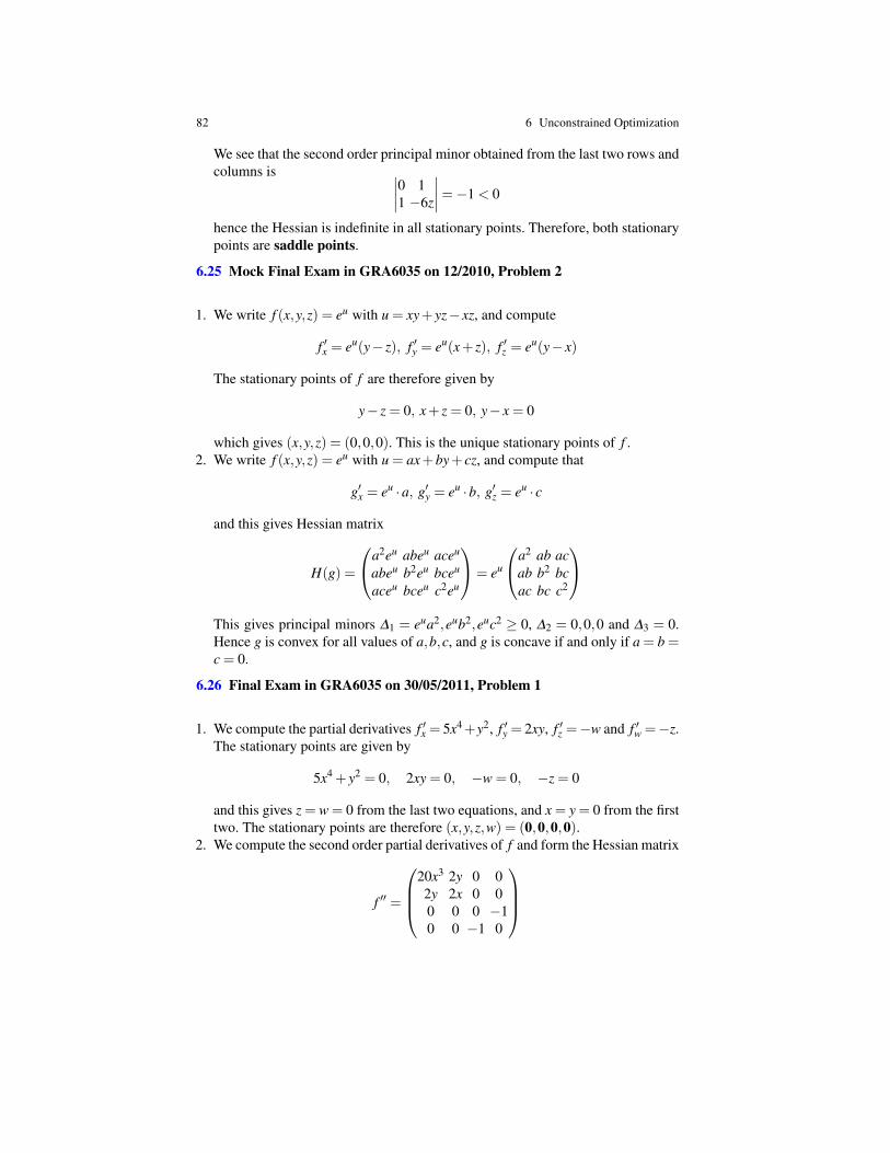
82 6 Unconstrained Optimization
We see that the second order principal minor obtained from the last two rows andcolumns is ∣∣∣∣0 1
1 −6z
∣∣∣∣=−1 < 0
hence the Hessian is indefinite in all stationary points. Therefore, both stationarypoints are saddle points.
6.25 Mock Final Exam in GRA6035 on 12/2010, Problem 2
1. We write f (x,y,z) = eu with u = xy+ yz− xz, and compute
f ′x = eu(y− z), f ′y = eu(x+ z), f ′z = eu(y− x)
The stationary points of f are therefore given by
y− z = 0, x+ z = 0, y− x = 0
which gives (x,y,z) = (0,0,0). This is the unique stationary points of f .2. We write f (x,y,z) = eu with u = ax+by+ cz, and compute that
g′x = eu ·a, g′y = eu ·b, g′z = eu · c
and this gives Hessian matrix
H(g) =
a2eu abeu aceu
abeu b2eu bceu
aceu bceu c2eu
= eu
a2 ab acab b2 bcac bc c2
This gives principal minors ∆1 = eua2,eub2,euc2 ≥ 0, ∆2 = 0,0,0 and ∆3 = 0.Hence g is convex for all values of a,b,c, and g is concave if and only if a = b =c = 0.
6.26 Final Exam in GRA6035 on 30/05/2011, Problem 1
1. We compute the partial derivatives f ′x = 5x4+y2, f ′y = 2xy, f ′z =−w and f ′w =−z.The stationary points are given by
5x4 + y2 = 0, 2xy = 0, −w = 0, −z = 0
and this gives z = w = 0 from the last two equations, and x = y = 0 from the firsttwo. The stationary points are therefore (x,y,z,w) = (0,0,0,0).
2. We compute the second order partial derivatives of f and form the Hessian matrix
f ′′ =
20x3 2y 0 02y 2x 0 00 0 0 −10 0 −1 0
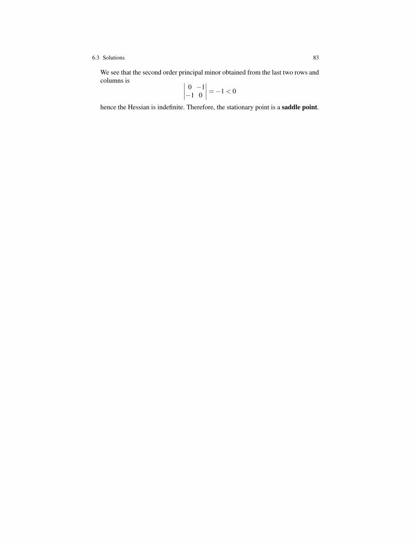
6.3 Solutions 83
We see that the second order principal minor obtained from the last two rows andcolumns is ∣∣∣∣ 0 −1
−1 0
∣∣∣∣=−1 < 0
hence the Hessian is indefinite. Therefore, the stationary point is a saddle point.

Previous: Lecture 6 Contents Next: Lecture 8
Lecture 7Constrained Optimization and First OrderConditions
7.1 Main concepts
A constrained optimization problem is called a Lagrange problem if it has equalityconstraints, and a Kuhn-Tucker problem if it has closed inequality constraints. ALagrange problem can be written in the standard form
max/min f (x) when
g1(x) = a1
g2(x) = a2...gm(x) = am
where f ,g1, . . . ,gm are functions in n variables and a1, . . . ,am are given numbers,and a Kuhn-Tucker problem can be written in standard form as
max f (x) when
g1(x)≤ a1
g2(x)≤ a2...gm(x)≤ am
Given any Lagrange or Kuhn-Tucker problem in standard form, we can constructthe Lagrangian function
L (x1, . . . ,xn,λ1, . . . ,λm) = f (x)−λ1g1(x)−λ2g2(x)−·· ·−λmgm(x)
in the n+m variables x1, . . . ,xn,λ1, . . . ,λm. The variables λ1, . . . ,λm are called theLagrange multipliers. The first order conditions (FOC) of the Lagrange or Kuhn-Tucker problem are the conditions
L ′x1= L ′
x2= · · ·= L ′
xn = 0
Problems Lecture 7 Solutions
86 7 Constrained Optimization and First Order Conditions
Proposition 7.1. If the Lagrange problem has a solution x∗ and this solution satisfythe NDCQ condition
rk
∂g1∂x1
∂g1∂x2
. . . ∂g1∂xn
∂g2∂x1
∂g2∂x2
. . . ∂g2∂xn
. . .. . .
.... . .
∂gm∂x1
∂gm∂x2
. . . ∂gm∂xn
= m
at x∗, then there are unique Lagrange multipliers λ1, . . . ,λm such that (x∗,λ1, . . . ,λm)satisfy the FOC’s and the constraints.
In a Kuhn-Tucker problem, there are additional conditions called complementaryslackness conditions (CSC), and they have the form
λi ≥ 0 and λi(gi(x)−ai) = 0
for i = 1,2, . . .m. We say that the constraint gi(x)≤ ai is binding at x if gi(x) = ai,and non-binding if gi(x) < ai, and the CSC’s say that λ1,λ2, . . . ,λm ≥ 0 and thatλi = 0 for each constraint that is non-binding.
Proposition 7.2. If the Kuhn-Tucker problem has a solution x∗ and this solutionsatisfy the NDCQ condition rkA = k, where A is the submatrix of
∂g1∂x1
∂g1∂x2
. . . ∂g1∂xn
∂g2∂x1
∂g2∂x2
. . . ∂g2∂xn
. . .. . .
.... . .
∂gm∂x1
∂gm∂x2
. . . ∂gm∂xn
consisting of the k rows corresponding to binding constraints at x∗, then there areunique Lagrange multipliers λ1, . . . ,λm such that (x∗,λ1, . . . ,λm) satisfy the FOC’s,the CSC’s and the constraints.
The candidates for max/min in a Lagrange problem are the solutions of the La-grange conditions (FOC’s and constraints) and the points where the NDCQ fails.The candidates for max in a Kuhn-Tucker problem are the solutions of the Kuhn-Tucker conditions (FOC’s, CSC’s and constraints) and the points where NDCQ fails.
A subset D of Rn is called closed if it contains all its boundary points, and openif it does not contain any of its boundary points. A boundary point of D is a pointsuch that any neighbourhood around it contains both points in D and points outsideD. The set of admissible point in a Lagrange or Kuhn-Tucker problem is closed.
The set D is called bounded if there are numbers a1 ≤ b1, a2 ≤ b2, . . . ,an ≤ bn(which are assumed to be finite) such that all points (x1,x2, . . . ,xn) in D satisfies
a1 ≤ x1 ≤ b1, a2 ≤ x2 ≤ b2, . . . , an ≤ xn ≤ bn
7.2 Problems 87
In other words, D is bounded if and only if D is contained in a finite n-dimensionalbox K = [a1,b1]× [a2,b2]×·· ·× [an,bn]. If D is both closed and bounded, it is calleda compact set.
Theorem 7.1 (Weierstrass’ Extreme Value Theorem). If f is a continuous func-tion defined on a compact set, then f has a maximum and a minimum value.
7.2 Problems
7.1. Sketch each set and determine if it is open, closed, bounded or convex:
1. {(x,y) : x2 + y2 < 2}2. {(x,y) : x2 + y2 > 8}3. {(x,y) : xy≤ 1}4. {(x,y) : x≥ 0,y≥ 0}5. {(x,y) : x≥ 0,y≥ 0,xy≥ 1}6. {(x,y) :
√x+√
y≤ 2}
7.2. Use the Lagrange conditions to find candidates for solution of the Lagrangeproblem
max f (x,y) = xy subject to x+4y = 16
7.3. Use the Lagrange conditions to find candidates for solution of the Lagrangeproblem
max f (x,y) = x2y subject to 2x2 + y2 = 3
7.4. Use the Lagrange conditions to find candidates for solution of the Lagrangeproblem
max f (x,y,z) = xyz subject to
{x2 + y2 = 1x+ z = 1
7.5. Use the Lagrange conditions to find candidates for solution of the Lagrangeproblem
max/min f (x,y,z) = x+ y+ z2 subject to
{x2 + y2 + z2 = 1y = 0
7.6. Use the Lagrange conditions to find candidates for solution of the Lagrangeproblem
max f (x,y,z) = xz+ yz subject to
{y2 + z2 = 1xz = 3
7.7. Use the Lagrange conditions to find candidates for solution of the Lagrangeproblem
88 7 Constrained Optimization and First Order Conditions
max f (x,y,z) = x+4y+ z subject to
{x2 + y2 + z2 = 216x+2y+3z = 0
7.8. Use the Kuhn-Tucker conditions to find candidates for solution of the Kuhn-Tucker problem
max f (x,y) = xy subject to x2 + y2 ≤ 1
7.9. Use the Kuhn-Tucker conditions to find candidates for solution of the Kuhn-Tucker problem
max f (x,y,z) = xyz subject to
x+ y+ z≤ 1x≥ 0y≥ 0z≥ 0
7.10. Use the Lagrange conditions to find candidates for solution of the Lagrangeproblem
max f (x,y,z) = ex + y+ z subject to
{x2 + y2 + z2 = 1x+ y+ z = 1
7.11. Final Exam in GRA6035 on 06/02/2012, Problem 4aWe consider the optimization problem
min x2 + y2 + z2 subject to 2x2 +6y2 +3z2 ≥ 36
Write down the first order conditions and the complementary slackness conditionsfor the optimization problem. Find all admissible points that satisfy the first orderconditions and the complementary slackness conditions, and write down the valueof λ for each of these points.
7.3 Solutions
7.1 We see that the sets have the following types:
1. The set {(x,y) : x2 + y2 < 2} is convex, open and bounded, but not closed.2. The set {(x,y) : x2 + y2 > 8} is open, but not closed, bounded or convex.3. The set {(x,y) : xy≤ 1} is closed, but not open, bounded or convex.4. The set {(x,y) : x≥ 0,y≥ 0} is closed and convex, but not open or bounded.5. The set {(x,y) : x ≥ 0,y ≥ 0,xy ≥ 1} is closed and convex, but not open or
bounded.6. The set {(x,y) :
√x+√
y≤ 2} is closed and bounded, but not open or convex.
7.2 The Lagrangian is given by L = xy−λ (x+4y), and we have FOC’s
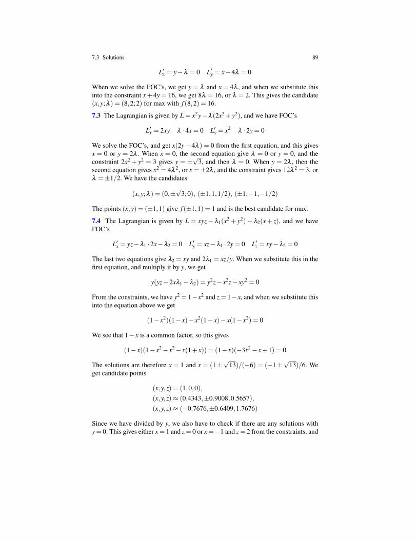
7.3 Solutions 89
L′x = y−λ = 0 L′y = x−4λ = 0
When we solve the FOC’s, we get y = λ and x = 4λ , and when we substitute thisinto the constraint x+4y = 16, we get 8λ = 16, or λ = 2. This gives the candidate(x,y;λ ) = (8,2;2) for max with f (8,2) = 16.
7.3 The Lagrangian is given by L = x2y−λ (2x2 + y2), and we have FOC’s
L′x = 2xy−λ ·4x = 0 L′y = x2−λ ·2y = 0
We solve the FOC’s, and get x(2y−4λ ) = 0 from the first equation, and this givesx = 0 or y = 2λ . When x = 0, the second equation give λ = 0 or y = 0, and theconstraint 2x2 + y2 = 3 gives y = ±
√3, and then λ = 0. When y = 2λ , then the
second equation gives x2 = 4λ 2, or x =±2λ , and the constraint gives 12λ 2 = 3, orλ =±1/2. We have the candidates
(x,y;λ ) = (0,±√
3;0), (±1,1,1/2), (±1,−1,−1/2)
The points (x,y) = (±1,1) give f (±1,1) = 1 and is the best candidate for max.
7.4 The Lagrangian is given by L = xyz− λ1(x2 + y2)− λ2(x+ z), and we haveFOC’s
L′x = yz−λ1 ·2x−λ2 = 0 L′y = xz−λ1 ·2y = 0 L′z = xy−λ2 = 0
The last two equations give λ2 = xy and 2λ1 = xz/y. When we substitute this in thefirst equation, and multiply it by y, we get
y(yz−2xλ1−λ2) = y2z− x2z− xy2 = 0
From the constraints, we have y2 = 1−x2 and z = 1−x, and when we substitute thisinto the equation above we get
(1− x2)(1− x)− x2(1− x)− x(1− x2) = 0
We see that 1− x is a common factor, so this gives
(1− x)(1− x2− x2− x(1+ x)) = (1− x)(−3x2− x+1) = 0
The solutions are therefore x = 1 and x = (1±√
13)/(−6) = (−1±√
13)/6. Weget candidate points
(x,y,z) = (1,0,0),(x,y,z)≈ (0.4343,±0.9008,0.5657),(x,y,z)≈ (−0.7676,±0.6409,1.7676)
Since we have divided by y, we also have to check if there are any solutions withy= 0: This gives either x= 1 and z= 0 or x=−1 and z= 2 from the constraints, and
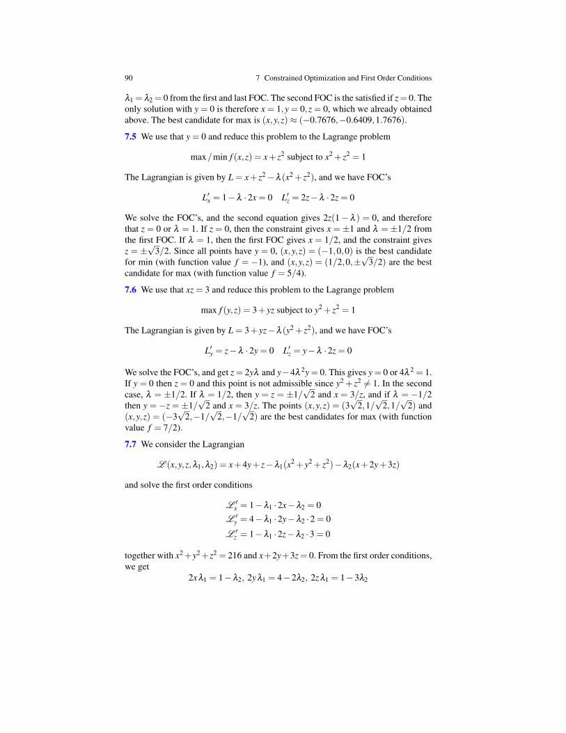
90 7 Constrained Optimization and First Order Conditions
λ1 = λ2 = 0 from the first and last FOC. The second FOC is the satisfied if z= 0. Theonly solution with y = 0 is therefore x = 1,y = 0,z = 0, which we already obtainedabove. The best candidate for max is (x,y,z)≈ (−0.7676,−0.6409,1.7676).
7.5 We use that y = 0 and reduce this problem to the Lagrange problem
max/min f (x,z) = x+ z2 subject to x2 + z2 = 1
The Lagrangian is given by L = x+ z2−λ (x2 + z2), and we have FOC’s
L′x = 1−λ ·2x = 0 L′z = 2z−λ ·2z = 0
We solve the FOC’s, and the second equation gives 2z(1− λ ) = 0, and thereforethat z = 0 or λ = 1. If z = 0, then the constraint gives x = ±1 and λ = ±1/2 fromthe first FOC. If λ = 1, then the first FOC gives x = 1/2, and the constraint givesz = ±
√3/2. Since all points have y = 0, (x,y,z) = (−1,0,0) is the best candidate
for min (with function value f = −1), and (x,y,z) = (1/2,0,±√
3/2) are the bestcandidate for max (with function value f = 5/4).
7.6 We use that xz = 3 and reduce this problem to the Lagrange problem
max f (y,z) = 3+ yz subject to y2 + z2 = 1
The Lagrangian is given by L = 3+ yz−λ (y2 + z2), and we have FOC’s
L′y = z−λ ·2y = 0 L′z = y−λ ·2z = 0
We solve the FOC’s, and get z = 2yλ and y−4λ 2y = 0. This gives y = 0 or 4λ 2 = 1.If y = 0 then z = 0 and this point is not admissible since y2 + z2 6= 1. In the secondcase, λ = ±1/2. If λ = 1/2, then y = z = ±1/
√2 and x = 3/z, and if λ = −1/2
then y = −z = ±1/√
2 and x = 3/z. The points (x,y,z) = (3√
2,1/√
2,1/√
2) and(x,y,z) = (−3
√2,−1/
√2,−1/
√2) are the best candidates for max (with function
value f = 7/2).
7.7 We consider the Lagrangian
L (x,y,z,λ1,λ2) = x+4y+ z−λ1(x2 + y2 + z2)−λ2(x+2y+3z)
and solve the first order conditions
L ′x = 1−λ1 ·2x−λ2 = 0
L ′y = 4−λ1 ·2y−λ2 ·2 = 0
L ′z = 1−λ1 ·2z−λ2 ·3 = 0
together with x2+y2+z2 = 216 and x+2y+3z = 0. From the first order conditions,we get
2xλ1 = 1−λ2, 2yλ1 = 4−2λ2, 2zλ1 = 1−3λ2
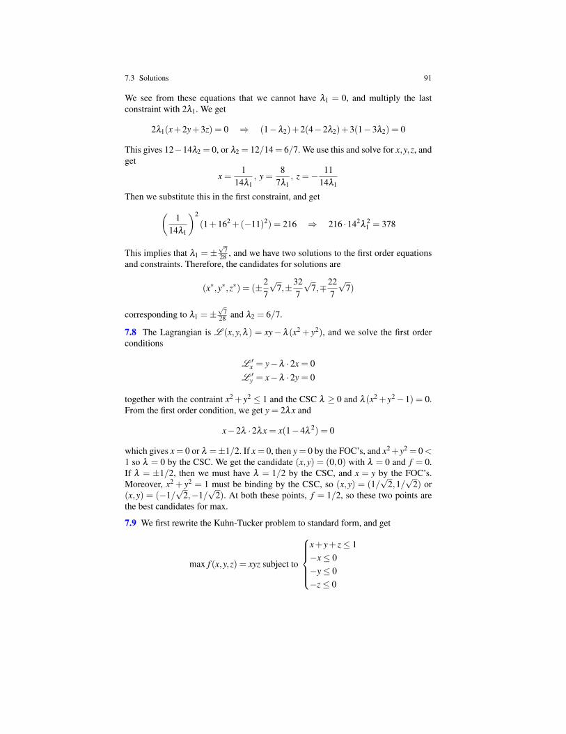
7.3 Solutions 91
We see from these equations that we cannot have λ1 = 0, and multiply the lastconstraint with 2λ1. We get
2λ1(x+2y+3z) = 0 ⇒ (1−λ2)+2(4−2λ2)+3(1−3λ2) = 0
This gives 12−14λ2 = 0, or λ2 = 12/14 = 6/7. We use this and solve for x,y,z, andget
x =1
14λ1, y =
87λ1
, z =− 1114λ1
Then we substitute this in the first constraint, and get(1
14λ1
)2
(1+162 +(−11)2) = 216 ⇒ 216 ·142λ
21 = 378
This implies that λ1 = ±√
728 , and we have two solutions to the first order equations
and constraints. Therefore, the candidates for solutions are
(x∗,y∗,z∗) = (±27
√7,±32
7
√7,∓22
7
√7)
corresponding to λ1 =±√
728 and λ2 = 6/7.
7.8 The Lagrangian is L (x,y,λ ) = xy− λ (x2 + y2), and we solve the first orderconditions
L ′x = y−λ ·2x = 0
L ′y = x−λ ·2y = 0
together with the contraint x2 + y2 ≤ 1 and the CSC λ ≥ 0 and λ (x2 + y2−1) = 0.From the first order condition, we get y = 2λx and
x−2λ ·2λx = x(1−4λ2) = 0
which gives x = 0 or λ =±1/2. If x = 0, then y = 0 by the FOC’s, and x2+y2 = 0 <1 so λ = 0 by the CSC. We get the candidate (x,y) = (0,0) with λ = 0 and f = 0.If λ = ±1/2, then we must have λ = 1/2 by the CSC, and x = y by the FOC’s.Moreover, x2 + y2 = 1 must be binding by the CSC, so (x,y) = (1/
√2,1/√
2) or(x,y) = (−1/
√2,−1/
√2). At both these points, f = 1/2, so these two points are
the best candidates for max.
7.9 We first rewrite the Kuhn-Tucker problem to standard form, and get
max f (x,y,z) = xyz subject to
x+ y+ z≤ 1−x≤ 0−y≤ 0−z≤ 0
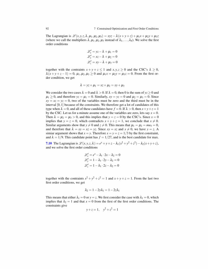
92 7 Constrained Optimization and First Order Conditions
The Lagrangian is L (x,y,z,λ ,µ1,µ2,µ3) = xyz− λ (x+ y+ z)+ µ1x+ µ2y+ µ3z(where we call the multipliers λ ,µ1,µ2,µ3 instead of λ1, . . . ,λ4). We solve the firstorder conditions
L ′x = yz−λ +µ1 = 0
L ′y = xz−λ +µ2 = 0
L ′z = xy−λ +µ3 = 0
together with the contraints x + y + z ≤ 1 and x,y,z ≥ 0 and the CSC’s λ ≥ 0,λ (x+ y+ z− 1) = 0, µ1,µ2,µ3 ≥ 0 and µ1x = µ2y = µ3z = 0. From the first or-der condition, we get
λ = yz+µ1 = xz+µ2 = xy+µ3
We consider the two cases λ = 0 and λ > 0. If λ = 0, then 0 is the sum of yz≥ 0 andµ1 ≥ 0, and therefore yz = µ1 = 0. Similarly, xy = yz = 0 and µ2 = µ3 = 0. Sincexy = xz = yz = 0, two of the variables must be zero and the third must be in theinterval [0,1] because of the constraints. We therefore get a lot of candidates of thistype when λ = 0, and all of these candidates have f = 0. If λ > 0, then x+y+z = 1by the CSC. Let us for a minute assume one of the variables are zero, lets say x = 0.Then λ = µ2 = µ3 > 0, and this implies that y = z = 0 by the CSC’s. Since x = 0implies that y = z = 0, which contradicts x+ y+ z = 1, we conclude that x 6= 0.Similar arguments show that y 6= 0 and z 6= 0. This means that µ1 = µ2 = mu3 = 0,and therefore that λ = xy = xz = yz. Since xy = xz and x 6= 0, we have y = z. Asimiar argument shows that x = y. Therefore x = y = z = 1/3 by the first constraint,and λ = 1/9. This candidate point has f = 1/27, and is the best candidate for max.
7.10 The Lagrangian is L (x,y,z,λ ) = ex +y+ z−λ1(x2 +y2 + z2)−λ2(x+y+ z),and we solve the first order conditions
L ′x = ex−λ1 ·2x−λ2 = 0
L ′y = 1−λ1 ·2y−λ2 = 0
L ′z = 1−λ1 ·2z−λ2 = 0
together with the contraints x2 + y2 + z2 = 1 and x+ y+ z = 1. From the last twofirst order conditions, we get
λ2 = 1−2yλ1 = 1−2zλ1
This means that either λ1 = 0 or y = z. We first consider the case with λ1 = 0, whichimplies that λ2 = 1 and that x = 0 from the first of the first order conditions. Theconstraints give
y+ z = 1, y2 + z2 = 1
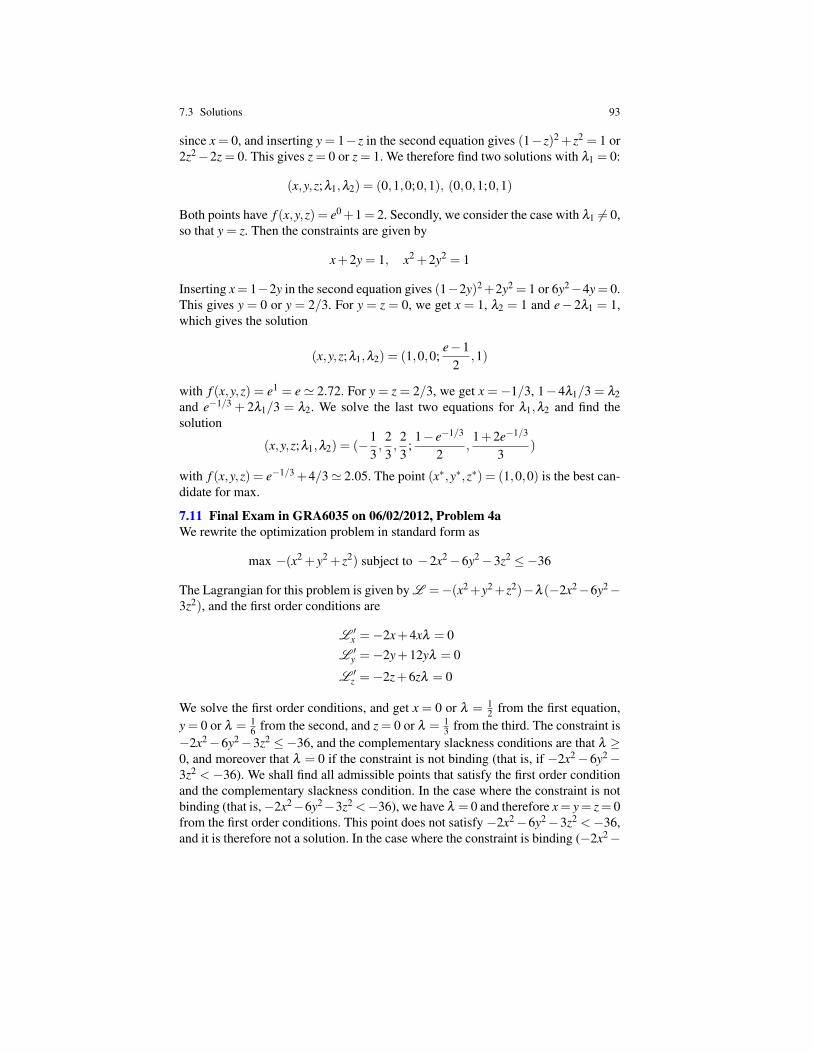
7.3 Solutions 93
since x = 0, and inserting y = 1− z in the second equation gives (1− z)2 + z2 = 1 or2z2−2z = 0. This gives z = 0 or z = 1. We therefore find two solutions with λ1 = 0:
(x,y,z;λ1,λ2) = (0,1,0;0,1), (0,0,1;0,1)
Both points have f (x,y,z) = e0+1 = 2. Secondly, we consider the case with λ1 6= 0,so that y = z. Then the constraints are given by
x+2y = 1, x2 +2y2 = 1
Inserting x= 1−2y in the second equation gives (1−2y)2+2y2 = 1 or 6y2−4y= 0.This gives y = 0 or y = 2/3. For y = z = 0, we get x = 1, λ2 = 1 and e− 2λ1 = 1,which gives the solution
(x,y,z;λ1,λ2) = (1,0,0;e−1
2,1)
with f (x,y,z) = e1 = e' 2.72. For y = z = 2/3, we get x =−1/3, 1−4λ1/3 = λ2and e−1/3 + 2λ1/3 = λ2. We solve the last two equations for λ1,λ2 and find thesolution
(x,y,z;λ1,λ2) = (−13,
23,
23
;1− e−1/3
2,
1+2e−1/3
3)
with f (x,y,z) = e−1/3 +4/3' 2.05. The point (x∗,y∗,z∗) = (1,0,0) is the best can-didate for max.
7.11 Final Exam in GRA6035 on 06/02/2012, Problem 4aWe rewrite the optimization problem in standard form as
max −(x2 + y2 + z2) subject to −2x2−6y2−3z2 ≤−36
The Lagrangian for this problem is given by L =−(x2+y2+z2)−λ (−2x2−6y2−3z2), and the first order conditions are
L ′x =−2x+4xλ = 0
L ′y =−2y+12yλ = 0
L ′z =−2z+6zλ = 0
We solve the first order conditions, and get x = 0 or λ = 12 from the first equation,
y = 0 or λ = 16 from the second, and z = 0 or λ = 1
3 from the third. The constraint is−2x2−6y2−3z2 ≤−36, and the complementary slackness conditions are that λ ≥0, and moreover that λ = 0 if the constraint is not binding (that is, if −2x2−6y2−3z2 <−36). We shall find all admissible points that satisfy the first order conditionand the complementary slackness condition. In the case where the constraint is notbinding (that is,−2x2−6y2−3z2 <−36), we have λ = 0 and therefore x= y= z= 0from the first order conditions. This point does not satisfy −2x2−6y2−3z2 <−36,and it is therefore not a solution. In the case where the constraint is binding (−2x2−
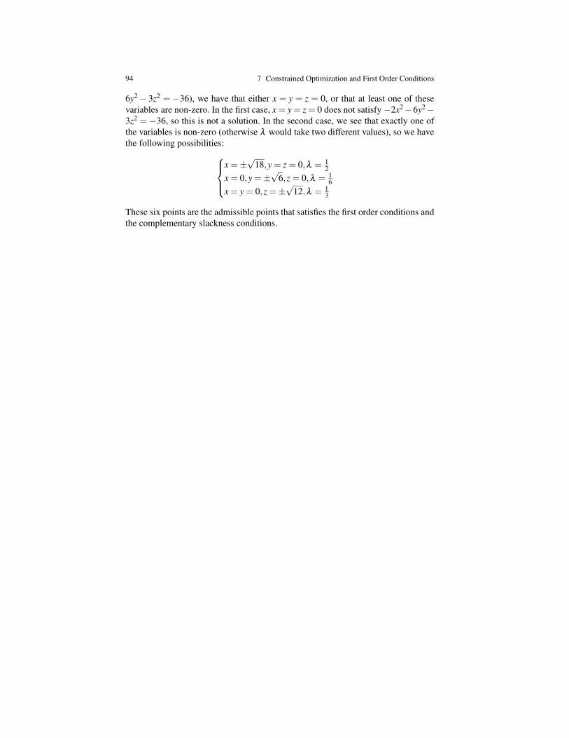
94 7 Constrained Optimization and First Order Conditions
6y2− 3z2 = −36), we have that either x = y = z = 0, or that at least one of thesevariables are non-zero. In the first case, x = y = z = 0 does not satisfy −2x2−6y2−3z2 = −36, so this is not a solution. In the second case, we see that exactly one ofthe variables is non-zero (otherwise λ would take two different values), so we havethe following possibilities:
x =±√
18,y = z = 0,λ = 12
x = 0,y =±√
6,z = 0,λ = 16
x = y = 0,z =±√
12,λ = 13
These six points are the admissible points that satisfies the first order conditions andthe complementary slackness conditions.
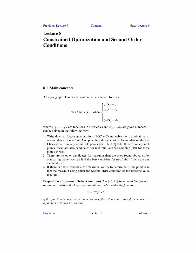
Previous: Lecture 7 Contents Next: Lecture 9
Lecture 8Constrained Optimization and Second OrderConditions
8.1 Main concepts
A Lagrange problem can be written in the standard form as
max/min f (x) when
g1(x) = a1
g2(x) = a2...gm(x) = am
where f ,g1, . . . ,gm are functions in n variables and a1, . . . ,am are given numbers. Itcan be solved in the following way:
1. Write down all Lagrange conditions (FOC + C) and solve them, to obtain a listof candidates for max/min. Compute the value f (x) of each candidate on the list.
2. Check if there are any admissible points where NDCQ fails. If there are any suchpoints, these are also candidates for max/min, and we compute f (x) for thesepoints as well.
3. There are no other candidates for max/min than the ones found above, so bycomparing values we can find the best candidate for max/min (if there are anycandidates).
4. If there is a best candidate for max/min, we try to determine if this point is infact the max/min using either the Second order condition or the Extreme valuetheorem.
Proposition 8.1 (Second Order Condition). Let (x∗;λ ∗) be a candidate for maxor min that satisfies the Lagrange conditions, and consider the function
x 7→L (x,λ ∗)
If this function is concave as a function in x, then x∗ is a max, and if it is convex asa function in x then x∗ is a min.
Problems Lecture 8 Solutions
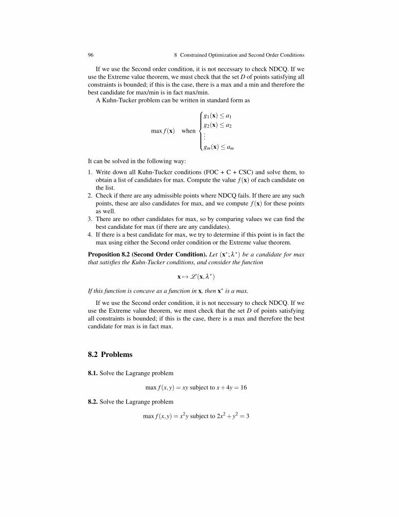
96 8 Constrained Optimization and Second Order Conditions
If we use the Second order condition, it is not necessary to check NDCQ. If weuse the Extreme value theorem, we must check that the set D of points satisfying allconstraints is bounded; if this is the case, there is a max and a min and therefore thebest candidate for max/min is in fact max/min.
A Kuhn-Tucker problem can be written in standard form as
max f (x) when
g1(x)≤ a1
g2(x)≤ a2...gm(x)≤ am
It can be solved in the following way:
1. Write down all Kuhn-Tucker conditions (FOC + C + CSC) and solve them, toobtain a list of candidates for max. Compute the value f (x) of each candidate onthe list.
2. Check if there are any admissible points where NDCQ fails. If there are any suchpoints, these are also candidates for max, and we compute f (x) for these pointsas well.
3. There are no other candidates for max, so by comparing values we can find thebest candidate for max (if there are any candidates).
4. If there is a best candidate for max, we try to determine if this point is in fact themax using either the Second order condition or the Extreme value theorem.
Proposition 8.2 (Second Order Condition). Let (x∗;λ ∗) be a candidate for maxthat satisfies the Kuhn-Tucker conditions, and consider the function
x 7→L (x,λ ∗)
If this function is concave as a function in x, then x∗ is a max.
If we use the Second order condition, it is not necessary to check NDCQ. If weuse the Extreme value theorem, we must check that the set D of points satisfyingall constraints is bounded; if this is the case, there is a max and therefore the bestcandidate for max is in fact max.
8.2 Problems
8.1. Solve the Lagrange problem
max f (x,y) = xy subject to x+4y = 16
8.2. Solve the Lagrange problem
max f (x,y) = x2y subject to 2x2 + y2 = 3
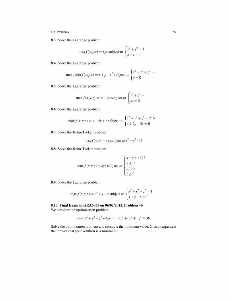
8.2 Problems 97
8.3. Solve the Lagrange problem
max f (x,y,z) = xyz subject to
{x2 + y2 = 1x+ z = 1
8.4. Solve the Lagrange problem
max/min f (x,y,z) = x+ y+ z2 subject to
{x2 + y2 + z2 = 1y = 0
8.5. Solve the Lagrange problem
max f (x,y,z) = xz+ yz subject to
{y2 + z2 = 1xz = 3
8.6. Solve the Lagrange problem
max f (x,y,z) = x+4y+ z subject to
{x2 + y2 + z2 = 216x+2y+3z = 0
8.7. Solve the Kuhn-Tucker problem
max f (x,y) = xy subject to x2 + y2 ≤ 1
8.8. Solve the Kuhn-Tucker problem
max f (x,y,z) = xyz subject to
x+ y+ z≤ 1x≥ 0y≥ 0z≥ 0
8.9. Solve the Lagrange problem
max f (x,y,z) = ex + y+ z subject to
{x2 + y2 + z2 = 1x+ y+ z = 1
8.10. Final Exam in GRA6035 on 06/02/2012, Problem 4bWe consider the optimization problem
min x2 + y2 + z2 subject to 2x2 +6y2 +3z2 ≥ 36
Solve the optimization problem and compute the minimum value. Give an argumentthat proves that your solution is a minimum.
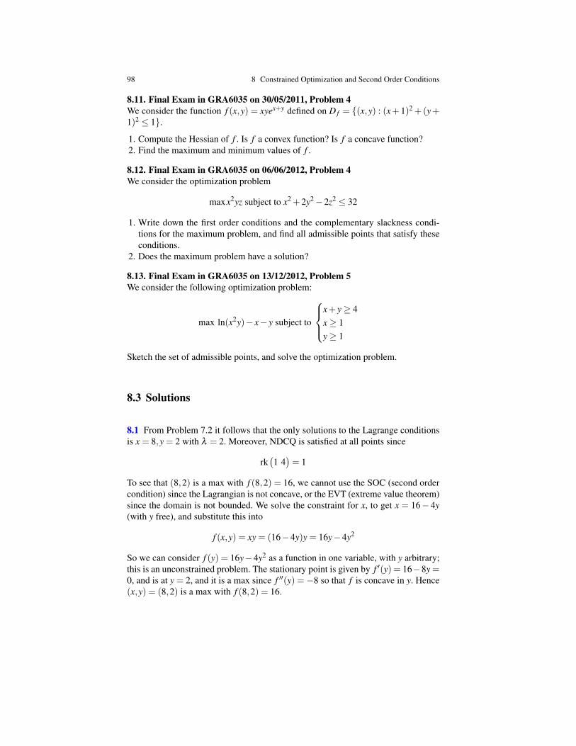
98 8 Constrained Optimization and Second Order Conditions
8.11. Final Exam in GRA6035 on 30/05/2011, Problem 4We consider the function f (x,y) = xyex+y defined on D f = {(x,y) : (x+1)2 +(y+1)2 ≤ 1}.
1. Compute the Hessian of f . Is f a convex function? Is f a concave function?2. Find the maximum and minimum values of f .
8.12. Final Exam in GRA6035 on 06/06/2012, Problem 4We consider the optimization problem
maxx2yz subject to x2 +2y2−2z2 ≤ 32
1. Write down the first order conditions and the complementary slackness condi-tions for the maximum problem, and find all admissible points that satisfy theseconditions.
2. Does the maximum problem have a solution?
8.13. Final Exam in GRA6035 on 13/12/2012, Problem 5We consider the following optimization problem:
max ln(x2y)− x− y subject to
x+ y≥ 4x≥ 1y≥ 1
Sketch the set of admissible points, and solve the optimization problem.
8.3 Solutions
8.1 From Problem 7.2 it follows that the only solutions to the Lagrange conditionsis x = 8,y = 2 with λ = 2. Moreover, NDCQ is satisfied at all points since
rk(1 4)= 1
To see that (8,2) is a max with f (8,2) = 16, we cannot use the SOC (second ordercondition) since the Lagrangian is not concave, or the EVT (extreme value theorem)since the domain is not bounded. We solve the constraint for x, to get x = 16− 4y(with y free), and substitute this into
f (x,y) = xy = (16−4y)y = 16y−4y2
So we can consider f (y) = 16y−4y2 as a function in one variable, with y arbitrary;this is an unconstrained problem. The stationary point is given by f ′(y) = 16−8y =0, and is at y = 2, and it is a max since f ′′(y) =−8 so that f is concave in y. Hence(x,y) = (8,2) is a max with f (8,2) = 16.
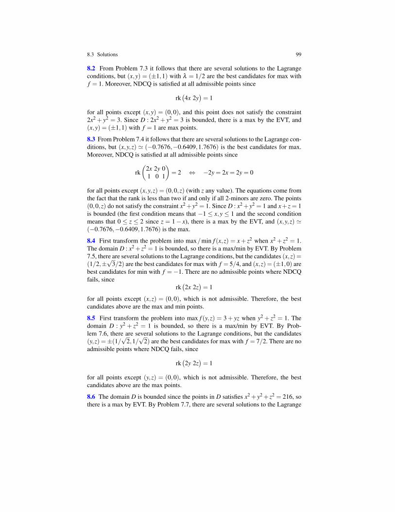
8.3 Solutions 99
8.2 From Problem 7.3 it follows that there are several solutions to the Lagrangeconditions, but (x,y) = (±1,1) with λ = 1/2 are the best candidates for max withf = 1. Moreover, NDCQ is satisfied at all admissible points since
rk(4x 2y
)= 1
for all points except (x,y) = (0,0), and this point does not satisfy the constraint2x2 + y2 = 3. Since D : 2x2 + y2 = 3 is bounded, there is a max by the EVT, and(x,y) = (±1,1) with f = 1 are max points.
8.3 From Problem 7.4 it follows that there are several solutions to the Lagrange con-ditions, but (x,y,z) ' (−0.7676,−0.6409,1.7676) is the best candidates for max.Moreover, NDCQ is satisfied at all admissible points since
rk(
2x 2y 01 0 1
)= 2 ⇔ −2y = 2x = 2y = 0
for all points except (x,y,z) = (0,0,z) (with z any value). The equations come fromthe fact that the rank is less than two if and only if all 2-minors are zero. The points(0,0,z) do not satisfy the constraint x2 +y2 = 1. Since D : x2 +y2 = 1 and x+ z = 1is bounded (the first condition means that −1 ≤ x,y ≤ 1 and the second conditionmeans that 0 ≤ z ≤ 2 since z = 1− x), there is a max by the EVT, and (x,y,z) '(−0.7676,−0.6409,1.7676) is the max.
8.4 First transform the problem into max/min f (x,z) = x+ z2 when x2 + z2 = 1.The domain D : x2 + z2 = 1 is bounded, so there is a max/min by EVT. By Problem7.5, there are several solutions to the Lagrange conditions, but the candidates (x,z)=(1/2,±
√3/2) are the best candidates for max with f = 5/4, and (x,z) = (±1,0) are
best candidates for min with f =−1. There are no admissible points where NDCQfails, since
rk(2x 2z
)= 1
for all points except (x,z) = (0,0), which is not admissible. Therefore, the bestcandidates above are the max and min points.
8.5 First transform the problem into max f (y,z) = 3+ yz when y2 + z2 = 1. Thedomain D : y2 + z2 = 1 is bounded, so there is a max/min by EVT. By Prob-lem 7.6, there are several solutions to the Lagrange conditions, but the candidates(y,z) =±(1/
√2,1/√
2) are the best candidates for max with f = 7/2. There are noadmissible points where NDCQ fails, since
rk(2y 2z
)= 1
for all points except (y,z) = (0,0), which is not admissible. Therefore, the bestcandidates above are the max points.
8.6 The domain D is bounded since the points in D satisfies x2 + y2 + z2 = 216, sothere is a max by EVT. By Problem 7.7, there are several solutions to the Lagrange
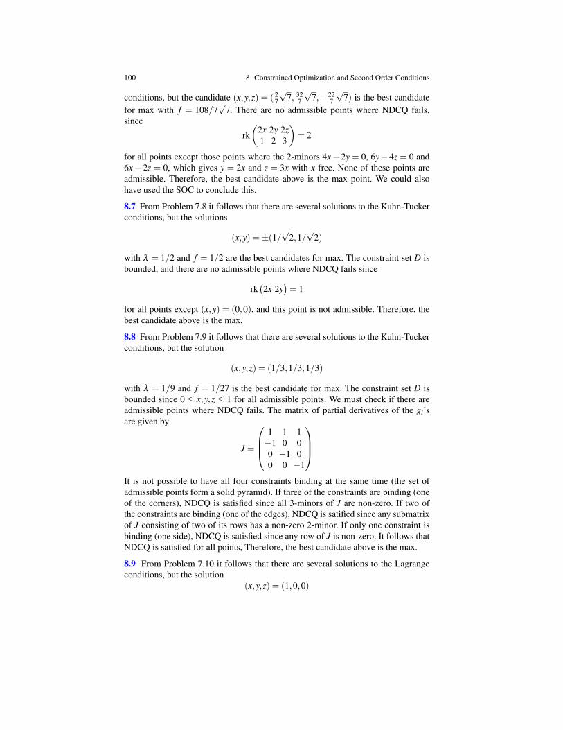
100 8 Constrained Optimization and Second Order Conditions
conditions, but the candidate (x,y,z) = ( 27
√7, 32
7
√7,− 22
7
√7) is the best candidate
for max with f = 108/7√
7. There are no admissible points where NDCQ fails,since
rk(
2x 2y 2z1 2 3
)= 2
for all points except those points where the 2-minors 4x− 2y = 0, 6y− 4z = 0 and6x− 2z = 0, which gives y = 2x and z = 3x with x free. None of these points areadmissible. Therefore, the best candidate above is the max point. We could alsohave used the SOC to conclude this.
8.7 From Problem 7.8 it follows that there are several solutions to the Kuhn-Tuckerconditions, but the solutions
(x,y) =±(1/√
2,1/√
2)
with λ = 1/2 and f = 1/2 are the best candidates for max. The constraint set D isbounded, and there are no admissible points where NDCQ fails since
rk(2x 2y
)= 1
for all points except (x,y) = (0,0), and this point is not admissible. Therefore, thebest candidate above is the max.
8.8 From Problem 7.9 it follows that there are several solutions to the Kuhn-Tuckerconditions, but the solution
(x,y,z) = (1/3,1/3,1/3)
with λ = 1/9 and f = 1/27 is the best candidate for max. The constraint set D isbounded since 0 ≤ x,y,z ≤ 1 for all admissible points. We must check if there areadmissible points where NDCQ fails. The matrix of partial derivatives of the gi’sare given by
J =
1 1 1−1 0 00 −1 00 0 −1
It is not possible to have all four constraints binding at the same time (the set ofadmissible points form a solid pyramid). If three of the constraints are binding (oneof the corners), NDCQ is satisfied since all 3-minors of J are non-zero. If two ofthe constraints are binding (one of the edges), NDCQ is satified since any submatrixof J consisting of two of its rows has a non-zero 2-minor. If only one constraint isbinding (one side), NDCQ is satisfied since any row of J is non-zero. It follows thatNDCQ is satisfied for all points, Therefore, the best candidate above is the max.
8.9 From Problem 7.10 it follows that there are several solutions to the Lagrangeconditions, but the solution
(x,y,z) = (1,0,0)
8.3 Solutions 101
with λ1 = (e−1)/2, λ2 = 1 and f = e is the best candidate for max. The constraintset D is bounded since −1 ≤ x,y,z ≤ 1 for all admissible points. We must check ifthere are admissible points where NDCQ fails. The NDCQ condition
rk(
2x 2y 2z1 1 1
)= 2
is satisfied for all points except where the 2-minors 2x−2y = 2x−2z = 2y−2z = 0,or x = y = z. These are no admissible points with x = y = z, so the best candidateabove is the max.
8.10 Final Exam in GRA6035 on 06/02/2012, Problem 4bWe rewrite the optimization problem in standard form as
max −(x2 + y2 + z2) subject to −2x2−6y2−3z2 ≤−36
By problem 7.10, the best candidate for max is the points (x,y,z) = (0,±√
6,0) withλ = 1/6 and f =−(x2 + y2 + z2) =−6. We consider the Lagrangian
L (x,y,z,1/6) =−(x2 + y2 + z2)−1/6(−2x2−6y2−3z2) =−23
x2− 12
z2
which is clearly concave in (x,y,z). Hence (x,y,z) = (0,±√
6,0) are max pointswith max value f = −6 by the SOC (second order condition). This means that thepoints (x,y,z) = (0,±
√6,0) are min points for the original optimization problem
with minimum value 6.
8.11 Final Exam in GRA6035 on 30/05/2011, Problem 4
1. We compute the partial derivatives f (x,y) = xyex+y, and find that
f ′x = yex+y + xyex+y = (y+ xy)exy, f ′y = xex+y + xyex+y = (x+ xy)exy
The first among the second order partial derivative is given by
f ′′xx = yex+y +(y+ xy)ex+y = (2y+ xy)ex+y = (x+2)yex+y
The other second order partial derivatives can be computed in a similar way, andwe find that the Hessian is given by
H( f )(x,y) =(
(x+2)yex+y (x+1)(y+1)ex+y
(x+1)(y+1)ex+y x(y+2)ex+y
)We compute the principal minors of the Hessian, and we find that the first orderprincipal minors are ∆1 = (x+2)yex+y and ∆1 = x(y+2)ex+y. The second orderprincipal minor is
102 8 Constrained Optimization and Second Order Conditions
D2 = (x+2)yex+y · x(y+2)ex+y− (x+1)2(y+1)2(ex+y)2
= (1− (x+1)2− (y+1)2)e2(x+y)
since the expressions in D2 are (x+2)xy(y+2) = x2y2 +2xy2 +2x2y+4xy and(x+1)2(y+1)2 = (x2 +2x+1)(y2 +2y+1) = x2y2 +2xy2 +2x2y+ x2 +4xy+y2 +2x+2y+1, so that their difference is
(x2y2 +2xy2 +2x2y+4xy)− (x2y2 +2xy2 +2x2y+ x2 +4xy+ y2 +2x+2y+1)
=−x2−2x− y2−2y−1 =−(x2 +2x+1)− (y2 +2y+1)+1
= 1− (x+1)2− (y+1)2
Finally, we have to determine the signs of the principal minors when (x,y) isin the domain of definition D f , given by (x+ 1)2 + (y+ 1)2 ≤ 1. We see thatD2 ≥ 0. Moreover, we notice that D f is the disc inside a circle with radius 1 andwith center (−1,−1). Therefore −2 ≤ x,y ≤ 0 for all points in D f , and ∆1 ≤ 0.It follows that f is a concave function on D f . It is not convex since ∆1 < 0 forsome points in D f (in fact, all points except (−1,0) and (0,−1)).
2. Since D f is closed and bounded, f has maximum and minimum values on D f .We compute the stationary points of f : We have
f ′x = (x+1)yex+y = 0, f ′y = x(y+1)ex+y = 0
and (x,y)= (0,0) and (x,y)= (−1,−1) are the solutions. Hence there is only onestationary point (x,y) = (−1,−1) in D f , and f (−1,−1) = e−2 is the maximumvalue of f since f is concave on D f . The minimum value most occur for (x,y) onthe boundary of D f . We see that f (x,y)≥ 0 for all (x,y) ∈ D f while f (−1,0) =f (0,−1) = 0. Hence f(−1,0) = f(0,−1) = 0 is the minimum value of f .
8.12 Final Exam in GRA6035 on 06/06/2012, Problem 4
1. The Lagrangian for this problem is given by L = x2yz−λ (x2 +2y2−2z2), andthe first order conditions are
L ′x = 2xyz−2xλ = 0
L ′y = x2z−4yλ = 0
L ′z = x2y+4zλ = 0
The complementary slackness conditions are given by λ ≥ 0, and λ = 0 if x2 +2y2−2z2 < 32. Let us find all admissible points satisfying these conditions. Wesolve the first order conditions, and get x = 0 or λ = yz from the first equation. Ifx = 0, then yλ = zλ = 0, so either λ = 0 or λ 6= 0⇒ y = z = 0. In the first case,the constraint gives 2y2−2z2 ≤ 32⇒ y2− z2 ≤ 16. This gives the solution
x = 0, y2− z2 ≤ 16, λ = 0
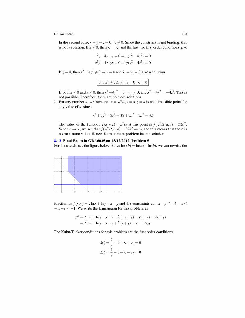
8.3 Solutions 103
In the second case, x = y = z = 0, λ 6= 0. Since the constraint is not binding, thisis not a solution. If x 6= 0, then λ = yz, and the last two first order conditions give
x2z−4y · yz = 0⇒ z(x2−4y2) = 0
x2y+4z · yz = 0⇒ y(x2 +4z2) = 0
If z = 0, then x2 +4z2 6= 0⇒ y = 0 and λ = yz = 0 give a solution
0 < x2 ≤ 32, y = z = 0, λ = 0
If both x 6= 0 and z 6= 0, then x2−4y2 = 0⇒ y 6= 0, and x2 = 4y2 =−4z2. This isnot possible. Therefore, there are no more solutions.
2. For any number a, we have that x =√
32,y = a,z = a is an admissible point forany value of a, since
x2 +2y2−2z2 = 32+2a2−2a2 = 32
The value of the function f (x,y,z) = x2yz at this point is f (√
32,a,a) = 32a2.When a→ ∞, we see that f (
√32,a,a) = 32a2→ ∞, and this means that there is
no maximum value. Hence the maximum problem has no solution.
8.13 Final Exam in GRA6035 on 13/12/2012, Problem 5For the sketch, see the figure below. Since ln(ab) = ln(a)+ ln(b), we can rewrite the
function as f (x,y) = 2lnx+ lny− x− y and the constraints as −x− y ≤ −4,−x ≤−1,−y≤−1. We write the Lagrangian for this problem as
L = 2lnx+ lny− x− y−λ (−x− y)−ν1(−x)−ν2(−y)
= 2lnx+ lny− x− y+λ (x+ y)+ν1x+ν2y
The Kuhn-Tucker conditions for this problem are the first order conditions
L ′x =
2x−1+λ +ν1 = 0
L ′y =
1y−1+λ +ν2 = 0
104 8 Constrained Optimization and Second Order Conditions
the constraints x+ y ≥ 4 and x,y ≥ 1, and the complementary slackness conditionsλ ,ν1,ν2 ≥ 0 and
λ (x+ y−4) = 0, ν1(x−1) = 0, ν2(y−1) = 0
Let us find all solutions of the Kuhn-Tucker conditions: If x = 1, then 1+λ +ν1 = 0by the first FOC and this is not possible (since λ ,ν1 ≥ 0). So we must have x > 1and ν1 = 0. If y = 1, then λ + ν2 = 0 by the second FOC, and this implies thatλ = ν2 = 0 (since λ ,ν2 ≥ 0). Then the first FOC implies that x = 2, and this is notpossible since x+ y ≥ 4. Hence we must also have y > 1 and ν2 = 0. Using theFOC’s, we get
λ = 1− 2x= 1− 1
y
which gives 2/x = 1/y or x = 2y and λ = 1−1/y > 0 since y > 1. This implies thatx+ y = 4, which gives 3y = 4 or y = 4/3, x = 8/3 and λ = 1/4. We conclude thatthere is exactly one solution of the Kuhn-Tucker conditions:
(x,y;λ ,ν1,ν2) = (8/3,4/3;1/4,0,0)
The Lagrangian L =L (x,y;1/4,0,0) = 2lnx+ lny−x−y+(x+y)/4 has Hessian
L ′′ =
(− 2
x2 00 − 1
y2
)
so L is a concave function, since D1 = −2/x2 < 0 and D2 = 2/(x2y2) > 0 (L isonly defined for x,y 6= 0). Therefore (x,y) = (8/3,4/3) is the maximum point.
Previous: Lecture 8 Contents Next: Lecture 10
Lecture 9Envelope Theorems and Bordered Hessians
9.1 Main concepts
Let f (x;a) be a function in n variables that depend on a parameter a, and considerthe unconstrained optimization problem
max/min f (x;a)
for a given value of a.
Theorem 9.1 (Envelope Theorem, Unconstrained case). Assume that the problemhas a solution x∗(a), and consider the optimal value function f ∗(a) = f (x∗(a)).Then we have
d f ∗(a)da
=∂ f∂a
∣∣∣x=x∗(a)
Let f (x;a) be a function in n variables that depend on a parameter a, and considerthe Lagrange problem
max/min f (x;a) when
g1(x;a) = 0g2(x;a) = 0...gm(x;a) = 0
or the Kuhn-Tucker problem
max f (x;a) when
g1(x;a)≤ 0g2(x;a)≤ 0...gm(x;a)≤ 0
Problems Lecture 9 Solutions
106 9 Envelope Theorems and Bordered Hessians
for a given value of a, where the functions g1,g2, . . . ,gm defining the constraintsdepend on the parameter a.
Theorem 9.2 (Envelope Theorem, Constrained case). Assume that the problemhas a solution x∗(a), and consider the optimal value function f ∗(a) = f (x∗(a)).Then we have
d f ∗(a)da
=∂L
∂a
∣∣∣x=x∗(a);λ=λ ∗(a)
where L is the Lagrangian of the problem and λ ∗(a) are the Lagrange multiplierssuch that (x∗(a);λ ∗(a)) satisfy FOC (and CSC in case of a Kuhn-Tucker problem).
Consider a Lagrange or Kuhn-Tucker problem, and assume that (x∗;λ ∗) is asolution of the Lagrange conditions (FOC + C) or the Kuhn-Tucker conditions (FOC+ C + CSC). To find out if x∗ is a local max or local min of the given optimizationproblem, we may use the (m+n)× (m+n) bordered Hessian matrix
B =
(0 J
JT H(L )
)∣∣∣x=x∗;λ=λ ∗
where J is the matrix of all partial derivatives of the functions g1,g2, . . . ,gm definingthe constraints (in the Lagrange case), or only those gi’s that are binding at x∗ (inthe Kuhn-Tucker case), and H(L ) is the Hessian matrix of the Lagrangian L asa function of x (that is, the matrix of the second order derivatives with respect tox1,x2, . . . ,xn):
1. Compute the n−m last leading principal minors of B2. If they have alternating signs, with the last sign equal to the sign of (−1)n, then
x∗ is a local max.3. If they have the same sign, equal to the sign of (−1)m, then x∗ is a local min.
9.2 Problems
9.1. Consider the unconstrained optimization problem
max f (x,y;r) =−x2− xy−2y2 +2rx+2ry
where r is a parameter. Find the solution x∗(r) = (x∗(r),y∗(r)) of the optimizationproblem, and verify the Envelope Theorem.
9.2. Consider the unconstrained optimization problem
max f (x,y;r,s) = r2x+3s2y− x2−8y2
where r,s are parameters. Find the solution x∗(r,s) = (x∗(r,s),y∗(r,s)) of the opti-mization problem, and verify the Envelope Theorem.
9.2 Problems 107
9.3. Consider the Lagrange problem
max f (x,y,z) = 100− x2− y2− z2 subject to x+2y+ z = a
with parameter a. Find the solution x∗(a) = (x∗(a),y∗(a),z∗(a)) of the Lagrangeproblem and let λ ∗(a) be the corresponding Lagrange multiplier. Show that
λ∗(a) =
d f ∗(a)da
where f ∗(a) = f (x∗(a),y∗(a),z∗(a),λ ∗(a)) is the optimal value function.
9.4. Solve the Lagrange problem
max f (x,y,z) = x+4y+ z subject to
{x2 + y2 + z2 = 216x+2y+3z = 0
Use the Lagrange multiplier to estimate the new maximum value when the con-straints are changed to x2 + y2 + z2 = 215 and x+2y+3z = 0.1.
9.5. Consider the Lagrange problem
maxU(x,y) =12
ln(1+ x)+14
ln(1+ y) subject to 2x+3y = m
with parameter m≥ 4.
1. Solve the optimization problem2. Show that U∗(m), the optimal value function of the optimization problem, satis-
fies dU∗(m)/dm = λ , where λ = λ ∗(m) is the Lagrange multiplier.
9.6. Determine the definiteness of the following constrained quadratic forms usingbordered Hessians:
1. Q(x,y) = x2 +2xy− y2 subject to x+ y = 02. Q(x) = x2
1 +x22−x2
3 +4x1x3−2x1x2 subject to x1 +x2 +x3 = 0, x1 +x2−x3 = 0
9.7. Determine the definiteness of the following constrained quadratic forms with-out using bordered Hessians:
1. Q(x,y) = x2 +2xy− y2 subject to x+ y = 02. Q(x1,x2,x3) = x2
1 + x22− x2
3 +4x1x3−2x1x2 subject to x1 + x2 + x3 = 0 and x1 +x2− x3 = 0
9.8. Consider the Lagrange problem
maxx2y2z2 subject to x2 + y2 + z2 = 1
Find all solutions to the Lagrange conditions, and use the Bordered Hessian to deter-mine which of the solutions are local maxima. What is the solution to the Lagrangeproblem?
108 9 Envelope Theorems and Bordered Hessians
9.9. Final Exam in GRA6035 on 13/12/2012, Problem 2We consider the function f with parameter h, given by f (x,y,z;h) = 12−x4−hx2−3y2 +6xz−6z2 +h2. The function f is defined for all points (x,y,z) ∈ R3.
1. Compute the Hessian matrix of f , and show that f is concave if and only if h≥Hfor a constant H. What is the value of H?
2. Find the global maximum point (x∗(h),y∗(h),z∗(h)) of f when h≥ H.3. Will the global maximum value f ∗(h) increase or decrease when the value of the
parameter h increases? We assume that the initial value of h satisfies h≥ H.
9.10. Final Exam in GRA6035 on 11/06/2013, Problem 2We consider the function f (x,y;a) = xy2+5x3y−a2xy with parameter a defined forall points (x,y) ∈ R2. We assume that a > 0.
1. Compute the partial derivatives and the Hessian matrix of f .2. Compute all stationary points of f . Show that there is exactly one stationary point
(x∗(a),y∗(a)) that is a local maximum, and find it.3. Will the local maximum value f ∗(a) = f (x∗(a),y∗(a)) increase or decrease when
the value of the parameter a increases?
9.11. Final Exam in GRA6035 on 12/12/2011, Problem 4We consider the optimization problem
min 2x2 + y2 +3z2 subject to
{x− y+2z = 3x+ y = 3
1. Write down the first order conditions for this optimization problem and showthat there is exactly one admissible point that satisfy the first order conditions,the point (x,y,z) = (2,1,1).
2. Use the bordered Hessian at (x,y,z) = (2,1,1) to show that this point is a lo-cal minimum for 2x2 + y2 + 3z2 among the admissible points. What is the localminimum value?
3. Prove that (x,y,z) = (2,1,1) solves the above optimization problem with equalityconstraints. What is the solution of the Kuhn-Tucker problem
min 2x2 + y2 +3z2 subject to
{x− y+2z ≥ 3x+ y ≥ 3
with inequality constraints?
9.3 Advanced Optimization Problems
The advanced problems are challenging and optional, and are meant for advancedstudents. It is recommended that you work through the ordinary problems and examproblems and make sure that you master them before you attempt these problems.
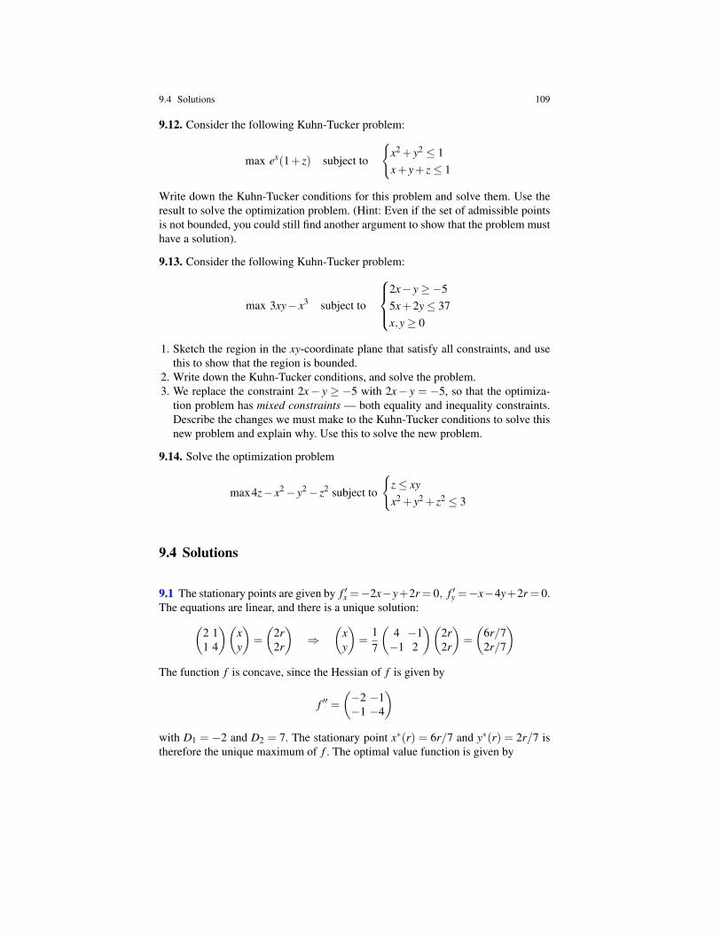
9.4 Solutions 109
9.12. Consider the following Kuhn-Tucker problem:
max ex(1+ z) subject to
{x2 + y2 ≤ 1x+ y+ z≤ 1
Write down the Kuhn-Tucker conditions for this problem and solve them. Use theresult to solve the optimization problem. (Hint: Even if the set of admissible pointsis not bounded, you could still find another argument to show that the problem musthave a solution).
9.13. Consider the following Kuhn-Tucker problem:
max 3xy− x3 subject to
2x− y≥−55x+2y≤ 37x,y≥ 0
1. Sketch the region in the xy-coordinate plane that satisfy all constraints, and usethis to show that the region is bounded.
2. Write down the Kuhn-Tucker conditions, and solve the problem.3. We replace the constraint 2x− y ≥ −5 with 2x− y = −5, so that the optimiza-
tion problem has mixed constraints — both equality and inequality constraints.Describe the changes we must make to the Kuhn-Tucker conditions to solve thisnew problem and explain why. Use this to solve the new problem.
9.14. Solve the optimization problem
max4z− x2− y2− z2 subject to
{z≤ xyx2 + y2 + z2 ≤ 3
9.4 Solutions
9.1 The stationary points are given by f ′x =−2x−y+2r = 0, f ′y =−x−4y+2r = 0.The equations are linear, and there is a unique solution:(
2 11 4
)(xy
)=
(2r2r
)⇒
(xy
)=
17
(4 −1−1 2
)(2r2r
)=
(6r/72r/7
)The function f is concave, since the Hessian of f is given by
f ′′ =(−2 −1−1 −4
)with D1 = −2 and D2 = 7. The stationary point x∗(r) = 6r/7 and y∗(r) = 2r/7 istherefore the unique maximum of f . The optimal value function is given by
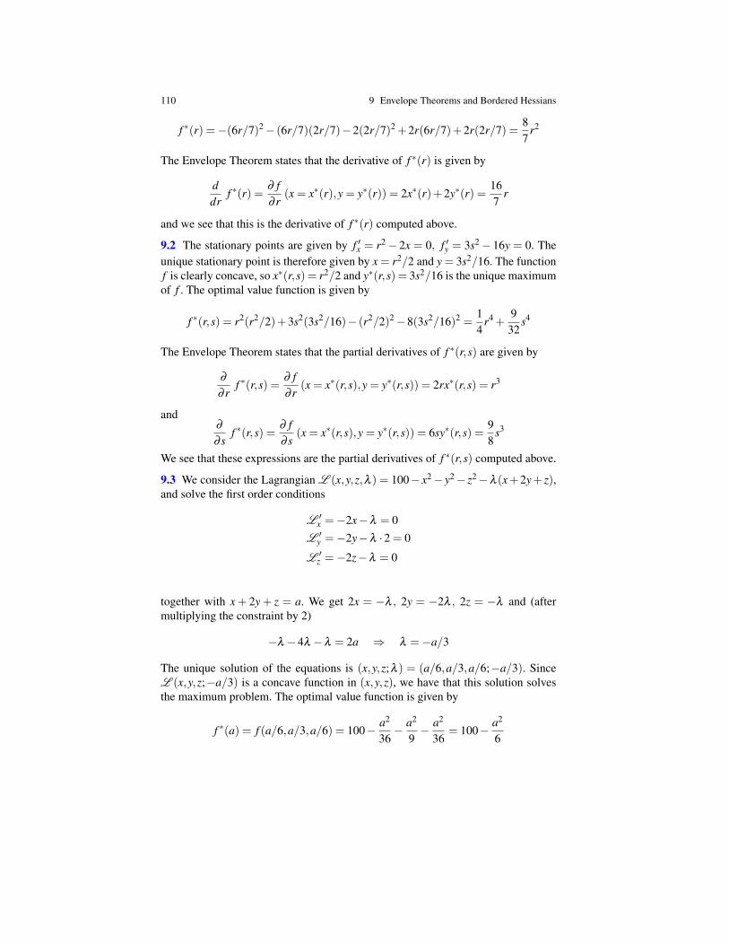
110 9 Envelope Theorems and Bordered Hessians
f ∗(r) =−(6r/7)2− (6r/7)(2r/7)−2(2r/7)2 +2r(6r/7)+2r(2r/7) =87
r2
The Envelope Theorem states that the derivative of f ∗(r) is given by
ddr
f ∗(r) =∂ f∂ r
(x = x∗(r),y = y∗(r)) = 2x∗(r)+2y∗(r) =167
r
and we see that this is the derivative of f ∗(r) computed above.
9.2 The stationary points are given by f ′x = r2− 2x = 0, f ′y = 3s2− 16y = 0. Theunique stationary point is therefore given by x = r2/2 and y = 3s2/16. The functionf is clearly concave, so x∗(r,s) = r2/2 and y∗(r,s) = 3s2/16 is the unique maximumof f . The optimal value function is given by
f ∗(r,s) = r2(r2/2)+3s2(3s2/16)− (r2/2)2−8(3s2/16)2 =14
r4 +9
32s4
The Envelope Theorem states that the partial derivatives of f ∗(r,s) are given by
∂
∂ rf ∗(r,s) =
∂ f∂ r
(x = x∗(r,s),y = y∗(r,s)) = 2rx∗(r,s) = r3
and∂
∂ sf ∗(r,s) =
∂ f∂ s
(x = x∗(r,s),y = y∗(r,s)) = 6sy∗(r,s) =98
s3
We see that these expressions are the partial derivatives of f ∗(r,s) computed above.
9.3 We consider the Lagrangian L (x,y,z,λ ) = 100− x2− y2− z2−λ (x+2y+ z),and solve the first order conditions
L ′x =−2x−λ = 0
L ′y =−2y−λ ·2 = 0
L ′z =−2z−λ = 0
together with x + 2y + z = a. We get 2x = −λ , 2y = −2λ , 2z = −λ and (aftermultiplying the constraint by 2)
−λ −4λ −λ = 2a ⇒ λ =−a/3
The unique solution of the equations is (x,y,z;λ ) = (a/6,a/3,a/6;−a/3). SinceL (x,y,z;−a/3) is a concave function in (x,y,z), we have that this solution solvesthe maximum problem. The optimal value function is given by
f ∗(a) = f (a/6,a/3,a/6) = 100− a2
36− a2
9− a2
36= 100− a2
6
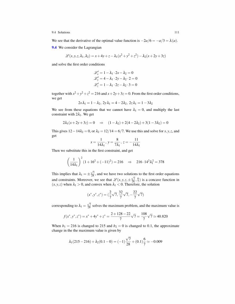
9.4 Solutions 111
We see that the derivative of the optimal value function is −2a/6 =−a/3 = λ (a).
9.4 We consider the Lagrangian
L (x,y,z,λ1,λ2) = x+4y+ z−λ1(x2 + y2 + z2)−λ2(x+2y+3z)
and solve the first order conditions
L ′x = 1−λ1 ·2x−λ2 = 0
L ′y = 4−λ1 ·2y−λ2 ·2 = 0
L ′z = 1−λ1 ·2z−λ2 ·3 = 0
together with x2+y2+z2 = 216 and x+2y+3z = 0. From the first order conditions,we get
2xλ1 = 1−λ2, 2yλ1 = 4−2λ2, 2zλ1 = 1−3λ2
We see from these equations that we cannot have λ1 = 0, and multiply the lastconstraint with 2λ1. We get
2λ1(x+2y+3z) = 0 ⇒ (1−λ2)+2(4−2λ2)+3(1−3λ2) = 0
This gives 12−14λ2 = 0, or λ2 = 12/14 = 6/7. We use this and solve for x,y,z, andget
x =1
14λ1, y =
87λ1
, z =− 1114λ1
Then we substitute this in the first constraint, and get(1
14λ1
)2
(1+162 +(−11)2) = 216 ⇒ 216 ·142λ
21 = 378
This implies that λ1 = ±√
728 , and we have two solutions to the first order equations
and constraints. Moreover, we see that L (x,y,z,±√
728 ,
67 ) is a concave function in
(x,y,z) when λ1 > 0, and convex when λ1 < 0. Therefore, the solution
(x∗,y∗,z∗) = (27
√7,
327
√7,−22
7
√7)
corresponding to λ1 =√
728 solves the maximum problem, and the maximum value is
f (x∗,y∗,z∗) = x∗+4y∗+ z∗ =2+128−22
7
√7 =
1087
√7' 40.820
When b1 = 216 is changed to 215 and b2 = 0 is changed to 0.1, the approximatechange in the the maximum value is given by
λ1(215−216)+λ2(0.1−0) = (−1)
√7
28+(0.1)
67'−0.009
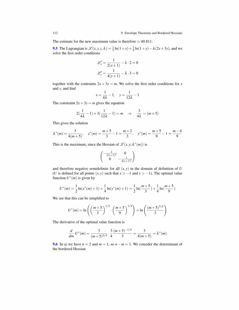
112 9 Envelope Theorems and Bordered Hessians
The estimate for the new maximum value is therefore ' 40.811.
9.5 The Lagrangian is L (x,y,z,λ ) = 12 ln(1+x)+ 1
4 ln(1+y)−λ (2x+3y), and wesolve the first order conditions
L ′x =
12(x+1)
−λ ·2 = 0
L ′y =
14(y+1)
−λ ·3 = 0
together with the contraints 2x+ 3y = m. We solve the first order conditions for xand y, and find
x =1
4λ−1, y =
112λ−1
The constraint 2x+3y = m gives the equation
2(1
4λ−1)+3(
112λ−1) = m ⇒ 3
4λ= (m+5)
This gives the solution
λ∗(m) =
34(m+5)
, x∗(m) =m+5
3−1 =
m+23
, y∗(m) =m+5
9−1 =
m−49
This is the maximum, since the Hessian of L (x,y;λ ∗(m)) is(− 1
2(x+1)2 00 − 1
4(y+1)2
)
and therefore negative semidefinite for all (x,y) in the domain of definition of U(U is defined for all points (x,y) such that x > −1 and y > −1). The optimal valuefunction U∗(m) is given by
U∗(m) =12
ln(x∗(m)+1)+14
ln(y∗(m)+1) =12
ln(m+5
3)+
14
ln(m+5
9)
We see that this can be simplified to
U∗(m) = ln
((m+5
3
)1/2
·(
m+59
)1/4)
= ln
((m+5)3/4
3
)
The derivative of the optimal value function is
ddm
U∗(m) =3
(m+5)3/4 ·34(m+5)−1/4
3=
34(m+5)
= λ∗(m)
9.6 In a) we have n = 2 and m = 1, so n−m = 1. We consider the determinant ofthe bordered Hessian
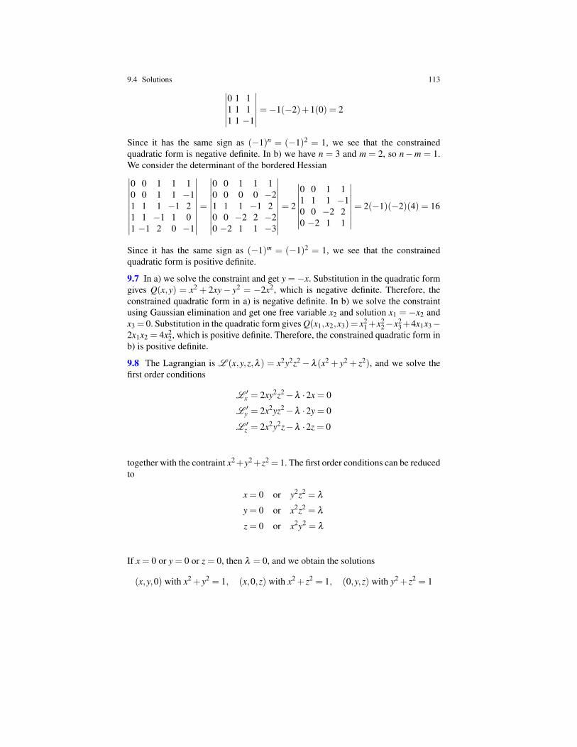
9.4 Solutions 113∣∣∣∣∣∣0 1 11 1 11 1 −1
∣∣∣∣∣∣=−1(−2)+1(0) = 2
Since it has the same sign as (−1)n = (−1)2 = 1, we see that the constrainedquadratic form is negative definite. In b) we have n = 3 and m = 2, so n−m = 1.We consider the determinant of the bordered Hessian∣∣∣∣∣∣∣∣∣∣0 0 1 1 10 0 1 1 −11 1 1 −1 21 1 −1 1 01 −1 2 0 −1
∣∣∣∣∣∣∣∣∣∣=
∣∣∣∣∣∣∣∣∣∣0 0 1 1 10 0 0 0 −21 1 1 −1 20 0 −2 2 −20 −2 1 1 −3
∣∣∣∣∣∣∣∣∣∣= 2
∣∣∣∣∣∣∣∣0 0 1 11 1 1 −10 0 −2 20 −2 1 1
∣∣∣∣∣∣∣∣= 2(−1)(−2)(4) = 16
Since it has the same sign as (−1)m = (−1)2 = 1, we see that the constrainedquadratic form is positive definite.
9.7 In a) we solve the constraint and get y =−x. Substitution in the quadratic formgives Q(x,y) = x2 + 2xy− y2 = −2x2, which is negative definite. Therefore, theconstrained quadratic form in a) is negative definite. In b) we solve the constraintusing Gaussian elimination and get one free variable x2 and solution x1 = −x2 andx3 = 0. Substitution in the quadratic form gives Q(x1,x2,x3)= x2
1+x22−x2
3+4x1x3−2x1x2 = 4x2
2, which is positive definite. Therefore, the constrained quadratic form inb) is positive definite.
9.8 The Lagrangian is L (x,y,z,λ ) = x2y2z2− λ (x2 + y2 + z2), and we solve thefirst order conditions
L ′x = 2xy2z2−λ ·2x = 0
L ′y = 2x2yz2−λ ·2y = 0
L ′z = 2x2y2z−λ ·2z = 0
together with the contraint x2+y2+z2 = 1. The first order conditions can be reducedto
x = 0 or y2z2 = λ
y = 0 or x2z2 = λ
z = 0 or x2y2 = λ
If x = 0 or y = 0 or z = 0, then λ = 0, and we obtain the solutions
(x,y,0) with x2 + y2 = 1, (x,0,z) with x2 + z2 = 1, (0,y,z) with y2 + z2 = 1
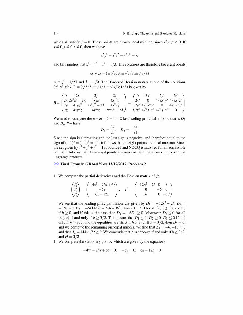
114 9 Envelope Theorems and Bordered Hessians
which all satisfy f = 0. These points are clearly local minima, since x2y2z2 ≥ 0. Ifx 6= 0,y 6= 0,z 6= 0, then we have
x2y2 = x2z2 = y2z2 = λ
and this implies that x2 = y2 = z2 = 1/3. The solutions are therefore the eight points
(x,y,z) = (±√
3/3,±√
3/3,±√
3/3)
with f = 1/27 and λ = 1/9. The Bordered Hessian matrix at one of the solutions(x∗,y∗,z∗;λ ∗) = (
√3/3,±
√3/3,±
√3/3;1/3) is given by
B=
0 2x 2y 2z2x 2y2z2−2λ 4xyz2 4xy2z2y 4xyz2 2x2z2−2λ 4x2yz2z 4xy2z 4x2yz 2x2y2−2λ
=
0 2x∗ 2y∗ 2z∗
2x∗ 0 4/3x∗y∗ 4/3x∗z∗
2y∗ 4/3x∗y∗ 0 4/3y∗z∗
2z∗ 4/3x∗z∗ 4/3y∗z∗ 0
We need to compute the n−m = 3−1 = 2 last leading principal minors, that is D3and D4. We have
D3 =3227
, D4 =−6481
Since the sign is alternating and the last sign is negative, and therefore equal to thesign of (−1)n = (−1)3 =−1, it follows that all eight points are local maxima. Sincethe set given by x2+y2+z2 = 1 is bounded and NDCQ is satisfied for all admissiblepoints, it follows that these eight points are maxima, and therefore solutions to theLagrange problem.
9.9 Final Exam in GRA6035 on 13/12/2012, Problem 2
1. We compute the partial derivatives and the Hessian matrix of f : f ′xf ′yf ′z
=
−4x3−2hx+6z−6y
6x−12z
, f ′′ =
−12x2−2h 0 60 −6 06 0 −12
We see that the leading principal minors are given by D1 = −12x2− 2h, D2 =−6D1 and D3 =−6(144x2 +24h−36). Hence D1 ≤ 0 for all (x,y,z) if and onlyif h ≥ 0, and if this is the case then D2 = −6D1 ≥ 0. Moreover, D3 ≤ 0 for all(x,y,z) if and only if h ≥ 3/2. This means that D1 ≤ 0, D2 ≥ 0, D3 ≤ 0 if andonly if h≥ 3/2, and the equalities are strict if h > 3/2. If h = 3/2, then D3 = 0,and we compute the remaining principal minors. We find that ∆1 =−6,−12≤ 0and that ∆2 = 144x2,72≥ 0. We conclude that f is concave if and only if h≥ 3/2,and H = 3/2.
2. We compute the stationary points, which are given by the equations
−4x3−2hx+6z = 0, −6y = 0, 6x−12z = 0
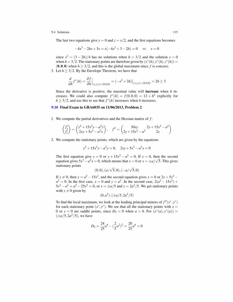
9.4 Solutions 115
The last two equations give y = 0 and z = x/2, and the first equations becomes
−4x3−2hx+3x = x(−4x2 +3−2h) = 0 ⇔ x = 0
since x2 = (3− 2h)/4 has no solutions when h > 3/2 and the solution x = 0when h= 3/2. The stationary points are therefore given by (x∗(h),y∗(h),z∗(h))=(0,0,0) when h≥ 3/2, and this is the global maximum since f is concave.
3. Let h≥ 3/2. By the Envelope Theorem, we have that
ddh
f ∗(h) =∂ f∂h
∣∣∣(x,y,z)=(0,0,0)
= (−x2 +2h)∣∣(x,y,z)=(0,0,0) = 2h≥ 3
Since the derivative is positive, the maximal value will increase when h in-creases. We could also compute f ∗(h) = f (0,0,0) = 12 + h2 explicitly forh≥ 3/2, and use this to see that f ∗(h) increases when h increases.
9.10 Final Exam in GRA6035 on 11/06/2013, Problem 2
1. We compute the partial derivatives and the Hessian matrix of f :(f ′xf ′y
)=
(y2 +15x2y−a2y2xy+5x3−a2x
), f ′′ =
(30xy 2y+15x2−a2
2y+15x2−a2 2x
)2. We compute the stationary points, which are given by the equations
y2 +15x2y−a2y = 0, 2xy+5x3−a2x = 0
The first equation give y = 0 or y+ 15x2 − a2 = 0. If y = 0, then the secondequation gives 5x3−a2x = 0, which means that x = 0 or x =±a/
√5. This gives
stationary points(0,0),(a/
√5,0),(−a/
√5,0)
If y 6= 0, then y = a2− 15x2, and the second equation gives x = 0 or 2y+ 5x2−a2 = 0. In the first case, x = 0 and y = a2. In the second case, 2(a2− 15x2)+5x2−a2 = a2−25x2 = 0, or x =±a/5 and y = 2a2/5. We get stationary pointswith y 6= 0 given by
(0,a2),(±a/5,2a2/5)
To find the local maximum, we look at the leading principal minors of f ′′(x∗,y∗)for each stationary point (x∗,y∗). We see that all the stationary points with x =0 or y = 0 are saddle points, since D2 < 0 when a > 0. For (x∗(a),y∗(a)) =(±a/5,2a2/5), we have
D2 =2425
a4− (25
a2)2 =2025
a4 > 0
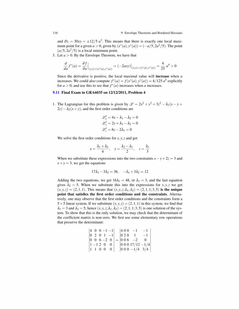
116 9 Envelope Theorems and Bordered Hessians
and D1 = 30xy = ±12/5 a3. This means that there is exactly one local maxi-mum point for a given a > 0, given by (x∗(a),y∗(a)) = (−a/5,2a2/5). The point(a/5,2a2/5) is a local minimum point.
3. Let a > 0. By the Envelope Theorem, we have that
dda
f ∗(a) =∂ f∂a
∣∣∣(x,y)=(x∗(a),y∗(a))
= (−2axy)∣∣(x,y)=(x∗(a),y∗(a)) =
425
a4 > 0
Since the derivative is positive, the local maximal value will increase when aincreases. We could also compute f ∗(a) = f (x∗(a),y∗(a)) = 4/125 a5 explicitlyfor a > 0, and use this to see that f ∗(a) increases when a increases.
9.11 Final Exam in GRA6035 on 12/12/2011, Problem 4
1. The Lagrangian for this problem is given by L = 2x2 + y2 + 3z2− λ1(x− y+2z)−λ2(x+ y), and the first order conditions are
L ′x = 4x−λ1−λ2 = 0
L ′y = 2y+λ1−λ2 = 0
L ′z = 6z−2λ1 = 0
We solve the first order conditions for x,y,z and get
x =λ1 +λ2
4, y =
λ2−λ1
2, z =
λ1
3
When we substitute these expressions into the two constraints x−y+2z = 3 andx+ y = 3, we get the equations
17λ1−3λ2 = 36, −λ1 +3λ2 = 12
Adding the two equations, we get 16λ1 = 48, or λ1 = 3, and the last equationgives λ2 = 5. When we substitute this into the expressions for x,y,z we get(x,y,z) = (2,1,1). This means that (x,y,z;λ1,λ2) = (2,1,1;3,5) is the uniquepoint that satisfies the first order conditions and the constraints. Alterna-tively, one may observe that the first order conditions and the constraints form a5×5 linear system. If we substitute (x,y,z) = (2,1,1) in this system, we find thatλ1 = 3 and λ2 = 5; hence (x,y,z;λ1,λ2) = (2,1,1;3,5) is one solution of the sys-tem. To show that this is the only solution, we may check that the determinant ofthe coefficient matrix is non-zero. We first use some elementary row operationsthat preserve the determinant:∣∣∣∣∣∣∣∣∣∣
4 0 0 −1 −10 2 0 1 −10 0 6 −2 01 −1 2 0 01 1 0 0 0
∣∣∣∣∣∣∣∣∣∣=
∣∣∣∣∣∣∣∣∣∣4 0 0 −1 −10 2 0 1 −10 0 6 −2 00 0 0 17/12 −1/40 0 0 −1/4 3/4
∣∣∣∣∣∣∣∣∣∣
9.4 Solutions 117
Then we see that the determinant is given by 4 ·2 ·6 · (17/4 ·3/4−1/4 ·1/4) =48 6= 0.
2. The bordered Hessian at (x,y,z;λ1,λ2) = (2,1,1;3,5) is the matrix
B =
0 0 1 −1 20 0 1 1 01 1 4 0 0−1 1 0 2 02 0 0 0 6
Since there are n = 3 variables and m = 2 constratints, we have to compute then−m = 1 last principal minors; that is, just the determinant D5 = |B|. We firstuse an elementary row operation to simplify the computation, then develop thedeterminant along the last column:
|B|=
∣∣∣∣∣∣∣∣∣∣0 0 1 −1 20 0 1 1 01 1 4 0 0−1 1 0 2 02 0 0 0 6
∣∣∣∣∣∣∣∣∣∣=
∣∣∣∣∣∣∣∣∣∣0 0 1 −1 20 0 1 1 01 1 4 0 0−1 1 0 2 02 0 −3 3 0
∣∣∣∣∣∣∣∣∣∣= 2
∣∣∣∣∣∣∣∣0 0 1 11 1 4 0−1 1 0 22 0 −3 3
∣∣∣∣∣∣∣∣Then we develop the last determinant along the first row, and get
|B|= 2
∣∣∣∣∣∣∣∣0 0 1 11 1 4 0−1 1 0 22 0 −3 3
∣∣∣∣∣∣∣∣= 2
∣∣∣∣∣∣1 1 0−1 1 22 0 3
∣∣∣∣∣∣−∣∣∣∣∣∣
1 1 4−1 1 02 0 −3
∣∣∣∣∣∣= 2(10+14) = 48
Since |B| = 48 > 0 has the same sign as (−1)m = (−1)2 = 1, we conclude thatthe point (x,y,z) = (2,1,1) is a local minimum for 2x2 + y2 + 3z2 (among theadmissible points). The local minimum value is f (2,1,1) = 8+1+3 = 12.
3. We fix λ1 = 3 and λ2 = 5, and consider the Lagrangian
L (x,y,z) = 2x2 + y2 +3z2−3(x− y+2z)−5(x+ y)
This function is clearly convex, since the Hessian matrix
L ′′ =
4 0 00 2 00 0 6
is positive definite (with eigenvalues 4,2,6). Therefore, the point (x,y,z) =(2,1,1) solves the minimum problem. The Kuhn-Tucker problem can be re-formulated in standard form as
max−(2x2 + y2 +3z2) subject to
{−(x− y+2z) ≤−3−(x+ y) ≤−3
118 9 Envelope Theorems and Bordered Hessians
Therefore, we see that the Lagrangian of the Kuhn-Tucker problem is
−(2x2 + y2 +3z2)+λ1(x− y+2z)+λ2(x+ y) =−L
and the first order conditions of the Kuhn-Tucker problem are the same as in theoriginal problem. Hence (x,y,z;λ1,λ2) = (2,1,1;3,5) is still a solution of thefirst order conditions and the constraints, and λ1,λ2 ≥ 0 also solves the comple-mentary slackness conditions. When we fix λ1 = 3 and λ2 = 5, −L is concavesince L is convex, and this means that (x,y,z) = (2,1,1) also solves the Kuhn-Tucker problem.
9.12 The Kuhn-Tucker problem is in standard form, and its Lagrangian is given by
L = ex(1+ z)−λ1(x2 + y2)−λ2(x+ y+ z)
The Kuhn-Tucker conditions for this problem are the first order conditions
L ′x = ex(1+ z)−λ1(2x)−λ2 = 0
L ′y =−λ1(2y)−λ2 = 0
L ′x = ex−λ2 = 0
the constraints x2 + y2 ≤ 1 and x + y + z ≤ 1, and the complementary slacknessconditions λ1,λ2 ≥ 0 and
λ1(x2 + y2−1) = 0, λ2(x+ y+ z−1) = 0
The last two FOC’s give
λ2 = ex, λ1 =−λ2
2y=− ex
2y
This implies that λ2 > 0 and λ1 6= 0. The CSC therefore give that
x2 + y2 = 1, x+ y+ z = 1, y < 0
and the first FOC that
ex(1+ z)+ ex 2x2y− ex = 0 −→ z+
xy= 0
This means that x = −yz, and therefore that y+ z− yz = 1, or y(1− z) = 1− z.This gives (y− 1)(1− z) = 0, hence y = 1 or z = 1. Since y = 1 gives that λ1 < 0,which is not possible by the CSC, it follows that z = 1. This means that x+ y = 0,or y =−x. Finally, y < 0 from the CSC, so x > 0, and x2 + y2 = 2x2 = 1 means thatx =
√1/2 =
√2/2∼= 0.707. Let us write ω =
√2/2, then we can write the unique
solution of the Kuhn-Tucker conditions FOC+C+CSC as
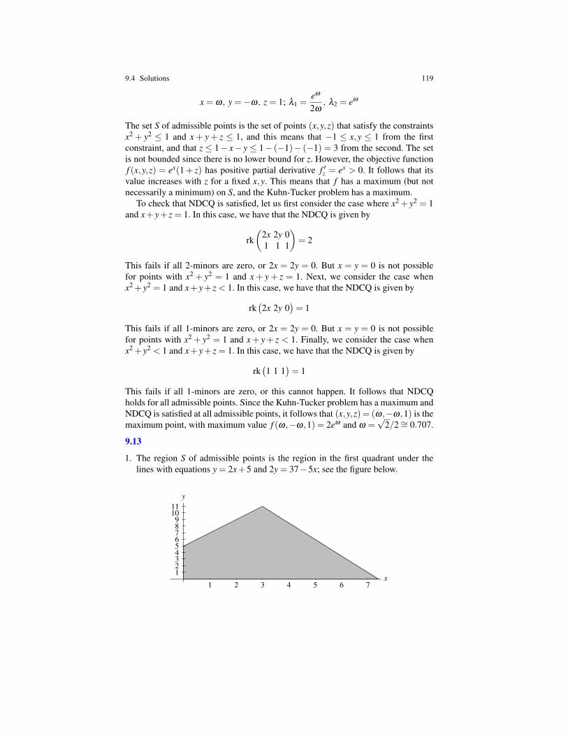
9.4 Solutions 119
x = ω, y =−ω, z = 1; λ1 =eω
2ω, λ2 = eω
The set S of admissible points is the set of points (x,y,z) that satisfy the constraintsx2 + y2 ≤ 1 and x + y + z ≤ 1, and this means that −1 ≤ x,y ≤ 1 from the firstconstraint, and that z ≤ 1− x− y ≤ 1− (−1)− (−1) = 3 from the second. The setis not bounded since there is no lower bound for z. However, the objective functionf (x,y,z) = ex(1+ z) has positive partial derivative f ′z = ex > 0. It follows that itsvalue increases with z for a fixed x,y. This means that f has a maximum (but notnecessarily a minimum) on S, and the Kuhn-Tucker problem has a maximum.
To check that NDCQ is satisfied, let us first consider the case where x2 + y2 = 1and x+ y+ z = 1. In this case, we have that the NDCQ is given by
rk(
2x 2y 01 1 1
)= 2
This fails if all 2-minors are zero, or 2x = 2y = 0. But x = y = 0 is not possiblefor points with x2 + y2 = 1 and x + y+ z = 1. Next, we consider the case whenx2 + y2 = 1 and x+ y+ z < 1. In this case, we have that the NDCQ is given by
rk(2x 2y 0
)= 1
This fails if all 1-minors are zero, or 2x = 2y = 0. But x = y = 0 is not possiblefor points with x2 + y2 = 1 and x+ y+ z < 1. Finally, we consider the case whenx2 + y2 < 1 and x+ y+ z = 1. In this case, we have that the NDCQ is given by
rk(1 1 1
)= 1
This fails if all 1-minors are zero, or this cannot happen. It follows that NDCQholds for all admissible points. Since the Kuhn-Tucker problem has a maximum andNDCQ is satisfied at all admissible points, it follows that (x,y,z) = (ω,−ω,1) is themaximum point, with maximum value f (ω,−ω,1) = 2eω and ω =
√2/2∼= 0.707.
9.13
1. The region S of admissible points is the region in the first quadrant under thelines with equations y = 2x+5 and 2y = 37−5x; see the figure below.
x
y
1 2 3 4 5 6 7
123456789
1011
120 9 Envelope Theorems and Bordered Hessians
Since the first line intersects the y-axis at y = 5, the two lines intersect at x = 3and y = 11, and the second line intersects the x-axis at x = 37/5 = 7.4, it followsthat 0 ≤ x ≤ 7.4 and 0 ≤ y ≤ 11 for all admissible points (x,y), and this meansthat the region of admissible points is bounded.
2. We rewrite the constraints as −2x+ y ≤ 5, 5x+ 2y ≤ 37, −x ≤ 0, and −y ≤ 0,and use this to write the Kuhn-Tucker problem in standard form:
max 3xy− x3 subject to
−2x+ y ≤ 55x+2y ≤ 37−x ≤ 0−y ≤ 0
The Lagrangian for this problem is therefore given by
L = 3xy− x3−λ1(−2x+ y)−λ2(5x+2y)+µ1x+µ2y
where we write µ1,µ2 instead of λ3,λ4. The Kuhn-Tucker conditions for thisproblem are the first order conditions
L ′x = 3y−3x2 +2λ1−5λ2 +µ1 = 0
L ′y = 3x−λ1−2λ2 +µ2 = 0
the constraints −2x+ y ≤ 5, 5x+2y ≤ 37, and x,y ≥ 0, and the complementaryslackness conditions λ1,λ2,µ1,µ2 ≥ 0 and
λ1(−2x+ y−5) = 0, λ2(5x+2y−37) = 0, µ1x = 0, µ2y = 0
We solve FOC+C+CSC to find candidates for maximum, and consider severalcases. The first case is point on the axes. If x = 0, then f (x,y) = 0, and if y = 0,then f (x,y) =−x3 with 0≤ x≤ 7.4. In either case, f (x,y)≤ 0, and this is clearlynot maximum. For example, (x,y) = (1,1) is admissible, and f (1,1) = 2> 0. Wemay therefore assume that x,y> 0, and this means that µ1 = µ2 = 0 by the CSC’s.The second case is the points in the interior of the admissible region (not onany of the boundary lines). This means that all C’s hold by strict inequality, andtherefore also λ1 = λ2 = 0. The FOC’s then give 3y−3x2 = 3x = 0, and the onlysolution is (x,y) = (0,0). This is not an interior point, so there are no candidatepoints in the interior either. We may therefore assume that either −2x+ y = 5 or5x+2y = 37 (or both). We consider three cases:
• The case −2x+ y = 5 and 5x+2y = 37:In this case, x = 3 and y = 11 since this is the intersection between the twolines. This means that −2λ1 + 5λ2 = 6 and λ1 + 2λ2 = 9 by the FOC’s, andthis gives λ1 = 8/3 and λ2 = 11/3. All conditions FOC+C+CSC are satisfied,so this is a candidate point (x,y;λ1,λ2,µ1,µ2) = (3,11;8/3,11/3,0,0) withf = 72.
9.4 Solutions 121
• The case −2x+ y = 5 and 5x+2y < 37:In this case, λ2 = 0 by the CSC’s. This means that 3y− 3x2 + 2λ1 = 0 and3x−λ1 = 0 by the FOC’s. We get λ1 = 3x and therefore 3y−3x2 +6x = 0, ory− x2 + 2x = 0. The constraint −2x+ y = 5 gives (5+ 2x)− x2 + 2x = 0, orx2−4x−5 = 0. The solutions are x = 5 and x =−1, and therefore the points(x,y) = (5,15),(−1,3). The first is not admissible since 5x+2y > 37, and thesecond is not admissible because x < 0. There are no candidate points in thiscase.
• The case −2x+ y < 5 and 5x+2y = 37:In this case, λ1 = 0 by the CSC’s. Hence 3y−3x2−5λ2 = 0 and 3x−2λ2 = 0by the FOC’s. This implies that λ2 = 3x/2 and 3y−3x2−15x/2 = 0. The lastequation can be written 2y− 2x2− 5x = 0, and the constraint 5x+ 2y = 37gives (37−5x)−2x2−5x = 0, or 2x2 +10x−37 = 0. The solutions are
x =−10±
√100−4(2)(−37
4=−10±
√396
4
There are two solutions, one with x < 0 and the other with x ∼= 2.47 < 3.Neither of these are admissible. For the second solution, the reason is thatwhen x < 3, the points on the line 5x+2y = 37 lies over the line −2x+y = 5,and this means −2x+ y > 5. There are no candidate points in this case.
The points (x,y;λ1,λ2,µ1,µ2) = (3,11;8/3,11/3,0,0) is therefore the uniquecandidate point, with f = 72. Since the set of admissible points is bounded, thereis a maximum. Moreover, NDCQ is satisfied at all admissible points: At interiorpoints, there are no conditions to check. At points at the boundary lines (givenby y = 2x+5, 5x+2y = 37, x = 0 and y = 0) that are not corners, there is onlyone binding constraint, and the matrices(
−2 1),(5 2),(−1 0
),(0 −1
)all have rank one. At the corners (0,0), (0,5), (3,11), (7.4,0), there are twobinding constraints, and the matrices(
−1 00 −1
),
(−1 0−2 1
),
(−2 15 2
),
(5 20 −1
)all have rank two. As these are all admissible points, NDCQ holds for all of them,and f = 72 is the maximum value at (x,y) = (3,11).
3. The new problem with mixed constraints can be formulated as
max 3xy− x3 subject to
−2x+ y = 55x+2y ≤ 37−x ≤ 0−y ≤ 0
122 9 Envelope Theorems and Bordered Hessians
To formulate necessary conditions for this mixed problem, we use the same La-grangian as before, given by
L = 3xy− x3−λ1(−2x+ y)−λ2(5x+2y)+µ1x+µ2y
where we write µ1,µ2 instead of λ3,λ4. We must consider the first order condi-tions
L ′x = 3y−3x2 +2λ1−5λ2 +µ1 = 0
L ′y = 3x−λ1−2λ2 +µ2 = 0
the constraints −2x+ y = 5, 5x+2y ≤ 37, and x,y ≥ 0, and the complementaryslackness conditions λ2,µ1,µ2 ≥ 0 and
λ2(5x+2y−37) = 0, µ1x = 0, µ2y = 0
for the three inequality constraints. There is no condition λ1, since it correspondsto an equality constraint. To solve this problem, we can use the computationsabove: We notice that the new set of admissible points consists of the line seg-ment from (0,5) to (3,11). Since this is a subset of the set of old admissiblepoints, shown on the figure above, and the old maximum point (x,y) = (3,11) isstill admissible, it follows that this point is still the maximum point, with maxi-mum value f = 72.
9.14 We rewrite the first constraint as z− xy≤ 0, and write the Lagrangian for thisproblem as
L = 4z− x2− y2− z2−λ1(z− xy)−λ2(x2 + y2 + z2)
The Kuhn-Tucker conditions for this problem are the first order conditions
L ′x =−2x−λ1y−λ2 ·2x = 0
L ′y =−2y−λ1x−λ2 ·2y = 0
L ′x = 4−2z−λ1−λ2 ·2z = 0
the constraints z ≤ xy and x2 + y2 + z2 ≤ 3, and the complementary slackness con-ditions λ1,λ2 ≥ 0 and
z < xy⇒ λ1 = 0, x2 + y2 + z2 < 3⇒ λ2 = 0
Let us find all solutions of the Kuhn-Tucker conditions in the case z = xy and x2 +y2 + z2 = 3. We solve the last of the FOC for λ1 and obtain λ1 = 4− 2z(1+ λ2).Then we substitute this for λ1 in the first two FOC’s and get
−2x− (4−2z(1+λ2))y−2λ2x = 0 ⇒ −2x(1+λ2)+4y−2z(1+λ2)y = 0−2y− (4−2z(1+λ2))x−2λ2y = 0 ⇒ −2y(1+λ2)+4x−2z(1+λ2)x = 0
9.4 Solutions 123
We see that λ2 =−1 gives x = y = 0 and z = xy = 0. But x2+y2+z2 = 0 6= 3 so thisis not possible, and we may assume that λ2 6=−1. Subtraction of the two equationsgives
−2(1+λ2)(x− y)−4(x− y)+2z(1+λ2)(x− y) = 0
This implies that x = y or that (2z− 2)(1+ λ2) = 4. If x = y then z = x2 and thesecond constraint gives 2x2 + x4 = 3. This is a quadratic equation u2 + 2u− 3 = 0in u = x2, with solution x2 = 1 (since x2 = −3 is not possible). Therefore we get(x,y,z) = (1,1,1) or (x,y,z) = (−1,−1,1). In both cases, we see that the FOC’s aresatisfied with λ1 = 2 and λ2 = 0. If x 6= y, then z = 2/(1+λ2)+1 = (3+λ2)/(1+λ2). We substitute this for z in the first FOC, and get
−2x(1+λ2)+4y− (6+2λ2)(1+λ2)y = 0 ⇒ x =λ2−1λ2 +1
y
When we substitute this for x in the second FOC, we get
−2y(1+λ2)+4λ2−1λ2 +1
y− (6+2λ2)λ2−1λ2 +1
y = 0
Multiplication with (1+ λ2) gives y = 0 or −4λ 22 − 4λ2 = 0. If y = 0, then x =
0, and this is not possible since z = xy = 0. If y 6= 0, then we must have λ2 = 0(since (λ2 6=−1), and this implies that z = 3, which is impossible. We conclude thatthe only solutions to the Kuhn-Tucker conditions with both constraints binding are(x,y,z;λ1,λ2) = (1,1,1;2,0),(−1,−1,1;2,0) with f = 1 in both cases. If z < xyand x2 + y2 + z2 = 3, then λ1 = 0 and the first two FOC’s give x = y = 0, so z =−√
3 < xy = 0. But λ2 < 0 from the last FOC, so this is not a solution. If xy = zand x2 + y2 + z2 < 3, then λ2 = 0 and the first two FOC’s imply that x = y and thatλ1 = 2. The third FOC give that z2 = 1. This implies that x = y = z = 1, and thisis not possible since x2 + y2 + z2 < 3. Finally, if z < xy and x2 + y2 + z2 < 3, thenλ1 = λ2 = 0. Then the FOC’s imply that x = y = 0,z = 2 and this is impossiblesince x2 + y2 + z2 < 3. The only solutions occur when both constraints are binding.The set of admissible points is bounded since x2 + y2 + z2 ≤ 3 implies that x,y,z ∈(−√
3,√
3). Therefore the problem has a solution. We consider the NDCQ, and lookat the matrix (
−y −x 12x 2y 2z
)When z = xy and x2 + y2 + z2 = 3, the full matrix has rank two since the first minor−2y2 − 2x2 = 0 if and only if x = y = 0 and this is not possible. If z < xy andx2+y2+z2 = 3, the submatrix consisting of the last row has rank one, since x = y =z = 0 is not possible. If xy = z and x2 +y2 + z2 < 3, then the submatrix consisting ofthe first row clearly has rank one. So there are no admissible points where NDCQis not satisfied, and there must be a maximum at one of the points satisfying theKuhn-Tucker conditions. The conclusion is that (x,y,z) = (1,1,1) and (x,y,z) =(−1,−1,1) are the maximum points, with maximum value f = 1.

Previous: Lecture 9 Contents Next: Lecture 11
Lecture 10First Order Differential Equations
10.1 Main concepts
A differential equation in the function y = y(t) is an equation that contains thederivative y′ = y′(t), or higher order derivatives, such as y′′ = y′′(t) and y′′′ = y′′′(t),or both. A solution is a function y = y(t) that fits in the differential equation. Thereare usually many solutions. The general form of a solution is called the generalsolution.
A first order differential equation involves only y′,y and t since the order of adifferential equation is the highest order of the derivatives involved. In general, afirst order differential equation has the form
y′ = F(t,y)
where F(t,y) is some expression in t and y. The general solution of a first orderdifferential equation will depend on one free variable. An initial value problem con-sists of the differential equation and an initial condition, and has a unique solution,called the particular solution.
Separable differential equations. A first order differential equation is separableif it can be written in the form
y′ = f (t) ·g(y)
for some expressions f (t) in t and g(y) in y. It can be solved using separation of thevariables:
y′ = f (t)g(y) ⇔ 1g(y)
y′ = f (t) ⇔∫ 1
g(y)dy =
∫f (t)dt
After the integrals are computed, one gets a solution in implicit form. To find anexplicit form y = y(t), one must solve for y.
Problems Lecture 10 Solutions
126 10 First Order Differential Equations
Linear differential equations. A first order differential equation is linear if it canbe written in the form
y′+a(t)y = b(t) ⇔ y′ = b(t)−a(t)y
for some expressions a(t),b(t) in t. It can be solved using integrating factor. Theintegrating factor is given by
u = e∫
a(t)dt
and multiplying with u = u(t) in the differential equtation y′+a(t)y = b(t) gives
uy′+a(t)uy = b(t)u ⇔ (uy)′ = b(t)u ⇔ uy =∫
b(t)udt
The solution in explicit form is therefore given by
y =1u·∫
b(t)udt
If a(t) = a and b(t) = b are constants, then the solution is y = b/a+Ce−at .
Exact differential equations. A first order differential equation is exact if it canbe written in the form
p(t,y) · y′+q(t,y) = 0
for some expressions p(t,y),q(t,y) in t and y that satisfies the exactness conditionp′t = q′y. This is the case if and only if there is a function h = h(t,y) such that theequations
h′y = p(t,y) and h′t = q(t,y)
and then the solution of the differential equation is given by h(t,y) =C. To find anexplicit form y = y(t), one must solve for y.
10.2 Problems
10.1. Find the derivative y′ of the following functions:
1. y = 12 t− 3
2 t2 +5t3
2. y = (2t2−1)(t4−1)3. y = (ln t)2−5ln t +64. y = ln(3t)5. y = 5e−3t2+t
6. y = 5t2e−3t
10.2. Compute the following integrals:
1.∫
t3dt2.∫ 1
0 (t3 + t5 + 1
3 )dt
10.2 Problems 127
3.∫ 1
t dt4.∫
tet2dt
5.∫
ln tdt
10.3. Find the general solution, and the particular solution satisfying y(0) = 1 in thefollowing differential equations:
1. y′ = 2t.2. y′ = e2t
3. y′ = (2t +1)et2+t
4. y′ = 2t+1t2+t+1
10.4. We consider the differential equation y′+ y = et . Show that y(t) =Ce−t + 12 et
is a solution of the differential equation for all values of the constant C.
10.5. Show that y = Ct2 is a solution of ty′ = 2y for all choices of the constant C,and find the particular solution satisfying y(1) = 2.
10.6. Solve the differential equation y2y′ = t + 1, and find the integral curve thatgoes through the point (t,y) = (1,1).
10.7. Solve the following differential equations:
1. y′ = t3−12. y′ = tet − t3. eyy′ = t +1
10.8. Solve the following differential equations with initial conditions:
1. ty′ = y(1− t), with (t0,y0) = (1, 1e )
2. (1+ t3)y′ = t2y, with (t0,y0) = (0,2)3. yy′ = t, with (t0,y0) = (
√2,1)
4. e2ty′− y2−2y = 1, with (t0,y0) = (0,0)
10.9. Find the general solution of the differential equation y′+ 12 y = 1
4 . Determinethe equilibrium state of the equation. Is it stable? Draw some typical solutions.
10.10. Find the general solution of the following differential equations:
1. y′+ y = 102. y′−3y = 273. 4y′+5y = 100
10.11. Find the general solution of the following differential equations, and in eachcase, find the particular solution satisfying y(0) = 1:
1. y′−3y = 52. 3y′+2y+16 = 03. y′+2y = t2
128 10 First Order Differential Equations
10.12. Find the general solution of the following differential equations:
1. ty′+2y+ t = 0 (t 6= 0)2. y′− y/t = t (t > 0)
3. y′− tt2−1
y = t (t > 1)
4. y′− 2t
y+2a2
t2 = 0 (t > 0)
10.13. Determine which of the following differential equations are exact, and findthe general solution in those cases where it is exact:
1. (2y+ t)y′+2+ y = 02. y2y′+2t + y = 03. (t5 +6y2)y′+5yt4 +2 = 0
10.14. Solve the differential equation 2t +3y2y′ = 0, first as a separable differentialequation and then as an exact differential equation.
10.15. Final Exam in GRA6035 30/05/2011, 3cSolve the initial value problem (2t + y)− (4y− t)y′ = 0, y(0) = 0.
10.16. Final Exam in GRA6035 10/12/2010, 3cSolve the initial value problem
ty2 y′ =
1y−3t2, y(1) =
13
10.3 Problems in Excel
10.17. We consider the model p′ = k(d− s) for changes in the price p = p(t) givena linear demand function d = a− bp and a linear supply function s = c+ d p. Weassume that a,b,c,d,k > 0 are given positive constants.
1. Solve the model and find the price p(t) as a function of the initial price p0 andthe constants a,b,c,d,k. Use this to determine the equilibrium price
p = limt→∞
p(t)
Solution: linear-model-sol.pdf.2. Realize the model in Excel as shown in this video. You may use this Excel file
as a starting point. Use the numerical values a = 5000, b = 4, c = 1000, d = 6,k = 0.15 and p0 = 200, and a time span from t0 = 0 to T = 10 in N = 100 steps.Solution: linear-model.xlsx.
3. Change the parameters in the Excel model and observe how these changes affectthe price curve. What happens if you increase a (a supply shock)? What happensif you increase k?
10.4 Solutions 129
It is useful to be able to set up an Excel model from scratch. Follow the steps in thisvideo to create the Excel file we used as a starting point above.
10.18. We consider the model y′ = ry(1−y/K) for logistic growth. We assume thatr,K > 0 are given positive constants.
1. Solve the model and express y(t) as a function of r, K, and the initial state y0,and determine the equilibrium states of y. Solution: logistic-model-sol.pdf.
2. Realize the model in Excel as shown in this video. Use the numerical valuesr = 0.5, K = 100, and y0 = 1, and a time span from t0 = 0 to T = 20 in N = 100steps. Solution: logistic-model.xlsx.
3. Change the parameters in the Excel model and observe how these changes affectthe solution curve. What happens if you choose y0 equal to one of the equilibriumstates? What happen if y0 is close to one of these states? What can you say aboutthe stability of the equilibrium states based on this?
10.4 Solutions
10.1
1. y = 12 −3t +15t2
2. y = 4t(t4−1)+(2t2−1)4t3 = 12t5−4t3−4t3. y = 2(ln t) 1
t −5 1t
4. y = 1t
5. y = 5e−3t2+t(−6t +1)6. y = 10te−3t −15t2e−3t
10.2
1.∫
t3dt = 14 t4 +C
2.∫ 1
0 (t3 + t5 + 1
3 )dt = 34
3.∫ 1
t dt = ln |t|+C4. To find the integral
∫tet2
dt we substitute u = t2. This gives dudt = 2t or du
2 = tdt.We get ∫
tet2dt =
∫eu du
2=
12
∫eudu =
12
eu +C =12
et2+C
5. We use integration by parts ∫uv′dt = uv−
∫u′vdt.
We write∫
ln tdt as∫(ln t) ·1dt and let u = ln t and v′ = 1. Thus u′ = 1
t and v = t,and
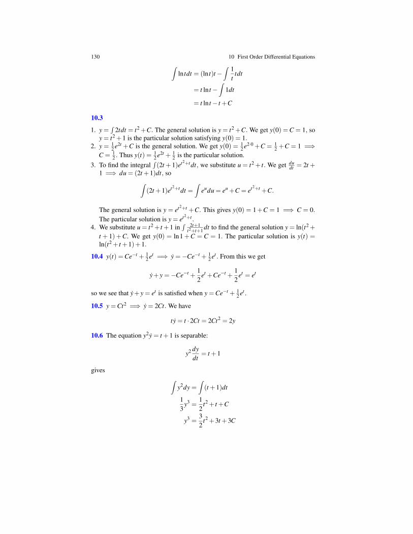
130 10 First Order Differential Equations∫ln tdt = (ln t)t−
∫ 1t
tdt
= t ln t−∫
1dt
= t ln t− t +C
10.3
1. y =∫
2tdt = t2 +C. The general solution is y = t2 +C. We get y(0) =C = 1, soy = t2 +1 is the particular solution satisfying y(0) = 1.
2. y = 12 e2t +C is the general solution. We get y(0) = 1
2 e2·0 +C = 12 +C = 1 =⇒
C = 12 . Thus y(t) = 1
2 e2t + 12 is the particular solution.
3. To find the integral∫(2t +1)et2+tdt, we substitute u = t2 + t. We get du
dt = 2t +1 =⇒ du = (2t +1)dt, so∫
(2t +1)et2+tdt =∫
eudu = eu +C = et2+t +C.
The general solution is y = et2+t +C. This gives y(0) = 1+C = 1 =⇒ C = 0.The particular solution is y = et2+t .
4. We substitute u = t2 + t +1 in∫ 2t+1
t2+t+1 dt to find the general solution y = ln(t2 +
t + 1) +C. We get y(0) = ln1+C = C = 1. The particular solution is y(t) =ln(t2 + t +1)+1.
10.4 y(t) =Ce−t + 12 et =⇒ y =−Ce−t + 1
2 et . From this we get
y+ y =−Ce−t +12
et +Ce−t +12
et = et
so we see that y+ y = et is satisfied when y =Ce−t + 12 et .
10.5 y =Ct2 =⇒ y = 2Ct. We have
ty = t ·2Ct = 2Ct2 = 2y
10.6 The equation y2y = t +1 is separable:
y2 dydt
= t +1
gives ∫y2dy =
∫(t +1)dt
13
y3 =12
t2 + t +C
y3 =32
t2 +3t +3C
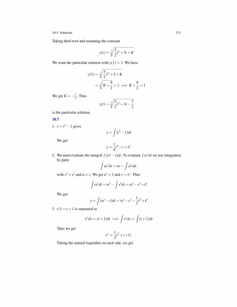
10.4 Solutions 131
Taking third root and renaming the constant
y(t) = 3
√32
t2 +3t +K
We want the particular solution with y(1) = 1. We have
y(1) = 3
√32
12 +3+K
=3
√K +
92= 1 =⇒ K +
92= 1
We get K =− 72 . Thus
y(t) = 3
√32
t2 +3t− 72
is the particular solution.
10.7
1. y = t3−1 gives
y =∫(t3−1)dt
We get
y =14
t4− t +C.
2. We must evaluate the integral∫(tet− t)dt. To evaluate
∫tetdt we use integration
by parts ∫uv′dt = uv−
∫u′vdt.
with v′ = et and u = t. We get u′ = 1 and v = et . Thus∫tetdt = tet −
∫etdt = tet − et +C
We get
y =∫(tet − t)dt = tet − et − 1
2t2 +C
3. eyy = t +1 is separated as
eydy = (t +1)dt =⇒∫
eydy =∫(t +1)dt
Thus we get
ey =12
t2 + t +C.
Taking the natural logarithm on each side, we get
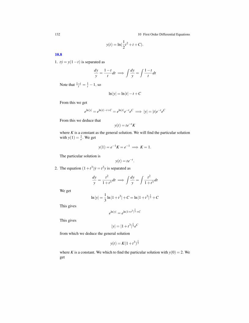
132 10 First Order Differential Equations
y(t) = ln(12
t2 + t +C).
10.8
1. ty = y(1− t) is separated as
dyy
=1− t
tdt =⇒
∫ dyy
=∫ 1− t
tdt
Note that 1−tt = 1
t −1, so
ln |y|= ln |t|− t +C
From this we get
eln |y| = eln |t|−t+C = eln |t|e−teC =⇒ |y|= |t|e−teC
From this we deduce thaty(t) = te−tK
where K is a constant as the general solution. We will find the particular solutionwith y(1) = 1
e . We get
y(1) = e−1K = e−1 =⇒ K = 1.
The particular solution isy(t) = te−t .
2. The equation (1+ t3)y = t2y is separated as
dyy
=t2
1+ t3 dt =⇒∫ dy
y=∫ t2
1+ t3 dt
We get
ln |y|= 13
ln |1+ t3|+C = ln |1+ t3|13 +C
This gives
eln |y| = eln |1+t3|13 +C
This gives|y|= |1+ t3|
13 eC
from which we deduce the general solution
y(t) = K(1+ t3)13
where K is a constant. We which to find the particular solution with y(0) = 2. Weget
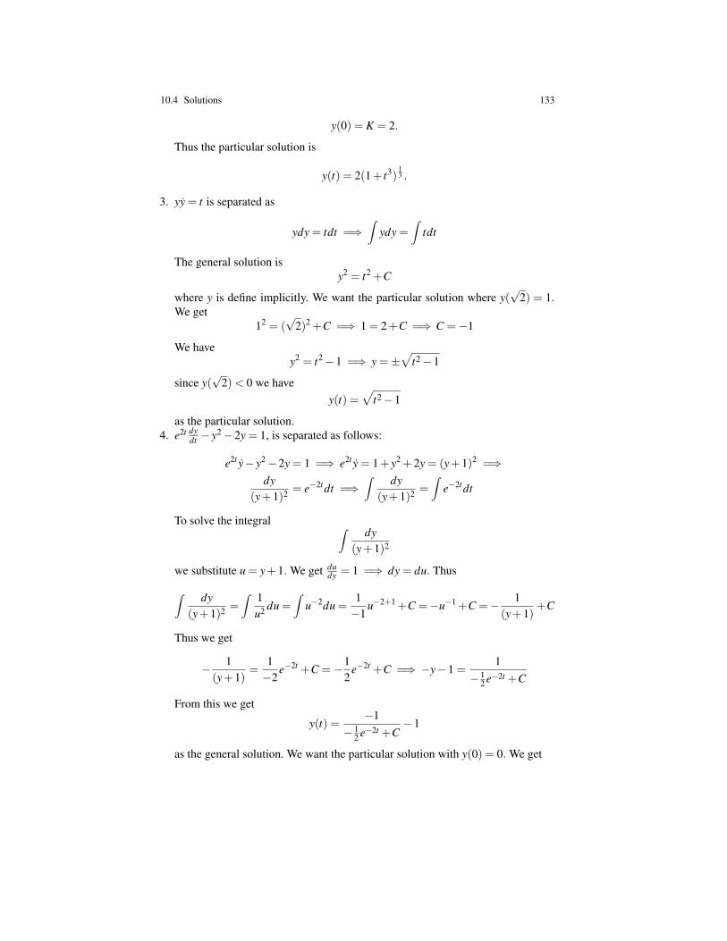
10.4 Solutions 133
y(0) = K = 2.
Thus the particular solution is
y(t) = 2(1+ t3)13 .
3. yy = t is separated as
ydy = tdt =⇒∫
ydy =∫
tdt
The general solution isy2 = t2 +C
where y is define implicitly. We want the particular solution where y(√
2) = 1.We get
12 = (√
2)2 +C =⇒ 1 = 2+C =⇒ C =−1
We havey2 = t2−1 =⇒ y =±
√t2−1
since y(√
2)< 0 we havey(t) =
√t2−1
as the particular solution.4. e2t dy
dt − y2−2y = 1, is separated as follows:
e2t y− y2−2y = 1 =⇒ e2t y = 1+ y2 +2y = (y+1)2 =⇒dy
(y+1)2 = e−2tdt =⇒∫ dy
(y+1)2 =∫
e−2tdt
To solve the integral ∫ dy(y+1)2
we substitute u = y+1. We get dudy = 1 =⇒ dy = du. Thus
∫ dy(y+1)2 =
∫ 1u2 du =
∫u−2du =
1−1
u−2+1+C =−u−1+C =− 1(y+1)
+C
Thus we get
− 1(y+1)
=1−2
e−2t +C =−12
e−2t +C =⇒ −y−1 =1
− 12 e−2t +C
From this we get
y(t) =−1
− 12 e−2t +C
−1
as the general solution. We want the particular solution with y(0) = 0. We get
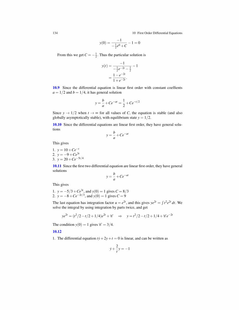
134 10 First Order Differential Equations
y(0) =−1
− 12 e0 +C
−1 = 0
From this we get C =− 12 . Thus the particular solution is
y(t) =−1
− 12 e−2t − 1
2
−1
=1− e−2t
1+ e−2t .
10.9 Since the differential equation is linear first order with constant coeffientsa = 1/2 and b = 1/4, it has general solution
y =ba+Ce−at =
12+Ce−t/2
Since y→ 1/2 when t → ∞ for all values of C, the equation is stable (and alsoglobally asymptotically stable), with equilibrium state y = 1/2.
10.10 Since the differential equations are linear first order, they have general solu-tions
y =ba+Ce−at
This gives
1. y = 10+Ce−t
2. y =−9+Ce3t
3. y = 20+Ce−5t/4
10.11 Since the first two differential equation are linear first order, they have generalsolutions
y =ba+Ce−at
This gives
1. y =−5/3+Ce3t , and y(0) = 1 gives C = 8/32. y =−8+Ce−2t/3, and y(0) = 1 gives C = 9
The last equation has integration factor u = e2t , and this gives ye2t =∫
t2e2t dt. Wesolve the integral by using integration by parts twice, and get
ye2t = (t2/2− t/2+1/4)e2t +C ⇒ y = t2/2− t/2+1/4+C e−2t
The condition y(0) = 1 gives C = 3/4.
10.12
1. The differential equation ty+2y+ t = 0 is linear, and can be written as
y+2t
y =−1
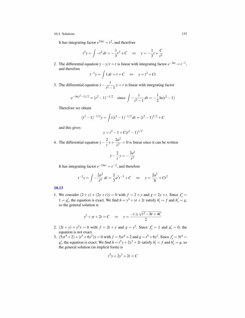
10.4 Solutions 135
It has integrating factor e2ln t = t2, and therefore
t2y =∫−t2 dt =−1
3t3 +C ⇔ y =−1
3t +
Ct2
2. The differential equation y−y/t = t is linear with integrating factor e− ln t = t−1,and therefore
t−1y =∫
1dt = t +C ⇔ y = t2 +Ct
3. The differential equation y− tt2−1
y = t is linear with integrating factor
e− ln(t2−1)/2 = (t2−1)−1/2 since∫− t
t2−1dt =−1
2ln(t2−1)
Therefore we obtain
(t2−1)−1/2y =∫
t(t2−1)−1/2 dt = (t2−1)1/2 +C
and this givesy = t2−1+C(t2−1)1/2
4. The differential equation y− 2t
y+2a2
t2 = 0 is linear since it can be written
y− 2t
y =−2a2
t2
It has integrating factor e−2ln t = t−2, and therefore
t−2y =∫−2a2
t4 dt =23
a2t−3 +C ⇔ y =2a2
3t+Ct2
10.13
1. We consider (2+ y)+ (2y+ t)y = 0 with f = 2+ y and g = 2y+ t. Since f ′y =1 = g′t , the equation is exact. We find h = y2 + yt +2t satisfy h′t = f and h′y = g,so the general solution is
y2 + yt +2t =C ⇒ y =−t±
√t2−8t +4C
2
2. (2t + y) + y2y = 0 with f = 2t + y and g = y2. Since f ′y = 1 and g′t = 0, theequation is not exact.
3. (5yt4+2)+(t5+6y2)y = 0 with f = 5yt4+2 and g = t5+6y2. Since f ′y = 5t4 =
g′t , the equation is exact. We find h = t5y+2y3 +2t satisfy h′t = f and h′y = g, sothe general solution (in implicit form) is
t5y+2y3 +2t =C
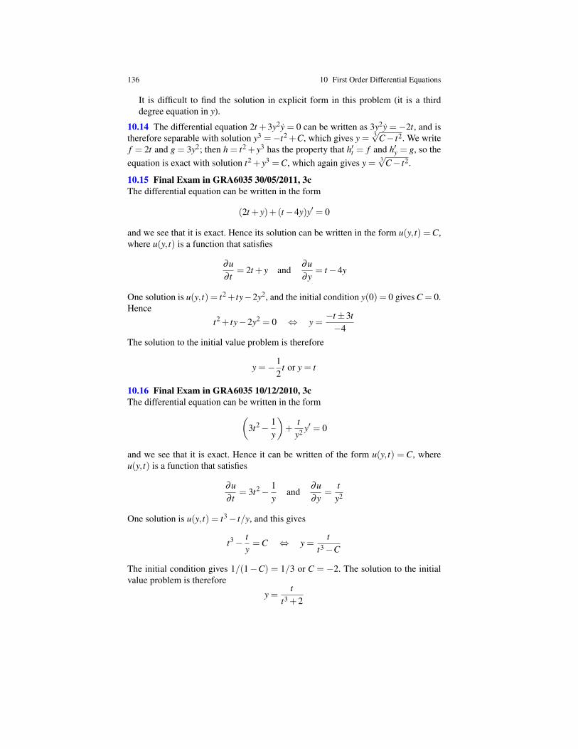
136 10 First Order Differential Equations
It is difficult to find the solution in explicit form in this problem (it is a thirddegree equation in y).
10.14 The differential equation 2t +3y2y = 0 can be written as 3y2y =−2t, and istherefore separable with solution y3 =−t2 +C, which gives y = 3√C− t2. We writef = 2t and g = 3y2; then h = t2 + y3 has the property that h′t = f and h′y = g, so theequation is exact with solution t2 + y3 =C, which again gives y = 3√C− t2.
10.15 Final Exam in GRA6035 30/05/2011, 3cThe differential equation can be written in the form
(2t + y)+(t−4y)y′ = 0
and we see that it is exact. Hence its solution can be written in the form u(y, t) =C,where u(y, t) is a function that satisfies
∂u∂ t
= 2t + y and∂u∂y
= t−4y
One solution is u(y, t) = t2+ ty−2y2, and the initial condition y(0) = 0 gives C = 0.Hence
t2 + ty−2y2 = 0 ⇔ y =−t±3t−4
The solution to the initial value problem is therefore
y =−12
t or y = t
10.16 Final Exam in GRA6035 10/12/2010, 3cThe differential equation can be written in the form(
3t2− 1y
)+
ty2 y′ = 0
and we see that it is exact. Hence it can be written of the form u(y, t) = C, whereu(y, t) is a function that satisfies
∂u∂ t
= 3t2− 1y
and∂u∂y
=ty2
One solution is u(y, t) = t3− t/y, and this gives
t3− ty=C ⇔ y =
tt3−C
The initial condition gives 1/(1−C) = 1/3 or C = −2. The solution to the initialvalue problem is therefore
y =t
t3 +2
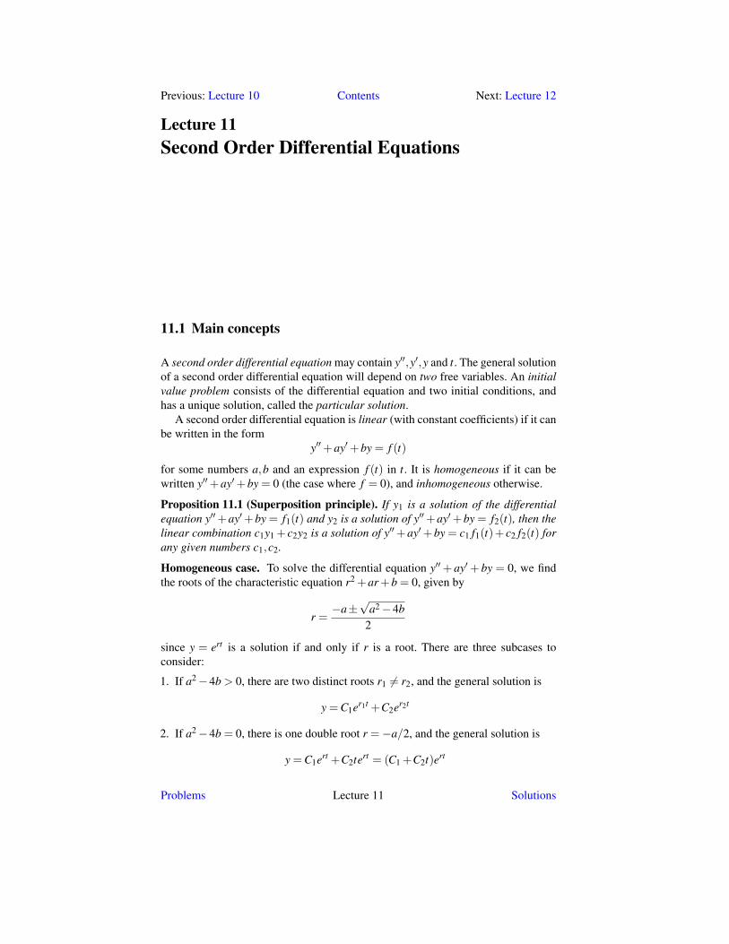
Previous: Lecture 10 Contents Next: Lecture 12
Lecture 11Second Order Differential Equations
11.1 Main concepts
A second order differential equation may contain y′′,y′,y and t. The general solutionof a second order differential equation will depend on two free variables. An initialvalue problem consists of the differential equation and two initial conditions, andhas a unique solution, called the particular solution.
A second order differential equation is linear (with constant coefficients) if it canbe written in the form
y′′+ay′+by = f (t)
for some numbers a,b and an expression f (t) in t. It is homogeneous if it can bewritten y′′+ay′+by = 0 (the case where f = 0), and inhomogeneous otherwise.
Proposition 11.1 (Superposition principle). If y1 is a solution of the differentialequation y′′+ay′+by = f1(t) and y2 is a solution of y′′+ay′+by = f2(t), then thelinear combination c1y1 + c2y2 is a solution of y′′+ay′+by = c1 f1(t)+ c2 f2(t) forany given numbers c1,c2.
Homogeneous case. To solve the differential equation y′′+ ay′+ by = 0, we findthe roots of the characteristic equation r2 +ar+b = 0, given by
r =−a±
√a2−4b
2
since y = ert is a solution if and only if r is a root. There are three subcases toconsider:
1. If a2−4b > 0, there are two distinct roots r1 6= r2, and the general solution is
y =C1er1t +C2er2t
2. If a2−4b = 0, there is one double root r =−a/2, and the general solution is
y =C1ert +C2tert = (C1 +C2t)ert
Problems Lecture 11 Solutions
138 11 Second Order Differential Equations
3. If a2−4b < 0, there are no (real) roots (but two complex roots r = α±β√−1).
The general solution is
y = eαt(C1 cos(β t)+C2 sin(β t))
where α =−a/2 and β =√
4b−a2/2.
Inhomogeneous case. By the superposition principle, the differential equationy′′+ ay′+ by = f (t) has general solution of the form y = yh + yp, where yh is thegeneral solution of the corresponding homogeneous equation y′′+ay′+by = 0, andyp is a particular solution of y′′+ay′+by = f (t).
To find a particular solution yp of y′′ + ay′ + by = f (t), we may considerf (t), f ′(t), f ′′(t) and guess a solution y = yp such that
• The guess for y contains parameter that we may later adjust• The guess for y has the same form as f (t), f ′(t), f ′′(t)
When a guess for y is given, we compute y′,y′′ and insert it in y′′+ay′+by = f (t) tosee if it is a solution for any choices of the parameters. In that case, we have found aparticular solution yp. If the initial guess for y does not work, we may try to multiplyit by t (and thereafter by t2, t3, etc if necessary).
Superposition principle for first order linear differential equations. We mayalso use the superposition principle to solve the first order linear differential equa-tion y′+ ay = b(t), where a is a number and b(t) is an expression in t. This is analternative to the method using integrating factor used in Lecture 10. We obtain thesolution y = yh + yp, and yh =Ce−at since the characteristic equation in this case isr+a = 0 with root r =−a. The general solution is therefore
y =Ce−at + yp
where yp is a particular solution of y′+ay = b(t).
11.2 Problems
11.1. Find the general solution of the following differential equations:
1. y = t2. y = et + t2
11.2. Solve the initial value problem y = t2− t, y(0) = 1, y(0) = 2.
11.3. Solve the initial value problem y = y+ t, y(0) = 1, y(1) = 2.
11.4. Find the general solution of the following differential equations:
1. y−3y = 02. y+4y+8y = 0
11.2 Problems 139
3. 3y+8y = 04. 4y+4y+ y = 05. y+ y−6y = 06. y+3y+2y = 0
11.5. Consider the equation y+ ay+ by = 0 when a2/4− b = 0, so that that thecharacteristic equation has a double root r =−a/2. Let y(t) = u(t)ert and prove thatthis function is a solution if and only if u = 0. Conclude that the general solution isy = (A+Bt)ert .
11.6. Find the general solutions
1. x− x = e−t
2. 3x−30x+75x = 2t +1
11.7. Solve
1. x+2x+ x = t2, x(0) = 0, x(0) = 12. x+4x = 4t +1, x(π
2 ) = 0, x(π
2 ) = 0
11.8. Find the general solutions of the following equations for t > 0. Hint: Insertx = tr into the differential equation and determine for which values of r this is asolution.
1. t2x+5tx+3x = 02. t2x−3tx+3x = t2
11.9. Solve the differential equation x+ 2ax− 3a2x = 100ebt for all values of theconstants a and b.
11.10. Final Exam in GRA6035 30/05/2011, 3bFind the general solution of the differential equation y′′+2y′−35y = 11et −5.
11.11. Final Exam in GRA6035 10/12/2010, 3bFind the general solution of the differential equation y′′+ y′−6y = tet .
11.12. Final Exam in GRA6035 10/12/2007, Problem 3
1. Find the solution of x = (t−2)x2 that satisfies x(0) = 1.2. Find the general solution of the differential equation x−5x+6x = e7t .3. Find the general solution of the differential equation x+2tx = te−t2+t .4. Find the solution of 3x2ex3+3t x+3ex3+3t −2e2t = 0 with x(1) =−1.
11.13. Mock Final Exam in GRA6035 12/2010, Problem 3ab
1. Find the solution of y′ = y(1− y) that satisfies y(0) = 1/2.2. Find the general solution of the differential equation(
ln(t2 +1)−2)
y′ = 2t− 2tyt2 +1
140 11 Second Order Differential Equations
11.14. Final Exam in GRA6035 12/12/2011, Problem 3We consider the differential equation (x+1)tx+(t +1)x = 0 with initial conditionx(1) = 1.
1. Show that the differential equation is separable, and use this to find an implicitexpression for x = x(t). In other words, find an equation of the form
F(x, t) = A
that defines x = x(t) implicitly. It is not necessary to solve this equation for x.2. Show that the differential equation becomes exact after multiplication with ex+t .
Use this to find an implicit expression for x = x(t). In other words, find an equa-tion of the form
G(x, t) = B
that defines x = x(t) implicitly. It is not necessary to solve this equation for x.
11.15. Final Exam in GRA6035 06/02/2012, Problem 3
1. Find the general solution y = y(t) of the differential equation y′′+3y′−10y = 2t.2. Find the general solution y = y(t) of the differential equation 2t +3y2y′ = 2tet2
.3. Find the solution y = y(t) of the differential equation y2+2ty ·y′ = 1 that satisfies
y(1) = 3.
11.16. Final Exam in GRA6035 06/06/2012, Problem 2Find the general solution y = y(t) of the following differential equations:
1. y′′−7y′+12y = t−32. 1−3y2y′ = tet
3. (t/y) · y′+ lny = 1
11.3 Problems in Excel
11.17. We consider the model p′′ = k(d− s) for changes in the price p = p(t) givena linear demand function d = a− bp and a linear supply function s = c+ d p. Weassume that a,b,c,d,k > 0 are given positive constants. Hint: You may use that(sin t)′ = cos t and (cos t)′ =−sin t, and that sin(0) = 0 and cos(0) = 1.
1. Solve the model and find the price p(t) as a function of the initial price p0, p′(0)and the constants a,b,c,d,k. Solution: businesscycle-model-sol.pdf.
2. Realize the model in Excel as shown in this video. You may use this Excel fileas a starting point. Use the numerical values a = 5000, b = 4, c = 1000, d = 6,k = 0.40 and p0 = 100, p′(0) = 200 and a time span from t0 = 0 to T = 10 inN = 100 steps. Solution: businesscycle-model.xlsx.
3. Change the parameters in the Excel model and observe how these changes affectthe price curve. What happens if you increase a (a supply shock)? What happensif you increase k?
11.4 Solutions 141
11.4 Solutions
11.1 We solve the differential equation by direct integration:
1. y = t =⇒ y = 12 t2 +C1 =⇒ y = 1
6 t3 +C1t +C2
2. y = et + t2 =⇒ y = et + 13 t3 +C1 =⇒ y = et + 1
12 t4 +C1t +C2
11.2 We have y = t2− t =⇒ y = 13 t3− 1
2 t2 +C1 =⇒ y = 112 t4− 1
6 t3 +C1t +C2.The initial condition y(0) = 1 gives 1
12 04− 16 03 +C10+C2 =C2 = 1, and y(0) = 2
gives 13 03− 1
2 0+C1 =C1 = 2. The particular solution is therefore
y(t) =1
12t4− 1
6t3 +2t +1
11.3 Substitute u= y. Then y= y+t⇔ u= u+t⇔ u−u= t. The integrating factoris e−t , and we get
ue−t =∫
te−tdt =−e−t − te−t +C1
From this we obtain u = (−e−t − te−t +C1)et = C1et − t − 1 and we integrate tofind y from u = y, and get y =
∫(C1et − t− 1)dt = C1et − t− 1
2 t2 +C2. The initialcondition y(0) = 1 gives C1 +C2 = 1 =⇒ C2 = 1−C1, and the condition y(1) = 2gives C1e−1− 1
2 +C2 =C1e−3/2+1−C1 = 2. This gives C1(e−1) = 5/2, or
C1 =5
2(e−1), C2 = 1− 5
2(e−1)=
2e−72(e−1)
The particular solution is therefore
y(t) =5
2(e−1)· et − t− 1
2t2 +
2e−72(e−1)
11.4
1. The characteristic equation is r2−3r = 0 =⇒ r = 0,3 =⇒ y(t) =C1 +C2e3t .2. Characteristic equation is r2+4r+8 = 0. This has no real solutions. Thus we put
α =− 12 a =− 1
2 4 =−2,β =√
b− 14 a2 =
√8− 1
4 42 = 2. From this the general
solution is y(t) = eαt(Acosβ t +Bsinβ t) = e−2t(Acos2t +Bsin2t).3. 3y+8y= 0⇐⇒ y+ 8
3 y= 0. The characteristic equation is r2+ 83 r = 0 =⇒ r = 0
or r =− 83 . The general solution is y(t) =C1e0t +C2e−
83 t =C1 +C2e−
83 t .
4. 4y+4y+y = 0 has characteristic equation 4r2+4r+1 = 0. There is one solutionr = − 1
2 . The general solution is y(t) = (C1 +C2t)e−12 t .
5. y+ y− 6y = 8 has characteristic equation r2 + r− 6 = 0. It has the solutionsr =−3 and r = 2. The general solution is thus
y(t) =C1e−3t +C2e2t
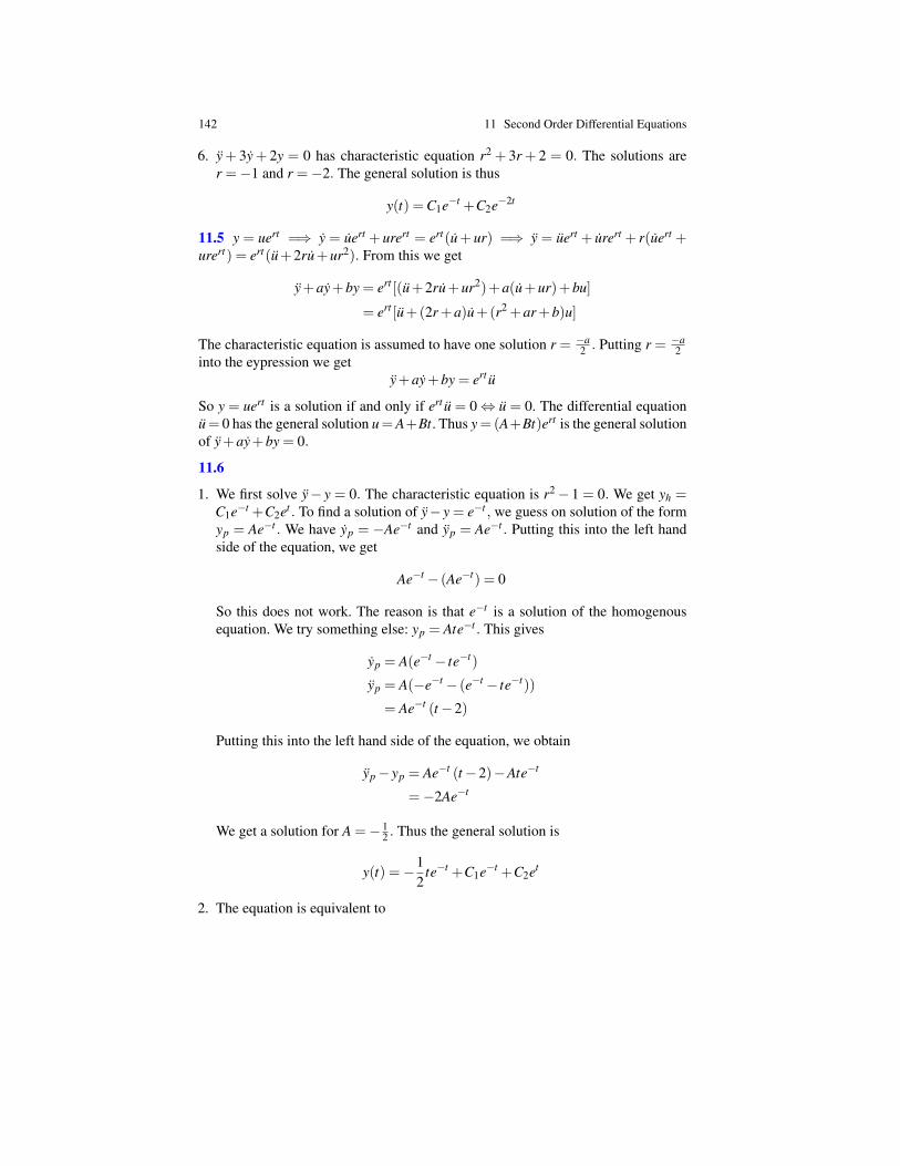
142 11 Second Order Differential Equations
6. y+ 3y+ 2y = 0 has characteristic equation r2 + 3r + 2 = 0. The solutions arer =−1 and r =−2. The general solution is thus
y(t) =C1e−t +C2e−2t
11.5 y = uert =⇒ y = uert + urert = ert(u+ ur) =⇒ y = uert + urert + r(uert +urert) = ert(u+2ru+ur2). From this we get
y+ay+by = ert [(u+2ru+ur2)+a(u+ur)+bu]
= ert [u+(2r+a)u+(r2 +ar+b)u]
The characteristic equation is assumed to have one solution r = −a2 . Putting r = −a
2into the eypression we get
y+ay+by = ert u
So y = uert is a solution if and only if ert u = 0⇔ u = 0. The differential equationu= 0 has the general solution u=A+Bt. Thus y=(A+Bt)ert is the general solutionof y+ay+by = 0.
11.6
1. We first solve y− y = 0. The characteristic equation is r2− 1 = 0. We get yh =C1e−t +C2et . To find a solution of y− y = e−t , we guess on solution of the formyp = Ae−t . We have yp = −Ae−t and yp = Ae−t . Putting this into the left handside of the equation, we get
Ae−t − (Ae−t) = 0
So this does not work. The reason is that e−t is a solution of the homogenousequation. We try something else: yp = Ate−t . This gives
yp = A(e−t − te−t)
yp = A(−e−t − (e−t − te−t))
= Ae−t (t−2)
Putting this into the left hand side of the equation, we obtain
yp− yp = Ae−t (t−2)−Ate−t
=−2Ae−t
We get a solution for A =− 12 . Thus the general solution is
y(t) =−12
te−t +C1e−t +C2et
2. The equation is equivalent to
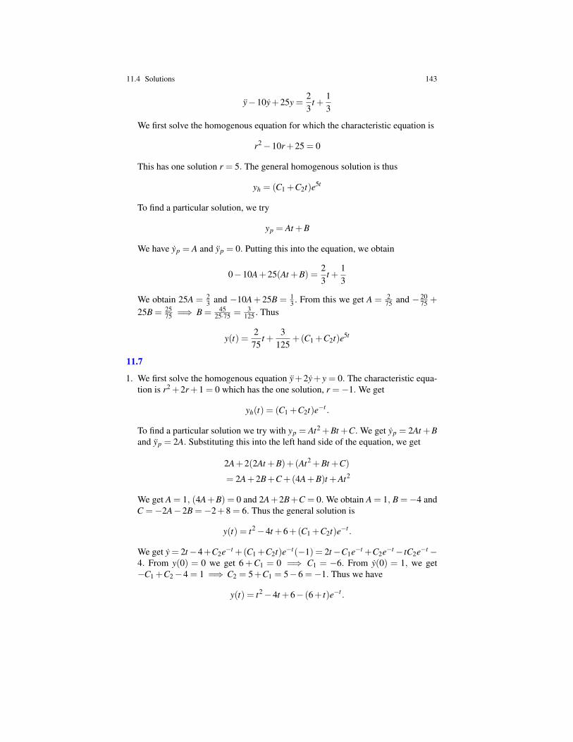
11.4 Solutions 143
y−10y+25y =23
t +13
We first solve the homogenous equation for which the characteristic equation is
r2−10r+25 = 0
This has one solution r = 5. The general homogenous solution is thus
yh = (C1 +C2t)e5t
To find a particular solution, we try
yp = At +B
We have yp = A and yp = 0. Putting this into the equation, we obtain
0−10A+25(At +B) =23
t +13
We obtain 25A = 23 and −10A+ 25B = 1
3 . From this we get A = 275 and − 20
75 +
25B = 2575 =⇒ B = 45
25·75 = 3125 . Thus
y(t) =275
t +3
125+(C1 +C2t)e5t
11.7
1. We first solve the homogenous equation y+2y+ y = 0. The characteristic equa-tion is r2 +2r+1 = 0 which has the one solution, r =−1. We get
yh(t) = (C1 +C2t)e−t .
To find a particular solution we try with yp = At2 +Bt +C. We get yp = 2At +Band yp = 2A. Substituting this into the left hand side of the equation, we get
2A+2(2At +B)+(At2 +Bt +C)
= 2A+2B+C+(4A+B)t +At2
We get A = 1, (4A+B) = 0 and 2A+2B+C = 0. We obtain A = 1, B =−4 andC =−2A−2B =−2+8 = 6. Thus the general solution is
y(t) = t2−4t +6+(C1 +C2t)e−t .
We get y = 2t−4+C2e−t +(C1 +C2t)e−t(−1) = 2t−C1e−t +C2e−t− tC2e−t−4. From y(0) = 0 we get 6 +C1 = 0 =⇒ C1 = −6. From y(0) = 1, we get−C1 +C2−4 = 1 =⇒ C2 = 5+C1 = 5−6 =−1. Thus we have
y(t) = t2−4t +6− (6+ t)e−t .
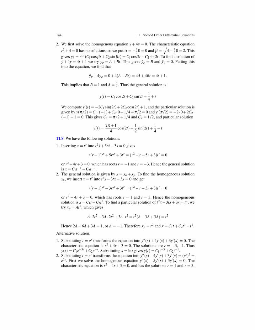
144 11 Second Order Differential Equations
2. We first solve the homogenous equation y+4y = 0. The characteristic equation
r2 +4 = 0 has no solutions, so we put α =− 12 0 = 0 and β =
√4− 1
2 0 = 2. Thisgives yh = eαt(C1 cosβ t +C2 sinβ t) =C1 cos2t +C2 sin2t. To find a solution ofy+ 4y = 4t + 1 we try yp = A+Bt. This gives yp = B and yp = 0. Putting thisinto the equation, we find that
yp +4yp = 0+4(A+Bt) = 4A+4Bt = 4t +1.
This implies that B = 1 and A = 14 . Thus the general solution is
y(t) =C1 cos2t +C2 sin2t +14+ t
We compute y′(t) =−2C1 sin(2t)+2C2 cos(2t)+1, and the particular solution isgiven by y(π/2) =C1 ·(−1)+C2 ·0+1/4+π/2= 0 and y′(π/2) =−2 ·0+2C2 ·(−1)+1 = 0. This gives C1 = π/2+1/4 and C2 = 1/2, and particular solution
y(t) =2π +1
4cos(2t)+
12
sin(2t)+14+ t
11.8 We have the following solutions:
1. Inserting x = tr into t2x+5tx+3x = 0 gives
r(r−1)tr +5rtr +3tr = (r2− r+5r+3)tr = 0
or r2+4r+3= 0, which has roots r =−1 and r =−3. Hence the general solutionis x =C1t−1 +C2t−3.
2. The general solution is given by x = xh + xp. To find the homogeneous solutionxh, we insert x = tr into t2x−3tx+3x = 0 and get
r(r−1)tr−3rtr +3tr = (r2− r−3r+3)tr = 0
or r2− 4r + 3 = 0, which has roots r = 1 and r = 3. Hence the homogeneoussolution is x =C1t +C2t3. To find a particular solution of t2x−3tx+3x = t2, wetry xp = At2, which gives
A ·2t2−3A ·2t2 +3A · t2 = t2(A−3A+3A) = t2
Hence 2A−6A+3A = 1, or A =−1. Therefore xp = t2 and x =C1t +C2t3− t2.
Alternative solution:
1. Substituting t = es transforms the equation into y′′(s)+4y′(s)+3y′(s) = 0. Thecharacteristic equation is r2 + 4r + 3 = 0. The solutions are r = −3,−1. Thusy(s) =C1e−3t +C2e−t . Substituting s = ln t gives y(t) =C1t−3 +C2t−1.
2. Substituting t = es transforms the equation into y′′(s)−4y′(s)+3y′(s) = (es)2 =e2s. First we solve the homogenous equation y′′(s)− 5y′(s) + 3y′(s) = 0. Thecharacteristic equation is r2−4r+3 = 0, and has the solutions r = 1 and r = 3.
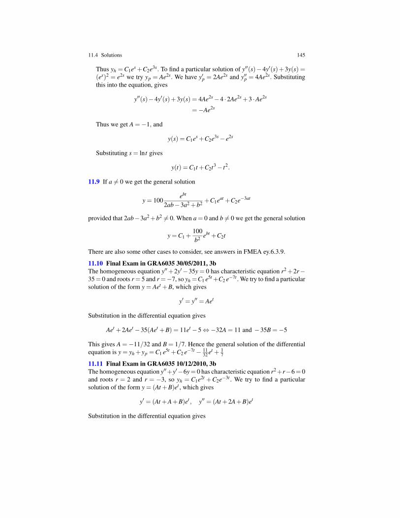
11.4 Solutions 145
Thus yh =C1es +C2e3s. To find a particular solution of y′′(s)−4y′(s)+3y(s) =(es)2 = e2s we try yp = Ae2s. We have y′p = 2Ae2s and y′′p = 4Ae2s. Substitutingthis into the equation, gives
y′′(s)−4y′(s)+3y(s) = 4Ae2s−4 ·2Ae2s +3 ·Ae2s
=−Ae2s
Thus we get A =−1, and
y(s) =C1es +C2e3s− e2s
Substituting s = ln t gives
y(t) =C1t +C2t3− t2.
11.9 If a 6= 0 we get the general solution
y = 100ebt
2ab−3a2 +b2 +C1eat +C2e−3at
provided that 2ab−3a2+b2 6= 0. When a = 0 and b 6= 0 we get the general solution
y =C1 +100b2 ebt +C2t
There are also some other cases to consider, see answers in FMEA ey.6.3.9.
11.10 Final Exam in GRA6035 30/05/2011, 3bThe homogeneous equation y′′+2y′−35y = 0 has characteristic equation r2 +2r−35= 0 and roots r = 5 and r =−7, so yh =C1 e5t +C2 e−7t . We try to find a particularsolution of the form y = Aet +B, which gives
y′ = y′′ = Aet
Substitution in the differential equation gives
Aet +2Aet −35(Aet +B) = 11et −5⇔−32A = 11 and −35B =−5
This gives A =−11/32 and B = 1/7. Hence the general solution of the differentialequation is y = yh + yp =C1 e5t +C2 e−7t − 11
32 et + 17
11.11 Final Exam in GRA6035 10/12/2010, 3bThe homogeneous equation y′′+y′−6y= 0 has characteristic equation r2+r−6= 0and roots r = 2 and r = −3, so yh = C1e2t +C2e−3t . We try to find a particularsolution of the form y = (At +B)et , which gives
y′ = (At +A+B)et , y′′ = (At +2A+B)et
Substitution in the differential equation gives
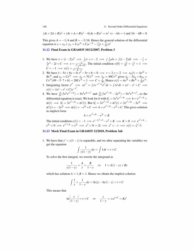
146 11 Second Order Differential Equations
(At +2A+B)et +(At +A+B)et −6(At +B)et = tet ⇔−4A = 1 and 3A−4B = 0
This gives A =−1/4 and B =−3/16. Hence the general solution of the differentialequation is y = yh + yp =C1e2t +C2e−3t − ( 1
4 t + 316 )e
t
11.12 Final Exam in GRA6035 10/12/2007, Problem 3
1. We have x = (t− 2)x2 =⇒ 1x2 x = t− 2 =⇒
∫ 1x2 dx =
∫(t− 2)dt =⇒ − 1
x =12 t2−2t +C =⇒ x = −2
t2−4t+2C . The initial condition x(0) = −22C = −1
C = 1 =⇒C =−1 =⇒ x(t) = −2
t2−4t−2 .2. We have x−5x+6x = 0,r2−5r+6 = 0 =⇒ r = 3,r = 2 =⇒ xh(t) = Ae2t +
Be3t , and xp = Ce7t =⇒ xp = 7Ce7t =⇒ xp = 49Ce7t gives xp− 5xp + 6xp =Ce7t(49−5 ·7+6) = 20Ce7t = 1 =⇒ C = 1
20 . Hence x(t) = Ae2t +Be3t + 120 e7t .
3. Integrating factor et2=⇒ xet2
=∫
te−t2+tet2dt =
∫tetdt = tet − et +C =⇒
x(t) = (tet − et +C)e−t2.
4. We have ∂
∂ t (3x2ex3+3t) = 9x2e3t+x3and ∂
∂x (3ex3+3t − 2e2t) = 9x2e3t+x3, so the
differential equation is exact. We look for h with h′x = 3x2ex3+3t =⇒ h= ex3+3t +
α(t) =⇒ h′t = 3ex3+3t +α ′(t). But h′t = 3ex3+3t +α ′(t) = 3ex3+3t − 2e2t =⇒α ′(t)=−2e2t =⇒ α(t)=−e2t +C =⇒ h= ex3+3t−e2t +C. This gives solutionin implicit form
h = ex3+3t − e2t = K
The initial condition x(1) =−1 =⇒ e(−1)3+3−e2 =K =⇒ K = 0 =⇒ ex3+3t−e2t = 0 =⇒ ex3+3t = e2t =⇒ x3 +3t = 2t =⇒ x3 =−t =⇒ x(t) = 3
√−t.
11.13 Mock Final Exam in GRA6035 12/2010, Problem 3ab
1. We have that y′ = y(1− y) is separable, and we after separating the variables weget the equation ∫ 1
y(1− y)dy =
∫1dt = t +C
To solve the first integral, we rewrite the integrand as
1y(1− y)
=Ay+
B1− y
⇔ 1 = A(1− y)+By
which has solution A = 1,B = 1. Hence we obtain the implicit solution∫ 1y+
11− y
dy = ln |y|− ln |1− y|= t +C
This means that
ln∣∣∣∣ y1− y
∣∣∣∣= t +C ⇔ y1− y
=±et+C = Ket
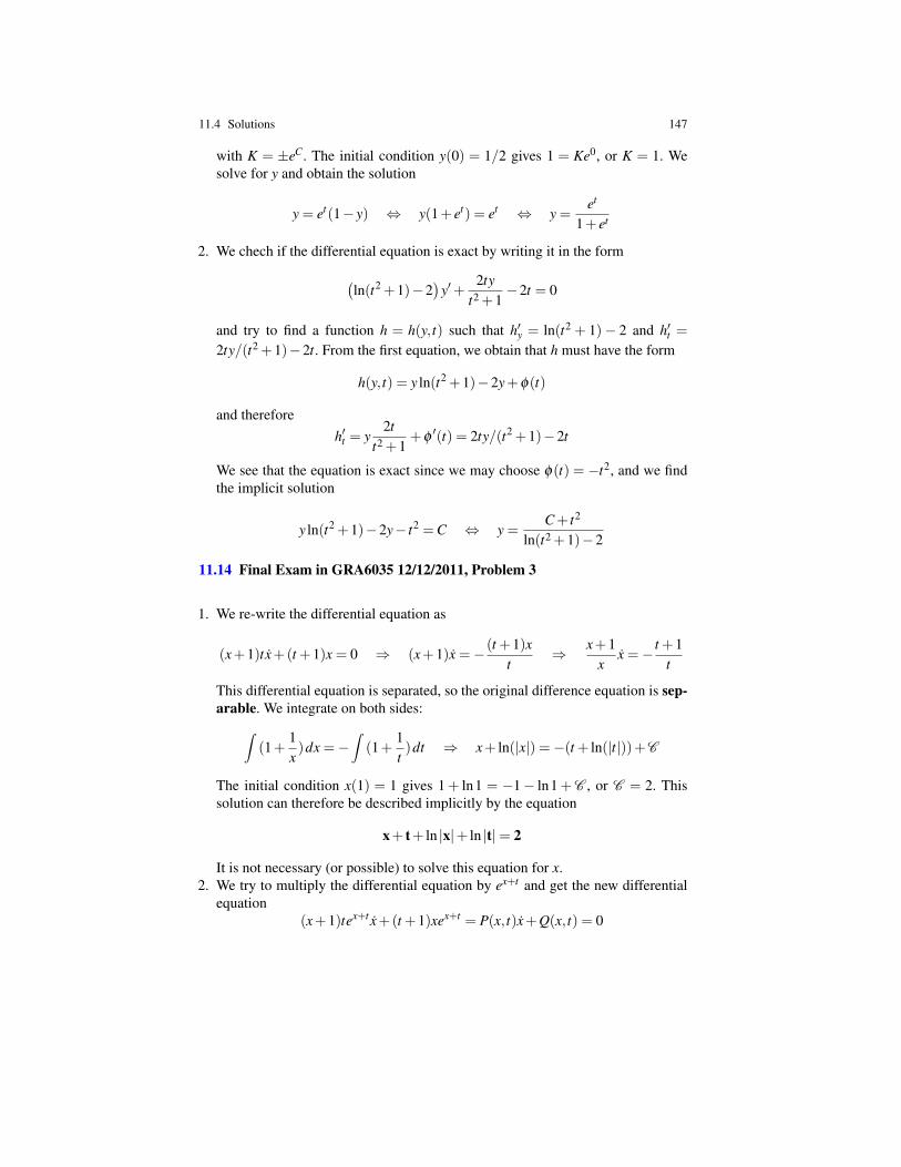
11.4 Solutions 147
with K = ±eC. The initial condition y(0) = 1/2 gives 1 = Ke0, or K = 1. Wesolve for y and obtain the solution
y = et(1− y) ⇔ y(1+ et) = et ⇔ y =et
1+ et
2. We chech if the differential equation is exact by writing it in the form(ln(t2 +1)−2
)y′+
2tyt2 +1
−2t = 0
and try to find a function h = h(y, t) such that h′y = ln(t2 + 1)− 2 and h′t =2ty/(t2 +1)−2t. From the first equation, we obtain that h must have the form
h(y, t) = y ln(t2 +1)−2y+φ(t)
and thereforeh′t = y
2tt2 +1
+φ′(t) = 2ty/(t2 +1)−2t
We see that the equation is exact since we may choose φ(t) = −t2, and we findthe implicit solution
y ln(t2 +1)−2y− t2 =C ⇔ y =C+ t2
ln(t2 +1)−2
11.14 Final Exam in GRA6035 12/12/2011, Problem 3
1. We re-write the differential equation as
(x+1)tx+(t +1)x = 0 ⇒ (x+1)x =− (t +1)xt
⇒ x+1x
x =− t +1t
This differential equation is separated, so the original difference equation is sep-arable. We integrate on both sides:∫
(1+1x)dx =−
∫(1+
1t)dt ⇒ x+ ln(|x|) =−(t + ln(|t|))+C
The initial condition x(1) = 1 gives 1+ ln1 = −1− ln1+C , or C = 2. Thissolution can therefore be described implicitly by the equation
x+ t+ ln |x|+ ln |t|= 2
It is not necessary (or possible) to solve this equation for x.2. We try to multiply the differential equation by ex+t and get the new differential
equation(x+1)tex+t x+(t +1)xex+t = P(x, t)x+Q(x, t) = 0
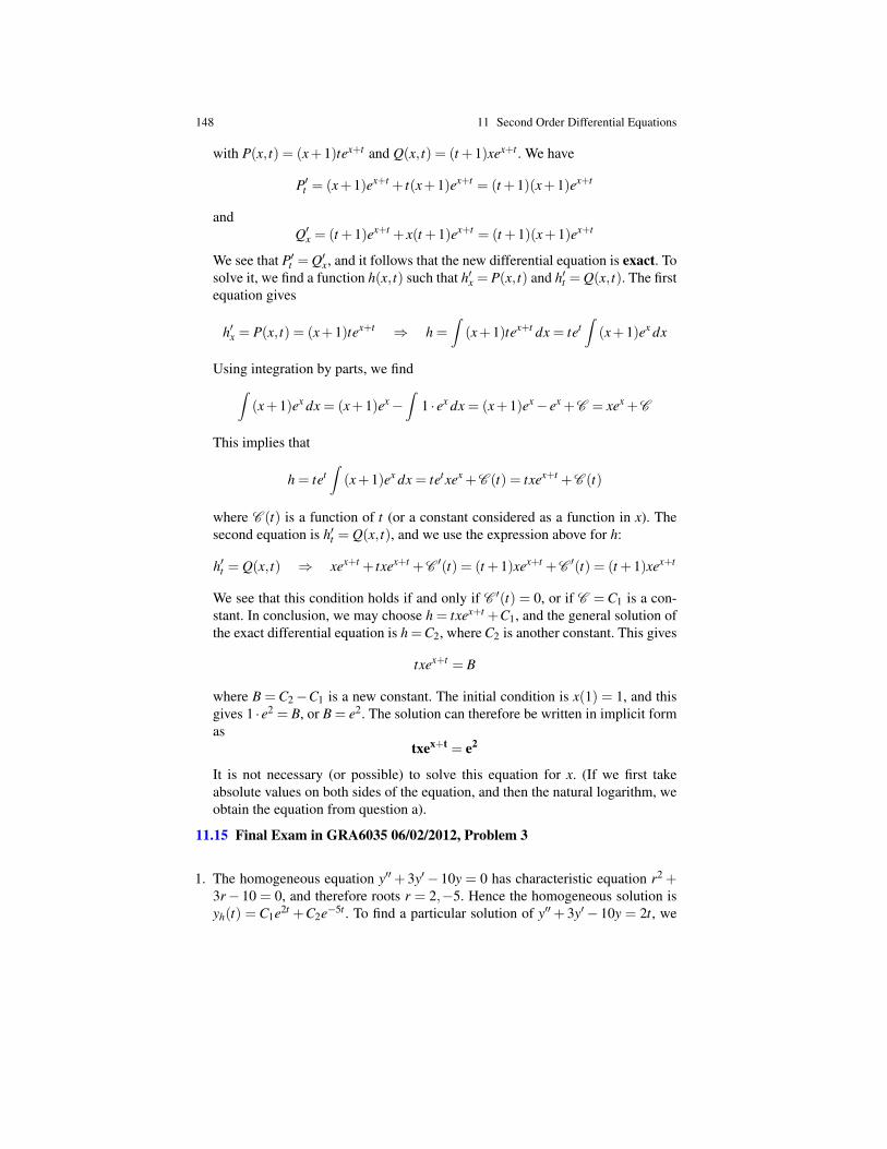
148 11 Second Order Differential Equations
with P(x, t) = (x+1)tex+t and Q(x, t) = (t +1)xex+t . We have
P′t = (x+1)ex+t + t(x+1)ex+t = (t +1)(x+1)ex+t
andQ′x = (t +1)ex+t + x(t +1)ex+t = (t +1)(x+1)ex+t
We see that P′t = Q′x, and it follows that the new differential equation is exact. Tosolve it, we find a function h(x, t) such that h′x = P(x, t) and h′t = Q(x, t). The firstequation gives
h′x = P(x, t) = (x+1)tex+t ⇒ h =∫
(x+1)tex+t dx = tet∫
(x+1)ex dx
Using integration by parts, we find∫(x+1)ex dx = (x+1)ex−
∫1 · ex dx = (x+1)ex− ex +C = xex +C
This implies that
h = tet∫
(x+1)ex dx = tetxex +C (t) = txex+t +C (t)
where C (t) is a function of t (or a constant considered as a function in x). Thesecond equation is h′t = Q(x, t), and we use the expression above for h:
h′t = Q(x, t) ⇒ xex+t + txex+t +C ′(t) = (t +1)xex+t +C ′(t) = (t +1)xex+t
We see that this condition holds if and only if C ′(t) = 0, or if C = C1 is a con-stant. In conclusion, we may choose h = txex+t +C1, and the general solution ofthe exact differential equation is h =C2, where C2 is another constant. This gives
txex+t = B
where B = C2−C1 is a new constant. The initial condition is x(1) = 1, and thisgives 1 ·e2 = B, or B = e2. The solution can therefore be written in implicit formas
txex+t = e2
It is not necessary (or possible) to solve this equation for x. (If we first takeabsolute values on both sides of the equation, and then the natural logarithm, weobtain the equation from question a).
11.15 Final Exam in GRA6035 06/02/2012, Problem 3
1. The homogeneous equation y′′+ 3y′− 10y = 0 has characteristic equation r2 +3r− 10 = 0, and therefore roots r = 2,−5. Hence the homogeneous solution isyh(t) = C1e2t +C2e−5t . To find a particular solution of y′′+ 3y′− 10y = 2t, we
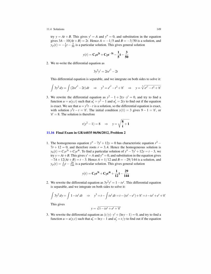
11.4 Solutions 149
try y = At +B. This gives y′ = A and y′′ = 0, and substitution in the equationgives 3A−10(At +B) = 2t. Hence A =−1/5 and B =−3/50 is a solution, andyp(t) =− 1
5 t− 350 is a particular solution. This gives general solution
y(t) = C1e2t +C2e−5t− 15
t− 350
2. We re-write the differential equation as
3y2y′ = 2tet2 −2t
This differential equation is separable, and we integrate on both sides to solve it:∫3y2 dy =
∫(2tet2−2t)dt ⇒ y3 = et2− t2+C ⇒ y =
3√
et2 − t2 +C
3. We rewrite the differential equation as y2 − 1 + 2ty · y′ = 0, and try to find afunction u = u(y, t) such that u′t = y2−1 and u′y = 2ty to find out if the equationis exact. We see that u = y2t− t is a solution, so the differential equation is exact,with solution y2t − t = C . The initial condition y(1) = 3 gives 9− 1 = C , orC = 8. The solution is therefore
t(y2−1) = 8 ⇒ y =
√8t+1
11.16 Final Exam in GRA6035 06/06/2012, Problem 2
1. The homogeneous equation y′′− 7y′+ 12y = 0 has characteristic equation r2−7r + 12 = 0, and therefore roots r = 3,4. Hence the homogeneous solution isyh(t) =C1e3t +C2e4t . To find a particular solution of y′′−7y′+12y = t−3, wetry y=At+B. This gives y′=A and y′′= 0, and substitution in the equation gives−7A+12(At +B) = t−3. Hence A = 1/12 and B =−29/144 is a solution, andyp(t) = 1
12 t− 29144 is a particular solution. This gives general solution
y(t) = C1e3t +C2e4t +112
t− 29144
2. We rewrite the differential equation as 3y2y′ = 1− tet . This differential equationis separable, and we integrate on both sides to solve it:∫
3y2 dy=∫
1−tet dt ⇒ y3 = t−∫
tet dt = t−(tet−et)+C = t−tet +et +C
This givesy = 3√t− tet + et +C
3. We rewrite the differential equation as (t/y) · y′+(lny−1) = 0, and try to find afunction u = u(y, t) such that u′t = lny−1 and u′y = t/y to find out if the equation
150 11 Second Order Differential Equations
is exact. We see that u = t lny− t is a solution, so the differential equation isexact, with solution t lny− t = C or lny−1 = C /t. The solution is therefore
lny =C
t+1 ⇒ y = eC /t+1
Previous: Lecture 11 Contents Next: Lecture II
Lecture 12Difference Equations
12.1 Main concepts
A difference equation is an equation relating the general term yt in the sequence{yt : t = 0,1,2, . . .} with one or more of the term preceeding yt . In general, it hasthe form
yt = F(t,yt−1,yt−2, . . . ,yt−d)
for some positive integer d ≥ 1 called the order of the difference equation. A differ-ence equation is also called a recurrence relation.
Notice that we write yt instead of y(t) for sequences (that is, when y is a functionof t, where t only takes a discrete set of values t = 0,1,2, . . . instead of a continuousset of values). Also notice that any difference equation can be transformed to sucha form that yt is expressed in terms of yt−1, . . . ,yt−d . For instance, the differenceequation yt+1−2yt = t can be tranformed to yt −2yt−1 = t−1 be replacing t witht−1.
A first order difference equation is a difference equation that relates two conse-qutive terms in the sequence. It can be written as
yt = F(t,yt−1)
The general solution will depend on one parameter, and we therefore need one initialcondition to determine a unique solution. A second order difference equation has theform
yt = F(t,yt−1,yt−2)
The general solution will depend on two parameters, and we therefore need twoinitial condition to determine a unique solution.
A first order linear difference equation (with constant coefficients) is a first orderdifference equation that has the form
yt+1 +ayt = ft
Problems Lecture 12 Solutions
152 12 Difference Equations
where a is a given number and ft is an expression in t. It is called homogenous ifft = 0, in which case it has solution
yt+1 +ayt = 0 ⇔ yt =C(−a)t
Otherwise, it is called inhomogeneous, and has solution
yt = yht + yp
t =C(−a)t + ypt
where ypt is a particular solution of yt+1 +ayt = ft .
A second order linear difference equation (with constant coefficients) has theform
yt+2 +ayt+1 +byt = ft
where a,b are given numbers and ft is an expression in t. It is called homogenousif ft = 0. In this case, we consider the characteristic equation r2 + ar+ b = 0, andnotice that r is a root in this equation if and only if rt is a solution of the differenceequation. There are three cases to consider:
1. If a2−4b > 0, there are two distinct roots r1 6= r2, and the general solution is
y =C1rt1 +C2rt
2
2. If a2−4b = 0, there is one double root r =−a/2, and the general solution is
y =C1rt +C2trt = (C1 +C2t)rt
3. If a2− 4b < 0, there are no (real) roots (but two complex roots). The generalsolution is
y = (√
b)t(C1 cos(θ t)+C2 sin(θ t))
where θ is a number such that cos(θ) =− a2√
b.
If ft is non-zero, the difference equation is called inhomogeneous, and it has solution
yt = yht + yp
t
where yht is the general solution of the homogeneous equation yt+2+ayt+1+byt = 0,
and ypt is a particular solution of yt+2 +ayt+1 +byt = ft .
To find a particular solution ypt of a linear difference equation, we may consider
ft , ft+1, ft+2 and guess a solution yt = ypt such that
• The guess for y contains parameter that we may later adjust• The guess for y has the same form as ft , ft+1, ft+2
When a guess for yt is given, we compute yt+1,yt+2 and insert it in the differenceequation to see if it is a solution for any choices of the parameters. In that case, wehave found a particular solution yp. If the initial guess for y does not work, we maytry to multiply it by t (and thereafter by t2, t3, etc if necessary).
12.2 Problems 153
A differential or difference equation is globally asymptotically stable if its gen-eral solution y (with y = y(t) for a differential equation or y = yt for a differenceequation) satisfy
y = limt→∞
y
exists (that is, y it is finite) and is independent of the undetermined coefficients. Theinterpretation of globally asymptotically stable equations is that there is a long termequilibrium y that is independent of the initial conditions.
12.2 Problems
12.1. Find the solution of the difference equation xt+1 = 2xt +4 with x0 = 1.
12.2. Find the solution of the difference equation wt+1 = (1+ r)wt + yt+1− ct+1when r = 0.2, w0 = 1000, yt = 100 and ct = 50.
12.3. Prove by direct substitution that the following sequences in t are solutions ofthe associated difference equations when A,B are constants:
1. xt = A+B ·2t is a solution of xt+2−3xt+1 +2xt = 02. xt = A ·3t +B ·4t is a solution of xt+2−7xt+1 +12xt = 0
12.4. Find the general solution of the difference equation xt+2−2xt+1 + xt = 0.
12.5. Find the general solution of the difference equation 3xt+2−12xt = 4.
12.6. Find the general solution of the following difference equations:
1. xt+2−6xt+1 +8xt = 02. xt+2−8xt+1 +16xt = 03. xt+2 +2xt+1 +3xt = 0
12.7. Find the general solution of the difference equation xt+2 +2xt+1 + xt = 9 ·2t .
12.8. A model for location uses the difference equation
Dt+2−4(ab+1)Dt+1 +4a2b2Dt = 0
where a,b are constants and Dt is the unknown sequence. Find the solution of thisequation assuming that 1+2ab > 0.
12.9. Is the difference equation xt+2− xt+1− xt = 0 globally asymptotically stable?
12.10. Final Exam in GRA6035 10/12/2010, Problem 3aYou borrow an amount K. The interest rate per period is r. The repayment is 500in the first period, and increases with 10 for each subsequent period. Show that theoutstanding balance bt after period t satisfies the difference equation
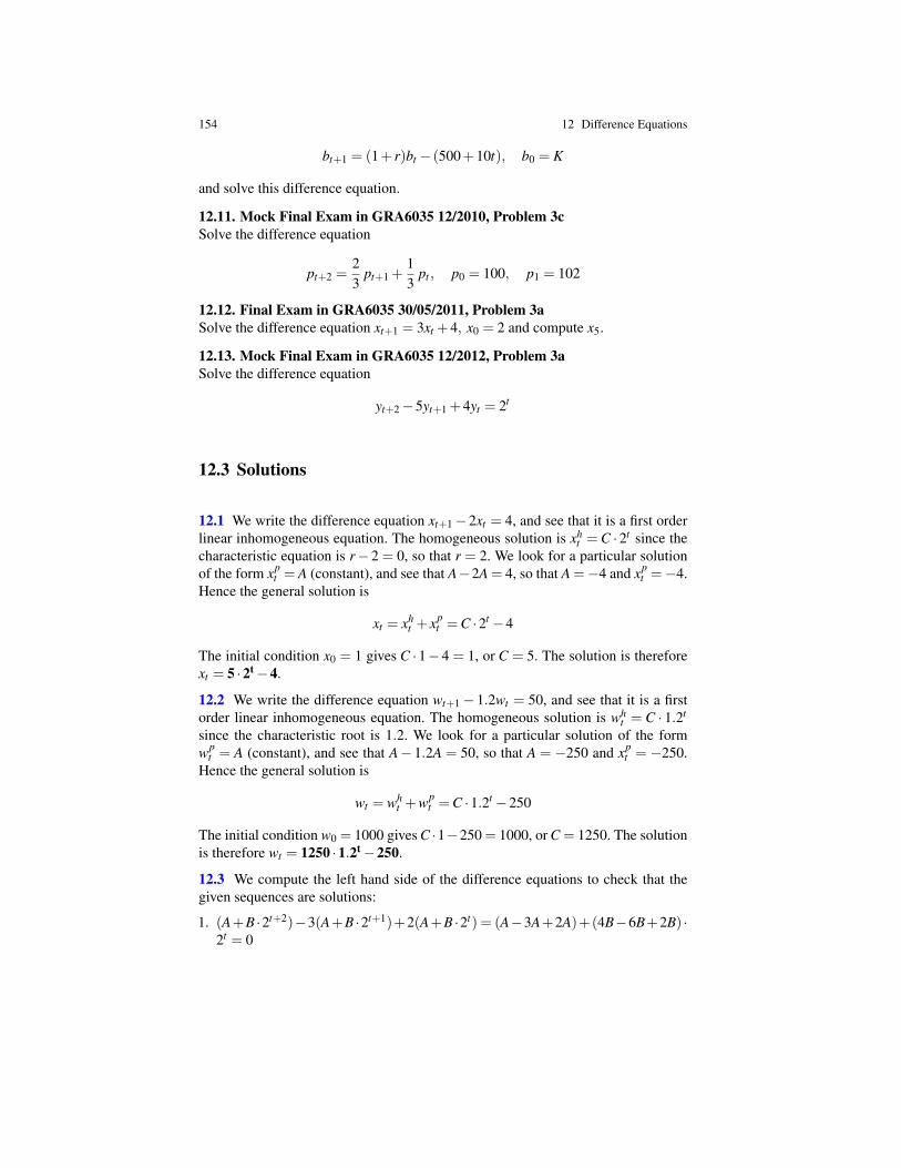
154 12 Difference Equations
bt+1 = (1+ r)bt − (500+10t), b0 = K
and solve this difference equation.
12.11. Mock Final Exam in GRA6035 12/2010, Problem 3cSolve the difference equation
pt+2 =23
pt+1 +13
pt , p0 = 100, p1 = 102
12.12. Final Exam in GRA6035 30/05/2011, Problem 3aSolve the difference equation xt+1 = 3xt +4, x0 = 2 and compute x5.
12.13. Mock Final Exam in GRA6035 12/2012, Problem 3aSolve the difference equation
yt+2−5yt+1 +4yt = 2t
12.3 Solutions
12.1 We write the difference equation xt+1−2xt = 4, and see that it is a first orderlinear inhomogeneous equation. The homogeneous solution is xh
t = C · 2t since thecharacteristic equation is r−2 = 0, so that r = 2. We look for a particular solutionof the form xp
t = A (constant), and see that A−2A = 4, so that A =−4 and xpt =−4.
Hence the general solution is
xt = xht + xp
t =C ·2t −4
The initial condition x0 = 1 gives C ·1−4 = 1, or C = 5. The solution is thereforext = 5 ·2t−4.
12.2 We write the difference equation wt+1− 1.2wt = 50, and see that it is a firstorder linear inhomogeneous equation. The homogeneous solution is wh
t = C · 1.2t
since the characteristic root is 1.2. We look for a particular solution of the formwp
t = A (constant), and see that A− 1.2A = 50, so that A = −250 and xpt = −250.
Hence the general solution is
wt = wht +wp
t =C ·1.2t −250
The initial condition w0 = 1000 gives C ·1−250 = 1000, or C = 1250. The solutionis therefore wt = 1250 ·1.2t−250.
12.3 We compute the left hand side of the difference equations to check that thegiven sequences are solutions:
1. (A+B ·2t+2)−3(A+B ·2t+1)+2(A+B ·2t) = (A−3A+2A)+(4B−6B+2B) ·2t = 0
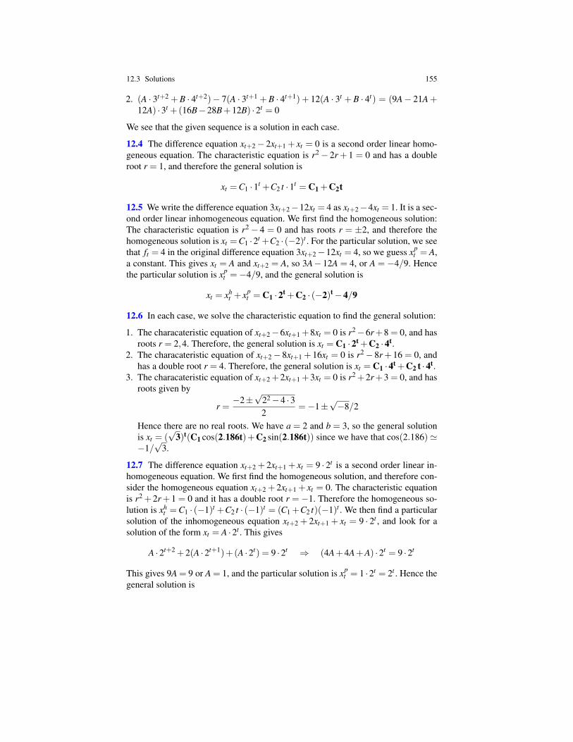
12.3 Solutions 155
2. (A · 3t+2 +B · 4t+2)− 7(A · 3t+1 +B · 4t+1) + 12(A · 3t +B · 4t) = (9A− 21A+12A) ·3t +(16B−28B+12B) ·2t = 0
We see that the given sequence is a solution in each case.
12.4 The difference equation xt+2− 2xt+1 + xt = 0 is a second order linear homo-geneous equation. The characteristic equation is r2− 2r+ 1 = 0 and has a doubleroot r = 1, and therefore the general solution is
xt =C1 ·1t +C2 t ·1t = C1 +C2t
12.5 We write the difference equation 3xt+2−12xt = 4 as xt+2−4xt = 1. It is a sec-ond order linear inhomogeneous equation. We first find the homogeneous solution:The characteristic equation is r2− 4 = 0 and has roots r = ±2, and therefore thehomogeneous solution is xt =C1 ·2t +C2 · (−2)t . For the particular solution, we seethat ft = 4 in the original difference equation 3xt+2−12xt = 4, so we guess xp
t = A,a constant. This gives xt = A and xt+2 = A, so 3A−12A = 4, or A = −4/9. Hencethe particular solution is xp
t =−4/9, and the general solution is
xt = xht + xp
t = C1 ·2t +C2 · (−2)t−4/9
12.6 In each case, we solve the characteristic equation to find the general solution:
1. The characateristic equation of xt+2−6xt+1 +8xt = 0 is r2−6r+8 = 0, and hasroots r = 2,4. Therefore, the general solution is xt = C1 ·2t +C2 ·4t.
2. The characateristic equation of xt+2−8xt+1 +16xt = 0 is r2−8r+16 = 0, andhas a double root r = 4. Therefore, the general solution is xt = C1 ·4t +C2 t ·4t.
3. The characateristic equation of xt+2 +2xt+1 +3xt = 0 is r2 +2r+3 = 0, and hasroots given by
r =−2±
√22−4 ·32
=−1±√−8/2
Hence there are no real roots. We have a = 2 and b = 3, so the general solutionis xt = (
√3)t(C1 cos(2.186t)+C2 sin(2.186t)) since we have that cos(2.186)'
−1/√
3.
12.7 The difference equation xt+2 + 2xt+1 + xt = 9 · 2t is a second order linear in-homogeneous equation. We first find the homogeneous solution, and therefore con-sider the homogeneous equation xt+2 + 2xt+1 + xt = 0. The characteristic equationis r2 +2r+1 = 0 and it has a double root r = −1. Therefore the homogeneous so-lution is xh
t =C1 · (−1)t +C2 t · (−1)t = (C1 +C2 t)(−1)t . We then find a particularsolution of the inhomogeneous equation xt+2 + 2xt+1 + xt = 9 · 2t , and look for asolution of the form xt = A ·2t . This gives
A ·2t+2 +2(A ·2t+1)+(A ·2t) = 9 ·2t ⇒ (4A+4A+A) ·2t = 9 ·2t
This gives 9A = 9 or A = 1, and the particular solution is xpt = 1 ·2t = 2t . Hence the
general solution is
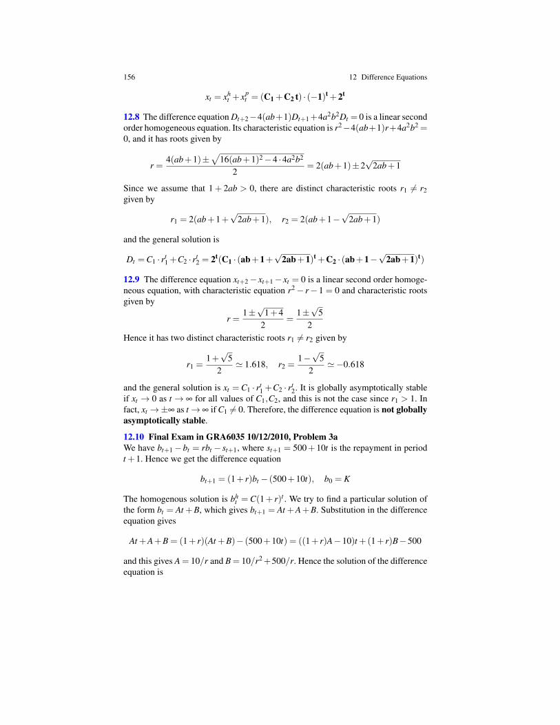
156 12 Difference Equations
xt = xht + xp
t = (C1 +C2 t) · (−1)t +2t
12.8 The difference equation Dt+2−4(ab+1)Dt+1+4a2b2Dt = 0 is a linear secondorder homogeneous equation. Its characteristic equation is r2−4(ab+1)r+4a2b2 =0, and it has roots given by
r =4(ab+1)±
√16(ab+1)2−4 ·4a2b2
2= 2(ab+1)±2
√2ab+1
Since we assume that 1+ 2ab > 0, there are distinct characteristic roots r1 6= r2given by
r1 = 2(ab+1+√
2ab+1), r2 = 2(ab+1−√
2ab+1)
and the general solution is
Dt =C1 · rt1 +C2 · rt
2 = 2t(C1 · (ab+1+√
2ab+1)t +C2 · (ab+1−√
2ab+1)t)
12.9 The difference equation xt+2− xt+1− xt = 0 is a linear second order homoge-neous equation, with characteristic equation r2− r− 1 = 0 and characteristic rootsgiven by
r =1±√
1+42
=1±√
52
Hence it has two distinct characteristic roots r1 6= r2 given by
r1 =1+√
52
' 1.618, r2 =1−√
52
'−0.618
and the general solution is xt = C1 · rt1 +C2 · rt
2. It is globally asymptotically stableif xt → 0 as t → ∞ for all values of C1,C2, and this is not the case since r1 > 1. Infact, xt →±∞ as t→∞ if C1 6= 0. Therefore, the difference equation is not globallyasymptotically stable.
12.10 Final Exam in GRA6035 10/12/2010, Problem 3aWe have bt+1−bt = rbt − st+1, where st+1 = 500+10t is the repayment in periodt +1. Hence we get the difference equation
bt+1 = (1+ r)bt − (500+10t), b0 = K
The homogenous solution is bht = C(1+ r)t . We try to find a particular solution of
the form bt = At +B, which gives bt+1 = At +A+B. Substitution in the differenceequation gives
At +A+B = (1+ r)(At +B)− (500+10t) = ((1+ r)A−10)t +(1+ r)B−500
and this gives A = 10/r and B = 10/r2+500/r. Hence the solution of the differenceequation is
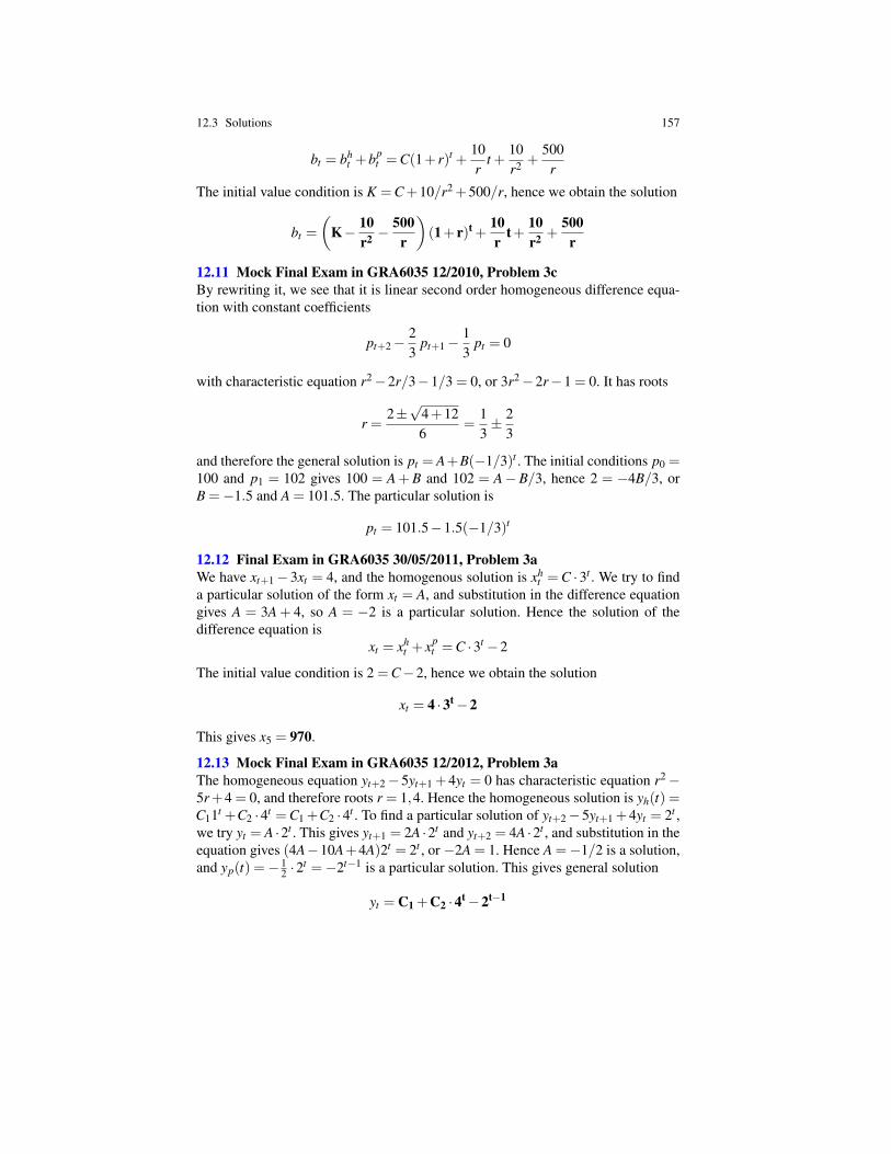
12.3 Solutions 157
bt = bht +bp
t =C(1+ r)t +10r
t +10r2 +
500r
The initial value condition is K =C+10/r2 +500/r, hence we obtain the solution
bt =
(K− 10
r2 −500
r
)(1+ r)t +
10r
t+10r2 +
500r
12.11 Mock Final Exam in GRA6035 12/2010, Problem 3cBy rewriting it, we see that it is linear second order homogeneous difference equa-tion with constant coefficients
pt+2−23
pt+1−13
pt = 0
with characteristic equation r2−2r/3−1/3 = 0, or 3r2−2r−1 = 0. It has roots
r =2±√
4+126
=13± 2
3
and therefore the general solution is pt = A+B(−1/3)t . The initial conditions p0 =100 and p1 = 102 gives 100 = A+B and 102 = A−B/3, hence 2 = −4B/3, orB =−1.5 and A = 101.5. The particular solution is
pt = 101.5−1.5(−1/3)t
12.12 Final Exam in GRA6035 30/05/2011, Problem 3aWe have xt+1−3xt = 4, and the homogenous solution is xh
t = C ·3t . We try to finda particular solution of the form xt = A, and substitution in the difference equationgives A = 3A + 4, so A = −2 is a particular solution. Hence the solution of thedifference equation is
xt = xht + xp
t =C ·3t −2
The initial value condition is 2 =C−2, hence we obtain the solution
xt = 4 ·3t−2
This gives x5 = 970.
12.13 Mock Final Exam in GRA6035 12/2012, Problem 3aThe homogeneous equation yt+2−5yt+1 +4yt = 0 has characteristic equation r2−5r+4 = 0, and therefore roots r = 1,4. Hence the homogeneous solution is yh(t) =C11t +C2 ·4t =C1 +C2 ·4t . To find a particular solution of yt+2−5yt+1 +4yt = 2t ,we try yt = A ·2t . This gives yt+1 = 2A ·2t and yt+2 = 4A ·2t , and substitution in theequation gives (4A−10A+4A)2t = 2t , or −2A = 1. Hence A =−1/2 is a solution,and yp(t) =− 1
2 ·2t =−2t−1 is a particular solution. This gives general solution
yt = C1 +C2 ·4t−2t−1


Part IIExams in GRA6035 Mathematics

Midterm and Final Exams
All exams in GRA 6035 Mathematics (with solutions) since 2009 are available fromthe web page www.dr-eriksen.no/teaching/GRA6035/. Below is a list of links toexams and mock exams (with solutions).
Midterm ExamsMock Midterm Exam in 2010 - Solutions
Midterm Exam on 24/09/2010 - SolutionsMidterm Exam on 24/05/2011 - SolutionsMidterm Exam on 30/09/2011 - SolutionsMidterm Exam on 07/02/2012 - SolutionsMidterm Exam on 19/04/2012 - SolutionsMidterm Exam on 12/10/2012 - SolutionsMidterm Exam on 19/04/2013 - SolutionsMidterm Exam on 11/10/2013 - SolutionsMidterm Exam on 30/04/2014 - SolutionsMidterm Exam on 10/10/2014 - SolutionsMidterm Exam on 27/04/2015 - SolutionsMidterm Exam on 09/10/2015 - SolutionsMidterm Exam on 07/03/2016 - SolutionsMidterm Exam on 07/10/2016 - SolutionsMidterm Exam on 06/01/2017 - SolutionsMidterm Exam on 18/05/2017 - Solutions
Final ExamsMock Final Exam in 2010 - SolutionsMock Final Exam in 2012 - SolutionsMock Final Exam in 2013 - Solutions
Final Exam on 10/12/2010 - SolutionsFinal Exam on 30/05/2011 - SolutionsFinal Exam on 12/12/2011 - SolutionsFinal Exam on 06/02/2012 - SolutionsFinal Exam on 06/06/2012 - SolutionsFinal Exam on 13/12/2012 - SolutionsFinal Exam on 11/06/2013 - SolutionsFinal Exam on 13/12/2013 - SolutionsFinal Exam on 12/05/2014 - SolutionsFinal Exam on 12/12/2014 - SolutionsFinal Exam on 05/05/2015 - SolutionsFinal Exam on 11/12/2015 - SolutionsFinal Exam on 04/03/2016 - SolutionsFinal Exam on 01/12/2016 - SolutionsFinal Exam on 06/01/2017 - SolutionsFinal Exam on 20/06/2017 - Solutions
161