dijkstraw algo
TRANSCRIPT

Dijkstra's algorithm - An Illustrated Explanation
what Dijkstra's Algorithm do?
In a given graph, and starting node, Dijkstra's Algorithm discovers the shortest path from the starting node to all other nodes.
Assumptions: The cost/length of travelling between nodes is known.
The Explanation: Dijkstra's Algorithm
Figure 1: Dijkstra - Initial Position
Figure 1 displays the graph: nodes are black circles labelled a-f, a path is a black line connecting two nodes, each path has an associated length beside it (the numbers). The lengths are not to scale.
Node 'a' is our starting node, we want to find the shortest path to all other nodes in the graph. To do this, we generate a table. This table has the distance to all the nodes in the graph, from the perspective of the starting node 'a'.
Table 1: Initial Entries for distances to nodes from Node 'a'

NodeDistance to Node from Node 'a'
B INFINTE
C INFINTE
D INFINTE
E INFINTE
F INFINTE
G INFINTE
H INFINTE
I INFINTE
As can be seen from Table 1, the initial entries for the distances are all set to infinity (or some notional maximum value). This ensures that any path found will be shorter than the initial value stored in the table.
The node 'a' is the starting node, as such we examine all the possible paths away from this node first. The options are as follows:
Table 2: Distance to nodes (from 'a') accesible from node 'a'
Node Distance to Node from Node 'a'
B 7
C 4
D 5
These values are used to update the graph table, Table 1, which becomes:
Table 3: Entries for distances to nodes from Node 'a'
Node Distance to Node from Node 'a'
B 7
C 4
D 5

E INFINTE
F INFINTE
G INFINTE
H INFINTE
I INFINTE
Figure 2: Dijkstra's algorithm
Figure 2 shows the routes marked in red. We know we have three paths from node 'a'. However, these paths are not yet guaranteed to be the shortest path. To be sure we have the shortest path, we have to keep going.
The next move in the algorithm is to move to the nearest node from node 'a'. In this case that is node 'c'.

Figure 3: Dijkstra's Algorithm
At node 'c' we have paths available to nodes 'b' and 'h'. When calculating the distances we have to calculate the distances from node 'a'. In this case that means the following:
Table 4: Distance to nodes (from 'a') accesible from node 'a'
Node Distance to Node from Node 'a'
B 6
H 13
These values are then compared to the values stored in the Table 3. It can be seen that both of these values are less than the current values stored in the table, as such table 3 becomes:
Table 5: Entries for distances to nodes from Node 'a'
Node Distance to Node from Node 'a'
B 6
C 4
D 5

E INFINTE
F INFINTE
G INFINTE
H 13
I INFINTE
This step has illustrated one of the advantages of dijkstra's algorithm: the route to node 'b' is not the most direct route, but it is the shortest route; Dijkstra's Algorithm can find the shortest route, even when that route is not the most direct route.
Figure 4: Dijkstra's Algorithm
Again, all paths accesible from node 'c' have been checked, and the table of paths has been updated. Node 'c' is marked as visited.
IMPORTANT:
1. A Visited node is never re-visited. 2. Once a node has been marked visited, the path to that node is known
to be the shortest route from the initial node.
In that case, we should add another column to our table:

Table 6: Entries for distances to nodes from Node 'a'
NodeDistance to Node from Node 'a'
Visited
b 6 NO
c 4 YES
d 5 NO
e INFINTE NO
f INFINTE NO
g INFINTE NO
h 13 NO
i INFINTE NO
As these value are being updated, the route that accompanies these distances also needs to be stored.
Once again, the table of paths is consulted, and the shortest path to a node that has not been visited is found. This node becomes the next current node. In this case, that is node 'd'.
Figure 5: Dijkstra's Algorithm

From node 'd', the following paths are available:
Table 7: Distance to nodes (from 'a') accesible from node 'a'
Node Distance to Node from Node 'a'
f 14
The table of all paths is updated to reflect that, and the node 'd' is marked as visited, this locks in the shortest path to node 'd' also:
Table 8: Entries for distances to nodes from Node 'a'
NodeDistance to Node from Node 'a'
Visited
b 6 NO
c 4 YES
d 5 YES
e INFINTE NO
f 14 NO
g INFINTE NO
h 13 NO
i INFINTE NO
It can be seen from table 8 above, that the next nearest node to node 'a' is node 'b'. All paths from node 'b' are examined next. In this instance, we have a path to a node that is marked as visited: node 'c', we already know that the path to node 'c' is as short as it can get (the node being marked as visited is the marker for this).
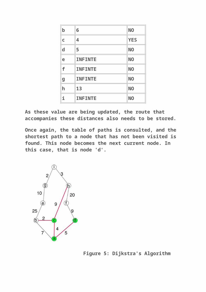
Figure 6: Dijkstra's Algorithm
As figure 6 shows, we check the path the only other node accesible from node 'b': node 'e'. This updates our paht table as follows:
Table 9: Entries for distances to nodes from Node 'a'
NodeDistance to Node from Node 'a'
Visited
b 6 YES
c 4 YES
d 5 YES
e 31 NO
f 14 NO
g INFINTE NO
h 13 NO
i INFINTE NO
Table 9 again tells us that the next node for us to visit is node 'h'.

Figure 7: Dijkstra's Algorithm
We add up the paths, and mark the nodes as visited...
Figure 8: Dijkstra's Algorithm
We keep on doing this....

Figure 9: Dijkstra's Algorithm
Until all the nodes have been visited!
Every step in this process can be viewed as under: Dijkstra's Algorithm - Step-by-Step
Dijkstra's algorithm

Dijkstra 02
Dijkstra 03

Dijkstra 04
Dijkstra 05
Dijkstra 06

Dijkstra 07
Dijkstra 08
Dijkstra 09

Dijkstra 10
Dijkstra 11

Dijkstra's algorithm
Dijkstra 14

Dijkstra 15
Dijkstra 16
Dijkstra 17

Dijkstra 18
Dijkstra 19
Dijkstra 20