diploma thesis - speed · bucharest 2018 university “politehnica” of bucharest faculty of...

Bucharest 2018

UNIVERSITY “POLITEHNICA” OF BUCHAREST

FACULTY OF ELECTRONICS, TELECOMMUNICATION AND

INFORMATION TECHNOLOGY

Speaker Recognition on Embedded System (on NAO Robot)

Diploma Thesis

submitted in partial fulfillment of the requirements for the Degree of

Engineer in the domain Electronics and Telecommunications, study

program Technology and Telecommunication Systems

Thesis Advisor Student

Prof. Ph. D. Corneliu BURILEANU Rebeca-Graţiela Predescu

TABLE OF CONTENTS

Table of Contents.................................................................................................................................7

List of Figures......................................................................................................................................9

List of Tables......................................................................................................................................11

List of Acronyms................................................................................................................................13

CHAPTER 1 Introduction..................................................................................................................15

1.1 Thesis Motivation.............................................................................................................15

1.2 Main Objective.................................................................................................................15

1.3 Specific Objectives..........................................................................................................16

CHAPTER 2 Humanoid Robots.........................................................................................................19

2.1 General Aspects................................................................................................................19

2.2 Applications of Humanoid Robots...................................................................................19

2.3 NAO.................................................................................................................................20

2.3.1 General Features................................................................................................20

2.3.1 Resources...........................................................................................................21

CHAPTER 3 Wiener Filtering...........................................................................................................29

3.1 General Aspects................................................................................................................29

3.2 Random Signals and Spectral Densities...........................................................................29

3.3 Linear Time-Invariant Systems........................................................................................30

3.4 Wiener Filter’s Coefficients.............................................................................................31

3.5 Wiener Filter Used in Noise Reduction............................................................................34

CHAPTER 4 GMM-UBM.................................................................................................................37

4.1 Markov Chains.................................................................................................................37

4.2 The Hidden Markov Model..............................................................................................39

4.3 HMM Training: The Baum-Welch Algorithm.................................................................41

4.4 HMM Applied to Speech..................................................................................................43

4.5 MFCC Vectors..................................................................................................................45

4.5.1 Pre-emphasis......................................................................................................47

4.5.2 Windowing........................................................................................................47

4.5.3 Discrete Fourier Transform...............................................................................49

4.5.4 Mel Filter Bank and Log...................................................................................50

4.5.5 The Inverse Discrete Fourier Transform...........................................................50

4.5.6 Deltas and Energy..............................................................................................51

4.6 Gaussian Mixture Model..................................................................................................52

4.6.1 Univariate Gaussians.........................................................................................52

4.6.2 Multivariate Gaussians......................................................................................54

4.6.2 Gaussian Mixture Model-Motivation................................................................56

4.6.4 Maximum Likelihood Parameter Estimation....................................................58

4.7 Universal Background Model...........................................................................................60

4.7.1 Adaptation of Speaker Model............................................................................60

4.7.2 Log-Likelihood Ratio Computation..................................................................62

CHAPTER 5 Testing the Method.......................................................................................................65

5.1 Database................................................................................................................................65

5.2 Experimental Setup...............................................................................................................65

5.3 Results...................................................................................................................................66

CHAPTER 6 Conclusion....................................................................................................................81

REFERENCES...................................................................................................................................83

LIST OF FIGURES

Figure 1.1 Implementation Steps..................................................................................................16

Figure 2.3.1 NAO Robot..............................................................................................................20

Figure 2.3.2.1 Microphones’ Location.........................................................................................21

Figure 2.3.2.2 Cameras Used for Object Identification................................................................22

Figure 2.3.2.3 Camera Used to Detect Obstacles.........................................................................22

Figure 2.3.2.4 LED Positions.......................................................................................................23

Figure 2.3.2.5 FSR Sensors..........................................................................................................24

Figure 2.3.2.6 Inertial Unit...........................................................................................................24

Figure 2.3.2.7 Sonars’ Position....................................................................................................25

Figure 2.3.2.8 Motors’ Position....................................................................................................26

Figure 3.3.1 Linear Time-Invariant Discrete Filter….…………………………………………30

Figure 3.4.1 Wiener Filter………………………………………………………………………31

Figure 3.5.1 Noise Reduction Using Wiener Filter......................................................................34

Figure 4.1.1 Markov Chain for Dow Jones Industrial Average...................................................39

Figure 4.2.1 HMM for the Ice Cream Task..................................................................................40

Figure 4.4.1 Bakis Model.............................................................................................................44

Figure 4.4.2 Standard five-state HMM model..............................................................................44

Figure 4.4.3 Composite Model for Word ”six”............................................................................45

Figure 4.5.1 Extracting MFCC.....................................................................................................46

Figure 4.5.2.1 Windowing Process for a Frame Shift of 10ms and Frame Size of 25ms............47

Figure 4.5.2.2 Windowing of sine Wave using Rectangular and Hamming................................48

Figure 4.5.3.1 Voice Signal for a 1s Window and its DFT..........................................................49

Figure 4.5.4.1 Mel Filter Bank.....................................................................................................50

Figure 4.6.1.1 Gaussian Functions with Different Means and Variances...................................52

Figure 4.6.1.2 Gaussian PDF........................................................................................................53

Figure 4.6.2.1 Multivariate Gaussians in Two Dimensions.........................................................55

Figure 4.6.3.1 Function Approximation using a Mixture of Three Gaussians.............................57

Figure 4.7.1.1 Adaptation for a Speaker Model...........................................................................61

Figure 4.1 Implemented Method .................................................................................................63

Figure 5.3.1 Overall Accuracy for Noisy Recordings..................................................................76

Figure 5.3.2 Overall Accuracy after Filtering..............................................................................77

Figure 5.3.3 Overall Accuracy for 8 kHz Sampling Frequency...................................................77

Figure 5.3.4 Overall Accuracy for 16 kHz Sampling Frequency.................................................78

Figure 5.3.5 Overall Accuracy for 32 kHz Sampling Frequency.................................................78

Figure 5.3.6 Overall Accuacy for 44.1 kHz Sampling Frequency...............................................79

LIST OF TABLES

Table 2.3.2.1 Sonars’ Characteristics...........................................................................................25

Table 2.3.2.2 Degrees of Freedom...............................................................................................26

Table 2.3.2.3 Motor Types...........................................................................................................27

Table 4.2.1 HMM Components....................................................................................................40

Table 5.3.1 Results for 1 Gaussian component and 8 kHz sampling frequency – noisy

environment…………………………………………………………………………………......66

Table 5.3.2 Results for 2 Gaussian components and 8 kHz sampling frequency – noisy

environment………………………………………………………………………………..…....67


environment...…………………………………………………………………………..……….67


environment…...……………………………………………………………………..………….67


environment...……………………………………………………………………..…………….67


environment…………………………………………………………………..………………....68


environment………………………………………………………………..…………………....68


environment……………………………………………………………..……………………....68


environment…………………………………………………………..………………………....68


environment………………………………………………………..…………………………....69


environment...…………………………………………………..……………………………….69


environment………………………………………………..…………………………………....69


environment……………………………………………..……………………………………....69


environment…………………………………………..………………………………………....70


environment………………………………………..…………………………………………....70


environment………………………………………..…………………………………………....70


environment……………………………………..……………………………………………....70


environment…………………………………..………………………………………………....71


environment………………………………...…………………………………………………...71


environment……………………………...……………………………………………………...71


environment…………………………...………………………………………………………...71


environment………………………...…………………………………………………………...72


environment……………………...……………………………………………………………...72


environment…………………...………………………………………………………………...72


environment………………..…………………………………………………………………....72


environment……………..……………………………………………………………………....73


environment…………..………………………………………………………………………....73

Table 5.3.28 Results for 1 Gaussian component and 44.1 kHz sampling frequency – noisy

environment………..…………………………………………………………………………....73

Table 5.3.29 Results for 2 Gaussian components and 44.1 kHz sampling frequency – noisy

environment……..……………………………………………………………………………....73


environment……………………………………………………………………………………..74

Table 5.3.31 Results for 8 Gaussian component sand 44.1 kHz sampling frequency – noisy

environment……………………………………………………………………………………..74


environment…...………………………………………………………………………………...74


environment...…………………………………………………………………………………...74


environment…………...………………………………………………………………………...75


environment………...…………………………………………………………………………...75


environment………...…………………………………………………………………………...75

LIST OF ACRONYMS

ABS-PC : Acrylonitrile Butanide Styrene Polycarbonate

ASK : Autism Solutions for Kids

ASR: Automatic Speech Recognition

CPU : Central Processing Unit

DFOV : Dual Field of View

DFT: Discrete Fourier Transform

EM: Expectation Maximization

FSR : Force Sensitive Resistors

GMM: Gaussian Mixture Model

HMM: Hidden Markov Model

LED : Light Emitting Diode

MFCC: Mel Frequency Cepstral Coefficients

ML: Maximum Likelihood

PA-66 : PolyAmide 66

PDF: Probability Density Function

RAM : Random Access Memory

RISC : Reduced Instruction Set Controller

SDHC : Secure Digital High Capacity

UBM: Universal Background Model

USB : Universal Serial Bus

WSS: Wide-Sense Stationary

15

CHAPTER 1

INTRODUCTION

1.1 THESIS MOTIVATION

In the last few decades, more and more people suffer from different conditions that decrease

drastically their life quality. In a desire to help them integrate in the society, several measures

should be taken to ease their life, among which are also some techniques developed with the

purpose of correcting certain unwanted behavior traits.

The core of this project is represented by the NAO robot, created by Aldebaran Robotics

especially to be used in therapy. For a child that needs to be attracted by the whole activity

performed during therapy to learn basic human behavior traits, an appealing method should be

applied. In this context, NAO is the ideal candidate, as it can be used to help patients learn

different words, recognize patterns, make certain movements. Human intervention is essential at

present, but more and more autonomy for the robot is desired.

1.2 MAIN OBJECTIVE

In this context, the thesis aims to create an autonomous system that is able to interact with

people using their voice. The system works in Romanian language and the voice recognition

software that was developed is essential to increase the autonomy of the robot. In addition to

similar projects developed already by other students, my thesis comes with the advantage of

having all functions directly implemented on the robot, thus eliminating the need for an internet

connection that would have been necessary to send files to and from the server.

Embedded programming presents a series of disadvantages, the most important being the

limited amount of resources, that, in this case, are only the ones that are available on the robot

itself. Another constraint is represented by the number of people it can recognize, because it is

desired to have real time processing, and the response time to be as short as possible. Despite

these drawbacks, embedded programming is the optimal solution in this case, as the time

16

required to obtain a result locally on the machine is much smaller than the one needed to send

information to the server and receive back the processed data.

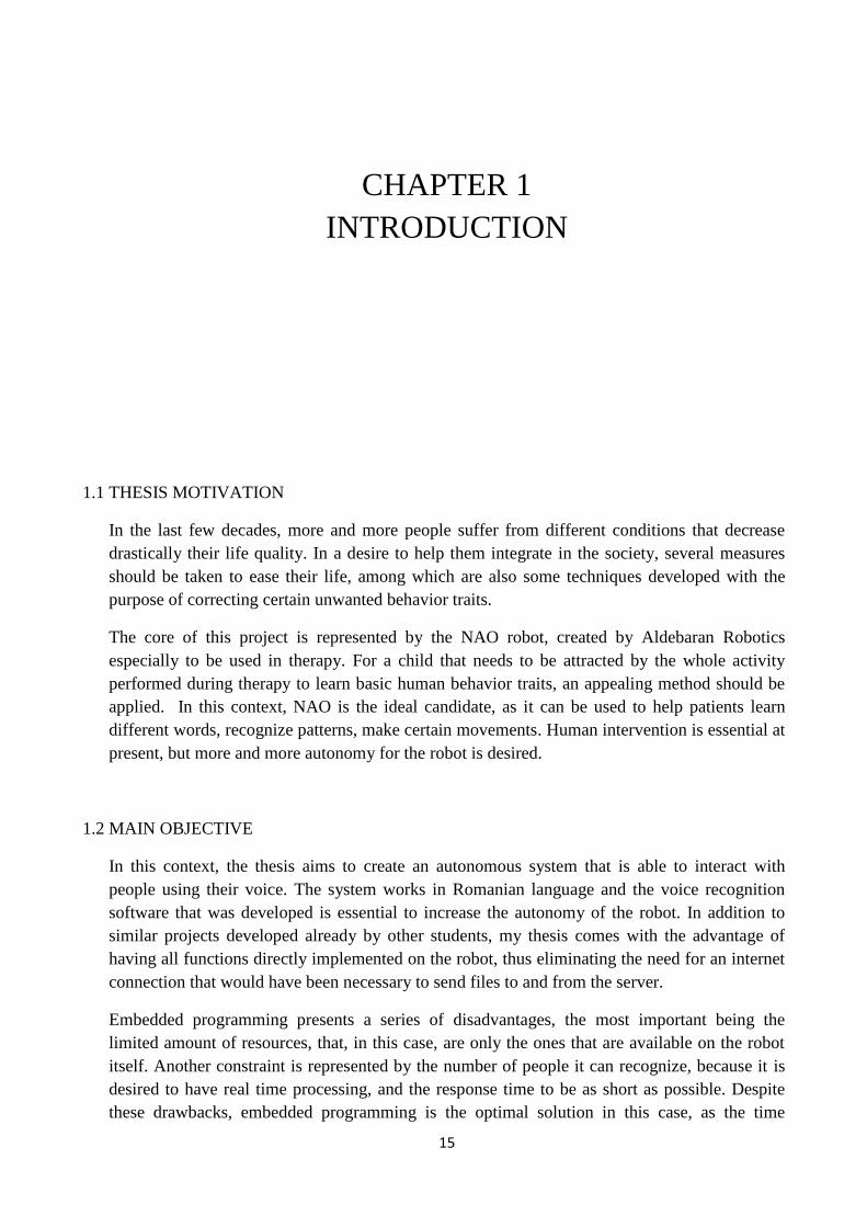
The steps required to reach the proposed objective are represented below:

Figure 1.1 Implementation Steps

1.3 SPECIFIC OBJECTIVES

The objectives this thesis proposes are, as follows:

Collecting data corresponding to several users that will be identified by the robot. Data

is represented by several recordings of the voice of the people that are to be recognized

and it is gathered by the robot itself.

Extracting parameters that define the voice of a single person and map them in a

database, thus being able to uniquely identify people from the restricted set that was

imposed.

Update the database such that the model corresponding to each user gives minimum

errors.

Giving a message to check if the robot recognized the person or not.

Study the effects of noise on the overall results.

Collect data

Filter the recording

Apply algorithm to extract specific

parameters

Make decision

17

Study the variation of the accuracy with the various adjustable parameters in order to

make the best complexity – results compromise.

This thesis is organized in six chapters. Chapter 1 presents the motivation along with the

objectives of the thesis. In Chapter 2 a detailed presentation of the hardware and software

technologies used in the implementation of the project is being made. Chapter 3 describes the

filtering method I applied to the information collected by NAO. In Chapter 4, the voice

recognition algorithm is presented, details regarding each step being given. Chapter 5 presents

the tests made, along with the results obtained for each of the studied cases. In Chapter 6, the

main conclusions of the thesis are drawn and the contributions the author brought to the project

are emphasized, along with some further possible directions.

19

CHAPTER 2

HUMANOID ROBOTS

2.1 GENERAL ASPECTS

A humanoid robot is a robot whose appearance is based on that of the human body. The most

important physical characteristics such a robot has are the head, a torso, two hands and two legs,

with some exceptions regarding earlier versions, when only the superior part of the body was

built. Usually, the head resembles that of a person, having two eyes, a mouth and ears that map

some of its functionalities. [1]

During the last few years, the existence of such robots became more and more a necessity, since

many tasks could be easily carried on by them. The goal is to make the robot autonomous, so

that it can work without any human help. This way, it can complete complex tasks; it can

communicate, learn from people and interact with them.

2.2 APPLICATIONS OF HUMANOID ROBOTS

Since their apparition, many applications have been found for humanoid robots. They could be

successfully used for spatial applications, therapy, quenching flames and other rescue missions,

help with some chores around the house, and so on.

Even though many possible functions are still in research stage, promising results are obtained

in the laboratory. Challenges may occur due to the fact that every ability the robot is expected to

have needs to be carefully programmed and tested. Also, the desire to have an autonomous

system imposes some tougher requirements on the software characteristics.

The term “autonomous” refers to the ability of the robot to perform tasks without being

controlled by humans. The degree of autonomy is increased by self-learning and safe-

developing. [2]

20

2.3 NAO

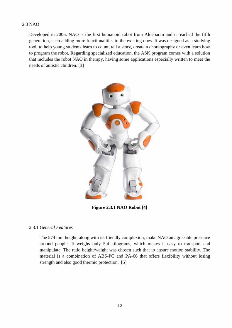
Developed in 2006, NAO is the first humanoid robot from Aldebaran and it reached the fifth

generation, each adding more functionalities to the existing ones. It was designed as a studying

tool, to help young students learn to count, tell a story, create a choreography or even learn how

to program the robot. Regarding specialized education, the ASK program comes with a solution

that includes the robot NAO in therapy, having some applications especially written to meet the

needs of autistic children. [3]

Figure 2.3.1 NAO Robot [4]

2.3.1 General Features

The 574 mm height, along with its friendly complexion, make NAO an agreeable presence

around people. It weighs only 5.4 kilograms, which makes it easy to transport and

manipulate. The ratio height/weight was chosen such that to ensure motion stability. The

material is a combination of ABS-PC and PA-66 that offers flexibility without losing

strength and also good thermic protection. [5]

21

2.3.2 Resources

NAO is equipped with a Lithium-Ion battery, having the nominal capacity of 2.25Ah. The

charging duration is less than three hours and the autonomy is of about 60 minutes. The

robot can be used while it is plugged in. [5]

NAO has a single nucleus processor, ATOM Z530 that is usually utilized for mobile

devices due to its low energy consumption. The CPU has the clock of 1.6 GHz. The 1GB

RAM memory is one of the limitations presented by the robot for real-time applications.

The Flash memory is of 2GB. An 8GB Micro SDHC can be used at maximum. At the

torso level, another processor is used, with the purpose of controlling the actuators.

ARM7TDMI is a 32 bit, RISC microcontroller. [5]

Regarding the connectivity, it can be done via Ethernet or Wi-Fi. The Ethernet port can be

accessed on the back of the head with a RJ45 jack. The speeds supported are 100Mbps,

1000Mbps or 1Gbps. To update the system of the robot, an Arduino device, Kinect or

Asus 3D sensor can be connected through the USB port placed at the back of the head. [5]

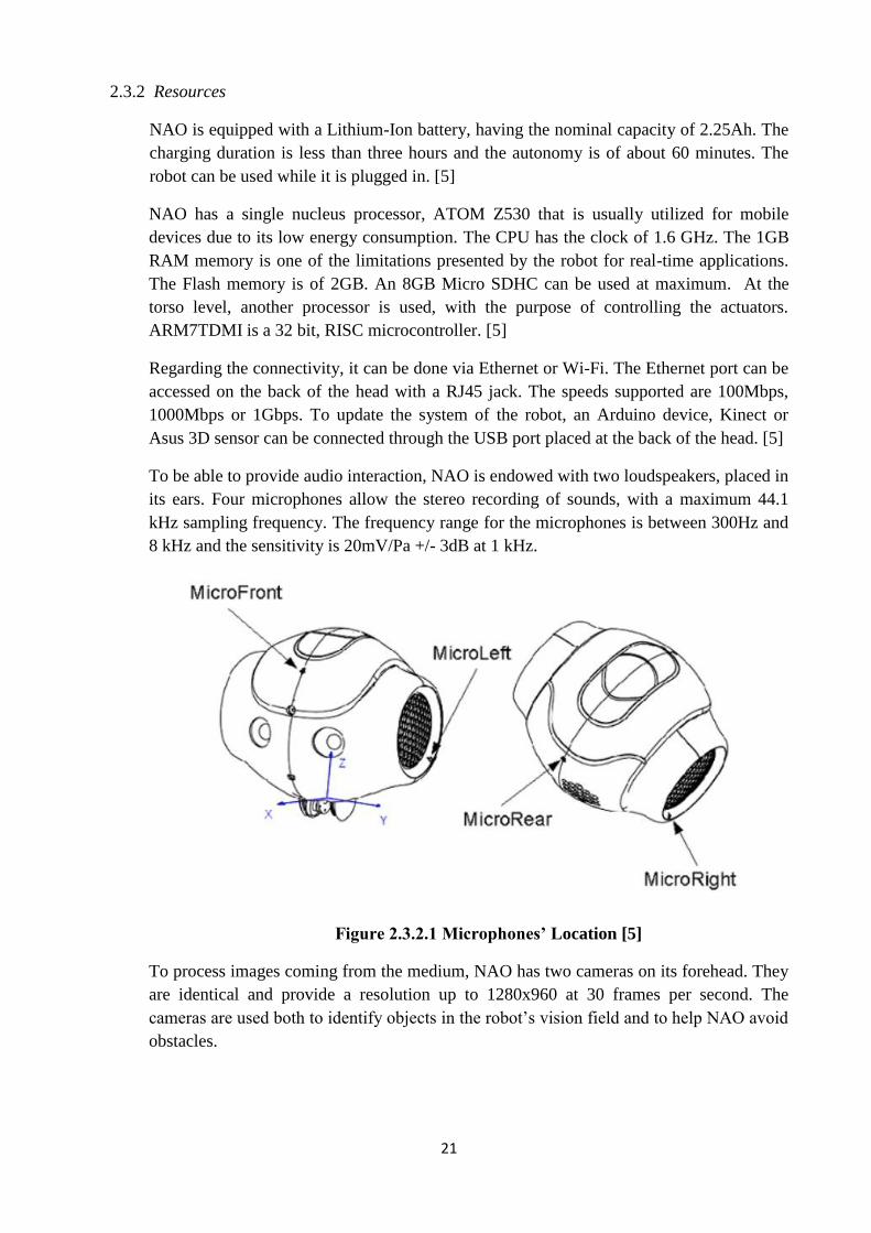
To be able to provide audio interaction, NAO is endowed with two loudspeakers, placed in

its ears. Four microphones allow the stereo recording of sounds, with a maximum 44.1

kHz sampling frequency. The frequency range for the microphones is between 300Hz and

8 kHz and the sensitivity is 20mV/Pa +/- 3dB at 1 kHz.

Figure 2.3.2.1 Microphones’ Location [5]

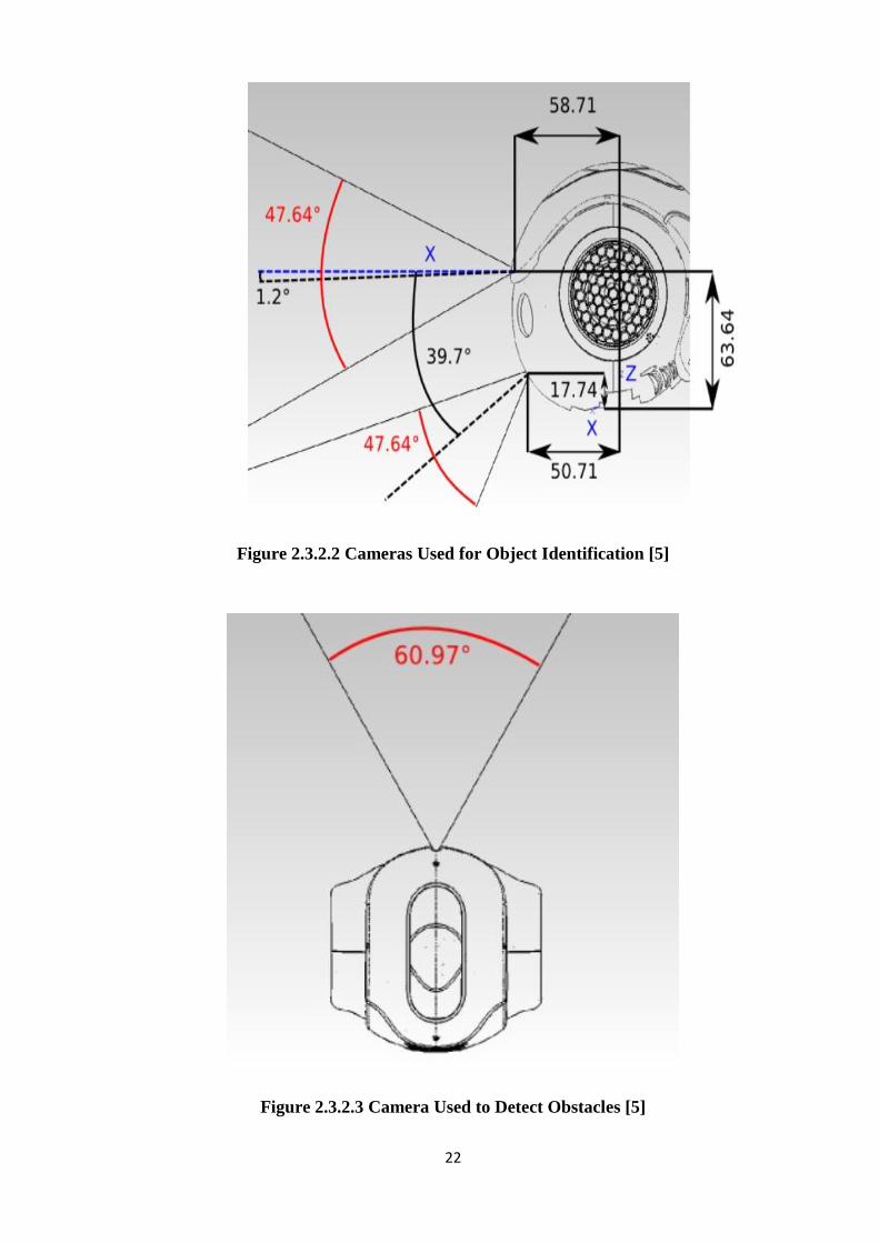
To process images coming from the medium, NAO has two cameras on its forehead. They

are identical and provide a resolution up to 1280x960 at 30 frames per second. The

cameras are used both to identify objects in the robot’s vision field and to help NAO avoid

obstacles.

22

Figure 2.3.2.2 Cameras Used for Object Identification [5]

Figure 2.3.2.3 Camera Used to Detect Obstacles [5]

23

The cameras are of type SOC Image Sensor, model MT9M114. The image array is defined

through the resolution of 1.22 Mp, optical format 1/6 inch and active pixels of 1288x968.

Regarding the sensitivity, the pixel size is 1.9µm*1.9µm. The dynamic range is of 70dB,

while the signal-to-noise ratio is at maximum 37dB. The field of view is 7 .6 DFOV

having 6 .9 the horizontal field of view and 47.6 the vertical one. The focus is of fixed

type and its range starts at 30 cm. The cameras output 1280x960 at 30 frames per second.

The shutter is of type Electronic Rolling Shutter. [5]

NAO has many LEDs that make it pleasant and also can be used to mark some aspects

regarding the functionality. For example, when the eyes turn red, it means that the battery

is low. The LEDs are placed according to the figure:

Figure 2.3.2.4 LED Positions [6]

The LEDs in the ears are all blue. The eyes, chest and feet LEDs are red, green and blue,

which properly combined give the whole color spectrum. Also, the light intensity can be

varied between 0 and 100%.

24

Force sensitive resistances are the sensors that measure the resistance change according to

the pressure applied. They are placed on the robot’s feet. [5]

Figure 2.3.2.5 FSR Sensors [5]

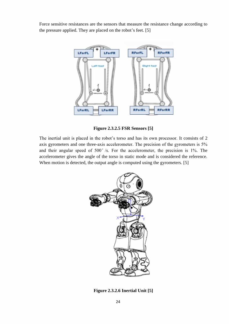
The inertial unit is placed in the robot’s torso and has its own processor. It consists of 2

axis gyrometers and one three-axis accelerometer. The precision of the gyrometers is 5

and their angular speed of 5 s. For the accelerometer the precision is 1 . The

accelerometer gives the angle of the torso in static mode and is considered the reference.

When motion is detected, the output angle is computed using the gyrometers. [5]

Figure 2.3.2.6 Inertial Unit [5]

25

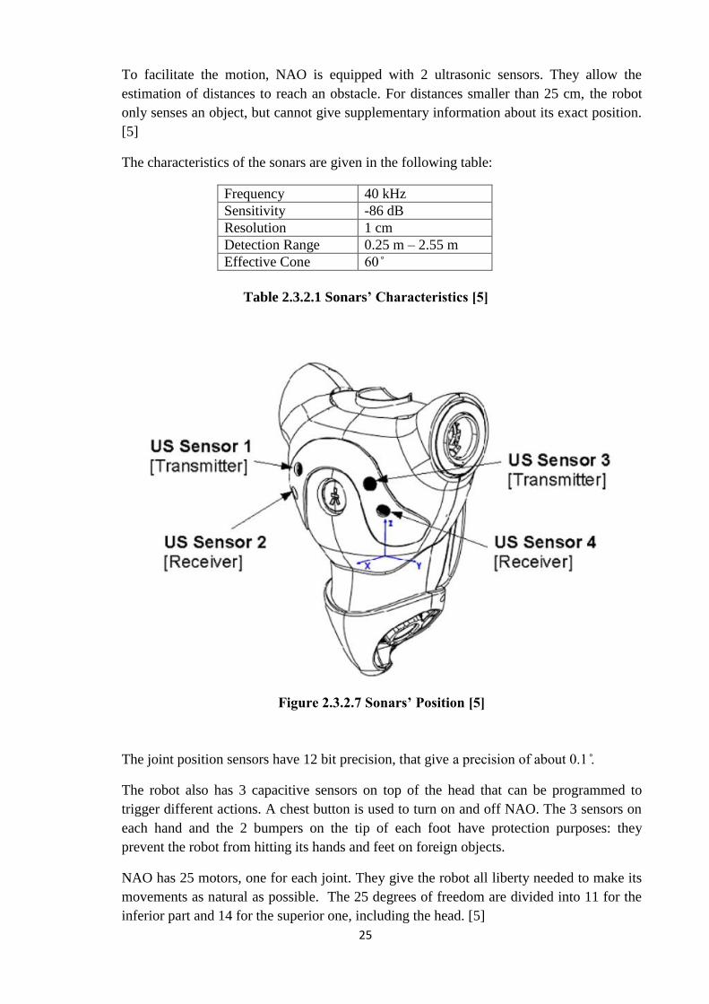
To facilitate the motion, NAO is equipped with 2 ultrasonic sensors. They allow the

estimation of distances to reach an obstacle. For distances smaller than 25 cm, the robot

only senses an object, but cannot give supplementary information about its exact position.

[5]

The characteristics of the sonars are given in the following table:

Frequency 40 kHz

Sensitivity -86 dB

Resolution 1 cm

Detection Range 0.25 m – 2.55 m

Effective Cone 6

Figure 2.3.2.7 Sonars’ Position [5]

The joint position sensors have 12 bit precision, that give a precision of about .1 .

The robot also has 3 capacitive sensors on top of the head that can be programmed to

trigger different actions. A chest button is used to turn on and off NAO. The 3 sensors on

each hand and the 2 bumpers on the tip of each foot have protection purposes: they

prevent the robot from hitting its hands and feet on foreign objects.

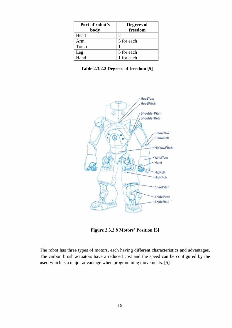
NAO has 25 motors, one for each joint. They give the robot all liberty needed to make its

movements as natural as possible. The 25 degrees of freedom are divided into 11 for the

inferior part and 14 for the superior one, including the head. [5]

Table 2.3.2.1 Sonars’ Characteristics [5]

26

Part of robot’s

body

Degrees of

freedom

Head 2

Arm 5 for each

Torso 1

Leg 5 for each

Hand 1 for each

Figure 2.3.2.8 Motors’ Position [5]

The robot has three types of motors, each having different characteristics and advantages.

The carbon brush actuators have a reduced cost and the speed can be configured by the

user, which is a major advantage when programming movements. [5]

Table 2.3.2.2 Degrees of freedom [5]

27

Motor Type 1 Motor Type 2 Motor Type 3

Model 22NT82213P 17N88208E 16GT83210E

No load speed 8 300 rpm ±10% 8 400 rpm ±12% 10 700 rpm ±10%

Stall torque 68 mNm ±8% 9,4 mNm ±8% 14,3 mNm ±8%

Nominal torque 16.1 mNm 4.9 mNm 6.2 mNm

Table 2.3.2.3 Motor Types [5]

For the legs, motors of type 1 are used, as they are the most powerful from the three. Type

2 are used for the hand joints and type 3 motors for the arms and head.

29

CHAPTER 3

WIENER FILTERING

3.1 GENERAL ASPECTS

The useful speech signal is usually affected by noise, which compromises the results obtained

after processing. In order to minimize the effect it has on the useful signal, some filtering

methods were developed, that help enhance the speech signal.

The Wiener filtering method is one of the most used techniques for signal enhancement. It is

used to produce an estimate of the desired signal, by having as inputs the noisy signal and

assuming that the noise is additive. It minimizes the mean square error between the desired

result and the estimated one. To determine the filter coefficients, the spectral properties of the

original, compromised signal and of the noise should be known. Also, the original signal and the

noise are considered stationary, linear stochastic processes. [7]

3.2 RANDOM SIGNALS AND SPECTRAL DENSITIES [8]

Let x be a discrete time signal, defined as:

x = (….., x-1, x 0, x1,…..);

Its Fourier and Z transforms are

( ) ∑

, -

( ) ∑

30

The correlation function is defined as follows:

( ) ( )

A signal is wide-sense stationary (WSS) if the following conditions are met:

the mean of the signal is constant, time invariant

E[ - , -

the autocorrelation function does not depend on the absolute time, but only on the time

difference between the two moments when it is calculated

( ) ( )

It can be proven that, for WSS signals, the autocorrelation function is even, that is:

( ) ( )

The power spectral density of a WSS signal is:

( ) ∑ ( )

, -

Two WSS stationary processes are joint-WSS if:

( ) ( ) ( )

Their power spectral density:

( ) (

)

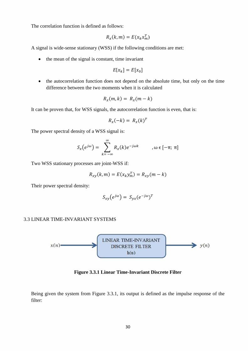
3.3 LINEAR TIME-INVARIANT SYSTEMS

Figure 3.3.1 Linear Time-Invariant Discrete Filter

Being given the system from Figure 3.3.1, its output is defined as the impulse response of the

filter:

31

( ) ∑ ( ) ( )

A linear time-invariant discrete system is stable if its impulse response function is absolutely

summable, that is:

∑ | ( )|

For stable systems, the output in frequency domain is:

( ) ( ) ( )

And, in the z domain,

( ) ( ) ( )

The system is stable if all poles of H(z) are inside the unity circle.

3.4 WIENER FILTER’S COEFFICIENTS [9]

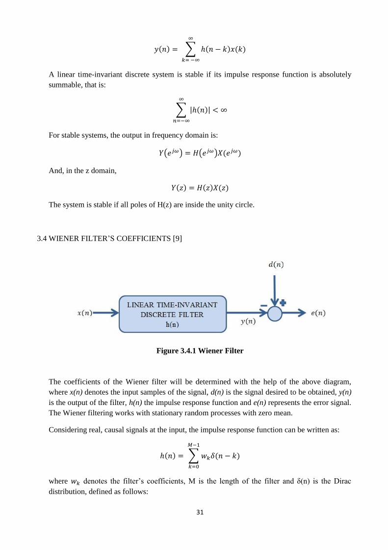
Figure 3.4.1 Wiener Filter

The coefficients of the Wiener filter will be determined with the help of the above diagram,

where x(n) denotes the input samples of the signal, d(n) is the signal desired to be obtained, y(n)

is the output of the filter, h(n) the impulse response function and e(n) represents the error signal.

The Wiener filtering works with stationary random processes with zero mean.

Considering real, causal signals at the input, the impulse response function can be written as:

( ) ∑ ( )

where denotes the filter’s coefficients M is the length of the filter and δ(n) is the Dirac

distribution, defined as follows:

32

δ(k) = {

The output of the filter, y(n), will be:

( ) ∑ ( )

The Wiener filters realize the optimization in the mean-square sense, that is by minimizing the

mean-square error that appears between the output of the filter and the desired signal. In

consequence, the cost function is defined:

*| ( )| + || ( )|| ⟨ ⟩

So the goal is to find the filter’s coefficients for which the cost function is minimal.

In order to do so, the expression of the error function is written:

( ) ( ) ( ) ( ) ∑ ( )

The cost function thus becomes:

* ( ) + *, ( ) ∑ ( )

- +

* ( ) + * ( ) ∑ ( ) +

* ∑ ( )

( ) +

*∑ ( )

∑ ( )

+

The correlation function is:

( ) * ( ) ( )+ * ( ) ( )+

The coefficients of the filter are constants and real, so the mean operator does not affect them.

Taking these into consideration, the cost function becomes:

* ( ) +

∑ * ( ) ( )+

∑ * ( ) ( )+ ∑ ∑

* ( ) ( )+

* ( ) + ∑ ( )

∑ ( ) ∑ ∑

( )

33

With ( ) was denoted the correlation function between the input signal and the desired one

and with ( ) the autocorrelation function of the input signal.

For real valued processes,

( ) ( )

* ( ) + ∑ ( ) ∑ ∑

( )

To write in a matrix form, the following vectors are defined:

w = , -

x(n) = , ( ) ( ) ( -

p = , ( ) ( ) ( )-

R = E{ ( ) ( ) + [ ( ) ( )

( ) ( )]

The cost function in matrix form is:

* ( ) +

The minimum is reached when the gradient is zero. The gradient of a scalar function

f( , ) is defined as:

( ) [

]

By applying this expression to the cost function, and observing that d(n) does not depend on any

w coefficient, it results that:

* + * * ( ) + + *

+ * +

, - [ ( )

( )]

( ) ( ) ( )

( )

34

, - [ ( ) ( )

( ) ( )] [

]

, ( ) ( ) ( )-

, ( ) ( ) ( )-

So,

* +

To minimize the function,

* +

It implies that

The optimal coefficients for the Wiener filter are denoted obtained as:

For optimal coefficients of the filter, an observation regarding the orthogonality of the input

signal with the error can be made.

* ( ) ( )+ * ( ), ( ) ( )-+ * ( ), ( ) ( ) -+

* ( ) ( )+ * ( ) ( ) +

This infers that the input signal and the error signal are uncorrelated.

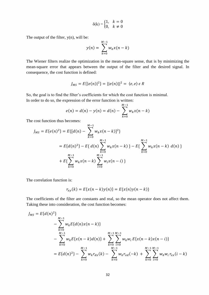
3.5 WIENER FILTER USED IN NOISE REDUCTION

The noise reduction is a particular case of Wiener filtering, where the input is the signal affected

by noise and the desired signal is the noise. The schematics below describes the principle:

Figure 3.5.1 Noise Reduction Using Wiener Filter [10]

35

With s(n) was denoted the useful signal and with v(n) the additive noise; ( ) is the noise at the

output of the filter, that is subtracted from the noisy signal. The Wiener filter tries to make its

output as close as possible to the sum of the desired signal and noise. The correlation between

the noise and the useful signal will be zero, while the noise that is added over the signal will be

strongly correlated with the noise at the output of the filter. So, when subtracting the two

signals, the error signal will be, in fact, the useful signal, without noise.

37

CHAPTER 4

GMM-UBM

4.1 MARKOV CHAINS

The most important machine learning model in speech processing is the hidden Markov model.

In order to be defined, a proper definition for the Markov chain should be given. Markov chains,

as well as the hidden Markov models, are extensions of the finite automata, which are defined

by states and transitions between them. For a weighted finite-state automaton, each arc that

represents a transition between two states is associated with the probability for that transition to

occur. So, the probability of a Markov chain to be in a particular state at a given time depends

only on the state in which the Markov chain previously was. It can be observed that the

probabilities on all arcs leaving a node must be 1. [11]

A Markov chain is a weighted automaton in which the input sequence uniquely determines

which states the automaton will go through. It models a class of random processes that

incorporate a minimum amount of memory.

Considering a sequence of random variables from a discrete alphabet,

* +, by applying the Bayes rule,

( ) ( )∏ ( | )

where .

The random variables X form a first-order Markov chain if ( | ) ( | ), which

means that, for a first-order Markov chain,

( ) ( )∏ ( | ) .

38

This equation is known as the Markov assumption and it uses very little memory to model

dynamic data sequences, as the probability of a random variable at a given time depends only on

the value at the preceding time, regardless of all other previous values. So, the Markov chain

can be used to model stationary signals. [12]

For a Markov chain with N distinct states, having the state at time t in the Markov chain denoted

as , the parameters of the Markov chain are:

( | )

( )

With was denoted the transition probability from state i to state j, while represents the

initial probability for the Markov chain to start from state i. As it is well known, both

transitions’ probabilities and initial probabilities are bounded by constraints that is:

∑

∑

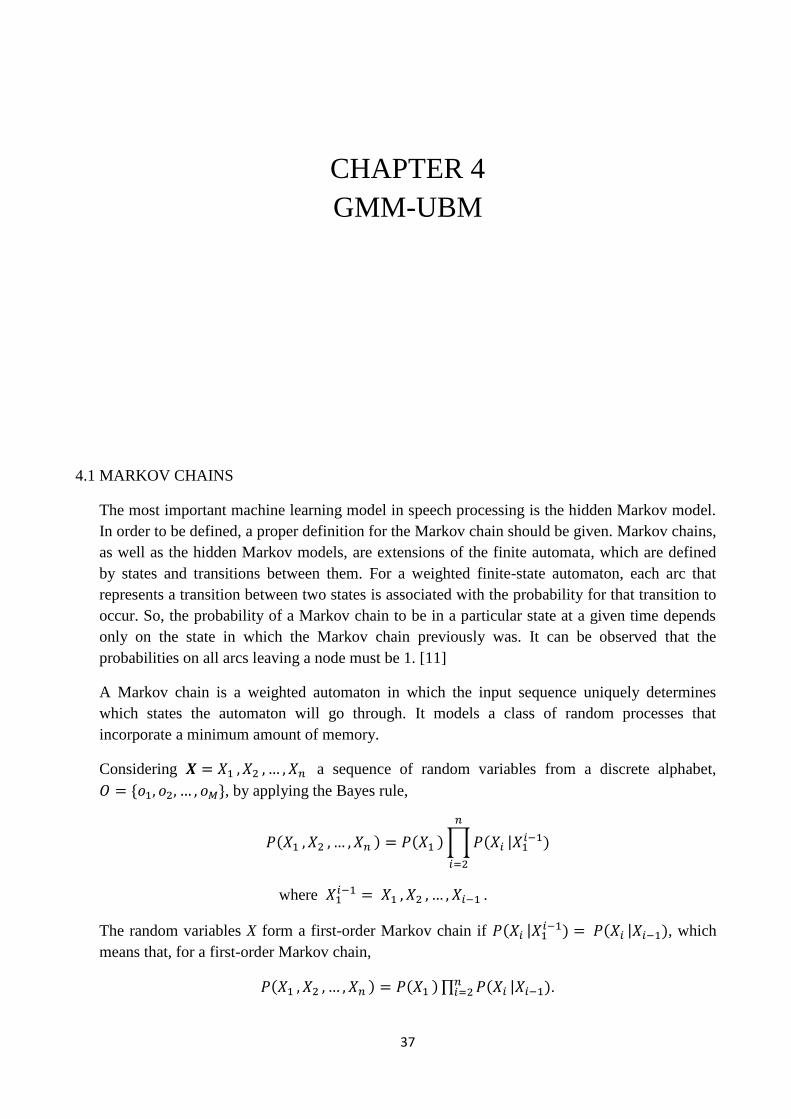
As an example, consider the three-state Markov chain for the Dow Jones Industrial average. At

the end of each day, the Dow Jones Industrial average may correspond to one of the states: [12]

state 1 – up

state 2 – down

state 3 – unchanged

39

Figure 4.1.1 Markov Chain for Dow Jones Industrial Average [12]

The state-transition probability matrix is:

[

]

The initial state probability matrix is:

[ ]

As it can be seen, both probabilities matrices are defined in accordance with the imposed

conditions.

4.2 THE HIDDEN MARKOV MODEL (HMM)

The Markov chain can be used to compute a probability for a sequence of observable events.

Sometimes, the events may not be observable. For example, in speech recognition, acoustic

events are observable and the presence of hidden words that are the underlying causal source of

the acoustics is inferred. A hidden Markov model allows the study of both observed and hidden

events that are thought of as the causal factors in the probabilistic model. [11]

40

A HMM is specified by the following components:

Component Description

a set of N states

a transition probability matrix A, each representing the probability for the transition

from state i to state j to occur

a sequence of T observations, each one drawn

from a vocabulary

( ) a sequence of observation likelihoods, each

expressing the probability of an observation being generated by the state i

a special start state and final state that are not

associated with observations

Table 4.2.1 HMM Components [11]

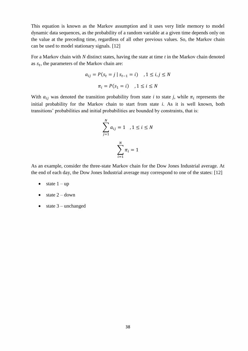
As an example, the task proposed by Jason Eisner will be further treated. A climatologist from

the year 2799 has to study global warming. He cannot find any records concerning the weather

in Baltimore, so he uses the diary of Jason Eisner, where the number of ice creams Jason ate

each day is written down. Using these observations, the temperature for each day needs to be

estimated. As a simplification, only two kinds of days are considered: cold and hot. So, being

given a sequence of observations O (the number of ice creams eaten on a given day), the hidden

sequence Q of weather states should be found. [11]

Figure 4.2.1 HMM for the Ice Cream Task [13]

The two hidden states “hot” and “cold” correspond to hot and cold weather and the

observations correspond to the number of ice creams eaten on a given day.

41

A HMM having non-zero probability of transitioning between any two states is an ergodic

HMM (fully connected). [11]

4.3 HMM TRAINING: BAUM-WELCH ALGORITHM

Being given a set of observations O and the set of possible states in the HMM, the task is to

determine the HMM parameters, that is the A (transition probability matrix) and B (observation

likelihood) matrices.

The algorithm most commonly used to train the HMM is the Baum-Welch algorithm, which is a

special case of Expectation Maximization. The advantage of this algorithm is that it allows the

training of both the transition probabilities and the emission probabilities of the HMM.

If the simpler case of training a Markov chain is considered, since the states are observed, the

model can be run on the observation sequence. As a result, the path taken through the model can

be directly observed and so is the state which generated each observation symbol. A Markov

chain can be in fact considered a hidden Markov model having all the b probabilities equal to 1

for the observed symbol and 0 for all other symbols. So, in this case, only the transmission

probabilities A should be trained.

To obtain the maximum likelihood estimate of the probability of a transition from state i to

state j, the number of times this transition was taken is counted, denoted by ( ). Then, the

normalization to the number of all transitions from state i is performed, and thus is obtained.

This can be done only because the states are already known.

( )

∑ ( )

For a HMM, the counts cannot be computed directly from the observation sequence, since the

path taken through the machine for a specified input is not known. The Baum-Welch algorithm

solves this problem. First of all, the counts are iteratively estimated, that is, starting from an

estimate of the transition and observation probabilities, better and better probabilities are

obtained. Secondly, the estimated probabilities are obtained by computing the forward

probability for an observation and then dividing the probability mass among all the different

paths that contributed to this forward probability. [11]

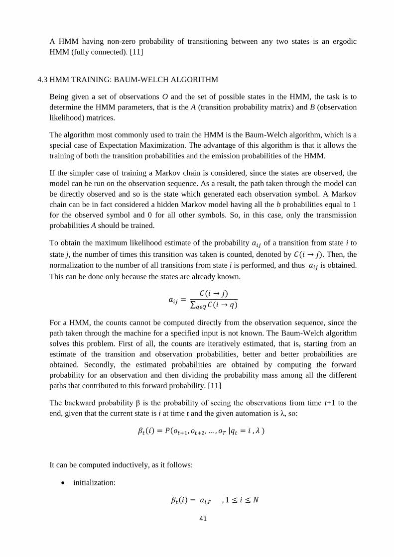
The backward probability β is the probability of seeing the observations from time t+1 to the

end, given that the current state is i at time t and the given automation is λ so:

( ) ( | )

It can be computed inductively, as it follows:

initialization:

( )

42

recursion:

( ) ∑ ( ) ( )

finish:

( | ) ( ) ( ) ∑ ( ) ( )

Now, the estimate transition probability is defined as follows:

Being given the observation sequence and the model, the probability of being in state i at time t

and at state j at time t+1 is defined:

( ) ( | )

To be able to compute , another probability should be first computed, similar to this one but

with a different conditioning for O:

( ) ( | ) ( ) ( ) ( ) , -

Knowing that:

( | ) ( | )

( | )

( | ) ( ) ( ) ∑ ( )

( )

And by introducing these in :

( ) ( ) ( ) ( )

( )

The expected number of transitions from state i to state j is the sum of over the whole t

domain. The total expected number of transitions from state i is the sum of all transitions

coming out of state i. Thus, the final expression is:

∑ ( )

∑ ∑ ( )

43

The probability of a given symbol from the vocabulary V, being given a state j can be

computed using:

( )

The probability of being in state j at time t, ( ), is:

( ) ( | )

By including the observation sequence in the probability:

( ) ( | )

( | ) ( ) ( )

( | )

where by ( ) was denoted the forward probability and by ( ) the

backward probability.

So, knowing that for the numerator the sum of ( ) for all time steps when the observation

was the symbol , and for the denominator the sum of ( ) for all time steps t should be

computed, the expression for ( ) becomes:

( ) ∑ ( )

∑ ( )

Now, the transition A and observation B probabilities from an observation sequence O can be re-

estimated, assuming that at the beginning there are already some previous estimates for A and B,

which represent the initial estimate of the HMM parameters for the forward-backward

algorithm. Then, the steps are run iteratively. There are two major steps:

expectation step where the expected state occupancy count γ and the expected state

transition count ξ are computed from the old A and B probabilities

maximization step, where the new A and B probabilities are computed from γ and ξ

4.4 HMM APPLIED TO SPEECH

The principles when using HMM for speech recognition are the same as the ones from the

examples given before, but for the observation sequence, which in this case is a sequence of

acoustic feature vectors. Each one of these acoustic feature vectors gives information about the

amount of energy in different frequency bands at each point in the time domain. Each

observation contains, in fact, a vector of 39 real-valued features that give information about the

spectrum of the signal. [11]

When choosing the hidden states of the hidden Markov model, the number of words used for the

database creation is extremely important. For small tasks, that is, a small number of words, the

44

hidden states correspond to entire words. If the number of words increases, the hidden states in

the HMM correspond to smaller units, that are called phones. The phone is defined as “the

smallest identifiable unit found in a stream of speech that is able to be transcribed” [14]. This

way, for larger tasks, the words are considered a sequence of phones, so a word HMM consists

of a stream of HMM states. [11]

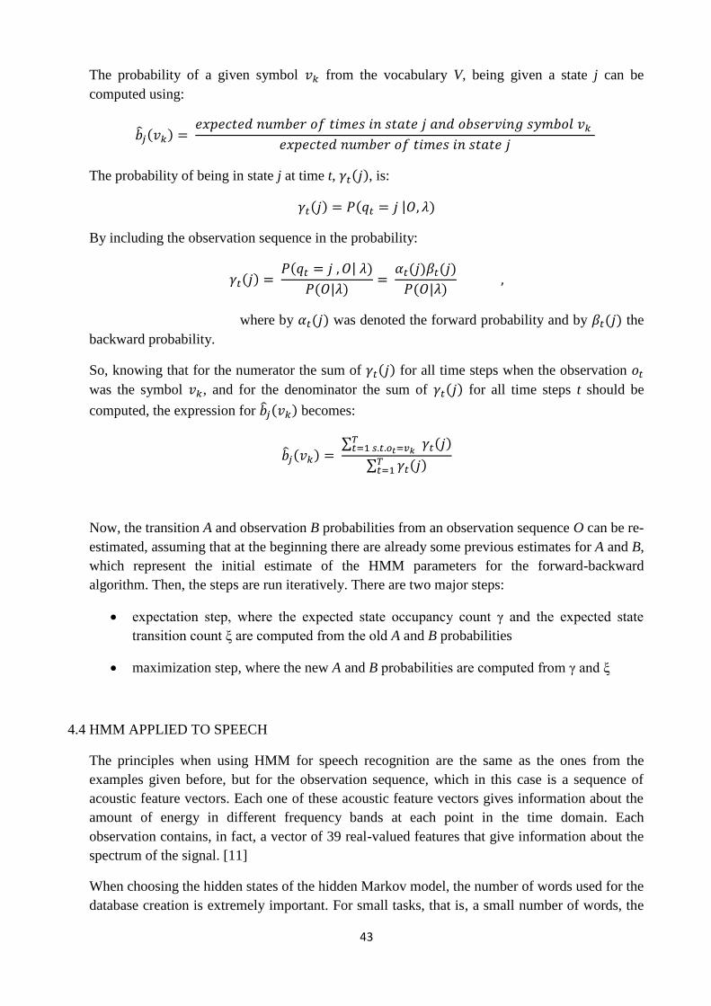
A major aspect that differentiates the HMM models for speech recognition from other HMM

models is the forbiddance of arbitrary transitions. Strong constraints on transitions are imposed,

based on the sequential nature of speech. So, states can transition to themselves or to the next

state only. This special HMM structure is named Bakis network and is the most common model

used for speech.

Figure 4.4.1 Bakis Model [15]

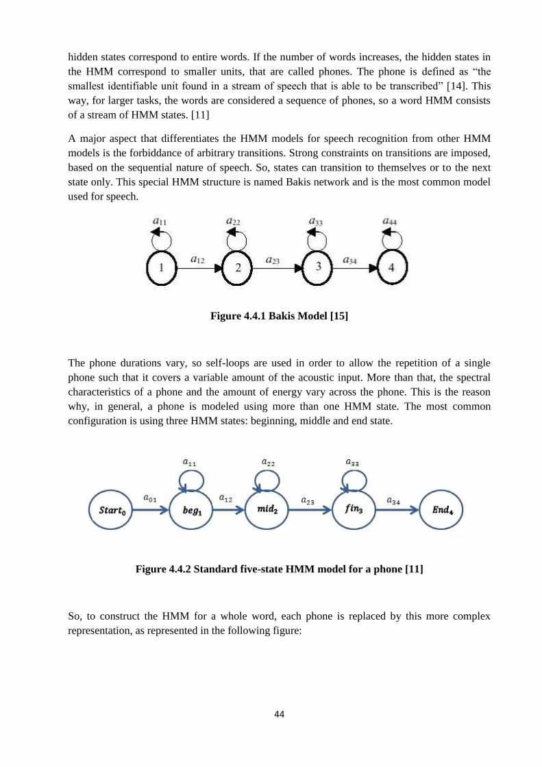
The phone durations vary, so self-loops are used in order to allow the repetition of a single

phone such that it covers a variable amount of the acoustic input. More than that, the spectral

characteristics of a phone and the amount of energy vary across the phone. This is the reason

why, in general, a phone is modeled using more than one HMM state. The most common

configuration is using three HMM states: beginning, middle and end state.

Figure 4.4.2 Standard five-state HMM model for a phone [11]

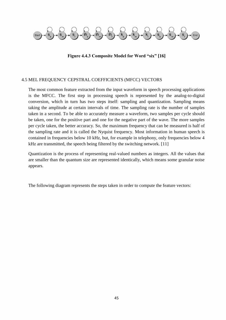
So, to construct the HMM for a whole word, each phone is replaced by this more complex

representation, as represented in the following figure:

45

Figure 4.4.3 Composite Model for Word “six” [16]

4.5 MEL FREQUENCY CEPSTRAL COEFFICIENTS (MFCC) VECTORS

The most common feature extracted from the input waveform in speech processing applications

is the MFCC. The first step in processing speech is represented by the analog-to-digital

conversion, which in turn has two steps itself: sampling and quantization. Sampling means

taking the amplitude at certain intervals of time. The sampling rate is the number of samples

taken in a second. To be able to accurately measure a waveform, two samples per cycle should

be taken, one for the positive part and one for the negative part of the wave. The more samples

per cycle taken, the better accuracy. So, the maximum frequency that can be measured is half of

the sampling rate and it is called the Nyquist frequency. Most information in human speech is

contained in frequencies below 10 kHz, but, for example in telephony, only frequencies below 4

kHz are transmitted, the speech being filtered by the switching network. [11]

Quantization is the process of representing real-valued numbers as integers. All the values that

are smaller than the quantum size are represented identically, which means some granular noise

appears.

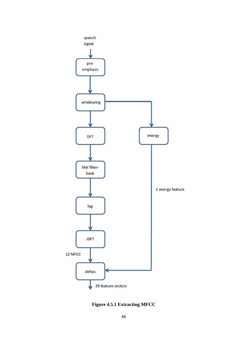
The following diagram represents the steps taken in order to compute the feature vectors:

46

Figure 4.5.1 Extracting MFCC

47

4.5.1 Pre-emphasis

Pre-emphasis is the first step in MFCC feature extraction. It is done due to the fact that it

can be observed that the energy for vowels is concentrated on low frequencies and at high

frequencies it drops. So, by boosting the high frequency energy, the phone detection

accuracy is increased. [11]

4.5.2 Windowing

Because the spectral characteristics of the voice signal are not constant in time, it is said

that the speech is a non-stationary signal. To be able to extract spectral features, a

stationary signal is required. A stationary portion of speech is extracted by using a window

which is non-zero inside some region and zero elsewhere.

A windowing process is characterized by:

the width of the window, in milliseconds

the offset between successive windows

the shape of the window

The speech extracted from each window is called a frame, the frame size is represented by

the number of milliseconds in a frame and the frame shift is the number of milliseconds

between the left edges of two successive frames. [11]

Figure 4.5.2.1 Windowing Process for Frame Shift of 10ms and Frame Size of 25ms

[11]

48

To extract the signal y[n], the value of the input signal, s[n], is multiplied by the value of

the window, w[n]:

, - , - , -

The simplest window is the rectangular window, defined as:

, - {

However, problems occur when using the rectangular window due to the abrupt slope that

causes discontinuities, thus creating problems when computing the Fourier transform. This

inconvenience led to the usage of the Hamming window when extracting the MFCC. It

diminishes the values of the signal towards zero at the window boundaries, and at the

same time avoids the appearance of discontinuities. The Hamming window is defined:

, - { (

)

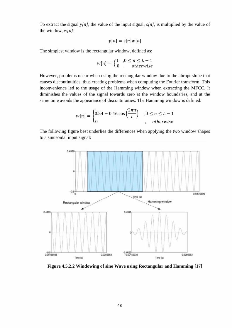
The following figure best underlies the differences when applying the two window shapes

to a sinusoidal input signal:

Figure 4.5.2.2 Windowing of sine Wave using Rectangular and Hamming [17]

49

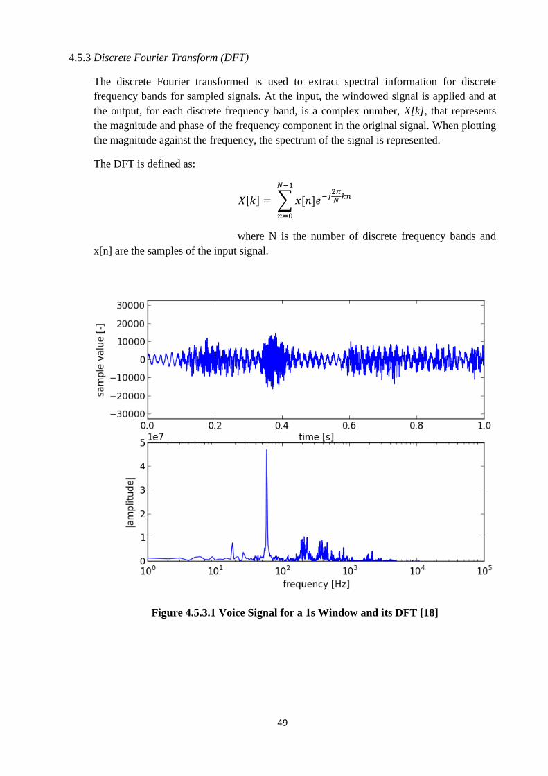
4.5.3 Discrete Fourier Transform (DFT)

The discrete Fourier transformed is used to extract spectral information for discrete

frequency bands for sampled signals. At the input, the windowed signal is applied and at

the output, for each discrete frequency band, is a complex number, X[k], that represents

the magnitude and phase of the frequency component in the original signal. When plotting

the magnitude against the frequency, the spectrum of the signal is represented.

The DFT is defined as:

, - ∑ , -

where N is the number of discrete frequency bands and

x[n] are the samples of the input signal.

Figure 4.5.3.1 Voice Signal for a 1s Window and its DFT [18]

50

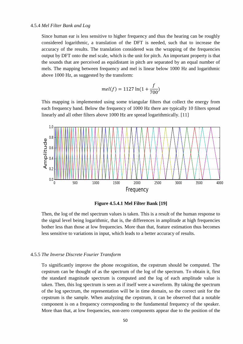
4.5.4 Mel Filter Bank and Log

Since human ear is less sensitive to higher frequency and thus the hearing can be roughly

considered logarithmic, a translation of the DFT is needed, such that to increase the

accuracy of the results. The translation considered was the wrapping of the frequencies

output by DFT onto the mel scale, which is the unit for pitch. An important property is that

the sounds that are perceived as equidistant in pitch are separated by an equal number of

mels. The mapping between frequency and mel is linear below 1000 Hz and logarithmic

above 1000 Hz, as suggested by the transform:

( ) (

)

This mapping is implemented using some triangular filters that collect the energy from

each frequency band. Below the frequency of 1000 Hz there are typically 10 filters spread

linearly and all other filters above 1000 Hz are spread logarithmically. [11]

Figure 4.5.4.1 Mel Filter Bank [19]

Then, the log of the mel spectrum values is taken. This is a result of the human response to

the signal level being logarithmic, that is, the differences in amplitude at high frequencies

bother less than those at low frequencies. More than that, feature estimation thus becomes

less sensitive to variations in input, which leads to a better accuracy of results.

4.5.5 The Inverse Discrete Fourier Transform

To significantly improve the phone recognition, the cepstrum should be computed. The

cepstrum can be thought of as the spectrum of the log of the spectrum. To obtain it, first

the standard magnitude spectrum is computed and the log of each amplitude value is

taken. Then, this log spectrum is seen as if itself were a waveform. By taking the spectrum

of the log spectrum, the representation will be in time domain, so the correct unit for the

cepstrum is the sample. When analyzing the cepstrum, it can be observed that a notable

component is on a frequency corresponding to the fundamental frequency of the speaker.

More than that, at low frequencies, non-zero components appear due to the position of the

51

tongue and other articulators. So, to detect phones only the low frequency components are

needed and to detect the pitch the higher cepstral values are required.

It was observed that the cepstral coefficients have the property that the variance of

different coefficients is uncorrelated in general. This is the main reason for working with

cepstral coefficients instead directly on the spectrum, where the spectral coefficients at

different frequency bands are correlated.

Formally, the cepstrum is defined as the inverse discrete Fourier transform of the log

magnitude of the discrete Fourier transform of the signal, so, for a windowed signal x[n],

the following expression is employed:

, - ∑ (|∑ , -

|)

4.5.6 Deltas and Energy

The cepstral coefficients are obtained for each frame and typically only the first 12 of

them are kept. Next, some other features are added. The energy from the frame correlates

with the phone identity so it is an useful feature in phone detection. The energy in a frame

is computed as the sum over time of the power of the samples in the frame. So, for a signal

x, in a window starting from sample and ending at sample , the energy is computed

as: [11]

∑ , -

The speech signal differs from frame to frame, so the nature of the change from a stop

closure to a stop burst may provide some supplementary information regarding the pitch

identity. In order to obtain this new information, for each feature previously discussed

(cepstral coefficients and energy) a delta and a double delta feature is added. Delta or

velocity features represent the change between frames in the corresponding cepstral or

energy feature. Double delta or acceleration features represent the change between frames

in the corresponding delta features. [11]

So, after adding all new features, the MFCC features are obtained. The most useful

characteristic of the MFCC features is that the cepstral coefficients tend to be uncorrelated, so a

simplification of the acoustic model occurs.

52

4.6 GAUSSIAN MIXTURE MODEL (GMM)

Modern speech recognition algorithms are based on computing observation probabilities

directly on the real-valued, continuous input vector. These models are based on the computation

of the probability density function (PDF) over a continuous space, the most common model

being GMM PDFs. [11]

4.6.1 Univariate Gaussians

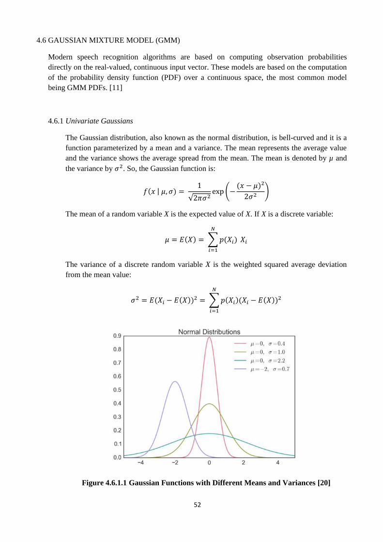
The Gaussian distribution, also known as the normal distribution, is bell-curved and it is a

function parameterized by a mean and a variance. The mean represents the average value

and the variance shows the average spread from the mean. The mean is denoted by µ and

the variance by . So, the Gaussian function is:

( | )

√ (

( )

)

The mean of a random variable X is the expected value of X. If X is a discrete variable:

( ) ∑ ( )

The variance of a discrete random variable X is the weighted squared average deviation

from the mean value:

( ( )) ∑ ( )( ( ))

Figure 4.6.1.1 Gaussian Functions with Different Means and Variances [20]

53

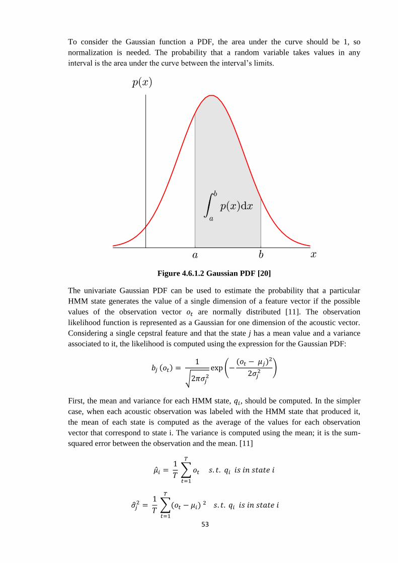
To consider the Gaussian function a PDF, the area under the curve should be 1, so

normalization is needed. The probability that a random variable takes values in any

interval is the area under the curve between the interval’s limits.

Figure 4.6.1.2 Gaussian PDF [20]

The univariate Gaussian PDF can be used to estimate the probability that a particular

HMM state generates the value of a single dimension of a feature vector if the possible

values of the observation vector are normally distributed [11]. The observation

likelihood function is represented as a Gaussian for one dimension of the acoustic vector.

Considering a single cepstral feature and that the state j has a mean value and a variance

associated to it, the likelihood is computed using the expression for the Gaussian PDF:

( )

√

( ( )

)

First, the mean and variance for each HMM state, , should be computed. In the simpler

case, when each acoustic observation was labeled with the HMM state that produced it,

the mean of each state is computed as the average of the values for each observation

vector that correspond to state i. The variance is computed using the mean; it is the sum-

squared error between the observation and the mean. [11]

∑

∑( )

54

In reality, because the states are hidden in HMM, it is impossible to know exactly which

observation vector was produced by which state. So, each observation vector is assigned to

every possible state, given that the HMM was in state i at time t. The probability of being

in state i at time t was already presented as part of the Baum-Welch algorithm and it was

denoted by ( ). As previously discussed, Baum-Welch is an iterative algorithm, so ( )

is computed also iteratively because, by getting a better observation probability b, a better

probability of being in a state i at a given time is obtained. Taking all these into account,

the expressions for the mean and variance become:

∑ ( )

∑ ( )

∑ ( ) ( )

∑ ( )

These two expressions are used in the Baum-Welch algorithm, to train the HMM. Initially,

the values for and are set to some estimates and then recomputed at each step. [11]

4.6.2 Multivariate Gaussians

The use of a multivariate Gaussian is necessary, due to the fact that the acoustic

observation is a vector of 39 features. The multivariate Gaussian allows the assignment of

a probability to a vector. The multivariate Gaussian is defined by a mean vector of D

elements, D being the number of features, and a covariance matrix ∑:

( | ∑)

( ) |∑|

(

( ) ∑ ( ))

The covariance matrix ∑ contains the variance of all dimensions and the covariance

between any two dimensions.

∑ [( ( ))( ( ))] ∑ ( )( ( ))(

( ))

So, the multivariate Gaussian probability estimate for a given HMM, characterized by

and ∑ , is:

( )

( ) |∑|

(

( )

∑ ( ))

The covariance matrix shows the variance between each pair of feature dimensions. If the

features in different dimensions are uncorrelated, ∑ becomes a diagonal matrix, so non-

zero elements are placed along the main diagonal. [11]

55

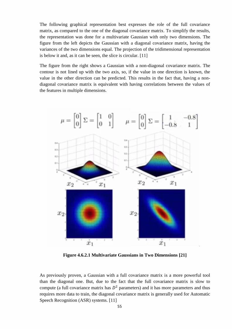
The following graphical representation best expresses the role of the full covariance

matrix, as compared to the one of the diagonal covariance matrix. To simplify the results,

the representation was done for a multivariate Gaussian with only two dimensions. The

figure from the left depicts the Gaussian with a diagonal covariance matrix, having the

variances of the two dimensions equal. The projection of the tridimensional representation

is below it and, as it can be seen, the slice is circular. [11]

The figure from the right shows a Gaussian with a non-diagonal covariance matrix. The

contour is not lined up with the two axis, so, if the value in one direction is known, the

value in the other direction can be predicted. This results in the fact that, having a non-

diagonal covariance matrix is equivalent with having correlations between the values of

the features in multiple dimensions.

Figure 4.6.2.1 Multivariate Gaussians in Two Dimensions [21]

As previously proven, a Gaussian with a full covariance matrix is a more powerful tool

than the diagonal one. But, due to the fact that the full covariance matrix is slow to

compute (a full covariance matrix has parameters) and it has more parameters and thus

requires more data to train, the diagonal covariance matrix is generally used for Automatic

Speech Recognition (ASR) systems. [11]

56

So, with this assumption, the covariance matrix becomes:

∑ [

]

And, introducing in the expression for the likelihood, the following simplification is

obtained:

( ) ∏

√

(

( )

)

To train such a multivariate Gaussian, the same steps as for the univariate Gaussian are

taken. Again, the Baum-Welch algorithm is used, having in mind that ( ) is the

likelihood of being in state i at time t. The same equations are employed, except that now

the observation is a vector of cepstral features, the mean vector is a vector of cepstral

means and the variance vector is a vector of cepstral variances:

∑ ( )

∑ ( )

∑ ( )( ) ( )

∑ ( )

4.6.3 Gaussian Mixture Models - Motivation

As it was previously shown, a multivariate Gaussian can be used to model each dimension

of the feature vector as a normal distribution. Generally, a cepstral feature is not normally

distributed; for this reason, the observation likelihood is modeled with a weighted mixture

of multivariate Gaussians. Such a model is called a Gaussian mixture model. [11] GMM

has become the standard classifier for text-independent speaker recognition due to its

ability to form smooth approximations to arbitrary shaped distributions. Another

advantage is that the training is fast as compared to other methods. [22]

Since HMM is hard to be applied to text-independent speaker recognition, and even so the

improvement is not significant, GMM became the most used model. [23]

In GMM, the speaker model consists of a finite mixture of multivariate Gaussian

components. A mixture density is the weighted sum of M component densities. [24]

( | ) ∑ ( )

where is a D dimensional random vector, are the

mixture weights and ( ) are the component densities.

57

Each component density is:

( )

( ) |∑ |

(

( )

∑ ( ) )

where is the mean vector and ∑ is the covariance matrix.

The constraint imposed on the mixture weights is:

∑

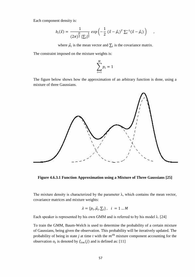
The figure below shows how the approximation of an arbitrary function is done, using a

mixture of three Gaussians.

Figure 4.6.3.1 Function Approximation using a Mixture of Three Gaussians [25]

The mixture density is characterized by the parameter λ which contains the mean vector,

covariance matrices and mixture weights:

* ∑ +

Each speaker is represented by his own GMM and is referred to by his model λ. [24]

To train the GMM, Baum-Welch is used to determine the probability of a certain mixture

of Gaussians, being given the observation. This probability will be iteratively updated. The

probability of being in state j at time t with the mixture component accounting for the

observation is denoted by ( ) and is defined as: [11]

58

( ) ∑ ( ) ( ) ( )

( )

Using the values from the previous iteration, the mean, mixture weight and covariance are

recomputed:

∑ ( )

∑ ∑ ( )

∑ ( )

∑ ∑ ( )

∑ ∑ ( )( )( )

∑ ∑ ( )

There are two main reasons why GMM is used in speaker recognition applications. The

first one is that GMM may model some underlying set of acoustic classes, which represent

some phonetic events, such as vowels, nasals or fricatives. They represent some speaker-

dependent features that are useful in speaker identification. The second reason was

obtained through repeated observations and as it was concluded, a linear combination of

Gaussian basis functions offers the possibility to represent a large class of sampled

distributions. Any arbitrarily-shaped function can be well approximated through GMM.

[24]

Another important characteristic is that, even though there might be some correlation

between the features, full covariance matrices are not needed. Correlations between

feature vector elements can be modeled using a linear combination of diagonal covariance

Gaussians.

4.6.4 Maximum Likelihood Parameter Estimation

The goal of speaker recognition model is to estimate the GMM parameters that best match

the distribution of training feature vectors. The most used method to reach this imposed

target is the maximum likelihood estimation. Maximum likelihood estimation aims to

determine the model parameters that maximize the likelihood of the GMM, when the

training data is already given.

Considering T training vectors, X = { + , the GMM likelihood is:

( | ) ∏ ( | )

Seeing that this expression cannot be maximized directly, as it is a nonlinear function of

the parameters λ, the maximum likelihood estimation is obtained iteratively, using the

particular case of expectation-maximization (EM) algorithm.

59

EM algorithm starts with an initial model λ and estimates a new model such that the

following condition is fulfilled:

( | ) ( | )

After this step, the newly obtained model becomes the initial one for the next iteration and

the process repeats until some threshold is reached. As it can be observed, the principles

are the same as in the case of Baum-Welch algorithm, used to estimate HMM parameters.

[24]

At each iteration, the weight, mean and variance are updated using:

∑ ( | )

∑ ( | )

∑ ( | )

∑ ( | )

∑ ( | )

With , and are denoted the elements from the vectors

, and .

The a posteriori probability for a class i is determined using:

( | ) ( )

∑ ( )

Two important steps that are taken when training the Gaussian mixture model are the

selection of the order M of the mixture and the initialization of parameters for the

estimation maximization algorithm. Since there is no theoretical background to impose

when choosing these parameters, they are application dependent and the values are

selected through repeated experiments. [24]

Usually, the X feature vectors are assumed independent, so the logarithm of the

conditional probability is computed:

( ( | )) ∑ ( ( | ))

( | ) is computed as previously stated,

( | ) ∑ ( )

Sometimes, a normalization through the division by T is necessary; this can be considered

a rough compensation factor to the likelihood value. [26]

60

4.7 UNIVERSAL BACKGROUND MODEL (UBM)

The UBM is “a model in speaker verification system to represent general person-independent,

channel independent feature characteristics to be compared against a model of speaker specific

feature characteristics when making an accept or reject decision”. [23]

The UBM acts as a prior model in maximum a posteriori (MAP) parameter estimation and it is

trained using samples from many speakers, in order to have some general speech characteristics.

Since there is no possibility to determine the optimal number of speakers or speech samples to

be used when training the UBM, the simplest method is to pool all data using EM algorithm.

This is done in order to avoid the dominance of one subpopulation over the others.

4.7.1 Adaptation of Speaker Model

Unlike the standard approach of maximum likelihood training of a model independently

on the UBM, the adaptation procedure is used to continuously update the parameters in the

UBM. This method drastically increases the performances since the speaker’s model and

the UBM are tightly connected.

The adaptation is performed in two steps. In the first step, for each mixture in the UBM,

the estimates of the sufficient statistics of the speaker’s training data are computed. The

sufficient statistics are the basic statistics needed in order to compute the desired

parameters. In the second step, the new results are combined with the old ones using a

data-dependent mixing coefficient. This coefficient is chosen such that, when there is

enough data the new sufficient statistics are more reliable for final parameter estimation,

and when the data count is low, the final result relies more on the a priori information. [26]

Being given an UBM and the training vectors * +, the probabilistic alignment

of the training vectors in the UBM mixture is first determined. For mixture i, the

probabilistic alignment is:

( | ) ( )

∑ ( )

Then, this probabilistic alignment is used to compute the sufficient statistics for weight,

mean and variance:

∑ ( | )

( )

∑ ( | )

( )

∑ ( | )

61

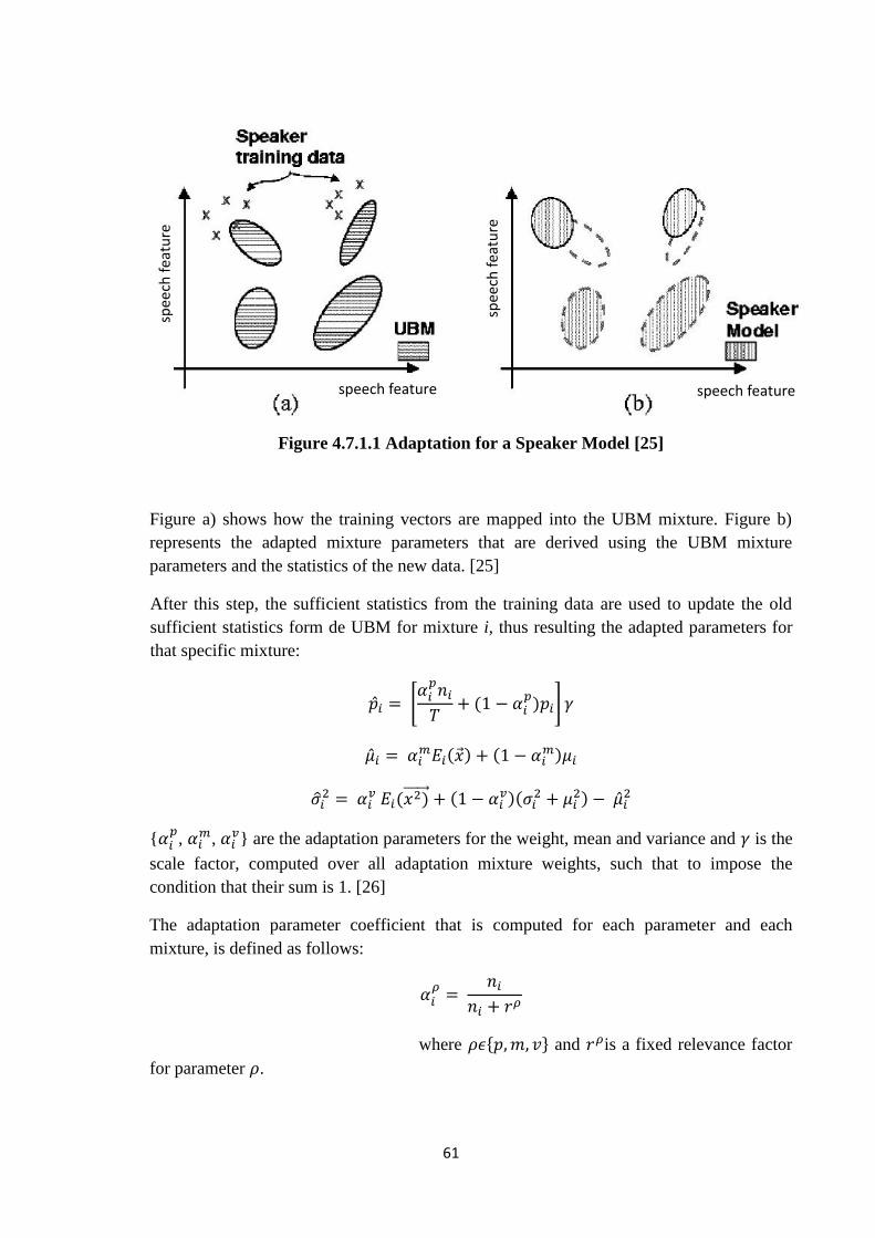
Figure 4.7.1.1 Adaptation for a Speaker Model [25]

Figure a) shows how the training vectors are mapped into the UBM mixture. Figure b)

represents the adapted mixture parameters that are derived using the UBM mixture

parameters and the statistics of the new data. [25]

After this step, the sufficient statistics from the training data are used to update the old

sufficient statistics form de UBM for mixture i, thus resulting the adapted parameters for

that specific mixture:

*

( ) +

( ) (

)

( ) ( )(

)

{ ,

, } are the adaptation parameters for the weight, mean and variance and is the

scale factor, computed over all adaptation mixture weights, such that to impose the

condition that their sum is 1. [26]

The adaptation parameter coefficient that is computed for each parameter and each

mixture, is defined as follows:

where * + and is a fixed relevance factor

for parameter .

speech feature speech feature

spee

ch f

eatu

re

spee

ch f

eatu

re

62

If the probabilistic count, , is low for a specific mixture component, it will make

. This, in turn, leads to a de-emphasis of the new parameters, thus giving the old

parameters more weight. For mixture components with high probabilistic count, ,

so the new speaker-parameters are prioritized over the a priori parameters. Through the

relevance factor the amount of new data to be observed in a mixture before the replacing

of old parameters with the new ones is controlled.

The experiments carried out by Vuuren in his Ph.D. thesis “Speaker Verification in a

Time-Feature Space” proved that the gain when using parameter-dependent adaptation

coefficients is insignificant. [27] So, in most GMM-UBM system, a single adaptation

coefficient for all parameters is used, having the relevance factor 16. Vuuren’s

experiments show similar performances for relevance factors in the range [8-20].

The adaptation approach provides by far better results as compared to the method in which

the speaker model is trained independently on the UBM. If the UBM is considered the

covering space of speaker-independent acoustic classes the adaptation is “the speaker-

dependent tuning of those acoustic classes observed in the speaker’s training speech”. [26]

During the recognition stage, the classes unseen in the speaker training produce zero log-

likelihood ratio values, that are this way not taken into account in the decision making

process.

4.7.2 Log-Likelihood Ratio Computation

For a sequence of feature vectors X, the log-likelihood ratio is computed as:

( ) ( | ) ( | )

Since the hypothesized speaker model was adapted from the UBM, the method works

faster than evaluating separately two GMMs. This is due to the fact that, when evaluating

a large GMM for a feature vector, only a few of the mixtures yield significantly to the

likelihood value. The GMM is represented over a large space, but only few components

are near a single vector. [26]

Another observation that was made is that the vectors that are close to a particular mixture

in the UBM are also close to the corresponding mixture in the speaker model. So, having

these two properties in mind, an improvement in the latency of the response is obtained.

[26]

Following all the steps described in this chapter, the diagram below represents the method

implemented in order to obtain the desired result:

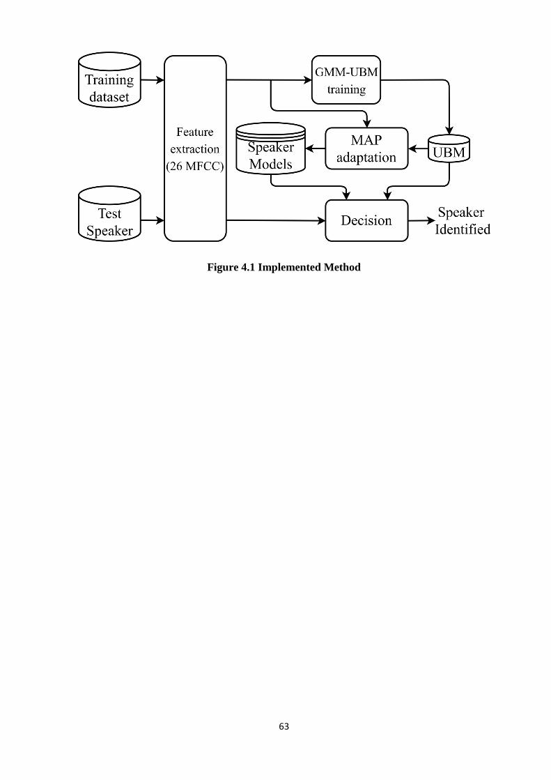
63

Figure 4.1 Implemented Method

65

CHAPTER 5

TESTING THE METHOD

5.1 DATABASE

To create the database used to test the algorithm, a set of 5 speakers was used. For each speaker,

20 voice commands were recorded 10 times each, from different distances and positions relative

to the robot’s microphones in order to have a more accurate model of the speech for the users.

The algorithm developed is text dependent, meaning that the same commands that were used for

training the model should be used in the testing phase.

The 5 speakers chosen were two males and three females, such that to have some diversity. The

recordings were done in a nosy environment, in order to study the effect of noise on the overall

accuracy. The 10 recordings for each command were further divided as follows:

5 recordings for distances below 1 meter

5 recordings for distances greater than 1 meter

Each of these recordings was done from a different position relative to the robot.

The channel is stereo, the recording being done on 2 of the 4 microphones available on the

robot, the ones placed on the right and left side of its head. This decision was made after

studying the quality of some test recordings from each microphone.

5.2 EXPERIMENTAL SETUP

The database thus obtained was divided into:

75% of the recordings were used for training

25% of the recordings were used for testing

66

To make the choice of optimal parameters, it was studied the effect of the sampling rate and

number of Gaussian components variation on the overall results. For the sampling frequency,

the values for which the study was made are:

8 kHz

16 kHz

32 kHz

44.1 kHz

The number of Gaussian components was varied as follows:

1 Gaussian component

2 Gaussian components








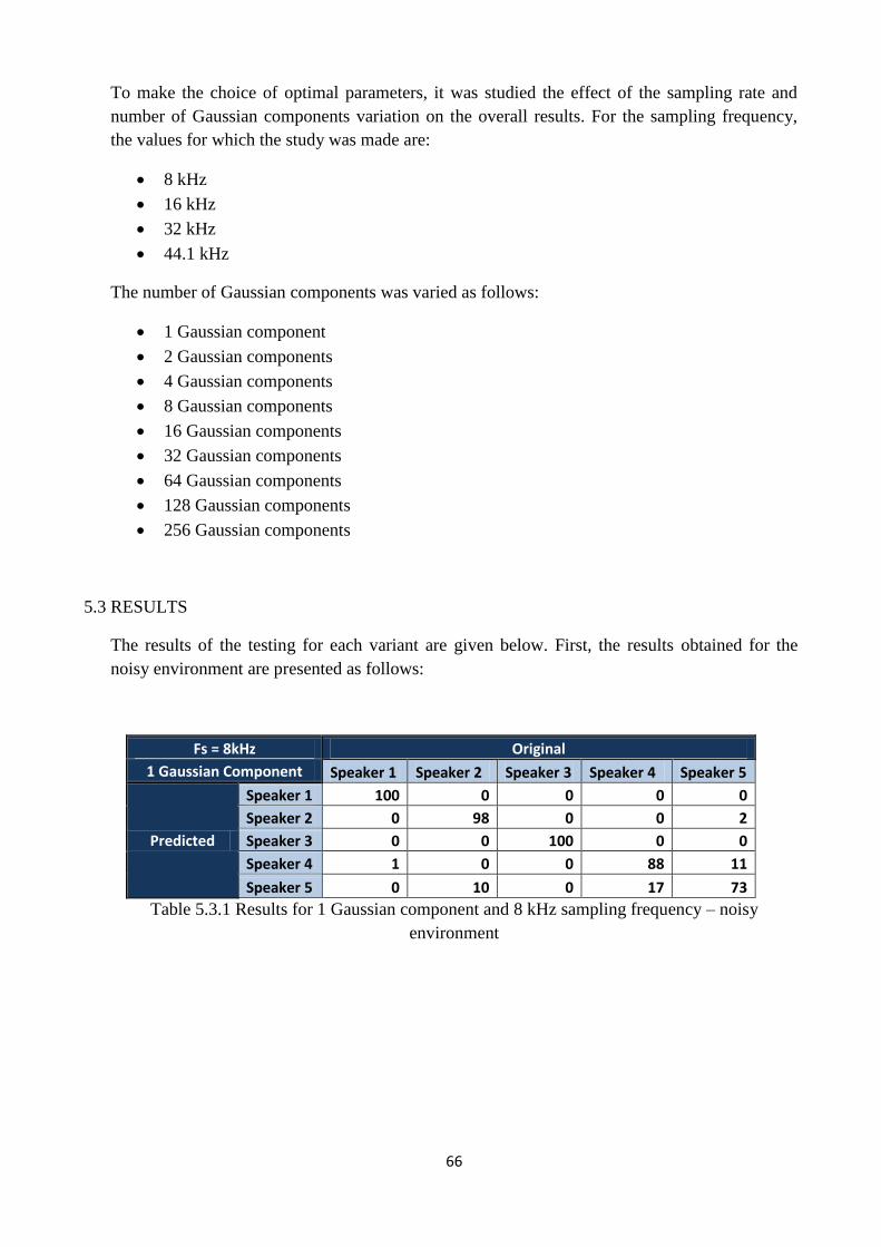
5.3 RESULTS

The results of the testing for each variant are given below. First, the results obtained for the

noisy environment are presented as follows:

Fs = 8kHz Original

1 Gaussian Component Speaker 1 Speaker 2 Speaker 3 Speaker 4 Speaker 5

Predicted

Speaker 1 100 0 0 0 0

Speaker 2 0 98 0 0 2

Speaker 3 0 0 100 0 0

Speaker 4 1 0 0 88 11

Speaker 5 0 10 0 17 73


environment

67

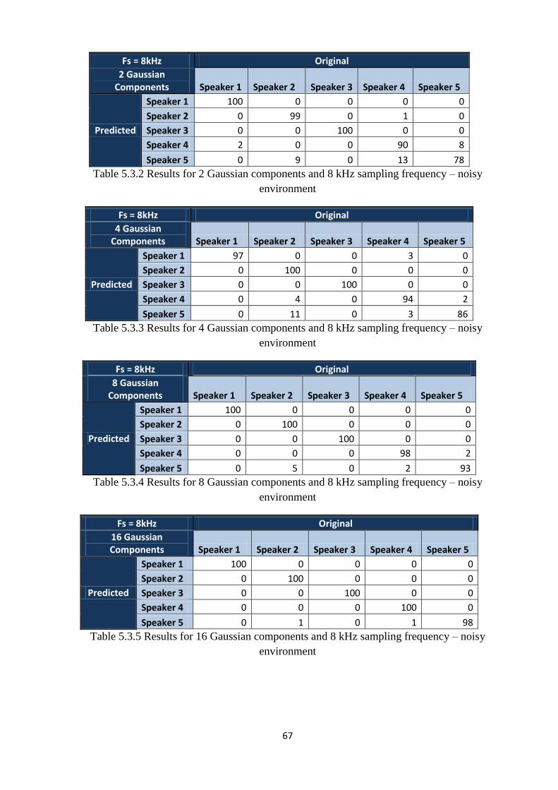
Fs = 8kHz Original

2 Gaussian Components Speaker 1 Speaker 2 Speaker 3 Speaker 4 Speaker 5

Predicted

Speaker 1 100 0 0 0 0

Speaker 2 0 99 0 1 0

Speaker 3 0 0 100 0 0

Speaker 4 2 0 0 90 8

Speaker 5 0 9 0 13 78


environment

Fs = 8kHz Original


Predicted

Speaker 1 97 0 0 3 0

Speaker 2 0 100 0 0 0

Speaker 3 0 0 100 0 0

Speaker 4 0 4 0 94 2

Speaker 5 0 11 0 3 86


environment

Fs = 8kHz Original


Predicted

Speaker 1 100 0 0 0 0

Speaker 2 0 100 0 0 0

Speaker 3 0 0 100 0 0

Speaker 4 0 0 0 98 2

Speaker 5 0 5 0 2 93


environment

Fs = 8kHz Original


Predicted

Speaker 1 100 0 0 0 0

Speaker 2 0 100 0 0 0

Speaker 3 0 0 100 0 0

Speaker 4 0 0 0 100 0

Speaker 5 0 1 0 1 98


environment

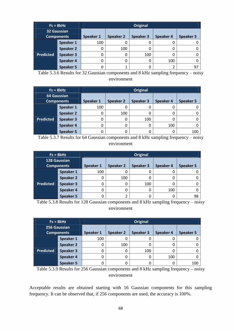
68

Fs = 8kHz Original


Predicted

Speaker 1 100 0 0 0 0

Speaker 2 0 100 0 0 0

Speaker 3 0 0 100 0 0

Speaker 4 0 0 0 100 0

Speaker 5 0 1 0 2 97


environment

Fs = 8kHz Original


Predicted

Speaker 1 100 0 0 0 0

Speaker 2 0 100 0 0 0

Speaker 3 0 0 100 0 0

Speaker 4 0 0 0 100 0

Speaker 5 0 0 0 0 100


environment

Fs = 8kHz Original


Predicted

Speaker 1 100 0 0 0 0

Speaker 2 0 100 0 0 0

Speaker 3 0 0 100 0 0

Speaker 4 0 0 0 100 0

Speaker 5 0 2 0 0 98


environment

Fs = 8kHz Original


Predicted

Speaker 1 100 0 0 0 0

Speaker 2 0 100 0 0 0

Speaker 3 0 0 100 0 0

Speaker 4 0 0 0 100 0

Speaker 5 0 0 0 0 100


environment

Acceptable results are obtained starting with 16 Gaussian components for this sampling

frequency. It can be observed that, if 256 components are used, the accuracy is 100%.

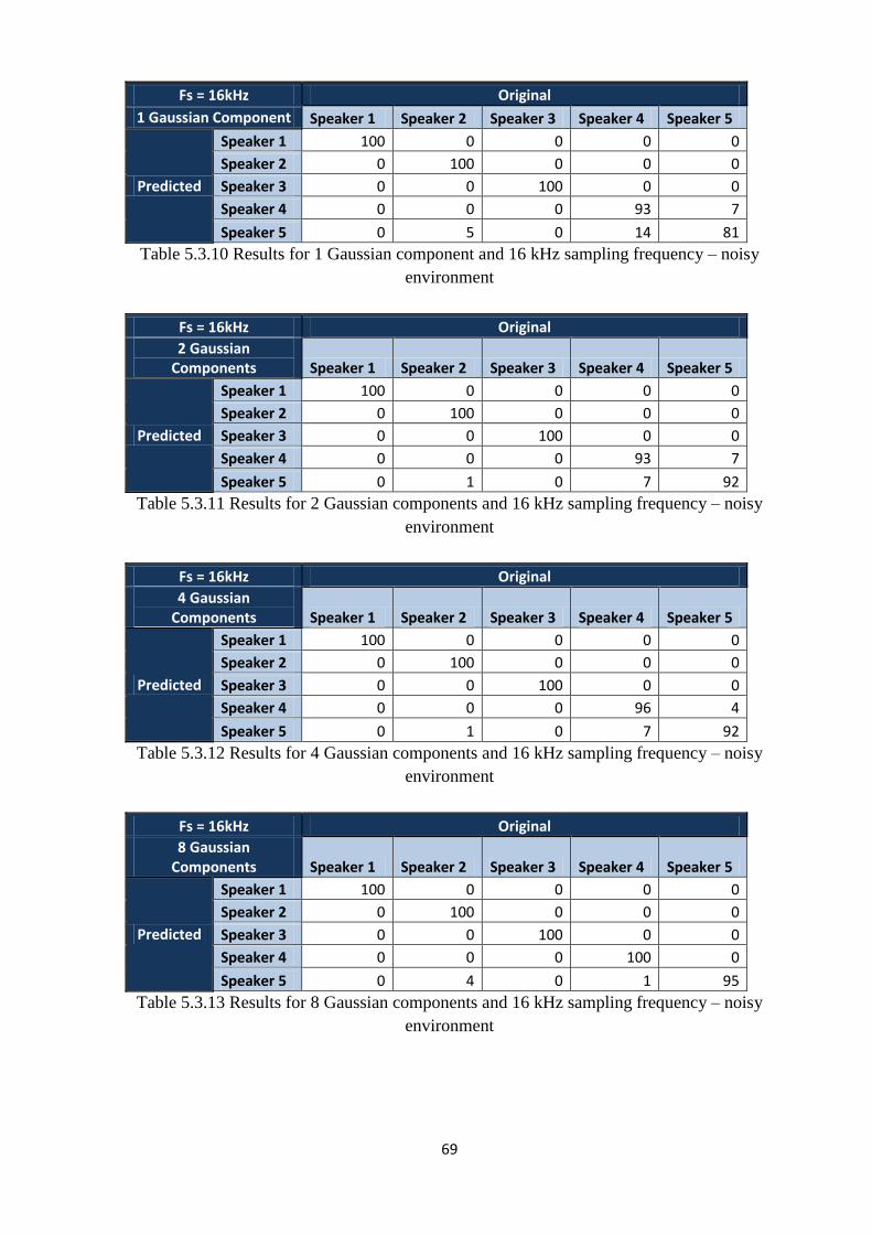
69

Fs = 16kHz Original


Predicted

Speaker 1 100 0 0 0 0

Speaker 2 0 100 0 0 0

Speaker 3 0 0 100 0 0

Speaker 4 0 0 0 93 7

Speaker 5 0 5 0 14 81


environment

Fs = 16kHz Original


Predicted

Speaker 1 100 0 0 0 0

Speaker 2 0 100 0 0 0

Speaker 3 0 0 100 0 0

Speaker 4 0 0 0 93 7

Speaker 5 0 1 0 7 92


environment

Fs = 16kHz Original


Predicted

Speaker 1 100 0 0 0 0

Speaker 2 0 100 0 0 0

Speaker 3 0 0 100 0 0

Speaker 4 0 0 0 96 4

Speaker 5 0 1 0 7 92


environment

Fs = 16kHz Original


Predicted

Speaker 1 100 0 0 0 0

Speaker 2 0 100 0 0 0

Speaker 3 0 0 100 0 0

Speaker 4 0 0 0 100 0

Speaker 5 0 4 0 1 95


environment

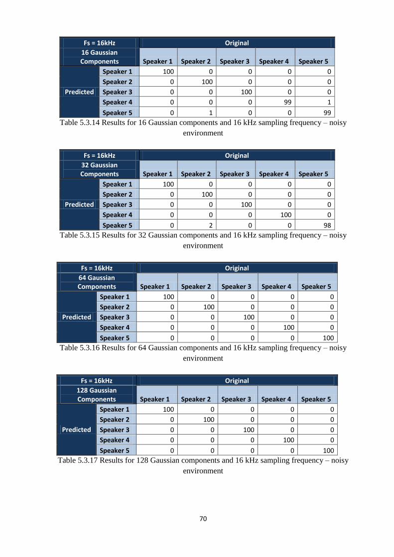
70

Fs = 16kHz Original


Predicted

Speaker 1 100 0 0 0 0

Speaker 2 0 100 0 0 0

Speaker 3 0 0 100 0 0

Speaker 4 0 0 0 99 1

Speaker 5 0 1 0 0 99


environment

Fs = 16kHz Original


Predicted

Speaker 1 100 0 0 0 0

Speaker 2 0 100 0 0 0

Speaker 3 0 0 100 0 0

Speaker 4 0 0 0 100 0

Speaker 5 0 2 0 0 98


environment

Fs = 16kHz Original


Predicted

Speaker 1 100 0 0 0 0

Speaker 2 0 100 0 0 0

Speaker 3 0 0 100 0 0

Speaker 4 0 0 0 100 0

Speaker 5 0 0 0 0 100


environment

Fs = 16kHz Original


Predicted

Speaker 1 100 0 0 0 0

Speaker 2 0 100 0 0 0

Speaker 3 0 0 100 0 0

Speaker 4 0 0 0 100 0

Speaker 5 0 0 0 0 100


environment

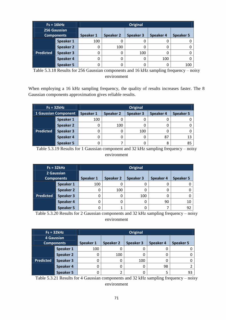
71

Fs = 16kHz Original


Predicted

Speaker 1 100 0 0 0 0

Speaker 2 0 100 0 0 0

Speaker 3 0 0 100 0 0

Speaker 4 0 0 0 100 0

Speaker 5 0 0 0 0 100


environment

When employing a 16 kHz sampling frequency, the quality of results increases faster. The 8

Gaussian components approximation gives reliable results.

Fs = 32kHz Original


Predicted

Speaker 1 100 0 0 0 0

Speaker 2 0 100 0 0 0

Speaker 3 0 0 100 0 0

Speaker 4 0 0 0 87 13

Speaker 5 0 7 0 8 85


environment

Fs = 32kHz Original


Predicted

Speaker 1 100 0 0 0 0

Speaker 2 0 100 0 0 0

Speaker 3 0 0 100 0 0

Speaker 4 0 0 0 90 10

Speaker 5 0 1 0 7 92


environment

Fs = 32kHz Original


Predicted

Speaker 1 100 0 0 0 0

Speaker 2 0 100 0 0 0

Speaker 3 0 0 100 0 0

Speaker 4 0 0 0 98 2

Speaker 5 0 2 0 5 93


environment

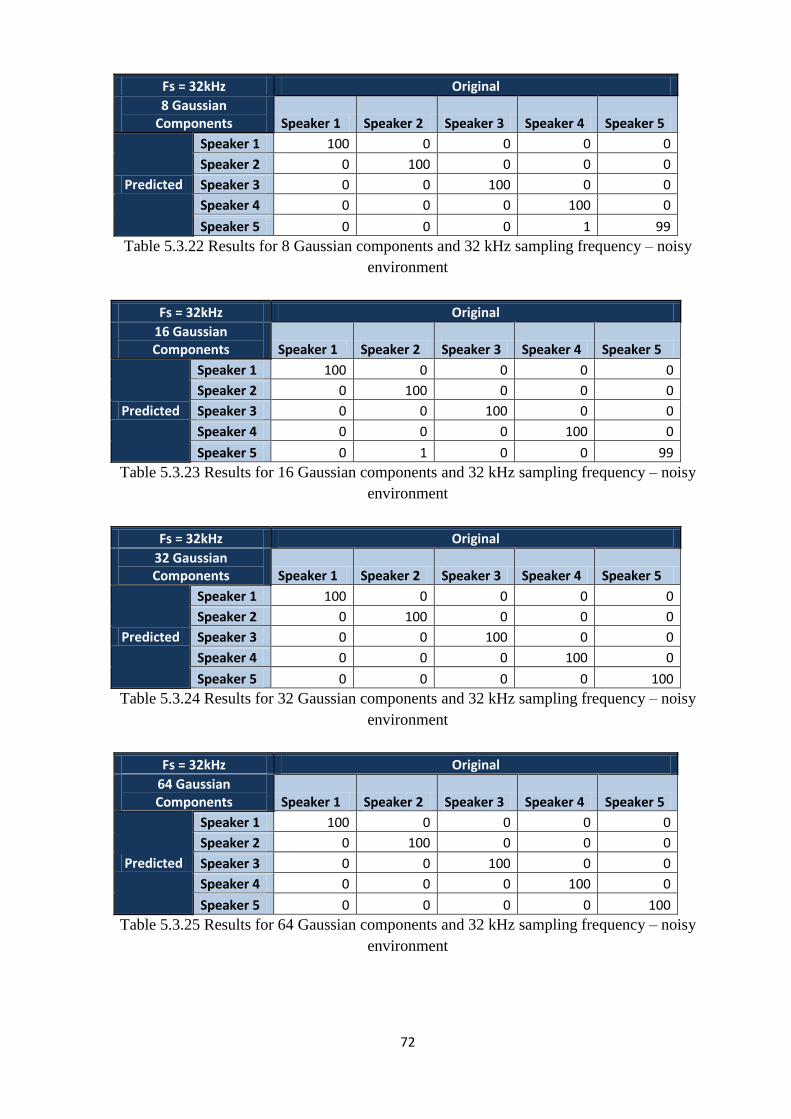
72

Fs = 32kHz Original


Predicted

Speaker 1 100 0 0 0 0

Speaker 2 0 100 0 0 0

Speaker 3 0 0 100 0 0

Speaker 4 0 0 0 100 0

Speaker 5 0 0 0 1 99


environment

Fs = 32kHz Original


Predicted

Speaker 1 100 0 0 0 0

Speaker 2 0 100 0 0 0

Speaker 3 0 0 100 0 0

Speaker 4 0 0 0 100 0

Speaker 5 0 1 0 0 99


environment

Fs = 32kHz Original


Predicted

Speaker 1 100 0 0 0 0

Speaker 2 0 100 0 0 0

Speaker 3 0 0 100 0 0

Speaker 4 0 0 0 100 0

Speaker 5 0 0 0 0 100


environment

Fs = 32kHz Original


Predicted

Speaker 1 100 0 0 0 0

Speaker 2 0 100 0 0 0

Speaker 3 0 0 100 0 0

Speaker 4 0 0 0 100 0

Speaker 5 0 0 0 0 100


environment

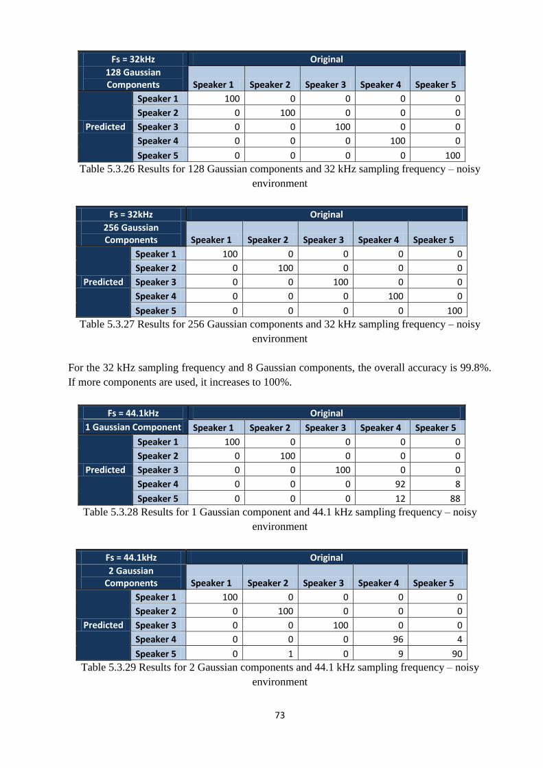
73

Fs = 32kHz Original


Predicted

Speaker 1 100 0 0 0 0

Speaker 2 0 100 0 0 0

Speaker 3 0 0 100 0 0

Speaker 4 0 0 0 100 0

Speaker 5 0 0 0 0 100


environment

Fs = 32kHz Original


Predicted

Speaker 1 100 0 0 0 0

Speaker 2 0 100 0 0 0

Speaker 3 0 0 100 0 0

Speaker 4 0 0 0 100 0

Speaker 5 0 0 0 0 100


environment

For the 32 kHz sampling frequency and 8 Gaussian components, the overall accuracy is 99.8%.

If more components are used, it increases to 100%.

Fs = 44.1kHz Original


Predicted

Speaker 1 100 0 0 0 0

Speaker 2 0 100 0 0 0

Speaker 3 0 0 100 0 0

Speaker 4 0 0 0 92 8

Speaker 5 0 0 0 12 88

Table 5.3.28 Results for 1 Gaussian component and 44.1 kHz sampling frequency – noisy

environment



Predicted

Speaker 1 100 0 0 0 0

Speaker 2 0 100 0 0 0

Speaker 3 0 0 100 0 0

Speaker 4 0 0 0 96 4

Speaker 5 0 1 0 9 90


environment

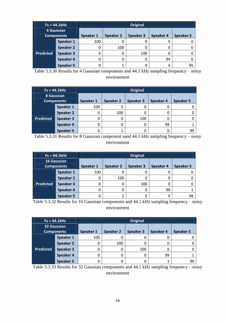
74



Predicted

Speaker 1 100 0 0 0 0

Speaker 2 0 100 0 0 0

Speaker 3 0 0 100 0 0

Speaker 4 0 0 0 94 6

Speaker 5 0 1 0 4 95


environment



Predicted

Speaker 1 100 0 0 0 0

Speaker 2 0 100 0 0 0

Speaker 3 0 0 100 0 0

Speaker 4 0 0 0 99 1

Speaker 5 0 1 0 0 99

Table 5.3.31 Results for 8 Gaussian component sand 44.1 kHz sampling frequency – noisy

environment



Predicted

Speaker 1 100 0 0 0 0

Speaker 2 0 100 0 0 0

Speaker 3 0 0 100 0 0

Speaker 4 0 0 0 99 1

Speaker 5 0 2 0 0 98


environment



Predicted

Speaker 1 100 0 0 0 0

Speaker 2 0 100 0 0 0

Speaker 3 0 0 100 0 0

Speaker 4 0 0 0 99 1

Speaker 5 0 0 0 1 99


environment

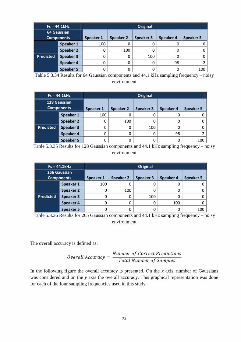
75



Predicted

Speaker 1 100 0 0 0 0

Speaker 2 0 100 0 0 0

Speaker 3 0 0 100 0 0

Speaker 4 0 0 0 98 2

Speaker 5 0 0 0 0 100


environment



Predicted

Speaker 1 100 0 0 0 0

Speaker 2 0 100 0 0 0

Speaker 3 0 0 100 0 0

Speaker 4 0 0 0 98 2

Speaker 5 0 0 0 0 100


environment



Predicted

Speaker 1 100 0 0 0 0

Speaker 2 0 100 0 0 0

Speaker 3 0 0 100 0 0

Speaker 4 0 0 0 100 0

Speaker 5 0 0 0 0 100


environment

The overall accuracy is defined as:

In the following figure the overall accuracy is presented. On the x axis, number of Gaussians

was considered and on the y axis the overall accuracy. This graphical representation was done

for each of the four sampling frequencies used in this study.

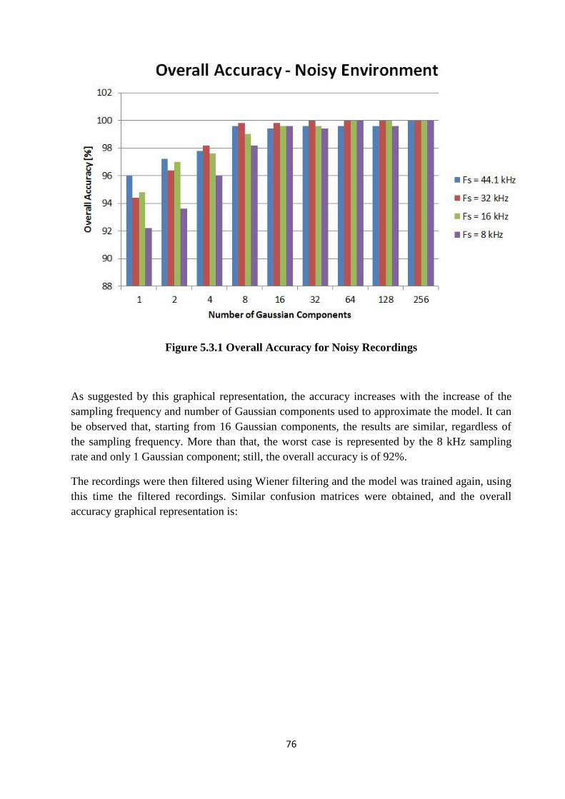
76

Figure 5.3.1 Overall Accuracy for Noisy Recordings

As suggested by this graphical representation, the accuracy increases with the increase of the

sampling frequency and number of Gaussian components used to approximate the model. It can

be observed that, starting from 16 Gaussian components, the results are similar, regardless of

the sampling frequency. More than that, the worst case is represented by the 8 kHz sampling

rate and only 1 Gaussian component; still, the overall accuracy is of 92%.

The recordings were then filtered using Wiener filtering and the model was trained again, using

this time the filtered recordings. Similar confusion matrices were obtained, and the overall

accuracy graphical representation is:

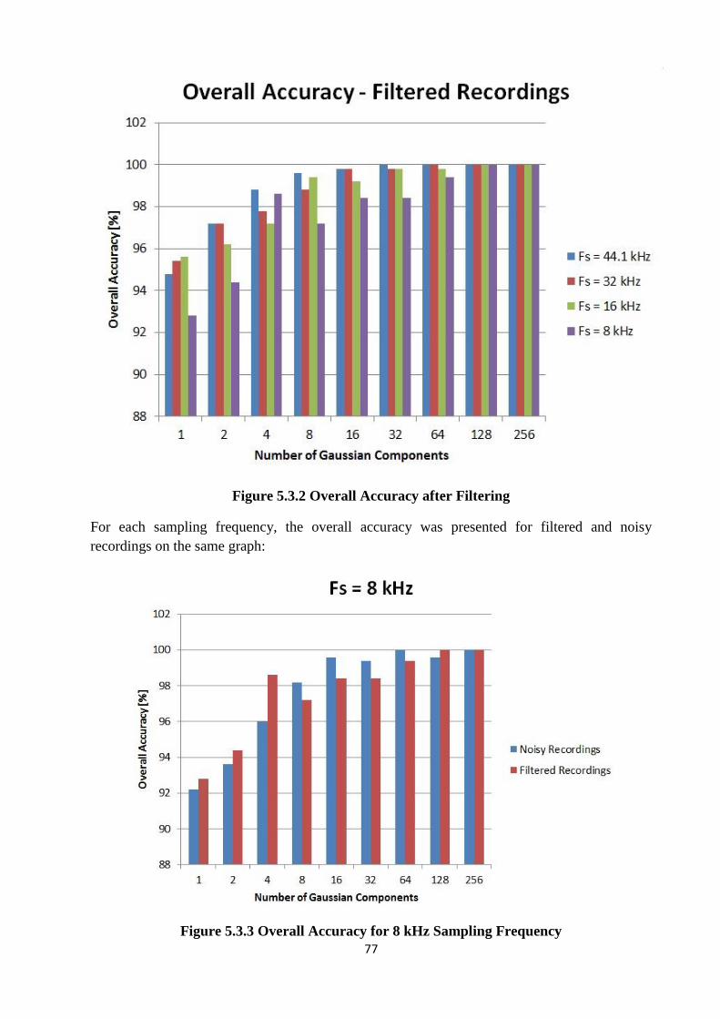
77

Figure 5.3.2 Overall Accuracy after Filtering

For each sampling frequency, the overall accuracy was presented for filtered and noisy

recordings on the same graph:

Figure 5.3.3 Overall Accuracy for 8 kHz Sampling Frequency

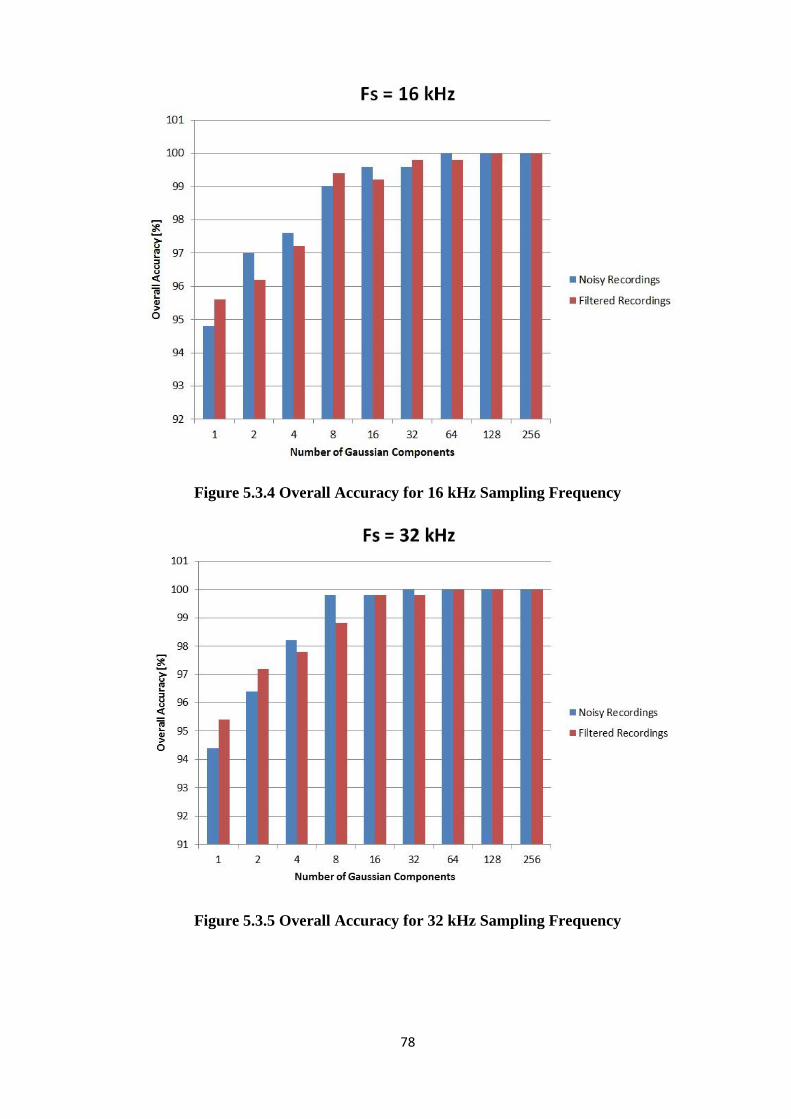
78



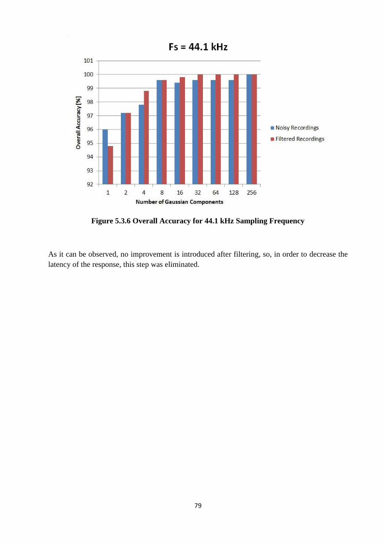
79

Figure 5.3.6 Overall Accuracy for 44.1 kHz Sampling Frequency

As it can be observed, no improvement is introduced after filtering, so, in order to decrease the

latency of the response, this step was eliminated.

81

CHAPTER 6

CONCLUSION

The main objective of this thesis was to develop a system that recognizes the speaker from a small

speaker’s set. The project could be divided into three major sections: data acquisition, training and

testing.

As stated in the introduction, the purpose of such an approach is to help increase the autonomy of

the NAO robot, such that it can interact easily with children. The thesis is desired to be part of a

much ampler project that has as goal the introduction in therapy of the robot. This idea is sustained

by intensive studies that seem to indicate an increased efficiency in children’s therapy when using

such a robot. The voice recognition project was developed as it is desired to have a mean of

identifying the patients, in order to keep track of their performance. Since the number of children

that are part of the study is limited the speaker’s set is initially of only 5 speakers; more will be

added if and when necessary. More than that, most of the responses to tasks employed in therapy

sessions are based on a given script, so the method used is text dependent.

Some of the most important conclusions that could be drawn from this study are:

The method is noise robust. Indeed, as it was previously proven, the results are similar for

noisy and filtered recordings.

A compromise between the complexity of the algorithm and the results should be made. The

best results are obtained for the highest sampling frequency and the largest number of

Gaussian components. But these values (44.1 kHz sampling frequency and 256 Gaussian

components) increase not only the memory occupied, but also the response time. Still, very

good results are obtained for some lower values for these two parameters.

The worst case scenario is obtained for a sampling frequency of 8 kHz and only 1 Gaussian

component, as it was expected. As observed from the graphical representation previously

given, the overall accuracy is still greater than 92%. An explanation for this good result is

the low number of speakers, together with the low number of voice commands.

82

Another important conclusion that can be drawn is that, for 16 Gaussian components or

more, the results in terms of the overall accuracy are similar, regardless of the sampling

frequency. Based on this observation, the number of Gaussian components could be

decreased, which in turn will lead to a decrease in the response time.

As it was proven by the values from the confusion matrices presented in the previous

chapter, the most mix-ups appear between speaker 4 and speaker 5. Both speakers were

female and the most probable explanation for this phenomenon is represented by the

similitudes in their voice characteristics.

The personal contributions to this project are:

The recording of voice commands

The database creation

The model training

The study of the effect of varying sampling frequency and number of Gaussian components

The study of the effect of filtering on the overall accuracy

The implementation of the program on the robot

With the technology rapidly evolving, such a project needs to keep up. Some future improvements

could be made, especially in the latency decrease direction. Also, if needed, the database could be

increased by increasing the number of speakers.

Another aspect that would be an important step towards the autonomy of the robot is the voice

activity detection that, if implemented on NAO, would allow it to start acquiring data without any

external interference.

83

REFERENCES

[1] Humanoid Robot, https://www.sciencedaily.com/terms/humanoid_robot.htm (accessed on

March-12-2018)

[2] Pfeiffer R. Scheier C. “Understanding Intelligence” Bradford Books 2 11

[3] Humanoid robots, learning tools in the world of education,

https://www.ald.softbankrobotics.com/en/solutions/education-research (accessed on March-12-

2018)

[4] NAO, https://jgrcommunications.com/wp-content/uploads/2016/03/Nao.jpg (accessed on March-

12-2018)

[5] SoftBank Robotics Documentation, http://doc.aldebaran.com/2-1/home_nao (accessed on

March-12-2018)

[6] LED’s position on NAO robot, http://www.cs.cmu.edu/~cga/nao/doc/reference-

documentation/naoqi/sensors/alleds.html (accessed on March-15-2018)

[7] Wiener filter, https://en.wikipedia.org/wiki/Wiener_filter (accessed on May-12-2108)

[8] Shimkin, N., “Estimation and Identification in Dynamical System”, Lecture Notes, fall 2009,

Israel Institute of Technology, Department of Electrical Engineering

[9] Dobre, R., “Multimedia Coding-Techniques and Applications”, Lecture Notes, 2018, Faculty of

Electronics, Telecommunications and Information Technology

[10] Signal Processing, https://dsp.stackexchange.com (accessed on May-12-2018)

[11] Jurafsky, D., Martin, J.H. “Speech and Language Processing” Pearson Education Limited,

2014, p.176-181, 188-194, 298-308, 312-318

[12] Hidden Markov Models, https://www.lrde.epita.fr/~reda/cours/speech/PH%20

Spoken%20Language%20Processing%20%20A%20Guide%20to%20Theory,%20Algorithm%20an

d%20System%20Development%20(2001)/chapter8.pdf (accessed on May-12-2018)

[13] Martin, J. “Natural Language Processing” Lecture 8 9-24-2013

[14] What is a phone, https://glossary.sil.org/term/phone (accessed on June-02-2018)

[15] Recognition System of Japanese Characters,

http://www.takanishi.mech.waseda.ac.jp/top/solis/Recognition_Systems/recognition.html (accessed

on June-02-2018)

[16] Jurafsky, D., “Spoken Language Processing” Stanford University spring 2 14

https://www.sciencedaily.com/terms/humanoid_robot.htm

https://www.ald.softbankrobotics.com/en/solutions/education-research

https://jgrcommunications.com/wp-content/uploads/2016/03/Nao.jpg

http://doc.aldebaran.com/2-1/home_nao

http://www.cs.cmu.edu/~cga/nao/doc/reference-documentation/naoqi/sensors/alleds.html

http://www.cs.cmu.edu/~cga/nao/doc/reference-documentation/naoqi/sensors/alleds.html

https://en.wikipedia.org/wiki/Wiener_filter

https://dsp.stackexchange.com/

https://www.lrde.epita.fr/~reda/cours/speech/PH%20%20Spoken%20Language%20Processing%20%20A%20Guide%20to%20Theory,%20Algorithm%20and%20System%20Development%20(2001)/chapter8.pdf



https://glossary.sil.org/term/phone

http://www.takanishi.mech.waseda.ac.jp/top/solis/Recognition_Systems/recognition.html

84

[17] Jurafsky, D. “Automatic Speech Recognition” Stanford University spring 2 14

[18] Filtering a sound recording, https://rsmith.home.xs4all.nl/miscellaneous/filtering-a-sound-

recording.html (accessed on June-04-2018)

[19] Fayek, H. “Speech Processing for Machine Learning: Filter banks, Mel-Frequency Cepsral

Coefficients (MFCCs) and What’s in Between” April-21-2016

[20] Distributions of One Variable, http://work.thaslwanter.at/Stats/html/statsDistributions.html

(accessed on June-05-2018)

[21] Lee, Jin Long “Anomaly Detection, part 2: Multivariate Gaussian Distribution” Study Notes

June-30-2015

[22] Bhattacharjee, U., Sarmah, K. “GMM-UBM Based Speaker Verification in Multilingual

Environments”, IJCSI International Journal of Computer Science Issues, volume 9, issue 6, no 2,

November 2012

[23] Karpov, E. “Efficient Speaker Recognition for Mobile Devices” Publications of the University

of Eastern Finland Dissertations in Forestry and Natural Sciences, November 2011

[24] Reynolds, D.A., Rose, R.C. “Robust Text-Independent Speaker Identification Using Gaussian

Mixture Speakers Models” IEEE Transactions on Speech and Audio Processing volume 3 no 1

January 1995

[25] Gaussian Mixture Models, https://prateekvjoshi.com/2013/06/29/gaussian-mixture-models/

(accessed on June-06-2018)

[26] Reynolds, D.A., Quatieri, T.F., Dunn, R.B. “Speaker Verification Using Adapted Gaussian

Mixture Models” Digital Signal Processing volume 1 no 1-3, January/April/July 2000

[27] Vuuren S. “Speaker Verification in a Time-Feature Space” Ph.D. thesis Oregon Graduate

Institute, March 1999

https://rsmith.home.xs4all.nl/miscellaneous/filtering-a-sound-recording.html

https://rsmith.home.xs4all.nl/miscellaneous/filtering-a-sound-recording.html

http://work.thaslwanter.at/Stats/html/statsDistributions.html

https://prateekvjoshi.com/2013/06/29/gaussian-mixture-models/

diploma thesis - speed · bucharest 2018 university “politehnica” of bucharest faculty of...

Documents