dirac operators and spectral triples for some fractal sets built on curves
TRANSCRIPT
Advances in Mathematics 217 (2008) 42–78www.elsevier.com/locate/aim
Dirac operators and spectral triples for some fractal setsbuilt on curves
Erik Christensen a,∗, Cristina Ivan b, Michel L. Lapidus c,1
a Department of Mathematics, University of Copenhagen, DK-2100 Copenhagen, Denmarkb Department of Mathematics, University of Hannover, 30167 Hannover, Germany
c Department of Mathematics, University of California, Riverside, CA 92521-0135, USA
Received 10 October 2006; accepted 14 June 2007
Available online 27 June 2007
Communicated by Michael J. Hopkins
Abstract
We construct spectral triples and, in particular, Dirac operators, for the algebra of continuous functionson certain compact metric spaces. The triples are countable sums of triples where each summand is basedon a curve in the space. Several fractals, like a finitely summable infinite tree and the Sierpinski gasket, fitnaturally within our framework. In these cases, we show that our spectral triples do describe the geodesicdistance and the Minkowski dimension as well as, more generally, the complex fractal dimensions of thespace. Furthermore, in the case of the Sierpinski gasket, the associated Dixmier-type trace coincides withthe normalized Hausdorff measure of dimension log 3/ log 2.© 2007 Elsevier Inc. All rights reserved.
MSC: primary 28A80, 46L87; secondary 53C22, 58B34
Keywords: Compact and Hausdorff spaces; Dirac operators; Spectral triples; C*-algebras; Noncommutative geometry;Parameterized graphs; Fractals; Finitely summable trees; Cayley graphs; Sierpinski gasket; Metric; Minkowski andHausdorff dimensions; Complex fractal dimensions; Dixmier trace; Hausdorff measure; Geodesic metric; Analysison fractals
* Corresponding author.E-mail addresses: [email protected] (E. Christensen), [email protected] (C. Ivan),
[email protected] (M.L. Lapidus).1 The work of the author was partially supported by the US National Science Foundation under the research grants
DMS-0070497 and DMS-0707524.
0001-8708/$ – see front matter © 2007 Elsevier Inc. All rights reserved.doi:10.1016/j.aim.2007.06.009

E. Christensen et al. / Advances in Mathematics 217 (2008) 42–78 43
0. Introduction
Consider a smooth compact spin Riemannian manifold M and the Dirac operator ∂M associ-ated with a fixed Riemannian connexion over the spinor bundle S. Let D denote the extension of∂M to H , the Hilbert space of square-integrable sections (or spinors) of S. Then Alain Connesshowed that the geodesic distance, the dimension of M and the Riemannian volume measurecan all be described via the operator D and its associated Dixmier trace. This observation makesit possible to reformulate the geometry of a manifold in terms of a representation of the alge-bra of continuous functions as operators on a Hilbert space on which an unbounded self-adjointoperator D acts. The geometric structures are thus described in such a way that points in themanifold are not mentioned at all. It is then possible to replace the commutative algebra of coor-dinates by a not necessarily commutative algebra, and a way of expressing geometric propertiesfor noncommutative algebras has been opened.
Connes, alone or in collaborations, has extensively developed the foregoing idea. (See, forexample, the paper [5], the book [6] and the recent survey article [8], along with the relevantreferences therein.) He has shown how an unbounded Fredholm module over the algebra A ofcoordinates of a possibly noncommutative space X specifies some elements of the (quantized)differential and integral calculus on X as well as the metric structure of X. An unbounded Fred-holm module (H,D) consists of a representation of A as bounded operators on a Hilbert spaceH and an unbounded self-adjoint operator D on H satisfying certain axioms. This operator isthen called a Dirac operator and, if the representation is faithful, the triple (A,H,D) is called aspectral triple.
The introduction of the concept of a spectral triple for a not necessarily commutative algebraA makes it possible to assign a subalgebra of A as playing the role of the algebra of the infinitelydifferentiable functions, even though expressions of the type (f (x)−f (y))/(x −y) do not makesense anymore.
With this space-free description of some elements of differential geometry at our disposal,a new way of investigating the geometry of fractal sets seems to be possible. Fractal sets arenonsmooth in the traditional sense, so at first it seems quite unreasonable to try to apply themethods of differential geometry in the study of such sets. On the other hand, any compact setT is completely described as the spectrum of the C*-algebra C(T ) consisting of the continuouscomplex functions on it. This means that if we can apply Connes’ space-free techniques to adense subalgebra of C(T ), then we do get some insight into the sort of geometric structures onthe compact space T that are compatible with the given topology.
Already, in their unpublished work [9], Alain Connes and Dennis Sullivan have developeda ‘quantized calculus’ on the limit sets of ‘quasi-Fuchsian’ groups, including certain Julia sets.Their results are presented in [6, Chapter 4, Sections 3.γ and 3.ε], along with related results ofConnes on Cantor-type sets (see also [7]). The latter are motivated in part by the work of MichelLapidus and Carl Pomerance [32] or Helmut Maier [31] on the geometry and spectra of fractalstrings and their associated zeta functions (now much further expanded in the theory of ‘complexfractal dimensions’ developed in the books [29,30]).
In particular, in certain cases, the Minkowski dimension and the Hausdorff measure can berecovered from operator algebraic data. Work in this direction was pursued by Daniele Guidoand Tommaso Isola in several papers, [16–18].
Earlier, in [27], using the results and methods of [21] and [6] (including the notion of ‘Dixmiertrace’), Lapidus has constructed an analogue of (Riemannian) volume measures on finitely ram-ified or p.c.f. self-similar fractals and related them to the notion of ‘spectral dimension,’ which

44 E. Christensen et al. / Advances in Mathematics 217 (2008) 42–78
gives the asymptotic growth rate of the spectra of Laplacians on these fractals. (See also [22]where these volume measures were later precisely identified, for a class of fractals including theSierpinski gasket.) In his programmatic paper [28], building upon [27], he then investigated inmany different ways the possibility of developing a kind of noncommutative fractal geometry,which would merge aspects of analysis on fractals (as now presented e.g. in [20]) and Connes’noncommutative geometry [6]. (See also parts of [26] and [27].) Central to [28] was the proposalto construct suitable spectral triples that would capture the geometric and spectral aspects of agiven self-similar fractal, including its metric structure. Much remains to be done in this direc-tion, however, but the present work, along with some of its predecessors mentioned above andbelow, address these issues from a purely geometric point of view. In later work, we hope to beable to extend our construction to address some of the more spectral aspects.
In [2], Erik Christensen and Cristina Ivan constructed a spectral triple for the approximatelyfinite-dimensional (AF) C*-algebras. The continuous functions on the Cantor set form an AFC*-algebra since the Cantor set is totally disconnected. Hence, it was quite natural to try toapply the general results of that paper for AF C*-algebras to this well-known example. In thismanner, they showed in [2] once again how suitable noncommutative geometry may be to thestudy of the geometry of a fractal. Since then, the authors of the present article have searchedfor possible spectral triples associated to other known fractals. The hope is that these triples maybe relevant to both fractal geometry and analysis on fractals. We have been especially interestedin the Sierpinski gasket, a well-known nowhere differentiable planar curve, because of its keyrole in the development of harmonic analysis on fractals. (See, for example, [1,20,39,40].) Wepresent here a spectral triple for this fractal which recovers its geometry very well. In particular,it captures some of the visually detectable aspects of the gasket.
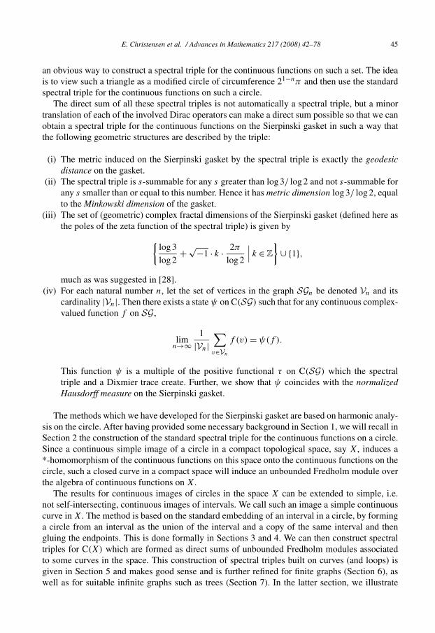
We will now give a more detailed description of the Sierpinski gasket and of the spectral triplewe construct in that case. The way of looking at the gasket, upon which our construction is based,is as the closure of the limit of an increasing sequence of graphs. The pictures in Fig. 1 illustratethis. We have chosen the starting approximation, SG0, as a triangle, and as a graph it consists of3 vertices and 3 edges. The construction is of course independent of the scale, but we will assumethat we work in the Euclidean plane and that the usual concept of length is given. We then fixthe size of the largest triangle such that all the sides have length 2π/3. Then, for any naturalnumber n, the nth approximation SGn is constructed from SGn−1 by adding 3n new verticesand 3n new edges of length 21−nπ/3. It is possible to construct a spectral triple for the gasketby constructing a spectral triple for each new edge introduced in one of the graphs SGn, but inorder to let the spectral triples describe the holes too, and not only the lines, we have chosento look at this iterative construction as an increasing union of triangles. Hence, SG0 consists ofone equilateral triangle with circumference (i.e., perimeter) equal to 2π and SG1 consists of theunion of 3 equilateral triangles each of circumference π . Continuing in this manner, we get forany natural number n that SGn is a union of 3n equilateral triangles of side length 21−nπ/3. Theadvantage of this description is that, for any equilateral triangle of circumference 21−nπ , there is
Fig. 1. The first 3 pre-fractal approximations to the Sierpinski gasket.
E. Christensen et al. / Advances in Mathematics 217 (2008) 42–78 45
an obvious way to construct a spectral triple for the continuous functions on such a set. The ideais to view such a triangle as a modified circle of circumference 21−nπ and then use the standardspectral triple for the continuous functions on such a circle.
The direct sum of all these spectral triples is not automatically a spectral triple, but a minortranslation of each of the involved Dirac operators can make a direct sum possible so that we canobtain a spectral triple for the continuous functions on the Sierpinski gasket in such a way thatthe following geometric structures are described by the triple:
(i) The metric induced on the Sierpinski gasket by the spectral triple is exactly the geodesicdistance on the gasket.
(ii) The spectral triple is s-summable for any s greater than log 3/ log 2 and not s-summable forany s smaller than or equal to this number. Hence it has metric dimension log 3/ log 2, equalto the Minkowski dimension of the gasket.
(iii) The set of (geometric) complex fractal dimensions of the Sierpinski gasket (defined here asthe poles of the zeta function of the spectral triple) is given by
{log 3
log 2+ √−1 · k · 2π
log 2
∣∣∣ k ∈ Z
}∪ {1},
much as was suggested in [28].(iv) For each natural number n, let the set of vertices in the graph SGn be denoted Vn and its
cardinality |Vn|. Then there exists a state ψ on C(SG) such that for any continuous complex-valued function f on SG,
limn→∞
1
|Vn|∑v∈Vn
f (v) = ψ(f ).
This function ψ is a multiple of the positive functional τ on C(SG) which the spectraltriple and a Dixmier trace create. Further, we show that ψ coincides with the normalizedHausdorff measure on the Sierpinski gasket.
The methods which we have developed for the Sierpinski gasket are based on harmonic analy-sis on the circle. After having provided some necessary background in Section 1, we will recall inSection 2 the construction of the standard spectral triple for the continuous functions on a circle.Since a continuous simple image of a circle in a compact topological space, say X, induces a*-homomorphism of the continuous functions on this space onto the continuous functions on thecircle, such a closed curve in a compact space will induce an unbounded Fredholm module overthe algebra of continuous functions on X.
The results for continuous images of circles in the space X can be extended to simple, i.e.not self-intersecting, continuous images of intervals. We call such an image a simple continuouscurve in X. The method is based on the standard embedding of an interval in a circle, by forminga circle from an interval as the union of the interval and a copy of the same interval and thengluing the endpoints. This is done formally in Sections 3 and 4. We can then construct spectraltriples for C(X) which are formed as direct sums of unbounded Fredholm modules associatedto some curves in the space. This construction of spectral triples built on curves (and loops) isgiven in Section 5 and makes good sense and is further refined for finite graphs (Section 6), aswell as for suitable infinite graphs such as trees (Section 7). In the latter section, we illustrate
46 E. Christensen et al. / Advances in Mathematics 217 (2008) 42–78
our results by considering the fractal tree (Cayley graph) associated to F2, the noncommutativefree group of two generators. In Section 8, we then apply our results and study in detail theirconsequences for the important example of the Sierpinski gasket, as described above. Finally, inSection 9, we close this paper by discussing several open problems and proposing directions forfurther research.
1. Notation and preliminaries
In the book [6], Connes explains how a lot of geometric properties of a compact space X canbe described via the algebra of continuous functions C(X), representations of this algebra andsome unbounded operators on a Hilbert space like differential operators. The concepts mentioneddo not rely on the commutativity of the algebra C(X), so it is possible to consider a general non-commutative C*-algebra, its representations and some unbounded operators on a Hilbert spaceas noncommutative versions of structures which in the first place have been expressed in terms ofsets and geometric properties. In particular, the closely related notions of unbounded Fredholmmodule and spectral triple are fundamental and we will recall them here.
Definition 1.1. Let A be a unital C*-algebra. An unbounded Fredholm module (H,D) over Aconsists of a Hilbert space H which carries a unital representation π of A and an unbounded,self-adjoint operator D on H such that
(i) the set {a ∈ A | [D,π(a)] is densely defined and extends to a bounded operator on H } is adense subset of A,
(ii) the operator (I + D2)−1 is compact.
If, in addition, tr((I + D2)−p/2) < ∞ for some positive real number p, then the unboundedFredholm module, is said to be p-summable, or just finitely summable. The number dST given by
dST := inf{p > 0
∣∣ tr((
I + D2)−p/2)< ∞}
is called the metric dimension of the unbounded Fredholm module.
Definition 1.2. Let A be a unital C*-algebra and (H,D) an unbounded Fredholm module over A.If the underlying representation π is faithful, then (A,H,D) is called a spectral triple.
For notational simplicity, we will denote by (A,H,D) either a spectral triple or an unboundedFredholm module, whether or not the underlying representation is faithful.
We will refer to Connes’ book [6] on several occasions later in this article. As a standardreference on the theory of operator algebras, we use the books by Kadison and Ringrose [19].
The emphasis of this article is actually not very much on noncommutative C*-algebras andnoncommutative geometry, but our interest here is to see to what extend the spectral triples(unbounded Fredholm modules) of noncommutative geometry can be used to describe compactspaces of a fractal nature. In the papers [2,3], one can find investigations of this sort for theCantor set and for general compact metric spaces, respectively. The metrics of compact spacesintroduced via noncommutative geometric methods were extensively investigated by Marc Rief-fel. (See, for example, the papers [34–37].)

E. Christensen et al. / Advances in Mathematics 217 (2008) 42–78 47
Our standard references for concepts from fractal geometry are Edgar’s books [12,13], Fal-coner’s book [15] and Lapidus and Frankenhuijsen’s books [29,30].
2. The spectral triple for a circle
Much of the material in this section is well known (see e.g. [14]) but is not traditionallypresented in the language of spectral triples. It is useful, however, to discuss it here becauseto our knowledge, it is only available in scattered references and not in the form we need it.In particular, we will study in some detail the domains of definition of the relevant unboundedoperators and derivations.
Let Cr denote the circle in the complex plane with radius r > 0 and centered at 0. As usualin noncommutative geometry, we are not studying the circle directly but rather a subalgebra ofthe algebra of continuous functions on it. From this point of view, it seems easier to look at thealgebra of complex continuous 2πr-periodic functions on the real line. We will let ACr denotethis algebra. We will let (1/2πr)m denote the normalized Lebesgue measure on the interval[−πr,πr] and let πr be the standard representation of ACr as multiplication operators on theHilbert space Hr which is defined by Hr := L2([−πr,πr], (1/2πr)m). The space Hr has acanonical orthonormal basis, denoted (φr
k)k∈Z, which consists of functions in ACr given by
∀k ∈ Z, φrk(x) := exp
(ikx
r
).
These functions are eigenfunctions of the differential operator 1i
ddx
and the corresponding eigen-values are {k/r | k ∈ Z}. The natural choice for the Dirac operator for this situation is the closureof the restriction of the above operator to the linear span of the basis {φr
k | k ∈ Z}. We will let Dr
denote this operator on Hr . It is well known that Dr is self-adjoint and that dom(Dr), the domainof definition of Dr , is given by
∀f ∈ Hr : f ∈ domDr ⇔∑k∈Z
k2
r2
∣∣⟨f ∣∣ φrk
⟩∣∣2< ∞,
where 〈· | ·〉 is the inner product of Hr .For an element f ∈ domDr , we have Drf = ∑
k∈Z(k/r)〈f | φr
k〉φrk . The self-adjoint operator
Dr has spectrum {k/r | k ∈ Z} and each of its eigenvalues has multiplicity 1. Furthermore, anycontinuously differentiable 2πr-periodic function f on R satisfies
[Dr,πr(f )
] = πr
(−if ′),so we obtain a spectral triple associated to the circle Cr in the following manner.
Definition 2.1. The natural spectral triple, STn(Cr), for the circle algebra ACr is defined bySTn(Cr) := (ACr,Hr,Dr).
One of the main ingredients in the arguments to come is the possibility to construct interestingspectral triples as direct sums of unbounded Fredholm modules, each of which only carries verylittle information on the total space. In the case of the natural triples for circles, the number 0 is

48 E. Christensen et al. / Advances in Mathematics 217 (2008) 42–78
always an eigenvalue and hence, if the sum operation is done a countable number of times, theeigenvalue 0 will be of infinite multiplicity for the Dirac operator which is obtained via the directsum construction. In order to avoid this problem, we will, for the Cr -case, replace the Diracoperator Dr by a slightly modified one, Dt
r , which is the translate of Dr given by
Dtr := Dr + 1
2rI.
The set of eigenvalues now becomes {(2k + 1)/2r | k ∈ Z}, but the domain of definition isthe same as for Dr and, in particular, for any function f ∈ ACr , we have [Dt
r ,πr(f )] =[Dr,πr(f )]. Hence, the translation does not really change the effect of the spectral triple.
Definition 2.2. The translated spectral triple, ST t (Cr), for the circle algebra ACr is defined byST t (Cr) := (ACr,Hr,D
tr ).
The next question is to determine for which functions f from ACr the commutator[Dt
r ,πr(f )] is bounded and densely defined. This is done in the following lemma which is stan-dard, but which we include since its specific statement cannot be easily found in the way we needit. On the other hand, the proof is based on elementary analysis and is therefore omitted.
Lemma 2.3. Let f ∈ACr . Then the following conditions are equivalent:
(i) [Dtr ,πr(f )] is densely defined and bounded.
(ii) f ∈ dom(Dr) and Drf is essentially bounded.(iii) There exists a measurable, essentially bounded function g on the interval [−πr,πr] such
that
πr∫−πr
g(t)dt = 0 and ∀x ∈ [−πr,πr]: f (x) = f (0) +x∫
0
g(t)dt.
If the conditions above are satisfied, then g(x) = (iDrf )(x) a.e.
We will end this section by mentioning some properties of this spectral triple. We will notprove any of the claims below, as they are easy to verify. First, we remark that all the statementsbelow hold for both of the triples ST t (Cr) and STn(Cr), although they are only formulated forSTn(Cr).
Theorem 2.4. Let r > 0 and let (ArC,Hr,Dr) be the STn(Cr) circle spectral triple. Then thefollowing two results hold:
(i) The metric, say dr , induced by the spectral triple STn(Cr) on the circle is the geodesicdistance on Cr .
(ii) The spectral triple STn(Cr) is summable for any s > 1, but not for s = 1. Hence, it hasmetric dimension 1.

E. Christensen et al. / Advances in Mathematics 217 (2008) 42–78 49
3. The interval triple
The standard way to study an interval by means of the theory for the circle is to take twocopies of the interval and then glue them together at the endpoints. When working with algebrasinstead of spaces, this construction is done via an injective homomorphism Φα of the continuousfunctions on the interval [0, α] into the continuous functions on the double interval [−α,α]defined by
∀f ∈ C([0, α]), ∀t ∈ [−α,α]: Φα(f )(t) := f
(|t |).The continuous functions on the interval [0, α] are mapped by this procedure onto the even
continuous 2α-periodic continuous functions on the real line, and the theory describing the prop-erties of the spectral triple (ACα/π ,Hα/π ,Dt
α/π ) may be used to describe a spectral triple forthe algebra C([0, α]). We will start by defining the spectral triple STα which we associate to theinterval [0, α] before we actually prove that this is a spectral triple. The arguments showing thatSTα is a spectral triple follow from the analogous results for the circle.
Definition 3.1. Given α > 0, the α-interval spectral triple STα := (Aα,Hα,Dα) is defined by
(i) Aα = C([0, α]);(ii) Hα = L2([−α,α],m/2α), where the measure m/2α is the normalized Lebesgue measure;
(iii) the representation πα : Aα → B(Hα) is defined for f in Aα as the multiplication operatorwhich multiplies by the function Φα(f );
(iv) an orthonormal basis {ek | k ∈ Z} for Hα is given by ek(x) := exp(iπkx/α) and Dα isthe self-adjoint operator on Hα which has all the vectors ek as eigenvectors and such thatDαek = (πk/α)ek for each k ∈ Z.
Let us look at the expression [Dα,πα(f )], for a smooth function f . Then it is well knownthat [Dα,πα(f )] = πα(Dαf ), and we want to remark that for an even function f we have thatDαf is an odd function. Hence, here in the most standard commutative example, we alreadymeet a noncommutative aspect of the classical theory, in the sense that for any function f in Aα
the commutator [Dα,πα(f )], if it exists, is no longer in the image of πα(Aα).The following proposition demonstrates that many even continuous functions f do have
bounded commutators with Dα . The result follows directly from Lemma 2.3.
Proposition 3.2. Let f be a continuous real and even function on the interval [−α,α] such thatf is boundedly and continuously differentiable outside a set of finitely many points. Then f is inthe domain of definition of Dα and Dαf is bounded outside a set of finitely many points.
The close connection between the spectral triples for the circle and the interval yields imme-diately the following corollary of Theorem 2.4.
Theorem 3.3. Given α > 0, let (Aα,Hα,Dα) be the α-interval spectral triple. Then, for any pairof reals s, t such that 0 � s < t � α, we have
|t − s| = sup{∣∣f (t) − f (s)
∣∣ ∣∣ ∥∥[Dα,πα(f )
]∥∥ � 1}.
50 E. Christensen et al. / Advances in Mathematics 217 (2008) 42–78
Furthermore, the triple is summable for any real s > 1 and not summable for s = 1. Hence, ithas metric dimension 1.
4. The r-triple, STr
Let now T be a compact and Hausdorff space and r : [0, α] → T a continuous and injectivemapping. The image in T , i.e. the set of points R= r([0, α]), is called a continuous curve and r
is then a parameterization of R. As usual, a continuous curve may have many parameterizationsand one of the possible uses of the concept of a spectral triple is that it can help us to distinguishbetween various parameterizations of the same continuous curve. Below we will associate to aparameterization r of a continuous curve R an unbounded Fredholm module, STr . After havingread the statement of the following proposition, it will be clear how this module may be defined.
Proposition 4.1. Let r : [0, α] → T be a continuous injective mapping and (Aα,Hα,Dα) theα-interval spectral triple.
Consider the triple STr defined by STr := (C(T ),Hα,Dα), where the representationπr : C(T ) → B(Hα) is defined via a homomorphism φr of C(T ) onto Aα as follows:
(i) ∀f ∈ C(T ), ∀s ∈ [0, α]: φr(f )(s) := f (r(s));(ii) ∀f ∈ C(T ), πr(f ) := πα(φr(f )).
Then STr is an unbounded Fredholm module, which is summable for any s > 1 and not summablefor s = 1.
Proof. The Hilbert space, the representation and the Dirac operator are mostly inherited from theα-interval triple, so this makes it quite easy to verify the properties demanded by an unboundedFredholm module. The only remaining problem is to prove that the subspace
LC := {f ∈ C(T )
∣∣ [Dα,πr(f )
]is densely defined and bounded
}is dense in C(T ). The proof of this may be based on the Stone–Weierstrass Theorem. We firstremark that the Leibniz differentiation rule implies that LC is a unital self-adjoint algebra. Wethen only have to prove that the functions in LC separate the points of T . An argument provingthis can be based on Urysohn’s Lemma and Tietze’s Extension Theorem. �
We can then associate as follows an unbounded Fredholm module to a continuous curve.
Definition 4.2. Let r : [0, α] → T be a continuous injective mapping and (Aα,Hα,Dα) the α-interval spectral triple. The unbounded Fredholm module STr := (C(T ),Hα,Dα) is then calledthe unbounded Fredholm module associated to the continuous curve r .
We close this section by computing the metric dr on T induced by the parameterization r
of R.
Proposition 4.3. Let r : [0, α] → T be a continuous injective mapping, and STr = (C(T ),
Hα,Dα) the unbounded Fredholm module associated to r . The metric dr induced on T by STr
is given by
E. Christensen et al. / Advances in Mathematics 217 (2008) 42–78 51
dr(p, q) ={0 if p = q,
∞ if p = q and (p /∈R or q /∈R),
|r−1(p) − r−1(q)| if p = q and p ∈ R and q ∈R.
Proof. If one of the points, say p, is not a point on the curve and q = p, then by Urysohn’sLemma there exists a nonnegative continuous function f on T such that f (p) = 1, f (q) = 0and, for any point r(t) from R, we have f (r(t)) = 0. This means that πr(f ) = 0; so for anyN ∈ N, we have ‖[Dα,πr(Nf )]‖ � 1. Hence, dr(p, q) � N and dr(p, q) = ∞.
Suppose now that both p and q belong to R and p = q . Then it follows that the homomor-phism φr : C(T ) → C([0, α]), as defined in Proposition 4.1, has the property that r-triple factorsthrough the α-interval triple via the identities presented in Proposition 4.1, and we deduce that
∀f ∈ C(T ): ∥∥[Dα,πr(f )
]∥∥ � 1 ⇔ ∥∥[Dα,πα
(φr(f )
)]∥∥ � 1.
Hence, on the curve r[0, α]), the metric induced by the spectral triple for the curve is simply themetric which r transports from the interval [0, α] to the curve. The proposition follows. �5. Sums of curve triples
Let T be a compact and Hausdorff space and suppose that for 1 � i � k, we are given con-tinuous curves ri : [0, αi] → T . It is then fairly easy to define the direct sum of the associatedri -unbounded Fredholm modules, but the sum may fail to be an unbounded Fredholm modulein the sense that there may not exist a dense set of functions which have bounded commutatorswith all the Dirac operators simultaneously. It turns out that if the curves do not overlap exceptat finitely many points, then this problem cannot occur.
Proposition 5.1. Let T be a compact and Hausdorff space and for 1 � i � h, let ri : [0, αi] be acontinuous curve. If for each pair i = j the number of points in ri([0, αi]) ∩ rj ([0, αj ]) is finite,then the direct sum
⊕hi=1 STri is an unbounded Fredholm module for C(T ).
Proof. For each i ∈ {1, . . . , h}, the ri -spectral triple, STri is defined by STri := (C(T ),Hαi,Dαi
).Further, the direct sum is defined by
h⊕i=1
STri :=(
C(T ),
h⊕i=1
Hαi,
h⊕i=1
Dαi
).
In order to prove that
∥∥∥∥∥[
h⊕i=1
Dαi,
(h⊕
i=1
παi
)(f )
]∥∥∥∥∥ < ∞
for a dense set of continuous complex functions on T , we will again appeal to the Stone–Weierstrass theorem, and repeat most of the arguments we used to prove that any STr is anunbounded Fredholm module. We therefore define a set of functions A by
A := {f ∈ C(T )
∣∣ ∀i, 1 � i � h,∥∥[
Dαi,παi
(f )]∥∥ < ∞}
.
52 E. Christensen et al. / Advances in Mathematics 217 (2008) 42–78
As before, we see that A is a self-adjoint unital algebra. Moreover, we find, just as in the proofof Proposition 4.1, that given two points p and q in T for which at least one of them does notbelong to the union of the points on the curves,
⋃hi=1 Ri , there is a function f in A such that
f (p) = f (q). Let us then suppose that both p and q are points on the curves, say p ∈ Rj andp = rj (tp), q ∈ Rk and q = rk(tq). We will then define a continuous function g on the compactset
⋃hi=1 Ri by first defining it on Rj , then extending its definition to all the curves which meet
Rj , and then to all the curves which meet any of these, and so on. Finally, it is defined to be zeroon the rest of the curves, which are not connected to Rj . The definition of g on Rj is given inthe following way. First, we define a continuous function cj in Aαj
by
cj (tp) := 1;if 0 = tp, then cj (0) := 0;if tp = αj , then cj (αj ) := 0;cj is extended to a piecewise affine function on [0, αj ];cj is even on [−αj ,αj ].
By Proposition 3.2, such a function cj is in the domain of Dαjand Dαj
cj is a bounded function.We will then transport cj to a continuous function g on Rj by
∀t ∈ [0, αj ]: g(rj (t)
) := cj (t).
The next steps then consist in extending g to more curves by adding one more curve at each step.In order to do this, we will give the necessary induction argument. Let us then suppose that g isalready defined on the curves Ri1, . . . ,Rin and assume that there is yet a curve Rin+1 on whichg is not defined but has the property that Rin+1 intersects at least one of the curves Ri1, . . . ,Rin .Clearly, there are only finitely many points s1, . . . , sm on Rin+1 which are also in the union of thefirst n curves. Suppose that these points are numbered in such a way that
0 � r−1in+1
(s1) < · · · < r−1in+1
(sm) � αin+1 .
We can then define a piecewise affine, continuous and even function cin+1 on [−αin+1 , αin+1] by
∀l ∈ {1, . . . ,m}: cin+1
(r−1in+1
(sl)) := g(sl);
if 0 = s1, then cin+1(0) := 0;if sm = αin+1 , then cin+1(αin+1) := 0;cin+1 is extended to a piecewise affine function on [0, αin+1];cin+1 is even on [−αin+1 , αin+1 ].
This function is in the domain of Dαin+1and Dαin+1
cin+1 is bounded. The function cin+1 can thenbe lifted to Rin+1 and we may define g on this curve by
∀t ∈ [0, αin+1]: g(rin+1(t)
) := cin+1(t).

E. Christensen et al. / Advances in Mathematics 217 (2008) 42–78 53
This process will stop after a finite number of steps and will yield a continuous function g onthe union of the curves which are connected to p. On the other curves, g is defined to be 0, andby Tietze’s extension theorem, this function can then be extended to a continuous real functionon all of T . By construction, the function g belongs to A. Further, its restriction to the union⋃
Rhi=1 has the property that g(p) = 1 and for all other points s in
⋃Rh
i=1, we have g(s) < 1.In particular, g(q) = g(p). Hence, the theorem follows. �6. Parameterized graphs
We will now turn to the study of finite graphs where each edge, say e, is equipped with aweight or rather a length, say �(e). Such a graph, is called a weighted graph. This concept hasoccurred in many places and it is very well described in the literature on graph theory and itsapplications. Our point of view on this concept is related to the study of the so-called quantumgraphs, although it was developed independently of it. We refer the reader to the survey article[23] by Peter Kuchment on this kind of weighted graphs and their properties. In Section 2 ofthe article by Kuchment, a quantum graph is described as a graph for which each edge e isconsidered as a line segment connecting two vertices. Any edge e is given a length �(e) andthen equipped with a parameterization, as described in the definition just below; it then becomeshomeomorphic to the interval [0, �(e)]. This allows one to think of the quantum graph as a one-dimensional simplicial complex.
Definition 6.1. A weighted graph G with vertices V , edges E and a length function �, is said tohave a parameterization if it is a subset of a compact and Hausdorff space T such that the verticesin V are points in T and for each edge e there exists a pair of vertices (p, q) and a continuouscurve {e(t) ∈ T | 0 � t � �(e)} without self-intersections such that e(0) = p and e(�(e)) = q.
Two edges e(t) and f (s) may only intersect at some of their endpoints. Given e ∈ E , the lengthof the defining interval, �(e), is called the length of the edge e. The set of all points on the edgesis denoted P .
Even though the foregoing definition indirectly points at an orientation on each edge, this isnot the intention. Below we will allow traffic in both directions on any edge, but we will onlyhave one parameterization. One may wonder if any finite graph has a parameterization as a subsetof some space R
n, but it is quite obvious that if one places as many points as there are verticesinside the space R
3 such that the diameter of this set is at most half of the length of the shortestedge, then the points can be connected as in the graph with smooth nonintersecting strings havingthe correct lengths. Consequently, it makes sense to speak of the set of points P of the graph andof the distances between the points in P .
The graphs we are studying have natural representations as compact subsets of Rn, so we
would like to have this structure present when we consider the graphs. Hence, we would like tothink of our graphs as embedded in some compact metric space. In the case of a finite graph,which we are considering in this section, the ambient space may be nothing but the simplicialcomplex, described above, and equipped with a parameterization of the 1-simplices.
Each edge e in a parameterized graph has an internal metric given by the parameterizationand then, as in [23], it is possible to define the distance between any two points from the sameconnected component of P as the length of the shortest path connecting the points. In order tokeep this paper self-contained, however, we will next introduce the notions of a path and lengthof a path in this context. We first recall the graph-theoretic concept of a path as a set of edges
54 E. Christensen et al. / Advances in Mathematics 217 (2008) 42–78
{e1, . . . , ek} such that ei ∩ ei+1 is a vertex and no vertex appears more than once in such anintersection. It is allowed that the starting point of e1 equals the endpoint of ek , in which casewe say that the path is closed, or that it is a cycle. We can then extend the concept of a path to aparameterized graph as follows.
Definition 6.2. Let G = (V,E) be a graph with parameterization. Let e, f be two edges, e(s)
a point on e and f (t) a point on f . Let G ∪ {e(s), f (t)} be the parameterized graph obtainedfrom G by adding the vertices e(s), f (t) and, accordingly, dividing some of the edges into 2 or3 edges. A path from e(s) to f (t) is then an ordinary graph-theoretic path in G ∪ {e(s), f (t)}starting at e(s) and ending at f (t).
The intuitive picture is that a path from e(s) to f (t) starts at e(s) and runs along the edgeupon which e(s) lies to an endpoint of that edge. From there, it continues on an ordinary graph-theoretic path to an endpoint of the edge upon which f (t) is placed, and then continues on thisedge to f (t). This is also almost what is described in the definition above, but not exactly. Theproblem which may occur is that e(s) and f (t) actually are points on the same edge, and thenwe must allow the possibility that the path runs directly from e(s) to f (t) on this edge, as wellas the possibility that the path starts from e(s), runs away from f (t) to an endpoint, and thenfinally comes back to f (t) by passing over the other endpoint of the given edge.
Now that we have to our disposal the concepts of paths between points, lengths of edges andinternal distances on parts of edges, the length of a path is simply defined as the sum of thelengths of the edges and partial edges of which the path is made of. Since the graphs we considerare finite, there are only finitely many paths between two points e(s) and f (t) and we can definethe geodesic distance, dgeo(e(s), f (t)), between these two points as the minimal length of a pathconnecting them. If there are no paths connecting them, then the geodesic distance is defined tobe infinite. Each connected component of the graph is then a compact metric space with respectto the geodesic distance, and on each component, the topology induced by the metric is the sameas the one the component inherits from the ambient compact space.
A main emphasis of Kuchment’s research on quantum graphs (see [23,24]) is the study of thespectral properties of a second order differential operator on a quantum graph. This is aimed atconstructing mathematical models which can be applied in chemistry, physics and nanotechnol-ogy. On the other hand, our goal is to express geometric features of a graph by noncommutativegeometric means. This requires, in the first place, associating a suitable spectral triple to a graph.
We have found in the literature several proposals for spectral triples associated to a graph.(See [6, Section IV.5], [10,11,33].) We agree with Requardt when he states in [33] that it is adelicate matter to call any of the spectral triples the “right one,” any proposal for a spectral tripleassociated to a graph being in fact determined by the kind of problem one wants to use it for.
Our own proposal for a spectral triple is based on the length function associated to the edges,which, as was stated before, brings us close to the quantum graph approach. A major differencebetween the quantum graph approach and ours, however, is that the delicate question of whichboundary conditions one has to impose in order to obtain self-adjointness of the basic differentialoperator 1
id
dxon each edge disappears in our context. The reason being that our spectral triple
associated with the edges takes care of that issue by introducing a larger module than just thespace of square-integrable functions on the line.
We are now going to construct a spectral triple for a parameterized graph by forming a directsum of all the unbounded Fredholm modules associated to the edges. This is a special case of thedirect sum of curve triples as studied in Proposition 5.1, so we may state

E. Christensen et al. / Advances in Mathematics 217 (2008) 42–78 55
Definition 6.3. Let G = (V,E) be a weighted graph with a parameterization in a compact metricspace T and let P denote the subset of T consisting of the points of G. For each edge e = {e(s) |0 � s � �(e)}, we let STe denote the e-triple. The direct sum of the STe-triples over E is anunbounded Fredholm module over C(T ) and a spectral triple for C(P), which we call the graphtriple of G and denote STG . The metric induced by the graph triple on the set of points P isdenoted dG .
Our next result shows that dG coincides with the geodesic metric on the graph G.
Proposition 6.4. Let G = (V,E) be a weighted graph with a parameterization. Then, for anypoints e(s), f (t) on a pair of edges e, f, we have
dG(e(s), f (t)
) = dgeo(e(s), f (t)
).
Proof. We will define a set of functions N by
N = {k :P → R
∣∣ ∃e(s) ∀f (t): k(f (t)
) = dgeo(f (t), e(s)
)}.
Locally, the function f ∈ N has slope 1 or minus 1 with respect to the geodesic distance. Thisis seen in the following way. Let f be a function in N , and suppose you move from a point,say f (t0), on the edge f to the point f (t1) on the same edge; then the geodesic distance toe(s) will usually either increase or decrease by the amount |t1 − t0|. This means that most oftenit is expected that in a neighborhood around a point t0 the function k(f (t)) is given either ask(f (t)) = k(f (t0)) + (t − t0) or k(f (t)) = k(f (t0)) − (t − t0). On the interval (t0 − δ, t0 + δ),the function t �→ k(f (t)) is then differentiable and its derivative is either constantly 1 or −1.
The reason why this picture is not always true is that for a point f (t0) on an edge f , the geo-desic paths from e(s) to the points f (t0 − ε) and f (t0 + ε) may use different sets of edges.The function k(f (t)) is still continuous at t0, but the derivative will change sign from 1 to−1, or the other way around. For each edge f , the function k on f is then transported viathe homomorphism attached to the f -triple onto the function φf (k) ∈ Al(f ) and further, via thehomomorphism Φl(f ), onto the continuous and even function Φl(f )(φf (k)) on [−�(f ), �(f )] onthe positive part of the interval. The function Φl(f )(φf (k)) is also piecewise affine with slopesin the set {−1,1}. From Proposition 3.2, we then deduce that D�(f )Φl(f )(φf (k)) exists and isessentially bounded by 1. Given this fact, it follows that for all functions k in N and any edge f
we have ‖[D�(f ),πf (k)]‖ � 1, so with the above choice of function k, we obtain
∀e, f ∈ E, ∀t ∈ [0, �(f )
], ∀s ∈ [
0, �(e)]:
dgeo(f (t), e(s)
) = k(f (t)
) − k(e(s)
)� dG
(f (t), e(s)
).
Suppose now that we are given points as before, e(s) and f (t), on some edges e and f . Thenthere exists a geodesic path from e(s) to f (t), and we may without loss of generality assumethat this path is an ordinary graph-theoretic path consisting of the edges e1, . . . , ek such that thestarting point of e1 is e(s) and the endpoint of ek is f (t). Any continuous function g on P whichhas the property that
max∥∥[
D�(e),πe(g)]∥∥ � 1
e∈E
56 E. Christensen et al. / Advances in Mathematics 217 (2008) 42–78
also has the property that its derivative on each edge is essentially bounded by 1. In particular,this means that for each edge ej , with 1 � j � k, we must have |g(ej (�(ej )))−g(ej (0))| � �(ej )
and then, since ei(�(ei)) = ei+1(0) for 1 � i � k − 1, we have
∣∣g(e(s)
) − g(f (t)
)∣∣ = ∣∣g(e1(0)
) − g(ek
(�(ek)
))∣∣�
k∑j=1
∣∣g(ej (0)
) − g(ej
(�(ej )
))∣∣
�k∑
j=1
�(ej )
= dgeo(e(s), f (t)
).
Since this holds for any such function g, we deduce that
dG(e(s), f (t)
)� dgeo
(e(s), f (t)
),
and the proposition follows. �It should be remarked that the unbounded Fredholm modules of noncommutative geometry
can be refined to give more information about the topological structure of the graph. Suppose forinstance that the graph is connected but is not a tree. It then contains at least one closed path,a cycle. For each cycle, one can obtain a parameterization by adding the given parameterizationsor the inverses of the given parameterizations of the edges which go into the cycle. In this way,the cycle can be described via a spectral triple for a circle of length equal to the sum of the edgesused in the cycle. If this unbounded Fredholm module is added to the direct sum of the curve-triples coming from each edge, then the geodesic distance is still measured by the new spectraltriple, and this triple will induce an element in the K-homology of the graph, as in [6, Chapter IV,Section 8.δ]. This element in the K-homology group will be able to measure the winding numberof a nonzero continuous function around this cycle. One may, of course, take one such a summandfor each cycle and in this way obtain an unbounded Fredholm module which keeps track of theconnectedness type of the graph. We have not yet found a suitable use for this observation in thecase of finite graphs, but we would like to pursue this idea in connection with our later study ofthe Sierpinski gasket in Section 8. (See, especially, item (vi) in Section 9, along with the relevantdiscussion following it.)
7. Infinite trees
In the first place, it is not possible to create unbounded Fredholm modules for infinite graphsby taking a direct sum of the unbounded Fredholm modules corresponding to each of the edgesand each of the cycles. The problem is that there may be an infinite number of edges of lengthbigger than some δ > 0. In such a case, the direct sum of the Dirac operators will not have acompact resolvent any more. We will avoid this problem by only considering graphs which wecall finitely summable trees and which we define below, but before that, we want to remark thatthe concept of a path remains the same, namely, a finite collection of edges leading from onevertex to another without repetitions of vertices.

E. Christensen et al. / Advances in Mathematics 217 (2008) 42–78 57
Definition 7.1. An infinite graph G = (V,E) is a finitely summable tree if the following conditionsare satisfied:
(i) There are at most countably many edges.(ii) There exists a length function � on E such that for any edge e, we have �(e) > 0.
(iii) For any two vertices u,v from V , there exists exactly one path between them.(iv) There exists a real number p � 1 such that
∑e∈E �(e)p < ∞. (In that case, the tree is said
to be p-summable.)
An infinite tree which is not finitely summable may create problems when one tries to lookat it in the same way as we did for finite graphs. It may, for instance, not be possible to embedsuch a graph into a locally compact space in a reasonable way. To indicate what the problemsmay be, we now discuss an example. Think of the bounded tree whose vertices vn are indexed byN0 and whose edges all have length 1 and are given by en := {{v0, vn} | n ∈ N}, i.e. all the edgesgo out from v0 and the other vertices are all endpoints, and they are all one unit of length away.If the points vn for n � 1 have to be distributed in a symmetric way in a metric space, then thedistance between any two of them should be the same and no subsequence of this sequence willbe convergent. This shows right away that the graph cannot be embedded in a compact space ina reasonable way, but it also shows that the point v0 does not have a compact neighborhood, soeven an embedding in a locally compact space is not possible. The restriction of working withfinitely summable trees will be shown to be sufficient in order to embed the graph in a compactmetric space. Before we show this, we would like to mention that the point of view of this articleis to consider edges as line segments rather than as pairs of vertices. We will start, however, fromthe graph-theoretic concept of edges as pairs of vertices and then show very concretely that wecan obtain a model of the corresponding simplicial complex, even in such a way that the edgesare continuous curves in a compact metric space.
Definition 7.2. A finitely summable tree G with vertices V and edges E is said to have a pa-rameterization if V can be represented injectively as a subset of a metric space (T , d) and foreach edge e = {p,q}, there exists a continuous curve, {e(t) ∈ T | 0 � t � �(e)}, without self-intersections and leading from one of the vertices of e to the other. Two curves e(t) and f (s)
for different edges e and f may only intersect at endpoints. The length of the defining interval,�(e), for a curve e(t), is called the length of the curve. The set of points e(t) on all the curves isdenoted P .
For an infinite tree, there is only one path between any two vertices in V . This is the basisfor the following concrete parameterization of an infinite p-summable tree inside a compactsubset of the Banach space �p(E). We first fix a vertex u in V and map this to 0 in �p(E); thenthe unique path from u to any other vertex v determines the embedding in a canonical way. Inorder to describe this construction, we will denote by δe the canonical unit basis vector in �p(E)
corresponding to an edge e in E .
Proposition 7.3. Let G = (V,E) be a finitely summable tree, u a vertex in V and Tu : V → �p(E)
be defined by
Tu(w) :={
0 if w = u,∑k�(ej )δe if w = u and the path is {e1, . . . , ek}.
j=1 j
58 E. Christensen et al. / Advances in Mathematics 217 (2008) 42–78
For an arbitrary edge e = {w1,w2}, we choose an orientation such that the first vertex is the onewhich is nearest to u. Let us suppose that w1 is the first vertex. Then, given such an oriented edgee = (w1,w2), a curve eu : [0, �(e)] → �p(E) is defined by
eu(t) := Tu(w1) + tδe.
Let Pu denote the set of points on all the curves eu(t) and let Tu denote the closure of Pu.
Then Tu is a norm compact subset of �p(E) and the triple (Tu, Tu, {eu(t) | e ∈ E}) constitutes aparameterization of G, in the sense of Definition 7.2.
Proof. The only thing which really has to be proved is that the set Tu is a norm compact subsetof �p(E). Let then ε > 0 be given and choose a finite and connected subgraph G0 = (V0,E0) ofG such that
∑e∈E0
�(e)p + εp >∑
e∈E �(e)p and u is a vertex in V0. We denote by Pu,E0 the setof points on all the curves eu(t), where e ∈ E0. We then remark that Pu,E0 is just a finite unionof compact sets, and is therefore compact. By construction, any point in Pu is within a distanceε of Pu,E0 , so the closure Tu of Pu is compact. �
It is not difficult to see that for two different vertices u and v, the metric spaces Tu and Tv
obtained via the above construction are actually isometrically isomorphic via the rather naturalidentification of the sets Pu and Pv described just below.
Proposition 7.4. Let G = (V,E) be a finitely summable tree. Consider u and v two different ver-tices in V and let Tu : V → �p(E), respectively Tv : V → �p(E), be defined as in Proposition 7.3.Then the mapping Suv : Pu → Pv defined by
Suv(x) :={
Tv ◦ T −1u (x) if x ∈ Tu(V),
Tv(wj ) + tδe if x = eu(t), e = (w1,w2), t ∈ (0, l(e)),
where wj is the nearest vertex to v among w1 and w2, is an isometric isomorphism of Pu onto Pv .
Proof. Given two points, say x, y, in Pu, we have to show that
d(Suv(x), Suv(y)
) = d(x, y).
There has to be two different arguments showing this, according to the cases where x and y areon the same or on different edges. We will only consider the case where x = eu(s) on an edgee and y = gu(t) on a different edge g. Then there exists a finite set of vertices w1, . . . ,wk suchthat the closed line segments in �p(E) given by
[eu(s), Tu(w1)
],
[Tu(w1), Tu(w2)
], . . . ,
[Tu(wk−1), Tu(wk)
],
[Tu(wk), gu(t)
],
all belong to Pu and constitute the unique path herein from x to y. The distance in Pu from x toy is given by
‖x − y‖p =(∥∥Tu(w1) − eu(s)
∥∥p + ∥∥gu(t) − Tu(wk)∥∥p +
k−1∑�({wi,wi+1}
)p
)1/p
.
i=1

E. Christensen et al. / Advances in Mathematics 217 (2008) 42–78 59
The term ‖Tu(w1) − eu(s)‖ is either s or �(e) − s. It is s if w1 is closer to u than x, and �(e) − s
otherwise. The distance in Pv from Suv(x) to Suv(y) is given by
∥∥Suv(x) − Suv(y)∥∥
p
=(∥∥Tv(w1) − ev(s
′)∥∥p + ∥∥gv(t
′) − Tv(wk)∥∥p +
k−1∑i=1
�({wi,wi+1}
)p
)1/p
.
A moment’s reflection will make it clear to the reader that the distance between Suv(x) andSuv(y) is the same as the distance between x and y. Thus Suv defines an isometry between thesets of points Pu and Pv . �
Since the sets Pu and Pv are dense in Tu and Tv , respectively, we see that Suv extends to anatural isometry between Tu and Tv . The compact metric spaces Tu and Tv are then isometricallyisomorphic via an isometry which commutes with the parameterizations, so we may introduce
Definition 7.5. Let G = (V,E) be a p-summable infinite tree, u a vertex in V , and (Tu, Tu, {eu(t) |e ∈ E}) the parameterization of G introduced in Proposition 7.3. In view of Proposition 7.4,we may use the simpler notations T , respectively P, to denote the sets Tu and Pu. (In thesequel, we will also use the notation T p,Pp when needed.) The parameterization is called thep-parameterization of G. The metric given by ‖ · ‖p is denoted by dp and the complement of Pin T is denoted by B and called the boundary.
It is clear that if an infinite tree is p-summable, then it is also q-summable for any real numberq > p. A natural question is, of course, if the p- and q-parameterizations are homeomorphic oreven Lipschitz equivalent as metric spaces. We can easily show that the spaces are homeomorphicbut the Lipschitz equivalence may not be automatic, although it is easy to establish in manyconcrete examples. We have found a condition which ensures Lipschitz equivalence; it is nearlya tautology, but rather handy for the study of concrete examples. To be able to express thisproperty, we first observe that the p-parameterization has a concrete realization via a base vertexu as Tu. This is a subset of �p(E) and since the p-norm here dominates the ∞-norm, we canuse this norm to introduce a metric d∞ on Tu by d∞(x, y) := ‖x − y‖∞. If one goes back to thedescription of Tu, one can realize that d∞(x, y) is independent of u and, in fact, depends only onthe unique path (may be even infinite in both directions) which leads from x to y.
Proposition 7.6. Let G = (V,E) be a p-summable infinite tree, and q be a real number suchthat q > p. Further, let T p,T q denote the p-, respectively, q-parameterization compact metricspaces of G. Then these spaces are homeomorphic via the natural embedding of Tp into Tq .
Moreover, the metric spaces T p and T q are Lipschitz equivalent if there exists a constantk > 0 such that
∀x, y ∈ T p: dp(x, y) � kd∞(x, y).
Proof. Let us take a base vertex u and consider the concrete representations of T p and T q asT p
u and T gu . Since p < q , we have �p(E) ⊂ �q(E). Let ι denote the canonical embedding; then ι
is a contraction and consequently, ι(T pu ) is a compact subset of T q
u containing the point set Pqu

60 E. Christensen et al. / Advances in Mathematics 217 (2008) 42–78
of T qu . Hence, ι induces a homeomorphism between the two compact spaces T p
u and T qu . Let us
now assume that
∀x, y ∈ T pu : dp(x, y) � kd∞(x, y),
and continue to work inside T pu . Then we get
∀x, y ∈ T pu : dq(x, y) � dp(x, y) � kd∞(x, y) � kdq(x, y),
so the metrics are Lipschitz equivalent. �It took us quite some time to realize how different various parameterizations may be. Later
in this section, the reader will see (in Fig. 3) a picture of the fractal which is usually associatedto the free noncommutative group on 2 generators. In Connes’ book [6], on page 341, one cansee quite a different picture. In the first case, the boundary is totally disconnected, whereas in thePoincare disk picture used in [6], the boundary is the unit circle. The p-parameterization has theproperty that it separates different boundary points very much.
Proposition 7.7. Let G = (V,E) be an infinite p-summable tree and T its p-parameterizationspace. The set B of boundary points of P in T is closed and totally disconnected.
Proof. Let a and b be two different points in B and let δ be a positive number less than d(a, b)/3.To δ we associate a finite connected subgraph G0 = (V0,E0) such that
∑e∈E0
�(e)p + δp >∑e∈E
�(e)p.
The graph G0 is a finite tree, so it has at least two ends, i.e. vertices of degree 1. By examinationof the concrete space Tu, one can easily see that the set of points P0 of G0 has nonempty interioras a subset of T , and that this interior, say P̊0, is exactly all of P0 except its endpoints. Givena point x in P which is in the complement, say C, of P̊0 in T , we see that there must be a pathfrom x to P0 which meets P0 at an endpoint. This means that all the points in C are groupedinto a finite number of pairwise disjoint sets according to which end vertex in V0 is the nearest.Suppose now that x and y are points in C such that their nearest end vertices in V0, say v and w,respectively, are different. Then, by the construction of the metric space (T , d), one finds thatd(x, y) > d(v,w) > 0. This shows that the connected components of C can be labeled by the endvertices of V0 as Cv and there is a positive distance between any two different components.
Let us now return to the boundary points a, b and show that they fall in different componentsCu and Cv . Suppose to the contrary that both a and b belong to the same component, say Cu.Then there exist vertices v and w in Cu ∩V such that d(a, v) < δ and d(b,w) < δ. Since v and w
are in the same component Cu, the unique path between them must be entirely in Cu. This meansthat it uses none of the edges from E0; so, by the construction of G0, we get d(u, v) < δ and thend(a, b) < 3δ < d(a, b), a contradiction. Since the components induce a covering of the boundaryby open sets, we deduce that a and b are in different components of the boundary and thus thatthe boundary is totally disconnected. The closedness of B follows, as we can take an increasingsequence of finite connected subgraphs of G, say (Gn), such that the union of the sequence ofopen sets (P̊n) in T is all of P . �

E. Christensen et al. / Advances in Mathematics 217 (2008) 42–78 61
We are not going to study the properties of the p-parameterization in more details since ourmain interest is to describe certain aspects of graphs with the help of noncommutative geometry.The possibility of embedding a graph as a dense subset of a compact metric space T showsthat we can study this space through a spectral triple which is the sum of triples associated theedges of the tree. The ambient metric space has a metric which is constructed such that the spacebecomes compact. On the other hand the natural distance between points on a tree is the lengthof the unique path between the points and this will quite often not be a bounded metric on thetree, so we will refer to this distance as the geodesic distance.
Definition 7.8. Let G = (V,E) be a graph which is embedded in a metric space T such thateach edge, e = (x0, x1), where x0 and x1 are vertices in V, has a parameterization re(t) withre(0) = x0 and re(�(e)) = x1. Then the geodesic distance between any two points x, y ∈ T ,which are situated on edges on the graph, is defined to be the infimum of the sums of the lengthsof the corresponding intervals which have to be used in order to construct a curve from x to y
based on the parameterization given for each edge.
The p-parameterization provides a framework which makes it possible to obtain a spectraltriple as a sum of triples based on curves, where the curves are parameterized edges of the tree.We will concentrate our investigations on the spectral triple which can now be obtained in thesame way as was done for finite graphs. Before we embark on this, we would like to mentionthat unless the summability number p equals 1, one should not expect that the geodesic distanceon P is bounded. Think, for instance, of a tree embedded in R+ with vertices (vn) indexed bythe natural numbers, edges of the form {vn, vn+1} and lengths �({vn, vn+1}) = 1/n. This graphis 2-summable and the set of path lengths is unbounded. Let us further remark that, by applyingthe triangle inequality, one can see that the geodesic distance is always larger than the distanceon the p-parameterization space, which is a subset of �p(E). Thus it may very well be that thegeodesic distance is unbounded on P and hence, in such a case, is not extendable to a continuousfunction on the compact space T .
In [6, Section IV.5], Fredholm Modules and Rank-One Discrete Groups, Connes studies mod-ules which are associated to trees. His modules are �2-spaces over sets consisting of points andedges, whereas the ones we are going to construct are sums of L2-spaces over the edges, as de-scribed for finite graphs in Section 6. There may be closer relations than we can see right nowbetween the two types of modules; at least, it seems that Proposition 6 on page 344 of [6] isrelated to our Theorem 7.10.
Definition 7.9. Let T be a compact space, r : [0, α] → T a continuous curve, and let a be a realnumber. The r, a-triple
(C(T ),Hα,Da
α
)is defined as a translated unbounded Fredholm module (in the sense of Definition 2.2) of ther-triple defined in Definition 4.2. The operator Da
α is the translate of Dα given by Dα + aI .
Since for any f ∈ C(T ) we have [Dα + aI,πα(f )] = [Dα,πα(f )], the change in the Diracoperator does not affect the spectral triple much, but the eigenvalues of the Dirac operator all gettranslated by the number a.

62 E. Christensen et al. / Advances in Mathematics 217 (2008) 42–78
Theorem 7.10. Let G = (V,E) be a p-summable infinite tree with p-parameterization in thecompact metric space T . The direct sum over all the edges e from E of the unbounded Fredholmmodules
(C(T ),H�(e),D
π/(2�(e))
�(e)
)is a spectral triple for C(T ), which is denoted STG := (C(T ),HG,DG). It can only be a finitelysummable module for a real number s > 1. Further, for a given s > 1, it is finitely summable ifand only if
∑e∈E
�(e)s < ∞.
Moreover, the metric dG induced by STG on the points P of the infinite tree G is the geodesicdistance.
Proof. The proof relies in many ways on the corresponding proof for finite graphs. For pointsfrom the set P, we shall see that the previous arguments can be reused to a large extent. Thereal problem occurs when we have to deal with the boundary points B in T , i.e. the set ofpoints T which are not in P . We noticed above that the geodesic distance may not be extendedto a continuous function on T , so we cannot just copy the proof of Proposition 6.4 and define theset N similarly. Instead, we consider the set, say FG , of finite connected subgraphs G0 = (V0,E0)
of G. In the proof of Proposition 7.7, we saw that the complement of the open set P̊0 in Tconsists of a finite collection of pairwise disjoint closed sets Cv labeled by the endpoints of G0.
This makes it possible to define a dense algebra of continuous functions on T which will haveuniformly bounded commutators for all of our unbounded Fredholm modules associated withthe edges. We simply define the set of functions N by looking at functions which have boundedcommutators for the unbounded Fredholm module of Definition 6.3 applied to some G0 in FGand are constant on each of the components, outside P̊0, i.e. the value of such a function f
on a component Cv is f (v). Any function f in N must have a bounded commutator with DG ,since the commutator is zero except at edges in a subgraph G0, and here it is supposed to havebounded commutator with the Dirac operator associated to G0. The functions in N constitutea self-adjoint algebra of continuous functions on T since the set FG is upwards directed underinclusion. Ordinary points in P can be separated by functions from N in the same way as thiswas done in the proof of Proposition 5.1. For a boundary point b and an ordinary point p in P , itwill always be possible to find a graph G0 in FG such that p is an inner point in the set of pointsP0 associated to G0. The function k, which on P0 is defined by k(x) := dgeo(x,p) and continuedby constancy on the components associated to the end vertices of G0, belongs to N and separatesp and the boundary point b. The reason being that p is assumed to be an inner point in P0, so itwill have positive geodesic distance to any end vertex of G0. For two different boundary pointsb and c, one may use the proof of Proposition 7.7 to obtain a subgraph G0 in FG such that b
and c fall in different components. Suppose b is in Cv and c is in Cw for end vertices v and w
of G0. As seen above, there is a function f in N such that f (v) = f (w); but f (b) = f (v) andf (c) = f (w), so f separates b and c.
In order to prove that we have a spectral triple for C(T ), we then have to show that theresolvents of DG are compact, when bounded. This will be proven below, but first we will showthat the metric induced by the set {f ∈ C(T ) | ‖[DG,π(f )]‖ � 1} is the geodesic distance on P .

E. Christensen et al. / Advances in Mathematics 217 (2008) 42–78 63
We will then return to the analogous problem for finite graphs in the proof of Proposition 6.4.Again, we show that for any two points a and b from P , we may find a connected subgraph G0in FG such that its set of points in T contain both a and b. We then conclude as in the finite casethat dG(a, b) = dgeo(a, b).
In order to see that we have an unbounded Fredholm module and prove the summabilitystatement, we have to look at the eigenvalues of
⊕e∈E
Dπ/(2�(e))
�(e) .
The eigenvalues for each summand form the set {(k + 1/2)π/�(e) | k ∈ Z}; so (D2G + I )−1 has
the following doubly indexed set of eigenvalues
(4�(e)2
(2k + 1)2π2 + 4�(e)2
)(k∈Z,e∈E)
.
Remark that the same eigenvalue may occur, for different edges, but only a finite number oftimes. Since
4�(e)2
(2k + 1)2π2 + 4�(e)2� 4�(e)2
(2k + 1)2
and∑
e∈E �(e)s < ∞, we see that (D2G + I )−1 is compact.
With respect to the summability, we consider for a real number s > 0 the sum
∑e∈E
∑k∈Z
(4�(e)2
(2k + 1)2π2 + 4�(e)2
)s/2
.
The term (2k + 1)2 in the denominator implies that we must have s > 1 in order to obtain a finitesum. Now, for s > 1, we rewrite the double sum as follows:
2s ·∑e∈E
�(e)s ·∑k∈Z
(1
(2k + 1)2π2 + 4�(e)2
)s/2
= 2s+1 ·∑e∈E
�(e)s ·∑k∈N0
(1
(2k + 1)2π2 + 4�(e)2
)s/2
.
For each e ∈ E , there is a ke ∈ N0 such that (2k + 1)π > 2�(e) for every k > ke. Then, for eache ∈ E , we obtain that
ke∑k=0
(1
(2k + 1)2π2 + 4�(e)2
)s/2
+(
1
2
)s/2 ∞∑k=ke+1
(1
(2k + 1)2π2
)s/2
�∑ (
1
(2k + 1)2π2 + 4�(e)2
)s/2
�∑ (
1
(2k + 1)π
)s
k∈N0 k∈N0

64 E. Christensen et al. / Advances in Mathematics 217 (2008) 42–78
and hence it follows that the module is s-summable if and only if s > 1 and the sum∑
e∈E �(e)s
is finite. �Example 7.11. The Cayley graph for the noncommutative free group on 2 generators F2.
There is a nice description of this graph as a fractal. We start with the neutral element e at theorigin of R
2. Then the generators {a, b, a−1, b−1} are placed on the axes at the points
{(1/2,0), (0,1/2), (−1/2,0), (0,−1/2)
}.
Traveling right along an edge represents multiplying on the right by a, while traveling upcorresponds to multiplying by b. Each new edge is drawn at half size of the previous one to givea fractal image. We start by illustrating in Fig. 2 how all words, say CGa, which begin with an a
are positioned on the tree.Figure 3 shows the entire graph which consists of four identical fractal images. Each one, say
CGa,CGa−1 ,CGb,CGb−1 , represents all the words starting with a, a−1, b or b−1.This forms an infinite tree with 4 edges of length 1/2, 12 edges of length 1/4, 36 edges of
length 1/8 and, generally, 4 · 3n−1 edges of length 2−n. The sum∑
e∈E �(e)s from Theorem 7.10can then be written as
∑e∈E
�(e)s =∞∑
m=1
4 · 3m−12−ms = 4
3
∞∑m=1
(3 · 2−s
)m.
So the module is finitely summable if and only if s > log 3/ log 2. Hence, the spectral triple of F2has metric dimension log 3/ log 2, and this is exactly the Minkowski and also the Hausdorffdimension of the closure of the Cayley graph of F2.
As was seen just above, given any real number p > log 3/ log 2, the graph is p-summable; sowe can consider its p-parameterization T p. Since the lengths of the edges decrease geometricallylike 2−n, it follows that we have
∀x, y ∈ T p: dp(x, y) � 2d∞(x, y).
Hence, by Proposition 7.6, T q and T p are Lipschitz equivalent for any q > p > log 3/ log 2.
Further, some computations with the closure of the Cayley graph for F2 constructed above show
Fig. 2. A portion of the Cayley graph of F2. Fig. 3. The Cayley graph of F2, viewed as a fractal tree.

E. Christensen et al. / Advances in Mathematics 217 (2008) 42–78 65
that the metric coming from R2 on this set is also Lipschitz equivalent to the d∞ metric. There-
fore, the R2 fractal is actually Lipschitz equivalent to any of the T p parameterization spaces for
p > log 3/ log 2.
On page 341 of [6], one can find a representation of the Cayley graph of F2 as a subset of thePoincare disc, and as we mentioned above, the boundaries of these two parameterizations of theCayley graph of F2 are very different.
7.1. Complex dimensions of trees
The mathematical theory of complex fractal dimensions finds its origins in the study of thegeometry and spectra of fractal drums [25,27] and, in particular, of fractal strings [31,32]. In thelatter case, it is developed in the research monograph [29] and significantly further expanded inthe recent book [30]. We establish here some connections between this theory and our work.
Definition 7.12. Let p be a real number greater than 1 and G an infinite p-summable tree withvertices V and a countable number of parameterized edges E = {en | n ∈ N}. Assume that thelengths of the edges �(en) converges to 0 as n → ∞. The zeta function of the tree G is denotedζG(z) and is defined for Re(z) > p by
ζG(z) = tr(|DG |−z
).
In view of Theorem 7.10, |DG | has the following doubly indexed set of eigenvalues.
((2k + 1)π
2�(e)
)(k∈N0,e∈E)
each with multiplicity 2.Let ζ(z) denote the Riemann zeta function. By writing
ζ(z) =∞∑l=1
l−z =∞∑
k=0
(2k + 1)−z +∞∑
k=1
(2k)−z =∞∑
k=0
(2k + 1)−z + 2−z · ζ(z),
we obtain
∞∑k=0
(2k + 1)−z = (1 − 2−z
) · ζ(z). (1)
Hence, for Re(z) > p, we deduce that
tr(|DG |−z
) = 2∑e∈E
∑k∈N0
(2�(e)
(2k + 1)π
)z
= 2z+1
πz·(∑
e∈E�(e)z
)·( ∞∑
k=0
(2k + 1)−z
)
= 2z+1
πz· (1 − 2−z
) ·(∑
�(e)z)
· ζ(z).
e∈E

66 E. Christensen et al. / Advances in Mathematics 217 (2008) 42–78
Example 7.13. Let G be the Cayley graph of F2. Then, the zeta function of G has a meromorphicextension to all of C given by
ζG(z) = 8
πz
1 − 2−z
1 − 3 · 2−z· ζ(z), for z ∈ C.
Indeed, this is true for Re(z) > log 3/ log 2, by the last displayed equation in Example 7.11.Hence, by analytic continuation, it is true for all z ∈ C.
Aside from a trivial multiplicative factor f (z), which is an entire function, the zeta functionof G is of the same form as the spectral zeta function of a self-similar fractal string, which isalways equal to the product of the Riemann zeta function and the geometric zeta function of thefractal string (see [26,27,31,32] and Chapter 1 in [29] or [30]).
We refer to [30, Chapters 1, 4 and 5], for the precise definition of the complex dimensions ofa fractal string, using the notions of “screen and window.”
Definition 7.14. Assume that ζG admits a meromorphic continuation to an open neighborhoodof a window W ⊂ C. Then the visible complex dimensions of G (relative to W ) are the polesin W of the meromorphic continuation of ζG . The resulting set of visible complex dimension isdenoted by DG(W):
DG(W) := {z ∈ W | ζG has a pole at z}.
If W = C, then we simply write DG for DG(C) and call the elements of DG the complex dimen-sions of G.
It follows that the set of complex dimensions of G, the Cayley graph of F2, is given by
DG = {1} ∪ {DG + √−1 · k · p
∣∣ k ∈ Z},
where, in the terminology of [29,30], DG := log 3/ log 2 is the Minkowski dimension of G andp := 2π/ log 2 is its oscillatory period.
Note that this is analogous both to what happens for self-similar strings (see [30, Section 2.3.1and especially Chapter 3], where such strings are allowed to have dimension greater than 1), aswas mentioned earlier, and for the Sierpinski drum (see [30, Section 6.6.1]), viewed as a fractalspray (more specifically, as the bounded, infinitely connected planar domain with boundary theSierpinski gasket). Indeed, it follows from [30, Eqs. (6.81) and (6.82)] that the set of (spectral)complex dimensions of the Sierpinski drum is equal to {2} ∪ DG , with DG as in the last dis-played equation. In our present situation, the value 1 appears naturally since it corresponds tothe dimension of any edge of the tree, while in [30], the additional value 2 occurs because theSierpinski drum is viewed as embedded in R
2.
Remark 7.15. More generally, choose a suitable window W contained in the half-planeRe(z) > 0. We deduce from the discussion following Definition 7.12 that the zeta function ζG(z)
of any p-summable tree G (as in Theorem 7.10) is given by
ζG(z) := g(z) · ζL(z) · ζ(z) = g(z) · ζν(z).

E. Christensen et al. / Advances in Mathematics 217 (2008) 42–78 67
Here, g(z) is an entire function which is nowhere vanishing in W and ζL(z) is the meromorphiccontinuation to W of the geometric zeta function
∑e∈E �(e)z of the fractal string L = LG :=
{�e}e∈E associated with G. Furthermore, ζν(z) := ζL(z) · ζ(z) is the spectral zeta function of L([27,32], and [30, Theorem 1.19]). In particular, we have
DG(W) = {1} ∪ DL(W),
where DL(W) is the set of visible complex dimension of L (as in Definition 7.14).
8. The Sierpinski gasket: Hausdorff measure and geodesic metric
The Sierpinski gasket is well known and is described in many places. In particular, it is aconnected fractal subset of the Euclidean plane R
2; in fact, it can be viewed as a continuousplanar curve which is nowhere differentiable. We refer the reader to the books by Barlow, Edgar,and Falconer [1,12,13,15], which all contain good descriptions and a lot of information aboutthis fractal set. The gasket can be obtained in many ways. The most common is probably theone, illustrated in Fig. 4, where one starts with a solid equilateral triangle in the plane and cut outone open equilateral triangle of half size, and then continue to cut out open triangles of smallerand smaller sizes. Hence, in the nth step, one cuts away 3n−1 open equilateral triangles with sidelength equal to 2−n that of the original one.
In our present study, we would rather like to consider a construction where the Sierpinskigasket, denoted from now on by SG, is obtained as the closure of the limit of an increasing se-quence of sets in R
2. This means that we take as a starting point an equilateral triangle, but notsolid anymore; just its border, consisting of the 3 sides, and the three vertices. We call this figureSG0. The next figure, SG1, is obtained by adding another triangle of half size, and turned upsidedown relative to SG0, and so on. This procedure is well known, and illustrated in Fig. 1 in theintroduction. We are not so much interested in the algorithm used to construct the Sierpinski gas-ket. Instead, our goal is to describe the topological properties of the gasket via noncommutativemethods. From this point of view, it seems better to describe SG1 as consisting of 3 equilateraltriangles of half size and glued together at 3 points. Clearly, the set SG0 is still in a natural waya subset of SG1. The following figure SG2 then consists of 32 triangles of size 2−2 of SG0, andthey are glued together at 3 + 32 points. And finally, SGn consists of 3n triangles, each shrunkento a size 2−n of the starting one, and glued together at 3(3n − 1)/2 points. Figures 1 and 4 illus-trate, when compared, the well-known fact that the closure of the union of the sets SGn equals theintersection of the decreasing sequence of the sets, which are obtained via the cutting procedure.
There are, of course, identifications between points in the figures such that each figure SGn
is a subset of the next one SGn+1, but this will be taken care of by the construction of a spectraltriple for C(SG) as a direct sum of triples associated to each of the triangles which appear in any
Fig. 4. The first 3 steps in the standard construction of the Sierpinski gasket.

68 E. Christensen et al. / Advances in Mathematics 217 (2008) 42–78
of the figures SGn. The advantage of this way of constructing a spectral triple for the Sierpinskigasket is that it keeps track of the holes in the gasket.
We will use a circle as the basis for the construction of an unbounded Fredholm modulefor each of the triangles contained in SGn, and then ultimately obtain a spectral triple for theSierpinski gasket. In order to avoid using too many π ’s, we fix the side length of SG0 to 2π/3.The perimeter of each triangle which is used to form SGn is then 2π/2n. We will think of eachof the triangles shown above as having a horizontal edge. Further, we will introduce a naturalparameterization of each triangle in SGn by using the right-hand corner on the bottom line asthe starting point and then run counterclockwise by arclength. In this way, we get for each suchtriangle in SGn an isometry of the circle of radius 2−n onto this triangle, when both are equippedwith arclength as metric. We will now introduce a numbering of the triangles which go into thisconstruction and also define the associated spectral triples.
Definition 8.1.
(i) Given n in N0, choose a numbering of the 3n triangles of size 2−n which form SGn, and letΔn,i , i ∈ {1,2, . . . ,3n}, denote the numbered triangles.
(ii) Let, for each n in N0 and each i in {1, . . . ,3n}, the mapping rn,i : [−2−nπ,2−nπ] → Δn,i
be defined such that rn,i(0) equals the lower right-hand corner of Δn,i and the mappingis an isometry, modulo 21−nπ , of this interval onto the triangle Δn,i equipped with thegeodesic distance as metric, and the counterclockwise orientation. The mapping rn,i inducesa surjective homomorphism Φn,i of C(SG) onto C([−2−nπ,2−nπ]) by
∀t ∈ [−2−nπ,2−nπ],∀f ∈ C(SG) : Φn,i(f )(t) := f
(rn,i (t)
).
(iii) Let, for each n in N0 and each i in {1, . . . ,3n}, the unbounded Fredholm moduleSTn,i(SG) := (C(SG),Hn,i ,Dn,i) for SG be given by(1) Hn,i := H2−n (see Definition 2.1);(2) the representation πn,i : C(SG) → B(Hn,i) is defined for f in C(SG) as the multiplica-
tion operator which multiplies by the function Φn,i(f ).(3) Dn,i := Dt
2−n (Definition 2.2).
Theorem 8.2. The direct sum of all the unbounded Fredholm modules STn,i(SG) for n in N0and i in 1, . . . ,3n gives a spectral triple for SG. This spectral triple is denoted ST(SG) =(C(SG),HSG,DSG), and it is s-summable if and only if s > log 3/ log 2. Hence, its metricdimension is equal to log 3/ log 2, which is also the Minkowski (as well as the Hausdorff ) di-mension of the Sierpinski gasket.
Proof. As usual, we have to prove that the algebra of continuous functions on SG, which havebounded commutators with the Dirac operator DSG , is dense in C(SG). As before, it is enoughto show that this algebra separates the points in SG. In this case, our task is easy. We just remarkthat the real-valued linear functions on R
2 separate points and we will prove that any real-valuedlinear functional on R
2, say ψ(x, y) = ax + by, has the property that its restriction to SG has abounded commutator with the sum of the Dirac operators. We will think of each of the trianglesshown above as having an horizontal edge, as before. Moreover, we will consider a Euclideancoordinate system such that the x-axis is also horizontal. Let us then consider the compositionof ψ with any of the parameterization mappings rn,i . This yields a continuous 21−nπ -periodic

E. Christensen et al. / Advances in Mathematics 217 (2008) 42–78 69
function, say f , on the interval [−2−nπ,2−nπ] or rather on R, which is affine on the intervals[−21−nπ/3,0], [0,21−nπ/3], [−2−nπ,−21−nπ/3], and [21−nπ/3,2−nπ]. The slopes of all thefunctions ψ ◦ rn,i will belong to the set
S :={a,
−a + b√
3
2,−a − b
√3
2
}.
Note that S is independent of both n and i. According to Lemma 2.3, for each pair n, i
the function ψ ◦ rn,i is in the domain of Dn,i and ‖[πn,i(f ),Dn,i]‖ � max(S). Hence,‖[πSG(f ),DSG]‖ � max(S) and we have proven that the restriction of any affine function fon R
2 to SG has the property that ‖[πSG(f ),DSG]‖ is bounded.In order to check that (D2
SG + I )−1 is compact and establish its summability properties, wecompute for each n ∈ N0 the set of eigenvalues En of DSG , which are added on in the nth step.
n = 0: E0 = {(2k + 1)/2 | k ∈ Z}, each of multiplicity 1 = 30.
n > 0: En = {2n−1(2k + 1) | k ∈ Z}, each of multiplicity 3n.
(Note that the formula for En(n > 0) is valid for n = 0 as well. However, by scaling, it isnaturally derived from that for E0.)
Now that we know the eigenvalues, we can compute the trace of the operator |DSG |−z fora given complex number z, and we will in the next theorem show that the trace is finite forRe(z) > log 3/ log 2. �Remark 8.3. It is well known that the Sierpinski gasket has Minkowski and Hausdorff dimen-sions equal to log 3/ log 2. Indeed, it follows from the fact that SG is a self-similar set satisfyingthe Open Set Condition and can be constructed out of 3 similarity transformations each of scalingratio 1/2. (See e.g. [15, Chapter 9].)
Theorem 8.4. Let ζ(z) denote the Riemann zeta function. Then, for any complex number z suchthat Re(z) > log 3/ log 2,
tr(|DSG |−z
) = 2z+1 · 1 − 2−z
1 − 3 · 2−z· ζ(z).
Moreover, for any Dixmier trace Trω on B(HSG), we have
Trω(|DSG |− log 3
log 2) = 4
log 3· ζ
(log 3
log 2
).
Proof. We recall here the formula (1) from page 65:
∞∑k=0
(2k + 1)−z = (1 − 2−z
) · ζ(z).
Hence, for Re(z) > log 3/ log 2 we deduce that

70 E. Christensen et al. / Advances in Mathematics 217 (2008) 42–78
tr(|DSG |−z
) =∑n∈N0
∑k∈Z
3n2−nz|k + 1/2|−z
=∑n∈N0
3n2−nz∑k∈Z
2z|2k + 1|−z
= 2z
1 − 3 · 2−z· 2 ·
∞∑k=0
|2k + 1|−z
= 2z+1 · 1 − 2−z
1 − 3 · 2−z· ζ(z).
Then, by Proposition 4 on page 306 in [6], we obtain
Trω(|DSG |− log 3
log 2) = lim
x→1+(x − 1) tr((|DSG |− log 3
log 2)x)
= limx→1+(x − 1) · 2x
log 3log 2 +1 · 1 − 2−x
log 3log 2
1 − 3 · 2−xlog 3log 2
· ζ(
xlog 3
log 2
)
= limx→1+
x − 1
1 − 31−x2(3x − 1
) · ζ(
xlog 3
log 2
)
= 4
log 3· ζ
(log 3
log 2
).
We note that it is also possible to compute the classical limit expression for the Dixmier traceof a measurable operator, obtained as the limit as N → ∞ of (1/ logN)
∑N−1j=0 |λj |−(log 3/ log 2),
where (λj )∞j=1 are the characteristic values (here, the eigenvalues) of the given compact operator,
written in nonincreasing order. �Remark 8.5. The zeta function of the Sierpinski gasket can now be defined for Re(z) >
log 3/ log 2 by ζSG(z) := tr(|DSG|−z). In view of Theorem 8.4, it has a meromorphic contin-uation to all of C and is given by
ζSG(z) = 2z+1 · 1 − 2−z
1 − 3 · 2−z· ζ(z), for z ∈ C.
It also follows from the foregoing formula that the zeta function of the Sierpinski gasket (as de-fined just above) and the zeta function for the Cayley tree given in Example 7.13 are proportionalmodulo the function h(z) = πz ·2z−2. Hence, they have the same set of complex dimensions (seeSection 7.1), given by
DSG = {1} ∪ {DSG + √−1 · k · p
∣∣ k ∈ Z},
where DSG := log 3/ log 2 is the Minkowski dimension of the gasket and p := 2π/ log 2 is its os-cillatory period. This is in agreement with a conjecture made in [28, Section 8], when discussingthe ‘geometric complex dimensions’ of the gasket. We note, however, that the value 1 was notincluded in [28] but appears naturally in our context since it corresponds to the dimension of the

E. Christensen et al. / Advances in Mathematics 217 (2008) 42–78 71
boundary of any of the holes (circles or triangles) of the gasket. Following [28], we may refer toDSG as the set of geometric complex dimensions of the Sierpinski gasket.
A Dixmier trace, Trω, on B(HSG) induces a positive linear functional, τ , on C(SG), as statedin [6, Proposition 5, Chapter IV.2], and proved in [4]. It turns out that τ is a nonzero multipleof the integral with respect to the Hausdorff measure, say μ, on the Sierpinski gasket (see e.g.[20,21], or [39]), which, in turn, has a very natural description in terms of functional analyticconcepts. To show this, we will first give a description of the Hausdorff integral, which can beused to establish the proportionality between τ and the Hausdorff measure (or rather, integral).Having this to our disposal, we can deduce from the second part of Theorem 8.4 that for anycontinuous function f on the gasket, we have
τ(f ) := Trω(πSG(f )|DSG |− log 3
log 2) = 4
log 3· ζ
(log 3
log 2
)·∫SG
f (x)dμ(x).
In order to establish this relation, we will use the description of the gasket as an increasingsequence SGn of graphs, but this time we will, for a given nonnegative integer n, focus on the setconsisting of the 3n+1 midpoints of the sides in the 3n triangles Δn,i of size 21−nπ/3 containedin SGn. We refer the reader to Fig. 1 in the introduction for the pictures of the first few sets SGn
and now begin the formal description.The triangles in SGn are denoted {Δn,i | 1 � i � 3n} and we denote the midpoints of a triangle
Δn,i by {xn,i,j | 1 � j � 3}. For any natural number n, we then define a positive linear functionalψn of norm 1, a state, on C(SG) by
∀f ∈ C(SG): ψn(f ) := 3−(n+1)3n∑i=1
3∑j=1
f (xn,i,j ).
Proposition 8.6. Let μ denote the Hausdorff probability measure on the Sierpinski gasket SGand let ψ denote the state on C(SG) defined by
∀f ∈ C(SG): ψ(f ) :=∫SG
f (t)dμ(t).
Then the sequence of states (ψn)n∈N converges to ψ in the weak*-topology on the dual of C(SG).
Proof. We will first show that for each complex continuous function f on SG, the sequence(ψn(f ))n is a Cauchy sequence. This follows from the fact that any such function f is uniformlycontinuous and the points xn,i,j are evenly distributed on the gasket. To be more precise, letε > 0 be given, then choose, by the uniform continuity of f , an n0 in N so large that for eachh in {1, . . . ,3n0} and any two points x, y in SG which are inside or on the triangle Δn0,h, wehave |f (x) − f (y)| � ε. Let then n be a natural number bigger than n0 and let us consider theaverage, say νn
n0,h(f ), of the values f (xn,i,j ) over all the midpoints xn,i,j from SGn which are
on the border or inside the triangle Δn0,h. Then the estimate for the variation of f over the pointsinside or on Δn0,h implies that

72 E. Christensen et al. / Advances in Mathematics 217 (2008) 42–78
∣∣∣∣νnn0,h
(f ) − f (xn0,h,1) + f (xn0,h,2) + f (xn0,h,3)
3
∣∣∣∣ � ε.
We can then establish the Cauchy property by using the following inequalities:
∀n � n0:∣∣ψn(f ) − ψn0(f )
∣∣ =∣∣∣∣∣3−n0
3n0∑h=1
(νnn0,h
(f ) − f (xn0,h,1) + f (xn0,h,2) + f (xn0,h,3)
3
)∣∣∣∣∣� ε.
This shows that the sequence (ψn)n∈N is weak*-convergent to a state, say φ, on C(SG). Byconstruction, it is clear that φ is self-similar with respect to the basic affine contractions whichdefine Sierpinski’s gasket, as described for instance by Strichartz in [39]. Hence, φ = ψ and theproposition follows. �
Having this to our disposal, we can establish the claimed relationship between τ and ψ.
Theorem 8.7. Let τ be the functional on C(SG) given by
τ(f ) := Trω(πSG(f )|DSG |− log 3
log 2)
and μ the Hausdorff probability measure on SG. Then, for any continuous complex-valued func-tion f on SG, we have
τ(f ) = 4
log 3· ζ
(log 3
log 2
)·∫SG
f (x)dμ(x) = 4
log 3· ζ
(log 3
log 2
)· ψ(f ).
Proof. Let f be a continuous real-valued function on SG and ε > 0 a positive real number.Let us then go back to the proof of Proposition 8.6 and choose n0 ∈ N and, for n > n0 andh ∈ {1, . . . ,3n0}, define νn
n0,h(f ) as above. We then restrict our attention to the portion of the
Sierpinski gasket which is contained inside or on the triangle Δn0,h and denote this space bySGn0,h. It follows that for the function which is constant 1 on SGn0,h, say In0,h, and for fn0,h theanalogous restriction of f , we have in the natural ordering on C(SGn0,h),
(νnn0,h
(f ) − ε)In0,h � fn0,h �
(νnn0,h
(f ) + ε)In0,h.
For each h ∈ {1, . . . ,3n0}, we can naturally define a spectral triple for SGn0,h by deleting all thesummands of ST(SG) which are based on triangles outside Δn0,h. To any such triple, we canassociate a corresponding functional τn0,h and we get
τ(f ) =3n0∑h=1
τn0,h(fn0,h) and τn0,h(In0,h) = 3−n0τ(I ).
Since τ is a positive functional, the inequalities above give

E. Christensen et al. / Advances in Mathematics 217 (2008) 42–78 73
3n0∑h=1
(νnn0,h
(f ) − ε)(
3−n0τ(I ))� τ(f ) �
3n0∑h=1
(νnn0,h
(f ) + ε)(
3−n0τ(I )),
where I is the identity for the algebra of continuous functions on SG. If we then go back to theproof of Proposition 8.6, we see that
∣∣∣∣∣ψ(f ) − 3−n0
3n0∑h=1
νnn0,h
(f )
∣∣∣∣∣ � ε, so∣∣τ(I )ψ(f ) − τ(f )
∣∣ � τ(I )ε.
By the second part of Theorem 8.4, we know that
τ(I ) = 4
log 3· ζ
(log 3
log 2
),
and the theorem follows. �Remark 8.8. In [17], Guido and Isola have associated a spectral triple to a general self-similarfractal in R. For such a spectral triple, they proved the same type of result as the one stated in The-orem 8.7. It is possible that their proof of [17, Lemma 4.10], can be adapted to our present case,from which Theorem 8.7 would then follow by using the uniqueness of a normalized self-similarmeasure on the gasket having the same homogeneity as the (log 3/ log 2)-Hausdorff measure.However, since the functional ψ of Theorem 8.6 offers a nice description of the Hausdorff mea-sure on the Sierpinski gasket, we have preferred to give a direct argument which shows that thepositive functionals τ and ψ on C(SG) are proportional.
Remark 8.9. In the more delicate context of standard analysis on fractals, Kigami and Lapidusidentify in [22] the volume measure constructed in [27] via a Dixmier trace functional. In par-ticular, they show that this measure is self-similar but is not always proportional to the naturalHausdorff measure on the self-similar fractal, even when the measure maximizes the spectralexponent (i.e., is an analogue of ‘Riemannian volume,’ in the sense of [27,28]). In the latter case,however, and for the special case of the standard Sierpinski gasket, it does coincide with thenatural Hausdorff measure, pointing to some possible connections or analogies between the twopoints of view.
We will now discuss the concept of geodesic distance on SG and then show that it can actuallybe measured by the metric induced by the spectral triple ST(SG). The geodesic distance betweentwo points p and q on the gasket is denoted dgeo(p, q), and it is defined as the minimal length of arectifiable continuous curve on the gasket connecting p and q . This metric on the gasket is studiedin Barlow’s lecture notes [1] and from page 13 of these notes we quote the proposition below,which shows that the geodesic metric on the gasket is Lipschitz equivalent to the restriction ofthe Euclidean metric. In particular, the geodesic metric induces the standard topology on thegasket.
Proposition 8.10. Let p,q be arbitrary points in SG and let ‖p − q‖ denote their Euclideandistance. Then
‖p − q‖ � dgeo(p, q) � 8‖p − q‖.

74 E. Christensen et al. / Advances in Mathematics 217 (2008) 42–78
We have not found an easy way to give an analytic expression of the geodesic distance betweentwo arbitrary points in the gasket, but the distance from a corner point, a vertex, in SG0 to anarbitrary point in SG can be precisely expressed in terms of barycentric coordinates, as we nowshow.
Lemma 8.11. Let v1, v2, v3 be the vertices of SG0. For any point p in SG, let (x, y, z) denote thebarycentric coordinates of p with respect to v1, v2, v3. Then the geodesic distance in SG from v1to p is y + z.
Proof. Since the Euclidean metric is equivalent to the geodesic metric, and the function whichassigns barycentric coordinates to a point is continuous with respect to these metrics, we see thatit is enough to prove the statement for a point p which is a vertex in one of the triangles fromone of the sets SGn where n is in N. Let then n in N be fixed and let p denote a vertex in SGn,
and let us consider paths in SGn which connect v1 to p; we will then show that a geodesic curvecan be obtained inside SGn. Any path from v1 to p in SGn will be a sum of steps, each of whichwill be a positive multiple of one of the following 6 vectors, which all have length 2π/3.
v2 − v1, v1 − v2, v3 − v1, v1 − v3, v3 − v2, v2 − v3.
When p = (x, y, z) in barycentric coordinates, we have p = v1 + y(v2 − v1) + z(v3 − v1); soit must follow that the geodesic distance between v1 and p is at least y + z. On the other hand, itis possible, via a little drawing, to see that SGn contains a path of length y + z between v1 and p.
The geodesic distance between v1 and p is then y + z, and this result extends to a general pointp in SG, by continuity. �
Let us then consider the geodesic distance between two arbitrary, but different, points p and q .In order to describe a way to compute this distance, we will look at the other picture of SG, asthe limit of a decreasing sequence, say Fn, of compact subsets of the largest solid triangle,as depicted in Fig. 4. For any nonnegative integer n, Fn is the union of 3n equilateral solidtriangles, say {Tn,k | 1 � k � 3n}, with side length 2−n2π/3. In order to determine the geodesicdistance between p and q , we determine the largest number n0 ∈ N0 for which there exists a k0in {1,2, . . . ,3n0} such that both p and q belong to Tn0,k0 . From the solid triangle Tn0,k0 remain3 solid triangles, say Tn0+1,k1 , Tn0+1,k2 , Tn0+1,k3 , in the next step of the iterative construction.By assumption, p and q must lie in two different of these smaller triangles, say Tn0+1,k1 andTn0+1,k2 . Hence, any path from p to q must run from p to a vertex in Tn0+1,k1 . We can then useLemma 8.11 to measure the length of this part of the path. The vertex we have arrived at may, ormay not, be in Tn0+1,k2 too. In the first case, we can measure the distance from the corner to q ,again using Lemma 8.11. In the second case, the corner of Tn0+1,k1 at which we have arrivedmust be directly connected to a corner of Tn0+1,k2 via a side of the third triangle Tn0+1,k3 . Thisside has length 2−(n0+1)2π/3, and this edge will bring us to a corner in Tn0+1,k2 , from wherewe can measure the distance to q on the basis of Lemma 8.11. This observation has severalconsequences, some of which we will formulate in the next results.
Lemma 8.12. Let q be a point in SG and let g be the continuous function on SG defined byg(p) = dgeo(p, q). Then, for any continuous curve rn,i which parameterizes a triangle in thegasket, we have ‖[Drn,i
, πrn,i(g)]‖ � 1.

E. Christensen et al. / Advances in Mathematics 217 (2008) 42–78 75
Proof. Let us return to the introductory example in Lemma 8.11 and suppose for simplicity thatq is the vertex v1. Given an edge, say e, in a triangle Δn,i , which is parameterized by one ofthe functions rn,i , then there are only 3 possibilities for the slope of the edge, since it must beparallel to one of the edges of the big triangle. Following Lemma 8.11, we therefore deduce thatin this case where q = v1, we must have
∃β ∈ R, ∃α ∈ {−1,0,1}: rn,i (t) ∈ e ⇒ g(rn,i(t)
) = dgeo(rn,i(t), v1
) = αt + β.
According to Lemma 2.3, such a function is in the domain of all the operators Dn,i, and wesee that the derivative is numerically bounded by 1. We will now establish a similar result for ageneral point q. This situation is discussed in the text just in front of this lemma and it followsfrom there that the function g(rn,i(t)) has to be modified by an additive constant, which measuresthe geodesic distance from q to one of the endpoints of the edge e. When rn,i(t) passes alongthe edge e, the geodesic distance from q may reach an extremal value in the interior of the edge,and the slope may change, but still be in the set {−1,0,1}. Hence, according to Lemma 2.3,we deduce that the derivative of g(rn,i(t)) exists almost everywhere and is numerically boundedby 1, and by the same lemma we get ‖[Drn,i
, πrn,i(g)]‖ � 1. �
Theorem 8.13. The metric on the Sierpinski gasket, dSG, induced by the spectral triple(C(SG),HSG,DSG), coincides with the geodesic distance on SG.
Proof. As before, let N = {f ∈ C(SG) | ‖[DSG,πSG(f )]‖ � 1}. Then Lemma 8.12 shows thatall the functions of the form g(p) = dgeo(p, q) belong to N . We therefore have
∀p,q ∈ SG: dgeo(p, q) � dSG(p, q).
The other inequality is an application of the fundamental theorem of calculus. Let points p,q inSG be given and let f be in N . Then f is continuous and for any ε > 0 there exists a naturalnumber n and vertices v,w in SGn such that
dgeo(p, v) + dgeo(q,w) + ∣∣f (p) − f (v)∣∣ + ∣∣f (q) − f (w)
∣∣ < ε. (2)
Let us then look at |f (v) − f (w)| and show that this quantity is at most dgeo(v,w). We willtherefore consider a path along some of the edges of some of the triangles Δn,i connectingv and w inside SGn. Since f is in N , it follows from Lemma 2.3 that the derivative of theinduced function f (rn,i(t)) corresponding to an edge in Δn,i is a measurable function which isnumerically bounded by 1 almost everywhere. We can then express f (v) − f (w) as a sum ofline integrals. Each of these integrals is numerically bounded from above by the length of thepath over which the integration is performed; so |f (v) − f (w)| is dominated by the length ofany path in SGn connecting s and t . This implies that
∣∣f (v) − f (w)∣∣ � dgeo(v,w)
and, by Eq. (2),
∣∣f (p) − f (q)∣∣ � dgeo(p, q) + ε.
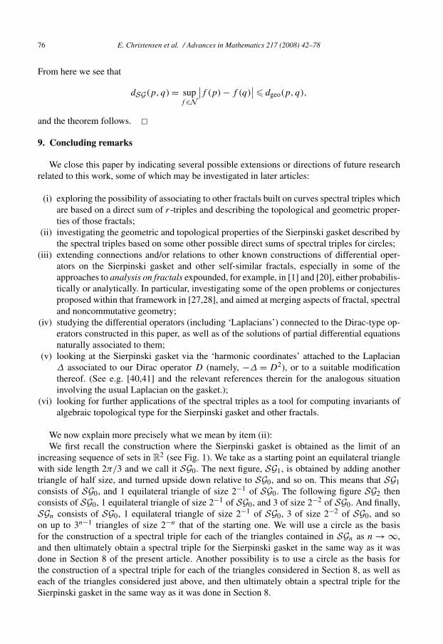
76 E. Christensen et al. / Advances in Mathematics 217 (2008) 42–78
From here we see that
dSG(p, q) = supf ∈N
∣∣f (p) − f (q)∣∣ � dgeo(p, q),
and the theorem follows. �9. Concluding remarks
We close this paper by indicating several possible extensions or directions of future researchrelated to this work, some of which may be investigated in later articles:
(i) exploring the possibility of associating to other fractals built on curves spectral triples whichare based on a direct sum of r-triples and describing the topological and geometric proper-ties of those fractals;
(ii) investigating the geometric and topological properties of the Sierpinski gasket described bythe spectral triples based on some other possible direct sums of spectral triples for circles;
(iii) extending connections and/or relations to other known constructions of differential oper-ators on the Sierpinski gasket and other self-similar fractals, especially in some of theapproaches to analysis on fractals expounded, for example, in [1] and [20], either probabilis-tically or analytically. In particular, investigating some of the open problems or conjecturesproposed within that framework in [27,28], and aimed at merging aspects of fractal, spectraland noncommutative geometry;
(iv) studying the differential operators (including ‘Laplacians’) connected to the Dirac-type op-erators constructed in this paper, as well as of the solutions of partial differential equationsnaturally associated to them;
(v) looking at the Sierpinski gasket via the ‘harmonic coordinates’ attached to the LaplacianΔ associated to our Dirac operator D (namely, −Δ = D2), or to a suitable modificationthereof. (See e.g. [40,41] and the relevant references therein for the analogous situationinvolving the usual Laplacian on the gasket.);
(vi) looking for further applications of the spectral triples as a tool for computing invariants ofalgebraic topological type for the Sierpinski gasket and other fractals.
We now explain more precisely what we mean by item (ii):We first recall the construction where the Sierpinski gasket is obtained as the limit of an
increasing sequence of sets in R2 (see Fig. 1). We take as a starting point an equilateral triangle
with side length 2π/3 and we call it SG0. The next figure, SG1, is obtained by adding anothertriangle of half size, and turned upside down relative to SG0, and so on. This means that SG1consists of SG0, and 1 equilateral triangle of size 2−1 of SG0. The following figure SG2 thenconsists of SG0, 1 equilateral triangle of size 2−1 of SG0, and 3 of size 2−2 of SG0. And finally,SGn consists of SG0, 1 equilateral triangle of size 2−1 of SG0, 3 of size 2−2 of SG0, and soon up to 3n−1 triangles of size 2−n that of the starting one. We will use a circle as the basisfor the construction of a spectral triple for each of the triangles contained in SGn as n → ∞,and then ultimately obtain a spectral triple for the Sierpinski gasket in the same way as it wasdone in Section 8 of the present article. Another possibility is to use a circle as the basis forthe construction of a spectral triple for each of the triangles considered in Section 8, as well aseach of the triangles considered just above, and then ultimately obtain a spectral triple for theSierpinski gasket in the same way as it was done in Section 8.

E. Christensen et al. / Advances in Mathematics 217 (2008) 42–78 77
Next, in the special case of the Sierpinski gasket, we elaborate on item (vi) above regardingthe computation of topological invariants:
The spectral triple ST(SG) has been constructed in such a way that the theory of [6, Sec-tions IV.1 and IV.2], will yield nontrivial topological information. The details of this will appearin a later article, but to indicate what sort of results we have in mind, we will just describethe bounded Fredholm module (K-cycle) which one can obtain from ST(SG) = (C(SG),HSG(together with πSG),DSG). The unitary part, FSG , of the polar decomposition of the Diracoperator DSG gives a bounded odd Fredholm module (πSG,HSG,FSG), see [6, Chapter IV,Section 2] and [38]. The pairing with K1(SG) can then be obtained in the following way. LetFSG = P+ − (I − P+), where P+ is the orthogonal projection of HSG onto the eigenspace cor-responding to the positive eigenvalues of DSG, and let f be a continuous function on SG whichhas the property that πSG(f ) is invertible, i.e. min{|f (x)| | x ∈ SG} > 0. Then the equicontinu-ity of f will imply that there exists a natural number, say n0, such that for any n � n0 and anytriangle Δn,i of size 2−n that of the original one, the function f has winding number 0 alongΔn,i . This implies that the operator P+πSG(f )P+ has a finite index which actually is the op-posite number to the sum of all the winding numbers over all the triangles Δj,h for 0 � j < n0and h ∈ {1, . . . ,3j }. This is a rather obvious extension of well-known results for the circle, butwe think that also the newer invariants related to the cyclic cohomology of the gasket may beexpressed via the spectral triple ST(SG).
Acknowledgments
We are grateful to Alexander Teplyaev for constructive discussions about analysis on fractalsand for bringing the newly developed theory of ‘quantum graphs’ to our attention, after we hadcompleted a preliminary version of this paper.
Erik Christensen expresses his gratitude towards Gilles Pisier for generous support while hewas visiting Texas A&M University.
References
[1] M.T. Barlow, Diffusions on fractals, in: Lectures on Probability Theory and Statistics, Saint-Flour, 1995, in: SpringerLecture Notes, vol. 1690, 1998, pp. 1–121.
[2] E. Christensen, C. Ivan, Spectral triples for AF C*-algebras and metrics on the Cantor set, J. Operator Theory 56(2006) 17–46.
[3] E. Christensen, C. Ivan, Sums of two dimensional spectral triples, Math. Scand. 100 (2007) 35–60.[4] F. Cipriani, D. Guido, S. Scarlatti, A remark on trace properties of K-cycles, J. Operator Theory 35 (1996) 175–189.[5] A. Connes, Compact metric spaces, Fredholm modules, and hyperfiniteness, Ergodic Theory Dynam. Systems 9
(1989) 207–220.[6] A. Connes, Noncommutative Geometry, Academic Press, San Diego, 1994.[7] A. Connes, Unpublished notes on a Dirac operator associated to the Cantor subset of the unit interval (electronic
message to Michel Lapidus, May 2002).[8] A. Connes, M. Marcolli, A walk in the noncommutative garden, arXiv: math.QA/0601054, 2006.[9] A. Connes, D. Sullivan, Quantized calculus on S1 and quasi-Fuchsian groups, unpublished, 1994.
[10] G. Cornelissen, M. Marcolli, K. Reihani, A. Vdovina, Noncommutative geometry on trees and buildings, arXiv:math.QA/0604114, 2006.
[11] E.B. Davies, Analysis on graphs and noncommutative geometry, J. Funct. Anal. 111 (1993) 398–430.[12] G.A. Edgar, Measure, Topology, and Fractal Geometry, Undergrad. Texts Math., Springer-Verlag, New York, 1990.[13] G.A. Edgar, Integral, Probability, and Fractal Measures, Springer-Verlag, New York, 1998.[14] R.E. Edwards, Fourier Series. A Modern Introduction, vol. 1, second ed., Grad. Texts in Math., vol. 64, Springer-
Verlag, New York, 1979.
78 E. Christensen et al. / Advances in Mathematics 217 (2008) 42–78
[15] K.J. Falconer, Fractal Geometry: Mathematical Foundations and Applications, Wiley, Chichester, 1990.[16] D. Guido, T. Isola, Fractals in noncommutative geometry, in: R. Longo (Ed.), Proc. Conf. “Mathematical Physics in
Mathematics and Physics”, Siena, 2000, in: Fields Inst. Commun., vol. 30, Amer. Math. Soc., 2001, pp. 171–186.[17] D. Guido, T. Isola, Dimensions and singular traces for spectral triples, with applications to fractals, J. Funct.
Anal. 203 (2003) 362–400.[18] D. Guido, T. Isola, Dimensions and spectral triples for fractals in R
n, arXiv: math.OA/0404295 v2, 2005.[19] R.V. Kadison, J.R. Ringrose, Fundamentals of the Theory of Operator Algebras, vols. I and II, Academic Press,
New York, 1983.[20] J. Kigami, Analysis on Fractals, Cambridge Univ. Press, Cambridge, 2001.[21] J. Kigami, M.L. Lapidus, Weyl’s problem for the spectral distribution of Laplacians on p.c.f. self-similar sets,
Comm. Math. Phys. 158 (1993) 93–125.[22] J. Kigami, M.L. Lapidus, Self-similarity of volume measures for Laplacians on p.c.f. self-similar fractals, Comm.
Math. Phys. 217 (2001) 165–180.[23] P. Kuchment, Quantum graphs I. Some basic structures, Waves Random Media 14 (2004) 107–128.[24] P. Kuchment, Quantum graphs II. Some spectral properties of quantum and combinatorial graphs, J. Phys. A 38
(2005) 4887–4900.[25] M.L. Lapidus, Fractal drum, inverse spectral problems for elliptic operators and a partial resolution of the Weyl–
Berry conjecture, Trans. Amer. Math. Soc. 325 (1991) 465–529.[26] M.L. Lapidus, Vibrations of fractal drums, the Riemann hypothesis, waves in fractal media, and the Weyl–Berry
conjecture, in: B.D. Sleeman, R.J. Jarvis (Eds.), Ordinary and Partial Differential Equations, in: Pitman Res. NotesMath., vol. 325, 1993, pp. 126–209.
[27] M.L. Lapidus, Analysis on fractals, Laplacians on self-similar sets, noncommutative geometry and spectral dimen-sions, Topol. Methods Nonlinear Anal. 4 (1994) 137–195.
[28] M.L. Lapidus, Towards a noncommutative fractal geometry? Laplacians and volume measures on fractals, in: Har-monic Analysis and Nonlinear Differential Equations, in: Contemp. Math., vol. 208, Amer. Math. Soc., 1997,pp. 211–252.
[29] M.L. Lapidus, M. van Frankenhuijsen, Fractal Geometry and Number Theory: Complex Dimensions of FractalsStrings and Zeros of Zeta Functions, Birkhäuser, Boston, 2000.
[30] M.L. Lapidus, M. van Frankenhuijsen, Fractal Geometry, Complex Dimensions and Zeta Functions: Geometry andSpectra of Fractals Strings, Springer Monogr. Math., Springer-Verlag, New York, 2006.
[31] M.L. Lapidus, H. Maier, The Riemann hypothesis and inverse spectral problems for fractal strings, J. London Math.Soc. (2) 52 (1995) 15–34.
[32] M.L. Lapidus, C. Pomerance, The Riemann zeta-function and the one-dimensional Weyl–Berry conjecture for frac-tal drums, Proc. London Math. Soc. (3) 66 (1993) 41–69.
[33] M. Requardt, Dirac operators and the calculation of the Connes metric on arbitrary (infinite) graphs, J. Phys. A 35(2002) 759–779.
[34] M.A. Rieffel, Comments concerning non-commutative metrics, Talk given at an AMS Special Session, Texas A&M,1993.
[35] M.A. Rieffel, Metrics on states from actions of compact groups, Doc. Math. 3 (1998) 215–229.[36] M.A. Rieffel, Metrics on state spaces, Doc. Math. 4 (1999) 559–600.[37] M.A. Rieffel, Compact quantum metric spaces, in: Operator Algebras, Quantization, and Non-Commutative Geom-
etry, in: Contemp. Math., vol. 365, Amer. Math. Soc., 2004, pp. 315–330.[38] E. Schrohe, M. Walze, J.M. Warzecha, Construction de triplets spectraux à partir de modules de Fredholm, C. R.
Acad. Sci. Paris Sér. I Math. 326 (1998) 1195–1199.[39] R.S. Strichartz, Analysis on fractals, Notices Amer. Math. Soc. (10) 46 (1999) 1199–1208.[40] A. Teplyaev, Energy and Laplacian on the Sierpinski gasket, in: M.L. Lapidus, M. van Frankenhuijsen (Eds.), Fractal
Geometry and Applications: A Jubilee of Benoît Mandelbrot, in: Proc. Sympos. Pure Math., vol. 72, Amer. Math.Soc., 2004, pp. 131–154.
[41] A. Teplyaev, Harmonic coordinates on fractals with finitely ramified cell structure, arXiv: math.PR/0506261, 2006.