direct integration of field equations

Progress In Electromagnetics Research, PIER 28, 339–359, 2000

DIRECT INTEGRATION OF FIELD EQUATIONS

C. T. Tai

Radiation LaboratoryDepartment of Electrical Engineering and Computer ScienceThe University of MichiganAnn Arbor, MI 48109-2122, USA

1. Introduction2. Scalar-Vector Green’s Theorem3. Electrostatics4. Magnetostatics5. Electromagnetics6. Franz’s Original Formulas and Their Derivation

Including the Source Terms7. ConclusionAppendix 1: A Scalar-Vector Green’s TheoremAppendix 2: Franz’s Diffraction Integrals and the Complete

Expressions of the Electromagnetic FieldReferences

1. INTRODUCTION

The direct integration of field equations is first treated in this workwith the aid of a scalar-vector Green’s theorem. In such a treatment,potential functions are not needed, but the result can be interpretedin terms of these functions. The advantage of this approach is toeliminate several concepts that are often difficult for students to di-gest, such as the double layer of charges to characterize an apertureelectrostatic field, the fictitious magnetic surface current to model atangential electric field distribution, and the gauge conditions for thepotential functions in magnetostatics and electrodynamics.

340 Tai

Our method follows closely the original work of Stratton and Chu[1]. We first derive a scalar-vector Green’s theorem with no restrictionplaced on the two functions involved in the theorem. The theorem isthen applied separately to electrostatics, magnetostatics, and finallyto electrodynamics. The result of the last case is identical to the oneoriginally formulated by Stratton and Chu. They are also equivalent tothe expressions obtained by Schelkunoff [2] with the aid of equivalenceprinciple.

When the tangential components of the electromagnetic field arediscontinuous on the diffracting surface, Stratton and Chu deliberatelyadded a line integral to the expression for the electric field and anotherone to the expression for the magnetic field to make them satisfy Max-well’s equations. This amendment was criticized by Schelkunoff, whoclaimed that his formulas were stronger. In fact, as we show in thiswork, Schelkunoff’s expressions are equivalent to Stratton and Chu’s;hence, his formulas are also restricted to continuous surface field dis-tributions. A superior formulation is due to Franz [3], who derived hisformulas with the aid of the free-space magnetic dyadic Green func-tion. We present a detailed comparison between Franz’s formulas andStratton and Chu’s, and show that the line integrals added by Strattonand Chu are contained inherently in Franz’s formulas.

In this article the new differential operational notations for the di-vergence, ∇· , and the curl, ∇× , together with the long-established op-erational notation for the gradient, ∇ , will be used. The rationalefor adopting the new notation for the divergence and the curl is ex-plained thoroughly in [4], particularly from the historical point of viewas discussed in Chapter 8.

2. SCALAR-VECTOR GREEN’S THEOREM

The basic theorem needed in the first part of this work is a scalar-vector Green’s theorem. The theorem involves one scale function andone vector function, hence its name. The derivation of this theoremfrom a vector-dyadic Green’s theorem is found in Appendix 1. Thetheorem states

Direct integration of field equations 341

∫∫

V

∫[(∇· F)∇f + F∇· ∇f + f∇×∇× F]dV

=∫©∫

S

[(n̂ · F)∇f + (n̂ × F) ×∇f + (n̂ ×∇× F)f ]dS (1)

where f is a scalar function and F is a vector function, and all thefunctions are considered to be integrable in V and on S , includingthe generalized functions. We can now apply this theorem to integratethe field equations for various cases.

3. ELECTROSTATICS

We consider a region with a volume charge density ρ and an imaginaryclosed surface Si in which there may be another charge distribution ρi

and/or a scattering body B as shown in Fig. 1. The basic equations in

Figure 1. A charge distribution ρ inside a surface Se in the neigh-borhood of an imaginary surface Si .

electrostatics for the E field in an air medium are

∇· E =ρ

ε0, (2)

∇× E = 0. (3)

Now we apply (1) to integrate (2) under the constraint of (3) withF = E and f = g0 where g0 denotes the free-space scalar Green’s

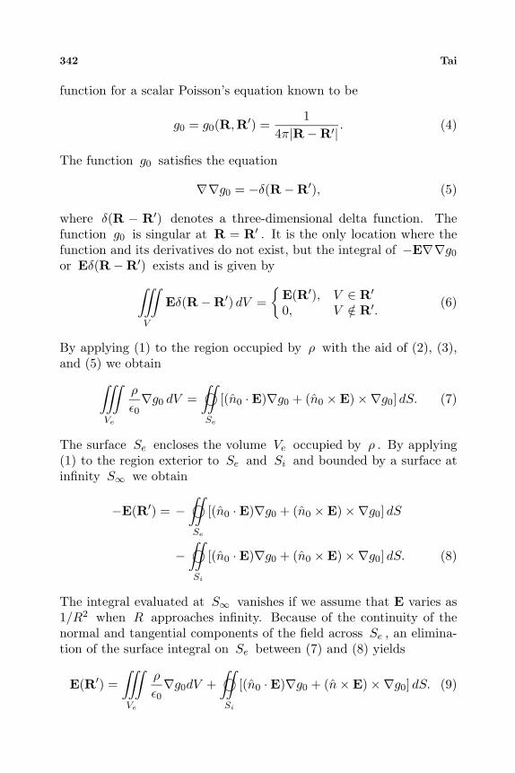
342 Tai

function for a scalar Poisson’s equation known to be

g0 = g0(R,R′) =1

4π|R − R′| . (4)

The function g0 satisfies the equation

∇· ∇g0 = −δ(R − R′), (5)

where δ(R − R′) denotes a three-dimensional delta function. Thefunction g0 is singular at R = R′ . It is the only location where thefunction and its derivatives do not exist, but the integral of −E∇· ∇g0

or Eδ(R − R′) exists and is given by∫∫

V

∫Eδ(R − R′) dV =

{E(R′), V ∈ R′

0, V /∈ R′.(6)

By applying (1) to the region occupied by ρ with the aid of (2), (3),and (5) we obtain

∫∫

Ve

∫ρ

ε0∇g0 dV =

∫©∫

Se

[(n̂0 · E)∇g0 + (n̂0 × E) ×∇g0] dS. (7)

The surface Se encloses the volume Ve occupied by ρ . By applying(1) to the region exterior to Se and Si and bounded by a surface atinfinity S∞ we obtain

−E(R′) = −∫©∫

Se

[(n̂0 · E)∇g0 + (n̂0 × E) ×∇g0] dS

−∫©∫

Si

[(n̂0 · E)∇g0 + (n̂0 × E) ×∇g0] dS. (8)

The integral evaluated at S∞ vanishes if we assume that E varies as1/R2 when R approaches infinity. Because of the continuity of thenormal and tangential components of the field across Se , an elimina-tion of the surface integral on Se between (7) and (8) yields

E(R′) =∫∫

Ve

∫ρ

ε0∇g0dV +

∫©∫

Si

[(n̂0 · E)∇g0 + (n̂ × E) ×∇g0] dS. (9)


Now,∇g0 = −∇′g0, (10)

and∇′g0 × (n̂0 × E) = ∇×′g0(n̂0 × E), (11)

where ∇′ and ∇×′ denote the gradient and the curl operators definedwith respect to the primed variable pertaining to R′ , the site of thefield under consideration, (9) can therefore be written in the form

E(R′) = −∇′∫∫

Ve

∫1ε0

ρg0 dV −∇′∫©∫

Si

(n̂0 · E)g0 dS

+ ∇×′∫©∫

Si

(n̂0 × E)g0 dS. (12)

This is the integral expression of the electric field we are seeking. Ifwe denote

1ε0

∫∫

Ve

∫ρg0 dV +

∫©∫

Si

(n̂0 · E)g0 dS = Φes(R′), (13)

∫©∫

Si

(n̂0 × E)g0 dS = Aes(R′), (14)

thenE(R′) = −∇′Φes(R′) + ∇×′Aes(R′). (15)

Equation (15) shows E(R′) can be evaluated from the differentialsof two potential functions, one representing an electrostatic potential,Φes , and another representing an electrostatic vector potential, Aes .For those who prefer to derive integral expressions by applying theequivalence principle, a topic to be mentioned in a later section, theterm n̂×E in (12) would be interpreted as the equivalent surface mag-netic current density. To introduce a magnetic current in electrostaticswould be very awkward indeed.

The classical treatment of this problem was usually done with theaid of a scalar potential theory. According to this approach, if a scalarpotential function φ is defined at the very beginning such that

E = −∇φ, (16)

344 Tai

then φ satisfies the scalar Poisson’s equation

∇· ∇φ = − ρ

ε0. (17)

The integral expression of (17) for the problem under consideration isfound in many books, for example [1, Sec. 3.4] and [5]. The result is

φ(R′) =1ε0

∫∫

Ve

∫ρg0 dV −

∫©∫

Si

(n̂0 · ∇φ)g0 dS

+∫©∫

Si

(n̂0 · ∇g0)φ dS. (18)

The last term in (18) is commonly interpreted as the potential due toa double layer of charge. Since such a layer does not exist in the actualproblem, this interpretation appears to be very difficult for studentsto appreciate. By taking a gradient of (18) in the primed system andwith the aid of the identity

∇×′∫©∫

Si

(n̂0 × E)g0 dS = −∇′∫©∫

Si

(n̂0 · ∇g0)φ dS, (19)

our (12) can be recovered. The main feature of the present treatmentis a more direct approach of finding E without introducing the poten-tial function. Equation (19) also indicated that the potential functionsare not unique. In our presentation, an electrostatic vector potentialappears quite naturally in the formulation that is absent in the con-ventional theory using φ .

4. MAGNETOSTATICS

We consider a similar problem shown in Fig. 1 with ρ replaced by J,a solenoidal electric current distribution. The basic equations for themagnetostatic H field with J placed in air are given by

∇× H = J, (20)∇· H = 0. (21)


We now apply (1) to this problem with F = H and f = g0 . Byfollowing steps similar to those of the previous case we obtain

H(R′) =∫∫

Ve

∫g0∇× J dV −

∫©∫

Se

(n̂0 × J)g0 dS

+∫©∫

Si

[(n̂0 · H)∇g0 + (n̂0 × H) ×∇g0] dS. (22)

The volume integral in (22) can be changed to

∫∫

Ve

∫g0∇× J dV =

∫∫

Ve

∫[∇× (g0J) −∇g0 × J] dV

=∫©∫

Se

(n̂0 × J)g0 dS −∫∫

Ve

∫∇g0 × J dV

=∫©∫

Se

(n̂0 × J)g0 dS + ∇×′∫∫

Ve

∫goJ dV. (23)

Substituting (23) into (22) and changing ∇g0 to −∇′g0 we obtain

H(R′) = ∇×′∫∫

Ve

∫g0J dV +∇×′

∫©∫

Si

g0(n̂0 ×H) dS −∇′∫©∫

Si

g0(n̂0 ·H) dS.

(24)This is the integral expression for H(R′) that we are seeking. If wedenote

∫∫

Ve

∫g0J dV +

∫©∫

Si

g0(n̂0 × H) dS = Ams, (25)

∫©∫

Si

g0(n̂0 · H) dS = Φms, (26)

thenH(R′) = ∇×′Ams −∇Φms. (27)

From the point of view of potential theory Ams represents a mag-netostatic vector potential function and Φms a magnetostatic scalar

346 Tai

potential function. It is seen that a vector potential function aloneis not sufficient to formulate this problem from the point of view ofpotential theory. The existence of Φms also explains why the scat-tering of a D.C. magnetic field by a magnetic body can be treated bya scalar potential theory [1, Sec. 4.2]. The conventional method offinding H(R′) is to define a vector potential A first and then find theintegral expression for A. Such a presentation is found in [1, Sec. 4.15].

5. ELECTROMAGNETICS

For simplicity, we consider a harmonically oscillating electromagneticfield for this case. The basic equations in Maxwell’s theory are

∇× E = iωµ0H, (28)∇× H = J − iωε0E, (29)

∇· E =ρ

ε0, (30)

∇· H = 0, (31)∇· J = iωρ. (32)

A time factor e−iωt is used in this work. By eliminating E or Hbetween (28) and (29) we obtain

∇×∇× E − k2E = iωµ0J, (33)

and∇×∇× H − k2H = ∇× J. (34)

The wave number k in (33) and (34) is equal to ω(µ0ε0)1/2 . Thestatic sources in Fig. 1 are now replaced by dynamic current sources Jand Ji accompanied by charge densities ρ and ρi .

To find the integral expression for E we let

F = E, (35)

f = G0 =eik|R−R′|

4π|R − R′| , (36)

where G0 denotes the free-space scalar Green’s function that satisfiesthe equation

∇· ∇G0 + k2G0 = −δ(R − R′). (37)


Substituting (35) and (36) into (1) and making use of (28) to (34) weobtain

E(R′) = iωµ0

∫∫

Ve

∫G0J dV − 1

ε0∇′

∫∫

Ve

∫G0ρ dV

+ iωµ0

∫©∫

Si

G0(n̂0 × H) dS −∇′∫©∫

Si

G0(n̂0 · E) dS

+ ∇×′∫©∫

Si

G0(n̂0 × E) dS, (38)

H(R′) =∇×′∫∫

Ve

∫G0J dV + ∇×′

∫©∫

Si

G0(n̂0 × H) dS

−∇′∫©∫

Si

G0(n̂0 · H) dS − iωε0

∫©∫

Si

G0(n̂0 × E) dS. (39)

These are the same equations obtained previously by Stratton and Chuexcept that we have presented them in a slightly different form withthe differential operators ∇′ and ∇×′ placed outside the integrals. Forconvenience, the surface integrals in (38) and (39) will be designatedas the diffraction integrals.

From the point of view of potential theory if we denote

Ae =∫∫

Ve

∫G0J dV +

∫©∫

Si

G0(n̂0 × H) dS, (40)

φe =1ε0

∫∫∫G0ρ dV +

∫©∫

Si

G0(n̂0 · E) dS, (41)

Am =∫©∫

Si

G0(n̂0 × E) dS, (42)

φm =∫©∫

Si

G0(n̂0 · H) dS, (43)

then

E(R′) = iωµ0Ae −∇′φe + ∇×′Am, (44)H(R′) = −iωε0Am −∇′φm + ∇×′Ae. (45)

348 Tai

It can be shown that when the fields are continuous on Si we have thegauge condition

∇· ′Ae = iωε0φe, (46)∇· ′Am = −iωµ0φm, (47)

Then (44) and (45) can be written in the form

E(R′) = iωµ0Ae +i

ωε0∇′∇· ′Ae + ∇×′Am, (48)

H(R′) = −iωε0Am − i

ωµ0∇′∇· ′Am + ∇×′Ae. (49)

The surface integrals in (48) and (49) are the same expressions obtainedby Schelkunoff [2] using the method of potentials with the aid of theequivalence principle [6]. The function F in his expressions, (18) and(19) of [2], corresponds to our −Am , and his A corresponds to thesurface integral in our Ae . Schelkunoff uses eiωt as the time factor incontrast to our e−iωt , which is also used by Stratton and Chu. Whenthe electromagnetic fields, E and H, are discontinuous on Si , (46)and (47) are no longer applicable. Schelkunoff’s formulas also becomeinapplicable, since they are derived under these conditions.

For discontinuous H field on Si let us consider the surface integralin (40). Its divergence is

∇· ′∫©∫

Si

G0(n̂0 × H) dS =∫©∫

Si

n̂0 · (∇G0 × H) dS

=∫©∫

Si

n̂0 · [∇×(G0H) − G0∇× H] dS. (50)

Let C be the line contour separating the closed surface Si into twoopen surfaces S1 and S2 across which H is discontinuous. Then

∫©∫

Si

n̂0 · ∇× (G0H) =∮

CG0(H1 − H2) · d�,

and ∫©∫

Si

n̂0 · (−G0∇× H) dS = iωε0

∫©∫

Si

G0(n̂0 · E) dS,


hence

∇· ′Ae = iω

∫∫

V

∫G0ρ dv + iωε0

∫©∫

Si

G0(n̂0 · E) dS

+∮

CG0(H1 − H2) · d�1

= iωε0φe +∮

CG0(H1 − H2) · d�1. (51)

Similarly, when E is discontinuous on Si

∇· ′Am = −iωµ0φm +∮

CG0(E1 − E2) · d�1. (52)

Substituting the functions φe and φm from (51) and (52) into (44)and (45), we obtain

E(R′) = iωµ0Ae +i

ωε0∇′∇· ′Ae + ∇×′Am

+i

ωε0∇′

∮C

G0(H1 − H2) · d�1, (53)

H(R′) = − iωε0Am − i

ωµ0∇′∇· ′Am + ∇×′Ae

− i

ωµ0∇′

∮C

G0(E1 − E2) · d�1. (54)

Because Ae and Am satisfy the differential equations

∇· ′∇′Ae + k2Ae = 0,

∇· ′∇′Am + k2Am = 0,

when R′ is not located in Si , the first two terms in (53) and (54) canbe changed to

iωµ0Ae +i

ωε0∇′∇· ′Ae = − iωµ0

k2∇· ′∇′Ae +

i

ωε0∇′∇· ′Ae

=i

ωε0(∇′∇· ′Ae −∇· ′∇′Ae)

=i

ωε0∇×′∇×′Ae, (55)

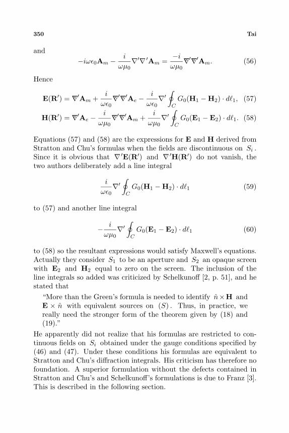
350 Tai

and−iωε0Am − i

ωµ0∇′∇· ′Am =

−i

ωµ0∇×′∇×′Am. (56)

Hence

E(R′) = ∇×′Am +i

ωε0∇×′∇×′Ae −

i

ωε0∇′

∮C

G0(H1 − H2) · d�1, (57)

H(R′) = ∇×′Ae −i

ωµ0∇×′∇×′Am +

i

ωµ0∇′

∮C

G0(E1 − E2) · d�1. (58)

Equations (57) and (58) are the expressions for E and H derived fromStratton and Chu’s formulas when the fields are discontinuous on Si .Since it is obvious that ∇· ′E(R′) and ∇· ′H(R′) do not vanish, thetwo authors deliberately add a line integral

i

ωε0∇′

∮C

G0(H1 − H2) · d�1 (59)

to (57) and another line integral

− i

ωµ0∇′

∮C

G0(E1 − E2) · d�1 (60)

to (58) so the resultant expressions would satisfy Maxwell’s equations.Actually they consider S1 to be an aperture and S2 an opaque screenwith E2 and H2 equal to zero on the screen. The inclusion of theline integrals so added was criticized by Schelkunoff [2, p. 51], and hestated that

“More than the Green’s formula is needed to identify n̂×H andE × n̂ with equivalent sources on (S) . Thus, in practice, wereally need the stronger form of the theorem given by (18) and(19).”

He apparently did not realize that his formulas are restricted to con-tinuous fields on Si obtained under the gauge conditions specified by(46) and (47). Under these conditions his formulas are equivalent toStratton and Chu’s diffraction integrals. His criticism has therefore nofoundation. A superior formulation without the defects contained inStratton and Chu’s and Schelkunoff’s formulations is due to Franz [3].This is described in the following section.


6. FRANZ’S ORIGINAL FORMULAS AND THEIRDERIVATION INCLUDING THE SOURCE TERMS

In Franz’s original work he considers the integration of Maxwell’s equa-tions in a source-free region outside of Si in Fig. 1 with J = 0 , andρ = 0 in (29) and (30). He then applies the method of dyadic Greenfunction to integrate the homogeneous Maxwell’s equations, namely

∇×E = iωµ0H (61)

and∇×H = −iωε0E. (62)

The dyadic Green function that he used is what we designate nowadaysas the free-space magnetic dyadic Green function [7, p. 60] defined by

¯̄Gm0(R,R′) = ∇×[¯̄IG0

]= ∇G0 × ¯̄I, (63)

where G0 is the same scalar Green function defined by (36) and ¯̄I isthe idem factor. He then applies the vector-dyadic Green’s theorem ofthe form ∫∫

V

∫ [F · ∇×∇× ¯̄G − (∇×∇× F) · ¯̄G

]dV

=∫©∫

Si

n̂0 ·[F ×∇× ¯̄G + (∇× F) × ¯̄G

]dS (64)

to integrate (61) and (62) with F = E or H and ¯̄G = ¯̄Gm0 . He didnot provide many details in his article but merely presented his resultas follows:

Ef (R′) = ∇×′Am +i

ωε0∇×′∇×′Ase, (65)

Hf (R′) = ∇×′Ase −i

ωµ0∇×′∇×′Am, (66)

where Am is the same function defined by (42) and Ase is the surfaceintegral in (40), that is,

Ase =∫©∫

Si

G0(n̂0 × H) dS. (67)

352 Tai

No volume integral occurs in his formulation. For completeness wehave filled in the details of Franz’s work in Appendix 2. In order tocompare Franz’s with Stratton and Chu’s formulation we also includethe sources J and ρ . The proper dyadic Green function to integratethe equation for E is the free-space electric dyadic Green functiondefined by

¯̄Ge0(R,R′) =(

¯̄I +1k2

∇∇)

G0. (68)

The expression for E can also be obtained by integrating the equationfor H using ¯̄Gm0 . The integration of Maxwell’s equations using ¯̄Ge0

was briefly introduced by the present author on two previous occasions[8, 9]. The same method was used by Sancer [10], whose results will bequoted later. The detailed analysis of Franz’s formulation and ours aregiven in Appendix 2. We are using the notation Ef to denote Franz’sdiffraction integrals as in (65) and (66) and the complete formulasincluding the contributions by sources J and ρ as EF and HF ,then one finds

EF (R′) = ∇×′Am +i

ωε0∇×′∇×′Ae, (69)

HF (R′) = ∇×′Ae −i

ωµ0∇×′∇×′Am, (70)

where Ae and Am are the functions defined previously by (40) and(41). Comparing (69) and (70) with Stratton and Chu’s formulas wefind

EF = Esc +i

ωε0∇′

∮C

G0(H1 − H2) · d�, (71)

HF = Hsc −i

ωµ0∇′

∮C

G0(E1 − E2) · d�. (72)

For clarity, we have used the subscript “sc” to denote Stratton andChu’s expressions. It is evident that Franz’s formulas thus derived aresuperior because they are applicable to continuous or discontinuousdistribution of the fields on Si and they do satisfy Maxwell’s equations.It should be mentioned that (71) and (72) are identical to the formulasobtained independently by Sancer [10, Eqs. (2.24) and (2.25)] basedalso on the method of ¯̄Ge0 . He did not convert them to a compactform as described by (69) and (70). His article contains much more


useful information not covered here. As a whole we must give credit toFranz for his elegant formulation of the vectorial Huygens’s principle.

The reader may be interested to note that by taking the curl of (71)and (72) we find

∇× Esc = ∇× EF = iωµ0HF (73)

and∇× Hsc = ∇× HF = J − iωε0EF . (74)

In other words, it is possible to find EF and HF from Hsc and Esc ,respectively. This feature was pointed out in a previous communication[9] without the detailed analysis as found in the present article.

7. CONCLUSION

In this work we have studied quite thoroughly the integration of fieldequations in electrostatics, magnetostatics, and electromagnetics, firstbased on a scalar-vector Green’s theorem and then by a vector-dyadicGreen’s theorem for the electromagnetic equations. Some deficien-cies in past works of Stratton and Chu and of Schelkunoff have beenpointed out. The superior nature of Franz’s formulation is emphasized.This investigation demonstrates clearly that the so-called equivalenceprinciple does not serve a useful purpose in the teaching of electromag-netics.

It is worth mentioning that for physically realizable problems theline integrals added by Stratton and Chu are of no concern to usnowadays as a result of Meixner’s edge condition [11]. Collin [12,Sec. 1.5] has examined very carefully a canonical problem using cylin-drical waves to demonstrate the continuity of E and H across theboundary of a conducting wedge. When approximate distribution isused, such as the one that occurred in physical optics approximationwhere S1 corresponds to a lit region and S2 to a completely shad-owed region, then the line integrals must be added to both Strattonand Chu’s and Schelkunoff’s formulas while Franz’s formulas coverthem automatically. A remark made by the master physicist ArnoldSommerfeld in his recapitulation of Franz’s formulation [13, p. 328]may be of interest in this regard:

“The vectorial Huygen’s principle is no magic wand for the solu-tion of boundary value problems, but it is of interest as a gener-alization of the time-honored idea of Christian Huyens.”

354 Tai

The classical work of Levine and Schwinger [14] to treat the diffractionof a plane electromagnetic wave by a circular hole in a conductingscreen as a boundary-value problem attests the master’s view.

APPENDIX 1: A SCALR-VECTOR GREEN’S THEOREM

This theorem can be derived in several different ways. The most effi-cient one is to use a vector-dyadic Green’s theorem of the second kind[4, p. 125] in the form∫∫

V

∫ [F · ∇×∇× ¯̄G − (∇×∇× F) · ¯̄G

]dV

= −∫©∫

S

n̂ ·[F ×∇× ¯̄G + (∇× F) × ¯̄G

]dS. (A.1)

This theorem is also needed in explaining Franz’s theory in Appendix2. It is partly for this reason we adopt this approach so that somerudimentary dyadic analysis can be introduced. In (A.1), F is a vectorfunction and ¯̄G is a dyadic function. Let

¯̄G = f ¯̄I, (A.2)

where f is a scalar function and where ¯̄I denotes an idemfactor de-fined by

¯̄I =∑

i

x̂ix̂i, (A.3)

in a rectangular coordinate system or any orthogonal curvilinear sys-tem. The idemfactor has the property

F · ¯̄I = ¯̄I · F = F. (A.4)

In the following analysis we also need a dyadic identity

a · (b × ¯̄c) = (a × b) · ¯̄c = −b · (a × ¯̄c). (A.5)

In this identity the dyadic function ¯̄c must be kept at the posteriorposition unless it is a symmetric dyadic function. The gradient, diver-gence, and curl of ¯̄G are then given by

∇ ¯̄G = ∇(f ¯̄I

)= (∇f) ¯̄I, (A.6)

∇· ¯̄G = ∇·(f ¯̄I

)= ∇f · ¯̄I = ∇f, (A.7)

∇× ¯̄G = ∇×(f ¯̄I

)= ∇f × ¯̄I, (A.8)


and

n̂ ·(F ×∇× ¯̄G

)= (n̂ × F) · ∇× ¯̄G = (n̂ × F) ·

(∇f × ¯̄I

)= (n̂ × F) ×∇f,

(A.9)

F · ∇×∇× ¯̄G = F ·(∇∇· ¯̄G −∇· ∇ ¯̄G

)

= F · ∇∇f − F∇· ∇f = ∇· (F∇f) −∇· F∇f − F∇· ∇f.

(A.10)

One can easily recognize that these identities are the dyadic version ofsimilar identities in vector analysis. The volume integral of the term∇· (F∇f) in (A.10) can be converted into a surface integral by meansof the dyadic divergence theorem, that is,∫∫

V

∫∇· (F∇f) dV =

∫©∫

n

(n̂ · F)∇f dS. (A.11)

Now substituting all the relevant functions into (A.1) we obtain thedesired scalar-vector Green’s theorem:∫∫

V

∫[(∇· F)∇f + F∇· ∇f + f∇×∇× F] dV

=∫©∫

S

[(n̂ · F)∇f + (n̂ × F) ×∇f + (n̂ ×∇× F)f ] dS. (A.12)

APPENDIX 2: FRANZ’S DIFFRACTION INTEGRALSAND THE COMPLETE EXPRESSIONS OF THEELECTROMAGNETIC FIELD

In Franz’s original work he considers only the homogeneous Maxwell’sequations without the sources in the region of integration bounded bySi and S∞ (Fig. 1). They are

∇× E = iωµ0H, (A.13)∇× H = −iωε0E. (A.14)

By eliminating E or H we obtain

∇×∇× E − k2E = 0, (A.15)∇×∇× H − k2H = 0. (A.16)

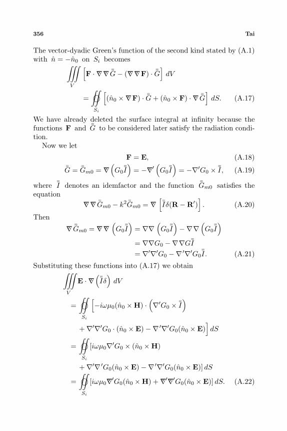
356 Tai

The vector-dyadic Green’s function of the second kind stated by (A.1)with n̂ = −n̂0 on Si becomes∫∫

V

∫ [F · ∇×∇× ¯̄G − (∇×∇× F) · ¯̄G

]dV

=∫©∫

Si

[(n̂0 ×∇× F) · ¯̄G + (n̂0 × F) · ∇× ¯̄G

]dS. (A.17)

We have already deleted the surface integral at infinity because thefunctions F and ¯̄G to be considered later satisfy the radiation condi-tion.

Now we let

F = E, (A.18)¯̄G = ¯̄Gm0 = ∇×

(G0

¯̄I)

= −∇×′(G0

¯̄I)

= −∇′G0 × ¯̄I, (A.19)

where ¯̄I denotes an idemfactor and the function ¯̄Gm0 satisfies theequation

∇×∇× ¯̄Gm0 − k2 ¯̄Gm0 = ∇×[¯̄Iδ(R − R′)

]. (A.20)

Then

∇× ¯̄Gm0 = ∇×∇×(G0

¯̄I)

= ∇∇·(G0

¯̄I)−∇· ∇

(G0

¯̄I)

= ∇∇G0 −∇· ∇G¯̄I= ∇′∇′G0 −∇· ′∇′G0

¯̄I. (A.21)

Substituting these functions into (A.17) we obtain∫∫

V

∫E · ∇×

(¯̄Iδ

)dV

=∫©∫

Si

[−iωµ0(n̂0 × H) ·

(∇′G0 × ¯̄I

)

+ ∇′∇′G0 · (n̂0 × E) −∇· ′∇′G0(n̂0 × E)]dS

=∫©∫

Si

[iωµ0∇′G0 × (n̂0 × H)

+ ∇′∇· ′G0(n̂0 × E) −∇· ′∇′G0(n̂0 × E)] dS

=∫©∫

Si

[iωµ0∇×′G0(n̂0 × H) + ∇×′∇×′G0(n̂0 × E)] dS. (A.22)


The volume integral in (A.22) can be changed to∫∫

V

∫E · ∇×

(¯̄Iδ

)dV =

∫∫

V

∫ [∇· (E × ¯̄Iδ) + ¯̄Iδ · ∇×E

]dS

= ∇×′E = iωµ0H(R′). (A.23)

The integral involving the divergence term in (A.23) vanishes as aresult of the dyadic divergence theorem. We have thus obtained thecelebrated formula of Franz for the H field:

H(R′) = ∇×′∫©∫

Si

G0(n̂0 ×H) dS − i

ωµ0∇×′∇×′

∫©∫

Si

G0(n̂0 ×E) dS. (A.24)

By integrating the equation for H also using ¯̄Gm0 we obtain

E(R′) = ∇×′∫©∫

Si

G0(n̂0 ×E) dS +i

ωε0∇×′∇×′

∫©∫

Si

G0(n̂0 ×H) dS. (A.25)

In the text, these expressions are denoted by Hf and Ef , (65) and(66). We are not certain whether Franz carried out the analysis we dohere because he did not supply the details in his paper. We have usedvery freely the vector and dyadic identities given in [4, Appendix B]omitting the derivations.

In order to compare Stratton and Chu’s or Schelkunoff’s formulawith Franz’s we need the complete expressions for E and H includingthe sources located outside of Si . The equations for E and H arethen given by (33) and (34). We can still use ¯̄Gm0 to integrate theequation for H , which is now given by

∇×∇× H − k2H = ∇× J. (A.26)

The result yields

E(R′) =∫∫∫ (

iωµ0G0J − 1ε0∇′G0ρ

)dV + ∇×′

∫©∫

Si

G0(n̂0 × E) dS

+i

ωε0∇×′∇×′

∫©∫

Si

G0(n̂0 × H) dS. (A.27)

358 Tai

This expression can also be found by integrating the equation for Egiven by

∇×∇× E − k2E = iωµ0J, (A.28)

with the aid of the free-space electric dyadic Green function defined by

¯̄Ge0 =(

¯̄I +1k2

∇∇)

G0. (A.29)

In fact, this is what Sancer [10] did. The expression for H(R′) ob-tained by integrating (A.26) with ¯̄Ge0 yields

H(R′) =∇×′∫∫∫

G0JdV + ∇×′∫©∫

Si

G0(n̂0 × H) dS

− i

ωε0∇×′∇×′

∫©∫

Si

G0(n̂0 × E) dS. (A.30)

In the text, we denote (A.27) and (A.30) by EF and HF respectively.

ACKNOWLEDGMENT

The author is indebted to Dr. Maurice Sancer for a very valuable dis-cussion that helped considerably to improve the presentation of thispaper in its present form. The author would also like to express hissincere gratitude to his late friend Dr. John H. Bryant for his constantencouragement in the early stages of this research.

REFERENCES

1. Stratton, J. A., Electromagnetic Theory, McGraw-Hill, NewYork, 1941. See also Stratton, J. A. and L. J. Chu, “Diffractiontheory of electromagnetic waves,” Phys. Rev., Vol. 56, 99–107,1939.

2. Schelkunoff, S. A., “Kirchoff’s formula, its vector analogue, andother field equivalence theorem,” Proceedings of the Theory ofElectromagnetic Waves Symposium, 43–57, Interscience Publish-ers, New York, 1951.

3. Franz, V. W., “Zur formulierung des huygensschen prinzips,” Z.Naturforsch., A, Vol. 3a, 500–506, 1948.

4. Tai, C. T., Generalized Vector and Dyadic Analysis, Second Edi-tion, IEEE Press and Oxford University Press, New York andoxford, 1997.


5. Webster, A. G., Partial Differential Equations of MathematicalPhysics, 208, Second Edition, Dover Publications, New York,1955.

6. Schelkunoff, S. A., “Some equivalence theorems of electromag-netics and their applications to radiation problems,” B.S.T.J.,Vol. 15, 92–112, 1936.

7. Tai, C. T., Dyadic Green Functions in Electromagnetic Theory,Second Edition, IEEE Press, New York, 1994.

8. Tai, C. T., “A concise formulation of Huygens’s principle for theelectromagnetic field,” IRE Trans. on Antennas and Propagation,Vol. 9, 634, 1960.

9. Tai, C. T., “Kirchoff theory: scalar, vector, or dyadic?” IEEETrans. Antennas Propagat., Vol. AP-20, No. 1, 114–115, 1972.

10. Sancer, M. I., “An analysis of the vector Kirchoff equations andthe associated boundary line charge,” Radio Science, (New Se-ries), Vol. 3, 141–144, 1968.

11. Meixner, J., “Die kantenbedingung in der theorie der beugungelektromagnetischer wellen und volkommen leitenden ebenemschirmen,” Ann. Phys., Vol. 441, 2–9, 1949.

12. Collin, R. E., Field Theory of Guided Waves, IEEE Press andOxford Univ. Press, New York and Oxford, 1991.

13. Sommerfeld, A., Optics, Academic Press, New York, 1954.14. Levine, H. and J. Schwinger, “On the theory of electromag-

netic wave diffraction by an aperture in an infinite plane con-ducting screen,” Theory of Electromagnetic Wave Symposium,1–38,Interscience Publications, New York, 1951.

direct integration of field equations

Documents