direct numerical simulation of turbulent taylor–couette flow

J. Fluid Mech. (2007), vol. 587, pp. 373–393. c© 2007 Cambridge University Press

doi:10.1017/S0022112007007367 Printed in the United Kingdom

373

Direct numerical simulation of turbulentTaylor–Couette flow

S. DONGCenter for Computational and Applied Mathematics, Department of Mathematics,

Purdue University, West Lafayette, IN 47907, USA

(Received 31 January 2007 and in revised form 14 May 2007)

We investigate the dynamical and statistical features of turbulent Taylor–Couette flow(for a radius ratio 0.5) through three-dimensional direct numerical simulations (DNS)at Reynolds numbers ranging from 1000 to 8000. We show that in three-dimensionalspace the Gortler vortices are randomly distributed in banded regions on the wall,concentrating at the outflow boundaries of Taylor vortex cells, which spread overthe entire cylinder surface with increasing Reynolds number. Gortler vortices causestreaky structures that form herringbone-like patterns near the wall. For the Reynoldsnumbers studied here, the average axial spacing of the streaks is approximately 100viscous wall units, and the average tilting angle ranges from 16 to 20. Simulationresults have been compared to the experimental data in the literature, and the flowdynamics and statistics are discussed in detail.

1. IntroductionTaylor–Couette flow becomes particularly complex as the Reynolds number

increases. With increasing Reynolds number, the flow undergoes a series of transitionsfrom circular Couette flow, to axially periodic Taylor vortex flow (Taylor 1923), toa state with waves on the vortices (Coles 1965; Coughlin et al. 1991), to chaoticand turbulent Taylor vortex flow (Coles 1965; Fernstermatcher, Swinney & Gollub1979; Lathrop, Fineberg & Swinney 1992a; von Stamm et al. 1996; Parker & Merati1996; Takeda 1999). In the cases considered in the present paper, the outer cylinderis fixed while the inner cylinder rotates at a constant angular velocity. We focus onvalues of the Reynolds number at which the flow becomes turbulent and small-scaleazimuthal vortices dominate the regions close to both cylinder walls. As there isan overwhelming volume of literature on Taylor–Couette flows (see the review byDiPrima & Swinney 1981 and the references therein), in order to provide a perspectiveon the flow structures and statistics of Taylor–Couette turbulence herein, only relatedexperimental and numerical investigations are reviewed in the sections that follow.

Parameter definitions

It is necessary to first define several parameters before proceeding. The geometry ofthe flow is characterized by the radius ratio, η = R1/R2, where R1 and R2 are the radiiof the inner and outer cylinders respectively, and the aspect ratio, Γ = Lz/d , whereLz is the axial dimension of the domain and d is the gap width, d = R2 − R1. Wedefine the Reynolds number

Re =U0d

ν, (1.1)

374 S. Dong

where U0 is the rotation velocity of the inner cylinder and ν the kinematic viscosityof the fluid. There are several definitions of the Taylor number Ta in the literature.Following Wei et al. (1992), we define it

Ta=(U 2

0 d2/ν2)(d/R1) = Re2

(1

η− 1

). (1.2)

Experimental investigations

Experimental measurement and flow visualization have been the predominant, if notthe exclusive, source of our knowledge about Taylor–Couette flows in the turbulentregime. Insights into the scalings of the torque, velocity structural functions, masstransfer coefficient, and the effects of Reynolds number in Taylor–Couette turbu-lence are provided by the experiments in Wendt (1933), Donnelly & Simon (1959),Bilgen & Boulos (1973), Tam & Swinney (1987), Brandstater & Swinney (1987), Tonget al. (1990), Lathrop, Fineberg & Swinney (1992a, b), Lewis & Swinney (1999), Sheet al. (2001), van den Berg et al. (2003), and Racina & Kind (2006). A detailed analysisof the experimental data from several studies is available in Dubrulle et al. (2005).

Koschmieder (1979) measured the wavelengths of turbulent Taylor vortices (i.e. thedistance between adjacent Taylor vortex pairs) at two radius ratios 0.727 and 0.896,and observed that the wavelength was substantially larger than that of laminar Taylorvortices at the critical onset Taylor number Tc (defined as the Taylor number at whichthe circular Couette flow transitions to the Taylor vortex flow). He also observed theexistence of a continuum of steady non-unique states of the flow, a phenomenonfirst detailed by Coles (1965). The hot-wire anemometry measurements by Smith &Townsend (1982) and Townsend (1984) for a radius ratio 0.667 suggested that forTaylor numbers below 3 × 105Tc turbulent Taylor vortices encircling the inner cylinderdominated the flow and were superimposed on a background of irregular motions.Beyond 5 × 105Tc these turbulent vortices became fragmented and lost regularity, andthe flow became completely turbulent.

Barcilon et al. (1979) studied the coherent structures in Taylor–Couette turbulencewith visualizations for a radius ratio 0.908, and observed a fine herringbone-likepattern of streaks at the outer cylinder wall for Taylor numbers over 400Tc. Theyconjectured that these streaks were the inflow and outflow boundaries of Gortlervortices (Gortler 1954) in the boundary layer region. Assuming a wide separation oflength scales of Taylor and Gortler instabilities at high Taylor numbers, Barcilon &Brindley (1984) proposed a mathematical model by partitioning the flow into interior(Taylor vortex) and boundary layer (Gortler vortex) regions and coupling theseregions through matched asymptotic expansions. They computed the Gortler vortexscales based on this model and demonstrated good comparisons with experimentalobservations. To test the Gortler hypothesis of Barcilon et al. (1979) and Barcilon &Brindley (1984), Wei et al. (1992) performed laser-induced fluorescence flow visuali-zations for three radius ratios (0.084, 0.5 and 0.88) at moderately high Reynoldsnumbers. They observed that Gortler vortices appeared first near the inner cylinderwall, and at Taylor numbers an order of magnitude lower than those in Barcilonet al. (1979). In contrast, Barcilon et al. (1979) observed the herringbone streaksprimarily at the outer cylinder wall, although Barcilon & Brindley (1984) commentedon unpublished studies about observations of herringbone streaks at the inner cylinderwall as well.

Taylor–Couette turbulence 375

Numerical simulations

Compared to experiments, numerical investigations of Taylor–Couette flow in theturbulent regime have lagged far behind. A survey of literature indicates that almostall the numerical simulations so far have concentrated on the laminar regime at lowReynolds numbers, including Taylor vortex flow (Mujumdar & Spalding 1977; Jones1981, 1982; Fasel & Booz 1984; Cliffe & Mullin 1985; Jones 1985; Barenghi & Jones1989; Rigopoulos, Sheridan & Thompson 2003), wavy vortex flow (Marcus 1984a, b;King et al. 1984; Moulic & Yao 1996; Riechelmann & Nanbu 1997; Czarny et al.2004) and modulated wavy vortex flow (Coughlin et al. 1991; Coughlin & Marcus1992a, b). Here we primarily restrict considerations to configurations with a fixedouter cylinder and no imposed axial flow.

Several studies have been conducted at higher Reynolds numbers on ‘turbulentbursts’ (Coughlin & Marcus 1996) and the chaotic behaviour of Taylor–Couette flow(Vastano & Moser 1991). In addition, steady-state quasi-two-dimensional (ignoringazimuthal dependence) Reynolds-averaged Navier–Stokes (RANS) simulations wereperformed by several researchers (Wild, Djilali & Vickers 1996; Batten, Bressloff &Turnock 2002) employing turbulence models.

In order to understand the mechanism of transition from quasi-periodicity to chaosobserved in experiments (Brandstater & Swinney 1987), Vastano & Moser (1991)performed a short-time Lyapunov exponent analysis of the Taylor–Couette flow bysimultaneously advancing the full numerical solution and a set of perturbations for aradius ratio 0.875 at Reynolds numbers between 1160 and 1340. A partial Lyapunovexponent spectrum was computed and the dimension of the chaotic attractor wasestimated. Noting the concentration of perturbation fields on the outflow jet andother characteristics, they argued that the chaos-producing mechanism was a Kelvin–Helmholtz instability of the outflow boundary jet between counter-rotating Taylorvortices. More recently, Bilson & Bremhorst (2007) simulated the Taylor–Couetteflow at Reynolds number 3200 for a radius ratio 0.617 using a second-order finitevolume method. A comprehensive verification for several parameters was conducted,and the comparison with available experimental data showed an agreement of trends.A number of statistical quantities were studied, and results of Reynolds stress budgetsindicated higher turbulence production and dissipation values near cylinder walls.

Objective

In this paper, we focus on the dynamics and statistics of small-scale near-wallazimuthal vortices in turbulent Taylor–Couette flow. For this purpose, we haveperformed three-dimensional direct numerical simulations at four Reynolds numbers,ranging from 1000 to 8000, for a radius ratio η = 0.5. While the flow remains laminarat the lowest Reynolds number Re = 1000, it becomes turbulent for the three higherReynolds numbers. We demonstrate the herringbone-like patterns of streaks nearcylinder walls that are reminiscent of the observations by Barcilon et al. (1979), andelucidate how the increase in Reynolds number affects the characteristics of thesestreaks and the Gortler vortices, as well as the distributions of statistical quantities.

2. Simulation methodology and parametersConsider the incompressible flow between two infinitely long concentric cylinders.

The cylinder axis is aligned with the z-axis of the coordinate system. The innercylinder, with radius R1, rotates counter-clockwise (viewed toward the −z direction)at a constant angular velocity Ω while the outer cylinder, with radius R2, is at rest. In

376 S. Dong

Cases Nz P Lz/d CTinner CTouter

A 128 6 π −0.0125 0.0127B 256 6 2π −0.0126 0.0127C 128 7 π −0.0126 0.0126D 256 7 1.5π −0.0126 0.0126E 256 7 2π −0.0126 0.0127F 128 8 π −0.0128 0.0128G 128 9 π −0.0128 0.0128

Table 1. Grid resolution studies at Re= 8000. Nz, number of Fourier planes in the axialdirection; P , element order; CTinner, mean torque coefficient on inner cylinder wall; CTouter,mean torque coefficient on outer cylinder wall.

the simulations, the coordinates and length variables are normalized by the cylindergap width d; The velocity components are normalized by the rotation velocity of theinner cylinder U0 = ΩR1, and the pressure by ρU 2

0 , where ρ is the fluid density. Sothe Reynolds number is defined by Equation (1.1).

We solve the three-dimensional incompressible Navier-Stokes equations byemploying a Fourier spectral expansion of flow variables in the z-direction (along thecylinder axis), assuming the flow is periodic at z = 0 and z =Lz (the axial dimension ofthe computational domain), and a spectral element discretization (Karniadakis &Sherwin 2005) of the annular domain in (x, y)-planes. For time integration weemploy a stiffly stable velocity-correction-type scheme with a third-order accuracyin time (Karniadakis, Israeli & Orszag 1991). The above numerical scheme hasbeen extensively used to study bluff-body flow and turbulence problems (Dong &Karniadakis 2005; Dong et al. 2006). No-slip boundary conditions are employed onthe inner and outer cylinder walls.

We consider the Taylor–Couette flow at four Reynolds numbers, Re =1000, 3000,5000 and 8000, for a radius ratio η = 0.5. The axial dimension of the computationaldomain is varied between Lz/d = π and 2π. Extensive grid refinement tests have beenconducted. We employ a spectral element mesh with 400 quadrilateral elements inthe (x, y)-planes, and the element order is varied from 6 to 9, with over-integration(Kirby & Karniadakis 2003). In the axial direction we employ 64 to 128 Fouriermodes (or 128 to 256 grid points), with 3/2-dealiasing. These parameters lead to gridspacings near the cylinder surface, in viscous wall units, of 0.21 in the radial direction,1.96 in the azimuthal direction and 3.70 in the axial direction for Re =8000, and0.04 in the radial direction, 0.40 in the azimuthal direction and 0.76 in the axialdirection for Re = 1000. Table 1 summarizes the grid resolution studies at Re= 8000.It shows the mean torque coefficients, averaged over a long time (typically about100 inner-cylinder revolutions), on the inner and outer cylinder walls for differentresolutions. The mean torque coefficient is defined as

CT =〈T 〉

0.5πρU 20 R2

1Lz

(2.1)

where 〈T 〉 is the time-averaged torque on the cylinder walls. From case A to case G,the total degrees of freedom in the simulation have been increased 5-fold. Thetorque is observed to increase slightly and converge to its final value. A comparisonamong cases C to E (and between cases A and B) indicates that the mean torquecoefficient is not very sensitive to the axial dimension of the domain (variation less


tU0/d

CT

5200 5300 5400 5500 5600 5700 5800 5900

0.014

0.016

0.018

0.020

0.022

0.024

Inner cylinder

Outer cylinder

(a) (b)

Re2000 4000 6000 8000

0.02

0.04

0.06

DNS

Wendt’s (1933) empirical relation

Bilgen & Boulos’ (1973) empirical relation

Racina & Kind’s (2006) empirical relation

CT

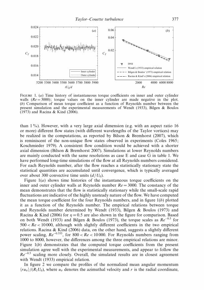
Figure 1. (a) Time history of instantaneous torque coefficients on inner and outer cylinderwalls (Re= 3000); torque values on the inner cylinder are made negative in the plot.(b) Comparison of mean torque coefficient as a function of Reynolds number between thepresent simulation and the experimental measurements of Wendt (1933), Bilgen & Boulos(1973) and Racina & Kind (2006).

than 1 %). However, with a very large axial dimension (e.g. with an aspect ratio 16or more) different flow states (with different wavelengths of the Taylor vortices) maybe realized in the computations, as reported by Bilson & Bremhorst (2007), whichis reminiscent of the non-unique flow states observed in experiments (Coles 1965;Koschmieder 1979). A consistent flow condition would be achieved with a shorteraxial dimension (Bilson & Bremhorst 2007). Simulations at lower Reynolds numbersare mainly conducted with the same resolutions as case E and case G in table 1. Wehave performed long-time simulations of the flow at all Reynolds numbers considered.For each Reynolds number, after the flow reaches a statistically stationary state thestatistical quantities are accumulated until convergence, which is typically averagedover about 300 convective time units (d/U0).

Figure 1(a) shows time histories of the instantaneous torque coefficients on theinner and outer cylinder walls at Reynolds number Re =3000. The constancy of themean demonstrates that the flow is statistically stationary while the small-scale rapidfluctuations are indicative of the highly unsteady nature of the flow. We have computedthe mean torque coefficient for the four Reynolds numbers, and in figure 1(b) plottedit as a function of the Reynolds number. The empirical relations between torqueand Reynolds number determined by Wendt (1933), Bilgen & Boulos (1973) andRacina & Kind (2006) for η = 0.5 are also shown in the figure for comparison. Basedon both Wendt (1933) and Bilgen & Boulos (1973), the torque scales as Re−0.5 for500 < Re< 10 000, although with slightly different coefficients in the two empiricalrelations. Racina & Kind (2006) data, on the other hand, suggests a slightly differentpower scaling, Re−0.555, for 800 < Re< 10 000. For Reynolds numbers ranging from1000 to 8000, however, the differences among the three empirical relations are minor.Figure 1(b) demonstrates that the computed torque coefficients from the presentsimulation agree well with the experimental measurements, and appear to follow theRe−0.5 scaling more closely. Overall, the simulated results are in closest agreementwith Wendt (1933) empirical relation.

In figure 2 we compare the profiles of the normalized mean angular momentum〈ruθ〉/(R1U0), where uθ denotes the azimuthal velocity and r is the radial coordinate,

378 S. Dong

(r-R1)/(R2-R1)

ru

θ

/(R

1U0)

0.2 0.4 0.6 0.8 1.00

0.2

0.4

0.6

0.8

1.0

DNS, Re = 8000

Smith & Townsend (1982), Re = 8698

Smith & Townsend (1982), Re = 17295

Figure 2. Comparison of normalized mean angular momentum profiles between presentsimulation (Re= 8000) and the experiment of Smith & Townsend (1982). uθ is the azimuthalvelocity.

between the present simulation at Re = 8000 and the experiment of Smith &Townsend (1982). Smith & Townsend (1982) measured the mean angular momentumat several Reynolds numbers. The experimental data for the lowest Reynoldsnumber, Re= 8698, in Smith & Townsend (1982) have been included in figure 2 forcomparison. Because Smith & Townsend’s (1982) data at this Reynolds number areavailable only for the region near the inner cylinder, in figure 2 we have also includeddata for the second lowest Reynolds number Re = 17 295 in the experiment for themiddle region of the gap. The computed profile from the current simulation agreeswith Smith & Townsend’s (1982) data reasonably well. The result shows that the coreof the flow (0.1 (r − R1)/(R2 − R1) 0.9) has an essentially constant mean angularmomentum 0.5R1U0, a phenomenon in turbulent Taylor–Couette flow also observedby Lewis & Swinney (1999) at higher Reynolds numbers. The computed angularmomentum profile has a slightly positive slope in the core of the flow, consistentwith the experimental measurement. However, this slope is slightly smaller than thatfrom the experiment (figure 2). It should be noted that Smith & Townsend’s (1982)data are at a radius ratio η =0.667 which is a little different from that in the currentsimulations (η = 0.5). This difference is probably the cause of the slight difference inthe slope of the profile between the simulation and the experiment.

3. Gortler vortices and herringbone streaksIn this section we investigate the flow structures in turbulent Taylor–Couette flow

in detail. Emphasis is placed on the discussion of small-scale vortices near cylinderwalls and the related effects. At each Reynolds number we monitor the signal of thetorque on both cylinder walls (see figure 1a) during the simulation, and ensure thatthe flow has reached a statistically stationary state. All the results presented beloware collected for statistically stationary states.

Figure 3 shows snapshots of instantaneous velocity fields in a radial–axial plane(r, z plane, where r is the radial coordinate), from left to right at Reynolds numbers


r

z

1.0 1.5 2.00

1

2

3

r1.0 1.5 2.0

0

1

2

3

r1.0 1.5 2.0

0

1

2

3

r1.0 1.5 2.0

0

1

2

3

Figure 3. Instantaneous velocity fields in a radial–axial plane at Reynolds numbers(from left to right) Re= 1000, 3000, 5000 and 8000.

Re = 1000, 3000, 5000 and 8000 (a time-averaged flow field will be shown later in§ 4). Inner and outer cylinder walls correspond to r/d = 1.0 and 2.0, respectively. Thevelocity vectors have been plotted on the quadrature points of the spectral elements.The ‘stripes’ in the patterns are due to the non-uniform distribution of spectralelements in the radial direction (finer elements near both walls, coarser elementstoward the middle of the gap) and the non-uniform distribution of quadrature pointswithin an element (finer near element boundaries, coarser in the middle of an element).At Re =1000, large-scale Taylor vortices are observed to occupy the entire gap, withwell-defined inflow and outflow boundaries between the vortex cells. As the Reynoldsnumber increases to 3000, the Taylor vortices become severely distorted. Althoughnot as well-defined as at Re = 1000, a Taylor vortex cell can still be clearly identified,with some cells consisting of two or more smaller vortices rotating in contiguousdirections. In addition, azimuthal vortices with scales significantly smaller than theTaylor vortex, Gortler vortices, emerge on the inner cylinder wall around distortedoutflow boundaries of the Taylor vortex cells. These vortices are absent from theouter cylinder wall at this Reynolds number.

At Re= 5000, the core of the flow is characterized by the presence of a numberof vortices, apparently randomly distributed and with scales significantly smallerthan the gap width. It is not obvious how to identify a large-scale Taylor vortex inthis case. Based on the sense of rotation of vortices, large-scale ‘Taylor cells’, eachencompassing a pack of vortices, may be vaguely recognized, but the ‘boundaries’between cells are highly distorted and in some cases interrupted by vortices near thewall. The number of small-scale vortices near the inner cylinder increases, and theygenerate energetic fluid motions normal to the wall. Although these near-wall vorticesappear to concentrate on the highly distorted outflow boundaries between ‘Taylorcells’, they are also observed in other regions of the wall such as near the inflow

380 S. Dong

6

(a)

5

4

3

2

1

0

–2–1012–2–1

012

z

yx 6

(b)

5

4

3

2

1

0

–2–1012–2–1

012

z

yx

z

yx

yx

Figure 4. Iso-surfaces of instantaneous λ2, the intermediate eigenvalue in the vortex identifica-tion method by Jeong & Hussain (1995): (a) Re =5000 and (b) Re= 8000. Two levels are showncorresponding to λ2 = −2 and −3.5.

boundaries. Such small-scale vortices can be observed near the outer cylinder wall aswell at this Reynolds number.

As the Reynolds number increases to Re= 8000, the flow core teems with vortices,and large-scale ‘Taylor cells’ can hardly be distinguished from the instantaneousvelocity field. A large number of small-scale vortices can be observed near the innercylinder, appearing randomly distributed on the wall. The number of small-scalevortices near the outer cylinder has also increased, although it is notably smaller thanat the inner cylinder wall.

The above observation concerning the onset of small-scale Gortler vortices isconsistent with the previous studies. Although Barcilon et al. (1979) first hypothesizedthe existence of Gortler vortices after observing near-wall herringbone-like streaks,it was Wei et al. (1992) who demonstrated that Gortler vortices appeared first atthe inner cylinder wall with increasing Reynolds number. The present results haveconfirmed Wei et al. (1992) observation. The simulation has further suggested thatthese vortices appear first around the outflow boundaries (figure 3). These observationssupport the instability analyses of Coughlin & Marcus (1992b) and Vastano & Moser(1991), who suggested that the outflow boundary jets between the Taylor vorticeswere the most unstable regions in the flow.

To explore the structural characteristics of the near-wall Gortler vortices in three-dimensional space, we plot in figure 4 the iso-surfaces of λ2, the intermediateeigenvalue of the tensor S : S + Ω: Ω (where S and Ω are the symmetric andantisymmetric parts of the velocity gradient respectively) in Jeong & Hussain (1995),and in Figure 5 the iso-surfaces of the instantaneous pressure (near the inner cylinderwall), for Re= 5000 and 8000. A forest of small-scale vortical structures can beclearly observed in the flow, extending along the azimuthal direction. At Re= 5000,


6

(a) (b)

5

4

3

2

1

0

21

0–1

–1

0

1

x

y

z

z

y

x

6

5

4

3

2

1

0

1.5 1.0 0.5–0.50

–1.0 –1.5

–1

0

1

x

y

z

y

x

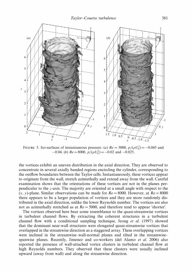
Figure 5. Iso-surfaces of instantaneous pressure: (a) Re = 5000, p/(ρU 20 ) = −0.045 and

−0.04. (b) Re= 8000, p/(ρU 20 ) = −0.02 and −0.025.

the vortices exhibit an uneven distribution in the axial direction. They are observed toconcentrate in several axially banded regions encircling the cylinder, corresponding tothe outflow boundaries between the Taylor cells. Instantaneously, these vortices appearto originate from the wall, stretch azimuthally and extend away from the wall. Carefulexamination shows that the orientations of these vortices are not in the planes per-pendicular to the z-axis. The majority are oriented at a small angle with respect to the(x, y)-plane. Similar observations can be made for Re =8000. However, at Re= 8000there appears to be a larger population of vortices and they are more randomly dis-tributed in the axial direction, unlike the lower Reynolds number. The vortices are alsonot as azimuthally stretched as at Re= 5000, and therefore tend to appear ‘shorter’.

The vortices observed here bear some resemblance to the quasi-streamwise vorticesin turbulent channel flows. By extracting the coherent structures in a turbulentchannel flow with a conditional sampling technique, Jeong et al. (1997) showedthat the dominant near-wall structures were elongated quasi-streamwise vortices thatoverlapped in the streamwise direction as a staggered array. These overlapping vorticeswere inclined in the streamwise–wall-normal planes and tilted in the streamwise–spanwise planes. Recently, Jimenez and co-workers (del Alamo et al. 2006) alsoreported the presence of wall-attached vortex clusters in turbulent channel flow athigh Reynolds numbers. They observed that these clusters were usually inclinedupward (away from wall) and along the streamwise direction.

382 S. Dong

z–d

50 55 60 65 70 750

2

4

6(a)

0

1

2

3

4

5

6(b)

0

2

4

6(c)

(t-t0)U0/d

0

2

4

6(d)

z–d

50 55 60 65 70 75

z–d

50 55 60 65 70 75

z–d

50 55 60 65 70 75

Figure 6. Herringbone-like streaks demonstrated by spatial–temporal plots of the azimuthalvelocity along a fixed line oriented in the z-direction a distance 0.033d away from the innercylinder wall. Shown are azimuthal velocity contours at 8 equi-levels between 0.65U0 and 0.9U0

for (a) Re =1000, (b) Re= 3000, (c) Re= 5000, (d) Re= 8000.

Figure 6 demonstrates the spatial–temporal characteristics of the azimuthal velocity.The velocity data were collected along a fixed line oriented in the z-directionand located near the inner cylinder wall (at a distance 0.033d). Shown are theinstantaneous azimuthal velocity contours in the spatial-temporal (t, z)-plane forReynolds numbers from Re = 1000 to 8000, with uθ/U0|min = 0.65, uθ/U0|max = 0.9and an increment uθ/U0 = 0.0357 between contour levels. At Re =1000, the contourlines are clustered around axial locations that coincide with the outflow boundariesbetween Taylor vortex cells, indicative of persistent high azimuthal velocity valuesin those regions. Localized ‘defects’ can be observed in the distribution, indicatingoccasional disturbances to the flow that die down over time. For Reynolds numbersRe= 3000 and above, intriguing herringbone-like patterns of streaks can be observed


Ω2R42/y2

Til

ting

ang

le o

f st

reak

s (d

eg.)

109 10100

5

10

15

20

25

Present DNS, radius ratio = 0.5

Barcilon & Brindley (1984), radius ratio = 0.712



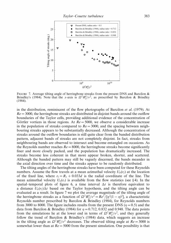
Figure 7. Average tilting angle of herringbone streaks from the present DNS and Barcilon &Brindley’s (1984). Note that the x-axis is Ω2R4

2/ν2, as prescribed by Barcilon & Brindley

(1984).

in the distribution, reminiscent of the flow photographs of Barcilon et al. (1979). AtRe = 3000, the herringbone streaks are distributed in disjoint bands around the outflowboundaries of the Taylor cells, providing additional evidence of the concentration ofGortler vortices in those regions. At Re = 5000, we observe a considerable increasein the population of streaks compared to Re = 3000, and the spacing between neigh-bouring streaks appears to be substantially decreased. Although the concentration ofstreaks around the outflow boundaries is still quite clear from the banded distributionpattern, adjacent bands of streaks are not completely disjoint. In fact, streaks fromneighbouring bands are observed to intersect and become entangled on occasions. Asthe Reynolds number reaches Re = 8000, the herringbone streaks become significantlyfiner and more closely packed, and the population has dramatically increased. Thestreaks become less coherent in that more appear broken, shorter, and scattered.Although the banded pattern may still be vaguely discerned, the bands meander inthe axial direction over time and the streaks appear to be randomly distributed.

The tilting angles of the herringbone streaks have been computed for these Reynoldsnumbers. Assume the flow travels at a mean azimuthal velocity Uθ (rl) at the locationof the fixed line, where rl =R1 + 0.033d is the radial coordinate of the line. Themean azimuthal velocity Uθ (rl) is available from the flow statistics (see § 4). In thespatial–temporal plots of figure 6, a time interval t is therefore equivalent toa distance Uθ (rl)t based on the Taylor hypothesis, and the tilting angle can beevaluated as a result. In figure 7 we plot the average magnitude of the tilting angle ofthe herringbone streaks as a function of Ω2R4

2/ν2 = Re2/[η2(1 − η)2], a characteristic

Reynolds number prescribed by Barcilon & Brindley (1984), for Reynolds numbersfrom 3000 to 8000. The figure includes results from the present DNS (η = 0.5) and thedata from Barcilon & Brindley (1984) for η = 0.712, 0.832 and 0.948. The data pointsfrom the simulations lie at the lower end in terms of Ω2R4

2/ν2, and they generally

follow the trend of Barcilon & Brindley’s (1984) data, which suggests an increasein the tilting angle as Ω2R4

2/ν2 decreases. The observed tilting angle at Re= 3000 is

somewhat lower than at Re= 5000 from the present simulation. One possibility is that

384 S. Dong

fd/U0

Pow

er s

pect

ral d

ensi

ty

10–2 10–1 100 10110–11

10–10

10–9

10–8

10–7

10–6

10–5

10–4

10–3

Re = 1000

Re = 3000

Re = 5000

Re = 8000

–5/3

(a) (b)

Near outer wall

Mid-point

Near inner wall

–5/3

fd/U0

10–2 10–1 100 101

10–10

10–9

10–8

10–7

10–6

10–5

10–4

10–3

Figure 8. Velocity power spectra. (a) Temporal power spectra of the azimuthal velocity at adistance 0.108d from the inner cylinder wall for different Reynolds numbers. (b) Power spectraof the axial velocity in the middle of the gap, and at two other locations at distance 0.033dfrom the inner and outer cylinder walls, respectively, for Re= 8000.

with decreasing Reynolds number the tilting angle may reach a peak value at somepoint and then decrease as the Reynolds number further decreases, since at sufficientlylow Reynolds numbers the herringbone streaks will disappear, as demonstrated byfigure 6(a) for Re = 1000 in the present simulation and by the flow photographs atlow Taylor numbers in Barcilon et al. (1979).

We next investigate the spectral characteristics of turbulent fluctuations in Taylor–Couette flow. Figure 8(a) shows a comparison of the temporal power spectra of theazimuthal velocity at a distance 0.108d from the inner cylinder wall for Reynoldsnumbers Re= 1000, 3000, 5000 and 8000. Velocity power spectra are computed basedon the time histories of the velocity at ‘history points’, and are averaged over the pointsalong the axial direction with the same radial and azimuthal coordinates. Compared tohigher Reynolds numbers, the spectrum at Re= 1000 lacks significant high-frequencycomponents, with negligible spectral density beyond the peak frequency, indicatingthat the flow remains laminar at this Reynolds number. In contrast, the powerspectra at Re = 3000, 5000 and 8000 all exhibit a broadband distribution which ischaracteristic of a turbulent power spectrum, demonstrating that the flow has becometurbulent at these Reynolds numbers. The power spectrum curves of these threeReynolds numbers essentially collapse onto one at low frequencies (f d/U0 2). Athigh frequencies, the larger the Reynolds number, the higher the power spectraldensity, suggesting more energetic turbulent fluctuations with increasing Reynoldsnumbers.

In figure 8(b) we compare the power spectra of the axial velocity at Re =8000 atthree locations: near the inner cylinder wall (at a distance 0.033d), in the middle of thegap, and near the outer cylinder wall (at a distance 0.033d). Velocity spectra have beenaveraged over points along the axial direction with the same radial and azimuthalcoordinates. Increasingly stronger high-frequency components are observed in thepower spectra with decreasing radial coordinates, indicating an uneven distributionof the intensity of turbulent fluctuations. More energetic turbulent fluctuationsare observed toward the inner cylinder wall. The velocity spectra at Re= 3000and 5000 possess similar characteristics. This demonstrates that turbulence at theinner cylinder wall is substantially stronger than at the outer cylinder in turbulent


–2–1

01

2 –2–1

01

2

z

0

1

2

3

4

5

6

y

x

z

0.950.850.750.650.550.450.350.250.150.05

xy

Figure 9. Contours of instantaneous azimuthal velocity on two near-wall grid surfaces (nearlycylindrical) showing the high-speed streaks on the inner cylinder and low-speed streaks on theouter cylinder (Re= 8000).

Taylor–Couette flow. Note that in the configuration studied in this paper, the innercylinder rotates while the outer cylinder is stationary. Although in plane Couette flowonly the difference between velocities at the two walls is significant, this is not the casein Taylor–Couette flow. The curvature effect causes the asymmetry in the intensitydistribution of turbulent fluctuations.

Streaky structures in near-wall regions are common characteristics of wall-boundedturbulence. In turbulent Taylor–Couette flow the inner cylinder wall teems withhigh-speed streaks while the outer cylinder wall teems with low-speed streaks. Infigure 9 we plot contours of the instantaneous azimuthal velocity on two grid surfaces(nearly cylindrical) near the inner and outer cylinder walls at Re = 8000. Numerousazimuthally elongated streaks with higher azimuthal velocities (high-speed streaks)can be observed on the inner cylinder wall, while on the outer cylinder wall theazimuthal velocity in these streaky regions is lower (low-speed streaks) and thestreaks are considerably fewer. Visually, these streaks are not dissimilar to the near-wall ‘low-speed streaks’ observed in other turbulent flows in simpler geometries suchas a channel. Close examination of the high-speed streaks on the inner cylinderand the low-speed streaks on the outer cylinder, however, reveals their intricateherringbone-like pattern, which is absent from those in turbulent channel flows.

In order to determine the axial spacings of the high-speed and low-speed streakson the cylinder walls, we examine the spatial power spectrum of the velocity. Thespatial spectrum is obtained by computing the spatial FFT of the velocity data alonga line oriented in the axial direction. Figure 10(a) shows the time-averaged spatialpower spectrum of the radial velocity at a line adjacent to the inner cylinder wall (at adistance 0.033d) at Re = 8000. The wavenumber at the sharp peak, kTaylor, is indicativeof the spacing of Taylor cells. In this case it corresponds to three pairs of Taylor

386 S. Dong

kd/(2π)

Spa

tial

pow

er s

pect

ral d

ensi

ty

10–2 10–1 100 101 102

10–7

10–6

kTaylor

kstreaks

Away from wall

Near the wall

(a) (b)

Re

Str

eak

spac

ing

in v

isco

us u

nits

4000 6000 80000

50

100

150

200Inner cylinder wall

Outer cylinde rwall

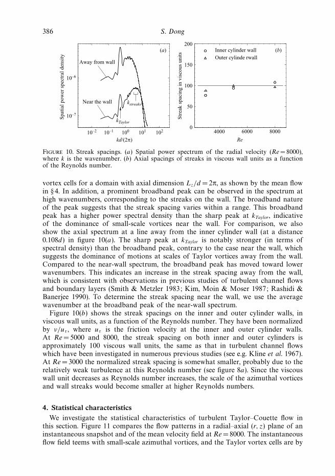
Figure 10. Streak spacings. (a) Spatial power spectrum of the radial velocity (Re= 8000),where k is the wavenumber. (b) Axial spacings of streaks in viscous wall units as a functionof the Reynolds number.

vortex cells for a domain with axial dimension Lz/d = 2π, as shown by the mean flowin § 4. In addition, a prominent broadband peak can be observed in the spectrum athigh wavenumbers, corresponding to the streaks on the wall. The broadband natureof the peak suggests that the streak spacing varies within a range. This broadbandpeak has a higher power spectral density than the sharp peak at kTaylor, indicativeof the dominance of small-scale vortices near the wall. For comparison, we alsoshow the axial spectrum at a line away from the inner cylinder wall (at a distance0.108d) in figure 10(a). The sharp peak at kTaylor is notably stronger (in terms ofspectral density) than the broadband peak, contrary to the case near the wall, whichsuggests the dominance of motions at scales of Taylor vortices away from the wall.Compared to the near-wall spectrum, the broadband peak has moved toward lowerwavenumbers. This indicates an increase in the streak spacing away from the wall,which is consistent with observations in previous studies of turbulent channel flowsand boundary layers (Smith & Metzler 1983; Kim, Moin & Moser 1987; Rashidi &Banerjee 1990). To determine the streak spacing near the wall, we use the averagewavenumber at the broadband peak of the near-wall spectrum.

Figure 10(b) shows the streak spacings on the inner and outer cylinder walls, inviscous wall units, as a function of the Reynolds number. They have been normalizedby ν/uτ , where uτ is the friction velocity at the inner and outer cylinder walls.At Re= 5000 and 8000, the streak spacing on both inner and outer cylinders isapproximately 100 viscous wall units, the same as that in turbulent channel flowswhich have been investigated in numerous previous studies (see e.g. Kline et al. 1967).At Re= 3000 the normalized streak spacing is somewhat smaller, probably due to therelatively weak turbulence at this Reynolds number (see figure 8a). Since the viscouswall unit decreases as Reynolds number increases, the scale of the azimuthal vorticesand wall streaks would become smaller at higher Reynolds numbers.

4. Statistical characteristicsWe investigate the statistical characteristics of turbulent Taylor–Couette flow in

this section. Figure 11 compares the flow patterns in a radial–axial (r, z) plane of aninstantaneous snapshot and of the mean velocity field at Re =8000. The instantaneousflow field teems with small-scale azimuthal vortices, and the Taylor vortex cells are by


r

z

1.0 1.5 2.00

1

2

3

4

5

(a) (b)

r1.0 1.5 2.0

0

1

2

3

4

5

6

Figure 11. Comparison of (a) instantaneous and (b) time-averaged mean flow patterns in aradial–axial plane at Re= 8000.

no means clear from the instantaneous velocity patterns (see also figure 3). The time-averaged mean velocity field, on the other hand, reveals the presence of organizedTaylor vortex cells underlying turbulent fluctuations (figure 11b). Instantaneously,turbulent fluctuations are superimposed on these organized Taylor vortices, distortingand interrupting the inflow/out flow boundaries. As the Reynolds number increases,the underlying Taylor vortices are overwhelmed by the turbulent fluctuations inthe instantaneous flow. These mean characteristics are consistent with the turbulenttoroidal eddies observed in previous flow visualizations and experiments (Koschmieder1979; Smith & Townsend 1982; Townsend 1984). The signature of these underlyingTaylor vortex cells can also be seen in the spatial velocity spectrum (figure 10a) andin the patterns of herringbone-like streaks.

388 S. Dong

(r-R1)/(R2-R1)

u θ

/U

0

0.2 0.4 0.6 0.8 1.00

0.2

0.4

0.6

0.8

1.0

Re = 1000300050008000

(a) (b)

ru

θ

/(R

1U0)

(r-R1)/(R2-R1)0.2 0.4 0.6 0.8 1.00

0.2

0.4

0.6

0.8

1.0

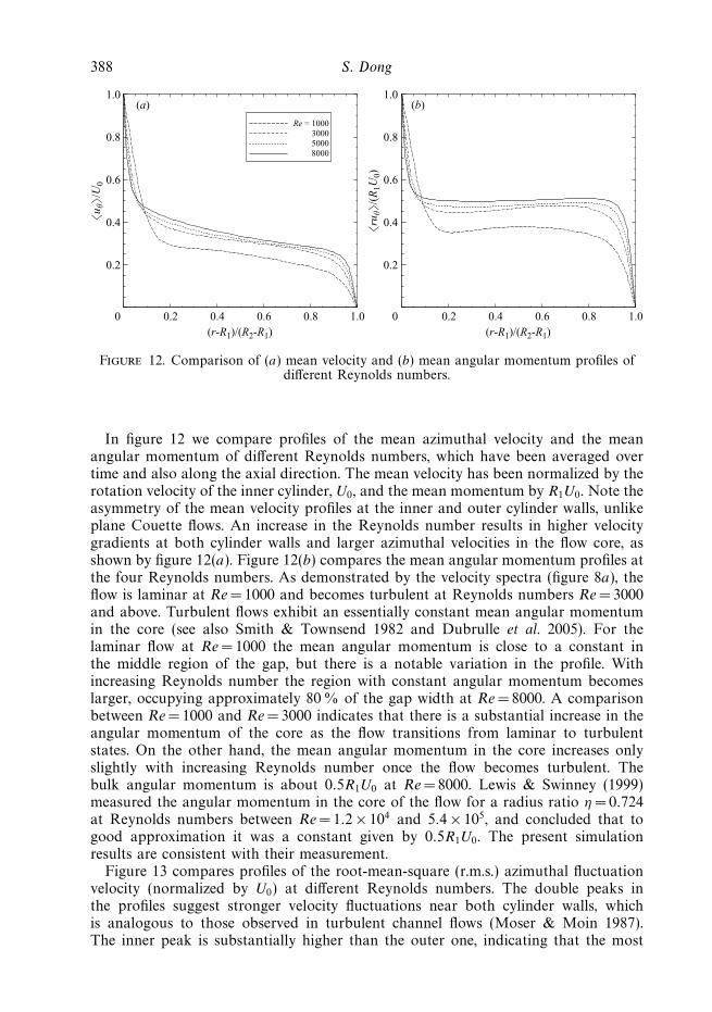
Figure 12. Comparison of (a) mean velocity and (b) mean angular momentum profiles ofdifferent Reynolds numbers.

In figure 12 we compare profiles of the mean azimuthal velocity and the meanangular momentum of different Reynolds numbers, which have been averaged overtime and also along the axial direction. The mean velocity has been normalized by therotation velocity of the inner cylinder, U0, and the mean momentum by R1U0. Note theasymmetry of the mean velocity profiles at the inner and outer cylinder walls, unlikeplane Couette flows. An increase in the Reynolds number results in higher velocitygradients at both cylinder walls and larger azimuthal velocities in the flow core, asshown by figure 12(a). Figure 12(b) compares the mean angular momentum profiles atthe four Reynolds numbers. As demonstrated by the velocity spectra (figure 8a), theflow is laminar at Re =1000 and becomes turbulent at Reynolds numbers Re= 3000and above. Turbulent flows exhibit an essentially constant mean angular momentumin the core (see also Smith & Townsend 1982 and Dubrulle et al. 2005). For thelaminar flow at Re =1000 the mean angular momentum is close to a constant inthe middle region of the gap, but there is a notable variation in the profile. Withincreasing Reynolds number the region with constant angular momentum becomeslarger, occupying approximately 80 % of the gap width at Re = 8000. A comparisonbetween Re= 1000 and Re= 3000 indicates that there is a substantial increase in theangular momentum of the core as the flow transitions from laminar to turbulentstates. On the other hand, the mean angular momentum in the core increases onlyslightly with increasing Reynolds number once the flow becomes turbulent. Thebulk angular momentum is about 0.5R1U0 at Re= 8000. Lewis & Swinney (1999)measured the angular momentum in the core of the flow for a radius ratio η = 0.724at Reynolds numbers between Re = 1.2 × 104 and 5.4 × 105, and concluded that togood approximation it was a constant given by 0.5R1U0. The present simulationresults are consistent with their measurement.

Figure 13 compares profiles of the root-mean-square (r.m.s.) azimuthal fluctuationvelocity (normalized by U0) at different Reynolds numbers. The double peaks inthe profiles suggest stronger velocity fluctuations near both cylinder walls, whichis analogous to those observed in turbulent channel flows (Moser & Moin 1987).The inner peak is substantially higher than the outer one, indicating that the most


(r-R1)/(R2-R1)

u′θ—U0

0.2 0.4 0.6 0.8 1.00

0.02

0.04

0.06

0.08

0.10

0.12

0.14

0.16Re = 1000

300050008000

Figure 13. Comparison of r.m.s. azimuthal fluctuation velocity profiles of differentReynolds numbers.

energetic turbulence occurs near the inner cylinder wall. The two peaks in the r.m.s.velocity profiles move closer to both cylinder walls with increasing Reynolds number.

5. Concluding remarksIn this paper we have studied turbulent Taylor–Couette flow at Reynolds numbers

ranging from 1000 to 8000 for a radius ratio η = 0.5 employing detailed three-dimensional direct numerical simulations. We have focused on the dynamics ofsmall-scale Gortler vortices and the herringbone-like streaks near both cylinder walls,and the statistical features of Taylor–Couette turbulence.

Barcilon et al. (1979) first reported observations of small-scale structures nearcylinder walls that formed a fine herringbone-like pattern of streaks in Taylor–Couette experiments. They conjectured that these streaks were the inflow/outflowboundaries of Gortler vortices, which were due to a centrifugal instability, occurringin a curved flow in which the local angular momentum decreased outwards alongthe radius of curvature (Saric 1994). This elementary theory was compared withexperiments, and good agreement was observed. Subsequently, Barcilon & Brindley(1984) developed a mathematical formulation to model the system of Taylor andGortler vortices hypothesized in Barcilon et al. (1979), exploiting the separation ofscales of the Taylor mode (commensurate with the gap width) and the Gortler mode(commensurate with the boundary layer thickness) and the assumption of ‘marginalstability’ (see Barcilon et al. 1979). The results of this model were shown to be in goodagreement with a number of features of experimental observations. Wei et al. (1992)critically evaluated the Gortler hypothesis of Barcilon et al. (1979) and Barcilon &Brindley (1984) with detailed experiments for a wide range of radius ratios andReynolds numbers. They noted that the radius of curvature and the velocity gradientwere the crucial parameters governing the strength of the Gortler mechanism. Thecombination of a smaller radius of curvature and a larger velocity gradient at the innercylinder (compared to the outer one) therefore suggested the emergence of Gortlervortices at the inner cylinder wall before the outer cylinder. With flow visualizations,they indeed observed that Gortler vortices appeared first at the inner cylinder wall,

390 S. Dong

and at a Taylor number an order of magnitude lower than those reported by Barcilonet al. (1979).

Results of the present simulations have confirmed the above experimentalobservations of the near-wall herringbone streaks and the onset of Gortler vorticesat the inner cylinder wall. Furthermore, the simulations have revealed additionalcharacteristics. We observe that the Gortler vortices originate around the outflowboundaries between Taylor vortex cells. In three-dimensional space these vortices aredistributed randomly in banded regions concentrating at the outflow boundaries. Withincreasing Reynolds number they spread over the entire cylinder surface, and theirconcentration around the outflow boundaries becomes less obvious. Instantaneously,a Gortler vortex appears to originate from the wall, stretch azimuthally, and extendaway from the wall.

When studying the transition to turbulence in Taylor–Couette flow, Townsend andco-workers (Smith & Townsend 1982; Townsend 1984) presented arguments that atmoderately high Reynolds numbers Gortler vortices dominated the near-wall struc-ture, and as the Reynolds number increased further the near-wall structure becamemore like that of a plane turbulent boundary layer. This implies a distinct differencebetween Gortler vortices and the structures of plane turbulent boundary layers whichare dominated by quasi-streamwise vortices near the wall (Robinson 1991; Jeonget al. 1997). Wei et al. (1992) noted that this assumption was in conflict with thework of Blackwelder (see e.g. Swearingen & Blackwelder 1987) who argued thatthe near-wall streamwise vortices found in plane turbulent boundary layers may becreated by the Gortler mechanism due to the curvature of small surface imperfectionspresent in physical experiments. The near-wall azimuthal vortices observed in thepresent simulations are not dissimilar to the near-wall streamwise vortices observedin plane turbulent channel flows. For example, both result in stronger r.m.s. velocityfluctuations (figure 13) and the streaky structures near the wall. While the near-wallstreaks in turbulent Taylor–Couette flow form herringbone patterns, the averagestreak spacing is about 100 viscous wall units (figure 10b) in both types of flows.

We summarize the main results of this study as follows:(i) Gortler vortices originate from the outflow boundaries between Taylor vortex

cells at the inner cylinder wall.(ii) In three-dimensional space Gortler vortices are randomly distributed in banded

regions on the wall, concentrating at the outflow boundaries. With increasing Reynoldsnumber these vortices spread over the entire cylinder surface.

(iii) Gortler vortices cause near-wall streaky structures that form herringbone-likepatterns. The average axial spacing of these streaks is approximately 100 viscous wallunits. The tilting angle of the streaks approximately ranges from 16 to 20 in therange of Reynolds numbers studied here.

(iv) The mean angular momentum is essentially a constant in the core of turbulentTaylor–Couette flow. The value of this constant increases slightly with increasingReynolds number in the range of turbulent Reynolds numbers in this study. It isapproximately 0.5R2

1Ω in the core at the highest Reynolds number studied here,Re= 8000.

(v) The mean velocity field reveals organized Taylor vortices underlying theturbulent Taylor–Couette flow. The instantaneous flow is a superposition of turbulentfluctuations on these organized Taylor vortices.

The author gratefully acknowledges the support from the National ScienceFoundation (NSF). Computer time was provided by the TeraGrid (TACC, NCSA,


SDSC, PSC) through an MRAC grant, and by the Rosen Center for AdvancedComputing (RCAC) at Purdue University.

REFERENCES

del Alamo, J. C., Jimenez, J., Zandonade, P. & Moser, R. D. 2006 Self-similar vortex clusters inthe turbulent logarithmic region. J. Fluid Mech. 561, 329–358.

Barcilon, A. & Brindley, J. 1984 Organized structures in turbulent Taylor-Couette flow. J. FluidMech. 143, 429–449.

Barcilon, A., Brindley, J., Lessen, M. & Mobbs, F. R. 1979 Marginal instability in Taylor-Couetteflows at a high Taylor number. J. Fluid Mech. 94, 453–463.

Barenghi, C. F. & Jones, C. A. 1989 Modulated Taylor-Couette flow. J. Fluid Mech. 208, 127–160.

Batten, W. M., Bressloff, N. W. & Turnock, S. R. 2002 Transition from vortex to wall driventurbulence production in the Taylor-Couette system with a rotating inner cylinder. IntlJ. Numer. Method Fluids 38, 207–226.

van den Berg, T. H., Doering, C. R., Lohse, D. & Lathrop, D. P. 2003 Smooth and roughboundaries in turbulent Taylor-Couette flow. Phys. Rev. E 68, 036307.

Bilgen, E. & Boulos, E. 1973 Functional dependence of torque coefficient of coaxial cylinders gapwidth and reynolds numbers. Trans. ASME: J. Fluids Engng 95, 122–126.

Bilson, M. & Bremhorst, K. 2007 Direct numerical simulation of turbulent Taylor-Couette flow.J. Fluid Mech. 579, 227–270.

Brandstater, A. & Swinney, H. L. 1987 Strange attractors in weakly turbulent Couette-Taylorflow. Phys. Rev. A 35, 2207–2220.

Cliffe, K. A. & Mullin, T. 1985 A numerical and experimental study of anomalous modes in theTaylor experiment. J. Fluid Mech. 153, 243–258.

Coles, D. 1965 Transition in circular Couette flow. J. Fluid Mech. 21, 385–425.

Coughlin, K. T. & Marcus, P. S. 1992a Modulated waves in Taylor-Couette flow Part 1. analysis.J. Fluid Mech. 234, 1–18.

Coughlin, K. T. & Marcus, P. S. 1992b Modulated waves in Taylor-Couette flow Part 2. numericalsimulation. J. Fluid Mech. 234, 19–46.

Coughlin, K. & Marcus, P. S. 1996 Turbulent bursts in Couette-Taylor flow. Phys. Rev. Lett. 77,2214–2217.

Coughlin, K. T., Marcus, P. S., Tagg, R. P. & Swinney, H. L. 1991 Distinct quasiperiodic modeswith like symmetry in a rotating fluid. Phys. Rev. Lett. 66, 1161–1164.

Czarny, O., Serre, E., Bontoux, P. & Lueptow, R. M. 2004 Interaction of wavy cylindrical Couetteflow with endwalls. Phys. Fluids 16, 1140–1148.

DiPrima, R. C. & Swinney, H. L. 1981 Instabilities and transition in flow between concentricrotating cylinders. In Hydrodynamic Instabilities and the Transition to Turbulence (ed. H. L.Swinney & J. P. Gollub) pp. 139–180. Springer.

Dong, S. & Karniadakis, G. E. 2005 DNS of flow past a stationary and oscillating cylinder atRe= 10000. J. Fluids Struct. 20, 519–531.

Dong, S., Karniadakis, G. E., Ekmekci, A. & Rockwell, D. 2006 A combined direct numericalsimulation-particle image velocimetry study of the turbulent near wake. J. Fluid Mech. 569,185–207.

Donnelly, R. J. & Simon, N. J. 1959 An empirical torque relation for supercritical flow betweenrotating cylinders. J. Fluid Mech. 7, 401–418.

Dubrulle, B., Dauchot, O., Daviaud, F., Longaretti, P.-Y., Richard, D. & Zahn, J.-P. 2005Stability and turbulent transport in Taylor-Couette flow from analysis of experimental data.Phys. Fluids 17, 095103.

Fasel, H. & Booz, O. 1984 Numerical investigation of supercritical Taylor-vortex flow for a widegap. J. Fluid Mech. 138, 21–52.

Fernstermatcher, P. R., Swinney, H. L. & Gollub, J. P. 1979 Dynamical instabilities and thetransition to chaotic Taylor vortex flow. J. Fluid Mech. 94, 103–128.

Gortler, H. 1954 On the three-dimensional instability of laminar boundary layers on concavewalls. NACA TM 1375.

Jeong, J. & Hussain, F. 1995 On the identification of a vortex. J. Fluid Mech. 285, 69–94.

392 S. Dong

Jeong, J., Hussain, F., Schoppa, W. & Kim, J. 1997 Coherent structures near the wall in a turbulentchannel flow. J. Fluid Mech. 332, 185–214.

Jones, C. A. 1981 Nonlinear Taylor vortices and their stability. J. Fluid Mech. 102, 249–261.

Jones, C. A. 1982 On flow between counter-rotating cylinders. J. Fluid Mech. 120, 433–450.

Jones, C. A. 1985 The transition to wavy Taylor vortices. J. Fluid Mech. 157, 135–162.

Karniadakis, G. E., Israeli, M. & Orszag, S. A. 1991 High-order splitting methods for theincompressible Navier-Stokes equations. J. Comput. Phys. 97, 414–443.

Karniadakis, G. E. & Sherwin, S. J. 2005 Spectral/hp Element Methods for Computational FluidDynamics , 2nd edn. Oxford University Press.

Kim, J., Moin, P. & Moser, R. 1987 Turbulent staistics in fully-developed channel flow at lowreynolds-number. J. Fluid Mech. 177, 133–166.

King, G. P., Li, Y., Lee, W., Swiney, H. L. & Marcus, P. S. 1984 Wave speeds in wavy Taylor-vortexflow. J. Fluid Mech. 141, 365–390.

Kirby, R. M. & Karniadakis, G. E. 2003 De-aliasing on non-uniform grids: algorithms andapplications. J. Comput. Phys. 91, 249–264.

Kline, S. J., Reynolds, W.C., Schraub, F. A. & Runstadler, P. W. 1967 The structure of turbulentboundary layers. J. Fluid Mech. 30, 741.

Koschmieder, E. L. 1979 Turbulent Taylor vortex flow. J. Fluid Mech. 93, 515–527.

Lathrop, D. P., Fineberg, J. & Swinney, H. L. 1992a Transition to shear-driven turbulence inCouette-Taylor flow. Phys. Rev. A 46, 6390–6405.

Lathrop, D. P., Fineberg, J. & Swinney, H. L. 1992b Turbulent flow between concentric rotatingcylinders at large reynolds number. Phys. Rev. Lett. 68, 1515–1518.

Lewis, G. S. & Swinney, H. L. 1999 Velocity structure functions, scaling, and transitions inhigh-Reynolds-number Couette-Taylor flow. Phys. Rev. E 59, 5457–5467.

Marcus, P. S. 1984a Simulation of Taylor-Couette flow. Part 1. numerical methods and comparisonwith experiment. J. Fluid Mech. 146, 45–64.

Marcus, P. S. 1984b Simulation of Taylor-Couette flow. Part 2. numerical results for wavy-vortexflow with one travelling wave. J. Fluid Mech. 146, 65–113.

Moser, R. D. & Moin, P. 1987 The effects of curvature in wall-bounded turbulent flows. J. FluidMech. 175, 479–510.

Moulic, S. G. & Yao, L. S. 1996 Taylor-Couette instability of travelling waves with a continuousspectrum. J. Fluid Mech. 324, 181–198.

Mujumdar, A. K. & Spalding, D. B. 1977 Numerical computation of Taylor vortices. J. FluidMech. 81, 295–304.

Parker, J. & Merati, P. 1996 An investigation of turbulent Taylor-Couette flow using laser Dopplervelocimetry in a refractive index matched facility. Trans. ASME: J. Fluids Engng 118, 810–818.

Racina, A. & Kind, M. 2006 Specific power and local micromixing times in turbulenct Taylor-Couette flow. Exps. Fluids 41, 513–522.

Rashidi, M. & Banerjee, S. 1990 The effect of boundary conditions and shear rate on streakformation and breakdown in turbulent channel flows. Phys. Fluids A 2, 1827–1838.

Riechelmann, D. & Nanbu, K. 1997 Three-dimensional simulation of wavy Taylor vortex flow bydirect simulation Monte Carlo method. Phys. Fluids 9, 811–813.

Rigopoulos, J., Sheridan, J. & Thompson, M. C. 2003 State selection in Taylor-Couette flowreached with an accelerated inner cylinder. J. Fluid Mech. 489, 79–99.

Robinson, S. K. 1991 Coherent motions in the turbulent boundary layer. Annu. Rev. Fluid Mech.23, 601.

Saric, W. S. 1994 Gortler vortices. Annu. Rev. Fluid Mech. 26, 379–409.

She, Z.-S., Ren, K., Lewis, G. S. & Swinney, H. L. 2001 Scalings and structures in turbulentCouette-Taylor flow. Phys. Rev. E 64, 016308.

Smith, C. R. & Metzler, S. P. 1983 The characteristics of low-speed streaks in the near-wall regionof a turbulent boundary layer. J. Fluid Mech. 129, 27–54.

Smith, G. P. & Townsend, A. A. 1982 Turbulent Couette flow between concentric cylinders at largeTaylor numbers. J. Fluid Mech. 123, 187–217.

von Stamm, J., Gerdts, U., Buzug, T. & Pfister, G. 1996 Symmetry breaking and period doublingon a torus in the VLF regime in Taylor-Couette flow. Phys. Rev. E 54, 4938–4957.


Swearingen, J. D. & Blackwelder, R. F. 1987 The growth and breakdown of streamwise vorticesin the presence of a wall. J. Fluid Mech. 182, 255.

Takeda, Y. 1999 Quasi-periodic state and transition to turbulence in a rotating Couette system.J. Fluid Mech. 389, 81–99.

Tam, W. Y. & Swinney, H. L. 1987 Mass transport in turbulent Couette-Taylor flow. Phys. Rev. A36, 1374–1381.

Taylor, G.I. 1923 Stability of a viscous liquid contained between two rotating cylinders. Phil. Trans.R. Soc. Lond. A 223, 289.

Tong, P., Goldburg, W. I., Huang, J. S. & Witten, T. A. 1990 Anisotropy in turbulent dragreduction. Phys. Rev. Lett. 65, 2780–2783.

Townsend, A. A. 1984 Axisymmetric Couette flow at large Taylor numbers. J. Fluid Mech. 144,329–362.

Vastano, J. A. & Moser, R. D. 1991 Short-time Lyapunov exponent analysis and the transition tochaos in Taylor-Couette flow. J. Fluid Mech. 233, 83–118.

Wei, T., Kline, E. M., Lee, S. H. K. & Woodruff, S. 1992 Gortler vortex formation at the innercylinder in Taylor-Couette flow. J. Fluid Mech. 245, 47–68.

Wendt, F. 1933 Turbulente stromungen zwischen zwei eorierenden konaxialen zylindem. Ing.-Arch.4, 577–595.

Wild, P. M., Djilali, N. & Vickers, G. W. 1996 Experimental and computational assessment ofwindage losses in rotating machinery. Trans. ASME: J. Fluids Engng 118, 116–122.

direct numerical simulation of turbulent taylor–couette flow

Documents