HAL Id: hal-01969425https://hal.archives-ouvertes.fr/hal-01969425

Submitted on 4 Jan 2019

HAL is a multi-disciplinary open accessarchive for the deposit and dissemination of sci-entific research documents, whether they are pub-lished or not. The documents may come fromteaching and research institutions in France orabroad, or from public or private research centers.

L’archive ouverte pluridisciplinaire HAL, estdestinée au dépôt et à la diffusion de documentsscientifiques de niveau recherche, publiés ou non,émanant des établissements d’enseignement et derecherche français ou étrangers, des laboratoirespublics ou privés.

Direct or indirect on-shore hydrocarbon detectionmethods applied to hyperspectral data in tropical areaVéronique Achard, Sophie Fabre, Alexandre Alakian, Dominique Dubucq,

Philippe Déliot

To cite this version:Véronique Achard, Sophie Fabre, Alexandre Alakian, Dominique Dubucq, Philippe Déliot. Direct orindirect on-shore hydrocarbon detection methods applied to hyperspectral data in tropical area. SPIERemote Sensing, Sep 2018, BERLIN, Germany. �10.1117/12.2325097�. �hal-01969425�

Direct or indirect on-shore hydrocarbon detection methods applied to hyperspectral data in tropical area

Véronique Acharda, Sophie Fabrea, Alexandre Alakianb, Dominique Dubucqc, Philippe Déliota, a,bONERA “The French Aerospace Lab”, a2 Av. ´ Edouard Belin, 31000 Toulouse, France and

b28 chemin de la Hunière et des Joncherettes , 91120 Palaiseau, France cTOTAL, avenue Larribau, 64000 Pau, France

ABSTRACT

Detecting onshore hydrocarbon is a major topic for both environmental monitoring and exploration. In this work, a hyperspectral image acquired nearby an old oil extraction site in tropical area is analyzed. The area of interest includes a pit filled with bio-degraded heavy oil, surrounded by herbaceous vegetation and many lagoons.

First, we focused on methodologies that can detect oil pollution in an unsupervised manner. Based on the assumption that such oil pits are rare events in the image, statistical approach for anomalies detection, derived from the Reed-Xiaoli detector, is used. In order to decrease the number false alarms, some a priori knowledge about the spectral signature of the pits and about the background is introduced. This approach succeeds in detecting the pit with very few false alarms.

Hydrocarbon pollution can have an impact on vegetation and leads to change in vegetation (bio)physical parameters (pigments, water content, …), according to species, pollutant type and exposition time . In order to map the polluted area without any a priori knowledge, several un-supervised classification, including an original method of automatic classification combining unmixing approach and SVM (support Vector Machine) are applied and compared. The results are compared with a partial “ground truth map” that has been derived from visual observations on the field, and with areas of stressed vegetation that have been mapped using combination of specific spectral indices. The classification results are consistent with the ground truth map and the retrieved stressed vegetation areas.

Keywords: Hyperspectral, Hydrocarbon detection, Spectral unmixing, Unsupervised classification, Anomaly detection, spectral index.

1. INTRODUCTION

Although oil is an important source of energy and is used in the composition of many manufactured products, its extraction and transport can cause more or less episodic pollution. It is therefore essential to have observation means and associated processing tools to detect this pollution and to monitor potentially polluted areas. For this issue, the potentiality of hyperspectral images, providing the ability to make distinctions among materials with only subtle spectral signature differences, is studied. Cloutis (1989) [1] has demonstrated that hydrocarbon-bearing reference objects are characterized by absorption maxima at 1.73 µm and 2.31 µm. Horig et al. (2001) [2] proved the possibility of highlighting the presence of hydrocarbons mixed with sand and plastic materials on a HyMap image, thanks to these specific absorption bands. In 2004 Kuhn et al. [3] defined a hydrocarbon index using the 1.73 µm absorption band in order to detect automatically these materials on the HyMap image. After the Deep Water Horizon accident, Kokaly et al. [4], [5] was able to map the oil-impacted coastal areas, using MICA software (Material Identification and Characterization Algorithm), which uses the Tetracorder spectral feature matching algorithm [6]. The authors compared spectral feature observed on field measurements (1.73 µm and 2.31 µm for oil detection) and AVIRIS spectra. In [7] coastal pollution has been mapped using linear unmixing techniques. Endmembers are extracted from Aviris images using PPI (Purity Pixel Index (ENVI®), followed by the selection of the purest pixels with the N-D Visualizer (ENVI®). Then Multiple Endmember Spectral Mixture Analysis (MESMA) is applied to map the abundances of these endmembers. In this work, the area of interest is an former oil extraction site that has been flown over with two HySpex Hyperspectral cameras, one covering the VNIR spectral range (0.4 µm-1 µm) and the other, the SWIR spectral range (1µm -2.5 µm). In this area is located a tar pit, surrounded by stressed or sparse vegetation. For old bio-degraded oil, the specific hydrocarbon features at 1.73 µm and 2.3 µm tend to disappear, that makes detection from these features impossible.

More, heavy oil which is characterized by low reflectance values can be easily confused with other dark materials or shade. The first part of this paper is dedicated to the methodology we propose for the detection of such former oil pits. In the second part, unsupervised classification methods are applied, in order to give an overview of the polluted area, in the context in which no prior information is available about the scene. Several classification schemes based on spectral unmixing are proposed and compared to K-means.

2. MATERIALS

2.1 Image acquisition and pre-processing

Hyperspectral images were acquired in June 2015 at a former oil exploration site in tropical zone, using two HySpex cameras from NEO (Norsk Elektro Optikk) [8], a VNIR1600 and a SWIR320m-e which have respectively 160 spectral bands in the VNIR domain [0:4 µm- 1:0 µm] and 256 bands in the SWIR domain [1.0 µm -2.5 µm]. The ground sample distance was 1.3 m for the VNIR data and 2.6 m for the SWIR data. The radiometric correction was performed using NEO software and was followed by a correction of the aircraft window transmission. Radiance images were then corrected from atmospheric and environment effects using COCHISE [9], which is based on the use of hyperspectral information combined with the radiative transfer code MODTRAN [10]. The reference data uses for the ortho-rectification is a SPOT image with 0.65 m spatial resolution. The VNIR data is registered with the reference data and the VNIR and SWIR images were registered using GeFolki [11][12] using a nearest neighbor resampling filter to preserve spectral information. After this orthorectification stage, the spatial resolution of the VNIR-SWIR hypercube is 0.65 m. The subset of 561 x 948 pixels used in this study is shown on Figure 1. To focus on the area of interest, a mask has been built. Some pixels that have inconsistent spectral reflectance between VNIR and SWIR, due to the fact that VNIR and SWIR cameras do not have the same spatial sampling, have also been masked. These spectra can exhibit a jump between the VNIR and the SWIR bands around 1 µm. In order to limit the impact of these pixels on the future processing, those having a reflectance jump higher that 0.1 are masked. Finally it remains 380595 unmasked pixels. 2.2 Reference map

A ground truth campaign was conducted one year after the hyperspectral acquisitions during the same season to place it under the conditions which are the most similar to the image acquisition in term of vegetation phenology. From visual observation and GPS locations, some regions of interests have been manually annotated on the hysperspectral data. The regions thus identified have been extended using similarity measure based on spectral angle with a very restrictive threshold (1° spectral angle). The resulting ground truth is shown on Figure 1.

Figure 1. From left to right: RGB image extracted from the HySpex hypercube, ground truth extended using similarity measurements.

3. TAR PIT DETECTION

The first objective of this work was to detect the farmer tar pit. Approaches based on hydrocarbon spectral features at 1.73 µm and 2.3 µm are not possible because they are not visible on the spectra extracted on the pit (see Figure 3(a)). Nonetheless the pit might be distinguishable from the background due to its global spectral shape. As tar pits are rare events in the scene, we applied anomaly detection methodology with some prior knowledge on the pit. Many types of anomaly detectors (ADs) have been proposed in literature [13]. The most frequently used is the Reed-Xiaoli (RX) detector [14] that is often used as a benchmark to which other methods are compared. The RX detector characterizes the background by its spectral mean �� and covariance matrix ��. The actual detector calculates the Mahalanobis distance between the pixel under test r and the background. In this work, we use a Class-conditional version of RX (CRX) [15]. In CRX, the image is first segmented and the covariance matrix and mean spectrum within each class i (i.e. ��,� and ��,�) are determined. The Mahalanobis distance between the pixel under test, r, and each of the classes is calculated. The final result is the minimum of these distances:

���� � min� ��� � ��,��� ��,����� � ��,���

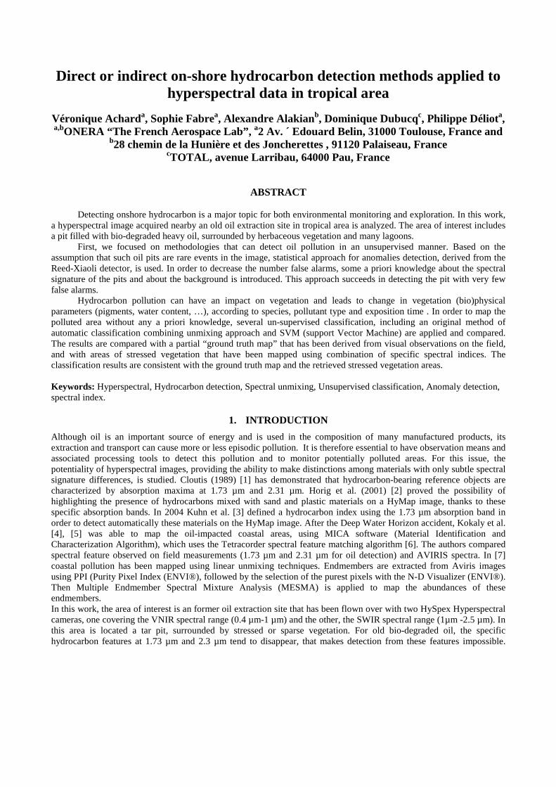
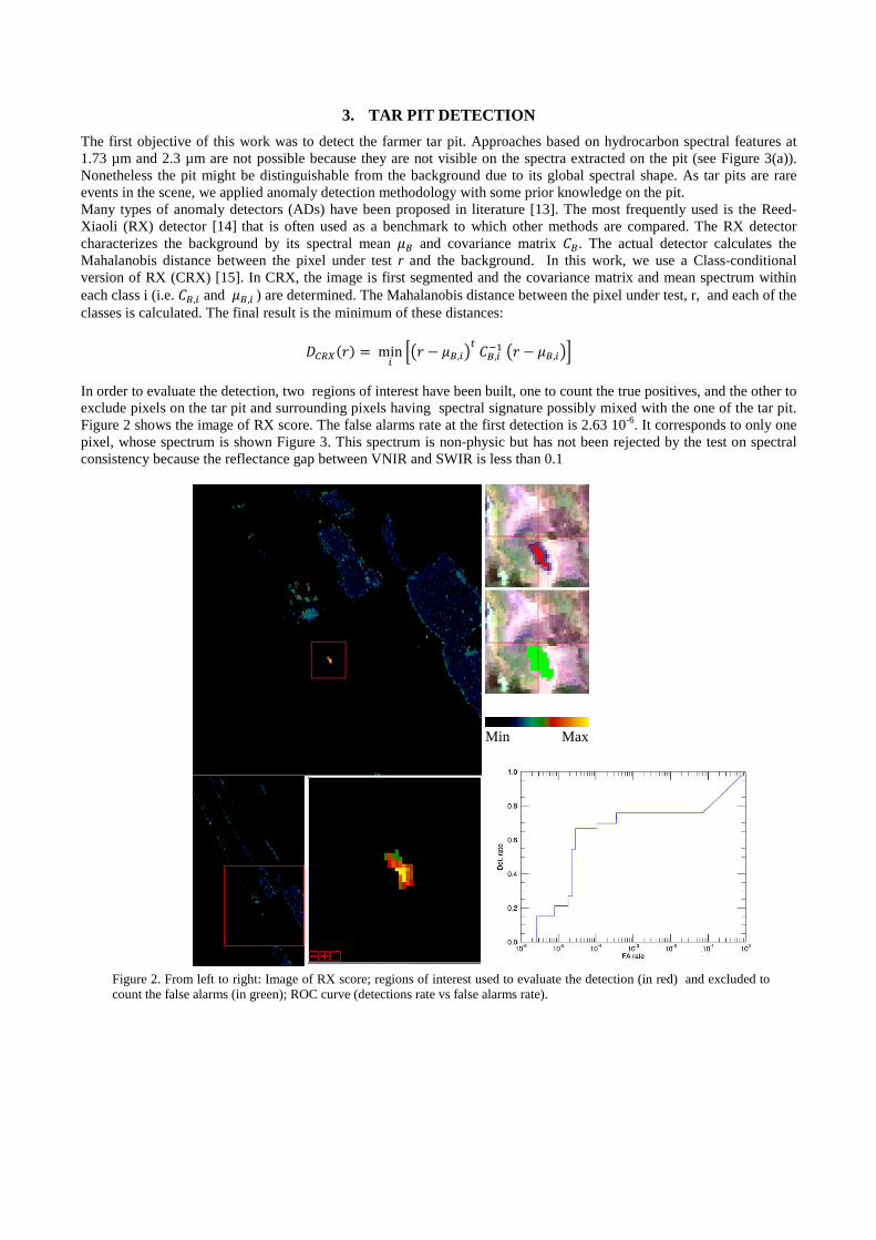
In order to evaluate the detection, two regions of interest have been built, one to count the true positives, and the other to exclude pixels on the tar pit and surrounding pixels having spectral signature possibly mixed with the one of the tar pit. Figure 2 shows the image of RX score. The false alarms rate at the first detection is 2.63 10-6. It corresponds to only one pixel, whose spectrum is shown Figure 3. This spectrum is non-physic but has not been rejected by the test on spectral consistency because the reflectance gap between VNIR and SWIR is less than 0.1

Min Max

Figure 2. From left to right: Image of RX score; regions of interest used to evaluate the detection (in red) and excluded to count the false alarms (in green); ROC curve (detections rate vs false alarms rate).

(a)

(b)

Figure 3. (a): spectral statistics of the tar pit; (b): reflectance spectrum of the false positive. On (b) the two parts of the spectrum [0.4 µm, 1 µm] and [1 µm, 2.4 µm] do not correspond to the same material, owing to the registration impact of the VNIR and SWIR images.

4. UNSUPERVISED CLASSIFICATION

The aim of this work is to get an overview of the area of interest without any prior information. For that, we tested several unsupervised classification schemes, that could be followed by a characterization step of the classes thus obtained. For instance, identifying stressed vegetation classes is particularly interesting, as they can be related by pollution in the subsurface. A common unsupervised classification method is the K-means, which assigns, at each iteration, pixels to classes according to their similarity with class centroids that are re-calculated at each iteration. In the present work, two similarity distances are used, the Euclidian distance, and the spectral angle cosine. We proposed also a new classification scheme coupling endmembers extraction, linear unmixing and SVM (Support Vector Machine). Our choice is motivated on the one hand, because linear unmixing is the powerful tool to analyze hyperspectral image. But the analysis of each abundance map can by tedious and time consuming when the number of endmembers increases. A straightforward way to classify image using abundance maps could be to assign pixels to the class for which abundance is highest. But this method gives poor results as it will be shown in the section 6. On the other hand, SVM is very efficient to classify hyperspectral data [16], but it is a supervised method that needs training samples, that are supposed unavailable in this study. The method developed in this work, named UM-SVM, uses unmixing in order to extract training samples and SVM to classify the image, which allows non-linear class boundaries. 4.1 Endmembers extraction and unmixing

We assume that the spectrum of each pixel can be well approximated by a linear mixture of the pure component spectra present in the image weighted by their fractional abundances in the pixel:

��� =∑ ��� ��!�"# $%��&. (.) * �� * #& ∑ ��!

�"# � # (1)

Where pij is the radiance or the reflectance of the pixel j in the band i, and eik is the radiance (or reflectance) of the endmember k in the band i, akj is the abundance of the endmember k in the pixel j, and wij is a residual error.

In this study an automatic endmembers extraction (AEE) is applied using a deterministic approach based on OSP (Orthogonal Subspace projection) [17]. Abundances are then computed with fully constrained unmixing method, i.e. under the positivity and sum to one constraints of Eq. (1). In unmixing process, determining the number of endmembers (EM) is a complex issue that has motivated several works [18][19]. The advantage of OSP AEE is that increasing the EM numbers do not change the EM already extracted, and thus is less sensitive to the number of EM. 4.2 Training Samples extraction and classification step

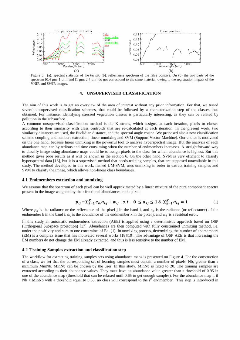
The workflow for extracting training samples sets using abundance maps is presented on Figure 4. For the construction of a class, we set that the corresponding set of learning samples must contain a number of pixels, Nb, greater than a minimum MinNb. MinNb can be chosen by the user. In this study, MinNb is fixed to 20. The training samples are extracted according to their abundance values. They must have an abundance value greater than a threshold of 0.95 in one of the abundance map (threshold that can be relaxed until 0.65 to get enough samples). For the abundance map i, if Nb < MinNb with a threshold equal to 0.65, no class will correspond to the ith endmember. This step is introduced in

order to avoid having many marginal classes. If the sample number of one class is greater than 100, a random draw is realized to balance the numbers of samples in all the classes. SVM is applied on the image using the training samples thus extracted. A polynomial kernel of degree 3 is used.

Figure 4. Construction of learning samples from the abundance maps

5. STRESSED VEGETATION MAPPING

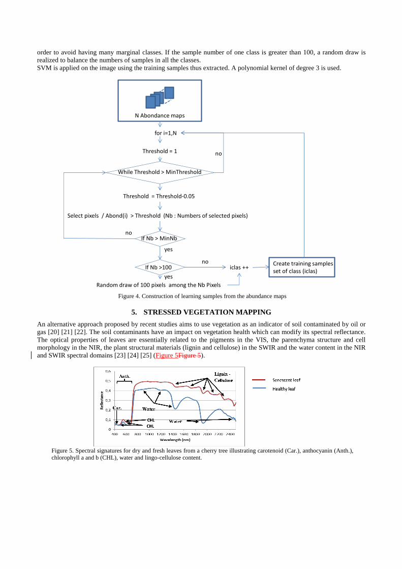
An alternative approach proposed by recent studies aims to use vegetation as an indicator of soil contaminated by oil or gas [20] [21] [22]. The soil contaminants have an impact on vegetation health which can modify its spectral reflectance. The optical properties of leaves are essentially related to the pigments in the VIS, the parenchyma structure and cell morphology in the NIR, the plant structural materials (lignin and cellulose) in the SWIR and the water content in the NIR and SWIR spectral domains [23] [24] [25] (Figure 5Figure 5).

Figure 5. Spectral signatures for dry and fresh leaves from a cherry tree illustrating carotenoid (Car.), anthocyanin (Anth.), chlorophyll a and b (CHL), water and lingo-cellulose content.

for i=1,N

Threshold = 1

While Threshold > MinThreshold

Threshold = Threshold-0.05

Select pixels / Abond(i) > Threshold (Nb : Numbers of selected pixels)

If Nb > MinNb

If Nb >100

Random draw of 100 pixels among the Nb Pixels

iclas ++

N Abondance maps

Create training samples

set of class (iclas)

yes

yes

no

no

no

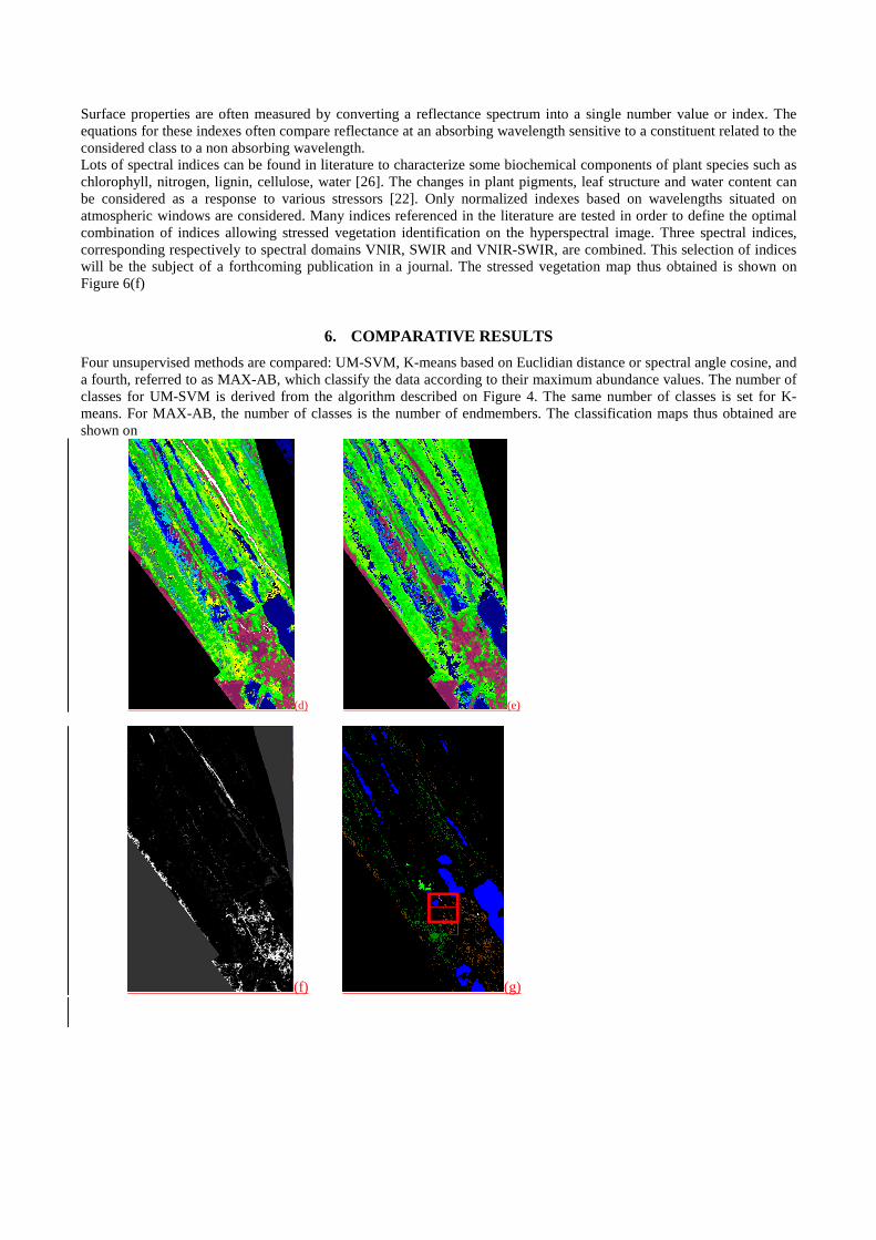
Surface properties are often measured by converting a reflectance spectrum into a single number value or index. The equations for these indexes often compare reflectance at an absorbing wavelength sensitive to a constituent related to the considered class to a non absorbing wavelength. Lots of spectral indices can be found in literature to characterize some biochemical components of plant species such as chlorophyll, nitrogen, lignin, cellulose, water [26]. The changes in plant pigments, leaf structure and water content can be considered as a response to various stressors [22]. Only normalized indexes based on wavelengths situated on atmospheric windows are considered. Many indices referenced in the literature are tested in order to define the optimal combination of indices allowing stressed vegetation identification on the hyperspectral image. Three spectral indices, corresponding respectively to spectral domains VNIR, SWIR and VNIR-SWIR, are combined. This selection of indices will be the subject of a forthcoming publication in a journal. The stressed vegetation map thus obtained is shown on Figure 6(f)

6. COMPARATIVE RESULTS

Four unsupervised methods are compared: UM-SVM, K-means based on Euclidian distance or spectral angle cosine, and a fourth, referred to as MAX-AB, which classify the data according to their maximum abundance values. The number of classes for UM-SVM is derived from the algorithm described on Figure 4. The same number of classes is set for K-means. For MAX-AB, the number of classes is the number of endmembers. The classification maps thus obtained are shown on

(d) (e)

(f) (g)

Figure 6 Figure 6. It is not easy to compare unsupervised classification results, and assign similar colors to all, because classes are not labeled. Nevertheless, we try to assign about the same colors scheme for all classification maps. More, computing confusing matrix based on the partial ground truth (GT) is not appropriate, first because the number of classes is greater than the number of GT classes and because the classes can differ from a classification method to another. The three first maps in

(d) (e)

(f) (g)

Figure 6 Figure 6 are based on endmembers extraction. (a) is UM-SVM, (b) is MAX-AB and (c) is MAX-AB where only pixels having one abundance value greater or equal to 0.65 (denoted MAX-AB65), the same threshold used in UM-SVM, are classified. First, we can notice that few pixels are classified with MAX-AB65. Only water classes have numerous pixels. Vegetation classes are poorly represented, which means that vegetation spectra in the image are modelled by a mixture (following Eq. (1)) of several endmembers extracted using, and very few pixels have a prevailing abundance that corresponds to one of the vegetation endmembers. If no threshold is put on the abundances (method MAX-AB), water classes (various blue colors) spread a lot to the detriment of vegetation classes (various green and yellow colors). Only the “stressed vegetation - bare soil+stressed vegetation” (in various maroon colors) is in good agreement with the GT. Among these three methods, only UM-SVM gives satisfying results that will be discussed in more details. This shows the interest of using SVM to classify the image from abundance maps.

The results of the K-means classification using Euclidian distance (ED) and the spectral angle (SAM) are shown respectively on

(d) (e)

(f) (g)

Figure 6 Figure 6 (d) and (e). With SAM, some vegetation area are identified as water (for instance light green class of the GT map which corresponds to yellow classes obtained with ED et UM-SVM). More the bare soil path is not identified with SAM. For these reasons, only results obtained with ED will be discussed in more details. The average spectra of each class are plotted on Figure 7 keeping the same colors as those of the classification maps. Line (a) is UM-SVM and line (b) K-means-ED. The average spectra of the ground truth are on line (c). This figure shows also the distribution of the pixels of the different GT classes in the classes obtained by UM-SVM or K-means. A class related to the path, that is not present in the partial ground truth is identified by UM-SVM (class 8) and K-means (class 3). Class 2 of UM-SVM corresponds to green and dense vegetation, which is not identified by K-means, and not present in the GT. Neither method identifies the tar pit. The corresponding pixels are included in one of the water classes. Generally speaking we note that a GT class is split into more K-means classes than into UM-SVM classes. The spectral differences between average spectra associated to the K-means are significantly smaller than those of UM-SVM. For UM-SVM, spectra of class 9 and 10 are quite similar to those of class 5 and class 3, respectively, that explains to spreading of dark green and light green GT classes, in one hand, and of the brown and dark green GT classes on the other hand, into these pairs of UM-SVM classes. The deepest water class, which has the lowest reflectance spectra, is better identified by K-means that UM-SVM, which leads to a class that has only deep water pixels (class 1), unlike UM-SVM. The reverse is observed for the edge of ponds.

In conclusion, UM-SVM method retrieves more relevant classes than K-means, with an additional advantage that the number of classes is determined by the method, unlike K-means for which the number of classes must be fixed in a more or less arbitrary way by the user. Both methods identify classes coinciding with areas of interest such as stressed vegetation, which may be an indicator of oil pollution.

(a) (b) (c)

(d) (e)

(f) (g)

Figure 6. Classification maps obtained with UM-SVM (a), MAX-AB(b), MAX-AB65 (c), K-means-ED (d), K-means-SAM (e), Stressed vegetation reference map (f) and GT extended using spectral angle with 1° threshold (g).

(a)

(b)

(c)

Figure 7 – Average spectra of each class obtained with UM-SVM (top), K-means-ED (b) and GT (c). Beside, the distribution of GT pixels into classes, and the distribution of stressed vegetation into classes are shown for the two classification methods

The Figure 6(f) Figure 6presents the stressed vegetation map (in white) resulting from the combination of the spectral indices described in the previous section (§ 5). Stressed vegetation areas are located around the pit and near a path. These areas are consistent with field observations. Stressed Vegetation is also present at other locations on the image, where no field information is available. Promising perspectives for hydrocarbon detection applications according to impact on vegetation stress are then suggested.

7. CONCLUSION

The objective of this study was to analyze an area close to a former oil exploitation site, without prior knowledge of the terrain, but certainly affected by oil pollution, which we are trying to highlight on the hyperspectral image. First anomaly detection has been applied in order to detect the presence of tar pits. The RX-Cluster method has been applied, with some assumptions to reduce the false alarms occurrences: a NDVI test has been added to reject vegetation pixels and a reflectance level test to focus detection on objects with low reflectance. With this approach, the tar pit present in the image is detected with only one false alarm. Then unsupervised classification methods have be applied in order to obtain an overall mapping of the area. The classes thus obtained could be identified a posteriori. Among the tested methods, the K-means method, using Euclidian distance, and a new method, UM-SVM, coupling unmixing and SVM, give good results, in accordance with a partial ground truth map, that was based on in-situ observations. The advantage of UM-SVM is to give more differentiated classes, while average spectra the K-means classes are much more similar. But both the methods succeeds in retrieving classes of particular interest such as stressed vegetation as it can be related to oil pollution for monitoring soil contamination in densely vegetated oil and gas exploration and production regions.

REFERENCES

[1] Cloutis, E. A., “Spectral reflectance properties of hydrocarbons: remote sensing implications”. Science, 245, 165–168, Jul. 1989.

[2] Hörig, B. F. Kühn , F. Oschütz & F. Lehmann, “HyMap hyperspectral remote sensing to detect hydrocarbons”. International Journal of Remote Sensing, 1413-1422, (2001)

[3] Kühn, F. “Hydrocarbon Index - An algorithm for hyperspectral detection of hydrocarbons”. International Journal of Remote Sensing - INT J REMOTE SENS. 25, 2467-2473, (2004).

[4] Kokaly, R. F.. “Shoreline surveys of oil-impacted marsh in southern Louisiana”. U.S. geological survey open-file report, (2011)

[5] Kokaly, R. F. (2013). “Spectroscopic remote sensing of the distribution and persistence of oil from the Deepwater Horizon spill in Barataria Bay marshes”. Remote Sensing of Environment, 129, 210-230

[6] Clark, R. N., Swayze, G.A., Livo, K.E., Kokaly, R.F., Sutley, S.J., Dalton, J.B., McDougal, R.R., and Gent, C.A., “Imaging spectroscopy: Earth and planetary remote sensing with the USGS Tetracorder and expert systems”, Journal of Geophysical Research, Vol. 108(E12), 5131, doi:10.1029/2002JE001847, p. 5-1 to 5-44, December, (2003). http://speclab.cr.usgs.gov/PAPERS/tetracorder

[7] Arslan, M. D. (2013). “Oil Spill Detection and Mapping Along the Gulf of Mexico Coastline Based on Imaging Spectrometer Data”. Texas: Texas A & M University.

[8] HySpex Hyperspectral Cameras – Norsk Elektro Optikk, http://www.hyspex.no/products/. [9] Miesch, C. P., L. Poutier, V. Achard, X. Briottet, X. Lenot, Y. Boucher, “Direct and inverse radiative transfer

solutions for visible and near-infrared hyperspectral imagery”. IEEE Trans. Geosc. Remote Sensing, vol. 43, n°7, 1552-1562 (2005).

[10] Berk A., G. P. Anderson, L. S. Bernstein, et al., “MODTRAN4 radiative transfer modeling for atmospheric correction,” vol. 3756, International Society for Optics and Photonics, Oct. 1999, pp. 348–354, (1999)

[11] Plyer, A. E. Colin-Koeniguer, and F. Weissgerber, “A new coregistration algorithm for recent applications on urban sar images,” IEEE Geosci. Remote Sens. Lett., vol. 12, no. 11, pp. 2198–2202, Nov. 2015

[12] Brigot, G., Colin-Koeniguer, E., Plyer, A., Janez, F. “Adaptation and Evaluation of an optical flow method applied to co-registration of forest remote sensing images”, IEEE Journal of Selected Topics in Applied Earth Observations and Remote Sensing, Volume: 9, Issue7, July 2016, (2016) http://w3.onera.fr/medusa/gefolki

[13] Matteoli, S., Diani, M., and Corsini, G., “A tutorial overview of anomaly detection in hyperspectral imagery”, IEEE A&S Systems Magazine, Part3: Tutorials 21 (June 2010).

[14] Reed, I.S. and Yu, X., “Adaptive multiband cfar detection of an optical pattern with unknown spectral distribution,” IEEE ASSP 38, 1760–1770 (Oct 1990).

[15] Borghys D., I. Kasen, V. Achard, C. Perneel, “Hyperspectral anomaly detection: Comparative evaluation in s cenes with diverse complexity”, Journal of Electrical and Computer Engineering, Special Issue on "Algorithms for Multispectral and Hyperspectral Image Analysis, 2012

[16] Gualtieri J. A., S. R. Chettri, R. F. Cromp, "Support vector machines for hyperspectral remote sensing classification", Proc. of the SPIE, vol. 3584, pp. 221-232, (1999)

[17] Chang, C., “Orthogonal subspace projection (OSP) revisited: a comprehensive study and analysis”. IEEE Trans. on Geoscience and Remote Sensing, vol. 43, no. 3, 502-518, (2005)

[18] Bioucas-Dias, J. M. and Nascimento J. M., “Hyperspectral Subspace Identification”, IEEE Trans. Geoscience and Remote Sensing, vol: 46, issue 8 (2008 )

[19] Luo B. and J. Chanussot, “Unsupervised classification of hyperspectral images by using linear unmixing algorithm”, 16th IEEE International Conference on Image Processing (ICIP) (2009)

[20] Noomen, M. F., van der Werff, H. M. A., van der Meer, F. D., “Spectral and spatial indicators of botanical changes caused by long-term hydrocarbon seepage”. Ecol. Inform. 2012, 8, 55−64.

[21] Arellano, P., Tansey, K., Balzter, H., Boyd, D. S. “Detecting the effects of hydrocarbon pollution in the Amazon forest using hyperspectral satellite images”. Environ. Pollut. 2015, 205, 225−239.

[22] Lassalle, G., A. Credoz,, R. Hédacq, S. Fabre, D. Dubucq, A. Elger, "Assessing soil contamination from oil and gas production using vegetation hyperspectral reflectance", Environmental Science & Technology, 2018 Feb 20;52(4):1756-1764.

[23] Sims, D. A.; Gamon, J. A. “Relationships between leaf pigment content and spectral reflectance across a wide range of species, leaf structures and developmental stages”. Remote Sens. Environ. 2002, 81, 337−354.

[24] Ustin, S. L., A. A. Gitelson, S. Jacquemoud, M. Schaepman, G.P. Asner, J. A. Gamon, P. Zarco-Tejada, “Retrieval of foliar information about plant pigment systems from high resolution spectroscopy”, Remote Sensing of Environment 113, Supplement 1 (September 2009; Imaging Spectroscopy Special Issue), pp. S67–S77; doi: 10.1016/j.rse.2008.10.019

[25] Cheng, Y. B., P. J. Zarco-Tejada, D. Riaño, C. A. Rueda, S. L.Ustin, “Estimating vegetation water content with hyperspectral data for different canopy scenarios: Relationships between AVIRIS and MODIS indexes”, Remote Sensing of Environment, Volume 105, Issue 4, 30 December 2006, Pages 354-366

[26] Erudel, T., S. Fabre, T. Houet, F. Mazier, X. Briottet, “Criteria comparison for classifying peatland vegetation types using in situ hyperspectral measurements”, Remote Sensing, 2017, 9, 748.