direct solution of sparse network equations by optimally ordered triangular factorization
TRANSCRIPT

Direct Solution of Sparse Network Equations by Optimally Ordered Triangular Factorization
By : Dimas Ruliandi

Background
• Usually, the objective in the matrix analysis is to obtain the inverse of the matrix
Solve [A][X] = [B]
• Large sparse systems in many network problems
• Inverse matrix calculation is very inefficient
• Appropriately ordered triangular decomposition will provide advantage in computational speed, storage, and reduction of round-off error

Background
The method consists of two parts:
1. Scheme of recording the operation of triangular decomposition of a
matrix, such that repeated direct solution based on the matrix can be
obtained without repeating the triangularization
Applicable to any matrix
2. Scheme of ordering the operations that tend to converse sparsity of the
original system
Ordering to converse sparsity, limited to sparse matrices in which
the pattern of nonzero element is symmetric and for which arbitrary
order of decomposition doesn’t adversely affect numerical accuracy
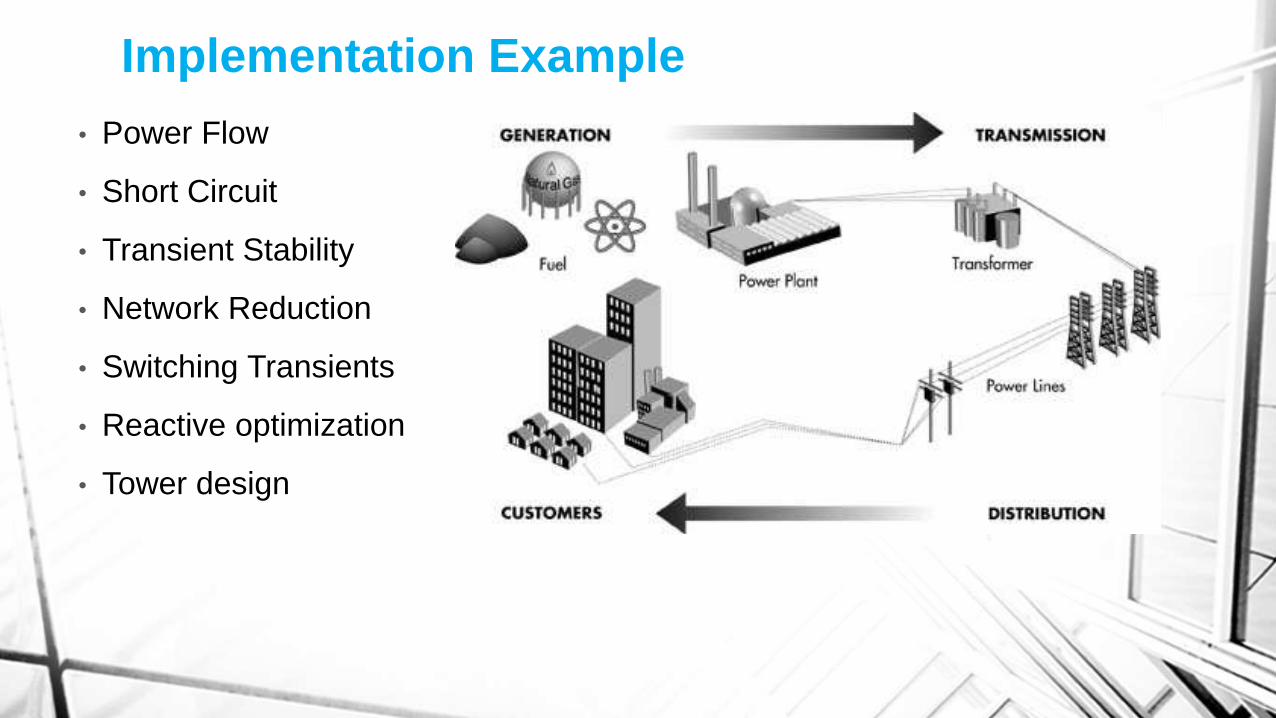
Implementation Example
• Power Flow
• Short Circuit
• Transient Stability
• Network Reduction
• Switching Transients
• Reactive optimization
• Tower design

Triangular Decomposition
• Similar to those associated with the names of Gauss,
Doolittle, Choleski, Banachiewicz, and others
• Computational variations of the basic process of
triangularizing a matrix by equivalence
transformations.
• The scheme is applicable to any nonsingular matrix,
real or complex, sparse or full, symmetric or non-
symetric.

Triangular Decomposition
• Ax = b [A][X] = [B]
• A is a nonsingular matrix, x is a column vector of unknowns, and b is a
known vector with at least one non-zero element.
• GOAL :
𝑎11 𝑎12 ⋯ 𝑎1𝑛 𝑏1𝑎21 𝑎22 ⋯ 𝑎2𝑛 𝑏2⋮ ⋮ ⋯ ⋮ ⋮
𝑎𝑛1 𝑎𝑛2 ⋯ 𝑎𝑛𝑛 𝑏𝑛
1 𝑎12(1)
⋯ 𝑎1𝑛(1)
𝑏1(1)
1 ⋯ 𝑎2𝑛(2)
𝑏2(2)
⋯ ⋮ ⋮
1 𝑏𝑛(𝑛)
Order of the derived
system

Triangular Decomposition
• 1st step
𝑎11 𝑎12 ⋯ 𝑎1𝑛 𝑏1𝑎21 𝑎22 ⋯ 𝑎2𝑛 𝑏2⋮ ⋮ ⋯ ⋮ ⋮
𝑎𝑛1 𝑎𝑛2 ⋯ 𝑎𝑛𝑛 𝑏𝑛
• 2nd step
1 𝑎12(1)
⋯ 𝑎1𝑛(1)
𝑏1(1)
𝑎21 𝑎22 ⋯ 𝑎2𝑛 𝑏2⋮ ⋮ ⋯ ⋮ ⋮
𝑎𝑛1 𝑎𝑛2 ⋯ 𝑎𝑛𝑛 𝑏𝑛
Make this equal to 1
• 𝑎1𝑗(1)
=1
𝑎11𝑎1𝑗
• 𝑏1(1)
=1
𝑎11𝑏1
1𝑎12𝑎11
⋯𝑎1𝑛𝑎11
𝑏1𝑎11
𝑎21 𝑎22 ⋯ 𝑎2𝑛 𝑏2⋮ ⋮ ⋯ ⋮ ⋮
𝑎𝑛1 𝑎𝑛2 ⋯ 𝑎𝑛𝑛 𝑏𝑛
𝑎12(1)
2nd make this equal to 11st make equal this to 0
𝑎2𝑗(1)
= 𝑎2𝑗 − 𝑎21𝑎1𝑗1
𝑏2(1)
= 𝑏2 − 𝑎21𝑏11
𝑎2𝑗(2)
=1
𝑎22(1)
𝑎2𝑗(1)
𝑏2(2)
=1
𝑎22(1)
𝑏2(1)
1st
2nd
𝑗 = 2, 𝑛
𝑗 = 3, 𝑛
Triangular Decomposition
• 2nd step (cont’d)
1 𝑎12(1)
⋯ 𝑎1𝑛(1)
𝑏1(1)
0 𝑎22(1)
⋯ 𝑎2𝑛(1)
𝑏2(1)
⋮ ⋮ ⋯ ⋮ ⋮
𝑎𝑛1 𝑎𝑛2 ⋯ 𝑎𝑛𝑛 𝑏𝑛
• 3rd step
1 𝑎121
𝑎131
⋯ 𝑎1𝑛1
𝑏11
0 1 𝑎222
⋯ 𝑎2𝑛2
𝑏22
⋮ ⋮ ⋮ ⋯ ⋮ ⋮
𝑎𝑛1 𝑎𝑛2 𝑎𝑛3 ⋯ 𝑎𝑛𝑛 𝑏𝑛
Result from 1st operation Result from 2nd operation
1 𝑎121
𝑎131
⋯ 𝑎1𝑛1
𝑏11
0 1 𝑎232
⋯ 𝑎2𝑛2
𝑏22
𝑎31 𝑎32 𝑎33 ⋯ 𝑎3𝑛 𝑏3⋮ ⋮ ⋮ ⋯ ⋮ ⋮
𝑎𝑛1 𝑎𝑛2 𝑎𝑛3 ⋯ 𝑎𝑛𝑛 𝑏𝑛
1st make this to 0 2nd make this to 0 3rd make this to 1 𝑎3𝑗(1)
= 𝑎3𝑗 − 𝑎31𝑎1𝑗1
𝑏3(1)
= 𝑏3 − 𝑎31𝑏11
𝑎3𝑗(2)
= 𝑎3𝑗(1)
− 𝑎32(1)𝑎2𝑗
2
𝑏3(2)
= 𝑏3(1)
− 𝑎32(1)𝑏2
2
𝑎3𝑗(3)
=1
𝑎33(2)
𝑎3𝑗(2)
𝑏3(3)
=1
𝑎33(2)
𝑏3(2)
1st
2nd
𝑗 = 2, 𝑛
𝑗 = 3, 𝑛
3rd𝑗 = 4, 𝑛

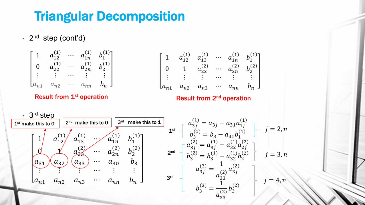
Triangular Decomposition
• 3rd step (cont’d)
• nth step
Result from 1st operation Result from 2nd operation
1 𝑎121
𝑎131
⋯ 𝑎1𝑛1
𝑏11
0 1 𝑎232
⋯ 𝑎2𝑛2
𝑏22
0 𝑎321
𝑎331
⋯ 𝑎3𝑛1
𝑏31
⋮ ⋮ ⋮ ⋯ ⋮ ⋮
𝑎𝑛1 𝑎𝑛2 𝑎𝑛3 ⋯ 𝑎𝑛𝑛 𝑏𝑛
1 𝑎121
𝑎131
⋯ 𝑎1𝑛1
𝑏11
0 1 𝑎232
⋯ 𝑎2𝑛2
𝑏22
0 0 𝑎332
⋯ 𝑎3𝑛2
𝑏32
⋮ ⋮ ⋮ ⋯ ⋮ ⋮
𝑎𝑛1 𝑎𝑛2 𝑎𝑛3 ⋯ 𝑎𝑛𝑛 𝑏𝑛
1 𝑎121
𝑎131
⋯ 𝑎1𝑛1
𝑏11
0 1 𝑎232
⋯ 𝑎2𝑛2
𝑏22
0 0 1 ⋯ 𝑎3𝑛3
𝑏31
⋮ ⋮ ⋮ ⋯ ⋮ ⋮
𝑎𝑛1 𝑎𝑛2 𝑎𝑛3 ⋯ 𝑎𝑛𝑛 𝑏𝑛Result from 3rd operation
1 𝑎121
𝑎131
⋯ 𝑎1𝑛1
𝑏11
1 𝑎232
⋯ 𝑎2𝑛2
𝑏22
1 ⋯ 𝑎3𝑛3
𝑏33
⋮ ⋮ ⋮ ⋯ ⋮ ⋮⋯ 1 𝑏𝑛
𝑛
At the end of k-th step, work on rows 1 to k has been completed
and rows k + 1 to n haven’t yet entered the process

Triangular Decomposition
• After all process has been done (nth step) the solution can be obtained by back
substitution :
𝑥𝑛 = 𝑏𝑛(𝑛)
𝑥𝑖 = 𝑏𝑖(𝑖)
− 𝑗=𝑖+1𝑛 𝑎𝑖𝑗
𝑖𝑥𝑗
𝑥𝑛−1 = 𝑏𝑛−1(𝑛−1)
− 𝑎𝑛−1,𝑛𝑛−1
𝑥𝑛
• Triangularization in the same order by column instead of rows would have produced
identically the same result.
• When A is full and n large, it can be shown that the number of multiplication-addition
operations for triangular decomposition is approximately 1
3𝑛3 compared with 𝑛3 for
inversion

Recording the Operations
• The rules for recording the forward operations of triangularization are:
1) When term 1
𝑎𝑖𝑖𝑖−1 is computed, store it in location 𝑖𝑖
2) Leave every derived term 𝑎𝑖𝑗(𝑗−1)
, 𝑖 > 𝑗 ,in the lower triangle
• The final result of triangularizing A and recording the forward operations is symbolized
as (also called the table of factors) :
𝑑11 𝑢12 𝑢12 𝑢1𝑛𝑙21 𝑑22 𝑢23 𝑢2𝑛𝑙31 𝑙32 𝑑33 𝑢3𝑛
𝑙𝑛1 𝑙𝑛2 𝑙𝑛3 𝑑𝑛𝑛
𝒅𝒊𝒊 =𝟏
𝒂𝒊𝒊(𝒊−𝟏)
𝒖𝒊𝒋 = 𝒂𝒊𝒋(𝒊)
𝒊 < 𝒋
𝒍𝒊𝒋 = 𝒂𝒊𝒋(𝒋−𝟏)
𝒊 > 𝒋
u = upper , l = lower, d = diagonal

Example – Triangularization & Recording
𝐴 =2 1 32 3 43 4 7
, find the table of factors for A..???
Ans:
1st step :
2 1 32 3 43 4 7
𝑎1𝑗(1)
=1
𝑎11𝑎1𝑗
1st make this to 1 𝑎11(1)
=1
22 = 1
𝑎12(1)
=1
21 =
1
2
𝑎13(1)
=1
23 =
3
2
Table of factors
1 1 2 3 22 3 43 4 7
Result :
Record this as 𝑑11
Record this as
𝑢12& 𝑢13
1 2 1 2 3 2? ? ?? ? ?
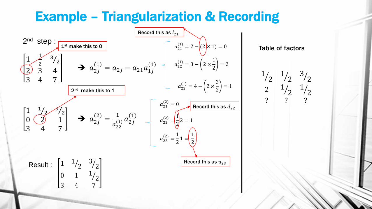
Example – Triangularization & Recording
2nd step :
11
2 3 2
2 3 43 4 7
𝑎2𝑗(1)
= 𝑎2𝑗 − 𝑎21𝑎1𝑗(1)
1 1 2 3 2
0 2 13 4 7
𝑎2𝑗(2)
=1
𝑎22(1) 𝑎2𝑗
(1)
1st make this to 0 𝑎21(1)
= 2 − (2 × 1) = 0
𝑎22(1)
= 3 − 2 ×1
2= 2
𝑎23(1)
= 4 − 2 ×3
2= 1
Table of factors
2nd make this to 1
𝑎21(2)
= 0
𝑎22(2)
=1
22 = 1
𝑎23(2)
=1
21 =
1
2
1 1 2 3 2
0 1 1 23 4 7
Result :
Record this as 𝑙21
Record this as 𝑑22
Record this as 𝑢23
1 2 1 2 3 2
2 1 2 1 2? ? ?

Example – Triangularization & Recording
3rd step :
1 1 2 3 2
0 11
2
3 4 7
𝑎3𝑗(1)
= 𝑎3𝑗 − 𝑎31𝑎1𝑗(1)
1 1 2 3 2
0 11
2
05
2
5
2
𝑎3𝑗(2)
= 𝑎3𝑗(1)
− 𝑎32(1)𝑎2𝑗(2)
1st make this to 0 𝑎31(1)
= 3 − (3 × 1) = 0
𝑎32(1)
= 4 − 3 ×1
2=5
2
𝑎33(1)
= 7 − 3 ×3
2=5
2
Table of factors
1 2 1 2 3 2
2 1 2 1 2
3 5 2 ?2nd make this to 0
𝑎31(2)
= 0
𝑎32(2)
=5
2−5
21 = 0
𝑎33(2)
=5
2−5
2
1
2=
5
4
Record this as 𝑙31
Record this as 𝑙32
Cont’d….

Example – Triangularization & Recording
3rd step (cont’d):
1 1 2 3 2
0 1 1 2
0 0 5 4
𝑎3𝑗(3)
=1
𝑎33(2) 𝑎3𝑗
(2)
3rd make this to 1 Table of factors
1 2 1 2 3 2
2 1 2 1 2
3 5 2 4 5
𝑎31(3)
= 0
𝑎32(3)
= 0
𝑎33(3)
=1
5 4
5
4= 1
Record this as 𝑑33

Computing Direct Solutions
• It is convenient in symbolizing the operations for obtaining direction solutions to define
some special matrices in term of the element of the table of factors:
𝐷𝑖 ∶ 𝑅𝑜𝑤 𝑖 = 0,0, . . , 0, 𝑑𝑖𝑖 , 0, … 0,0
𝐿𝑖 ∶ 𝐶𝑜𝑙 𝑖 = 0,0, . . , 0,1, −𝑙𝑖+1,𝑖 , −𝑙𝑖+2,𝑖 , …−𝑙𝑛−1,𝑖,, −𝑙𝑛,𝑖𝑡
𝐿𝑖∗ ∶ 𝐶𝑜𝑙 𝑖 = −𝑙𝑖,1, −𝑙𝑖,2, … , −𝑙𝑖,𝑖−1, 1,0, … 0,0
𝑈𝑖 ∶ 𝑅𝑜𝑤 𝑖 = 0,0,… 0,1, −𝑢𝑖,𝑖+1, −𝑢𝑖,𝑖+2, …−𝑢𝑖,𝑛−1, −𝑢𝑖,𝑛
𝑈𝑖∗ ∶ 𝐶𝑜𝑙 𝑖 = −𝑢1,𝑖 , −𝑢2,𝑖 , …−𝑢𝑖−1,𝑖 , 1,0, … 0,0
𝑡
• The invese of this matrix are trivial. Inverse of matrix 𝐷𝑖 involves only the reciprocal of
the element 𝑑𝑖𝑖, and inverse of matrices 𝐿𝑖, 𝐿𝑖∗, 𝑈𝑖, 𝑈𝑖
∗ involve only a reversal of algebraic
signs of the off-diagonal elements
D,L,U are nonsingular matrices which
differ from the unit matrix only in the
row or column indicated

Computing Direct Solutions
• The forward and backward substitution operations on the column vector b that transform
it to x can be expressed as premultiplications by matrices 𝐷𝑖 , 𝐿𝑖 or 𝐿𝑖∗, and 𝑈𝑖 or 𝑈𝑖
∗.
• Solution of 𝐴𝑥 = 𝑏 can be expressed as indicated :
a) 𝑈1𝑈2…𝑈𝑛−2𝑈𝑛−1𝐷𝑛𝐿𝑛−1𝐷𝑛−1𝐿𝑛−2…𝐿2𝐷2𝐿1𝐷1𝑏 = 𝐴−1𝑏 = 𝑥
b) 𝑈1𝑈2…𝑈𝑛−2𝑈𝑛−1𝐷𝑛𝐿𝑛∗ 𝐷𝑛−1𝐿𝑛−1
∗ …𝐿3∗𝐷2𝐿2
∗𝐷1𝑏 = 𝐴−1𝑏 = 𝑥
c) 𝑈2∗𝑈3
∗…𝑈𝑛−1∗ 𝑈𝑛
∗𝐷𝑛𝐿𝑛−1𝐷𝑛−1𝐿𝑛−2…𝐿2𝐷2𝐿1𝐷1𝑏 = 𝐴−1𝑏 = 𝑥
d) 𝑈2∗𝑈3
∗…𝑈𝑛−1∗ 𝑈𝑛
∗𝐷𝑛𝐿𝑛∗ 𝐷𝑛−1𝐿𝑛−1
∗ …𝐿3∗𝐷2𝐿2
∗𝐷1𝑏 = 𝐴−1𝑏 = 𝑥
• (a) describes the forward and backward substitution operations that would be performed
on b if it augmented A during triangularization by column, while (b) describes the same
result for triangularization by rows
• (c) and (d) describes other sequences of the same operations giving the same result
Depending on programming
techniques, one of these will prove to
be the most convenient

Computing Direct Solutions
• Example :
𝐴 =2 1 32 3 43 4 7
, table factors for A (from previous slide) =
• With b given b =6914
, solve x if 𝐴−1𝑏 = 𝑥
• Using direct solution formula from previous slide, from equation (a)
1 −1
2−
1
2
11
1
1 −1
2
1
11
4
5
11
−5
21
11
2
1
1−2 1−3 1
1
2
11
6914
=111
1 2 1 2 3 2
2 1 2 1 2
3 5 2 4 5
𝑼𝟏 𝑼𝟐 𝑳𝟐𝑫𝟑 𝑳𝟏𝑫𝟐 𝒃𝑫𝟏 𝒙

Computing Direct Solutions
• Given 𝑥, the vector 𝑏 can be obtained as:
a) 𝐷1−1𝐿1
−1𝐷2−1𝐿2
−1…𝐿𝑛−1−1 𝐷𝑛
−1𝑈𝑛−1−1 𝑈𝑛−2
−1 …𝑈2−1𝑈1
−1𝑥 = 𝐴𝑥 = 𝑏
b) 𝐷1−1(𝐿2
∗ )−1𝐷2−1(𝐿3
∗ )−1…(𝐿𝑛∗ )−1𝐷𝑛
−1𝑈𝑛−1−1 𝑈𝑛−2
−1 …𝑈2−1𝑈1
−1𝑥 = 𝐴𝑥 = 𝑏
• With x given x =111
, solve b if 𝐴𝑥 = 𝑏
Example: (Matrix A is same as previous example)
21
1
12 13 1
12
1
115
21
11
5
4
1
11
2
1
1 1
2
3
2
11
111
=
6914
𝑫𝟏−𝟏 𝑳𝟏
−𝟏 𝑳𝟐−𝟏𝑫𝟐
−𝟏 𝑼𝟐−𝟏𝑫𝟑
−𝟏𝒃𝑼𝟏
−𝟏 𝒙
1 2 1 2 3 2
2 1 2 1 2
3 5 2 4 5
Table of factors for A

Computing Direct Solutions
• Given 𝐴𝑡𝑦 = 𝑐, the vector 𝑐 can be obtained as:
a) 𝐷1𝐿1𝑡𝐷2𝐿2
𝑡 …𝐿𝑛−1𝑡 𝐷𝑛𝑈𝑛−1
𝑡 𝑈𝑛−2𝑡 …𝑈2
𝑡𝑈1𝑡𝑐 = (𝐴𝑡)−1𝑐 = 𝑦
b) (𝑈1𝑡)−1(𝑈2
𝑡)−1… 𝑈𝑛−2𝑡 −1 𝑈𝑛−1
𝑡 −1𝐷𝑛−1 𝐿𝑛−1
𝑡 −1…(𝐿2𝑡 )−1𝐷2
−1(𝐿1𝑡 )−1𝐷1
−1𝑦 = 𝐴𝑡𝑦 = 𝑐
• With c given c =9917
, solve y if 𝐴𝑡𝑦 = 𝑐
Example: (Matrix A is same as previous example)
1
2
11
1 −2 −31
1
11
2
1
1
1 −5
2
1
11
4
5
11
−1
21
11
21
3
21
9917
=
211
1 2 1 2 3 2
2 1 2 1 2
3 5 2 4 5
Table of factors for A
𝑫𝟏 𝑳𝟏𝒕 𝑫𝟐 𝑫𝟑 𝒄 𝒚𝑳𝟐
𝒕 𝑼𝟐𝒕 𝑼𝟏
𝒕
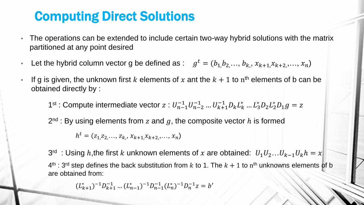
Computing Direct Solutions
• The operations can be extended to include certain two-way hybrid solutions with the matrix
partitioned at any point desired
• Let the hybrid column vector g be defined as : 𝑔𝑡 = (𝑏1,𝑏2,…, 𝑏𝑘,, 𝑥𝑘+1,𝑥𝑘+2,,…, 𝑥𝑛)
• If g is given, the unknown first 𝑘 elements of 𝑥 ant the 𝑘 + 1 to nth elements of b can be
obtained directly by :
1st : Compute intermediate vector 𝑧 : 𝑈𝑛−1−1 𝑈𝑛−2
−1 …𝑈𝑘+1−1 𝐷𝑘𝐿𝑘
∗ …𝐿3∗𝐷2𝐿2
∗𝐷1𝑔 = 𝑧
2nd : By using elements from 𝑧 and 𝑔, the composite vector ℎ is formed
3rd : Using ℎ,the first 𝑘 unknown elements of 𝑥 are obtained: 𝑈1𝑈2…𝑈𝑘−1𝑈𝑘ℎ = 𝑥
4th : 3rd step defines the back substitution from 𝑘 to 1. The 𝑘 + 1 to nth unknowns elements of b
are obtained from:
(𝐿𝑘+1∗ )−1𝐷𝑘+1
−1 …(𝐿𝑛−1∗ )−1𝐷𝑛−1
−1 (𝐿𝑛∗ )−1𝐷𝑛
−1𝑧 = 𝑏′
ℎ𝑡 = (𝑧1,𝑧2,…, 𝑧𝑘,, 𝑥𝑘+1,𝑥𝑘+2,,…, 𝑥𝑛)

Computing Direct Solutions
• Example, given the hybrid vector 𝑔 such that 𝑔𝑡 = (𝑏1,𝑥2,𝑥3) = 6,1,1
1st : The intermediate vector 𝑧
3rd : Compute 𝑥
1
11
21
1
21
1
611
=
33
21
𝑫𝟏𝑼𝟐−𝟏 𝒈 𝒛
2nd : Vector ℎ = 𝑧1,𝑥2,𝑥3 = (3,1,1)
1 −1
2−3
21
1
311
=111
𝑼𝟏𝒉 𝒙
4th : Compute elements 𝑏2 and 𝑏3
12 1
1
12
1
11
35
21
11
5
4
33
21
=3914
𝑫𝟐−𝟏(𝑳𝟐
∗ )−𝟏 𝒛 𝒃′(𝑳𝟑∗ )−𝟏 𝑫𝟑
−𝟏
Sparsity and Optimal Ordering
• When the matrix triangularized is sparse, the order in which rows are
processed affects the number of nonzero terms in the resultant upper
triangle
• If a programming scheme is used which process and stores only nonzero
terms, a very great saving in operations and memory can be achieved
• An efficient algorithm for determining the absolute optimal order hasn’t
been developed, and it appears to be a practical impossibility
• Scheme for near-optimal ordering introduced

Iterative vs. direct methods
• Direct solutions method producing exact solution in finite number of steps (in exact arithmetic)
• Iterative methods begin with initial guess for solution and successively improve it until desired accuracy attained
• In theory, it might take infinite number of iterations to converge to exact solution, but in practice iterations are terminated when residual is as small as desired
• For some types of problems, iterative methods have significant advantages over direct methods

Comparative advantages for a Sparse Matrix
1. The table of factors can be obtained in a small fraction of the time required for the inverse
2. The storage requirement is small, permitting much larger system to be solved
3. Direct solutions can be obtained much faster unless the independent vector is extremely sparse
4. Round-off error is reduced
5. Modifications due to changes in the matrix can be made much faster