directional pricing theory in electricity 32th usaee/iaee north american conference hotel captain...

Directional Pricing Theory in Electricity

32th USAEE/IAEE North American Conference

Hotel Captain Cook, Anchorage, AK

July 29, 2013

Akira Maeda (University of Tokyo)

Makiko Nagaya (Showa Women’s University)

This research was supported in part by the Environment Research and Technology Development Fund (S10-1(3)) of the Ministry of the Environment, Japan.

Motivation

• Standard economic theory presumes that prices are non-directional:– Consider a transaction of Good X between two agents.

– Assuming there is no transaction cost (inc. carrying cost, etc.), prices, b and s must be the same. Otherwise, there will be an arbitrage opportunity.

• However, there may exist exceptions in the real world.– Electricity: non-storable; runs in one direction through

transmission line.

2

Agent BAgent A

Good X(buying price: b)

Good X(selling price: s)

Feed-in-tariff (FIT) and smart grids

• Due to recent developments in electricity production and transmission technologies, the distinction b/w generators and consumers is becoming unclear.– Consumer can not only buy electricity from the utility, but also

sell electricity to the utility.– Examples include the “smart grid” concept.

• Pricing in electricity is becoming more political rather than economical.– Some countries introduce the FIT policy to promote “high-cost”

renewable energy generators such as photovoltaics (PVs), wind powers, etc. –Germany, Spain, Japan (from July, 2012)

– Consumers can sell it at a higher price.

3

Purpose

• to develop a theory for pricing policy that allows the market operators (or market regulators) to set directional prices,

• showing how pricing practices would be complicated in advanced electricity systems such as smart grids.

– a model of directional pricing scheme

– its mathematics

– its feature

– some implications

Note: Earlier versions have been presented some conferences including IAEE European Conference in Venice last year.

4

The model

• Consider an electricity customer who has his own generator and is connected to an electric utility firm through a single transmission line. Using the generator, the customer can sell the electricity to the

utility firm at a price different from his buying price.

5

Customer-ownedgenerator

Electric utility firmCustomer

x

y(buying price: b)

z(selling price: s)

Contrast to a two-line setting

• If electricity transmission lines are physically separated for buying and selling, the customer is able to make simultaneous trades of buying and selling.

6



x

y(buying price: b)

z(selling price: s)

Contrast to a two-line setting, cont’d

• If b < s, the customer can enjoy an arbitrage.• To avoid such an arbitrage opportunity, the price setting

is restricted such that b s holds.

7



x

y(buying price: b)

z(selling price: s)

q

If b < s,q (s-b) as q


• The basic idea of the FIT policy is to promote renewable energy sources that have relatively higher unit costs.

• Thus, b < s is the most probable scheme to set.

• This fact indicates that the two-line model does not work for the price setting under the FIT policies.

8

Contrast to a separate generator setting

• If customer-owned generators are separated, production and consumption are separated as well.

• This makes the model reduce to a model of standard electric systems.

• Thus, it cannot help identify a feature of the FIT policies either that of smart grids.

9



x

y(buying price: b)

z (= x)(selling price: s)

The feature of the single-line setting

• Under the single line setting, such arbitrage opportunities are excluded because flows are always directional. That is, either

y 0 and z = 0, or

y = 0 and z 0

can occur, which removes the restriction on the price setting.

10



x

y(buying price: b)

z(selling price: s)

Pricing scheme

• Directional pricing scheme– A customer cannot simultaneously purchase and sell the good.– When a customer purchases the good, the buying price is

applied to the trade.– On the other hand, when a customer sells the good, the selling

price is applied to the trade.

• The customer’s behavior under the scheme:utility max-problem with– budget constraint,– physical constraint of electricity flow.

11

Mixed-integer programming (MIP)

12

either y = 0 or z = 0



x

y(buying price: b)

z(selling price: s)


13




x

y(buying price: b)

z(selling price: s)

The two separate line setting allows the customer to make buying and selling simultaneously.Arbitrage opportunities exit.

Contrast to a separate generator setting

14




x

y(buying price: b)

z (= x)(selling price: s)

x = z

The model reduces to:

,max ,

. .

y zU y w

s t

C z w b y m s z

Mixed-integer programming (MIP)

15




x

y(buying price: b)

z(selling price: s)

Assumptions

Assumption 1: “Electricity is a small part of consumption.”The welfare function is quasi-linear, i.e.,

Also, u(X) satisfies the Inada condition, i.e.,

Assumption 2: “No economy of scale; no sunk cost.”There is no fixed cost, i.e.,

Marginal cost is monotonously increasing from the origin, i.e.,

16

,U X W u X W

0

limX

u X

lim 0X

u X

0 0C

0 0MC

FONCs for the solution

Due to the mixed-integer programming nature, the set of complementary slackness conditions plays a key role:

17

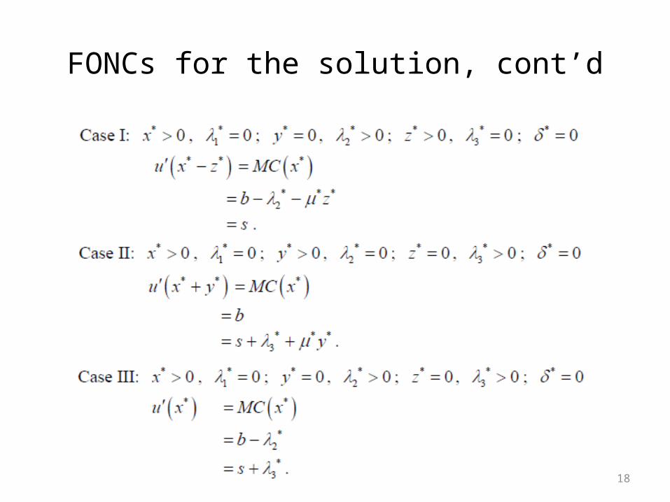
FONCs for the solution, cont’d

18

Getting analytical solution

Following additional assumptions are enough for us to have an analytical solution:

Assumption 3:u(X) has the form of power function:

Assumption 4:C(X) has the form of quadratic function:

19

1 1

1

Xu X A

21

2C X cX

Solution on the b-s plane

20

“Sell” region

“Buy” regionU

* in

crea

ses

U* increases

“No buy, no sell” region

b

s

0

*

1

AU f s m

*

1

AU f b m

f s f bThe curve of

1

1c A c

1

1c A c

* min1

AU f X m

1 1

1 21

1 2f X A X X

c

Solution on the b-s plane, cont’d

21

Only selling to the utility firm can occur and its inverse supply curve is given by:

“Sell” region

“Buy” region

U*

incr

ease

s

U* increases


b

s

0

*

1

AU f s m

*

1

AU f b m

f s f bThe curve of

1

1c A c

1

1c A c

* min1

AU f X m

1 1

121

1 2f X A X X

c


22

In this region, there exists a boundary between “sell” and “buy”.The choice is determined by the comparison of possible welfare gains:Demand curve:

Supply curve:

“Sell” region

“Buy” region

U*

incr

ease

s

U* increases


b

s

0

*

1

AU f s m

*

1

AU f b m

f s f bThe curve of

1

1c A c

1

1c A c

* min1

AU f X m

1 1

121

1 2f X A X X

c


23

Only buying from the utility firm can occur and its inverse demand curve is given by:

“Sell” region

“Buy” region

U*

incr

ease

s

U* increases


b

s

0

*

1

AU f s m

*

1

AU f b m

f s f bThe curve of

1

1c A c

1

1c A c

* min1

AU f X m

1 1

121

1 2f X A X X

c


24

There is neither selling nor buying: the customer chooses to use electricity produced by his generator in the form of “stand-alone.”

“Sell” region

“Buy” region

U*

incr

ease

s

U* increases


b

s

0

*

1

AU f s m

*

1

AU f b m

f s f bThe curve of

1

1c A c

1

1c A c

* min1

AU f X m

1 1

121

1 2f X A X X

c


25




x

y(buying price: b)

z(selling price: s)

The two separate line setting allows the customer to make buying and selling simultaneously.


• No-arbitrage restriction for the customer excludes the possibility of b < s.

• It results in the existence of an infeasible region.

26

“Sell” region

“Buy” region


b

s

0

s b

1

1c A c

1

1c A c Infe

asibl

e re

gion

Net demand / supply functions

27X

b X

1

1f c A c

1

1c A c

f X

X

s X

1

1f c A c

1

1c A c

f X

Net demand / supply curves

• The existence of solutions for the case of b < s makes the directional pricing scheme very distinctive.

28

Y(b,s)

*b s

1

1c A c

s

b

0

1 1

A s s c

Z(b,s)

*s b

1

1c A c

b

s

0

1 1

b c A b

Net demand curve as a function of buying price b for the case of

Net supply curve as a function of selling price s for the case of

1

1 1b c A s

1

1 1b c A s

Conclusions

• A consumer’s model for directional pricing schemes is developed. A typical application is strategic pricing in advanced electricity systems.

• The analytical solution of the model depicts a complicated feature of directional pricing schemes.– Net demand and supply curves can be discontinuous.

– The rate design has a much higher degree of freedom than that of traditional electric utility pricing.

– Typical market transaction and/or consumer behavior models studied so far in economic theory do not work for the analysis of the FIT policies.

– Our result contributes to a better understanding of the rate design for the FIT policy formulation as well as for advances in smart grids.

29

directional pricing theory in electricity 32th usaee/iaee north american conference hotel captain...

Documents

electricity customer

electricity production

price setting

directional pricing

contdif b s

b s holds

pricing policy

single line setting