dirichlet mixtures - computational biology - university of california
TRANSCRIPT

Dirichlet Mixtures: A Method for Improved Detection of Weakbut Signi�cant Protein Sequence Homology
Kimmen Sj�olandery
Computer Science
U.C. Santa Cruz
Kevin KarplusComputer Engineering
U.C. Santa Cruz
Michael BrownComputer Science
U.C. Santa Cruz
Richard HugheyComputer Engineering
U.C. Santa Cruz
Anders KroghThe Sanger Centre
England
I. Saira MianLawrence Berkeley Laboratory
U.C. Berkeley
David HausslerComputer Science
U.C. Santa Cruz
Abstract
We present a method for condensing the information in multiple alignments of proteins into a mixtureof Dirichlet densities over amino acid distributions. Dirichlet mixture densities are designed to becombined with observed amino acid frequencies to form estimates of expected amino acid probabilitiesat each position in a pro�le, hidden Markov model, or other statistical model. These estimates givea statistical model greater generalization capacity, so that remotely related family members can bemore reliably recognized by the model. This paper corrects the previously published formula forestimating these expected probabilities, and contains complete derivations of the Dirichlet mixtureformulas, methods for optimizing the mixtures to match particular databases, and suggestions fore�cient implementation.
Keywords: Substitution matrices, pseudocount methods, Dirichlet mixture priors, pro�les,hidden Markov models.
yTo whom correspondence should be addressed. Mailing address: Baskin Center for Computer Engineering andInformation Sciences, Applied Sciences Building, University of California at Santa Cruz, Santa Cruz, CA 95064.Phone: (408) 459-3430, Fax: (408) 459-4829. Mail to Karplus, Brown, Hughey and Haussler may be sent to the BaskinCenter for Computer Engineering and Information Sciences, Applied Sciences Building, University of California atSanta Cruz, Santa Cruz, CA 95064. Mail to Krogh should be sent to The Sanger Centre, Hinxton Hall, Hinxton,Cambs CB10 1RQ, England. Mail to Mian should be sent to Life Sciences Division (Mail Stop 29-100), LawrenceBerkeley Laboratory, University of California, Berkeley, CA 94720.

1 Introduction
One of the main techniques used in protein sequence analysis is the identi�cation of homologous proteins|proteins which share a common evolutionary history and almost invariably have similar overall structureand function (Doolittle, 1986). Homology is straightforward to infer when two sequences share 25% residueidentity over a stretch of 80 or more residues (Sander and Schneider, 1991). Recognizing remote homologs,with lower primary sequence identity, is more di�cult. Finding these remote homologs is one of the primarymotivating forces behind the development of statistical models for protein families and domains, such aspro�les and their many o�shoots (Gribskov et al., 1987; Gribskov et al., 1990; Bucher et al., 1996; Barton andSternberg, 1990; Altschul et al., 1990; Waterman and Perlwitz, 1986; Thompson et al., 1994a; Thompson etal., 1994b; Barton and Sternberg, 1990; Bowie et al., 1991; L�uthy et al., 1991; Bucher et al., 1996), Position-Speci�c Scoring Matrices (Heniko� et al., 1990), and hidden Markov models (HMMs) (Churchill, 1989;White et al., 1994; Stultz et al., 1993; Krogh et al., 1994; Hughey and Krogh, 1996; Baldi et al., 1992;Baldi and Chauvin, 1994; Asai et al., 1993; Eddy, 1995; Eddy et al., 1995; Eddy, 1996).
We address this problem by incorporating prior informationabout amino acid distributions that typicallyoccur in columns of multiple alignments into the process of building a statistical model. We present amethod to condense the information in databases of multiple alignments into a mixture of Dirichlet densities(Bernardo and Smith, 1994; Berger, 1985; Santner and Du�y, 1989) over amino acid distributions, and tocombine this prior informationwith the observed amino acids to formmore e�ective estimates of the expecteddistributions. Multiple alignments used in these experiments were taken from the Blocks database (Heniko�and Heniko�, 1991). We use Maximum Likelihood (Duda and Hart, 1973; Nowlan, 1990; Dempster et al.,1977) to estimate these mixtures|that is, we seek to �nd a mixture that maximizes the probability of theobserved data. Often, these densities capture some prototypical distributions. Taken as an ensemble, theyexplain the observed distributions in columns of multiple alignments.
With accurate prior information about which kinds of amino acid distributions are reasonable in columnsof alignments, it is possible with only a few sequences to identify which prototypical distribution may havegenerated the amino acids observed in a particular column. Using this informed guess, we adjust theexpected amino acid probabilities to include the possibility of amino acids that may not have been seen butare consistent with observed amino acid distributions. The statistical models produced are more e�ectiveat generalizing to previously unseen data, and are often superior at database search and discriminationexperiments (Wang et al., 1996; Hughey and Krogh, 1996; Karplus, 1995a; Bailey and Elkan, 1995; Tatusovet al., 1994; Heniko� and Heniko�, 1996; Brown et al., 1993).
1.1 Database search using statistical models
Statistical models for proteins capture the statistics de�ning a protein family or domain. These modelshave two essential aspects: 1) parameters for every position in the molecule or domain that express theprobabilities of the amino acids, gap initiation and extension, and so on, and 2) a scoring function forsequences with respect to the model.
Statistical models do not use percentage residue identity to determine homology. Instead, these modelsassign a probability score1 to sequences, and then compare the score to a cuto�. Most models (includingHMMs and pro�les) make the simplifying assumption that each position in the protein is generated inde-pendently. Under this assumption, the score for a sequence aligning to a model is equal to the productof the probabilities of aligning each residue in the protein to the corresponding position in the model. Inhomolog identi�cation by percentage residue identity, if a protein aligns a previously unseen residue at aposition it is not penalized; it loses that position, but can still be recognized as homologous if it matches at asu�cient number of other positions in the search protein. However, in statistical models, if a protein alignsa zero-probability residue at a position, the probability of the sequence with respect to the model is zero,regardless of how well it may match the rest of the model. Because of this, most statistical models rigorouslyavoid assigning residues probability zero, and accurate estimates for the amino acids at each position areparticularly important.
1Some methods report a cost rather than a probability score; these are closely related (Altschul, 1991).
2

1.2 Using prior information about amino acid distributions
The parameters of a statistical model for a protein family or domain are derived directly from sequences inthe family or containing the domain. When we have few sequences, or a skewed sample,2 the raw frequenciesare a poor estimate of the distributions which we expect to characterize the homologs in the database.Models that use these raw frequencies may recognize the sequences used to train the model, but will notgeneralize well to recognizing remoter homologs.
It is illuminating to consider the analogous problem of assessing the fairness of a coin. A coin is said tobe fair if Prob(heads) = Prob(tails) = 1=2. If we toss a coin three times, and it comes up heads each time,what should our estimate be of the probability of heads for this coin? If we use the observed raw frequencies,we would set the probability of heads to 1. But, if we assume that most coins are fair, then we are unlikelyto change this a priori assumption based on only a few tosses. Given little data, we will believe our priorassumptions remain valid. On the other hand, if we toss the coin an additional thousand times and it comesup heads each time, few will insist that the coin is indeed fair. Given an abundance of data, we will discountany previous assumptions, and believe the data.
When we estimate the expected amino acids in each position of a statistical model for a protein family, weencounter virtually identical situations. Fix a numbering of the amino acids from 1 to 20. Then, each columnin a multiple alignment can be represented by a vector of counts of amino acids of the form ~n = (n1; : : : ; n20),where ni is the number of times amino acid i occurs in the column represented by this count vector, andj~nj =
Pi ni. The estimated probability of amino acid i is denoted p̂i. If the raw frequencies are used to set
the probabilities, then p̂i := ni= j~nj. Note that we use the symbol `:=' to denote assignment, to distinguishit from equality, since we compute p̂i di�erently in di�erent parts of the paper.
Consider the following two scenarios. In the �rst, we have only three sequences from which to estimatethe parameters of the model. In the alignment of these three sequences we have a column containing onlyisoleucine, and no other amino acids. With such a small sample, we cannot rule out the possibility thathomologous proteins may have di�erent amino acids at this position. In particular, we know that isoleucineis commonly found in buried beta strand environments, and leucine and valine often substitute for it in theseenvironments. Thus, our estimate of the expected distribution at this position would sensibly include theseamino acids, and perhaps the other amino acids as well, albeit with smaller probabilities.
In a second scenario, we have an alignment of 100 varied sequences and again �nd a column containingonly isoleucine, and no other amino acids. In this case, we have much more evidence that isoleucine is indeedconserved at this position, and thus generalizing the distribution at this position to include similar residuesis probably not a good idea. In this situation, it makes more sense to give less importance to prior beliefsabout similarities among amino acids, and more importance to the actual counts observed.
The natural solution is to introduce prior information into the construction of the statistical model.The method we propose interpolates smoothly between reliance on the prior information concerning likelyamino acid distributions, in the absence of data, and con�dence in the amino acid frequencies observed ateach position, given su�cient data.
1.3 What is a Dirichlet density?
A Dirichlet density � (Berger, 1985; Santner and Du�y, 1989) is a probability density over the set of all proba-bility vectors ~p (i.e., pi � 0 and
Pi pi = 1). Proteins have a 20-letter alphabet, with pi = Prob(amino acid i).
Each vector ~p represents a possible probability distribution over the 20 amino acids.A Dirichlet density has parameters ~� = �1; : : : ; �20, with �i > 0. The value of the density for a
particular vector ~p is
�(~p) =
Q20i=1 p
�i�1i
Z; (1)
2Skewed samples can arise in two ways. In the �rst, the sample is skewed simply from the luck of the draw. Thiskind of skew is common in small samples, and is akin to tossing a fair coin three times and observing three heads ina row. The second type of skew is more insidious, and can occur even when large samples are drawn. In this kind ofskew, one subfamily is over-represented, such that a large fraction of the sequences used to train the statistical modelare minor variants of each other. In this kind of skew, sequence weighting schemes are necessary to compensate forthe bias in the data.
3

where Z is the normalizing constant that makes � sum to unity. The mean value of pi given a Dirichletdensity with parameters ~� is
Epi = �i= j~�j ; (2)
where j~�j =P
i �i.The second moment Epi pj , for the case i 6= j is given by
Epi pj =�j�i
j~�j (j~�j+ 1): (3)
When i = j, the second moment Ep2i is given by
Ep2i =�i (�i + 1)
j~�j (j~�j+ 1): (4)
We chose Dirichlet densities because of their mathematical convenience: a Dirichlet density is a conjugateprior|i.e., the posterior of a Dirichlet density has the same form as the prior (see, for example, Section A.4).
1.4 What is a Dirichlet Mixture?
A mixture of Dirichlet densities is a collection of individual Dirichlet densities that function jointly toassign probabilities to distributions. For any distribution of amino acids, the mixture as a whole assigns aprobability to the distribution by using a weighted combination of the probabilities given the distributionby each of the components in the mixture. These weights are called mixture coe�cients. Each individualdensity in a mixture is called a component of the mixture.
A Dirichlet mixture density � with l components has the form
� = q1�1 + : : :+ ql�l ; (5)
where each �j is a Dirichlet density speci�ed by parameters ~�j = (�j;1; : : : ; �j;20) and the numbers q1; : : : ; qlare the mixture coe�cients and sum to 1.
The symbol � refers to the entire set of parameters de�ning a prior. In the case of a mixture, � =(~�1; : : : ; ~�l; q1 : : : ; ql), whereas in the case of a single density, � = (~�).
1.4.1 Interpreting the parameters of a Dirichlet mixture
Since a Dirichlet mixture describes the typical distributions of amino acids in the data used to estimate themixture, it is useful to look in some detail at each individual component of the mixture to see what distri-butions of amino acids it favors. We include in this paper a 9-component mixture estimated on the Blocksdatabase (Heniko� and Heniko�, 1991), a close variant of which has been used in experiments elsewhere(Tatusov et al., 1994; Heniko� and Heniko�, 1996).
A couple of comments about how we estimated this mixture density are in order.First, the decision to use nine components was somewhat arbitrary. As in any statistical model, a balance
must be struck between the complexity of the model and the data available to estimate the parameters ofthe model. A mixture with too few components will have a limited ability to represent di�erent contexts forthe amino acids. On the other hand, there may not be su�cient data to precisely estimate the parametersof the mixture if it has too many components. We have experimented with mixtures with anywhere fromone to thirty components; in practice, nine components appears to be the best compromise with the data wehave available. Also, a 9-component mixture uses 188 parameters, slightly fewer than the 210 of a symmetricsubstitution matrix, so that better results with the Dirichlet mixture cannot be attributed to having moreparameters to �t to the data.
Second, there are many di�erent mixtures having the same number of components that give basicallythe same results. This re ects the fact that Dirichlet mixture densities attempt to �t a complex space, andthere are many ways to �t this space. Optimization problems such as this are notoriously di�cult, and wemake no claim that this mixture is globally optimal. This mixture works quite well, however, and is betterthan many other 9-component local optima that we have found.
Table 1 gives the parameters of this mixture. Table 2 lists the preferred amino acids for each componentin the mixture, in order by the ratio of the mean probability of the amino acids in a component to thebackground probability of the amino acids. An alternative way to characterize a component is by giving
4

the mean expected amino acid probabilities and the variance around the mean. Formulas to compute thesequantities were given in Section 1.3.
The value j~�j =P20
i=1 �i is a measure of the variance of the component about the mean. Higher valuesof j~�j indicate that distributions must be close to the mean of the component in order to be given highprobability by that component. In mixtures we have estimated, components having high j~�j tend to givehigh probability to combinations of amino acids which have similar physiochemical characteristics and areknown to substitute readily for each other in particular environments. By contrast, when j~�j is small, thecomponent favors pure distributions conserved around individual amino acids. A residue may be representedprimarily by one component (as proline is) or by several components (as isoleucine and valine are).3
1.5 Comparison with other methods for computing these probabilities
In this section we compare the di�erent results obtained when estimating the expected amino acids usingthree methods: Dirichlet mixture priors, substitution matrices, and pseudocounts. A brief analysis of thedi�erences is contained in the subsections below. In addition, we give examples of the di�erent resultsproduced by these methods in several tables. Tables 4{7 show the di�erent amino acid estimates producedby each method for the cases where 1 to 10 isoleucines are aligned in a column, with no other amino acids.
1.5.1 Substitution matrices
The need for incorporating prior information about amino acid distributions into protein alignmentmotivatedthe development of amino acid substitution matrices. These have been used e�ectively in database searchand discrimination tasks (Heniko� and Heniko�, 1993; Jones et al., 1992; George et al., 1990; Heniko� andHeniko�, 1992; Altschul, 1991; Claverie, 1994; Rodionov and Johnson, 1994).
There are two drawbacks associated with the use of substitution matrices. First, each amino acidhas a �xed substitution probability with respect to every other amino acid. In any particular substitutionmatrix, to paraphrase Gertrude Stein, a phenylalanine is a phenylalanine is a phenylalanine. However, aphenylalanine seen in one context, for instance, a position requiring an aromatic residue, will have di�erentsubstitution probabilities than a phenylalanine seen in a context requiring a large non-polar residue. Second,only the relative frequency of amino acids is considered, while the actual number observed is ignored.Thus, in substitution-matrix-based methods, the expected amino acid probabilities are identical for anypure phenylalanine column, whether it contains 1, 3, or 100 phenylalanines. All three situations are treatedidentically, and the estimates produced are indistinguishable.
1.5.2 Pseudocount methods
Pseudocount methods can be viewed as a special case of Dirichlet mixtures, where the mixture consists ofa single component. In these methods, a �xed value is added to each observed amino acid count, and thenthe counts are normalized. More precisely, the formula used is p̂i := (ni + zi)=(
Pj nj + zj), where each
zj is some constant. Pseudocount methods have many of the desirable properties of Dirichlet mixtures|inparticular, that the estimated amino acids converge to the observed frequencies as the number of observationsincreases|but because they have only a single component, they are unable to represent as complex a set ofprototypical distributions.
1.5.3 Dirichlet mixtures
Dirichlet mixtures address the problems encountered in substitution matrices and in pseudocounts.The inability of both substitution matrices and pseudocount methods to represent more than one context
for the amino acids is addressed by the multiple components of Dirichlet mixtures. These components enablea mixture to represent a variety of contexts for each amino acid. It is important to note that the componentsin the mixture do not always represent prototypical distributions, and are, instead, used in combinationto give high probability to these commonly found distributions. Sometimes a component will represent a
3When we estimate mixtures with many components, we sometimes �nd individual components with high j~�jthat give high probability to pure distributions of particular amino acids. However, this is unusual in mixtures withrelatively few components.
5
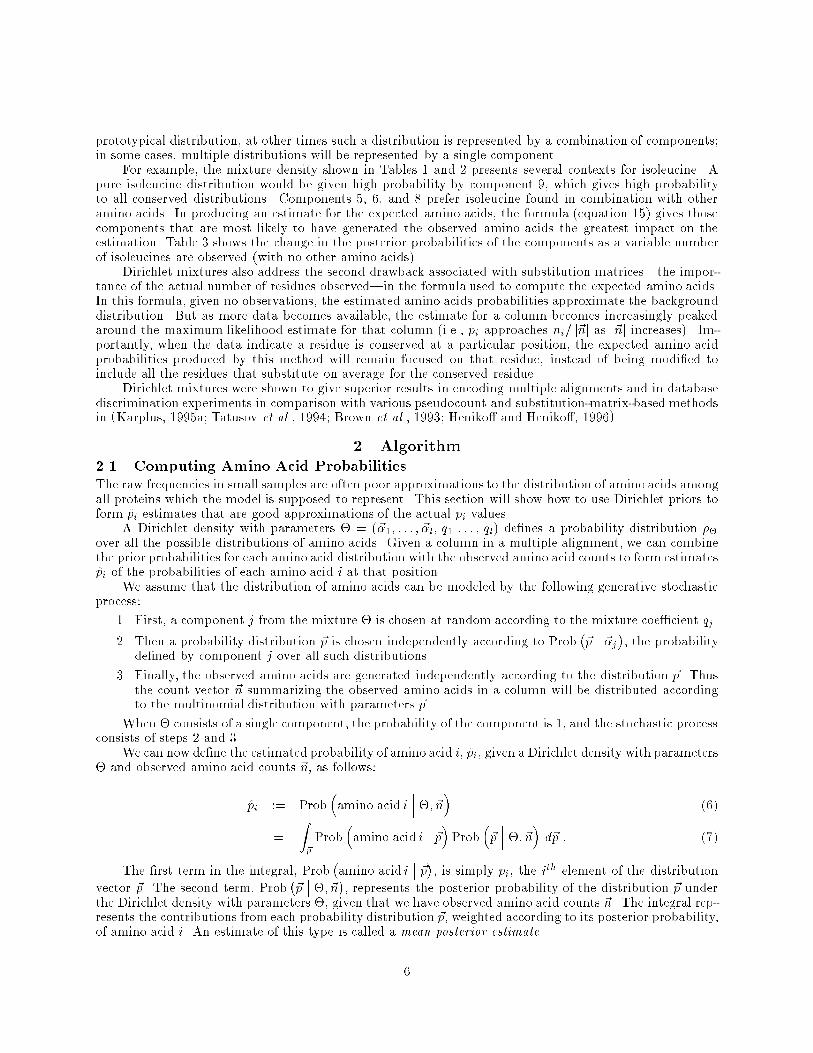
prototypical distribution, at other times such a distribution is represented by a combination of components;in some cases, multiple distributions will be represented by a single component.
For example, the mixture density shown in Tables 1 and 2 presents several contexts for isoleucine. Apure isoleucine distribution would be given high probability by component 9, which gives high probabilityto all conserved distributions. Components 5, 6, and 8 prefer isoleucine found in combination with otheramino acids. In producing an estimate for the expected amino acids, the formula (equation 15) gives thosecomponents that are most likely to have generated the observed amino acids the greatest impact on theestimation. Table 3 shows the change in the posterior probabilities of the components as a variable numberof isoleucines are observed (with no other amino acids).
Dirichlet mixtures also address the second drawback associated with substitution matrices|the impor-tance of the actual number of residues observed|in the formula used to compute the expected amino acids.In this formula, given no observations, the estimated amino acids probabilities approximate the backgrounddistribution. But as more data becomes available, the estimate for a column becomes increasingly peakedaround the maximum likelihood estimate for that column (i.e., p̂i approaches ni= j~nj as j~nj increases). Im-portantly, when the data indicate a residue is conserved at a particular position, the expected amino acidprobabilities produced by this method will remain focused on that residue, instead of being modi�ed toinclude all the residues that substitute on average for the conserved residue.
Dirichlet mixtures were shown to give superior results in encoding multiple alignments and in databasediscrimination experiments in comparison with various pseudocount and substitution-matrix-based methodsin (Karplus, 1995a; Tatusov et al., 1994; Brown et al., 1993; Heniko� and Heniko�, 1996).
2 Algorithm
2.1 Computing Amino Acid Probabilities
The raw frequencies in small samples are often poor approximations to the distribution of amino acids amongall proteins which the model is supposed to represent. This section will show how to use Dirichlet priors toform p̂i estimates that are good approximations of the actual pi values.
A Dirichlet density with parameters � = (~�1; : : : ; ~�l; q1 : : : ; ql) de�nes a probability distribution ��over all the possible distributions of amino acids. Given a column in a multiple alignment, we can combinethe prior probabilities for each amino acid distribution with the observed amino acid counts to form estimatesp̂i of the probabilities of each amino acid i at that position.
We assume that the distribution of amino acids can be modeled by the following generative stochasticprocess:
1. First, a component j from the mixture � is chosen at random according to the mixture coe�cient qj.
2. Then a probability distribution ~p is chosen independently according to Prob�~p�� ~�j�, the probability
de�ned by component j over all such distributions.
3. Finally, the observed amino acids are generated independently according to the distribution ~p. Thusthe count vector ~n summarizing the observed amino acids in a column will be distributed accordingto the multinomial distribution with parameters ~p.
When � consists of a single component, the probability of the component is 1, and the stochastic processconsists of steps 2 and 3.
We can now de�ne the estimated probability of amino acid i, p̂i, given a Dirichlet density with parameters� and observed amino acid counts ~n, as follows:
p̂i := Prob�amino acid i
��� �; ~n� (6)
=
Z~p
Prob�amino acid i
��� ~p�Prob�~p ��� �; ~n� d~p : (7)
The �rst term in the integral, Prob�amino acid i
�� ~p�, is simply pi, the ith element of the distribution
vector ~p. The second term, Prob�~p�� �; ~n�, represents the posterior probability of the distribution ~p under
the Dirichlet density with parameters �, given that we have observed amino acid counts ~n. The integral rep-resents the contributions from each probability distribution ~p, weighted according to its posterior probability,of amino acid i. An estimate of this type is called a mean posterior estimate.
6

2.1.1 Computing probabilities using a single density (pseudocounts)
In the case of a single-component density with parameters ~�, the mean posterior estimate of the probabilityof amino acid i is de�ned
p̂i :=
Z~p
Prob�amino acid i
��� ~p�Prob�~p ��� ~�; ~n� d~p : (8)
By Lemma 4 (the proof of which is found in the Appendix) the posterior probability of each distribution~p, given the count data ~n and the density with parameters ~�, is
Lemma 4:
Prob�~p��� ~�; ~n� = �(j~�j+ j~nj)Q20
i=1 �(�i + ni)
20Yi=1
p�i+ni�1i ;
where � is the Gamma function, the continuous generalization of the integer factorial function (i.e., �(x+1) =x!).
Here we can substitute pi for Prob�amino acid i
�� ~p� and the result of Lemma 4 into equation 8, giving
p̂i :=�(j~�j+ j~nj)Q20k=1 �(�k + nk)
Z~p
pi
20Yk=1
p�k+nk�1k d~p : (9)
Now, noting the contribution of the pi term within the integral, and using equation (47) from Lemma
2, givingR~p
Qi p
�i�1i d~p =
Qi�(�i)
�(j~�j) ; we have
p̂i :=�(j~�j+ j~nj)
�(j~�j+ j~nj+ 1)
�(�i + ni + 1)Q
k 6=i �(�k + nk)Q20k=1 �(�k + nk)
: (10)
Since �(n+1)�(n) = n!
(n�1)! = n, we obtain
p̂i :=
Z~p
piProb�~p��� ~�; ~n� d~p =
ni + �ij~nj+ j~�j
: (11)
The method in the case of a single Dirichlet density can thus be seen as adding a vector ~� of pseudocountsto the vector ~n of observed counts, and then normalizing so that
Pi p̂i = 1.
Note, when j~nj = 0, the estimate produced is simply �i= j~�j, the normalized values of the parameters ~�,which are the means of the Dirichlet density. While not necessarily the background frequency of the aminoacids in the training set, this mean is often a close approximation. Thus, in the absence of data, our estimateof the expected amino acid probabilities will be close to the background frequencies. The computationalsimplicity of the pseudocount method is one of the reasons Dirichlet densities are so attractive.
2.1.2 Computing probabilities using mixture densities
In the case of a mixture density, we compute the amino acid probabilities in a similar way:
p̂i := Prob�amino acid i
��� �; ~n� = Z~p
Prob�amino acid i
��� ~p�Prob�~p ��� �; ~n� d~p : (12)
As in the case of the single density, we can substitute pi for Prob(amino acid i j ~p). In addition, since �is a mixture of Dirichlet densities, by the de�nition of a mixture (equation 5), we can expand Prob(~p j�; ~n)obtaining
p̂i :=
Z~p
pi
0@ lX
j=1
Prob�~p��� ~�j; ~n�Prob�~�j ��� ~n;��
1A d~p : (13)
7

In this equation, Prob�~�j�� ~n;�� is the posterior probability of the jth component of the density, given
the vector of counts ~n (equation 16 below). It captures our assessment that the jth component was chosenin step 1 of the stochastic process generating these observed amino acids. The �rst term, Prob(~p j ~�j; ~n),then represents the probability of each distribution ~p, given component j and the count vector ~n.
Pulling out terms not depending on ~p from inside the integral gives us
p̂i :=lX
j=1
Prob�~�j
��� ~n;��Z~p
piProb(~p j ~�j; ~n) d~p : (14)
Substituting equation 11, 4
p̂i :=lX
j=1
Prob�~�j
��� ~n;�� ni + �j;ij~nj+ j~�jj
: (15)
Thus, instead of identifying one single component of the mixture that accounts for the observed data,we determine how likely each individual component is to have produced the data. Then, each componentcontributes pseudocounts proportional to the posterior probability that it produced the observed counts.This probability is calculated using Bayes' Rule:
Prob�~�j
��� ~n;�� = qj Prob�~n�� ~�j ; j~nj�
Prob�~n�� �; j~nj� : (16)
Prob�~n�� ~�j; j~nj� is the probability of the count vector ~n given the jth component of the mixture, and is
derived in Section A.3. The denominator, Prob�~n�� �; j~nj�, is de�ned
Prob�~n��� �; j~nj� = lX
k=1
qkProb�~n��� ~�k; j~nj� : (17)
Equation 15 reveals a smooth transition between reliance on the prior information, in the absence ofsu�cient data, and con�dence in the observed frequencies as the number of observations increases. Whenj~nj = 0, p̂i is simply
Pj qj�j;i= j~�jj, the weighted sum of the mean of each Dirichlet density in the mixture.
As the number of observations increases, the ni values dominate the �i values, and this estimate approachesthe maximum likelihood estimate, p̂i := ni= j~nj.
When a component has a very small j~�j, it adds a very small bias to the observed amino acid frequencies.Such components give high probability to all distributions peaked around individual amino acids. Theaddition of such a small bias allows these components to not shift the estimated amino acids away fromconserved distributions, even given relatively small numbers of observed counts.
By contrast, components having a larger j~�j tend to favor mixed distributions, that is, combinationsof amino acids. In these cases, the individual �j;i values tend to be relatively large for those amino acids ipreferred by the component. When such a component has high probability given a vector of counts, these�j;i have a corresponding in uence on the expected amino acids predicted for that position. The estimatesproduced may include signi�cant probability for amino acids not seen at all in the count vector underconsideration.
2.2 Estimation of Dirichlet Densities
In this section we give the derivation of the procedure to estimate the parameters of a mixture prior.Much statistical analysis has been done on amino acid distributions found in particular secondary structuralenvironments in proteins. However, our primary focus in developing these techniques for protein modelinghas been to rely as little as possible on previous knowledge and assumptions, and instead to use statisticaltechniques that uncover the underlying key information in the data. Consequently, instead of beginning withsecondary structure or other column labeling, our approach takes unlabeled training data (i.e., columns frommultiple alignments with no information attached) and attempts to discover those classes of distributions of
4Formula 15 was misreported in previous work (Brown et al., 1993; Karplus, 1995a; Karplus, 1995b).
8

amino acids that are intrinsic to the data. The statistical method directly estimates the most likely Dirichletmixture density through clustering observed counts of amino acids. In most cases, the common amino aciddistributions we �nd are easily identi�ed (e.g., aromatic residues), but we do not set out a priori to �nddistributions representing known environments.
As we will show, the case where the prior consists of a single density follows directly from the generalcase of a mixture. In the case of a mixture, we have two sets of parameters to estimate: the ~� parametersfor each component, and the q, or mixture coe�cient, for each component. In the case of a single density, weneed only estimate the ~� parameters. In our practice, we estimate these parameters in a two-stage process:�rst we estimate the ~�, keeping the mixture coe�cients q �xed, then we estimate the q, keeping the ~�parameters �xed. This two-stage process is iterated until all estimates stabilize.5
As the derivations that follow can become somewhat complex, we provide two tables in the Appendixto help the reader: Table 8 summarizes our notation, and Table 9 contains an index to key derivations andde�nitions.
Given a set of m columns from a variety of multiple alignments, we tally the frequency of each aminoacid in each column, with the end result being a vector of counts of each amino acid for each column in thedata set. Thus, our primary data is a set of m count vectors. Many multiple alignments of di�erent proteinfamilies are included, so m is typically in the thousands.
We have used Maximum Likelihood to estimate the parameters � from the set of count vectors; thatis, we seek those parameters that maximize the probability of occurrence of the observed count vectors.We assume the three-stage stochastic model described in Section 2.1 was used independently to generateeach of the count vectors in our observed set of count vectors. Under this assumption of independence, theprobability of the entire set of observed frequency count vectors is equal to the product of their individualprobabilities. Thus, we seek to �nd the model that maximizes
Qmt=1 Prob
�~nt�� �; j~ntj�. If we take the
negative logarithm of this quantity, we obtain the encoding cost of all the count vectors under the mixture.Since the encoding cost of the count vectors is inversely related to their probability, we can equivalently seeka mixture density with parameters � that minimizes the encoding cost
f(�) = �
mXt=1
logProb�~nt
��� �; j~ntj� : (18)
In the simplest case, we �x the number of components l in the Dirichlet mixture to a particular valueand then estimate the 21l � 1 parameters (twenty �i values for each of the components, and l � 1 mixturecoe�cients). In other experiments, we attempt to estimate l as well. The simplest method to estimate linvolves estimating several Dirichlet mixtures for each number of components, and choosing the smallestmixture that performs well enough for our purposes. Unfortunately, even for �xed l, there does not appearto be an e�cient method of estimating these parameters that is guaranteed to �nd the maximum likelihoodestimate. However, a variant of the standard estimation-maximization (EM) algorithm for mixture densityestimation works well in practice6. EM has been proved to result in closer and closer approximations to alocal optimumwith every iteration of the learning cycle; a global optimum, unfortunately, is not guaranteed(Dempster et al., 1977). Since there are many rather di�erent local optima with similar performance, nooptimization technique is likely to �nd the global optimum. The mixture described in Tables 1 and 2 is thebest local optimum we have found in many di�erent optimizations.
2.2.1 Deriving the ~� parameters
Since we require that the �i be strictly positive, and we want the parameters upon which we will do gradientdescent to be unconstrained, we reparameterize, setting �j;i = ewj;i , where wj;i is an unconstrained realnumber. Then, the partial derivative of f (equation 18) with respect to wj;i is
5This two-stage process is not necessary; we have also implemented an algorithm for mixture estimation thatoptimizes all parameters simultaneously. However, the performance of these mixtures is no better, and the math ismore complex.
6An introduction to this method of mixture density estimation is given in (Duda and Hart, 1973). We havemodi�ed their procedure to estimate a mixture of Dirichlet rather than Gaussian densities.
9

@f(�)
@wj;i= �
mXt=1
@ log Prob�~nt�� �; j~ntj�
@�j;i
@�j;i@wj;i
: (19)
We will use two lemmas in this section, the proofs for which are given in the Appendix:
Lemma 5:
@ log Prob�~n�� �; j~nj�
@�j;i= Prob
�~�j
��� ~n;�� @ log Prob�~n�� ~�j; j~nj�
@�j;i:
Lemma 6:
@ log Prob�~n�� ~�; j~nj�
@�i= (j~�j) �(j~nj+ j~�j) + (ni + �i) �(�i)
where (x) = �0(x)=�(x). Using Lemma 5, we obtain
@f(�)
@wj;i= �
mXt=1
Prob�~�j
��� ~nt;�� @ logProb�~nt�� ~�j; j~ntj�
@�j;i
@�j;i@wj;i
: (20)
Using Lemma 6, and the fact that @�j;i
@wj;i= �j;i, we obtain
@f(�)
@wj;i= �
mXt=1
�j;iProb�~�j
��� ~nt;���(j~�jj)� (j~ntj+ j~�jj) + (nt;i + �j;i)� (�j;i)�: (21)
To optimize the ~� parameters of the mixture, we do gradient descent on the weights ~w, taking a step inthe direction of the negative gradient (controlling the size of the step by the variable �, 0 < � � 1) duringeach iteration of the learning cycle. Thus, the gradient descent rule in the mixture case can now be de�nedas follows:
wnewj;i := wold
j;i � �@f(�)
@wj;i(22)
:= woldj;i + �
mXt=1
�j;iProb�~�j
��� ~nt;���(j~�jj)� (j~ntj+ j~�jj) + (nt;i + �j;i) �(�j;i)�:(23)
Now, letting Sj =Pm
t=1Prob�~�j�� ~nt;��, this gives us
wnewj;i := wold
j;i + � �j;i
Sj((j~�jj) �(�j;i)) +
mXt=1
Prob�~�j
��� ~nt;���(nt;i + �j;i)�(j~ntj+ j~�jj)�!
:
(24)
In the case of a single density, Prob(~� j~n;�) = 1 for all vectors ~n, thus Sj =Pm
t=1 Prob�~��� ~nt;�� = m,
and the gradient descent rule for a single density can be written as
wnewi := wold
i + � �i
m ((j~�j)� (�i)) +
mXt=1
�(nt;i + �i)� (j~ntj+ j~�j)
�!: (25)
After each update of the weights, the ~� parameters are reset, and the process continued until the changein the encoding cost (equation 18) falls below some pre-de�ned cuto�.
10

2.2.2 Mixture coe�cient estimation
In the case of a mixture of Dirichlet densities, the mixture coe�cients, q, of each component are alsoestimated. However, since we require that the mixture coe�cients must be non-negative and sum to 1,we �rst reparameterize, setting qj = Qj= jQj, where the Qj are constrained to be strictly positive, and
jQj =Pl
j=1Qj . As in the �rst stage, we want to maximize the probability of the data given the model,
which is equivalent to minimizing the encoding cost (equation 18). In this stage, we take the derivative off with respect to Qj. However, instead of having to take iterative steps in the direction of the negativegradient, as we did in the �rst stage, we can set the derivative to zero, and solve for those qj = Qj= jQj thatmaximize the probability of the data. As we will see, however, the new qj are a function of the previous qj;thus, this estimation process must also be iterated.
Taking the gradient of f with respect to Qj, we obtain
@f(�)
@Qj= �
mXt=1
@ logProb�~nt�� �; j~ntj�
@Qj: (26)
We introduce Lemma 8 (the proof for which is found in Section A.8),
Lemma 8:
@ logProb�~n�� �; j~nj�
@Qj=
Prob�~�j�� ~n;��
Qj�
1
jQj:
Using Lemma 8, we obtain
@f(�)
@Qj= �
mXt=1
Prob
�~�j�� ~nt;��
Qj�
1
jQj
!(27)
=m
jQj�
Pmt=1 Prob
�~�j�� ~nt;��
Qj: (28)
Since the gradient must vanish for those mixture coe�cients giving the maximum likelihood, we set thegradient to zero, and solve. Thus, the maximum likelihood setting for qj is
qj :=Qj
jQj(29)
:=1
m
mXt=1
Prob�~�j
��� ~nt;�� : (30)
Here, the reestimated mixture coe�cients7 are functions of the old mixture coe�cients, so we iteratethis process until the change in the encoding cost falls below the prede�ned cuto�.
In summary, when estimating the parameters of a mixture prior, we alternate between reestimatingthe ~� parameters of each density in the mixture, by gradient descent on the ~w, resetting �j;i = ewj;i aftereach iteration, followed by re-estimating and resetting the mixture coe�cients as described above, until theprocess converges.
3 ImplementationImplementing Dirichlet mixture priors for use in hidden Markov models or other stochastic models of bio-logical sequences is not di�cult, but there are many details that can cause problems if not handled carefully.
This section splits the implementation details into two groups: those that are essential for getting work-ing Dirichlet mixture code (Section 3.1), and those that increase e�ciency, but are not essential (Section 3.2).
7It is easy to con�rm that these coe�cients sum to 1, as required, sincePl
j=1
Pm
t=1Prob
�~�j�� ~nt;�� =Pm
t=1
Pl
j=1Prob
�~�j�� ~nt;�� =Pm
t=11 =m.
11

3.1 Essential details
In Section 2.1, we gave the formulas for computing the amino acid probabilities in the cases of a singledensity (equation 11) and of a mixture density (equation 15).
For a single Dirichlet component, the estimation formula is trivial:
p̂i :=ni + �ij~nj+ j~�j
; (31)
and no special care is needed in the implementation. For the case of a multi-component mixture, theimplementation is not quite so straightforward.
As we showed in the derivation of equation 15,
p̂i :=lX
j=1
Prob�~�j
��� ~n;�� ni + �j;ij~nj+ j~�jj
: (32)
The interesting part for computation comes in computing Prob�~�j�� ~n;�� (see equation 16). We can
expand Prob�~n�� �; j~nj� using equation 17 to obtain
Prob�~�j
��� ~n;�� = qjProb�~n�� ~�j; j~nj�Pl
k=1 qkProb�~n�� ~�k; j~nj� : (33)
Note that this is a simple normalization of qjProb�~n�� ~�j; j~nj� to sum to one. Rather than carry the
normalization through all the equations, we can work directly with Prob�~n�� ~�j; j~nj�, and put everything
back together at the end.First, we can expand Prob
�~n�� ~�j; j~nj� using Lemma 3 (the proof of which is found in Section A.3):
Prob�~n��� ~�j; j~nj� = �(j~nj+ 1)�(j~�jj)
�(j~nj+ j~�jj)
20Yi=1
�(ni + �j;i)
�(ni + 1)�(�j;i): (34)
If we rearrange some terms, we obtain
Prob�~n��� ~�j; j~nj� =
Q20i=1 �(ni + �j;i)
�(j~nj+ j~�jj)
�(j~�jj)Q20i=1 �(�j;i)
�(j~nj+ 1)Q20i=1 �(ni + 1)
: (35)
The �rst two terms are most easily expressed using the Beta function: B(x) =Q20
i=1 �(xi)=�(j~xj), where,as usual, j~xj =
Pi xi. This simpli�es the expression to
Prob�~n��� ~�j; j~nj� = B (~n+ ~�j)
B (~�j)
�(j~nj+ 1)Q20i=1 �(ni + 1)
: (36)
The remaining Gamma functions are not easily expressed with a Beta function, but they don't need tobe. Since they depend only on ~n and not on j, when we do the normalization to make the Prob
�~�j�� ~n;��
sum to one, this term will cancel out, giving us
Prob�~�j
��� ~n;�� = qjB(~n+~�j )B(~�j )Pl
k=1 qkB(~n+~�k)B(~�k)
: (37)
Plugging this formula into equation 32 gives us
p̂i :=
Plj=1 qj
B(~n+~�j)B(~�j)
ni+�j;i
j~nj+j~�jjPlk=1 qk
B(~n+~�k)B(~�k)
: (38)
Since the denominator of equation 38 is independent of i, we can compute p̂i by normalizing
Xi =lX
j=1
qjB(~n+ ~�j)
B(~�j)
ni + �j;ij~nj+ j~�jj
(39)
12

to sum to one. That is,
p̂i =XiP20k=1Xk
: (40)
The biggest problem that implementors run into is that these Beta functions can get very large or verysmall|outside the range of the oating-point representation of most computers. The obvious solution is towork with the logarithm of the Beta function:
logB(x) = log
Qi � (x(i))
� (j~xj)
=Xi
log � (x(i)) � log � (j~xj) :
Most libraries of mathematical routines include the lgamma function which implements log �(x), and so usingthe logarithm of the Beta function is not di�cult.
We could compute each Xi using only the logarithmic notation, but it turns out to be slightly moreconvenient to use the logarithms just for the Beta functions:
Xi =lX
j=1
qjB(~�j + ~n)
B(~�j)
�j;i + nij~�jj+ j~nj
=lX
j=1
qje(logB(~�j+~n)�logB(~�j)) �j;i + ni
j~�jj+ j~nj:
Some care is needed in the conversion from the logarithmic representation back to oating-point, sincethe ratio of the Beta functions may be so large or so small that it cannot be represented as oating-pointnumbers. Luckily, we do not really need to compute Xi, only p̂i = Xi=
P20k=1Xk. This means that we
can divide Xi by any constant and the normalization will eliminate the constant. Equivalently, we canfreely subtract a constant (independent of j and i) from logB(~�j + ~n)� logB(~�j) before converting back to oating-point. If we choose the constant to be maxj (logB(~�j + ~n)� logB(~�j)), then the largest logarithmicterm will be zero, and all the terms will be reasonable.8
3.2 E�ciency improvements
The previous section gave simple computation formulas for p̂i (equations 39 and 40). When computations ofp̂i are done infrequently (for example, for pro�les, where p̂i only needs to be computed once for each columnof the pro�le), those equations are perfectly adequate.
When recomputing p̂i frequently, as may be done in a Gibbs sampling program or training a hiddenMarkov model, it is better to have a slightly more e�cient computation. Since most of the computationtime is spent in the lgamma function used for computing the log Beta functions, the biggest e�ciency gainscome from avoiding the lgamma computations.
If we assume that the �j;i and qj values change less often than the values for ~n (which is true of almostevery application), then it is worthwhile to precompute logB(~�j), cutting the computation time almost inhalf.
If the ni values are mainly small integers (0 is common in all the applications we've looked at), then itis worth pre-computing log�(�j;i), log �(�j;i + 1), log �(�j;i + 2), and so on, out to some reasonable value.Precomputation should also be done for log�(j~�jj), log�(j~�jj+ 1), log�(j~�jj+ 2), and so forth. If all the ~nvalues are small integers, this precomputation almost eliminates the lgamma function calls.
In some cases, it may be worthwhile to build a special-purpose implementation of log �(x) that cachesall calls in a hash table, and does not call lgamma for values of x that it has seen before. Even larger savingsare possible when x is close to previously computed values, by using interpolation rather than calling lgamma.
8We could still get oating-point under ow to zero for some terms, but the p̂ computation will still be about asgood as can be done within oating-point representation.
13

4 DiscussionThe methods employed to estimate and use Dirichlet mixture priors are shown to be �rmly based onBayesian statistics. While biological knowledge has been introduced only indirectly from the multiplealignments used to estimate the mixture parameters, the mixture priors produced agree with acceptedbiological understanding. The e�ectiveness of Dirichlet mixtures for increasing the ability of statisticalmodels to recognize homologous sequences has been demonstrated experimentally in (Brown et al., 1993;Tatusov et al., 1994; Karplus, 1995a; Bailey and Elkan, 1995; Wang et al., 1996; Heniko� and Heniko�, 1996;Hughey and Krogh, 1996).
The mixture priors we have estimated thus far have been on unlabeled multiple alignment columns|columns with no secondary structure or other information attached. Previous work deriving structurallyinformed distributions, such as that by L�uthy, McLachlan, and Eisenberg (L�uthy et al., 1991), has beenshown to increase the accuracy of pro�les in both database search and multiple alignment by enablingthem to take advantage of prior knowledge of secondary structure (Bowie et al., 1991). However, thesedistributions cannot be used in a Bayesian framework, since there is no measure of the variance associatedwith each distribution, and Bayes' rule requires that the observed frequency counts be modi�ed inverselyproportional to the variance in the distribution. Thus, to use these structural distributions one must assign avariance arbitrarily. We plan to estimate Dirichlet mixtures for particular environments, and to make thesemixtures available on the World-Wide Web.
Dirichlet mixture priors address two primary weaknesses of substitution matrices: considering only therelative frequency of the amino acids while ignoring the actual number of amino acids observed, and having�xed substitution probabilities for each amino acid. One of the potentially most problematic consequencesof these drawbacks is that substitution matrices do not produce estimates that are conserved, or mostlyconserved, where the evidence is clear that an amino acid is conserved. The method presented here correctsthese problems. When little data is available, the amino acids predicted are those that are known to beassociated in di�erent contexts with the amino acids observed. As the available data increases, the aminoacid probabilities produced by this method converge to the observed frequencies in the data. In particular,when evidence exists that a particular amino acid is conserved at a given position, the expected amino acidestimates re ect this preference.
Because of the sensitivity of Dirichlet mixtures to the number of observations, any signi�cant correlationamong the sequences must be handled carefully. One way to compensate for sequence correlation is by the useof a sequence weighting scheme (Sibbald and Argos, 1990; Thompson et al., 1994a; Thompson et al., 1994b;Heniko� and Heniko�, 1996). Dirichlet mixtures interact with sequence weighting in two ways. First,sequence weighting changes the expected distributions somewhat, making mixed distributions more uniform.Second, the total weight allotted the sequences plays a critical role when Dirichlet densities are used. If thedata is highly correlated, and this is not compensated for in the weighting scheme (by reducing the totalcounts), the estimated amino acid distributions will be too close to the raw frequencies in the data, andnot generalized to include similar residues. Since most sequence weighting methods are concerned onlywith relative weights, and pay little attention to the total weight allotted the sequences, we are developingsequence weighting schemes that coordinate the interaction of Dirichlet mixtures and sequence weights.
Since the mixture presented in this paper was estimated and tested on alignments of fairly close homologs(the BLOCKS (Heniko� and Heniko�, 1991) and HSSP (Sander and Schneider, 1991) alignment databases),it may not accurately re ect the distributions we would expect frommore remote homologs. We are planningto train a Dirichlet mixture speci�cally to recognize true remote homologies, by a somewhat di�erent trainingtechnique on a database of structurally aligned sequences.
Finally, as the detailed analysis of Karplus (Karplus, 1995a; Karplus, 1995b) shows, the Dirichlet mix-tures already available are close to optimal as far as their capacity for assisting in computing estimates ofamino acid distributions, given a single-column context, and assuming independence between columns andbetween sequences for a given column. Thus, further work in this area will perhaps pro�t by focusing onobtaining information from relationships among the sequences (for instance, as revealed in a phylogenetictree) or in inter-columnar interactions.
The Dirichlet mixture prior from Table 1 is available electronically at our World-Wide Web sitehttp://www.cse.ucsc.edu/research/compbio/. In addition to the extensions described above, we plan tomake programs for using and estimating Dirichlet mixture densities available on our World-Wide Web andftp sites later this year. See our World-Wide Web site for announcements.
14

AcknowledgmentsWe gratefully acknowledge the input and suggestions of Stephen Altschul, Tony Fink, Lydia Gregoret, Stevenand Jorja Heniko�, Graeme Mitchison, and Chris Sander. Richard Lathrop made numerous suggestions thatimproved the quality of the manuscript greatly, as did the anonymous referees. Special thanks to friendsat Laforia, Universit�e de Pierre et Marie Curie, in Paris, and the Biocomputing Group at the EuropeanMolecular Biology Laboratory at Heidelberg, who provided workstations, support, and scienti�c inspirationduring the early stages of writing this paper. This work was supported in part by NSF grants CDA-9115268, IRI-9123692, and BIR-9408579; DOE grant 94-12-048216, ONR grant N00014-91-J-1162, NIHgrant GM17129, a National Science Foundation Graduate Research Fellowship, and funds granted by theUCSC Division of Natural Sciences. The Sanger Centre is supported by the Wellcome Trust. This paper isdedicated to the memory of Tal Grossman, a dear friend and a true mensch.
15

ReferencesAltschul, Stephen F.; Gish, Warren; Miller, Webb; Meyers, Eugene W.; and Lippman, David J. 1990. Basic localalignment search tool. JMB 215:403{410.
Altschul, Stephen F. 1991. Amino acid substitution matrices from an information theoretic perspective. JMB219:555{565.
Asai, K.; Hayamizu, S.; and Onizuka, K. 1993. HMM with protein structure grammar. In Proceedings of the HawaiiInternational Conference on System Sciences, Los Alamitos, CA. IEEE Computer Society Press. 783{791.
Bailey, Timothy L. and Elkan, Charles 1995. The value of prior knowledge in discovering motifs with MEME. InISMB-95, Menlo Park, CA. AAAI/MIT Press. 21{29.
Baldi, P. and Chauvin, Y. 1994. Smooth on-line learning algorithms for hidden Markov models. Neural Computation6(2):305{316.
Baldi, P.; Chauvin, Y.; Hunkapiller, T.; and McClure, M. A. 1992. Adaptive algorithms for modeling and analysisof biological primary sequence information. Technical report, Net-ID, Inc., 8 Cathy Place, Menlo Park, CA 94305.
Barton, G. J. and Sternberg, M. J. 1990. Flexible protein sequence patterns: A sensitive method to detect weakstructural similarities. JMB 212(2):389{402.
Berger, J. 1985. Statistical Decision Theory and Bayesian Analysis. Springer-Verlag, New York.
Bernardo, J.M. and Smith, A.F.M. 1994. Bayesian Theory. John Wiley and Sons, �rst edition.
Bowie, J. U.; L�uthy, R.; and Eisenberg, D. 1991. A method to identify protein sequences that fold into a knownthree-dimensional structure. Science 253:164{170.
Brown, M. P.; Hughey, R.; Krogh, A.; Mian, I. S.; Sj�olander, K.; and Haussler, D. 1993. Using Dirichlet mixturepriors to derive hidden Markov models for protein families. In Hunter, L.; Searls, D.; and Shavlik, J., editors 1993,ISMB-93, Menlo Park, CA. AAAI/MIT Press. 47{55.
Bucher, Philipp; Karplus, Kevin; Moeri, Nicolas; and Ho�man, Kay 1996. A exible motif search technique basedon generalized pro�les. Computers and Chemistry 20(1):3{24.
Churchill, G. A. 1989. Stochastic models for heterogeneous DNA sequences. Bull Math Biol 51:79{94.
Claverie, Jean-Michael 1994. Some useful statistical properties of position-weight matrices. Computers and Chem-
istry 18(3):287{294.
Dempster, A. P.; Laird, N. M.; and Rubin, D. B. 1977. Maximum likelihood from incomplete data via the EM
algorithm. J. Roy. Statist. Soc. B 39:1{38.
Doolittle, R. F. 1986. Of URFs and ORFs: A primer on how to analyze derived amino acid sequences. UniversityScience Books, Mill Valley, California.
Duda, R. O. and Hart, P. E. 1973. Pattern Classi�cation and Scene Analysis. Wiley, New York.
Eddy, S.R.; Mitchison, G.; and Durbin, R. 1995. Maximum discrimination hidden Markov models of sequenceconsensus. J. Comput. Biol. 2:9{23.
Eddy, Sean 1995. Multiple alignment using hidden Markov models. In ISMB-95, Menlo Park, CA. AAAI/MITPress. 114{120.
Eddy, S.R. 1996. Hidden markov models. Current Opinions in Structural Biology.
George, David G.; Barker, Winona C.; and Hunt, Lois T. 1990. Mutation data matrix and its uses. Methods in
Enzymology 183:333{351.
Gradshteyn, I. S. and Ryzhik, I. M. 1965. Table of Integrals, Series, and Products. Academic Press, fourth edition.
Gribskov, Michael; McLachlan, Andrew D.; and Eisenberg, David 1987. Pro�le analysis: Detection of distantlyrelated proteins. PNAS 84:4355{4358.
Gribskov, M.; L�uthy, R.; and Eisenberg, D. 1990. Pro�le analysis. Methods in Enzymology 183:146{159.
Heniko�, Steven and Heniko�, Jorja G. 1991. Automated assembly of protein blocks for database searching. NAR19(23):6565{6572.
Heniko�, Steven and Heniko�, Jorja G. 1992. Amino acid substitution matrices from protein blocks. PNAS
89:10915{10919.
Heniko�, Steven and Heniko�, Jorja G. 1993. Performance evaluation of amino acid substitution matrices. Proteins:Structure, Function, and Genetics 17:49{61.
Heniko�, Jorja G. and Heniko�, Steven 1996. Using substitution probabilities to improve position-speci�c scoringmatrices. CABIOS.
Heniko�, Steven; Wallace, James C.; and Brown, Joseph P. 1990. Finding protein similarities with nucleotidesequence databases. Methods in Enzymology 183:111{132.
16

Hughey, Richard and Krogh, Anders 1996. Hidden Markov models for sequence analysis: Extension and analysis ofthe basic method. CABIOS 12(2):95{107.
Jones, David T.; Taylor, William R.; and Thornton, Janet M. 1992. The rapid generation of mutation data matricesfrom protein sequences. CABIOS 8(3):275{282.
Karplus, Kevin 1995a. Regularizers for estimating distributions of amino acids from small samples. In ISMB-95,Menlo Park, CA. AAAI/MIT Press.
Karplus, Kevin 1995b. Regularizers for estimating distributions of amino acids from small samples. Technical ReportUCSC-CRL-95-11, University of California, Santa Cruz. URL ftp://ftp.cse.ucsc.edu/pub/tr/ucsc-crl-95-11.ps.Z.
Krogh, A.; Brown, M.; Mian, I. S.; Sj�olander, K.; and Haussler, D. 1994. Hidden Markov models in computationalbiology: Applications to protein modeling. JMB 235:1501{1531.
L�uthy, R.; McLachlan, A. D.; and Eisenberg, D. 1991. Secondary structure-based pro�les: Use of structure-conserving scoring table in searching protein sequence databases for structural similarities. Proteins: Structure,Function, and Genetics 10:229{239.
Nowlan, S. 1990. Maximum likelihood competitive learning. In Touretsky, D., editor 1990, Advances in Neural
Information Processing Systems, volume 2. Morgan Kaufmann. 574{582.
Rodionov, Michael A. and Johnson, Mark S. 1994. Residue-residue contact substitution probabilities derived fromaligned three-dimensional structures and the identi�cation of common folds. Protein Science 3:2366{2377.
Sander, C. and Schneider, R. 1991. Database of homology-derived protein structures and the structural meaning ofsequence alignment. Proteins 9(1):56{68.
Santner, T. J. and Du�y, D. E. 1989. The Statistical Analysis of Discrete Data. Springer Verlag, New York.
Sibbald, P. and Argos, P. 1990. Weighting aligned protein or nucleic acid sequences to correct for unequal repre-sentation. JMB 216:813{818.
Stultz, C. M.; White, J. V.; and Smith, T. F. 1993. Structural analysis based on state-space modeling. Protein
Science 2:305{315.
Tatusov, Roman L.; Altschul, Stephen F.; and Koonin, Eugen V. 1994. Detection of conserved segments in proteins:Iterative scanning of sequence databases with alignment blocks. PNAS 91:12091{12095.
Thompson, Julie D.; Higgins, Desmond G.; and Gibson, Toby J. 1994a. Improved sensitivity of pro�le searchesthrough the use of sequence weights and gap excision. CABIOS 10(1):19{29.
Thompson, Julie D.; Higgins, Desmond G.; and Gibson, Toby J. 1994b. CLUSTAL W: Improving the sensitivityof progressive multiple sequence alignment through sequence weighting, position-speci�c gap penalties, and weightmatrix choice. NAR 22(22):4673{4680.
Wang, Jason T. L.; Marr, Thomas G.; Shasha, Dennis; Shapiro, Bruce; Chirn, Gung-Wei; and Lee, T. Y. 1996.Complementary classi�cation approaches for protein sequences. Protein Engineering.
Waterman, M. S. and Perlwitz, M. D. 1986. Line geometries for sequence comparisons. Bull. Math. Biol. 46:567{577.
White, James V.; Stultz, Collin M.; and Smith, Temple F. 1994. Protein classi�cation by stochastic modeling andoptimal �ltering of amino-acid sequences. Mathematical Biosciences 119:35{75.
17

5 Tables
Parameters of Dirichlet mixture prior Blocks9
Comp. 1 Comp. 2 Comp. 3 Comp. 4 Comp. 5 Comp. 6 Comp. 7 Comp. 8 Comp. 9q 0.1829 0.0576 0.0898 0.0792 0.0831 0.0911 0.1159 0.0660 0.2340j~�j 1.1806 1.3558 6.6643 2.0814 2.0810 2.5681 1.7660 4.9876 0.0995A 0.2706 0.0214 0.5614 0.0701 0.0411 0.1156 0.0934 0.4521 0.0051C 0.0398 0.0103 0.0454 0.0111 0.0147 0.0373 0.0047 0.1146 0.0040D 0.0175 0.0117 0.4383 0.0194 0.0056 0.0124 0.3872 0.0624 0.0067E 0.0164 0.0108 0.7641 0.0946 0.0102 0.0181 0.3478 0.1157 0.0061F 0.0142 0.3856 0.0873 0.0131 0.1536 0.0517 0.0108 0.2842 0.0034G 0.1319 0.0164 0.2591 0.0480 0.0077 0.0172 0.1058 0.1402 0.0169H 0.0123 0.0761 0.2149 0.0770 0.0071 0.0049 0.0497 0.1003 0.0036I 0.0225 0.0353 0.1459 0.0329 0.2996 0.7968 0.0149 0.5502 0.0021K 0.0203 0.0139 0.7622 0.5766 0.0108 0.0170 0.0942 0.1439 0.0050L 0.0307 0.0935 0.2473 0.0722 0.9994 0.2858 0.0277 0.7006 0.0059M 0.0153 0.0220 0.1186 0.0282 0.2101 0.0758 0.0100 0.2765 0.0014N 0.0482 0.0285 0.4415 0.0803 0.0061 0.0145 0.1878 0.1185 0.0041P 0.0538 0.0130 0.1748 0.0376 0.0130 0.0150 0.0500 0.0974 0.0090Q 0.0206 0.0230 0.5308 0.1850 0.0197 0.0113 0.1100 0.1266 0.0036R 0.0236 0.0188 0.4655 0.5067 0.0145 0.0126 0.0386 0.1436 0.0065S 0.2161 0.0291 0.5834 0.0737 0.0120 0.0275 0.1194 0.2789 0.0031T 0.0654 0.0181 0.4455 0.0715 0.0357 0.0883 0.0658 0.3584 0.0036V 0.0654 0.0361 0.2270 0.0425 0.1800 0.9443 0.0254 0.6617 0.0029W 0.0037 0.0717 0.0295 0.0112 0.0127 0.0043 0.0032 0.0615 0.0027Y 0.0096 0.4196 0.1210 0.0287 0.0264 0.0167 0.0187 0.1993 0.0026
Table 1: Parameters of Mixture Prior Blocks9This table contains the parameters de�ning a nine-component mixture prior estimated on unweighted columns fromthe Blocks database. The �rst row gives the mixture coe�cient (q) for each component. The second row gives thej~�j =
Pi�i for each component. Rows A (alanine) through Y (tyrosine) contain the values of each of the components'
~� parameters for that amino acid. Section 1.4 gives details on how to interpret these values.
It is informative to examine this table and Table 2 in unison. The mixture coe�cients (q) of the densities reveal thatin this mixture, the components peaked around the aromatic and the uncharged hydrophobic residues (components2 and 8) represent the smallest fraction of the columns used to train the mixture, and the component representingall the highly conserved residues (component number 9) represents the largest fraction of the data captured by anysingle component.
Examining the j~�j of each component shows that the two components with the largest values of j~�j (and so the mostmixed distributions) represent the polars (component 3) and the uncharged hydrophobics (component 8), respectively.The component with the smallest j~�j (component 9) gives probability to pure distributions.
This mixture prior is available via anonymous ftp at our ftp site, ftp://ftp.cse.ucsc.edu/pub/protein/dirichlet/and at our World-Wide Web site http://www.cse.ucsc.edu/research/compbio/dirichlet.html.
18

Analysis of 9-Component Dirichlet Mixture Prior Blocks9
Comp. Ratio (r) of amino acid frequency relative to background frequency8 � r 4 � r � 8 2 � r � 4 1 � r � 2 1=2 � r < 1 1=4 � r < 1=2 1=8 � r < 1=4 r < 1=8
1 SAT CGP NVM QHRIKFLDW EY2 Y FW H LM NQICVSR TPAKDGE3 QE KNRSHDTA MPYG VLIWCF4 KR Q H NETMS PWYALGVCI DF5 LM I FV WYCTQ APHR KSENDG6 IV LM CTA F YSPWN EQKRDGH7 D EN QHS KGPTA RY MVLFWIC8 M IVLFTYCA WSHQRNK PEG D9 PGW CHRDE NQKFYTLAM SVI
Table 2: Preferred amino acids of Blocks9
The function used to compute the ratio of the frequency of amino acid i in component j relative to the
background frequency predicted by the mixture as a whole is �j;i=j~�jjPkqk�k;i=j~�kj
.
An analysis of the amino acids favored by each component reveals the following:
Component 1 favors small neutral residues.
Component 2 favors the aromatics.
Component 3 gives high probability to most of the polar residues (except for C, Y, and W).
Component 4 gives high probability to positively charged amino acids and residues with NH2 groups.
Component 5 gives high probability to residues that are aliphatic or large and non-polar.
Component 6 prefers I and V (aliphatic residues commonly found in Beta sheets), and allows substitutionswith L and M.
Component 7 gives high probability to negatively charged residues, allowing substitutions with certain ofthe hydrophilic polar residues.
Component 8 gives high probability to uncharged hydrophobics, with the exception of glycine.
Component 9 gives high probability to distributions peaked around individual amino acids (especially P,G, W, and C).
19

Posterior probability of the components of Dirichlet mixture Blocks9 given 1-10 isoleucines# Ile Comp. 1 Comp. 2 Comp. 3 Comp. 4 Comp. 5 Comp. 6 Comp. 7 Comp. 8 Comp. 912345678910
0.00 0.25 0.50 0.75 1.00
Table 3: The posterior probability of each component in Dirichlet mixture Blocks9 (equation 16) given1 to 10 isoleucines. Initially, component 6, which prefers I and V found jointly, is most likely, followed bycomponents 5 and 8, which like aliphatic residues in general. As the number of observed isoleucines increases,component 9, which favors pure distributions of any type, increases in probability, but component 6 remainsfairly probable. The more mixed distributions get increasingly unlikely as the number of observed isoleucinesincreases.
20

Method used to estimate amino acid probabilities given 1 isoleucineSubstitution Matrices Pseudocount Dirichlet MixtureBlosum62 SM-Opt. PC-Opt. Blocks9
A 0.055 0.028 0.046 0.037C 0.018 0.008 0.010 0.010D 0.020 0.006 0.026 0.008E 0.020 0.011 0.031 0.012F 0.044 0.025 0.021 0.027G 0.022 0.011 0.033 0.012H 0.010 0.005 0.014 0.006I 0.253 0.517 0.495 0.472
K 0.027 0.011 0.031 0.014L 0.147 0.117 0.046 0.117
M 0.037 0.026 0.017 0.030N 0.017 0.009 0.025 0.010P 0.018 0.008 0.018 0.008Q 0.016 0.008 0.023 0.010R 0.019 0.010 0.027 0.012S 0.027 0.015 0.039 0.020T 0.048 0.025 0.033 0.028V 0.171 0.146 0.042 0.149
W 0.006 0.003 0.006 0.004Y 0.024 0.011 0.017 0.013
Table 4: Estimated amino acid probabilities using various methods, given one isoleucine.
Tables 4, 5, 6 and 7 give amino acid probability estimates produced by di�erent methods, given a varyingnumber of isoleucines observed (and no other amino acids). Methods used to estimate these probabilitiesinclude two substitution matrices: Blosum62, which does Gribskov average score (Gribskov et al., 1987)using the Blosum-62 matrix (Heniko� and Heniko�, 1992), and SM-Opt, which does matrix multiply withmatrix optimized for the Blocks database (Karplus, 1995a); one pseudocount method, PC-Opt, which is asingle-component Dirichlet density optimized for the Blocks database (Karplus, 1995a); and the Dirichletmixture Blocks9, the nine-component Dirichlet mixture given in Tables 1 and 2.
In order to interpret the changing amino acid probabilities produced by the Dirichlet mixture, Blocks9, werecommend examining this table in conjunction with Table 3. Table 3 shows the changing contribution ofthe components in the mixture as the number of isoleucines increases. In the estimate produced by theDirichlet mixture, isoleucine has probability just under 0:5 when a single isoleucine is observed, and theother aliphatic residues have signi�cant probability. This reveals the in uence of components 5 and 6, withtheir preference for allowing substitutions with valine, leucine and methionine. By ten observations, thenumber of isoleucines observed dominates the pseudocounts added for other amino acids, and the amino acidestimate is peaked around isoleucine.
The pseudocount method PC-opt also converges to the observed frequencies in the data, as the number ofisoleucines increases, but does not give any signi�cant probability to the other aliphatic residues when thenumber of isoleucines is small.
By contrast, the substitution matrices give increased probability to the aliphatic residues, but the estimatedprobabilities remain �xed as the number of isoleucines increases.
21
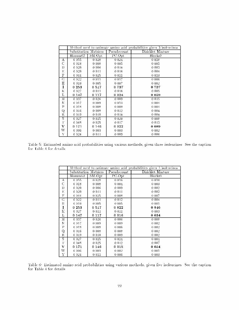
Method used to estimate amino acid probabilities given 3 isoleucinesSubstitution Matrices Pseudocount Dirichlet MixtureBlosum62 SM-Opt. PC-Opt. Blocks9
A 0.055 0.028 0.024 0.018C 0.018 0.008 0.005 0.005D 0.020 0.006 0.014 0.003E 0.020 0.011 0.016 0.004F 0.044 0.025 0.011 0.013G 0.022 0.011 0.017 0.006H 0.010 0.005 0.007 0.002I 0.253 0.517 0.737 0.737
K 0.027 0.011 0.016 0.005L 0.147 0.117 0.024 0.059
M 0.037 0.026 0.009 0.015N 0.017 0.009 0.013 0.004P 0.018 0.008 0.009 0.004Q 0.016 0.008 0.012 0.004R 0.019 0.010 0.014 0.004S 0.027 0.015 0.020 0.008T 0.048 0.025 0.017 0.013V 0.171 0.146 0.022 0.089
W 0.006 0.003 0.003 0.002Y 0.024 0.011 0.009 0.006
Table 5: Estimated amino acid probabilities using various methods, given three isoleucines. See the captionfor Table 4 for details.
Method used to estimate amino acid probabilities given 5 isoleucinesSubstitution Matrices Pseudocount Dirichlet MixtureBlosum62 SM-Opt. PC-Opt. Blocks9
A 0.055 0.028 0.016 0.010C 0.018 0.008 0.004 0.003D 0.020 0.006 0.009 0.002E 0.020 0.011 0.011 0.002F 0.044 0.025 0.008 0.007G 0.022 0.011 0.012 0.004H 0.010 0.005 0.005 0.001I 0.253 0.517 0.822 0.846
K 0.027 0.011 0.011 0.003L 0.147 0.117 0.016 0.034
M 0.037 0.026 0.006 0.008N 0.017 0.009 0.009 0.002P 0.018 0.008 0.006 0.002Q 0.016 0.008 0.008 0.002R 0.019 0.010 0.009 0.002S 0.027 0.015 0.014 0.004T 0.048 0.025 0.012 0.007V 0.171 0.146 0.015 0.054
W 0.006 0.003 0.002 0.001Y 0.024 0.011 0.006 0.003
Table 6: Estimated amino acid probabilities using various methods, given �ve isoleucines. See the captionfor Table 4 for details.
22

Method used to estimate amino acid probabilities given 10 isoleucinesSubstitution Matrices Pseudocount Dirichlet Mixture
Blosum62 Blocks-Opt. Blocks-Opt. Blocks9A 0.055 0.028 0.009 0.004C 0.018 0.008 0.002 0.001D 0.020 0.006 0.005 0.001E 0.020 0.011 0.006 0.001F 0.044 0.025 0.004 0.003G 0.022 0.011 0.006 0.002H 0.010 0.005 0.003 0.001I 0.253 0.517 0.902 0.942
K 0.027 0.011 0.006 0.001L 0.147 0.117 0.009 0.012
M 0.037 0.026 0.003 0.003N 0.017 0.009 0.005 0.001P 0.018 0.008 0.003 0.001Q 0.016 0.008 0.005 0.001R 0.019 0.010 0.005 0.001S 0.027 0.015 0.008 0.002T 0.048 0.025 0.006 0.003V 0.171 0.146 0.008 0.020
W 0.006 0.003 0.001 0.001Y 0.024 0.011 0.003 0.001
Table 7: Estimated amino acid probabilities using various methods, given ten isoleucines. See the captionfor Table 4 for details.
23

A Appendix
j~xj =P
ixi, where ~x is any vector.
~n = n1; : : : ; n20 is a vector of counts from a column in a multiple alignment. The symbol ni refers to thenumber of amino acids i in the column. The tth such observation in the data is denoted ~nt.
~p = (p1; : : : ; p20),P
pi = 1, pi � 0, are the parameters of the multinomial distributions from which the ~nare drawn.
P is the set of all such ~p.
~� = (�1; : : : ; �20) s.t. �i > 0, are the parameters of a Dirichlet density. The parameters of the jth
component of a Dirichlet mixture are denoted ~�j. The symbol �j;i refers to the ith parameter of the
jth component of a mixture.
qj = Prob(~�j) is the mixture coe�cient of the jth component of a mixture.
� = (q1; : : : ; ql; ~�1; : : : ; ~�l) = all the parameters of the Dirichlet mixture.
~w = (w1; : : : ; w20), are weight vectors, used during gradient descent to train the Dirichlet density parameters~�. After each training cycle, �j;i is set to ewj;i . The symbol wj;i is the value of the i
th parameter ofthe jth weight vector. The nomenclature weights comes from arti�cial neural networks.
m = the number of columns from multiple alignments used in training.
l = the number of components in a mixture.
� = eta, the learning rate used to control the size of the step taken during each iteration of gradient descent.
Table 8: Summary of notation.
24

f(�) = �Pm
t=1log(Prob
�~nt�� �; j~ntj�) (18)
(the encoding cost of all the count vectors given the mixture|the function minimized)
�(j~nj + 1) = n! (for integer n � 0) (43)(Gamma function)
(x) = @ log �(x)@x
= �0(x)�(x) (64)
(Psi function)
Prob�~n�� ~p; j~nj� = �(j~nj+ 1)
Q20
i=1
pnii
�(ni+1)(44)
(the probability of ~n under the multinomial distribution with parameters ~p)
Prob�~n�� ~�; j~nj� = �(j~nj+1) �(j~�j)
�(j~nj+j~�j)
Q20
i=1�(ni+�i)
�(ni+1)�(�i)(51)
(the probability of ~n under the Dirichlet density with parameters ~�)
Prob�~n�� �; j~nj� =
Pl
k=1qk Prob(~n j ~�k; j~nj) (17)
(the probability of ~n given the entire mixture prior)
Prob�~�j�� ~n;�� =
qj Prob(~n j ~�j ;j~nj)
Prob�~n
���;j~nj� (16)
(shorthand for the posterior probability of the jth component of the mixturegiven the vector of counts ~n)
Table 9: Index to key derivations and de�nitions.
25

A.1 Lemma 1. Prob (~n j ~p; j~nj) = �(j~nj+ 1)Q20
i=1pnii
�(ni+1)
Proof:
For a given vector of counts ~n, with pi being the probability of seeing the ith amino acid, and j~nj =P
ini,
there are j~nj!n1!n2!:::n20 !
distinct permutations of the amino acids which result in the count vector ~n. If we allow for
the simplifying assumption that each amino acid is generated independently (i.e., the sequences in the alignment are
uncorrelated), then each such permutation has probabilityQ20
i=1 pnii . Thus, the probability of a given count vector ~n
given the multinomial parameters ~p is
Prob�~n
��� ~p; j~nj� =j~nj!
n1!n2! : : : n20!
20Yi=1
pnii (41)
= j~nj!
20Yi=1
pniini!
: (42)
To enable us to handle real-valued data (such as that obtained from using a weighting scheme on the sequencesin the training set), we introduce the Gamma function, the continuous generalization of the integer factorial function,
�(n+ 1) = n! : (43)
Substituting the Gamma function, we obtain the equivalent form
Prob�~n
��� ~p; j~nj� = �(j~nj+ 1)
20Yi=1
pnii�(ni + 1)
: (44)
26

A.2 Lemma 2. Prob (~p j ~�) = �(j~�j)Q20
i=1�(�i)
Q20i=1 p
�i�1i
Proof:
Under the Dirichlet density with parameters ~�, the probability of the distribution ~p (where pi � 0, andP
ipi = 1)
is de�ned as follows:
Prob(~p j ~�) =
Q20
i=1 p�i�1iR
~p2P
Qip�i�1i d~p
: (45)
We introduce two formulas concerning the Beta function|its de�nition (Gradshteyn and Ryzhik, 1965, p. 948)
B(x; y) =
Z 1
0
tx�1(1� t)y�1 dt
=�(x)�(y)
�(x+ y);
and its combining formula (Gradshteyn and Ryzhik, 1965, p. 285)Z b
0
tx�1(b� t)y�1 dt = bx+y�1B(x;y) :
This allows us to write the integral over all ~p vectors as a multiple integral, rearrange some terms, and obtainZ~p2P
Yi
p�i�1i d~p = B(�1; �2 + : : :+ �20)B(�2; �3 + : : :+ �20) : : :B(�19; �20) (46)
=
Qi�(�i)
�(j~�j): (47)
We can now give an explicit de�nition of the probability of the amino acid distribution ~p given the Dirichletdensity with parameters ~�:
Prob(~p j ~�) =�(j~�j)Q20
i=1�(�i)
20Yi=1
p�i�1i : (48)
27
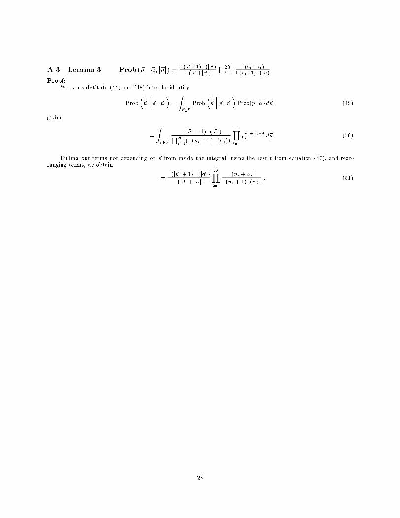
A.3 Lemma 3. Prob (~n j ~�; j~nj) = �(j~nj+1)�(j~�j)�(j~nj+j~�j)
Q20i=1
�(ni+�i)�(ni+1)�(�i)
Proof:
We can substitute (44) and (48) into the identity
Prob�~n
��� ~�; j~nj� =
Z~p2P
Prob�~n
��� ~p; j~nj�Prob(~p j ~�)d~p; (49)
giving
=
Z~p2P
�(j~nj+ 1)�(j~�j)Q20
i=1(�(ni + 1) �(�i))
20Yi=1
pni+�i�1i d~p : (50)
Pulling out terms not depending on ~p from inside the integral, using the result from equation (47), and rear-ranging terms, we obtain
=�(j~nj+ 1) �(j~�j)
�(j~nj+ j~�j)
20Yi=1
�(ni + �i)
�(ni + 1)�(�i): (51)
28

A.4 Lemma 4. Prob (~p j ~�;~n) = �(j~�j+j~nj)Q20
i=1�(�i+ni)
Q20i=1 p
�i+ni�1i
Proof:
By repeated application of the rule for conditional probability, the probability of the distribution ~p, given theDirichlet density with parameters ~�, and the observed amino acid count vector ~n is de�ned
Prob�~p
��� ~�; ~n� =Prob
�~p; ~�; ~n
�� j~nj�Prob
�~�; ~n
�� j~nj� (52)
=Prob
�~n�� ~p; ~�; j~nj�Prob(~p; ~�)
Prob�~n�� ~�; j~nj�Prob(~�) (53)
=Prob
�~n�� ~p; ~�; j~nj�Prob �~p �� ~��Prob
�~n�� ~�; j~nj� : (54)
However, once the point ~p is �xed, the probability of ~n no longer depends on ~�. Hence,
Prob�~p
��� ~�; ~n� = Prob�~n�� ~p; j~nj�Prob �~p �� ~��
Prob�~n�� ~�; j~nj� : (55)
At this point, we apply the results from previous derivations for quantities Prob�~n�� ~p; j~nj� (equation 44),
Prob�~p�� ~�� (equation 48), and Prob
�~n�� ~�; j~nj� (equation 51). This gives us
Prob�~p
��� ~�; ~n� =
��(j~nj+1)Qi�(ni+1)
Qipnii
���(j~�j)Qi�(�i)
Qip�i�1i
��(j~nj+ j~�j)
Qi�(ni + 1)�(�i)
�(j~nj+ 1) �(j~�j)Q
i�(ni + �i)
: (56)
Most of the terms cancel, and we have
Prob�~p
��� ~�; ~n� =�(j~�j+ j~nj)Q20
i=1�(�i + ni)
20Yi=1
p�i+ni�1i : (57)
Note that this is the expression for a Dirichlet density with parameters ~�+ ~n. This property, that the posteriordensity of � is from the same family as the prior, characterizes all conjugate priors, and is one of the properties thatmake Dirichlet densities so attractive.
29

A.5 Lemma 5.@ log Prob
�~nj�;j~nj
�@�j;i
= Prob (~�j j ~n;�)@ log Prob
�~nj~�j;j~nj
�@�j;i
Proof:
The derivative with respect to �j;i of the log likelihood of each count vector ~n given the mixture is
@ log Prob�~n�� �; j~nj�
@�j;i=
1
Prob�~n�� �; j~nj�
@Prob�~n�� �; j~nj�
@�j;i: (58)
Applying equation 17, this gives us
@ log Prob�~n�� �; j~nj�
@�j;i=
1
Prob�~n�� �; j~nj�
@PL
k=1qk Prob
�~n�� ~�k; j~nj�
@�j;i: (59)
Since the derivative of Prob�~n�� ~�k; j~nj� with respect to �j;i is zero for all k 6= j, and the mixture coe�cients
(the qk) are independent parameters, this yields
@ log Prob�~n�� �; j~nj�
@�j;i=
qj
Prob�~n�� �; j~nj�
@Prob�~n�� ~�j; j~nj�
@�j;i: (60)
We rearrange equation (16) somewhat, and replace qj=Prob�~n�� �; j~nj� by its equivalent, obtaining
@ log Prob�~n�� �; j~nj�
@�j;i=
Prob�~�j�� ~n;��
Prob�~n�� ~�j; j~nj�
@Prob�~n�� ~�j; j~nj�
@�j;i: (61)
Here, again using the fact that @ log(f(x))@x
= 1f(x)
@f(x)@x
, we obtain the �nal form
@ log Prob�~n�� �; j~nj�
@�j;i= Prob
�~�j
��� ~n;�� @ log Prob�~n�� ~�j; j~nj�
@�j;i: (62)
30

A.6 Lemma 6.@ log Prob
�~nj~�;j~nj
�@�i
= (j~�j)� (j~nj+ j~�j) + (ni + �i)�(�i)
Proof:
In this proof, we use Lemma 3 giving
Prob�~n
��� ~�; j~nj� =�(j~nj+ 1)�(j~�j)
�(j~nj+ j~�j)
20Yi=1
�(ni + �i)
�(ni + 1)�(�i):
Since the derivative of terms not depending on �i are zero, we obtain that for a single vector of counts ~n,
@ log Prob�~n�� ~�; j~nj�
@�i=
@ log �(j~�j)
@�i�
@ log �(j~nj+ j~�j)
@�i+
@ log �(ni + �i)
@�i�
@ log �(�i)
@�i: (63)
Now, if we substitute the shorthand
(x) =@ log �(x)
@x=
�0(x)
�(x); (64)
we have@ log Prob
�~n�� ~�; j~nj�
@�i= (j~�j)�(j~nj+ j~�j) + (ni + �i)�(�i) : (65)
31

A.7 Lemma 7.@Prob
�~nj�;j~nj
�@Qi
=Prob
�~nj~�i;j~nj
��Prob
�~nj�;j~nj
�jQj
Proof:
Substituting equation (17), giving Prob�~n�� �; j~nj� =Pl
j=1qj Prob(~n j ~�j; j~nj) and replacing qj by Qj= jQj, we
obtain
@Prob�~n�� �; j~nj�
@Qi
=@Pl
j=1(Qj= jQj)Prob
�~n�� ~�j; j~nj�
@Qi
: (66)
As the derivative of a sum is the sum of the derivatives, we can use the standard product rule for di�erentiation,and obtain
@Prob�~n�� �; j~nj�
@Qi
=
lXj=1
(Qj= jQj)
@Prob�~n�� ~�j; j~nj�
@Qi
+Prob�~n
��� ~�j; j~nj� @(Qj= jQj)
@Qi
!: (67)
Since@Prob
�~n
��~�j ;j~nj�@Qi
= 0 for all j, this gives us
@Prob�~n�� �; j~nj�
@Qi
=
lXj=1
Prob�~n
��� ~�j; j~nj� @(Qj= jQj)
@Qi
: (68)
Taking the derivative of the fraction (Qj= jQj) with respect to Qi, we obtain
@(Qj= jQj)
@Qi
= jQj�1 @Qj
@Qi
+Qj
@ jQj�1
@Qi
: (69)
The �rst term, jQj�1 @Qj
@Qi, is zero when j 6= i, and is 1
jQj when j = i. The second term, Qj@jQj�1
@Qi, is simply
�Qj
jQj2.
Thus, this gives us
@Prob�~n�� �; j~nj�
@Qi
=Prob
�~n�� ~�i; j~nj�jQj
�
lXj=1
Prob�~n
��� ~�j; j~nj� Qj
jQj2: (70)
Here, qj = Qj= jQj allows us to replace Qj= jQj2 with qj= jQj, giving us
=Prob
�~n�� ~�i; j~nj��Pl
j=1 qjProb�~n�� ~�j; j~nj�
jQj: (71)
At this point, we use equation 17 and obtain
@Prob�~n�� �; j~nj�
@Qi
=Prob
�~n�� ~�i; j~nj�� Prob
�~n�� �; j~nj�
jQj: (72)
32

A.8 Lemma 8.@ logProb
�~nj�;j~nj
�@Qj
=Prob
�~�jj~n;�
�Qj
� 1jQj
Proof:
Using Lemma 7, we can derive
@ log Prob�~n�� �; j~nj�
@Qj
=1
Prob�~n�� �; j~nj�
@Prob�~n�� �; j~nj�
@Qj
(73)
=1
Prob�~n�� �; j~nj�
Prob�~n�� ~�j; j~nj�� Prob
�~n�� �; j~nj�
jQj(74)
=
Prob
�~n�� ~�j; j~nj�
Prob�~n�� �; j~nj� � 1
!= jQj : (75)
If we rearrange equation 16, we obtainProb
�~n
��~�j ;j~nj�Prob
�~n
���;j~nj� =Prob(~�j j ~n;�)
qj. This allows us to write
@ log Prob�~n�� �; j~nj�
@Qj
=
�Prob(~�j j ~n;�)
qj� 1
�= jQj : (76)
Now we can use the identity qj = Qj= jQj, obtaining the equivalent
@ log Prob�~n�� �; j~nj�
@Qj
=Prob
�~�j�� ~n;��
Qj
�1
jQj: (77)
33