POLICY RESEARCH WORKING PAPER 28 06

Dirty Exports and EnvironmentalRegulation

Do Standards Matter to Trade?

John S. Wilson

Tsunehiro Otsuki

Mirvat Sewadeb

The World Bank

Development Research Group

Trade

March 2002

Pub

lic D

iscl

osur

e A

utho

rized

Pub

lic D

iscl

osur

e A

utho

rized

Pub

lic D

iscl

osur

e A

utho

rized

Pub

lic D

iscl

osur

e A

utho

rized

| POLICY RESEARCH WORKING PAPER 2806

AbstractHow to address the link between environmental are regressed on factor endowments and measures ofregulation and trade was an important part of environmental standards (legislation in force). Thediscussions at the World Trade Organization Ministerial results suggest that, if country heterogeneity such asin Doha, Qatar in November 2001. Trade ministers enforcement of environmental regulations is controlledagreed to launch negotiations on trade and the for, more stringent environmental standards imply lowerenvironment, specifically clarification of WTO rules. net exports of metal mining, nonferrous metals, iron,

Wilson, Otsuki, and Sewadeh address an important and steel and chemicals. The authors find find that apart of the background context for deciding whether or trade agreement on a common environmental standardhow to link trade agreements to the environment from a will cost a non-OECD country substantially more thandeveloping country perspective. The authors ask whether an OECD country. Developing countries will, onenvironmental regulations affect exports of pollution- average, reduce exports of the five pollution-intensiveintensive or "dirty" goods in 24 countries between 1994 products by 0.37 percent of GNP. This represents 11and 1998. Based on a Heckscher-Ohlin-Vanek (HOV) percent of annual exports of these products from the 24model, net exports in five pollution-intensive industries studied countries.

This paper-a product of Trade, Development Research Group-is part of a larger effort in the group to explore the linkbetween standards, development, and trade. Copies of the paper are available free from the World Bank, 1818 H StreetNW, Washington, DC 20433. Please contact Paulina Flewitt, room MC3-333, telephone 202-473-2724, fax 202-522-1159, email address pflewitt@Caworldbank.org. Policy Research Working Papers are also posted on the Web at http://econ.worldbank.org. The authors may be contacted at jswilson@aworldbank.org, totsuki@aworldbank.org, ormsewadehC@worldbank.org. March 2002. (33 pages)

The Policy Research Working Paper Series disseminates the findings of work in progress to encourage the exchange of ideas aboutdevelopment issues. An objective of the series is to get the findings out quickly, even if the presentations are less than fully polished. Thepapers carry the names of the authors and should he cited accordingly. The findings, interpretations, and conclusions expressed in thispaper are entirely those of the authors. They do not necessarily represent the view of the World Bank, its Executive Directors, or thecountries they represent.

Produced by the Research Advisory Staff

Dirty Exports and Environmental Regulation:

Do Standards Matter to Trade?

John S. Wilson *,aTsunehiro Otsuki bMirvat Sewadeh

March 2002

abc Development Research Group (DECRG), The World Bank

JEL Classification: F18, 013, 019

'Corresponding author: Tsunehiro Otsuki, E-mail address: totsukigworldbank.org, Address: 1818 H

Street NW, Washington DC 20433, USA, Phone number: (202) 473-8095, Fax number: (202) 522-

1159. The authors are grateful for the useful comments from attendees at a World Bank Trade

Seminar held on June 19, 2001. The authors are also grateful for assistance provided by Baishali

Majumdar and Robert Simms.

1. Introduction

The relationship between environmental standards and trade is at the forefront of

policy debate. Disputes over linkages between trade and the environment have

intensified over the past decade. The 1999 Seattle Ministerial of the World Trade

Organization (WTO) ended in failure, at least in part, due to profound differences

over tying environmental performance to competitiveness in exports. The issue of

whether to link trade agreements to environmental standards was one of the factors

for consideration at the WTO Ministerial in November 2001 in Doha, Qatar. There

are only weak disciplines currently in the WTO agreements regarding environmental

standards, as reflected in the Marrakech decision on trade and environment. The

Technical Barriers to Trade Agreement and the Agreement on Sanitary and

Phytosanitary Standards both include provisions related to environmental protection,

however, there have been few formal disputes that were brought to the WTO. The

question remains whether trade agreements are the best policy tool to affect change in

environmental policy.'

If lax environmental standards provide additional incentives for export

competition in pollution-intensive industries, and if developing countries do not place

an emphasis on domestic environmental quality, then free trade may result in a "race

to the bottom" in regulation. Private sector firms may exert pressure on governments

in developed countries to scale back the most stringent environmental standards.

Alternatively, if developed countries seek to harmonize environmental standards

' For a more detailed discussion of these issues see: Global Economic Prospects and the Developing

Countries 2001, chapter 3, The World Bank, December 2000.

2

globally at increasingly high levels, then developing countries may confront lower

growth rates of exports in pollution-intensive industries.

This paper empirically explores the link between trade and environmental

standards by controlling for human capital as a technological variable. We also

explicitly include a measure of the degree of enforcement of environmental

regulations in the modeling. This enforcement mechanism is assumed to have a

distinct role from environmental legislation in the analysis.

We study major pollution-intensive industries: metal mining, nonferrous

metals, pulp and paper, iron and steel, and chemicals in 6 OECD and 18 non-OECD

countries over the period 1994 to 1998. The analysis in large part follows the

Hecksher-Ohlin-Vanek (HOV) model developed for econometric estimation by

Tobey (1990), using data on environmental stringency from Dasgupta et al. (2001).

This paper is organized as follows: Section 2 reviews the existing theoretical

and empirical works on trade and environmental regulation. Section 3 discusses the

common and distinct characteristics of the pollution-intensive industries. Section 4

reviews the existing cross-country measures of the stringency of environmental

regulation. Section 5 presents the data and the analytical framework. Section 6 reports

the results, and Section 7 analyzes the results and their implication on trade policy.

2. Trade and Environmental Regulation

Most studies that trace the link between trade and the stringency of an environmental

standard explore either the industrial flight (pollution-haven) or industrial

specialization hypothesis. The industrial flight hypothesis centers on investigating the

3

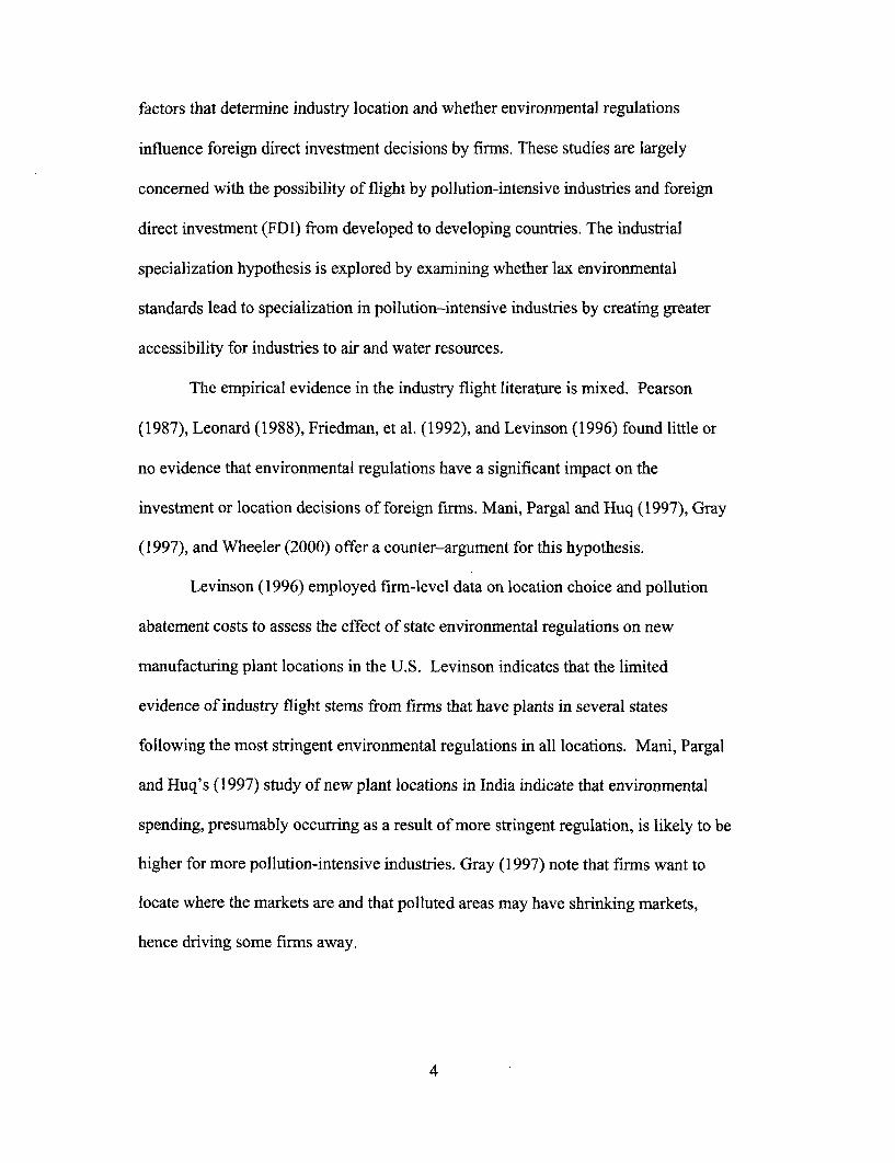
factors that determine industry location and whether environmental regulations

influence foreign direct investment decisions by firms. These studies are largely

concerned with the possibility of flight by pollution-intensive industries and foreign

direct investment (FDI) from developed to developing countries. The industrial

specialization hypothesis is explored by examining whether lax environmental

standards lead to specialization in pollution-intensive industries by creating greater

accessibility for industries to air and water resources.

The empirical evidence in the industry flight literature is mixed. Pearson

(1987), Leonard (1988), Friedman, et al. (1992), and Levinson (1996) found little or

no evidence that environmental regulations have a significant impact on the

investment or location decisions of foreign firms. Mani, Pargal and Huq (1997), Gray

(1997), and Wheeler (2000) offer a counter--argument for this hypothesis.

Levinson (1996) employed firm-level data on location choice and pollution

abatement costs to assess the effect of state environmental regulations on new

manufacturing plant locations in the U.S. Levinson indicates that the limited

evidence of industry flight stems from firms that have plants in several states

following the most stringent environmental regulations in all locations. Mani, Pargal

and Huq's (1997) study of new plant locations in India indicate that environmental

spending, presumably occurring as a result of more stringent regulation, is likely to be

higher for more pollution-intensive industries. Gray (1997) note that firms want to

locate where the markets are and that polluted areas may have shrinking markets,

hence driving some firms away.

4

On the contrary, Lucas et al. (1990) and List and Co (1999) found some

support for the industry-flight hypothesis. Lucas et al. suggest that implementation of

progressively strict environmental regulations in the OECD countries have led to

significant location displacement of pollution-intensive industries. List and Co study

show that regulatory expenditures per manufacturer and the location decision of a

new firm are inversely related in West Virginia.

Smarzynska and Wei (2001) also find some support for the industry-flight

hypothesis. They control for corruption levels in a host country and use a firm level

dataset for 25 transition economies to assess support for the industry flight

hypothesis. Wheeler (2000) provides examples of the link between air pollution

regulation and FDI in Mexico, Brazil, India, and the U.S. that illustrate the

importance of community, or firm level efforts, to internalize the costs of pollution in

developing countries.

The majority of studies that examine industrial specialization have found little

or no empirical support (Tobey, 1990; Low and Yeats, 1992; Grossman and Krueger,

1993; Xu, 1999). Tobey (1990) investigates whether domestic environmental

regulations have an impact on international trade patterns in five pollution-intensive

industries for 23 countries. He found no statistical significance of his environmental

regulation measures on the net exports of these industries. Grossman and Krueger

(1993) find no evidence that a comparative advantage is being created by lax

environmental regulations in Mexico. Xu (1999)'s study on bilateral trade found no

evidence that a country with stricter environmental standards lowering their total

exports of pollution-intensive goods.

5

Low and Yeats (1992) found that pollution-intensive industries account for a

large and growing share of exports in the total manufacture of exports in some

developing countries, and a decreasing share of exports in developed countries

between 1965 and 1988. Grossman and Krueger argue that the difficulty in finding

and supporting statistical evidence for the industrial specialization hypothesis lies in

the fact that endowments such as physical and human capital, and investment remain

dominant in determining a county's trade pattern.

On the contrary, Kalt (1988) finds that environmental regulations in the U.S.

have led to a sharp reduction in net manufacturing exports in 1977 presumably due to

a shift of output mix toward the production of clean air and water, and away from

pollution-intensive outputs. In contrast, Antweiler et al. (1998) suggests that trade

changes the composition of national output in a more polluting way for capital-

abundant countries. This implies that the developed countries have comparative

advantage in producing pollution-intensive goods.

3. Pollution-Intensive Industries

Various definitions have been used for pollution-intensive industries in the empirical

literature. Grossman and Krueger (1993) measure environmental intensity by using

the ratio of pollution abatement costs to the total amount of value added to a specific

U.S. industry. Low and Yeats (1992), and Xu (1999) define pollution-intensive

goods as products of industries that incurred abatement costs in the U.S. of

approximately 1 percent or more of the total value of sales in 1988. This definition

results in four industries: Iron and Steel, Metal Manufactures, Cement, and

6

Agricultural Chemicals. Smarzynska and Wei (2001) include in their analysis a set of

pollution-intensive industries, which range from the low to high level of pollution.

While the Smarzynska and Wei approach appears to be the most general in nature a

certain level of aggregation is useful when the impact of environmental standards is

compared across industries. Tobey defines pollution-intensive industries, as "those

whose direct and indirect abatement costs in the U.S. are equal to or greater than 1.85

percent of total costs." According to the author, 1.85 percent is used, because it

results-when commodities are aggregated-in a set of five industries that are

generally considered the polluting: Metal Mining, Primary Nonferrous Metals, Pulp

and Paper, Primary Iron and Steel, and Chemicals.

As there appears to be no definitive criteria yet adopted to define pollution

intensive, we follow Tobey's definition of pollution-intensive industries in our

analysis for comparison purposes. These five industries aggregate three-digit SITC

industries in the following manner:

Metal Mining: SITC (Revision 1) 281, 283

Primary Nonferrous Metals2: 681, 682, 683, 684, 685, 686, 687, 689

Pulp and Paper: 251, 641, 642

Primary Iron and Steel: 671, 672, 673, 674, 675, 676, 677, 678

Chemicals3 : 512, 513, 514, 581

2 Tables 2 and 3 contain all of the relevant information about nonferrous metals.

3 We added the Organic Chemicals industry to the Chemicals industry category, as it is also considered

to be pollution-intensive.

7

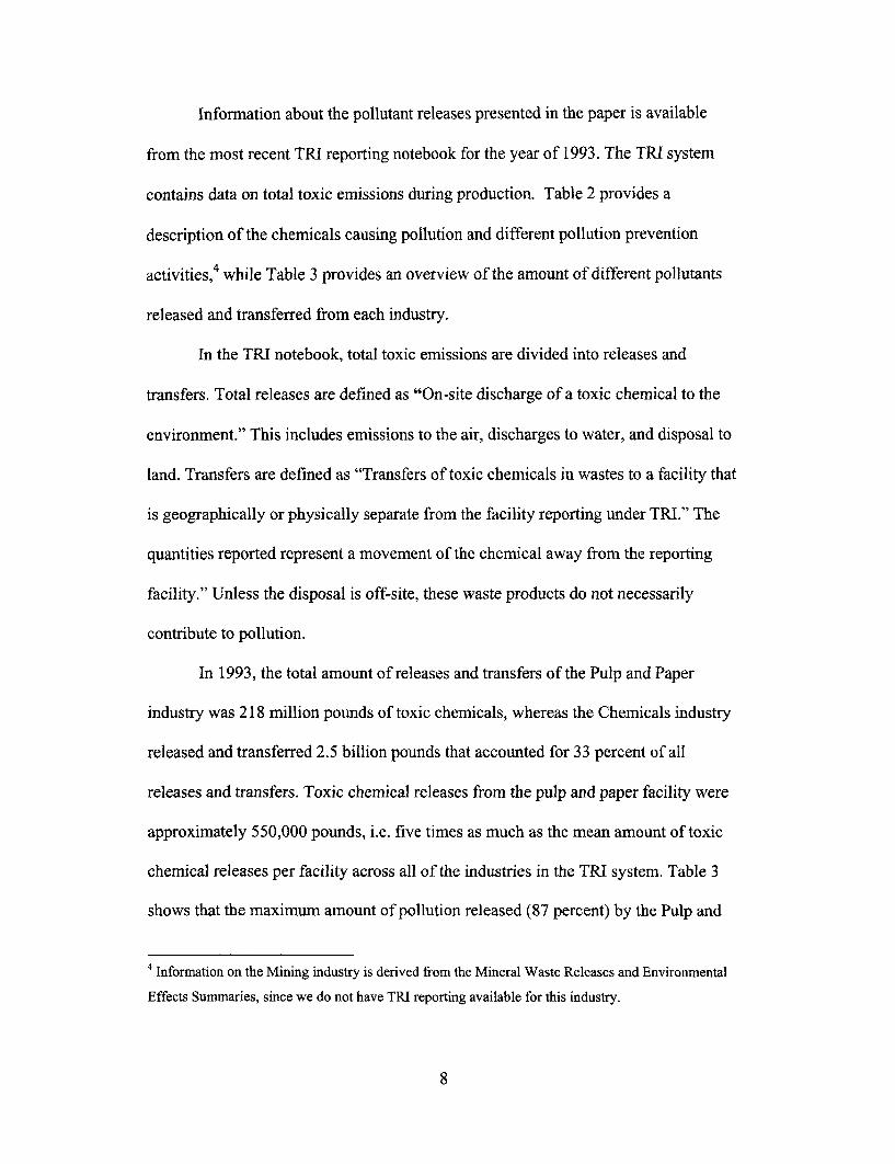
Information about the pollutant releases presented in the paper is available

from the most recent TRI reporting notebook for the year of 1993. The TRI system

contains data on total toxic emissions during production. Table 2 provides a

description of the chemicals causing pollution and different pollution prevention

activities,4 while Table 3 provides an overview of the amount of different pollutants

released and transferred from each industry.

In the TRI notebook, total toxic emissions are divided into releases and

transfers. Total releases are defined as "On-site discharge of a toxic chemical to the

environment." This includes emissions to the air, discharges to water, and disposal to

land. Transfers are defined as "Transfers of toxic chemicals in wastes to a facility that

is geographically or physically separate from the facility reporting under TRI." The

quantities reported represent a movement of the chemical away from the reporting

facility." Unless the disposal is off-site, these waste products do not necessarily

contribute to pollution.

In 1993, the total amount of releases and transfers of the Pulp and Paper

industry was 218 million pounds of toxic chemicals, whereas the Chemicals industry

released and transferred 2.5 billion pounds that accounted for 33 percent of all

releases and transfers. Toxic chemical releases from the pulp and paper facility were

approximately 550,000 pounds, i.e. five times as much as the mean amount of toxic

chemical releases per facility across all of the industries in the TRI system. Table 3

shows that the maximum amount of pollution released (87 percent) by the Pulp and

4 Information on the Mining industry is derived fiom the Mineral Waste Releases and Environmental

Effects Summaries, since we do not have TRI reporting available for this industry.

8

Paper industry is emitted to the air, followed by approximately 10 percent of as water

discharge.

A total of 438 million pounds of toxic chemicals were released and transferred

by the Organic Chemical industry, representing 18 percent of the total releases and

transfers by the entire chemical industry, and 6 percent of the releases and transfers

by all the industries under TRI. In comparison, releases and transfers by the Inorganic

Chemical industry totaled 249.7 million pounds in 1993. The Plastics industry

releases were mainly air pollutants. The Chemicals industry comprises the Organic,

Inorganic and Plastics industries. Historically, the Chemicals industries surpassed the

other industries in TRI chemical releases. Emissions to the air, and discharges to

water, are very significant in the Chemicals industry.

The Iron and Steel industry released and transferred a total of approximately

695 million pounds of pollutants containing a large proportion of metal-bearing

wastes. About 70 percent of these wastes are transferred for offsite recycling in order

to recover the metal content that results in increase in transfers in this industry.

Waste disposal on land represents a very large proportion from the total releases of

the Iron and Steel industry. When the transfers of different industries are compared,

the Iron and Steel industry appears to have a very high amount of pollutants relative

to the other industries. Moreover, emissions to the air and discharges to water are

significantly lower than land disposal. The bulk of industrial wastes from the Iron and

Steel industry are recycled.

9

4. Measuring Environmental Standards

It is essential to choose a reliable measure of an environmental standard. List and Co

(1999) use four different measures of the stringency of environmental regulation for

the U.S. The first two measures estimate money spent by different agencies within a

state to control air and water pollution and solid waste disposal. The third measure

they use is firm-level pollution abatement operating expenditures relative to abating

air and water pollution and solid waste disposal. The fourth measure is an index that

combines local, state and federal government pollution abatement efforts with firm-

level abatement expenditures to assign a dollar-value ranking to each state. A higher

value in the index implies more stringent environmental regulations. Tobey (1990) on

the other hand, measures environmental stringency by using data from a 1976

UNCTAD survey. The degree of environmental stringency is measured from one to

seven. Higher values imply more stringent regulations. Levinson (1996) includes six

different measures of environmental stringency in his study. These measures are: (1)

the Conservation Foundation index that measures each state's "effort to provide a

quality environment for citizens" (Duerksen, 1983); (2) the FREE (Fund for

Renewable Energy and the Environment) index, which measures the strength of state

environmental programs; (3) the Green index which is an aggregate measure of the

number of statutes that each state has from a list of 50 common environmental laws;

(4) monitoring employment that measures the states' efforts and abilities in enforcing

statutes; (5) aggregate abatement costs that show aggregate pollution abatement

operating costs across industries deflated by the number of production workers in the

state in 1982, and finally; (6) industry abatement costs which measure the amount the

10

manufacturers are required to pay for pollution abatement in each state, provided that

the characteristics of the manufacturer remain unchanged. Smarzynska and Wei

(2001) measure environmental standards by a country's participation in international

treaties (e.g. Convention on Long-range Transboundary Air Pollution), the quality of

ambient air, water and emission standards, and finally observed actual reduction in

various pollutants.

We use a cross-country index of the stringency in environmental regulation

developed by Dasgupta et al. (2001) for our analysis. A higher score in this index

reflects more stringent environmental standards. The authors randomly selected 31

UNCED reports from a total of 145. These 31 countries range from highly

industrialized, to extremely poor. Based on these reports, they conducted a survey

that considered the state of policy and performance in four environmental

dimensions: air, water, land, and living resources. We analyzed the apparent state of

policy as it affects the interactions between these four environmental dimensions and

five activity categories: agriculture, manufacture, energy, transport, and the urban

sector. Although many overlaps undoubtedly exist, we attempt to draw a separate

assessment for the interaction of each activity category with each environmental

dimension.

The Dasgupta survey employed 25 questions to categorize (1) the state of

environmental awareness, (2) the scope of legislation enacted, and (3) the control

mechanisms for enviromnental enforcement in place in each country. Environmental

awareness in the Dasgupta survey is a measurement of a country's level of public

concern about environmental quality. The legislation category of the Dasgupta

11

survey measures the extent to which a country's environmental legislation provides

broad protection of natural resources - such as protection of air, water, land, and

other resources. A control mechanism for environmental enforcement measures the

ability of regulators to enforce legislation. It reflects the history of environmental

regulation, existence of regulating institutions and infrastructure, and power given to

regulating agencies in each country.5

Due to its multi-dimensional property, the elements of this index can be

disaggregated to construct variables that are useful for empirical analysis. The index

is particularly useful for treating different aspects of environmental regulation

separately, as they have a distinct, but interactive role in environmental regulation.

Moreover, the data allow us to disaggregate the indices into the sectors, so that we

focus only on the industries that are relevant to the analysis, namely manufacturing

industries.

5. The Econometric Model

In addition to the choices of reliable measures of an environmental standard, we

attempt to make an improvement in the econometric model by explicitly

incorporating the key problems that the studies reviewed above had found. In

summary, they suggest that the effect of environmental standards on exports is

difficult to statistically observe because: (1) the variation of exports due to

environmental standards is much subtler than the variation due to the basic factors of

5 The status in each category is graded as high, medium, or low, with assigned values of 2, 1 and 0,respectively. For each UJNCED country report, twenty-five questions are answered and total scores aredeveloped for each country.

12

production, and other traditional determinants of trade patterns, FDI and location

choice (Tobey, 1990; Low and Yeats, 1992; Dean, 1992; Grossman and Krueger,

1993; and Mani, Pargal and Huq, 1997); (2) omitted variables such as input quality

and technological level make it difficult to obtain a reliable parameter estimate

(Nordstr6m and Vaughan, 1999); and (3) differences in a community or country's

control mechanism for environmental enforcement may affect the effectiveness of

environmental regulation (Wheeler, 2000; Smarzynska and Wei, 2001).

The first point does not necessarily imply that the effect of an environmental

standard is insignificant. It is rather problematic if the standard variable is highly

correlated with the other regressors. Using instrumental variables for the standard

variable will mitigate this problem. The second point will be handled by including

variables that measure the quality of factor endowments, as they are considered to be

one of the important factors to cause the omitted variable effects. The third point will

be addressed by explicitly incorporating the structure in which control mechanisms

for environmental enforcement interact with an environmental standard.

We revisit the industrial specialization hypothesis with particular

consideration of the above issues. Our conceptual model follows the Heckscher-

Ohlin-Vanek (HOV) model, which was first developed by Leamer (1984). As

commonly viewed in the industrial specialization literature, the environment is treated

as a factor of production that is directly used for agricultural and industrial production

as an input, or that the environment is degraded through air and water pollution as an

end product of production processes. The Heckscher-Ohlin theorem, if it is extended

in this context, suggests that countries that have lax environmental standards (thus,

13

cnvironmentally abundant) will, under a free trade regime, specialize in pollution-

intensive goods.

We follow Tobey's cross-section multifactor HOV model, where multi-

country data for environmental standards would fit well. We use the performance

indices of countries in terms of environmental regulation developed by Dasgupta et

al. (2001). These indices are used to construct two key variables for environmental

regulation-the scope of environmental legislation-and the control mechanism for

environmental enforcement.

Our analysis employs trade data on pollution-intensive industries from 24

OECD and non-OECD countries. The five pollution-intensive industries presented in

Section 3 are used for our analysis. Net exports and factor endowments were obtained

for the five-year period between 1994 and 1998. Following Tobey's HOV model, the

regression model for an individual industry is specified as follows:

= 1+ + /i1capj,1 + /i 2labj,, + /33coa1j, +8oj+ /arlandj,,

(1)

+ /86schlj1 + 1371eg9j +/8 8cm legj, + 89 DoEcDjf . legj1 + f310cmj1 +£j,

where the subscriptsj and t denote the country and the year, Y1,p is the value of net

exports (US$ million) in countryj in the year t. The parameter ,6¢ is the estimated

coefficient for the intercept term. The parameters ,I to /J0 are the estimated

coefficients for the explanatory variables. The term ej, is the error term, which we

will assume to follow the normality and the zero mean.

14

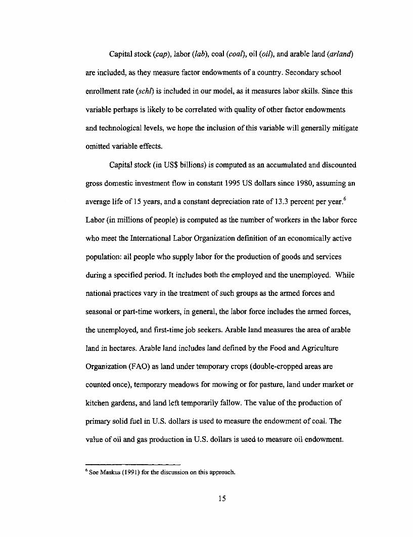
Capital stock (cap), labor (lab), coal (coal), oil (oil), and arable land (arland)

are included, as they measure factor endowments of a country. Secondary school

enrollment rate (schl) is included in our model, as it measures labor skills. Since this

variable perhaps is likely to be correlated with quality of other factor endowments

and technological levels, we hope the inclusion of this variable will generally mitigate

omitted variable effects.

Capital stock (in US$ billions) is computed as an accumulated and discounted

gross domestic investment flow in constant 1995 US dollars since 1980, assuming an

average life of 15 years, and a constant depreciation rate of 13.3 percent per year.6

Labor (in millions of people) is computed as the number of workers in the labor force

who meet the International Labor Organization definition of an economically active

population: all people who supply labor for the production of goods and services

during a specified period. It includes both the employed and the unemployed. While

national practices vary in the treatment of such groups as the armed forces and

seasonal or part-time workers, in general, the labor force includes the armed forces,

the unemployed, and first-time job seekers. Arable land measures the area of arable

land in hectares. Arable land includes land defined by the Food and Agriculture

Organization (FAO) as land under temporary crops (double-cropped areas are

counted once), temporary meadows for mowing or for pasture, land under market or

kitchen gardens, and land left temporarily fallow. The value of the production of

primary solid fuel in U.S. dollars is used to measure the endowment of coal. The

value of oil and gas production in U.S. dollars is used to measure oil endowment.

6 See Maskus (1991) for the discussion on this approach.

15

The variable schl follows the definition of the International Standard

Classification of Education on a net secondary school enrollment ratio. It is the ratio

(in percent) of the number of children at the official school age (as defined by the

national education system) who are enrolled in school, to the population of the

corresponding official school age. Secondary education completes the provision of

basic education that began at the primary level, and aims to lay the foundation for

lifelong learning and human development, by offering more subject- or skill-oriented

instruction, with more specialized teachers.

Data on capital, labor, and secondary school enrollment were obtained from

the World Development Indicators of the World Bank. Data on oil and gas production

(in millions of barrels), and coal (in millions of short tons) were obtained from the

U.S. Department of Energy (USDOE) database.

In our model, the state of legislation (leg) is constructed from the Dasgupta et

al. (2001) dataset, and has been used as the measure of an environmental standard. It

is measured by aggregating the scores on the scope of legislation enacted in the

manufacturing sector (see Table 1 for the total scores on legislation). Similarly, the

scores on the control mechanism for environmental enforcement (cm) are calculated

by aggregating the scores on the control mechanism for environmental enforcement

for the manufacturing sector.

As discussed earlier, the effect of legislation may differ according to the state

of the control mechanism for environmental enforcement. As modeled in Smarzynska

and Wei (2001), an inclusion of a product term between the legislation and a control

mechanism variable is intuitive. The product term allows a slope for the legislation

16

variable to vary across countries, particularly between developed and developing

countries.

In addition, unobserved differences between developed and developing

countries can be controlled by using a slope dummy for developed (or developing)

countries. We use a dummy variable for OECD membership, DOECD. How the state

of a control mechanism for environmental enforcement, and the stage of development

will affect the effectiveness of legislation can thus be tested by examining statistical

significance of 68 and /9, respectively. The total effect of the state of legislation can

be tested by investigating the statistical significance of /, + 3,B cm + 89g for the

OECD countries and 87 + / 8cm for the non-OECD countries. Details of this effect

will be explained later in Section 6.

Statistical independence between the explanatory variables is required for

reliable parameter estimates, but Table 4 indicates possible multi-collinearity in some

pairs of the variables. It is particularly problematic when key variables from which

policy implication is to be derived are correlated with other explanatory variables.

Notably, leg and cm are highly correlated, which will likely prevent deriving separate

policy implications of each variable, thus, instrumental variables are used for each of

these variables. Instrumental variables are chosen such that they are not correlated

with the other instrumental variables, and also with the instruments for that variable.

Data on these instruments are obtained from the Environmental Sustainability Index,

developed jointly by the World Economic Forum's Global Leaders for Tomorrow

Environment Task Force, the Yale Center for Environmental Law and Policy, and the

Columbia University Center for International Earth Science Information Network

17

(2001), except for the data on a country's total government expenditure, which is

obtained from the World Bank's World Development Indicators (1995-1998).

The instruments used for legislation are: (1) the number of memberships in

environmental intergovernmental organizations (eionum); (2) percentage of cites

reporting requirements met (cites); (3) levels of ratification under the Vienna

convention for the protection of the ozone layer (vienna); (4) Montreal protocol

multilateral fund protection (monfun); (5) the number of ISO 14001 certified

companies per GDP (isol.4); and (6) environmental strategies and action plans

(plans). The instruments used for the control mechanism variable are (1) members of

the International Union for Conservation of Nature and Natural Resources (IUCN)

(iucn), (2) government expenditure per capita (gov), and (3) the number of sectoral

EIA guidelines (eia).7 While the choice of these instrumental variables is based on

the logical linkage and causal relationship, we also chose them such that they were

not strongly correlated with other explanatory variables in Equation (1) and their

counterpart instrumental equation (see T'able 4).

The two instrumental equations are assumed to take a linear form:

legj, =ao + aleionumjB ++ a 2citesj1 + a3 viennajt

+ a4 monfun j, + a, isol 4 j,± + wj. (2)

cmj1 =Y + y,iucnj, + y 2 gov1 , + y 3 eiaj, + j (3)

A Non-Linear Two-Stage Least Squares (NL2SLS) method is used to estimate

equation (1) for the five pollution-intensive good exports. NL2SLS method is used

18

because a product term makes the model structure non-linear and also to account for

the presence of instrumental variables in the product term. Kelejian (1991) offers an

approach that estimates a system of non-linear equations. He suggests estimating first

the slope parameters equation by equation, then calculating the gradients of these

equations with respect to the slope parameters, and evaluating them at the estimated

values of these parameters. Then use these gradient vectors as instruments for the

dependent variables.

We have one non-linear equation and two instrumental equations. Thus, we

have three dependent (or endogenous) variables. Amemiya (1976) indicates that a

different set of gradients can be used for each equation. This allows us to have a

rather simple equation system. We use the original 6 and 3 instrumental variables for

leg and cm, respectively. We also use the explanatory variables in Equation (1) as

instruments for nex. This makes Equations (1), (2) and (3) unchanged. But it is

necessary to include an additional equation that has the product termn, leg cm, as the

instrumental variable. It is because this term is also a gradient, and consists of two

dependent (or endogenous) variables. We use all 9 of the instrumental variables for

leg and cm, and the product terrns that pair each of the 6 instrumental variables for leg

and each of the 3 instrumental variables for cm, as they logically follow. The

instrumental equations for leg, cm and the product term, are fitted in the first stage.

In the second stage, Equation (1) is estimated by replacing the corresponding

variables with these fitted values. In this stage, we corrected for heteroscedasticity in

7 While the use of these instrumental variables follow a logical order, a necessary assumption is made

that the instrumental variables are unchanged over time.

19

Equation (1) by weighting the observations by the square root of the OLS estimated

variances from the individual country.8

6. Results

The results are reported in Table 5. Capital is found to be significant for all of the five

industries with a negative effect for the Mining and Nonferrous Metals industries and

positive effect for the Pulp and Paper, Iron and Steel and Chemicals industries. Labor

is positive and significant for the Chemicals industry, but it is insignificant for the

Nonferrous Metal industry, and significantly negative for the Mining, Pulp and Paper

and Iron and Steel industries. The coefficient estimate for coal is found to be positive

and marginally significant for the Nonferrous Metals and Iron and Steel industries,

while it is significantly negative for the Metal Mining industry. The effect of coal in

the Pulp and Paper and Chemicals industries is insignificant. Arable land has a

significant effect in all of the industries, with varying signs across industries. Oil is

significant for the Mining and Chemicals industries, with a positive effect in the

Mining industry, and a negative effect in the Chemicals industry. Oil is insignificant

in the other three industries (Nonferrous Metals, Pulp and Paper, and Iron and Steel).

Labor skills, as measured by the variable school, appear to have a positive significant

relationship with net exports for all the industries, except for the Pulp and Paper

industries, where it is insignificant. Negative coefficient estimates for the factor

endowment variables, in some cases, are difficult to explain by real world

observations. It is perhaps due to the high correlation among these variables.

8 See Amemiya (1985) for the detail of this method.

20

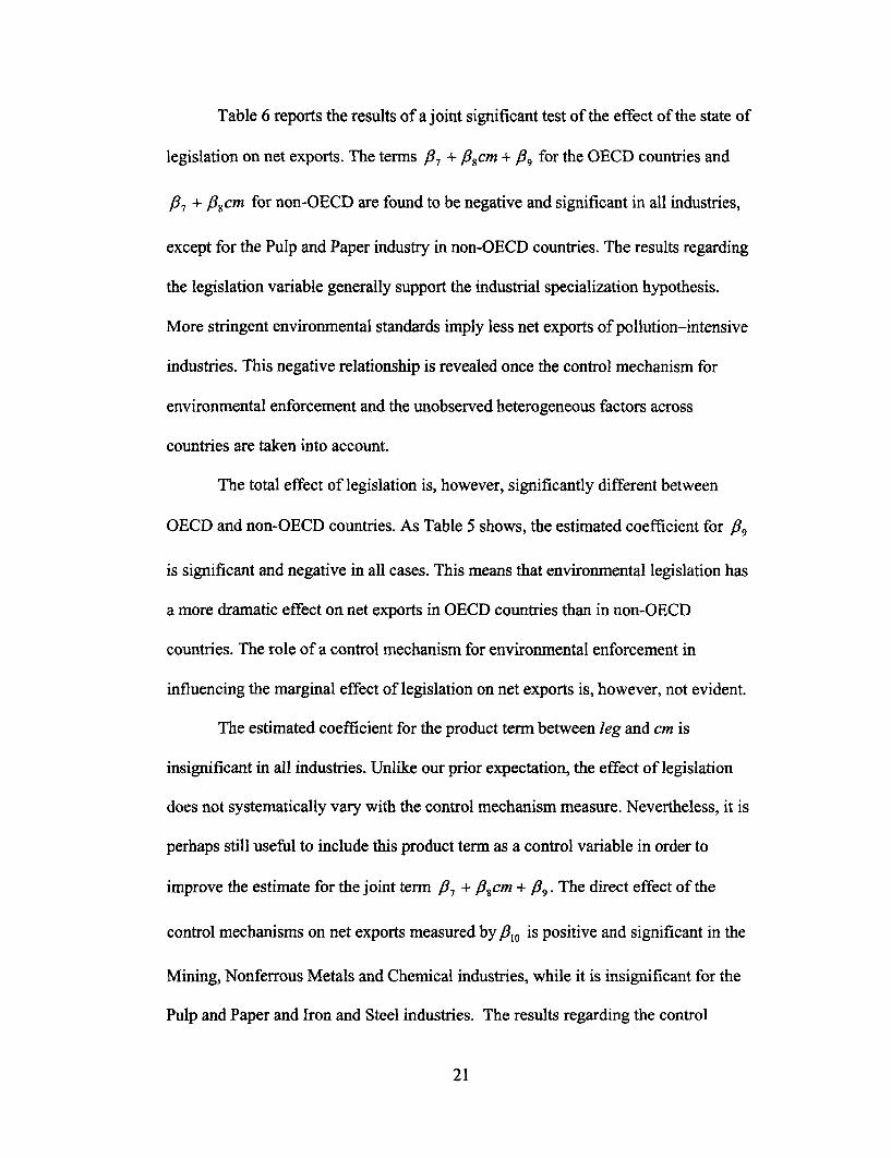
Table 6 reports the results of a joint significant test of the effect of the state of

legislation on net exports. The terms A7 + /38 cm + fig for the OECD countries and

67 + 48cm for non-OECD are found to be negative and significant in all industries,

except for the Pulp and Paper industry in non-OECD countries. The results regarding

the legislation variable generally support the industrial specialization hypothesis.

More stringent environmental standards imply less net exports of pollution-intensive

industries. This negative relationship is revealed once the control mechanism for

environmental enforcement and the unobserved heterogeneous factors across

countries are taken into account.

The total effect of legislation is, however, significantly different between

OECD and non-OECD countries. As Table 5 shows, the estimated coefficient for 8,3

is significant and negative in all cases. This means that environmental legislation has

a more dramatic effect on net exports in OECD countries than in non-OECD

countries. The role of a control mechanism for environmental enforcement in

influencing the marginal effect of legislation on net exports is, however, not evident.

The estimated coefficient for the product term between leg and cm is

insignificant in all industries. Unlike our prior expectation, the effect of legislation

does not systematically vary with the control mechanism measure. Nevertheless, it is

perhaps still useful to include this product term as a control variable in order to

improve the estimate for the joint term fl, + /8cm + /3g. The direct effect of the

control mechanisms on net exports measured by,8 10 is positive and significant in the

Mining, Nonferrous Metals and Chemical industries, while it is insignificant for the

Pulp and Paper and Iron and Steel industries. The results regarding the control

21

mechanism variable generally differ from the prior expectation. If the results are

considered to reflect the true underlying relationship, the insignificant sign on the

product term may reflect that the effectiveniess of legislation may be enhanced more

significantly by factors other than control mechanisms for environmental

enforcement. The positive sign on the single term may reflect the fact that improved

control mechanisms for environmental enforcement imply better compliance ability

of the country to the environmental standards of its exporting partners.

7. Conclusions and Policy Implications

What do these findings suggest in regard to trade policy and multilateral disciplines

on environmental protection? Our analysis suggests that environmental regulation can

affect export competition. The negative relationship between the stringency of

environmental standards and exports in the majority of industries examined may

imply a possible trade-off between two goals-trade expansion and encouraging

improvements in environmental standards. If developing countries do not place an

emphasis on environmental quality, they are reluctant to tighten environmental

standards. This could then result in a so-called "race-to-the-bottom" as with lack of

international coordination pollution may become more concentrated in the developing

countries.

If developed countries, instead, seek to harmonize environmental standards

globally at high levels, through trade agreements, then developing countries may

suffer from a greater loss in exports of the pollution-intensive products than a

developed country. For example, suppose that all of the countries in our sample

22

harmonize environmental standards at the most stringent level (Germany, Ireland, the

Netherlands, and Switzerland). Based on our estimated slope parameters, a non-

OECD country will, on average, reduce exports of the five pollution-intensive

products by US$ 2.6 million each year, or 0.37 percent of the average GNP of the

non-OECD countries in our study. This represents 11 percent of annual exports of

these products from the 24 studied countries. In contrast, an OECD country, on

average, will reduce annual exports by US$ 0.62 million, or 0.0 19 percent of the

average GNP of the OECD countries in our study. This is 2.5 percent of annual

exports of these products from the 24 studied countries.

This illustrates that global harmonization of environmental standards reduce

developing country exports of pollution-intensive goods more than exports from

developed countries. Our findings suggest tighten environmental standards in

developing countries gradually with transition periods could avoid rapid decline in

net exports of pollution-intensive products. It is also important to raise public

environmental awareness in developing countries so that the loss of export

competitiveness in these products are placed within the context of improved

environmental benefits.

The implications of our analysis are more complex, but remain relevant, for

questions of trans-boundary pollution that form the core agenda of the new WTO

negotiations. The results do indicate a relationship between standards and trade.

Developed countries are motivated to set a high global environmental standard in

multilateral environmental agreements, as they tend to benefit more from reductions

in trans-boundary pollution produced outside their borders. Some of the pollution

23

generated by the industries studies here do cross national borders. International

coordination to offset loss in export competitiveness shown here should be part of

discussion at the WTO. Moreover, the targeting principle that suggests that

addressing pollution emissions at the source through taxes and other direct domestic

policy instruments-rather than through trade sanctions or limits on imports of goods

by trading partners-remains the more rational policy prescription to suggest in this

area, rather than embedding new obligations in trade agreements at the WTO.

24

References

Amemiya, T. 1976. Estimation in Nonlinear Simultaneous Equation Models. Paperpresented at Institut National de La Statistique et Des Etudes Ecnomiques, Paris,March 10 and published in Malinvaued, E. (ed.), Cahiers Du SeminarireD'econometrie, no 19.

Amemiya, T. 1985. Advanced Econometrics. Cambridge: Harvard University Press.

Antweiler, W., B. Copeland, and S. Taylor. 1998. Is Free Trade Good for theEnvironment? Discussion paper # 98-11, Department of Economics,University of British Columbia, Canada.

Dasgupta, S., Mody, A., Roy, S., and D. Wheeler. 2001. Environmental Regulationand Development: A Cross-Country Empirical Analysis. Oxford DevelopmentStudies, Vol. 29(2):173-187.

Dean, J.M. 1992. Trade and the Environment, A Survey of the Literature in WorldBank Discussion Paper Series #159, 15-28. Washington, D.C.: The World Bank.

Duerksen, C.J. 1983. Environmental Regulation of Industrial Plant Siting.Washington, D.C.: The Conservation Foundation.

Environmental Sustainability Index. 2001. World Economic Forum, Yale Center forEnvironmental Law and Policy.http://www.ciesin.org/indicators/ESI/downloads.html#report.

EPA Office of Compliance Sector Notebook Project. 1995. Washington, D.C.:U.S. Environmental Protection Agency.

Friedman, J., D. Gerlowski, and J. Silberman. 1992. What Attracts ForeignMultinational Corporations? Evidence from Branch Plant Location in the UnitedStates. Journal of Regional Science 32: 403-418.

Gray, W. 1997. Manufacturing Plant Location: Does State Pollution RegulationMatter? National Bureau of Economic Research (NBER) Working Paper # 5880.Boston, Massachusetts: NBER.

25

Grossman, G.M. and A.B. Krueger. 1993. Environmental Impacts of a NorthAmerican Free Trade Agreement. In The Mexico-U.S. free trade agreement, ed.P.M. Garber. 13-56. Cambridge, Massachusetts and London: MIT Press.

Kalt, J.P. 1988. The Impact of Domestic Environmental Regulatory Policies on U.S.International Competitiveness. In International Competitiveness, A.M Spence andH.A. Hazard, eds. 221-262. Cambridge, Massachusetts: Ballinger.

Kelejian, H. 1971. Two-stage Least Squares and Econometric Systems Linear inParameters but Nonlinear in the Endogenous Variables, Journal of the AmericanStatistical Association. 66: 373-374.

Leamer, E.E. 1984. Sources of International Comparative Advantage: Theory andEvidence. Cambridge Massachusetts: MIT Press.

Leonard, H.J. 1988. Pollution and the Struggle for World Product. Cambridge,Massachusetts: Cambridge University Plress.

List, J.A. and C.Y. Co. 1999. The Effects of Environmental Regulations on ForeignDirect Investment. Journal of Environmental Economics and Management.40: 1-20.

Low, P. and A. Yeats. 1992. Do Dirt Industries Migrate? World Bank DiscussionPaper Series #159. 89-103. Washington, D.C.: The World Bank.

Levinson, A. 1996. Environmental Regulations and Manufacturers Location Choices,Evidence from the Census of Manufacturers. Journal of Public Economics 62:5-29.

Lucas, R.E.B., D. Wheeler, and H. Hettige. 1990. Economic Development,Environmental Regulation and the International Migration of Toxic IndustrialPollution. Paper presented at the Symposium on International Trade and theEnvironment, Washington D.C.

Mani, M., S. Pargal, and M. Huq. 1997. Does Environmental Regulation Matter?Determinants of the Location of New Manufacturing Plants in India. PolicyResearch Working Paper # 1718. Washington, D.C.: The World Bank.

Maskus, K.E. 1991. Comparing International Trade Data and Product and NationalCharacteristics Data for the Analysis of Trade Models. In International economictransactions. Issues in measurement and empirical research, P. Hooper and J.D.Richardson, eds. National Bureau of Economic Research Studies in Income andWealth. 55: 17-56. Chicago, Illinois and London: University of Chicago Press.

Nordstr6m, H. and S. Vaughan 1999. Trade and Environment. Geneva, Switzerland:World Trade Organization.

26

Pearson, C. 1987. Multinational Corporation, the Environment and Development.Washington, D.C.: World Resources Institute.

Smarzynska, B.and S. Wei. 2001. Pollution Havens and the Location of ForeignDirect investment: Dirty Secret or Popular Myth? June 10, 2001. Washington,D.C.: International Trade Team - Development Economics Research Group, TheWorld Bank. Mimeo.

Tobey, J.A. 1990. The Effects of Domestic Environmental Policies. Kyklos,43(2):191-209.

UNCED. 1990. Draft Format for National Reports. Geneva: United NationsConference on Environment and Development.

World Bank. 2000. Global Economic Prospects and the Developing Countries 2001.Washington, D.C.: The World Bank.

Xu, X. 1999. International Trade and Environmental Regulation: A DynamicPerspective. Huntington, New York: Nova Science Publishers, Inc.

Wheeler, D. 2000. Racing to the Bottom? Foreign Investment and Air Pollution inDeveloping Countries. Policy Research Working Paper #2524. Washington, D.C.:The World Bank.

27

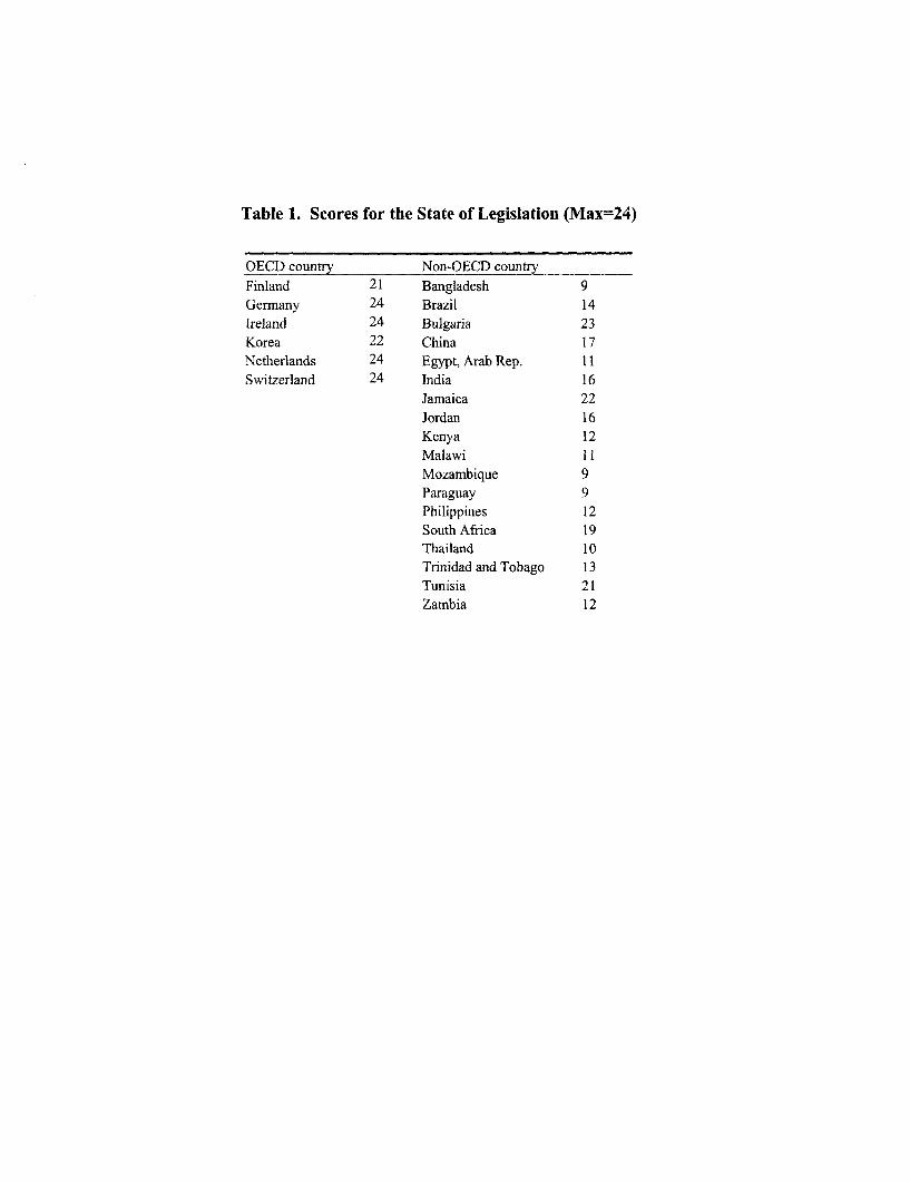
Table 1. Scores for the State of Legislation (Max=24)

OECD country Non-OECD countryFinland 21 Bangladesh 9Germany 24 Brazil 14Ireland 24 Bulgaria 23Korea 22 China 17Netherlands 24 Egypt, Arab Rep. 11Switzerland 24 India 16

Jamaica 22Jordan 16Kenya 12Malawi 11Mozambique 9Paraguay 9Philippines 12South Africa 19Thailand 10Trinidad and Tobago 13Tunisia 21Zambia 12

Table 2. Major Pollutants and Pollution Prevention Activities

Major chemicals contributing to Major pollution prevention activities Pollution abatementpollution costs as percentage of

total costs

Metal Mining Chlorine, Arsenic, Cadmium. Flotation, leaching, tailing, metal parts cleaning, blasting and 1.92-2.03crushing.

Nonferrous Metal Chlorine, Copper compounds, Zinc Process equipment modification, raw materials substitution or 2.05compounds, Lead compounds, and elimination,Sulfuric acid. solvent recycling, precious metals recovery.

Pulp and Paper Methanol, Hydrochloric acid, Sulfuric Extended delignification, enzyme treatment of pulp, chlorine 2.40acid, Chloroform. dioxide substitution, improved chipping and screening, improved

chemical controls and mixing.Iron and Steel Hydrochloric acid, Ammonia, Zinc Reducing cokemaking emissions, reducing wastewater volume. 2.38

compounds.Inorganic Chemical Hydrochloric acid, Chromium, Substitution of raw materials, improve reactor efficiencies and 2.89

Carbonyl Sulfide, Ammonia. catalyst, improve wastewater treatment and recycling.Plastics Trichloroethane, Acetone, Carbon Overall process to control for waste water, disposal and pellet 2.36

disulfide. release.Organic Chemical Sulfuric acid, Methanol and Overall process to control for catalysts, raw materials e.t.c. 1.53-2.89

tert-butyl alcohol.Source: U.S. EPA (1995) and Tobey (1990).

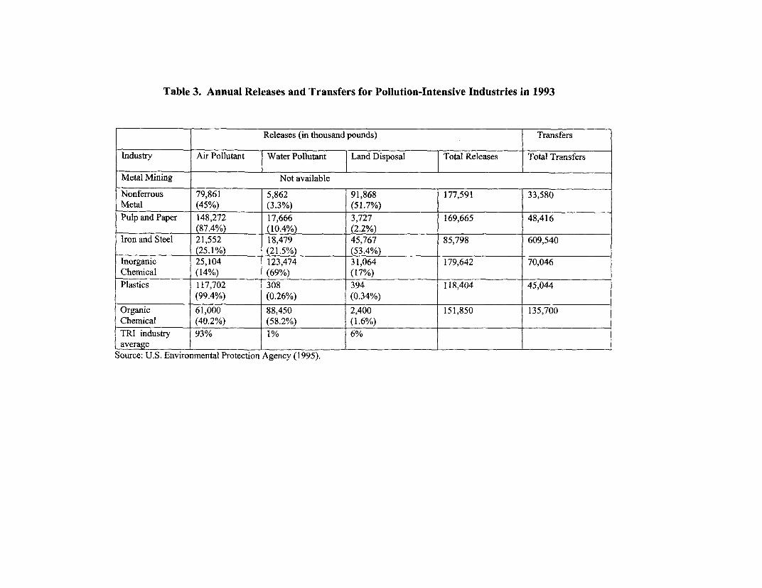
Table 3. Annual Releases and Transfers for Pollution-Intensive Industries in 1993

Releases (in thousand pounds) Transfers

Industry Air Pollutant Water Pollutant Land Disposal Total Releases Total Transfers

Metal Mining Not available

Nonferrous 79,861 5,862 91,868 177,591 33,580Metal (45%) (3.3%) (51.7%)

Pulp and Paper 148,272 17,666 3,727 169,665 48,416(87.4%) (10.4%) (2.2%)

Iron and Steel 21,552 18,479 45,767 85,798 609,540(25.1%) (21.5%) (53.4%)

Inorganic 25,104 123,474 31,064 179,642 70,046Chemical (14%) (69%) (17%) , _

Plastics 117,702 308 394 118,404 45,044(99.4%) (0.26%) (0.34%)

Organic 61,000 88,450 2,400 151,850 135,700Chemical (40.2%) (58.2%) (1.6%) __ _

TRI industry 93% 1% 6%average

Source: U.S. Environmental Protection Agency (1995).

Table 4. Correlation Coefficient Matrix

Explanatory variables Instrumentscap lab arland schl coal oil leg cm eionum cites vienna monfun isol4 plans iucn gov eia

cap 1.00lab 0.11 1.00arland 0.11 0.98 1.00schl 0.33 -0.17 -0.14 1.00coal 0.52 0.68 0.68 0.17 1.00oil 0.13 0.50 0.58 -0.02 0.29 1.00leg 0.36 -0.11 -0.09 0.76 0.19 -0.20 1.00cm 0.50 -0.13 -0.13 0.73 0.21 -0.20 0.86 1.00eionum 0.57 0.22 0.23 0.64 0.33 0.32 0.53 0.73 1.00cites 0.31 0.22 0.20 0.10 0.38 -0.22 0.18 0.24 0.21 1.00vienna 0.29 -0.37 -0.37 0.39 -0.23 0.03 0.41 0.30 0.32 -0.07 1.00monfun -0.06 -0.23 -0.20 0.27 -0.06 -0.08 0.39 0.25 0.00 -0.24 0.38 1.00isol4 0.02 -0.04 -0.03 0.06 -0.08 0.05 0.06 0.07 0.15 0.19 -0.04 -0.06 1.00plans -0.08 0.31 0.30 0.14 0.25 0.22 0.08 0.23 0.45 0.10 -0.14 -0.17 -0.22 1.00iucn -0.19 -0.37 -0.34 0.27 -0.25 -0.37 0.45 0.49 0.11 -0.03 0.16 0.18 0.04 0.23 1.00gov 0.50 -0,17 -0.17 0.59 0.08 -0.16 0.67 0.93 0.79 0.26 0.28 0.13 0.17 0.30 0.44 1.00eia 0.07 0.47 0.46 0.09 0.51 0.50 -0.07 0.09 0.43 0.06 -0.26 -0.07 0.35 0.48 -0.21 0.18 1.00

Table 5. Coefficient Estimates for 5 Pollution-Intensive Goods' Net Exports (Non-linear 2SLS)

Metal Mining NFMetals Pulp&Paper Iron&Steel Chemicals

Intercept -1004.63*** -1211.35*** -824.21 -795.73 -7296.56***

(170.68) (287.06) (724.05) (935.18) (1689.84)

Capital -0.39*** -0.12* 0.47* 1.48*** 2.96***

(0.07) (0.07) (0.25) (0.21) (0.46)Labor -29.78*** 0.75 -14.88*** -23.6*** 49.29***

(1.62) (1.34) (2.53) (4.79) (7.71)Coal -1.14*** 0.49* 0.60 2.53* 1.78

(0.42) (0.28) (0.65) (1.44) (2.22)Oil 1.76*** 0.09 -0.46 1.3 -3.28***

(0.26) (0.18) (0.33) (0.87) (0.83)Land 80.27*** -7.61** 33.61*** 51.39*** -137.15***

(3.95) (3.2) (6.62) (12.2) (17.46)

School 8.86*** 5.26*** -0.82 12.91*** 32.58***

___________ (1.7) (1.68) (1L52) (4.55) (7.59)

Legislation -87.08*** -31.48** 6.18 -104.65* -74.21*(9.04) (12.67) (15.86) (39.04) (42.00)

DOECD *Legislation -76.22*** -61.3*** -39.17* -72.34* -200.81***(7.47) (11.03) (20.72) (42.61) (64.83)

Legislation*Control Mechanism -0.02 -0.03 -0.26 -0.02 0.31

(0.13) (0.04) (0.25) (0.11) (0.29)Control Mechanism 51.42*** 37.87*** -24.26 37.12 165.77***

(5.13) (8.25) (19.85) (29.06) (41.75)

Time dummy for 1995 -77.78 -42.9 -26.17 -103.4 -0.31

(51.03) (31.93) (70.83) (94.3) (130.14)

Time dummy for 1996 -45.59 -25.00 -21.6 -61.00 -84.4(48.5) (36.75) (71.68) (117.08) (138.16)

Time dummy for 1997 -92.94* -39.26 -2.94 -7.76 -83.31

(51.08) (37.07) (71.9) (119.47) (140.64)

Time durnmy for 1998 -77.98 -37.29 35.22 -37.1 -198.25

(52.45) (38.02) (72.05) (132.81) (191.62)

Number of obs 77 93 111 97 97

Log-likelihood -500.65 -594.38 -804.41 -745.32 -790.85Note: Inside parentheses are standard errors. Notations "*", ""*"and "***" signify significance at the

10, 5 and I percent levels based on a two-tailed test, respectively.

Table 6. Joint Hypothesis Testing on the Effect of Legislation

___ M_ etal Mining NFMetals Pulp&Paper Iron&Steel Chemicals

OECD countries _ _ _

E(0 7+ 09+E(cm)* 38) -164.09 -93.93 -44.40 -177.81 -261.5

SE(,87+ 9+E(cm)* 8) 15.03 20.48 24.15 70.05 88.4Assym. t value -10.92 -4.59 -1.84 -2.54 -2.9Statistical significance 1/ 10/ 50/ 10/ 10/

Non-OECD countries_ __ _ _ _

E(07+E(cm)* 8) -87.87 -32.63 -5.23 -105.4 -60.7

SE(0l7+E(cm)* 0s) 11.85 12.12 10.13 38.3 47.1Assym. t value -7.4 -2.6 -0.5 -2.75 -1.2Statistical significance 10/ 10/ ns 10/ 100/

Note: "ns" means not significant.

Policy Research Working Paper Series

ContactTitle Author Date for paper

WPS2778 Technology and Firm Performance Gladys L6pez-Acevedo February 2002 M. Gellerin Mexico 85155

WPS2779 Technology and Skill Demand Gladys L6pez-Acevedo February 2002 M. Gellerin Mexico 85155

WPS2780 Determinants of Technology Adoption Gladys L6pez-Acevedo February 2002 M. Gellerin Mexico 85155

WPS2781 Maritime Transport Costs and Port Ximena Clark February 2002 E. KhineEfficiency David Dollar 37471

Alejandiro Micco

WPS2782 Global Capital Flows and Financing Ann E Harrison February 2002 K. LabrieConstraints Inessa Love 31001

Margaret S. McMillan

WPS2783 Ownership. Competition, and Geroge R. G. Clarke February 2002 P. Sintim-AboagyeCorruption: Bribe Takers versus Lixin Colin Xu 37644Bribe Payers

WPS2784 Financial and Legal Constraints to Thorsi:en Beck February 2002 A. YaptencoFirm Growth: Does Size Matter? Asli DiemirgOg-Kunt 38526

Vojislav Maksimovic

WPS2785 Improving Air Quality in Metropolitan The Mexico Air Quality February 2002 G. LageMexico City: An Economic Valuation Management Team 31099

WPS2786 The Composition of Foreign Direct Beata K. Smarzynska February 2002 P. FlewittInvestment and Protection of 32724Intellectual Property Rights: Evidencefrom Transition Economies

WPS2787 Do Farmers Choose to Be Inefficient? Donald F. Larson February 2002 P. KokilaEvidence from Bohol. Philippines Frank Plessmann 33716

WPS2788 Macroeconomic Adjustment and the Pierre-Richard Ag6nor February 2002 M. GosiengfiaoPoor: Analytical Issues and Cross- 33363Country Evidence

WPS2789 "Learning by Dining" Informal Somik V. Lall February 2002 Y. D'SouzaNetworks and Productivity in Sudeshna Ghosh 31449Mexican Industry

WPS2790 Estimating the Poverty Impacts of Jeffrey J. Reimer February 2002 P. FlewittTrade Liberalization 32724

Policy Research Working Paper Series

ContactTitle Author Date for paper

WPS2791 The Static and Dynamic Incidence of Dominique van de Walle February 2002 H. SladovichVietnam's Public Safety Net 37698

WPS2792 Determinants of Life Insurance Thorsten Beck February 2002 A. YaptencoConsumption across Countries Ian Webb 31823

WPS2793 Agricultural Markets and Risks: Panos Varangis February 2002 P. KokilaManagement of the Latter, Not the Donald Larson 33716Former Jock R. Anderson

WPS2794 Land Policies and Evolving Farm Zvi Lerman February 2002 M. FernandezStructures in Transition Countries Csaba Csaki 33766

Gershon Feder

WPS2795 Inequalities in Health in Developing Adam Wagstaff February 2002 H. SladovichCountries: Swimming against the Tide? 37698

WPS2796 Do Rural Infrastructure Investments Jocelyn A. Songco February 2002 H. SutrisnaBenefit the Poor? Evaluating Linkages: 88032A Global View, A Focus on Vietnam

WPS2797 Regional Integration and Development Maurice Schiff February 2002 P. Flewittin Small States 32724

WPS2798 Fever and Its Treatment among the Deon Filmer March 2002 H. SladovichMore or Less Poor in Sub-Saharan 37698Africa

WPS2799 The Impact of the Indonesian Lisa A. Cameron March 2002 P. SaderFinancial Crisis on Children: Data from 33902100 Villages Survey

WPS2800 Did Social Safety Net Scholarships Lisa A. Cameron March 2002 P. SaderReduce Drop-Out Rates during the 33902Indonesian Economic Crisis?

WPS2801 Policies to Promote Saving for Dimitri Vittas March 2002 P. InfanteRetirement: A Synthetic Overview 37642

WPS2802 Telecommunication Reforms, Access Antonio Estache March 2002 G. Chenet-SmithRegulation, and Internet Adoption Marco Manacorda 36370in Latin America Tommaso M. Valletti

WPS2803 Determinants of Agricultural Growth Yair Mundlak March 2002 P. Kokilain Indonesia, the Philippines, and Donald F. Larson 33716Thailand Rita Butzer

WPS2804 Liberalizing Trade in Agriculture: John S. Wilson March 2002 P. FlewittDeveloping Countries in Asia and the 32724Post-Doha Agenda

WPS2805 To Spray or Not to Spray? Pesticides, John S. Wilson March 2002 P. FlewittBanana Exports, and Food Safety Tsunehiro Otsuki 32724