discipline specific core course principles of

Graduate Course

Principles of Microeconomics II

CONTENTS

Lesson 1 : Monopoly

Lesson 2 : Some Applications of Monopoly

Lesson 3 : Monopolistic Competition

Lesson 4 : Oligopoly

Lesson 5 : Collusive Oligopoly

Lesson 6 : Consumer and Producer Theory in Action

Lesson 7 : Market Failure

Lesson 8 : Market for Factor Inputs Demand and Supply of Factors

Lesson 9 : Factor Pricing

Lesson 10 : International Trade

Lesson 11 : Terms of Trade, Free Trade and Protection

Editor :

Dr. Janmejoy Khuntia

SCHOOL OF OPEN LEARNING

University of Delhi

5, Cavalry Lane, Delhi-110007

1

LESSON 1

MONOPOLY

Perfect competition, as discussed earlier, represent an extreme market situation wherein

firms do not have any control over price determination. Besides this, free entry and exit

of firms, perfect knowledge about market conditions, perfect mobility of factors and no

government intervention make the competitive market efficient and welfare maximizing.

Perfect competition implies complete absence of monopoly power. But there could be

another extreme market situation wherein there is complete absence of competition which

is called monopoly.

1.1 LEARNING OBJECTIVES

After reading this lesson, you should be able to

(a) Understand the concept of monopoly

(b) Differentiate between different kinds of monopolies

(c) Analyze equilibrium of a monopolist firm

(d) Comprehend relationship between Price and quantity supplied.

(e) Explain and analyze the monopoly power

1.2 MEANING AND KINDS OF MONOPOLY

Monopoly has been derived from the combination of words ‘Mono + Polein’ where mono

means single and polein means to sell. So, monopoly can be defined as a market structure

where there is a single seller selling a product for which there is no close substitute

available and there are barriers to enter the market. Presence of a single firm shows that

there is no difference between a firm and an industry.

Features of Monopoly: Above definition of a monopoly reveals the following

characteristics of a monopolist:

1. Single Seller – In a monopoly there is just one seller of a product or service, there

being no difference between the firm and industry. The demand curve facing the

monopolist is thus the market demand curve. The monopolist thus fixes the price

and quantity where it maximizes its profits. However out of the two variables that

is price and quantity a monopolist can fix either of the variables. If it fixes the

price, quantity is determined by the market and if it fixes the quantity to be sold

then price is determined by the market.

2. No close Substitutes – For a monopolist to retain its position in the long run also

it is essential that the firm must be selling a unique product which cannot be

substituted by any other product or service.

3. No Entry – A monopolist usually earns supernormal profits in the long run as

there is no to entry of the new firms in the industry. So, the profit earned by the

monopolist is not wiped out as is the case in case of perfect competition where

presence of supernormal profits attracts new firms in the industry.

4. Goal of Profit Maximization – The goal of a monopolist firm is to maximize the

profits. How it maximizes the profits would be discussed under the next heading.

2

5. Absence of Supply Curve – In perfect competition there was a one to one

relation between price and quantity supplied. Such relation is absent in a case of a

monopoly as the quantity supplied is dependent upon the elasticity of the demand

curve and shape of the marginal cost. Thus, the same quantity can be supplied at

two different prices or two different quantities can be supplied at the same price

showing that there is no supply curve in monopoly.

Demand Curve under Monopoly

In case of a monopoly the firm itself is the industry which is therefore the price maker as

well as price taker unlike perfect competition where industry sets the price and all the

firms are just the price takers having no freedom of setting or changing the price. The

market demand curve in case of a monopoly is therefore the demand curve that the

monopolist firm faces whereas in perfect competition the demand curve of the firm is a

straight line parallel to X axis as given in diagram 1.

Diagram 1: Demand Curves under Perfect Competition and Monopoly

Total Revenue, Average Revenue and Marginal Revenue Under Monopoly

Take an imaginary revenue schedule of the monopolist as represented in Table 1.

Table 1

Price or Average

Revenue (AR)

Quantity Total Revenue

(TR)

Marginal Revenue

(MR)

100 1 100 –

90 2 180 80

80 3 240 60

70 4 280 40

60 5 300 20

3

50 6 300 0

40 7 280 – 20

30 8 240 – 40

20 9 180 – 60

10 10 100 – 80

This schedule shows the relation between price or average revenue and quantity in case of

monopoly. It shows that as price falls quantity demanded increases, ceteris paribus. Total

revenue thus first increases, reaches it’s maximum and then starts falling but it is always

nonzero and positive. Average Revenue (AR) and Marginal Revenue (MR) are falling.

AR remains higher than MR as quantity of output increases. MR is positive as long as

total revenue (TR) is increasing, when TR reached the maximum MR becomes zero and

when TR starts falling in absolute terms MR becomes negative. The shapes of the TR,

AR and MR curves are needed to be understood prior to deriving the equilibrium.

Diagram 2 is based on the values of TR, AR and MR given in Table 1.

Diagram 2: TR, AR and MR curves under Monopoly

Based on above discussion we can say that:

(1) Both AR and MR curves start from the same point on the price (vertical) axis.

(2) Both the curves are downward sloping.

(3) Slope of MR is twice the slope of AR.

4

Relation between MR, AR and Elasticity of demand in the below given results (Diagram

2):

4. If demand curve has unit elasticity i.e. Ed = 1, MR = 0

5. If demand curve is relatively elastic i.e. Ed > 1, MR = Positive

6. If demand curve is relatively inelastic i.e. Ed < 1, MR = Negative

Equilibrium under Monopoly

The objective of a monopolist is to maximize profits. There are two approaches to

maximize profits.

1) Total Approach

2) Marginal Approach

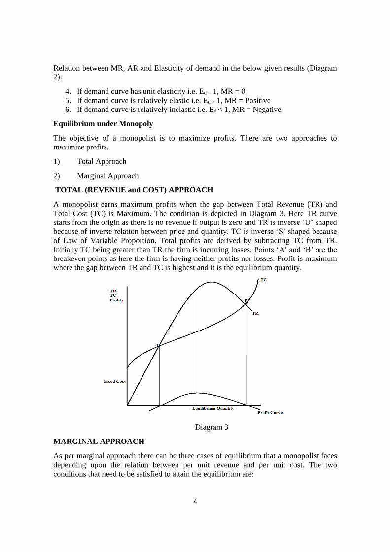
TOTAL (REVENUE and COST) APPROACH

A monopolist earns maximum profits when the gap between Total Revenue (TR) and

Total Cost (TC) is Maximum. The condition is depicted in Diagram 3. Here TR curve

starts from the origin as there is no revenue if output is zero and TR is inverse ‘U’ shaped

because of inverse relation between price and quantity. TC is inverse ‘S’ shaped because

of Law of Variable Proportion. Total profits are derived by subtracting TC from TR.

Initially TC being greater than TR the firm is incurring losses. Points ‘A’ and ‘B’ are the

breakeven points as here the firm is having neither profits nor losses. Profit is maximum

where the gap between TR and TC is highest and it is the equilibrium quantity.

Diagram 3

MARGINAL APPROACH

As per marginal approach there can be three cases of equilibrium that a monopolist faces

depending upon the relation between per unit revenue and per unit cost. The two

conditions that need to be satisfied to attain the equilibrium are:

5

(1) MR = MC

(2) MC cuts MR from below or Slope of MR < Slope of MC at the point of

equilibrium

Equilibrium of a monopolist can be derived under two time periods:

• Short Run – It’s a time period where there are certain costs that are fixed in nature

along with variable costs and entry or exit of the firms is not possible. Here a

monopolist can have supernormal profits; normal profits and can even incur

losses.

• Long run – It’s a time period where all costs become variable and entry or exit of

firms is also possible. Here a monopolist usually gets supernormal profits.

In the short run a monopolist may earn supernormal or abnormal profit or normal profit

or even incur loss depending on the position of short run average cost curve.

Case 1: Supernormal Profit

Diagram 4

Diagram 4 shows downward sloping Average revenue (AR) and Marginal revenue (MR)

curves. Short run average cost curve (SAC) and Short run marginal cost curves (SMC)

are also shown. Equilibrium is at point E where both the conditions of MR = MC and MC

cutting MR from below are being satisfied. Equilibrium quantity is OQ* that monopolist

would sell at a price of OP*. Total profits can thus be calculated as follows:

TP = TR – TC

= (Price * Quantity) – (Average Cost * Quantity)

= (OP*) * (OQ*) – (BQ*) * (OQ*) = OP*CQ* – OABQ* = AP*CB = Supernormal

Profits

6

Hence, condition for supernormal profits is that Price or AR > SAC.

Case 2: Normal Profit

In Diagram 5, equilibrium is at point E where both the conditions of MR = MC and MC


would sell at a price of OP*. See that in this case the SAC curve is tangent to AR curve at

point B implying that both AR and SAC are equal to BQ* = OP*. Total profits can thus

be calculated as follows:

TP = TR – TC


= (OP*) * (OQ*) – (BQ*) * (OQ*) = OP*BQ* – OP*BQ* = Zero = Normal Profits

Diagram 5

Hence, condition for Normal profits is given as Price or AR = SAC.

Case 3: Loss

Diagram 6

7

In Diagram 6, equilibrium is at point E where both the conditions of MR = MC and MC


would sell at a price of OP*. However, in this case the SAC curve is positioned above the

AR curve, thus implying that, SAC = CQ* which is more than AR = BQ* or OP*. Total

profits or losses can thus be calculated as follows:

TP = TR – TC


= (OP*) * (OQ*) – (CQ*) * (OQ*) = OP*BQ* – OACQ* = – P*ACB = Loss.

Hence, condition for loss is given as Price or AR < SAC

A monopolist can continue to operate despite having losses as there is a chance of earning

profits in the long run if the monopoly power is strong.

(2) Equilibrium in the Long Run

In the long run a monopolist can bring changes in the level of output by changing any

and/or all factors of production as there are no fixed factors in the long run. Here usually

a monopolist earns supernormal profits because of the barrier to entry of new firms. The

equilibrium is attained where long run marginal cost curve (LMC) is equal to marginal

revenue (MR) and LMC cuts MR from below. It is shown in Diagram 7. Figure shows

downward sloping Average revenue (AR) and Marginal revenue (MR) curves. Long run

average cost curve (LAC) and Long run marginal cost curves (LMC) are also shown.

Equilibrium is at point E where both the conditions of MR = LMC and LMC cutting MR

from below are being satisfied. Equilibrium quantity is OQ* that monopolist would sell at

a price of OP*. Total profits can thus be calculated as follows:

TP = TR – TC = (Price * Quantity) – (Average Cost * Quantity)

= (OP*) * (OQ*) – (BQ*) * (OQ*) = OP*CQ* – OABQ* = AP*CB = Supernormal

Profits

Diagram 7

8

1.3 ABSENCE OF SUPPLY CURVE IN MONOPOLY

In perfect competition the supply curve of a firm is the segment of marginal cost curve

above the minimum point of short run average variable cost curve. This is because of the

reason that the marginal revenue or the price curve is constant (parallel to x axis) and

hence it is only the marginal cost curve that is required for determining the quantity that

would be sold by a perfectly competitive firm at a particular price. Thus, it shows that

there is one to one relation between price and quantity supplied in case of perfect

competition as firm is only the price taker, price is set by the industry. This is however

not the case in monopoly. A monopolist firm has no supply curve as there is no one to

one relation between price and quantity supplied due to the fact that here demand curve is

not constant but is downward sloping. So, the quantity supplied at different prices depend

upon the shape of the demand curve (elasticity) and marginal cost curve as equilibrium is

obtained by the intersection of marginal revenue and marginal cost curve. It can be shown

by shifting the demand curves that two different quantities can be supplied at the same

price and the same quantity can be supplied at two different prices depending upon the

elasticity of the demand curve.

Case 1: Same quantity being supplied at two different prices – It is shown in Diagram

8. Here initially demand curve is shown by AR and corresponding marginal curve is MR.

Equilibrium is where AR and MR intersect, and it is obtained at point E where the

monopolist is selling OQ* units of commodity at a price of OP per unit. Now if the

demand curve shifts to AR1 with corresponding marginal revenue curve being MR1, the

new equilibrium is at the same point ‘E’ where monopolist is selling the same number of

units that is OQ* but at a reduced price of OP1 as the new demand curve is relatively

more elastic. Thus, it shows how change in the elasticity can force the monopolist to sell

the same quantity at different prices.

Diagram 8

9

Case 2: Two different quantities can be sold at same price – See Diagram 9 where the

initial demand curve is AR and corresponding marginal revenue curve is MR.

Equilibrium is at a point where MR and MC intersect that is point E showing that

monopolist is selling OQ units of commodity at a price of OP* per unit. Now if the

demand curve shifts to AR1 with corresponding marginal revenue curve being MR1, then

equilibrium shifts to E1 where monopolist is selling a higher quantity but at the same

price of OP*. Thus, it shows how monopolist cannot obtain any one to one relation

between price and quantity supplied as here the demand curve is downward sloping and

its elasticity and shape of marginal cost curve both have an impact on the equilibrium.

Diagram 9

Degree of Monopoly Power

Monopoly is a condition with only one seller having no close substitutes giving it the

freedom to set the price, however such pure monopoly rarely exist and what we have is

the situation where several firms compete with each other. In perfect competition each

firm earned only normal profits in the long run as if there is any supernormal profit in the

short run, new firms enter the market till all the excess profit is wiped out and all firms

set their equilibrium quantity at the point where marginal revenue is equal to marginal

cost. As in perfect competition price is constant thus price is equal to marginal revenue

and hence equilibrium is:

Price = MR = MC

But in case of monopoly demand curve is downward sloping therefore P > MR and

equilibrium condition being MR = MC, we get a difference between price and MC as P >

MC. This gap between price and MC shows the extent of monopoly power that a firm

possess.

Abba Lerner an economist gave an index in 1934 to measure this monopoly power and it

is called Lerner’s Index of Monopoly Power.

10

L = (P–MC) / P = – 1/ Ed where 0 ≤ L < 1

The more is the elasticity of the demand curve the lesser is the monopoly power and the

lesser is the elasticity of the demand curve the more is the monopoly power.

For perfect competition as P = MC, thus L = 0, there being no monopoly power.

The closer the value of L to 1, the higher is the monopoly power.

1.4 LEARNING OUTCOME

Monopoly is a market structure characterized by a single seller where the firm itself is the

industry. Monopolist firm thus faces a demand curve that is downward sloping and equal

to the market demand curve giving it the freedom to determine its equilibrium. This

however does not mean that the monopolist can charge any price and sell any quantity

that it desires. Out of the two variables (price and quantity) it can set only one and the

other is given by the market depending upon the shape of the demand and cost curves.

Equilibrium is where the marginal revenue and marginal cost curves intersect as if

monopolist sells an output less than this then marginal revenue being greater than

marginal cost it is losing profits and if it sets a quantity more than this then MR being less

than MC, monopolist is incurring losses thus the equilibrium is where MR becomes equal

to MC as this is the situation where profits are maximum. Unlike perfect competition

there is no supply curve of a monopolist firm, the reason being that there is no one to one

relation between price and quantity supplied. A monopolist can sell two different

quantities at the same price or same quantity at two different prices depending upon the

elasticity of the demand curves.

1.5 SELF ASSESSMENT QUESTIONS

Check your progress

Exercise 1: True and False

(a) In case of perfect competition there is no monopoly power.

(b) Firms can easily enter in a monopoly market structure.

(c) A monopoly firm always earns supernormal profits even in the short run.

(d) A monopolist can determine the price at which it sells the commodity as well as

the number of units it wants to sell.

(e) The objective of a monopolist is to maximize profits.

(f) The higher is the elasticity of demand curve the more is the monopoly power

(g) There is no supply curve in case of monopoly

Ans. 1(T), 2(F), 3(F), 4(F), 5(T), 6(F), 7(T)

Exercise 2: Fill in the Blanks

(a) Lerner’s Index is a tool to measure ……………….

(b) In case of perfect competition, the gap between price and marginal cost is

……………….

(c) A monopolist firm is the price ……………….

(d) There is ………………. of supply curve in case of monopoly

11

Ans 1. Monopoly Power 2. Zero 3. Maker as well as taker 4. Absence

Exercise 3: Questions

1. Using shifting demand curves show that there is no supply curve in case of

monopoly.

2. Explain the concept of Monopoly Power.

3. How does a monopolist firm reach its equilibrium in the short run?

4. Explain the relation between Average revenue, Marginal revenue and Elasticity of

demand.

Mathematical Proof (Optional)

1. Relation between Total Revenue (TR), Average Revenue (AR) and Marginal

Revenue (MR) under Monopoly

Let demand function of a monopolist is given by

P = a – bQ ……………………………………… (1)

Where P = Price, Q = Quantity, a = intercept and b = slope of the demand curve.

Now Total Revenue (TR) = P*Q, substituting Equation 1 in TR, we get:

TR = (a – bQ) * Q = aQ – bQ2

AR = TR / Q = (aQ – bQ2)/Q = a – bQ = Price ……………………………… (2)

MR = ∂TR/∂Q = ∂ (aQ – bQ2)/ /∂Q = a – 2bQ ……………………………… (3)

Comparing AR and MR i.e. equation (2) and (3) we get the following results:

AR = a – bQ

MR = a – 2bQ

a. Intercept of both AR and MR is same = a, so both the curves start from the same

point on the Y axis.

b. Both have a negative sign in between showing that both the curves are downward

sloping.

c. Slope of AR is ‘b’ and MR is ‘2b’, so slope of MR is twice the slope of AR.

2. Relation between AR, MR and Elasticity of Demand in case of a Monopoly

Total Revenue, TR = Price *Quantity = P*Q

Average Revenue, AR = TR/Q = P*Q)/Q = P

12

Marginal Revenue, MR = ΔTR/ΔQ = Δ (P*Q)/ΔQ = P (ΔQ/ ΔQ) + Q (ΔP/ ΔQ)

MR = P + Q (ΔP/ ΔQ)

Multiplying and dividing above by P we get following

MR = P + Q/P (ΔP/ ΔQ)*P . . . . . . . . . . . . . . . . . . . . . . . . . .(1)

Also, Ed = , (– ) 1/ Ed =

Substituting the value of Ed in Equation (1) we get

MR = P + P*[(– ) 1/ Ed], MR = P [1 – 1/ Ed ], MR = AR [1 – 1/ Ed ]

Above result shows relation between MR, AR and Elasticity of demand in the below

given results (Figure 1):

(a) If demand curve has unit elasticity i.e. Ed = 1, MR = 0

(b) If demand curve is relatively elastic i.e. Ed > 1, MR = Positive

(c) If demand curve is relatively inelastic i.e. Ed < 1, MR = Negative

3. Equilibrium Conditions

The objective of a monopolist is to earn profits and profits are maximized when the

following conditions are satisfied:

Total Profit (TP) = Total Revenue (TR) – Total Cost (TC)

To maximize profits the gap between total revenue and total cost should be maximized

i.e. first differentiation is equated to zero

∂TP/ ∂Q = ∂TR/∂Q – ∂TC/∂Q = 0

= MR – MC = 0,

MR = MC ………………………………1st order

condition

∂2TP/ ∂Q2 = ∂2TR/∂Q2 – ∂2TC/∂Q2 < 0

Slope of MR < Slope of MC ………………………………2nd order

condition

4. Rule of Thumb Pricing for Monopoly Power

As shown above the equilibrium of a monopolist is at a point where marginal revenue and

marginal cost curves intersect but it is not always feasible for the monopolist to trace the

marginal revenue and marginal cost curves for all the levels of output. Because of limited

knowledge it is preferable to use a rule of thumb for pricing as derived below.

13

MR = ∆TR/∆Q = ∆(P*Q)/ ∆Q. Using Product rule, we get:

MR = P + Q(∆P/∆Q). Multiplying and dividing the second part by P we get:

MR = P + (Q/P) (∆P/∆Q) * P ………………………… (1)

Ed = (∆Q/∆P) * (P/Q) or 1/ Ed = (Q/P) (∆P/∆Q) substituting this in Equation (1)

MR = P + (1/ Ed ) * P, MR = P (1 + 1/ Ed ) ………………………… (2)

Equilibrium condition is that MR = MC, substituting this in Equation (2)

MC = P (1 + 1/ Ed ) or P = MC / (1 + 1/ Ed ) or (P – MC)/P = – 1/ Ed

This is the rule of thumb for pricing. From this we can also move to the concept of

Monopoly Power.

14

LESSON 2

SOME APPLICATIONS OF MONOPOLY



a) Understand the concept of integration of firms.

b) Differentiate between perfect competition and monopoly.

c) Analyze different types of price discrimination.

d) Understand the concept of deadweight loss.

2.2 INTRODUCTION

A monopolist derives its monopoly power because of barriers to entry that prohibits new

firms to enter the market as if the barriers are not there then monopoly situation cannot

exist for long. The barriers can be natural barriers (raw material availability), economic

barriers (economies of scale, cost advantage or technological superiority) or legal barriers

(patents, copyrights, trademarks). Depending upon the monopoly power that a firm

possesses, monopolist can even go for price discrimination where it charges different

prices from different consumers for the same product. A pure monopoly situation can

reduce the consumer surplus (benefit of the society) to a great extent and hence it is

usually undesirable unless it is controlled by the state for welfare of the society at large or

it’s a natural monopoly (where it is more efficient to let it serve the entire market rather

than to have several firms). This chapter thus discusses about the difference between

perfect competition and monopoly, the costs that society has to bear because of monopoly

and various types of price discrimination that a monopolist can exercise.

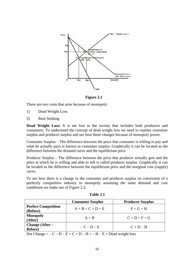
2.3 SOCIAL COSTS / ALLOCATIVE INEFFICIENCY OF MONOPOLY

In case of perfect competition, a firm sells a product at a point where Price (P) is equal to

marginal cost (MC). There being no cost to the society. A monopolist however sells at a

price that is greater than its marginal cost as is shown in Figure 2.1. Demand curve of a

perfectly competitive industry is downward sloping and supply curve obtained from

summation of the marginal cost curves is upward sloping. Equilibrium of the industry is

where demand is equal to supply, it gives OQpc quantity at OPpc price. If it would have

been a monopoly then equilibrium would be at a point where marginal revenue and

marginal cost is equal which is given by point A in the Figure 2.1, monopolist is selling

OQm quantity at a price of OPm. It can be seen that a monopolist sells lesser quantity as

compared to perfect competition and that too at a higher price. This leads to the cost that

society has to bear and termed as allocative inefficiency of monopoly market.

15

Figure 2.1

There are two costs that arise because of monopoly:

1) Dead Weight Loss

2) Rent Seeking

Dead Weight Loss: It is net loss to the society that includes both producers and

consumers. To understand the concept of dead weight loss we need to explain consumer

surplus and producer surplus and see how these changes because of monopoly power.

Consumer Surplus – The difference between the price that consumer is willing to pay and

what he actually pays is known as consumer surplus. Graphically it can be located as the

difference between the demand curve and the equilibrium price

Producer Surplus – The difference between the price that producer actually gets and the

price at which he is willing and able to sell is called producer surplus. Graphically it can

be located as the difference between the equilibrium price and the marginal cost (supply)

curve.

To see how there is a change in the consumer and producer surplus on conversion of a

perfectly competitive industry to monopoly assuming the same demand and cost

conditions we make use of Figure 2.2:

Table 2.1

Consumer Surplus Producer Surplus

Perfect Competition

(Before) A + B + C + D + E F + G + H

Monopoly

(After) A + B C + D + F + G

Change (After –

Before) – C – D – E C + D – H

Net Change = – C – D – E + C + D – H = – H – E = Dead weight loss

16

Figure 2.2

Initially we assume that there is perfect competition in the market. Here demand curve

AR and supply curve are given by Mc, equilibrium is where demand and supply curve

intersect which is given by Epc. Equilibrium quantity is Qpc and price is Ppc. Here the

consumer surplus and producer surplus are given in the table below. Now if all the firms

under perfectly competitive industry are undertaken by a monopolist assuming that

demand and cost conditions remain same, the equilibrium is obtained by intersection of

MR and MC which is at Em giving equilibrium quantity as Qm and price as Pm. It can be

seen that Monopolist is selling a lesser quantity and that too at a higher price. The new

consumer surplus and producer surplus is shown in the Table 2.1. To find out whether

consumers or producers are at loss or gain we calculate the change in consumer and

producer surplus. It is seen that consumer surplus has reduced by C + D + E, the

reduction of C + D being because of a higher price that consumers now have to pay while

reduction in E is because of reduction in the quantity as now few consumers have to do

without the commodity. Producer surplus on the other hand has increased by C + D but

reduced by H. The increase of C + D is because of higher price that producers get now; it

is actually just a transfer from consumers to producers (a zero sum game) and loss in H is

because of reduction in quantity that producers sell now. To find out whether society as a

whole is at gain or loss, we add the change in consumer and producer surplus and find out

that society at large is at a loss of H+E, this being the dead weight loss or cost to the

society because of monopoly.

2.4 COMPARISON OF PERFECT COMPETITION WITH MONOPOLY

1. Number of Sellers: Pure competition has many buyers and sellers whereas there is

just one seller in the monopoly.

2. Substitute Products: In Pure competition all firms sell identical (homogeneous)

products unlike monopoly where there are no close substitutes available.

3. Entry and Exit of Firms: Pure competition provides free entry and exit to the firms

though it is possible only in the long run while monopoly prevents entry of any

new firm to the industry.

17

4. Profits in the Long run: In perfect competition firms earn normal profits in the

long run while monopolist usually has supernormal profits because of barriers to

entry and exit.

5. Demand curve of the firm: Perfectly competitive firm has no control over the

price as it is the industry which fixes the price, the demand curve therefore is a

straight line parallel to X axis at the price given by the industry whereas

monopoly having just firm there is no difference between the firm and the

industry and market demand curve which is downward sloping is the demand

curve of the firm itself.

6. Social cost: A perfectly competitive industry sets its equilibrium at a point where

demand and supply are equal; hence there is no cost to the society. Monopolist

sets a price according to MR = MC where P > MC which brings cost to the

society.

7. Price Discrimination: A perfectly competitive industry cannot discriminate on the

basis of price whereas a monopolist can follow price discrimination.

8. Supply curve of the firm: A perfectly competitive firm has one to one relation

between price and quantity supplied which is shown by the supply curve which is

the segment of marginal cost over and above the minimum point of short run

average variable cost curve. However, there is no supply curve in case of

monopoly as same quantity can be sold at two different prices or two different

quantities can be sold at the same price depending upon the shape of demand

curve and marginal cost curve.

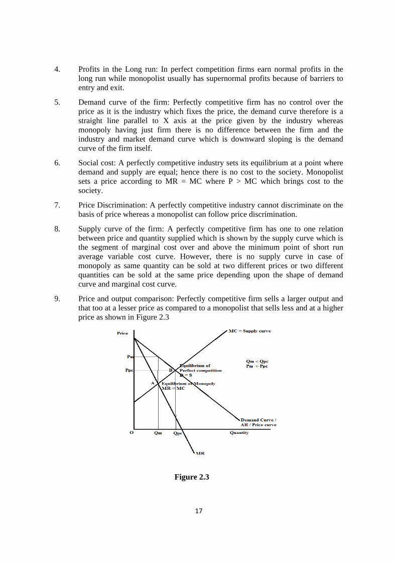
9. Price and output comparison: Perfectly competitive firm sells a larger output and

that too at a lesser price as compared to a monopolist that sells less and at a higher

price as shown in Figure 2.3

Figure 2.3

18

2.5 PRICE DISCRIMINATION

Price discrimination refers to charging different price from different consumers for the

same product. This is done by the monopolist to capture the consumer surplus that is

there with the consumers as is shown in Figure 2.4.

Figure 2.4

A single price monopolist would maximize its profits by setting the equilibrium where

MR=MC such that it sells OQm quantity at a price of OPm. Here the consumer surplus is

APmB. Now if the monopolist wants to earn even higher profits then it can go for price

discrimination such that it can charge different prices from different consumers like it can

charge higher price P1 from consumers who are willing to pay more and charge lower

price P2 and P3 from the consumers who cannot afford Pm. This way the monopolist can

earn even higher profits.

Pigou has described three degrees of price discrimination on the basis of how much

consumer surplus the monopolist can take away from the consumers.

1. First Degree Price Discrimination

2. Second Degree Price Discrimination

3. Third Degree Price Discrimination

First Degree Price Discrimination: There are two types of first-degree price

discrimination:

Case 1: The monopolist charges each consumer the maximum price that he is willing to

give – known as the reservation price thereby taking away all the consumer surplus of the

consumers. The demand curve here itself becomes the marginal revenue curve. Impact of

first-degree price discrimination is shown in Figure 2.5:

19

Figure 2.5

A single price monopolist charges OPm and sells OQm units of the commodity by

equating marginal revenue with the marginal cost. The consumer surplus here is shown

by the area APmB. Now if the monopolist goes for price discrimination then he would

charge the maximum price that a consumer is willing to give which is shown by the

demand curve. Thus, here MR curve becomes irrelevant as demand curve itself is the MR

curve for the discriminating monopolist. The consumer surplus is reduced to zero as

whatever price the consumer is willing to give the same is charged by the monopolist.

This is highest form of discrimination as nothing is left for the consumers as surplus. To

see how the monopolist is benefited by the price discrimination we calculate incremental

(variable) profits before and after the discrimination. Variable profits are calculated as the

difference between Marginal revenue and marginal cost as it is the incremental profit and

not the total profits.

Incremental profit before price discrimination is shown by the area of triangle ACEm

Incremental profit after price discrimination is shown by the area of triangle ACEpd

Thus, increase in the incremental profit = ACEpd – ACEm = Area of triangle AEmEpd. It is

shown by the shaded area in the Figure above.

However, there is a limitation of perfect first-degree price discrimination that is it is very

difficult if not impossible to find out the reservation price for each and every consumer.

This type of price discrimination is thus not found in real life, what we have is imperfect

first-degree price discrimination.

Case 2: In case 1 as discussed above, the monopolist charges different price from each

consumer depending on how much he is willing to pay. There is an alternative method as

well. The monopolist can also charge a few different prices based on the reservation

prices of different groups of consumers. So here there are certain ranges for different

consumers which a monopolist can still identify. For example, a doctor can charge

different fees depending upon the locality he is operating in. it is being explained in

Figure 2.6.

20

Figure 2.6

A single price monopolist would have sold OQ* units and charged a single price of OP3

from all the consumers. But in case of imperfect first-degree price discrimination,

monopolist sets 5 different prices that is P1, P2, P3, P4 and P5 which is being charged from

different consumers on the basis of the price that they are willing to pay. This type of

discrimination is called imperfect as there is still consumer surplus left with the

consumers unlike perfect first-degree discrimination. The price is set by identifying what

the marginal (last) consumer of that particular group is willing to pay. There can be

various price bands and monopoly equilibrium price can be one of them.

Second Degree Price Discrimination: A form of price discrimination where different

prices are charged from consumers on the basis of quantity being purchased. Thus, more

are the units purchased lesser is the price. Block pricing is also an example of second-

degree price discrimination where prices are different for different blocks (Figure 2.7).

With a single price to be followed a monopolist would set its output at OQm at a price of

OPm. However, with price discrimination on the basis of quantity being purchased by the

consumers there are three sets of prices that is P1, Pm and P2 for Q1, Qm and Q2 quantities

respectively. Here cost curves are not U shaped but downward sloping as it’s the case of a

natural monopoly. Thus, the last block is at a point where demand is equal to average cost

and not where demand is equal to marginal cost as at the latter point firm would be

incurring losses. Here also consumers are left with consumer surplus and all of it is not

taken away by the monopolist as price that the consumers have to pay is less than what

they are willing to pay which is shown by the demand curve.

21

Figure 2.7

Third Degree Price Discrimination: A discrimination that charges different prices from

different subgroups of the market for the same product with different elasticities thereby

charging a higher price in the subgroup that lower elasticity and lower price in the

subgroup having higher elasticity. It is the most common type of price discrimination. For

the firm to successfully follow third degree price discrimination following conditions

should be satisfied:

1. Firm is a monopolist.

2. The whole market is divided into sub-markets/subgroups. Let us assume that there

are two sub-markets/sub-groups.

3. Price elasticity of demand is different in the different sub-markets.

4. Sub-markets should be kept separate that is it should not be possible for the

consumers to shift themselves from one submarket to the other.

5. It should not be possible to transfer goods from one sub-market to other otherwise

arbitrage opportunities would eliminate the price differential thereby making price

discrimination infeasible.

Third degree price discrimination is explained with Figure 2.8 wherein the total market of

the monopolist is divided into two sub-markets. In sub-market 1 as shown in Panel 1 of

the figure 2.8, AR1 is the demand curve which is inelastic and hence it is steeper showing

that this sub-market is not that responsive towards prices. MR1 is the corresponding

marginal revenue curve. In sub-market 2 as shown in Panel 2 of the same figure, AR2 is

the demand curve that has greater price elasticity and is therefore flatter showing higher

responsiveness of the group towards price changes. MR2 is the corresponding marginal

revenue curve. The demand curves for the total market of the monopolist are derived by

adding up the demand curves of these two sub-markets. Panel 3 of the figure shows the

total AR and MR curves as AR1+2 and MR1+2 respectively where AR1+2 = AR1 + AR2 and

MR1+2 = MR1 +MR2.

22

Determining Equilibrium Condition

The condition for equilibrium is given as

1. MR1+2 = MR1 = MR2 = MC and

2. MC cuts MR1+2 from below.

Total Profits (Π) of the monopolist =

Total Revenue from first sub-market + Total Revenue from second sub-market – Total

cost

Π = TR1 + TR2 – TC

As per the marginal conditions stated above, first determine the equilibrium point at E0

where MR1+2 = MC as shown in Panel 3 of the figure 2.8. The rate of total quantity to be

produced by the monopolist is given as Q0 which corresponds to point E0. The price for

this rate of output should have been P0 as per standard practice of price setting by a

monopolist which is done on the AR1+2 curve. However, under price discrimination, the

monopolist does not charge P0 price nor sells Q0 quantity. Instead the monopolist divides

the total market quantity in two sub-markets by following the condition MR1+2 = MR1 =

MR2 = MC. Diagrammatically, this is done by drawing a horizontal line through the point

E0 such that the said line cuts MR1 at point E1 in sub-market 1 and MR2 at point E2 in

sub-market 2. Accordingly, in sub-market 1, rate of quantity corresponding to equilibrium

point E1 will be Q1 and price on its inelastic AR1 curve will be set at P1. Similarly, in sub-

market 2, rate of quantity corresponding to equilibrium point E2 will be Q2 and price on

its relatively elastic AR2 curve will be set at P2. See that Q0 = Q1 + Q2. It can also be

verified that P1 and P2 are not equal; rather P1 > P2 showing that a relatively elastic

demand curve commands a lower price as compared to relatively inelastic one. So, for the

same good the monopolist is charging two different prices in two different sub-markets

which conforms to price discrimination which is mainly made possible due to different

elasticities of demand in these two sub-markets.

Determining Relative Prices

In Chapter 1 we proved a relation between Average Revenue (AR), Marginal Revenue

(MR) and Elasticity of demand as:

MR = P (1 + 1/ Ed)

Using above equation for the two subgroups with different marginal revenue curves and

different elasticities we get:

MR1 = P1 (1 + 1/ Ed1) ………………………………. (1)

MR2 = P2 (1 + 1/ Ed2) ……………………………….(2)

In the equilibrium MR1 = MR2, thus equating equations (1) and (2) we get:

23

MR1 = MR2

P1 (1 + 1/ Ed1) = P2 (1 + 1/ Ed2 )

P1/ P2 = (1 + 1/ Ed2)/ (1 + 1/ Ed1) ………………………. (3)

From Equation (3) there can be two cases:

(a) If Ed1 = Ed2, then P1 = P2

(b) │Ed1 │ < │Ed2│, P1 > P2

Figure 2.8

2.6 NATURAL MONOPOLY

Natural Monopoly occurs in case of Public utilities like Electricity, water supply,

telephone services etc. where initial cost of the Plant remains higher but after that cost

start falling as well as output increases. That’s why under Natural Monopoly Average

Cost & Marginal Cost Curves are downward sloping & MC is always lower (below)

Average Cost. When there are no regulation impose on Natural Monopoly then they will

Produce qm quantity & sell at Pm price. But if Natural Monopoly is regulated then the

firm’s Price go down to the competitive market level Pc & quantity increases by qc. At

the Price of Pc firm would not cover average cost & firm will shut down or go out from

business. So, the Ideal option is to set the price Pn where AC, & AR intersect each other.

Here firms are not getting anormal monopoly profit but will produce large quantity of

output qn & without driving the firm out of business.

24

Figure 2.9

2.7 ANTITRUST LAWS

Antitrust Laws reduce market power & promote competition in market. As we

know that monopoly power, create social cost due to inefficient allocation of resources.

Antitrust laws vary from nation to nation. But the action of this laws is generally to

promote competitiveness in business world & restrict Monopoly Power & give (provide)

protection to the consumers. Antitrust Law prohibit those actions which create monopoly

or restrict competition.

Sherman Act, passed in 1890 prohibits contracts, combinations, or conspiracies in

restraint of trade.

The Clayton Act (1914) prohibits mergers & acquisitions which create monopoly power.

The antitrust laws also limit possible anticompetitive behavior of the firm.

Federal Trade commission Act (1914, amended in1938, 1973, 1995) is supplements the

Sherman & clayton acts by increasing competition & Put restrictions on unfair trade

practices, & anti competitive practices such as fraudulent advertising and labeling,

agreements with retailers to exclude competing brands, and so on. Because these

prohibitions are interpreted and enforced in administrative proceedings before the FTC,

the act provides broad powers that reach further than those of other antitrust laws.


Monopoly is a market structure characterized by a single seller possessing monopoly

power that it can exploit to take away the surplus from the consumers. Since the producer

is gaining at the cost of consumers, there is a social cost which is known as Deadweight

loss of monopoly power due to which total surplus in the market is not maximized as

compared to the same under perfect competition.

The practice of capturing consumer surplus is studied under price discrimination that

includes first degree price discrimination which is not that common as it involves

knowledge of reservation price of the customers that is not easy to know. It is the worst

form of discrimination as it takes away the entire surplus from the consumers. Then there

25

is second degree price discrimination which is suitable in case of natural monopoly where

different prices are charged for different blocks of commodities. There is also third-

degree price discrimination which is the most common form of discrimination that

divides the whole market into subgroups with different elasticities such that each group is

homogeneous amongst itself.

Since, monopoly is not desirable for the society, the government has created Anti-trust

laws to regulate such a market so that consumers can get the product at competitive price.

Natural monopoly is a market where size of the plant is bigger than size of the market.

Here, the average cost is so high that regulating such a monopoly will create loss and

drive it away from the market. Public utility services such as electricity generation and

supply etc. come under this category. Hence, such enterprises are normally owned by

government.


Check your progress


(a) In monopoly there is no dead weight loss.

(b) Second degree price discrimination is applicable in case of Natural monopoly.

(c) There is no loss to the producer surplus in conversion of perfect competition to

monopoly.

(d) Perfect First degree price discrimination is the most common form of

discrimination by the monopolist.

(e) In third degree price discrimination elasticity of two sub markets should be

different.

(f) Peak load pricing and inter temporal pricing are one and the same thing

Ans. 1(F), 2(T), 3(F), 4(F), 5(T), 6(F)


(a) Perfect first degree price discrimination uses ...……….. to differentiate between

different types of consumers.

(b) The net loss to the society because of monopoly is called ...………..

(c) A simple monopoly charges ...……….. price for its product from all consumers.

(d) Producer surplus is the difference between equilibrium price and ...………..

Ans 1. Reservation Price 2. Deadweight loss 3. Same 4. Marginal cost curve


1. Explain the differences between perfect competition and monopoly.

2. Explain third degree price discrimination. When is it successful?

3. What is the cost that society has to bear because of monopoly?

26

LESSON 3

MONOPOLISTIC COMPETITION

3.1 INTRODUCTION

Perfect competition and monopoly are far removed from the real world market situations.

These two extremes are only theoretical constructs made to simplify analysis.

Competition and monopoly are matters of degree rather than of monopoly and

competition in different degrees. Price taking (i.e., complete absence of individual

influence on the market price) and full freedom of entry and exist of capital form the

industry are the two basic features of perfect competition. The conditions necessary to

ensure the above-mentioned features have already been explained in sufficient detail.

Whenever, one or more of the conditions necessary for perfect competition are violated,

competition becomes imperfect. For example, the number of buyers and sellers may not

be very large and as a result an individual buyer or seller may be able to exercise some

"influence over the market price of the product by increasing or decreasing his sales or

purchases. Number of producers may be small due to a variety of reasons such as

economies of scale, initial cost disadvantage, difficulties in mobilizing the required

quantum of capital, and so on. Secondly, the products of different sellers may not be

identical in the eyes of the buyers (i.e., there may be real or imaginary differences

between the products of different producer). Thirdly, buyers may not have perfect

knowledge about the price offers of different producers. Or they may be aware of the

price offers of different sellers but because of transport costs involved due to the locations

of different sellers or simply because of inertia or irrational preferences), they may be

reluctant to shift their purchases form one seller to another. Finally, quite apart from

inertia ignorance, customers have a number of good reasons for preferring one seller to

another. Different customers are affected differently by factors such as the guarantee of

quality provided by a well-known name or brand, difference in facilities provided by

different sellers quickness of service, good manners of salesmen, length of credit,

attention paid to individual wants, advertisement, etc. Thus, there can be several reasons

for imperfection of competition.


After going through this lesson, you will be able to:

1. Know the features of monopolistic competition

2. Differentiate between perfect competition, monopoly and monopolistic

competition.

3. Explain the slope of AR and MR curves under monopolistic competition.

4. Understand existence of normal profit in the long run under monopolistic

competition.

5. Find out inefficiency of monopolistic market.

6. Measure excess capacity of firm under monopolistic competition.

27

3.3 FEATURES OF MONOPOLISTIC COMPETITION

1. There are large number of buyers and sellers in the market.

2. Product Differentiation and Close Substitutes: Unlike perfect competition, the

firms under monopolistic competition sell differentiated products which are close

substitutes of each other. Close substitute products are those products whose uses,

production technology and respective prices are almost similar. However, these

products can be different in terms of presentation, style, packaging, colour and

branding etc. For example, take the product toothpaste. There are several varieties

of toothpastes available in the market whose use is same. The prices and

production technologies are also not very different or close to similar. However,

two different toothpastes differ in terms of style, taste, colour and branding.

3. Selling Cost: Firms under monopolistic competition incur selling cost besides

production cost in the form of advertising, dealership or for adoption of other

marketing strategies. The aim is to create an edge over other firms in the market

with respect to profit making, having larger market share etc.

Both product differentiation and selling cost give a particular firm some degree of

monopoly power in the market to compete with other firms. Hence the name

monopolistic competition.

4. There is free entry into and exit from the market.

5. Price and Non-price competition: Firms under monopolistic competition are seen

to be indulging in both Price and Non-price competition. Price competition takes

the form of price cutting or discounts while non-price competition can take the

form attracting customers by offering gifts, buy one get one or more free etc.

6. There is lack of perfect knowledge about cost of product, demand and other

market conditions.

7. There is absence of perfect mobility of factors in the market due to lack of perfect

knowledge.

3.4 AVERAGE AND MARGINAL REVENUE CURVES UNDER

MONOPOLISTIC COMPETITION

The essential feature of imperfect competition is that an individual producer exercises

some control over the market price of his product but this control is not as much as under

monopoly. In other words, the elasticity of demand for the product of an individual

producer at any price is higher compared to the elasticity of market demand. The entry

and exist of firms into and out of the industry is assumed to be free under imperfect

competition but. because of various reasons explained earlier, the number of firms cannot

be large enough to eliminate completely an individual firm’s control over price. Thus, as

under monopoly, under imperfect competition also the AR curve of firm will be

downward sloping and the MR curve will lie below it. However, compared to a

monopolist’s AR and MR curves, the AR and MR curves of a firm under imperfect

competition will slope downwards less steeply for the simple reason that by lowering its

28

price the firm can always attract some customers from its rivals, whereas, by definition, a

monopolist has no rival sellers at all. Freedom of entry and exit of firms under imperfect

competition implies that in the long run price of the product will equal average cost and

the firms in the industry will earn only normal profits i.e., Normal earnings of

management already included in average (total) cost as an element of fixed costs. The AR

and MR curves of a firm under imperfect competition are shown in the diagram below.

In the diagram 3.1 below, the AR curve shows the different quantities that can be sold

in the market at different prices. The MR curve, on. the other hand shows the additional

revenue that the firm gets by selling an additional unit of the commodity. Due to product

differentiation and close substitute products, the AR and MR curves are price elastic or

flatter under monopolistic competition as against inelastic demands seen under monopoly

(Diagram 3.1).

Diagram 3.1

Intext Questions

Choose the right answer

• Demand curves under monopolistic competition are Elastic/Inelastic

• Monopolistic competition is identified with close substitutes / no substitutes.

3.5 EQUILIBRIUM OF A FIRM UNDER MONOPOLISTIC COMPETITION

Monopoly and perfect competition are two extreme market forms. As pointed out earlier

pure monopoly and perfect competition do not represent the real world market situations.

Real world market situations are characterized by a blend of monopoly and competition

in different degrees. Like monopoly, imperfect competition also is typically characterized

by a downward sloping AR curve. The corresponding MR curve lies below the AR curve.

We have the same set of cost curves whatever the market situation.

Short Run Equilibrium

Given the cost and revenue curves, equilibrium requires the satisfaction of the same

condition, that is:

29

(1) MC = MR

(2) MO > MR beyond the point of their equality.

Diagrams 3.2 and 3.3 below depict two possible short-run equilibrium positions of a

firm under imperfect competition.

Diagram 3.2 Diagram 3.3

In the above diagrams 3.2 and 3.3 the intersection of MC and MR curves determines

the firm’s equilibrium at point R. Figure A depicts an equilibrium position in which the

firm is earning abnormal profits equal to the area of the rectangle PEBC because price OP

= (QC) is higher than average cost (=QB). Figure B, on the other hand depict an

equilibrium position in which the firm is incurring losses equal to the area of the

rectangle PEBC because price OP (=QC) falls short of the average cost (= QB) by BC.

BC represents the loss per unit. Price being greater than the average variable cost

provides justification for continuing production in this case. Equilibrium with abnormal

profits or losses are possible short-run situations.

Long Run Equilibrium

Unlike monopoly freedom of entry and exit of firms from the industry is the

distinguishing feature of imperfect competition. Therefore, equilibrium positions with

abnormal profits or losses are sustainable only in the short run but not in the long run. If

the firms in the industry are earning abnormal profits and if this situation is expected to

persist in the long run, this will attract new firms into the industry. As more firms enter

the industry, the given market demand for the product will be shared by a larger number

of firms so that each will have a smaller share of the market demand. As a result, at nay

given price an individual firm will be able to sell less than before. In other words, as a

result of the influx of new firms into the industry each firm’s AR curve (i.e., the demand

curve shifts leftward. This process will continue so long as there are any abnormal profits

to be earned in the industry. Ultimately the firm’s AR curve becomes tangential to the U-

shaped average cost curve at some point on its falling portion. When AR curve becomes

tangential to the average cost curve, price equals cost and thus, abnormal profits are

30

completely wiped out. Diagrams below show how, because of the influx of new firms

into the industry firm’s AR curve is pushed leftward and ultimately becomes tangential to

the average cost curve.

Diagram 3.2 depicts a possible short run equilibrium position in which the firm is

earning abnormal profits equal to the area of the rectangle PECB. Because of the influx of

new firms into the industry, the firm’s AR curve is pushed leftward and ultimately (as

shown in Diagram 3.4) becomes tangential to the average cost curve at B. At B price

average cost and the firm earns only normal profits. When firms in the industry earn only

normal profits, there is no incentive left for new firms to enter into the industry.

Diagram 3.4

On the other hand, if firms in the industry are incurring losses, and when this situation

is expected to persist in the long run, firms starts leaving the industry for better prospects

elsewhere. With the exist of some of the firms from the industry the given market demand

for the product comes to do be shared by fewer firms-their AR curves shift rightward.

The process of the exit of firms form the industry and the resulting rightward shift of the

AR and MR curves continues till ultimately the AR curves becomes tangential to the U-

shaped average cost curves on their falling portions. When AR curve becomes tangential

to the average cost curve and a firm earns only normal profits, it is said to be in its long

run equilibrium. When all firms in the industry earn only normal profits, there is no

incentive for firms to leave this industry and the number of firm neither tends to increase

nor to decrease. When this situation obtains, the industry is said to be in its long run

equilibrium.

3.6 EXCESS CAPACITY UNDER MONOPOLISTIC COMPETITION

We saw that the firms under both perfect as well as imperfect competition earn normal

profits in the long run by selling at a price equal to the long run average cost (LAC).

However, the difference is that while price under perfect competition equals minimum of

31

LAC where output is larger, the price under imperfect competition is determined at a

point where LAC is still falling. This means that the LAC is not minimized under

imperfect competition at equilibrium. Minimization of LAC is called productive

efficiency. So, by not minimizing LAC and producing on the falling portion of LAC the

imperfectly competitive firm produces less than competitive output by not utilizing its

plant capacity. So imperfectly competitive firm is productive inefficient while

competitive firm is productive efficient. This is also referred to as excess capacity of

imperfect competition which is measured as the difference between output produced at

the minimum point of LAC i.e. competitive output and the output produced at some point

on the falling portion of LAC even though it corresponds to equilibrium between MR and

MC under imperfect competition.

Diagram 3.5 shows the situation of excess capacity.

In the diagram 3.5 the long run average cost curve is shown as LAC. Firm under

imperfect competition produces at point A on LAC where LAC is still falling and tangent

to its demand curve ARM. The output of imperfectly competitive firm is Q1. On the other

hand, a competitive firm produces Q0 at the minimum of LAC curve. The range AB on

LAC curve showing the difference in output as Q0–Q1 is the measure of excess capacity.

Diagram 3.5

3.7 PERFECT VS MONOPOLISTIC COMPETITION: A COMPARISON

A horizontal AR/MR curve of an individual firm may be said to be the hallmark of

perfect competition. On the other hand, a downward sloping AR curve of an individual

firm characterizes all other market forms. The MR curve corresponding to a downward

32

sloping AR curve is also downward sloping and lies below the former throughout. The

differences in the equilibrium quantities (prices, output, MC/price relationship, etc.)

under perfect competition and under other market forms arise because of the differences

in the shapes of the AR and MR curves. Briefly these differences are the following.

(1) Equality of MC and MR determines the equilibrium of a firm under all market

conditions. However, under perfect competition, by definition, AR always equals MR. By

implications, therefore, MC = MR = AR (price) in equilibrium. Thus, under perfect

competition, price equals MC. On the other hand, under imperfect competition, MR being

always less than AR (price), price is necessarily higher than MC as well as MR.

(2) Under perfect competition a single price prevails in the market and all firms

equate their MCs with the market price. By implication, the MCs of all firms in the

industry are equal. Equality of MCs ensures efficiency in the industry. However, under

imperfect competition there is no single price ruling in the market and the AR and MR

curves of different firms differ in their shapes and locations. Therefore, MCs of different

firms are normally different. This is said to be an indicator of inefficient use of resources.

(3) Under perfect competition as well as under imperfect competition long-run

equilibrium of a firm requires (1) MC = MR and (2) AC = AR. However, under perfect

competition, by virtue of the identity between AR and MR, in long run equilibrium MC =

MR (= AR) and AC = AR (=MR) necessarily implies that MC = MR = AR = AC. Thus,

in long run equilibrium under perfect competition price (AR) equals MC as well as AC.

MC equals AC only at the lowest point of the AC curve, therefore, under perfect

competition in long-run equilibrium price of a commodity equals its minimum average

cost. (You may recall under perfect competition in long run equilibrium the horizontal

AR/MR curve becomes tangential to the U-shaped AC curve necessarily at its lowest

point).

Even though under imperfect competition (as under perfect competition) long-run

equilibrium requires MC = MR and AC = AR. By virtue of the MR curve always lying

below the AR curve, MC will necessarily be less than AC. MC is less than AC when the

latter is falling. This implies that under imperfect competition long-run equilibrium will

take place on the falling portion of the AC curve, in other words, in long run equilibrium

under imperfect competition price will necessarily be higher than the minimum average

cost.

(3) As explained above under perfect competition long-run equilibrium take place

necessarily at the lowest point on the AC curve whereas under imperfect competition it

takes place to the left of the lowest point on the AC curves. From this it follows that level

of output under perfect competition will be optimum while under imperfect competition it

will be less than optimum. In other words, under imperfect competition productive

capacity is underutilized.

3.8 LEARNING OUTCOMES

In this lesson you have learned the following:

1. Monopolistic competition is a market structure wherein large number of firms sell

differentiated products which are close substitutes.

33

2. Due to above point, AR and MR curves are elastic or flatter in shape.

3. Firms incur selling cost in the form of advertising etc.

4. In the short run firms under monopolistic competition may earn normal or

abnormal profits, even loss. But in the long run there is normal profit.

5. There is existence of excess capacity under monopolistic competition as firms

operate on the falling portion of long run cost curve and do not utilize full

capacity as seen under perfect competition.

Terminal Questions

1. What are the features of monopolistic competition? How are they different from

perfect competition?

2. Explain determination of short run and long run equilibrium of firm under

monopolistic competition?

3. Write a short note on excess capacity under monopolistic competition.

34

LESSON 4

OLIGOPOLY



(a) Understand the concept of oligopoly

(b) Differentiate between different types of oligopoly

(c) Determine the nature of demand curve in case of oligopoly

(d) Comprehend various models of non–collusive oligopoly

(e) Comprehend various models of collusive oligopoly

4.2 INTRODUCTION

Monopoly and perfect competition are type of market structures that are at the two ends

of a market continuum and do not really exist except in case of monopolies that are

owned and regulated by the state. The types of markets that actually exist consist of firms

that belong to either monopolistic competition or oligopoly. While in monopolistic

competition there are many firms selling products that are differentiated but close

substitutes of each other and there is no barrier to entry or exit in case of oligopoly there

are few large firms that sell products that can be homogeneous or differentiated and there

are strong barriers to entry and exit. Both monopolistic and oligopoly firms have

monopoly power that enables them to be the price makers unlike the firms in perfect

competition that are just the price takers. This chapter would talk about oligopoly and its

different types that are actually seen in the market along with deriving equilibrium in case

of collusive as well as non– collusive oligopolies.

4.3 FEATURES OF OLIGOPOLY

Oligopoly has been derived from Oligo + Polein, Oligo meaning few and polein means to

sell. Oligopoly can thus be defined as: “A market structure characterized by few large

sellers selling homogeneous or differentiated products, having strong barriers to entry and

exit and firms recognize their mutual interdependence.” When oligopolist firms are

selling homogeneous products, it is called pure oligopoly and if they are selling

differentiated products then it is called impure oligopoly. In case there are just two sellers

in the oligopolist market structure then it is a special case called Duopoly.

Characteristics of Oligopoly:

1. Few Large Sellers: Oligopoly consists of just few sellers that control the whole

market and hence the market share of each seller is quite large.

2. Homogeneous or Differentiated Products: Oligopoly can be pure oligopoly

where the sellers are selling homogeneous products like in the case of LPG

cylinders or it can be impure oligopoly where sellers are selling differentiated

products like in case of automobile industry. An important point to note here is

that differentiation can be real (where the composition of the products is actually

35

different) or perceived (where there is no actual difference between the products,

but consumers perceive it to be different because of aggressive advertisement etc.)

3. Strong Barriers to Entry and Exit: New firms are not prohibited from entering

the market though there are strong barriers that hinder their entry, it can be

because of the cost advantage of the existing firms, economies of scale that

existing firms enjoy or huge capital requirements or any such reason.

4. Interdependence: This is one of the most significant and distinguishing features

of oligopoly firms that arises because of the fact that there are few firms and share

of each firm is quite significant, thus if any firm changes its strategy with respect

to price, promotion or any such variable it is bound to impact the other firms and

they would retaliate. Thus, each firm before bringing a change in any of its

variables should consider the possible reaction of the rival firms.

5. Advertisement: It is one of the instruments that the oligopoly firms frequently

use and it is one of the most powerful weapons that they can use against the rivals.

Instead of changing the prices often, firms go for this as prices are usually rigid

because of the fear that price changes can lead to a price war.

4.4 BEHAVIOUR OF OLIGOPOLY FIRMS

There are instances of both co-operation and competition among firms under oligopoly.

They are explained below. There could be distinctive behavioural pattern in the long run

as well.

Co-operation: Types of co-operative behaviour

In order to avoid uncertainty arising out of interdependence and to avoid price war and

cutthroat competition, firms under oligopoly often enter into some agreement about

determining uniform price and output. The agreement can be of the following two types.

Explicit Collusion: It is situation when firms under oligopoly do formal (explicit)

agreement to determine uniform price and output and maximize their joint profit. Such

agreements at international level is called Cartel, many such agreements have taken place

in the past. The best example of cartel in the past is that of OPEC - Oil Producing and

Exporting Countries. Saudi Arabia and other countries after 1973 formed a cartel. An

individual firm always has incentive to cheat. Possibility of cheating is larger if number

of firms is large. Cheating by a small firm has negligible effect on the market price.

Tacit Co-operation: When firms co-operate without any explicit agreement is cal led

tacit co-operation. For example in Figure 3 above, if firm A produces one-half of

monopoly output hoping that firm B will do the same and firm B does so then they

achieve the co-operative equilibrium without any formal agreement.

Competition: Types of competitive behaviour

In the absence of formal or informal agreements about co-operation firms under oligopoly

compete with each other. Competitive behaviour under oligopoly can be of following

types.

36

Competition for market share: Firms under oligopoly always compete with each

other for market share. They use various forms of non-price competition such as

advertising, quality products etc. to increase their market share. For example in Delhi

major mobile service providers like Airtel, Hutch, and Idea compete for increase their

mobile connections.

Covert Cheating: In oligopoly, because of huge market share, firms sale their

products through contract. Large scale production and distribution is done through

contracts. When firms provide secret discounts and rebates to their buyers to increase

sales is called covert cheating.

Very long-run competition: Under oligopoly, firms often change the characteristics

of their products. They keep innovating to improve the quality of their products and try to

capture majority of market share. It can be possible only when a firm decides to compete

for a long period. Firms sometimes cut their prices in the short-run to capture market

share, it helps them to enjoy exclusive market power and profit in the long-run.

LONG-RUN BEHAVIOUR: THE IMPORTANCE OF ENTRY BARRIERS

In the long run, when oligopolistic firms earn abnormal profits by increasing their prices

over and above total average cost, new firms are attracted to this industry. In such a

situation, entry barriers become important for the existing firms to sustain the abnormal

profits. In the absence of natural oligopolists do create barriers to restrict the new firms.

Some of the firm-created barriers are as follows:

(a) Brand Proliferation – It is a situation when the existing firms under oligopoly

produce multiple products with differentiated features and capture major share in

the market due to their brand image. For example in the automobile industry all

existing branded companies produce various models of cars with different

features, It becomes difficult for a new firm to compete with the existing multi

product branded firms. New firms entering the market with single product can

fetch very share in the market. Through advertisement and innovative marketing

strategies consumers are made so brand savvy that they do not want to buy non-

branded (local) products. Branded products are considered superior than the non-

branded products.

(b) Set-up Costs – Oligopolistic firms can restrict, entry of new firms by imposing

high fixed cost. This becomes possible in an industry where sales are promoted by

huge advertisement. Oligopolistic firms spend a huge amount on advertisement to

shift the demand in their favour. New firms can not afford to spend such a huge

amount in the beginning with a little share in the market. Chances of loss always

keep the new firms away in such a situation.

(c) Predatory Pricing – It is a situation when the existing firms in oligopolistic

market cut their prices below costs when they expect that new firms will enter the

market. A new firm will not enter the market if it expects losses after entry. New

firms are often discouraged by the existing firms through predatory pricing. This

strategy may be costly since the existing firms need to cut the price below the

37

average variable cost in the short run but it creates profit as well as good

reputation in the long run for the existing firms.

4.5 EQUILIBRIUM IN OLIGOPOLY

Equilibrium is a position of rest where there is no tendency to change on the part

of the firms. The price and quantity are determined in such a manner that the profits are

maximized, and it is set where the marginal revenue and marginal cost curves intersect.

However in case of oligopoly the situation is not that easy because of the fact that there is

no one to one relation between price and quantity demanded as when a firm changes its

price because of the characteristic of interdependence the rival firms are bound to react

but how they would react is uncertain and therefore how much would be the impact of

their decision on the quantity demanded of the firm that changed its price is also

uncertain. Thus, the demand curve of an oligopolist firm is indeterminate which makes

the equilibrium determination a tedious task. To solve this problem various economists

have given models based on different set of assumptions that determine the equilibrium

of an oligopolist firm. It can be broadly divided into:

1. Non– Collusive Oligopoly

(a) Cournot Nash Equilibrium Model

(b) Stackelberg Model

(c) Sweezy’s Kinked Demand Curve Model

2. Collusive Oligopoly:

(a) Cartels

(b) Price Leadership Models

First let us talk about the non collusive oligopoly models.

4.6 MODELS OF NON-COLLUSIVE OLIGOPOLY

COURNOT MODEL

The model was given by Augustin Cournot in 1838 based on only two firms that were

selling homogeneous products (spring water). It is based on the following assumptions:

1. It is a duopoly model that is there are only two firms.

2. Firms do not recognize their interdependence or rivalry and act independently.

3. The marginal cost of production of both the firms is zero, that is MC = 0.

4. Straight Linear demand curves.

5. Objective of the firms is profit maximization.

6. Both the firms decide simultaneously how much to produce

38

7. Each firm treats the output level of its competitor as fixed when deciding how

much to produce. – Most important assumption of Cournot model

Based on these assumptions we can find out how both the firms decide about their

equilibrium. This model makes use of the reaction curves to find out the simultaneous

equilibrium of the firms under duopoly. In Figure 4.1, D is the market demand curve that

the two firms are facing and its corresponding marginal revenue curve is MR. MC is the

marginal cost that is a horizontal straight line parallel to x axis showing that MC is

constant. Now to find out the reaction schedule of the two firms, we assume that Firm 2 is

not producing anything, so the entire market demand is the demand that firm 1 is facing.

Firm 1 can produce and sell 200 units that is where market demand curve and supply

curve given by MC intersect each other but this would not be the profit maximizing

output as profits would be maximum when MR = MC which is if the firm is producing

and selling 100 units. Similarly, if we assume that firm 2 is producing and selling 100

units then the demand curve of firm 1 becomes D1 as maximum market demand that it

can cater now is 100 units the remaining 100 is already taken by firm 2. The

corresponding marginal revenue curve is MR1 and profit maximizing output is 50 units. If

Firm 2 is producing and selling 150 units then firm can sell maximum of 50 units (200–

150) and so its demand curve now is D2 with corresponding marginal revenue curve

being MR2. Profit maximizing output is 25 units where MR2 intersects MC. Thus, the

above situation can be plotted in the form of a graph and reaction schedule as follows:

Figure 4.1

Reaction Schedule of Firm 1

Assumed Output of Firm 2 Profit Maximizing Output of Firm 1

0 100

100 50

150 25

200 0

39

Similarly, we can have the reaction schedule for Firm 2 and the reaction schedules when

plotted on a graph we get the reaction curves. The point of intersection of the two

reaction curves is the Cournot Equilibrium determining the output of the two firms as is

shown in Figure 4.2:

Figure 4.2

Limitations of the Cournot Model:

1. The basic and most important assumption that both the firms of the model set their

output independently is quite unrealistic.

2. The firms compete only on the basis of quantity as they keep the variable price

outside the competition but how long this can continue is questionable.

3. The length of the adjustment process that is how much time the firms would take to

reach the final equilibrium has not been discussed anywhere in the model.

STACKELBERG MODEL – FIRST MOVER ADVANTAGE

Cournot model assumed that both the firms set their output simultaneously however

Stackelberg model assumes that the firms do not take their decision simultaneously.

There are two firms in this model where one sets its output first and then the second firm

enters. This model is based on the following assumptions:

1. Duopoly model– Two firms A and B

2. Straight linear demand curves

3. There is zero marginal cost for both the firms

4. One firm is the leader that sets its output first and the second is the follower who

is behaving as per Cournot assumption (assumes that the leader would keep its

40

output constant). A firm can act as the leader because of its knowledge,

experience or sophistication.

5. There is no collusion between the firms, both the firms act independently.

6. Both the firms are selling homogeneous products

The model is thus an attempt to find answer to two questions:

1. Is it advantageous to enter the market first?

2. How much output each firm would produce?

Cournot vs Stackelberg: A question now arises as to out of the two models both of

which belong to non collusive oligopoly, which one is more suitable. The answer depends

on whether the industry comprises of the firms that are similar, of equal size and none

having a leadership position, Cournot model is more suitable whereas in an industry

where one firm has a sophisticated (leadership) position over the others, Stackelberg

model should be preferred.

SWEEZY’S KINKED DEMAND MODEL

Paul Sweezy gave the kinked demand curve model in 1939 based on the great Depression

of US that showed that the prices in an oligopoly market structure are sticky (rigid), firms

here recognize their interdependence but act without collusion. The model lays more

emphasis on explaining the stickiness of prices rather than to determine the equilibrium

price and quantity. Sweezy showed that during depression if any firm increased its price,

no other firm would follow and hence the reduction in the quantity of the firm that raised

the price would be huge as majority of the customers would shift to the competitors

whereas if firm reduced its price all the other firms would follow and hence change in the

quantity would be little. This is the reason behind the kinked demand curve as it consists

of two segments – one that is relatively elastic (with price increase) and other relatively

inelastic (with price decrease). The kink is at the existing price and that is where the

prices remain stuck. This can be explained using the Figure 4.3.

Figure 4.3

41

Figure above shows that demand curve consists of two segments – one that is relatively

elastic which is above the equilibrium price of OP* showing that if the firm increases its

price above OP* then none of the other firms would follow it and hence only its quantity

would reduce. It is represented by segment ‘DA’ of the demand curve. However, the

other segment is ‘AD1’ which is relatively inelastic showing that if firm reduces its price

all other firms would follow and hence the change in its quantity would be little. Thus,

combining both the demand curves we get a kinked demand curve DAD1 where kink is at

the prevailing price. The corresponding marginal revenue curve (MR) is actually a

combination of three segments:

1. DB which is the marginal revenue corresponding to DA segment of the demand

curve.

2. CMR which is the marginal revenue corresponding to AD1 segment of the

demand curve.

3. The gap between the two segments of the marginal revenue curves is joined by

drawing a vertical straight line that is BC and it is below the kink. It is because of

this vertical stretch of the marginal revenue curve that the prices are rigid, as even

if the marginal costs shift up or down but is within this stretch, the equilibrium

does not change making the prices sticky.

The profit maximizing output is obtained by equating the marginal revenue with marginal

cost (MR = MC), equilibrium is at point ‘e’ where the price is OP* and quantity is OQ*.

If marginal cost increases to MC2 then also the equilibrium price and quantity is same. If

marginal cost reduces to MC1 then also there is no change in equilibrium price and

quantity. This shows why prices are sticky in an oligopoly market structure.

Limitations of the model:

1. Model is applicable in the times of depression and does not talk about the boom

period.

2. Model said that kink is at the prevailing price but how that prevailing price is

obtained is not clear.

3. Economist Stigler found the model to be empirically unfit to be tested.

4. The model talks about movement of marginal cost within the vertical stretch, it

does not talk about what would be the change in the equilibrium if marginal cost

moves beyond the vertical segment.

4.7 SUMMARY

Oligopoly is a market structure with presence of few sellers and each seller having a large

market share. The most distinguishing feature of oligopoly is the recognition of mutual

interdependence. Firms know that their actions would not go unnoticed by the

competitors and hence the counter strategy that the rivals take have to be considered

before bringing any changes in the existing variables. The demand curve of an oligopolist

is indeterminate because of the inability to predict the rival’s behavior and its impact on

the firm itself. Economists however have given various models which are based on

42

certain assumptions about the rival’s reaction. All these models can be broadly divided

into collusive and non collusive where this chapter has talked about the latter that is non

collusive where firms recognize their interdependence but do not collude. There are three

models under this category namely Cournot Duopoly model, Stackelberg first mover

advantage model and Paul Sweezy’s Kinked demand curve model. All these models talk

about how firms reach their equilibrium position after taking into consideration the rival’s

action. Cournot suggested that in case there are two firms selling identical products with

zero cost of production, both firms would simultaneously decide to produce an output that

would be ultimately equal. Stackelberg however showed that the first mover to the market

is benefited as it is able to sell an output that is double as compared to the follower. Paul

Sweezy not only talked about equilibrium determination but also showed that during

times of recession, firms usually keep their prices fixed and compete on the basis of non

price variables as frequent price changes may lead to price war which is not beneficial for

the market as a whole.


Check your progress


(a) Cournot model makes use of the reaction curves to obtain its equilibrium.

(b) The demand curve of an oligopolist firm is downward sloping

(c) Sweezy model is applicable during Depression as well as Boom periods.

(d) Stackelberg shows that the first mover has an advantage over the followers in terms of

higher output and profits

Ans. 1(T), 2(F), 3(F), 4(T)


(a) Sweezy model assumes that the shape of the demand curve is ……………….

(b) Cournot assumes the marginal cost of the firms to be ……………….

(c) The demand curve of a firm in oligopoly is ………………..

(d) Oligopoly that sells perfectly homogeneous products is known as ……………….

oligopoly.

Ans 1. Kinked 2. Zero 3. Indeterminate 4. Pure


1. Explain the difference between monopoly and Oligopoly.

2. If P = 20 – Q where Q = total output Q1 + Q2 and marginal cost is zero.

Calculate Cournot equilibrium and compare it with the Stackelberg model.

3. Explain what is meant by Oligopoly and how it is different from other market

structures.

4. What is the shape of the demand curve in case of Oligopoly?

5. What is the difference between Cournot and Stackelberg model?

6. Why are prices sticky in an Oligopoly?

43

LESSON 5

COLLUSIVE OLIGOPOLY

5.1 OBJECTIVE


(a) Differentiate between different types of Collusions possible in case of Oligopoly

(b) Understand various models of Collusive Oligopoly

(c) Comprehend Sales Revenue Maximization model of Baumol

5.2 INTRODUCTION

Oligopoly a market structure having few sellers with each having a large market share

provides the firm with the power to set their prices depending upon the monopoly power

that each firm enjoys. Here the firm’s have the option to compete with each other as firms

recognize that they are mutually interdependent, or they can collude and enjoy monopoly

benefits. The former known as non collusive oligopoly models have been discussed in the

previous chapter and this chapter would talk about models of collusive oligopoly. This

collusion can be explicit or implicit. Explicit collusion is where firms have proper

written, formal agreement amongst themselves to collude, though these types of

collusions are usually not permitted by the countries. Implicit collusion on the other hand

is where there is no written formal agreement between the firms but they implicitly

collude and work in tandem to avoid the costs of competition and reap the benefits of

monopoly.

5.3 MODELS OF COLLUSIVE OLIGOPOLY

Collusive Oligopoly can be divided into two parts:

1. Implicit collusion

(a) Price Leadership by a Dominant Firm

2. Explicit Collusion – Here we have the following models:

(a) Cartels : OPEC and CIPEC

(b) Centralized Cartel

Implicit Collusion – Price Leadership Model

A form of collusion where the firms try to avoid the uncertainty related to the rival’s

action is Price Leadership model where one firm sets the price and others follow it not

because it is obligatory but because it is implicit as otherwise it would create unnecessary

competition and reduce the combined profits. There can be various types of price

leadership, the most common are:

1. Price Leadership by a Low cost firm – Here the firm that has the least cost act

as a leader and the other firms follow the price changes.

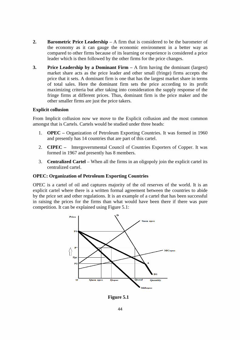
44

2. Barometric Price Leadership – A firm that is considered to be the barometer of

the economy as it can gauge the economic environment in a better way as

compared to other firms because of its learning or experience is considered a price

leader which is then followed by the other firms for the price changes.

3. Price Leadership by a Dominant Firm – A firm having the dominant (largest)

market share acts as the price leader and other small (fringe) firms accepts the

price that it sets. A dominant firm is one that has the largest market share in terms

of total sales. Here the dominant firm sets the price according to its profit

maximizing criteria but after taking into consideration the supply response of the

fringe firms at different prices. Thus, dominant firm is the price maker and the

other smaller firms are just the price takers.

Explicit collusion

From Implicit collusion now we move to the Explicit collusion and the most common

amongst that is Cartels. Cartels would be studied under three heads:

1. OPEC – Organization of Petroleum Exporting Countries. It was formed in 1960

and presently has 14 countries that are part of this cartel.

2. CIPEC – Intergovernmental Council of Countries Exporters of Copper. It was

formed in 1967 and presently has 8 members.

3. Centralized Cartel – When all the firms in an oligopoly join the explicit cartel its

centralized cartel.

OPEC: Organization of Petroleum Exporting Countries

OPEC is a cartel of oil and captures majority of the oil reserves of the world. It is an

explicit cartel where there is a written formal agreement between the countries to abide

by the price set and other regulations. It is an example of a cartel that has been successful

in raising the prices for the firms than what would have been there if there was pure

competition. It can be explained using Figure 5.1:

Figure 5.1

45

DD1 is the market demand curve of oil which is relatively inelastic as there is no

substitute of oil; Snon– opec is the supply curve of all those countries (firms) combined

together that have not joined the cartel and hence are competing with each other and the

cartel. It is also relatively inelastic as the supply of oil is also limited it being a natural

resource. It is obtained by the summation of the marginal cost of these firms and can be

seen that cost of Non– OPEC firms is quite high. Now the first step is to locate the

demand curve of the OPEC which is obtained by setting different prices and finding out

how much of the market demand would be left for the OPEC after the rest has been

supplied by the non– opec firms combined together. If OPEC sets the price as P1 which is

obtained from the intersection of market demand curve and supply curve of the Non–

OPEC then the whole market demand can be satisfied by them and hence nothing would

be left for the OPEC to supply. Thus here the demand from the OPEC is zero. If however

it sets the price at P2 which is so low that the Non– OPEC firms would not supply

anything then the whole market demand is to be fulfilled by the OPEC. It is shown by

point A on the market demand curve. Thus the demand curve of the OPEC is kinked

‘P1AD1’ and the corresponding marginal revenue curve is MRopec., marginal cost curve is

MCopec. The equilibrium price that would prevail in the market is given by MRopec =

MCopec which is the profit maximizing condition for OPEC that is the price maker. Thus

the equilibrium price is OP* at which the OPEC sells OQopec units and all the competitive

firms combined sells OQnon– opec such that

OQopec + OQnon– opec = OQtotal and

OQopec > OQnon– opec

To see whether OPEC has been successful or not we compare the price difference

between what OPEC has set and what would have been there if there was no cartelization

and all firms would have competed freely. In the latter case price would have been where

demand curve of OPEC and MCopec intersect. Thus, the difference is huge as shown by

the difference between P* and Ppc which shows significant monopoly power that OPEC

enjoys.

Long Run Effect of OPEC Action:

(i) OPEC action of restricting its output caused increase in supply of oil by non-

OPEC countries because of increase in price. This caused shift in supply curve of

these countries to the right. The share of OPEC declined. By 1985 it reduced to

30 percent. The price fell and in order to maintain price OPEC had to further

reduce its output.

(ii) Secondly the long run demand curve becomes more elastic as compared to the

short-run demand curve in above diagram. This is because people have to spend

their money more on insulation of oil heated buildings, economical diesel

engines etc. In the very long run more money was diverted for research to

develop more petroleum efficient and alternative technologies such as solar

technology etc. All these resulted in fall of OPEC exports. Production limitations

continued to maintain the price at high level.

46

(iii) Because of heavy reduction in output to maintain price OPEC started

experiencing fall in income. Disturbed by this development members started

violating their quotas and had to meet frequently to settle things. Ultimately

OPEC had to eliminate quotas by 1985. The price fluctuated before settling

clown in the 1990s.

OPEC experience tells that:

(i) It is highly profitable for competitive firms to form a cartel and behave like

monopoly in the short run by restricting output given inelastic demand curve.

(ii) In the long-run however, it becomes increasingly difficult to retain the monopoly

power and firms have to choose between short run and lone run profits

(iii) Also, in the long run it is not possible to continue output restrictions due to loss

in revenues and threat of breaking down of cartel.

CIPEC: Intergovernmental Council of Countries Exporters of Copper

CIPEC is a cartel of copper and captures only 30% of the copper producing countries of

the world. It is also an explicit cartel like OPEC where there is a written formal

agreement between the countries to abide by the price set and other regulations. As

against OPEC it is an example of a cartel that has been unsuccessful in raising the prices

of copper in the international market. It can be explained using Figure 5.2.

Figure 5.2

DD1 is the market demand curve of copper which is relatively elastic because of the fact

that there are substitutes of copper like aluminum etc. Supply curve of the Non– CIPEC

countries (firms) is Scipec that is also relatively elastic because of the fact that supply of

copper can be easily obtained from scrap etc. Demand curve and marginal revenue curve

of the CIPEC is obtained in the same manner as done for OPEC taking into consideration

the non collusive countries. The equilibrium price is set by CIPEC which is obtained

from equating marginal revenue and marginal cost of the CIPEC. It is point E where price

is set at OP* and quantity sold by CIPEC is OQcipec and by Non– CIPEC is OQnon– cipec.

47

Here it can be noted that quantity sold by Non– CIPEC is more than that of CIPEC as

CIPEC is a minority cartel where only 8 countries have joined the cooperation. The

monopoly power here is also very les as there is very small difference between the price

that would have prevailed in case of pure competition shown by Ppc and cartel price OP*.

So, we can conclude by saying that though OPEC has been successful in raising the

prices of oil in the international market but CIPEC has been unsuccessful at doing so, it

can be because of the following reasons:

1. OPEC is a big cartel that consists of majority of countries that produce oil

whereas CIPEC is a minority cartel where only few firms have joined the cartel.

2. OPEC is a cartel of oil whose demand and supply both are relatively inelastic

providing it a better scope for exploiting its monopoly power whereas CIPEC is a

cartel of copper whose demand and supply both are relatively elastic thus

providing lesser monopoly power.

3. The difference between cost of the cartel firms and competitive firms (those

which have not joined the cartel) is quite large as OPEC firms produce at a much

lesser cost whereas in CIPEC this difference is not quite significant.

These reasons have led to the success of OPEC and failure of CIPEC and from this we

can summarize few conditions that are required for successful functioning of cartel:

1. The demand for the commodity for which cartel has been made should be

relatively inelastic.

2. The firms that join cartel should be able to control majority of the world’s supply.

Centralized Cartel

This is an extreme form of cartel and rarely visible in real life as it assumes that all the

firms join the cooperation and none of the firms is outside the cartel. This cartel thus acts

as a monopoly where there is a centralized body that sets the price and quantity that is

equal to the monopoly and then allocates the total output and total profits amongst

different cartel members. If we assume that there are four firms in the market, and all

have same costs of production then the output and price determination can be shown

using Figure 5.3.

Dmarket is the total demand curve of the market and MR is the corresponding marginal

revenue curve. MCtotal is the summation of the marginal cost curves of the four firms

combined together. Equilibrium is obtained by the intersection of marginal revenue and

marginal cost curves and it is at point E where the price is OP* and quantity is OQt. The

centralized authority would distribute the output equally between the four firms such that

each firm sells OQt/4 output at a price of OP* per unit.

Above three cases of cartel showed that it is very difficult if not impossible for a cartel to

be successful as there is incentive for a firm to cheat on the cartel and earn even higher

profits than what it could have earned by being a member of the cartel. This has been

explained by a model of Game Theory known as Prisoner’s Dilemma.

48

Figure 5.3

5.4 PRISONER’S DILEMMA

Prisoner’s Dilemma is a model that explains how oligopolist firms could act to their

mutual disadvantage. The prisoner's dilemma is a paradox in decision analysis in which

two individuals acting in their own best interest pursue a course of action that does not

result in the ideal outcome. It shows why firms cheat and get a worse result than what

would have been if they would have cooperated. It is based on the concept of Game

Theory, a mathematical technique that helps in understanding the nature of

interdependence among rival firms that are faced with uncertainty in their pricing and

output decision. A game is described by its payoffs, strategies, number of players and

information available. Prisoner’s Dilemma can be explained with the help of following

case:

There are two friends A and B, who are suspects in a crime and are being interrogated in

separate rooms such that they cannot communicate with each other. The two strategies

available with them (to confess the crime or to not confess) with their respective payoffs

are given in the matrix below:

B

A

Confess Do not Confess

Confess B = 10 years

A = 10 years

B = 20 years

A = 2 years

Do not Confess B = 2 years

A = 20 years

B = 4 years

A = 4 years

Thus the matrix above reveals why A and B both have an incentive to cheat (confess)

while it would have been best for both of them to have cooperated by not confessing. If

both A and B confessed then both would get 10 years imprisonment. The best however

would have been where both do not confess and get away with 4 years of imprisonment.

49

If however one of them confesses while the other does not confess then the one who

confesses gets away with a lesser imprisonment of just 2 years. Thus both think that it is

best for them to confess thinking that the other would not confess and both get away with

10 years of imprisonment. This shows how prisoners thinking for their individual best

bring an outcome that is worse for them as well as for the group. The same can be applied

to the oligopoly where firms try to maximize their individual gains by cheating on the

other and hence get away with the profits that are worse for the group as a whole. The

above matrix can be modified to show the situation for oligopoly. If we assume that there

are just two firms C and D with the strategies available to them being that of to cheat or

not to cheat on the price being decided collectively.

D

C

Cheat Do not Cheat

Cheat D = Low Profits

C = Low Profits

D = Very Low Profits

C = Very High Profits

Do not Cheat D = Very High Profits

C = Very Low Profits

D = High Profits

C = Highs Profits

The matrix above revealed that if two firms C and D colluded, they could have fixed up

monopoly price and earned monopoly profits or high profits. If however a firm tries to

cheat on the cartel by charging a lower price assuming that the other firm would not cheat

and keep the price high as set by the collusion then the firm which cheats or lowers the

price earns very high profits and the firm that does not cheat earns very low profits. This

makes both the firms to cheat on the cartel and both the firms reduce the price and hence

they end up earning low profits.

The prisoner’s dilemma shows that oligopolists always follow a strategy that leads to

competition amongst firms and leads to lower profit. But if the game is repeated again

and again the outcome can change as firms may learn from their past outcome.


Check your progress


(a) Prisoner’s dilemma is a model based on Game Theory of mathematics.

(b) Both OPEC and CIPEC are examples of implicit cartels.

Ans. 1(T), 2(F)


(a) Prisoner’s dilemma shows why firms ……………. when it is beneficial for them

to ……………. .

50

(b) OPEC is a cartel of…………….

(c) For a cartel to be successful the demand of the product should not be perfectly

…………….

Ans 1. Cheat, Cooperate 2. Oil 3. Elastic.


1. Why OPEC has been successful in raising the prices while CIPEC has been

unsuccessful.

2. How Prisoner’s Dilemma can be applied to Oligopoly to show the non cooperative

behaviour of the rival firms.

5.6 GAME THEORY: EXAMPLE

Co-operative behaviour in oligopoly is a situation when firms jointly decide the prices

and output and maximizes their joint profit. This situation is called collusion, in this

situation it becomes profitable for one firm if it defects and cuts the prices and rises

output, as long as other do not do so, Non-cooperative behaviour is a situation when they

do not co-operate and decides their prices and output separately and compete with each

other. When firms in oligopoly do not co-operate it is called non-cooperative equilibrium

or Nash equilibrium (Named after US mathematician John Nash).

In oligopoly the basic dilemma the firms face is whether to co-operate or to compete.

If they co-operate profit will be maximum and if they do not profit for all will decrease.

Now we will see the behaviour of an oligopolistc firm through an example of game

theory. Game theory is the study of decision making in situations where strategic

interaction (moves and countermoves) between rival firms occurs. We will assume a case

of only two firms in the market, called Duopoly. The case is as follow:

Table 1: The Oligopolist’s dilemma: to co-operate or to compete.

Firm B’s Output

One-half Two-third

Monopoly output Monopoly output

One-half

Monopoly

output 20 20 15 22

Firm B’s Output

Two-third

Monopoly

output 22 15 17 17

51

The Table 1 above explains the dilemma faced by oligopolists of whether to co-

operate or to compete. It is called Payoff Matrix for a two firm duopoly game. The right-

side figures on each cell shows the profits of firm A and left side figures on each cell

show the profits of firm B (in Rs. Crores). It can be explained that if the two firms co-

operate and produce one half of market share each will earn Rs. 20 crores of profit. In

case of co-operation they can maximize their profits. If firm A defects and produces two

thirds of output and firm B produces half of monopoly output, then firm A will earn Rs.

22 crores and firm B Rs. 15 crores. Similarly, if firm B defects and produces two-third

and firm A produces one-half then firm B will earn Rs. 22 crores and firm A will earn

only Rs. 15 crores. If both decide to compete and produce two-third of monopoly output

each then profits for both will fall to Rs. 17 crores. This type of game, where they reach a

non-cooperative solution when they could co-operate, is called Prisoner’s Dilemma.

Prisoner’s Dilemma is shown below:

Table 2: The Prisoner's Dilemma

Mr. Ram

Confess Not confess

Mr. Shyam Confess 6 6 0 9

Not confess 9 0 1 1

Two prisoners Mr. Ram and Mr. Shyam are arrested for committing a crime and

interrogated separately. They are told the following:

(a) If both are claimed to be innocent, they will get a light sentence that is 1 year in

jail.

(b) If one confesses and the other does not, then who confesses will be released free

and the other will be punished for 9 year in jail, and

(c) If both confess, then both of them will get a-punishment of 6 years in jail.

The payoff matrix presented in Table 2 shows the dilemma of the prisoners about

whether to confess or not to confess. If none of them confess then both will get 1 year of

jail, but if Ram confesses and Shyam does not then Ram will be left free and Shyam will

get 9 year of imprisonment and the vise-versa. And if both of them confess then both will

get 6 years of imprisonment. Not confessing is the best solution in this game (Pareto

efficient solution) but this leaves one always in uncertainty. This solution is not a stable

solution as one gets an imprisonment of 9 years if he/she does not confess and the other

does. Therefore, confession dominates in the mind of both the prisoners. If both of them

confess then they end up with 6 years jail for both. This kind of equilibrium is called

Nash equilibrium. From both the figures above it is clear that it they co-operate then they

will earn the maximum profit than if they compete.

52

5.7 OLIGOPOLY AND THE FUNCTIONING OF THE ECONOMY

Oligopoly is an important market feature in modem economies. Oligopoly has played an

important role in modern economic growth. It is an emerging phenomenon in the

developing economies in recent time. Many industries are operating through oligopoly

market structure. The existence of economies of scale and economies of scope make

impossible for perfect competition and monopolistic competition to survive. Too many

firms cannot exist in such a situation. In the long-run oligopoly can be evaluated through

the following three questions:

1. The market mechanism under oligopoly

Under perfect competition, prices are determined by the forces of demand and

supply whereas prices are administered by the firms under oligopoly. Despite this

difference, Lipsey observes that, the market system reallocates resources in

response to change in demand and costs roughly by the same way under oligopoly

as under perfect competition.

2. Profits under oligopoly

Oligopolists either co-operate or compete in the market. They can maximize their

joint output and profit through co-operation, but one can always increase its

individual profit by defecting. High profit in the long-run can always attract the

new firms, unless natural and/ or firm created barriers exist to restrict entry of new

firms in the market.

3. Very long-run competition

To survive in the long-run, oligopolists keep on innovating to upgrade the quality

of product and minimize their cost of production. Each firm spends significant

amount on Research and Development to produce better quality’ at minimum

costs. Differentiated products with different character are available in oligopoly

market. Consumers get more choice in the market. Consumers get quality

products at competitive rates. Oligopoly market structure is more conducive to

economic growth in the long-run.

5.8 Contestable Markets and Potential Entry

The theory of contestable markets explains that in the long-run, abnormal profits earned

by oligopolists can be eliminated without actual entry. Potential entry can also affect the

market.as much as an actual entry does. It is possible only when the following two

conditions are fulfilled

1. Entry must be easy to accomplish: There should not exist any barriers to entry,

either natural or firm created.

2. The existing firms must consider potential entry while making price and

output decisions: The existing firms must react when new firms try to enter into

53

the market. They must cut their prices and sacrifice profits (short run) to restrict

the new entrants.

Contestable markets always expect potential entry because of huge profits earn by the

existing firms in the market. But entry to such markets is too costly. Fixed costs are very

high. To develop, design, and sale a new product in such a market involve huge sunk

cost. Sunk costs are those costs which cannot be recovered if a firm leaves the market

soon. Firms which produce multiple and differentiated products can easily distribute these

costs among those many products. For new firms, producing huge number of

differentiated products is not easy. Therefore, these costs are very high for a firm which

produces single product in the market.

If a new firm can enter and leave the market without any sunk costs of entry, such

markets are called perfectly contestable markets. A market can be perfectly contestable,

even if, firms have to pay some costs of entry if these costs are recovered when firms

leave the market. If the sunk costs are lower, the market will be more contestable and

vise-versa.

Sunk costs of entry constitute entry barriers. Higher the sunk costs, larger will be

profits earn by the existing firms. If the firms operate in the market without, large sunk

costs of entry, then they will not earn large profits. As part of strategy, existing firms

keep their prices as low as that can only cover the total costs. If they charge high prices

and earn abnormal profits then the new firms will enter and may capture the profits and

leave until it is vanished. Contestability forces the existing firms to keep the prices low.

Potential entry works as good as actual entry in a contestable market to limit the profits of

existing firms.


Oligopoly, a market structure that is most common in the real world consists of two

different categories – collusive and non-collusive. This chapter talked about collusive

oligopoly where collusion can be explicit where there is a proper written formal

agreement between the firms to decide the price and output that each firm would produce

and sell. Its most common form is Cartel, but this type of collusion is usually not allowed

by the countries’ legislation as it can lead to creation of monopoly that can exploit the

consumers. Two most famous cartels are OPEC – cartel of oil producing countries and

CIPEC – a cartel of copper producing countries. While OPEC has been successful in

raising the prices by cartelization, CIPEC is an unsuccessful cartel because of the reason

that demand, and supply of oil is relatively inelastic whereas that of copper is elastic. The

chapter also discussed about Implicit form of collusion that is price leadership by a

dominant firm where there is no agreement between the firms to collude but still firms

follow the price set by a leader firm as that avoids the uncertainty and reduces the

chances of a price war. However, in spite of the benefits of cartelization firms still cheat

as that brings them more profits and it has been highlighted by Prisoner’s Dilemma which

shows that why firms in an oligopoly cheat while they would have been better off if they

would have colluded.

Game theory is applied to explain co-operative and non-cooperative behavior of

oligopolistic firms.

54

TERMINAL QUESTIONS

1. Explain the features of oligopoly?

2. Explain the various co-operative and competitive behaviour of oligopolistic firms.

55

LESSON 6

CONSUMER AND PRODUCER THEORY IN ACTION

Sanjeev Grewal

St. Stephen’s College

Delhi


This lesson is divided into following parts:

Part I: Changes in supply in a competitive industry

Part 2: Changes in technology in a competitive industry

Part 3: Effects of taxation on competitive industry

Part I: Changes in supply in a competitive industry

The main aim of this part is to use the theory of competitive market behaviour to

understand some important real world problems. In particular, we shall see how the

economy responds in the short ran as well as in the long ran to shifts in supply that are

brought about by changes in the cost structure of an industry.

6.2 COST CHANGES

Costs for an industry can change for a variety of reasons.

1. A common reason for a change in costs for an industry is a change in the price of

some input used by the industry. We can think of several recent examples: Wheat

prices in India have gone up sharply since 2006. This has increased the costs for

several industries. For instance, restaurants and hotels, manufactures of bread and

biscuits etc. have seen their costs escalate in recent times as a result of the

increase in wheat price. Another example is provided by the sharp increase in

crude oil prices in the last few years. This has lead to an increase in costs for the

petroleum products industry and consequently for the transportation industry.

Another example that has been discussed a lot in the newspapers recently is the

effect of a sharp hike in cement prices witnessed in India since 2006 on the costs

for firms engaged in construction and infrastructure creation.

2. Technological changes might also lead to changes in costs. For example,

technological advances over the last few decades have drastically reduced the

costs of several industries. Computers and mobile phones are some of the

examples that immediately come to mind, if one wants to see evidence of a

dramatic reduction in costs over a very short span of time due to technological

advancement. However, there are times when use of a different technology in

order to reduce environmental damage might actually lead to an increase in costs.

This might explain why some advanced industrial countries are so vehemently

opposed to pollution control measures advocated by environmentalists.

56

3. Another common reason for a change in costs is a change in taxes paid by the

firms in the industry. In India, every year industry watchers eagerly wait for the

budget speech of the Finance Minister in the Lok Sabha to analyze the impact of

changes in excise and customs duties on a wide variety of industries like iron and

steel, cement, cars, petroleum products etc.

4. Acts of nature might also be an important source of costs changes for some

industries. Winter fog in Delhi, for instance, increases the costs for aviation

industry because it leads to delays in landing and take-off of aircrafts and

sometimes might even result in cancellation of flights. Massive rains that lead to

widespread flooding in Mumbai a few years ago resulted in an increase in costs

for the insurance industry. On the other hand, adequate rain in the months of July

and August in states like Punjab and Haryana might lower the costs of paddy

production for farmers since they might not be required to use diesel-run pump

sets for irrigation.

6.3 COMPARATIVE STATICS

In this lesson we use the comparative static technique. We start with a market that is in

long run equilibrium. We then introduce a cost change that leads the market to a new

equilibrium (that is a new state of rest or no change for the system when ail the

adjustments to cost changes have taken place). We compare these two equilibrium stales

to study the impact of cost changes. Comparative statics is to be contrasted with static

analysis that looks at equilibrium in a market that does not receive any external shocks or

disturbances (that is. a change in a variable fixed from outside). Both these methods are

to be contrasted with dynamic analysis that looks at the path of evolution of the state of a

system when it is not in equilibrium.

Long run response might be very different from what happens in the short run

We shall first see now the economy adjusts to changes in costs in the short run. In the

long run, however, the response of a competitive industry can be very different. We

analyze the long run response next. A large part of the difference in our analysis and

conclusions between the short run and long run effects is explained by free entry and exit

of firms in a competitive industry in the long run in response to abnormally high or low

profits.

Freedom of entry and exit of firms is one of the most important characteristics of

competitive markets. Most of the efficiency results of competition stem from this.

Freedom of entry and exit of firms lies at the heart of adjustment process in a competitive

market and we try to illustrate it in a wide variety of situations. At times our conclusions

are quite different from the answers of those who have not received a formal training in

economics. A little investment of time and energy on your part will, we hope, change the

way you think about major issues of public concern.

6.4 CHANGES IN INPUT PRICES

To begin with, we illustrate the general impact of a change in input prices on a

competitive industry by considering a specific example. We consider the impact of a

57

reduction in the price of wheat flour on the bread industry. Suppose each loaf of bread

requires a constant amount of wheat flour, say 200 gin per loaf of bread. If the price of

wheat flour declines, say by 5 Rs. per kg, the marginal and the average cost curves of a

typical bread factory decline by the same vertical amount (by one Rupee for all levels of

bread output).

This is shown in Figure 6.1. Notice that there is a parallel vertical shift in the average

and marginal cost curves in Panel B and the extent of vertical shift is the same. Assume

all firms in the industry have the same cost curves. The industry supply curve is obtained

by horizontally adding up each firm’s MC curve that lies above the AVC.

We start from a position of long run equilibrium. In Panel A of Figure 6.1, initial

industry equilibrium is at E0 where the industry demand curve D and initial industry

supply curve S0 intersect. The initial market price is P0 and the quantity demanded and

supplied in the industry is Q0.

Diagram 6.1

The corresponding initial equilibrium for a typical firm in the industry is at e0 in

Panel B of Figure 6.1, where price = MC = AC. Each firm supplies q0, a quantity at

which AC is minimized and every firm makes zero economic profit (that is, it earns

normal profits) and hence there is no incentive for an existing firm to exit or for a new

firm to enter the industry. Given our assumption about fixed input use per unit of output,

a reduction in price of wheat flour leads to a downward parallel shift of one Rupee in MC

and AC curves from MC0 and STAC0 to MC1 and STAG1 respectively. In general,

shifts in AC and MC are not parallel. As a matter of fact, while a cost reduction will

always lead to a downward shift in AC curve, though not necessarily a parallel one, the

MC might not shift down at all. This might happen, for instance, if only fixed costs

decline and variable costs remain the same.

Short run impact of a decline in input prices

Since each firm’s MC has shifted down, the industry supply curve also shifts down to S1,

market price falls to P1 and industry output rises to Q1 in Panel A of Figure 1. Notice that

the fall in market price is less than the one Rupee fall in costs given by P0P2, the vertical

distance between S0 and S1 in Panel A of Figure 6.1.

58

In Panel B we see that when the market price is P1 and the costs for each firm have

declined (by more than the decline in market price). Each firm in the industry increases

its optimal quantity supplied to q1 a level higher than the efficient one at which AC is

minimum. Moreover, each firm in the industry makes supernormal profits in the short run

since price is greater than AC. The area of the shaded rectangle in Panel B of Figure 1

gives the magnitude of this profit.

Long run impact of a decline in input prices

In the long run, however, in a competitive industry these positive economic profits will

attract new firms into the industry. As the number of firms in the industry rises, the short

run industry supply curve shifts to the right, the market price falls and the industry output

rises. This process continues till the short run industry supply curve has shifted to S2 and

the market price falls to P3, equal to the new minimum AC. The industry output rises to

Q2.

Fall in market price from P1 to P2 implies that each firm in the industry is now

producing output q0, the efficient level of output at which AC is minimum. Notice that q0

is less than q1, the output produced by an existing firm in the industry in the short run

after a cost decline. The entry of new firms pushes down the market price and hence leads

to disappearance of supernormal profits earned by the existing firms.

Long run Supply Curve of the Industry

An alternative way of analyzing the long run impact is to look at how the long run

industry supply curve shifts. With free entry and exit of firms and with identical cost

curves for all the firms, the long run industry supply curve is a horizontal straight line

whose vertical intercept is equal to the lowest AC for a typical firm. This is shown in

Pane! A of Figure 6.2 The long am industry supply curve shifts from S to S*. The market

price drops from P to P*, the full extent of drop in costs, and industry output rises from Q

to Q*.

In Panel B Figure 6.2, we see that each firm continues to produce output q, the

efficient output level, when market price and costs decline. Moreover, each firm

continues to make zero economic profits in the long run.

Diagram 6.2

In the long run, under perfect competition, the price declines by the full extent of the

decline in the lowest AC. The output is higher and the price is lower. The firms are still

59

making zero economic profits. All the benefits of lower input prices are passed on to

consumers.

Questions for Review

1. We discussed above the case of a reduction in input prices. Discuss the opposite

case of an increase in input prices. Carefully describe the short run and long run

impact on the industry as well as on a typical firm in the industry.

2. We discussed a special case of cost change above where both MC and AC curves

shifted down by the same vertical distance. We remarked that this need not always

happen. Discuss the short run and long run impact of a decline in fixed costs on

the industry as well as on a typical firm in the industry.

(Hint: The MC curve for a firm will not shift at all.)

(a) What happens to price and quantity in the short run?

(b) What happens to profits of the firms in the industry in the short run?

(c) Are there any incentives for entry of new firms in the industry?

(d) What is the new long run equilibrium?

Part 2: Changes in technology in a competitive industry

In this part we try to learn how a change in the technology for the production of a good

affects its market. Preferences and technology are the basic building blocks from which

demand-and supply curves are derived. In economics we normally take technology and

preferences as exogenous (that is, we regard them as given from outside). Changes in

technology, however, have important economic implications. In this lesson we study the

impact of exogenous changes in technology within the framework of competitive

markets.

6.5 CHANGES IN TECHNOLOGY

We shall first see how the economy responds in the short run as well as in the long ran to

shifts in supply that are brought about by technological changes in an industry.

We noted in the previous lesson that technological changes are frequently major

sources of changes in costs in the real world. In this lesson we analyze the short run and

long- term impact of two kinds of technological changes.

1. A once-for-all-change in technology

2. A continuous process of technological change

A once-for-all-change in technology

Assume that the industry starts from a situation where there has been no change in

technology for a long time and all firms have the same cost curves. Further, suppose that

the industry is initially in a state of long run equilibrium.

60

This is shown in Figure 6.3 We start from a position of long run equilibrium. In Panel

A of Figure 6.3, initial industry equilibrium is at E0 where the industry demand curve D

and initial industry supply curve S0 intersect. The initial market price is P0 and the

quantity demanded and supplied in the industry is Q0.

Diagram 6.3

The initial equilibrium for a typical firm in the industry is at e0 in Panel B Figure 6.3,

where price = MC = ATC. Each firm supplies q0, a quantity at which ATC is minimized

and every firm makes zero economic profit (that is. it earns normal profits) and hence

there is no incentive for an existing firm to exit or for a new firm to enter the industry.

61

Notice that P is greater than AVC, hence the firm is making positive operating profits (the

difference between total revenue and total variable costs) that just cover its fixed costs.

Now suppose that a single advance in the industry’s production technology takes

place that lowers the costs of production for newly built plants. We assume that existing

plants can’t take advantage of this technological advance since the new technology has to

be embedded in new plant and equipment. In the very short- run there will be no change

in the industry since it takes time to build new plant and equipment.

In the medium run, since new technology lowers the average total cost curve to ATC1

and the original price P0 was equal to the average total cost for the existing plants; new

plants are profitable and will be built soon. With this capacity expansion, the industry’

supply curve shifts to the right to S1, market price falls to P1 and industry output rises to

Q1 in Panel A of Figure 6.3 Notice that capacity expansion and fall in market price

continues till price has fallen to the lowest AC for the new plants and further entry is not

profitable,

At price P1, the new plants are operating at the most efficient scale where they are

producing an output at which AC is minimized. Firms with new plants are making zero

economic profits since their operating costs just cover their fixed costs. This is shown in

Panel C of Figure 6.3.

Firms with old plants, however, will not be covering their total costs. If the costs for

the new plants are sufficiently lower than that of the old plants, the new market price PI

will be lower than minimum AVC of old plants. Old plants will be shut down

immediately and all surviving firms will use the new technology.

A more interesting case, however, is where the new market price P1 is higher than

minimum AVC of old plants. This is shown in Panel B of Figure 6.3. At price P1 firms

with old plant produce output q2, a level of output at which price = MC and since price is

less than ATC, each Urn; with an old plant makes a loss given by the area of rectangle

P1CDE. It is, however, optimal to produce output q2 since price is higher than AVC and

the firm is making an operating profit given by the area of the rectangle ABC P1. Had the

firm shut down its loss would have been higher. Its revenue would have been zero, it

would still have to incur the fixed cost of production (given by the area of the rectangle

ABDE) and losses would have been greater since the firm would not have been able to

use its operating profits to at least partially offset its fixed costs.

Old plants will continue to coexist with new ones and firms with old plants will be

making losses. A non-economist might think that operating loss-making old plants is

inefficient and it would be advantageous to discard them. He could not be more wrong!

As long as old plants recover their variable costs, it is optimal to operate them. Fixed

costs are sunk; they can’t be avoided by shutting down old plants. One of the first lessons

in economics is to ignore sunk costs. Let us try to understand this by looking at an

example from everyday life. If you go to a restaurant and happen to order a lousy meal,

don’t force it down your throat just because the price you paid is very high. You have to

pay the price whether you finish the meal or not. It is a sunk cost. The decision whether to

62

eat all of what you ordered or to leave it in the plate depends not on the size of the bill

(you have to pay that in either case), but on whether not eating (or eating something else

or somewhere else and paying something additional for it) makes you happier than eating

what is in front of you. Let bygones be bygones.

With the passage of time, however, old plants will wear out. They will now be

replaced by plants using new technology. At the time of replacement, the cost of plant is

not sunk. Profit maximizing firms will choose plants with lower costs. Plants with old

(higher-cost) technology will gradually disappear. In the long run a new equilibrium will

be attained in which all plants use the new technology. As shown in Panel A of Figure 6.3

output will be Q1, higher than output Q0 in the original equilibrium. Price will be P1

lower than P0 in the original equilibrium. The new plants will be operating at an efficient

scale and will be just covering their costs.

All the benefits of lower costs due to technological advancement will be passed on to

the consumers in the long run.

Ongoing technological change

We can generalize the analysis of the previous section to consider the outcome in a

competitive industry where there is a continuous technological change. Plants built today

have lower costs than plants that were built in the past. However, costs are expected to be

even lower for plants that might be built at a future date.

It is clear from the analysis of previous section that ongoing technological progress

will lead to a continuous process of entry of newer lower cost firms. The market price

will continually decline. However, older plants will not necessarily be shut down as soon

as plants with better and lower cost technology make an appearance. Owners of old plants

will continue to operate them as long as they cover their variable costs.

This situation is described in Figure 6.4. The Plant shown in Panel A of Figure 6.4 is

the oldest plant that is on the margin of shutdown. It is making a loss since market price

is lower than its average total cost. The plant is just covering its AVC and is indifferent

between shutting down and continuing to produce output q1. If the price drops any

further, the plant will be shut down.

63

Diagram 6.4

The plant shown in Panel B is using an intermediate technology. It is also making a

loss, but it is covering at least some pan of its fixed costs (shown by the shaded area) in

addition to covering all its variable costs by producing its optimal level of output q2.

The plant shown in Panel C is the one that uses the newest technology and has the

lowest costs. It not only covers its fixed costs (notice that price is higher than its AVC),

but it also makes a profit (price is higher than its ATC) for the time being by producing

its profit maximizing output, q3. Since the potential entrant firms know that technological

progress is continuous, they will enter the industry only if they make positive profits at

the lime of entry that will compensate them for the losses they expect to make in the

future when newer firms with lower cost technology will enter the industry and push

down the price.

The point made above about the link between modernization and economic efficiency

needs to be emphasized. Older plants have higher costs and firms using them might be

making losses. At the same lime there are firms in the industry that operate newer plants

and have lower costs. These firms are making profits. Is this compelling evidence of

economic inefficiency on the part of firms using the old plants? Is it true that firms using

older loss-making plants should discard them immediately and modernize their plant and

equipment? Is doing so profitable for these firms? Is it welfare enhancing for the society?

It should be clear from our analysis above that the answer to all these questions is not

necessarily in the affirmative. It is efficient to use older loss making plants as long as they

cover their variable costs. They produce goods that are valued more by the consumers

than the resources currently used up by operating the old plants (their variable costs). It is

in the interest of the firms with old plants and also in the social interest to continue to use

these old plants as long as the variable costs are covered.

Another point to be noted is that market price paid by consumers is determined not by

the average costs of (he old inefficient plants, but by the costs of the firms with the

newest and the most efficient plants. Entry of firms with the most efficient technology

64

into the industry will continue and supply will keep on increasing till the price has

dropped to a level where latest entrants can barely cover the opportunity cost of their

capital over the expected lifetime of their plants. It implies that new entrants today must

earn positive economic profits for some time to offset the losses that they expect to earn

later when firm’s with even more efficient technology enter the industry and push down

the market prices to a level lower than the ATC of these current entrants. The full benefit

of new technology is passed on to the consumers as soon as begins to get used by the new

entrants even though a vast majority of firms in the industry might still be using old

technology. The price paid by the consumers depends only on the costs of the most

efficient firms. As Paul Samuelson once said, it is the tail that wags the dog in economics.

Owners of older firms have to sell their goods at the same lower price that is charged by

the new firms. Their operating-profits keep on declining as entry of lower cost firms

keeps on driving down the market price. These firms will ultimately quit the industry

when they can’t even cover their variable costs.

This brings us to the final point that we want to make in this lesson. The concept of

economic obsolescence is different from that of physical wear and tear. We emphasized

above that old machinery should not necessarily he discarded just because firms using it

have higher costs and might even be making losses since market price depends on the

costs of the most efficient firms. Just as one should not be overenthusiastic about

discarding old machinery, one should not continue to use an old machine because it is

still functional. When the price drops below average variable costs the machine is

economically obsolete even though it may not be physically worn out. Old capital

equipment is obsolete and should not be operated if by using it the firm can’t even cover

the variable costs. This might happen well before the equipment is physically worn out.

The concept of economic efficiency should be understood both by those who have a

fetish for new technology and want to discard old equipment as soon as they see

something more; modern and also by those who would never discard old equipment, as

long as it works.

Questions for Review

1. In what sense are the benefits of technological progress passed on to the consumer

in a competitive industry? Would your answer change if entry to the industry were

restricted?

2. How would your answer to the first question be modified, if the new technology is

patented and only one firm can use it?

3. In reality firms have to spend money on research and development to generate

technological progress. Use your answer to questions 1 and 2 to present an

economic case for patents.

65

6. 6 PART 3: EFFECTS OF TAXATION ON COMPETITIVE INDUSTRY

There are various kinds of taxes that the government imposes which ultimately affect the

costs of firms and industry. We will consider three different types of taxes-per-unit tax,

lumpsum tax and profit tax.

(1) Per-unit tax: It is a tax that is levied on each unit produced by the firm. In a way it

can be said to be another cost to the firm. As a result of per unit tax (say sales tax)

the marginal cost of the firm shifts up by the amount of the tax. At the industry

level the supply curve shifts up by the amount of the tax. Accordingly, the effects

of a per-unit tax on output of a competitive industry can be listed as follows:

(i) In the short run the price of the output will rise but by less than the amount of

the tax. So, the tax burden will be shared by consumers and producers. The

consumers pay higher price than before and producers do not cover their

average total costs.

(ii) In the long run, some firms who don’t cover their costs may leave the

Industry. The industry will contract (fall in size) and losses will disappear. If

the cost curves of existing firms remain unaffected due to contraction of the

industry then price will rise by full amount of the tax. In such a case the

burden of the tax will be totally on the consumers. This also implies that

government intervention in the competitive industry may affect its size,

volume of sales and price in the short run but it cannot influence its long-run

profitability effects of per-unit tax is shown in the diagram below.

Diagram 6.5 Diagram 6.6

Diagram 6.5 shows effect of per-unit tax on price and quantity by shifting the

supply curve upwards. The original equilibrium point is E0 with price P0 and

quantity Q0. Due a per-unit tax supply shifts from S0 to S, so that new

equilibrium is now at point E1. Tax equals S0S1 or E1T or P1P2. Price increases

to P1 Since increase in price is P0P1 which in less than the tax E1T, the tax

burden is shared by consumers and producers in the short run. After tax quantity

has also fallen to Q0.

66

In Diagram 6.6 the effect of per-unit tax is shown by shifting the demand curve

down by the amount of tax. It shows that after tax producer gets price P2 after tax

which is less than the market price P1.

(2) Lump-sum tax: Lump sum tax is a kind of fixed cost of the firm and increases

the total cost of the firm and industry. The marginal costs and marginal revenues

remain unaffected. The average cost curve shift up due to tax at the existing level

of output. Lumpsum tax reduces the revenue. As long as the firm is able to

recover its variable costs it will remain in business otherwise it will shut down in

the short run lumpsum tax does not affect price and output in the short run.

However, in the long run some firms, who do not cover their increasing costs

leave the industry and the size of the industry will fall. Price will rise and output

will fall until the whole of tax burden is passed on to the consumers.

(3) Tax on profits: From the economists, point of view the firm in perfect

competition earns normal profit or zero economic profit in the long run. So, on

this basis a tax on profits will neither affect price nor output of a competitive

industry in equilibrium. So, it will also not affect allocation of resources.

However, in reality profits are defined in tax laws according to accountants, usage

which includes returns to capital, reward for risk-taking and could be taxed.


In this lesson you have learnt the following:

1. The cost of competitive firm and industry changes due to change in input price,

change in technology and imposition of taxes.

2. Change in input price (rise/fall) causes change in supply (fall/rise) and change in

MC (rise/fall).

3. Improvement in technology causes increase in supply and fall in average cost of

competitive industry and firm and vice versa.

4. Imposition of per unit tax causes decrease in supply (upward shift) and decrease

in demand (downward shift).

6.8 TERMINAL QUESTIONS

1. Explain effect of per unit tax on price and quantity from the demand side of the

market?

2. Explain effect of per unit tax on price and quantity from the supply side of the

market?

67

LESSON 7

MARKET FAILURE

7.1 LEARNING OBJECTIVE


(a) Identify the situations that lead to market failure

(b) Understand the concept of Public Goods

(c) Compute the impact of Externalities

(d) Identify the situations that lead to Moral Hazard and how it can be reduced.

7.2 INTRODUCTION

The aim and objectives of market should be as follows:

1. There should be efficient production of goods by making use of the available

resources. It being assumed that there are only two factors of production that is

labour and capital and their quantity is fixed, both have to be optimally utilized to

produce two commodities. Here the efficient production would be only if it is not

possible to increase the production of either one or both the commodities without

reducing the production of the other.

2. The goods being produced should be efficiently distributed amongst the

consumers in the economy. This happens only when the distribution amongst the

consumers is such that it is not possible to increase the satisfaction of one

consumer without decreasing the satisfaction of the other. This happens when the

indifference curves of the two consumers are tangent to each other, the marginal

rate of substitution being same for both the consumers.

3. The output mix should be efficient such that the output that is distributed amongst

the consumers in such a manner that the marginal rate of substitution and

marginal rate of transformation are equal.

In an economy having perfect competition all the above conditions are automatically

fulfilled. However, such an economy rarely exists and it gives rise to imperfections in

the economy and non optimal allocations which would be discussed in the current

chapter. But let us understand and explain the efficiency of perfect competition.

7.3 ALLOCATIVE EFFICIENCY UNDER PERFECT COMPETITION

Allocation efficiency refers to the situation where allocation of resources lead to

maximum gain to the society reflected in maximization of the sum of consumers and

producers surplus.

Consumer surplus is the difference between the total value which the consumers are

willing to place on all the units consumed of the product and the actual payment that they

make on its purchase.

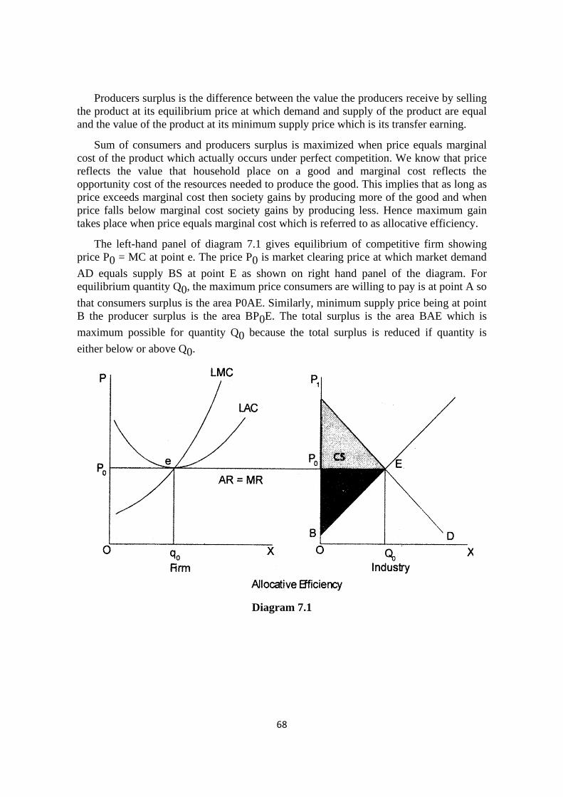
68

Producers surplus is the difference between the value the producers receive by selling

the product at its equilibrium price at which demand and supply of the product are equal

and the value of the product at its minimum supply price which is its transfer earning.

Sum of consumers and producers surplus is maximized when price equals marginal

cost of the product which actually occurs under perfect competition. We know that price

reflects the value that household place on a good and marginal cost reflects the

opportunity cost of the resources needed to produce the good. This implies that as long as

price exceeds marginal cost then society gains by producing more of the good and when

price falls below marginal cost society gains by producing less. Hence maximum gain

takes place when price equals marginal cost which is referred to as allocative efficiency.

The left-hand panel of diagram 7.1 gives equilibrium of competitive firm showing

price P0 = MC at point e. The price P0 is market clearing price at which market demand

AD equals supply BS at point E as shown on right hand panel of the diagram. For

equilibrium quantity Q0, the maximum price consumers are willing to pay is at point A so

that consumers surplus is the area P0AE. Similarly, minimum supply price being at point

B the producer surplus is the area BP0E. The total surplus is the area BAE which is

maximum possible for quantity Q0 because the total surplus is reduced if quantity is

either below or above Q0.

Diagram 7.1

69

7.4 MARKET FAILURE

Market failure refers to failure of market mechanism to achieve efficient allocation of

resources in the economy allowing a smooth circular flow of income. There are several

factors responsible for market failure. They are-

(i) lack of competition among firms and presence of market power in the form of

oligopoly or monopoly which is also called imperfect competition. There is

presence of excess capacity in these markets and price exceeds marginal cost

causing allocative inefficiency by reducing consumers and producers combined

surplus.

(ii) Provision of public goods whose consumption cannot be only restricted to those

who can pay for them and common property resources whose owners are none

but users are everybody.

(iii) Problems of externalities in both consumption and production wherein action of

one agent affects another in the society.

(iv) Asymmetric information which creates a situation where one party to a market

transaction has fuller knowledge of it consequences than is available to the other

party. For example in the market for secondhand car only the seller knows the

actual condition of the car and buyer has no information on the quality of the

product.

(v) If there are missing markets i.e. needed markets do not exist at all.

Market failure does not mean that nothing good is happening in the market but it means

that the best possible outcome has not been attained. It arises in the following cases:

1. Asymmetric Information

2. Insurance Market

3. Market Signaling

4. Moral Hazard Problem

5. Principal Agent Problem

1. Asymmetric information – Asymmetric information means that the buyers and

sellers do not possess the same set of information, one having a better or more set

of information as compared to the other and hence is better off. The problem is

also known as Lemons Problem given by Ackerlof. A ‘lemon’ is a derogatory

term for a poor quality second– hand car. However, the lemon's problem has

many wider implications in terms of understanding information failure in general.

It can be explained with the help of an example:

Example 1 – Let us assume that there is a car dealer who deals in second hand cars and is

aware about the conditions of the car and does not pass on the entire information to the

buyers. Here the car dealer is thus having better and more information and takes the

advantage of the information by selling the cars at a higher price then what they are worth

70

off. The buyers would purchase it once but after becoming aware about the situation of

the second hand cars would not go for it the second time at the same price as they are

suspicious of the seller’s intention and hence the market and demand for second hand cars

reduces because of asymmetric information as all the good quality cars are driven out of

the market because of the lesser price being paid for it and only low quality cars would be

left in the market. After a short period, it can be predicted that all cars sold on the second

hand car market will be lemons. When applying this concept to other markets it can be

suggested that, whenever there is information failure, there is the possibility that markets

will become lemons markets. If so, the supply of good quality products will fall and the

supply of poor quality will products rise.

This problem of asymmetric information can be reduced by getting more information like

in the above case the buyers can get the second hand cars evaluated by an independent car

evaluator to find the correct status and price of the used cars.

2. Insurance market – Here also the problem is because of asymmetric information

but unlike the used cars here it is buyer of the insurance policy that is in

possession of better and more information. It also leads to adverse selection as can

be explained using the following example:

Example 2 – Let us assume that it is the case of a medical insurance where the buyer of

the policy has more information about his health, the premium set by the insurance

company is according the average individual that includes both the healthy and unhealthy

individuals but it is the unhealthy ones that are more likely to go for insurance and it

increases the losses of the insurance company because of which the premiums increase

and it further rations out the healthy individuals out of the insurance market as they are

not willing to buy the insurance at such high premiums. Thus the market now has only

unhealthy individuals which further increase the losses and hence forces the insurance

companies to go out of the market. This is also because of asymmetric information.

3. Market signaling – The problem of adverse selection can be reduced or even

eliminated by market signaling where in the producer gives signals about better

quality of its products to the buyers thereby preventing the outflow of such goods

from the market as happened in the Lemons’ problem. Thus the buyers are able to

differentiate between high quality and low quality products and it gives the sellers

an advantage as they are able to sell high quality products at a higher price. This

can be done by branding the product or providing guarantees and warranties that

assures the buyer about the quality of the product and helps in reducing the

suspicion that buyers have about seller’s description of the product or service.

4. Moral Hazard problem – This problem generally arises in case of insurance

where if an individual is insured then there are greater chances of him being

negligent about the subject matter of the insurance. Moral hazard refers to a

situation where you do not behave in a manner that you are expected to in case

there has been no one else to share the loss. For example if an individual gets his

building insured for fire then if he does not take proper care to ensure that there is

no fire then it is a case of moral hazard. Similarly where an individual after taking

medical insurance does not take preventive measures for his health also leads to

issue of moral hazard. It leads to market failure as if moral hazard is not reduced

71

or eliminated than it leads to increased premiums of insurance thereby defeating

the very purpose of insurance. The issue of moral hazard cab be tackled by going

for Coinsurance wherein the insurance company bears a part of the loss and the

rest is borne by the beneficiary himself. For example in case of an insurance by an

individual wherein the insurance company would bear 70% of the losses subject

to a maximum limit then in case of the mishappening the remaining 30% of the

total loss is borne by the insurance policy holder and only 70% is made good by

the insurance company. Thus, in this case as the entire loss is not covered up by

the insurance company the beneficiary is bound to take care which he would have

otherwise not assumed. Another way is to ensure that enough precautions have

been taken to avoid the loss, for example in case of fire insurance even after

taking the insurance it has to be made sure that enough safety provisions were

made and loss is unavoidable. However, if the insurance company finds out that

enough safety provisions were not there then no compensation of loss is made to

the policy holder.

5. Principal agent problem – In a modern world there is separation of ownership

and management where the principal or the owners are the shareholders whereas

the organization is managed by the agents or the managers. Because of this

separation of ownership from management arises the principal– agent problem.

The problem arises because of the distinction in the requirements and interests of

the principal and agent whereas owners wants maximum profits or total present

value of the firm, the managers are usually interested in their self interests that is

increased salaries, reputation etc. For example, the shareholders of firms, the

principals, usually delegate responsibility for day– to– day decision making to

appointed managers, the agents. This creates a situation of asymmetric

knowledge, with managers knowing much more than the shareholders, and raises

the possibility of inefficiencies, especially when shareholders and managers have

different objectives. To avoid the conflict and ensure that the organization is

working for the best interest of the owners extra cost is incurred in terms of

monitoring costs that reduces the efficiency which would have been there without

these extra cost burden. The problem can be reduced to a certain extent by

providing incentives to the managers to work in the best interest of the owners by

providing them with Golden Parachutes or linking their incentives with the

fulfillment of owners requirements.

7.5 EXTERNALITIES

Till now all the chapters and the discussions are concentrated on the buyer and the seller,

there is however a third party also that is affected by the production and/or consumption

of the goods or services though not being directly a part of the production or exchange

process. the impact on such third party is known as externality as it is external to the

parties that are directly involved in the generation process. Such effects can be positive or

negative that is beneficial or harmful, the former being external benefit and the latter

being external cost. A simple example of external benefit can be getting oneself

immunized for a communicable disease; it is called external benefit as it will reduce the

spread of the disease to others who have not got themselves immunized. External cost can

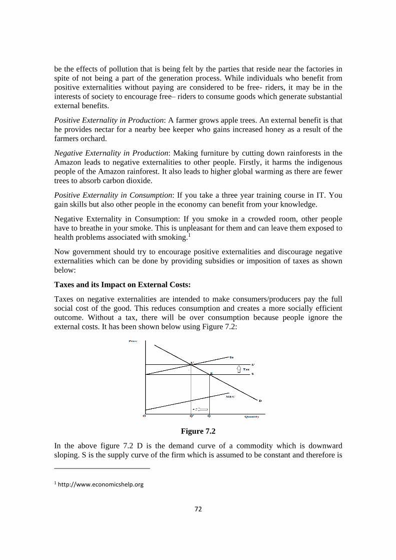
72

be the effects of pollution that is being felt by the parties that reside near the factories in

spite of not being a part of the generation process. While individuals who benefit from

positive externalities without paying are considered to be free- riders, it may be in the

interests of society to encourage free– riders to consume goods which generate substantial

external benefits.

Positive Externality in Production: A farmer grows apple trees. An external benefit is that

he provides nectar for a nearby bee keeper who gains increased honey as a result of the

farmers orchard.

Negative Externality in Production: Making furniture by cutting down rainforests in the

Amazon leads to negative externalities to other people. Firstly, it harms the indigenous

people of the Amazon rainforest. It also leads to higher global warming as there are fewer

trees to absorb carbon dioxide.

Positive Externality in Consumption: If you take a three year training course in IT. You

gain skills but also other people in the economy can benefit from your knowledge.

Negative Externality in Consumption: If you smoke in a crowded room, other people

have to breathe in your smoke. This is unpleasant for them and can leave them exposed to

health problems associated with smoking.1

Now government should try to encourage positive externalities and discourage negative

externalities which can be done by providing subsidies or imposition of taxes as shown

below:

Taxes and its Impact on External Costs:

Taxes on negative externalities are intended to make consumers/producers pay the full

social cost of the good. This reduces consumption and creates a more socially efficient

outcome. Without a tax, there will be over consumption because people ignore the

external costs. It has been shown below using Figure 7.2:

Figure 7.2

In the above figure 7.2 D is the demand curve of a commodity which is downward

sloping. S is the supply curve of the firm which is assumed to be constant and therefore is

1 http://www.economicshelp.org

73

horizontal straight line parallel to X axis, it is the marginal private cost of production of

the firms and does not include the external costs. MEC is the marginal external cost curve

which is upward sloping as with an increase in output the external cost also increases, for

example if we assume that the external cost is the pollution that firm makes when it

carries out production then it will increase as the production increases. The total cost of

production is obtained by summation of private cost and external cost which gives Ss

supply curve that is parallel to MEC. The equilibrium that firm derives is where demand

and supply curve given by private cost intersects that is at point E, where the firm

produces OQ level of output. However, the firm’s equilibrium should be at point E’

where demand and total cost that includes both private and external cost are equal. The

firm should reduce its output to OQ’. This can be done if government imposes tax on the

firm which increases the private cost of production to S’ and reduces the output to the

desired level and with the tax revenue government can carry out the task of pollution

control thereby reducing the impact of externality.

Subsidies and its Impact on External Benefits:

Figure 7.3

In figure 7.3, D is the demand curve that the firms take into consideration for determining

their equilibrium level of output; it includes only the marginal private benefit. MEB is the

marginal external benefit and S is the supply curve of the firm derived from the marginal

cost. The equilibrium is where demand and supply curves intersect that is at point E

where the firm is producing OQ level of output. But this is not what the firm should be

actually producing as it is not taking into account the external benefit into account. Ds is

the demand curve after adding the marginal private benefit and marginal external benefit

and the actual output that should be produced should be where Ds and S intersect it is at

point E’ and firm should be producing OQ’. To increase the output government can

provide subsidy that reduces the cost of production and supply curve shifts downwards to

S’ and output increases to OQ’. Thus, increase in the output brings an increase in the total

external benefit.

7.6 PUBLIC GOODS

Generally, a commodity that is supplied by the government is known as public good but

in economics the term is somewhat different as for a good to be called public good it

should fulfill the following two characteristics:

74

1. Non-Rival – Consumption by one consumer does not restrict consumption by

other consumers – in other words the marginal cost of supplying a public good to

an extra person is zero. If it is supplied to one person, it is available to all.

2. Non-Excludable – The benefits derived from public goods cannot be confined

solely to those who have paid for it. Non– payers that is those who have not paid

anything for the production of the commodity too can enjoy the benefits of

consumption at no financial cost and economists call this the 'free– rider' problem.

This leads to market failure as once the commodity is produced it can be enjoyed

by all and therefore there is problem in the initiation that is who will pay for it.

The derivation of equilibrium in case of a public good is different from that of the market

demand curve as here the market demand is not obtained by the horizontal summation of

the individual demand curves but by the vertical summation of the individual benefits

derived by the persons enjoying the benefits of the public good this is because of the fact

that once one unit of public good is produced it can be enjoyed by all. It has been shown

in Figure 7.4.

Figure 7.4

Here let us assume that there are two consumers A and B and there, demand curves that

shows marginal private benefit are DA and DB correspondingly. To get the market

demand curve or the total demand curve we need to add the two individual demand

curves vertically that gives DS as the demand curve. the equilibrium is where DS

intersects MC and it provides that OQ units of output would be produced in the economy

that would give the benefit of OA’ to consumer A and OB’ to consumer B. Public goods

are not normally provided by the private sector because they would be unable to supply

them for a profit. It is up to the government to decide what output of public goods is

appropriate for society. To do this, it must estimate the social benefits from making

public goods available. Because public goods are non– excludable it is difficult to charge

people for benefiting form a good or service once it is provided. The free rider problem

leads to under– provision of a good and thus causes market failure.


Check your progress


(a) Moral Hazard is a problem that usually arises in case of insurance.

75

(b) Public goods are the goods being produced by the government.

(c) Free riders problem arises because of usage of a commodity by the non payers.

(d) External costs can be reduced by granting of subsidy.

(e) Externalities are not taken into account by the producer while determining the

equilibrium.

Ans. 1(T), 2(F), 3(T), 4(F), 5(T)


(a) The combined demand curve in case of public good is obtained by…………..

summation of the individual demand curves.

(b) Free Riders is the problem associated with………….. .

(c) A public good is one that has two important characteristics ………….. and

………….. .

(d) Problem of moral hazard to a certain extent can be reduced by going for

………….. .

Ans 1. Vertical 2. Public Goods 3. Non rival and non excludable 4. Reinsurance.


1. How equilibrium is obtained in case of Public goods?

2. What is market failure and under what conditions there is a situation of market

failure?

3. How equilibrium is obtained in case of Externalities.

4. Explain the concept of Lemons problem.

5. Explain why the combined demand curve of public goods is vertical summation of

the individual demand curves?

7.8 FUNCTIONS OF GOVERNMENT

1. Basic functions of government: According to Classical economist Adam Smith

government must-perform two basic duties:

(a) government must protect the society from the violence and invasion of other

independent societies

(b) government must protect, as far possible, every member of the society from

injustice or oppression of every other member of it. In the sphere of economy

this implies that government must provide security of property and define and

enforce property rights that give people a secure claim to the fruits of their own

labour and allow markets to function efficiently. These property rights include

effective legislation on consumption and production rights, working of

institution such as insurance companies, banking, stock exchanges and joint

stock companies etc. Accordingly, it is the responsibility of the government to

76

regulate and control monopoly tendencies and ensure allocative and productive

efficiency the way they exist under a perfectly competitive market.

7.9 PUBLIC POLICY TOWARDS MONOPOLY AND COMPETITION

We have already seen that monopoly is allocatively inefficient because of lower output

and price being higher than marginal cost which cause dead weight loss to the society.

This calls for government intervention. Government intervention can take several forms

as given below.

(i) Government may ask monopoly firm to produce at a price equal to marginal

cost. This is not a problem if the monopolist continues to earn profit at marginal

cost pricing. But in case of natural monopoly marginal cost pricing will create

losses to the firm. (See diagram below)

In panel-1 of diagram 7.5 if government controls the price at p0 which is equal

to marginal cost at point-E there is still profits for the monopolist since at this

price average cost is C1 which is less. So, profit is P0C1, per unit of output.

Here the government successfully controls the monopolist who also survives in

the market by getting some profit.

But in case of a natural monopoly (panel-2 of diagram 7.5 marginal cost pricing

lead to loss because at price P0 = MC average cost C1 is more so that loss in

C1P0 per unit of output. Natural monopolies emerge in the provision of public

utilities where of a single firm can supply the market output.

Diagram 7.5

(ii) Even controlling price at average cost level may be inefficient again for natural

monopoly. As in panel-2 of diagram 7.5 P1 is average cost price which is higher

and the corresponding output, is below competitive level of Q0.

(iii) Since both marginal cost and average cost pricing do not yield desired result for

natural monopolies, they are directly taken over by government itself in many

countries.

77

(iv) Technological changes have made many natural monopolies behave like

competitive industry. So, government policies must adjust itself to continuous

technological change.

(v) Due to failure of government as business organization there have been a wave of

privatization recently in many countries including India. Many nationalized

industries have been privatized in UK. Disinvestment of public sector units in

India is another example. While allowing privatization to be implemented

rapidly governments are also creating public regulatory authorities to look into

the functioning of these natural monopolies. In UK example of such bodies are

OFTEL (Telephones), OFGAS (gas) etc. Security Exchange Board of India

SEBI in a regulatory body in India. Privatization reduces governments’ role in

business and allows innovations to take place faster. It is expected that

government’s intervention as controller and regulator must allow competition to

grow among firms.


Economics generally revolves around demand and supply of a commodity that is used to

determine the equilibrium price and quantity but while doing so they do not take into

consideration the external costs and benefits that the third party incurs because of the

production and/or consumption process. These are known as externalities and if it is

external costs then government should try to reduce the usage by imposition of tax and in

case of external benefit the usage should be increased by granting subsidies as that is the

true equilibrium. Another important concept that was discussed in the chapter was that of

the public goods which is not same as the goods produced by government but are the

commodities that are non rival and non excludable. Public goods also lead to market

failure as it brings the problem of free riders where in once a commodity is being

produced one cannot stop the nonpayers from taking its benefit. Various other causes that

lead to market failure are moral hazard, principal agent issue, Lemons problem and so on

and the solution is reinsurance, golden parachutes etc.

Government intervenes to regulate monopolies and other imperfect markets to ensure

allocative and productive efficiencies the way they exist under perfect competition.


1. Give the meaning of market failure. What are the causes of market failure?

Explain.

2. Differentiate between positive and negative externalities with the help of

examples? How can they be dealt with to ensure better market outcomes?

3. What are the features of public goods? How are the public goods responsible for

market failure? Determine the efficient amount of public good that should be

produced?

78

LESSON 8

MARKET FOR FACTOR INPUTS DEMAND AND SUPPLY OF FACTORS

8.1 INTRODUCTION

The total output of an economy is the result of the joint productive efforts of the various

factors of production; land, labour, capital and enterprise. This total output ultimately gets

distributed among the factors that contributed to its production in the form of wages, rent,

interest and profit. The purpose of the theory of distribution is to explain the principles

that govern this distribution. The distribution of total product depends on how the various

factors are priced in the market. Thus, pricing of the various factors of production is the

subject matter of the theory of distribution.

There are two aspects of the factorial distribution of national income; (i)

determination of the per unit prices of the different factors and (ii) the division of the

national income as between the different factors, i.e., absolute and relative shares of

different factors in national income. The first question is essentially a micro-economic

problem concerning the determination of equilibrium at the level of an individual firm or

an industry. The second question concerns the factorial distribution of income at the level

of the economy and, therefore, forms part of macro analysis. Thus, we have micro and

macro theories of distribution. In the present set of lessons we are concerned only with

the micro theories of distribution i.e., the question of factor-price determination.

Just as the price of any commodity is determined by the interaction of the forces of

supply and demand, similarly the price of a factor is determined by the interaction of the

forces of supply and demand for it. The theory of distribution is, thus, a special case of

the theory of price determination discussed in the earlier set of lessons. However, the

supply and demand for factors exhibit some peculiarities which have to be taken into

account while considering the pricing of particular factors. Herein lies the justification for

a separate theory of factor price determination. Let us first examine the demand for and

supply of factors in some detail.

8.2 THE DEMAND FOR FACTORS

1. The Nature of the Demand for a Factor

Why does a producer demand a factor? The demand for a factor is derived (or indirect)

and not direct demand. The demand for a commodity is direct in the sense that it directly

satisfies some human want. The demand for a factor, on the other hand, is not direct in

this sense. A factor is demanded not for its own sake, but simply because it can contribute

to the production of some commodity demanded by the consumers. For example, a

farmer pays rent for the use of land simply because it helps to produce, let us say, wheat

which is demanded by the consumers. Similarly, he pays for seeds and fertilizers because

they help to produce commodities, which are demanded by the consumers.

When a producer employs an additional unit of a factor it yields him some extra

output. While demanding a factor, the producer is not so much interested in the extra

output that it yields him as in the amount of the extra revenue he will get from the sale of

79

that output. In other words, he demands a factor simply because it ultimately contributes

to his revenue. Hence the price a producer will be willing to pay for a factor unit will

depend upon the addition to his total revenue which results from the employment of an

additional unit of that factor. The additional revenue yielded due to the employment of an

additional unit of a factor is called the marginal revenue product (MRP). For example,

suppose that by employing 10 labourers on a given plot of land a farmer gets 100 quintals

of wheat which sell for Rs. 20,000 in the market and by employing 11 labourers instead

of 10 he is able to raise 110 quintals of wheat which sell for Rs. 22,000. It is evident that

due to the employment of an additional labourer total revenue of the producer rises from

Rs. 20,000 to Rs. 22,000. Rs. 2000 is, thus, the MRP of the 11th unit of labour. While

demanding a factor the producer has his eyes set on this quantity. It is in this sense that

the demand for factors is derived out of the demand for the commodities that they help to

produce.

2. Different Concepts of Marginal Product

There are three different senses in which the concept of marginal product (MP) is used.

Firstly, it may be used to express the addition made to the total physical product of a

producer due to the employment of an additional unit of a factor, the amounts of all other

factors remaining constant We call this additional physical product as the marginal

physical product (MPP). For example, if by employing 11 labourers on a given piece of

land instead of 10, the total wheat output of a farmer increases from 200 quintals of rice

to 220 quintals, then the MPP of the 11th unit of labour will be said to be 20 quintals.

Thus, the MPP of a factor is the addition made to the total physical output of a producer

due to the employment of an additional unit of a factor while keeping the amounts of all

other factors constant.

Secondly, the concept of MP may be used in value productivity sense. The addition to

the total revenue of a producer made by the employment of an additional unit of a factor,

with amounts of all other factors remaining constant, is called the marginal revenue

product (MRP) of the variable factor in question. According to this above example, the

total physical product of the producer increases from 200 quintals to 220 quintals when

he employs 11 labourers instead of 10 on the same plot of land. Now if the total revenue

of the producer increases from Rs. 40,000 to Rs. 42,000 when he sells 220 quintals

instead of 200, the MRP of the 11th labourer will be said to be Rs. 2,000.

It is evident that the MRP of a factor depends upon two things: (a) the additional units

of output produced and (b) the contribution of each unit of output to the total revenue of

the producer. The additional output produced by the employment of an additional unit of

a factor is called the MPP and the contribution of an additional unit of output to the total

revenue of a producer is called the marginal revenue (MR). Thus:

MRP = MPP × MR

Thirdly, the concept of marginal product may also be used to denote the market value

of the MPP of a factor. For instance, the MPP of the 11th labourer according to the above

example is 20 quintals of wheat. Now if the ruling market price of wheat, when the larger

output is sold (220 quintals instead of 200 quintals) is Rs. 200 per quintal, the market

value of the additional output will equal Rs. 4,000, Rs. 4000 then will be said to be the

80

value of marginal product (VMP) of the 11th labourer. VMP is simply the MPP

multiplied by the market price of the commodity. As already explained in the context of

the theory of firm, market price and average revenue (AR) are one and the same thing.

Thus:

VMP = MPP × AR

3. Relation between MRP and VMP

MRP equals MPP × MR while VMP equals MPP × AR MPP is common to both

concepts. MPP, as discussed in detail in Set VI of this paper, depends solely on the

technical conditions of production while MR and AR depend upon the structure of

commodity market where the firm sells its output. If the firm sells its output on a

perfectly competitive commodity market, it will be faced with a perfectly elastic demand

curve and its AR and MR will then be identical. Thus, in the event of perfect competition

in the commodity market the MRP (=MPP × MR) and VMP (=MPP × AR) of a factor to

a firm will be the same because AR and MR are identical. But if the firm is faced with an

imperfectly competitive commodity market, then MRP and VMP will not be the same. In

the event of imperfect competition in the commodity market, as we have already studied,

MR will necessarily be less than AR. From this it follows that in the event of imperfect

competition in the commodity market, MRP (which equals MPP × MR) will necessarily

be less than VMP (which equals MPP × AR) because MR is less than AR. Thus, in

conclusion we note that in case of perfect competition in the commodity market MRP

equals VMP and in case of imperfect competition MRP will necessarily be less than

VMP. Thus:

MRP (=MPP × MR) VMP (=MPP × AR) in case of perfect competition in commodity

market.

MRP (=MPP × MR) < VMP (=MPP × AR) in case of imperfect competition in the

commodity market.

We clarify the point further with a simple example. Suppose the total physical product

of a fanner per year increases from 200 quintals to 220 quintals of rice when he employs

21 labourers instead of 20, on a given piece of land. The MPP of the 21st labourer,

according to this example, would be 20 quintals. Further suppose that the farmer sells his

output on a perfectly competitive commodity market so that the price of rice remains

constant at Rs. 100 per quintal even when he sells the larger output. MRP of the 21st

labourer in this case would equal the change in the total revenue of the producer due to

the sale of the larger output i.e., 220 × 100-200 × 100 = 22000–20000 = Rs. 2000. VMP

(MPP × AR) in this case would also equal Rs. 2000 (=20 × 100 = 2000). Now suppose

the fanner is faced with an imperfect commodity market so that he is able to sell the

larger output at Rs. 98 per quintal and not at Rs. 100 per quintal. In this case MRP of the

21st labourer would equal 220 × 98 – 200 × 100 = 21560 – 20000 = Rs. 1560. And VMP

would equal MPP (=20) × AR (=Rs. 98) = Rs. 1960. Why is MRP in this case smaller

than VMP? The reason is very simple. When the price falls from Rs. 100 to Rs. 98, this

reduction in price applies not only to the extra output but also to the earlier output (i.e.,

200 quintals) which was earlier sold at Rs. 100 instead of Rs. 98. Thus, while the

producer gets additional revenue from the sale of the extra output (=20 quintals) at the

81

current market price equal to Rs. 1960, at the same time he suffers a loss in his earlier

total revenue equal to the fall in price (i.e., Rs. 2) multiplied by the earlier total output

(i.e., 200 quintals) i.e., output but also to the earlier output (i.e., 200 quintals) i.e., Rs.

400. The MRP (or the net addition to the earlier total revenue of the producer) would thus

equal Rs. 1960 – Rs 400 = Rs. 1560. Thus as a general rule we note that in the event of

imperfect competition in the commodity market MRP will be less than VMP by the

amount of loss of revenue suffered by the producer on his earlier output due to the fall in

price. In the present case when, in order to sell the larger output (220 quintals instead of

200. quintals), price falls from Rs. 100 to Rs. 98, he is compelled to sell the earlier output

(200 quintals) also at Rs. 98 per quintal and thus suffers a loss of revenue of Rs. 400/-.

Therefore, MRP of 21st unit will be less than its VMP by Rs. 400.

4. The Shape of the MRP Curve

The demand for a factor is derived from its MRP. MRP, as we have seen above depends

upon MPP and MR. The behaviour of MRP will thus depend upon the behaviours of its

components with changes in the quantity of the variable factor employed. Under a given

set of conditions the behaviour of MPP is determined by the operation of the law of

diminishing returns (or the law of variable proportions). The law states that as more units

of a variable factor are used with a given amount of other factors, after a point its MPP

starts diminishing, provided there is no change in the state of technology. We can explain

this law with a simple numerical example. Imagine a farmer employing more and more

labourers on a given plot of land. The table below records total, average and marginal

products as the farmer employs more and more labourers on the given plot of land and

other equipment etc.

TABLE 8.1

No. of workers Total Product Average Product Marginal Product

(In physical units)

1 15 15 15

2 36 18 21

3 60 20 24

4 92 23 32

5 120 24 28

6 144 24 24

7 161 23 17

8 176 22 15

9 189 21 13

10 189 19 0

11 176 16 –13

The figures in the above Table 8.1 show that both the average and marginal products

increase at first and the decline. The marginal product falls faster than the average. The

82

important point to note is that with the employment of the fifth unit the marginal product

starts diminishing. The same phenomenon is depicted in the diagram below.

In the diagram 8.1 below the MPP curve rises till the employment of OA units of

labour and thereafter it falls continuously. The APP curve rises till the employment of OB

units and thereafter starts declining. The relationship between APP and MPP is the same

as that between AC and MC explained in the earlier set of lessons.

Diagram 8.1

Diagram 8.2

In order to convert the MPP curve into the MRP curve we need to know the

contribution to revenue made by the MPP at each level of employment of the factor. It

bears repetition to point out at this stage that while MPP depends entirely on the technical

conditions of production, its value productivity depends upon the commodity market

where the firm sells its output. If the firm sells its output on a perfectly competitive

market, its MR will equal its AR and thus the MRP curve can be derived from the MPP

curve simply by multiplying the MPP corresponding to each level of employment of the

factor by the given market price of the product (AR). Diagram 8.2 depicts the MRP curve

corresponding to the MPP curve of the Diagram 8.1.

Carefully note the fact that just like the MPP curve the MRP curve is also downward

sloping. The reason for this is the diminishing marginal productivity of the factor. Also

note the fact that in this particular case MRP curve is also the VMP curve.

However, as already explained, if the firm is confronted with an imperfectly

competitive commodity market, it will be able to sell larger outputs only by reducing the

market price so that MR will be less than AR. As a result two things happen. Firstly, as

the firm is able to sell its extra output at a lower price, the VMP curve (which is derived

from the technically given MPP curve by multiplying MPP corresponding to each level of

employment of the factor by the market price of the product) will fall more sharply than

the MPP curve. Secondly, since MR will be less than AR, the MRP curve will lie below

the VMP curve and slope more sharply than the latter. Diagram 8.3 depicts the VMP and

MRP curves of a firm selling its product in an imperfectly competitive commodity

market.

83

Diagram 8.3

The difference between MRP and VMP is further explained with hypothetical figures

given m Table 8.2 below.

TABLE 8.2

Difference between MRP and VMP under Perfect

and Imperfect Competition in the Commodity Market

Units of Total MPP. Perfect Competition in theImperfect Competition in

the

the Factor Product Commodity Market Commodity Market

Pirce T.R. M.R.P. V.M.P. Pirce T.R. M.R.P. V.M.P.

1 15 15 100 1500 1500 1500 100 1500 1500 1500

2 36 21 100 3600 2100 2100 99 3564 2064 2079

3 60 24 100 6000 2400 2400 98 5880 2316 2352

4 92 32 100 9200 3200 3200 97 8924 3044 3104

5 120 28 100 12000 2800 2800 96 11520 2596 2688

6 144 24 100 14400 2400 2400 95 13680 2160 2280

7 161 17 100 16100 1700 1700 94 15134 1454 1598

8 176 15 100 17600 1500 1500 93 16368 1234 1395

9 189 13 100 18900 1300 1300 92 17388 1020 1196

10 197 8 100 19700 800 800 91 17927 539 728

Explanatory Notes:

1. MPP = Difference between two successive total products.

84

2. T.R, = Total revenue = Total product × price at which it is sold:

3. MRP = Marginal revenue product = Difference between two successive total

revenues.

4. VMP = Value of MPP = MPP × the price at which total product sells.

Carefully note the following:

1. Total product and MPP figures are the same because they are determined purely

by-technical factors.

2. In case of perfect competition in the commodity market, MRP and ‘VMP figures

are identical,

3. In case of imperfect competition in the commodity market MRP is always less

than VMP.

5. Firm’s Demand Curve for a Factor

Just as it is true that a profit maximizing firm, whether it is selling its product under

conditions of perfect competition, imperfect competition or monopoly, will produce to

the point at which its MC equals its MR, so it is true that a profit-maximizing firm will

purchase units of a variable factor up to the point at which the addition to its total cost

resulting from the employment of an additional unit (i.e. marginal factor cost, MFC)

equals the M.RP of the factor in question. Thus, in the purchase of a single variable factor

a firm will be in equilibrium when MFC equals MRP of the factor.

Thus, in equilibrium:

MFC = MRP

(1)

The above is a perfectly general equilibrium condition applicable to all market

situations. If we further assume that the firm is able to purchase any amount of the factor

without influencing market price (i.e, purchases in a competitive factor market), the MFC

of the factor to the firm is simply the market price (AFC). Therefore, for firms that

purchase their factor supplies in a perfectly competitive market the above equilibrium

condition (1) can be alternatively stated as follows:

AFC = MRP

(2)

This condition allows us to derive a firm’s demand curve for a factor from the MRP

curve. The factor’s MRP curve shows different MRPs corresponding to the different

amounts of the factor employed with given amounts of all other factors, Firm’s demand

curve for a factor would show the different amounts of the factor that the firm would be

willing to purchase at different prices of the factor. Therefore, when a firm purchases its

factor supplies in a competitive factor market (so that MFC = AFC) the MRP curve of the

factor becomes the firm’s demand curve for the factor as shown in the diagram below.

In the diagram 8.4 amount OA of the factor equates its MRP at point a with the price

OW. Therefore, at OW price the firm would be willing to purchase OA amount of the

factor. Amount OB of the factor equates its MRP at point b with price OWS. Therefore,

85

with OW, as the price the firm would be willing to purchase OB amount of the factor.

Similarly, at OW2 price the firm would be willing to purchase OC amount of the factor.

However, at this stage let us carefully note that the MRP curve is the firm’s demand

curve for the variable factor in question on the assumption that the price of the product

and the price of the factor are both given for the firm.

Diagram 8.4

6. Market Demand Curve for a Factor

In the preceding diagram the MRP curve is the firm’s demand curve for the factor in

question on the assumption that changes in the price of the factor do not, directly or

indirectly, affect the price of the commodity produced and hence the given MRP curve.

This assumption would be valid only if all other firms in the industry keep their outputs

fixed. However, this is not a realistic assumption. In the event of a fall in the price of a

variable factor we would expect all firms in the industry to employ more of this relatively

cheaper factor. This would increase the total output of the industry and cause the price of

the commodity to fall. A fall in the price of the commodity would cause the MRP curves

of all the firms (based on the higher price of the commodity) to shift leftward. Firms will

adjust their purchases of the factor with reference to the new MRP curve (corresponding

to the lower commodity price). Thus, each fall in the price of a variable factor (via its

effects on the factor’s total employment, total output and hence the price of the

commodity produced) will give rise to a new lower MRP curve with one equilibrium

point corresponding to the new factor price. The line joining such equilibrium points on

the different MRP curves will be the firm’s demand curve for the variable factor in

question when the reactions of other firms in the industry to changes in the price of the

factor are allowed for. This is shown in the diagram 8.5.

Diagram 8.5

In diagram 8.5 let us start from an equilibrium position such as point a on the curve

MRP, with OW as the factor price and OA as the amount demanded of it by the firm.

86

Now suppose the price of the variable factor falls from OW to OW1. All firms in the

industry employ more of this factor, as a result total output of the commodity increases

and consequently price of the commodity falls. Fall in the price of the commodity (say,

from Rs. 100/- to Rs. 98/-) causes the MRP curves of all firms to shift leftward. Suppose

as a result of these indirect effects the MRP, in the diagram above shifts position MRP2

with MRP2 and OW1 as the factor price equilibrium is established at point b with OB as

the amount demanded of the factor 0. Similarly, when the price of the factor rails further

to OW2, MRP2 shifts leftward to the position of MRP3 on which equilibrium with the

lower factor price (OW2) is established at point c; with OC as the amount demanded of

the factor. The line DD joining equilibrium points such as a, b, c, etc., is the firm’s

demand curve for the factor when reactions of other firms in the industry’ to variations in

the price of the factor are allowed for.

The lateral summation of the demand curves of all firms for a factor, as. derived

above, gives us the market demand curve for the factor in question. Just like the firm’s

demand curve, the market demand curve for a factor will also be downward sloping.

7. Firm’s Demand Curve for a Factor when factor Market Imperfect

As explained earlier, equality of MRP with MFC of a variable factor determines a firm’s

equilibrium in the purchase of a single variable factor under all market situations.

However, a firm’s demand curve for a factor, defined as indicating the different amounts

of the factor demanded by the firm at different prices of the factor, is based on the

assumption that MFC of the factor to the firm equals its price (AFC) so that equality of

MFC with MRP also means the equality of price of the factor (AFC) with MRP. This

implies that the firm purchases its factor supplies in a perfectly competitive factor market

so that it is able to purchase any amount of the factor without influencing the given

market price and as a result MFC of the factor equals its AFC. We derived the individual

and the market demand curves in the preceding sub-section on the basis of this

assumption. However, if a firm does not purchase its factor supplies in a perfectly

competitive factor market, it will be able to purchase larger amounts of the factor only at

higher prices. When a firm purchases larger amounts of a factor at higher prices, MFC of

the factor will necessarily be higher than its AFC. For example, if in order to purchase 51

instead of 50 units of a factor a firm has to raise the factor price from Rs. 100 to Rs. 102,

the MFC of the additional unit to the firm will equal Rs. 202 (102 × 51- 100 × 50 = 202)

which is greater than AFC.

When the MFC of a factor to a firm is greater than its AFC, it cannot afford to equate

MRP with the AFC because in doing so it will incur a net loss equal to the excess of MFC

over AFC and thus reduce its profits. In such a case the MRP curve cannot be described

as the firm’s demand curve for the factor in the sense of indicating the different amounts

of the factor demanded by the firm at different prices of the factor. Even in such cases

MRP curve will be described as the firm’s demand curve for a factor but in a different

sense which we will explain in a later section.

87

8.3 SUPPLY OF FACTORS

I. Supply of Factors to the Whole Economy

At first glance it may appear that quantities of most factors are fixed in an economy. For

example, there is an upper limit to the number of workers. Similarly, there are upper

limits to quantities of coal, oil, copper, iron ore, etc., available in the economy. However,

in practice we are never near these limits. Often a large undiscovered or unexploited

quantity exists, and a shortage of the resource that raises its price encourages exploration

and the development of previously unprofitable sources. Thus, the supply of a resource to

the economy usually varies considerably with changes in the price of the resource. With

this brief introduction we now come to a discussion of the characteristic features of the

supplies of individual factors.

2. Supply of Land

Land in economics includes all natural resources provided free by nature. The quantity of

a particular natural resource existing in the world is, of course, limited. But we are never

near these upper limits. Generally large undiscovered (or unexploited) sources exist and a

shortage that raises their prices encourages exploration, research and development of

previously unprofitable sources. Therefore, the supply of any natural resource usually

varies considerably with changes in its price, A high return to land provides incentives for

the development of its productive powers through irrigation, drainage, fertilization, etc.,

which greatly increase the supply of arable land. On the other hand, if the return to land is

low, its fertility may be allowed to be exhausted within a short period of time.

Traditionally, however, the supply of land (which includes all natural resources besides

mere space) to the whole economy has been assumed to be absolutely inelastic.

3. Supply of Labour

By the supply of labour (or the supply of effort) we mean the total number of hours of

work that the population is willing to supply. The supply of effort depends upon the

following factors,

(1) The size of the population: The size of the population sets the upper limit to the

total of labour, While there is some evidence that the birth and immigration rates are

higher in good times than in bad times, it is doubtful, especially in advanced economies,

whether economic factors are of paramount importance in determining the growth of

population. It is difficult to establish any definite relationship between the reward of

labour and growth of population. The reasons for which population varies are at the

moment largely unexplained. Therefore, for our purpose we may take the size of

population as fixed.

(2) The proportion of the population willing to work: The proportion of the

population entering the labour market varies considerably in response to variations in the

wage rate. Generally, arise in the wage rate results in an increase in the proportion of the

population willing to work. Women, old people and even young boys are induced to join

the labour force when the wage rate is high. For example, the proportion of married

women and old persons in the labour force increased dramatically during the Second

World War. In addition to the rate, the proportion of the population entering the labour

88

market also depends on the age composition of population, social institutions, customs

and distribution of wealth in the economy. For example, the extent to which women,

especially married women, enter the labour market partly depends on customs and

opportunity. Customs and opportunity can vary from one time to another and from one

place to another even within the same country. Greater equality in the distribution of

property in a society, by reducing the number of those who live on unearned incomes and

consequently do not need to work, will increase the supply of labour in an economy,

(3) The number of hours of work offered by each individual worker: By hiring

out his services a labourer gets some money as his wage, With this money he purchases

goods and services for his consumption. Thus, the labourer trades his leisure for goods,

by giving up leisure (i.e., by working) he gets money, and hence, goods. A rise in the

wage rate means that there is a change in the relative price of goods and leisure. Leisure

becomes dearer- relative-to goods (since each hour of leisure consumed now is at the cost

of more goods forgone), or alternatively, goods become cheaper relative to leisure since

each hour worked (i.e., leisure traded for goods) now results in more goods than before.

In the context of the theory of consumer’s demand we noted that a consumer tends to

substitute a cheaper good at the cost of a dearer good when their relative prices change.

The same logic applies to change in the wage rate also. Due to rise in the wage rate goods

be come cheaper relatively to leisure and as a result a labourer tends to substitute goods at

the cost of his leisure; he tends to have more goods by reducing his leisure. This is known

as the, ‘substitution effect’ of wage increase.

The substitution effect of a wage increase will tend to expand the supply of effort in

two ways. Firstly, some of those who were not willing to work at the lower wage rate

would now like to work because leisure has now become costlier in terms of goods

forgone. Secondly, for the same reason those who were already working would now like

to put in more hours of work per day or per week by reducing their leisure. Thus, the total

supply of effort will tend to expand due to these two factors.

Quite apart from the substitution effect discussed above, a wage increase also

generates an income effect. With an increase in the wage rate a labourer grows richer than

before even if he continues to work the same number of hours per day or per week as he

did when the wage rate was lower. Being richer the worker would demand more of all

normal goods including leisure. He will spend a part of the increase in his real income in

the purchase of leisure. He can do so by reducing the number of hours worked. So, the

income effect of a higher wage rate induces the worker to reduce the number of hours

worked per day or per, week. Thus, the substitution and income effects of a wage increase

tend to pull in opposite directions; the substitution effect tending to increase the number

of hours worked while the income effect tending to reduce the number of hours worked.

The net effect of a wage increase on the supply of effort will, therefore, depend on the

relative strengths of the two opposing tendencies. If the substitution effect is stronger than

the income effect, labourers will put in longer hours of work in response to a rise in the

wage rate. Bat if at any stage income effect becomes stronger than the substitution effect,

labourers will put in shorter hours of work consequent upon arise in the wage rate. The

supply curve of effort in this case will be backward rising as the one shown in figure

below.

89

In figure A of diagram 8.6 below as the wage rate rises from W1 to W2 and then to

W3. The supply of effort expands from OA to OC and then to OD. In other words, upto

the wage level W3 substitution effect is stronger than the income effect and as a

consequence supply of effort expands in response to increases in the wage rate. But when

the wage rate rises beyond W3 the income effect becomes stronger than the substitution

effect and consequently the supply curve of labour starts sloping backwards to the left. In

the figure B of diagram 8.6 when the wage rate increases from W3 to W4 instead of

expanding, the supply of effort actually contracts from OD to OB.

Diagram 8.6

Concluding our discussion of the supply of effort we can say that the backward rising

supply of effort curve presents a strong possibility but cannot be taken as the typical case.

There is no conclusive evidence available in support of a backward labour supply curve.

Therefore, we assume that normally labour supply curve will be upward rising bending.

4. Supply of Capital

Capital is a man-made factor of production and interest is its cost. The supply of capital

in a country consists or the existing machines plants, equipment, buildings, etc., and is

called the Capital Stock. In the course of production during the year a part of the existing

capital stock is used up and to that extent the supply diminishes. On the other hand, new

machines, buildings, plant and equipment are produced every year which go partly to

replace the worn-out part of the capital stock and partly to add to the stock. Ignoring

cyclical fluctuations, the supply of capital has been increasing over time in all modern

economies.

5. Supply of factors to particular uses

Different factors of production can normally be put to alternative, uses. Only few

resources may be specific to a particular use and that too only in the short run. A given

piece of land can be used to grow a variety of crops. Similarly, a labourer can be

employed either to weave cloth in a factory or to build a road or to dig a canal or to grow

various crops on a farm. Therefore, factors have to be allocated among various competing

industries and among different firms in the same industry in a rational manner.

Factor owners choose the use for their resources in which they earn the most. They, of

course, take many other things into account besides monetary benefits. Factors move

among different uses until there is no net advantage in further movement. A change in the

90

relative price paid to a factor in two uses leads factor owners to increase the quantity

supplied to the use in which the relative price has increased and to decrease the quantity

supplied to the use where it has decreased. This means that higher the (relative) price

offered to a factor in a particular use, the larger will be the amount of the factor supplied

to it. This gives rise to an upward rising supply curve to an industry as shown in the

diagram below.

SS curve in the diagram 8.7 is the supply curve of a factor to an industry. It is upward

rising indicating that higher the price offered to the factor, larger is the quantity supplied

to the industry in question. For example, when the price offered is OW1 only OA amount

of the factor is supplied.

Diagram 8.7

But when the price offered rises to OW2, amount supplied increases to OB. And

when the price offered rises to OW3 amount supplied increases further to OC.

As explained previously, the supply curve of any factor to the economy as a whole

will be normally more than perfectly inelastic. However, even in a case where the supply

curve of a factor to the economy as a whole is perfectly inelastic (as for example,

classical economists assumed the supply of land to be), its supply to a particular industry

will not be perfectly inelastic, it will be more classic because the industry will always be

able to attract more units of the factor from other industries by offering a slightly higher

price. Therefore, the supply curve of a factor to an industry will normally be more elastic

compared to its elasticity of supply for the whole economy.

6. Supply of a factor to an individual firm

In a factor market a firm may be either one of a large number of purchasers or one of the

few purchasers of a particular factor. If the firm is one of a large number of purchasers of

the same factor, its purchases will constitute a negligibly small fraction of the total

market supply of the Factor. As a result, the firm would be able to purchase any amount

of the factor at the going market price. In other words, the supply of the factor to such a

firm will be perfectly elastic at the price determined by the forces of market supply and

demand for the factor. As already explained, when the supply of a factor is perfectly

elastic, price (AFC) and marginal factor cost (MFC) to the firm are identical. On the other

hand, if the firm in question is one of the few big purchasers of a factor, its purchases will

constitute a sizeable fraction of the market supply of the factor and as a result when the

firm buys a large amount of the factor, its price is raised. Thus, in such a case the firm is

91

able to buy more units of the factor only at higher and higher prices. The supply curve of

the factor to the firm in such a case will rise upward. When the supply curve is upward

rising, as already explained, MFC is higher than AFC and therefore, the MFC curve lies

above AFC curve.

We may conclude our discussion by observing that normally the supply of all factors

to an economy is responsive to factor prices in the long run. In the short run the same

factor can have supply curves ranging from the vertical (i.e., perfectly inelastic supply

curve) to the horizontal, depending on which demand curve is coupled with supply-the

demand curve of a small firm, of an industry (or a big firm) of a group of industries (i.e.,

the whole economy). This is shown in the diagram 8.8.

It is thus evident that even when the supply of a factor to the economy as a whole is

rigidly fixed (as in fig. A below), it will be more elastic to a particular use (as shown in

fig. B), and will be perfectly elastic to a small user of the factor (as shown in fig. C).

Diagram 8.8



1. In the economic sense factor supplies for the economy as a whole are never

perfectly inelastic except, possibly, in the very short run.

2. Supply of a factor to an industry is generally more elastic than its supply to the

whole economy,

3. Supply of a factor to a small user of the factor can be assumed to be perfectly

elastic.


1. What are the determinants of demand for factor? Derive individual and market

demand curve of factor?

2. What are the determinants of supply of factors in the economy and for firms?

Discuss.

92

LESSON 9

FACTOR PRICING



(a) Understand the concept of Factor Pricing

(b) Differentiate between pricing of commodity and factors of production

(c) Establish the equilibrium in pricing of factors

(d) Comprehend the Marginal Productivity Theory.

9.2 INTRODUCTION

Till now all the chapters have discussed about output market that is how equilibrium price

of a commodity is determined by the analysis of its demand and supply, this chapter

concentrates on the input market that is how pricing of the factors of production that are

used to produce the commodity is determined. It is not only dependent on the demand and

supply of the factor itself but also on the productivity of the factor. There is however few

differences between the pricing of a commodity and a factor of production like:

1. Demand for a factor of production is not direct but indirect demand as it is

dependent on the demand for the commodity for which it is used. If there is no

demand for that commodity then the factor too would not be demanded. For

Example: If a particular type of labour is used in manufacture of tyres and if

demand for tyres increases then the demand for the labour too would increase and

vice versa.

2. Demand for a factor of production is joint demand as no commodity can be

produced by using just one type of factor of production. A particular combination

of different factors of production is needed to produce a commodity. Though the

factors of production can be substituted for each other but this substitution is not

infinite.

As done in the commodities market that there can be various types of market structures

starting from perfect competition on one extreme and monopoly on the other extreme,

similarly in the factor market too price determination is done under the following

conditions:

1. Perfect competition in both the product (commodity) market and factor market.

2. Imperfect Competition in product market and perfect competition in factor

market.

3. Perfect Competition in product market and imperfect competition in the factor

market.

4. Imperfect competition in both product and factor market.

93

Pricing of a factor of production say land, labour, raw material or other inputs is

explained by Marginal Productivity theory given below:

9.3 MARGINAL PRODUCTIVITY THEORY

Marginal Productivity Theory, a significant work that explains how factors of production

are priced was given at the end of 19th century and its main contributor was John Bates

Clark who proposed that a business firm would be willing to pay a productive agent only

what he adds to the firm’s well– being or utility. In other words every input will be paid

the value of its marginal product.

J.B.Clark, “Under static conditions, every factor including entrepreneur would get a

remuneration equal to its marginal product.”

Productivity can be measured in three ways:

1. Marginal Physical Product (MPP) – It refers to addition to total production by

addition of one variable factor of production, other things remaining constant.

For example: One unit of variable factor of production produces 10 units of output and

two units of variable factor produces 22 units of output, the MPPl would be = 22 – 10 =

12 units

MPPn = TPPn – TPPn– 1

Where TPPn = Total Physical Product or total output using ‘n’ units of variable factor of

production.

TPPn– 1 = Total Physical Product or total output using ‘n–1’ units of variable factor

of production.

2. Marginal Revenue Product (MRP) – It refers to addition to total revenue by

employing one additional variable factor of production, other things remaining

constant.

For example: In case of Perfect competition in the product market if one unit of variable

factor of production produces 10 units of output which can be sold at the rate of Rs 20 per

unit and two units of variable factor produces 22 units of output, then MRPl = 12 units *

Rs 20 = Rs 240

MRPl = MPPl * MRx

Where MPPl = Marginal Physical Product of ‘l’ units of factor of production

MRx = Marginal Revenue of the commodity (product)

Note: In case of Imperfect competition in the product market, marginal revenue would be

different from the price of the commodity. This would be taken in Chapter 6.

94

3. Value of Marginal Product (VMP) – It refers to the Marginal Physical Product

multiplied by the price of the commodity.

VMPl = MPPl * Px

Where MPPl = Marginal Physical Product of ‘l’ units of factor of production

Px = Price of the commodity (product)

Marginal Productivity Theory is based on the following assumptions:

1. Perfect Competition in Product Market - Product market has perfect

competition implying that the price of the commodity is determined by the

industry and all the firms take that price as given, also the price remains same and

firms can produce and sell any quantity at the same price. In case of perfect

competition in the product market, marginal revenue product and value of

marginal product are same as price and marginal revenue of the commodity are

equal.

2. Perfect Competition in Factor Market - Factor market also faces perfect

competition that is at the prevailing factor price any units of factor of production

can be employed.

3. Factors of Production are Homogeneous - All units of the factors of production

are homogeneous that is all are equally efficient and no unit of factor of

production is more or less productive than the other.

4. Substitution of Factors of Production Possible - Different factors of production

can be substituted for each other that is labour can be substituted for capital and

vice versa.

5. Factors of Production are divisible - Factors of production can be used in any

divisible parts.

6. Goal of the Firm is Profit Maximization :-Objective of the firm carrying on the

production of a commodity by employing factors of production is to maximize

profits.

7. There is Full Employment in the Economy - Economy is utilizing all the factors

of production that are available such that there is neither under employment nor

over employment.

8. Technology is Constant - There is no change in the technology as if technology

improves then production too can increase with the same units of factors of

production, but this is assumed to be constant.

Explanation of the Marginal Productivity Theory

The theory explains the demand for factors of production based on the belief that a profit

maximizing firm would employ a factor of production after analyzing its marginal

productivity (benefit to the firm) and its cost to the firm. The theory is based on the Law

of diminishing marginal returns which states that as more and more variable factors of

95

production are employed along with a fixed factor of production, the output first increases

at increasing rate then at diminishing rate and ultimately the marginal product of the

variable factor declines.

Step 1: Demand for Factor of Production by a Single Firm

Case 1: When there is only one variable factor of production

-Law of variable proportion suggested that as firm increases the variable factor with fixed

quantity of other factors then total output first increases at increasing rate then at

diminishing rate and ultimately falls. It also suggested that a profit maximizing producer

would operate in the second stage where total physical product (total output) is increasing

at diminishing rate and marginal physical product is falling. Thus, the shape of marginal

physical product (MPP) is downward sloping as shown below:

Figure 9.1

Figure 9.1 reveals what happens in the factor market. Now moving to the product market,

here also the firm is operating under perfect competition, thus its demand curve is a

straight line parallel to X axis and price is equal to marginal revenue as it is fixed by the

industry. It is shown in Figure 9.2. It is because of this that marginal revenue product and

value of marginal product coincide as shown in Figure 1.

Figure 9.2

Now to get the demand curve of labour (it being the only variable factor), we assume that

wage rate is w1, at this rate the firm demands OL1 units of labour where the cost of

employing labour is equal to its benefit to the firm which is measured by its productivity

(given by VMPl). If wage rate changes to w2 or w3, the demand of the variable factor (in

this case labour) changes to OL2 and OL3 respectively. Thus, the VMPl curve is the

demand curve of labour (variable factor) for the firm in case of perfect competition in the

96

product and factor market and when labour is the only variable factor as shown in Figure

9.3.

Figure 9.3

Gould and Lazear, “Thus the individual demand curve for a single variable productive

service is given by the value of the marginal product curve of the productive service in

question.”

Case 2: When there are several variable factors of production

In case of firms carrying on production with various factors such that more than one

factor is variable then the VMP or MRP is not the demand curve as now there are

multiple variable factors and they are interdependent. This is because a change in the

price of any one factor brings relative changes in price that brings adjustment in all the

variable factors of production. There are three effects that work behind this adjustment:

Income effect, Substitution effect and profit maximizing effect. This is being explained

with Figure 9.4:

Figure 9.4

Initially if the wage rate is w1 the iso cost line is AB’ and producer is at e1 equilibrium

using OL1 units of labour. If we assume that there are only two factors of production that

are variable namely labour and capital then with reduction in the wage rate of labour to

w2, the iso cost line pivots to AB’ and producer moves to higher isoquant using OL2 units

of labour. The increase in labour from OL1 to OL2 in fact consists of two effects namely

substitution and output effect. To divide the total effect into these two effects we draw an

iso cost line parallel to AB’ and tangent to old isoquant. The movement from e1 to e3 on

the same isoquant shows the substitution effect as labour that has become relatively

cheaper is being substituted for capital to produce the same level of output. The

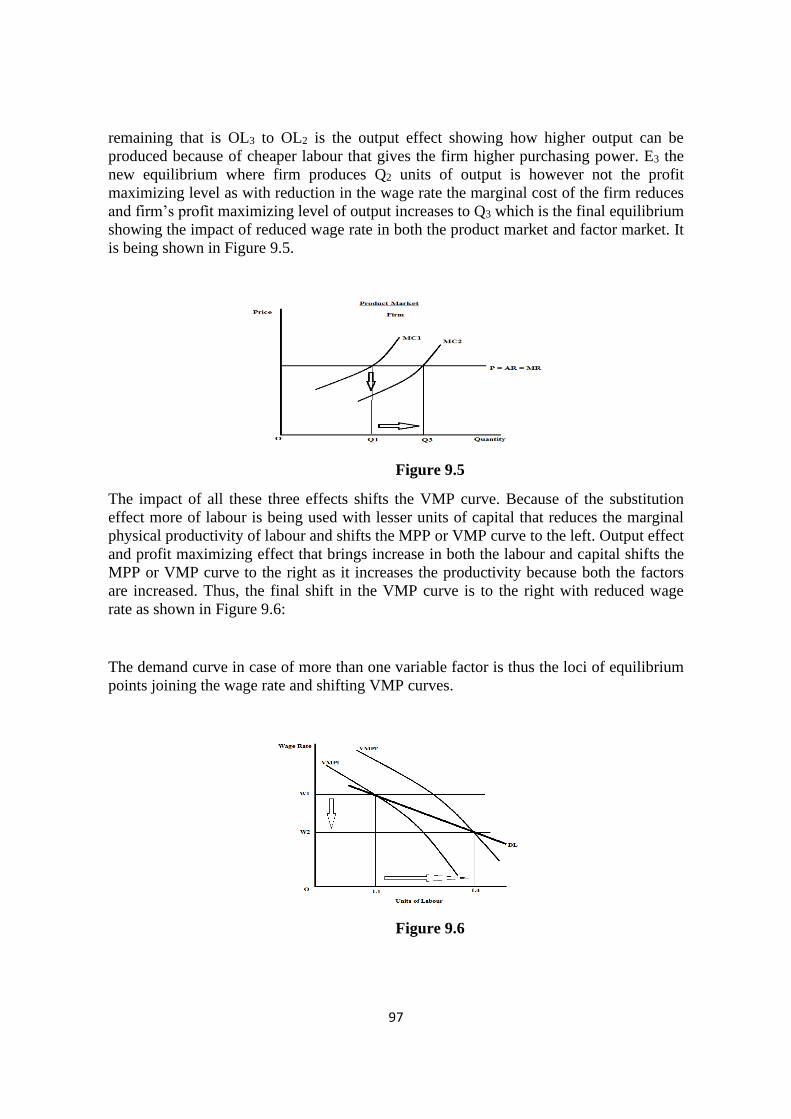
97

remaining that is OL3 to OL2 is the output effect showing how higher output can be

produced because of cheaper labour that gives the firm higher purchasing power. E3 the

new equilibrium where firm produces Q2 units of output is however not the profit

maximizing level as with reduction in the wage rate the marginal cost of the firm reduces

and firm’s profit maximizing level of output increases to Q3 which is the final equilibrium

showing the impact of reduced wage rate in both the product market and factor market. It

is being shown in Figure 9.5.

Figure 9.5

The impact of all these three effects shifts the VMP curve. Because of the substitution

effect more of labour is being used with lesser units of capital that reduces the marginal

physical productivity of labour and shifts the MPP or VMP curve to the left. Output effect

and profit maximizing effect that brings increase in both the labour and capital shifts the

MPP or VMP curve to the right as it increases the productivity because both the factors

are increased. Thus, the final shift in the VMP curve is to the right with reduced wage

rate as shown in Figure 9.6:

The demand curve in case of more than one variable factor is thus the loci of equilibrium

points joining the wage rate and shifting VMP curves.

Figure 9.6

98

Step 2: Demand for Factor of Production by the Industry

All similar firms when combined together form the industry. In the product market

horizontal summation of the demand of all firms is equal to the demand of the industry

but the same is not the case in factor market. It can be explained using Figure 9.7:

Figure 9.7

Initially with wage rate OW1, firm is using OL1 units of labour and if we assume that

there are n firms in the industry then the total demand of labour is horizontal summation

of the demand of labour by all the firms that is n*OL1. If wage rate reduces to OW2 then

all firms demand more of labour and produce more of the commodity. With increased

supply the price of the commodity in the product market reduces which shifts the VMP

curve to the left and hence at reduced price the demand of labour is OL2’ and not OL2.

Thus,cs demand for the whole industry is n*OL2’. So we see that in factor market the

demand of the industry is not simply the horizontal summation as is the case in the

product market because of interaction between factor market and product market.

Step 3: Supply of a Variable Factor of Production by a Single Individual

Supply of labour by one individual is backward bending showing that initially with

increased wage rate the individual supplies more of labour but with further increase in the

wage rate the individual substitutes leisure for work and reduces the supply of labour to

enjoy the wage that he has earned. It is explained with the help of indifference curve

analysis.

Figure 9.8

99

Figure 9.8 has leisure hours on X axis measured from left to right and hours worked from

right to left, and money income on Y axis. When wage rate is W1 the income– leisure line

is AM1 and individual is at equilibrium e1 where IC1 is tangent to AM1 where he is

having OL1 leisure hours and working for AL1 hours. Now if wage rate increases then

income– leisure line pivots to AM2 where individual moves to new equilibrium at e2

working for more number of hours that is AL2 to earn higher income. With further

increase in wage rates individual moves further to e3 where he reduces hours worked and

increases leisure hours to OL3. Joining the successive equilibrium points we get the wage

offer curve which shows that initially with increase in wage rate individual works more to

earn higher income and with further increase in the wage rate consumer reduces hours

worked to enjoy the income that he has earned. Above Figure can also be presented as

Figure 9.9.

Figure 9.9

thus, the supply curve of labour by an individual is backward bending as initially Income

effect is stronger that forces the individual to work more and earn higher income. with

further increase in wage rate substitution effect becomes stronger that forces the

individual to work less and substitute leisure for work.

Step 4: Market Supply curve of a Factor of Production (Labour)

The individual supply curve of labour is backward bending but for the market as a whole

the supply curve (Figure 9.10) is upward sloping because of the following reasons:

1. Geographical Mobility – With increased wage rate labour may move from

location to another thereby increasing the supply with increase in the wage rate.

2. Occupational Mobility – Individuals may also shift from one occupation to

another with increase in the wage rate thereby increasing the supply.

3. Retired individuals may also join the work force with increased wage rate.

4. Youngsters too join the work force as part time etc. with increase in the wage rate.

100

Figure 9.10

Step 5: Determination of Equilibrium Factor Price

As in the product market the price of the commodity is determined by the intersection of

market (industry) demand and supply curve, similarly the factor price too is determined

by the intersection of the industry demand and supply curve of the factor of production.

Taking the case of labour the equilibrium wage rate is determined in the following

manner (Figure 9.11):

Figure 9.11

The market demand for labour which is obtained from step 2 above is downward sloping.

The market supply curve of labour obtained from step 4 above is upward sloping. The

intersection of these two curves gives the equilibrium factor price (wage rate in this case)

which is OW* and OL* units of labour would be demanded and supplied.

Thus, marginal productivity theory explained how the pricing of factors of production is

done in factor market and how it is different from the pricing of commodities in the

product market. However, the theory suffers from various limitations which are given

below

Limitations of the Marginal Productivity Theory

1. Different units of factors of production are not homogeneous- The theory

assumed that all units of a particular factor of production are same in efficiency,

however this assumption is not always true for instance a labour may be more

efficient in working than some other labour and vice versa.

2. Factors of production cannot be easily substituted for each other- The theory

is based on the premise that two factors of production can be easily substituted for

each other to carry on the production such that if labour is not available then

101

capital can be substituted for labour to carry on the production, however this is not

always the case as production of a particular commodity requires a particular

proportion of different factors of production.

3. Criticism by Keynes- Economist Keynes criticized the marginal productivity

theory. The theory stated that if employment has to be increased then wages must

be lowered as it would attract more labour, however this can be true for a firm or a

particular industry but it is not applicable to the entire economy as it is the

aggregate demand that determine the level of employment in an economy and not

only the wages.

4. Assumption of perfect competition- Marginal Productivity theory assumed

perfect competition in both the product market and factor market. However this

assumption in itself is faulty as there is usually presence of imperfect competition

in the markets, so the theory needs modification to incorporate the imperfections.

5. Difficulty in measuring productivity -The foundation of the theory lies in the

productivity which in itself is difficult to measure as it assumes all the other

factors to be constant except the efficiency which however is not true. Efficiency

is in fact dependent on various factors simultaneously.


Check your progress


(a) Demand for factors of production is Direct demand.

(b) Factors of Production are always jointly demanded.

(c) Marginal Physical Product refers to addition made to total output by employing one

additional factor of production.

(d) Marginal Productivity theory assumes perfect competition in both product and factor

markets.

Ans. 1(F), 2(T), 3(T), 4(T)


(a) Marginal Physical Productivity theory was given by _ _ _ _ _ _ _ _ .

(b) In case of perfect competition in product and factor market the value of marginal

revenue product and value of marginal product is _ _ _ _ _ _ _ .

(c) The price of a factor production is dependent on its _ _ _ _ _ _ _ _ _ _ .

Ans 1. Clark 2.same 3. productivity


1. Explain the different concepts of Productivity.

2. What are the assumptions on which Marginal Productivity Theory is based?

102

3. How Marginal Revenue Product is different in case of Perfect competition and

imperfect Competition in the product market. Explain using an example.

4. How the prices of factors of production are determined using Marginal Productivity

Theory?

9.5 ECONOMIC RENT

The concept of Economic rent was first given by David Ricardo (1772– 1823 “Rent is

that portion of the produce of earth which is paid to landlord for the use of original and

indestructible powers of the soil.”

Ricardo gave two reasons for the existence of rent:

1. Scarcity of resources and

2. Alternative use of the resources.

Modern Economists like Joan Robinson etc. however were of the opinion that rent is not

only attributable to land but any and every factor of production can earn rent, whereby it

is defined as the excess of actual earnings over the amount that is needed to keep the

factor of production in its present use, the latter being termed as transfer earning. To

understand the concept of Economic rent the concept of transfer earnings needs to be

understood. It is the minimum amount that is to be paid to a factor of production to

prevent it from moving to an alternative. Example: If a worker is being paid Rs 2000 per

day for working as an executive whereas for working as an officer he would have been

paid Rs 1500, thus Rs 1500 is the transfer earnings. Thus, rent in this case can be

calculated as:

Economic Rent = Actual Earnings – Transfer Earnings

= Rs 2000 – Rs 1500

= Rs 500

The amount of economic rent depends upon the elasticity of supply of the factor of

production such that there can be following three cases:

1. Perfectly Inelastic Supply – If a factor of production is perfectly inelastic then its

transfer earnings are zero as it has no opportunity cost or alternative use, thus

whatever the factor earns it is all economic rent. It is shown in Figure 13:

Such a situation is usually found in case of specialists like singers, professionals etc.

who earn all the rent in the form of economic surplus.

2. Perfectly Elastic Supply – When a factor of production is perfectly elastic then it

can be easily shifted to its alternative and hence whatever it earns is the transfer

earning and it is equal to actual earnings and hence economic rent is zero Figure

14. It takes place in case of unskilled labourer, rickshaw pullers etc.

103

3. Relatively Inelastic Supply – When the supply is relatively inelastic then a part

of actual earning is paid to prevent its transfer to the alternative use and the

remaining that is in excess is the economic rent. Thus, here actual earnings are

more than the transfer earnings as is shown Figure 15:

Figure 13 Figure 14 Figure 15

The size of economic rent received by a owner of a factor of production is determined by

the elasticity of supply for that particular good or service.

(a) If the elasticity of supply is neither elastic nor inelastic, the supply curve will slope

upward, and the supplier's income would be split between economic rent and opportunity

cost.

(b) If the elasticity of supply is inelastic, the supply curve would be perfectly vertical, and

the supplier's entire income would be comprised of economic rent. For example, if the

supply were a particular plot of land, or a

(c) If the elasticity of supply is elastic, the supply curve would be perfectly horizontal,

and the supplier's entire income would be comprised of opportunity cost.


Check your progress


(a) Marginal Physical Product refers to addition made to total output by employing

one additional factor of production.

(b) Economic Rent arises only to land.

Ans. A. (T), b. (F)


(a) Economic rent concept arises because of ……………… of resources.

(b) In case of monopoly in product market and perfect competition in the factor

market the ……………… curve is used.

(c) The price of a factor production is dependent on its ……………… .

Ans 1. Scarcity 2.MRP 3. Productivity

104



Factor Price determination is not as simple as commodity pricing as apart from demand

and supply there are various other factors that have an impact on the prices that the

factors of production command in the market. Moreover, there is an interaction between

the product market and factor market that determines the demand of any factor of

production as factor’s demand is indirect or derived from the demand of the commodity

that it produces. Also, the demand for factors of production being joint demand the

prices, availability, efficiency and substitutability of other factors of production also

impact the prices of a particular factor of production. Various economists have given

various theories to determine the factor prices the most prevalent is the Clark’s Marginal

productivity theory that assumes perfect competition in both the product market and

factor market and based on various other assumptions determine that the price of a

variable factor of production is determined by the intersection of the market demand and

market supply of that factor.

The concept of economic rent as given by traditional economists and modern economists

too had been explained where rent is defined as the excess of actual earnings over the

transfer earnings and can be earned by any and all factor of production whose supply is

not perfectly elastic.


1. Explain the concept of economic rent. How does elasticity of supply of factor

affect economic rent?

2. Critically examine the marginal productivity theory of factor pricing?

3. What is the reason behind supply of labour to be backward bending? Explain by

using suitable diagram?

105

LESSON 10

INTERNATIONAL TRADE

Anirudh

Laxmibai College, University of Delhi

10.1 INTRODUCTION

The term trade refers to exchange of goods and services and when it takes place across

the countries, it is called international trade. All countries are not sufficient in themselves.

Different countries different endowed with resources, Generally, while a country has the

abundances or surplus of some resources it suffers the scarcity of certain others.

Gulf countries for example are endowed with expensive oil beyond what they

themselves would need. But therefore suffering the scarcity of industrial goods and food

grains. In such; situations, trade across the boundaries helps to exchange your surplus

goods with those who do not have. International trade implies international specialization.

An economy that engages in international trade is an open economy. A country that

does not involve in trade is called closed economy and situation in which a country

conducts no foreign trade is called autarky. The advantages which are gained from trade

with other country fare called the gains from trade.


After going through this lesson, you will be able to

• Explain International trade or specialization

• Understand basis of trade

• Differentiate between regional and international trade

• Explain as to why do nations trade

• Know gains from trade

• Learn the theories of absolute and comparative advantage

• Understand the scope of study of international trade

10.3 DISTINGUISH BETWEEN INTERPERSONAL, INTERREGIONAL AND

INTERNATIONAL TRADE

Each person would have to be self-sufficient without trade. If the person would produce

all the food, clothing, shelter, medical services, entertainment and luxuries etc. But it is

impossible for the particular person, Therefore, trade between individual allows people to

specialize in those activities of which they can do relatively well and to buy from others

the goods and services at which cannot be produced by them easily. It is called

interpersonal trade.

106

International trade is also based on interpersonal trade. Each region would be forced

to be self-sufficient. If trade does not exist between these regions. But trade exist in the

region where each region can special in producing those goods or services for which it

has some natural resources plain regions can produce that specialized goods which their

abundance in that natural resources. For example, plain areas can produce different food

grains while mountains regions can specialize in mining and forest products.

Therefore, each region showed produce that goods in which it has some natural

resources or acquired advantage and obtains other products of trade when all region scale

to self-sufficient.

The interpersonal and interregional principles which have been mentioned in the

case the nations, the international trade arises. Almost all countries produce more of some

goods than their residents wish to consume. At the same time, they consume more than of

that commodities whatever are producing.

International trade is necessary to achieve the gains that international specialization

makes possible. Trade allows each individual region or nation to concentrate on

producing those goods and services that it produces relatively efficient while trading to

obtain goods and services that it would produce less efficiently than others.

10.4 INTERNATIONAL TRADE IMPLIES INTERNATIONAL SPECIALIZATION

From the individual’s point of view, specialization refers to the acquisition of a

specialized skill in the performance of particular activity or in the production of a

particular commodity. From the country’s point of view, it refers to utilization of the

country’s resources, in specialized areas of production in which the country has absolute

or comparative cost advantage compared to the rest of the world. When the country’s

resources are utilized in certain specialized areas, production of specialized commodity

tends to be more than their domestic need. The surplus products are exposed.

On the other hand, when resources are withdrawn from the non-specialized areas

production of certain commodities falls short of the country’s domestic requirements.

This refers import situation. International trade-exports and imports are the obvious

outcome of international specialization. Since international specialization is based on the

principle of some theory which were given by different economists, the significance of

international specialization lies in gains from trade.

Determinants of International Trade

There are different factors which affect the international trade or international

specialization which follows:

1. Natural Endowment – Natural endowment is the basic of international

specialization. It refers to the resource base of a country available to it as a free

gift of nature. Natural endowment also includes nature and fertility at the soil as

well as climate conditions. Thus, India and Srilanka specialize in the production

of tea simply because of the conducive climatic conditions.

107

2. Technical condition – International specialization also depends upon technical

conditions of the country with their technical advancement developed of the

world have solved all ^confronts of natural endowment. Japan, for example, is

just a small coastal country which has a few natural resources, but its technical

superiority had made the distinction of most advanced nation in their field of

Automobile production.

3. Lost differences – The fundamental basis of international specialization is the

difference between the cost of production of the different commodities. Different

countries specialize, in the production of those goods in which they have absolute

or comparative cost advantage. The important parameter of competitiveness in

the international market is the cost different of the produced goods.

4. New Economic order: Globalization of the World market through multi-

national corporative and the emergence of new economic order has forced

various nations to integrate their economies with the rest of the world, leading to

greater degree of specialization and international trade.

10.5 ADVANTATE OF INTERNATIONAL SPECIALIZATION OR

INTERNATIONAL TRADE

There are different advantages from international trade or specialization which follows:

1. Fuller utilization of Natural Resources – International trade enables the natural

resources to be exploited fully. Underdeveloped countries are not in a position to

utilize natural resource fully. Such countries export their raw materials to

developed industrial countries.

2. Cheaper goods – International trade provides cheaper goods to those countries

which cannot produce the particular goods. It is so because every country

produces those goods in the production of which it has to incur less comparative

cost. Accordingly, international specialization or trade facilitates higher level of

consumption and therefore better quality of life.

3. Surplus production – International specialization enables every country to

dispose off its surplus production. Some countries produce more goods than their

own requirement. They sell this surplus production in other countries and they

avoid the occurrences of deflationary pressures in the domestic economy.

4. Bulk production and economies of scale – On account of international

specialization, ‘different countries specialize in the production of those goods

alone in which they enjoy favorable production conditions. As a result goods are

produced in large quantity at low price in consonance with the economics of scale

in the words of Mconnell, "International trade is a means by which nations can

specialize increase the productivity of their resources and thereby realize a larger

output than otherwise.

5. Possibility of Economic Development – Economic development of any

countries depends upon the international trade. Underdeveloped countries can

make the optimum use of their available natural resources and raw materials by

108

imparting machinery and technical equipment from, the developed countries.

They are thus enabled to increase their output and exports and thereby promote

economic development. In the words of Robertson, "International trade is an

engine of growth".

6. International co-operation – Mutual co-operation can be developed on the basis

of international specialization with the different countries. It creates an

atmosphere of good will, cordiality and friendship among the trading countries.

According to Henry Cornez, "International specialization is the greatest civilizing

agency.

10.6 THE GAINS FROM TRADE OR SPECIALIZATION WITH GIVEN COSTS

The gains from trade depend on different theory is which some are discussed below:

According to this theory difference is cost of production of different goods across

different nation constitutes the fundamental basis of international trade. Here, we will

discuss absolute advantage and comparative advantage theories respectively.

1. Absolute Advantage

Adam Smith gave absolute differences cost theory. According to this theory, absolute

difference in the cost of production of different goods across different counties is the

basic reason behind the international specialization trade. The absolute cost difference

arises when one country is in a position to produce a commodity at a very low cost

compared to another country and the other country can produce some other commodity of

a very low cost compared to the first country. All there becomes possible when a country

is endowed with a special kind of soil, climate conditions and facilities. Consequently, a

country specializes in the production of a particular commodity and exports it to other

countries and imports another commodity from another country in which the letter

specializes. It is further elaborated with the help of table 10.1.

TABLE 10. 1

Absolute Difference in costs production of two countries

Countries Rice Wheat

India 2 4

Nepal 4 2

Total 6 6

It is clear from above table 10.1 that one unit of labour produces 2 units of rice or 4

units of wheat in India, on the other hand one unit of labour in Nepal produces 4 units of

rice and 2 units of wheat. It is clear that

In India 1 unit of rice = 2 units of wheat

In Nepal I unit of rice = 0.5 units of wheat

109

It is quite clear from the above example that India has an absolute advantage in the

production of wheat and Nepal in production of rice. It is an essential condition of

interference Trade that the production cost in two trading countries should be different.

The cost of the rice for wheat in India is 1 : 2 and in Nepal it is 1 : 5 there is no trade

between those two countries and both produce both the commodity then two days of

labour will produce in the two countries total of 6 unites of wheat and 6 units of rice.

Suppose India specializes in wheat and Nepal in rice and they trade with each other. This

can be shown by diagrammatically:

Figure 10.1

In the above figure 10.1, AB curve is the production possibility curve of Nepal and

AC curve is the production possibility curve of India. Production possibility curve states

that with the help of a given quantity of factors of production in order to produce more

unit of a commodity how many units of another commodity will have to be sacrificed.

Slope of these curves indicates the opportunity cost to two commodities opportunity cost

also means that in order to produce one more unit of a given commodity how many units

of another commodity are to be sacrificed. This figure is based on the assumption of the

law of constant costs. That is why production possibility curves are straight lines/ AB

curves states that if Nepal is to produce one unit of rice, it will have to sacrifice 0.5 unit

of wheat. Hence if by giving one unit of rice it gets more than 0.5 unit of wheat, it will be

a gainer. Similarly, AC curve indicates that if India chooses to produce one unit of rice it

will have to sacrifice two units of wheat if, however, India gets one unit of rice by

parking with less than two units of wheat then India will stand to gain by producing what

shaded area ABC in the above figure refers to the gain from international trade.

Distribution of this gain between the two countries will depend upon the terms of trade.

Terms of trade are governed by the reciprocal demand of the countries concerned for each

other’s product.

2. Theory of Comparative Costs

Theory of comparative costs was discussed by the famous economist David Ricardo in

his book principles of political economy and taxation. The theory is also called theory of

comparative advantage. Ricardo theory of comparative costs claims that trade enables

110

countries to specialize in producing the products that they produce best. According the

theory, specialization and free trade will benefit all trading partners even those that may

be absolutely loss efficient producers.

Ricardo’s comparative cost theory is based on the following assumptions:

1. There are only two countries and they produce two goods

2. Labour is the only factor of production and cost of production is measured in

terms of labour units

3. All units of labour are homogenous

4. Production is subject to law of constant returns

5. Factors of production are perfectly mobile within the country but are perfectly

immobile between two countries

6. There is no cost of transportation

7. International trade is free from all government comforts

8. There is full employment in countries engaged in international trade

9. There is perfect competition both in the goods market and factor market.

Comparative Difference in Costs

The comparative difference in the costs was given by David Ricardo. According to him,

comparative difference in cost is the safe cause of international trade. Comparative

difference in costs means that a country is in a position to produce both the goods at

absolutely less cost than the other country. Yet it has greater comparative advantage in

the production of one of the two goods, while it has less comparative advantage in the

production of the other good. The other country produces both the goods at a higher cost,

but it has less comparative disadvantage in the production of one goods, while it has

greater comparative disadvantage in the production of the other good.

Comparative advantage refers to the advantage in the production of a product by one

country over another when that product can be produced at lower cost than in the other

country in terms of other goods.

For example, there is a leading practicing lawyer in Delhi who is also a proficient

typist. His clerk also knows typing but nothing about legal practice. Although the said

lawyer is competent in both the jobs, yet he will gain comparatively more if he denotes

all his time to legal practice. On the other hand, the clerk is less capable than the lawyer,

still in typing job his comparative disadvantage is least. If the lawyer confines himself to

legal practice and entrusts the typing job to his clerk, he will enjoy greater comparative

advantage.

In short, a country may have absolute cost advantage in the production of both goods

A and B. Yet it may opt to specialize in A rather than B, because A offers comparatively

greater cost advantage than B.

This can be shown by Table 10.2

111

TABLE 10.2

Wheat Clothes

(Metre)

India 0.60m cloth 1.67 kg wheat

Nepal 2.00m cloth 0.50 kg wheat

We assume that the opportunity cost of producing 1 kilogram of wheat is 0.60 meter

of cloth in India, while in Nepal it is 2 meters of cloth. The second column of this table

gives the same information again but expressed as the opportunity cost of 1 meter of

cloth. India has a comparative advantage in wheat production and Nepal is in the cloth.

It can be seen diagrammatically

Figure 10.2

AB is in the production possibility curve of India and AC of Nepal. It means that to

get one meter of cloth, India has to sacrifice one unit of wheat. Nepal can get two units of

wheat, by sacrificing one meter of cloth. It is clear that India has greater comparative

advantage in the production of cloth and Nepal has least comparative disadvantage in the

production of wheat.

By giving one unit of cloth to Nepal, India can get in exchange more than one unit of

wheat. On the other hand, by with less than 2 units of wheat. Nepal can get one meter of

cloth from India. Advantage arising out of international trade to both the countries is

shown by the shaded area A advantage will be distributed between the two countries on

the basis of settled terms of trade. Terms of trade are settled on the basis of reciprocal

demand for each other’s product.

Criticism of the Theory

Ricardo’s theory of comparative costs is an important theory of international trade. In the

words of Samuelson, "The theory of comparative advantage has in it a most important

glimpse of truth". Despite being reciprocal from the logical point of view, it has many

shortcomings.

112

1. Only a Normative Theory – Ricardo’s theory of comparative costs is only a

normative theory. It does explain as to how the resources of the country can be

put to optimum use, but it fails to explain the composition of international trade

or the nature of exports and imports and what are their problems. It is not a

positive explanation of international trade.

2. Based on labour Theory of value –Theory of comparative costs is based on the

theory of labour cost. According to this theory, cost of a good depends upon the

amount of labour necessary to produce it. But in reality, cost of a good is also

influenced by the price of other factors like land, capital etc. in addition to that of

labour. Critics of this theory therefore like to examine it in terms of money cost

in place of labour cost.

3. Transport costs ignored – One of the main defects of the theory of comparative

costs is that it does not take into account transport cost. In case of some

commodities transport costs are higher than their production costs. It is therefore

essential that while exporting and importing of goods total costs should be

calculated by taking into account both production and transport costs.

International trade is very much influenced by transport costs. It cannot be

ignored.

4. Based on the low of constant costs – The theory assumes that cost of production

per unit remains constant even if production is increased or decreased. The

assumption is not only unrealistic but unscientific also. Ordinarily one finds that

production is subject to the law of increasing costs or law of diminishing costs.

The possibility of the opinion of law of constant costs is rare.

5. Impossibility of complete specialization – It is not possible for the countries

participating in international trade to specialize fully in the production of some

goods supposing India and Nepal enter into international trade India specialists in

the production of cotton cloth and Nepal in the production of woolen cloth. Nepal

being a small country cannot meet fully the demand of India for woolen cloth nor

can it absorb all the cotton cloth produced in and exported from India. Hence we

will have to produce both cotton and woolen cloth, It can therefore be asserted

that full-scale international trade is possible only when it is between two equi-

sized countries producing goods at equal value.

6. Based on the free trade – Classical economists assume that international trade is

free from all restrictions, but the situation in the modern times is entirely

different. No country wishes to expand upon any other country to the extent that

it is pushed into the realm of uncertainties. Besides, several other situations like

imperfect competition, trade restrictions, state trading, export-import duties and

economic planning do not allow complete freedom of international trade.

7. Static Conditions – Another assumption implied in this theory is that tastes of

the people and production conditions in two countries remain unchanged. Besides

the supply of land capital and labour remain static. But in real world all these

things go on changing from time to time. This assumption therefore is baseless.

113

8. One-sided – Ricardo’s theory of international trade is one-sided. It takes into

account the supply side of the trade but ignores the demand side. It tells us what

goods a country imports or exports but does not explain as to how terms of trade

and rate of exchange are determined.



1. International trade takes place due to natural endowment, absolute and

comparative difference in costs etc.

2. International trade leads to specialization in production, fuller utilization of

resources, improvement in economic relations between countries and economic

development etc.


1. Explain the theory of comparative cost advantage in the context of

International Trade.

2. Distinguish between absolute and comparative advantage and show how

all trading nations could gain from trade.

114

LESSON 11

TERMS OF TRADE, FREE TRADE AND PROTECTION

11.1 LEARNING OBJECTIVE

After going through this lesson, you will be able to

1. Know the meaning and formula of terms of trade

2. Understand the concept and advantages of free trade

3. Know the case and methods of protection

11.2 TERMS OF TRADE

The terms of trade refer to the rate of which the goods of one country are exchanged for

the goods of another county. It is a measure of the purchasing power of exports of a

country in terms of in its imports and is expressed as the relation between exports prices

and imports prices of its goods when the export prices of a country rise relatively to its

import prices, its terms of trade are said to have improved. On the other hand, when its

import prices rise relatively to its export prices, its terms of trade are said to have

deteriorated. In case terms of trade deteriorate for a country its gain from trade is reduced

because now it can have a smaller quantity of imports in exchange for a given quantity of

exports than before.

Terms of trade refer to the physical exchange ratio at which goods are exchanged for

one another between the countries when trade takes place between two open economies

certain goods are affected for sale by both the countries. Since many commodities are

exported and imported simultaneously from both the sides, we can no longer use the

physical quantities like in terms of kilogram of wheat or meters of cloth. We find the

index of export prices and index of import prices to determine the terms of trade.

We use the following formula to estimate terms of trade:

Terms of trade = Index of export prices

100Index of import prices

This is also called the index of terms of trade. Terms of trade become favourable for

a country if this index increases. Suppose export prices increase by 15% (i.e., price index

of export increases from 100 to 115) and import prices increase by 5% (i.e., price index

of import increases from 100 to 105), then the index of terms of trade increases from 100

to 109 (115/105 × 100 = 109). That is at new terms of trade one unit of exports will buy

5% more imports than at the old terms.

Similarly, term of trade becomes unfavourable when percentage change in export

prices is less than the percentage change in import prices. In such situations terms of trade

index is below 100. Suppose export price index increases by 5% and import price index

increases by 10% then the terms of trade index should be

Terms of trade (TOT) = 105/110 × 100

115

In this case one unit of export will buy approx. 5% less imports.

Terms of trade are closely related to competitiveness. If the is 9, substantial increase

in export prices implying a significant increase in index of term of trade, it may in fact be

a situation of loss of competitiveness.

Question: What do you understand by terms of trade?

11.3 MEANING OF FREE TRADE

A trade policy which does not impose any barrier on the exchange of goods and services

between different countries, is know as the free trade policy. Free trade allows all

countries to specialize in producing products in which they have a comparative

advantage, According to Smith, the concept of free trade policy refers to a system of

commercial policy which draws no distinction between domestic and foreign

commodities and thus which neither imposes additional burden on the letter nor grants by

special favour to the farmer. Thus, free trade policy permits international flow of goods

and services without any artificial impediments. Hence a world of free trade would be

one with no tariffs and no restrictions of any kind on importing or exporting. In such a

world a country would import all those commodities that it would buy from abroad at a

delivered price lower than the cost of producing then at home.

Advantages of Free Trade

There are different advantages of free trade policy which are follows:

1. Maximization of output: According to the principle of comparative cost

advantage every country would specialize in the production of that commodity

for which it is best suited or in the production of which it had comparatively

greater advantage. This would create the maximization of wised output of diverse

goods and services.

2. Optimum utilization of resources: Since production is conducted on the principle

of Comparative cost advantage then the resources are optimally utilizes. Each

country produces goods with least cost combination of inputs.

Disadvantages of Free Trade

The policy of free trade came to be practically abandoned after the great depression both

on theoretical and practical grounds of which the following are the important ones:

1. Free trade pre-supposed the existence of laissez faire and the working of price

mechanism under perfect competition. But these conditions do not exist in the

present-day world. Monopoly, monophony, carrels imperfect labour markets and

tariffs led to the abandonment of the free trade.

2. Under the policy of free trade, some industries possess comparative advantage,

but other industries are not developed so this naturally leads to the one-sided

development of the economy.

3. As under the regime of free trade there was laissez faire policy and the state did

not impose any restrictions on the international movements of goods among

116

nations. Many harmful commodities ‘came to be imposed by unscrupulous

merchants in a number of countries. This had extremely harmful effects on the

health and welfare of the country.

4. Free trade policy may lead to the emergence of international monopolies and

local monopolies. According to Haberler such monopolies developed under free

trade which proved harmful to the other countries and the domestic interests. This

factor also led to the adoption of the policy of production.

5. Prof Haberler view that policy of free trade would help rapid economic

development of backward countries cannot be accepted It is now well recognized

that underdeveloped countries can develop better under a policy of protection

rather tax-free trade.

Question: What is commercial policy and explain the advantages and disadvantages

of free trade.

11.4 THE CASE FOR PROTECTION

The term protection refers to a policy whereby domestic industries are to be protected

from foreign competitions. The aim is to impose restrictions on the imports of low-priced

production in order to encourage domestic industries productions high price products.

The domestic industries may be protected by imposing import duties which raise the price

of foreign goods by more than the price of domestic goods or they may be protected by

groups of other non-tariff restriction which make imports of cheap foreign goods difficult

or impossible or the domestic industries may be paid subsidies or aunties to enable them

to compete with cheap foreign goods. There are two kinds of argument for protection

which are commonly offered 1. Economic Arguments and 2. Non-Economic Arguments

Economic Arguments

The economic arguments usually offered in favour of protection. There are important

arguments for the use of tariffs when the objective to make national income as large as

possible.

1. To protect infant industries

To protect infant industry was first of all formulated of Alexander Hamilton but was

popularized by F List. The aim of protection is to raise the standard of living in the

country. It comes in a state and dynamic form. The static form assumes that world

technology is given and constant. If an industry has large economies of scale costs will be

high when industry is small but will fall as the industry grows. It is argued that if

industries in their infancy are not protected from established foreign producers, they

cannot develop to enjoy the comparative advantages. So, they are protected by providing

all types of facilities such as subsidies heavy import duties on foreign goods etc. They

may expand and enjoy internal economies of scale.

A newly developing country may find that in the early stages development its

industries are unable to compete with established foreign rivals. A trade restriction may

protect these industries from foreign competition while they grow up If these industries

117

would be in the developed condition then they will be able to produce as cheaply as

foreign rivals and therefore will be able to compete without protection.

The dynamic form of the argument emphasizes that technology is constantly

increasing endogenously. Those industries which were stagnant in the early stage of

development will gain technological experience and advancement. A country needs to

protect its domestic industries during the early stages of development when industries are

using the technology. The objective is not to move along a given falling long run cost

curve but rather to develop industries that will have cost curves that fall over time as fast

as the similar cost curves are falling in the advanced countries because of invention and

innovation. To prevent the new industries from becoming stagnant under the protection

that shields them from foreign competition the protection must be consistent on achieving

success in foreign markets within a stated period of time. Once they have developed the

skills needed to hold their own in the intense international competition associated with

new technologies then protection can be removed. The advocates of their arguments for

early protection point out that all the economically advanced countries developed their

early industries under tariff protection:

2. To encourage learning by doing:

The dynamic version of the infant industry argument is supposed by the argument

based on learning by doing learning by doing suggests that the pattern of comparative

advantage can be changed. If a country learner enough through producing product in

which it currently is at 9 comparative disadvantages, it may gain in the long run by

specializing in those products and could develop a comparative advantage as the learning

process lowers their cots.

Protecting a domestic industry from foreign competition may give its management

time to learn to be efficient and its labour force time to acquire the needed skills.

Some countries have, succeeded in developing strong comparative advantages in

targeted industries but other may failed. One reason such policies sometimes fail is that

the industries and complacent. Another reason is the different of identifying the industries

that will be able to succeed in the long run.

3. To create or to exploit a strategic trade advantage

An important recent argument for tariffs or other trade restriction is the need to

create a strategic advantage in producing or marketing. New product will be expected to

increase the normal profits. Some goods are produced in industries containing barrier to

further entry. Firms in those industries can earn extra high profits ever long periods of

time. Where such industries are already well established then is little chance that a new

firm will replace one of the existing grants.

The first firm to develop and market a new product successfully may earn

substantial pure profits over all of its opportunity costs and become one of the few

established firms in the industry. If protection of the domestic market can increase the

chance that one of the protected domestic firms will become one of the established firms

in the international market the protection may pay off.

118

There are lots of high-tech industries which are facing declining average total cost

because of their large fixed cost of product development. For example, a new generation

of civilian aircraft, computers software and pharmaceuticals. They are fixed costs of

entering the market. They must be increased before a single unit of output can be sold in

such industries a few firms can find place.

The characteristics just described are sometimes used to provide arguments for

subsidizing the development of such industries or protecting their home market with a

tariff. Suppose for example that there is room in the aircraft industry for only three major

producers of the next round of passenger jets. If a government assists a domestic firm,

this firm may become one of the three that succeed and the profits that are subsequently

earned many more than repay the cost at the subsidy.

On the basis of above discussion, the economists advise that their governments

should adopt strategic trade policies more broadly than they now do. This means for high-

tech industries, government protection of the home market and government subsidization

of the product development stage.

Criticism: Critics argue that one all countries try to be strategic. They will all waste

vest sums trying to break into industries in which there is no room for most of them.

Supposes of strategic trade policy reply that a country cannot afford to stand by white

others play the strategic game. According to advocates who support the strategic trade

policy that there are key industries that have major spillovers into the rest of the

economy. If a country wants to have a high standard of living it must compete with the

best if a country lets all of its key industries migrate to other countries many of the others

will follow. The country then risks being reduced to the status of a less developed nation.

Opponents argue that strategic trade policy is just the modern version of

modernization, a policy of trying to enrich oneself at the expense of neighbors rather than

working for mutually beneficial gains from trade. There are real doubts that such

prosperity could be maintained if the volume of trade were to shrink steadily because of

growing trade barriers.

To Protect Against Unfair Actions by Foreign firms and Governments

Tariffs may be used to prevent foreign industries from gaining an advantage over

domestic industries by using practices that will harm domestic industries and hence lower

national income. Subsidies and dumping are used to protect against unfair actions by

foreign firms and government.

To Alter the Terms of Trade

Trade restrictions can be used to turn the terms of trade in favour of countries that

produce and export a large of the world’s supply of some product. They can also be used

to turn the terms of trade in favour of countries that constitute a large fraction of the

world demand for some product that they import.

Suppose a country that provides a large fraction of the total demand for some

product that it imports.

119

But restrictions are imposed on the demand for the commodities through tariffs, it

can force the price of that product. This turns the term of trade in its favour because it can

now get more units of imports per unit of exports.

Non-Economic Argument

There are important non-economic arguments favouring protection. These factors are not

maximizing rational income.

1. Defence Argument – A country should adopt the policy of protecting its

industries from the standpoint of national defence. If a country is dependent on

the other countries for its requirements of agricultural and industrial products, it

will be very harmful for its national interest in terms of war.

2. Non-economic advantages of diversification – Comparative advantage might

dictate that a country should specialize in producing a narrow range of products.

The government might decide that there are distinct social advantages in

encouraging a more diverse economy. Citizens should be given a wider range of

occupations. The social and physiological advantages of diversification would

more than compensate for a reduction in living standard.

3. Risk of Specialization – The specialization in the production of only a few

products many involve risks that country does not wish to take. One such risk is

that technological advances may render its major product obsolete. The pro-tariff

argument is that the government can encourage a more diversified economy by

protecting industries that otherwise could not compete.

4. Protection of specific groups – Although free trade will maximize per capita

GDP over the whole economy, specific groups may have higher incomes under

protection than under free trade. If a firm or industry in a monopoly condition,

then tariffs are used to restrict foreign competition. Tariffs tend to raise the

relative income of a group of people who are in short supply domestically and to

lower the relative income of a group of people who are in plentiful supply

domestically tree trade does not the opposite.

Question: What do you understand by protection? Explain the economic and non-

economic arguments for protectionism.

11.5 METHODS OF PROTECTION

We have now studied some of the many reason why government may wish to provide

some protection for some of their domestic industries. Policy instruments of protection

are broadly classified as:

1. Tariff barrier 2. Non-tariff barriers

1. Tariff Barriers – Tariff which is imposed by different countries in the world has

been the most important type of trade restriction. A tariff is a ban or duty levied

on the traded commodity as it crosses a national boundary. An import tariff is a

duty on the imported commodity while an export tariff is a duty on the exported

commodity. In the context of the policy of protection import tariffs are more

120

important than export tariffs. Infact tariff barriers are basically concerned with

import duty. There are main two type of protection policy, first policies that

directly raise prices and second policies that directly lower quantities.

The first type of protectionist policy directly increases the price at imposed

commodities thereby offering protection to the domestic producers from international

competition. A tariff which is often called an import duty is the most common policy of

this type.

In case of restricted trade

It illustrates how gains/loss occurs to the consumer the government the domestic producer

and the foreign producer when the tariff is imposed.

Now, tariff given by it is imposed for each unit imported. Consequently, the price

increases of each domestic producer receive Pd price for all units sold.

After imposing tariff barriers, the domestic price is increased by amount of tariff

hence there is loss to domestic consumers and foreign producers and again to the

domestic producers of course the government gains in terms of tax revenue.

2. Non-tariff barriers – The second type of protectionist policy directly restricts

the quantity of an imported product. All the barriers that do not directly increase the price

of an imported commodity are called non-tariff barriers. In other worlds, any direct or

indirect trade restriction which does not involve tariff is called non-tariff barrier, import

quota is one of the important types of non-tariff barriers. Under import quotas, the

importing country sets a particular limit for a commodity beyond which no import is

allowed during the stipulated time period.

Apart from import quota, for may years there has been in operation the voluntary

export restriction (VER) through an agreement between the trading countries exporting

country to agrees to limit the amount of a good that it sells to the importing country.

Question: What are the methods of protection?

Question: Distinguish between tariff and non-tariff barriers.

Fallacious trade policy arguments

There are many fallacies that exist for free trade as well as for protectionism. We have

also seen that there are some valid arguments for a moderate degree of protectionism for

one specific country. Fallacious arguments are heard on both sides and they colour much

of the popular discussion. Such arguments have persisted for ages, but their survival does

not necessarily make them true. We examine them now to see where their fallacies lie.

(A) Fallacies related to free trade argument

1. Free trade always benefits fall countries – It is a standard knowledge that most

developed economies do not believe in free trade. Infact a small group of

developed countries tend to collude to make and after the terms of trade in their

favour by following restrictive trade policies. If they resort to free trade

unilaterally, they will lose the advantages earlier enjoyed under the tariff

121

protection regime. Thus, free trade does not necessarily maximize income or

benefit of every trading partner.

2. Infant industries never abandon their tariff protection – It is argued that

granting protection to infant industries is a mistake because these industries

selfdom admit to growing up and will cling to their protection even when fully

grown. But infant industry tariff is a permanent tariff protection would be

required to protect a weak industry never able to compete on an equal looking in

the international market. But if the industries do grow up and achieve the

expected scale and learning economies, the real costs of production are reduced,

and resources are freed for other uses

3. Free trade maximizes world income under real world conditions – Free trade

can be shown to maximize world income when technology and comparative cots

are given. But if technology is changing endogenously as a result of conscious

decisions taken by firms and other agents of charge it cannot be proved that

completely free markets will maximize income over time it is possible that some

types of government interventions or market imperfections will produce more

technological change than completely free and fully competitive markets.

(B) Fallacious arguments for protectionism

1. Avoid exploitation – According to this argument the free trade policies benefit a

nation at the cost of the other. In other words, free trade would never be mutually

advantage as one party always gains at the expense of the other. In such a

situation, it becomes necessary for weaker nations to protect themselves through

various protectionist policies like tariffs port quota etc. But, the principle of

comparative advantage refuses this argument by showing that both the trading

partners tend to gain from international trade provided opportunity cost refers

differ across the nations. Specialization and trader are expected to enhance

production and consumption.

2. Protects against low-wage foreign labour – It is often argued that in industrials

countries the cheap imports from low-wage nations will drive out domestic

products from the market. This would lower the standard of living in

industrialized nations down to the level prevailing in the low wage nations.

However, this argument is not completely true as the developed nations tend to

gain by obtaining imports at a low cost in exchange for the goods which must be

exported owning to their surplus domestic production mutually beneficial trade is

based on comparative advantage rather than the absolute advantage low-wage

nation specializing in the production and export of capital intense commodities.

Even if this does not happen high domestic labour costs can be effectively

lowered if productivity of labour is higher than in low wage countries of abroad.

Another side of the argument is that in the long run a richer nation can hurt itself

by importing cheaply and not exporting at all. But imports can only be obtained

by spending currency of that nation. And foreign currency can be obtained either

by exporting or by borrowing since one cannot borrow for long exports become

122

essential. Hence trade always moves in tow directions i.e., imports must watch

the exports.

3. Greater the export better the living standard – Yet another argument is that

exports of goods and services must enhance domestic income and employment.

Thus, it is beneficial to encourage exports through subsidies and reduce imports

by imposition of trade

Though it is very convincing this argument favouring protectionism is equally

erroneous. Export value to domestic output of course but standard of living in a

country depends on the availability of goods and services for consumption. The

importance of exports is that they facilitate imports. In international trade goods

pay for goods and more of moves from one country to another only to adjust the

balance of payments disequilibrium. The currency of one country is for the other

unless the country spends it on the purchase of goods in that country.

4. Creation of employment – Protection policies are sometimes favoured in

country with large-scale unemployment. It is argued that these countries must

impose tariff and import quotas to create employment in local industries

producing similar products. However, this would crate employment only in the

short run. On the other hand, when imports of a country decline exports of other

countries suffer. It leads to unemployment and loss of income in the rest of the

world sector. Consequently, demand for goods would reduce from the country

following protectionism. This implies loss of jobs in the export industry of the

country. Hence while jobs are gained in less competitive protected industries,

these are list in the unprotected export industry. This in the long urn employment

will not rise but will only be redistributed among industries.

Infact, redistribution of employment in favour of less efficient (protected)

industry would only lower the overall level of output and therefore overall

standard of living in the country.


1. Complete freedom or without any restriction under International Trade is called free

trade but free trade is not possible in all cases. So, protectionism is necessary while

doing international trade.

2. Methods of Protection is divided into two parts – 1. Tariff barriers & 2. Non-Tariff

barriers.


Q.1 What are the various fallacious arguments in free trade and protection policy.

Q.2. What are the advantages of free trade?

discipline specific core course principles of

Documents